NOTE: The Hendrick/Sorensen and Aguiar/Waldfogel paper have not been posted and will be distributed by email.

NATIONAL BUREAU OF ECONOMIC RESEARCH, INC.

SI 2014 - Industrial Organization

Jean-Pierre H. Dube, Nancy L. Rose, Ali Yurukoglu, Susan Athey, Organizers

July 17-18, 2014

Parkview Room

Royal Sonesta Hotel

40 Edwin H. Land Blvd.

Cambridge, MA

PROGRAM

Thursday, July 17

8:30 am Coffee and Pastries

9:00 am Bart Bronnenberg, Tilburg University

Jean-Pierre H. Dube, University of Chicago and NBER

Matthew Gentzkow, University of Chicago and NBER

Jesse M. Shapiro, University of Chicago and NBER

Do Pharmacists Buy Bayer? Informed Shoppers and the Brand Premium

Discussant: Justine Hastings, Brown University and NBER

10:00 am Break

10:15 am Karunakaran Sudhir, Yale School of Management

Nathan Yang, Yale University

Exploiting the Choice-Consumption Mismatch: A New Approach to Disentangle State

Dependence and Heterogeneity

Discussant: Peter Rossi, University of California, Los Angeles

11:15 am Break

11:30 am Elisabeth Honka, University of Texas at Dallas

Ali Hortacsu, University of Chicago and NBER

Maria Ana Vitorino, University of Minnesota

Advertising, Consumer Awareness and Choice: Evidence from the U.S. Banking Industry

Discussant: Sanjog Misra, University of California, Los Angeles

12:30 PM Lunch

PARALLEL SESSIONS TO CONTINUE AFTER LUNCH

1:30 pm start: IO and Digitization joint session, Ballroom A, West Tower

1:45 pm start: IO and Marketing in Parkview Room, East Tower

IO and Digitization Joint Session, Ballroom A, West Tower

1:30 pm

Kenneth Hendricks, University of Wisconsin, Madison and NBER

Alan T. Sorensen, University of Wisconsin, Madison and NBER

The Value of an Intermediary in a Dynamic Auction Market

Discussant: Liran Einav, Stanford University and NBER

Matthew Willi. Chesnes, Federal Trade Commission

Weijia Dai, University of Maryland

Ginger Zhe Jin, University of Maryland and NBER

Banning Foreign Pharmacies from Sponsored Search: The Online Consumer Response

Discussant: Fiona Scott Morton, Yale University and NBER

3:00 pm

Break

3:15 pm

Luis Aguiar, Institute for Prospective Technological Studies

Joel Waldfogel, University of Minnesota and NBER

Panning for Gold: The Random Long Tail in Music Production

Discussant: Ajay K. Agrawal, University of Toronto and NBER

Xiang Hui, The Ohio State University

Maryam Saeedi, The Ohio State University

Neel Sundaresan, eBay Research Labs

Jack Shen, eBay

From Lemon Markets to Managed Markets: The Evolution of eBay's Reputation System

Discussant: Sara Fisher Ellison, Massachusetts Institute of Technology

4:45 pm

Adjourn

IO and Marketing session, Parkview Room, East Tower

1:45 pm

Glenn Ellison, Massachusetts Institute of Technology and NBER

Sara Fisher Ellison, Massachusetts Institute of Technology

Match Quality, Search, and the Internet Market for Used Books

Discussant: Stephen Seiler, Stanford University

2:45 pm

Break

3:00 pm

Wesley Hartmann, Stanford University

Daniel Klapper, Humboldt Univeristy, Berlin

Superbowl Ads

Seth I. Stephens-Davidowitz, Google

Hal Varian, Google, Inc.

Michael D. Smith, Carnegie Mellon University

Super Returns? The Effects of Ads on Product Demand

Discussant: Matthew Gentzkow, University of Chicago and NBER

4:30 pm

Adjourn

5:00 p.m. You are invited to the Summer Institute-wide session in Ballroom A

The NBER Working Paper Series at 20,000

6:45 pm Group Dinner at Hotel Marlowe (across the street from the Sonesta)

Friday, July 18

8:30 am Coffee and Pastries

9:00 am

Akshaya Jha, Stanford University

Frank A. Wolak, Stanford University and NBER

Testing for Market Efficiency with Transactions Costs: An Application to Convergence

Bidding in Wholesale Electricity Markets

Discussant: Erin Mansur, Dartmouth University and NBER

10:00 am Break

10:15 am

Kate Ho, Columbia University and NBER

Fiona Scott Morton, Yale University and NBER

Joseph Hogan, Columbia University

The Impact of Consumer Inattention on Insurer Pricing in the Medicare Part D Program

Discussant: Benjamin Handel, University of California, Berkeley, and NBER

11:15 am Break

11:30 am

Eric Budish, University of Chicago

Peter Cramton, University of Maryland

John Shim, Chicago Booth

The High-Frequency Trading Arms Race: Frequent Batch Auctions as a Market Design

Response

Discussant: Jon Levin, Stanford University and NBER

12:30 pm Lunch

1:30 pm

Matthew R. Grennan, University of Pennsylvania

Robert Town, University of Pennsylvania and NBER

Regulating Innovation with Uncertain Quality: Information, Risk, and Access in Medical

Devices

Discussant: Scott Stern, MIT and NBER

2:30 pm Break

2:45 pm

Ali Yurukoglu, Stanford University and NBER

Claire Lim, Cornell University

Dynamic Natural Monopoly Regulation: Time Inconsistency, Asymmetric Information, and

Political Environments

Discussant: Steven Puller, Texas A&M and NBER

3:45 pm Adjourn

Do Pharmacists Buy Bayer?Informed Shoppers and the Brand Premium

Bart J. Bronnenberg,∗CentER and TilburgJean-Pierre Dubé, Chicago Booth and NBER

Matthew Gentzkow, Chicago Booth and NBERJesse M. Shapiro, Chicago Booth and NBER

June 2014

Abstract

We estimate the effect of information on consumers’ willingness to pay for national brands in physicallyhomogeneous product categories. We measure consumer information using education, occupation, and asurvey-based measure of product knowledge. In a detailed case study of headache remedies we find thatmore informed consumers are less likely to pay extra to buy national brands, with pharmacists choosingthem over store brands only 9 percent of the time, compared to 26 percent of the time for the averageconsumer. In a similar case study of pantry staples such as salt and sugar, we show that chefs devote12 percentage points less of their purchases to national brands than demographically similar non-chefs.We extend our analysis to cover 50 retail health categories and 241 food and drink categories and usethe resulting estimates to fit a stylized model of demand and pricing. The model allows us to quantifythe extent to which brand premia result from misinformation, and the way more accurate beliefs wouldchange the division of surplus among manufacturers, retailers, and consumers.

keywords: branding, private label, store brand, painkillers

JEL codes: D12, D83, L66

∗We are grateful to Kevin Murphy for inspiring this project and to numerous seminar participants for comments. We thankJeff Eastman, Grace Hyatt and Todd Kaiser at Nielsen, for their assistance with the collection of the PanelViews Survey and ArtMiddlebrooks, Svetlozar Nestorov, and the Marketing Data Center at the University of Chicago Booth School of Business for theirhelp with the Homescan and RMS data. We thank the Neubauer Family Foundation, the Initiative on Global Markets at the Uni-versity of Chicago Booth School of Business, the Marketing Science Institute, the National Science Foundation, and the Nether-lands Foundation for Scientific Research (NWO, Vici grant) for financial support. Results in this paper are calculated based ondata from The Nielsen Company (US), LLC. E-mail addresses: bart.bronnenberg@tilburguniversity.edu, jdube@chicagobooth.edu,matthew.gentzkow@chicagobooth.edu, jesse.shapiro@chicagobooth.edu.

1

1 Introduction

A 100-tablet package of 325mg Bayer Aspirin costs $6.29 at cvs.com. A 100-tablet package of 325mg

CVS store-brand aspirin costs $1.99 (CVS 2013). The two brands share the same dosage, directions, and

active ingredient. Aspirin has been sold in the United States for more than 100 years, CVS explicitly directs

consumers to compare Bayer to the CVS alternative, and CVS is one of the the largest pharmacy chains in

the country, with presumably little incentive to sell a faulty product. Yet the prevailing prices are evidence

that some consumers are willing to pay a three-fold premium to buy Bayer.1 Research shows that markets

for automobiles (Sullivan 1998), index funds (Hortaçsu and Syverson 2004), and online books (Smith and

Brynjolfsson 2001) all exhibit substantial brand premia even within groups of physically homogeneous

products.

Many economists have hypothesized that consumers’ willingness to pay for national brands in homoge-

neous product categories reflects advertising-induced misinformation.2 Others have pointed out that branded

goods may in fact produce more consumer utility, either because advertising is a complement to consumption

(Becker and Murphy 1993), or because even seemingly similar brands differ in subtle ways.3 Determining

how much of the brand premium reflects misinformation has important implications for consumer welfare.

We estimate that consumers spend $196 billion annually in consumer packaged goods categories in which a

store-brand alternative to the national brand exists, and that they would spend approximately $44 billion less

(at current prices) if they switched to the store brand whenever possible. If consumers are systematically

misled by brand claims, this has clear implications for evaluating the welfare effects of the roughly $140

billion spent on advertising each year in the US (Kantar Media 2013), and for designing federal regulation

to minimize the potential for harm (e.g., Federal Trade Commission 1999).

In this paper, we estimate how much of the brand premium for drug-store and supermarket products

1Indeed, in data we introduce below, 25 percent of aspirin sales by volume (and 60 percent by expenditure) are to national-brandproducts.

2Braithwaite (1928) writes that advertisements “exaggerate the uses and merits” of national brands, citing aspirin and soapflakes as examples. Simons (1948) advocates government regulation of advertising to help mitigate “the uninformed consumer’srational disposition to ‘play safe’ by buying recognized, national brands” (p. 247). Scherer (1970) discusses premium prices fornational-brand drugs and bleach, and writes that “it is hard to avoid concluding that if the housewife-consumer were informedabout the merits of alternative products by some medium more objective than advertising and other image-enhancing devices, herreadiness to pay price premiums as large as those observed here would be attenuated” (pp. 329-332). More recently, a growingbody of theoretical work considers markets with uninformed or manipulable consumers (Gabaix and Laibson 2006; Piccione andSpiegler 2012; Ellison and Wolitzky 2012).

3In one instance, the FDA determined that a generic antidepressant performed less well than its branded counterpart, likely dueto differences in their “extended release” coatings (Thomas 2012). A widely publicized 2006 recall of store-brand acetaminophenresulted from the discovery that some pills could contain metal fragments (Associated Press 2006); such risks could conceivablybe lower for national brands. Hortaçsu and Syverson (2004) conclude that purchases of high-cost “brand name” index funds partlyreflect willingness to pay for non-financial objective attributes such as tax exposure and the number of other funds in the samefamily.

2

results from lack of information. We match individual purchase data from the 2004-2011 Nielsen Homescan

panel to a new survey containing proxies for consumer information, and to separate data on store-level

quantities and prices. We estimate the effect of our information measures on the propensity to choose store

brands over national brands, and study the choices of experts such as pharmacists and physicians as an

approximation to behavior under perfect information. We then use these estimates, in conjunction with a

stylized model of demand and pricing, to quantify how the division of surplus would change in a world in

which all consumers were perfectly informed.

Our main identification challenge is separating the effect of consumer information from other drivers of

choice, such as preferences and product availability, that may be correlated with a consumer’s information.

With regard to preferences, we limit the scope for unmeasured heterogeneity by focusing on choices between

store and national brands that are identical on all physical attributes measured by Nielsen. We further

include detailed controls for income and other demographics, and compare occupations (e.g., physicians

and lawyers) with similar socioeconomic status but different levels of product-specific expertise. We show

that well-informed consumers look similar to other consumers in their preferences for measured product

attributes, making it more plausible that they are similar in their preferences for any unmeasured attributes.

We argue that whatever unmeasured preference heterogeneity remains would be likely to work against our

main findings.

With regard to product availability and other store-level drivers of choice, we limit the scope for hetero-

geneity by comparing informed and uninformed consumers who shop in the same chain, market, and time

period. We address confounds related to workplace purchases (e.g., pharmacists receiving free samples or

discounts that affect their purchasing behavior) by studying experts who are no longer employed at their

specialty. Though we cannot rule out all possible confounds, the pattern of evidence suggests our estimates

mainly capture the causal effect of information.

We begin our analysis with a detailed case study of headache remedies. As indirect measures of informa-

tion, we use the primary shopper’s occupation, educational attainment, and college major. We also measure

information directly through a survey of a subset of Nielsen panelists, in which we ask the panelists to name

the active ingredient in various national-brand headache remedies.

The relationship among our information proxies is intuitive. The average respondent answers 59 percent

of our active ingredient questions correctly. For the college-educated, this fraction rises to 62 percent.

For those whose major was science or health, it is 73 percent. For registered nurses, it is 85 percent, for

pharmacists it is 89 percent, and for physicians and surgeons it is 90 percent. Occupational specialty is

important enough to outweigh large differences in general education. For example, registered nurses are far

3

better informed about headache remedies than lawyers, despite having completed less schooling and earning

less in the labor market on average.

We find that more informed households are consistently more likely to buy store-brand headache reme-

dies. The average household devotes 74 percent of headache remedy purchases to store brands. Controlling

for household income, other demographics, and interacted fixed effects for the market, chain, and quarter in

which the purchase is made, a household whose primary shopper correctly identifies all active ingredients

is 19 percentage points more likely to purchase a store brand than a shopper who identifies none. Having

a college-educated primary shopper predicts an increase of 4 percentage points, having a primary shop-

per with a healthcare occupation other than pharmacist or physician predicts an increase of 8 percentage

points, and having a primary shopper who is a pharmacist or physician predicts an increase of 15 percentage

points, with pharmacists buying store brands 91 percent of the time. Primary shoppers with science majors

buy more store brands than those with other college degrees, and the effect of occupation is sizable among

consumers not currently employed.

In a second case study of pantry staples such as salt, sugar, and baking powder, we find that chefs devote

nearly 80 percent of their purchases to store brands, as compared to 60 percent for the average consumer.

The effect of being a chef is large and highly significant after including our detailed vector of controls.

Food preparers who are not chefs are also significantly more likely to buy store brands than others who are

demographically similar.

We find that the effects of consumer information are largely domain-specific. Neither knowledge of

headache remedy active ingredients nor working in a healthcare occupation predicts store-brand purchases

in pantry staple categories. Similarly, working in a food preparer occupation other than chef does not predict

store-brand headache remedy purchases. We do find that chefs buy more store-brand headache remedies,

possibly suggesting that some of their knowledge is transferable across domains.

We extend the approach from our two case studies to the full set of product groups in which there is a

comparable store-brand alternative to national brands, and sufficient purchase volume to perform a reliable

analysis. Among 50 health-related categories, the effects of knowledge of headache remedy active ingredi-

ents, working in a healthcare occupation other than pharmacist or physician, and working as a pharmacist

or physician are positive for 43, 43, and 34 categories respectively. A substantial number of these positive

coefficients—including a large share of those for over-the-counter medications—are both economically and

statistically significant. On average across these categories, working as a pharmacist or physician reduces

the probability of buying the national brand by roughly a fourth. Results are less consistent for the 241 food

and drink categories that we study, with the effect of being a chef positive for 148 categories and negative

4

for 93. Several of the positive coefficients are economically and statistically significant—including a num-

ber of pantry staples and other products such as baking mixes and dried fruit—but a large majority are not

individually distinguishable from zero. The average effect of working as a chef is to reduce the probability

of buying a national brand by three percent. We find suggestive evidence that the effect of information on

the propensity to buy the store brand is greater the more advertising-intensive is the category and the more

agreement there is among experts that store and national brands are equivalent.

In the final section of the paper, we interpret these findings through the lens of a stylized model of de-

mand and pricing. In the model, a set of symmetric retailers offer a store brand to compete with a single

national-brand manufacturer. Households sequentially choose a retail outlet and then a brand (store or na-

tional). Prices are set simultaneously by retailers and by the manufacturer of the national brand. Households

differ in their willingness to pay for the national brand. A set of informed shoppers, too small to impact

market prices, perceive a smaller gap in utility between national and store brand than does a typical shopper.

We choose the parameters of the model to match the estimated effect of information in each category and to

rationalize estimated margins on store- and national-brand goods.

The estimated model implies that consumer information greatly affects the distribution of surplus in

health categories. Making all consumers as informed as a pharmacist or physician, while holding prices

constant at current levels, would reduce the variable profits of the national headache remedy brands by half,

equivalent to 18 percent of total expenditure. The profits of store brands would increase by 5 percent of

expenditure, and consumer surplus would increase by 3 percent of expenditure. If prices were to adjust

to reflect the change in consumer demand, the consumer surplus gains would be even greater. In health

categories other than headache remedies, the effects are smaller though still economically significant. In

food and drink categories, by contrast, information effects are quantitatively small, with effects on profits

and consumer surplus of a few percent in pantry staples and less than one percent for other food and drink

products.

It is important to stress two caveats to our welfare conclusions. First, we consider the effect of consumer

information only on consumer choice and product pricing. In the longer run, if consumers were to become

better informed, firms would adjust their advertising expenditures and product offerings, leading to welfare

consequences beyond those that we can quantify here. Second, the welfare claims we make depend on

the assumption that information per se does not affect the utility a consumer receives from a product. If,

for example, believing that national-brand aspirin works better actually makes national-brand aspirin more

effective at reducing headaches, then informing consumers could actually make them worse off.4

4This is a limitation of any revealed-preference evidence on the effect of information, but it is especially salient here as drugs

5

The primary substantive contribution of this study is to use novel data and methods to quantify the

importance of information in consumer choice in an important real-world market.5 We add to existing

survey and experimental evidence6 by exploiting multiple sources of variation in consumer information,

including occupational expertise.7 Our work complements concurrent research by Carrera and Villas-Boas

(2013), who use a field experiment to assess the impact of informative product labels on the propensity to

purchase store-brand headache remedies. Although we focus on over-the-counter products, our findings are

relevant to policy debates about substitution between branded and generic prescription medications.8

Methodologically, the approach of comparing the choices of demographically similar households with

different levels of product information parallels that of Bartels’ (1996) study of the role of information

in voting, and is close in spirit to recent work in economics by Levitt and Syverson (2008), who look at

real estate agents selling their own homes, and to Johnson and Rehavi (2013), who look at the frequency

with which physicians give birth by caesarean section. Our model-based extrapolation of changes in prices

and welfare in a world of perfect consumer information builds on recent work that uses an equilibrium

framework to evaluate the size and determinants of brand premia (Goldfarb et al. 2009).

The remainder of the paper is organized as follows. Section 2 describes our data. Section 3 lays out

our empirical strategy. Section 4 presents our results for headache remedies and pantry staples. Section 5

presents our results for other health and food categories. Section 6 presents evidence on aggregate effects

and welfare. Section 7 concludes.

are known to have brand-related placebo effects (Branthwaite and Cooper 1981; Kamenica et al. 2013).5A sizable literature examines the demographic and attitudinal correlates of purchasing store-brand consumer packaged goods

(e.g., Bergès et al. 2009; Dick et al. 1995; Richardson et al. 1996; Burton et al. 1998; Sethuraman and Cole 1999; Kumar andSteenkamp 2007; Steenkamp et al. 2010) and generic prescription drugs (e.g., Shrank et al. 2009). A literature on blind taste testsfinds that consumers cannot distinguish among national brands (Husband and Godfrey 1934; Allison and Uhl 1964) or betweennational-brand and store-brand goods (Pronko and Bowles 1949), though there are exceptions (Mason and Batch 2009). Wills andMueller (1989) and Caves and Greene (1996) use aggregate data to estimate the role of advertising and quality in brand premia.Sethuraman and Cole (1999) analyze the drivers of willingness to pay for national brands using hypothetical choices reported on asurvey.

6Existing evidence indicates that perceptions of similarity between national- and store-brand painkillers are correlated withstated purchase intentions (Cox et al. 1983; Sullivan et al. 1994). Cox et al. (1983) find that informing consumers of activeingredient similarity does not have a discernible effect on purchase selections.

7We are not aware of other research on the brand preferences of healthcare professionals. An existing literature examines thehealth behaviors of doctors (Glanz et al. 1982), including their propensities to use certain categories of medications like sleepingpills (Domenighetti et al. 1991). Most studies of the relationship between occupation and store-brand purchases code occupation ata high level of aggregation (white collar, blue collar, etc.) without reference to specific expertise (see Szymanski and Busch 1987for a review). An exception is Darden and Howell (1987), who study the effect of retail work experience on elements of “shoppingorientation,” such as attitudes toward store clerks.

8Purchases of branded prescription drugs in categories where generic alternatives are available are a significant component ofhealth costs (Haas et al. 2005). A range of policies including mandatory substitution (NIHCM 2002) and financial incentives forphysicians (Endsley et al. 2006) and patients (Huskamp et al. 2003) have been used in an effort to increase the generic share.

6

2 Data

2.1 The Nielsen Homescan Panel

The backbone of our data is the Nielsen Homescan Panel, which we obtained through a partnership between

the Nielsen Company and the James M. Kilts Center for Marketing at the University of Chicago Booth

School of Business.9 The data include purchases made on more than 77 million shopping trips by 125,114

households from 2004 to 2011. Panelist households are given optical scanners and are asked to scan the

barcodes of all consumer packaged goods they purchase, regardless of outlet or store format.10

For each purchase, we observe the date, the universal product classification (UPC) code, the transaction

price, an identifier for the store chain in which the purchase was made, and the size of the item, which we

convert to equivalent units specific to a given product category (e.g., pill counts for headache remedies or

ounces for salt). We compute the share of purchases going to store brand or national brand products as the

share weighted by equivalent units unless otherwise noted.

Nielsen supplies household demographic characteristics including the education of the household head,

a categorical measure of household income, number of adults, race, age, household composition, home

ownership, and the geographic market of residence.11

2.2 PanelViews Surveys

We conducted two surveys of Homescan panelists as part of Nielsen’s monthly PanelViews survey. The first

survey was sent electronically to 75,221 households in September of 2008 with the request that each adult in

the household complete the survey separately. In total, 80,077 individuals in 48,951 households responded

to the survey for a household response rate of 65.1 percent. The second survey was sent electronically to

90,393 households in November 2011 with the request that each adult in the household complete the survey

separately. In total, 80,205 individuals in 56,258 households responded to the survey for a household

response rate of 62.2 percent.

Both surveys asked for the respondent’s current or most recent occupation, classified according to the

2002 Bureau of Labor Statistics (BLS) codes (BLS 2002).12 We match these to data on the median earnings

9Information on access to the data is available at http://research.chicagobooth.edu/nielsen/. See Einav et al. (2010) for adiscussion of data quality in the Homescan panel.

10The data include purchases from supermarkets, convenience stores, mass merchandisers, club stores, drug stores, and otherretail channels for consumer packaged goods.

11A household’s geographic market is its Nielsen-defined Scantrack market. A Scantrack market can be a metropolitan area(e.g., Chicago), a combination of nearby cities (e.g., Hartford-New Haven), or a part of a state (e.g., West Texas). There are 76Scantrack markets in the United States.

12In the small number of cases where an individual provided conflicting responses to the occupation question across the two

7

of full-time full-year workers in each occupation in 1999 from the US Census (2000). We group occupations

into categories (healthcare, food preparer) using a combination of BLS-provided hierarchies and subjective

judgment. The online appendix lists the occupations in these groupings.

The first survey included a set of additional questions relating to household migration patterns. These

questions were used in the analysis of Bronnenberg et al. (2012). We ignore them in the present analysis.

The second survey, designed for this study, included a series of questions about households’ knowledge

and attitudes toward various products. In particular, for each of five national brands of headache remedy

(Advil, Aleve, Bayer, Excedrin, Tylenol), we asked each respondent who indicated familiarity with a na-

tional brand to identify its active ingredient from a list of six possible choices, or state that they “don’t

know.”13 For each respondent we calculate the number of correct responses, treating “don’t know” as in-

correct. We also asked respondents whether they agreed or disagreed with a series of statements, including

“Store-brand products for headache remedy / pain relievers are just as safe as the brand name products,”

with responses on a 1 (agree) to 7 (disagree) scale. For each respondent, we construct an indicator equal to

one if the respondent chose the strongest possible agreement and zero otherwise.

The second survey also asked respondents about their college major using codes from the National

Center for Education Statistics (U.S. Department of Education 2012). We define two groups of majors

for analysis: health majors, which includes all majors with the word “health” in their description,14 and

non-health science majors, which includes all majors in the physical and biological sciences.

Both surveys asked respondents to indicate whether they are their household’s “primary shopper” and

whether they are the “head of the household.” For each household we identify a single primary shopper

whose characteristics we use in the analysis, following the criteria used in Bronnenberg et al. (2012). We

start with all individuals within a household who respond to the survey. We then apply the following criteria

in order, stopping at the point when only a single individual is left: (i) keep only self-reported primary

shopper(s) if at least one exists; (ii) keep only household head(s) if at least one exists; (iii) keep only the

female household head if both a female and a male head exist; (iv) keep the oldest individual; (v) drop

responses that appear to be duplicate responses by the same individual; (vi) select one respondent randomly.

In appendix table 1 and the online appendix, we show that our findings go largely unchanged when we

incorporate data on the characteristics of secondary shoppers into our analysis.

Throughout the paper, we restrict attention to households that answered the occupation question in one

surveys we use the value from the second survey.13The correct active ingredients are ibuprofen (Advil), naproxen (Aleve), aspirin (Bayer), aspirin-acetaminophen-caffeine (Ex-

cedrin), and acetaminophen (Tylenol). In each case, the six possible answers were the five correct active ingredients plus theanalgesic hydrocodone.

14Examples include “Health: medicine,” “Health: nursing,” and “Health: dentistry.”

8

or both of our PanelViews surveys.15

2.3 Product Classification

Nielsen provides a set of attribute variables for each UPC code purchased by a Homescan panelist. Some

of these, such as size, are available for all categories. Others are category-specific. For example the data

include a variable that encodes the active ingredient for each headache remedy in the data. We harmo-

nize the codes for essentially identical descriptors (e.g., “ACET” and “ACETAMINOPHEN” both become

“ACETAMINOPHEN”).

We use these descriptors to aggregate UPCs into products. A product is a group of UPCs that are

identical on all non-size attributes provided by Nielsen. For instance, in the case of headache remedies, a

product is a combination of an active ingredient (e.g., aspirin, naproxen), form (e.g., tablet, gelcap), formula

(e.g., regular strength, extra strength), and brand (e.g., Bayer, Aleve, store brand). We classify products as

store brands using Nielsen-provided codes, supplemented with manual corrections.

To compare store brands and national brands we aggregate products into comparable product groups,

which are sets of products that are identical on all product attributes except for brand and item size.16 We

will use the abbreviated term comparable to stand in for comparable product group throughout the paper.

To perform our analysis we consider comparables in which we observe at least 500 purchases with at

least some purchases going to both store-brand and national-brand products.17 We eliminate categories

in which the available attribute descriptors do not provide sufficient information to identify comparable

products.18 We also eliminate categories in which the average retail price per equivalent unit for national-

brand products is lower than store-brand products.19 This leaves us with 420 comparables.

For our case study of headache remedies we consider the subset of these comparables classified by

Nielsen as adult daytime non-migraine headache remedies.

For our case study of pantry staples we consider the subset of these comparables classified by Nielsen

as table salt, sugar, or baking soda.

In our analysis, we restrict attention to transactions such that at least one comparable national-brand

purchase and at least one comparable store-brand purchase are observed in the Homescan data in the same

15Nielsen provides projection factors to aggregate their panelists into a representative population. As these projection factorsare not designed for the subpopulation we study we do not use them in our main analysis. In the appendix we show our core resultsin specifications that weight by the projection factors.

16In the appendix we show the robustness of our main results to conditioning on pack size.17We further eliminate comparable product groups in which fewer than 50 retail chains ever sell a store brand according to the

retail scanner data we discuss in section 2.4 below.18These are: deli products, fresh produce, nutritional supplements, miscellaneous vitamins, and anti-sleep products.19Retail prices are from retail scanner data we discuss in section 2.4 below.

9

retail chain and quarter as the given transaction. We use this restriction to limit the likelihood that a national-

brand product is purchased because no store-brand alternative is available (or vice versa).

2.4 Retail Scanner Data

To estimate prices and aggregate expenditure, we use 2008 store-level scanner data from the Nielsen Retail

Measurement Services (RMS) files, which we obtained through a partnership between Nielsen and Chicago

Booth’s Kilts Center. These data contain store-level revenue and volume by UPC and week for approxi-

mately 38,000 stores in over 100 retail chains. We use our product classification to aggregate UPCs into

products.

For each comparable, we compute average price per equivalent unit for national and store brands respec-

tively as the ratio of total expenditure to total equivalent units across all grocery, drug, and mass merchandise

stores across all weeks in 2008. We also estimate total US expenditure on national and store brands respec-

tively by multiplying the number of equivalent units purchased in the Homescan data by (i) the ratio of total

equivalent units for the comparable in RMS and Homescan, (ii) the average price per equivalent unit, (iii)

the ratio of 2008 US food, drug, and mass merchandise sales to total 2008 expenditure measured in RMS.20

The sum of estimated total US expenditure across the comparables in our sample is $196 billion. If all

observed equivalent units were purchased at the average price per equivalent unit of store brands, this sum

would fall by $44 billion or 22 percent.

2.5 Wholesale Price Data

We estimate retail margins by brand using data from National Promotion Reports’ PRICE-TRAK product,

obtained through Chicago Booth’s Kilts Center. These data contain wholesale price changes and deal offers

by UPC in 48 markets from 2006 until 2011, along with associated product attributes such as item and pack

sizes. The data are sourced from one major wholesaler in each market, which is representative due to the

provisions of the Robinson-Patman (Anti-Price Discrimination) Act.

We compute the average wholesale price of each product as the unweighted average post-deal price

across markets. We compute retail margins by matching wholesale prices with retail prices by UPC, item

size, and year. We then compute the median retail margin of national-brand and store-brand products within

each comparable.21

20The Annual Retail Trade Survey of the United States Census Bureau reports 2008 annual sales in grocery stores, pharmaciesand drug stores, and warehouse clubs and superstores of $512 billion, $211 billion, and $352 billion, respectively, totaling $1,075billion (U.S. Census, 2013).

21We compute the median rather than the mean retail margin to avoid the influence of outlier observations that arise due to

10

3 Empirical Strategy

Let there be a set of households indexed by i. Each household must choose between a national brand and

a store brand of some product. Household i believes that the national brand delivers ∆vi ≥ 0 more money-

metric utility than the store brand, but the true difference in utility is ∆vi ≥ 0. The difference between the

price of the national brand and the price of the store brand at the store where i shops is ∆pi > 0. We let yi be

an indicator for i choosing the store brand, and assume yi = 1 if and only if ∆pi ≥ ∆vi.

To illustrate the intuition for our empirical strategy, consider a set of households who face the same

prices ∆p and have the same true utility ∆v. Suppose there is an index φi ∈ [0,1] of household i’s information

such that ∆vi = φi∆v+(1−φi)∆v, where ∆v is the utility difference perceived by an uninformed household

(φi = 0), and ∆v is the utility difference perceived by a perfectly informed household (φi = 1). By looking

at how yi varies with φi, we can learn the sign of (∆v−∆v): if yi is increasing in φi, willingness to pay for

national brands is on average too high (∆v > ∆v); if yi is decreasing in φi, it is too low (∆v < ∆v); if yi is

independent of φi, we learn perceived willingness to pay equals true utility (∆v = ∆v). In addition, if we can

identify a set of expert households for whom φi ≈ 1, we can evaluate the null hypothesis that national and

store brands are in fact the same (∆vi = 0) by asking whether yi = 1 for almost all such i.

To implement this strategy, we must overcome three challenges. First, we do not directly measure in-

formation φi. We therefore form a vector Si of proxies for φi, including knowledge of active ingredients,

completed schooling, college major, and occupation. These measures are proxies in the sense that the corre-

lation of Si with choice yi reflects both a direct causal effect (e.g., knowing that Tylenol’s active ingredient

is acetaminophen directly affects choice) and an indirect effect of information correlated with Si (e.g., con-

sumers who know Tylenol’s active ingredient also tend to be well informed about other characteristics of

headache remedies).

Second, we must hold constant prices ∆pi as well as other contextual drivers of choice such as in-

store displays, product positioning on store shelves, etc. We do this by assuming that all such drivers are

a function of observable store and time characteristics Zi. In our preferred specifications, Zi will include

interacted indicators for market, chain, and calendar quarter. In the appendix, we show that our results

survive even richer controls for the timing and location of purchases.

Third, we must hold constant true preferences ∆vi. We focus on the choice of brand within compara-

ble product groups that are homogeneous on measured attributes, so that variation in preferences for such

attributes cannot explain variation in brand choice. We assume that any remaining preference heterogene-

mismatch in item size etc.

11

ity can be parametrized as a function of a set of observable household characteristics Xi such as age and

income. We find that controlling for income strengthens our results in many cases, and we show that a

relationship between information and choice is present even among occupational groups that are similar in

socioeconomic status (e.g., lawyers and physicians). We also show empirically that preferences for mea-

sured attributes (e.g., regular vs. extra strength, tablet vs. caplet) do not correlate with our information

proxies Si. Finally, we expect that any remaining preference heterogeneity is likely to work against our main

findings: if national brands are of higher quality and more informed households have a stronger preference

for quality (physicians have if anything a greater taste for high-quality medicine, and chefs have if anything a

greater taste for high-quality food), our estimates will tend to understate the effect of information on choice.

To describe the relationships among choice yi, information Si, household characteristics Xi and choice

environment Zi, we will estimate linear probability models of the following form:

Pr(yi = 1|Si,Xi,Zi) = α +Siβ +Xiγ +Ziρ (1)

where α , β , γ , and ρ are vectors of parameters.22 Although for notational ease we have written the model

at the level of the household, a given household can make multiple purchases. We therefore estimate the

model at the level of the purchase occasion, reporting standard errors that allow for correlation at the level

of the household, and weighting transactions by purchase volume.

In sections 4 and 5 we present extensive descriptive evidence that variation in information across house-

holds affects brand choice. In section 6 we further parametrize ∆vi and ∆vi and add an explicit model of

price setting in order to quantify effects of information on consumer surplus and profits.

4 Case Studies

4.1 Headache Remedies

We begin our analysis with a case study of adult, non-migraine, daytime headache remedies. The first

rows of table 1 show summary statistics for the six comparables in this category. These products span four

active ingredients, each associated with a familiar national brand: aspirin (Bayer), acetaminophen (Tylenol),

ibuprofen (Advil), and naproxen (Aleve). We estimate total annual expenditure on these comparables to be

$2.88 billion. Store-brand purchases account for 74 percent of pills and 53 percent of expenditures.

On average, the per-pill price of a store brand is 40 percent of the price of a comparable national brand.

22When we pool data across multiple comparables, we will allow the intercept α to differ by comparable.

12

For aspirin, a mature product that has been off patent since 1917, the per-pill price of store brands is 22

percent of the national-brand price. These price differences are not due to differences in where these products

are sold or to volume discounts: among cases in our panel in which we observe at least one national-brand

and one store-brand purchase for the same active ingredient and package size in the same market, store

chain, and week, the per-pill price paid for store brands is on average 26 percent of the price of an equivalent

national brand. The median gap is 31 percent, and the national brand is cheaper in only 5 percent of cases.

Store-brand alternatives for national-brand headache remedies are widely available. Using our store-

level data, we estimate that 85 percent of national-brand headache remedy purchase volume is purchased

when a store brand with the same active ingredient and form and at least as many pills is sold in the same

store and year at a lower price. In our PanelViews survey data, only 3.6 percent of households report that no

store-brand alternative was available at their last purchase.

In figure 1 we look at the relationship between knowledge of active ingredients and our indirect knowl-

edge proxies — completed schooling, occupation, and college major. The relationships are as expected.

Panel A shows that shoppers with a college education correctly identify the active ingredient in 62 percent

of cases, as against 52 percent for those with a high school degree or less. Panel B shows that nurses cor-

rectly identify the active ingredient in 85 percent of cases, pharmacists in 89 percent, and physicians and

surgeons in 90 percent. Panel C shows that shoppers whose college major is health or science related are

more informed than other shoppers. In the online appendix, we confirm these relationships in a regression

framework, showing that they remain strong even after controlling for a rich set of household characteristics,

including income.

Having validated our proxies, we turn to our main question of interest: the impact of information on

the share of purchases that go to store brands. Figure 2 shows that greater knowledge of active ingredients

predicts more purchases of store brands. Those who can name no active ingredients buy just over 60 percent

store brands. Those who can name all five active ingredients buy nearly 85 percent store brands. Though

these differences are large, they could be due to reverse causality: those interested in saving money buy store

brands and also take the time to read ingredient labels. We turn next to variation in information induced by

exogenous household characteristics in part to alleviate this concern.

Figure 3 shows the relationship between store-brand share and completed schooling. With no controls,

we see that those with education beyond high school buy more store brands than those with a high school

degree or less, but that there is no clear difference between those with some college, a college degree, or

more than a college degree. The main confound here is income, which is strongly negatively correlated with

store-brand purchases (see appendix figure 1). After controlling for income, we find a monotonic positive

13

relationship between completed schooling and store-brand share.

Figure 4 shows the relationship between store-brand share and occupation. Here we see a negative

relationship between store-brand share and median occupational income among non-healthcare occupations.

Households whose primary shopper is a healthcare professional buy far more store brands than others of

similar income. Pharmacists, physicians, and nurses buy more store brands than lawyers, who have high

levels of schooling but different occupational expertise.

Pharmacists, who stand out in the survey data in figure 1 as among the most informed about active

ingredients, also stand out for having the largest store-brand share among large healthcare occupations.

Only 8.5 percent of volume bought by pharmacists are national-brand headache remedies, an amount small

enough to be explained by the occasional stock outs of store brands, and the fact that some purchases are

made by the non-pharmacist member of a pharmacist’s household.23

Table 2 presents the relationship between store-brand share and knowledge of active ingredients in a

regression framework. The table presents estimates of equation 1, where the information variables of interest

Si are a dummy for college education and the share of active ingredients known. All specifications allow

the intercept α to differ by comparable. Columns (1) and (2) include in Zi market and calendar quarter

fixed effects; column (3) adds interacted indicators for the market, chain, and calendar quarter. Column (1)

includes in Xi controls for demographic characteristics other than income; column (2) adds income controls.

In the preferred specification, column (3), college education increases the propensity to buy store brand by

2.6 percentage points, and going from knowledge of no active ingredients to knowledge of all increases

the store-brand share by 19 percentage points. The estimated effect of education gets larger when income

controls are added; the effect of active ingredient knowledge is fairly stable across specifications.

Column (4) of table 2 augments the specification in column (3) by adding to Si an indicator for whether

the shopper reports that store brands are “just as safe” as national brands. This is a less convincing measure

of information than active ingredient knowledge, as the correct answer is arguably unclear. Still, it is worth

23The fact that 8.5 percent of purchases by households whose primary shopper is a pharmacist are to national-brand goodssuggests at first that 8.5 percent of the time a pharmacist is willing to pay a significant price premium to buy a national brand.

There are three main reasons to interpret the finding differently.First, the primary shopper need not be the only shopper in the household. In the small number of cases (12 households, 37

transactions) in which a household with both a primary shopper and a secondary shopper who are pharmacists buy a headacheremedy, only 1.6 percent of purchases are to national brands. In the case of single-person households in which the only person is apharmacist (22 households, 109 transactions), only 5 percent of purchases are to national brands.

Second, although we have focused on transactions in retailers who stock both national brands and store brands, some stockoutsmay nevertheless occur. Matsa (2011) estimates the stockout rate for over the counter drugs to be 2.8 percent. In the face of astockout of the store brand, pharmacists who are unable to delay their purchase may switch to buying a national-brand good.

Third, although the average price premium for national brands is very large in this category, there is some price variation, andpharmacists may be buying when the price difference is unusually small. In the Homescan data, we find that the ratio of the averagestore-brand price to the average national-brand price is 6 percent greater when we focus on purchases by households whose primaryshopper is a pharmacist, and 14 percent greater when we focuses on cases where the only person in the household is a pharmacist.

14

noting that it is a very strong correlate of brand choice: believing store brands are just as safe as national

brands has an additional effect of 21 percentage points over and above the effect of active ingredient knowl-

edge. The effect of having this belief and being able to name all active ingredients correctly is 35 percentage

points.

Table 3 presents regression evidence on the effect of occupation. The model and controls in the first

three columns are the same as in table 2, with the information variables of interest Si now being a college

education dummy, a dummy for pharmacist or physician, and a dummy for healthcare occupations other

than pharmacist or physician. The estimated occupation effects remain stable as we add controls. In the

preferred specification of column (3) we find that being a pharmacist or physician increases the propensity

to buy store brands by 15 percentage points; being in another healthcare occupation increases the propensity

by 8 percentage points.

Column (4) of table 3 presents evidence on the role of college major. We restrict the sample to respon-

dents who completed college and who reported their college major in our survey. We find that non-health

science majors are 5 percentage points more likely to buy store brand. Column (5) of table 3 presents oc-

cupation results for the subsample of respondents who are not currently employed for pay. (Recall that

our occupation variables are defined based on the most recent employment spell.) The coefficients on the

occupation indicators remain large in magnitude and statistically significant, though less precisely estimated

than in the full sample. Taken together, columns (4) and (5) suggest our results are unlikely to be driven

by factors specific to current employment in a healthcare profession, such as the availability of employee

discounts or free samples. As further evidence, in the online appendix we use data from the Bureau of La-

bor Statistics to show that the propensity to buy store brand is greater among shoppers whose occupations

require medical knowledge. This holds true even if we exclude shoppers who we have classified as having

occupations in healthcare.

Table 4 presents evidence on the extent to which our direct and indirect knowledge measures capture the

same underlying variation. Column (1) repeats the preferred specification of table 3 column (3), this time

restricting to respondents who participated in the wave of our survey in which we assessed active ingre-

dient knowledge. Column (2) restricts the sample to shoppers who named all active ingredients correctly.

Column (3) adds the additional restriction that the respondent believes store brands are “just as safe” as

national brands. Restricting attention to well-informed consumers reduces the estimated effect of education

and occupation substantially, while only slightly reducing precision. In the final column, the occupation

coefficients are reduced by more than 70 percent and are statistically indistinguishable from zero. These

findings are consistent with the interpretation that all of our measures capture variation along a common

15

dimension, which we interpret as information.

As further support for our identifying assumptions, appendix figure 2 shows that healthcare professionals

and non-healthcare professionals look similar in their choices over observed product attributes such as active

ingredient and physical form. Appendix figures 3 and 4 show similar results for average annual purchase

volume and item size, respectively.

4.2 Pantry Staples

We now turn to the analysis of food purchases. Here our proxies for knowledge are indicators for whether

the primary shopper is a chef (“chef or head cook”) or other food preparer.24 We begin with a case study of

pantry staples: salt, sugar, and baking soda. We choose these products because they are uniform in chemical

composition and purpose, and thus analogous to headache remedies in being relatively homogeneous.

The lower portion of table 1 includes summary statistics for the six comparables we classify as pantry

staples: baking soda; regular iodized and plain salt (sold in boxes); and regular granulated, light brown, and

powdered sugar (sold in bags). Collectively, these comparables account for $1.81 billion of expenditure.

Store-brand purchases account for 60 percent of volume and 57 percent of expenditure. On average, the

ratio of store-brand to national-brand price per equivalent volume is 0.92, with a range from 0.75 (plain salt)

to 0.92 (granulated sugar).

Figure 5 shows the relationship between store-brand share and occupation. As with headache remedies,

there is a strong negative relationship between store-brand share and median occupational income. House-

holds whose primary shopper is a food preparer or manager buy more store brands than others of similar

occupational income. Chefs — the occupational group we would have expected ex ante to be most informed

about the quality of food products — buy more than 77 percent store brands in these categories, more than

any other occupation of meaningful size.

Table 5 shows the relationship with occupation in a regression framework. The specifications in the

five columns are the same as in table 3, with the information proxies of interest Si now consisting of a

dummy for college education, a dummy for being a chef, and a dummy for being a food preparer but not a

chef. In our preferred specification of column (3), we estimate that being a chef increases the probability

of buying store brands by 12 percentage points, and working in a non-chef food preparation occupation

increases this probability by 2 percentage points. The magnitude of these effects are somewhat smaller than

24Our second survey wave asked respondents to identify the most common additive to table salt (iodine), the scientific name forbaking soda (sodium bicarbonate), and the most common ingredient of granulated sugar (sucrose). The share of these questionsanswered correctly is positively correlated with working as a chef but not with being a non-chef food preparer, and is positivelycorrelated (but not statistically significantly so) with the propensity to buy store-brand pantry staples. Results for these knowledgemeasures are presented in the online appendix.

16

in the specifications without controls. In contrast to headache remedies, we do not find any clear effect of

college education. Column (4) shows that non-health science majors and health majors are not statistically

different from other college graduates. Column (5) shows that the coefficients on being a chef goes largely

unchanged when we focus on shoppers who are not currently employed. The coefficient on being a non-chef

food preparer falls and becomes statistically insignificant, but the confidence interval includes the magnitude

of our preferred estimate. These findings suggest that the effects we estimate are not driven by mechanical

effects of employment in the food industry.

4.3 Evidence on Domain Specificity

We find that health experts purchase more store-brand health products and that food experts purchase more

store-brand food products. A natural follow-up question is to what extent experts’ knowledge is transferable

outside of their domain of expertise. Perhaps pharmacists’ understanding of the equivalence of national-

brand and store-brand headache remedies leads them to also recognize the likely equivalence of national-

brand and store-brand baking soda. Or perhaps their understanding does not translate beyond the categories

with which they are directly familiar.

Table 6 presents evidence on domain specificity. The first two columns look at the effect of healthcare

expertise on pantry staple purchases. Column (1) shows that the share of headache remedy active ingredients

known has no significant effect on the probability of purchasing store-brand pantry staples, with a confidence

interval that rules out coefficients greater than 1.2 percentage points. Column (2) shows that pharmacists,

physicians, and other healthcare professionals are also not significantly more likely to buy store-brand pantry

staples. The confidence intervals on the pharmacist-physician and other healthcare occupation coefficients

rule out effects greater than 5.2 percentage points and 2.2 percentage points respectively. We can confidently

reject the hypothesis that these effects are as large as the effects we estimate for headache remedy purchases.

The evidence thus suggests that healthcare expertise does not translate to behavior outside the health domain,

consistent with past evidence on the domain specificity of expertise (Levitt et al. 2010).

The final column of table 6 looks at the effect of food preparation expertise on headache remedy pur-

chases. Here, we do see some evidence of transferability: chefs are a statistically significant 11 percentage

points more likely to buy store-brand headache remedies than other consumers. There is no significant effect

for food preparers other than chefs.

17

5 Cross-category Comparisons

5.1 Health Products

We turn next to analyzing a broad set of health products. We restrict attention to the 6 headache remedy com-

parables that we study above, and 44 additional comparables for which we observe at least 5,000 purchases

by households with non-missing values of our demographic controls. These include other medications such

as cold remedies, first aid products such as bandages, and miscellaneous products such as vitamins and

contact lens solution. Non-painkiller health categories account for $8.94 billion of expenditure per year.

Store-brand purchases account for 56 percent of volume. Store-brand prices are half of national-brand

prices on average.

For each comparable, we run one regression to estimate the effect of knowing headache remedy active

ingredients (using the specification in column (3) of table 2) and one to estimate the effect of occupation

(using the specification in column (3) of table 3). Figures 6, 7, and 8 present coefficients on these information

proxies along with 95 percent confidence intervals.25 We present an analogous plot for the coefficients on

college education in the online appendix. In order to test joint hypotheses about the coefficients in these

plots, we conduct 10 bootstrap replications of our estimates. In each bootstrap we draw a random subset of

households with replacement.

Figure 6 shows that the coefficient on active ingredient knowledge is positive in 43 out of 50 cases. The

share of positive coefficients is thus 0.86, which has a bootstrap standard error of 0.04, and is therefore highly

statistically distinguishable from the null hypothesis of no effect (half of coefficients positive). Consistent

with the evidence on domain specificity that we present above, if we estimate analogous models for non-

health comparables, the coefficient on active ingredient knowledge is positive in only 168 out of 282 cases,

which is much closer to the null hypothesis and highly statistically distinguishable from the number for

health categories. Figure 9 illustrates the contrast visually, plotting the distribution of t-statistics separately

for health and non-health comparables.

The differences among the coefficients in figure 6 are instructive. The coefficients tend to be larger and

more significant for medications and relatively smaller for first aid and eye care products, suggesting that

in the latter group informed shoppers perceive true quality differences. Indeed, contact lens solutions are

the only healthcare product we have identified where some medical professionals recommend patients buy

national brands due to quality concerns with store brands (Secor 2002). In the online appendix, we show

25Although knowledge of headache remedy active ingredients is obviously most relevant to headache remedy purchases, weexpect it to also be a good proxy for more general knowledge relevant to the other health categories.

18

that the estimated effects of information proxies tend to be larger (though not statistically significantly so)

in product groups in which Consumer Reports considers store brands and national brands to be equivalent.

We also examine whether the effect of information is greater in the product groups for which the price gap

between national and store brands is greatest. Finally, we show that the effect of information tends to be

greater in product groups in which advertising is more intensive, consistent with the idea that perceptions of

product quality by the uninformed may be driven by advertising on the part of national-brand manufacturers.

Figures 7 and 8 present coefficients for the effect of being a pharmacist or physician and the effect

of other healthcare professions respectively. We see broadly similar patterns to the coefficients on active

ingredient knowledge, though with somewhat less precision. The effect of being a pharmacist or physician is

positive in share 0.68 of cases (bootstrap standard error = 0.05), and the effect of being in another healthcare

occupation is positive in share 0.86 of cases (bootstrap standard error = 0.04). In the online appendix we

present plots analogous to figure 9 for these two sets of coefficients.

5.2 Food and Drink Products

Next we consider the remaining food and drink comparables in our data. We restrict attention to the 241

comparables for which we observe at least 5,000 purchases by households with non-missing values of our

demographic controls. They comprise a broad cross-section of supermarket products, from milk and eggs,

to carbonated beverages, to ready-to-eat cereal. Excluding pantry staples, these categories account for $123

billion of expenditure. Store-brand purchases account for 43 percent of volume. On average, the price-per-

equivalent-volume for store brands is 69 percent of that for national brands.

For each comparable, we run a separate regression to estimate the effect of working as a chef or other

food preparer on store-brand purchases (using the specification in column (3) of table 5). Figure 10 sum-

marizes the estimated coefficients and 95 percent confidence intervals. Rather than try to present all coeffi-

cients in a single figure, we aggregate comparables other than pantry staples into what Nielsen calls “product

groups,” weighting the individual comparables by precision and computing the aggregate confidence inter-

val as if the individual coefficients are statistically independent. Thus, for example, the comparables for

cola, diet cola, lemon-lime soda, and so forth are combined into the Nielsen product group “carbonated

beverages.”

The estimated effects of knowledge on store-brand purchases in these categories are less overwhelmingly

positive than what we saw for health products. The coefficients on working as a chef are positive for 148

comparables and negative for 93. The share of positive coefficients is thus 0.61, with a bootstrap standard

error of 0.04. Those effects which are statistically significant are generally small in magnitude. The pantry

19

staples categories stand out as having among the most positive and significant coefficients: granulated sugar

has the third largest coefficient in the figure, and three of the top six coefficients are pantry staples. In the

online appendix, we present the distribution of coefficients for working in other food preparation occupations

and for college education.

6 Aggregate Effects of Consumer Information

In this section we view our data through the lens of a stylized model of household demand for brands and

price-setting by manufacturers and retailers. We combine the estimated coefficients from the preceding

analysis with additional data moments to estimate the model. Using the estimated model, we compute the

effect of consumer information on the distribution of consumer and producer surplus, and on prices and

market shares.

6.1 Model

For each comparable, consider a market with R retailers indexed by r and households indexed by i. Each

retailer sells a store brand with price p(0,r) and a national brand with price p(1,r). Each household must

make a single purchase from the choice set C = 0,1×1, ...,R. Both the store brand and the national

brand are manufactured at constant marginal cost c. A single manufacturer captures all profits from the sale

of the national brand. Each retailer captures profits from the sale of its own store brand. The market consists

of a large number of uninformed households — which we define as consumers who are not pharmacists

or physicians for health products and consumers who are not chefs for food products — as well as a small

number of informed households. We assume the latter are few enough that firms ignore them in making

pricing decisions.

Each household maximizes utility ui(b,r) given by

ui(b,r) = vi (b)− p(b,r)+ τi (r) , (2)

where b ∈ 0,1 is an indicator for purchasing the national brand, vi (b) is an idiosyncratic perceived brand

preference, and τi (r) is an idiosyncratic travel cost distributed type-I extreme value. Each household has a

true brand preference vi (b).

We specify brand preferences as follows. We normalize vi (0) = vi (0) = 0. For each household, we let

vi (1) = λξi where λ is a parameter and ξi is a preference shock distributed i.i.d. logistic across households.

20

For uninformed households, vi (1) = ξi; for informed households, vi (1) = vi (1).

The parameter λ ≥ 0 indicates the similarity between true and perceived brand preference for unin-

formed households. When λ = 1 perceived and true brand preference agree; when λ = 0, national and store

brand are truly identical but are perceived to be different. Throughout our analysis, we define consumer

welfare with respect to true brand preference.

The game proceeds in three stages. First, the manufacturer and retailers simultaneously announce all

prices p(b,r). Second, each household learns its travel cost τi (r) and chooses which retailer r to visit.

Third, each household learns its perceived brand preference vi (b) and chooses which brand b to purchase.

We restrict our attention to a symmetric equilibrium in which p(0,r) = p(0), and hence p(1,r) = p(1), for

each retailer r.

6.2 Estimation

We match p(0) and p(1) to the average store-brand and national-brand prices, respectively, and we choose

c to match the median retail margin of store brands.

We choose the remaining parameters as follows.

We choose λ to match the difference in store-brand purchase probability between informed and unin-

formed consumers shown in figures 7 and 10. When informed households purchase more store brand than

uninformed households, λ < 1 . When informed household purchase more national brands than uninformed

households, λ > 1.

We choose the location and scale parameters of the distribution of ξi to match the baseline market share

of store brands and the markup on the national brand. Intuitively, the greater is the market share of the store

brand, the lower is the mean of ξi. The greater is the national brand’s markup, the greater is the dispersion

of ξi (and hence the lower is the elasticity of demand).

We normalize the location of τi (r). Given the other parameters, we choose the scale of τi (r) to match

the retailer’s markup on the store brand.

The appendix presents additional details on estimation and computation. The online appendix presents

point estimates for all parameters for all comparables, with bootstrapped standard errors. Given estimated

parameters, we solve the pricing game numerically in counterfactuals.

6.3 Results

Tables 7 and 8 present summaries of our findings, aggregated across groups of comparables, for health and

food products, respectively. For each set of products we present the change relative to baseline from two

21

counterfactuals in which households choose according to true rather than perceived brand preference. In

the first counterfactual, prices are held constant at observed levels; in the second, prices adjust to reflect the

change in consumer demand. We measure changes in consumer expenditure and surplus, and changes in

retailer and manufacturer profit, relative to baseline expenditure levels.

The left panel of table 7 presents results for headache remedies. Holding prices constant at baseline

levels, if all consumers became as informed as pharmacists or physicians, the market share of national-brand

headache remedies would fall by half, total expenditure on headache remedies would fall by 13 percent,

and consumer surplus would increase by 3 percent relative to baseline expenditure. The national-brand

manufacturer would lose profits equivalent to 18 percent of baseline expenditure, and retailers would gain

profits equivalent to 5 percent. Note that total surplus falls even though we evaluate consumer welfare with

respect to true preferences. The reason is that prices do not equal marginal costs; hence improvements in

consumer information necessarily improve consumer welfare but do not necessarily improve social surplus.

Allowing prices to adjust softens the blow for the national-brand manufacturer by allowing the manu-

facturer to lower the relative price of the national brand. This harms retailers but increases the gains to the

consumer. Because prices come to better reflect manufacturing costs, total surplus rises relative to the case

in which prices are held constant, and there is no aggregate efficiency loss relative to baseline.

The right panel of table 7 shows that for other health categories we find effects that are similar direc-

tionally to those for headache remedies, smaller in magnitude, and still economically significant. Allowing

for price adjustment, consumers would gain surplus equivalent to 4 percent of baseline expenditure in health

categories other than headache remedies, were they to choose according to their true preferences.

Table 8 examines food and drink categories. Here, the small price differences between national and store

brands and the relatively modest effects of information combine to imply fairly small impacts. The greatest

effect is found in pantry staples, where allowing for both price adjustment and greater consumer information

would improve consumer welfare by an amount equal to 3 percent of baseline expenditure.

7 Conclusions

Across a range of products we find strong evidence that more informed shoppers buy more store brands

and fewer national brands. In many categories the estimated effects are economically large, a claim that we

sharpen by looking at the data through the lens of a stylized model of demand and price setting.

Our study is limited to examining the effects of information only on quantities and prices. If consumers

were to become more informed, markets would adjust on other margins as well. In particular, a more in-

22

formed population of consumers might change the incentive to advertise, or to introduce particular products

in the first place. Taking account of these forms of dynamic adjustment, and examining their implications

for welfare, is an important priority for future work.

23

Appendix

Details of Model Estimation and Computation

Let ξi be distributed logistic with location parameter µ and scale parameter σbrand. Define σretail so that

τi (r)/σretail is distributed standard type I extreme value. The parameters to be estimated are µ,σbrand,σretail,R,λ.

Let S be the population market share of the store brand for uninformed households. From the properties

of the logistic distribution, it is immediate that

S = logit−1 ((∆p(r)−µ)/σbrand) (A1)

where ∆p≡ p(1)− p(0).

Begin with estimation of µ and σbrand. It is possible to show that in a symmetric interior equilibrium the

manufacturer’s first-order condition is

p(1)− c = (1−S)/dS

d p(1)(A2)

wheredS

d p(1)=

S (1−S)σbrand

. (A3)

Given p(0), p(1), and c, equations (A1), (A2), and (A3) imply unique values of µ and σbrand for a given S.

We estimate µ and σbrand by substituting the sample analogue of S into the resulting expressions.

Turn next to estimation of σretail and R. These are not separately identified but for our purposes it is

sufficient to identify σretail ≡ RR−1 σretail. To do this we observe that in a symmetric interior equilibrium the

price of the store brand must satisfy

p(0)− c =[

Sσretail

+dS

d p(1)1S

]−1

(A4)

Given p(0), p(1), c, equations (A2) and (A4) define a unique σretail as a function of S. We estimate σretail

by substituting the sample analogue of S into the resulting expression.

The final parameter to estimate is λ . Let Sλ be the population market share of the store brand for

informed households:

Sλ = logit−1 ((∆p(r)/λ −µ)/σbrand) (A5)

24

It follows that:

λ =∆p

σbrand (logit(Sλ )− logit(S))+∆p. (A6)

We estimate λ by substituting sample analogues of S and Sλ into this expression.

A few exceptional cases are worth noting. When we do not observe the retail margin (or it is estimated

to be negative), we use the expenditure-weighted average retail margin across other comparables in the same

group (food/health). When our linear probability model implies that Sλ ≥ 1, we impute λ = 0.26 When our

linear probability model implies that Sλ ≤ 0, or when no value of λ ∈[0,λ]

explains Sλ (where λ is an

upper bound we impose), we set λ equal to λ .27 We use the threshold λ = 3 in our estimates. Finally, when

no value of σretail solves equation (A4), we assume in computing counterfactuals that prices are fixed at p(0)

and p(1).

To compute counterfactual prices under informed choice, we solve equations (A2) and (A4) numerically

assuming that demand is governed by Sλ rather than S. Exact expressions for the change in consumer welfare

under informed choice are readily derived from the assumed preference structure.

26This applies to 4 comparables, all of which are classified as “other health.”27This applies to 27 comparables, 9 of which are classified as “other health” and 18 of which are classified as “other food.”

25

References

Allison, Ralph I. and Kenneth P. Uhl. 1964. Influence of beer brand identification on taste perception.Journal of Marketing Research 1(3): 36-39.

Associated Press. 2006. Contaminated with metal, a painkiller is recalled. November 10. Accessed athttp://www.nytimes.com/2006/11/10/health/10recall.html on March 29, 2013.

Bartels, Larry M. 1996. Uninformed votes: Information effects in presidential elections. American Journalof Political Science 40(1): 194-230.

Becker, Gary S. and Kevin M. Murphy. 1993. A simple theory of advertising as a good or bad. TheQuarterly Journal of Economics 108(4): 941-964.

Bergès, Fabian, Daniel Hassen, Sylvette Monier-Dilhan, and Hélène Raynal. 2009. Consumers’ decisionbetween private labels and national brands in a retailer’s chain: A mixed multinomial logit application.Gestion 2000 3: 41-57.

BLS. 2002. Census Occupation Classification. Accesed at http://www.bls.gov/cps/cenocc.pdf in 2010.Braithwaite, Dorothea. 1928. The economic effects of advertisement. The Economic Journal 38(149):

16-37.Branthwaite, Alan and Peter Cooper. 1981. Analgesic effects of branding in treatment of headaches. British

Medical Journal 282(6276): 1576-1578.Bronnenberg, Bart J., Jean-Pierre Dubé, and Matthew Gentzkow. 2012. The evolution of brand preferences:

Evidence from consumer packaged goods. American Economic Review 102(6): 2472-2508.Burton, Scot, Donald R. Lichtenstein, Richard G. Netemeyer, and Judith A. Garretson. 1998. A scale for

measuring attitude toward private label products and an examination of its psychological and behavioralcorrelates. Journal of the Academy of Marketing Science 26(4): 293-306.

Carrera, Mariana and Sofia Villas-Boas. 2013. Generic aversion and observational learning in the over-the-counter drug market. Case Western mimeo.

Caves, Richard E. and David P. Greene. 1996. Brands’ quality levels, prices, and advertising outlays:Empirical evidence on signals and information costs. International Journal of Industrial Organization14(1): 29-52.

Cox, Steven R., Kenneth A. Coney, and Peter F. Ruppe. 1983. The impact of comparative product ingredientinformation. Journal of Public Policy & Marketing 2, 57-69.

CVS. 2013. CVS Shop. Accessed at http://www.cvs.com/shop/product-detail/Bayer-Aspirin-Tablets-Easy-Open-Cap?skuId=100073 on March 29, 2013.

Darden, William R. and Roy D. Howell. 1987. Socialization effects of retail work experience on shoppingorientations. Journal of the Academy of Marketing Science 15(3): 52-63.

Dick, Alan, Arun Jain, and Paul Richardson. 1995. Correlates of store brand proneness: Some empiricalobservations. Journal of Product & Brand Management 4(4): 15-22.

Domenighetti, Gianfranco, Michele Tomamichel, Felix Gutzwiller, Silvio Berthoud, and Antoine Casabi-anca. 1991. Psychoactive drug use among medical doctors is higher than in the general population.Social Science & Medicine 33(3): 269-274.

Einav, Liran, Ephraim Leibtag, and Aviv Nevo. 2010. Recording discrepancies in Nielsen Homescan data:Are they present and do they matter? Quantitative Marketing and Economics 8(2): 207-239.

Ellison, Glenn and Alexander Wolitzky. 2012. A search cost model of obfuscation. RAND Journal ofEconomics 43(3): 417-441.

Endsley, Scott, Geof Baker, Bernard A. Kershner, and Kathleen Curtin. 2006. What family physicians needto know about pay for performance. Family Practice Management 13(7): 69-74.

Federal Trade Commission. 1999. Final Order In the Matter of Novartis Corporation, et al., Docket 9279.Accessed at http://www.ftc.gov/os/decisions/docs/Volume127.pdf on January 18, 2013.

26

Gabaix, Xavier and David Laibson. 2006. Shrouded attributes, consumer myopia, and information suppres-sion in competitive markets. The Quarterly Journal of Economics 121(2): 505-540.

Glanz, Karen, Stanley B. Fiel, Lawrence R. Walker, and Marvin R. Levy. 1982. Preventive health behaviorof physicians. Journal of Medical Education 57(8): 637-639.

Goldfarb, Avi, Qiang Lu, and Sridhar Moorthy. 2009. Measuring brand value in an equilibrium framework.Marketing Science 28(1): 69-86.

Haas, Jennifer S., Kathryn A. Phillips, Eric P. Gerstenberger, and Andrew C. Seger. 2005. Potential savingsfrom substituting generic drugs for brand-name drugs: Medicare expenditure panel survey, 1997-2000.Annals of Internal Medicine. 142(11): 891-897.

Hortaçsu, Ali and Chad Syverson. 2004. Product differentiation, search costs, and competition in the mutualfund industry: A case study of S&P 500 index funds. The Quarterly Journal of Economics 119(2): 403-456.

Husband, Richard W. and Jane Godfrey. 1934. An experimental study of cigarette identification. Journal ofApplied Psychology 18(2): 220-223.

Huskamp, Haiden A., Patricia A. Deverka, Arnold M. Epstein, Robert S. Epstein, Kimberly A. McGuigan,and Richard G. Frank. 2003. The effect of incentive-based formularies on prescription-drug utilizationand spending. New England Journal of Medicine 349(23): 2224-2232.

Johnson, Erin M. and M. Marit Rehavi. 2013. Physicians treating physicians: Information and incentives inchildbirth. MIT mimeo.

Kamenica, Emir, Robert Naclerio, and Anup Malani. 2013. Advertisements impact the physiological effi-cacy of a branded drug. Proceedings of the National Academy of Sciences 110(32): 12931-12935.

Kantar Media. 2013. Kantar Media reports U.S. advertising expenditures increased 3 percent in 2012.March 11. Accessed at http://kantarmediana.com/intelligence/press/us-advertising-expenditures-increased-3-percent-2012 on April 23, 2013.

Kumar, Nirmalya and Jan-Benedict E.M. Steenkamp. 2007. Private Label Strategy: How to Meet the StoreBrand Challenge. Cambridge, MA: Harvard Business School Press.

Levitt, Steven D., John A. List, and David H. Reiley. 2010. What happens in the field stays in the field:Exploring whether professionals play minimax in laboratory experiments. Econometrica 78(4): 1413-1434.

Levitt, Steven D. and Chad Syverson. 2008. Market distortions when agents are better informed: The valueof information in real estate transactions. Review of Economics and Statistics 90(4): 599-611.

Matsa, David A. 2011. Competition and Product Quality in the Supermarket Industry. The QuarterlyJournal of Economics 126(3): 1539-1591.

Mason, Kevin and Alice Batch. 2009. What’s in a (brand) name? Proceedings of ASBBS 16(1).National Institute for Health Care Management (NIHCM). 2002. A Primer: Generic Drugs, Patents, and

the Pharmaceutical Marketplace. Washington DC: National Institute for Health Care ManagementFoundation.

Piccione, Michele and Ran Spiegler. 2012. Price competition under limited comparability. The QuarterlyJournal of Economics 127(1): 97-135.

Pronko, Nicholas H. and J.W. Bowles Jr. 1949. Identification of cola beverages. III. A final study. Journalof Applied Psychology 33(6): 605-608.

Richardson, Paul S., Arun K. Jain, and Alan Dick. 1996. Household store brand proneness: A framework.Journal of Retailing 72(2): 159-185.

Scherer, Frederic M. 1970. Industrial Market Structure and Economic Performance. Chicago, IL: RandMcNally.

Secor, Glenda B. 2002. Educate patients about inconsistency of generic contact lens solutions. Pri-mary Care Optometry News. May. Accessed at http://www.healio.com/optometry/contact-lenses-eye-

27

wear/news/print/primary-care-optometry-news/%7Ba6af06d9-ffe3-4a21-88a2-10f963172c5a%7D/educate-patients-about-inconsistency-of-generic-contact-lens-solutions on May 24, 2013.

Sethuraman, Raj and Catherine Cole. 1999. Factors influencing the price premiums that consumers pay fornational brands over store brands. Journal of Product & Brand Management 8(4): 340-351.

Shrank, William H., Emily R. Cox, Michael A. Fischer, Jyostna Mehta, and Niteesh K. Choudhry. 2009.Patients’ perceptions of generic medications. Health Affairs 28(2): 546-556.

Simons, Henry. 1948. Economic Policy for a Free Society. Chicago, IL: University of Chicago Press.Smith, Michael D. and Erik Brynjolfsson. 2001. Consumer decision-making at an Internet shopbot: Brand

still matters. Journal of Industrial Economics 49(4): 541-558.Steenkamp, Jan-Benedict E.M., Harold J. van Heerde, and Inge Geyskens. 2010. What makes consumers

willing to pay a premium for national brands over private labels. Journal of Marketing Research 47(6):1011-1024.

Sullivan, Donald L., Stephen W. Birdwell, and Suzan N. Kucukarslan. 1994. An assessment of consumerpurchasing behavior for private-label vs. brand-name over-the-counter products in chain pharmacies.Journal of Pharmaceutical Marketing & Management 8(1): 85-108.

Sullivan, Mary W. 1998. How brand names affect the demand for twin automobiles. Journal of MarketingResearch 35(2): 154-165.

Szymanski, David M. and Paul S. Busch. 1987. Identifying the generics-prone consumer: A meta-analysis.Journal of Marketing Research 24(4): 425-431.

Thomas, Katie. 2012. An increase in scrutiny for generics. New York Times. October 31. Accessedat http://www.nytimes.com/2012/11/01/business/fda-increases-scrutiny-of-some-generic-drugs.html onMarch 29, 2013.

U.S. Census. 2000. Earnings by occupation and education, 1999. Accessed athttp://www.census.gov/hhes/www/income/earnings/earnings.html on December 17, 2009.

U.S. Census. 2013. Monthly retail trade report: Estimates of monthly retail and food services sales by kindof business: 2008. Accessed at http://www.census.gov/retail/ on March 31, 2013.

U.S. Department of Education. Institute of Education Sciences, National Center for Education Statistics(NCES). 2012. CIP user site. Accessed at http://nces.ed.gov/ipeds/cipcode/Default.aspx?y=55 on De-cemeber 28, 2012.

Wills, Robert L. and Willard F. Mueller. 1989. Brand pricing and advertising. Southern Economic Journal56(2): 383-395.

28

Tabl

e1:

Sum

mar

yst

atis

tics

Tota

lexp

endi

ture

Stor

e-br

and

Stor

e-br

and

Pric

era

tio($

bn/y

ear)

shar

e(v

olum

e)sh

are

($)

(sto

rebr

and

/nat

iona

lbra

nd)

Hea

dach

ere

med

ies

Ace

tam

inop

hen

gelc

aps

$0.3

90.

510.

380.

58Ib

upro

fen

gelc

aps

$0.5

00.

290.

220.

69A

ceta

min

ophe

nta

blet

s$0

.44

0.81

0.60

0.36

Asp

irin

tabl

ets

$0.2

40.

750.

400.

22Ib

upro

fen

tabl

ets

$0.9

40.

810.

610.

36N

apro

xen

sodi

umta

blet

s$0

.37

0.57

0.44

0.61

Tota

l(6)

$2.8

80.

740.

530.

40

Oth

erhe

alth

prod

ucts

(82)

$10.

870.

580.

470.

54

Pant

ryst

aple

sB

akin

gso

da$0

.14

0.33

0.27

0.75

Salt

(iod

ized

)$0

.07

0.53

0.47

0.76

Salt

(pla

in)

$0.0

40.

470.

400.

75Su

gar(

brow

n)$0

.17

0.70

0.65

0.81

Suga

r(gr

anul

ated

)$1

.27

0.60

0.59

0.92

Suga

r(po

wde

red)

$0.1

30.

720.

700.

88To

tal(

6)$1

.81

0.60

0.57

0.92

Oth

erfo

od&

drin

kpr

oduc

ts(2

56)

$134

.90

0.39

0.33

0.71

Rem

aini

ngpr

oduc

ts(7

0)$4

5.05

0.26

0.20

0.58

Not

es:

Tota

lexp

endi

ture

is20

08an

nual

expe

nditu

rein

allg

roce

ry,d

rug,

and

mas

sm

erch

andi

sest

ores

inth

eU

S,es

timat

edas

desc

ribe

din

sect

ion

2.4.

Stor

e-br

and

shar

e(v

olum

e)is

the

shar

eof

equi

vale

ntqu

antit

yun

its(p

ills

forh

eada

che

rem

edie

s,po

unds

forp

antr

yst

aple

s)in

each

com

para

ble

devo

ted

tost

ore

bran

dsin

our

sam

ple

ofth

eN

iels

enH

omes

can

Pane

l.St

ore-

bran

dsh

are

($)

isth

esh

are

ofex

pend

iture

devo

ted

tost

ore

bran

dsin

our

sam

ple

ofth

eN

iels

enH

omes

can

Pane

l.Pr

ice

ratio

isth

eav

erag

epr

ice

per

equi

vale

ntqu

antit

yun

itob

serv

edin

the

Nie

lsen

RM

Sda

tafo

rst

ore

bran

dsdi

vide

dby

the

anal

ogou

sav

erag

epr

ice

for

natio

nalb

rand

s.R

ows

for

“hea

dach

ere

med

ies”

and

“pan

try

stap

les”

each

corr

espo

ndto

asi

ngle

com

para

ble

prod

uct

grou

p.R

ows

for

“oth

erhe

alth

prod

ucts

,”“o

ther

food

&dr

ink

prod

ucts

,”an

d“r

emai

ning

prod

ucts

”ag

greg

ate

over

mul

tiple

com

para

ble

prod

uct

grou

ps,

with

the

num

ber

ofsu

chgr

oups

show

nin

pare

nthe

ses.

Inco

lum

nstw

oth

roug

hfo

ur,

thes

eag

greg

ates

aver

age

over

com

para

ble

prod

uctg

roup

sw

eigh

ting

byex

pend

iture

,exc

eptf

orhe

adac

here

med

ies,

whe

rew

ew

eigh

tby

num

bero

fpill

s.

29

Table 2: Knowledge and headache remedy purchases

Dependent variable: Purchase is a store brandPrimary shopper characteristics: (1) (2) (3) (4)College education 0.0094 0.0212 0.0255 0.0214

(0.0072) (0.0075) (0.0073) (0.0068)

Share of active ingredients known 0.1792 0.1805 0.1898 0.1463(0.0111) (0.0111) (0.0108) (0.0105)

Believe store brands are “just as safe” 0.2058(0.0070)

Demographic controls? X X X XMarket & quarter fixed effects? X XIncome controls? X X XMarket-chain-quarter fixed effects? X XSample Second Second Second Second

survey wave survey wave survey wave survey waveMean of dependent variable 0.7392 0.7392 0.7392 0.7392R2 0.1331 0.1365 0.3561 0.3934Number of households 26530 26530 26530 26530Number of purchase occasions 195268 195268 195268 195268

Notes: Unit of observation is a purchase of a headache remedy by a household. Observations are weightedby equivalent volume (number of pills). Standard errors in parentheses are clustered by household. Incomecontrols are indicators for 16 household income categories. Demographic controls are indicators for cate-gories of race, age, household composition, and housing ownership. “Believe store brands are ‘just as safe”’means the primary shopper chose “agree” (1) on a 1-7 agree/disagree scale in response to the statement“Store-brand products for headache remedies/pain relievers are just as safe as the brand name products.” Allmodels include fixed effects for the comparable product group.

30

Table 3: Occupation and headache remedy purchases

Dependent variable: Purchase is a store brandPrimary shopper characteristics: (1) (2) (3) (4) (5)College education 0.0171 0.0288 0.0351 0.0431

(0.0061) (0.0064) (0.0061) (0.0100)

Pharmacist or physician 0.1527 0.1683 0.1529 0.1667 0.1445(0.0296) (0.0294) (0.0295) (0.0380) (0.0493)

Other healthcare occupation 0.0792 0.0834 0.0790 0.0624 0.0489(0.0099) (0.0098) (0.0102) (0.0172) (0.0224)

Health major 0.0096(0.0165)

Non-health science major 0.0507(0.0245)

Demographic controls? X X X X XMarket & quarter fixed effects? X XIncome controls? X X X XMarket-chain-quarter fixed effects? X X XSample All All All College major Not currently

reported employed

Mean of dependent variable 0.7424 0.7424 0.7424 0.7536 0.7390R2 0.1166 0.1195 0.3037 0.4401 0.4330Number of households 39555 39555 39555 14190 13479Number of purchase occasions 279499 279499 279499 92020 103624

Notes: Unit of observation is a purchase of a headache remedy by a household. Observations are weighted byequivalent volume (number of pills). Standard errors in parentheses are clustered by household. Occupationis defined as of the primary shopper’s most recent employment spell. “Health major” and “non-healthscience major” refer to primary shopper’s reported college major. Income controls are indicators for 16household income categories. Demographic controls are indicators for categories of race, age, householdcomposition, and housing ownership. All models include fixed effects for the comparable product group.

31

Table 4: Occupation and headache remedy purchases by well-informed consumers

Dependent variable: Purchase is a store brandPrimary shopper characteristics: (1) (2) (3)College education 0.0313 0.0148 0.0133

(0.0074) (0.0129) (0.0123)

Pharmacist or physician 0.1578 0.1083 0.0304(0.0331) (0.0365) (0.0379)

Other healthcare occupation 0.0732 0.0466 0.0198(0.0130) (0.0153) (0.0160)

Sample Second Second Secondsurvey wave survey wave survey wave

Primary shopper survey response:Know all active ingredients X XBelieve store brands are “just as safe” X

Mean of dependent variable 0.7392 0.8054 0.8732R2 0.3440 0.5412 0.6049Number of households 26530 6887 4274Number of purchase occasions 195268 52808 33373

Notes: Unit of observation is a purchase of a headache remedy by a household. Observations are weightedby volume (number of pills). Standard errors in parentheses are clustered by household. Occupation isdefined as of the primary shopper’s most recent employment spell. All specifications include demographiccontrols, income controls, comparable product group fixed effects, and market-chain-quarter fixed effects asin column (3) of table 3. “Know all active ingredients” means the primary shopper correctly identified theactive ingredient in all five headache remedies. “Believe store brands are ‘just as safe”’ means the primaryshopper chose “agree” (1) on a 1-7 agree/disagree scale in response to the statement “Store-brand productsfor headache remedies/pain relievers are just as safe as the brand name products.”

32

Table 5: Occupation and pantry staple purchases

Dependent variable: Purchase is a store brandPrimary shopper characteristics: (1) (2) (3) (4) (5)College education -0.0230 -0.0060 -0.0062 -0.0023

(0.0050) (0.0052) (0.0039) (0.0063)

Chef 0.1383 0.1298 0.1175 0.2079 0.1403(0.0204) (0.0197) (0.0189) (0.0513) (0.0367)

Other food preparer 0.0438 0.0344 0.0227 0.0529 0.0112(0.0132) (0.0127) (0.0101) (0.0204) (0.0157)

Health major 0.0013(0.0101)

Non-health science major 0.0243(0.0167)

Demographic controls? X X X X XMarket & quarter fixed effects? X XIncome controls? X X X XMarket-chain-quarter fixed effects? X X XSample All All All College major Not currently

reported employed

Mean of dependent variable 0.5987 0.5987 0.5987 0.5801 0.5931R2 0.0885 0.0922 0.3862 0.4453 0.4613Number of households 44502 44502 44502 15948 15286Number of purchase occasions 588484 588484 588484 192026 222918

Notes: Unit of observation is a purchase of a pantry staple by a household. Observations are weightedby volume (pounds). Standard errors in parentheses are clustered by household. Occupation is defined asof the primary shopper’s most recent employment spell. “Health major” and “non-health science major”refer to primary shopper’s reported college major. Income controls are indicators for 16 household incomecategories. Demographic controls are indicators for categories of race, age, household composition, andhousing ownership. All models include fixed effects for the comparable product group.

33

Table 6: Evidence on domain specificity

Dependent variable: Purchase is a store brandPrimary shopper characteristics: (1) (2) (3)College education -0.0048 -0.0072 0.0430

(0.0048) (0.0039) (0.0061)

Share of active ingredients known -0.0012(0.0067)

Pharmacist or physician 0.0018(0.0256)

Other healthcare occupation 0.0056(0.0084)

Chef 0.1095(0.0340)

Other food preparer 0.0081(0.0168)

Products Pantry Staples Pantry Staples Headache RemediesMean of dependent variable 0.5978 0.5987 0.7424R2 0.4059 0.3860 0.3017Number of households 29561 44502 39555Number of purchase occasions 404372 588484 279499

Notes: Unit of observation is a purchase of a pantry staple (first two columns) or headache remedy (thirdcolumn) by a household. Observations are weighted by equivalent volume (pounds or number of pills). Stan-dard errors in parentheses are clustered by household. Occupation is defined as of the primary shopper’smost recent employment spell. All specifications include demographic controls, income controls, compa-rable product group fixed effects, and market-chain-quarter fixed effects as in column (3) of tables 3 and5.

34

Tabl

e7:

Hea

lthca

tego

ries

purc

hase

sun

derf

ulli

nfor

mat

ion

Hea

dach

ere

med

ies(

6)O

ther

heal

thca

tego

ries

(44)

Bas

elin

eIn

form

edco

nsum

ers

Info

rmed

cons

umer

sB

asel

ine

Info

rmed

cons

umer

sIn

form

edco

nsum

ers

atba

selin

epr

ices

ateq

uilib

rium

pric

esat

base

line

pric

esat

equi

libri

umpr

ices

Nat

iona

l-br

and

quan

tity

shar

e0.

258

0.12

80.

282

0.43

50.

372

0.50

7(0

.040

)(0

.107

)(0

.021

)(0

.024

)

Nat

iona

l-br

and

pric

e(r

elat

ive

toco

st)

6.03

6—

3.96

33.

639

—3.

172

(1.2

65)

(0.2

79)

Stor

e-br

and

pric

e(r

elat

ive

toco

st)

2.04

7—

2.00

11.

949

—1.

803

(0.1

48)

(0.0

64)

Cha

nge

asa

shar

eof

base

line

expe

nditu

re:

Man

ufac

ture

rpro

fit-0

.176

-0.1

33-0

.052

-0.0

10(0

.056

)(0

.066

)(0

.013

)(0

.018

)

Ret

aile

rpro

fit0.

050

-0.0

090.

019

-0.0

35(0

.017

)(0

.035

)(0

.005

)(0

.010

)

Con

sum

erex

pend

iture

-0.1

26-0

.142

-0.0

34-0

.045

(0.0

40)

(0.0

88)

(0.0

09)

(0.0

24)

Con

sum

ersu

rplu

s0.

033

0.14

10.

034

0.03

8(0

.028

)(0

.088

)(0

.008

)(0

.025

)

Tota

lsur

plus

-0.0

93-0

.001

0.00

0-0

.006

(0.0

27)

(0.0

08)

(0.0

08)

(0.0

06)

Bas

elin

eco

nsum

erex

pend

iture

($bn

/yea

r):

$2.8

8$8

.94

Not

es:

The

“hea

dach

ere

med

ies”

pane

lre

port

sre

sults

for

our

six

head

ache

rem

edy

com

para

ble

prod

uct

grou

ps.

The

“oth

erhe

alth

cate

gori

es”

pane

lre

stri

cts

atte

ntio

nto

othe

rhe

alth

com

para

ble

prod

uctg

roup

sw

ithob

serv

edpu

rcha

ses

byat

leas

t5,0

00ho

useh

olds

.T

he“b

asel

ine”

colu

mn

repo

rts

aver

age

pric

esre

lativ

eto

estim

ated

man

ufac

turi

ngco

sts

and

repe

ats

sum

mar

yin

form

atio

nfr

omta

ble

1.To

tal

expe

nditu

rear

ees

timat

ed20

08to

tals

for

all

groc

ery,

drug

,an

dm

ass

mer

chan

dise

stor

esin

the

US.

Hea

dach

ere

med

yre

lativ

epr

ices

and

natio

nal-

bran

dsh

ares

are

aver

aged

over

com

para

ble

prod

uctg

roup

sw

eigh

ting

byeq

uiva

lent

units

sold

,w

hile

othe

rhe

alth

cate

gory

rela

tive

pric

esan

dna

tiona

l-br

and

shar

esar

eav

erag

edov

erco

mpa

rabl

epr

oduc

tgr

oups

wei

ghtin

gby

expe

nditu

re.

The

“inf

orm

edco

nsum

ers

atba

selin

epr

ices

”co

unte

rfac

tual

com

pute

sth

eef

fect

ofal

lhou

seho

lds

choo

sing

acco

rdin

gto

true

rath

erth

anpe

rcei

ved

bran

dpr

efer

ence

,ho

ldin

gpr

ices

cons

tant

atba

selin

ele

vels

.T

he“i

nfor

med

cons

umer

sat

base

line

pric

es”

coun

terf

actu

alfu

rthe

ral

low

spr

ices

toad

just

tore

flect

the

chan

gein

cons

umer

dem

and.

Stan

dard

erro

rsin

pare

nthe

ses

are

from

10bo

otst

rap

repl

icat

ions

inw

hich

we

draw

hous

ehol

dsat

rand

omw

ithre

plac

emen

tand

reco

mpu

teal

les

timat

es.T

hese

stan

dard

erro

rsth

usac

coun

tfor

corr

elat

ion

insa

mpl

ing

erro

racr

oss

com

para

bles

.See

sect

ion

6fo

rdet

ails

ofm

odel

spec

ifica

tion

and

estim

atio

n.

35

Tabl

e8:

Food

and

drin

kpu

rcha

ses

unde

rful

linf

orm

atio

nPa

ntry

stap

les(

6)O

ther

food

cate

gori

es(2

35)

Bas

elin

eIn

form

edco

nsum

ers

Info

rmed

cons

umer

sB

asel

ine

Info

rmed

cons

umer

sIn

form

edco

nsum

ers

atba

selin

epr

ices

ateq

uilib

rium

pric

esat

base

line

pric

esat

equi

libri

umpr

ices

Nat

iona

l-br

and

quan

tity

shar

e0.

404

0.31

10.

434

0.57

50.

564

0.57

4(0

.018

)(0

.006

)(0

.009

)(0

.006

)

Nat

iona

l-br

and

pric

e(r

elat

ive

toco

st)

1.31

2—

1.25

01.

962

—2.

011

(0.0

08)

(0.0

41)

Stor

e-br

and

pric

e(r

elat

ive

toco

st)

1.14

6—

1.13

41.

346

—1.

342

(0.0

02)

(0.0

04)

Cha

nge

asa

shar

eof

base

line

expe

nditu

re:

Man

ufac

ture

rpro

fit-0

.018

-0.0

17-0

.005

0.00

5(0

.003

)(0

.003

)(0

.005

)(0

.008

)

Ret

aile

rpro

fit0.

008

-0.0

080.

003

-0.0

01(0

.001

)(0

.002

)(0

.002

)(0

.002

)

Con

sum

erex

pend

iture

-0.0

10-0

.024

-0.0

020.

004

(0.0

02)

(0.0

03)

(0.0

04)

(0.0

08)

Con

sum

ersu

rplu

s0.

002

0.02

60.

004

-0.0

04(0

.001

)(0

.004

)(0

.001

)(0

.010

)

Tota

lsur

plus

-0.0

080.

001

0.00

2-0

.000

(0.0

01)

(0.0

01)

(0.0

04)

(0.0

03)

Bas

elin

eco

nsum

erex

pend

iture

($bn

/yea

r):

$1.8

1$1

22.6

1

Not

es:T

he“p

antr

yst

aple

s”pa

nelr

epor

tsre

sults

foro

ursi

xpa

ntry

stap

leco

mpa

rabl

epr

oduc

tgro

ups.

The

“oth

erfo

odca

tego

ries

”pa

nelr

estr

icts

atte

ntio

nto

othe

rfo

odco

mpa

rabl

egr

oups

with

obse

rved

purc

hase

sby

atle

ast5

,000

hous

ehol

ds.

The

“bas

elin

e”co

lum

nre

port

sav

erag

epr

ices

rela

tive

toes

timat

edm

anuf

actu

ring

cost

san

dre

peat

ssu

mm

ary

info

rmat

ion

from

tabl

e1.

Tota

lexp

endi

ture

are

estim

ated

2008

tota

lsfo

ral

lgro

cery

,dru

g,an

dm

ass

mer

chan

dise

stor

esin

the

US.

Rel

ativ

epr

ices

and

natio

nal-

bran

dsh

ares

are

aver

aged

over

com

para

ble

prod

uctg

roup

sw

eigh

ting

byex

pend

iture

.T

he“i

nfor

med

cons

umer

sat

base

line

pric

es”

coun

terf

actu

alco

mpu

tes

the

effe

ctof

allh

ouse

hold

sch

oosi

ngac

cord

ing

totr

uera

ther

than

perc

eive

dbr

and

pref

eren

ce,h

oldi

ngpr

ices

cons

tant

atba

selin

ele

vels

.T

he“i

nfor

med

cons

umer

sat

base

line

pric

es”

coun

terf

actu

alfu

rthe

rallo

ws

pric

esto

adju

stto

refle

ctth

ech

ange

inco

nsum

erde

man

d.St

anda

rder

rors

inpa

rent

hese

sar

efr

om10

boot

stra

pre

plic

atio

nsin

whi

chw

edr

awho

useh

olds

atra

ndom

with

repl

acem

enta

ndre

com

pute

alle

stim

ates

.T

hese

stan

dard

erro

rsth

usac

coun

tfor

corr

elat

ion

insa

mpl

ing

erro

racr

oss

com

para

bles

.See

sect

ion

6fo

rdet

ails

ofm

odel

spec

ifica

tion

and

estim

atio

n.

36

Figure 1: Product knowledge, headache remedies

Panel A: Schooling

.5 .6 .7 .8 .9 1Share of active ingredients known

Above college

College

Some college

High school and below

Panel B: Occupation

.5 .6 .7 .8 .9 1Share of active ingredients known

Physicians and surgeons

Pharmacists

Registered nurses

Other healthcare

Non−healthcare

Panel C: College major

.5 .6 .7 .8 .9 1Share of active ingredients known

Health

Non−medical science

Engineering

All other

Note: Figure shows the mean share of headache remedy active ingredients correctly identified by eachgroup of respondents in 2011 PanelViews survey, among those who answered all five questions.

37

Figure 2: Store-brand purchases and knowledge, headache remedies

.6.6

5.7

.75

.8.8

5S

tore

−br

and

shar

e of

pur

chas

es

Number of active ingredients known

0 1 2 3 4 5

Notes: Horizontal axis shows the number of headache remedy active ingredients correctly identified in2011 PanelViews survey. The bars show the store-brand share of headache remedies for households in eachcategory, weighted by equivalent volume (number of pills). Sample is restricted to panelists who answeredall five active ingredient questions.

Figure 3: Store-brand purchases and education, headache remedies

.68

.7.7

2.7

4.7

6S

tore

−br

and

shar

e of

pur

chas

es

High schooland below

Some college College Above college

No controls Income controls

Notes: Bars labeled “no controls” show the store-brand share of headache remedy purchases for householdsin each education category, weighted by equivalent volume (number of pills). Bars labeled “income con-trols” show the predicted store-brand share in each education category from a regression on indicators foreducation categories and 16 household income categories, with the predicted values computed at the meansof the covariates.

38

Figure 4: Store-brand purchases and occupation, headache remedies

Lawyers

Pharmacists

Physicians

Registered nurses

.3.4

.5.6

.7.8

.91

Sto

re−

bran

d sh

are

of p

urch

ases

20000 40000 60000 80000 100000 120000 140000Median income in occupation ($1999)

Notes: Figure shows store-brand share of headache remedy purchases by occupation (y-axis) and medianearnings for full-time full-year workers in 1999 by occupation (x-axis), weighted by equivalent volume(number of pills). Filled (colored) circles represent healthcare occupations. The area of each circle isproportional to the number of households whose primary shopper has the given occupation in our sample,with different scale for healthcare and non-healthcare occupations. Occupations with fewer than 25 suchhouseholds are excluded from the figure.

39

Figure 5: Store-brand purchases and occupation, pantry staples

Food service managers

Chefs

Supervisor food workers

CooksFood preparation workers

Bartenders

Food workers, other

.3.4

.5.6

.7.8

.91

Sto

re−

bran

d sh

are

of p

urch

ases

20000 40000 60000 80000 100000 120000 140000Median income in occupation ($1999)

Notes: Figure shows store-brand share of pantry staple purchases by occupation (y-axis) and median earn-ings for full-time full-year workers in 1999 by occupation (x-axis), weighted by equivalent volume (pounds).Filled (colored) circles represent food preparer occupations. The area of each circle is proportional to thenumber of households whose primary shopper has the given occupation in our sample, with different scalefor food preparer and non-food-preparer occupations. Occupations with fewer than 25 such households areexcluded from the figure.

40

Figure 6: Active ingredient knowledge coefficients

Rectal medication (suppository)Flexible fabric bandages

Eye care (remaining)Adult incontinence (large)

Antiseptics (alcohol)Cotton balls

Plastic bandagesDigestive aids (dairy)

Antiseptics (hydrogen peroxide)Iron tablets

Laxative saltsCotton swabs

Eye drops & lotionsAntacid liquid (bismuth)

Calcium tabletsAdult incontinence

Cotton roundsAntacid tablets (ranitidine)

Laxative capletsGauze pads

Fabric bandagesSheer bandagesHydrocortisones

Contact lens solutionIbuprofen gelcapsDiarrhea remedies

Nasal decongestantAdult incontinence (small/med)

Rectal medication (ointment)Multi−vitamins (with minerals)

Sleeping aid mini−capletsAspirin tablets

Aspirin tablets (low dose)Acetaminophen gelcaps

Migraine tabletsAntacid tablets (omeprazole)

Antacid tablets (famotidine max strength)Allergy tablets (loratadine)

Contact lens solution (sensitive eyes)Mineral caplets

Ibuprofen tabletsSleeping aid tablets

Antacid tablets (ranitidine max strength)Acetaminophen tablets

Laxative tabletsAnti−gas gelcaps

Acetaminophen PM tabletsAlkalizing effervescentsArthritis pain remedies

Naproxen sodium tablets

−.5 0 .5Effect on probability of store−brand purchase

Headache remedies Other health

Notes: Figure plots coefficients and 95 percent confidence intervals on “share of active ingredients known”for each health-related comparable product group in our sample from a regression following the specificationof table 2 column (3). We exclude comparable product groups purchased fewer than 5000 times in oursample.

41

Figure 7: Pharmacist / physician occupation coefficients

Rectal medication (ointment)Alkalizing effervescents

Eye care (remaining)Nasal decongestant

Migraine tabletsRectal medication (suppository)

Antacid liquid (bismuth)Antacid tablets (famotidine max strength)

Gauze padsAntiseptics (alcohol)

Antiseptics (hydrogen peroxide)Contact lens solution

Cotton roundsEye drops & lotionsSleeping aid tablets

Anti−gas gelcapsIron tablets

Sheer bandagesFlexible fabric bandages

Antacid tablets (omeprazole)Antacid tablets (ranitidine max strength)

Plastic bandagesCotton swabs

Cotton ballsAspirin tablets (low dose)

Laxative saltsDigestive aids (dairy)

Contact lens solution (sensitive eyes)Multi−vitamins (with minerals)

Aspirin tabletsAcetaminophen tablets

Mineral capletsAdult incontinence

Allergy tablets (loratadine)Calcium tablets

Acetaminophen gelcapsFabric bandagesIbuprofen tabletsHydrocortisonesLaxative caplets

Diarrhea remediesAcetaminophen PM tablets

Arthritis pain remediesAntacid tablets (ranitidine)Adult incontinence (large)Naproxen sodium tablets

Ibuprofen gelcapsSleeping aid mini−caplets

Laxative tabletsAdult incontinence (small/med)

−2 −1 0 1Effect on probability of store−brand purchase

Headache remedies Other health

Notes: Figure plots coefficients and 95 percent confidence intervals on “pharmacist or physician” for eachhealth-related comparable product group in our sample from a regression following the specification of table3 column (3). We exclude comparable product groups purchased fewer than 5000 times in our sample.

42

Figure 8: Other healthcare occupation coefficients

Adult incontinence (large)Gauze padsIron tablets

Ibuprofen gelcapsAdult incontinence

Antiseptics (hydrogen peroxide)Cotton balls

Adult incontinence (small/med)Contact lens solution

Cotton roundsAntiseptics (alcohol)

Digestive aids (dairy)Eye drops & lotions

Fabric bandagesPlastic bandages

Antacid tablets (ranitidine max strength)Cotton swabs

Flexible fabric bandagesMigraine tablets

Laxative saltsMulti−vitamins (with minerals)

Allergy tablets (loratadine)Anti−gas gelcaps

Calcium tabletsAntacid tablets (ranitidine)

HydrocortisonesAspirin tablets

Acetaminophen gelcapsRectal medication (ointment)

Sleeping aid tabletsAspirin tablets (low dose)

Acetaminophen PM tabletsIbuprofen tablets

Antacid tablets (famotidine max strength)Sheer bandages

Contact lens solution (sensitive eyes)Antacid tablets (omeprazole)

Acetaminophen tabletsAntacid liquid (bismuth)

Nasal decongestantDiarrhea remedies

Laxative tabletsEye care (remaining)

Alkalizing effervescentsNaproxen sodium tablets

Rectal medication (suppository)Arthritis pain remedies

Mineral capletsLaxative caplets

Sleeping aid mini−caplets

−.5 0 .5Effect on probability of store−brand purchase

Headache remedies Other health

Notes: Figure plots coefficients and 95 percent confidence intervals on “other healthcare occupation” foreach health-related comparable product group in our sample from a regression following the specification oftable 3 column (3). We exclude comparable product groups purchased fewer than 5000 times in our sample.

43

Figure 9: Active ingredient knowledge coefficients, health vs. non-health products

0.1

.2.3

.4D

ensi

ty

−5 0 5 10 15t−statistic on effect of knowledge of active ingredients

Non−health categories Health categoriesStandard normal

Notes: Figure plots the distribution of t-statistics on “share of active ingredients known” for all health-related and non-health-related comparable products groups in our sample from a regression following thespecification of table 2 column (3). Distribution is estimated using an Epanechnikov kernel with optimalbandwidth. The standard normal density is plotted with dashed lines.

44

Figure 10: Chef coefficients

Prepared food (dry)Nuts

CerealPowdered milk

Carbonated beveragesYogurt

Ice creamFrozen baked goods

Butter & margarineSpices & seasonings

Frozen pizza & snacksSnacks

CookiesBreakfast foods

Condiments & saucesFrozen juice drinks

Juice drinksFrozen breakfast foods

EggsMilk

Salt (iodized)Tea

Canned fruitSalt (plain)

CandyDried veggies & grains

Frozen fruit toppingsCanned seafood

Bread & baked goodsOil & shortening

Table syrup & molassesCanned vegetables

Salad dressings & mayoDough products

Baking sodaPickles, olives & relish

Frozen vegetablesCheese

Baking suppliesPrepared food

Cottage cheese, etc.Gelatins & syrup

Jams & jelliesSoup

Sugar (powdered)Dairy spreads & dips

Sugar (brown)Sugar (granulated)

Dried fruitBaking mixes

−.5 0 .5Effect on probability of store−brand purchase

Pantry staples Other food

Notes: Figure plots coefficients and 95 percent confidence intervals on “chef” for each food and drinkcategory in our sample from a regression following the specification of table 5 column (3). Coefficientsfor pantry staples are plotted individually by comparable product groups. Coefficients for other categoriesare aggregated to the level of Nielsen “product groups,” which may include multiple comparable productgroups, weighting coefficients by precision and averaging standard errors assuming independence acrosscomparable product groups. We exclude comparable product groups purchased fewer than 5000 times inour sample.

45

Appendix Table 1: Knowledge and headache remedy purchases, robustness

Dependent variable: Purchase is a store brandHeadache remedies Pantry staples

Share of active College Pharmacist / Chefingredients education physician coefficientcoefficient coefficient coefficient

(1) Baseline 0.1898 0.0351 0.1529 0.1175(0.0108) (0.0061) (0.0295) (0.0189)

(2) Control for market-chain-week 0.2038 0.0316 0.1888 0.1118(0.0142) (0.0076) (0.0379) (0.0220)

(3) Control for market-chain-store-quarter 0.2067 0.0325 0.1137 0.1101(0.0174) (0.0095) (0.0530) (0.0259)

(4) Control for market-chain-store-week 0.2305 0.0290 0.1904 0.0995(0.0294) (0.0146) (0.0849) (0.0463)

(5) Control for average annual purchase volume 0.1828 0.0371 0.1438 0.1066(0.0109) (0.0062) (0.0293) (0.0189)

(6) Control for average annual grocery spending 0.1924 0.0319 0.1534 0.1195(0.0108) (0.0061) (0.0285) (0.0191)

(7) Control for median occupational income 0.1905 0.0350 0.1528 0.1147(0.0108) (0.0063) (0.0319) (0.0189)

(8) Condition sample on item size availability 0.1786 0.0404 0.1375 0.0998(0.0122) (0.0066) (0.0384) (0.0215)

(9) Condition sample on item size availability 0.1691 0.0366 0.1349 0.0974and control for product group-item size (0.0118) (0.0064) (0.0376) (0.0204)

(10) Weight observations by Nielsen 0.1879 0.0532 0.1180 0.1092projection factor (0.0137) (0.0085) (0.0334) (0.0242)

(11) Impute characteristics of actual shopper 0.1969 0.0405 0.1578 0.1256(0.0110) (0.0068) (0.0332) (0.0224)

(12) Logit controlling for market and quarter 0.2119 0.0327 0.2240 0.1290(0.0101) (0.0062) (0.0461) (0.0210)

Note: Each row gives (i) the coefficient on “share of active ingredients known” from a specification analogous to table 2 column

(3); (ii) the coefficient on “pharmacist or physician” from a specification analogous to table 3 column (3); (iii) the coefficient on

“college education” from a specification analogous to table 3 column (3); and (iv) the coefficient on “chef” from a specification

analogous to table 5 column (3). Row (1) repeats the results from our main specifications. Row (2) is the same as the baseline but

replaces market-chain-quarter fixed effects with market-chain-week fixed effects. Row (3) is the same as the baseline but replaces

market-chain-quarter fixed effects with market-chain-store-quarter fixed effects. Row (4) is the same as the baseline but replaces

market-chain-quarter fixed effects with market-chain-store-week fixed effects. Row (5) is the same as the baseline but adds a control

for the average annual volume of headache remedies (columns 1-3) and pantry staples (column 4) purchased by the household. Row

(6) is the same as the baseline but adds a control for the household’s average annual grocery spending. Row (7) is the same as the

baseline but adds a control for the median income of the occupation of the primary shopper. Row (8) is the same as the baseline but

restricts attention to transactions such that at least one comparable national-brand purchase and at least one comparable store-brand

purchase are observed in the Homescan data in the same retail chain, quarter, and item size as the given transaction. Row (9) is

the same as row (8) but replaces product type fixed effects with product type-item size fixed effects. Row (10) is the same as the

baseline but weights observations by the Nielsen projection factor. Row (11) is the same as the baseline but imputes characteristics

of the actual shopper by assuming that the primary shopper is the actual shopper when there is no secondary shopper and that the

primary shopper is the actual shopper 74 percent of the time when there is a secondary shopper; see the online appendix for details.

Row (12) is the same as the baseline but replaces the linear probability model with a logit model and the market-chain-quarter fixed

effects with market and quarter fixed effects; observations are not weighted and reported coefficients are average marginal effects.

46

Appendix Figure 1: Store-brand purchases and household income, headache remedies

.7.7

5.8

.85

Sto

re−

bran

d sh

are

of p

urch

ases

0 50000 100000Household income

Note: Figure shows the store-brand share of headache remedy purchases for households in each incomecategory, weighted by equivalent volume (number of pills). Household income is imputed at the midpoint ofthe range for each category, with the top category imputed at 120,000. The area of each circle is proportionalto the number of households in the income category in our sample.

47

Appendix Figure 2: Physical attribute choice and occupation, headache remedies

0.2

.4.6

.81

Sha

re o

f pur

chas

es

Ibuprofengelcap

Acetaminophengelcap

Naproxentablet

Aspirintablet

Acetaminophentablet

Ibuprofentablet

Non−healthcare Healthcare

Notes: Probability of purchase is computed from a set of linear probability models of the likelihood ofpurchasing the given product. Bars labeled “healthcare” show the predicted probability from the givenmodel for purchases made by households whose primary shopper is in a healthcare occupation. Bars la-beled “not healthcare” show the predicted probability for the same purchases under the counterfactual inwhich the household’s primary shopper is not in a healthcare occupation. Each linear probability model’sunit of observation is the purchase occasion. Observations are weighted by equivalent volume (number ofpills). All specifications include an indicator for college completion, income controls, demographic controls,and market-chain-quarter fixed effects. Income controls are dummies for 16 household income categories.Demographic controls are dummies for categories of race, age, household composition, and housing owner-ship. Predicted probabilities set the market-chain-quarter fixed effect so that the mean predicted probabilityis equal to the empirical share. See the online appendix for a supporting table with additional details.

48

Appendix Figure 3: Average annual purchase volume and occupation, headache remedies

0.0

02.0

04D

ensi

ty

0 500 1000 1500 2000Average annual purchase volume (number of pills)

Non−healthcare Healthcare

Notes: Bars labeled “healthcare” show the distribution of average annual purchase volume of headacheremedies for households whose primary shopper is in a healthcare occupation. Bars labeled “non-healthcare” show the distribution of average annual purchase volume of headache remedies for householdswhose primary shopper is not in a healthcare occupation. Households in the top percentile of the overallaverage annual purchase volume distribution are excluded from the figure.

49

Appendix Figure 4: Item size and occupation, headache remedies

Panel A: Store-brand

0.1

.2.3

.4S

hare

of p

urch

ases

10 24 40 50 100 120 125 130 150 200 225 250 300 500Item size

Non−healthcare Healthcare

Panel B: National-brand

0.0

5.1

.15

.2.2

5S

hare

of p

urch

ases

10 24 40 50 100 120 125 130 150 200 225 250 300 325 500Item size

Non−healthcare Healthcare

Notes: In Panel A, bars labeled “healthcare” show the shares of store-brand headache remedy purchasesfor a given item size, as fractions of total store-brand headache remedy purchases made by householdswhose primary shopper is in a healthcare occupation. Bars labeled “non-healthcare” show the same forhouseholds whose primary shopper is not in a healthcare occupation. In Panel B, bars labeled “healthcare”show the shares of national-brand headache remedy purchases for a given item size, as fractions of totalnational-brand headache remedy purchases made by households whose primary shopper is in a healthcareoccupation. Bars labeled “non-healthcare” show the same for households whose primary shopper is notin a healthcare occupation. Only the top 15 item sizes in terms of total number of purchases across bothstore-brand and national-brand headache remedies are included in the figure.

50

1

Exploiting the Choice-Consumption Mismatch: A New Approach to Disentangle State

Dependence and Heterogeneity1

K. Sudhir2 Nathan Yang3

June 27, 2014

Abstract

This paper offers a new identification strategy for disentangling structural state dependence from unobserved heterogeneity in preferences. Our strategy exploits market environments where there is a choice-consumption mismatch. We first demonstrate the effectiveness of our identification strategy in obtaining unbiased state dependence estimates via Monte Carlo analysis and highlight its superiority relative to the extant choice-set variation based approach. In an empirical application that uses data of repeat transactions from the car rental industry, we find evidence of structural state dependence, but show that state dependence effects may be overstated without exploiting the choice-consumption mismatches that materialize through free upgrades.

Keywords: Consumer dynamics; Heterogeneity; Quasi-experiment econometrics; Service industry; State dependence.

1 [Preliminary and incomplete, please contact the authors for most updated version] We thank participants at the 2014 INFORMS Marketing Science Conference and seminar at Yale SOM for helpful discussions. Comments from Andrew Ching, Avi Goldfarb, Ahmed Khwaja, Chakravarthi Narasimhan, Yulia Nevskaya, Mitsukuni Nishida, Jiwoong Shin, Ishani Tewari, and Kosuke Uetake are greatly appreciated. We are grateful to the Wharton Customer Analytics Initiative and an international car rental company for access to the data used for our empirical application, as well as Melissa Hartz and Ben Adams for answering our numerous questions about the industry. 2 Yale School of Management, email: k.sudhir@yale.edu. 3 Yale School of Management, email: nathan.yang@yale.edu.

2

1 Introduction

Consumer choice shows remarkable stickiness across time. The stickiness may be due to

persistent unobserved heterogeneity---preferences that differ across consumers but

remain stable with consumers over time; or due to state dependence---a consumer’s

current choice drives the higher likelihood of the same choice in the future.4

Disentangling state dependence from heterogeneity has been a major challenge in the

literature since Heckman (1981) highlighted the confounding nature of structural state

dependence and persistent unobserved heterogeneity. The key takeaway is that not

adequately accounting for heterogeneity can exaggerate the estimated level of state

dependence. This is not merely an econometric quibble; disentangling these two sources

of stickiness in choice across time is important in developing dynamically optimal

policies. For example, the optimality of policies pertaining to advertising (e.g., Dube,

Hitsch, and Manchanda, 2005; Freimer and Horsky, 2012; Mahajan and Muller, 1986),

consumer finance (e.g., Barone, Felici, and Pagnini, 2011; Israel, 2005a, 2005b), federal

procurement (e.g., Greenstein, 1993), health (e.g., Arcidiacono, Khwaja, and Ouyang,

2012; Handel, 2013; Ho, Hogan, and Scott Morton, 2014; Iizuka, 2012; Janakiraman et.

al., 2008; Naik and Moore, 1996), housing (e.g., Moon and Stotsky, 1993), labor (e.g.,

Biewen, 2009; Coelli, Green, and Warbuton, 2007; Heckman, 1981; Hyslop, 1999;

Prowse, 2012), long-term care (Sovinsky and Stern, 2013), pricing (e.g., Che, Sudhir,

and Seetharaman, 2007; Cosguner, Chan, and Seetharaman, 2012; Dube et. al., 2008;

Dube, Hitsch, and Rossi, 2009, 2010; Pavlidis and Ellickson, 2012), and technology

adoption (Hong and Rezende, 2012) are crucially dependent on whether structural state

dependence or heterogeneity drives stickiness in choice.

The literature has thus far relied on a combination of functional form assumptions

about the nature of heterogeneity and choice set variation across time to disentangle

4 Some economic mechanisms behind structural state dependence may include consideration set formation, switching costs, and/or learning.

3

unobserved heterogeneity and state dependence. Early on, researchers highlighted the

role of functional form assumptions on the structure of unobserved heterogeneity, that

permitted them to numerically integrate out the effect of unobserved heterogeneity on

choice behavior using simulation-based econometric methods (Arcidiacono, Khwaja, and

Ouyang, 2012; Erdem and Sun, 2001; Hyslop, 1999; Iizuka, 2012; Keane, 1997; Prowse,

2012; Seetharaman, 2004), and attribute the residual stickiness in choice behavior to

state dependence.5 Scholars continue to increase the level of flexibility they allow in the

functional forms (Burda and Harding, 2013; Dube, Hitsch, and Rossi, 2010; Honore and

Kyriazidou, 2000; Moon and Stotsky, 1993), to limit the possibility that a lack of

adequate accommodation of heterogeneity does not lead to exaggerated estimates of

state dependence. In recent years, researchers in industrial organization and marketing

have highlighted the importance of choice set variation over time as an essential

ingredient of the disentangling strategy, beyond the functional form assumptions on

unobserved heterogeneity. The choice set variation can occur in the form of changes in

price (e.g., Dube, Hitsch, and Rossi, 2010), advertising (e.g., Terui, Ban, and Allenby,

2011), availability of alternatives (e.g., Goldfarb, 2006b), or decision context (e.g.,

Thomadsen, 2012). Some scholars have augmented data to include some forms of

observable heterogeneity either in the form of household demographics (e.g., Goldfarb,

2006a; Gupta, Chintagunta, and Wittink, 1997; Paulson, 2011, 2012) or through direct

surveys of preferences (e.g., Shin, Misra, and Horsky, 2012), but how much residual

unobserved heterogeneity remains beyond these observable controls remains an issue.

Thus, despite the large volume of literature on the topic, this identification challenge

still remains an open area of research, because existing methods are unable to fully

disentangle unobserved heterogeneity from state dependence.

5 Furthermore, researchers have also uncovered variety seeking in choice as a form of “negative” state dependence (Chintagunta, 1998, 1999; McAlister, 1982) in certain market settings.

4

In this paper, we introduce a new identification strategy to disentangle state dependence

and unobserved heterogeneity through only revealed preference data via exclusion

restrictions that arise in market environments where a consumer’s choice may not

match their consumption. Consider the following setting in the context of rental cars;

Customers make reservations for a car ahead of time; but when they arrive to pick up

the car, the reserved car might be out of stock, and therefore the customer may be

offered a free upgrade to a different car at no additional cost. Such upgrades due to

inventory shortages are common in many settings (Biyalogorsky et. al., 1999, 2005;

Wangenheim and Bayon, 2007), leading to a mismatch between choice and

consumption. As in the past literature, choice is affected by preferences and state

dependence, but the consumption based on upgrades only affects state dependence; thus

providing an exclusion restriction necessary to disentangle state dependence from

heterogeneity.

The choice-consumption mismatch can occur in other situations. For instance, free

samples may induce customers to consume products they had initially chosen not to try

(Bawa and Shoemaker, 2004; Cabral, 2012; Halbheer et. al., 2013; Pauwels and Weiss,

2008; Scott, 1976). Stock-outs in online retail would force customers to consume

alternatives if the item they originally clicked on is no longer available (Anupindi, Dada,

and Gupta, 1998; Bruno and Vilcassim, 2008; Conlon and Mortimer, 2010, 2013; Diels,

Wiebach, and Hildebrandt, 2013; Jing and Lewis, 2011; Musalem et. al., 2010). When

customers make purchases with e-commerce retailers, errors in shipped purchases

present lead to consumption of products, they were not originally ordered (Collier and

Bienstock, 2006a; Collier and Bienstock, 2006b; Gregg and Scott, 2008; Vaidyanathan

and Devaraj, 2008). Finally, product recalls force customers to cease the use of

originally purchased items in favor of alternatives offered by the firm (Freedman,

Kearney, and Lederman, 2012; Haunschild and Rhee, 2004; Marsh, Schroeder, and

5

Mintert, 2006; Van Heerde, Helsen, and Dekimpe, 2007). There are two common

characteristics across these examples. First, it is feasible in all of these examples to

collect first data on choice before the consumption occurs (e.g., reservations for services,

items to be or already checked-out in shopping cart). Second, consumption is shifted in

ways that need not be correlated with unobserved preferences.

We begin by providing a heuristic proof of why choice-consumption mismatches help

disentangle state dependence and heterogeneity, and why it is superior to the traditional

strategy of using choice set variation in combination with rich functional forms to

accommodate unobserved heterogeneity. We then demonstrate its effectiveness through

a Monte Carlo analysis, where we simulate data consistent with a simple multinomial

choice model with both persistent unobserved heterogeneity and structural state

dependence, accommodating choice set variation and choice-consumption mismatches.

Estimates from our simulated datasets show that choice set variation does help reduce

the upward bias, but not as well as the choice-consumption mismatch data. Further

unlike choice-consumption mismatches, choice set variation does not completely debias

the state dependence parameter.

We then perform an empirical analysis using repeat transactions data from the car

rental service industry. Free upgrades driven by inventory shortages are a common

occurrence in the industry; therefore this data allows us to exploit mismatch between

choice and consumption. Our analysis of the upgrading propensity indicates that

upgrades are more likely to occur when the car class a customer has chosen is in short

supply---i.e., real time supply conditions at the point of consumption drive the

upgrading propensity for a customer independent of customer and rental trip

characteristics, providing us an exogenous source of variation in consumption that is

independent of customer preferences.

6

Our estimates of a model of customer car class choice exploiting the choice-consumption

mismatch strategy to disentangle state dependence from heterogeneity confirms that

structural state dependence is indeed prevalent among consumers. Further, our

simulation analysis confirms that the state dependence estimates are exaggerated

without the choice-consumption mismatch data. The estimated level of state dependence

is higher when we ignore households that have received free upgrades.

We later use the model estimates to perform counterfactual simulations to study the

impact of implementing free upgrade policies. We find that due to our estimated level of

state dependence an upgrade to a higher margin better class has long-term positive

effects on revenue, in that consumers rent from the higher class in the future. To

highlight potential confounding effects of unobserved heterogeneity, we show that these

increases in revenue are estimated to be markedly larger than what is true when state

dependence is inferred based on the sub-sample of households that did not receive

upgrades and for whom therefore estimates of state dependence are exaggerated due to

the confound with heterogeneity.

2 Related Literature

Functional form assumptions and choice set variation are commonly exploited in

research about state dependence (Ackerberg, 2003; Erdem and Keane, 1996; Erdem and

Sun, 2001; Keane, 1997; Osborne, 2010; Seetharaman, 2004). However, there remain

concerns about the validity of such assumptions. For instance, Paulson (2011) argues

that simulation-based estimation procedures rely too heavily on correctly specifying the

structure of unobserved heterogeneity. Dube, Hitsch, and Rossi (2010) relax these

functional form assumptions and offer a semi-parametric approach to flexibly account

for heterogeneity in order to disentangle state dependence and unobserved

heterogeneity. To aid in their identification, the authors exploit variation in price

discounts as a means to vary choice sets. In a similar manner as price discounts,

7

Goldfarb (2006b) exploits variation in choice sets11 of online portals due to exogenous

changes in availability following denial of service attacks, Handel (2013) uses a change

to insurance provision, Thomadsen (2012) uses variation in store choice, and Liu,

Derdenger, and Sun (2013) exploit differences in compatibility between various base

products and add-ons that affect the choice set for purchasing add-ons.

Paulson (2012) argues that price promotions alone may not induce enough variation in

choice sets to facilitate the disentangling of state dependence from heterogeneity. The

main issue is that past purchase decisions are always going to be functions of

unobserved heterogeneity; to truly disentangle state dependence the variation in choice

sets need to be sufficiently large to induce purchases that would not have been made

otherwise. Her suggestion is to supplement choice set variation in prices with

demographic and/or survey data. For instance, Shin, Misra, and Horsky (2012), and

Pavlidis and Ellickson (2012) use supplementary survey response data, while Goldfarb

(2006a) and Gupta, Chintagunta, and Wittink (1997) incorporate household-specific

heterogeneity using demographic data. Regardless of how well this additional

information generates variation in choice sets, the core issue that Paulson (2012)

brought up remains, as past decisions are still affected by unobserved heterogeneity. It

is this core identification problem that our new exclusion restriction based approach

addresses by exploiting mismatches between choice and actual consumption.

3 Identification of State Dependence

3.1 Model and Identification Problem

In this section, we introduce and implement a Monte Carlo simulation exercise to

demonstrate the identification power of forced substitution via mismatches between

11 Although Bruno and Vilcassim (2008) do not study long-run effects, variation in retail stock-outs may be applied in a similar manner as Goldfarb (2006b).

8

choice and consumption. These simulations are meant to illustrate that mismatches help

reduce the positive bias of inferred structural state dependence.

For these simulations, we consider a simple discrete choice model in which customer i

chooses to purchase among 1,2,..., j J products or services. A customer who chooses

product j during transaction t is denoted as itd j . Choosing the baseline option of 1

yields zero utility for the customer. To be consistent with our empirical application, we

consider the case here where products are vertically differentiated, and increase in

quality such that 1j j.12 A customer receives the following utility from

itd j :

ijt j ijt ijt ij itU p s

Here, the customer chooses j if and only if ijt iktU U for all k j . Persistent

unobserved heterogeneity is included in this model via ~ 2(0, )ijN ,

it is an i.i.d.

Type I Extreme Value random variable, and prices are given by ijtp . Structural state

dependence is captured by the parameter , where 1

1 ijt its c j is a dummy

variable indicating whether or not the customer consumed the same product in the

previous transaction.

Our primary objective is to obtain as accurate of an estimate for structural state

dependence as possible, in the presence of unobserved heterogeneity. It is well known

that persistence in behaviors can be caused by unobserved heterogeneity, as past

consumption is usually correlated with ij. In the typical case,

it itd c , then is clear

that past brand choice decisions (and therefore consumption) are correlated with

unobserved preferences that persist over time as. Therefore, estimates of will be

12 Note that the identification arguments we make do not depend on vertical differentiation.

9

confounded by ij. To avoid such confounds, one would then need some method of

varying 1it

d in ways that are independent of unobserved preferences.

3.2 Identification Based on Choice-Consumption Mismatch

As explained earlier, the choice-consumption mismatch varies 1it

d independent of

unobserved preferences to help disentangle state dependence from heterogeneity.

Figure 1 Diagram Illustrating Mismatch Between Choice and Consumption

Figure 1 provides a decision diagram that describes potential mismatches between

choice and consumption (it itd c ). Here, a customer who has originally chosen option j

may potentially be forced to consume a different product *j . We denote such an event

as 1itm . This mismatch event occurs with a probability of that is independent of

customer characteristics (e.g., supply driven factors such as inventory shortages).

The assumptions that we need for this identification strategy to be valid are as follows:

|1 1,

it it ij itc m

10

|1 1ij it it

c m

We now illustrate the conditions for which choice-consumption mismatches serve as an

effective exclusion restriction using a simple heuristic proof. When mismatches are often

induced by factors exogenous to the customer (as in the examples described in the

introduction), the assumption that 1ij it

m holds.

Based on the model we have described, we can write lagged consumption in light of

choice-consumption mismatches as follows:

*

1 1 1 1( )(1 ) , , ,

it it it ij itc m d m j

It then becomes clear that as the probability of a mismatch increases, the degree to

which ij confounds the expected consumption measure approaches zero. Consequently,

the requirement that |1 1ij it it

c m is likely to be satisfied with large values of .

Researchers have in the past disentangled structural state dependence from unobserved

heterogeneity using choice set variation. Using a similar model as before, we now

explore the identification power of such variation in the. The difference now is that

instead of a potential mismatch between choice and consumption, there is a probability,

which we denote as , that a customer’s choice set changes. For our exposition, we

frame these choice set changes around price discounts. In the event that a customer

faces a change in the choice set, the new price for j is *

ijt ijtp p , where (0,1) is the

fraction of the original price that the customer would have had to pay. With this new

choice set, the customer then makes decision *

itd , instead of

itd . When the customer does

not encounter a choice set change, the price remains at ijtp . Based on the model we

have described, we can write lagged consumption in light of price discounts as follows:

11

*

1 1 1 1 1(1 ) , , , , , ,( ) ( , )

it it it ij it it ijc m d m d

Notice that even when the probability of a change in consumption set is large via

frequent price discounting, lagged consumption remains a function of unobserved

preferences. Hence while choice set variation can reduce the bias, it can almost never

truly debias the state dependence estimate.

3.3 Monte Carlo Analysis

We now illustrate using a simulation the bias reduction benefits of the choice-

consumption mismatch strategy for identifying state dependence.

For our first set of simulations, we consider a scenario with 1,000 customers who make 5

repeat purchases each, and are potentially faced with choice-consumption mismatches.

Each customer can choose between three products, 1,2,3j , where product 1 is the

baseline option that yields zero utility. In terms of the other parameterizations, we set

the intercepts as 20.1 and

30.8 respectively. Price sensitivity is set at

0.3 . State dependence effects are set at 0.6 . For the variance of unobserved

heterogeneity, we set 5 . We try different values for the mismatch probability,

namely 0.25,0.5,0.75 . For the prices of products 2 and 3, we draw them from a

truncated Normal distribution with means 0.2 and 0.9 respectively.

With each parameterization, we forward simulate the sequence of choices (itd ) and

actual consumption (itc ) for each customer, which serve as the simulated datasets for

our subsequent estimations. To implement the choice-consumption mismatches, we try

to mimic an environment in which customers are given free upgrades. Therefore, with

probability , customers who had originally chosen the lower two options, 1 and 2, may

be upgraded for free to option 3 instead (i.e., * 3j ).

12

For our next set of simulations, we consider again a scenario with 1,000 customers who

make 5 transactions each and face the possibility of facing a new choice set with

probability . We set the same parameters as before. In these simulations, we now have

the additional parameter, which is the price discount set at 1 0.25 . This price

discount is applied to product 3.

Table 1 Estimates of Main Parameters Using Simulated Data

Panel 1: State dependence (true value = 0.6)

Mismatch Choice set variation

(1) (2) (3) (4) (5)

Estimate SE Estimate SE Estimate SE Estimate SE Estimate SE

25% 1.249*** 0.007 1.675*** 0.015 1.570*** 0.013 1.520*** 0.013 1.355*** 0.010

50% 0.819*** 0.006 1.465*** 0.017 1.434*** 0.015 1.366*** 0.015 1.173*** 0.008

75% 0.606*** 0.007 1.770*** 0.024 1.675*** 0.021 1.619*** 0.020 1.143*** 0.008

Panel 2: Variance for unobserved heterogeneity (true value = 5)

Mismatch Choice set variation

(1) (2) (3) (4) (5)

Estimate SE Estimate SE Estimate SE Estimate SE Estimate SE

25% 3.009*** 0.002 2.002*** 0.002 2.013*** 0.001 2.023*** 0.002 2.741*** 0.003

50% 4.205*** 0.002 3.002*** 0.003 3.008*** 0.001 3.017*** 0.003 3.441*** 0.003

75% 4.990*** 0.002 2.023*** 0.003 2.033*** 0.001 2.039*** 0.003 4.002*** 0.003

We can then estimate the model parameters using each of the simulated datasets. To

estimate this discrete choice model, we use simulated maximum likelihood. Table 1

provides us the main estimates from each of the simulated datasets. The first column

shows the main estimates from simulations that exploit the choice-consumption

mismatches, while the latter four columns display the main estimates from simulations

that exploit some form of choice set variation. Here, we wish to determine how effective

the choice-consumption mismatch and choice set variation are at eliminating the bias.

We first look at the bias reduction from increasing the mismatch probability, as

suggested earlier in our discussion about identification. Confirming the intuition behind

13

our assertion, we see that the estimates approach the true value as increases. Most

importantly, the bias is virtually eliminated when customers face a high probability of

choice-consumption mismatch (column 1). Furthermore, the true value of state

dependence lies within the 95% confidence interval for the estimates. In our simulations

with variation in choice sets, the bias reduction associated with changes in the choice

set is noticeably less than in our simulations with the choice-consumption mismatch; the

confidence interval does not include the true parameter value even with high probability

of choice set variation (column 2).

Our initial comparisons of estimated state dependence using data with choice-

consumption mismatches versus choice set variation highlight the identification power of

mismatches. We now explore whether it is possible to achieve unbiased estimates of

state dependence using alternative specifications of choice set variation. For this

subsequent analysis, we consider three separate modifications in the data generating

process that is used to create our simulated data with choice set variation. First, we

look at the case in which each customer makes 10 transactions, as opposed to 5 (column

3). Second, we double the variance in the price draws (column 4). Finally, instead of a

price discount, customers face an out-of-stock situation in which product 2 is not

available with probability , and the customer would then have to choose between

product 1 or 3 (column 5).

When the number of transactions increases, we see slight improvements in unbiasedness

and precision; however, the inferred state dependence is still overestimated.

Furthermore, increasing the price variation leads to an improvement, but biases in state

dependence still remains. Finally, we see that our simulated data with variation in

product availability achieves results most comparable to estimates obtained using

simulated data with choice-consumption mismatches.

14

To summarize, this Monte Carlo analysis demonstrates the benefit of exploiting the

choice-consumption mismatch in disentangling state dependence and heterogeneity, the

greater the frequency with which such mismatches occur, the greater the potential to

reduce the bias in estimates of state dependence due to the confound with unobserved

heterogeneity. In fact, unlike choice set variation that does not completely eliminate

bias, the mismatch approach has the potential to completely debias the state

dependence estimate.

4 Empirical Application: Car Rental Industry

4.1 Data Description

Our setting is the car rental industry, in which we utilize a sample of data from an

international car rental company on repeat transactions of customers from 2011 to 2012.

Repeat customers are identified in the data via their loyalty program membership.

Table 2 Distribution of the Number of Transactions Across Users

Transactions Frequency Percent Cumulative

1 201,544 71.16 71.16

2 51,022 18.02 89.18

3 16,350 5.77 94.95

4 5,660 2 96.95

5 2,135 0.75 97.7

6 1,128 0.4 98.1

7 826 0.29 98.39

8 576 0.2 98.6

9 396 0.14 98.74

10 380 0.13 98.87

11 330 0.12 98.99

12 228 0.08 99.07

13 221 0.08 99.15

14 168 0.06 99.2

15 270 0.1 99.3

16 160 0.06 99.36

17 68 0.02 99.38

18 72 0.03 99.41

19 133 0.05 99.45

20 60 0.02 99.47

15

As shown in Table 2, about 18% of the users rented 2 times, while about 6% and 2%

rented 3 and 4 times respectively. The remaining 3% of users rented 5 or more times. As

our empirical analysis of state dependence will be based on the car class choice among

travelers, we focus on the subset of customers that have booked with the car rental

company at least twice over the course of 2 years. This leaves us with nearly 90,000

transactions. As is standard in the choice literature, we assume here that customers who

rent only once and customers who rent multiple times are not different in terms of their

unobserved preferences towards car class alternatives.

Table 3 Probability of Being Upgraded Across Reserved Classes

Class Pr(Upgrade)

Subcompact 78%

Compact 54%

Compact sporty 10%

Midsize 35%

Midsize hybrid 5%

Midsize/compact luxury 26%

Compact/midsize SUV 18%

Large SUV 1%

Minivan 0%

Overall 48%

For each transaction, we can identify which car class was booked, driven, and paid for.

In the event that a user drives a more expensive car class than was originally booked,

but pays the same amount as for the class that was originally booked, we would classify

that transaction as being an upgrade. As shown in Table 3, upgrades occur in about

48% of the sample, whereby most of the upgrades happen to transactions in which

subcompact or compact classes are booked.14 This high upgrade probability suggests

that the empirical application using car rental data will benefit from our new

identification strategy that exploits the choice-consumption mismatch. Based on the

14

In the event that a user drives a higher class than was originally booked, and agrees to pay for the higher class, we would classify that transaction as being an upsell. Only about 1% of the sample contains such transactions.

16

previously reported simulation, we know the choice-consumption mismatch data is more

effective in debiasing state dependence estimate when the proportion of mismatches is

high.

Figure 2 displays the distribution of car class choices across transactions. From this

histogram we see that users are primarily booking and paying for cheaper class cars

(i.e., midsize and below). However, in these lower classes, which constitute a significant

fraction of the overall transactions, a large fraction of customers do not end up driving

the same car they reserved; this pattern is consistent with the high upgrade

probabilities for the cheaper classes.

Figure 2 Distribution of Car Class Choices

Other trip characteristics that we incorporate in our analysis include whether the car is

rented from an airport location, is booked over the phone, is for business purposes,

and/or is a weekend rental. We see also know the duration of each rental. From Table

4, about 41% of the transactions occur via airport rental locations, 11% are booked via

phone, 38% are for business purposes, and 48% occur on the weekend. The typical car

05

1015202530354045

Sub

com

pac

t

Co

mp

act

Co

mp

act

spo

rty

Mid

size

Mid

size

hyb

rid

Mid

size

/co

mp

act

luxu

ry

Co

mp

act/

mid

size

SUV

Larg

e S

UV

Min

ivan

Per

cent

(%)

Reserve Drive Paid

17

rental length is about 4 days. A user spends on average about $200 per transaction. The

average tier of a customer is about 2, where 1 is the lowest tier and 7 is the highest.16

Table 4 Summary Statistics for Trip Characteristics

Variable Mean Std. Dev.

Airport 0.414 0.493

Phone reserve 0.112 0.315

Business 0.386 0.487

Weekend 0.475 0.499

Duration 4.223 6.301

# transactions 2.253 3.271

Price 198.880 225.780

Age 52.459 11.803

Tier 1.937 1.101

N 81,672

4.2 Empirical Patterns of Upgrades

Upgrades generate choice-consumption mismatches by forcing users to experience classes

that are different (and higher) than the classes originally booked, but without any

additional cost. For our identification approach, we rely on the assumption that these

mismatches are exogenous to consumer preferences. Based on the market environment,

we suggested that these upgrades are driven by supply considerations such as inventory.

It is also possible that upgrades are linked to elite status and other consumer/trip

characteristics. To the extent we are able to control for such observable consumer/trip

characteristics in the upgrading propensity, the supply side instruments related to

inventory would serve to provide the necessary exclusion restrictions for the choice-

consumption mismatch strategy to work.

We focus on three variables that may be used to proxy for stock-outs. As the data itself

does not contain inventory information, we have to infer general demand-supply

16 Higher tiers are considered to be more “elite.” Based on information provided by Wharton’s Customer Analytics Initiative, tier level membership is based on the number of rental transactions, number of rental days, a monthly or annual fee, or some combination of all three. However, it was not disclosed by the car rental company as to the exact membership requirements and benefits for each level.

18

conditions using the available information.18 Table 5 provides summary statistics for the

supply-side proxies we use.

Table 5 Summary Statistics for Inventory Conditions

Percentile

Variable Mean Std. Dev 1% 25% 50% 75% 99% Min Max

# check-out 1.132 0.448 1 1 1 1 3 1 8

Net supply 0.001 0.469 -1 0 0 0 1 -7 5

The first variable we consider is the total number of check-outs for the current reserved

transaction class at a particular location within the same hour of rental. This measure

gives us an idea about the demand for specific car classes at each rental location. With

this measure, one hypothesis we first test is whether upgrade propensity increases with

the demand for cars. The intuition is that if demand is high for the car class that is

booked, then the chance that this booked class is no longer available is high, and thus, a

greater likelihood of receiving a free upgrade. Figure 3 confirms that there is indeed a

disproportionately larger amount of transactions with upgrades as the demand is high

(i.e., 2 or more check-outs versus only 1 check-out).

Figure 3 Percentage Difference Between the Number of Transactions With and Without Upgrades

The second variable we consider is the total number of check-ins net of the total

number of check-outs at a particular location within the same hour of a transaction. As

18 The car rental company was unable to provide us data on (real-time) inventories when we requested such information.

0

0.1

0.2

0.3

0.4

0.5

0.6

1 2 3 4 5 6

Diffe

rence

# check-out

19

the number of check-ins help proxy for the number of cars returned, and the number of

check-outs proxy for the number of cars demanded, the net difference of these variables

may be interpreted as the net supply (or flow) of available cars. Our second hypothesis

is to test whether or not upgrade propensity decreases with this measure. If the net

supply is high, then the stock-out probability is low, thereby reducing the likelihood of

free upgrades. Figure 4 confirms our intuition, since the percentage difference between

the number of transactions with and without upgrades diminishes as net supply

increases (i.e., negative net supply versus positive net supply).

Figure 4 Percentage Difference Between the Number of Transactions With and Without Upgrades

Using these supply-side measures, we estimate three different probit specifications with

user-level random effects and car rental location dummies. Table 6 presents the main

upgrade patterns in our data. The first column highlights our analysis using the proxy

for demand. First note that upgrades are correlated with trip/user characteristics. For

instance, a user is less likely to receive an upgrade at an airport, or on a weekend.

Airport locations likely contain larger inventories of cars, which may explain why

upgrades occur less frequently at such locations. Older customers, as well as those

paying a higher price are also less likely to receive a free upgrade. In contrast, business

users, high volume users, and those that belong to a higher tier are more likely to

receive a free upgrade. Furthermore, we see that customers who reserved subcompacts

are the most likely to receive free upgrades, as the constant term is positive. In general,

0

0.2

0.4

0.6

0.8

1

1.2

1.4

-4 -3 -2 -1 0 1 2 3

Diffe

rence

Net supply

20

the estimated car class dummies appear to be consistent with the upgrade probabilities

across different classes.

Table 6 Probit Specification for Upgrade Propensity

Upgrade Upgrade

Estimate SE Estimate SE

# check-out 0.0286** 0.0104 Net supply -0.0212* 0.00962

Airport -0.00284 0.0102 0.00243 0.01

Phone reserve 0.0242 0.0153 0.0237 0.0153

Business 0.0750*** 0.0102 0.0767*** 0.0102

Weekend -0.0249** 0.00957 -0.0252** 0.00956 Duration -0.0000647 0.00129 -0.000126 0.00128

# transactions 0.0290*** 0.00247 0.0291*** 0.00248

Price 0.000127*** 0.0000383 0.000129*** 0.0000382

Age -0.00142*** 0.000403 -0.00145*** 0.000403 Tier 0.158*** 0.00441 0.158*** 0.00441

Compact -0.669*** 0.0138 -0.666*** 0.0137

Compact sporty -1.995*** 0.276 -1.998*** 0.276

Midsize -1.165*** 0.0146 -1.165*** 0.0146

Midsize hybrid -2.385*** 0.235 -2.388*** 0.235

Midsize/compact luxury -1.414*** 0.0537 -1.417*** 0.0538

Compact/midsize SUV -1.699*** 0.0321 -1.701*** 0.0321

Large SUV -2.968*** 0.0598 -2.970*** 0.0599

Minivan (dropped)

Constant 0.401*** 0.0284 0.431*** 0.0262

Random effects Yes Yes

Location dummies Yes Yes

Observations 80,228 80,228

Most importantly, we see that upgrade propensity increases with demand. Analogously,

the second column confirms a negative relationship between upgrade propensity and net

supply. Even after targeting strategies based on user/trip type are controlled for, we

provide empirical evidence that highlights a relationship between inventory supply-side

conditions and free upgrades.20 In summary, these results motivate further the idea that

choice-consumption mismatches (through upgrades) are likely to be driven by

“exogenous” factors; at the very least, factors that do not directly affect a customer’s car

class reservation decision. 20 Note that we also tried specifications with upsells as the dependent variable. In these specifications, we find no empirical relationship between upselling propensity and supply-side conditions. The main drivers behind observed upsells are the user-trip characteristics.

21

4.3 Model

This section presents the random utility logit model with endogeneity and structural

state dependence that we use in our empirical application. The model contains two

stages. First, customers choose the car class they wish to rent in the reservation stage.

After making the reservation, customers reach the car pick-up stage, at which point the

car class they end up driving may or may not be the same as the class originally chosen.

4.3.1 Reservation Stage

In the reservation stage, each customer i decides on which car class to rent at the

beginning of each transaction t ; we denote the decision to choose car class j as

1,2,...,Jitd j . Customers decide on classes that yield the highest utility, where

utility is defined as:

ijt j it ijt ij ijtU X s

Customers make their decisions based on trip characteristics, represented by the vector

itX . Furthermore, as higher car classes are of higher quality, we include a car class

intercept j. There may be unobserved and persistent factors as to why some car

classes are inherently preferred by some customers, which we model using random

effects 2(0, )ijN . The error term

ijt follows an i.i.d. Type I Extreme Value

distribution.

State dependence is captured by the state variable 1

1 ijt its c j , which is an

indicator for whether in the previous transaction, the user actually drove class j in the

previous transaction.

22

4.3.2 Pick-up Stage

Each transaction is completed at the point of consumption, which is when customers

pick up the car keys at the sales desk. Upon the customer’s arrival to the point of

consumption, the customer may end up driving a different class than the one originally

booked in the reservation stage. In particular, the customer may receive a free car class

upgrade to class UGj j , which we indicate with 1UG

itm . Therefore, the customer’s

past consumption can be expressed in a similar manner as our earlier Monte Carlo

analysis:

(1 )UG UG UG

it it it itc m d m j

Based on this specification, it is clear that it itc d is possible. This specification suggests

potential endogeneity in the consumption itc . Elements that are endogenous include

UG

itm . To address this endogeneity issue, we employ a limited information maximum

likelihood approach along the lines of Villas-Boas and Winer (1999).

One source of endogeneity comes from upgrades, as the description of our data reveals

that they may be targeted. One assumption we make here is that once customers receive

a free class upgrade option, we assume that they accept doing so allows them to drive a

higher quality car without paying a higher price. Therefore, we focus on modeling the

firm’s decision about whether or not to provide the free upgrade. Here, the latent payoff

to the firm for providing an upgrade is defined as:

UG

it it itZ

In addition to the user-trip characteristics that enter into a customer’s utility, the latent

payoff from initiating an upgrade incorporates the total number of check-outs and net

23

supply. Both car-user-trip characteristics and supply-side conditions are then included in

the vector UG

itZ . The error term here is denoted by

it, which we assume to follow an

i.i.d. Type I Extreme Value distribution.

4.3.3 Econometric Specification

With the consumer choice model, along with the data generating processes for

upgrading decisions, we can now specify the likelihood for structural estimation. The

likelihood function is therefore written as:

1 1

( , , , , ) ( | , ) ( | , , )T J

UG

j j it it it it it ijt ij ijt j

L g c Z d g d X s d

Here, the customer’s car class choice is captured by ( | , , )it it ijt ij

g d X s , while the car class

assignment at the pick-up stage is captured by ( | , )UG

it it itg c Z d , which incorporates the

rental company’s endogenous upgrade decision, UG

itm . An important assumption in

forming the likelihood above is that the customers’ reservation decisions are made

independently of their expectations about the actual car class that will be driven after

the pick-up stage. One instance in which this independence assumption may be violated

is if customers form expectations about the likelihood of being upgraded to certain car

classes; therefore, their decision to book a cheap class may in fact be an attempt to

induce a free upgrade.21

To estimate the likelihood, we turn to simulated maximum likelihood (SML), which

allows us to integrate out the unobserved heterogeneity terms ij.

21 As ongoing work, we are estimating a richer two-stage “forward-looking” specification in which customers make reservation decisions knowing that there is a chance their original choice will be upgraded at the pick-up stage. Please contact the authors for updated results from this richer specification.

24

4.4 Main Estimates

Given the model above, we consider two different specifications. To highlight the

importance of variation in past upgrades, we compare the state dependence estimates

across two samples: (1) the entire sample of transactions and (2) sub-sample of

observations that exclude customers who received two or more free upgrades previously.

Table 7 Key Estimates from the Structural Model

Full sample Sub-sample

Estimate SE Estimate SE

State dependence 1.540*** 0.158 6.586*** 0.277

Variance for unobserved heterogeneity 1.290*** 0.097 0.225*** 0.046

Customer car class decision Airport -0.711 0.906 -0.732 0.934

Phone reserve 0.233 0.127 0.221 0.679

Business -0.045 0.913 -0.100 0.758

Weekend 0.463 0.632 0.510 0.743

Duration -0.114 0.098 -0.562 0.392

# transactions 0.926*** 0.278 1.111 0.655

Price -0.904*** 0.247 -0.441*** 0.171

Age 0.620 0.958 1.586* 0.706

Tier -0.951 0.965 -1.280*** 0.032

Upgrade decision

Airport -1.540*** 0.158 -1.586*** 0.277

Phone reserve -1.290*** 0.097 -0.225*** 0.046

Business 0.052*** 0.016 0.840*** 0.097

Weekend -0.015 0.485 -0.204 0.823

Duration 0.032 0.800 0.096 0.695

# transactions 0.170 0.142 0.125 0.317

Price -0.069 0.422 -0.245 0.950

Age -1.048 0.916 -1.303*** 0.034

Tier 0.002 0.792 0.254 0.439

Net supply -1.014*** 0.359 -1.251*** 0.038

Table 7 highlights the estimated state dependence and heterogeneity parameters. In

both cases, unobserved heterogeneity is present and the estimated variance for

unobserved heterogeneity is similar. However, the structural state dependence effects are

25

exaggerated, and the variance for unobserved heterogeneity is understated, when we

exclude customers who received two or more free upgrades. These empirical results are

consistent with our earlier Monte Carlo analysis, as inferred state dependence converges

towards the true value with the frequency of choice-consumption mismatches.

4.5 Economic Value of a Free Upgrade Policy

In this section, we evaluate the effectiveness of free upgrades as a promotional tool. The

presence of state dependence implies that policies such as free upgrades or samples may

have carry-over effects over time. Furthermore, we investigate the extent to which our

evaluation of free upgrade policies is affected by biases in inferred state dependence.

For this analysis, we pick a frequently booked class such as the compact, and offer free

upgrades to all customers who pick that class. Upgraded customers then have the

opportunity to drive a midsize, which is a higher class. Given this promotion policy, we

simulate the customer car class choice behavior in subsequent purchases. Combined with

average prices for each car class, the simulated decisions under the various scenarios are

then used to construct simulated weekly revenues across classes.

With the counterfactual upgrade policy, we then compare the revenues without the free

upgrades, to the revenues with free upgrades. Intuitively, one would expect the

introduction of free upgrades would increase the revenue for midsize class, while at the

same time, decrease the revenue for compact class.

Table 8 Revenue Change in Subsequent Transaction Following Free Upgrade Policy

Full sample Sub-sample

Compact -$61,601 -$122,491

Midsize $68,080 $134,290

Overall $6,479 $11,799

We then repeat this analysis using fitted model based on the sub-sample of observations

which exclude customers who received upgrades in the past. Note that for comparability

26

between the simulations based on full sample and sub-sample estimates, we use the

same number of customers when performing these simulations. Table 8 highlights the

main findings from these counterfactual simulations. The first column shows the revenue

changes for affected car classes after the policy using the fitted model, while the second

column shows the revenue changes after the policy using the fitted based on the sub-

sample that excludes customers that received two or more upgrades in the past.

Although we do not have data on cost, policies that shift customers towards the higher

classes are presumed to be profitable, as margins are most likely larger for the higher

classes. Therefore, a free upgrade campaign may be profitable via its ability to induce

inertial choices towards more profitable car classes. The first column confirms that

indeed the free upgrade policy is capable of inducing customers to choose the midsize

option in their next purchase.

When we compare these results with those generated using the fitted model based on

the sub-sample, we see that the economic benefit of free upgrades is larger in terms of

revenue gains for the higher end midsize. The increase in revenue for the upgraded class

is noticeably larger than that obtained from our analysis using the full sample. This

finding leads us to believe that the exclusion of choice-consumption mismatch data may

result in overly optimistic assessments about the tangible benefits of free upgrade

campaigns. Ultimately, these overoptimistic forecasts would lead us to pursue more

promotional campaigns (that are costly) than truly warranted.

5 Conclusion

We introduce a new empirical strategy for identifying structural state dependence that

exploits mismatches between choice and consumption. These mismatches help us

(partially) break the correlation between past consumption and unobserved preferences,

and will ultimately facilitate more optimal dynamic marketing strategies. In our Monte

Carlo analysis, we demonstrate that in simulated datasets where free upgrades are

27

frequently offered to customers, the bias in inferred state dependence can be reduced

almost entirely. In contrast, existing approaches using choice set variation via price

discounts is not very effective in eliminating the bias.

To apply our identification method, we estimate state dependence using data on repeat

transactions from the car rental service industry. Free upgrades happen very frequently

in the data, and are correlated with supply-side conditions pertaining to inventory. Such

institutional features provide us an ideal environment to study and exploit mismatches

between choice and consumption.

Two main results emerge from this empirical analysis. First, we confirm the presence of

state dependence in a simple multinomial choice model that allows for unobserved

customer-level random effects. Second, we show that inferred state dependence may be

overstated if variation in past free upgrades is ignored. The second result allows us to

conclude that unobserved heterogeneity is a relevant issue, and that free upgrades can

serve to reduce the positive bias in inferred state dependence; thereby confirming our

results from Monte Carlo analysis that state dependence is exaggerated in the absence

of exclusion restrictions obtained through mismatches between choice and consumption.

Counterfactual analysis using the estimated model illustrate that the estimated level of

state dependence has significant marginal effects on subsequent purchasing decisions.

Furthermore, the same analysis using a sub-sample of observations that exclude users

who received upgrades yields overstated effects, confirming the managerial importance

of correctly disentangling state dependence and heterogeneity. Finally, we show that

free upgrade campaigns can have long-run benefits; such campaigns shift purchases

towards upgraded higher-end cars higher margins over the long term. But when choice-

consumption mismatches are omitted in estimation of state dependence, the projections

of increase in revenue shares of promoted higher-end classes are overstated.

28

From a practical standpoint, our new method for disentangling state dependence and

unobserved heterogeneity can be applied to a variety of settings for which researchers

can record as data, stated choices and actual consumption. For example, if we are using

data from the service industry, we would need to know which option is reserved, and

which option is actually experienced at the point of consumption. If instead we are

using data from online retail, we would record which items are purchased, in addition to

which items are actually delivered. Furthermore, our identification approach opens the

door to experimentation strategies for managers as a means to more accurately estimate

demand systems with state dependence by randomly selecting customers for free service

upgrades or product switches upon shipment. Ultimately, the more accurate inferences

about state dependence will not only improve dynamic advertising, marketing mix,

pricing, promotion, and targeting strategies, but also provide more accurate predictions

of the rate of returns from such strategies.

References

Ackerberg, D. 2003. Advertising, Learning, and Consumer Choice in Experience Good Markets: An Empirical Examination. International Economic Review 44, 1007-1040.

Anupindi, R., Dada, M., and Gupta, S. 1998. Estimation of Consumer Demand with Stock-Out Based Substitution: An Application to Vending Machine Products. Marketing Science 17, 408-423.

Arcidiacono, P., Khwaja, A., and Ouyang, L. 2012. Habit Persistence and Teen Sex: Could Increased Access to Contraception Have Unintended Consequences for Teen Pregnancies? Journal of Business & Economic Statistics 30, 312-325.

Barone, G., Felici, R., and Pagnini, M. 2011. Switching costs in local credit markets. International Journal of Industrial Organization 29, 694-704.

Bawa, K., and Shoemaker, R. 2004. The Effects of Free Sample Promotions on Incremental Brand Sales. Marketing Science 23, 345-363.

Biewen, M. 2009. Measuring State Dependence in Individual Poverty Histories when there is Feedback to Employment Status and Household Composition. Journal of Applied Econometrics 24, 1095-1116.

Biyalogorsky et. al. 1999. Research Note: Overselling with Opportunistic Cancellations. Marketing Science 18, 605-610.

29

Biyalogorksy et. al. 2005. The Economics of Service Upgrades. Journal of Service Research 7, 234-244.

Bruno, H., and Vilcassim, N. 2008. Structural Estimation with Varying Product Availability. Marketing Science 27, 1126-1131.

Burda, M., and Harding, M. 2013. Panel Probit with Flexible Correlated Effects: Quantifying Technology Spillovers in the Presence of Latent Heterogeneity. Journal of Applied Econometrics 28, 956-981.

Cabral, L. 2012. Lock in and switch: Asymmetric information and new product diffusion. Quantitative Marketing and Economics 10, 375-392.

Che, H., Sudhir, K., and Seetharaman, P.B. 2007. Bounded Rationality in Pricing Under State-Dependent Demand: Do Firms Look Ahead, and if So, How Far? Journal of Marketing Research 44, 434-449.

Chintagunta, P. 1998. Inertia and Variety Seeking in a Model of Brand-Purchase Timing. Marketing Science 17, 253-270.

Chintagunta, P. 1999. Variety Seeking, Purchase Timing, and the “Lighting Bolt” Brand Choice Model. Management Science 45, 486-498.

Coelli, M., Green, D., and Warburton, W. Breaking the cycle? The effect of education on welfare receipt among children of welfare recipients. Journal of Public Economics 91, 1369-1398.

Collier, J. and Bienstock, C. 2006a. How Do Customers Judge Quality in an E-tailer. MIT Sloan Management Review 48, 35-40.

Collier, J. and Bienstock, C. 2006b. Measuring Service Quality in E-Retailing. Journal of Service Research 8, 260-275.

Conlon, C. and Mortimer, J. 2010. Effects of Product Availability: Experimental Evidence. NBER Working Paper No 16506.

Conlon, C. and Mortimer, J. 2013. Demand Estimation Under Incomplete Product Availability. American Economic Journal: Microeconomics 5, 1-30.

Cosguner, K., Chan, T., and Seetharaman, P.B. 2012. A Structural Econometric Model of Dynamic Manufacturer Pricing: A Case Study of the Cola Market. Working paper, Washington University of St. Louis.

Diels, J., Wiebach, N., and Hildebrandt, L. 2013. The impact of promotions on consumer choices and preferences in out-of-stock situations. Journal of Retailing and Consumer Services 20, 587-598.

Dube et. al. 2008. Category Pricing with State-Dependent Utility. Marketing Science 27, 417-429.

Dube, J-P., Hitsch, G., and Manchanda, P. 2005. An Empirical Model of Advertising Dynamics. Quantitative Marketing and Economics 3, 107-144.

Dube, J-P., Hitsch, G., and Rossi, P. 2009. Do Switching Costs Make Markets Less Competitive? Journal of Marketing Research 46, 435-445.

30

Dube, J-P., Hitsch, G., and Rossi, P. 2010. State dependence and alternative explanations for consumer inertia. RAND Journal of Economics 41, 417-445.

Erdem, T., and Keane, M. 1996. Decision-making Under Uncertainty: Capturing Dynamic Brand Choice Processes in Turbulent Consumer Goods Markets. Marketing Science 15, 1-20.

Erdem, T., and Sun, B. 2001. Testing for Choice Dynamics in Panel Data. Journal of Economics & Business Statistics 19, 142-152.

Freedman, S., Kearney, M., and Lederman, M. 2012. Product Recalls, Imperfect Information, and Spillover Effects: Lessons from the Consumer Response to the 2007 Toy Recalls. Review of Economics and Statistics 94, 499-516.

Freimer, M., and Horsky, D. 2012. Periodic Advertising Pulsing in a Competitive Market. Marketing Science 31, 637-648.

Freimer, M., and Horsky, D. 2008. Try It, You Will Like It – Does Consumer Learning Lead to Competitive Price Promotions? Marketing Science 27, 796-810.

Fink, A., and Reiners, T. 2006. Modeling and solving the short-term car rental logistics problem. Transportation Research Part E 42, 272-292.

Giarda, E. 2013. Persistency of financial distress amongst Italian households: Evidence from dynamic models for binary panel data. Journal of Banking & Finance 37, 3425-3434.

Goldfarb, A. 2006a. State dependence at internet portals. Journal of Economics and Management Strategy 15, 317-352.

Goldfarb, A. 2006b. The medium-term effects of unavailability. Quantitative Marketing and Economics 4, 143-171.

Greenstein, S. 1993. Did Installed Base Give an Incumbent any (Measurable) Advantages in Federal Computer Procurement? RAND Journal of Economics 24, 19-39.

Gregg, D. and Scott, J. 2008. A Typology of Complaints About eBay Sellers. Communications of the ACM 51, 69-74.

Gupta, S., Chintagunta, P., and Wittink, D. 1997. Household heterogeneity and state dependence in a model of purchase strings: Empirical results and managerial implications. International Journal of Research in Marketing 14, 341-357.

Halbheer et. al. 2013. Choosing a Digital Content Strategy: How Much Should be Free? International Journal of Research in Marketing, forthcoming.

Handel, B. 2013. Adverse Selection and Inertia in Health Insurance Markets: When Nudging Hurts. American Economic Review 103, 2643-2682.

Haunschild, P., and Rhee, M. 2004. The Role of Volition in Organizational Learning: The Case of Automotive Product Recalls. Management Science 50, 1545-1560.

Heckman, J.J. Heterogeneity and State Dependence. In Sherwin Rose, ed., NBER Studies in Labor Markets. University of Chicago Press, 1981.

31

Ho, K., Hogan, J., and Scott Morton, F. 2014. The Impact of Consumer Inattention on Insurer Pricing in the Medicare Part D Program. Working paper, Columbia University.

Hong, S-H., and Rezende, L. 2012. Lock-in and unobserved preferences in server operating systems: A case of Linux vs. Windows. Journal of Econometrics 167, 494-503.

Israel, M. 2005a. Tenure Dependence in Consumer-Firm Relationships: An Empirical Analysis of Consumer Departures from Automobile Insurance Firms. RAND Journal of Economics 36, 165-192.

Israel, M. 2005b. Services as Experience Goods: An Empirical Examination of Consumer Learning in Automobile Insurance. American Economic Review 95, 1444-1463.

Jing, X., and Lewis, M. 2011. Stockouts in Online Retailing. Journal of Marketing Research 48, 342-354.

Keane, M. 1997. Modeling Heterogeneity and State Dependence in Choice Behavior. Journal of Business & Economic Statistics 15, 310-327.

Liu, X., Derdenger, T., and Sun, B. 2013. An Empirical Analysis of Consumer Purchase Behavior of Base Products and Add-ons Given Compatibility Constraints. Working paper, CMU.

Mahajan, V., and Muller, E. 1986. Advertising Pulsing Policies for Generating Awareness for New Products. Marketing Science 5, 89-106.

Marsh, T., Schroeder, T., and Mintert, J. 2006. Impacts of meat product recalls on consumer demand in the USA. Applied Economics 36, 897-909.

McAlister, L. 1982. A dynamic attribute satiation model for choices made across time. Journal of Consumer Research 9, 141-150.

Naik, N., and Moore, M. 1996. Habit Formation and Intertemporal Substitution in Individual Food Consumption. Review of Economics and Statistics 78 321-328.

Osborne, M. 2011. Consumer learning, switching costs, and heterogeneity: A structural examination. Quantitative Marketing and Economics 9, 25-70.

Paulson, K. 2012. Identification of structural state dependence in brand choice panel data. Working paper, UCSD.

Paulson, K. 2011. Using Conditioning Covariates to Identify the Dynamic Binary Choice Model. Working paper, UCSD.

Pauwels, K., and Weiss, A. 2008. Moving from Free to Fee: How Online Firms Market to Change Their Business Model Successfully. Journal of Marketing 72, 14-31.

Pavlidis, P., and Ellickson, P. 2012. Switching Costs and Market Power Under Umbrella Branding. Working paper, University of Rochester.

Prowse, V. 2012. Modeling Employment Dynamics with State Dependence and Unobserved Heterogeneity. Journal of Business & Economic Statistics 30, 411-431.

Scott, C. 1976. The Effects of Trial and Incentives on Repeat Purchase Behavior. Journal of Marketing Research 13, 263-269.

32

Seetharaman, P.B. 2004. Modeling Multiple Sources of State Dependence in Random Utility Models: A Distributed Lag Approach. Marketing Science 23, 263-271.

Shin, S., Misra, S., and Horsky, D. 2012. Disentangling Preferences and Learning in Brand Choice Models. Marketing Science 31, 115-137.

Sovinsky, M., and Stern, S. 2013. Dynamic Modelling of Long-Term Care Decisions. Working paper, University of Zurich.

Terui, N., Ban, M., and Allenby, G. 2011. The Effect of Media Advertising on Brand Consideration and Choice. Marketing Science 30, 74-91.

Thomadsen, R. 2012. The Impact of Switching Stores on State Dependence in Brand Choice. Working paper, UCLA.

Vaidyanathan, G. and Devaraj, S. 2008. The role of quality in e-procurement performance: An empirical analysis. Journal of Operations Management 36, 407-425.

Van Heerde, H., Helsen, K., and Dekimpe, M. 2007. The Impact of Product-Harm Crisis on Marketing Effectiveness. Marketing Science 26, 230-245.

Villas-Boas, J.M., and Winer, R. 1999. Endogeneity in Brand Choice Models. Management Science 45, 1324-1338.

Wangenheim, F., and Bayon, T. 2007. Behavioral Consequences of Overbooking Service Capacity. Journal of Marketing 71, 36-47.

Advertising, Consumer Awareness and Choice:

Evidence from the U.S. Banking Industry ∗

PRELIMINARY AND INCOMPLETE.

DO NOT CITE OR CIRCULATE WITHOUT THE AUTHORS’ PERMISSION.

Current version: June 2014

Elisabeth Honka† Ali Hortacsu‡ Maria Ana Vitorino§

Abstract

Does advertising serve to (i) increase awareness of a product, (ii) increase the likelihood that

the product is considered carefully, or (iii) does it shift consumer utility conditional on having

considered it? We utilize a detailed data set on consumers’ shopping behavior and choices over

retail bank accounts to investigate advertising’s effect on product awareness, consideration, and

choice. Our data set has information regarding the entire “purchase funnel,” i.e., we observe

the set of retail banks that the consumers are aware of, which banks they considered, and

which banks they chose to open accounts with. We formulate a structural model that accounts

for each of the three stages of the shopping process: awareness, consideration, and choice.

Advertising is allowed to affect each of these separate stages of decision-making. Our model

also endogenizes the choice of consideration set by positing that consumers undertake costly

search. Our results indicate that advertising in this market is primarily a shifter of awareness,

as opposed to consideration or choice. We view this result as evidence that advertising serves a

primarily informative role in the U.S. retail banking industry.

Keywords: advertising, banking industry, consumer search, demand estimation

JEL Classification: D43, D83, L13

∗We thank the participants of the 2013 Marketing Science conference (Istanbul), the 2014 UT Dallas FORMSconference, the 2014 IIOC conference (Chicago) the 2014 Yale Customer Insights conference (New Haven), and seminarparticipants at Brown University for their comments. We specifically thank the discussants Sridhar Narayanan andLawrence White for the detailed comments on our paper. We are grateful to RateWatch and to an anonymousmarket research company for providing us with the data. Mark Egan provided excellent research assistance. MariaAna Vitorino gratefully acknowledges support from the Dean’s Small Grants Program at the University of MinnesotaCarlson School of Management. All errors are our own.†University of Texas at Dallas, elisabeth.honka@utdallas.edu.‡University of Chicago and NBER, hortacsu@uchicago.edu.§University of Minnesota, vitorino@umn.edu.

1 Introduction

In his classic book, Chamberlin (1933) argued that advertising affects demand because (i) it con-

veys information to consumers with regard to the existence of sellers and the prices and qualities of

products in the marketplace and (ii) it alters consumers’ wants or tastes. This led to the distinction

between the “informative” and the “persuasive” effects of advertising in the economics literature

(as surveyed, for example, in Bagwell 2007). The marketing literature refines the Chamberlinian

framework by positing the “purchase funnel” framework for the consumer’s shopping process: con-

sumers first become “aware” of the existence of products; then they can choose to “consider” certain

products investigating their price and non-price characteristics carefully; and, finally, they decide

to choose one of the considered alternatives. In this framework, advertising can affect each of these

three stages: “awareness,” “consideration,” and, finally, “choice.”

This paper uses detailed survey data to empirically disentangle the roles of advertising on the

different stages (awareness, consideration, and choice) of the consumer’s purchase process when

opening a bank account. More specifically, we measure how much advertising influences consumer

behavior directly as a utility shifter vs. as a way of increasing consumers’ awareness of the brand or

of inducing the consumer to consider a bank. We conduct our measurement through a fully-specified

structural model that contains the awareness-consideration-choice stages and, in particular, endoge-

nizes the “choice” of consideration set by each consumer using a costly-search framework. The value

of the structural approach is that it allows us to consider the impact of various (counterfactual)

managerial policies in a logically consistent fashion.

Our paper also contributes to our understanding of demand for retail banking products and

services, a very large and growing sector of the economy. With its $14 trillion of assets, 7,000 banks,

and more than 80,000 bank branches, the U.S. banking sector comprises a very important portion

of the “retail” economy with significant attention from regulators and policy-makers. Despite the

importance of the banking sector, structural demand analyses to date (e.g. Dick 2008, Molnar, Violi,

and Zhou 2013, Wang 2010) have only utilized aggregated market share data on deposits. There has

been very little research using detailed consumer level data to characterize consumers’ heterogeneous

response to drivers of demand. Moreover, although the banking and financial industry spends more

than $8 billion per year on advertising,1 there is little academic research that investigates the precise

way through which advertising affects consumer demand in this important industry. Some recent

exceptions in the literature are Gurun, Matvos, and Seru (2013) on the marketing of mortgages and

Hastings, Hortacsu, and Syverson (2013) on retirement savings products; however, neither of these

studies can differentiate between the awareness and the utility-shifting functions of advertising.

Our study is based on individual-level survey data on consumers’ (aided) awareness for banks,

the set of banks the consumer considered, and the identity of the bank the consumer decided to

open one or more new bank accounts with. In addition, we observe a nearly complete customer

profile containing information on demographics and reasons for opening a new bank account (with

1http://kantarmediana.com/intelligence/press/us-advertising-expenditures-increased-second-quarter-2013

1

their current primary bank or with a new bank) or for switching banks. We complement this data

with three additional sets of data on the retail banking industry. Data provided by RateWatch

contain information on interest rates for the most common account types for all banks over the

same time period as the first set of data. Advertising data were gathered from Kantar Media’s

Ad$pender database. Kantar tracks the number of advertisements and advertising expenditures

in national media as well as both measures of advertising in local media at the Designated Media

Area (DMA) level. Lastly, we collected information on the location of bank branches from the

Federal Deposit Insurance Corporation (FDIC).These data give us a detailed picture of consumers’

shopping and purchase processes and of the main variables affecting them.

Our data show that consumers are, on average, aware of 6.8 banks and consider 2.5 banks and

that there is large variation in the size of consumers’ awareness and consideration sets. Further,

the correlation between the size of consumers’ awareness and consideration sets is low indicating a

distinct difference between the two stages. This difference is further reflected in the large variation

across consumers in what concerns which banks enter consumers’ awareness and consideration

sets. There are also large differences in the conversion rates from awareness to consideration and

from consideration to purchase across banks. Looking at the consumers’ decision process, the

most common account types consumers shop for are checking accounts (85 percent of consumers),

savings accounts (98 percent) and credit cards (26 percent). Finally, our data also show the crucial

importance of local bank presence – i.e., bank branches – in the consumer decision process: given

that a consumer decides to consider or purchase from a bank, we find that the probability that a

bank has a local branch within 5 miles of the consumer’s home lies between 42 and 90 percent or

47 and 93 percent, respectively.

We develop a structural model of the three stages of the consumer’s purchase process: awareness,

consideration, and choice. Our model reflects the consumer’s decision process to add one or more

bank accounts to his existing portfolio and includes his costly search for information about interest

rates. Awareness is the result of bank advertising, local bank presence, and demographic factors.

A consumer searches among the banks he is aware of. Searching for information is costly for the

consumer since it takes time and effort to contact financial institutions and is not viewed as pleasant

by most consumers. Thus a consumer only investigates a few banks that together represent his

consideration set and makes the final decision to open one or more new accounts with a bank from

among the ones in the considered set. Our utility-maximizing modeling approach contains all three

outcome variables: the set of banks the consumer is aware of, the consumer’s decision of which

banks to include in his consideration set given his awareness set, and the decision of which bank to

open one or more accounts with given his consideration set. To estimate our structural model we

enhance the approach developed by Honka (2014) by including the awareness stage.

We are able to disentangle the effects of advertising from the effects of local bank presence, as

our advertising measure does not include in-branch advertising. As expected, we find a positive

effect of local bank presence on consumers’ awareness of a bank. Our results show that advertising

has a large effect on consumer awareness for a bank but affects consumers’ consideration and final

2

choice decisions only marginally. This suggests that, in the retail banking industry, advertising’s

primary role is to inform the consumer about the existence and availability of retail banks and

their offerings. This finding stands in contrast to other recent research that has also investigated

consumers’ demand for financial products. For example, Gurun, Matvos, and Seru (2013) and

Hastings, Hortacsu, and Syverson (2013) suggest a persuasive effect of advertising for mortgages

and retirement savings products, respectively.

The estimates from the consideration and choice stages indicate that the average consumer

search cost rationalizing the amount of search conducted by consumers within their awareness

sets is about 9 basis points (0.09%). Our results also show that convenience is the major driver

in the consumers’ shopping and account-opening process. Convenience is captured by the fact

that consumers are more likely to open bank accounts with banks with which they already have

a relationship and that have branches located in proximity to their place of residence. Inertia

towards the consumer’s primary bank supports the convenience factor of one-stop-shopping – i.e.,

consumers only having to deal with one bank for all of their financial matters. The positive effect

of local bank presence shows that, in spite of the widespread availability and convenience of online

banking, consumers still value having the possibility of talking to a bank employee in person.

The main positive result of our empirical analysis is that the role played by advertising in

the retail banking sector is largely informative as opposed to persuasive. Beyond this finding,

we will use our detailed demand side results to conduct two counterfactuals: In the first one, we

will quantify the socially optimal amount of informative advertising. In the second one, we will

investigate the effects of free interest rate comparisons provided by an internet bank.

The remainder of the paper is organized as follows: In the next section, we discuss the relevant

literature. In Section 3, we describe our data. Then we introduce our model and discuss identifi-

cation in the following two sections. We present our estimation approach in Section 6 and show

our results in Section 7. In Section 8, we consider two counterfactual scenarios, the first investigat-

ing how much the observed amount of informative advertising deviates from the socially optimal

amount of informative advertising. The second counterfactual considers the scenario where one of

the banks allows consumers to compare the interest rates offered by competitors. Next, we present

robustness checks and discuss limitations of our work and suggest opportunities for future work.

Finally, we conclude by summarizing our findings in the last section.

2 Relevant Literature

This paper is related to four streams of literature, namely, on advertising, multi-stage models of

consumer demand, consumer search and consumer purchase behavior for financial services.

Since Chamberlin’s (1933) seminal paper in which he described the informative and persuasive

effects of advertising, several empirical researchers have tried to distinguish between these two

effects of advertising in a variety of industries. For example, Ackerberg (2001) and Ackerberg (2003)

investigate the roles of advertising in the yogurt market. Narayanan, Manchanda, and Chintagunta

3

(2005), Chan, Narasimhan, and Xie (2013) and Ching and Ishihara (2012) study the pharmaceutical

market and Lovett and Staelin (2012) investigate entertainment (TV) choices. Clark, Doraszelski,

and Draganska (2009) use data on over three hundred brands and find advertising to have a positive

effect on awareness but no significant effect on perceived quality. Our focus is on financial products

and, more specifically, retail banking. There is little academic research that investigates the precise

way through which advertising affects consumer demand for financial products. Gurun, Matvos,

and Seru (2013) and Hastings, Hortacsu, and Syverson (2013) explore the effects of advertising in

the mortgage and social security markets but neither of these studies can differentiate between the

awareness and the utility-shifting functions of advertising. Because we observe consumers’ (aided)

awareness of, consideration of and purchase from individual banks, we can distinguish between

advertising affecting consumer’s information and advertising shifting consumer’s utility.

While it is well-known that consumers go through several stages (awareness, consideration and

choice) in their shopping process before making a purchase decision (as discussed, for example, in

Winer and Dhar 2011, p. 111), most demand side models maintain the full information assumption

that consumers are aware of and consider all available alternatives. This assumption is mostly

driven by data restrictions as information going beyond the purchase decision is rarely available to

researchers. Among the set of papers that explicitly acknowledge and model the different stages of

the consumer’s shopping process a crucial distinction relates to the data and identification strategy

used. A first group of papers models at least two stages, usually consideration and choice, and

uses purchase data for estimation purposes (e.g., Allenby and Ginter 1995, Siddarth, Bucklin, and

Morrison 1995, Chiang, Chib, and Narasimhan 1998, Zhang 2006, van Nierop et al. 2010, Terui,

Ban, and Allenby 2011). A second, smaller group of papers, also models at least two stages, but

makes use of available data on each of the shopping stages by incorporating it directly in the

estimation (e.g., Franses and Vriens 2004, Lee et al. 2005, Abhishek, Fader, and Hosanagar 2012,

De los Santos, Hortacsu, and Wildenbeest 2012 and Honka 2014).

Further distinction should be made between papers that have estimated consumers’ considera-

tion sets and papers that have also modeled how consumers form their consideration sets. Examples

of the former set of papers include Allenby and Ginter (1995), Siddarth, Bucklin, and Morrison

(1995), Chiang, Chib, and Narasimhan (1998), Zhang (2006), Goeree (2008), van Nierop et al.

(2010), while examples of the latter include Mehta, Rajiv, and Srinivasan (2003), Kim, Albu-

querque, and Bronnenberg (2010), Muir, Seim, and Vitorino (2013), Honka (2014), Honka and

Chintagunta (2014). The latter set of papers is also part of a growing body of literature on con-

sumer search. While earlier literature developed search models without actually observing search

in the data (e.g., Mehta, Rajiv, and Srinivasan 2003, Hong and Shum 2006), in the most recent

search literature, search is observed in the data either directly through data on the consumers’

consideration sets (e.g. De los Santos, Hortacsu, and Wildenbeest 2012, Honka 2014) or indirectly

through other variables (e.g., Kim, Albuquerque, and Bronnenberg 2010). In this paper, we de-

velop a structural model of all three stages of the consumer’s purchase process where consumers

form their consideration sets through search and we estimate the model using data on awareness,

4

consideration and choice.

And finally, our paper is also related to the literature examining consumer purchase behavior

for financial services and products. Hortacsu and Syverson (2004) study consumer purchase be-

havior for S&P 500 index funds and Allen, Clark, and Houde (2012) look at consumer behavior

when buying mortgages. There is also a stream of literature on consumer adoption and usage of

payment cards (e.g. Rysman 2007, Cohen and Rysman 2013, Koulayev et al. 2012, see Rysman

and Wright 2012 for an overview). Somewhat surprisingly, and despite its size and importance for

both consumers and the economy, the literature on consumer demand for retail banks and their

products is very sparse. Dick (2008) and Wang (2010) develop aggregate-level, structural models

of consumer demand for retail banks. Dick (2007) and Hirtle (2007) investigate branching struc-

tures and Dick (2007) and Molnar, Violi, and Zhou (2013) study competition in retail banking.

Similar to Dick (2008) and Wang (2010), we estimate demand for retail banks, but in contrast to

the before mentioned papers, our model describes consumer shopping and purchase behavior using

consumer-level data.

3 Data

To conduct our analysis we combine several data sets. We describe these data sets below before

turning to the presentation of our model and to the empirical results.

3.1 Consumer-Level Data

We benefit from access to survey data collected by a major marketing research company during

March and April of 2010 for a representative sample of 4,280 respondents. Respondents were asked

to refer to their bank shopping experiences during the previous 12 months. Given that we do not

know the specific dates when the respondent was shopping for banks, the period studied refers

to bank activities (across all respondents) from March 2009 to April 2010 (herein referred to as

“reference period”).

In this data, we observe a consumer’s previous and current primary bank;2 the majority of

account types the consumer has with his primary and other banks; the banks the consumer consid-

ered during his search process; the accounts the consumer moved from his previous to his current

primary bank or opened with another (non-primary) bank. In addition, we observe a nearly com-

plete customer profile containing information on demographics and reasons for opening a new bank

account (with their current primary bank or with a new bank) or for switching primary banks.

We use the respondents’ 5-digit zip code information to find their zip code centroid and calculate

the distance to the different institutions in their neighborhood using branch-location data obtained

from the Federal Deposit Insurance Corporation (FDIC).

2There are many ways to define “primary financial institution” – by the assets held, number of accounts, types ofaccounts, frequency of transactions, or some combination of these. In our survey data, a definition of “primary bank”was not provided to respondents, but most respondents indicated that this was the bank they had their primarychecking account with.

5

For tractability reasons, we focus on the 18 largest financial institutions in the United States

which had a combined national market share of 56 percent (measured in total deposits) in 2010.

The leftmost column in Table 1 shows the list of included banks. We drop all respondents that

have at least one institution in their consideration sets that is not among the 18 institutions listed.

Further, we also remove all respondents with invalid zip codes. This resulted in a final sample of

2, 076 consumers. To ensure that dropping consumers did not introduce a selection problem, we

compare the demographics of the initial and final set of respondents in Table 2. The descriptives

show that the final data set contains consumers with similar demographics to those in the initial

data.

=========================

Insert Table 1 about here

=========================

=========================

Insert Table 2 about here

=========================

Table 3 shows descriptive statistics for all respondents in our final sample as well as for the two

subgroups of respondents: “shoppers” (1, 832 consumers) and “non-shoppers” (244 consumers).

Shoppers are consumers who shopped and opened one or more new accounts, and non-shoppers

are consumers who neither shopped nor opened new accounts during the reference period. We

see that 61 percent of respondents are female; 65 percent are between 30 and 59 years old; 78

percent are white; 33 percent are single/divorced and 64 percent are married/with partner. With

respect to income, households are almost equally distributed among the three categories “Under

$49,999,” “$50,000 – $99,999” and “$100,000 and over” with the last category having a slightly

smaller percentage of respondents than the other two. And, finally, regarding education, 7 percent

of respondents have a high school degree or less, while the remaining 93 percent of respondents

are evenly split among the “Some College,” “College Graduate” and “Postgraduate” categories.

Looking at shoppers and non-shoppers separately, we find non-shoppers to be older and to have

lower income and less education.

=========================

Insert Table 3 about here

=========================

We also observe the number and type(s)3 of bank account(s) the consumer opened during the

reference period. Figure 1 shows the distribution of the number of account types shoppers opened

3The types of accounts considered in the survey fall into 3 groups. “Deposit accounts” include Checking, Savings,CD and Money Market Accounts. “Borrowing accounts” include credit cards, mortgages, home equity loans or homeequity lines of credit and personal loans (including auto loans and student loans). Lastly, “Investment accounts”include Mutual funds/annuities and Stocks/bonds.

6

within 2 months of switching. On average, shoppers opened 2.25 different types of accounts with a

minimum of 1 and a maximum of 10 account types. Table 4 contains the percentages of shoppers

that opened different types of accounts. The most common account types consumers shop for are

checking accounts (85 percent of consumers) followed by savings accounts (55 percent) and credit

cards (26 percent).

=========================

Insert Figure 1 about here

=========================

=========================

Insert Table 4 about here

=========================

Table 1 displays the percentages of respondents who are aware of, consider or choose a bank. The

percentage of consumers aware of a given bank ranges from around 90 percent for the largest banks

such as Bank of America and Wells Fargo/ Wachovia to around 10 percent for the smaller banks in

our data such as M&T, and Comerica Bank. Similarly, the percentage of consumers considering a

given bank varies from around 40 percent for the larger banks to around 1–2 percent for the smaller

banks. And finally, the rightmost column in Table 1 shows the percentage of consumers who chose

to open an account with each of the banks listed in the table. The purchase shares range from less

than 1 percent to more than 13 percent.

Figures 2 and 3 show histograms of the awareness and consideration set sizes, respectively.

Consumers are aware, on average, of 6.8 banks and consider 2.5 banks. There is a large variation

in the sizes of consumers’ awareness and consideration sets which range from 2 to 15 and 2 to 9,

respectively. Further, the relationship between the size of consumers’ awareness and consideration

sets is weak (see Figures 3 and 4). This suggests that there are distinct differences between how the

sets are formed and that looking at one of the stages may not be enough to understand consumers’

choices.

=========================

Insert Figure 3 about here

=========================

=========================

Insert Figure 4 about here

=========================

The differences between the awareness and consideration stages are further reflected in the

large variation across consumers in what concerns which specific banks enter consumers’ awareness

7

and consideration sets. There are also large differences in the conversion rates from awareness to

consideration and from consideration to purchase across banks (see Table 1). For example, while

Bank of America, Chase/WaMu, M&T and TD Bank can get about 40 to 50 percent of consumers

who are aware of these banks to consider them, Capital One, Keybank and Sovereign Bank can only

get 20 to 30 percent of consumers who are aware of these banks to consider them. Similarly, while

U.S. Bank, Suntrust Bank and Citizens Bank have conversion rates between 60 and 75 percent

from consideration to purchase, the conversion rates for Bank of America, Chase/WaMu, HSBC

and WellsFargo/Wachovia lie between 30 to 40 percent. Interestingly, it is not true that banks with

the largest conversion rates from awareness to consideration also have the largest conversion rates

from consideration to purchase. For example, Bank of America has a very high convertion rate

from awareness to consideration and a very low conversion rate from consideration to purchase.

We see that the opposite is true for Comerica Bank and Keybank, for example. This holds true

even when we compare banks with similar market shares. The market shares of HSBC, Keybank,

M&T and Sovereign Bank all lie between 2 and 3 percent. But the awareness probabilities for this

set of banks range from 8 to 23 percent indicating that predicting awareness from choice (and vice

versa) is hard.

Finally, our data also show the crucial importance of local bank presence – i.e., bank branches

location – in the consumer’s decision process: given that a consumer decides to consider or purchase

from a bank, we find that the probability that that bank has a local branch within 5 miles of the

consumer’s home lies between 42 and 90 percent or 47 and 93 percent, respectively (Table 5).

=========================

Insert Table 5 about here

=========================

3.1.1 Sample Representativeness

The focus of the shopping study conducted by the marketing research company were shoppers,

i.e. consumers that opened new accounts. We correct for the over-sampling of shoppers by using

weights in the model estimation so that the results are representative and accurately reflect the

search and switching behavior of the overall U.S. population of retail banking consumers.

We re-weigh shoppers and non-shoppers in our data using information from another survey

conducted by the marketing research company. This last survey does not contain the same level of

detail as the data described in section 3.1 but has a much larger scale (around 100, 000 respondents)

and a sampling design that ensures population representativeness. This allows us to calculate the

representative weights needed for the model estimation.

3.2 Price Data

Previous papers (e.g. Dick 2008) have imputed price data from deposit revenues (in the case of

checking accounts) and from deposit expenses (in the case of savings deposits) given that data

8

on actual interest rates is typically only available from small-sample surveys. We benefit from

access to a comprehensive database with branch-level deposit product prices. These data, provided

by RateWatch, track the rates and fees offered on various deposit products at the branch level.

The data are in panel format,; i.e., for the same branch and account type there are multiple

measurements over time. We focus on the data that were collected during the reference period.

We combine the price data with the individual-level data to obtain a measure of the interest

rates that each consumer faced while shopping for a bank account. From the survey data we know

which respondents have checking and savings accounts with each bank and which banks were part

of the respondents’ consideration sets. Since we do not observe what types of checking or savings

accounts respondents have, we use information on the most popular type of 2.5K savings account4

for each bank to calculate the median (over time) interest rate for each bank in each respondent’s

zip code.5 We believe that the rates calculated using this method are a good proxy for the rates

that each respondent obtained upon searching over the banks in his consideration set. Table 6

reports summary statistics for the interest rates associated with the most popular 2.5K savings

account for each bank. We also use the RateWatch information to estimate the distribution of

prices expected by the consumer prior to searching.

=========================

Insert Table 6 about here

=========================

3.3 Advertising Data

Advertising data were gathered from Kantar Media’s “Ad$pender” database. Kantar tracks adver-

tising expenditures and number of advertisements (also called “units” or “placements”6) placed in

national media (e.g., network TV and national newspapers) as well as in local media (e.g., spot TV

and local newspapers) at the Designated Media Area (DMA) level. A DMA is a geographic region

where the population can receive the same (or similar) television and radio station offerings.

We calculate total advertising expenditure and placements by institution and DMA over the

period from March 2009 until April 2010 (the reference period). Respondents’ locations are iden-

tified by zip code and not DMA, so we match each respondent’s zip code to a specific DMA to

find how much each bank spent on advertising in each respondent’s DMA. We add the advertising

spending at the national level to the DMA–level advertising for each bank. Table 7 reports aver-

age advertising expenditures and placements at the DMA level for each bank during the reference

period. In the estimation we focus on placements as a measure of advertising intensity. This is so

4A 2.5K savings account is a type of savings account that requires a minimum balance of $2,500 average monthlyto avoid any fees associated with the account.

5Whenever zip code data for a specific bank in a respondent’s consideration set were not available, we used datafrom branches located in adjacent zip codes.

6According to Kantar, “units” are simply the number of advertisements placed. These data are reported byKantar without any weighting (based on spot length, size, etc.).

9

that we have a measure of advertising that is independent of the cost of advertising and that thus

can be more easily compared across DMAs and banks.

In Figures 7 and 8 we display the geographic distribution of DMA-level advertising expenditures

and placements for all the banks in our sample in the reference period and across the 206 DMAs in

the U.S. The maps clearly shows that there is significant variation in advertising spending across

DMAs. This regional variation will be useful to identify the effects of advertising on bank awareness

and choice.

=========================

Insert Table 7 about here

=========================

=========================

Insert Figure 7 about here

=========================

=========================

Insert Figure 8 about here

=========================

3.4 Data Limitations

While our data are well suited to study consumers’ shopping and purchase process for retail bank

accounts because we observed (aided) awareness, consideration and choice, the data have a few lim-

itations. First, our data are cross-sectional. As a consequence, our ability to control for consumer-

level unobserved heterogeneity, beyond the factors that are observable and that we use in the

estimation, is limited. Second, our data do not contain information on credit unions, which have

a significant share of the retail banking sector in the U.S. Third, our data on interest rates/prices

relies on assumptions regarding the consumer’s account size, and the timing of the account open-

ing. Hence our interest rate/price data is a proxy for the actual interest rate/price observed by the

consumers.

4 Model

Our model describes the three stages of the purchase process: awareness, consideration, and choice.

We view awareness as a passive occurrence; i.e., the consumer does not exert any costly effort to

become aware of a bank. A consumer can become aware of a bank by, for example, seeing an ad

or driving by a bank branch. We model awareness as a function of banks’ advertising intensity,

local bank presence, and consumers’ demographic variables. Consideration is an active occurrence;

10

i.e., the consumer exerts effort and incurs costs to learn about the interest rates and fees offered

and charged by a bank, respectively. The consumer’s consideration set is thus modeled as the

outcome of a simultaneous search model given the consumer’s awareness set. And finally, purchase

is an active, but effortless occurrence in which the consumer chooses the bank which gives him the

highest utility. The consumer’s purchase decision is modeled as a choice model given the consumer’s

consideration set.

4.1 Awareness

There are N consumers indexed by i = 1, . . . , N who open (an) account(s) with one of J banks

indexed by j = 1, . . . , J . Consumer i’s awareness of bank j is a function of bank fixed effects ς0j ,

advertising advij , demographic variables Di, local bank branch presence bij and an error term ξij

and can be written as

Aij = ς0j + ς1jadvij +Diς2 + bijς3j + ξij , ∀j 6= jPB, (1)

advij denotes consumer- and company-specific advertising because this variable is measured

using DMA-level advertising (with the DMA being dependent on where the consumer resides)

in addition to national-level advertising. Di are observed demographic variables (age, gender,

etc.) and bij are dummy variables indicating whether there is a branch of bank j within 5 miles of

consumer i’s zip code’s centroid. θ1 = (ς0, ς1j , ς2, ς3j) are the parameters to be estimated. We assume

that the error term ξij follows a multivariate Gumbel distribution thus allowing for correlations

among the unobservables of the banks consumer i is aware of.

Note that we exclude the consumer’s primary bank jPB from the model since we assume that

consumers are aware of their primary bank. By this logic we should also exclude any other banks

the consumer has accounts with since the consumer should be aware of those banks as well. Unfor-

tunately, although the survey data contain information on whether a consumer has other accounts

other than those with his primary bank it does not have information on the identities of the banks

the consumer has (an) account(s) with.

And, lastly, note that we are not including interest rates when modeling consumers’ awareness

sets. The reason is that a consumer logically cannot have interest rate beliefs for banks he is not

aware of.

4.2 Utility Function

Consumer i′s indirect utility for company j is given by

uij = αj + β1pij + β2IijPB + β3advij + β4jbij + εij (2)

where εij is observed by the consumer, but not by the researcher. We assume εij follows an EV

Type I distribution. αj are company-specific brand intercepts and pij denotes prices. One of the

challenges of modeling the consumers’ shopping process for retail bank accounts stems from the

11

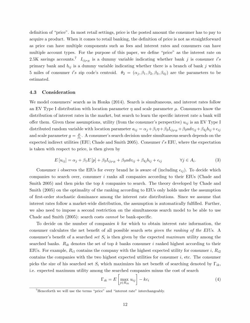
definition of “price”. In most retail settings, price is the posted amount the consumer has to pay to

acquire a product. When it comes to retail banking, the definition of price is not as straightforward

as price can have multiple components such as fees and interest rates and consumers can have

multiple account types. For the purpose of this paper, we define “price” as the interest rate on

2.5K savings accounts.7 IijPB is a dummy variable indicating whether bank j is consumer i′s

primary bank and bij is a dummy variable indicating whether there is a branch of bank j within

5 miles of consumer i′s zip code’s centroid. θ2 = (αj , β1, β2, β3, β4j) are the parameters to be

estimated.

4.3 Consideration

We model consumers’ search as in Honka (2014). Search is simultaneous, and interest rates follow

an EV Type I distribution with location parameter η and scale parameter µ. Consumers know the

distribution of interest rates in the market, but search to learn the specific interest rate a bank will

offer them. Given these assumptions, utility (from the consumer’s perspective) uij is an EV Type I

distributed random variable with location parameter aij = αj+β1η+β2IijPB +β3advij+β4jbij+εij

and scale parameter g = µβ1

. A consumer’s search decision under simultaneous search depends on the

expected indirect utilities (EIU; Chade and Smith 2005). Consumer i′s EIU, where the expectation

is taken with respect to price, is then given by

E [uij ] = αj + β1E [p] + β2IijPB + β3advij + β4jbij + εij ∀j ∈ Ai. (3)

Consumer i observes the EIUs for every brand he is aware of (including εij). To decide which

companies to search over, consumer i ranks all companies according to their EIUs (Chade and

Smith 2005) and then picks the top k companies to search. The theory developed by Chade and

Smith (2005) on the optimality of the ranking according to EIUs only holds under the assumption

of first-order stochastic dominance among the interest rate distributions. Since we assume that

interest rates follow a market-wide distribution, the assumption is automatically fulfilled. Further,

we also need to impose a second restriction on the simultaneous search model to be able to use

Chade and Smith (2005): search costs cannot be bank-specific.

To decide on the number of companies k for which to obtain interest rate information, the

consumer calculates the net benefit of all possible search sets given the ranking of the EIUs. A

consumer’s benefit of a searched set Si is then given by the expected maximum utility among the

searched banks. Rik denotes the set of top k banks consumer i ranked highest according to their

EIUs. For example, Ri1 contains the company with the highest expected utility for consumer i, Ri2

contains the companies with the two highest expected utilities for consumer i, etc. The consumer

picks the size of his searched set Si which maximizes his net benefit of searching denoted by Γik,

i.e. expected maximum utility among the searched companies minus the cost of search

Γik = E

[maxj∈Rik

uij

]− kci (4)

7Henceforth we will use the terms “price” and “interest rate” interchangeably.

12

where ci denotes consumer i′s search costs. We model search costs ci as a function of a con-

stant c0, demographics and the number of account types the consumer is planning to open.8 The

consumer picks the number of searches k which maximizes his net benefit of search.

4.4 Choice

After a consumer has formed his consideration set and learned the interest rates of the considered

banks, all uncertainty is resolved. At this stage, both the consumer and the researcher observe

interest rates. The consumer then picks the company with the highest utility among the searched

companies, i.e.

j = arg maxj∈Si

uij (5)

where uij now contains the actual interest rate for consumer i by bank j and Si is the set of

searched banks.

5 Identification

The identification strategy of the search model parameters follows closely Honka (2014). The

identification of the parameters capturing differences in brand intercepts, the effects of advertising,

price and bank branches that vary across companies is standard as in a conditional choice model.

These parameters also play a role in consumers’ consideration set decisions.

The size of a consumer’s consideration set helps pin down search costs. We can only identify a

range of search costs as it is utility-maximizing for all consumers with search costs in that range

to search a specific number of times. Beyond the fact that a consumer’s search cost lies within a

range which rationalizes searching a specific number of times, the variation in our data does not

identify a point estimate for search costs. The search cost point estimate will be identified by the

functional form of the utility function and the distributional assumption on the unobserved part of

the utility.

The base brand intercept is identified from the consumer’s decision to search or not to search.

Intuitively speaking, the option not to search and not to open (an) account(s) is the outside option

and allows us to identify the base brand intercept. So while the search cost estimate is pinned

down by the average number of searches, the base brand intercept is identified by the consumer’s

decision to search or not.

6 Estimation

The unconditional purchase probability is given by

Pij = PiAi · PiSi|Ai· Pij|Si

(6)

8The results when search costs vary with observed heterogeneity will be added to the next version of this paper.

13

In the following three subsections, we discuss how each of these probabilities are estimated.

Note that the awareness probability does not have any parameters or error terms in common with

the conditional consideration and conditional purchase probabilities. Thus it can be estimated

separately.

6.1 Awareness

Given our assumption on the error term ξij , we estimate Equation 1 as a multivariate logit regression

using the approach suggested by Russell and Petersen (2000). The probability that consumer i is

aware of bank j is given by

PiAi =exp (ς0j + ς1jadvij +Diς2 + bijς3j)

1 + exp (ς0j + ς1jadvij +Diς2 + bijς3j)(7)

where Ai is a vector of indicator variables capturing whether consumer i is aware of bank j.

Russell and Petersen (2000) have shown that a multivariate logic regression can be estimated by

maximizing the sum of the loglikelihoods of separate univariate binary logit regressions where each

univariate logit regression describes whether consumer i is aware of bank j for j = 1 . . . J . In order

for this approach to be equivalent to the estimation of a multivariate logit regression, we must

include consumer i′s awareness of all banks other than j as regressors in the univariate binary logit

regressions.

6.2 Consideration Given Awareness

We start by pointing out the crucial differences between what the consumer observes and what the

researcher observes:

1. While the consumer knows the distributions of prices in the market, the researcher does not.

2. While the consumer knows the sequence of searches, the researcher only partially observes

the sequence of searches by observing which banks are being searched and which ones are not

being searched.

3. In contrast to the consumer, the researcher does not observe εij .

Since the researcher does not observe the price distributions, these distributions need to be inferred

from the data. In other words, the typical assumption of rational expectations (e.g. Mehta, Rajiv,

and Srinivasan 2003, Hong and Shum 2006, Moraga-Gonzalez and Wildenbeest 2008, Honka 2014,

Honka and Chintagunta 2014) is that these distributions can be estimated from the prices observed

in the data. Given that the parameters of the price distributions are estimated, we need to account

for sampling error when estimating the other parameters of the model (see McFadden 1986).

To address the second issue, we point out that partially observing the sequence of searches

contains information that allows us to estimate the composition of consideration sets. Honka

(2014) has shown that the following condition has to hold for any searched set

14

minj∈Si

(E [uij ]) ≥ maxj′ /∈Si

(E[uij′])

∩ Γik ≥ Γik′ ∀k 6= k′ (8)

i.e. the minimum EIU among the searched brands is larger than the maximum EIU among the

non-searched brands and the net benefit of the chosen searched set of size k is larger than the net

benefit of any other search set of size k′.

We account for the fact that the researcher does not observe εij (point 3 above) by assuming that

εj has an EV Type I distribution with location parameter 0 and scale parameter 1 and integrating

over its distribution to obtain the corresponding probabilities with which we can compute the

likelihood function. Then the probability that a consumer picks a consideration set Si = Υ is

PiSi|ε = Pr

(minj∈Si

(E [uij ]) ≥ maxj′ /∈Si

(E[uij′])

∩ Γik ≥ Γik′ ∀k 6= k′)

(9)

6.3 Purchase Given Consideration

We now turn to the purchase decision stage given consideration. The consumer’s choice probability

conditional on his consideration set is

Pij|Si,ε =(uij ≥ uij′ ∀j 6= j′, j, j′ ∈ Si

)(10)

where we now include the actual prices in the utility function. Note that there is a selection

issue: given a consumer’s search decision, the εij do not follow an EV Type I distribution and the

conditional choice probabilities do not have a logit form. We solve this selection issue by using

SMLE when we estimate the conditional purchase probabilities.

In summary, the researcher estimates the price distributions, observes only partially the util-

ity rankings, and does neither observe ξij in the consumer’s awareness nor εij in the consumer’s

utility function. Given this, our estimable model has awareness probability given by Equation 7,

conditional consideration set probability given by Equation 9, and conditional purchase probability

given by Equation 10.

We maximize the joint likelihood of awareness set, consideration set, and purchase. The likeli-

hood of our model is given by

L =N∏i=1

[H∏h=1

P υihiAi

]·

∫ +∞

−∞

L∏l=1

J∏j=1

P ϑiliSi|Ai,ε· P δijij|Si,ε

f(ε) dε

(11)

where υih indicates the awareness set, ϑil indicates the chosen consideration set, and δij the

bank with which the consumer chooses to open an account with. θ = θ1, θ2, ci is the set of

parameters to be estimated. Neither the consideration set probability as shown is equation (9)

nor the purchase probability as shown in equation (10) have a closed-form solution. Honka (2014)

describes how to estimate this simultaneous search model in detail, and we follow her estimation

approach.

15

6.4 Advertising Endogeneity

One potential concern is advertising endogeneity. For example, banks may set advertising levels

according to their branches’ specific performance e.g. in terms of customer satisfaction. Since

customer satisfaction is not observed by the researcher, but may be observed by bank management,

this can give rise to advertising endogeneity concerns.

We collected data on the cost of advertisements at the DMA-level and will use these advertising

costs as exogenous shifters of advertising placement decisions. Since our model is highly nonlinear,

we are considering using the control function approach in the next version of the paper.

7 Results

7.1 Awareness

We start by discussing our results on consumer awareness for retail banks. Table 8 shows the

estimates from four multivariate logit regressions: Model (A1) includes bank fixed effects and

demographics and Model (A2) also includes advertising intensity. In Model (A3), we subsequently

control for bank branch presence. And, finally in Model (A4), we let the effects of advertising to

be bank-specific.9

In all four models, all bank fixed effects other than Bank of America in Model (A4) are signif-

icant. As expected, the big-4 banks (Bank of America, Citi, Chase, Wells Fargo) have relatively

higher brand awareness when compared to their more regional counterparts. In Model (A2), we find

a small positive coefficient of advertising (measured in 1, 000 units/placements) which decreases in

magnitude (but still remains significant) once we control for local bank branch dummies in Model

(A3). The effects of local branch presence are large and positive. In Model (A4), we see that even

after allowing for bank-specific coefficients on advertising the effects of local bank branch dummies

remain similar to the ones found in Model (A3). Further, we also see quite a bit of heterogeneity

in the effects of advertising across banks. The effects of advertising vary considerably in magni-

tude ranging from 0.0113 for Capital One to 1.4796 for Comerica Bank. Most interestingly, the

advertising coefficients for the big-4 banks (Bank of America, Citi, Chase, Wells Fargo) are all

insignificant. At this point in time, we speculate that the insignificant effects of advertising might

be due to diminishing returns of advertising as we observe banks which advertise more to have

smaller coefficient estimates. We will test this hypothesis in the next version of the paper by also

including squared advertising in the awareness function.

To quantify the effect of advertising, note that the average probability (across all banks and

consumers) of a consumer being aware of a bank is 32.46 percent. When advertising (measured in

1, 000 units/placements) is increased by 1 percent, the average probability (across all banks and

consumers) of a consumer being aware of a bank increases by 32.51 percent, i.e. an increase of 5 basis

9In Table 8, we show the estimation results for the awareness stage after shoppers and non-shoppers have been re-weighted to our data to be representative of the population. We also estimated our model with the non-representativesample and our results are similar.

16

points. These estimates also allow us to quantify the “brand awareness” value of the banks in terms

of advertising quantity. For example, in Model (A2), we find that Chase’s brand fixed effect is 2.2458

points above Citibank’s. Using the estimated advertising coefficient of 0.1624, this means the “brand

value gap” between Citi and BofA consists of 13, 829 advertisements (2.2458/0.1624 multiplied by

1,000). Moreover, note that the “branch presence” indicator coefficients are between 1 to 16

times the advertising coefficient (based on Model A4 estimates, focusing on significant coefficients),

suggesting that the presence of a branch is worth around 1,000 to 16,000 advertisements (assuming,

of course, that the advertising effect is linear throughout its domain).

=========================

Insert Table 8 about here

=========================

Finally, we also control for consumer demographics and find that the more thoroughly we control

for advertising and local bank presence, the fewer parameters associated with demographic variables

are significant. In Model (A4), only three demographics are significant: Asians and Hispanics are

aware of fewer banks than Whites and single/ divorced consumers have smaller awareness sets.

7.2 Consideration and Purchase

Models (LI-1) and (LI-2) in Table 9 show the estimates for the consideration and purchase parts

of the model. In Model (LI-2), we allow the effects of local bank branches to be bank-specific.10

Similarly to the results on awareness, we find all brand intercepts and bank branch dummies to

be significant. As expected, local bank presence increases consumers’ utility for a bank with the

effects ranging from 0.3839 for US Bank to 1.2999 for Keybank. Among the variables entering

consumers’ utility function, local bank presence is the second-largest utility shifter after interest

rates. Also, the estimated coefficients for local bank presence are much larger in magnitude than

the advertising coefficient and the coefficient on inertia (i.e. whether the consumer switches his

primary bank). Being a consumer’s primary bank, having high interest rates on savings accounts

and local bank presence increase consumer’s utility for a bank. While significant, the coefficient

for advertising is small and advertising is by far the smallest utility shifter. Thus we conclude that

advertising for retail banks only shifts consumer utility marginally.

=========================

Insert Table 9 about here

=========================

We find consumer search costs for retail banks (measured in interest-rate percentage points) to

be 0.09 percentage points (9 basis points) per bank searched, which translates to about $2.25 for a

10In Table 9, we show the estimation results for the consideration and purchase stages after shoppers and non-shoppers have been re-weighted to our data to be representative of the population. We also estimated our modelwith the non-representative sample and our results are similar.

17

2.5K account. Interestingly, this amount of search cost is comparable to other search cost estimates

in the financial products industry. For example, Hortacsu and Syverson (2004) found median search

costs to be between 7 and 21 basis points for S&P 500 index funds, which are typically purchased

by more financially sophisticated and higher-income individuals.

Based on the estimated coefficient for the “Primary Bank” dummy variable, switching costs

with regard to a consumer changing his primary bank appear to be an important factor of demand

in this market. The coefficient estimate on Primary Bank is about half of the coefficient estimates

for local bank presence which implies that branch closures have the potential to lead to consumers

switching their primary bank.

7.3 Does Advertising have an “Informative” or a “Persuasive” Role?

To compare the magnitudes of the effects of advertising across the different stages in the purchase

process, we calculate advertising elasticities for awareness and choice. Table 11 shows the results.

The average advertising elasticities for awareness and choice are 0.89 and 0.27, respectively. This

finding indicates that advertising rather affects consumer awareness than choice conditional on

awareness and that the role of advertising in the U.S. retail banking industry is primarily informa-

tive. Our results are similar to those found by previous literature albeit in different categories. For

example, Ackerberg (2001) and Ackerberg (2003) find that advertising has a primarily informative

role in the Yogurt market and Clark, Doraszelski, and Draganska (2009) also show that advertising

has stronger informative effects in a study of over 300 brands.

=========================

Insert Table 11 about here

=========================

Looking at the bank-specific advertising elasticities for awareness and choice, we find that the

advertising elasticities for awareness vary from 0.02 to 7.89, while the advertising elasticities for

choice conditional on awareness range from 0.00 to 1.15. For most banks, the advertising elasticity

for awareness is larger than that for choice. One important exception is Bank of America. Its

advertising elasticity for choice is about five times larger than that on awareness.11 Thus, for Bank

of America, the role of advertising is primarily persuasive.

7.4 Comparison with a Model under Full Information

In the previous sections, we developed and estimated a complete three-stage model of the consumer’s

shopping and account opening process that accounts for a consumer’s limited information. Doing

so only makes sense when limited information is an important factor in the decision-making process

and significantly influences results. To show the importance of accounting for limited information

11For Keybank and Capital One, the advertising elasticity for choice is also larger than that for awareness. Butthe difference in magnitudes is much smaller: In both cases, the advertising elasticity for choice is about twice aslarge as the advertising elasticity for awareness.

18

in the retail banking sector, we compare our estimates to those obtained from a model under full

information. In the full information model, we assume consumers are aware of and consider all

banks when deciding on the bank with which they would like to open (an) account(s) with (we

also allow for an outside option). Further, consumers know the actual interest rate any bank in the

data will offer them. Under these assumptions, the full information model can be estimated as a

multinomial logit model. The results are shown as Model (FI) in Table 9. Compared to the results

from the model under limited information, the coefficient estimates for local bank presence are two

to five times larger, the coefficient estimate for primary bank is negative and, most importantly,

the coefficient estimate on interest rates is also negative, i.e. consumers prefer savings accounts

with lower than higher interest rates, under the full information assumption.

The reason for the negative interest rate coefficient is the following: Recall that there are 18

banks in the retail banking sector and that consumers, on average, only consider 2.5 banks. When

demand is estimated under the full information assumption, in many cases consumers do not pick

the option with the highest or one of the highest interest rates among the 18 banks. Under full

information, this behavior is attributed to the consumer being insensitive to interest rates or, in this

specific case, even preferring lower to higher interest rates (holding everything else constant). Under

limited information, the model can distinguish between the consumer not picking a bank with a

high interest rate because he does not know about it (due to not being aware of or not considering

the bank) and the consumer being insensitive to interest rates. We conclude that it is essential to

account for consumers’ limited information in the retail banking sector to get meaningful demand

estimates.

7.5 Interest Rate Elasticities

Table 10 shows the own-interest rate elasticities implied by our limited information model. The

mean interest rate elasticity across all companies is 0.03 and the bank-specific interest rate elastici-

ties vary from 0.00 to 0.09. A strong contrast is found when the interest rate elasticities calculated

under limited information are compared to those estimated under full information. The average

own-interest rate elasticity under full information is -0.01. The negative sign of the interest rate

elasticity is counterintuitive and comes from the negative interest rate coefficient reported in Table

9 and discussed in the previous section.

=========================

Insert Table 10 about here

=========================

8 Counterfactuals

Note: We are currently working on the counterfactuals and results will be available in the next

version of the paper.

19

Note that our model is a partial equilibrium model. Thus any counterfactuals only capture

consequences on the demand side, i.e. we do not model interest rates or advertising spending

adjustments on the supply side. The results can be interpreted as short-run market effects.

8.1 Welfare Analysis

While informative advertising is viewed as “good,” there is some debate about whether persuasive

advertising actually provides consumers with any “real” utility. If persuasive advertising does not

yield any real utility, then we may ask what the socially optimal amount of informative advertising is

given that there are costs to advertising. In this counterfactual, we will study three scenarios: First,

we investigate what happens to market shares if either persuasive and/or informative advertising is

shut down and interest rates are fixed. Next, we allow interest rates to adjust in the same scenarios.

And finally, assuming that persuasive advertising does not yield any real utility to consumers, we

quantify the socially optimal amount of informative advertising. We then compare this with the

observed amount of informative advertising in the U.S. retail banking industry.

8.2 Free Interest Rates Comparison

Online price comparison sites such as pricegrabber.com or pricewatch.com where consumers can

costlessly see and compare product prices from different sellers are common for many products such

as groceries, appliances, electronics, toys, furniture and many more. Price comparison sites are less

common for financial services due to their complexity. Nevertheless, some innovative and largely

internet-based companies in other financial services areas such as Progressive and Esurance for

auto insurance are showing potential customers competitive price quotes on their own website thus

allowing them to costlessly see and compare prices. In this counterfactual, we investigate the effects

of the only internet bank, Capital One, newly introducing free local interest rate comparisons to

all potential customers visiting its website or bank branch, i.e. all customers who consider Capital

One.12

We investigate three different scenarios. First, we study the effects of the interest rate com-

parison tool introduction by itself, i.e. without any changes to the other variables. Next, suppose

Capital One accompanied the interest rate comparison tool introduction by doubling the number

of advertisements they are showing. And finally, we investigate what the necessary increase in

advertisements would be to triple Capital One’s market share to 10 percent.

9 Robustness Checks

We conduct a variety of checks to test the robustness of our results. First, we change the radius

for the local bank branch variable in the estimation. Currently, we control for local bank presence

by including an indicator variable that reflects whether there is at least one bank branch within

12Capital One only had 854 bank branches in the U.S. (in 2010), with over 70 percent of them being located inthe states of New York, Texas and Louisiana.

20

5 miles of the consumer’s zip code’s centroid. We also estimated our model using an alternative

radius of 10 miles from the consumer’s zip code’s centroid for local bank presence. The results are

shown in Tables 12 for awareness and Table 13 for consideration and choice. For both awareness

and consideration and choice, we find very similar and for most significant bank branch dummies

slightly larger coefficients using the 10-miles radius compared to the 5-miles radius. The estimates

for the other variables remain very similar. Thus we conclude that our results are robust to different

definitions of local bank presence.

=========================

Insert Table 12 about here

=========================

=========================

Insert Table 13 about here

=========================

Second, we also verified the robustness of our results to an alternative definition of interest

rates. The current reported results are based on interest rate data calculated using information

on the top 2.5K savings account for each bank. But we also experimented using data on all 2.5K

savings accounts that each bank has, and the results did not change significantly.

And lastly, we check the robustness of our results with respect to a different measure of ad-

vertising. In our model, we operationalize advertising as the sum of national and DMA-level

advertisements. In this robustness check, we only use the DMA-level advertising quantity in the

estimation. We find that our results are qualitatively and largely also quantitatively robust to this

alternative measure of advertising.

10 Limitations and Future Research

There are several limitations to our research. First, our model describes the consumer’s shopping

and account opening process given the consumer’s decision on account types he is considering

adding or moving, i.e. we do not model jointly the consumer’s choice of account types and the

search among banks. Our model assumes that consumers first decide which account types to

add/move and then begin the shopping process. It is left for future research to develop a model

where consumers choose several products and search at the same time that they evaluate those

products. Second, we use the interest rates for 2.5K savings account as a proxy for price. While

this is a reasonable assumption, a more precise price measure potentially self-reported by consumers

would further advance our understanding of consumers’ shopping process for bank accounts.

Third, we assume consumers have rational expectations about the distribution of interest rates

for all banks that they are aware of. A model that has information on consumer expectations for

interest rates or is able to recover them would enable researchers to test the hypothesis of rational

21

expectations. And lastly, more work is needed to enhance our understanding of the effectiveness

of price promotions versus advertising in the retail banking industry. Advertisements stating, for

example, that consumers can get $200 for opening a new checking account as advertised by Chase,

are effectively price promotions and their effectiveness as compared to brand advertising is an open

question. We leave it to future research to find the answer to this question.

11 Conclusion

In this paper, we utilize a unique data set with detailed info on consumers’ shopping process for

banking services. Using data on awareness and consideration sets and the purchase decision, we

attempt to disentangle the informative and persuasive effects of advertising in the retail banking

sector. We find advertising primarily informs consumers about the existence of banks and their

products and does not shift consumers’ utility for retail banking products. We also find that branch

presence is a very effective driver of awareness and choice (upon consideration), reflecting the local

nature of banking (consistent with the fact that banks that operate mostly through the internet

have had very little penetration in the U.S.). Consumers face nontrivial search costs in this market,

equivalent to 0.09 percentage points in interest rate terms. Switching costs away from the primary

bank also appear to be an important factor of demand in this market, though with a similar order

of magnitude to local bank presence – i.e. (multiple) branch closures would easily lead to switching

to a different bank. We hope that our (still preliminary) results shed light on the drivers of demand

in this very important sector of the economy, and we hope to seek further managerial and policy

implications of our demand estimates in the near future.

22

References

Abhishek, Vibhanshu, Peter Fader, and Kartik Hosanagar (2012), “The Long Road to Online

Conversion: A Model of Multi-Channel Attribution,” Working paper, Carnegie Mellon University.

Ackerberg, Daniel A (2001), “Empirically distinguishing informative and prestige effects of adver-

tising,” RAND Journal of Economics, 316–333.

Ackerberg, Daniel A. (2003), “Advertising, learning, and consumer choice in experience good mar-

kets: an empirical examination*,” International Economic Review, 44 (3), 1007–1040.

Allen, Jason, Robert Clark, and Jean-Francois Houde (2012), “Price Negotiation in Differentiated

Products Markets: Evidence from the Canadian Mortgage Market,” Working Papers 12-30, Bank

of Canada.

Allenby, Greg M. and James L. Ginter (1995), “The effects of in-store displays and feature ad-

vertising on consideration sets,” International Journal of Research in Marketing, 12 (1), 67 –

80.

Bagwell, Kyle (2007), The Economic Analysis of Advertising, volume 3 of Handbook of Industrial

Organization, Elsevier.

Chade, Hector and Lones Smith (2005), “Simultaneous Search,” Working paper.

Chamberlin, Edward (1933), The Theory of Monopolistic Competition: A Re-orientation of the

Theory of Value, Harvard University Press.

Chan, Tat, Chakravarthi Narasimhan, and Ying Xie (2013), “Treatment Effectiveness and Side

Effects: A Model of Physician Learning,” Management Science, 59 (6), 1309–1325.

Chiang, Jeongwen, Siddhartha Chib, and Chakravarthi Narasimhan (1998), “Markov chain Monte

Carlo and models of consideration set and parameter heterogeneity,” Journal of Econometrics,

89, 223 – 248.

Ching, Andrew T. and Masakazu Ishihara (2012), “Measuring the Informative and Persuasive Roles

of Detailing on Prescribing Decisions,” Management Science, 58 (7), 1374–1387.

Clark, C.Robert, Ulrich Doraszelski, and Michaela Draganska (2009), “The effect of advertis-

ing on brand awareness and perceived quality: An empirical investigation using panel data,”

Quantitative Marketing and Economics, 7 (2), 207–236.

Cohen, Michael and Marc Rysman (2013), “Payment choice with consumer panel data,” Working

Papers 13-6, Federal Reserve Bank of Boston.

De los Santos, Babur I., Ali Hortacsu, and Matthijs R. Wildenbeest (2012), “Testing Models of

Consumer Search Using Data on Web Browsing and Purchasing Behavior,” American Economic

Review, 102 (6), 2955–80.

23

Dick, Astrid A. (2007), “Market Size, Service Quality, and Competition in Banking,” Journal of

Money, Credit and Banking, 39 (1), 49–81.

— (2008), “Demand estimation and consumer welfare in the banking industry,” Journal of Banking

& Finance, 32 (8), 1661–1676.

Franses, Philip H. and Marco Vriens (2004), “Advertising effects on awareness, consideration and

brand choice using tracking data,” Working paper, Erasmus Research Institute of Management

(ERIM).

Goeree, Michelle Sovinsky (2008), “Limited information and advertising in the US personal com-

puter industry,” Econometrica, 76 (5), 1017–1074.

Gurun, Umit G., Gregor Matvos, and Amit Seru (2013), “Advertising Expensive Mortgages,”

Working paper, National Bureau of Economic Research.

Hastings, Justine S., Ali Hortacsu, and Chad Syverson (2013), “Advertising and Competition in

Privatized Social Security: The Case of Mexico,” Working paper, National Bureau of Economic

Research.

Hirtle, Beverly (2007), “The impact of network size on bank branch performance,” Journal of

Banking & Finance, 31 (12), 3782–3805.

Hong, Han and Matthew Shum (2006), “Using price distributions to estimate search costs,” The

RAND Journal of Economics, 37 (2), 257–275.

Honka, Elisabeth (2014), “Quantifying Search and Switching Costs in the U.S. Auto Insurance

Industry,” The RAND Journal of Economics, Forthcoming.

Honka, Elisabeth and Pradeep K. Chintagunta (2014), “Simultaneous or Sequential? Search Strate-

gies in the U.S. Auto Insurance Industry,” Working paper.

Hortacsu, Ali and Chad Syverson (2004), “Product Differentiation, Search Costs, and Competition

in the Mutual Fund Industry: A Case Study of S&P 500 Index Funds,” The Quarterly Journal

of Economics, 119 (2), 403–456.

Kim, Jun B., Paulo Albuquerque, and Bart J. Bronnenberg (2010), “Online Demand Under Limited

Consumer Search,” Marketing Science, 29 (6), 1001–1023.

Koulayev, Sergei, Marc Rysman, Scott Schuh, and Joanna Stavins (2012), “Explaining adoption

and use of payment instruments by U.S. consumers,” Working paper, Federal Reserve Bank of

Boston.

Lee, Jonathan, J. Han, C. Park, and Pradeep K. Chintagunta (2005), “Modeling pre-diffusion

process with attitudinal trackings and expert ratings: trackings and expert ratings: Forecasting

opening weekend box-office,” Working paper.

24

Lovett, Mitchell J. and Richard Staelin (2012), “The Role of Paid and Earned Media in Building

Entertainment Brands: Reminding, Informing, and Enhancing Enjoyment,” Working paper,

Simon School of Business – University of Rochester.

McFadden, Daniel (1986), “The Choice Theory Approach to Market Research,” Marketing Science,

5 (4), 275–297.

Mehta, Nitin, Surendra Rajiv, and Kannan Srinivasan (2003), “Price Uncertainty and Consumer

Search: A Structural Model of Consideration Set Formation,” Marketing Science, 22 (1), 58–84.

Molnar, Jozsef, Roberto Violi, and Xiaolan Zhou (2013), “Multimarket contact in Italian retail

banking: Competition and welfare,” International Journal of Industrial Organization, 31 (5),

368 – 381.

Moraga-Gonzalez, Jose L. and Matthijs R. Wildenbeest (2008), “Maximum likelihood estimation

of search costs,” European Economic Review, 52 (5), 820–848.

Muir, David M., Katja Seim, and Maria Ana Vitorino (2013), “Price Obfuscation and Consumer

Search: An Empirical Analysis,” Working paper.

Narayanan, Sridhar, Puneet Manchanda, and Pradeep K. Chintagunta (2005), “Temporal Differ-

ences in the Role of Marketing Communication in New Product Categories,” Journal of Marketing

Research, 42 (3), 278–290.

Russell, Gary J and Ann Petersen (2000), “Analysis of cross category dependence in market basket

selection,” Journal of Retailing, 76 (3), 367 – 392.

Rysman, Marc (2007), “An Empirical Analysis of Payment Card Usage,” The Journal of Industrial

Economics, 55 (1), 1–36.

Rysman, Marc and Julian Wright (2012), “The Economics of Payment Cards,” Working paper,

Boston University.

Siddarth, S., Randolph E. Bucklin, and Donald G. Morrison (1995), “Making the Cut: Modeling

and Analyzing Choice Set Restriction in Scanner Panel Data,” Journal of Marketing Research,

32 (3), pp. 255–266.

Terui, Nobuhiko, Masataka Ban, and Greg M. Allenby (2011), “The Effect of Media Advertising

on Brand Consideration and Choice,” Marketing Science, 30 (1), 74–91.

van Nierop, Erjen, Bart J. Bronnenberg, Richard Paap, Michel Wedel, and Philip Hans Franses

(2010), “Retrieving Unobserved Consideration Sets from Household Panel Data,” Journal of

Marketing Research, 47 (1), pp. 63–74.

Wang, Hui (2010), “Consumer Valuation of Retail Networks: Evidence from the Banking Industry,”

Working paper, Peking University.

25

Winer, Russel S. and Ravi Dhar (2011), Marketing Management, Upper Saddle River, NJ: Prentice

Hall, 4th edition edition.

Zhang, Jie (2006), “An Integrated Choice Model Incorporating Alternative Mechanisms for Con-

sumers’ Reactions to In-Store Display and Feature Advertising,” Marketing Science, 25 (3), pp.

278–290.

26

Tables and Figures

Figure 1: Number of Accounts Opened

Figure 2: Size of awareness sets

27

Figure 3: Size of shoppers’ consideration sets

Figure 4: Awareness vs Consideration (Shoppers only)

28

Figure 5: Size of awareness sets

Figure 6: Awareness vs Consideration (Shoppers only)

29

Figure 7: Geographic Distribution of Banks’ DMA-level Advertising (Expenditures)

This map displays the spatial distribution of DMA-level advertising expenditure by banks in the 206 DMAs across

the U.S. over the reference period. Areas in white correspond to DMAs for which Kantar Media does not collect

data. Advertising numbers in the legend are represented in thousands.

Figure 8: Geographic Distribution of Banks’ DMA-level Advertising (Placements)

This map displays the spatial distribution of DMA-level number of advertising placements by banks in the 206 DMAs

across the U.S. over the reference period. Areas in white correspond to DMAs for which Kantar Media does not

collect data.

30

Table 1: Share of respondents that were Aware/Considered/Chose each Bank (%)

This table presents the percentage of respondents in the sample that were Aware, Considered or Chose each of the

institutions listed.

Institution Aware Considered Chose

BB&T 17.15 5.44 3.13Bank Of America 95.18 44.27 12.52Capital One 31.89 6.55 3.32Chase/WaMu 73.94 32.18 12.62Citibank 63.87 17.92 7.27Citizens Bank 25.24 7.71 4.53Comerica Bank 10.98 1.93 0.87Fifth Third Bank 25.39 7.80 3.71HSBC 21.53 7.56 3.03Keybank 24.18 6.12 2.99M&T 8.62 4.19 2.31PNC/National City Bank 34.92 11.03 4.67Regions Bank 21.10 5.97 3.08Sovereign Bank 17.68 4.82 2.26Suntrust Bank 31.12 11.66 7.61TD Bank 21.48 8.96 4.05U.S. Bank 31.21 13.01 8.33Wells Fargo/Wachovia 87.24 34.39 13.68

31

Table 2: Demographics for full and selected samples

This table compares the demographics of the respondents in the selected sample with all of the survey respondents.

Columns “All Respondents” and “Selected Sample” report the percentage of respondents in each of the demographic

groups for all of the survey respondents and for the selected sample respectively.

Data setAll Respondents Selected Sample

(n = 4, 246) (n = 2, 076)% %

GenderFemale 60.0 60.8Male 40.0 39.2

Age19-29 17.0 17.930-44 30.4 32.345-59 34.0 32.460+ 18.7 17.4

Household IncomeUnder $49,999 36.5 35.5$50,000-$99,999 38.0 38.2$100,000 and over 25.5 26.3

RaceWhite 81.3 78.1Black 5.0 5.6Asian 7.5 9.3Hispanic 3.9 5.0Other 2.3 2.0

EducationHigh school or less 8.5 7.2Some College 32.2 31.0College graduate 29.4 31.4Postgraduate 29.9 30.4

Marital StatusSingle/Divorced 33.4 33.3Married/Partner 63.7 64.5Widowed 2.9 2.2

RegionNew England 5.6 6.5MidAtlantic 22.9 28.3Midwest 10.5 6.7North Central 10.9 8.8Southeast 8.1 8.0South Central 4.1 3.1Texas 4.1 4.6Florida 8.8 10.8Southwest 6.3 5.9Northwest 4.3 4.5California 12.8 12.7Other 1.6 0.132

Table 3: Demographics by Respondent Type

This table reports descriptive statistics for all respondents in our final sample as well as for the two subgroups

of respondents: “shoppers” (1,832 consumers) and “non-shoppers” (244 consumers). Shoppers are consumers who

opened one or more new accounts and non-shoppers are consumers who did not open new accounts during the

reference period.

Respondent TypeShopper Non Shopper All

% % %

GenderFemale 60.9 59.8 60.8Male 39.1 40.2 39.2

Age19-29 19.6 5.3 17.930-44 34.2 17.6 32.345-59 30.8 43.9 32.460+ 15.3 33.2 17.4

Household IncomeUnder $49,999 34.0 47.1 35.5$50,000-$99,999 38.9 32.8 38.2$100,000 and over 27.1 20.1 26.3

RaceWhite 76.9 86.9 78.1Black 5.8 3.7 5.6Asian 10.0 3.7 9.3Hispanic 5.4 2.0 5.0Other 1.8 3.7 2.0

EducationHigh school or less 6.4 12.7 7.2Some College 30.5 35.2 31.0College graduate 32.0 26.2 31.4Postgraduate 31.1 25.8 30.4

Marital StatusSingle/Divorced 33.7 30.7 33.3Married/Partner 64.3 65.6 64.5Widowed 2.0 3.7 2.2

RegionRegionNew England 6.8 4.1 6.5MidAtlantic 29.3 20.5 28.3Midwest 5.6 15.6 6.7North Central 8.2 12.7 8.8Southeast 8.2 6.6 8.0South Central 2.8 5.7 3.1Texas 4.5 5.3 4.6Florida 11.2 7.8 10.8Southwest 5.8 6.6 5.9Northwest 4.5 4.5 4.5California 12.9 10.7 12.7Other 0.2 0.0 0.1

33

Table 4: Account types opened (Shoppers only)

This table shows, for the subsample of shoppers, the types of new accounts opened during the reference period.

% Respondents % RespondentsAccount type Opening Account type Opening

Deposit Accounts Borrowing AccountsChecking 85.10 Credit Card 25.87Savings 57.86 Mortgage 9.01Certificate of Deposit 11.74 Home Equity Loan 6.28Money Market Account 12.45 Personal Loan 8.02

Investment AccountsMutual Funds 4.69Stocks/Bonds 4.26

Table 5: Respondents with bank branches within 5 miles of their home (Shoppersonly)

This table reports the percentage of shoppers in the sample with bank branches within 5 miles of their home conditional

on them having Considered/Chosen each of the institutions listed.

Institution Considered Chosen

BB&T 84.82 82.81Bank Of America 85.52 86.26Capital One 69.63 67.65Chase/WaMu 88.08 90.58Citibank 69.92 78.38Citizens Bank 60.00 60.71Comerica Bank 86.84 87.50Fifth Third Bank 80.39 85.29HSBC 42.38 47.37Keybank 85.25 91.23M&T 84.81 85.00PNC/National City Bank 86.18 88.24Regions Bank 88.33 91.67Sovereign Bank 78.95 80.95Suntrust Bank 86.02 87.50TD Bank 90.76 92.68U.S. Bank 82.00 88.24Wells Fargo/Wachovia 88.65 91.44

34

Table 6: Interest Rates by Institution

This table reports summary statistics for the interest rates associated with the most popular 2.5K savings accounts

for each bank. These rates proxy for the actual rates that each respondent obtained upon searching over the banks in

his consideration set. Interest rates statistics are calculated using banks in respondents consideration sets and based

on respondents’ zip codes. N is the number of respondents that considered a given bank.

Institution mean sd min max N

BB&T 0.050 0.000 0.050 0.050 113Bank Of America 0.100 0.000 0.100 0.100 919Capital One 1.101 0.439 0.050 1.290 136Chase/WaMu 0.010 0.000 0.010 0.010 668Citibank 0.290 0.169 0.250 1.000 372Citizens Bank 0.050 0.000 0.050 0.050 160Comerica Bank 0.050 0.000 0.050 0.050 40Fifth Third Bank 0.200 0.000 0.200 0.200 162HSBC 0.050 0.000 0.050 0.050 157Keybank 0.050 0.000 0.050 0.050 127M&T 0.050 0.000 0.050 0.050 87PNC/National City Bank 0.050 0.000 0.050 0.050 136Regions Bank 0.100 0.000 0.100 0.100 124Sovereign Bank 0.100 0.000 0.100 0.100 100Suntrust Bank 0.050 0.000 0.050 0.050 242TD Bank 0.100 0.000 0.100 0.100 186U.S. Bank 0.100 0.000 0.100 0.100 270Wells Fargo/Wachovia 0.046 0.007 0.030 0.050 345

35

Table 7: DMA-Level Advertising Expenditures (dols000) and Placements by Bank

This table shows average advertising expenditures and average number of placements (also called “units”) by bank.

It includes Spot TV, Newspapers, National Spot Radio, Internet Display, Outdoor at DMA-level. The averages are

taken by dividing the total advertising expenditures/placements at the DMA-level over the entire reference period

by the number of DMAs in which each bank had some advertising activity.

Institution Average per DMA Number of DMAsExpenditure Units

BB&T 207.0 188.9 23Bank Of America 424.0 1859.0 101Capital One 432.2 895.9 97Chase/WaMu 1039.7 1376.0 98Citibank 654.4 333.2 99Citizens Bank 258.2 234.5 99Comerica Bank 336.2 271.2 16Fifth Third Bank 797.7 1526.3 30HSBC 209.5 286.0 97Keybank 415.6 1464.2 29M&T 390.2 615.4 14PNC/National City Bank 525.6 770.6 99Regions Bank 254.2 353.4 43Sovereign Bank 117.0 154.4 65Suntrust Bank 336.3 501.7 83TD Bank 848.5 810.2 43U.S. Bank 154.1 183.2 79Wells Fargo/Wachovia 433.2 1084.7 101

36

Table 8: Results from Awareness Stage

This table reports the results from four different model specifications for the Awareness stage. Panel A reports the

Brand, Branches and Advertising Parameters and Panel B reports the parameters associated with the demographic

variables. All four models include bank-specific fixed effects.“Branch presence” is operationalized as a dummy variable

that captures whether there is a branch of a given bank present within 5-miles of each respondent zip-code centroid.

Advertising corresponds to the number of DMA placements. Advertising is not included in model (A1) and in Model

(A4) is allowed to have coefficients that are bank-specific. The omitted demographic categories are Married/Partner,

White, Income below 50k and High school or less for the variables Marital Status, Race, Income and Education,

respectively. Standard-errors are reported in parentheses under coefficient estimates. (**) and (*) denote statistical

significance for 5% and 10% levels respectively.

Panel A: Brand, Branches and Advertising Parameters

(A1) (A2) (A3) (A4)Brand Brand Brand Branch Brand Branch Advert

presence presence

Bank of America -1.530** -23.109** -9.997** 0.385 -11.726 0.076 0.355(0.257) (1.201) (1.005) (0.301) (7.216) (0.055) (0.315)

BB&T -5.141** -5.363** -5.475** 1.149** -5.424** 0.300 1.147**(0.488) (0.498) (0.512) (0.201) (0.512) (0.540) (0.227)

Citibank -2.399** -7.171** -4.709** 1.620** -4.755** 0.064 1.615**(0.249) (0.364) (0.340) (0.165) (1.244) (0.040) (0.175)

Citizens Bank -3.806** -6.846** -5.687** 1.732** -15.985** 0.666** 1.434**(0.350) (0.398) (0.403) (0.215) (2.295) (0.132) (0.225)

Comerica -5.010** -4.882** -5.817** 2.472** -6.821** 1.480** 1.522**(0.556) (0.545) (0.581) (0.206) (0.632) (0.198) (0.238)

Fifth Third -3.640** -4.130** -5.031** 2.919** -5.321** 0.453** 2.198**(0.339) (0.349) (0.399) (0.213) (0.413) (0.078) (0.240)

HSBC -4.028** -9.118** -6.022** 1.400** -17.702** 0.392** 0.953**(0.380) (0.472) (0.453) (0.228) (3.160) (0.089) (0.268)

Chase -3.525** -4.925** -4.209** 0.602** -4.078** 0.046 0.654**(0.257) (0.273) (0.282) (0.136) (0.377) (0.034) (0.167)

Keybank -3.083** -3.457** -4.225** 2.742** -4.389** 0.222** 2.429**(0.311) (0.319) (0.347) (0.179) (0.354) (0.050) (0.202)

M&T -7.354** -8.218** -8.540** 0.841** -9.246** 0.822** 0.677**(0.711) (0.753) (0.785) (0.260) (0.827) (0.171) (0.267)

PNC/N. City Bank -3.955** -19.999** -10.709** 1.582** -8.330** 0.039 1.630**(0.295) (0.930) (0.774) (0.147) (2.677) (0.027) (0.153)

Regions -4.266** -5.041** -5.516** 2.360** -6.475** 0.300** 1.554**(0.398) (0.406) (0.438) (0.199) (0.482) (0.035) (0.225)

Sovereign -4.693** -4.891** -5.468** 1.912** -5.529** 0.108* 1.832**(0.422) (0.415) (0.450) (0.216) (0.484) (0.065) (0.230)

SunTrust -3.401** -3.907** -5.131** 4.048** -6.484** 0.898** 2.613**(0.329) (0.338) (0.393) (0.267) (0.476) (0.134) (0.334)

TD -4.662** -5.809** -6.556** 2.406** -6.964** 0.131** 2.077**(0.406) (0.408) (0.467) (0.236) (0.554) (0.038) (0.283)

US Bank -2.491** -3.013** -4.596** 2.871** -5.525** 0.366** 2.819**(0.306) (0.311) (0.363) (0.183) (0.512) (0.123) (0.192)

Wells Fargo/Wachovia -3.314** -7.087** -5.288** 0.933** -5.707** 0.081** 0.918**(0.260) (0.335) (0.339) (0.190) (0.732) (0.032) (0.202)

Capital One -3.694** -10.427** -6.839** 1.586** -4.781** 0.011 2.446**(0.310) (0.491) (0.456) (0.264) (0.465) (0.008) (0.279)

Advertising 0.162** 0.063**(0.009) (0.007)

37

Table 8: Results from Awareness Stage (cont.)

Panel B: Demographics’ Parameters

(A1) (A2) (A3) (A4)

Gender – Male 0.002 -0.004 -0.044 -0.045(0.038) (0.038) (0.041) (0.041)

Age -0.001 0.000 0.001 0.001(0.001) (0.001) (0.002) (0.002)

Marital Status

Single/ Divorced 0.004 -0.033 -0.090* -0.094**(0.043) (0.043) (0.046) (0.047)

Widow -0.110 -0.167 -0.163 -0.154(0.123) (0.126) (0.133) (0.135)

Race

Black -0.059 -0.063 -0.086 -0.103(0.080) (0.081) (0.087) (0.088)

Asian -0.101 -0.166** -0.235** -0.235**(0.067) (0.069) (0.073) (0.074)

Hispanic -0.140 -0.213** -0.275** -0.279**(0.088) (0.091) (0.097) (0.097)

Other -0.062 -0.096 -0.197 -0.188(0.130) (0.133) (0.141) (0.142)

Income

Income 50k - 100k 0.110** 0.050 0.040 0.029(0.044) (0.045) (0.048) (0.048)

Income above 100k 0.163** 0.093* 0.030 0.027(0.052) (0.053) (0.056) (0.057)

Education

Some College 0.072 0.082 0.033 0.059(0.075) (0.076) (0.080) (0.081)

College Degree 0.138* 0.141* 0.005 0.027(0.076) (0.077) (0.082) (0.083)

Adv. Degree 0.133* 0.130* -0.022 -0.002(0.077) (0.078) (0.083) (0.083)

* p < 0.10; ** p < 0.05

38

Table 9: Results from Consideration and Purchase Stages

This table reports the results from three different model specifications for the Consideration and Purchase stages.

Specification (FI) corresponds to a Full Information Model, equivalent to a traditional multinomial logit model, in

which consumers are assumed to be aware and consider all banks and know what are banks’ actual interest rates

without engaging in search. Specifications (LI) correspond to models that account for consumers’ Limited Information.

In model (LI-1) branch presence is operationalized as a dummy variable that captures whether there is a branch of

a given bank present within 5-miles of each respondent zip-code centroid and in model (LI-2) branch coefficients are

allowed to be bank-specific. Standard-errors are reported in parentheses under coefficient estimates. (**) and (*)

denote statistical significance for 5% and 10% levels respectively.

(FI) (LI-1) (LI-2)Brand Branches Brand Brand Branches

Bank of America -2.266** 1.661** -3.259** -3.668** 0.682**(0.583) (0.212) (0.121) (0.056) (0.169)

BB&T -2.694** 3.339** -1.914** -1.926** 0.920**(0.311) (0.339) (0.064) (0.244) (0.278)

Citibank -1.793** 2.612** -2.316** -2.608** 1.133**(0.230) (0.209) (0.072) (0.160) (0.175)

Citizens Bank -1.731** 2.271** -1.801** -1.826** 0.797**(0.197) (0.236) (0.070) (0.197) (0.246)

Comerica -4.436** 4.091** -2.712** -3.191* 1.435(0.706) (0.755) (0.153) (1.707) (1.710)

Fifth Third -2.760** 3.494** -2.209** -2.034** 0.685**(0.329) (0.349) (0.083) (0.265) (0.284)

HSBC -2.038** 2.115** -1.848** -1.781** 0.462*(0.233) (0.274) (0.066) (0.215) (0.258)

Chase -1.657** 2.503** -1.951** -2.261** 1.237**(0.234) (0.237) (0.061) (0.189) (0.191)

Keybank -3.468** 4.001** -2.215** -2.563** 1.300**(0.453) (0.473) (0.080) (0.271) (0.301)

M&T -3.321** 3.685** -1.567** -1.475** 0.826(0.415) (0.449) (0.167) (0.684) (0.725)

PNC/N. City Bank -3.373** 2.828** -3.028** -3.526** 0.976**(0.475) (0.342) (0.060) (0.198) (0.230)

Regions -3.509** 4.248** -2.183** -2.409** 1.110**(0.454) (0.474) (0.089) (0.339) (0.359)

Sovereign -3.037** 3.329** -2.101** -1.819** 0.469(0.362) (0.400) (0.084) (0.370) (0.392)

SunTrust -2.177** 3.884** -1.688** -1.861** 1.126**(0.241) (0.256) (0.096) (0.397) (0.404)

TD -3.258** 3.859** -1.819** -1.687** 0.685*(0.416) (0.429) (0.111) (0.349) (0.358)

US Bank -2.073** 3.039** -1.910** -1.445** 0.384(0.250) (0.259) (0.086) (0.265) (0.277)

Wells Fargo/Wachovia -1.803** 2.439** -2.263** -2.680** 1.298**(0.261) (0.248) (0.069) (0.184) (0.188)

Capital One -2.222** 2.706** -2.622** -2.672** 0.538**(0.407) (0.298) (0.119) (0.201) (0.228)

Other parameters

Primary Bank -0.763** 0.422** 0.415**(0.090) (0.038) (0.060)

Interest Rates -0.107 0.950** 0.982**(0.276) (0.163) (0.230)

Advertising 0.009** 0.009** 0.014**(0.004) (0.001) (0.006)

Bank Branches 0.924**(0.045)

Search Cost Constant 0.001** 0.001**(0.000) (0.000)

39

Table 10: Interest Rate Elasticities

This table reports the price (i.e. interest rate) elasticities that correspond to the model estimates reported in Table

9. Specification (FI) corresponds to a Full Information Model, equivalent to a traditional multinomial logit model,

in which consumers are assumed to be aware and consider all banks and know what are banks’ actual interest

rates without engaging in search. Specification (LI-2) corresponds to a model that account for consumers’ Limited

Information in which branch presence is operationalized as a dummy variable that captures whether there is a branch

of a given bank present within 5-miles of each respondent zip-code centroid. Elasticities are calculated for each

respondent and bank and then averaged across respondents.

(FI) (LI-2)Brand

Bank of America -0.01 0.06BB&T 0.00 0.03Citibank -0.03 0.18Citizens Bank 0.00 0.03Comerica -0.01 0.04Fifth Third -0.02 0.12HSBC -0.01 0.03Chase 0.00 0.01Keybank 0.00 0.03M&T 0.00 0.03PNC/N. City Bank 0.00 0.02Regions -0.01 0.06Sovereign -0.01 0.07SunTrust 0.00 0.03TD -0.01 0.06US Bank -0.01 0.06Wells Fargo/Wachovia 0.00 0.02Capital One -0.10 0.48

Average -0.01 0.07

40

Table 11: Advertising Elasticities

This table reports the advertising elasticities that correspond to the model estimates reported in Tables 8 and 9.

Elasticities are calculated for each respondent and bank and then averaged across respondents.

Awareness Choice

(4) (LI-2)Brand

Bank of America 0.22 1.15BB&T 0.02 0.00Citibank 0.73 0.28Citizens Bank 2.69 0.15Comerica 0.14 0.02Fifth Third 0.04 0.03HSBC 7.89 0.34Chase 0.14 0.08Keybank 0.02 0.04M&T 0.06 0.01PNC/N. City Bank 0.85 0.84Regions 0.27 0.08Sovereign 0.10 0.04SunTrust 0.52 0.03TD 0.22 0.09US Bank 1.45 0.03Wells Fargo/Wachovia 0.23 0.20Capital One 0.17 0.36

Average 0.89 0.27

41

Table 12: Results from Awareness Stage - Robustness

This table reports the results of robustness checks for two of the Awareness stage model results shown in table 8.

Here “Branch presence” is operationalized as a dummy variable that captures whether there is a branch of a given

bank present within 10-miles (as opposed to 5-miles) of each respondent zip-code centroid. Panel A reports the

Brand, Branches and Advertising Parameters and Panel B reports the parameters associated with the demographic

variables. Standard-errors are reported in parentheses under coefficient estimates. (**) and (*) denote statistical

significance for 5% and 10% levels respectively.

Panel A: Brand, Branches and Advertising Parameters

(A3-R) (A4-R)Brand Branch Brand Branch Advert

presence presence

Bank of America -8.024** 0.150 -13.291* 0.068 0.090(0.998) (0.328) (7.169) (0.341) (0.054)

BB&T -5.560** 1.297** -5.567** 1.304** 0.265(0.518) (0.224) (0.518) (0.249) (0.534)

Citibank -4.464** 1.753** -4.620** 1.731** 0.055(0.341) (0.161) (1.203) (0.169) (0.039)

Citizens Bank -5.588** 1.709** -15.958** 1.398** 0.658**(0.407) (0.205) (2.293) (0.215) (0.132)

Comerica -6.202** 2.575** -6.929** 1.365** 1.492**(0.594) (0.224) (0.629) (0.273) (0.214)

Fifth Third -4.966** 2.812** -5.310** 2.079** 0.476**(0.394) (0.200) (0.410) (0.227) (0.078)

HSBC -5.685** 1.381** -17.160** 0.991** 0.373**(0.453) (0.212) (3.174) (0.248) (0.089)

Chase -4.143** 0.629** -4.203** 0.609** 0.058*(0.285) (0.138) (0.374) (0.164) (0.033)

Keybank -4.414** 2.541** -4.557** 2.205** 0.218**(0.350) (0.163) (0.357) (0.189) (0.050)

M&T -8.659** 0.995** -9.533** 0.870** 0.873**(0.803) (0.317) (0.851) (0.324) (0.172)

PNC/N. City Bank -9.666** 1.881** -5.298** 1.990** 0.006(0.764) (0.158) (2.395) (0.166) (0.024)

Regions -5.846** 2.801** -6.588** 1.943** 0.256**(0.447) (0.218) (0.485) (0.258) (0.037)

Sovereign -5.701** 2.136** -5.672** 2.134** 0.055(0.457) (0.223) (0.488) (0.247) (0.068)

SunTrust -5.337** 4.295** -6.492** 2.959** 0.778**(0.404) (0.271) (0.480) (0.355) (0.141)

TD -6.549** 2.596** -6.788** 2.335** 0.097**(0.471) (0.247) (0.546) (0.314) (0.040)

US Bank -5.078** 3.280** -5.897** 3.220** 0.321**(0.384) (0.204) (0.529) (0.213) (0.126)

Wells Fargo/Wachovia -5.128** 1.053** -5.789** 1.029** 0.079**(0.347) (0.200) (0.722) (0.214) (0.031)

Capital One -6.405** 1.956** -4.684** 2.618** 0.007(0.453) (0.242) (0.463) (0.257) (0.008)

Advertising 0.049**(0.007)

42

Table 12: Results from Awareness Stage - Robustness (cont.)

Panel B: Demographics’ Parameters

(A3-R) (A4-R)

Gender – Male -0.036 -0.037(0.041) (0.041)

Age 0.001 0.000(0.002) (0.002)

Marital Status

Single/ Divorced -0.095** -0.101**(0.047) (0.047)

Widow -0.179 -0.162(0.136) (0.137)

Race

Black -0.142 -0.155*(0.088) (0.088)

Asian -0.260** -0.258**(0.073) (0.074)

Hispanic -0.334** -0.326**(0.097) (0.098)

Other -0.224 -0.207(0.141) (0.142)

Income

Income 50k - 100k 0.005 -0.002(0.048) (0.048)

Income above 100k 0.020 0.024(0.057) (0.057)

Education

Some College 0.084 0.107(0.081) (0.082)

College Degree 0.069 0.088(0.083) (0.083)

Adv. Degree 0.040 0.052(0.083) (0.084)

* p < 0.10; ** p < 0.05

43

Table 13: Results from Consideration and Purchase Stages - Robustness

This table reports the results of robustness checks for three of the Consideration and Purchase stages model results

shown in table 9. Here, “Branch presence” is operationalized as a dummy variable that captures whether there

is a branch of a given bank present within 10-miles (as opposed to 5-miles) of each respondent zip-code centroid.

Standard-errors are reported in parentheses under coefficient estimates. (**) and (*) denote statistical significance

for 5% and 10% levels respectively.

(FI-R) (LI-1-R) (LI-2-R)Brand Branches Brand Brand Branches

Bank of America -2.213** 1.754** -3.724** -3.107** 0.749**(0.595) (0.240) (0.199) (0.146) (0.126)

BB&T -3.130** 3.724** -2.072** -2.236** 1.171**(0.385) (0.406) (0.198) (0.158) (0.184)

Citibank -1.849** 2.489** -2.470** -2.406** 0.955**(0.239) (0.218) (0.096) (0.118) (0.122)

Citizens Bank -1.768** 2.184** -1.997** -1.784** 0.694**(0.203) (0.239) (0.149) (0.125) (0.153)

Comerica -4.412** 3.744** -2.812** -2.474** 0.579*(0.711) (0.759) (0.135) (0.304) (0.342)

Fifth Third -3.454** 4.101** -2.315** -1.988** 0.584(0.456) (0.469) (0.128) (0.386) (0.398)

HSBC -1.988** 1.712** -2.085** -1.619** 0.352*(0.235) (0.272) (0.158) (0.164) (0.208)

Chase -2.080** 2.849** -2.075** -2.355** 1.298**(0.301) (0.304) (0.096) (0.151) (0.153)

Keybank -5.027** 5.385** -2.355** -3.247** 1.960**(1.002) (1.010) (0.131) (0.143) (0.165)

M&T -5.082** 5.344** -1.774** -2.161* 1.456(1.003) (1.015) (0.562) (1.254) (1.262)

PNC/N. City Bank -3.669** 3.209** -3.394** -3.029** 0.873**(0.527) (0.429) (0.258) (0.284) (0.284)

Regions -15.837 16.500 -2.356** -2.895** 1.540**(212.959) (212.959) (0.162) (0.199) (0.208)

Sovereign -3.997** 4.224** -2.254** -2.005** 0.589*(0.582) (0.603) (0.095) (0.298) (0.306)

SunTrust -2.926** 4.680** -1.810** -2.205** 1.471**(0.341) (0.351) (0.182) (0.365) (0.370)

TD -4.331** 4.877** -1.917** -1.616** 0.636(0.711) (0.719) (0.123) (0.452) (0.469)

US Bank -2.716** 3.599** -2.023** -1.581** 0.491**(0.343) (0.349) (0.086) (0.236) (0.237)

Wells Fargo/Wachovia -2.203** 2.804** -2.405** -2.917** 1.602**(0.327) (0.316) (0.113) (0.152) (0.154)

Capital One -2.592** 2.943** -2.849** -2.423** 0.571**(0.418) (0.315) (0.101) (0.146) (0.195)

Other parameters

Primary Bank -0.784** 0.460** 0.461**(0.090) (0.046) (0.042)

Interest Rates 0.047 0.872** 0.920**(0.268) (0.294) (0.194)

Advertising 0.008* 0.012** 0.008**(0.004) (0.001) (0.001)

Bank Branches 0.963**(0.082)

Search Cost Constant 0.001** 0.001(0.000) (0.000)

44

Banning Foreign Pharmacies from Sponsored Search: The OnlineConsumer Response∗

Matthew Chesnes, Weijia (Daisy) Dai, and Ginger Zhe Jin†

June 24, 2014

Abstract

Increased competition from the Internet has raised a concern of product quality for onlineprescription drugs. The Food and Drug Administration (FDA) prohibits the importation ofunapproved drugs into the US and the National Association of Boards of Pharmacy (NABP)emphasizes their illegality and cites examples of unsafe drugs from rogue pharmacies. Aninvestigation by the Department of Justice (DOJ) revealed that Google was allowing unapprovedCanadian pharmacies to advertise on their search engine and target US consumers. Because ofheightened concern to protect consumers, Google agreed to ban non-NABP-certified pharmaciesfrom their sponsored search listings in February 2010 and settled with the DOJ in August 2011.We study how the ban on non-NABP-certified pharmacies from sponsored search listings affectsconsumer search on the Internet.

Using click-through data from comScore, we find that non-NABP-certified pharmacies receivefewer clicks after the ban, and this effect is heterogeneous. In particular, pharmacies not certifiedby the NABP, but certified by other sources (other-certified sites), experience a reduction intotal clicks, and some of their lost paid clicks are replaced by organic clicks. These effects do notchange significantly after the DOJ settlement. In contrast, pharmacies not certified by any ofthe four major certification agencies suffer a greater reduction in both paid and organic clicks,and the reduction was exacerbated after the DOJ settlement. These results suggest that theban has increased the search cost for other-certified sites, but at least some consumers overcomethe search cost by switching from paid to organic links. In addition to search cost, the ban mayhave increased concerns for uncertified sites and discouraged consumers from reaching them viaboth paid and organic links.

JEL: D83, I18, K32, L81Keywords: Online Prescription Drug, Internet Search, Foreign Pharmacy, Drug Safety

∗We are grateful to Daniel Hosken, Jason Chan, Ben Handel, Matthew Gentzkow, William Vogt, and attendants atthe 2013 White Conference, the 2013 Southern Economics Association Annual Conference and the 2014 AmericanEconomic Association Conference for constructive comments. All errors are ours.†Chesnes: Federal Trade Commission, 600 Pennsylvania Avenue, N.W., Washington, DC 20580, mchesnes@ftc.gov.

Dai and Jin: Department of Economics, University of Maryland, College Park, MD 20742, dai@econ.umd.edu,jin@econ.umd.edu. The opinions expressed here are those of the authors and not necessarily those of the FederalTrade Commission or any of its Commissioners.

1

1 Introduction

The Internet has led to a dramatic increase in the number of retailers available to consumers inmany industries. The proliferation of competition may benefit consumers in several ways includinglower prices. However, there is also the concern that the quality of the new product offerings maybe lower, though difficult to discern by consumers. The concern is particularly acute for onlineprescription drugs, a market where poor product quality may lead to adverse health outcomes.

The high price of brand name prescription drugs has motivated US consumers to search forcheaper supplies from foreign pharmacies, despite the fact that personal importation is illegal.The Federal Food, Drug, and Cosmetic Act (FD&C Act) prohibits the importation of unapproveddrugs into the US.1 In particular, section 355(a) states: “No person shall introduce or deliverfor introduction into interstate commerce any new drug, unless an approval of an application... is effective with respect to such drug.”2 The FDA further states that interstate shipmentincludes importation and the FD&C Act applies to “any drugs, including foreign-made versions ofU.S. approved drugs, that have not received FDA approval to demonstrate they meet the federalrequirements for safety and effectiveness.”3

Based on data from IMS Health, Skinner (2006) estimated that sales to US consumers from278 confirmed or suspected Canadian-based Internet pharmacies reached CDN$507 million in the12 month periods ending June 2005.4 More than half of the sales were on top-selling brand-nameprescription drugs consumed primarily by seniors. According to Skinner (2005), Canadian pricesfor the 100 top-selling brand-name drugs were on average 43% below US prices for the same drugs.Consistently, Quon et al. (2005) compared 12 Canadian Internet pharmacies with 3 major onlineUS drug chain pharmacies and found that Americans can save an average of approximately 24%per unit of drug if they purchase the 44 most-commonly purchased brand-name medications fromCanada. The large price difference between US and Canada has motivated not only individualAmericans to order brand name prescription drugs from foreign pharmacies but also a large numberof bills introduced by state or federal legislators in favor of legalizing or facilitating the cross-borderdrug trade with Canada.5 Recent articles in the press also argue against the ban on unapprovedforeign drugs, but the FDA maintains that drugs sold via unapproved pharmacies are often notequivalent to those sold legally in the US.6

While drug sales from foreign pharmacies have been growing, the National Association of Boards1See http://www.fda.gov/RegulatoryInformation/Legislation/FederalFoodDrugandCosmeticActFDCAct.2See http://www.gpo.gov/fdsys/pkg/USCODE-2010-title21/pdf/USCODE-2010-title21-chap9-subchapV-partA-sec355.

pdf.3See http://www.fda.gov/ForIndustry/ImportProgram/ucm173743.htm.4This number was measured in standardized manufacturer-level prices and did not include “foot traffic” sales to

US consumers through regular “brick-and-mortar” border pharmacies in Canada. Sales measured by final retail pricesto US customers was not available but is certainly higher than CDN$507.

5According to Skinner (2006), the number of state and federal bills on this topic increased from 3 in 2002 to 84 in2005.

6See a New York Times Opinion article: http://www.nytimes.com/2014/03/25/opinion/scare-tactics-over-foreign-drugs.html and the FDA’s response: http://www.nytimes.com/2014/04/03/opinion/unsafe-foreign-drugs.html.

2

of Pharmacy (NABP) emphasizes the illegality of buying foreign drugs and highlights the danger ofrogue pharmacies. In particular, NABP (2011) reviewed 7,430 Internet pharmacies as of December2010 and found 96.02% of them operating out of compliance with US state and federal laws and/orNABP patient safety and pharmacy practice standards. Among these non-NABP-recommendedpharmacies, 2,429 (34%) had server locations in a foreign country, 1,944 (27%) had a physicaladdress out of US, 4,005 (56%) did not provide any physical address, 5,982 (84%) did not requirea valid prescription, 4,397 (62%) issued prescriptions via online consultation, 3,210 (50%) offeredforeign or non-FDA-approved drugs, 5,928 (83%) did not offer medical consultation, and 1,129(16%) did not have secure sites. Independent research, mostly from medical researchers rather thaneconomists, confirmed some of the NABP concerns, although the data gathered for these studieswere often of a much smaller sample size. In particular, Orizio et al. (2011) reviewed 193 articlesabout Internet pharmacies, of which 76 were based on original data. The articles with original datasuggested that geographic characteristics were concealed in many websites, at least some websitessold drugs without a prescription and an online questionnaire was a frequent tool used to replacea prescription. On drug quality, researchers often found inappropriate packaging and labeling,however, the chemical composition was found to differ from what is ordered in only a minority ofstudied samples.

Internet search engines, such as Google, are one avenue consumers use to reach Internetpharmacies. Upon submitting a query, a user is presented with two types of results. The first areorganic results whose ranks are solely a function of search engine’s relevance algorithm. The secondtype are called paid or sponsored links, which appear based on both the relevance of the link tothe query and a monetary bid placed by the owner of the link. If the user clicks on a sponsoredlink, the link owner pays the search engine their bid. An example of a Google search results page isshown in Figure 1.

An investigation by the DOJ revealed that, as early as 2003, Google was allowing unapprovedCanadian pharmacies to advertise on their search engine and target US consumers. While Canadianpharmacies face regulations within Canada, importation of drugs into the US is illegal because theFDA cannot ensure their safety and effectiveness. In addition, some pharmacies that claimed tobe based in Canada were actually selling drugs from other foreign countries that may have lackedsufficient regulation. Because of heightened concern to protect consumers, Google agreed to bannon-NABP-certified pharmacies from their sponsored search listings in February 2010. Eighteenmonths later (August 24, 2011), Google settled with the DOJ by “forfeiting $500 million generatedby online ads & prescription sales by Canadian online pharmacies.”7

At first glance, the ban is a form of a minimum quality standard. Both Leland (1979) andShapiro (1986) showed that a minimum quality standard (and its variant forms such as occupationallicensing) can eliminate poor quality products, encourage high quality sellers to enter the market, andexpand consumer demand because consumers anticipate higher quality under the regulation. Theseeffects tend to benefit consumers who appreciate high quality. However, a minimum quality standard

7http://www.justice.gov/opa/pr/2011/August/11-dag-1078.html, retrieved December 28, 2013.

3

can also increase barriers to entry and reduce competition (Stigler 1971, Peltzman 1976). Even ifthe standard improves average quality on the market, it raises the market price and potentiallyhurts price-sensitive consumers by denying them access to low quality products. If the minimumquality standard is set by the industry, the harm can be even greater as the industry has incentivesto set too high a standard in order to reduce competition (Leland 1979).

A number of empirical studies have attempted to test the theory of minimum quality standardsby examining price, quantity, quality, and market structure, but all of them assumed that thestandard is well enforced in reality.8 This assumption does not hold for online pharmacies: after theban, consumers can still access non-NABP-certified pharmacies through organic search. Moreover,the ban affected only one channel through which consumers can gather safety information aboutonline pharmacies. Other channels of information includes consumer experience, word of mouth,and alternative certification agencies. Specifically, Google used a private certification agency –PharmacyChecker.com – to filter rogue pharmacies before the ban. This abandoned practice is morelenient than the ban because PharmacyChecker certifies both US and foreign pharmacies whileNABP automatically disqualifies any foreign pharmacies.9 Even after the ban, Google uses theCanadian Internet Pharmacy Association (CIPA) to screen sponsored ads that target Canadianconsumers, but the CIPA-certified pharmacies are not NABP-certified for US customers becausethey are foreign.

According to Leland (1979) and Shapiro (1986), one welfare loss from a minimum qualitystandard is the denial of low quality products to price-sensitive consumers. With organic links andalternative information channels, this denial is likely incomplete for online pharmacies, which offersus an excellent opportunity to study how pharmacies compliant with the minimum quality standard(NABP-certified pharmacies) coexist or even compete with non-NABP-certified pharmacies.

How easy is it to switch to organic links when sponsored links of the same website are no longeravailable? A rising literature has shown that sponsored links accounted for 15% of all clicks (Jansenand Sprink 2009), consumers had a preference against sponsored links (Jansen and Resnick 2006),consumers appreciated sponsored links as advertisements if they were relevant (Jansen, Brown andResnick 2007), and organic and sponsored links from the same website of a national retailer werecomplements in consumer clicks (Yang and Ghose 2010). Two studies released by Google painted a

8Law and Kim (2005) explored the effects of occupational licensing in the Progressive Era and showed thatthe licensing regulation had improved markets when consumers faced increasing difficulty in judging the quality ofprofessional services. Law and Marks (2009) examined the introduction of state-level licensing regulation during thelate nineteenth and mid-twentieth centuries and found that licensing laws often helped female and black workers,particularly in occupations where worker quality was hard to ascertain. On the negative side, Pashigian (1979)reported that state-specific occupational licensing had a quantitatively large effect in reducing the interstate mobilityof professionals; Shepard (1978) estimated that the price of dental services and mean dentist income were between12 and 15 percent higher in non-reciprocity jurisdictions when other factors are accounted for; Adams et al. (2003)compared state-by-state regulation on midwifery licensing and found that more stringent licensing regulation led tofewer births by midwifery, which led them to conclude that licensing regulation had a detrimental effect by restrictingentry and competition.

9In this sense, Google adoption of the NABP standard is similar to a switch from certification to a minimumquality standard, on which Shapiro (1986) argued that certification can be more welfare-improving because it allowsthe whole spectrum of quality to be known and available to consumers.

4

somewhat different picture. Chan, et al. (2012) found that 81% of sponsored impressions and 66%of sponsored clicks occurred in the absence of an associated organic link on the first page of searchresults. This suggests that most sponsored links are from websites that are not easy to find inorganic search. Chan, et al. (2011) examined 446 incidences between October 2010 to March 2011where advertisers temporarily paused their sponsored ads to determine their effectiveness. Fromthese incidences, they found that 89% of the traffic generated by sponsored ads was not replaced byorganic clicks (leading to the same destination website) when the ads were paused. This suggeststhat organic and sponsored traffic are not necessarily substitutes. If many non-NABP-certifiedpharmacies do not appear in high ranked organic results, the ban of their appearance in sponsoredlistings could be an effective tool to minimize consumer clicks on them in organic search.

It is worth noting that the organic-sponsored substitution is not necessarily the only margin forthe ban to take effect. The ban could have other market-wide effects depending on how consumersdigest the information conveyed by the ban. One message conveyed to consumers by the ban may bethat NABP-certified pharmacies are believed to be safer than non-NABP-certified pharmacies, andthis message should be more salient after the Google-DOJ settlement. However, the ban may alsosend an indirect message about the overall danger of the online prescription drug market, or informconsumers that some alternative and potentially cheaper pharmacies exist although they are notallowed to advertise in sponsored search. Moreover, the ban groups all other-certified pharmacieswith uncertified pharmacies, potentially making it more difficult for consumers to differentiatequality among the non-NABP-certified websites. These economic forces, as well as the technicaldifficulty of substituting sponsored clicks for organic clicks, may affect consumer search in differentdirections. This leaves the net effect and the source of the net effect an empirical question.

Overall, the goal of this paper is to examine how consumer search on the Internet changes afterthe ban of non-NABP-certified pharmacies from sponsored advertising. In particular, we classifypharmacy sites into three tiers: NABP-certified (tier-A), other-certified (tier-B), and uncertified(tier-C). NABP-certified sites refer to US pharmacies that receive approval from NABP or theNABP-endorsed certifier, LegitScript.10 NABP-certified sites are free to advertise in sponsoredsearch listings before and after the ban. Other-certified sites refer to foreign or domestic pharmaciesthat are certified by PharmacyChecker.com or CIPA, but not by NABP or LegitScript. All the restare classified as uncertified sites. Although both other-certified and uncertified sites are bannedfrom Google’s sponsored search after February 2010, we distinguish them for two reasons: first,uncertified sites were prohibited from sponsored listings even before the ban, but the screeningwas imperfect. In comparison, other-certified websites were allowed to bid for sponsored ads untilthe ban. Second, other-certified sites may be subject to a higher safety standard in the eyes ofconsumers that purchase drugs online and therefore the ban could have different effects on them ascompared to the other two types of pharmacy sites.

Using 2008-2012 comScore data, we find that the banned pharmacies experience a reduction in10As detailed in Section 2, NABP endorses LegitScript to act on its behalf in screening websites for search engines,

so we treat approval from LegitScript the same as certification from NABP.

5

the number of total clicks after the ban but the effect is heterogeneous. In particular, tier-B sitesexperience a smaller reduction in total clicks with some of the lost paid click-throughs replacedby organic clicks. These effects do not change significantly after the Google-DOJ settlement. Incontrast, tier-C sites receive fewer traffic in both paid and organic clicks, and the reduction is evengreater after the DOJ settlement.11 We also explore whether the effect of the ban depends onwhat drug names consumers search for on the Internet. Drug queries that led to more clicks onnon-NABP-certified pharmacies before the ban are most affected by the ban, but chronic drugqueries are less affected by the ban than non-chronic drugs. Overall, we conclude that the banhas increased search cost for tier-B sites but at least some consumers overcome the search cost byswitching from paid to organic links. In addition to search cost, the ban may have increased healthor safety concerns for tier-C sites, which may explain why consumers are discouraged from clickingthose links.

The paper proceeds as follows. In section 2, we provide background on the online market forprescription drugs as well as changes to Google’s policy regarding sponsored search ads from onlinepharmacies. We lay out our econometric framework in section 3 including a model we use to separatethe effects of the ban on consumer beliefs and search costs. Section 4 describes the data providedby comScore and results are presented in section 5. Section 6 concludes.

2 Background

2.1 The Online Market of Prescription Drugs

According to IMS, prescription drug sales in the US has grown from $135 billion in 2001 to $307billion in 2010 (IMS 2011). A literature review by Orizio et al. (2011) found that the percent ofgeneral population using online pharmacies was often reported to be between 4% and 6%. Althoughthe percentage is small, the total volume of sales can be huge. According to Skinner (2006), sales toUS consumers from 278 Canadian or seemingly-Canadian pharmacies reached CDN$507 millionin the 12 month periods ending June 2005. The US$500 million fine that Google agreed to pay in2011 also indicates the size of the online prescription drug market, as the fine is calculated by therevenue received by Google for selling sponsored ads to Canadian pharmacies and the estimatedrevenue that Canadian pharmacies got from their sales to US consumers.12

One major concern of online purchase is drug safety. As described in NABP (2011) and Orizioet al. (2011), drug safety can be potentially compromised by a relaxed prescription requirement,insufficient medical consultation, incorrect packaging and labeling, wrong ingredients, or no deliveryat all. Some rogue websites also aim to steal consumer credit card information for identity theft.Although the FD&C Act prohibits the importation of unapproved drugs, when determining thelegality of personal shipments, “FDA personnel may use their discretion to allow entry of shipments

11Paid clicks on tier-C sites should be zero immediately following the ban, though a small number of paid clicks arestill observed.

12CNN report August 24, 2011, accessed at http://money.cnn.com/2011/08/24/technology/google_settlement/index.htm.

6

of violative FDA regulated products when the quantity and purpose are clearly for personal use,and the product does not present an unreasonable risk to the user.”13 Therefore, a consumer whopurchases a drug from a foreign pharmacy for personal use faces some uncertainty regarding thelikely reaction by the FDA.

To address safety concerns, the FDA also publicizes anecdotes of unsafe pharmaceuticals on theInternet and warns consumers against rogue websites (which could be foreign or domestic). Theyalso advise consumers to avoid any foreign websites and only make online purchases from the USwebsites certified by the NABP. The NABP certification ensures that a US website comply withlaws in both the state of their business operation and the states to that they ship medications. Asof February 29, 2012, NABP has certified 30 online pharmacies, 12 of which are run by large PBMcompanies (open to members only) and the rest include national chain pharmacies (such as cvs.comand walgreens.com) and large online-only pharmacies (such as drugstore.com).

Another private certification agency, LegitScript.com14, is similar to the NABP in terms of onlyapproving US-based websites and endorsed by the NABP to screen pharmacy websites after theGoogle ban. As of March 5, 2012, the home page of LegitScript announced that they monitored228,419 Internet pharmacies among which 40,233 were active. Within active websites, LegitScriptfound 221 legitimate (0.5%), 1,082 potentially legitimate (2.7%) and 38,929 not legitimate (96.8%).Their certification criterion includes a valid license with local US jurisdictions, valid registration withthe US Drug Enforcement Administration (DEA) if dispensing controlled substances, valid contractinformation, valid domain name registration, requiring a valid prescription, only dispensing FDAapproved drugs, and protecting user privacy according to the HIPAA Privacy Rule (45 CRF 164).There are more LegitScript-certified websites than NABP-certified websites, probably because theNABP requires interested websites to apply and pay verification fees while LegitScript’s approval isfree and does not require website application. Because the NABP praises the work of LegitScript andendorses the use of LegitScript by domain name registrars to assist in identifying illegally operatingwebsites, throughout this paper we treat LegitScript the same as NABP and label websites certifiedby either agency as NABP-certified.

The other two private certifiers – PharmacyChecker.com and the Canadian International Phar-macy Association (CIPA) – are fundamentally different from NABP/LegitScript. CIPA is a tradeassociation of Canadian pharmacies and only certifies Canadian websites that comply with Canadianlaws, while PharmacyChecker.com covers US, Canada, and many other countries. Upon voluntaryapplication (with a fee), PharmacyChecker certifies that any approved website has a valid pharmacylicense from its local pharmacy board, requires a prescription for US purchase if the FDA requiresa prescription for the medication, protects consumer information, encrypts financial and personalinformation, and presents a valid mailing address and phone number for contact information. As of

13See http://www.fda.gov/ICECI/ComplianceManuals/RegulatoryProceduresManual/ucm179266.htm. TheFDA defines personal shipments as containing no more than 90-days supply for personal use and does not in-volve a controlled substance. A controlled substance is a drug that has a high potential for abuse, does not have anaccepted medical use, and/or does not meet accepted safety requirements.

14LegitScript was founded by a former White House aide named John Horton.

7

March 9, 2012, PharmacyChecker has approved 73 foreign websites and 51 US websites. Pharmacy-Checker also charges fees for an approved website to be listed on PharmacyChecker.com beyond ashort period of initial approval. Consequently, those listed on PharmacyChecker’s Pharmacy Ratingspage are only a selected list of PharmacyChecker-approved websites. Because PharmacyChecker isunwilling to share their complete list of approvals, we are not able to conduct a full comparisonbetween approvals by PharmacyChecker and those by the NABP, LegitScript or the CIPA. Of the 37websites listed on the Pharmacy Ratings page of PharmacyChecker.com, only three are labeled USwhile all the others are either listed under one foreign country or a number of foreign countries plusUS. This list is incompletely overlapped with the list of approval from the NABP, LegitScript andthe CIPA. Among the four certification agencies, PharmacyChecker is the only one that provideshead-to-head drug price comparison across online pharmacies.

As detailed in the next subsection, Google used to contract with PharmacyChecker to filterwebsites listed in its sponsored search page but switched to NABP/LegitScript after it agreed toban non-NABP-certified pharmacies in February 2010.

Before we focus on the Google policy regarding online pharmacies, it is important to understandwhy US consumers buy prescription drugs online. According to Gurau (2005), the most frequentreasons quoted by interviewees for buying or intending to buy online were convenience and savingmoney, followed by information anonymity and choice. Skinner (2005) estimated that Canadianprices for the 100 top-selling brand-name drugs were on average 43% below US prices for the samedrugs.15 Quon et al. (2005) compared 12 Canadian Internet pharmacies with 3 major online USdrug chain pharmacies and found that Americans can save an average of approximately 24% per unitof drug on the 44 most-commonly purchased brand-name medications from Canada. In an auditstudy, Bate, Jin and Mathur (2013) purchased samples of five popular brand-name prescriptiondrugs from NABP/LegitScript-certified websites (tier-A), PharmacyChecker/CIPA-certified websites(tier-B), and websites that were not certified by any of the four certifiers (tier-C). After comparingthe purchased samples with authentic versions, they found similar drug quality between tier-A andtier-B samples, but the cash price of tier-B samples were 49.2% cheaper than tier-A samples aftercontrolling for other factors.16 These findings suggest that a lower price for brand-name prescriptiondrugs is an important incentive for US consumers to shop online.

As for what type of drugs are purchased online, Fox (2004) reported that the most frequentlybought drugs were for chronic conditions (75%), followed by weight loss and sexual performancesubstances (25%). Consistently, Skinner (2006) found resemblance between the top five therapeuticcategories used by US seniors and the top five therapeutic categories in the cross-border online salesfrom Canada to US. This suggests that seniors are an important source of demand for Canadianpharmacies. Bate, Jin and Mathur (2013) reported an online survey of RxRights members. Because

15This number has adjusted for currency equivalency. Skinner (2005) also reported that the 100 top-selling genericdrugs are on average priced 78% higher in Canada than in the US. This explains why most cross-border sales fromCanada to US concentrated on brand-name drugs.

16The price difference was mostly driven by non-Viagra drugs. There was no significant price difference across tiersfor Viagra.

8

RxRights is a non-profit organization that pays attention to the cost of prescription drugs, theirmembers are likely more price sensitive than the general population. Among 2,907 respondentswho purchase prescription medication for either themselves or family members, 54.8% admitted topurchasing at least one category of the drugs online at some time in the past year, 72.4% of onlineshoppers purchased from foreign websites only, and an overwhelming majority (91.1%) cited costsavings to be one of the reasons for buying from foreign websites. Surprisingly, most respondentshad medical insurance and/or some prescription drug coverage, and the percentage of being insuredwas not lower among online shoppers. Comments left by respondents suggested that incompletecoverage on prescription drugs, in the form of high deductible, high coinsurance rate, or the donuthole of the Medicare Part D coverage, was one of the factors that motivated the insured to shoponline. The survey reported in Bate, Jin and Mathur (2013) also highlighted how respondentssearched for pharmacies. Conditional on shopping online, 53.1% used Internet search, 40.4% checkedwith a credentialing agency such as PharmacyChecker, 22.4% used personal referrals, and only12.7% looked for the cheapest deal. Consistently, most online shoppers restrict themselves to oneprimary website, sometimes with supplements from other websites.

2.2 Google Policy on Online Pharmacies

As summarized in Table 1, Google used to contract with PharmacyChecker to ensure that everypharmacy website listed in Google’s sponsored search page is legitimate according to Pharmacy-Checker’s certification standard. Despite this policy, the FDA found in July 2009 that some onlinepharmacies advertising on Google had not been approved by PharmacyChecker.17 Shortly after(November 2009), the FDA issued 22 warning letters to website operators.18 At about the same time(August 2009), a study published by LegitScript.com and KnuhOn.com criticized Microsoft Bing forallowing rogue online pharmacy to advertise on its search engine. The study found that “89.7%(of the advertising websites) led to ’rogue’ Internet pharmacies that do not require a prescriptionfor prescription drugs, or are otherwise acting unlawfully or fraudulently.”19 While 89.7% is animpressive number, one should note that LegitScript will “not approve websites sourcing prescriptiondrugs in a way that the FDA has indicated is contrary to US law (meaning, ‘Canadian’ or otherforeign pharmacy websites).”20 In contrast, PharmacyChecker certifies some foreign pharmaciesthat would not be certified by LegitScript.

Figure 1 presents a screen shot of Google search page following the query “Liptor” in 2008. Onthe left hand side are organic links featured by brand-name website (lipitor.com) and informationoriented websites such as wikipedia.org. On the right hand side are sponsor links, the top two of

17http://www.nytimes.com/2011/05/14/technology/14google.html?_r=0.18http://www.fda.gov/NewsEvents/Newsroom/PressAnnouncements/ucm191330.htm. The current FDA website

hosting safety information of online purchase of drugs: http://www.fda.gov/Drugs/ResourcesForYou/Consumers/BuyingUsingMedicineSafely/BuyingMedicinesOvertheInternet/default.htm.

19The report http://www.cnn.com/2009/TECH/08/20/internet.drugs/index.html posts the link http://www.legitscript.com/BingRxReport.pdf, but it is unavailable to access on December 25, 2012. The report is alsoavailable here: http://www.legitscript.com/download/BingRxReport.pdf.

20http://www.legitscript.com/services/certification.

9

them are clearly foreign pharmacies (canadapharmacy.com and canadadrugpharmacy.com). Themanufacturer (Pfizer) also placed a sponsored link of lipitor.com at the top of the whole page.

In response to the highlighted concern of drug safety, on February 9, 2010, Google announcedtwo changes regarding its pharmacy advertising policy. The first change is to only accept ads fromUS online pharmacy websites that are certified by the NABP and from Canadian websites that arecertified by CIPA. The second change is that the NABP-certified websites can only target theirads to Google users in the US and the CIPA-certified websites can only target Google users inCanada. The new policy is only applicable to US and Canada.21 Two months later (April 21, 2010),LegitScript announced assistance to Google in implementing Google’s Internet pharmacy advertisingpolicy in place of PharmacyChecker.22 On June 10, 2010, both Microsoft and Yahoo! started torequire NABP certification for online pharmacy advertisers.23

In May 2011, Google announced in its quarterly report that “in connection with ... an investi-gation by the United States Department of Justice into the use of Google advertising by certainadvertisers, we accrued $500 million for the three month period ended March 31, 2011.”24 OnAugust 24, 2011, the DOJ made it official that “Google Forfeits $500 Million Generated by OnlineAds & Prescription Drug Sales by Canadian Online Pharmacies.” The press release states that“Under the terms of an agreement signed by Google and the government, Google acknowledges thatit improperly assisted Canadian online pharmacy advertisers to run advertisements that targetedthe United States ...”25

Figure 2 presents a screen shot of Google search page following the query “lipitor” in 2013. Incontrast to Figure 1, there are no sponsored links on the page except for lipitor.com at the top. Thevoid of sponsored search on the right hand side is filled by a drug fact label of lipitor with linksto official information about the drug’s side effects, warnings and user guidance from the NationalLibrary of Medicine. The drug fact label started on June 22, 2010 under a partnership betweenGoogle and the National Institute of Health (NIH)26, and probably has diverted some click trafficfollowing drug name queries after the ban.

In light of these events, we define three regimes for our empirical analysis as shown in Table 2.Regime 0 refers to a 17-month period up to January 2010, right before Google adopted the ban.Regime 1 ranges from March 2010 to July 2011, covering a period after the Google ban but beforethe Google-DOJ settlement. The 13-month period after the Google-DOJ settlement is referred to asRegime 2. Because our data are monthly but both the Google ban and the Google-DOJ settlementoccurred in the middle of a month, our sample excludes the two event months (February 2010 andAugust 2011). As mentioned in Section 1, we classify pharmacy websites into three tiers: tier-A refersto NABP/LegitScript-certified US websites that are always allowed to advertise in Google sponsoredsearch. Tier-B refers to the pharmacy websites that are not certified by NABP/LegitScript, but

21http://adwords.blogspot.com/2010/02/update-to-pharmacy-policy-in-us-and.html.22http://blog.legitscript.com/2010/04/legitscript-to-help-google-implement-internet-pharmacy-ad-policy/.23https://www.nabp.net/news/microsoft-and-yahoo-now-require-vipps-accreditation-for-online-pharmacy-advertisers.24http://sec.gov/Archives/edgar/data/1288776/000119312511134428/d10q.htm, .25http://www.justice.gov/opa/pr/2011/August/11-dag-1078.html.26http://venturebeat.com/2010/06/22/google-health-search-adds-drug-info-upping-pharma-ad-spend/.

10

certified by PharmacyChecker or CIPA. All the pharmacy websites that are not certified by anyof the four certification agencies are referred to as tier-C. By definition, only tier-C websites wereblocked (imperfectly) from sponsored listings in regime 0, whereas both tier-B and tier-C websitesare blocked in regime 1 and regime 2. Throughout the paper, we use “NABP-certified” exchangeablywith “tier-A”, “other-certified” exchangeably with “tier-B”, and “uncertified” exchangeably with“tier-C”.

3 Conceptual and Econometric Framework

While consumers have many ways to reach drug-related websites, here we focus on searches throughsearch engines due to data limitations. For simplicity, this section assumes that there is onlyone search engine available and therefore abstracts from substitution between search engines.27

Conditional on a consumer using a search engine, her search consists of entering a query in thesearch box and clicking into website link(s) offered in the search results page.28 As detailed below,most clicks into pharmacy sites come from queries related to pharmacies (e.g., canadapharmacy,pharmacychecker, or “cheap drug Canada”), queries containing a drug name (e.g., lipitor), or queriesrelated to health conditions, drug manufacturers, drug regulators, etc. Organic and paid clicks arerecorded separately in the comScore data. To examine how paid, organic or total clicks change afterthe ban, we assess the effects on both the extensive and intensive margins using a two-part model.29

The extensive margin is whether a website receives any positive clicks in a given month,30 whilethe the intensive margin is the number of clicks a website receives, conditional on receiving some(non-censored) clicks.

Defining Y AllQueriesit as paid/organic/total clicks that website i received in month t, we investigate

the extensive margin using a probit regression:

Prob(Y AllQueriesit > 0) = Φ

(α+

∑k∈B,C

βk ∗ Tierk +2∑

r=1γr ∗Regimer (1)

+∑

k∈B,C

2∑r=1

θkr ∗ Tierk ∗Regimer).

Tier and Regime are indicator variables for the type of pharmacy (tier A, B, or C) accessed at27Our data contain search and click volumes for each of the five largest search engines. According to comScore,

Google has a 64-67% market share in organic search during our sample period. Because some comScore data onsearchers are not engine specific, our empirical results pool all engines.

28We use the term “query” to denote the actual text the user enters into the search box on the search engine andthe term “click” to denote the subsequent clicks by the user on organic or paid links that result from the search. Thedata include the number of times a certain query was entered into a search engine and the number of clicks on eachlink, conditional on the query. A query with no subsequent clicks is recorded by comScore as one query and zero clicks.

29The distribution of clicks per website is characterized by a spike at zero and a bell-shape positive distributionskewed to the right, and the two-part model with a log-normal positive distribution best captures the data pattern.

30The number of clicks is coded as censored if the website receives too few clicks. We do not have specific informationon the censoring rule, so we code the censored clicks as zero. In one specification, we analyze the extensive margin aswhether a website receives any positive or censored clicks, and the results are similar.

11

website i and the time period to which month t belongs (regime 0, 1, or 2).The intensive margin is assessed using a simple OLS model conditional on a website receiving

positive clicks:

(ln(Y AllQueriesit )|Y AllQueries

it > 0) = αi +2∑

r=1γr ∗Regimer (2)

+∑

k∈B,C

2∑r=1

θkr ∗ Tierk ∗Regimer + εit,

where αi denotes website fixed effects. Because website fixed effects absorb the tier dummies, Tierk

only appears in the interaction with Regimer. We do not include website fixed effects in equation(1) because a probit regression with fixed effects may introduce an incidental parameter problem.In both specifications (1) and (2), θkr measures the conditional differential effect of regime 1 andregime 2 for tier-B and tier-C websites compared with the control group tier-A pharmacies in regime0.

A priori, when total organic and paid clicks are the dependent variable, one may expect θkr

to be negative for tier-B and tier-C websites after the ban, either because the ban has sent anegative message about the safety of these websites or because the ban has made it more difficult tofind tier-B and tier-C sites even if consumers’ beliefs remain unchanged. The challenge is how todistinguish these two explanations. One strategy is to explore the timing difference: arguably, themassive media coverage on the Google-DOJ settlement (regime 2) may have increased the salienceof the negative message about the safety of tier-B and tier-C websites, while the difficulty to findthese websites should have increased in regime 1, right after Google started to ban these websitesfrom sponsored search. Moving from regime 1 to regime 2, consumers’ perceptions about the safetyof tier-B and tier-C sites may have been affected by the settlement. This suggests that we candifferentiate the above two explanations by comparing the effects of the ban in regime 1 and regime2.

The second strategy is to compare the changes in total and organic clicks on tier-B and tier-Cwebsites. Because tier-C websites were prohibited from sponsored listings even before the ban31, theban should be a greater shock to clicks on tier-B websites than on tier-C websites, if the main effectof the ban is informing consumers of the danger of other-certified websites. This implies that theorganic clicks on tier-B websites should drop more after the ban than those on tier-C websites. Incontrast, if the main effect of the ban is adding consumer search cost in reaching non-NABP-certifiedwebsites, the drop in the organic clicks on tier-B websites may be smaller than those on tier-Cwebsites, either because tier-B websites were on average easier to find in organic search (proxiedby their organic clicks before the ban) or because tier-B websites were perceived safer than tier-Cwebsites thanks to their non-NABP certification.

The above regressions summarize all search behaviors including what query to search for and31Paid clicks are observed on tier-C websites due to imperfect screening by the search engines.

12

what link to click into. Assuming the ban has different effects on tier-B and tier-C pharmacy sites(which turns out to be true in our data), we can further examine which consumer behavior leads tothe difference: is it because the ban motivates differential search intensity on pharmacy queries thatspell out the names of tier-B or tier-C sites, or because searchers are more or less likely to click intotier-B or tier-C sites conditional on the same pharmacy queries? Taking tier-A pharmacy namequeries as the baseline, the effect on query intensity can be studied in the following specification:

ln(Y P harmacyjt ) = αP

j + αPt + βP

1 ·XPj ·Regime1 + βP

2 ·XPj ·Regime2 + εPjt, (3)

where Y P harmacyjt denotes the number of searches for pharmacy query j in month t.32 Xj is a set of

dummies indicating the type of query j. The coefficients βP1 , β

P2 denote the difference-in-differences

estimates of how the two regimes affect various pharmacy queries as compared to the queries ontier-A pharmacy names.

As detailed in Section 4.2, we can distinguish pharmacy name queries (e.g. “cvs”), discountpharmacy queries (e.g. “cheap drug”) and general pharmacy queries (e.g. “pharmacy at”). Differentpharmacy query types may indicate different intentions to search and therefore we expect a differentresponse to the ban. To capture the effect of the ban on clicks into website i conditional on pharmacyquery type j, let Xj be the dummy variable for each pharmacy query type. We extend equations(1) and (2) to allow the key parameters, γr, θkr, to vary by the type of query:

Prob(Y P harmacyijt > 0)

)= Φ

(∑j

αjXj +∑

k∈B,CTierk +

2∑r=1

Regimer (4)

+∑

j

∑k∈B,C

βkjTierk ∗Xj + +∑

j

2∑r=1

γrjRegimer ∗Xj

+∑

j

∑k∈B,C

2∑r=1

θkrj ∗ Tierk ∗Regimer ∗Xj),

ln(Y P harmacyijt |Y P harmacy

ijt > 0) =∑

j

αj ∗Xj +2∑

r=1Regimer (5)

+∑

j

∑k∈B,C

βkjTierk ∗Xj + +∑

j

2∑r=1

γrjRegimer ∗Xj

+∑

j

∑k∈B,C

2∑r=1

θkrj ∗ Tierk ∗Regimer + εijt.

The relationship between a user’s query and resulting click destinations sheds light on theeconomic effects of the ban. If a query for “discount pharmacy” directs more traffic away from both

32We also estimate equation 3 using the number of searchers that submit query j in month t.

13

tier-B and tier-C websites after the ban, it suggests that consumers have heightened safety concernsfor all non-NABP-certified websites. In comparison, if the query directs traffic away from tier-Csites but not from tier-B sites, it is probably because consumers are willing to tolerate the risk oftier-B sites and/or find a way to get around the ban of tier-B sites in sponsored search. Pharmacyname queries provide more direct evidence. If we find a tier-C pharmacy name query leads to fewerorganic clicks on tier-C sites but a tier-B pharmacy name query does not lead to fewer organic clickson tier-B sites, one explanation is that the ban has different effects in conveying the safety risk forthese two types of pharmacy sites. Search cost is less able to explain this data pattern because bothtier-B and tier-C sites are highly ranked in organic search results if we search for their pharmacynames directly.

We also explore how the effect of the ban differs by the types of drugs consumers search for onthe Internet. Existing literature suggests that consumers that target chronic or privacy-orienteddrugs will be affected the most by the ban because cost saving and privacy are dominant reasons forusing online/foreign pharmacies before the ban. The Oxford English Dictionary defines a lifestyledrug as “a drug prescribed to treat a condition that is not necessarily serious or life-threateningbut that has a significant impact on the quality of life.”33 While this definition does not explicitlyidentify a specific set of drugs, we evaluate how the ban’s effect varies for drugs that usually treatless serious conditions (e.g., drugs that target erectile dysfunction and smoking cessation). Thedemand for these drugs may be more price-elastic than drugs that treat life-threatening conditions.34

Non-NABP-certified websites may be more attractive for lifestyle drugs, either because users ofthese drugs appreciate privacy or because they do not have a formal prescription and prefer websiteswith a less rigid prescription requirement.

However, as the ban cannot prohibit consumers from reaching non-NABP-certified pharmaciesvia organic links, it is unclear whether the ban leads to more or less of a click reduction for thesedrug queries. To examine this question, we classify drug queries according to (1) whether drugquery j attracted a high fraction of clicks into non-NABP-certified pharmacies before the ban, (2)whether drug query j targets lifestyle drugs or controlled substances, and (3) whether drug query jtargets chronic drugs.35 Defining each classification variable as Xgj , we estimate the differentialeffects of the ban on the extensive margin of clicks into pharmacy site i from drug query type gj in

33See http://www.oed.com/view/Entry/108129. In addition, one medical article by Gilbert, Wally and New inthe British Medical Journal, describes a drug in this category as “one used for ‘non-health’ problems or for problemsthat lie at the margins of health and well being.”

34Of course, some lifestyle drugs are at times used to treat serious medical conditions.35For robustness, we also considered drugs for whom the searchers were more likely to be elderly or low-income

before the ban.

14

month t (Yijt), by:

Prob(Y Drugigt > 0) = Φ

(∑g

αgXg +∑

k∈B,CTierk +

2∑r=1

Regimer (6)

+∑

g

∑k∈B,C

βkgTierk ∗Xg +∑

g

2∑r=1

γrgRegimer ∗Xg

+∑

g

∑k∈B,C

2∑r=1

θkrg ∗ Tierk ∗Regimer ∗Xg),

ln(Y Drugigt |Y Drug

igt > 0) =∑

g

αg ∗Xg +2∑

r=1Regimer (7)

+∑

g

∑k∈B,C

βkgTierk ∗Xg +∑

g

2∑r=1

γrgRegimer ∗Xg

+∑

g

∑k∈B,C

2∑r=1

θkrg ∗ Tierk ∗Regimer + εigt.

The coefficients of the interaction terms with Xgj , denoted as γrg, θkrg, indicate whether theban has differential effects on clicks by the type of drug query.

4 Data Summary

Our primary datasource is comScore.36 ComScore tracks the online activity of over two millionpersons worldwide, one million of whom reside in the US. ComScore extrapolates the observedactivity in the households it tracks and by using various demographic weights, it determinesthe aggregate activity of all US Internet users. We obtained access to click-through data fromUS households. ComScore data have been used to study internet search behavior by a numberof economists including Chen and Waldfogel (2006), Chiou and Tucker (2011), and George andHogendorn (2013).

4.1 Click and Search Data

We use data from comScore’s Search Planner suite of tools, which provides click-through data onqueries submitted to five large search engines - Google, Yahoo!, Bing, Ask, and AOL. The clickdata (available on comScore’s “term destinations” report) are organized by query-month-engineand include the number of queries (searches), searchers, and clicks in a given month. In addition,clicks are also broken down into organic versus paid and by destination URL.37 At times, due to

36http://www.comscore.com/.37A query is the actual text that a searcher enters on a search engine. Our data include click activity on websites

following the exact query, but also clicks following queries where the text appears somewhere in the search box,

15

small sampling of some queries, click activity is censored because comScore is unable to reliablyextrapolate the observed activity to the whole population.38 We observe 49 months of data fromSeptember 2008 to September 2012.

In addition to click activity following each query, we also download from comScore a demographicprofile (comScore’s “term profile” report) of searchers who perform each query in each month. Theprofile includes a distribution of age, income, household size, the presence of children, and thegeographic location of the searchers. We also observe the share of clicks following a query that arereceived by each of the five search engines.

Figure 3 shows an example of these reports for Lipitor in January 2012. The term destinationreport lists the total clicks, divided between organic and paid, following queries for Lipitor inJanuary 2012. Because we selected “match all forms”, the click counts include queries for Lipitoralone as well as Lipitor plus other keywords. This report shows clicks on all five search enginescombined, but separate reports were also run on individual search engines. The click counts underthe key metrics section is comScore’s estimate of the total number of clicks by users in the US onall websites following the query. In addition, the clicks are broken down by specific entity.39 Eachentity name is also assigned to one or more categories, such as, health, government, or pharmacy. Itis important to note that the clicks we observe on an entity all originate from a search engine. Wedo not know how many clicks a website receives via direct navigation, bookmarks, etc.

In addition, the term profile report provides information about searchers for Lipitor in January2012. While the report is not engine-specific, it provides the total number of searches and searchers,irrespective of clicks following those searches. The report also provides demographic information onthe households that searched for Lipitor in January 2012. A few examples are shown in the table,but demographics are provided for age, income, geographic region, location (home/work/school),household size, and the presence of children. Finally, the report tells us the share of searches oneach of the five search engines.40

4.2 Query List and Website Classification

A list of queries must be submitted to comScore in order to extract query-level data. To create alist of drug and pharmacy related terms, we use several resources. The first one is a list of brandnames from the FDA’s Orange Book of all approved drugs.41 The second resource is a list of drug

potentially along with other words. Plural forms of the query are also included. comScore refers to this as “match-all-forms” queries as opposed to “exact” queries that return the clicks on the query text exactly as entered on the searchengine.

38Our data has a limitation in regard to censoring. When a click count is censored by comScore, the name ofthe website entity appears in the database with a click count of -1. This means there were positive clicks on thewebsite during that month, but extrapolation to the population would not produce a reliable estimate. We treat thesewebsites as having zero clicks in our analysis.

39Usually an entity name is a URL, but comScore also aggregates clicks on websites with common ownership andlists them under a different entity level (e.g., property, media title, channel, etc). We collect click data at the finestlevel available to avoid double counting.

40From the share, we can determine the number of searches that were performed on each engine, however thedemographics are only available for searchers across all engines.

41http://www.accessdata.fda.gov/scripts/cder/ob/default.cfm.

16

manufacturers from Kantar Media42 We also include three government website names that providedrug information (FDA, NIH, and CDC), and four website names that certify online pharmacies(NABP, LegitScript, PharmacyChecker, and CIPA). The resulting list of queries is supplemented bythe names of online pharmacies, which is based on comScore’s own categorization of the websites intheir data. Running our list of drug names on comScore, we can identify the top pharmacy websitenames in the comScore “Pharmacy” category.43 This list, plus any pharmacy names that we canfind on any of the four certifying websites, comprise our preliminary list of pharmacy websites.

To address the possibility that searchers may reach drug and pharmacy related websites bysearching for a medical condition, symptom, or another non-drug and non-pharmacy term, wesupplement the query list with data from Keywordspy.com. This website collects information onkeywords that companies bid on for sponsored ads on a search engine. It also reports a list ofkeywords that more likely lead to organic clicks on a certain website.44 This allows us to identifya list of organic keywords that are popular searches when the destination is ultimately an onlinepharmacy. We also add all keywords that the FDA bid on to appear in an engine’s sponsored ads.

The combination of all these sources led to over 8,000 queries, far too many to download fromcomScore given time constraints. Therefore, we restricted the list of drugs to only those that wereadvertised (in the Kantar media data) and/or prescribed by a physician from 2006-2009.45 We alsoran the complete list of queries through comScore twice on two time windows in 2009 and 2012 andrestricted our sample to queries that accounted for the top 90% of clicks in either window. This leftus with 690 queries. Because comScore reports the clicks both for the query exactly as it appearsand variations of the query (e.g., clicks following a search for “canada online pharmacy” are includedin a search for “canada pharmacy”), we only use queries that are not variations of another to avoiddouble counting. This further restricts our sample to 528 queries. Each query was then submittedto comScore and monthly reports from each search engine were downloaded for the analysis.

Each of the 528 queries are then classified into different query types (see Table 3). Along withdrug queries, pharmacy queries are further classified according to their certify-status (tier A, B, orC) as well as general and discount pharmacy keywords. Queries that are not drug or pharmacyrelated are classified as other.

Table 3 shows the total query count in each category of query. Within each broad group ofqueries (drug, pharmacy, and other), we further classify the queries by their intention to search foronline pharmacies. We expect that the effect of the ban will be most significant on the searches andclicks of queries that are used to reach non-tier-A online pharmacies before the ban. In particular,for the pharmacy query group, we first separate out the queries that are the exact name of theonline pharmacy websites and classify them according to the pharmacy tiers. Queries that targetpharmacies that sell cheap or discount drugs, and those operate in foreign countries, which more

42http://kantarmediana.com/intelligence.43The “Pharmacy” category ID on comScore is 778268. A website may have multiple classifications, but any site

with this ID we classify as a pharmacy.44This is similar to the Keyword Tool in Google’s Adwords.45The latter comes from the National Ambulatory Medical Care Survey (NAMCS).

17

likely lead to clicks on non-tier-A pharmacies, are classified into discount pharmacy search terms.46

The remaining pharmacy queries are all general search terms for pharmacies.47 As discussed in theprevious section, the sample of queries in our study are chosen if they lead to a sufficient volumeof traffic that can be captured by comScore. Among 528 queries, we choose to focus on drug andpharmacy queries because they are more likely to lead to online pharmacy websites and thus betterreflect the changes in consumer search behavior.48 Figure 4 shows that the number of searchers andsearches evolve similarly by broad query groups. Pharmacy search queries experience a spike inthe last few months of each year because some pharmacy queries include large retail stores (e.g.,walmart and target) with seasonal demand. We control for seasonality in robustness checks of ourresults.

The last step in processing the data is to classify the destination websites in the database intovarious categories. We analyze the click data only for pharmacy websites so we classify onlinepharmacy websites according to their certify-status (tier A, B, or C).49 The destination websiteclassification is used in the results shown in the regression tables.

Because some of the comScore data are not engine specific, all empirical results present belowpool data from all five search engines.

5 Empirical Results

5.1 Descriptive Statistics

Table 4 summarizes the number of searches and clicks by query type. The ratio of online pharmacyclicks to searches (column 3) is associated with the search cost of finding a certain website. Ifthe desired pharmacies do not appear in the paid links or high in the organic results, this maylead consumers to not click on any website and subsequently this would result in a low pharmacyclicks-to-searches ratio.

The ratio of pharmacy clicks to total clicks (column 4) show how paid and organic clicks vary oneach type of pharmacies led from different query types. Pharmacy queries lead to many more clickson pharmacy websites than drug queries. Tier-B names are very likely to lead to pharmacy websites

46Among 46 discount pharmacy queries, 11 contain the words “canada”, “international” and “europe”, 5 containword “online”, and 17 contain words “cheap”, “discount”, “low cost”, “free”, “deal”, and “coupon”.

47In the general pharmacy terms, there are three queries “pharmacy in”, “pharmacy on” and “the pharmacy”carrying exactly the same observations, so we dropped the first two. To check if “the pharmacy” counts all clicksfrom the query that contains only the word “pharmacy”, we calculate the total number of clicks by all queries with“pharmacy” in it except for “the pharmacy”. We find that “the pharmacy” always records a larger number of clicksand conclude that “the pharmacy” includes all clicks for queries with “pharmacy” in it. We kept the query “thepharmacy”, but subtract the from it the total number of clicks by queries containing the complete word “pharmacy”.

48In regime 0, only 2.3% of the clicks on pharmacy websites followed queries that were not drug or pharmacyqueries, so we choose to not to focus on these queries.

49Since the search engine ban only applies to online pharmacies that sell prescription drugs, our analysis is restrictedto this set of pharmacies. We cannot directly infer whether a pharmacy sells prescription drugs from its site name orcomScore classification, so we check by clicking into each pharmacy website to verify that prescription drugs are soldon the website at the time of our study.

18

(93-98%) followed by tier-A names (78-81%) and discount pharmacy keywords (59-67%).50 Tier-Cpharmacy names are associated with the lowest percentage of pharmacy clicks among all pharmacyname queries and this percentage drops sharply from 39.8% in regime 0 to 31.4% in regime 1 and7.1% in regime 2. In contrast, the percentage of pharmacy clicks is stable or even increasing forTier-B pharmacy names after the ban. Compared with pharmacy queries, drug queries have a muchlower percentage of pharmacy clicks (22.1%) and that percentage plummets after the ban (to 2-4%).This is probably because many drug queries target information websites rather than pharmacies andthe searchers targeting a pharmacy website using a drug query cannot find the pharmacy sites viasponsored links following the ban. The remaining columns of Table 4 report paid and organic clicksseparately. The organic clicks to Tier-B and Tier-C sites have increased after the ban for almost allpharmacy and drug queries, suggesting substitution to organic results when sponsored links are nolonger available.

Focusing on pharmacy websites, table 5 also summarizes the organic and paid click volume onpharmacy websites by tier and by regime. For tier-A pharmacies, the number of organic and paidclicks grows from regime 0 to regime 2. Tier-B pharmacies in regime 0 are accessed mostly viapaid clicks, with an average of 6,338 monthly paid clicks and 1,795 monthly organic clicks. Theban results in almost 100% loss in paid clicks, but part of the loss is offset by a large increase inorganic clicks, suggesting that searchers are substituting organic for paid links. For tier-C websites,the average number of paid clicks falls as expected and the average organic clicks rises in regime1, but then falls in regime 2, consistent with substitution to organic links in regime 1 and moreawareness of the risks associated with these sites in regime 2. The differential change in organicclicks on tier-B and tier-C websites is evident in Figure 5, where we plot the monthly trends ofpaid and organic clicks by tier. Part of the reduction in organic clicks on tier-C pharmacies may beattributable to fewer tier-C pharmacy queries after the ban, as shown in Figure 6.

The last three columns of Table 5 show the distribution of number of websites active in eachregime. With the same set of queries in each regime, the number of online pharmacy websites thatare recorded as having any clicks in comScore is relatively stable for tier-A and tier-B pharmacies,but declines 33% for tier-C from 138 to 92. This decline could be due to both health concernsand search costs. The decline in the number of tier-C websites may have several implications. Forpharmacy competition, this may benefit the remaining tier-C pharmacies if consumers preferringtier-C pharmacies continue to buy from them. However, if consumers are shifting from tier-C totier-B or tier-A pharmacies, we will observe clicks on tier-C websites decline as a whole.

The top panel of table A1 in the appendix lists examples of drug queries that led to a highproportion of clicks into tier-B and tier-C websites in the first 9 months of our sample (September2008 to May 2009) before the ban. Five of the top 10 drug queries on list are controlled substances.The bottom panel lists drugs with a low proportion of clicks into tier-B and tier-C websites. Onlyone query in the tier-B list is controlled substance and it also includes more drugs that target

50The average clicks per search and the percent pharmacy clicks are first calculated at the query level and thenaveraged.

19

chronic diseases such as high blood pressure. These patterns are not surprising as tier-C sites areless likely to require prescriptions and controlled substances are subject to closer screening by theFDA at customs enforcement. In an unreported table, we also rank drug queries by the absolutecount of total clicks into tier-B or tier-C sites. These alternative ranks are similar to the rankspresented in Table A1, except that some high-volume drug queries are ranked higher in the tier-Blist if they target chronic conditions (e.g., lipitor and insulin) or ranked higher in the tier-C list ifthey target lifestyle drugs or controlled substances.

Overall, these statistics suggest a similar trend in searches across broad query groups, butdifferent click patterns into tier-A, tier-B and tier-C websites. In general, we observe more paidand organic clicks on tier-A pharmacies, a greater substitution from paid clicks to organic clicksfor tier-B pharmacies after the ban, a reduction in organic clicks for tier-C pharmacies as well asa reduction in search intensity for tier-C pharmacy names. The drug queries that led to tier-Band tier-C clicks before the ban are also different: tier-B sites were more likely to receive clicksfrom searches for chronic drugs, while tier-C sites were more likely to receive clicks from queries forlifestyle drugs or controlled substances.

5.2 Regression Results

5.2.1 Total Clicks from All Queries

Our first set of regressions focus on clicks received by pharmacy website i in month t from all queries.As detailed in Section 3, this is our broadest specification and it summarizes all search behaviorleading to pharmacy websites.

Table 6 reports pharmacy website results for total and organic clicks. Within total clicks, column(1) examines whether website i received any clicks in month t; Column (2) examines whether websitei received any positive clicks in month t, where positive clicks refers to non-censored click counts inthe comScore data. Both columns (1) and (2) refer to the extensive margin, following the probitspecification in equation (1). On the intensive margin, column (3) uses equation (2) to examinethe log of the number of clicks, conditional on a website receiving positive clicks in the month.Because click traffic of many websites is too low to have non-censored positive clicks, the number ofobservations drops 72% from columns (1) and (2) to column (3). The results for “any click” and“any positive click” are similar, so for organic clicks we only report regressions for “any positiveorganic click” (column 4) and log positive organic clicks conditional on having positive organic clicks(column 5). All columns use tier-A sites as the excluded baseline group.

The first three columns suggest that, after the ban, tier-C sites suffer on the extensive marginwhile tier-B sites suffer on the intensive margin. In particular, the probability of a tier-C sitereceiving any positive clicks falls 6.69 percentage points in regime 1 and the net effect grows to10.92 percentage points by regime 2. In comparison, there is no significant change in the probabilityof a tier-B site receiving any positive click. Conditional on receiving any positive clicks, the amountof total clicks received by a tier-B site falls 61.7% in regime 1 and by a similar magnitude (58.3%)in regime 2. Recall that the ban on sponsored search was effective in both regimes 1 and 2, but

20

the Google-DOJ settlement at the beginning of regime 2 had broader media coverage and likelyheightened the health concerns of uncertified pharmacies. The larger drop in tier-C clicks in regime2, together with the lack of a further drop of tier-B clicks in regime 2, suggests that consumersmay have had more health concerns with tier-C sites than with tier-B sites after the Google-DOJsettlement. Another possible explanation is that tier-C websites were ranked low in organic resultsand their organic ranks became even lower in regime 2 as consumers had difficulty finding them inregime 1.

Focusing on organic clicks only, the last two columns of Table 6 show that tier-B sites enjoy an88.2% increase of organic clicks in regime 1 from regime 0 and 113.6% increase in regime 2 relativeto tier-A. Combined with the fall in total clicks on these sites, this suggests that the loss of paidclicks on tier-B sites was offset with an increase in organic clicks, although total clicks still fall. Incontrast, tier-C sites suffer a reduction in traffic via both organic and total clicks, and the reductionis greater in regime 2 than in regime 1. These differential effects suggest that the ban generatessearch frustration and some, but not all, consumers switch from paid to organic links for tier-B sites.This does not rule out health concerns for tier-B sites, but the Google-DOJ settlement may haveraised more health concerns for tier-C sites than for tier-B sites.

We also estimate auxiliary models to assess the robustness of these results. To control for thepossibility of a pre-treatment trend in clicks, we include a trend term that was allowed to varyseparately in each regime. We also checked for the impact of seasonality by including a dummyvariable for the holiday months of November and December for tier-A sites. Neither of thesespecifications impacted the qualitative results.51 Because the ban on tier-B and tier-C pharmaciesfrom sponsored links was imperfect (as shown in figure 5), we also conducted robustness checks onthe cut-off date of regime 1 (the date of the ban) in two ways. First, we used a new regime 1 cut-offcorresponding to the actual month when paid clicks on non-NABP certified pharmacies fell to nearlyzero (September 2010). Second, we performed a placebo check by placing the regime cut-off in June2009, well before the ban. The first strategy does not affect the qualitative results and the secondshows no change in organic and paid clicks in the hypothetical regime 1 treatment period before theactual ban. In the first strategy, we also tried cutting the regime 1 into two halves corresponding tobefore and after September 2010. We find the coefficients similar for these two periods, except thatthe reduction in total clicks on tier-C websites at the extensive margin is deepened relative to tier-Ain the second half of regime 1.

5.2.2 A Closer Look at Pharmacy Queries

We next investigate whether the click reduction on tier-B/tier-C sites is driven by consumerssearching less intensively for tier-B/tier-C pharmacy names or a lower likelihood to click on tier-B/tier-C sites, conditional on a particular type of pharmacy query. To answer this question, Table 7reports regressions of log (searchers) and log (searches) of pharmacy queries. Taking tier-A pharmacyqueries as the baseline, we look into general pharmacy queries, discount queries, tier-B queries and

51Estimates for all robustness checks are available from the authors upon request.

21

tier-C queries separately. The only significant effects in this table are the drop of searches andsearchers in tier-C pharmacy queries. The similar magnitudes of the effect on searches and searcherssuggest that fewer consumers search for tier-C pharmacy names after the ban and even fewer afterthe Google-DOJ settlement.

Table 8 examines how the ban changed total clicks into website i from a pharmacy query oftype j. We report the extensive margin (total clicks > 0) and the intensive margin (log(total clicks),if positive) separately. Within each margin, we organize columns by destination: 1× denotes thebaseline destination (tier-A), tier-B× denotes additional effects into tier-B destinations, and tier-C×denotes additional effects into tier-C destinations. The rows are organized by pharmacy querytypes: general, discount, tier-B and tier-C relative to tier-A queries. The most noticeable result isthat tier-B and discount queries more likely lead to tier-B destinations after the ban but a tier-Cquery is less likely to lead to a tier-C destination. One possible explanation is that tier-B websitesappear high in organic ranks when consumers search for the tier-B names but tier-C websites areranked lower when consumers search for the tier-C names. Although we do not know the exactorganic ranks of each result in our sample period, we have searched tier-B and tier-C pharmacynames in Google in 2013 and found the pharmacy websites appear highly ranked in all cases. If theorganic results in our sample period are similar to what we observe in 2013, this does not explainthe differential effect on tier-B and tier-C queries from our regression. These results, combinedwith a lower search intensity for tier-C queries, suggest that consumers may shy away from tier-Cwebsites due to health concerns but are persistent in searching for and clicking into tier-B websitesdespite potentially higher search costs.

5.2.3 Heterogeneous Effects of Drug Queries

Pharmacy queries are often associated with clicks on pharmacy websites, however we do not observewhich drug or condition the searchers are interested in once they click on the website. In contrast,each drug query focuses on a particular drug, which allows us to explore heterogeneous effects acrossdifferent drugs or across different types of searchers.52

The existing literature suggests that consumers tend to use online pharmacies for chronic orprivacy-sensitive conditions. Foreign online pharmacies can offer large cost savings if a brand namedrug is expensive in the US and consumers need it frequently. Some foreign pharmacies, especiallythose in tier-C, offer online consultation and have less restrictive prescription requirements thanpharmacies in other tiers. These features can be attractive to consumers who are reluctant toobtain a prescription because of privacy concerns or because of perceived stigmas associated withsome lifestyle drugs. In light of this literature, we explore heterogeneous effects of the ban in fourdirections.

First, we characterize drugs according to the percentage of clicks before the ban on tier-B or52We are not able to explore heterogeneous effects across different types of searchers for pharmacy queries because

the search volume on each pharmacy query is not large for comScore to provide searcher demographics both beforeand after the ban.

22

tier-C sites. For a particular drug that had non-censored total clicks in the first nine months of ourdata before the ban (September 2008 to May 2009, a total of 233 drugs), we compute the fractionof total clicks into tier-B and tier-C sites. The distribution of this fraction is very skewed, rangingfrom 100% (for two queries that only led to tier-C clicks) to 0% (for 110 queries that only led totier-A clicks). A total of 79 drugs are defined as H-drugs if this fraction is greater than 3%, and 112drugs are defined as L-drugs if this fraction is below 0.1%.53 In the regressions for both extensiveand intensive margins, we take L-drug queries as the baseline and examine whether H-drug querieshave a differential effect on the interactions between the destination tier and regime dummies. Theregression sample excludes the first nine months of our data because they are used to define the Hand L drugs.

Estimates of equations (6) and (7) are shown in table 9. The results show that H-drug queriesare associated with a greater loss in clicks on tier-B or tier-C sites after the ban. Specifically, H-drugqueries experience more of a reduction in tier-B and tier-C total clicks on the intensive margin.However, organic clicks for tier-B sites following H-drug queries are unaffected while they fall fortier-C sites.

In contrast to the substitution to organic links following pharmacy queries after the ban, thelack of substitution to organic clicks following H-drug queries is possibly because tier-B sites rarelyshow up as high-ranked organic links when one searches for a specific drug. In contrast, tier-B sitesoften appear on the first page of organic results if one enters pharmacy queries. These losses in totaland organic clicks on tier-C sites are larger and more significant after the Google-DOJ settlement,which is consistent with the previous finding that consumers shy away from tier-C sites due to notonly increased search cost after the ban but also heightened health concerns after the settlement.

Our second analysis of heterogeneous effects focuses on lifestyle drugs, which usually treat lessserious or non-life threatening conditions. While this definition does not specify particular drugsor drug classes in this category, in our analysis we define lifestyle drugs as those that target ED(5 queries), birth control (11 queries), weight loss (3 queries), facial skin problems (11 queries), orsmoking cessation (3 queries). We also include drugs that are designated as controlled substances bythe US government (23 queries).54 These drugs are by no means a definitive list of lifestyle drugs,but we believe the demand for these drugs may be more price elastic and therefore the effect ofthe ban may be greater compared to other types of drugs. In total, 50 drug queries are classifiedas lifestyle drugs.55 As we expect, lifestyle drug queries are more likely to result in clicks intotier-C sites before the ban.56 Taking non-lifestyle drug queries as the baseline, Table 10 reportsregression results for the differential effects of lifestyle drug queries. In general, the differential effect

53The other 42 drugs had a fraction of total clicks into tier-B and tier-C sites ranging between 0.1% and 2.72%.We omit these queries in the regressions. Appendix Table A1 provides a list of the top 10 H-drug queries and top 10L-drug queries, ranked by the total clicks on pharmacy websites.

54Some, but not all, sleep aid, ADHD and muscle relaxant drugs are controlled substances.55Appendix Table A2 provides a list of top 10 lifestyle queries and top 10 non-lifestyle queries, ranked by the

number of pharmacy-related clicks following each query.56The fraction of total clicks into tier-C sites in the first nine months of our data is 6.9% for lifestyle drug queries,

and 2.81% for non-lifestyle drugs.

23

is insignificant, except for a greater reduction in total clicks from lifestyle queries into tier-B siteson the intensive margin and a greater reduction in total clicks into tier-C sites on the extensivemargin, both after the Google-DOJ settlement.

A third type of heterogeneous effect could exist between chronic and non-chronic drug queries. Adrug query is defined as chronic if the drug was on average prescribed five or more times a year perpatient in the nationally representative 2010 Medical Expenditure Panel Survey (MEPS). A query isdefined non-chronic if the average prescription frequency is below 3.5 per patient per year. In total,we have 73 chronic drug queries and 83 non-chronic drug queries.57 Those with no representation inthe MEPS data or with prescription frequency between 3.5 and 5 are dropped from regressions.

Taking non-chronic queries as the baseline, Table 11 shows that chronic queries suffer less of areduction in total and organic clicks into tier-B and tier-C sites on the intensive margin. Theseeffects are larger and more significant after the Google-DOJ settlement. In comparison, there isno significant differential effect between chronic and non-chronic queries on the extensive margin.Because the intensive margin captures larger websites by definition, this suggests that the ban hasless (and in fact close to zero) effect on clicks from chronic queries to large tier-B and tier-C websites.These differential effects are impressive if we consider the facts that the banned pharmacies have alow chance to appear high in organic results following a drug query and the percent of clicks onpharmacy websites following drug queries has plummeted from 22% to 2-3% after the ban.58

Our results show that organic and paid clicks on tier-A pharmacies increase after the banon non-NABP certified pharmacies. Total clicks on tier-B pharmacies fall after the ban, thoughconsumers substitute to organic links to partially offset of the fall in paid clicks. Clicks on tier-Csites fall as well, and we find very little substitution to organic links after the ban. This is consistentwith health concerns driving consumers away from non-tier-A pharmacies, though are still willingto click (potentially with higher search costs) on other-certified tier-B sites after their ban. it is alsoconsistent with the possibility that tier-B sites are ranked higher than tier-C sites in organic resultsand therefore are easier to find when sponsored links disappear from the search page. Our analysisof heterogeneous impacts shows that the effects on tier-B and tier-C websites are larger for H-drugs,lifestyle drugs, and drugs that treat non-chronic conditions.

6 Conclusion

We have shown that following the ban on non-NABP-certified pharmacies from sponsored search,there is a reduction in total clicks into the banned pharmacies. However, this effect is differential inseveral dimensions.

First, the websites certified by non-NABP agencies – referred to as tier-B sites – experience a57Appendix Table A3 provides a list of the top 10 chronic queries and top 10 non-chronic queries ranked by the

number of pharmacy-related clicks following each query.58Although we do not present the results here, we also investigated if the average demographics of each drug

searcher had a heterogeneous impact on how the ban affected clicks on pharmacy websites. We find that the banhas no differential effect on queries that had on average older searchers or lower-income searchers. These tables areavailable upon request.

24

reduction in total clicks, and some of their lost paid clicks are replaced by organic clicks. These effectsdo not change significantly before or after the Google-DOJ settlement. In contrast, pharmaciesnot certified by any of the four major certification agencies – referred to as tier-C sites – sufferthe greatest reduction in both paid and organic clicks, and the reduction is exacerbated after theGoogle-DOJ settlement.

Second, we explore whether the effect of the ban depends on what drug names consumers searchfor on the Internet. Drug queries that led to more clicks on non-NABP-certified pharmacies beforethe ban are most affected by the ban, but chronic drug queries are less affected by the ban thannon-chronic drugs.

Overall, we conclude that the ban has increased search cost for tier-B sites, but at least someconsumers overcome the search cost by switching from paid to organic links. In addition to searchcost, our results suggest that the ban may have increased health concerns for tier-C sites anddiscouraged consumers from reaching them via both paid and organic links. It is also possible thattier-C sites are buried deeper in organic results than tier-A and tier-B sites, and the extra obscurityadds difficulty for consumers to switch to organic links for tier-C sites. Unfortunately, comScoredata do not contain the rank information of search results following a specific query. Hence wecannot distinguish the effects of heightened health concerns from organic rank changes after theGoogle-DOJ settlement.

More generally, our study is limited to consumer search via search engines, as recorded in thecomScore data. Due to the lack of individual click-through data, we do not know whether a consumerswitches between drug, pharmacy and other queries after the ban of non-NABP-certified pharmaciesfrom sponsored search. Nor do we know whether the banned pharmacies have engineered theirorganic results or the NABP-certified pharmacies have increased price or changed their advertisingstrategy after the ban. These supply side questions warrant further study.

25

References

1. Adams III, A Frank; Robert B. Ekelund Jr. and John D. Jackson (2003): “OccupationalLicensing of a Credence Good: The Regulation of Midwifery” Southern Economic Journal,69(3): 659-675.

2. Bate, Roger; Ginger Zhe Jin and Aparna Mathur (2013): “In Whom We Trust: The Role ofCertification Agencies in Online Drug Market”, the B.E. Journal of Economics Analysis andPolicy. Contribution Tier, Volume 14, Issue 1, Pages 111-150, ISSN (Online) 1935-1682, ISSN(Print) 2194-6108, DOI: 10.1515/bejeap-2013-0085, December 2013.

3. Blake, Thomas; Chris Nosko and Steven Tadelis (2013): “Consumer Heterogeneity and PaidSearch Effectiveness: A Large Scale Field Experiment”, Working Paper.

4. Chan, David X.; Deepak Kumar, Sheng Ma, and Jim Koehler (2012): “Impact of Ranking OfOrganic Search Results On The Incrementality of Search Ads” available at http://static.

googleusercontent.com/externalcontent/untrusteddlcp/research.google.com/en/us/

pubs/archive/37731.pdf.

5. Chan, David X.; Yuan Yuan, Jim Koehler, and Deepak Kumar (2011): “Incremental Clicks Im-pact Of Search Advertising”, available at http://static.googleusercontent.com/media/

research.google.com/en/us/pubs/archive/37161.pdf.

6. Chaudhuri, Shubham; Pinelopi K. Goldberg and Panle Jia (2006): “Estimating the Effectsof Global Patent Protection in Pharmaceuticals: A Case Study of Quinolones in India” TheAmerican Economic Review 96(5): 1477-1514.

7. Chen, Lu and Joel Waldfogel (2006): “Does Information Undermine Brand? InformationIntermediary Use and Preference for Branded Web Retailers.” Journal of Industrial Economics,December 2006.

8. Chiou, Lesley and Catherine Tucker (2011): “How Does Pharmaceutical Advertising AffectConsumer Search? (December 1, 2011). Available at SSRN: http://ssrn.com/abstract=

1542934 or http://dx.doi.org/10.2139/ssrn.1542934.

9. Dobkin, Carlos and Nancy Nicosia (2009): “TheWar on Drugs: Methamphetamine, PublicHealth and Crime” American Economic Review 99(1): 324-349.

10. Fox, Susannah (2004): “Prescription drugs online” Washington, DC: Pew Internet & AmericanLife Project; 2004. Oct 10, [2011-08-23]. Available at http://www.pewinternet.org//media/

Files/Reports/2004/PIPPrescriptionDrugsOnline.pdf.

11. George, Lisa and Christiaan Hogendorn (2013): “Local News Online: Aggregators, Geo-Targeting and the Market for Local News.” CUNY working paper.

26

12. Gilbert, David; Tom Walley; and Bill New (2000): "Lifestyle Medicines", British MedicalJournal, 2000, pp. 321:1341.

13. Gurau C. (2005): “Pharmaceutical marketing on the internet: Marketing techniques andcustomer profile” Journal of Consumer Marketing 22(7):421.

14. IMS Institute (2011): “The Use of Medicines in the United States: Review of 2010.” Accessed athttp://www.imshealth.com/deployedfiles/imshealth/Global/Content/IMSInstitute/StaticFile/

IHII_UseOfMed_report.pdf on March 20, 2012.

15. Jansen, Bernard J. and Marc Resnick (2006): “An examination of searchers’ perceptions ofnon-sponsored and sponsored links during ecommerce Web searching” Journal of Amer. Soc.Inform. Sci. Technol. 57: 1949–1961.

16. Jansen, Bernard J.; Anna Brown and Marc Resnick (2007): “Factors relating to the decisionto click on a sponsored link” Decision Support System: 44, 46-59.

17. Jansen, Bernard J. and Amanda Spink (2009): “Investigating customer click through be-haviour with integrated sponsored and nonsponsored results” International Journal of InternetMarketing and Advertising, 5(1/2): 74-94.

18. Law, Marc T. and Sukkoo Kim (2005): “Specialization and Regulation: The Rise of Profes-sionals and the Emergence of Occupational Licensing Regulation” The Journal of EconomicHistory 65(3): 723-756.

19. Law, Marc T. and Mindy S. Marks (2009): “Effects of Occupational Licensing Laws onMinorities: Evidence from the Progressive Era” Journal of Law and Economics, 52(2): 351-366.

20. Leland, Hayne (1979): “Quacks, Lemons and Licensing: A Theory of Minimum QualityStandards” Journal of Political Economy 87:1328–46.

21. NABP (2011): “Internet Drug Outlet Identification Program Progress Report for Stateand Federal Regulators: January 2011” available at http://www.nabp.net/news/assets/

InternetReport1-11.pdf.

22. Orizio, Grazia; Anna Merla; Peter J. Schulz; and Umberto Gelatti (2011): “Quality of OnlinePharmacies and Websites Selling Prescription Drugs: A Systematic Review” Journal of MedicalInternet Research. 2011 Jul-Sep; 13(3): e74.

23. Pashigian, Peter (1979): “Occupational Licensing and the Interstate Mobility of Professionals”22(1): 1-25.

24. Peltzman, Sam (1976): “Toward a more general theory of economic regulation” Journal ofLaw and Economics 19: 211-40.

27

25. Quon, B.S.; R. Firszt, and M.J. Eisenberg (2005): “A comparison of brand-name drug pricesbetween Canadian-based Internet pharmacies and major U.S. drug chain pharmacies.” Annalsof Internal Medicine 2005, Sep 20;143(6):397–403.

26. Shapiro, Carl (1986): “Investment, moral hazard, and occupational licensing” Review ofEconomic Studies 53: 843-62.

27. Shepard, Lawrence (1978): “Licensing Restrictions and the Cost of Dental Care” A Journal ofLaw and Economics, 21(1): 187-201.

28. Skinner, Brett J. (2005) “Canada’s Drug Price Paradox: The Unexpected Losses Caused byGovernment Interference in Pharmaceutical Markets” The Fraser Institute Digital Publication(February).

29. Skinner, Brett (2006): “Price Controls, Patents, and Cross-Border Internet Pharmacies Risksto Canada’s Drug Supply and International Trading Relations” The Fraser Institute, Criti-cal Issues Bulletin 2006. Available at http://www.fraserinstitute.org/research-news/

display.aspx?id=13315.

30. Stigler, George J. (1971) “The theory of economic regulation” Bell Journal of Economics andManagement Science 1:3-21.

31. Yang, Sha and Anindya Ghose (2010): “Analyzing the Relationship Between Organic andSponsored Search Advertising: Positive, Negative, or Zero Interdependence?” MarketingScience 29(4): 602–623.

28

Figures and Tables

Figure 1: Google Search Screenshot, Before the Ban

29

Figure 2: Google Search Screenshot, After the Ban

Figure 3: Example ComScore DataReport: Report: Query: Query:Date: Date:Engine: Engine:Match Option: Match Option:

Key Metrics Key MetricsTotal Clicks 169,156 Searches 293,240Paid Clicks 38,670 Searchers 219,414Organic Clicks 130,486 Searches per Searcher 1.34

Site Clicks DemographicsEntity Name lipitor.com Wal-Mart walmart.com … Title HoH Age Income Region …Entity Level Property Property Media Title … Level 45-54 $75k-99k New England …SubCategory 778218 778230 778230,778281 … Reach 40.15 15.65 2.21 …Organic Clicks 27,228 10,713 10,713 …Paid Clicks 34,420 2,861 2,861 …

n/a

Term DestinationsLipitor

January 2012

Match All Forms

Term ProfileLipitor

January 2012

Match All FormsAll

30

Figure 4: Searchers and Searches by Broad Query Type

1.00e

+07

2.00e

+07

3.00e

+07

4.00e

+07

5.00e

+07

Tota

l Sea

rche

rs

2008m9 2009m3 2009m9 2010m3 2010m9 2011m3 2011m9 2012m3 2012m9Month

Drug Queries Pharmacy Search Queries Other Queries

All Search EnginesMonthly Trend of Searchers by Query Type

2.00e

+07

4.00e

+07

6.00e

+07

8.00e

+07

1.00e

+08

1.20e

+08

1.40e

+08

Tota

l Sea

rche

s

2008m9 2009m3 2009m9 2010m3 2010m9 2011m3 2011m9 2012m3 2012m9Month

Drug Queries Pharmacy Search Queries Other Queries

All Search EnginesMonthly Trend of Searches by Query Type

Notes: The top figure plots the total number of searchers of each query type in each month. The bottom figure plotsthe total number of searches of each query type in each month.

31

Figure 5: Clicks On Pharmacy Websites

050

0010

000

1500

0Pa

id C

licks

(Tie

rB,C

)

2000

040

000

6000

080

000

1000

00Pa

id C

licks

(Tie

rA)

2008m9 2009m3 2009m9 2010m3 2010m9 2011m3 2011m9 2012m3 2012m9Month

Tier A Tier B Tier C

All Search EnginesMonthly Trend of Paid Clicks per Pharmacy Website

050

0010

000

1500

0O

rgan

ic Cl

icks

(Tie

rB,C

)

4.00

e+05

6.00

e+05

8.00

e+05

1.00

e+06

Org

anic

Click

s (T

ierA

)

2008m9 2009m3 2009m9 2010m3 2010m9 2011m3 2011m9 2012m3 2012m9Month

Tier A Tier B Tier C

All Search EnginesMonthly Trend of Organic Clicks per Pharmacy Website

Notes: 1. The figures plot the total monthly paid and organic clicks of each tier of online pharmacy website. Thetotal clicks sum over all types of queries that lead to clicks on online pharmacies. 2. If the ban on sponsoredlinks has been perfectly implemented, we should observe zero paid clicks from Tier-B and Tier-C websites inregime 2. The positive paid clicks on Tier-B websites are on “canadapharmacy.com” in November 2011, and on“northwestpharmacy.com” in August 2012. The positive paid clicks on Tier-C websites are from “freemedicine.com”and “albertsonssavonpharmacies.com”.

32

Figure 6: Pharmacy Searches by Query Type

050

000

1000

0015

0000

2000

00To

tal S

earc

hes

(Tie

r B,C

Nam

es)

4.00

e+07

6.00

e+07

8.00

e+07

1.00

e+08

1.20

e+08

Tota

l Sea

rche

s (T

ier A

Nam

es)

2008m9 2009m3 2009m9 2010m3 2010m9 2011m3 2011m9 2012m3 2012m9Month

Tier A Names Tier B Names Tier C Names

All Search EnginesMonthly Trend of Searches of Each Pharmacy Query Type

4.0e

+06

5.0e

+06

6.0e

+06

7.0e

+06

8.0e

+06

9.0e

+06

Tota

l Sea

rche

s (G

ener

al)

0.00

e+00

2.00

e+05

4.00

e+05

6.00

e+05

8.00

e+05

Tota

l Sea

rche

s (C

ertifi

er,D

isco

unt)

2008m9 2009m3 2009m9 2010m3 2010m9 2011m3 2011m9 2012m3 2012m9Month

Certifier Search Discount Pharmacy SearchGeneral Pharmacy Search

All Search EnginesMonthly Trend of Searches of Each Pharmacy Query Type

Notes: The top figure plots the total number of searches for each pharmacy tier in each month. The bottom figureplots the total number of searches for other pharmacy-related queries in each month.

33

Table 1: List of EventsTime Eventbefore 2009 Google contracted with PharmacyChecker to filter out uncertified websites

July 2009 Some pharmacies advertising on Google were found to be uncertifiedby PharmacyChecker

August 2009 LegitScript.com and KnuhOn.com criticized Microsoft for allowingrogue pharmacies to advertise on Bing

November 2009 FDA issued 22 warning letters to website operators

February 9, 2010 Google began to ban non-NABP-certified pharmacies from sponsored adsfor US consumers

April 21, 2010 Google contracted with LegitScript to implement the ban

June 10, 2010 Microsoft and Yahoo! started to ban non-NABP-certified pharmacies fromsponsored ads for US consumers.

June 22, 2010 Google partnered with the National Institute of Health (NIH) and expandedits search tool to include drug facts with NIH links. This is only available toUS consumers.

August 24, 2011 DOJ announced its settlement with Google

Table 2: RegimesRegime Time PolicyRegime 0 September 2008 - Google used PharmacyChecker to filter online

January 2010 pharmacy ads

Regime 1 March 2010 - Google required NABP-certification and switchedJuly 2011 to LegitScript in place of PharmacyChecker

Regime 2 September 2011 - Google reached an official settlement with DOJSeptember 2012

Notes: February 2010 and August 2011 are excluded because the imposition of the ban and the announcement of thesettlement occurred in these two months.

34

Table 3: Query ListQueryGroup

Query Type Count Examples Source

Pharmacy General Pharmacy Keywords 6 pharmacy at Keywordspy.comDiscount PharmacyKeywords

46 cheap drugs Keywordspy.com

TierA Pharmacy Names 9 cvs comScore, cert. websitesTierB Pharmacy Names 13 jandrugs comScore, cert. websitesTierC Pharmacy Names 19 canadamedicineshop comScore, cert. websitesCertifier Search 8 vipps cert. websites

Drug Prescription Drug Names 263 lipitor FDA Orange Book,Keywordspy.com

Other Drug Manufacturer 59 pfizer Kantar MediaInformation/Gov. 5 fda comScoreInformation/Info Sites 17 webmd comScoreInformation/Health Terms 8 panic-anxiety comScoreOther Drugs/Non-Online Rx 17 renvela FDA Orange BookOther Drugs/OTC Related 58 prevacid FDA Orange BookTotal Count 528

35

Table4:

Que

ryStatist

ics:

OverallNum

berof

Searches

andClicks

Total

PharmClicks/

%Ph

armacy

Paid

Clicks

Organ

icClicks

Que

ryTyp

eReg

Searches*

Search

Clicks

Tier-A

Tier-B

Tier-C

Tier-A

Tier-B

Tier-C

PharmacyQueries

Gen

eral

PharmacySe

arch

083

2.6

9.6%

27.9%

94,325

20,843

6,69

230

6,41

96,31

213

,792

11,15

6.6

8.3%

39.7%

72,707

2,48

31,39

025

9,70

616

,445

18,972

21,20

8.7

6.5%

21.0%

88,117

022

226

8,32

910

,373

17,160

Disc

ount

PharmacySe

arch

09.0

38.9%

66.5%

932

5,88

977

63,67

32,90

03,81

51

11.8

33.4%

58.5%

1,82

581

519

3,09

710

,353

5,18

42

11.7

26.3%

62.4%

1,51

21

03,57

110

,370

3,16

6Tier-A

PharmacyNam

es0

5,54

6.1

49.8%

80.6%

230,23

271

202,88

3,10

255

183

17,16

7.0

51.1%

78.2%

283,55

50

02,79

4,80

310

521

72

8,85

3.2

45.1%

78.8%

380,14

10

03,79

3,24

379

456

8Tier-B

PharmacyNam

es0

2.4

50.2%

92.9%

632

366

982,08

865

296

14.7

52.9%

93.0%

721

640

1,69

53,31

90

23.9

50.2%

97.9%

958

00

740

3,54

30

Tier-C

PharmacyNam

es0

1.4

47.2%

39.8%

00

160

00

250

10.6

47.8%

31.4%

00

104

113

068

42

0.6

0.0%

7.1%

00

00

015

Certifi

erSe

arch

02.8

117.0%

6.5%

590

077

00

12.2

0.9%

1.3%

00

044

00

24.1

3.9%

1.5%

109

00

00

0DrugQueries

071

.914

.1%

22.1%

273

1,03

91,09

26,34

863

578

189

.92.2%

2.6%

329

238

121

1,75

053

51,43

92

97.6

2.6%

3.5%

559

211

12,17

171

31,34

4∗in

thou

sand

sNotes:1.

Allstatist

icsin

this

tableareaverag

ingacross

querieswith

ineach

querytype

×mon

th,a

ndthestatist

icsrelatedto

clicks

arecond

ition

alon

queriesthat

ledto

anyclicks

onan

yph

armacyweb

site.

“Total

Searches”is

theaverag

emon

thly

searches

perqu

ery.

“Pha

rmClicks/S

earch”

istheaverag

emon

thly

(Pha

rmacy

Web

site

Clicks/S

earche

s)ratio

perqu

ery.

“%Pha

rmacyClicks”is

theaveragemon

thly

ratio

ofclicks

onph

armacyweb

sitesrelativ

eto

allc

licks

follo

wingeach

query.

Colum

nsforpa

idclicks

andorga

nicclicks

show

thenu

mbe

rof

mon

thly

clicks

that

land

oneach

tierof

pharmacy.

2.The

largenu

mbe

rof

searches

onTier-A

pharmacyna

mes

isdu

eto

thediscou

ntchains

that

also

sellgene

ralp

rodu

ctsbe

sides

drug

s.3.

The

pharmacyclicks

tosearch

ratio

forTier-C

queriesin

regime2is

notpreciselyzero,b

utwecann

otcalculatetheratio

dueto

censoring.

36

Table5:

PharmacyWeb

siteStatist

ics

Mean

Med

ian

StdD

ev25

percentile

75pe

rcentile

NN

NRegim

epaid

organic

paid

organic

paid

organic

paid

organic

paid

organic

activ

e(P

aid>

0)(O

rgan

ic>0)

TierA

040,538

466,980

0627

138,298

2,078,990

00

412

7,566

4723

361

48,571

452,544

0680

206,487

2,075,955

00

132

8,071

5019

392

62,696

586,653

0567

228,356

2,820,957

00

175

5,119

4819

34

TierB

06,338

1,795

735

217

10,168

3,640

00

7,929

2,058

2617

171

633

5,476

0824

1,105

10,870

0108

1,137

3,712

2713

242

24,652

01,078

87,376

00

05,201

252

17

TierC

0544

522

00

2,593

1,495

00

0189

138

2874

139

694

00

244

2,932

00

056

132

1459

218

417

00

223

1,787

00

00

922

40

Notes:1.

The

clickcoun

tsin

thetableareat

themon

th×web

site

levela

ndthestatistics

arecalculated

foreach

web

site

type

×regime.

Wekeep

theba

lanced

sampleof

web

sites,

(57tie

r-A

web

sites,

28tie

r-B

web

sites,

and18

1tie

r-C

web

sites)

incalculatingthestatistic

s.2.

Wede

fineactiv

eweb

sitesas

web

sitesha

ving

received

either

censored

orpo

sitiveclicks

from

thesetof

queriesin

ourda

ta.The

last

threecolumns

repo

rtthenu

mbe

rof

web

sites

ineach

regimethat

areactiv

e,ha

vepo

sitiv

e(non

-cen

sored)

paid

clicks,a

ndha

vepo

sitiv

e(non

-cen

sored)

organicclicks.

37

Table 6: Regression Results: Clicks on Online Pharmacy Websites (from All Queries)(1) (2) (3) (4) (5)

I(AnyClicks) I(TtlClicks>0) Ln(TtlClicks) I(OrgClicks>0) Ln(OrgClicks)TierB 0.128 0.0990 -0.0780

(0.231) (0.253) (0.250)TierC -0.534*** -0.788*** -0.895***

(0.159) (0.170) (0.168)Regime1 0.0520 0.0158 0.176 0.0158 0.199*

(0.0484) (0.0450) (0.104) (0.0449) (0.108)TierB×Regime1 0.0960 -0.144 -0.617** 0.0114 0.882***

(0.160) (0.134) (0.253) (0.122) (0.245)TierC×Regime1 -0.230*** -0.260*** -0.140 -0.172** 0.130

(0.0769) (0.0897) (0.198) (0.0843) (0.186)Regime2 -0.0231 -0.0871 0.151 -0.0924 0.146

(0.0747) (0.0692) (0.130) (0.0685) (0.121)TierB×Regime2 0.0668 -0.0384 -0.583** 0.149 1.136***

(0.171) (0.146) (0.255) (0.134) (0.255)TierC×Regime2 -0.480*** -0.424*** -0.0197 -0.323*** 0.247

(0.111) (0.127) (0.230) (0.119) (0.222)Constant 0.0790 -0.189 9.043*** -0.194 8.508***

(0.141) (0.146) (0.0489) (0.146) (0.0484)Marginal EffectTierB×Regime1 0.0328 -0.037 0.0028

(0.0546) (0.0345) (0.0302)TierC×Regime1 -0.0785*** -0.0669*** -0.0426**

(0.0251) (0.0228) (0.0206)TierB×Regime2 0.0228 -0.0099 0.037

(0.0583) (0.0376) (0.0332)TierC×Regime2 -0.164*** -0.1092*** -0.08***

(0.0378) (0.0329) (0.0297)Observations 12,502 12,502 2,698 12,502 2,552FE - - Website - Website

Notes: Standard errors in parentheses. * p < 0.10, ** p < 0.05, *** p < 0.01.1. Dummy variables for Tier-A pharmacies, regime 0, and their interactions are excluded from the regression. 2. Thistable examines the differential changes in total and organic clicks outcome in each regime. Dependent variable incolumn (1) is if a website had any clicks, paid or organic, including censored clicks, in a given month. Dependentvariables in columns (2) and (4) are if a website has any non-censored positive total or organic clicks in a given month,respectively. Dependent variables in columns (3) and (5) are the number of non-censored positive total and organicclicks (respectively) on a website when the number of clicks is non-censored and positive. 3. Standard errors areclustered at the website level for all regressions. 4. In counting the total number of clicks into each website, weincluded clicks from all types of queries - pharmacy queries, drug queries and other queries.

38

Table 7: Regression Results: Searchers and Searches of Pharmacy Queries

Ln(Searchers) Ln(Searches)Regime1×TierBQuery -0.258 -0.260

(0.585) (0.598)Regime1×TierCQuery -1.487* -1.550*

(0.616) (0.628)Regime1×Certifier -0.415 -0.426

(0.482) (0.485)Regime1×General -0.329 -0.252

(0.555) (0.573)Regime1×Discount -0.188 -0.151

(0.498) (0.504)Regime1 0.612 0.624

(0.468) (0.472)Regime2×TierBQuery -0.687 -0.749

(0.722) (0.729)Regime2×TierCQuery -1.916** -2.085**

(0.659) (0.663)Regime2×Certifier 0.367 0.333

(0.731) (0.755)Regime2×General 0.129 0.0982

(0.687) (0.699)Regime2×Discount -0.242 -0.281

(0.619) (0.623)Regime2 0.418 0.475

(0.583) (0.585)Constant 4.273*** 4.456***

(0.0758) (0.0781)Observations 4,794 4,794Fixed Effects Query Query

Standard errors in parentheses. * p < 0.10, ** p < 0.05, *** p < 0.01.Notes: 1. Tier-A pharmacy names and regime 0 are excluded. 2. An observation is at the query×month level, andoutcome variable is the log level of the total searchers and searches for a query in a month. 3. Standard errors areclustered at the query level.

39

Table 8: Regression Results: Total Clicks on Online Pharmacy Websites (from Pharmacy Queries)

I(TotalClicks > 0) Ln(TotalClicks)Covariates 1× TierB × TierC × 1× TierB × TierC ×Marginal EffectRegime1 0.0078 -0.0498*** -0.0215** 0.305 -0.108 -0.230

(0.0063) (0.0254) (0.0146) (0.170) (0.311) (0.395)Regime2 -0.0017 -0.0451** -0.0238 0.466** 1.925* 0.799*

(0.0069) (0.029) (0.0181) (0.147) (0.761) (0.323)TierB Query -0.112*** 0.2005*** 0.0709** -6.382*** 7.578*** 6.809***

(0.0085) (0.0177) (0.0168) (0.779) (0.842) (0.923)TierC Query -0.5412*** 0.5608*** -6.981*** 7.741***

(0.0135) (0.0063) (0.776) (0.679)Discount -0.0644*** 0.2385*** 0.1635*** -4.294*** 6.898*** 5.832***

(0.0072) (0.0165) (0.0123) (0.998) (1.078) (1.039)General 0.0375*** 0.14*** 0.0864*** -1.228 2.585** 1.639*

(0.0062) (0.0161) (0.0116) (0.725) (0.775) (0.783)TierBQuery×Regime1 -0.0289*** 0.0675*** -0.312 0.942

(0.0124) (0.0296) (0.238) (0.507)TierCQuery×Regime1 0.2878*** -0.2946*** 0.475

(0.0329) (0.0338) (0.626)Discount×Regime1 -0.0136** 0.0315 0.0143 -0.000350 0.155 0.0803

(0.0103) (0.028) (0.0178) (0.243) (0.442) (0.471)General×Regime1 -0.0081 0.0187 0.0029 -0.181 -0.0185 0.484

(0.0087) (0.0275) (0.0167) (0.184) (0.380) (0.422)TierBQuery×Regime2 -0.0539*** 0.0814*** 0.123 -1.254

(0.0165) (0.0349) (0.332) (0.721)TierCQuery×Regime2 0.002*** -0.0689** -2.351***

(0) (0.0339) (0.341)Discount×Regime2 -0.0229** 0.057** 0.0108 0.303 -2.456** -1.434**

(0.0116) (0.0318) (0.0216) (0.387) (0.766) (0.496)General×Regime2 -0.0071 0.003 -0.0291 -0.504** -1.944** 0.104

(0.0095) (0.0312) (0.0204) (0.170) (0.656) (0.435)Constant -0.1471*** -0.1947*** 8.424***

(0.013) (0.0102) (0.275)Observations 51,465 6,700FE - Website

Standard errors in parentheses. * p < 0.10, ** p < 0.05, *** p < 0.01.Notes: 1. We used a subsample of clicks on pharmacy websites following pharmacy-related queries. Dummy variablesfor query type “TierA Names”, TierA pharmacies, regime 0, and their interactions are excluded in the regression. 2.The regressions examine the differential changes in the total clicks in each regime from different types of pharmacyqueries. In the extensive margin specification, the dependent variable is whether a website recorded any non-censoredclicks from one type of pharmacy query in a given month. In the intensive margin specification, the dependent variableis the number of clicks on a website from one type of pharmacy query at a given month, conditional on positive clicks.3. Coefficients for the extensive margin regression are in the first three columns and the intensive margin regressionare in the last three columns. The coefficients for the cross product with a TierB destination website are in columns(2) and (5) and the cross product with a TierC destination website are in columns (4) and (6). 4. Some coefficientestimates were not identified due to too few observations (e.g., comScore recorded no clicks on TierB pharmaciesfollowing a query for a TierC pharmacy name). 5. Standard errors are clustered at the website level for all regressions.

40

Table 9: Regression Results: Online Pharmacy Clicks from H-Drug Vs. L-Drug Queries(1) (2) (3) (4)

I(Ttlclicks>0) Ln(TtlClicks) I(OrgClicks>0) Ln(OrgClicks)Regime1 0.0095 -0.990 0.0046 -1.336**

(0.0077) (0.617) (0.0083) (0.591)Regime2 -0.0088 -0.990*** -0.0071 -0.908

(0.0108) (0.566) (0.009) (0.748)H-Drug 0.0593*** 0.0287 0.0437*** -0.00259

(0.0194) (0.397) (0.0166) (0.318)H-Drug×Regime1 -0.0223*** 1.204** -0.009 1.091

(0.0095) (0.524) (0.0081) (0.690)H-Drug×Regime2 0.0025 1.623* 0.0121 1.017*

(0.0167) (0.301) (0.0152) (0.312)TierB -0.0104 -0.0957*

(0.0355) (0.049)TierB×Regime1 -0.0526** 1.324 0.044 0.173

(0.0249) (0.895) (0.0361) (0.691)TierB×Regime2 -0.0634*** 1.716 0.0392 -0.0910

(0.0263) (1.095) (0.0306) (1.073)H-Drug×TierB 0.0918*** 1.464*** 0.1206*** -1.622*

(0.0304) (0.819) (0.0425) (0.389)H-Drug×TierB×Regime1 -0.0207 -2.425** -0.0624 0.734

(0.0247) (1.029) (0.0388) (0.817)H-Drug×TierB×Regime2 -0.0377 -3.554* -0.0745** 0.620

(0.0272) (1.088) (0.0358) (0.842)TierC -0.0806** -0.0797**

(0.039) (0.039)TierC×Regime1 -0.0348* 2.330* -0.009 2.845*

(0.0182) (0.859) (0.0173) (0.791)TierC×Regime2 -0.0563* 2.598* -0.0412 3.137*

(0.0308) (0.878) (0.0311) (0.936)H-Drug×TierC 0.0776*** 0.708 0.0816*** 0.630

(0.0293) (0.566) (0.0296) (0.531)H-Drug×TierC×Regime1 0.0006 -2.727* -0.0189 -2.517*

(0.0203) (0.819) (0.0196) (0.901)H-Drug×TierC×Regime2 -0.0145 -3.452* -0.0213 -3.320*

(0.0323) (0.799) (0.0341) (0.722)Constant 7.668* 7.747*

(0.269) (0.245)Observations 14,060 921 14,060 754FE - Website - Website

Standard errors in parentheses. * p < 0.10, ** p < 0.05, *** p < 0.01.Notes: 1. Dummy variables for Tier-A pharmacies, regime 0, and their interactions are excluded from the regression.2. This table examines the heterogeneous changes in total and organic clicks in each regime resulting from H-Drugand L-Drug queries. The dependent variables in columns (1) and (3) are indicators if a website had any non-censoredtotal or organic clicks in a given month, and the columns report the marginal effects of a probit regression. Thedependent variables in columns (2) and (4) are the number of non-censored total and organic clicks on a website whenthe number of clicks is non-censored and positive. 3. H-Drug and L-Drug are defined by their ratio of clicks intoTier-B and Tier-C websites in the first nine months of the sample (2008/09 - 2009/05). 4. We exclude the first 9months of observations from the sample as clicks during that time were used to define H and L drugs queries. 5. Somecoefficient estimates were not identified due to too few observations. 6. Standard errors are clustered at the websitelevel for all regressions.

41

Table 10: Regression Results: Online Pharmacies Clicks from Lifestyle Vs. Non-lifestyle DrugQueries

(1) (2) (3) (4)I(Ttlclicks>0) Ln(TtlClicks) I(OrgClicks>0) Ln(OrgClicks)

Regime1 -0.0032 -0.207 0.0065 -0.713(0.0176) (0.526) (0.0128) (0.555)

Regime2 -0.0173 0.00661 0.001 -0.515(0.0208) (0.574) (0.0163) (0.596)

Lifestyle (LS) -0.0359* -0.308*** -0.0109 -0.320(0.019) (0.171) (0.0082) (0.256)

LS×Regime1 0.0257* 0.116 0.0066 0.174(0.0151) (0.241) (0.0065) (0.319)

LS×Regime2 0.0537*** 0.290 0.0231 0.376(0.0211) (0.270) (0.0158) (0.253)

TierB 0.0955*** 0.0149(0.038) (0.03)

TierB×Regime1 -0.114*** -0.0200 -0.0278 1.863*(0.0317) (0.621) (0.0218) (0.693)

TierB×Regime2 -0.116*** -0.403 -0.0234 1.765**(0.0394) (0.651) (0.0289) (0.791)

LS×TierB 0.0041 0.557 0.0138 0.583(0.0324) (0.366) (0.0285) (0.369)

LS×TierB×Regime1 0.0172 -0.681 0.0026 -0.646(0.0305) (0.541) (0.0193) (0.708)

LS×TierB×Regime2 -0.019 -0.860*** -0.0236 -0.704(0.0442) (0.484) (0.031) (0.526)

TierC -0.0436 -0.0332(0.0346) (0.0293)

TierC×Regime1 -0.0657*** 0.713 -0.0439** 1.291**(0.0264) (0.568) (0.0197) (0.584)

TierC×Regime2 -0.0588 0.474 -0.0512* 0.900(0.0362) (0.644) (0.0278) (0.667)

LS×TierC 0.0733*** 0.760* 0.0392* 0.613***(0.0274) (0.283) (0.02) (0.349)

LS×TierC×Regime1 0.0035 -0.626 0.0171 -0.366(0.0248) (0.470) (0.0189) (0.490)

LS×TierC×Regime2 -0.0656* -0.708 -0.0257 -0.437(0.0354) (0.592) (0.0288) (0.633)

Constant 7.901* 7.390*(0.141) (0.179)

Observations 18330 1439 18330 1064FE - Website - Website

Standard errors in parentheses. * p < 0.10, ** p < 0.05, *** p < 0.01.Notes: 1. Dummy variables for Tier-A pharmacies, regime 0, and their interactions are excluded from the regression.2. This table examines the heterogeneous changes in total and organic clicks in each regime led by lifestyle andnon-lifestyle drug queries. The dependent variables in columns (1) and (3) are if a website has any non-censoredpositive total or paid clicks in a given month, and the columns report the marginal effects of the probit regression.The dependent variables in columns (2) and (4) are the number of non-censored positive total and paid clicks on awebsite when the number of clicks is non-censored and positive. 3. Some coefficient estimates were not identified dueto too few observations. 4. Standard errors are clustered at the website level for all regressions.

42

Table 11: Regression Results: Online Pharmacy Clicks from Chronic Vs. Non-chronic Drugs Queries

(1) (2) (3) (4)I(Ttlclicks>0) Ln(TtlClicks) I(OrgClicks>0) Ln(OrgClicks)

Regime1 0.0142 -0.137 0.0178 -0.730(0.0205) (0.746) (0.0174) (0.802)

Regime2 0.0259 0.178 0.0303 -0.544(0.0254) (0.914) (0.0195) (0.901)

Chronic -0.0183 0.264 -0.0156 0.0257(0.0156) (0.191) (0.0101) (0.370)

Chronic×Regime1 -0.0025 -0.857** -0.0102 -0.553(0.0094) (0.393) (0.008) (0.629)

Chronic×Regime2 -0.0187 -0.742* -0.0169 -0.274(0.0197) (0.278) (0.0128) (0.202)

TierB 0.0936*** 0.0292(0.0376) (0.0333)

TierB×Regime1 -0.1021*** -0.536 -0.0372 1.337(0.0306) (0.801) (0.0235) (0.896)

TierB×Regime2 -0.1339*** -1.079 -0.0563** 1.380(0.0377) (0.953) (0.0258) (0.948)

Chronic×TierB -0.0118 -0.640 -0.0221 -0.409(0.0276) (0.428) (0.027) (0.479)

Chronic×TierB×Regime1 -0.038 1.558** 0.0006 1.228(0.0233) (0.758) (0.0199) (0.900)

Chronic×TierB×Regime2 0.0134 1.373* 0.026 1.009***(0.0364) (0.516) (0.0278) (0.520)

TierC 0.0143 0.0092(0.032) (0.0276)

TierC×Regime1 -0.0628*** 0.452 -0.0415** 1.209(0.0265) (0.801) (0.0209) (0.850)

TierC×Regime2 -0.1053*** 0.181 -0.0789*** 1.052(0.0327) (0.948) (0.0245) (0.939)

Chronic×TierC -0.0567*** -0.695* -0.057*** -0.323(0.0239) (0.239) (0.0212) (0.419)

Chronic×TierC×Regime1 -0.0012 1.325** 0.0196 0.791(0.021) (0.521) (0.0176) (0.730)

Chronic×TierC×Regime2 0.0295 1.877* 0.0283 1.158***(0.0367) (0.438) (0.0265) (0.596)

Constant 8.035* 7.639*(0.141) (0.154)

Observations 16920 1171 16920 853FE - Website - Website

Standard errors in parentheses. * p < 0.10, ** p < 0.05, *** p < 0.01.Notes: 1. Dummy variables for Tier-A pharmacies, regime 0, and their interactions are excluded from the regression.2. This table examines the heterogeneous changes in total and organic clicks in each regime led by chronic andnon-chronic drug queries. The dependent variables in columns (1) and (3) are if a website has any non-censoredpositive total or paid clicks in a given month, and the columns report the marginal effects of the probit regression.The dependent variables in columns (2) and (4) are the number of non-censored positive total and paid clicks on awebsite when the number of clicks is non-censored and positive. 3. Some coefficient estimates were not identified dueto too few observations. 4. Standard errors are clustered at the website level for all regressions.

43

Appendix

Table A1: Examples of H-Drugs and L-DrugsTop 10 H-Drugs by Total ClicksRank Query Total Clicksa Tier-BC Ratiob May Treat1 viagra 2,890,258 88% ED*2 phentermine 2,140,199 52% over weight, controlled substance3 xanax 1,866,525 21% depression, insomnia, controlled substance4 cialis 1,056,012 87% ED*5 oxycodone 829,212 5% pain, controlled substance6 insulin 744,736 15% diabetes7 ambien 697,907 6% sleep aid, controlled substance8 effexor 656,777 6% depression9 cymbalta 648,823 10% depression10 oxycontin 553,726 16% pain, controlled substance

Top 10 L-Drugs by Total ClicksRank Query Total Clicksa Tier-BC Ratiob May Treat1 coumadin 729,570 0% blood clots2 metoprolol 516,298 0% high blood pressure3 flexeril 409,765 0% pain4 keflex 307,195 0% bacterial infections5 skelaxin 243,452 0% pain6 bystolic 224,755 0% high blood pressure7 omnicef 184,677 0% infections8 strattera 138,808 0% attention-deficit/hyperactivity disorder9 zyprexa 133,542 0% psychotic mental disorders10 lupron 132,092 0% advanced prostate cancer

* ED stands for erectile dysfunction.Notes: a Total Clicks is the total number of clicks on online pharmacy websites following each search query fromSeptember 2008 to September 2011. The drugs in each category are ranked by this total number of clicks. b Tier-B,Cratio is the percentage of total clicks from each query that led to Tier-B and Tier-C sites in the first nine months ofthe sample (2008/09 - 2009/05). A drug query is defined as an H-Drug is the Tier-B,C ratio is greater than 3%, and isdefined as L-Drug when the Tier-B,C ratio is smaller than 0.1%. In total, we have 79 H-Drug queries and 112 L-Drugqueries.

44

Table A2: Examples of Lifestyle and Non-Lifestyle DrugsTop 10 Lifestyle DrugsRank Query Total Clicksa Tier-BC Ratiob May Treat1 viagra 2,890,258 36.6% ED*2 phentermine 2,140,199 51.7% over weight, controlled substance3 xanax 1,866,525 20.3% depression, insomnia, controlled substance4 cialis 1,056,012 23.3% ED*5 oxycodone 829,212 5.1% pain, controlled substance6 ambien 697,907 6.4% sleep aid, controlled substance7 oxycontin 553,726 15.9% pain, controlled substance8 botox 420,769 0.7% wrinkle, face lift9 levitra 367,965 13.9% ED*10 soma 327,303 6.9% pain and stiffness of muscle spasms

Top 10 Non-Lifestyle DrugsRank Query Total Clicksa Tier-BC Ratiob May Treat1 lexapro 1,053,639 0.0% depression2 zoloft 817,323 0.1% depression3 suboxone 811,330 1.6% chronic pain4 insulin 744,736 1.0% diabetes5 coumadin 729,570 0.0% blood clots6 effexor 656,777 0.5% depression7 cymbalta 648,823 0.3% depression8 prozac 639,980 1.5% depression9 synthroid 529,037 0.4% hypothyroidism10 metoprolol 516,298 0.0% high blood pressure

* ED stands for erectile dysfunction.Notes: a Total Clicks is the total number of clicks on online pharmacy websites following each search query fromSeptember 2008 to September 2011. The drugs in each category are ranked by the total number of clicks. b Tier-BCRatio is the percentage of total clicks from the query that landed on TierB and TierC sites in the first nine months ofthe sample.

45

Table A3: Examples of Chronic and Non-Chronic DrugsTop 10 Chronic DrugsRank Query Total Clicksa Tier-BC Ratiob Prescription Freq.c May Treat1 lexapro 1,053,639 0.0% 5.5 depression2 zoloft 817,323 0.1% 5.1 depression3 effexor 656,777 0.5% 5.3 depression4 cymbalta 648,823 0.3% 6.3 depression5 oxycontin 553,726 15.9% 5.1 pain,

controlled substance6 synthroid 529,037 0.4% 5.7 hypothyroidism7 metoprolol 516,298 0.0% 5.7 high blood pressure8 gabapentin 507,686 1.0% 5.6 seizures9 pristiq 440,084 2.3% 5.0 depression10 seroquel 438846 0.8% 6.2 schizophrenia

Top 10 Non-Chronic DrugsRank Query Total Clicksa Tier-BC Ratiob Prescription Freq.c May Treat1 viagra 2,890,258 36.6% 3.2 ED*2 xanax 1,866,525 20.3% 2.5 depression, insomnia,

controlled substance3 cialis 1,056,012 23.3% 2.6 ED*4 oxycodone 829,212 5.1% 3.4 pain,

controlled substance5 celexa 459,163 0.2% 1.0 depression6 flexeril 409,765 0% 2.2 pain and stiffness of

muscle spasms7 levitra 367,965 13.9% 3.2 ED*8 metronidazole 340,345 14.5% 1.9 bacterial infections9 keflex 307,195 0% 1.5 bacterial infections10 zithromax 295,800 45.6% 1.2 bacterial infections

* ED stands for erectile dysfunction.Notes: a Total Clicks is the total number of clicks on online pharmacy websites following the search query fromSeptember 2008 to September 2011. The drugs in each category are ranked by the total number of clicks. b Tier-B,Cratio is the percentage of total clicks from each query that led to Tier-B and Tier-C sites in the first nine monthsof the sample (2008/09 - 2009/05). c Prescriptions Freq.(frequency) is the average number of prescriptions for eachpatient in a given year. It is calculated from 2010 Medical Expenditure Panel Survey and is weighted to reflect thenational representative statistics. When the average number of prescriptions is higher than 5, we define the drug aschronic, while if it is below 3.5, we define the drug as non-chronic.

46

From Lemon Markets to Managed Markets:

The Evolution of eBay’s Reputation System∗

Xiang Hui Maryam Saeedi

The Ohio State University

Zeqian Shen Neel Sundaresan†

eBay Research Labs

June 9, 2014

First draft: May 2012

Abstract

Asymmetric information potentially leads to adverse selections, market inefficiencies, and

possibly market failure. To mitigate these problems, market designers rely on different policies.

Some adopt reputation policies, in which they certify high-quality users and help them signal

their quality; others provide marketplace warranty policies to prevent low-quality users from

participating. We have a unique opportunity to investigate the interaction of these two policies

and the possible efficiency gains in light of the introduction of the eBay Buyer Protection

program. We first demonstrate eBay’s reputation signal raises the average sales price and the

fraction of successful sales for certified sellers by 4% and 3%, respectively. Subsequently, we show

adding the buyer protection provides an efficiency gain through two mechanisms: a reduction

in adverse selections and in moral hazard. These two effects lead to fewer bad outcomes. In

addition, buyers’ payoffs are higher in these cases, leading to higher prices for all seller groups.

However, due to a higher increase in markups for low-reputation sellers, this policy has resulted

in a decrease in markups for high-reputation sellers. Furthermore, the share of high-reputation

sellers has risen, as dishonest behaviors are more costly with the buyer protection. Finally,

our estimates suggest this policy increases the total welfare by 2.7% to 13.6% under different

set-ups.

Keywords: Warranty, Reputation, Adverse Selection, e-Commerce

∗We would like to thank Matt Backus, David Blau, Brian Burke, Liran Einav, Gary Fullmer, Shane Greenstein,Thomas Holmes, Hugo Hopenhayn, Ginger Jin, Jonathon Levin, George Mailath, Amil Petrin, Mar Reguant, AliShourideh, Steve Tadelis, Joel Waldfogel, and seminar participants at the Ohio State University, University of Arizona,MEA conference, and IIOC for great discussions and comments on the paper.†hui.40@osu.edu, saeedi.2@osu.edu, zeqshen@ebay.com, nsundaresan@ebay.com

1

1 Introduction

Asymmetric information potentially leads to adverse selections and market inefficiencies, as noted

in the seminal paper by Akerlof [1970]. Many markets are prone to asymmetric information prob-

lems: online shopping websites, e.g., eBay and Amazon, online recommendation systems, e.g., Yelp

and TripAdvisor, and online room and house rentals, e.g., AirBnB.1 Most such markets adopt rep-

utation policies, in which they provide users’ past histories and certify outstanding users. Others

provide warranty policies to prevent low-quality users from participating, e.g., Grossman [1981].

We have a unique opportunity to investigate the interaction of these two policies and the possible

efficiency gains in light of the introduction of the eBay Buyer Protection program. Could adding

this additional mechanism to a marketplace known for its reputation mechanism still increase ef-

ficiency, or would the added mechanism merely substitute for the previous mechanism?2 If the

added mechanism leads to an efficiency gain, what are the improvement channels? Who benefits

from this policy? Only sellers with low reputation or also sellers with high reputation? Would this

policy lead to unravelling for low-quality sellers?

In this paper, we first develop a descriptive model of reputation to help us interpret our results. In

the model, sellers who have produced high-quality items in the previous period are certified with a

badge. This badge acts as a reputation signal, which can potentially increase sellers’ sales prices,

thereby giving sellers an incentive to produce high-quality items despite higher costs. Subsequently,

we introduce warranty to this system, in which sellers who produce low-quality items must pay a

penalty if they are reported by buyers. This added warranty has three main effects: first, it in-

creases the share of badged sellers; second, it increases the average sales price for both badged

and non-badged sellers; third, the premium of becoming a badged seller can change in different

directions depending on the prevalence of reputation, as well as the generosity of the warranty

mechanism, both of which lead to a reduction in premiums.

Next, we examine the implications of the model using data from the eBay marketplace. In this

paper, we consider the eBay Top Rated Seller (eTRS) program as the main reputation signal. This

1Luca [2011] and Anderson and Magruder [2011] study the effect of star ratings on restaurant revenues on Yelp.Mayzlin et al. [2012] analyze users’ behavior on TripAdvisor. Edelman and Luca [2011] investigate the effects of thehosts’ reputation and provide reasons for price variations on Airbnb.

2Previous research has shown that adding warranty may have no effect on the reputation mechanism and prices,Roberts [2011], or it might even have negative effects on trust and consequently on prices, Cai et al. [2013].

2

signal incorporates various quality measures and is awarded to the best sellers on eBay.3 Our

empirical approach is based on regression discontinuity designs, similar to Einav et al. [2011]. We

first show that the above signal is a measure of reputation and has positive value for buyers and

sellers. To control for item characteristics, we partition observations into groups of listings with

the same Product ID–eBay’s internal catalog system that is finely defined. Subsequently, we study

the performance of sellers who become top-rated within a given period, controlling for different

observable characteristics. We demonstrate the reputation system raises the average sales price

and the sell-through rate for badged sellers by 4% and 3%, respectively.4 We perform multiple

checks to ensure robustness.

Having established the signaling value of the eTRS badge, the next thing to study is the effect

of adding eBay Buyer Protection (eBP). Introduced in 2010, this program mandates that sellers

must refund item prices plus shipping costs if items received are not as described, or if buyers have

not received the items. We find that eBay Buyer Protection increases the buyers’ willingness to

pay in the eBay marketplace and also decreases in the average price premium that high-reputation

sellers receive. These changes are due to lower risks of encountering bad outcomes and higher

payoffs in those cases for buyers through three channels. The first channel is through a reduction

in adverse selections in the market: the buyer protection leads to an increase in the exit rate of

low-quality sellers and an increase in the share of high-reputation sellers. In our data, we observe

that sellers with low performance exit the market with a higher probability due to the higher

costs from buyer disputes, and that the number and share of eBay Top Rated Sellers increases by

30% in ten months after the policy introduction. Second, we observe a decrease in moral hazard,

even among high-quality sellers: that is, the instance of negative feedback ratings decreases by

an average of 10.6%.5 Even among high-reputation sellers, the instances of low-quality outcomes

decrease substantially due to higher penalties. This is evidenced by a 10.6% decrease in negative

feedback ratings.6 The above two effects result in lower frequency of bad outcomes for buyers and

they are more significant for low-reputation sellers. Therefore, we observe a decline in the average

3We have considered the feedback ratings and the number of feedbacks at the first stages of this research, butthey have been proven to have very small or insignificant effects on prices when we control for top-rated Seller status.As will be explained in detail, sellers should maintain a high level of feedback ratings in order to become and remaineTRS.

4Sales probability is defined as the ratio of successful listings to total listings. We use the word “successful” if alisting gets sold.

5Sellers’ feedback ratings reflect buyers’ overall experience with their transactions. Buyers can leave positive,negative, or neutral feedback for sellers after each transaction.

6Negative feedback reflects buyers’ overall experience with their transactions.

3

price premium for the reputation badge. The last channel is through increasing buyer payoffs in

cases of low outcomes, resulting in higher expected payoffs and willingness to pay. This increase

in willingness to pay is apparent from an increase in the average highest bids for auction listings,

controlling for products, time trends, and different value ranges. We further provide some rough

estimates of the change in total welfare due to buyer protection. By assuming that the policy has

not affected competition in the market, the total welfare goes up by 2.7% to 13.6%, depending on

different modeling assumptions.

Two more effects of buyer protection are worth mentioning. First, the drop in the premium of

reputation is the largest for the most expensive items, which is about 70%, but negligible for very

cheap items.7 A potential reason for this is that, even though buyers do not incur monetary costs if

they decide to return the item through buyer protection, they still incur intangible costs. However,

these costs do not vary much with the value of the items. Therefore, returning cheap items is

relatively more costly for buyers. Second, before the introduction of buyer protection, experienced

buyers on eBay used to value the Top Rated Sellers more, controlling for the value and condition of

the items. Since the introduction of buyer protection, however, experienced buyers value eTRS less

than novice buyers do. This difference can be explained by different costs related to filing disputes,

as experienced buyers are more familiar with eBay rules and regulations.

Our work contributes to the reputation and e-Commerce literature in two respects. First, to the

best of our knowledge, our paper is the first empirical work that identifies a robust complementar-

ity in terms of the allocation efficiency between site-wide buyer protection and a seller reputation

system, in that buyers rely on both mechanisms to make purchasing decisions. Two other papers

on buyer protection are related to our work. Cai et al. [2013] show that buyer protection could

decrease the level of trust in a marketplace. In their setup , buyer protection increases buyers’ ex-

pected utility from trading and could increase the entrance of low-quality sellers, thereby reducing

the equilibrium level of trust. A more closely related paper is Roberts [2011], which studies the in-

teraction between website-wide buyer protection and a reputation system in an online marketplace

for tractors. He finds the added buyer protection does not change the value of reputation, either in

terms of final prices or sales probability, with the exception being for sellers with very high feedback

ratings. However, with access to the data of a broader set of products on eBay, we find a robust pat-

7We define the value for each product as the average sales price of the product in the posted price format.

4

tern that buyer protection affects the value of reputation badge across different item characteristics.

Second, our paper controbutes to the literature by being among the few research works that empir-

ically identify reputation-based badge effects in terms of price premiums. A few other papers have

taken similar approaches to estimating the values of reputation in online markets. Saeedi [2011]

studies the effect of eBay Powerseller status and store status in the eBay marketplace.8 She finds

the reputation system significantly increases seller profit and consumer surplus. Fan et al. [2013]

analyze the effect of badges on the leading e-Commerce platform Taobao.com in China. They find

sellers offer price discounts to move up to the next reputation level. More recently, Elfenbein et al.

[2013] look at the signaling effects of eTRS in the eBay UK marketplace. They find the reputa-

tion badge leads to more sales and higher probabilities of sales, even after controlling for better

positioning of badged sellers in search results. They also find that the badge effect is higher in

categories where the share of badged sellers is lower.

The remainder of this paper is organized as follows. Section 2 explains the related eTRS and

eBP rules and regulations; Section 3 constructs the model; Section 4 describes our dataset; Section

5 provides benchmark analyses of the reputation badge in 2011 after the introduction of buyer pro-

tection; Section 6 analyzes the effects of adding buyer protection on the reputation badge; Section 7

provides welfare analysis; Section 8 reports various robustness checks; Section 9 concludes the paper.

2 Background

An important update for the eBay reputation system is the introduction of the eBay Top Rated

Seller badge, which was announced in July 2009 and became effective in October 2009.9 This status

is awarded monthly to PowerSellers that have met some additional requirements:10 make at least

8Powerseller status was the previous signaling mechanism used by eBay before the introduction of the eTRSprogram in 2009.

9The badging mechanism is common in online communities where contents are user-generated. For instance,Amazon adopts badges like “#1 reviewer”, “Top 10 reviewer”, and “Vine Voice” (members of an early previewprogram); these badges are often seen on product review pages. Epinions offers similar badges such as “CategoryLeads”, “Top Reviewer”, and “Advisor.”

10PowerSeller is one of the oldest reputation badges on eBay; however, it lost its importance after the introductionof the eTRS badge and removal of PowerSeller badge on the listing and search pages. To qualify for PowerSellerstatus, sellers need to sell at least 100 items or at least $1,000 worth of items every month for three consecutivemonths. Sellers also need to maintain at least 98% positive feedback and 4.6/5.0 Detailed Seller Ratings.

5

100 transactions and $3,000 in sales over the past 12 months; and maintain low dispute rates from

buyers. The eTRS mechanism is comprehensive and combines various reputation signals for sellers:

feedback ratings, Detailed Seller Ratings, and the number of disputes.11 Some of these signals are

observable to buyers, while others are only observable to eBay. Moreover, sellers’ eTRS statuses

reduce buyers’ costs of identifying good sellers. In fact, the click data shows that less than 1%

of buyers click on detailed information of sellers when buying from them. In our initial analysis,

we include feedback measures and other reputation signals observed from listing pages, but these

effects become insignificant once we control for the Top Rated Seller status.

The eBay Top Rated Seller status has potentially three benefits for sellers: First, they enjoy a

20% discount on the final value fee charged when items are sold. This fee has not changed through

the duration of our study. The standard average final value fee is about 10% of the sales price;

therefore eTRS sellers enjoy another 2% of the sales price. Note that this benefit of being a top-

rated seller does not change the signaling value of the eTRS badge, so we do not include this

benefit in our analysis. The second benefit is that eTRS listings are generally better exposed in

buyers’ search results under eBay’s default sorting order Best Match; this “informational” advan-

tage enhances buyers’ visibility of eTRS listings.12 Finally, the gold-colored Top Rated Seller badge

appears on all of the listings from Top Rated Sellers to signal their quality.

The introduction of the eBay Buyer Protection (eBP) is another significant update related to

the eBay reputation system.13 In September 2010, eBay started the buyer protection to protect

buyers’ rights in cases where they may encounter purchase problems. This policy mandates sellers

to fully refund buyers if the items received are not as described in the sellers’ listings, or if the

items have not been received at all. This added feature constitutes free buyer insurance in the

unfortunate event of receiving lemons or encountering dishonest sellers.

11The Detailed Seller Ratings (DSR) system is a rating mechanism from buyers to sellers in the following fourcategories: item as described, communication, shipping time, and shipping and handling charges. Buyers can mark1 to 5 stars after their transactions.

12We control for higher visibility in the robustness analysis in Section 8.13Before the introduction of this program, buyers could dispute transactions to eBay, but they had much lower

chance of getting their money back.

6

3 Model

In this section, we propose a descriptive model to identify different economic forces that can increase

allocative efficiencies in the presence of a reputation mechanism and a warranty mechanism. While

this model is a stylized simplification of features in the eBay marketplace, it can capture important

properties of the interaction of the reputation and warranty mechanisms. In particular, it can

explain why the introduction of a warranty mechanism can lead to the following observations: 1)

an increase in the share of high-reputation sellers; 2) an increase in prices for both high-reputation

and low-reputation sellers; 3) the possibility of lower mark-ups for high-reputation sellers; and 4)

an increase in welfare. Our model builds on Mailath and Samuelson [2001] and Holmstrom [1999]

by modeling reputation as buyers’ uncertainty about sellers’ types and explicitly allowing for the

existence of a warranty mechanism.14

In our model, the time period t is discrete and in (0,∞). There is a unit measure of buyers

in the market. The buyers are short-lived and receive a utility of 0 from consuming a low-quality

item, while they receive u units of utility from consuming a high-quality item. A crucial assumption

for our analysis is that buyers can only observe the reputation badge and do not observe sellers’

past behavior.15 While this assumption is restrictive, it captures the idea that in eBay, buyers do

not have access to certain information about sellers’ previous sales. In particular, one explanatory

factor that affects price dispersion is the number of past disputes for sellers, which is not directly

observable to the consumers, but can be inferred from the Top Rated Seller status, given the re-

quirements for this status.

There is a unit measure of sellers who produce a single item each time period, which can be

of high or low quality, ajt ∈ H,L. The cost of producing a low-quality item for all sellers at any

time period is c(L, εjt) = cl; the cost of producing a high-quality item for seller j at time period t is

cj(H, εjt) = cl+ cj + εjt, where cj , εjt > 0, εjt ∼ G(ε); and the cost of producing a high-quality item

is i.i.d. over time and across sellers, cj ∼ F (c). The additional cost of producing a high-quality

14The model shares some features with Cai et al. [2013]. The main difference is that we explicitly model thereputation mechanism which leads to different predictions.

15The lack of recall assumption makes the model tractable. Additionally, it also provides a positive value forreputation in the long-run. Recent theoretical papers such as Liu [2011], Ekmekci [2011], and Jehiel and Samuelson[2012] demonstrate that the value of reputation can be positive in the long-run, if the market designer reveals onlypartial information on seller performance, or if buyers have limited memory; these results hold even when sellers’qualities are fully persistent. This is in contrast to the result in Mailath and Samuelson [2001] where with fullypersistent types and full recall, reputation has no value in equilibrium.

7

item has two components: a fixed and persistent component, cj , and a variable component, εjt,

that is i.i.d over time.16 Sellers are privately informed about their cost and type of items they

produce. The buyer realizes the type of item after consumption. Sellers choose the type of item

they produce each period to maximize their expected profit given the price.

3.1 Benchmark Model without Reputation and Warranty

When buyers receive no information about sellers’ quality and past behavior (which can be thought

of as the absence of a reputation mechanism and warranty), sellers find it optimal to always produce

low-quality items in equilibrium. This is because the cost of producing a high-quality item is always

higher for all sellers, and there is no short-term or long-term benefit that could compensate sellers

to exert higher efforts and produce high-quality items. As a result, the buyers’ belief is that the

items are always of low quality, and hence the equilibrium price of items is zero.

3.2 Reputation and Warranty

We capture a reputation mechanism by simply allowing the buyers to observe the outcome of a

sale in the previous time period. We assume that buyers have limited recall, in that they can only

observe the last period’s outcome. We think that this assumption captures, to a great extent, key

features of the eBay Top Rated Seller status. In particular, in order for a seller to become top-rated,

only sale data from the last year is taken into account with special emphasis on observations in the

past three months.17

There are two possible states for the level of reputation, φ ∈ H,L. H sellers offered high-quality

items in the previous period, whereas L sellers offered low-quality items. This is the only sellers’

history that buyers observe. Buyers have a belief about the distribution of sellers’ persistent levels

16The higher cost of providing a good with high quality in the context of eBay can be interpreted as an increase inthe cost of providing detailed descriptions of the item, communicating effectively with the buyers, shipping the itempromptly, and using good packaging. These actions increase the cost of selling an item on eBay, while increasing theutility of buyers. Note that in the data sections we control for the item type, item condition, and the differences inquality; the differences in price are not a result of changes in item types.

17On the eBay website, buyers can observe the feedback rating of a seller. We do not consider the feedback rating tobe the main measure of the reputation, as the correlation of feedback percentage and price is not large. The feedbacksystem works as a mechanism to prevent entry of the worst sellers into the market, Cabral and Hortacsu [2010].Even though buyers can get more detailed information about the seller by going through their past feedback ratingsand reviewing descriptions of feedback left for them, using the click data on eBay shows less than 1% of buyers usethis data, probably since the extra cost does not generate much value over the information about the seller alreadyavailable on the listing page. Also as a theoretical note, if the full history of the sellers was available, the value ofreputation would go to zero, Mailath and Samuelson [2001].

8

of cost, conditional on sellers’ reputation status, µ(φ). The difference in the belief can potentially

lead to different prices for sellers with different reputation statuses, p(φ).

We assume that the price is determined as an outcome of a second-price auction or equivalently

a Bertrand competition among buyers. Both yield a price equal to buyers’ expected utility from

purchasing the good from each type of sellers, as there is no heterogeneity in the buyers’ taste. We

will also get the same basic results if we assume that the outcome is determined as an outcome of a

Nash bargaining game. However, we should also assume that the bargaining weights do not change

for the sellers after adding warranty. In this scenario, the price will be a value between the buyers

willingness to pay and the sellers’ cost, and the exact number will be a function of their respective

Nash bargaining weight. In some respects, we assume the sellers’ Nash bargaining weight is much

larger than that of buyers. Note that our assumptions do not change the directional effects for

prices or share of high-reputation sellers, but will affect the magnitude.

After mandatory warranty on the system, buyers can report bad outcomes to eBay and receive

a compensation of γ units of utility, which combines various effects: the probability that buyers

will report the seller, the probability that they are successful in proving the item quality is low, the

monetary compensation they receive, and the cost of filing a dispute.18 For simplicity, we assume

buyers are truthful and do not misreport an item’s quality. Sellers pay a one-time penalty of τ if

they offer low-quality items. τ can also be interpreted as combining various effects: the probability

that buyers report the bad outcome, the one-time monetary penalty the seller must pay, the intan-

gible cost of going through the disputing process, and also the dynamic effect on reputation.19 τ

and γ do not need to be the same, first because the sellers should pay for the shipping cost both

ways, and also because they include the average cost of going through the dispute process which

can be different for buyers and sellers.

In equilibrium, buyers’ belief about sellers’ type, µ(φ), is consistent with sellers’ actions, and the

equilibrium price clears the market given the buyers’ belief. We additionally assume the equilib-

rium is stationary; hence, price is only a function of the sellers’ reputation level. The maximization

18We can explicitly model this stage by assuming buyers incur different costs in filing a dispute.19Strictly speaking, even sellers who produce high-quality items could incur higher cost from the buyer protection

through fraudulent behaviors from buyers. However, eBay checks for these behaviors frequently; these users will beremoved and are forbidden to register on eBay again; therefore, the share of these buyers is very small and negligible.

9

problem of sellers in this case is:

V (cj , φ) =

∫maxajp(φ)− c(aj , ε) + βV (cj , φ

′)dG(ε)

where φ′ = aj ∈ H,L, the action of seller j. Note that τ = 0, γ = 0 represent the special case with

reputation mechanism, but no warranty mechanism in the market. In the absence of warranty, the

only force that gives incentive to sellers to offer a high-quality item is receiving higher prices in the

next period. However, adding warranty will increase sellers’ static cost of producing a low-quality

item by adding the fine τ . In each period sellers decide on the type of good to produce. Their

reputation determines the price they receive but this price is not directly a function of the quality

of item produced this period, as it is not observable to the buyers. The sellers problem can be

simplified as producing high-quality item iff:

−cj − εjt + βV (cj , H) ≥ −τ + βV (cj , L)

⇒ εjt ≤ β(V (cj , H)− V (cj , L)) + τ − cj

In addition, consider the problem of a seller with type cj and different levels of reputation, her choice

of the item type to produce for each εjt will be not a function of φ. Therefore: V (cj , H)−V (cj , L) =

p(H)− p(L). We can simplify sellers action further to:

εjt ≤ β(p(H)− p(L)) + τ − cj

Let us define the new parameter b as the sum of the two incentives for the sellers to produce

high-quality items:

b = β(p(H)− p(L)) + τ

the first term is the dynamic benefit, higher prices in the next period; and the second term, τ , is

the static benefit of not paying the penalty at the current period due to warranty. Re-writing the

problem in terms of b makes it more tractable. Sellers produce H iff:

εjt ≤ b− cj ⇒ Pr(ajt = H|cj) = G(b− cj)

Furthermore, in the equilibrium buyers’ belief on sellers cost distribution as a function of their

reputation status is consistent with sellers action:

10

µ(cj |H) =G(b− cj)∫

G(b− cj)dF (cj)

The above and our assumption on the price mechanism will characterize the equilibrium as a

function of b as it comes in the following theorem.

Theorem 1 In equilibrium, b−τβ(u−γ) = K(b), where

K(b) := Pr(a = H|φ = H)−Pr(a = H|φ = L) =

∫G(b−cj)

G(b− cj)∫G(b− cj)dF

− 1−G(b− cj)1−

∫G(b− cj)dF

dF.

Proof. Given that buyers’ believes are consistent with sellers’ actions, p(H) and p(L) can be

written as:

p(H) = u ∗ Pr(a = H|φ = H) + γ ∗ Pr(a = L|φ = H)

= (u− γ)Pr(a = H|φ = H) + γ

= (u− γ)

∫Pr(a = H|cj)µ(cj |H)dF (cj) + γ

= (u− γ)

∫G(b− cj)2dF (cj)∫G(b− cj)dF (cj)

+ γ

p(L) = u ∗ Pr(ajt = H|ajt−1 = L) + γ ∗ Pr(ajt = L|ajt−1 = L)

= (u− γ)Pr(ajt = H|φ = L) + γ

= (u− γ)

∫Pr(ajt = H|cj)(µj(cj |L))dF (cj) + γ

= (u− γ)

∫G(b− cj)(1−G(b− cj))dF (cj)∫

(1−G(b− cj))dF (cj)+ γ

Recall that u is buyers’ utility from consuming a high-quality item, and γ is the utility of consuming

a low-quality item in presence of warranty. Using definition of b and subtracting the above two

equations give us the result.

Solving the above theorem in terms of b will give us the equilibrium. Let bw denote the equi-

librium value of b in presence of warranty and bnw denote the equilibrium value of b without

warranty. After finding the equilibrium level of b, we can find the value for p(φ) using the above

two equations. We can solve the above equation for various functional assumptions on G and F .

Assuming that G and F are uniform distribution between 0 and 1, Figure 1 shows K(b). We have

11

0 0.2 0.4 0.6 0.8 1 1.2 1.4 1.6 1.8 20

0.2

0.4

0.6

0.8

1

b

Equilibrium Price

Prob(H|H)Prob(H|L)Prob(H|H)−Prob(H|L)No Warrantywith Warranty

Figure 1: Equilibrium Price

Notes: The x-axis shows benefit that sellers get from producing H in a period. The u-shaped curve showsthe function K(b). For β = 0.98 and u = 3, and no warranty, equilibrium level of b is the intersection of linenoted as “No Warranty” and the u-shaped curve. For warranty case, we use parameter values γ = 0.5 andτ = 0.5.

checked multiple distribution functions, e.g., Normal, extreme value, and uniform with different

supports, and in all of these cases the function K(b) is a u-shaped function similar to the case of

Figure 1. The intuition is that when the benefit is zero, b = 0, no seller produces high quality

items, and when benefit goes to infinity, all the sellers will produce high quality items at all the

times. Therefore the difference in price at the two extreme is always zero. The nice feature of the

K function is that it is independent of τ and γ after controlling for b. Therefore, with or without

warranty the K function do not change. The equilibrium level of b is found as the intersection of

k and (b− τ)/(β(u− γ)). When there is no warranty, τ and γ are zero.

Let 0 ≤ γ ≤ u, buyers’ utility is lower when the item is of low quality even in presence of warranty.

In addition to the above assumption, a necessary condition for bnw < bw is: γ < τ .20 The intuition

behind the condition is that warranty mechanism should be designed so that the cost to the seller is

at least as big as benefit the buyer gets. Otherwise, we might get to a situation such that bw < bnw.

This condition will lead to fewer sellers producing high quality good, recall that the probability

20The necessary condition ensures that the intersection of the two lines, with and without warranty, lies outside ofthe K(b) cure which will be for sure less than 1.

12

that a seller of type j produce high-quality item is G(b− cj).

Therefore, if the necessary condition holds, γ < τ , we further have: more of H and L sellers

will produce high-quality items, which leads to higher prices for both groups and higher share of

H-type sellers. But the difference in the price of the two group, or the premium or reputation,

will depend on the value of K(b) function, which is not monotone with respect to b. Note that

p(H) − p(L) = K(b)(u − γ); by adding warranty, K(b) can go up or down. If γ is big enough we

can always get to lower gap in prices regardless of the change in K.

For the parameter values used in Figure 1, adding warranty increases the equilibrium value of b

and decreases the equilibrium of K(b). Higher value for b corresponds to higher values for p(H|H)

and p(H|L), and lower value for K(b) corresponds to lower difference between p(H) and p(L).

Additionally, higher values for p(H|H) and p(H|L) results in higher percentage of high reputation

sellers in the economy and also higher levels of price.

4 Data and Empirical Approaches

Our dataset consists of posted price and auction listings, whose Product IDs are defined, and ac-

counts for about 10% of total listings between 2009 and 2012 on the eBay U.S. marketplace. We

observe several listing attributes, such as listing titles with their conditions, the dates that listings

are posted, the number of page views on listings, and sellers’ eTRS status. We have information on

whether the listings result in sales and what their sale prices are, as well as buyer characteristics.

Our analyses are mainly based on single-item listings data.21 We choose 2011 as the benchmark

year to estimate the badge effect of eTRS, as no reputation policy change took place in this year,

and it is the earliest year from which item conditions data are available to us.

Sales prices in our data vary from less than $0.1 to more than $10,000. Among different listing

formats, Buy It Now (BIN) and auction formats account for more than 80% of the total sales, which

justifies the focus on these two formats in the literature.22 We include auction listings because their

21Our early analyses were done with single-item listings. We later incorporated multi-item listings in Section 5,but found no qualitative differences in the estimates. Therefore, we keep samples of single-item listings in Section 6.

22Buy It Now is eBay’s term for the posted price mechanism. eBay uses a proxy bidding system for auctions: abidder enters his/her maximum willingness to pay on the listing page, and eBay will automatically bid a small and

13

outcomes reflect buyers’ perceptions of items more closely and are not affected by sellers’ variable

costs, given that most items have very low starting bids and very few have secret reserve prices. We

also study BIN prices as they reflect sellers’ pricing strategies more closely. In addition, we study

sales probabilities to analyze buyers’ reaction to BIN prices. In our dataset, auction listings enjoy

higher sales probability, but on average yield lower sales prices, which is consistent with previous

literature. Furthermore, about 3% of sellers are badged, but they make approximately 50% of the

sales in the marketplace.

We are interested in estimating the badge effect of the eTRS status on seller performance, both in

terms of increases in average sales price and sales probability. Our key regression specification is

given as

Yij = βETRSij + ηi + εij , (1)

where Yij is the outcome variable of item i from seller j, such as sales price, relative price, and sales

probability; ETRSij is a dummy variable that equals to 1 if seller j is badged when item i is sold;

ηi is a product-specific unobservable effect; lastly, εij is a conventional error term that captures any

additional variations in Yij .

It is important to note that the estimated β contains not only the signaling value of the badge, but

also other factors that affect sales prices. However, we show in Section 8 that the positive effects

of eTRS are persistent even after including additional observable characteristics and seller fixed

effects. Specifically, regression 1 yields qualitatively the same results as those from the following

regression:

Yij = β1ETRSij + β2Xij + β3Xij ∗ ETRSij + β4t+ ηi + νj + εij ,

where Xij represents the observable characteristics of item i listed by seller j, such as item condi-

tions and page views of this item; ηi and νj represent product and seller fixed effects, respectively;

t is a linear time trend. We use regression 1 as our key regression, since we are more interested

in directional effects of the badge effect after different policy changes have been made. Another

reason for this adoption is that, besides estimating the eTRS signaling values, we are also interested

in how Top Rated Sellers were affected by the eBP in general, and the key regression specifica-

exogenous amount, so that he/she remains the highest bidder, up to his/her maximum willingness to pay, which sellersand other bidders do not know. In the literature, eBay auctions are commonly modeled as second-price auctions withsealed bids.

14

tion allows for a comprehensive comparison of seller performance before and after the policy change.

In Section 6, to study the effect of eBay Buyer Protection, we first perform regression 1 sepa-

rately on sales in ten months before and ten months after the eBP introduction, and compare these

two estimates. Another approach is to use sales from the entire 20-month period and perform the

following regression:

Yij = β1ETRSij + β2EBP + β3ETRSij ∗ EBP + β4Xij ∗ EBP + β5t+ ηi + νj + εij ,

where EBP is the dummy variable for whether the buyer protection is introduced.

Our analysis exploits the variations in sellers’ eTRS status and their performance variables in

different item groups. In particular, we group items by their Product IDs.23 In recent years, eBay

has improved its catalog, and many more items are assigned with Product IDs on the website.

Product IDs are very finely defined and two items with the same Product ID are usually the same.

For example, a 4GB Silver 3rd-generation iPod Nano has a unique Product ID that is different

from iPods with different generations, colors, or memories; for books or CDs, these IDs represent

their ISBN codes.24 This method of control is adopted in Sections 5 and 6.

eBay merchants sell a wide variety of products with different item conditions and values. Items

listed on eBay could be new, refurbished, or used. Refurbished items are further divided into

manufacturer-refurbished and seller-refurbished conditions, while used items include conditions

ranging from “like new” to “for parts/not working.” Following Einav et al. [2011], we defined the

value of a product to be the average successful Buy It Now price of this product within each time

frame and we will use this particular definition of product value throughout the paper. We also

tried alternative definitions of value, such as the average successful price across both formats, or

monthly fitted values to adjust for monthly depreciation in product values. Our results are robust

to changes in the definition of values; these robustness checks will be discussed in Section 8.

23There is a small chance that items with the same Product ID will be different, as reported in a recent workingpaper by Dinerstein et al. [2013]. They study consumers’ price search behaviors on eBay and find there are somemis-specifications within a Product ID. This is not a big problem for our study because these errors seem to beindependent of the sellers’ eTRS status and therefore do not systematically bias our results.

24The drawback of using Product IDs is that products that are too heterogeneous, such as collectibles or apparel,do not have Product IDs; therefore, these samples are not considered in our study.

15

We adopt a couple of methods to control for item conditions and values. First, full samples

are divided into subsamples with different conditions and value ranges, and the key regression is

performed on these subsamples. Additionally, different combinations of condition dummies, value

dummies, and their interactions with sellers’ eTRS statuses are included in the regression analyses

for robustness checks. We find that controlling for item conditions and values by either method

yields the same results. Furthermore, to control for unobservable seller characteristics, such as

picture quality and descriptions in a listing, we analyze sellers who have lost and later re-gain the

badge. The results are reported in Section 8.

5 Value of the Reputation Badge: Year 2011 as the Benchmark

The year 2011 serves as the benchmark year where the badge effect is estimated using multiple

specifications and various robustness checks. This year is chosen due to the absence of any eTRS-

related policy changes and the availability of item condition data. In addition, more items were

categorized into eBay’s catalog in 2011 compared to prior years, which helps us measure product

values more accurately. Furthermore, this year is after the eBay Buyer Protection is introduced;

therefore, we show that the value of eTRS remains positive. In this section, we begin by analyzing

the summary statistics among different seller groups and across different listing formats, followed

by the key regression analysis to identify the badge value in our subsamples. Next, we incorporate

more regressors and extra controls to show that our key regression 1 was able to capture most of

the badge value.

5.1 Summary Statistics in 2011

We begin by taking the average of sales prices and probabilities for different seller groups and

listing formats.25 It is important to emphasize a profound difference between auction and Buy It

Now formats: item prices in BIN format are set by sellers, and buyers face a take-it-or-leave-it

option at the posted price; on the other hand, final prices in auction format are demand-driven

and determined by the second highest valuation among the participating bidders. Therefore, final

25In this paper only auction and Buy It Now (BIN) listings are studied, as they account for more than 80% ofthe sales on eBay. The conventional listing format used to be auction on eBay, but in recent years, Buy It Now hasbecome more popular. (Einav et al. [2013] studies possible reasons behind this change.)

16

Table 1: Summary Statistics: 2011

Top Rated Seller Non-Top Rated SellerAuction BIN Auction BIN

Price 49.31 41.79 65.87 49.80Relative Price 0.87 1.02 0.78 0.98Sales Probability 0.38 0.14 0.36 0.08Notes: This table uses BIN and auction listings with Product IDs in 2011in the eBay U.S. marketplace. Products that are sold by only Top RatedSellers or only non-Top Rated Sellers are not included. Relative price isdefined to be the sales the price over the product value, where this value isthe average successful BIN price. Sales probability is defined as the ratio ofthe successful listing to total listings.

prices from auction listings resemble the buyers’ willingness to pay more closely, as the price cannot

be directly controlled by sellers.26

Table 1 shows the overall performances of badged sellers and non-badged sellers, using listings with

Product IDs. Somewhat counter-intuitive, the average sales price received by badged sellers is

lower, compared to that of non-badged sellers. However, we should be cautious about interpreting

this result, since item values are not controlled and the composition of items sold by different sellers

could be different. We define the value of an item as the average sold BIN price of the product sold

within the same Product ID. Subsequently, we define the value-normalized sales price, or relative

price, as the price over the product value. In our dataset, we find consumers are willing to pay 9%

more above the product value to badged sellers in auctions; additionally, badged sellers are able to

receive on average 4% larger markups in BIN listings.

Our dataset shows badged sellers also have an advantage on sales probabilities in both listing

formats. They sell 38% of their auction listings, compared to 36% from non-badged sellers. The

gap in the sales probability is as big as 6% for BIN listings, even though badged sellers charge 4%

more. These results suggest that the badge has some signaling value. The results are also con-

sistent with two patterns on eBay: auction listings sell with higher probabilities, but at lower prices.

The above analysis indicates that Top Rated Sellers receive price and sales probability premiums,

compared to non-Top Rated Sellers. However, these differentials might stem from discrepancies in

seller quality between badged sellers and non-badged sellers, instead of the signaling value of the

26As documented by Einav et al. [2011], most starting prices are very low on eBay and most sellers do not usesecret reserve prices.

17

badge. In other words, badged sellers would have received these premiums, given their superior

products and services. To disentangle these two effects, we study the changes in average (relative)

sales prices in the vicinity of the sellers’ badge certification date. In particular, we identify sellers

who become top-rated in 2011 and analyze the daily average (relative) sales price trends of 60-day

intervals, centered on their badged dates.

Figure 2a plots the daily average sales prices of new items with Product IDs by sellers who become

top-rated in 2011 in our dataset. Negative (positive) numbers on the x-axis represent the numbers

of days before (after) sellers become badged. Sellers receive higher average sales prices after they

become top-rated, but this could be due to listing more expensive items after their badge certifi-

cation. To investigate possible changes in sellers’ behaviors after they become top-rated, we look

at the average value of items they listed before and after becoming top-rated. As shown in Figure

2b, sellers start listing more expensive items, as expected, in the day after they become top-rated,

and the jump of the value of items listed can be as high as 30%. Note that one subtle but crucial

difference between Figure 2b and Figure 2a is that the dates in Figure 2a indicate when the items

are sold, whereas the dates in Figure 2b represent when the items are listed.

Figure 2c plots the analogue of the above behavior for sellers who lose their signaling badge. These

sellers tend to start listing less valuable items, even though the drop is only around 15%, and as

not significant. We control for this change in listed item values by using relative prices. To further

control for change in the quality of items, we examine only new items in Figure 2d. Consistent

with Figure 2a, the average relative sales price received by these sellers also increases after they

become top-rated. In Appendix A, Figure A.1a and FigureA.1b are analogously produced with

only auction listings. We also plot similar graphs for sellers who lose their badges and find that

the average (relative) sales price decreases after the loss.

This graph shows another notable feature, that the average relative price of items sold has a

drop in the last two weeks from the day sellers become badged. On eBay, sellers are (re-)examined

for the eTRS badge on the 20th of each month and they get notified if they are in the vicinity of

becoming top-rated but have not met all of the requirements yet. We do not observe which sellers

have received these notices, but we can control for it by investigating sellers who are close to the

eTRS requirements when they become badged. We call the sellers who are within 10% of the eTRS

18

−30 −25 −20 −15 −10 −5 0 5 10 15 20 25 30

45

50

55

60

Number of Days After Sellers Became Top Rated

Ave

rage

Sol

d P

rice

Average Sold Price as a Function of Days After Sellers Became Top RatedSuccessful Listings, New Items, 2011

Sellers were non−Top Rated

Sellers were Top Rated

Sellers were non−Top Rated

Sellers were Top Rated

Student Version of MATLAB

(a)

−30 −25 −20 −15 −10 −5 0 5 10 15 20 25 3020

25

30

35

40

45

Number of Days After Sellers Became Top Rated

Ave

rage

Lis

ting

Val

ue

Average Listing Value as a Function of Days After Sellers Became Top RatedSuccessful and Unsuccessful Listings, 2011

Sellers were non−Top Rated

Sellers were Top Rated

Student Version of MATLAB

(b)

−30 −25 −20 −15 −10 −5 0 5 10 15 20 25 30

20

25

30

35

40

Number of Days After Sellers Lost Top Rated Status

Ave

rage

Lis

ting

Val

ue

Average Listing Value as a Function of Days After Sellers Lost Top Rated StatusSuccessful and Unsuccessful Listings, 2011

Sellers were Top Rated Sellers were non−Top Rated

Student Version of MATLAB

(c)

−30 −25 −20 −15 −10 −5 0 5 10 15 20 25 300.98

1

1.02

1.04

1.06

1.08

Number of Days After Sellers Became Top Rated

Ave

rage

Sol

d R

elat

ive

Pric

e

Average Sold Relative Price as a Function of Days After Sellers Became Top RatedSuccessful Listings, New Items, 2011

Sellers were non−Top Rated Sellers were Top Rated

Student Version of MATLAB

(d)

−30 −25 −20 −15 −10 −5 0 5 10 15 20 25 30

30

40

50

60

70

80

Number of Days After Sellers Became Top Rated

Ave

rage

Lis

ting

Val

ue

Average Listing Value as a Function of Days After Sellers Became Top RatedBarely eTRS, New Items, 2011

Sellers were non−Top Rated Sellers were Top Rated

Student Version of MATLAB

(e)

−30 −25 −20 −15 −10 −5 0 5 10 15 20 25 300.85

0.9

0.95

1

1.05

1.1

Number of Days After Sellers Became Top Rated

Ave

rage

Sol

d R

elat

ive

Pric

e

Average Sold Relative Price as a Function of Days After Sellers Became Top RatedBarely Vs. Surely eTRS, BIN format, New Items, 2011

Sellers were non−Top Rated

Sellers were Top Rated

Sellers were non−Top Rated

Sellers were Top Rated

Surely eTRS

Barely eTRS

Student Version of MATLAB

(f)

Figure 2: Average Sales (Listings) Variable as a Function of Days After Sellers Become (Lose)eTRS

Notes: These figures use listings of new items with Product IDs in 2011. Positive (Negative) integers on thex-axis represent the number of days after (before) sellers’ status change. Integers on the y-axis represent thevariables of interest, which are averaged across all sellers who become (or lost) eTRS for the correspondingnumber of days after/before they become (or lose) eTRS. In Figure (a), (d), and (f), only sold listings areused to compute the average (relative) prices. In Figure (b), (c), and (e), all listings are used to computethe average listing values. The value of a product is defined to be the average sold BIN price. In Figure(e) and (f), we define barely eTRS to be the Top Rated Sellers whose annual GMV and sales quantity wereno more than 10% of the minimum eTRS annual GMV and sales quantity on the certification date. SurelyeTRS are those who are at least 20% above the minimum eTRS requirements in GMV and sales quantity.

19

requirements “barely eTRS.” We first look at the average value of items they sold before and after

becoming eTRS, as shown in Figure 2e. This graph is similar to 2b, with different averages before

and after, as the population of sellers is different between the two. Even though the value of items

sold by sellers who are in the vicinity of the eTRS requirements has not changed, the average price

they set for these items in the fixed-price format reveals that sellers indeed provide discounts on

their items–sometimes as big as 10% of the item value–to sell more items before the certification

deadline. Figure 2f shows the above fact by comparing the relative price of items sold by “barely

eTRS” and “Surely eTRS,” defined as sellers who are at least 20% above the eTRS certification

threshold. Both groups receive an increase in the average price after becoming top-rated. How-

ever, “Barely eTRS” experience a significant decline in BIN formats during their last two weeks

before their status changes, while “Surely eTRS” do not encounter this decrease. In Section 8, we

analyze these two groups separately. Our finding here is consistent with Fan et al. [2013]’s finding,

suggesting that sellers consider the badge to be valuable and are willing to give up some profits to

become top-rated in the future.

5.2 Regression Results in 2011

In this section, we apply the key regression specification 1 to successful BIN and auction sales with

Product IDs in 2011 in the eBay U.S. marketplace. The aim is to identify the badge effect of the

eTRS badge for sellers in terms of receiving higher sales prices and relative sales prices. Table 2

reports the estimated value β, the coefficient on the effect of eTRS, for different data subsamples.

Panel A shows the estimates of the badge effect by using our complete subsample of transactions

in 2011, controlling for product or seller characteristics. In the key specification case, the badge

effect is positive and significant in terms of receiving higher (relative) prices across both listing

formats. In our dataset, badged sellers receive a 15% higher average markup in both formats and

10% in auction listings. In the variation case, Seller ID fixed effects is in lieu of Product ID fixed

effects. By using relative prices, we indirectly control for product characteristics by normalizing a

product’s sales price by its value. The estimates suggest the signaling badge effect is 3% for BIN

and auction listings and 2% for auction sub-samples in terms of relative prices.

Buyer valuations of the eTRS badge may vary with item conditions. Purchasing used items involves

20

Table 2: Regression Results, 2011

Panel A. BIN and Auction Sales with Product IDDependent Variable BIN+Auction Auctions Only Controls

Price 3.93*** 0.35*** Product(0.02) (0.03) Characteristics

R2 0.91 0.91Rel. Price 0.15*** 0.10*** Product

(0.00) (0.00) CharacteristicsR2 0.62 0.81

Observations 28,279,096 16,783,646

Rel. Price 0.03*** 0.02*** Seller(0.00) (0.00) Fixed Effect

R2 0.50 0.54Observations 28,279,096 16,783,646

Panel B. Different ConditionsDependent Variable New Items Refurb Items Used Items Controls

Price 4.06*** 6.77*** 0.77*** Product(0.02) (0.13) (0.03) Characteristics

R2 0.95 0.95 0.92Rel. Price 0.09*** 0.06*** 0.13*** Product

(0.00) (0.00) (0.00) CharacteristicsR2 0.84 0.90 0.60

Observations 10,223,129 620,057 13,068,809

Panel C. Items with Different Value RangesDependent Variable Low Value Med Value High Value Controls

Price 1.13*** 3.55*** 10.22*** Product(0.01) (0.01) (0.08) Characteristics

R2 0.93 0.62 0.70Rel. Price 0.22*** 0.13*** 0.05*** Product

(0.00) (0.00) (0.00) CharacteristicsR2 0.70 0.22 0.21

Observations 10,853,792 12,294,778 4,174,947

Notes: Coefficients are estimated from regression 1 on different sub-samples. The regressionsare based on successful BIN and auction listings with Product IDs in 2011 on the eBay U.S.site. The reported coefficients are estimated from regressing the dependent variables on theeTRS dummy with different controls. The numbers in parenthese represent the standard errors. Refurbished items include both manufacturer-refurbished and seller-refurbished items. Useditems include conditions ranging from “like new” condition to “for parts/not working” condition.Low, medium, and high value ranges run from $0.01 to $10, from $10 to $100, and from $100 to$500, respectively. The result for $500 to $1000 value is as expected and therefore omitted.

***Significant at the 1 percent level.**Significant at the 5 percent level.*Significant at the 10 percent level.

21

more risk, since a used item may have major flaws that sellers do not report. Therefore, we expect

to see higher reputation effects for such items. Similar arguments hold for items with different

valuations: when buyers try to purchase an expensive items on eBay, they face the possibility of

losing a large sum of money; this concern should lead to a higher effect for the reputation badge

for more expensive items.

To test the above hypotheses, the key regression has been performed on subsamples of items with

different conditions and value ranges. Refurbished items could be both manufacturer-refurbished

and seller-refurbished; used items include conditions ranging from “like new” to “for parts/not

working”. The estimates for different conditions are reported in Table 2, Panel B, and they indeed

show that the badge effect in terms of relative prices is the highest for used items and lowest for

refurbished items. The reason for the latter result is that most refurbished items in our dataset

are expensive, and expensive items are generally sold at a relative price close to 1, due to the large

value base. The badge effect on price is a bit counter-intuitive, which can be driven from a differ-

ent item value composition. Panel C displays the results for different product value ranges. Low,

medium, and high value ranges run from $0.01 to $10, from $10 to $100, and from $100 to $500,

respectively.27 For items with higher values, the badge value is higher in terms of sales prices but

lower in terms of relative prices. Intuitively, items with high values are expensive so the markup

from carrying the badge is higher in the absolute sense; but when we normalize these absolute

markups with high item values, the effects in terms of relative price become lower.28

6 eBay Buyer Protection

In September 2010, eBay introduced a new website-wide buyer protection for most items listed on

the website. Its website states:

eBay Buyer Protection covers items purchased on eBay with eligible payment methods

that are not received (INR) or not as described (SNAD) in the listing. Our internal

research shows that a very significant portion of listings on eBay is covered by eBay

Buyer Protection. Some purchases aren’t covered, such as items eligible for protection

27The estimates for the value range from $500 to $1000 are omitted as they follow the observed pattern perfectly.28Note that the median value for MED and HIGH value groups are 55 and 300, respectively. Therefore, a 5%

markup in relative price for high value items is in fact higher in dollars than a 13% markup for medium value items.

22

under eBay’s Business Equipment Purchase Protection, items listed or that should be

listed in the Motors (except for Parts and Accessories) and Real Estate categories, and

most prohibited or restricted items. Most Business and Industrial categories are covered

by eBay Buyer Protection.

eBay Buyer Protection (eBP) covers the vast majority of the transactions in the marketplace, re-

gardless of the sellers’ statuses and experience on the website. This program affects buyers’ welfare

through three main channels: first through a reduction in moral hazard by giving incentives to

sellers to exert more effort; second through a reduction in adverse selections by increasing the exit

rate of low-quality sellers and by increasing the market share of high-quality sellers; and third

through a reduction in risk for buyers, as their losses decrease for unsatisfactory transactions and

as the probability of low outcomes is reduced, as a result of the first two effects. Note that even

after the introduction of the buyer protection, the eTRS badge has a positive value for buyers,

as established in the previous section. The reason is that the process of filing eBP claims is time

consuming and buyers prefer not to encounter any problems in the first place.

6.1 Overall Effects of eBay Buyer Protection

We begin by analyzing the summary statistics of our dataset for the period consisting of ten months

before and ten months after the introduction of the eBay Buyer Protection program.29 Table 3

utilizes single-item BIN and auction listings in the eBay U.S. marketplace for the 20-month period.

In our dataset, the number of listings has increased by 19% after the introduction of the buyer

protection, but the probability of sales has declined by 9%. The percentage of eTRS and and

percentage of items sold by badged sellers both have gone up by about 30%. This increase is not

completely driven by the new policy, but is a result of an upward trend on the number of top-rated

sellers on eBay, which is mostly driven by the entry of young sellers who have been on eBay for

less than one year, but more than three months. When we detrend the growth rate of the number

of eTRS sellers on eBay, the effect of eBP on the number of badged sellers is roughly reduced to

10%, which is significant. The reason behind this increase seems to be driven by an increase in the

cost of sellers’ dishonest behavior .

29The eBay Buyer Protection program was introduced in September 2010; the ten months before the eBP run fromNovember 2009 to August 2010 and the ten months after the buyer protection run from October 2010 to July 2011.The reason we look at a ten-month period is that eTRS was not introduced until October 2010 and the longer timeperiod enables us to control for seasonal effects.

23

To study the effects of eBP on the performance of different seller groups, we examine changes

in conventional reputation measures on eBay, namely feedback ratings and Detailed Seller Ratings.

Detailed Seller Ratings, as mentioned before, is a rating mechanism from buyers to sellers in the

following four categories: 1) Item as described; 2) Communication; 3) Shipping time; and 4) Ship-

ping and handling charges. eBay has implemented another policy around the introduction of eBay

Buyer Protection that affects the last two DSRs directly; therefore we do not report these DSRs.30

As shown in Table 3, the share of negative feedback has decreased for both Top Rated Sellers and

non Top Rated Sellers by 46% and 6%, respectively. This decrease is evidence for improvement in

moral hazard for all seller groups. The number of feedback ratings left for sellers has increased,

so the results are not consequences of fewer feedback ratings. To study eBP’s effect on DSRs, we

report the change in proportions of the ratings of 1 and 2 for sellers. For Top Rated Sellers in the

first and second DSRs, we find a drop in low DSRs by 40% and 45%, respectively. These numbers

have increased for non Top Rated Sellers, which can be driven from buyers’ incentive to use the

buyer protection mechanism. It is worth mentioning that the composition of new badged sellers in

terms of their time spent on eBay does not vary much across the entire 20-month period. Therefore,

our results are not driven by change in the composition of new Top Rated Sellers.

Another main effect of adding the buyer protection is through a reduction in adverse selections. As

established in regression results in the bottom portion of Table 3, sellers’ future size decreases in the

number of complaints from buyers. A complaint from buyers is a dummy for each transaction to

equal 1 if a non-positive feedback, a low Detailed Seller Rating, or a dispute is received. The num-

ber of complaints is the total number of transactions for a seller with a complaint dummy equal to

one. Our result shows that prior to the introduction of eBay Buyer Protection, having a complaint

one month reduces seller sizes in the next month by about 2 units; after the eBP introduction,

there is an additional reduction in size of 0.03 units. This result suggests that eBP adds a cost

for sellers in the cases of unsatisfactory transactions and reduces future sales from lower-quality

sellers. It is also consistent with the findings of Cabral and Hortacsu [2010] that negative feedback

increases seller exit rates.

30In August 2010, eBay implemented a policy that if sellers offer free shipping, they get 5 stars for the fourth DSRautomatically. Later in October 2010, a similar policy was implemented that if an item is shipped within two businessdays and tracking information is uploaded, then sellers automatically receive 5 stars for the third DSR.

24

Table 3: Adding Buyer Protection

Single-Item BIN and Auction Listings on eBay U.S. Marketplace with Product IDs% Change: 10M Before to 10M After

Number of Listings 18.71%Number of Successful Listings 8.33%Sales Probability -8.75%Number of Active Buyers 3.14%Percentage of eTRS 30.49%Percentage of Quantity Sold by eTRS 30.94%Number of Feedback Left for non-eTRS -4.02%Number of Feedback Left for eTRS 24.57%Percentage of Negative Feedback for non-eTRS -6.06%Percentage of Negative Feedback for eTRS -46.18%Number of Item as Described Score Left for non-eTRS -0.01%Number of Item as Described Score Left for eTRS 0.29%Percentage of Low Item as Described Score for non-eTRS 8.39%Percentage of Low Item as Described Score for eTRS -45.07%Number of Communication Score Left for non-eTRS -0.01%Number of Communication Score Left for eTRS 0.29%Percentage of Low Communication Score for non-eTRS 0.81%Percentage of Low Communication Score for eTRS -40.49%

Top Rated SellersBuy It Now Auction

Price Rel. Price Conv. Rate Price Rel. Price Conv. Rate10M Before 37.22 1.30 0.2051 45.58 1.04 0.447310M After 37.75 1.28 0.1892 50.56 1.03 0.4206Pct. Change 1.42% -1.54% -7.75% 10.92% -0.96% -5.97%

Non-Top Rated SellersBuy It Now Auction

Price Rel. Price Conv. Rated Price Rel. Price Conv. Rated10M Before 41.73 1.12 0.1730 54.95 0.91 0.474210M After 64.16 1.13 0.1438 66.85 0.92 0.4025Pct. Change 53.76% 0.89% -16.88% 21.65% 1.10% -12%

Seller’s Future SizeFUT SIZE SIZE #CMPLNT #CMPLNT*EBP R2

0.78*** -2.12*** -0.03*** 0.93(0.00) (0.00) (0.00)

Notes: This table uses single-item BIN and auction listings with Product ID on the eBay U.S. marketplace.The time intervals for these two samples are from November 2009 to July 2011, excluding September 2010,which is the month when eBP was introduced. In the table, 10M before refers to the period from November2009 to August 2010 and 10M after refers to the period from October 2010 to July 2011. We do not reportthe changes in shipping DSRs because eBay started to auto-fill these DSRs under some circumstances aroundSeptember 2010 and this raises the number of these two DSRs left, which is not due to the eBP. Relativeprices are the final prices divided by item values. Sales probability is defined to be the share of successfullistings on eBay. eTRS and eBP are dummies for sellers’ eTRS status and whether eBay Buyer Protectionwas implemented, respectively. In the last regression, sellers’ sizes in the following month are regressed upontheir sizes this month, the number of complaints they have received this month, and the interaction of thisnumber with whether buyer protection is implemented. A complaint from buyers is either a non-positivefeedback, a low detailed seller rating, or a dispute.

25

Nov09 Jan10 Mar10 May10 Jul10 Sep10 Nov10 Jan11 Mar11 May11 Jul11

0.1

0.12

0.14

0.16

0.18

0.2

0.22

Val

ue

of

To

p R

ated

Sta

tus

Regressing Relative Price on Top Rated StatusControlling Product Characteristics

Before eBay Buyer Protection

After eBay Buyer Protection

All ListingsAuctions Only

Student Version of MATLAB

Figure 3: Monthly Badge Effect of Being Top-Rated

Notes: This figure uses single-item BIN and auction sales with Product IDs from sellers who earned thebadge at some point during the ten months before and the ten months after the introduction of the buyerprotection. Each circle in the graph represents the badge value in a given month. These monthly values arethe estimated coefficients from regressing the relative price on its seller’s eTRS dummy after controlling forproduct fixed effects.

The second part of Table 3 shows that non-badged sellers on average receive a higher average

sales price than do badged sellers, similar to the pattern we have seen earlier. However, once we

control for the value of the products, badged sellers on average receive a higher average relative

sales price. Average sales probability decreases for both types of sellers, but the decline is larger

for non-badged sellers. Finally, the average relative sales price decreases slightly for badged sellers,

but goes up for non-badged sellers after the introduction of buyer protection. This information

suggests that the buyer protection increases the reliability of non-badged sellers. We will study the

effect of the buyer protection on the eTRS badge value in more detail in Section 6.2.

6.2 Regression Analysis on the Effects of Buyer Protection

Adding eBay Buyer Protection has affected the premiums that top-rated sellers receive after be-

coming badged. Figure 3 illustrates this change. In each month, we identify sellers who gain the

badge and sample their transactions 30 days before and 30 days after their certification dates. Then

for each month, we perform regression 1 by regressing relative prices for these sellers on their eTRS

status, controlling for Product IDs. Figure 3 shows a sudden decline in badge effect after buyer

protection has been introduced, and this value remains at lower levels for the entire ten months

after this introduction.

26

To further investigate the overall average change in the badge effect for different item values,

we perform regression 1 on the transaction within ten months before and ten months after the

introduction of eBP. Panel A in Table 4 reports the results with all single-item listings with Prod-

uct IDs on the eBay U.S. marketplace. Consistent with earlier discussions, being a badged seller

raises both prices and relative prices that sellers have received. In addition, the estimated badge

effect in terms of relative price decreases by 19% after adding buyer protection. Essentially, the

buyer protection reduces buyers’ costs of encountering bad experience, and from their perspective

decreases the badge effect. In auctions, the estimated coefficient from the price regression decreases

much more than that from the relative price regression. This indicates the composition of items

sold might have changed.

To control for composition changes, we control for different product value ranges. The regression

results with subsamples for different value ranges are reported in Panel B, C, and D in Table 4.

In both pre- and post- buyer protection periods, the badge effect was smaller for cheaper items

in terms of price, but larger in terms of relative price, consistent with our results from Section

5. Most of the estimated values decrease after the introduction of buyer protection; the drop for

inexpensive items is very small, whereas it is as large as 70% for items with high values . The reason

is that, even though buyers do not incur monetary costs if they decide to return items through

the buyer protection, they still have to pay other intangible costs, such as communicating with

sellers, comprehending regulations, filing disputes, or bringing the item to the post office. However,

these costs are fairly fixed and do not depend on item values. Therefore, returning cheap items

is relatively more costly for buyers, and they may not dispute unsatisfactory transactions even if

they were guaranteed refunds through buyer protection, as the benefits they received in this case

may be very close to the fixed cost. The story is reversed for returning items with high values.

The regression results in Table 4 demonstrate a decline in the average badge effect after adding

buyer protection in our dataset. However, this measure does not necessarily imply that buyer pro-

tection is the trigger for the decrease. It may be that the average badge effect dropped linearly over

time and is not directly impacted by the policy. However, Figure 3 shows that the above concern

is not valid.

27

Table 4: Regression Results, Adding Buyer Protection

Price Regressions With Product Fixed Effects

Panel A. Single-Item BIN and Auction Listings on eBay U.S. Marketplace with Product IDsBIN+Auctions Auctions Only

Dependent Variable 10M Before 10M After Pct. Change 10M Before 10M After Pct. ChangePrice 4.34*** 2.80*** -35.70% 3.54*** 1.23*** -65.40%

(0.02) (0.02) (0.03) (0.03)R2 0.91 0.90 0.91 0.90Rel. Price 0.21*** 0.17*** -19.04% 0.16*** 0.13*** -18.76%

(0.00) (0.00) (0.00) (0.00)R2 0.56 0.61 0.71 0.76Observations 14,771,765 15,983,708

Panel B. Low Value RangesPrice 1.32*** 1.35*** 2.27% 0.68*** 0.64*** -5.47%

(0.00) (0.00) (0.00) (0.00)R2 0.35 0.33 0.56 0.58Relative Price 0.28*** 0.28*** -1.34% 0.11*** 0.11*** -4.61%

(0.00) (0.00) (0.00) (0.00)R2 0.57 0.45 0.64 0.66Observations 5,884,725 5,310,539 3,857,839 4,036,924

Panel C. Medium Value RangesPrice 4.34*** 2.85*** -34.33% 3.62*** 1.88*** -48.11%

(0.02) (0.02) (0.02) (0.02)R2 0.64 0.58 0.66 0.59Relative Price 0.16*** 0.12*** -24.37% 0.12*** 0.09*** -28.26%

(0.00) (0.00) (0.12) (0.00)R2 0.15 0.20 0.24 0.29Observations 6,186,406 6,695,011 4,793,189 5,401,471

Panel D. High Value RangesPrice 16.91*** 4.97*** -70.61% 11.29*** 1.44*** -87.26%

(0.16) (0.13) (0.18) (0.14)R2 0.65 0.66 0.67 0.68Relative Price 0.09*** 0.02*** -74.84% 0.07*** 0.01*** -88.84%

(0.00) (0.00) (0.00) (0.00)R2 0.16 0.15 0.22 0.21Observations 1,905,666 12,647,997 1,590,369 2,224,076

Notes: Coefficients are estimated from regression 1 on different sub-samples. This table uses successfulsingle-item listings with Product IDs within the eBay U.S. site from November 2009 to July 2011, excludingSeptember 2010, when buyer protection was introduced. In addition, we only use products that are sold atleast twice before and also after the September policy change. 10M before refers to the period from November2009 to August 2010, and 10M after refers to the period from October 2010 to July 2011. Relative priceis defined to be price over value, where the value of an item is the average successful BIN price. Thecoefficients are estimated from regressing (relative) prices on the eTRS dummy after controlling for productcharacteristics. Standard errors are the numbers in parentheses. The low value range is from $0.01 to $10;the medium price range is from $10 to $100; the high price range if from $100 to $500. The result for thevalue higher than $500 is as expected and therefore omitted.

***Significant at the 1 percent level.**Significant at the 5 percent level.*Significant at the 10 percent level.

28

Table 5: Quantity Regressions, Adding Buyer Protection

10 Months Before 10 Months AfterExplanatory Variable log(1+QTY SOLD) SUCCESS log(1+QTY SOLD) SUCCESS

ETRS 0.027*** 0.035*** 0.022*** 0.027***(0.000) (0.000) (0.000) (0.000)

LOG PRICE -0.064*** -0.073*** -0.066*** -0.073***(0.000) (0.000) (0.000) (0.000)

ETRS*LOG PRICE -0.001*** -0.001*** 0.001*** -0.001***(0.000) (0.000) (0.000) (0.000)

QTY AVAIL IN 2 10 0.076*** 0.040*** 0.105*** 0.057***(0.000) (0.000) (0.000) (0.000)

QTY AVAIL IN 11 100 0.153*** 0.078*** 0.153*** 0.053***(0.000) (0.000) (0.000) (0.000)

QTY AVAIL IN 101 UP 0.182*** 0.078*** 0.152*** 0.047***(0.001) (0.001) (0.001) (0.001)

PROD-SELLER FE X X X X

R2 0.74 0.72 0.80 0.79Observations 50,051,383 50,051,383 54,905,995 54,905,995Notes: This table uses all Buy It Now sales with Product IDs within the eBay U.S. site from November 2009to July 2011, excluding September 2010 where eBay Buyer Protection was introduced. 10 months beforerefers to the period from November 2009 to August 2010, and 10 months after refers to from October 2010to July 2011. SUCCESS is a dummy variable that equals to 1 if the listing results in at least one sale.QTY AVAIL IN 2 10 is an indicator function for listings with product availability between 2 and 10 units;QTY AVAIL IN 11 100 and QTY AVAIL IN 101 UP are similarly defined. The regressions are performedwith product-seller fixed effects controls. Different robustness checks from Section 5 show consistent resultsand are not reported here.

***Significant at the 1 percent level.**Significant at the 5 percent level.*Significant at the 10 percent level.

The benefits of becoming badged are multi-dimensional. Having analyzed the benefits sellers get in

terms of price, the next natural question is whether the buyer protection affects the badge effect in

terms of sales and sales probabilities. To study this question, we regress the logarithm of one plus

quantity sold and the sales indicator in a listing on the sellers’ badge statuses with proper controls.

In this exercise, our sample contains single-item and multi-item listings. We do not include auction

listings, since the quantity sold in any eBay auction necessarily equals to 1. In the regressions, we

also include dummy variables for the number of quantities available in different listings, since the

total amount sold, if there exists any, obviously cannot exceed the available units in each listing.31

In Table 5, QTY SOLD is the total quantity sold in a listing; SUCCESS is a dummy variable that

31On the listing page, potential buyers can see the total quantity available in this listing and decide to buy one ormore units from it.

29

Table 6: Effects of Buyer Protection for Buyers with Different Experience

10 Months Before 10 Months AfterPrice Relative Price Price Relative Price

ETRS*EXPERIENCED 2.57*** 0.03*** -0.57*** -0.02***(0.08) (0.00) (0.08) (0.00)

ETRS*LOW 0.80*** 0.25*** 1.35*** 0.25***(0.06) (0.00) (0.07) (0.00)

ETRS*MED 4.10*** 0.15* 3.81*** 0.14***(0.06) (0.00) (0.06) (0.00)

ETRS*HIGH 23.75*** 0.12*** 10.26*** 0.06***(0.12) (0.00) (0.12) (0.00)

PRODUCT FE X X X X

R2 0.85 0.59 0.83 0.51Observations 23,965,507 23,965,507 23,965,507 23,965,507

Notes: This table uses BIN and auction sales with Product IDs on the eBay U.S.marketplace from November 2009 to July 2011, excluding September 2010, when eBayBuyer Protection was introduced. 10 months before refers to the period from November2009 to August 2010, and 10 months after refers to from October 2010 to July 2011.ETRS is the dummy variable for seller’s eTRS status. FREQUENT equals to 1 if aseller has spent more than $2500 in the year prior to her purchase. LOW, MED, andHIGH are dummies for item value ranges from $0.01 to $10, from $10 to $100, andfrom $100 to $500, respectively.

***Significant at the 1 percent level.**Significant at the 5 percent level.*Significant at the 10 percent level.

equals to 1 if there was at least one sale in a listing; QTY AVAIL IN i j is an indicator that is turned

on if the total available items in a listing are between i and j units. Prior to introducing buyer

protection, the badge raises the percentage of quantity sold in listings by 2.7%, but this number

drops slightly to 2.2% afterwards; the badge increases the sales probability by 3.5%, but decreases

to 2.7% afterwards. Indeed, the decline in the badge effect of eTRS is also found in quantities

sold and sales probabilities after the introduction of the buyer protection. The above results are

consistent with the findings in Elfenbein et al. [2013], which are based on data from eBay’s UK site.

6.3 Different Buyer Experience

Buyers on the eBay marketplace differ in their levels of experience and the amount they spend

on eBay. Buyers with different spending amounts differ in their familiarity with eBay’s rules and

regulations. Therefore, they may conceive the value of reputation differently and may be affected

by the buyer protection differently. We partition buyers based on their spending in the past year

prior to the observed purchases. In particular, we define EXPEERIENCED as the dummy variable

30

for sellers who have spent at least $2500 in the past year. We then perform regression analysis on

our dataset, which contains BIN and auction sales with Product ID from November 2009 to July

2011, excluding September 2010 when eBP was introduced.

Table 6 reports estimation results for buyers with different levels of experience on eBay and for

different value ranges. LOW, MED, and HIGH are dummies for item value ranges from $0.01 to

$10, from $10 to $100, and from $100 to $500, respectively. Consistent with our previous findings,

the badge effect weakly decreases for all experience-value range combinations in terms of relative

price.

Experienced buyers usually are deal seekers on eBay. However, the first two columns of Table

6 show that more experienced buyers were willing to pay higher prices, relative to novice buyers,

to buy from high-reputation sellers. After the introduction of eBP, their willingness to pay for

buying from Top Rated Sellers has become lower than that of novice buyers, indicated by a nega-

tive coefficient on the interaction term between ETRS and EXPERIENCED in columns 3 and 4.

Note that this effect is not driven by changes in the composition of items bought before and after

the introduction of eBP or the composition of buyers with different levels of experience. This ob-

servation indicates that experienced buyers understand the marketplace mechanism better: before

the buyer protection, they place a larger value on the badge for higher valued items, since they

understand that their costs in the case of a lemon would be large; after the introduction of eBP,

the valuation decreases, since frequent buyers know that poor transactions would be covered by

the buyer protection. Novice buyers are, in contrast, not as responsive to changes in market rules,

since they may be skeptical about the new rules or completely unaware of them.

7 Welfare Analysis: Adding Buyer Protection

As mentioned earlier, adding buyer protection can improve market efficiency. In this section, we

attempt to find a rough estimate for the change in welfare. To do this, we need to make additional

assumptions on the market structure and changes in cost parameters for sellers. We use data on

sales prices and highest bids for auctions, together with sales prices for Buy It Now transactions in

the month before and the month after adding the buyer protection. We focus on the time period

31

around this policy change for various reasons: first, there are no other important changes in the

eBay marketplace policies during this period; second, the market values of items listed on eBay do

not change significantly; third, we do not observe large entries or exits among sellers or buyers,

which can lead to different market structures.32

Total welfare equals to total buyers’ willingness to pay, minus total sellers’ cost. We do not directly

observe buyers’ willingness to pay, but we can observe highest bids for all auction transactions.

eBay auctions are hybrids of second-price and first-price auctions, in which the bidder with the

highest valuation should pay either the second highest bid plus an exogenous increment (proxy),

or his own bid, whichever is smaller. The proxy can potentially lead buyers to bid values that are

different from their willingness to pay.33 We assume the bid function remains the same and can be

approximated by a linear function:

bid = a+ b ∗ willingness to pay,

where a and b are functions of the market structure, bidders’ expectations of other bidders’ valua-

tions and strategies, and the number of bidders per auction. We assume these two parameters have

not changed as a result of the policy change.34 Therefore, any percentage change in the highest

bids will translate to the same percentage change in the buyers’ willingness to pay. Table 7 uses the

transaction data in the month before and after the introduction of eBP and shows the results of

regressing the relative highest bids, i.e., the highest bids over product values, on the eBP dummy in

(1) and (2). In these regressions, we control for a weekly time trend to capture exogenous changes

in the value of products. Values of each Product ID are defined as the average Buy It Now sales

prices of items in each group in the two-month period considered in this study; the relative highest

bid of an auction is defined as the highest bid over the product value of the auctioned item. Auc-

tion listings in which the highest bids are 100 times larger than the final sales prices (0.3% of all

auctions) have been removed from our dataset, as they may be mistakenly recorded.

Regression (1) shows a 14.4% increase in the average relative highest bid for non-eTRS sellers

32Even though we control for weekly price changes with a linear time trend, large changes in price may not becaptured linearly.

33In the literature, eBay auctions are commonly assumed to be second-price auctions, in which bidders’ weaklydominant strategy is to bid their willingness to pay.

34We observe the number of bidders ,and bids for each auction and these parameters do not vary before and afterthe policy, nor does the number of active sellers and buyers.

32

Table 7: Welfare Changes: Adding Buyer Protection

Auction Auction BIN Auction+BINRel. Highest Bid Rel. Price Rel. Price Rel. Price(1) (2) (3) (4) (5) (6) (7) (8)

ETRS 0.062* 0.062* 0.074* 0.075* 0.095*** 0.094*** 0.099*** 0.099***(0.036) (0.036) (0.041) (0.041) (0.003) (0.003) (0.035) (0.035)

EBP 0.144 0.035 0.239** 0.134 0.033*** 0.001 0.119 0.060(0.093) (0.094) (0.107) (0.108) (0.008) (0.008) (0.094) (0.094)

ETRS*EBP -0.024 -0.026 -0.023 -0.025 0.029*** 0.030*** -0.089* -0.089*(0.050) (0.050) (0.058) (0.058) (0.004) (0.004) (0.048) (0.048)

LOW 2.639*** 2.422*** 0.921*** 1.539***(0.522) (0.599) (0.056) (0.583)

MED 1.635*** 1.612*** 0.904*** 1.268***(0.452) (0.518) (0.052) (0.527)

HIGH 0.101 0.135 0.274*** 0.257(0.413) (0.474) (0.049) (0.491)

Week -0.002 -0.003 -0.013 -0.013 0.000 0.000 -0.002 -0.002(0.009) (0.009) (0.010) (0.010) (0.001) (0.001) (0.009) (0.009)

Product FE X X X X X X X X

R2 0.951 0.951 0.926 0.926 0.706 0.708 0.706 0.706Observations 308,570 308,570 308,570 308,570 346,587 346,587 655,157 655,157

Notes: This table uses single-item listings with Product IDs that have the keyword ”new” in their listing titles.Transactions in the month before the introduction of eBay Buyer Protection and the month after are included in thesample. Relative prices are the final transaction prices divided by product values; relative highest bids are the highestbids of transactions divided by product values. ETRS and EBP are dummies for sellers’ eTRS statuses and whethereBay Buyer Protection was implemented, respectively. LOW, MED, and HIGH are dummies for item value rangesfrom $0.01 to $10, from $10 to $100, and from $100 to $500, respectively. In the estimation of welfare changes, wecontrol for a linear trend for weeks of sales and Product IDs.

***Significant at the 1 percent level.**Significant at the 5 percent level.*Significant at the 10 percent level.

and a 12% increase for eTRS sellers, which equals to a 13.6% increase in the weighted average

relative highest bid received. In regression (2), we control for different value ranges, which gives

us an increase in the average relative highest bid by 2.7%. The reason for including dummies for

value ranges is to take care of potential changes in item composition. Regressions (1) and (2)

show that buyers’ willingness to pay has increased by 2.7% to 13.6%, depending on the regression

specifications.

The Buy It Now prices are set by sellers on eBay. We assume that we can model sellers’ pricing

strategy by a revenue sharing model, namely choosing prices that maximize the following weighted

welfare function:

maxp

(u− p)α(p− c)β, (2)

33

where α and β are buyers’ and sellers’ welfare weight. Note that this model is a more general case

of the one in Section 3.35 This maximization problem leads to the following pricing strategy:

p =βu+ αc

α+ β, (3)

which implies

c =β

α(p− u) + p. (4)

Assuming the change in u is the average change in highest relative bids from auction listings, and

the change in p is the average change in Buy It Now prices, we obtain an upper bound for changes in

sellers’ marginal cost. Column (5) and (6) show a lower increase in the average relative sales price of

Buy It Now transactions relative to buyers’ willingness to pay; therefore, the change in p−u is nega-

tive, which implies that the change in sale prices is an upper bound for changes in the marginal cost.

We can find a lower bound on the changes in welfare by estimating the change in u − c. As

noted above, the change in c is bounded above by the change in p. Therefore, we can find a lower

bound on the change in welfare based on the change in u−p. In our dataset, u has gone up by 13.6%

- 2.7% and p has increased by 4.1% - 1.0%. Therefore, a lower bound on the increase in welfare,

namely u− p, is 13.6% - 2.7%, depending on whether we control for change in item compositions.

8 Robustness Analysis

In this section, we perform various robustness checks to verify the validity of our key regression

design. In particular, we show that Top Rated Sellers receive price premiums, which mainly are

not consequences of unobservable parameters, i.e., change in listing visibility, better listing de-

scriptions, or change in the composition of items sold. We have tried alternative definitions for

product value and added more regressors: page views, start prices, interactions between eTRS and

condition/value dummies, and controls for the product-seller pair fixed effects. Additionally, we

have studied the effects of eTRS for the group of sellers who have lost and later re-gain the badge

in 2011 to eliminate the possibility of learning. Finally, we looked at sellers who are very close to

the thresholds of the eTRS requirements and compare sellers who are just below or just above the

35In our model, we implicitly assume β = 0 and α = 1, which will be the same as the weights for the Bertrandmodel. In the Cournot Model with N sellers, we have α = N

N+1and β = 1

N+1.

34

threshold.

Recall that we define the value of a product to be the average successful BIN price of this product

in 2011. We have also tried an alternative definition that calculates the average price from both

listing formats, and found no qualitatively different estimates. A somewhat bigger concern is that

if product values change significantly within a year, our estimates of the badge effect would be

biased. We therefore define monthly fitted values for different products to account for possible

depreciation in product values. For tractability, we assume linear depreciation in values , and the

monthly fitted values for each product are fitted by a category-level depreciation rate.36 All except

for two categories have depreciation rates that are less than 1% of their estimated intercepts: Com-

puter & Network which has a monthly depreciation rate of $5.06 and an intercept of $296.89; Cell

Phones & PDA which has a $3.00 monthly depreciation with an intercept of $198.28. For these

two exceptions, we define the adjusted relative price to be the price over the depreciation-adjusted

monthly fitted value for the products in these two categories and perform our key regression. The

results are shown in columns (1) and (2) in Table 8. The badge effects in terms of relative prices

are 0.04 and 0.06 for the above-mentioned exceptions, comparing to 0.03 and 0.04 if we do not

incorporate monthly value depreciations. This shows that we may underestimate the badge effect

of eTRS when we do not account for depreciations in product values, and this badge effect will be

even greater if we control for monthly item values. The reason is that even though we consider all

sellers with status changes, in our dataset more sellers gain, than lose the eTRS badge.37

eBay’s default search ranking is Best Match. Being a badged seller increases the probability that

sellers’ listings appear on the first page in buyers’ query search results. If we do not account for this

factor, our estimated parameters will not only capture the signaling effect of the badge, but also

its “informational effect.” Another concern is that lower starting prices in auction listings might

attract more bidders, and increased competitions could lead to higher final prices. Therefore, we

include the number of page views of a listing and the start prices in our key regression. Column

36We have more than three million distinct products in our dataset; and given that we have very few observationsfor some of the groups, the estimates for the time trend become very noisy. In contrast, we only have 30 categoriesfor these products. The top five most popular categories in our data are DVDs & Movies, Books, Video Games, CellPhones & PDA, and Consumer electronics.

37In cases where sellers lose their eTRS status, not including a decreasing trend in product values overestimates theeTRS value. Conversely, in cases where sellers gain the status, not including such a trend underestimates the eTRSvalue. In our dataset, the number of sellers who gain eTRS exceeds those who lose the status over time. Therefore,our estimate on the eTRS value is lower, compared to if we had controlled for the time trend in product values.

35

(3) utilizes sales in BIN formats and column (4) looks at auction listings only. We find, somewhat

surprisingly, that the effect of both variables are statistically significant, though very small; and the

badge effect is still positive. Next, we verify that changes in composition of the items listed do not

drive the differences in sales prices. To do this, we include different interaction terms between eTRS

status, item conditions, and items’ value range, controlling for seller ID fixed effect. Overall, the

statistical powers here are not as big and magnitudes of the estimates are smaller. Results under

this specification are displayed in column (7): the positive effects of eTRS still exist for almost all

of the following condition-value combinations.

Our earlier analyses show sellers may list cheap (expensive) items in the two weeks before (after)

they become badged. Therefore, we examine whether the badge effect of eTRS is driven by sell-

ers’ extreme behaviors close to the certification date. In particular, we consider the subsample of

transactions from sellers whose statuses have changed in 2011 and remove transactions within two

weeks before and after they gain (lose) their badges. The key regression 1 is then performed on

this subsample with and without the removal of transactions in those two weeks, and the estimated

results are 7.1% and 7.3% increase in price, respectively. Therefore, it seems that the badge effect

in terms of increase in relative price is not largely driven by the inclusion of these extreme behaviors.

To eliminate the possibility of omitted variables in terms of seller experience or learning, we per-

form a few robustness checks. We first employ the regression discontinuity design that investigates

sellers in our dataset who are “almost” eTRS and those who are “barely” eTRS, in terms of the

annual Gross Merchandise Value requirement ($3000) and the annual quantity requirement (100

items). In particular, these sellers qualify for the quality requirements for badge certification and

they differ only in meeting the minimum GMV or quantity requirements. Essentially, we assume

that seller qualities are the same around the GMV and quantity threshold for badge certification,

after controlling for sellers’ quality measures. In columns (5) and (6) in Table 8, the 10% band

includes “almost” eTRS sellers whose annual GMV is between $2700 and $2999.99 or whose annual

sales quantities are between 90 and 99; “barely” eTRS who were sellers whose annual GMV is

between $3000 and $3299.99 with annual sales quantities between 100 and 109. The 20% band is

similarly defined. The coefficients are estimated by applying regression 1 to this sub-sample. With

this approach, the results from our dataset indicate that the badge effect is around 0.04 in terms

of the relative price.

36

Table 8: Robustness Check, 2011

Panel A: Multiple Robustness RegressionsCellphone Computer BIN Only Auctions Only 10% Band 20% Band

(1) (2) (3) (4) (5) (6) (7)Adj Rel Price Adj Rel Price Rel Price Rel Price Rel Price Rel Price Rel Price

ETRS 0.06*** 0.04*** 0.14*** 0.12*** 0.04*** 0.05*** 0.10***(0.00) (0.00) (0.00) (0.00) (0.00) (0.00) (0.01)

VIEW COUNT 0.4E-3*** 5.2E-3*** -6.7E-7***(0.1E-4) (0.3E-3) (1.2E-7)

START PRICE 0.0020***(0.0000)

ETRS*NEW -0.01***(1.5E-3) )

ETRS*REFURB -0.01**(3.9E-3)

ETRS*LOW -0.07***(5.6E-3)

ETRS*MED -0.09***(5.6E-3)

ETRS*HIGH -0.04***(5.5E-3)

PRODUCT FE X X X X X XSELLER FE XObservations 2,327,469 979,775 11,495,450 16,783,646 415,240 839,995 27,705,329R2 0.88 0.89 0.51 0.81 0.92 0.88 0.498

Panel B: Performances of Sellers Who Have Lost and Later Re-Gain the BadgeSellers Are eTRS Sellers Lost eTRS Sellers Re-Gain eTRS

Auction BIN Auction BIN Auction BINPrice 38.30 28.00 36.17 19.61 49.36 30.65Relative Price 1.02 1.07 0.87 1.03 1.02 1.03Sales Probability 0.41 0.15 0.38 0.11 0.32 0.18

Notes: Regressions in Panel A are based on successful BIN and auction listings with Product IDs in 2011 on the eBayU.S. site. ETRS is a dummy variable indicating the seller’s eTRS status. In regressionss (1) and (2), Adj Rel Price is theadjusted relative price defined as price over monthly depreciation-adjusted values for a product, which is obtained by fittinga line through monthly average successful BIN prices for each product at the category level. We include only cell phoneand computer categories in the table because the percentage depreciations in dollar values for these two categories are thelargest ($3 and $5 decrease per month) among all categories. In regressions (3) and (4), VIEW COUNT is the number ofpage views for a product; START PRICE is the auction starting (reservation) price. Low, medium, high, and highest valueranges run from $0.01 to $10, from $10 to $100, from $100 to $500, and from $500 to $1000, respectively, where the valueof a product is defined to be the average successful BIN price. In regression (5) and (6), the sample being used containstransactions from sellers who are “almost” top-rated and those who are “barely” top-rated, in terms of the annual GrossMerchandise Value requirement ($3000) and the annual quantity requirement (100 items) for eTRS. In particular, all ofthese sellers qualify for the eTRS quality requirements and they differ only in meeting the minimum GMV or quantityrequirements. The 10% band includes “almost” eTRS sellers whose annual GMV was between $2700 and $2999 or whoseannual sales quantities were between 90 and 99, and “barely” eTRS sellers were those whose annual GMV was between$3000 and $3299 with annual sales quantity between 100 and 109. In regression 7, we control for conditions and valuedummy variables.The statistics in Panel B are based on successful BIN and auction sales with Product IDs in 2011 fromsellers who have lost their badge for some time but later re-gain it in 2011. We have about 5000 such sellers.

***Significant at the 1 percent level.**Significant at the 5 percent level.*Significant at the 10 percent level.

37

In addition to the above check for seller learning, we investigate actions of sellers in our dataset

who lost and re-gained their eTRS badges. If sellers receive higher prices just as they become more

experienced, the subsequent changes in status should not have much effect on price premiums.

However, results in Panel B from Table 8 suggests sellers who lost and later re-gain their status

have enjoyed higher prices for the second time they become top-rated as well. In particular, the

average relative price that sellers receive in auctions decreases from 1.02 to 0.87 after they lose the

eTRS status, but increases back to 1.02 after they re-gain this status. In another exercise, we look

at sellers who have lost and re-gained the eTRS status only once, 2-3 times, or more than 4 times,

who enjoy an 8%, 6%, and 8% increase in price, respectively, when they are eTRS and this change

does not shrink for their consecutive re-gaining of the badge.

The next robustness check we perform is to consider the effect of adding the buyer protection Pol-

icy on other measures of reputation to make sure our findings are not constrained to a particular

definition of reputation signals. We construct new reputation signals based on sellers’ feedback

scores.38 In particular, we consider sellers who meet eBay’s minimum selling standard and have

feedback scores of at least x, where x ∈ 100, 500, 1000, 2000, 5000. Panel A in Table 9 shows the

effect of belonging in each feedback score group. The price premiums that sellers in most of these

groups receive drop after the change in policy, which is consistent with our results on changes in the

eTRS value. Panel B and C in Table 9 report the welfare results based on alternative reputation

signals estimated using the method in Table 7. It turns out that the lower bounds on the change

in welfare are between 7% and 8% for all reputation signals. These results suggest our previous

results do not depend so heavily on the exact definition of reputation and can therefore be applied

to more general cases.

38Seller’s feedback score is a cumulative score, which changes by 1, 0, and -1 if the seller receives a positive, neutral,and negative feedback, respectively. Since the number of negative feedback on eBay is small, the feedback score isessentially the number of feedback sellers received.Given that the feedback score changes gradually over time forsellers, it is not very easy to identify the signaling effect and the effect of unobservable characteristics of the sellersseparately, i.e., better descriptions and higher photo quality. We do not take a stand on what share of the effect ofthis parameter is the signaling effect and what share is the unobservable quality effect.

38

Table 9: Alternative Reputation Signals

Panel A: Alternative Reputation SignalsDependent Var: Relative Price eTRS 100Fdbk 500Fdbk 1000Fdbk 2000Fdbk 5000Fdbk10M Before 0.21*** 0.09*** 0.12*** 0.12*** 0.11*** 0.07***10M After 0.17*** 0.07*** 0.10*** 0.10*** 0.10*** 0.08***Percentage Change -19.04% -26.79% -15.91% -11.94% -1.66% 18.20%

Panel B: Welfare Analysis with Alternative Reputation Signals: Auction ListingsDependent Var: Rel. Highest Bid 100Fdbk 500Fdbk 1000Fdbk 2000Fdbk 5000FdbkFDBK 0.002 0.013 0.019 0.023 0.039

(0.033) (0.028) (0.028) (0.028)) (0.031)EBP 0.083 0.086 0.087 0.086 0.086

(0.096) (0.096) (0.096) (0.095) (0.095)FDBK*EBP 0.075 0.070* 0.068* 0.069* 0.068*

(0.048) (0.040) (0.038) (0.037) (0.037)Product FE X X X X X

Panel C: Welfare Analysis with Alternative Reputation Signals: BIN ListingsDependent Var: Relative Price 100Fdbk 500Fdbk 1000Fdbk 2000Fdbk 5000FdbkFDBK 0.060*** 0.041*** 0.035*** 0.034*** 0.25***

(0.004) (0.003) (0.003) (0.003) (0.003)EBP 0.054*** 0.033*** 0.026*** 0.022*** 0.015**

(0.008) (0.008) (0.008) (0.007) (0.008)FDBK*EBP 0.019*** 0.043*** 0.052*** 0.055*** 0.063***

(0.005) (0.004) (0.003) (0.003) (0.003)Product FE X X X X X

Notes: In Panel A, coefficients are estimated from regressing relative sales prices on eTRS or other reputationsignals based on feedback scores, controlling for product fixed effects. Dummy variable #Fdbk equals to 1if the total number of seller feedback is bigger than # and the seller is not below eBay’s selling standard atthe time when transactions took place; this dummy equals to 0 otherwise. 10M before refers to the periodfrom November 2009 to August 2010, and 10M after refers to from October 2010 to July 2011. In PanelB and C, we replicate our welfare analyses in Table 7 by using other reputation signals based on feedbackscores. Relative prices are the final transaction prices divided by product values; relative highest bids are thehighest bids of transactions divided by product values. FDBK are dummy variables for the corresponding#Fdbk groups; for example, FDBK=1 in the 1000Fdbk group if the number of feedback for a seller is atleast 1000. EBP is the dummy for whether eBay Buyer Protection has been implemented. LOW, MED,and HIGH are dummies for item value ranges from $0.01 to $10, from $10 to $100, and from $100 to $500,respectively. In the estimation of welfare changes, we control for a linear trend for weeks of sales, as well asthe Product IDs.

***Significant at the 1 percent level.**Significant at the 5 percent level.*Significant at the 10 percent level.

39

9 Conclusion

In online marketplaces, asymmetric information can lead to adverse selections and market ineffi-

ciencies. Market designers commonly develop seller reputation systems and buyer warranties to

solve this problem. Significant theoretical work has focused on both mechanisms, and some em-

pirical work has identified the badge effect of seller reputation systems. However, only a couple of

empirical papers have analyzed the interactions between the two mechanisms.

Our unique dataset incorporates both mechanisms, the eBay Top Rated Seller (eTRS) program

and the eBay Buyer Protection (eBP) from the eBay U.S. marketplace. This unique dataset en-

ables us to estimate the badge effect and to analyze its change after the introduction of buyer

protection. This study indicates that the reputation system raises the average sales price and the

sales probabilities for badged sellers by 4% and 3%, respectively. The signaling value of the badge

is positive even after we control for item conditions, item values, page views, starting prices, and

product and seller fixed effects. Various robustness checks are performed to ensure the validity of

our results. In addition, the badge effect is larger for used items and high-priced items.

Subsequently, we observe three main mechanisms that lead to an increase in the overall buy-

ers’ willingness to pay and a decrease in the average price premium that high-reputation sellers

receive. The first channel is through a reduction in adverse selections in the market: the buyer

protection leads to an increase in the exit rate of low-quality sellers and an increase in the share of

high-reputation sellers. In our data, we observe a 30% increase in the number and share of eBay

Top Rated Sellers. Second, we observe a decrease in moral hazard, even among high-quality sellers:

the instance of negative feedback ratings decreases by an average of 10.6%. The above two effects

result in a lower frequency of bad outcomes for buyers. Moreover, buyers can get reimbursed in

these undesirable cases, which increases their willingness to pay even further. The above effects

are more significant for low-reputation sellers than for high-reputation ones; therefore, we observe

a decline in the average price premium for the reputation badge, which is by 19% in terms of value-

normalized sales prices and by 21% in terms of sales probabilities. This increase in willingness

to pay is apparent from an increase in the average highest bid for auction listings, controlling for

products, time trends in price, and different value ranges. We further provide some rough estimates

of the change in total welfare due to the buyer protection. By assuming that the policy has not

40

changed competition in the market, the total welfare increases by 2.7% to 13.6%, depending on

different modeling assumptions.

References

G.A. Akerlof. The market for “lemons”: quality uncertainty and the market mechanism. The

quarterly journal of economics, pages 488–500, 1970.

M. Anderson and J. Magruder. Learning from the crowd: Regression discontinuity estimates of the

effects of an online review database. The Economic Journal, 2011.

Luis Cabral and Ali Hortacsu. The dynamics of seller reputation: Evidence from ebay*. The

Journal of Industrial Economics, 58(1):54–78, 2010.

Hongbin Cai, Ginger Z. Jin, Chong Liu, and Li-An Zhou. More trusting, less trust? an investigation

of early e-commerce in china. Working Paper 18961, National Bureau of Economic Research,

April 2013. URL http://www.nber.org/papers/w18961.

Michael Dinerstein, Liran Einav, Jonathan Levin, and Neel Sundaresan. Consumer price search

and platform design in internet commerce, 2013.

Benjamin Edelman and Michael Luca. Airbnb (a). Harvard Business School NOM Unit case,

(912-019), 2011.

Liran Einav, Theresa Kuchler, Jonathan D Levin, and Neel Sundaresan. Learning from seller

experiments in online markets. Technical report, National Bureau of Economic Research, 2011.

Liran Einav, Chiara Farronato, Jonathan D Levin, and Neel Sundaresan. Sales mechanisms in

online markets: What happened to internet auctions? Technical report, National Bureau of

Economic Research, 2013.

Mehmet Ekmekci. Sustainable reputations with rating systems. Journal of Economic Theory, 146

(2):479–503, 2011.

Daniel W Elfenbein, Raymond Fisman, and Brian McManus. Market structure, reputation, and

the value of quality certification. Technical report, Working Paper, University of North Carolina,

2013.

41

Ying Fan, Jiandong Ju, and Mo Xiao. Losing to win: Reputation management of online sellers.

2013.

Sanford J Grossman. The informational role of warranties and private disclosure about product

quality. Journal of law and economics, pages 461–483, 1981.

B. Holmstrom. Managerial incentive problems: A dynamic perspective. The Review of Economic

Studies, 66(1):169, 1999.

Philippe Jehiel and Larry Samuelson. Reputation with analogical reasoning*. The Quarterly

Journal of Economics, 127(4):1927–1969, 2012.

Qingmin Liu. Information acquisition and reputation dynamics. The Review of Economic Studies,

78(4):1400–1425, 2011.

Micheal Luca. Reviews, reputation, and revenue: The case of yelp. com. Harvard Business School

Working paper 12, 16:12–016, 2011.

George J Mailath and Larry Samuelson. Who wants a good reputation? The Review of Economic

Studies, 68(2):415–441, 2001.

Dina Mayzlin, Yaniv Dover, and Judith A Chevalier. Promotional reviews: An empirical investi-

gation of online review manipulation. Technical report, National Bureau of Economic Research,

2012.

James W Roberts. Can warranties substitute for reputations? American Economic Journal:

Microeconomics, 3(3):69–85, 2011.

M. Saeedi. Reputation and Adverse Selection, Theory and Evidence from eBay, 2011. Working

Paper.

42

A Additional Figures

−30 −25 −20 −15 −10 −5 0 5 10 15 20 25 30

36

38

40

42

44

46

48

50

52

54

Number of Days After Sellers Became Top Rated

Ave

rage

Suc

cess

ful P

rice

Average Successful Price as a Function of Days After Sellers Became Top RatedNew Items, Auctions Only, 2011

Sellers were non−Top Rated Sellers were Top Rated

Student Version of MATLAB

(a)

−30 −25 −20 −15 −10 −5 0 5 10 15 20 25 300.9

0.92

0.94

0.96

0.98

1

1.02

Number of Days After Sellers Became Top Rated

Ave

rage

Suc

cess

ful R

elat

ive

Pric

e

Average Successful Relative Price as a Function of Days After Sellers Became Top RatedNew Items, Auctions Only, 2011

Sellers were non−Top Rated Sellers were Top Rated

Student Version of MATLAB

(b)

Figure A.1: Average Auction (Relative) Price as a Function of Days After Sellers Became eTRS

Notes: These figures use successful auction listings of new items with Product IDs in 2011. Positive/negativeintegers on the x-axis represent the number of days after/before sellers became top-rated. Integers on they-axis represent (relative) prices that are averaged across all sellers who become eTRS for the correspondingnumber of days before and after they became top-rated.

43

Match Quality, Search, and the Internet Market for Used

Books1

Glenn Ellison and Sara Fisher Ellison

Massachusetts Institute of Technology

February 2014PRELIMINARY

1E-mail: gellison@mit.edu, sellison@mit.edu. We would like to thank David Liu, Hongkai Zhang,and Chen Lian for outstanding research assistance, Gabriel Carroll for comments on an earlier draft,and both the NBER Sloan Program on Digitization and the Toulouse Network for InformationTechnology for financial support.

Abstract

The paper examines Internet-related changes in the used book market. A model inwhich sellers wait for high-value consumers brings out two expected effects: improvementsin the match-quality between buyers and sellers raise welfare (and may lead to higher raiseprices); meanwhile increased competition brings down prices especially at the lower end ofthe distribution. The paper examines differences between offline and online prices in 2009and between online prices in 2009 and 2013 and finds several features consistent with themodel predictions. Most notably, online prices are higher than offline prices, suggesting asubstantial match-quality effect. The paper develops a framework for structural estimationusing the available price and quantity data. Structural estimates suggest that the shift toInternet sales substantially increased both seller profits and consumer surplus.

The Internet is a nearly perfect market because information is instantaneous

and buyers can compare the offerings of sellers worldwide. The result is fierce

price competition, dwindling product differentiation, and vanishing brand loy-

alty. Robert Kuttner, Business Week, May 11, 1998.

The explosive growth of the Internet promises a new age of perfectly competitive

markets. With perfect information about prices and products at their fingertips,

consumers can quickly and easily find the best deals. In this brave new world,

retailers’ profit margins will be competed away, as they are all forced to price at

cost. The Economist, November 20, 1999

1 Introduction

The empirical literature on Internet pricing has found from the beginning that online prices

did not have the dramatic price-lowering and law-of-one-price-reinforcing effects that some

had forecast. Brynjolfsson and Smith (2000), for example, found that online book and

CD prices were just 9-16% lower than offline prices (and price dispersion was actually

greater online), and Baye, Morgan and Sholten (2004) found an average range of over

$100 for certain consumer electronics products and noted that the more refined law-of-one-

price prediction that at least the two lowest prices in a market should be identical fails

spectacularly in their dataset.1 We note here that the used book market appears to be

an extreme example on this dimension – online prices are in fact typically higher than

offline prices.2 The failure of the Internet to bring about low and homogeneous prices has

often been seen (including in Ellison and Ellison (2009)) as an indication that Internet retail

markets are not working as well as one might have expected. The absence of a price decline,

however, can also have a much more agreeable cause: if the Internet allows consumers to

find goods that are better matched to their tastes, then there is effectively an increase in

demand, which would lead to higher prices in many monopolistic and competitive models.

In this paper, we explore this improvement-in-match-quality idea in the context of the

Internet market for used books. We develop some simple models of how reduced search

costs would affect price distributions in a model with competition and match-quality effects,

note that several predictions of the model seem to be borne out in our data, discuss how a

1We borrowed the quotes at the start of our paper from these two papers.2The first onlinve vs. offline comparison paper we have found, Bailey (1998), reported that online prices

for CDs were higher than offline prices, but have not seen such a finding in any later papers.

1

version of the model can be structurally estimated, and present estimates suggesting that

Internet sales of used books may be providing substantial profit and welfare benefits.

It seems natural that many used book dealers were early adopters of Internet sales in

the early to mid 1990’s. First, many potential purchases of used or out-of-print books were

presumably never consummated due to time cost of finding books in physical bookstores in

the pre-Internet era. The Internet promised a solution to this inefficiency through search

technologies. In addition, books were particularly amenable to these search technologies

and remote sales because they are both easily describable and easy to ship. In the second

half of the 1990’s, web sites such as Bibliofind, AbeBooks, Bookfinder, and Alibris developed

web sites that aggregated listings from multiple bookstores, helping savvy consumers find

the books they wanted and compare prices. AbeBooks, which initially just aggregated

listings of physical stores in Victoria B.C., grew to be the largest aggregator (in part by

acquiring Bookfinder) with 20 million listings by 2000 and 100 million by 2007. Alibris is

of comparable size. In the late 2000’s there was a second substantial change after Amazon

acquired AbeBooks. The 2008 acquisition had little immediate impact – Amazon initially

left AbeBooks to operate as it had. But in 2010 they launched a program to allow used

book dealers to have their AbeBooks listings also appear on Amazon. The addition of

“buy used” links on Amazon could potentially have had a large effect on the number of

consumers who viewed aggregated used book listings.

To help understand how the shift to online sales might affect price distributions and sales

patterns in a market like that for used books, Section 2 presents some simple models which

cast the selling of unique items as a waiting-time problem: the firm sets a price p for its

item, and consumers with valuations drawn from a distribution F arrive at a known Poisson

rate γ. In a monopoly model we note that prices increase when the arrival rate is higher and

when the distribution has a thicker upper tail. In a complete-information oligopoly model

we note that a second important force, price competition, pulls prices down, especially in

the lower tail. And then we discuss a hybrid model along the lines of Baye and Morgan

(2001) in which some “shoppers” see all prices and some “nonshoppers” only visit a single

firm. We note that there can be a pure-strategy dispersed-price equilibrium if firms have

heterogeneous nonshopper arrival rates and discuss the form of the first-order condition.

We note that a shift to online sales may have different effects at different parts of the

price distribution – competition can pull down prices at the bottom end of the distribution

even as match quality effects increase prices at the high end. The model also suggests a

number of additional patterns that would be expected when comparing price distributions

2

for different types of books and as the use of price comparison services grew.

Section 3 discusses the dataset. The data include information on 335 titles which we

first found at physical used book stores in 2009. The set of titles was chosen to allow us to

separately analyze three distinct types of books. In addition to the “standard” set of mostly

out-of-print titles that fill most of the shelves at the stores we visited, we oversampled books

that are of “local interest” to the area where the store is located, and we label a number of

books found at a large number of Internet retailers as “popular.” We collected offline prices

and conditions for these books in 2009. And we collected prices and conditions for copies of

the same books listed online via AbeBooks.com in 2009, 2012, and 2013. The 2009 online

data collection lets us compare contemporaneous online and offline prices. The 2012 data

collection lets us examine how prices compare before and after Amazon’s incorporation

of the AbeBooks listings increased the size of the searcher population. The 2013 data

collection provides something akin to demand data (which we infer by looking at whether

copies listed in November 2012 are no longer listed for sale two months later.)

Section 4 presents descriptive evidence on online and offline prices. Our most basic

observation is that online prices are typically higher than offline prices. Indeed this holds

in a very strong sense: for more than half of our “standard” titles, the one offline price that

we found was below the single lowest online price even when one does not count the true

cost of shipping in the online price. We then present a number of more detailed findings

examining additional predictions of the theory and find a number of striking facts that

support the model’s applicability. Among these are that the online price distribution for

standard titles has a much thicker upper tail than the offline version, that offline and online

prices are more similar for “local interest” titles (as if the Internet is making the market

for all titles look more like the market for local interest titles), and that between 2009 and

2012 there has been growth in the number of sellers listing very low prices with strikingly

little change in the upper tail. We note also that demand appears to be low and fairly price

sensitive: the single lowest-priced listing has a substantial chance of being sold in less than

two months, but the average title will not sell for years.

Observed price differences between offline and online books can be thought of as reflect-

ing the net of two effects: a match-quality effect increases the effective demand for books

and a competition effect pulls prices down. Estimating profit and/or social welfare requires

separately estimating the magnitudes of the two gross effects. In section 5 we develop

a structural approach to provide such estimates. We begin by describing an econometric

model along the lines of the theoretical model of section 2: shoppers and nonshoppers arrive

3

at a Poisson rates, firms are heterogeneous in the arrival processes they face, and products

are sufficiently differentiated so that pure strategy equilibria exist. In a parsimonious model

we note that there is a one-to-one correspondence between prices and arrival rates. This

makes it possible to back out firm-specific arrival rates from observed prices, which makes

the model relatively easy to estimate via simulated maximum likelihood and lets us avoid

some difficulties associated with endogeneity while using our demand data. The structural

estimates indicate that arrival rates are substantially higher at online stores than offline

stores (although arrival rates are still very low for some titles), that demand includes a

very price-sensitive “shopper” segment, and that firms also receive a (very small) inflow

of much less price sensitive nonshoppers. Our profit and welfare calculations indicate that

both book dealers and consumers are benefitting from the shift to online sales: profits and

consumer surplus are estimated to be substantially higher in the online environment than

in the 2009 offline world. Per-listing profit levels do, however, appear to have declined by

about 25% between 2009 and 2012, perhaps due to the increased use of price comparison

tools.

Our paper is related to a number of other literatures, both theoretical and empirical.

One related empirical literature explores facts similar to those that motivate our analysis –

comparing online and offline prices for various products and documenting the degree of on-

line price dispersion. One early study, Bailey (1998), collected prices from samples of online

and offline retailers in 1997 and reported that online prices for software, books, and CDs

were 3% to 13% higher on average than offline prices. Later studies like Brynjolfsson and

Smith (2000), Clay, Krishnan, and Wolff (2001), Baye, Morgan, and Scholten (2004), and

Ellison and Ellison (2009), however, report that online prices are lower than offline prices.

All of these studies note that there is substantial dispersion in online prices. Another (much

smaller) related literature is that providing reduced-form evidence that price distributions

appear consistent with models of heterogeneous search. Two noteworthy papers here are

Baye, Morgan, and Scholten (2004), which discusses the implications of several theoretical

models and notes that dispersion is empirically smaller when the number of firms is larger,

and Tang, Smith, and Montgomery (2010), which documents that prices and dispersion

are lower for more frequently searched books. A number of other papers explore other

issues in the book market including Chevalier and Goolsbee (2003), Brynjolfsson, Hu, and

Smith (2003), Ghose, Smith, and Telang (2006), and Chevalier and Goolsbee (2009). The

focus of Brynjolfsson, Hu, and Smith (2003) is most similar in that it also estimates welfare

gains from Internet book sales. In their case, the consumer surplus improvement results

4

from Amazon making books available to consumers that they would have been unable to

purchase at traditional brick and mortar stores.

On the theory side, although the model can be thought of as the simplest special case

of the dynamic inventory model of Arrow, Harris, and Marschak (1951), and similar stop-

ping time problems for the case where consumers make the price offers can be found going

back at least to Karlin (1962) amd McCall (1970), and there are substantial literatures

covering more complex dynamic monopoly problems with inventory costs, finite time hori-

zons, learning about demand, etc., we have not been able to find a reference for our simple

initial analysis of monopoly pricing with Poisson arrivals. Our subsequent consideration

of oligopoly pricing is influenced by the the literture on pricing and price dispersion with

consumer search including Salop and Stiglitz (1977), Reinganum (1979), Varian (1980),

Burdett and Judd (1983), Stahl (1989), and Baye and Morgan (2001).3 Relative to many

of these papers, we simplify our model by focusing exclusively on the firm pricing problem

without rationalizing the consumer search. Our approach of focusing on pure-strategy equi-

libria with heterogeneous firms harkens back to Reinganum (1979), although the structure

of the population is more similar to that of Baye and Morgan (2001).

Another active recent literature demonstrates how one can back out estimates of search

costs from data on price distributions under rational search models. An early paper was

Sorensen (2001), which performed such an estimation in the context of prescription drug

prices. Hortacsu and Syverson (2004) examine index mutual funds. Hong and Shum (2006)

discuss both a nonparametric methodology and an application involving used book prices.

Subsequent papers extending the methodology and examining other applications include

Moraga Gonzalez and Wildenbeest (2008), Kim, Albuquerque, and Bronnenberg (2010),

Brynjolfsson, Dick, and Smith (2010), De los Santos, Hortacsu, and Wildenbeest (2012)

(which also studies consumers shopping for books), Moraga Gonzalez, Sandor, and Wilden-

beest (2013), and Koulayev (2013). Relative to this literature, we will not try to estimate

search costs to rationalize demand – instead we focus just on estimating a consumer arrival

process from price distributions (and some quantity data) in a model that allows for sub-

stantial firm-level heterogeneity, in contrast to much of this literature which assumes firms

are identically situated. Broadly speaking, our motivation is also quite different: these

papers focus on estimating the distribution of search costs which rationalizes price distri-

butions whereas we are most interested in what we can learn about consumer demand and

welfare from those price distributions (and some quantity data).

3See Baye, Morgan, and Scholten (2006) for a survey that brings together many of these models.

5

2 A Model

In this section we will discuss simple monopoly and duopoly models that can be used to

think about the problems faced by traditional and online used book dealers. The models

provide some predictions about offline and online prices that will be tested in section 4 and

motivate the structural model that we will estimate in section 5.

2.1 A monopoly model

We begin with a simple dynamic monopoly model. One can think of it as a model of a

brick-and-mortar bookstore or an Internet store serving customers who are browsing on its

particular website. It will also serve as a starting point for our subsequent analysis of an

oligopoly model in which some consumers also search across stores.

Suppose that a monopolist has a single unit of a good to sell. Consumers randomly

arrive at the monopolist’s store according to a Poisson process with rate γ. The value v

of the each arriving consumer is an independent draw from a distribution with CDF F (v).

Consumers buy if and only if their value exceeds the firm’s price so the probability that

the consumer will buy is D(p) = 1 − F (p). We assume that limp→∞ pD(p) = 0 to ensure

that optimal prices will be finite.

One can think about the dynamic optimal monopoly price in two different ways. One

is simply to compute the discounted expected profit π(p) obtained from any fixed price p.

Intuitively, expected profit is simply E(pe−rt) where t is the random variable giving the

time at which the good is sold and r is a discount rate. Consumers willing to pay at least

p arrive at Poisson rate γD(p), which we will call the “net arrival rate.”4 The density of

the time of sale is then f(t|p) = γD(p)e−γD(p)t and the expected profit is

π(p) =

∫ ∞0

pe−rtf(t|p)dt

=

∫ ∞0

pe−rtγD(p)e−γD(p)tdt

=γpD(p)

r + γD(p)

Hence, one way to think of the dynamic optimal monopoly price pm is as the maximizer of

this expression:

pm = argmaxp

π(p) = argmaxp

γpD(p)

r + γD(p).

4We will use the term “net arrival” to refer to the arrival of potential customers who actually purchasewhereas we will still use the non-modified term “arrival” to refer to the arrival of potential customersregardless of their willingness to pay.

6

Note that expected profits are zero in both the p→ 0 and p→∞ limits, so an interior opti-

mum exists if D(p) is continuous. The monopoly price will satisfy the first-order condition

obtained from differentiating the above expression if D(p) is differentiable. Note also that

π(p) only depends on γ and r through the ratio γ/r. This is natural because the scaling of

time is only meaningful relative to these two parameters, arrival rate and discount rate.

The second way to think about the dynamic profit maximization problem is as a dynamic

programming problem. Let π∗ (which depends on γ, r, and D()) be the maximized value

of π(p). This is the opportunity cost that a monopolist incurs if it sells the good to a

consumer who has arrived at its shop. Hence, the dynamic optimal monopoly price is also

the solution to

pm = argmaxp

(p− π∗)D(p).

Looking at the problem from these two perspectives gives two expressions relating the

dynamic monopoly price to the elasticity of demand:

Proposition 1 Suppose D(p) is differentiable. The dynamic monopoly price pm and the

elasticity of demand ε at this price are related by

pm − π∗

pm= −1

ε,

and

ε = −(

1 +γ

rD(pm)

).

Proof

The first expression is the standard Lerner index formula for the optimal monopoly

markup. The second can be derived from the first by substituting γpmD(pm)r+γD(pm) for π∗ and

solving for ε. It also follows directly from the first order condition for maximizing π(p):

rpmD′(pm) + rD(pm) + γD(pm)2 = 0.

QED

Remarks:

1. In contrast to the static monopoly pricing problem with zero costs where a monopolist

chooses p so that ε = −1, the monopolist in this problem prices on the elastic portion

of the demand curve to reflect the opportunity cost of selling the good.

7

2. The expressions in Proposition 1 are first-order conditions that one can solve to obtain

expressions for the monopoly price given a particular D(p). For example, if values

are uniform on [0, 1] so D(p) = 1 − p, they can be solved to find pm =

√1+(γ/r)

1+√

1+(γ/r).

Another fairly tractable example is a truncated constant elasticity demand curve:

D(p) = min1, hp−η. Here the monopoly price is

pm =

(

hη−1

)1/η (γr

)1/ηif γ

r > η − 1

h1/η otherwise

One may be interested in comparative statics results on this dynamic monopoly price.

If, for instance, one thinks that a difference between offline and online used bookstores

is that more consumers may visit online stores, it would be interesting to know how the

monopoly price varied with arrival rate.

Proposition 2 The monopoly price pm is weakly increasing in γr .

Proof

As noted above, the monopoly price can be defined by

pm = argmaxp

(p− π∗(γ/r))D(p).

The function π∗(γ/r) is increasing because π(p, γ/r) is increasing in γ/r for all p. Hence,

the function (p − π∗(γ/r))D(p) has increasing differences in γ/r and p and the largest

maximizer is increasing in γ/r. QED

Remarks:

1. When the arrival rate γ is small, the monopolist’s problem is approximately that of a

standard monopolist with zero costs, so the monopoly price approaches the maximizer

of pD(p).

2. The behavior of the monopoly price in the γ/r →∞ limit depends on the support of

the consumer value distribution. When the value distribution has an upper bound,

the monopoly price will approach the upper bound. When there is no upper bound on

consumer valuations, the monopoly price will go to infinity as γ/r →∞. To see this,

note that for any fixed p and ε, π(p + ε, γ/r) = p+ε1+r/(γD(p+ε)) → p + ε as γ/r → ∞.

Hence, the monopoly price must be larger than p for γ/r sufficiently large.

8

3. The rate at which pm increases in γ/r depends on the thickness of the upper tail

of the distribution of consumer valuations. In the uniform example, the monopoly

price increases rapidly when γ/r is small, but the effect also diminishes rapidly: pm

remains bounded above by one as γ/r → ∞ and converges to this upper bound at

just a 1/√γ/r rate. In the truncated constant elasticity example the monopoly price

is proportional to (γ/r)1/η. In the extremely thick-tailed version of this distribution

with η slightly larger than 1, the monopoly price is almost proportional to the arrival

rate. But when the tail is thinner, i.e., when η larger, the monopoly price increases

more slowly. When demand is exponential, D(p) = e−γp, the monopoly price is

bounded above by a constant times log(γ/r).

In addition to different arrival rates of potential consumers, online and offline used book

dealers may also differ in the distribution of consumer values. For example, the probability

that a consumer searches for a particular book online may be increasing in the consumer’s

valuation for the book, whereas consumers who are browsing in a physical bookstore will be

equally likely to come across titles for which they have relatively low and high valuations.

One way to capture such an effect would be to assume that offline searchers’ valuations

are random draws from the full population f(v) whereas online searchers are more likely to

have valuations drawn for the upper part of the distribution. In particular, the likelihood

that a consumer with value v searches online for a title is an increasing function q(v) of his

or her valuation for that title. The density of valuations in the online searcher population

will then be g(v) = af(v)q(v) for some constant a. Note that g is higher than f both in

the sense of first-order stochastic dominance and in having a thicker upper tail: 1−G(x)1−F (x) is

increasing in x. The following proposition shows that shifts in the distribution satisfying

the latter condition increase the monopoly price holding the arrival rate constant.

Proposition 3 Let pm(γ/r, F ) be the monopoly price when the distribution of valuations

is F (x). Let G(x) be a distribution with 1−G(x)1−F (x) increasing in x. Then pm(γ/r,G) ≥

pm(γ/r, F ).

Proof

Let k = 1−F (pm(γ/r,F ))1−G(pm(γ/r,F )) be the ratio of demands under the two distributions when the

firm charges pm(γ/r, F ). The desired result follows from a simple two-step argument:

pm(γ/r,G) ≥ pm(kγ/r,G) ≥ pm(γ/r, F ).

9

The first inequality follows from Proposition 2 because k ≤ 1. (This follows because

k ≤ 1−F (0)1−G(0) = 1.) The second holds because π(p; kγ/r,G) and π(p; γ/r, F ) are identical

at pm(γ/r, F ) and their ratio is increasing in p. Hence for any p < pm(γ/r, F ) we have

π(p; kγ/r,G) ≤ π(p; γ/r, F ) ≤ π(pm(γ/r, F ); γ/r, F ) ≤ π(pm(γ/r, F ); kγ/r,G). QED

The monopoly model with constant elasticity demand also has an interesting welfare

property that will come up in our empirical implementation. Given the formula we saw

earlier, pm =(

hη−1

)1/η (γr

)1/η, any observed price can be rationalized by a variety of (γ, h, η)

combinations, e.g. a high price could indicate that demand is very elastic and arrival rates

are high or that demand is less elastic but arrival rates are low. It turns out, however, that

welfare is identical across all such combinations.

Proposition 4 Suppose that the distribution of consumer valuations is such that demand

has the truncated constant elasticity form and that the monopolist’s price is not at the kink

in the demand curve. Then expected social welfare in the model is given by E(W ) = pm.

Proof

With constant elasticity demand, E(v − p|v > p) = pη−1 . Hence,

E(W ) =

∫ ∞0

(pm +

pm

η − 1

)pme−rtγD(pm)e−γD(pm)tdt =

γD(pm)

r + γD(pm)pm(

1 +1

η − 1

).

The FOC for profit maximization, rpmD′(pm)+rD(pm)+γD(pm)2 = 0, can be manipulated

to show that r+γD(pm) = rη and γD(pm) = rη−r. The result then follows from simplifying

the formula for welfare given above. QED

On the positive side, the result can be seen as a powerful tool for estimating social

welfare: if we are willing to assume that firms are profit maximizing and demand has

the constant elasticity form, then we can immediately infer expected social welfare just

from observing a firm’s price. Obviously, these are both strong assumptions. In particular,

welfare would not be parameter-independent if demand belonged to a different family. Here,

the result can also be thought of as providing the cautionary observation that estimated

welfare will be approximately equal to the price of the good unless demand estimation is

sufficiently flexible so that E(v − pm|v > pm) is not approximately equal to what it would

be with a constant elasticity demand curve that matched the estimated demand elasticity

at the observed price.

10

2.2 An oligopoly model

We now discuss related oligopoly models. We begin with a simple symmetric full-information

model which serves as a building block. And we then discuss an asymmetric oligopoly model

in which firms serve both comparison shoppers and a local market.

Suppose that there are N firms in the market. Suppose there is a flow with arrival

rate γ0 of shoppers who visit all N firms. Assume that shoppers buy from firm i with

probability D(pi, p−i) and that this demand function is symmetric, twice-differentiable,

weakly decreasing in pi, and weakly increasing in p−i. Assume also that the set of feasible

prices is a compact interval so argmaxp pD(p, p−i) always exists. As in the monopoly model,

we are interested in modeling a firm endowed with a single unit of the good to sell that

faces a dynamic waiting-time problem. In the oligopoly case it is natural that the dynamic

problem would have a time-varying component: a firm should anticipate that competition

could suddenly become more or less intense as additional sellers enter or current sellers sell

their goods. Optimal pricing in such a setting could be an interesting topic to explore, but

in this paper we will explore a simpler stationary model: we assume that whenever one of

a firm’s rivals makes a sale, the rival is instantaneously replaced by an identical entrant.

Profits in the dynamic model then relate to those of the static model as in the monopoly

case:

π(pi, p−i) =γ0piD(pi, p−i)

r + γ0D(pi, p−i).

In the static version of this model with a nonzero marginal cost c, it is common to

assume that demand is such that πs(p) = (pi − c)D(pi, p−i) has increasing differences in pi

and p−i. The game is then one with strategic complements: best response correspondences

BRi(p−i) are increasing, and results on supermodular games imply that a symmetric pure

strategy Nash equilibrium always exists (Milgrom and Roberts, 1990). These results would

carry over to our dynamic model.

Proposition 5 Suppose πs(p) = (pi− c)D(pi, p−i) has increasing differences in pi and p−i

when pi > c. Then, best response correspondences in the the dynamic oligopoly model are

weakly increasing, and a symmetric pure strategy Nash equilibrium exists.

Proof

Let V (p−i) ≡ maxp π(pi, p−i) be firm i’s profit when it plays a best response to p−i.

The best response correspondences satisfy

BRi(p−i) = argmaxpi

(pi − V (p−i))D(pi, p−i).

11

This will be montone increasing if the function on the RHS has increasing differences in pi

and p−i. Writing π(pi, p−i) for the function and differentiating twice we see

∂2

∂pi∂p−iπ(pi, p−i) =

∂2

∂pi∂p−i((pi − c)D(pi, p−i))|c=V (p−i)

− ∂V

∂p−i

∂D

∂pi.

The first term on the right is nonnegative by the assumption about the static profit function

because we only need to consider prices above V (p−i) (because demand is a probability and

hence less than one). The second is positive because firm i’s demand is decreasing in pi

and the value function are increasing in p−i. As in Milgrom and Roberts (1990), this also

suffices to guarantee equilibrium existence. QED

Remarks:

1. The first-order condition for the equilibrium in the full information oligopoly model

is similar to that for the monopoly price in the monopoly model:

rp∗∂Di

∂pi(p∗, p∗) + rDi(p

∗, p∗) + γ0Di(p∗, p∗)2 = 0.

2. As in the monopoly model, equilibrium prices in the full information oligopoly model

are increasing in the arrival rate γ0. Each individual best response is increasing in γ0

by the same argument as in the monopoly case. And then the comparison of equilibria

follows as in Milgrom and Roberts (1990). The static oligopoly model corresponds

to γ0 = 0, so this implies that prices in the dynamic oligopoly model are higher than

those in the static model.

3. A more precise statement of the previous remark on comparative statics is that the

set of Nash equilibrium prices increases in γ0 in the strong set order. This is relevant

because the dynamic oligopoly model may have multiple equilibria even when the

static model has an unique Nash equilibrium. For example, in a duopoly model with

Di(p1, p2) = 19(1 − pi + 3

2p−i), the static (γ0 = 0) model has p∗ = 2 as its unique

symmetric PSNE, whereas the dynamic model with γ0/r = 1 has both p∗ = 4 and

p∗ = 10 as symmetric PSNE. Intuitively, the dynamic effect creates an additional

complementarity between the firms’ prices: when firm 2’s price increases, firm 1’s

opportunity cost of selling the good increases, which provides an additional motivation

for increasing p1.

4. Although it is common to assume that demand is such that (p − c)D(pi, p−i) has

increasing differences, it is implausible that the assumption would hold at all price

12

levels. For example, the assumption is globally satisfied in the linear demand case

Di(pi, p−i) = 1− pi + ap−i, but assuming that this formula holds everywhere involves

assuming that demand is negative for some prices.5 In such static models it is com-

mon to modify the demand function in some cases, for example assuming demand

is zero whenever the formula gives a negative answer. The modifications only affect

cases that are unimportant so the equilibrium set is unchanged and best responses

remain upward sloping. Similar modifications should also typically produce a more

plausible dynamic oligopoly model without affecting the equilibrium or the best re-

sponse functions. But it should be noted that the modified models will not globally

have the increasing differences property.

In practice, we know that there is a great deal of price dispersion in online used book

prices. The most common approach to explain such dispersion in the IO theory literature

is to assume that some consumers are not fully informed about prices.6 A simple way to

incorporate a similar mechanism in the above framework is to consider a hybrid of the

monopoly and full-information oligopoly models above and the gatekeeper model of Baye

and Morgan (2001). In particular, let us assume that there are N + 1 populations of

consumers. There is a flow with arrival rate γ0 of shoppers who visit all N online firms.

And for each i ∈ 1, 2, . . . , N, assume there is a flow with arrival rate γi of nonshoppers

who visit only firm i. Assume that nonshoppers again buy from firm i with probability

Dm(pi) ≡ 1−F (pi) as in the monopoly model. Assume that shoppers buy from firm i with

probability D(pi, p−i) as in the full information oligopoly model. So, in other words, online

stores have a flow of consumers for whom they are effectively monopolists, the nonshoppers,

and a flow of consumers for whom they are effectively oligopolists competing with other

stores carrying the same title, the shoppers. We treat offline stores as only having a flow

of nonshoppers.

Again, we assume each firm that makes a sale is immediately replaced by an identical

entrant. Expected firm profits can then be calculated just as in the monopoly model:

πi(pi, p−i) =pi(γiD

m(pi) + γ0D(pi, p−i))

r + γiDm(pi) + γ0D(pi, p−i)

For the reason noted in the final remark after Proposition 5, this objective function would

not be expected to satisfy increasing differences at all prices. And here the departures are

5Prices for which demand is greater than one are also inconvenient for our interpretation of demandas a probability of purchase, but this can often be dealt with by scaling demand down by a constant andincreasing all arrival rates by the same constant.

6Among the classic papers in this literature are Salop and Stiglitz (1977), Reinganum (1979), Varian(1980), Burdett and Judd (1983), Stahl (1989).

13

consequential: the model will not have a pure strategy Nash equilibrium for some parameter

values. Intuitively, if the oligopoly demand function is very price sensitive and two firms

have nearly identical γi, then there cannot be an equilibrium where both firms set nearly

identical high prices because each would then like to undercut the other. There also cannot

be an equilibrium with nearly identical low prices because the firms would then gain from

jumping up to the monopoly price to exploit their nonshoppers. For other parameters,

however, there will be a pure strategy equilibrium in which firms with more nonshoppers

set a higher price. This will occur when the oligopoly demand is less price sensitive, the

shopper population is relatively small, and/or when arrival rates γi of nonshoppers are

farther apart.

When a pure strategy Nash equilibrium exists, the equilibrium prices p∗i will satisfy the

first-order conditions which can be written as:

0 = rp∗i γiDm ′(p∗i ) + rγiD

m(p∗i ) + γ2iD

m(p∗i )2

+ rp∗i γ0∂D

∂pi(p∗i , p

∗−i) + rγ0D(p∗i , p

∗−i) + γ2

0D(p∗i , p∗−i)

2

+ 2γ0γiDm(p∗i )D(p∗i , p

∗−i).

Note that the first line of this expression is γi, the nonshopper arrival rate, times the

expression from the monopoly first-order condition. If the monopoly demand function is

single peaked, it is positive for p < pm and negative for p > pm. The second line of

the FOC is γ0, the shopper arrival rate, times the first-order condition from the oligopoly

model in which all consumers are shoppers. When the shoppers-only oligopoly game has

single-peaked profit functions and increasing best responses, this term will be positive for

the player i setting the lowest price pi if pi is less than the lowest equilibrium price of the

full-information oligopoly game. The third term is everywhere positive. Hence, when the

monopoly price pm is above the equilibrium price in the shoppers-only oligopoly model, all

solutions to this N + 1 population model will have firms setting prices above the shoppers-

only oligopoly level.

Roughly, one can think of the solution as being that firms with γi large relative to γ0,

a lot of nonshoppers relative to shoppers, will set prices close to pm(γi).7 Meanwhile, firms

with γi small will set prices somewhat above shoppers-only oligopoly level both because of

the third term in the FOC and because some of their rivals are mostly ignoring the shopper

population and pricing close to pm(γ−i).

7Prices may be lower than pm(γi) because of the oligopoly demand, but may also be higher because theshoppers also constitute an increase in the arrival rate.

14

Note that the mechanism behind the price dispersion is somewhat different from that of

Baye and Morgan’s (2001) gatekeeper model. In Baye and Morgan’s model price dispersion

is a mixed strategy outcome made possible by the fact that there is a positive probability

that no other firms will be listed with the clearinghouse. We have modified the model in two

ways to get dispersion as a pure strategy phenomenon: we add product differentiation in

the shopper segment to eliminate the discontinuity in demand; and we add exogenous firm

heterogeneity (in the consumer arrival rates) to make asymmetric pricing natural. Given

that arrival rates can be thought of as creating different opportunity costs of selling the

good, the model can be thought of as more akin to that of Reinganum (1979) which first

generated dispersed price equilibria via heterogeneous costs.

Figure 1 illustrates how one might think of the difference between offline and online

prices in light of this model. We think of prices as differing because of two effects. First,

differences in the searcher population would be expected to make online monopoly prices

higher than offline monopoly prices. (Selection into searching may result in the distibution

of searchers’ values being higher and the customer arrival rate may be greater.) Second,

online prices will be reduced below the monopoly level as firms (especially those with low

arrival rates of nonshoppers) compete to attract customers from the shopper population.

Shift in Monopoly Price Distribution

0

1

2

3

1 1.5 2 2.5 3

Price

Den

sity

Monopoly (v=1) Monopoly (v=1.25)

Addition of Shopper Population

0

1

2

3

1 1.5 2 2.5 3

Price

Den

sity

Monopoly (v=1.25) Monopoly + Shoopers (v=1.25)

Figure 1: Numerical example: Effects of increasing valuations and adding shoppers

The left panel of Figure 1 illustrates the first effect. The thinner dashed line graphs the

distribution of offline monopoly prices for one specification of the demand/arrival process.

Each consumer j arriving at firm i is assumed to get utility 1 − pi + εij if he purchases

from firm i and ε0j if he does not purchase, where the εij are independent type 1 extreme

15

value random variables. The heterogeneous arrival rates γi, which lead firms to set different

prices, are assumed to be exponentially distributed with mean 1. The thicker solid line is

the distribution of monopoly prices that results if we shift the distribution of consumer

valuations upward: we assume the utility of purchasing is now 1.25 − pi + εij . We think

of this as the online monopoly price distribution. The gap between the two distribution

illustrates how the higher valuations in the online population would lead to higher prices if

retailers retained their monopoly power.

The right panel illustrates the competitive effect. The thick solid line is the online

monopoly distribution from the left panel. The thick dashed line is the distribution of equi-

librium prices in a nine-firm oligopoly model. Each firm in this model faces a nonshopper

arrival process identical to the online monopoly process. But in addition there is also a

population of shoppers who arrive at Poisson rate γ0 = 2, see the prices of all firms, and buy

from the firm that provides the highest utility if it is greater than the utility of the outside

good (with random utilities as in the online monopoly model). Note that the oligopoly

model ends up displaying more dispersion than the monopoly models, in contrast to the

naive intuition that competition will force firms to charge the same prices. At the high

end of the distribution we see that the firms with high nonshopper arrival rates essentially

ignore the shopper population. Indeed their prices are slightly higher than they would set

in the online monopoly model due to the extra shopper demand. At the opposite end of

the distribution, prices are substantially below the online monopoly level as firms with low

nonshopper arrival rates compete more aggressively for shoppers. Here the competition

effect is sufficiently powerful so that the online oligopoly distribution has more low prices

than even the offline monopoly distribution (the light gray line). This lower tail comparison

is parameter dependent, however: when the competitive effects dominate, the online price

distribution will feature more low prices; and when shopper population effect dominates,

there will be more low prices offline.

3 Data

Our dataset construction began with a sample of books found at physical used book stores

in the spring and summer of 2009. One of the authors and a research assistant visited

several physical used book stores in the Boston area, one store in Atlanta, and one store

in Lebanon, Indiana, and recorded information on a quasi-randomly selected set of titles.

The information recorded was title, author, condition, type of binding, and the presence of

any special attribute, such as author’s signature.

16

We then collected online prices and shipping charges for the same set of titles from

www.AbeBooks.com at three points in time: first in the fall of 2009, then in November of

2012, and again in January of 2013.8 AbeBooks’ default sort is on the shipping-inclusive

price, which makes sense due to the heterogeneity in how sellers use shipping charges –

some sellers offer free shipping, others have shipping fees in line with costs, and others have

very high shipping fees. In most of our analyses we will use a price variable defined as listed

price plus shipping charges minus two dollars. This price is designed to reflect the money

received by the seller from the sale (assuming shipping minus $2 is a rough estimate of the

excess of the shipping fees over actual shipping costs). The online collection was restricted

to books with the same type of binding, but includes books in a variety of conditions.

We collected information on the condition of each online copy and control for condition

differences in some analyses. For most of the titles the online data include the complete set

of listings on www.AbeBooks.com.9 But for some titles with a large number of listings we

only collected a subset of the listings. In the 2009 data collection we collected every nth

listing if a title had more than 100 listings, with n chosen so that the number of listings

collected would be at least 50. In the 2012 and 2013 collections we collected all listings if

a title had at most 300 listings, but otherwise just collected the 50 listings with the lowest

shipping-inclusive prices plus every 5th or 10th listing.

Most of our analyses will be run on the set of 335 titles that satisfy three conditions:

the copy found in a physical bookstore was not a signed copy, at least one online listing

was found in 2009, and at least one online listing was found in November of 2012.

The quasi-random set of books selected was influenced by a desire to have enough books

of different types to make it feasible to explore how online and offline prices varied with

the type of book. First, we intentionally oversampled books of “local interest.” We defined

this category to include histories of a local area, novels set in the local area, and books by

authors with local reputations. For example, this category included Celestine Sibley’s short

story collection Christmas in Georgia, the guidebook Mountain Flowers of New England,

and Indiana native Booth Tarkington’s novel The Turmoil. Most local interest books were

selected by oversampling from shelves in the bookstores labeled as having books of local

interest and hence are of interest to the bookstore’s location, but that it not always the case:

some are what we call dispaced local interest books which were randomly swept up in our

8The latter two data collections were primarily conducted on November 3, 2012 and January 5, 2013,respectively.

9In 2012 new copies of some formerly out-of-print books have again become available via print-on-demandtechnologies. We remove any listings for new print-on-demand copies from our 2012 and 2013 data.

17

general collection but are of local interest to some other location. Prices for these displaced

books are potentially informative, so for all local interest books we constructed a measure

of distance between the locus of interest and the particular bookstore. For example, if a

history of the State of Maine were being sold in a Cambridge, Massachusetts, bookstore,

the distance measure would take on the value of the number of miles between Cambridge

and Maine’s most populous city, Portland.

Second, we collected data on a number of “popular” books. We define this subsample

formally in terms of the number of copies of the book we found in our 2009 online search: we

classify a book as popular if we found more than 50 copies online in 2009. Some examples of

popular books in our sample are Jeff Smith’s cookbook The Frugal Gourmet, Ron Chernow’s

2004 best-selling biography Alexander Hamilton, and Michael Didbin’s detective novel Dead

Lagoon. Informally, we think of the popular subsample as a set of common books for which

there is unlikely to be much of an upper tail of the consumer valuation distribution for two

reasons: many can be purchased new in paperback on Amazon, which puts an upper bound

on valuations10; and many potential consumers may be happy to substitute to some other

popular book in the same category.

Table 1 reports summary statistics for title-level variables. The average offline price (in

2009) for the books in our sample is $11.29 One half of the titles were deemed to be of local

interest to some location. The mean of the Close variable indicates that in a little more

than three quarters of those with local interest, the location of interest is within 100 miles

of the bookstore location. About 23% of titles are classified as Popular.

The table also provides some summary statistics on the online price distributions. In

the contemporaneous 2009 data the median online price for a title is on average well above

the offline price we had found: the average across titles of the median online price is $17.80

or a little more than 50% above the average offline price. But there is also a great deal

of within-title price dispersion. The average minimum online price is just $9.27 and range

between the maximum and minimum online price averages almost $100. To give more of

a sense of how online and offline prices compare, the PlaceinDist variable reports where

in the empirical CDF of online prices the offline price would lie. The average of 0.26 says

that on average it would be in the 26th percentile of the online distribution. Median online

prices have not changed much between 2009 and 2012. There is, however, a moderate but

noticeable decline in the lowest available online price and a substantial increase in the online

10Of the books mentioned above, Chernow and Dibdin’s books are in print in paperback, whereas TheFrugal Gourmet is not.

18

price range.

Variable Mean St Dev Min MaxOfflinePrice09 11.29 21.11 1.00 250.00LocalInterest 0.50 0.50 0 1

Close 0.74 0.44 0 1Popular 0.23 0.41 0 1MinOnlinePrice09 9.27 22.84 1.89 351.50MedOnlinePrice09 17.80 23.87 2.95 351.50MaxOnlinePrice09 108.16 488.38 5.00 8252PlaceinDist09 0.26 0.28 0 1NumList09(Max50) 23.55 17.72 1 50MinOnlinePrice12 8.63 21.34 1.01 302.00MedOnlinePrice12 17.67 25.46 1.95 302.00MaxOnlinePrice12 184.23 1059.92 2.05 17,498NumList12(Max50) 23.53 18.31 1 50

Note: Most variables each have 335 observations. Close is defined only for the 168 localinterest titles.

Table 1: Summary statistics

4 Used Book Prices

In this section we present evidence on online and offline used book prices. The first three

subsections compare offline and online prices from 2009. Our most basic finding is that

online prices are on average higher than offline prices. The shapes of the distributions are

consistent with our model’s prediction that “increased search” and “competition” effects will

have different impacts at the high and low ends of the price distribution. We then examine

how online prices have changed between 2009 and 2013 as Amazon has (presumably) come

to play a much more important role. Finally, we use our data on listing withdrawals to

present some evidence on demand.

4.1 Offline and online prices in 2009: standard titles

As we noted in the introduction one of the most basic facts about online and offline used

book prices is that online prices are on average higher. In this section we note that this

fact is particularly striking for “standard” titles, which we define to be titles that have no

particular local interest and are not offered by sufficiently many merchants to meet our

threshold for being deemed “popular.”

We have 100 standard titles in our sample. Most are out of print. The mean number of

2009 online listings for these books was 15.3. One very simple way to illustrate the difference

19

between offline and online prices is to compare average prices. The average offline price for

the standard titles in our sample is $4.27. The average across titles of the average online

price is $17.74.

Figure 2 provides a more detailed look at online vs. offline prices. The left panel contains

the distribution of prices at which we found these titles at offline bookstores. Twenty of the

books sell for less than $2.50. Another 74 are between $2.50 and $7.50. There is essentially

no upper tail: only 6 of the 100 books are priced at $7.50 or more with the highest being

just $20.

The right panel presents a comparable histogram of online prices.11 The upper tail of

the online distribution appears is dramatically thicker: on average 27% of the listings are

priced at $20 or higher including 6% at $50 or more.12

Distribution of Offline PricesStandard Titles

0

5

10

15

20

25

30

35

40

45

0 5 10 15 20 25 30 35 40 45 50 200

Price

Pe

rce

nt

of

title

s

Distribution of Online PricesStandard Titles

0

5

10

15

20

25

30

35

40

45

0 5 10 15 20 25 30 35 40 45 50 200

Price

Pe

rce

nt

of

listin

gs

Figure 2: Offline and online prices for standard titles in 2009

The contrast between the upper tails is consistent with our model’s prediction for how

offline and online prices would compare if online consumers arrive at a higher rate and/or

have higher valuations. At the low end of the price distribution we do not see much evidence

of a thick lower tail that might be produced by a strong competition effect.

To provide a clearer picture of the lower-tail comparison the left panel of figure 3 presents

a histogram of the PlaceInDist variable. (Recall that this variable is defined as the fraction

of online prices that are below the offline price for each title.) The most striking feature is

11To keep the sample composition the same the figure presents an unweighted average across titles ofhistograms of the prices at which each title is offered.

12To show the full extent of the distribution we have added three extra categories – $50-$100, $100-$200,and over $200 – at the right side of the histogram. The apparent bump in the distribution is a consequenceof the different scaling.

20

a very large mass point at 0: for 54% of the titles, the price at which the book was found in

a physical bookstore was lower than every single online price! (This occurs despite the fact

that we had found on average 15.3 online prices for each standard title.) Beyond this the

pattern looks roughly like another quarter of offline books are offered at a price around the

20th percentile of the online price distribution and the remaining 20% spread fairly evenly

over the the upper 70 percentiles of the online distribution. Overall, the patterns suggests

that the increased search rate/higher valuation effect is much more important than the

competition effect for these titles.

Offline Prices Relative to Online Prices:Standard Titles

0

10

20

30

40

50

Below a

ll0.

10.

30.

50.

70.

9

Location of Offline Price in Online Price Distribution

Pe

rce

nt

of

title

s

Offline Prices Relative to Online Prices:Local Interest Nonpopular Titles

0

10

20

30

40

50

Below a

ll0.

10.

30.

50.

70.

9

Location of Offline Price in Online Price Distribution

Pe

rce

nt

of

title

s

Offline Prices Relative to Online Prices:Popular Titles

0

10

20

30

40

50

Below a

ll0.

10.

30.

50.

70.

9

Location of Offline Price in Online Price Distribution

Pe

rce

nt

of

title

s

Figure 3: Offline prices relative to online prices for the same title

4.2 Offline and online prices for local interest titles in 2009

We now turn our attention to local interest books and note that there are substantial

differences in price distributions, and the differences seem consistent with a match-quality

model. Our presumption on match quality was that the incremental benefits of selling used

books online may be much less important for “local interest” books. Indeed, one could

imagine that the highest-value match for a titles like The Mount Vernon Street Warrens:

A Boston Story, 1860-1910, New England Rediscovered (a collection of photographs), and

Boston Catholics: A History of the Church and Its People might be a tourist who has just

walked into a Boston used bookstore looking for something to read that evening. Consistent

with this presumption, we will show here that offline prices for local interest titles look more

like the online prices we saw in the previous section.

Our sample contains 158 titles which we classified as being of “local interest” and which

did not meet our threshold for being labeled as “popular.” The mean offline price for these

titles is $18.86. Average online prices are again higher, but the difference is much smaller:

21

the mean across titles of the mean online price is $28.40.

Figure 4 provides more details on the offline and online price distributions. The left

panel reveals that the distribution of offline prices for local interest titles shares some

features with the distribution of online prices for standard titles: the largest number of

prices fall in the $7.50-$9.99 bin; and there is a substantial upper tail of prices including 26

books with prices from $20 to $49.99, and 9 books with prices above $50. The distribution

of online prices for these titles does again appear to have a thicker upper tail, but the

online-offline difference is not nearly as large. The online distribution also has a slightly

higher percentage of listings at prices below $5, but there is nothing to suggest that the

competition effect is very strong.

Distribution of Offline PricesLocal Interest Nonpopular Titles

0

5

10

15

20

25

0 5 10 15 20 25 30 35 40 45 50 200

Price

Pe

rce

nt

of

title

s

Distribution of Online PricesLocal Interest Nonpopular Titles

0

5

10

15

20

25

0 5 10 15 20 25 30 35 40 45 50 200

Price

Pe

rce

nt

of

listin

gs

Figure 4: Offline and online prices for nonpopular local interest titles in 2009

The middle panel of figure 3 included a histogram showing where in the online price

distribution for each title the offline copy falls. Here we see that about 30% of the offline

copies are cheaper than any online copy. For the other 70% of titles the offline prices look

a lot like random draws from the online distribution although the highest prices are a bit

underrepresented.

4.3 Offline and online prices for popular titles in 2009

We now turn to the final subsample: popular books. Again, we will note that online-

offline differences and comparisons to the earlier data on standard titles generally appear

consistent with a match-quality model.

Recall that we labeled 77 books as “popular” on the basis of there being at least 50

copies offered through AbeBooks. Our prior was that two differences between these books

22

and standard titles would be most salient. First, the greater number of shoppers (and

sellers) might make the competition effect more important. Second, the distribution of

consumer valuations might have less of an upper tail because consumers may be quite

willing to switch from one detective novel and also sometimes have the option of simply

buying a new copy of the book in paperback. Popular book prices are fairly similar to

standard book prices at offline bookstores: the mean price is $4.89. The left panel of figure

5 shows that 14% of these books are selling for below $2.50 with the vast majority (70%)

being between $2.50-$7.49. None is priced above $18.

Distribution of Offline PricesPopular Titles

0

5

10

15

20

25

30

35

40

0 5 10 15 20 25 30 35 40 45 50 200

Price

Pe

rce

nt

of

title

s

Distribution of Online PricesPopular Titles

0

5

10

15

20

25

30

35

40

0 5 10 15 20 25 30 35 40 45 50 200

Price

Pe

rce

nt

of

listin

gs

Figure 5: Offline and online prices for standard titles in 2009

When we shift to examining online prices, we once again note that our basic finding is

present: online prices tend to be higher than offline prices. The mean across titles of the

mean of the online prices for each title is once again much higher at $21.23. Although the

prediction that the online-offline gap should be smaller for popular titles does not hold up in

this comparison of means, the mean for popular titles is heavily influenced by a few outliers,

and the online-offline gap would be substantially smaller for popular titles if we dropped

the extremely high-priced listings from both subsamples. For example, dropping prices of

$600 and above removes sixteen listings for popular titles and no listings for standard titles.

The average of the mean online price for a popular title would then drop to $10.85 whereas

the comparable figure for a standard title would remain at $17.74.

The price histograms illustrate that the online data again have a thicker upper tail than

the offline data. This thickness is somewhat less pronounced here than it was for standard

titles: on average 18% of listings are priced above $20 whereas the comparable figure for

standard titles was 27%. One other difference between popular and standard titles is that

23

the online distribution for popular books has a larger concentration of low prices: about

one-third of the listings are priced below $5. The more pronounced lower tail is consistent

with the hypothesis that the competition effect may be more powerful for these titles.

The right panel of figure 3 shows that for about 20% of titles, the offline price we found

was below all online prices. This is a strikingly large number given that each title had at

least 50 online listings. Meanwhile the remaining prices look like they are mostly drawn

from the bottom two-thirds of the online price distribution for the corresponding title. A

comparison of the left and right panels provides another illustration that the online-offline

gap is narrower here than it was for standard titles.

4.4 Regression analysis of offline-online price differences

In the preceding sections we used a set of figures to illustrate the online-offline price gap

for standard, popular, and local interest books and noted apparent differences across the

different groups of books. In this section we verify the significance of some of these patterns

by regressing the PlaceInDist variable on book characteristics.

The first column of Table 2 presents coefficient estimates from an OLS regression. The

second column presents estimates from a Tobit regression which treats values of zero and

one as censored observations. We noted earlier that the distribution of consumer valuations

for “popular” books might be thinner because potential purchasers can buy many of these

books new in paperback and/or substitute to similar books. The effect of an increase in the

consumer arrival rate is greater when the distribution of valuations has a thick upper tail,

so the arrival effect that bolsters online prices should be smaller for popular books. The

coefficient estimate of 0.11 in the first column indicates that offline prices are indeed higher

in the online price distribution – by 11 percentiles on average – for the popular books. The

estimate from the Tobit model is larger at 0.21 and even more highly significant.

Dependent variable: PlaceInDistOLS Tobit

Variable Coef. SE Coef. SEPopular 0.11 (0.04) 0.21 (0.06)LocalInt× Close 0.17 (0.04) 0.27 (0.06)LocalInt× Far 0.08 (0.05) 0.17 (0.08)Constant 0.16 (0.03) -0.01 (0.04)Num. Obs. 335 335R2 (or pseudo R2) 0.06 0.06

Table 2: Variation in offline-online prices with book characteristics

24

Local interest books located in physical bookstores close to their area of interest may

have both a relatively high arrival rate of interested consumers and a relatively high dis-

tribution of consumer valuations. Again, this should lead to relatively high offline prices.

The 0.17 coefficient estimate on the LocalInterest × Close variable indicates that this is

true for local interest books in used bookstores within 100 miles of the location of interest.

The tobit estimate, 0.27, is again larger and more highly significant.

One would not expect misplaced local interest books to benefit in the same way. Here,

the regression results are less in line with the model. In the OLS estimation the coefficient

on LocalInterest × Far is about half of the coefficient on LocalInterest × Close, and

the standard error is such that we can neither reject that the effect is zero, nor that it is

as large as that for local interest books sold close to their area of interest. In the Tobit

model, however, the estimate a bit more than 60% of the size of the estimated coefficient on

LocalInterest×Close and is significant at the 5% level. This suggests that a portion of the

differences between local interest and other books noted earlier may be due to unobserved

book characteristics.

4.5 Within-title price distributions

The previous section illustrated how prices and price distributions differ between online and

offline book dealers by presenting price histograms of hundreds of distinct titles (as well

as some regression evidence). The averaging illuminates some general trends, but washes

out information on the within-title variation in prices. In this section, we illustrate these

changes by presenting prices distributions for three “typical” titles.

To identify “typical” price distributions, we first performed a cluster analysis which

divides the titles into three groups in such a way so that a set of characteristics of each title

is closer to the mean for its group than to the mean for any other group. We then chose

the title that was closest to the mean for each group as our “typical” title. We wanted to

cluster titles by the basic shape characteristics of their price distributions, so we chose the

following variables as the characteristics to cluster on: the log of the lowest, 10th, 20th, ...,

90th, and maximum prices, and the ratios of the 10th, 20th, and 30th percentile prices to

the minimum price.13 The cluster analysis divided the titles into three groups containing

125, 109, and 69 titles.

13The estimation uses Stata’s “cluster kmeans” command which is a random algorithm not a deterministicone. The number of elements in each cluster varied somewhat on different runs, but the identity of the“typical” element of each cluster appears to be fairly stable. We included the ratios in addition to thepercentiles to increase the focus of the clustering on the shape of the lower tail. Only titles with at leastfour online prices were included.

25

The left panel of figure 6 is a histogram of prices for the typical title in the largest

cluster, An Introduction to Massachusetts Birds, a 32 page paperback published by the

Massachusetts Audobon Society in 1975 that has long been out of print. There are ten

online listings for this title. Most are fairly close to the lowest price – the distribution

starts $3.50, $4, $5, $6, and $6.75 – but there is not a huge spike at the lower end. The

upper tail is fairly thin with a single listing at $22.70 being more than twice as high as the

second-highest price of $11.30.

The center panel of figure 6 is a histogram of prices for the typical title in the second

cluster, the hardcover version of Alexander Hamilton by Ron Chernow.14 For this title

there is a fairly tight group of six listings around the lowest price: the first bin in the figure

consists of copies offered at $2.95, $2.95, $4.14, $4.24, $4.24, and $4.48. But beyond these,

the distribution is more spread out with the largest number of offers falling in the $10 to

$12.49 bin. There is also an upper tail of prices including six between $20 and $30 and four

between $30 and $45. There is some correlation between price and condition: the four most

expensive copies are all in “fine” or “as new” condition. But most of the upper tail does

not seem to be attributable to differences in the conditions of the books. For example, the

six copies between $20 and $30 include two copies in “poor” condition, two in “very good”,

one in “fine”, and one in “as new”, whereas five of the six copies offered at less than $5 are

“very good” copies.

The right panel of figure 6 presents a histogram for a typical title in our third cluster,

The Reign of George III, 1760 - 1815, a hardcover first published by the Oxford University

Press in 1960 as part of its Oxford History of England series.15 Here again we see a cluster

of listings close to the lowest price: one in very good condition at $10.99, a good copy at

$12.03, and two poor copies at $12.09. But the lowest price is not nearly as low as it is for

the typical books in the other clusters, and the rest of the distribution is also more spread

out. There is a clear correlation between price and condition – the eight most expensive

listings are all in very good condition or better. None are signed copies, but some might

be distinguished by other unobserved characteristics such as being a first edition or having

an intact dust jacket.

The fact that the price distributions for typical titles in the more spread-out clusters

14This book was a best-seller when released in 2004 and a paperback version was released in 2005. Bothare still in print with list prices of $35 and $20, respectively.

15In 2013 it is again available new – presumably via a print-on-demand technology – at a very highlist price of $175, but is currently offered by Amazon.com and BN.com at just $45. The rise of print-on-demand is a recent phenomenon and we assume few, if any, of the books in our sample were available viaprint-on-demand in 2009.

26

still include a small group of sellers with prices very close to the lowest price suggests that

some firms are competing to attract a segment of shoppers. The variation in condition

among the low-priced listings suggests that book condition may not be very important to

these consumers. The upper tail has some relation to condition, but mostly appears to be

another example of price dispersion on the Internet for fairly homogeneous products.

Although the three typical books we have examined here are of different types – the

first is a nonpopular local interest book, the second is a popular book, and the third is a

standard book – the clusters are not closely aligned with title types. For example, cluster

1 includes 42 standard titles, 41 nonpopular local interest titles, and 42 popular titles.

Prices for a Typical Book - Cluster 1 Introduction to Massachusetts Birds

0

1

2

3

4

0 5 10 15 20 25 30 35 40 45 50 200

Price

Nu

mb

er

of

listin

gs

Prices for a Typical Book - Cluster 2Alexander Hamilton

0

2

4

6

8

10

12

0 5 10 15 20 25 30 35 40 45 50 200

Price

Nu

mb

er

of

listin

gs

Prices for a Typical Book - Cluster 3The Reign of George III, 1760 - 1815

0

1

2

3

4

5

0 5 10 15 20 25 30 35 40 45 50 200

Price

Nu

mb

er

of

listin

gs

Figure 6: Online prices for three “typical” titles in 2009

4.6 Online prices: 2009 and 2012

Amazon’s integration of AbeBooks listings may have substantially increased the number

of shoppers who viewed them. In this section, we compare online prices from 2009 and

2012 and note changes in the price distribution in line with the predicted effects of such an

increase.

Recall that in our theory section (e.g. Figure 1), we noted that an increase in the

proportion of shoppers will have an impact that is different in different parts of the price

distribution. At the lower end it pulls down prices and may lead several firms to price

below the former lower bound of the price distribution. But in the upper part of the

distribution it should have almost no impact (as firms setting high prices are mostly ignoring

the shopper segment). The upper left panel of figure 7 illustrates how prices of standard

titles changed between 2009 and 2012. The gray histogram is the histogram of 2009 prices

we saw previously in figure 2. The outlined bars superimposed on top of this distribution

27

are a corresponding histogram of prices from November of 2012. At the low end of the

distribution we see a striking change in the distribution of the predicted type: there is a

dramatic increase in the proportion of listings below $2.50. Meanwhile (and perhaps even

more striking), the upper tail of the distribution appears to have changed hardly at all.

We find this consistency somewhat amazing given that there is a three-year gap between

the collection of these two data sets. The other two histograms in the figure illustrate the

changes in the price distributions for local interest and popular books. In each case we

again see an increase in the proportion of listings priced below $2.50. The absolute increase

is a bit smaller in the local interest case, although it is large in percentage terms given that

almost no local interest books were listed at such a low price in 2009. In both cases we also

again see little change in the upper part of the distribution. This observation is particularly

true for the popular histogram in which almost all of the growth in prices below $2.50 seems

to come out of the $2.50-to-$5 bin. We conclude that the pattern of the lower tail having

been pulled down while the upper part of the distribution changes less is fairly consistent

across the different sets of titles. This is very much in line with what we would expect if

Amazon’s integration of used book listings increased the size of the shopper population.

4.7 Online demand

Recall that our model posited two types of consumers, shoppers who compared prices and

nonshoppers who visited a store and decided whether to purchase. This model goes a

fair distance towards rationalizing the price distributions that we have seen and, indeed,

rationalizing both the differences in price distributions between online and offline book

dealers and changes in those distributions for online book dealers over a three-year period.

In this section we investigate more directly the applicability of this model to the market for

used books by looking at whether the demand patterns seem consistent with it. We are able

to provide some evidence on demand by looking at whether listings present in November

of 2012 were removed by the merchants by the time of our January 2013 data collection.16

In 2012-2013 large professional sellers play a big role on AbeBooks.com. The majority

of the 2067 online retailers in our November 2012 dataset have listings for just one or two

of our 318 titles, but these small-scale sellers only account for 15% of the total listings.17

16We are not aware of empirical work that has tried to infer demand by looking at the removal of listingsbut feel that this technique might be useful in other situations where quantity data are not available.

17These statistics are for only 318 of the millions of published titles so even sellers that appear to besmall-scale merchants in our data may have many, many listings on AbeBooks. We examine a smaller set oftitles here than in previous sections because we omit very popular titles (those with more than 300 listings)for which we did not collect complete listings data.

28

Online Prices 2009 vs. 2012Standard Titles

0

5

10

15

20

25

0 5 10 15 20 25 30 35 40 45 50 200

Price

Per

cent

of

listin

gs

2009 2012

Online Prices 2009 vs. 2012Local Interest Nonpopular Titles

0

5

10

15

20

25

0 5 10 15 20 25 30 35 40 45 50 200

Price

Pe

rce

nt

of

listin

gs

2009 2012

Online Prices 2009 vs. 2012Popular Titles

0

5

10

15

20

25

0 5 10 15 20 25 30 35 40 45 50 200

Price

Pe

rce

nt

of

listin

gs

2009 2012

Figure 7: Comparison of 2009 and 2012 online prices

29

At the other extreme, 45 firms we will refer to as “power sellers” have listings for more

than 25 of the titles, including 16 firms that have listings for more than 50. The power

sellers play a particularly big role at the top (i.e., lowest prices) of AbeBooks.com’s lists.

In our November 2012 data, 55% of the titles have a power seller in the top position and

the proportion of power sellers remains above 30% in each of the top 25 slots.

Although we do not have any sales data, we are able to see a proxy: whether a listing in

our November 2012 sample is removed by January of 2013.18 We presume that most books

that disappear do so either because the book was sold (through AbeBooks or otherwise)

or because the seller decided to withdraw from listing on AbeBooks. The latter is hard

for us to detect when sellers have just one or two listings, but fortunately this is just a

small fraction of listings, and sales rates are such that we can identify fairly well whether

larger sellers exited simply by looking at whether all of their November 2012 listings have

disappeared by January of 2013. For example, of the 203 sellers with exactly three listings in

our November 2012 dataset, 168 have none of their copies disappear, 19 have one disappear,

2 have two disappear, and 14 have all three disappear.19 Given that only 2 firms sold two

of their three listings, we presume that all or almost all of the 14 firms that had all listings

disappear left the AbeBooks platform (or changed their name). We drop all listings by

the 32 firms with three or more listings who have all of their listings disappear. Summary

statistics indicate that our disappearance rates for very small-scale sellers probably reflect

a similar exit rate which we have not been able to clean out. Mean disappearance rates

for listings by sellers with just one or two listings in our sample are 10% and 12%, whereas

the disappearance rate for listings by sellers with three to ten listings is about 6%. Power

sellers sell books at a substantially higher rate – over 30% of their listings disappear – but

in part this reflects that they sell many popular books and set low prices.

We presume that listings that are very far down on AbeBooks lists (i.e., have very high

prices) are unlikely to sell through the website, and hence restrict our statistical analyses

to a dataset of listings that were among the 50 lowest-priced listings on AbeBooks in 2012.

This leaves a final estimation sample of 5282 listings for 318 titles.

Figure 8 presents histograms illustrating the relationship between listing-removal and

18Listings do not have a permanent identifier, so what we observe more precisely is whether the seller nolonger lists a copy of the same title in the same condition. Given this matching strategy, we drop from thisanalysis all instances in which the same seller had multiple copies in a title-condition cell in November 2012,all print-on demand listings, all signed copies, and the very popular titles for which we did not collect alllistings in our 2012 & 2013 data collections.

19Similarly, 11 firms with four or five listings have all of their listings disappear, whereas only one firmwith four or five listings has all but one listing disappear.

30

order in which listings would appear when one sorts on shipping-inclusive price.20 The

left panel illustrates the relationship between listing-removal and item prices for standard

titles. The x-axis gives the rank within the title of the shipping-inclusive price. The height

of the bars indicates the average rate of disappearance for listings at that rank.21 The figure

suggests that sales rates are substantial for the lowest-price listings and that sales rates are

quite price/rank sensitive. Listings in the top two positions disappear in the two-month

span about one-third of the time. Listings in positions 3-5 disappear about 25% of the time.

Disappearance rates fall to about 15% in the lower part of the top 10, and then appear to

be 5-10% for titles in the second 10, although the rank-specific means are quite noisy by

this point. Recall that the slope of this curve should be less than the structural demand

curve. Disappearances reflect both sales through the search engine and outside of it, and

firms would be expected to choose relatively high prices when they have a high outside

sales.

Disappearance vs. Rank: Standard Titles

0

0.1

0.2

0.3

0.4

0.5

0.6

Rank

Fractio

n "Sold"

Disappearance vs. Rank: Local Interest Nonpopular Titles

0

0.1

0.2

0.3

0.4

0.5

0.6

Rank

Fractio

n "Sold"

Disappearance vs. Rank: Popular Titles

0

0.1

0.2

0.3

0.4

0.5

0.6

Rank

Fractio

n "Sold"

Figure 8: A demand proxy: removals of online price listings

The middle panel presents a similar histogram for nonpopular local interest titles. Sales

rates are somewhat lower for these titles. Disappearance rates are about 20% at the top two

ranks, about 10-15% at the next two ranks, and then fall to 5-10% in the lower part of the

top 10. The right panel presents results for popular titles. Here, disappearance rates are

substantially higher. They start at close to 50% for listings in the top 5 positions. Beyond

20This is the default ordering on AbeBooks, but others are possible as well. Our orderings may not matchwhat a consumer would have seen when prices (in dollars and cents) are identical.

21We have cut off the figures where the sample size falls below 25 because the estimates of the (small)disappearance probabilities become very noisy by that point. In this case, the figure presents data for ranks1 through 21.

31

this point they drop off fairly sharply: they are around 30-40% in ranks 6-10, a little over

20% in the next 10, and a little over 10% for listings with ranks in the 21-30 range. Sample

sizes do not drop off as rapidly here, so we have extended this figure out through rank 50.

The somewhat odd shape of the leftmost part of the graph – being roughly flat for the first

few ranks and then dropping off rapidly – may reflect the difference between our ranks and

what the typical consumer saw. We do not know how listings with identical prices were

sorted by AbeBooks, and there also may be a great deal of churning in the price order

among the top-ranked titles (which typically have prices differing by just a few cents).22

Table 3 presents statistical analyses that provide additional detail on the patterns. The

first column presents estimates of a logit model in which the probability that a listing will

disappear is a function of the listing’s rank and condition. (It also includes two title-level

controls and one seller-level covariate, the number of distinct titles in our full dataset for

which the seller has at least one listing.) The coefficient on log(Rank) is highly significant.

Its magnitude implies that increasing log(Rank) by one unit, e.g. moving from rank 1 to

rank 2.7 or rank 2.7 to rank 7.3, is associated with a 58% decrease in the probability of

disappearance. This result suggests that demand is highly elastic when prices are tightly

bunched. In the second column we include both the rank of the listing and the shipping-

inclusive price. The two are fairly collinear, but, nonetheless, each is highly significant

in this regression. The magnitude of the rank effect is somewhat smaller – increasing

log(Rank) by one unit is now associated with a 39% decrease in the disappearance rate.

But this is augmented by the (fairly modest) price effect – a 10% increase in price is

associated with a 4.6% decrease in the disappearance rate.

The Condition variable is also significant in both versions. It indicates that a listing

that is one condition better, e.g. from “good” to “very good,” will have a about a 10%

higher disappearance rate. The coefficient on log(Storetitles) is also significant, reflecting

that power sellers appear to sell many more copies even after we control for rank/price

differences and the title popularity. These specifications use just two controls for popularity:

the number of listings for the title in the full dataset and the log of the lowest price at which

the title is offered.

The third and fourth columns present estimates from models which instead use title

fixed effects to control for differences across titles.23 The estimated coefficients on the price

effects are similar, with the point estimate on the price effect a little larger and that on the

22Another potential bias is that disappearances could underestimate sales if a seller replaces a sold copyof a book with another copy in the same condition.

23121 of the 318 titles in the previous regression are dropped because none or all of the listings disappear.

32

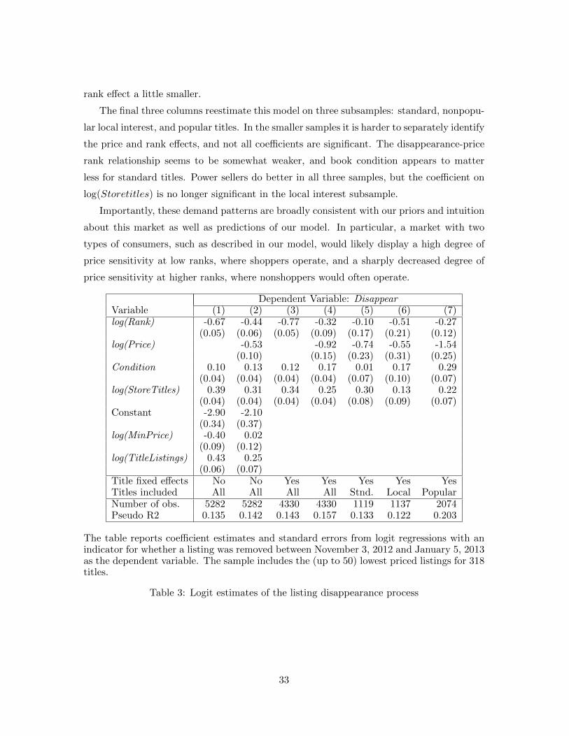
rank effect a little smaller.

The final three columns reestimate this model on three subsamples: standard, nonpopu-

lar local interest, and popular titles. In the smaller samples it is harder to separately identify

the price and rank effects, and not all coefficients are significant. The disappearance-price

rank relationship seems to be somewhat weaker, and book condition appears to matter

less for standard titles. Power sellers do better in all three samples, but the coefficient on

log(Storetitles) is no longer significant in the local interest subsample.

Importantly, these demand patterns are broadly consistent with our priors and intuition

about this market as well as predictions of our model. In particular, a market with two

types of consumers, such as described in our model, would likely display a high degree of

price sensitivity at low ranks, where shoppers operate, and a sharply decreased degree of

price sensitivity at higher ranks, where nonshoppers would often operate.

Dependent Variable: DisappearVariable (1) (2) (3) (4) (5) (6) (7)log(Rank) -0.67 -0.44 -0.77 -0.32 -0.10 -0.51 -0.27

(0.05) (0.06) (0.05) (0.09) (0.17) (0.21) (0.12)log(Price) -0.53 -0.92 -0.74 -0.55 -1.54

(0.10) (0.15) (0.23) (0.31) (0.25)Condition 0.10 0.13 0.12 0.17 0.01 0.17 0.29

(0.04) (0.04) (0.04) (0.04) (0.07) (0.10) (0.07)log(StoreTitles) 0.39 0.31 0.34 0.25 0.30 0.13 0.22

(0.04) (0.04) (0.04) (0.04) (0.08) (0.09) (0.07)Constant -2.90 -2.10

(0.34) (0.37)log(MinPrice) -0.40 0.02

(0.09) (0.12)log(TitleListings) 0.43 0.25

(0.06) (0.07)Title fixed effects No No Yes Yes Yes Yes YesTitles included All All All All Stnd. Local PopularNumber of obs. 5282 5282 4330 4330 1119 1137 2074Pseudo R2 0.135 0.142 0.143 0.157 0.133 0.122 0.203

The table reports coefficient estimates and standard errors from logit regressions with anindicator for whether a listing was removed between November 3, 2012 and January 5, 2013as the dependent variable. The sample includes the (up to 50) lowest priced listings for 318titles.

Table 3: Logit estimates of the listing disappearance process

33

5 A Structural Model of the Market

In the model we discussed earlier, online prices differ from offline prices for two offsetting

reasons: increases in consumer arrival rates and distributions of valuations tend to increase

online prices; and increased competition brings online prices down. The welfare effects

of online sales depend on the magnitudes of the underlying gross effects: the increase in

consumer arrival rates; the increase in consumer valuations; the equilibrium delay before

sales occur; etc. In this section we develop and estimate a structural model which includes

all of these effects. We note that features of the model make it amenable to estimation

via simulated maximum likelihood. Our estimates indicate that customer arrival rates

were substantially higher online than offline by 2009 and suggest that Internet sales led to

substantial increases in both profits and consumer surplus.

5.1 A structural framework

In this section we discuss an empirical model closely related to that discussed in our theory

section and note that aspects of the model facilitate estimation.

Consider a model similar to that of section 2 in which I + 1 populations of consumers

shop for each title k at stores i = 1, 2, . . . , I.24 One of these is a population of shoppers

who arrive at Poisson rate γ0k. Shoppers observe all prices and purchase from store i at

the instant at which they arrive with probability Dok(pik, p−ik;Xik,Λ, βik), where Xik is a

vector of characteristics of store i and title k, Λ is a vector of parameters to be estimated,

and βik is a vector of unobserved random coefficients. Assume that the arrival rate γ0k

and random coefficient vector βik are draws from distributions that may depend on the

parameter vector Λ.

The other I populations are nonshoppers who do not compare prices across sellers:

nonshoppers from population i arrive at store i at Poisson rate γik. Suppose that they

purchase upon arrival with probability Dmik(pi;Xik,Λ, βik). Again, the γik and βik are

random variables with a distribution that may depend on Λ.

Assume that stores choose the prices that would maximize expected profits in a sta-

tionary dynamic model like that of section 2, i.e. assume that pik is chosen to maximize

πi(pik, p−ik) ≡pik(γikD

mk (pi) + γ0kD

ok(pik, p−ik))

r + γikDmk (pik) + γ0kD

ok(pik, p−ik)

,

where we have omitted the characteristics and parameters from the arguments for readabil-

ity.

24The number of sellers varies by title, but we omit the k subscript on I in this description for simplicity.

34

Suppose that we are given data on a set of titles k = 1, 2, ..., . . . ,K. These data will take

two distinct forms. For some titles we observe just the vector of prices (p1k, p2k, . . . , pIk).

For other titles we observe both prices and an indicator for whether the title sells in a given

time period: (p1k, q1k, . . . , pIk, qIk). We wish to estimate the parameter vector Λ.

One observation about this model that will facilitate estimation is that the first order

condition for store i’s title k price to be optimal,

0 = rpikγikDm ′(pik) + rγikD

m(pik) + γ2ikD

m(pik)2

+rpikγ0k∂Do

∂pi(pik, p−ik) + rγ0kD

o(pik, p−ik) + γ20kD

o(pik, p−ik)2

+2γ0kγikDm(pik)D

o(pik, p−ik),

is a quadratic function of γik once one fixes γ0k, the parameters affecting Dm(pik), and

Do(pik, p−ik), and values for the random coefficients. Specifically, this FOC is of the form

aγ2ik + bγik + c = 0 for

a(pik, Xik; Λ, βik) = Dm(pik)2

b(pik, Xik; Λ, βik) = rpikDm ′(pik) + rDm(pik) + 2γ0kD

m(pik)Do(pik, p−ik)

c(pik, Xik; Λ, βik) = rpikγ0k∂Do

∂pi(pik, p−ik) + rγ0kD

o(pik, p−ik) + γ20kD

o(pik, p−ik)2

Under some conditions (b > 0, c < 0), only the larger root of this quadratic will be positive.

When this occurs, we can calculate the conditional likelihood of each price observation pik

(conditional on the parameters, Xik, and random coefficients) by backing out the unique

γik which makes pik optimal and then computing the likelihood via

L(pik|γ0k, Xik,Λ, βik) = L(γik|γ0k, Xik,Λ, βik)1

∂g∂γ (γik)

,

where g is the best-response pricing function with g(γik) = pik. By implicitly differentiating

the FOC we find that

∂g

∂γik(γik) = − 2γika(pik) + b(pik)

∂a∂pik

γ2ik + ∂b

∂pikγik + ∂c

∂pik

.

Another aspect of our model that facilitates estimation is that the one-to-one corre-

spondence between the observed pik and unobserved γik also makes it easy to account for

endogeneity when using the demand data. Given the observed pik and an inferred γik, the

“net” arrival rate of consumers who would buy book k from store i is

dik ≡ γ0kDo(pik, p−ik) + γikD

m(pik)

35

Hence the probabilty that the book will be sold in a ∆t time interval is

E(qik|pik, p−ik, γ0k,Λ, βik) = 1− edik∆t.

The joint likelihood of observed pairs (pik, qik) is simply the product of this expression and

our earlier expression for the likelihood of pik.

Together these two observations suggest a simple procedure for simulated maximum

likelihood estimation. Given any potential parameter vector Λ, we take random draws

for any random coefficients (which may vary by title or by listing). Given these random

coefficients, we compute the joint likelihood of each observed price vector (p1k, . . . , pIk)

and of each observed price/quantity vector (p1k, q1k, . . . , pIk, qIk) using the above formulae.

Summing across the draws of the random coefficients gives the unconditional likelihood.

Parameter estimates are obtained by maximizing this likelihood over the parameter space.

5.2 Empirical specification

To estimate arrival rates and demand in the used book market and explore how they have

changed with the shift to online sales, we implement a parsimonious version of the model

including only as many parameters and random coefficients as was necessary to estimate

quantities of interest and match the main features of the data.

We assume that the arrival rate of shoppers varies only with the “popularity” of a title

and the year (2009 versus 2012):

γ0k = γ0PopularityγN0k ∆γ

2012 I(t=2012)0 .

The Popularityk variable is the ratio between the count of listings for title k in the 2012

online data and the mean of this count across listings. We assume that shoppers have

logit-style preferences: consumer j is gets utility

uijk =

XkΛ− αδkpik + εijk if j purchases title k from store iXkΛ + β0k + εijk if j does not purchase title k

,

where the εijk are independent random variables with a type 1 extreme value distribution.

The demand for firm i’s offering is then

Dok(pik; p−ik) =

e−αδkpik

eβ0k +∑

` e−αδkp`k

.

The parameters δk let the price-sensitivity vary across titles, which will help the model fit

data in which price levels vary substantially across titles. We will adopt a random coeffi-

cients specification which allows the unobserved outside good utilities β0k to be normally

36

distributed across titles. This feature helps to fit data in which the fraction of listings

that sell varies substantially across titles and also helps the model explain why one store

sometimes substantially undercuts all other stores.

The arrival rate of nonshoppers is similarly allowed to vary with popularity, year, and

whether a store is online/offine. We assume that it also varies randomly across store-titles

– a store’s price is an increasing function of the rate at which it is visited by nonshoppers,

and it is through the random variation in γik that the model can account for each observed

price as a best response. Formally, the arrival rate is

γik = zikPopularityγNik ∆γ

2012 I(t=2012)i ∆γ

off I(offline)i ,

where the zik are i.i.d. gamma-distributed random variables with mean µγi and standard

deviation σγi . We assume that nonshopper demand curves have the constant elasticity

form. In utility terms, this amounts to assuming that a nonshopper j considering buying

book k from store i gets utility

uikj =

vj − δkpik if he buys.0 if he does not

,

where the vj are heterogeneous across consumers with density f(vj) = hηv−η−1 on [h1/η,∞].

We assume that η > 1 (otherwise the monopoly price is infinite) and that h > 0 is sufficiently

small so that all observed prices are in the support of the value distribution. With this

assumption the probability that a shopper purchases at the observed price is

Dm(pik) = h(δikpik)−η.

The model description above has more parameters than we are able to estimate. There

are two issues of identification: the arrival rate γik of nonshoppers cannot be separately

identified from the multiplicative constant h in nonshopper demand; and all profit functions

only depend on ratios γ/r. Also, as a practical matter, we are unable to estimate the large

number of title fixed effects δk that shift the level of equilibrium prices for each title.

Accordingly, we have chosen to fix some parameters in our estimation. We fix r = 0.05 so

that arrival rates should be thought of as arrivals over a period of one year. We set the

constant h in the shopper demand equation to one.25 And, finally, we implicitly fix the δk

25We treat demand as being p−η even when this expression is greater than one and hence inconsistentwith the demand being a probability of purchase given arrival. Note, however, that the same equationscould always have be made consistent with the probability interpretation simply by choosing a smaller valueof h and scaling up the consumer arrival rate while keeping their product constant.

37

at a different value for each book by scaling the prices for each book so that the lowest 2009

online price is equal to one and then setting each δk to one.

These assumptions produce a model with twelve parameters to be estimated: (γ0,∆γ20120 ,

γN0 , α, µβ, σβ, µγi , σγi ,∆γ2012i , γNi , η,∆γ

offi ). We estimate these parameters on a dataset

containing 313 books which had valid listings in all four of our data collection waves: they

were found in an offline store in 2009 and had listings successfully scraped from Abe-

Books.com in all three online collections.26 The demand data qik are inferred by comparing

the November 2012 and January 2013 listings, and are used only for books for which our

2013 data collection was complete. The estimation follows the procedure noted above with

the “outside options” β0k as the only random coefficients.27

5.3 Estimates of arrival rates and demand

Table 4 presents estimates of the parameters of our structural model. The left half of the

table reports estimates related to the nonshoppers. The most basic finding is that the

“net” arrival rate of nonshoppers (arrival rate of a nonshopper who actually purchases) at

online stores appears to be quite low. The µγi = 0.054 estimate indicates a firm with a

typical listing should expect that a nonshopper willing to purchase the good at the lowest

price in 2009 online data for that title will arrive approximately once every 18.5 years.

The σγi = 0.04 estimate indicates that there is variation across stores, with some having

essentially no nonshoppers and others having substantially more. The γNi = 0.14 estimate

indicates that arrival rates are higher for more popular titles, but it is not a very big

effect. For example, a title that has twice as many listings as average has about a ten

percent higher (per listing) arrival rate of nonshoppers. The year dummy indicates that

nonshopper arrival rates did not change between 2009 and 2012. All of these estimates

are fairly precise. Intuitively, the 2012 quantity observations for high-priced firms provide

a lot of information about nonshopper arrival rates, and the fact that the upper parts of

the price distributions are so similar in 2009 and 2012 drives the estimate that nonshopper

arrival rates must be similar in the two years.

26For our structural analysis we also drop all listings priced above $50 and any title that does not haveat least two listings.

27With just one random coefficient relevant to each title, the “simulated” maximum likelihood becomesjust a numerical integration over the unknown coefficient. We perform this integration by evaluating thelikelihood for 50 values of the random coefficient spaced evenly in CDF space. For some parameters the modelcannot rationalize some observations (in which one firm sets a price substantially below the second lowest

price) using any positive γik). When this happens we use a penalty function, L(pik|Xik,Λ) = e−10+10|γik|

that increases in the distance between the (negative) γik that would make the first-order condition forprofit-maximization satisfied and the nearest value that is in the support of the distribution (which is zero).

38

Parameter Coef.Est. SE Parameter Coef.Est. SENonshopper arrival Shopper arrival

µγi 0.054 (0.003) ln(γ0) 3.70 (2.68)σγi 0.04 (0.003) ∆γ2012

0 1.06 (0.49)∆γ2012

i 1.02 (0.04) γN0 1.23 (0.20)γNi 0.14 (0.02)

Offline arrival 2009 Shopper utility

∆γoffi 0.36 (0.03) µβ -8.21 (2.31)

Nonshopper utility σβ 3.80 (0.34)η 1.15 (0.01) α 13.34 (1.42)

Table 4: Estimates of structural model parameters

Although nonshopper arrival rates at online stores are modest, the coefficient directly

below this indicates that they are still substantially higher than arrival rates at offline

stores. The 0.36 estimate for ∆γoffi indicates that 2009 offline arrival rates were only about

36% of online arrival rates, or about 0.02 consumers per year for the typical listing.28 Such

a difference in arrival rates would lead to substantial differences in the expected welfare

gains produced by an eventual sale. Of course, it should be kept in mind that, unlike in the

online world, these arrival rates are estimated without any quantity data and instead reflect

just that lower offline prices can be rationalized in our model only by a lower consumer

arrival rate. Despite that caveat, we do not find it at all implausible that a lot of used

books sat on the shelves of used book dealers for years waiting for an interested buyer to

happen by.

The final estimate on the left side is an estimate of the elasticity of demand of the

nonshoppers. The estimated elasticity of demand is -1.15. A constant elasticity demand

curve with this elasticity has a very thick upper tail. Such a situation will lead to estimates

that each sale to a nonshopper generates a great deal of consumer surplus.

The right half of the table reports estimates related to the population of online shoppers.

When interpreting arrival rates, keep in mind that “net arrival rates” will be lower than the

arrival rate coefficient because some consumers prefer the outside good. We have allowed

for unobserved heterogeneity across titles in the net shopper arrival rate by introducing

heterogeneity in the utility of the outside option. The estimated mean outside good utility

turns out to be substantially higher than the mean utility provided by the lowest-priced

listing for each title, so for the median title, only a little over 1% of arriving shoppers will

28Note, however, that prices and demand are scaled so that a potential consumer buys with probabilityone if he sees a price equal to the lowest 2009 online price. Offline firms that set lower prices will sell at asomewhat higher probability.

39

actually purchase from anyone. The estimated variance of the outside good utility indicates

that there is a great deal of unobserved heterogeneity across titles. About 9% of titles have

outside good utilities that are below the mean utility provided by the lowest-priced listing,

in which case most shoppers will purchase. At the other extreme, a large number of titles

have essentially no shoppers willing to purchase at the observed prices.

The estimated shopper arrival coefficient (e3.70 ≈ 40) indicates that some titles of will

have a net arrival rate of nearly 40 consumers per year.29 This is dramatically higher than

the rate at which nonshoppers are estimated to arrive. As noted earlier, however, it is

only a few titles that have such shopper net arrival rates. The median title is estimated to

have a shopper net arrival rate that is comparable to each firm’s nonshopper arrival rate,

and other titles are estimated to have very few shoppers at all. These estimates reflect

a basic fact about demand noted earlier: we observe many sales of some titles, but zero

sales over a two-month period for about one-third of the titles in our sample. Note also

that the standard error on the estimate of ln(γ0) is very large. This reflects a collinearity

between the arrival rate and the outside good utility – it is hard to tell whether there is a

large arrival rate of consumers who are each unlikely to purchase or a lower arrival rate of

consumers who are each likely to purchase.

The γ0N = 1.23 estimate indicates that the number of shoppers increases more than

proportionately to a title’s popularity. Note that the fraction of consumers who are shoppers

is roughly independent of popularity because the coefficient estimate for nonshoppers is for

a single store, whereas the coefficient estimate for shoppers is for the whole population.

The estimates do imply, though, that the potential benefit of attracting shoppers is a more

important consideration for stores selling popular titles.

Unfortunately, we are unable to say much about how Amazon’s incorporation of Abe-

Books’s listings affected the shopper arrival rate. The imprecise estimate of ∆γ20120 indicates

an increase of arrivals of 6%±49%. Hence, the 95% confidence interval includes both a dou-

bling of the shopper arrival rate and substantial decreases. We can reject larger increases

in the shopper arrival rate.

The price coefficient α = 13.34 indicates that online shoppers are very price sensitive.

In most cases (excluding, for example, when the “outside option” is unusually bad), this

estimate implies that a firm with a price close to the lowest listed price will see its demand

go down by about 13% if it raises its price by 1%. A consequence of this price sensitivity

29In this paragraph we use “net arrival rate” to refer to the arrival rate of shoppers willing to purchasefrom a store offering the lowest price observed in the data for that title.

40

coupled with our logit functional form assumption is that a standard welfare calculation

will indicate that shoppers who purchase the book do not get a great deal of consumer

surplus. In principle, one could avoid this implication by putting heterogeneity directly into

the the shopper arrival rate and estimating a more flexible demand function that allowed

consumers to have different price sensitivities among inside goods versus the outside good.

But in practice, our data do not make it possible to estimate such a flexible specification.

5.4 Estimating welfare gains

In this section we examine both welfare gains from a shift from offline to online used

book sales and the division of these gains between consumers and stores. Welfare gains

occur when books are sold to consumers with higher valuations and/or books are sold

more quickly. Online retailers must be better off if the number of nonshoppers (and the

distribution of their valuations) increases, but the magnitude of the gain will be affected by

the size of these increases and the relative sizes of the shopper and nonshopper populations.

Given an estimated parameter vector Λ, the average per-listing welfare generated by

the listings for title k can be calculated by integrating over the posterior distribution of the

unobserved random coefficient β0k:

E(Wk|Λ) =1

Ik

∫β

(E(CSk|Λ, β) +

∑i

E(π(pik, p−ik)|Λ, β)

)f(β|p1k, . . . , qnkdβ,

where Ik is the number of listings for title k, CSk, is the total discounted consumer surplus

generated by the eventual sales of all the listings and π is the discounted expected profit

that the firm listing copy i will earn.

The profit term can be computed using the same profit functions we use in estimating

the model. Given the price pik, a value β0k for the outside good utility, and the other

estimated parameters, we back out a value for γik. Expected profits are then simply

E(π(pik, p−ik|Λ, β) =pik(γikD

m(pik) + γ0kDo(pik, p−ik))

r + γikDm(pik) + γ0kDo(pik, p−ik)

Consumer surplus is a little more complicated. It is a sum of consumer surplus from

sales to nonshoppers and sales to shoppers. The two are most naturally calculated in dif-

ferent ways. Expected total consumer surplus from sales to nonshoppers can be calculated

similarly to how we calculated profits:

E(CSnsk ) =∑i

E(e−rti)Probi sells to a nonshopperE(v − pik|v > pik)

=∑i

γikDm(pik) + γ0kD

o(pik, p−ik)

r + γikDm(pik) + γ0kDo(pik, p−ik)

γikDm(pik)

γikDm(pik) + γ0kDo(pik, p−ik)

pikη − 1

.

41

The consumer surplus that accrues to shoppers, on the other hand, is easier to calculate

by thinking about the present value of the flow consumer surplus that accrues as shoppers

arrive because consumers prefer choosing among the Ik goods at the observed prices to

being forced to buy the outside good:

E(CSsk) =

∫ ∞0

γ0k(E(CS(p1k, . . . , pIkk)− E(CS(∞, . . . ,∞))e−rtdt

=γ0k

r

1

α

(log(eβ +

∑i

e−αpik)− β

).

The final step here takes advantage of the well known formula for the logit inclusive value to

calculate how the expected consumer surplus of each shopper increases due to the presence

of the inside goods.

Recall that in the case of isoelastic demand and no shoppers, expected welfare will

simply be the price, but these formulae tell us how this welfare is divided. They are also

more general, applying the cases with arbitrary demand and shoppers.

5.5 Welfare gains from Internet sales

In this section we present profit and welfare estimates calculated using the above methodol-

ogy. Among our main findings are that profits and consumer surplus resulting from online

sales are quite large and represent a substantial gain to market participants relative to the

offline market for used books. An increase in the number of listings between 2009 and 2012

may have lead to an additional welfare increase, although per-listing profits are estimated

to have declined somewhat from the 2009 level.

The first row of Table 5 presents estimates of the expected gross profit per listing. More

precisely, it is the average across titles of the average across listings of the estimated gross

profit given the listing’s price and our estimated demand parameters. We use the 313 titles

that have valid listing in both 2009 and 2012. (These are “gross” profits in that they do not

account for the acquisition cost of the books being sold.) A first finding, visible in the first

column, is that average per-listing profits are estimated to have been fairly low in the offline

world, just $1.32 per listing. This is the product of the mean price for the titles, $10.21,

and a discount factor of E(e−0.05t), reflecting the fact that sales occur probabilistically in

the future. In particular, the estimated discount factor of 0.13 reflects our estimates that

many books would take decades to sell: offline arrival rates are about 0.02 customers per

year. The second column gives comparable figures for the 2009 online listings. It illustrates

the dramatic increase in profits from moving online: per listing gross profits are estimated

42

to be over twice as large at $3.11. The higher gross profits reflect both higher average prices

and a higher estimated sales rate, which reduces the extent to which the eventual sales are

discounted. Note, however, that the three-times higher arrival rate does not reduce the

effective discount factor as much as a naive calculation would indicate: firms react to the

higher arrival rate by increasing prices, and high-priced listings take longer to sell. The

final column presents estimates for the 2012 listings. The estimates indicate that per-listing

profits are still well above the 2009 offline profit level, although not as high as the 2009

online profits. This reflects both that average prices and price-weighted waiting times to

sell are intermediate. The waiting time effect reflects the model’s prediction that for many

titles, high priced firms are now very unlikely to sell to a shopper.

Average value 2009 offline 2009 online 2012 onlineper listing listings listings listings

Gross profit $1.32 $3.11 $2.29(0.07) (0.10) (0.10)

Price × $10.21 $15.04 $13.80Discounting × 0.13 × 0.21 × 0.17

Consumer surplus $8.90 $16.61 $13.63(0.09) (0.85) (0.50)

Nonshoppers + $8.85 $16.01 $13.36Shoppers + $0.60 + $0.27

Welfare $10.21 $19.73 $15.91(——) (0.87) (0.49)

Table 5: Profit and welfare estimates

In thinking about the reliability of these estimates, it should be noted that the 2012

figures are estimated from better data – it is only in 2012 that we have a proxy for the rate

at which listings are sold. The 2009 vs. 2012 online comparison reflects both the observed

fact that average online prices were higher (recall that price distributions were otherwise

similar but 2012 had more low-priced listings), and the structural model’s inferences about

demand: the similar upper tails suggest that nonshopper arrival rates were similar in 2009,

and the demand model infers that the growth of low-priced listings would have reduced

the number of sales that high-priced firms make to shoppers. Also, the 2009 offline profit

estimates are made without the sales proxy as well. We know prices were lower but are

43

relying on the model’s inference that firms set lower prices because they were facing lower

demand.

The second row of the table presents estimates of consumer surplus. Here, the estimates

indicate that consumers also benefitted substantially from the shift to online sales. In 2009

online listings are estimated to generate, on average, almost twice the consumer surplus

(per listing) as offline listings. As noted in the introduction, the naive intuition that higher

online prices suggest that consumers are not benefitting from online sales misses the basic

point that profits and consumer surplus can both be higher if Internet sales result in higher

match quality and faster sales. The estimates indicate that this is true to an extreme:

consumers are estimated to capture most of the total surplus generated by both online and

offline sales, and in 2009 consumer surplus per listing is estimated to be almost twice as

high for online sales.

The estimates that consumer surplus is so much higher than profits reflects the distribu-

tion of prices. The model rationalizes the coexistence of low and high prices via a demand

curve with a very thick upper tail, which then makes the average valuation of consumers

who purchase very high. The thickness of the uppermost part of the tail, of course, relies

on functional form assumptions, and one could also worry that some high prices are not

actually profit-maximizing. For this reason, the precise magnitudes here should be taken

with a grain of salt. Another limitation of our model, mentioned earlier, however, works in

the other direction. In assuming a simple logit specification for demand, we have assumed

that consumers who are very price-sensitive when comparing online listings are equally price

sensitive in comparing listings to the outside option of not purchasing. This feature biases

us towards a finding of relatively little consumer surplus. Although it would be preferable

to estimate a model with more flexible substitution patterns, such as a nested logit model

with the outside good in a separate nest if it were feasible, we are perhaps fortunate that

these biases work in opposite directions.

The third row of the table presents estimates of total welfare. Our model of 2009

offline sales is a version of the monopoly-constant elasticity model discussed in section 2.1.

As a result, the estimated welfare is simply the average price (and is independent of the

estimated parameters). Our empirical models for the 2009 and 2012 online markets are not

just monopoly models, so the welfare estimates will depend on the estimated parameters.

The estimates are that per-listing welfare was almost twice as high in the 2009 online market

as in the 2009 offline market. Welfare is somewhat lower in 2012 than 2009 reflecting the

increased sales to nonshoppers and the somewhat lower prices.

44

6 Conclusion

A number of previous studies have noted that the Internet has not transformed retail

markets as some forecast: price declines have been more moderate than revolutionary, and

the “law of one price” has not come to pass. We began this paper by noting that the

Internet market for used books shows these effects in the extreme: prices increased in a

strong sense and there is tremendous price dispersion. We feel that these facts make the

Internet market for used books a nice environment in which to try to gain insight into the

mechanisms through which the Internet affects retail markets. Crucially, we emphasized

that these basic facts do not necessarily indicate that the Internet has failed to live up

to its promise. If Internet search allows consumers to find products that are much better

matched to their tastes, then it leads to an increase in demand which can lead to higher

prices in a variety of models (particularly for goods like out-of-print books for which supply

is fairly inelastic).

The match-quality-increased-demand theory is very simple, so to provide evidence in

its favor we devoted a substantial part of our paper to developing less obvious implications

that could be examined to help assess its relevance. We examined these implications using

three sources of variation. First, we examined how price distributions – rather than just

price levels – differ between the online and offline markets. Here, our primary supporting

observation was that the online price distribution for standard titles has a thick upper

tail where the offline distribution had none. Second, we examined how price distributions

differed for different types of used books. Here, we noted that price increases were smaller

for popular books (which one would expect if the valuation distribution had less of an upper

tail and there is more competition) and that there was already an upper tail of prices for

local interest books in physical bookstores. One of our favorite characterizations of the

latter result is that it appears as if the Internet has made all books of local interest. Third,

we examined how online price distributions changed between 2009 and 2012. Here, we noted

that the Amazon-induced increase in viewing of aggregated listings would be expected to

increase the number of sellers offering very low prices but have little impact on the upper

part of the price distribution, and found that this was strikingly true in the data. Our

demand analysis also revealed patterns that seem consistent with the assumptions of our

model: there is a concentration of demand among the top-ranked firms as one would expect

from a price-senstive shopper segment; but firms with much higher prices also appear to

have some probability of making a sale.

45

The structure of our model – in particular the use of one-dimensional unobserved het-

erogeneity and the assumption that firms maximize relative to steady-state beliefs – makes

it relatively easy to estimate structurally. The one-to-one mapping between unobserved

consumer arrival rates and observed prices makes it easy to control for endogeneity in de-

mand and to estimate the model via simulated maximum likelihood. And consumer surplus

and welfare are easily calculated from the estimated parameters by computing some things

on a title-by-title basis and others on a consumer-by-consumer basis. Our implementation

of the model suggests that there were substantial increases in both profits and consumer

surplus from the move to online sales of used books. Amazon’s subsequent incorporation of

used-book listings seems to have reduced book dealer profits somewhat, but they are still

much higher than they were in the offline world.

Our analysis has a number of limitations that could provide opportunities for future

research. On the theory side it would be interesting to analyze a similar dynamic pricing

problem without the steady-state beliefs we have imposed in the model: there could be

interesting swings in pricing as duopolists hold off on selling in hopes of becoming a mo-

nopolist and then lower prices substantially when entry occurs and makes this less likely.

On the empirical side we think that the combination of assumptions we have used could

make other analyses tractable as well, but think that it would also be worth exploring gen-

eralizing our model in other ways and allowing for multidimensional heterogeneity among

firms. With regard to used books, we think that among the most important elements we

have not incorporated is a relation between market prices and the flow of used books into

used book dealers. Building out the model in this direction would also be useful for un-

derstanding differences in how different retail markets have been affected by the Internet

growth.

46

References

Arrow, Kenneth J., Theodore Harris, and Jacob Marschak (1951): “Optimal Inventory

Policy,” Econometrica 19, 250-272.

Baye, Michael R., and John Morgan (2001): “Information Gatekeepers on the Internet and

the Competitiveness of Homogeneous Product Markets,” American Economic Review 91,

454-474.

Baye, Michael R., John Morgan, and Patrick Scholten (2004): “Price Dispersion in the

Small and the Large: Evidence from an Internet Price Comparison Site,” Journal of Indus-

trial Economics 52, 463-496.

Baye, Michael R., John Morgan, and Patrick Scholten (2006): “Information, Search, and

Price Dispersion,” in Terence Hendershott (ed.) Handbook on Economics and Information

Systems. Amsterdam: Elsevier.

Brown, Jeffrey R., and Austan Goolsbee (2002): “Does the Internet Make Markets More

Competitive? Evidence from the Life Insurance Industry,” Journal of Political Economy

110, 481-507.

Brynjolfsson, Eric, Yu Jeffrey Hu, and Michael D. Smith (2003): “Consumer Surplus in

the Digital Economy: Estimating the Value of Increased Product Variety at Online Book-

sellers,” Management Science 49, 1580-1596.

Burdett, Kenneth and Kenneth L. Judd (1983): “Equilibrium Price Dispersion,” Econo-

metrica, 51, 955-969.

Butters, Gerard (1977): “Equilibrium Distributions of Sales and Advertising Prices,” Re-

view of Economic Studies, 44, 465-491.

Chevalier, Judith, and Austan Goolsbee (2003): “Measuring Prices and Price Competition

Online: Amazon vs. Barnes and Noble,” Quantitative Marketing and Economics 1, 203-222.

Clay, Karen, Ramayya Krishnan, and Eric Wolff (2001): “Prices and Price Dispersion on

the Web: Evidence from the Online Book Industry,” Journal of Industrial Economics 49,

521-539.

De los Santos, Babur, Ali Hortacsu, and Matthijs R. Wildenbeest (2012): “Testing Models

47

of Consumer Search Behavior Using Data on Web Browsing and Consumer Purchases,”

American Economic Review, 102(6), 2955-2980.

Ellison, Glenn (2005): “A Model of Add-on Pricing,” Quarterly Journal of Economics,

120(2), 585-637.

Ellison, Glenn, and Sara Fisher Ellison (2009): “Search, Obfuscation, and Price Elasticities

on the Internet,” Econometrica, 77(2), 427-452. 10570.

Hortacsu, Ali, and Chad Syverson (2004): “Product Differentiation, Search Costs, and

Competition in the Mutual Fund Industry,” Quarterly Journal of Economics 119, 403-456.

Hong, Han, and Matthew Shum (2006): “Using Price Distributions to Estimate Search

Costs,” RAND Journal of Economics 37 (2), 257-275.

Karlin, Samuel (1962): “Stochastic Models and Optimal Policy for Selling an Asset,” in

Kenneth J. Arrow, Samuel Karlin, and Herbert Scarf (eds.) Studies in Applied Probability

and Management Science. Stanford: Stanford University Press.

Kim, Jun B., Paulo Albuquerque, and Bart J. Bronnenberg (2010): “Online Demand Under

Limited Consumer Search,” Marketing Science 29, 1001-1023.

Koulayev, Sergei (2013): “Estimating Demand in Search Markets: the Case of Online Hotel

Bookings,” Rand Journal of Economics, forthcoming.

McCall, J. J. (1970): “Economics of Information and Job Search,” Quarterly Journal of

Economics 84, 113-126.

Moraga Gonzalez, Jose Luis, and Matthijs R. Wildenbeest (2008): “Maximum Likelihood

Estimation of Search Costs,” European Economic Review 52, 820-848.

Moraga Gonzalez, Jose Luis, Zsolt Sandor, and Matthijs R. Wildenbeest (2013): “Semi-

Nonparametric Estimation fo Consumer Search Costs,” Journal of Applied Econometrics,

forthcoming.

Reinganum, Jennifer (1979): “A Simple Model of Equilibrium Price Dispersion,” Journal

of Political Economy, 87, 851-858.

Salop, Stephen and Joseph Stiglitz (1977): “Bargains and Ripoffs: A Model of Monopolis-

tically Competitive Price Dispersion,” Review of Economics Studies, 49, 3-13.

48

Smith, Michael D. and Erik Brynjolfsson (2001): “Consumer Decision-Making at an Inter-

net Shopbot: Brand Still Matters,” Journal of Industrial Economics 49, 541-558.

Stahl, Dale O. (1989): “Oligopolistic Pricing with Sequential Consumer Search,” American

Economic Review 79, 700-712.

Varian, Hal (1980): “A Model of Sales,” American Economic Review, 70, 651-659.

49

Superbowl Ads∗

Wesley R. Hartmann Daniel Klapper

Graduate School of Business School of Business & Economics

Stanford University Humboldt University Berlin

June, 2014

First Draft: June, 2012

Abstract

We explore the eects of television advertising in the setting of the NFL's Super Bowl telecast.The Super Bowl is the largest advertising event of the year and is well suited for measurement. Theevent has the potential to create signicant increases in brand capital because ratings averageover 40 percent of households and ads are a focal point of the broadcast. Furthermore, variationin exposures is exogenous because a brand cannot choose how many impressions it receives in eachmarket. Viewership is determined based on local preferences for watching the two competing teams.With this signicant and exogenous variation in Super Bowl advertising exposures we test whetheradvertisers' sales are aected accordingly. We run our analysis using Nielsen ratings and storelevel sales data in the beer and soda categories. We nd that Super Bowl ads generate signicantincreases in revenue and volume per household. However, when two major brands both advertise,they erode most of the gain. The largest eects occur during weeks with spikes in other sportsevents suggesting that placing an advertisement in the most watched sporting event of the yeargenerates associations with sports more broadly. We test this using local viewership data of NCAAbasketball in the second month after the Super Bowl and nd strong evidence that advertising cangenerate or augment complementarities between a brand and the ways potential consumers spendtheir time.

Keywords: advertising, television, complements.

∗Email addresses are hartmann_wesley@gsb.stanford.edu and daniel.klapper@hu-berlin.de. The authors would like tothank Lanier Benkard, Latika Chaudhary, Brett Gordon, Jesse Shapiro, Ken Wilbur, seminar participants at UC Davisand Michigan, conference participants at the 2012 Marketing Science Conference, the 5th Workshop on the Economicsof Advertising and Marketing in Beijing, and the 2013 Summer Institute in Competitive Strategy. Corey Anderson andChris Lion provided valuable research assistance on this project. An early version of this paper circulated under thetitle Do Super Bowl Advertisements Aect Brand Shares? and documented null eects for share regressions. Ourconclusions changed as we considered additional specications and data.

1

1 Introduction

The Super Bowl is the premier advertising event of the year. Four of the ve most watched telecasts

ever were Super Bowls. The 2012 broadcast was the most watched telecast in history at 54% of US

households. Costs of airing a thirty second spot during the game have grown to more than $3 million.

Two of the biggest Super Bowl spenders have been Anheuser-Busch (Budweiser) and Pepsi1: both

well-known brands whose existence and tastes presumably do not need to be communicated. This

highlights one of the most puzzling questions in advertising: Can continued heavy advertising by

established brands pay o, and if so why?

The eectiveness of most television advertising is dicult to gauge because media planners try

to concentrate exposures to the best potential targets. This creates an obvious correlation between

advertising and sales that confounds attempts to infer causality. The Super Bowl presents a very inter-

esting laboratory to study TV ad eectiveness because brands cannot control how many exposures

they receive in a given market. It is driven by preferences to watch the two competing teams. For

example, when the Green Bay Packers returned to the Super Bowl after 13 years in 2011, ratings

increased by 14 points in Milwaukee. That exposed more Wisconsinites and Packers fans elsewhere to

perennial advertisers. If those ads are eective, we should see perennial Super Bowl advertisers exhibit

a corresponding increase in their sales. We nd exactly this. Analyzing weekly market level sales of

beer and soda over the 2006-2011 time period, a ten point increase in Super Bowl viewership increases

advertisers' revenue by 1 to 3.5 percent in the two months following the game.

We also nd Super Bowl advertising to increase consumption during other sporting events. In

the soda category, the eect of Coke and Pepsi Super Bowl ads spikes up during events such as the

beginning of the NCAA basketball tournament, its Final Four, the Major League Baseball season, and

the NBA Playos and Finals. To test the validity of this link, we collect market-week level viewership

data for the NCAA basketball tournament and interact it with the Super Bowl ad viewership. We nd

that the Super Bowl advertiser outperforms its competitor the most when local viewership of both the

Super Bowl and the NCAA basketball tournament is highest. This eect is also strong in the beer

category, but is insignicant. We suspect this is because Budweiser's 20 years as the exclusive advertiser

1http://sports.espn.go.com/n/news/story?id=4751415

2

may have already established its links with sports. This is evident in that Budweiser outperforms its

competitors when consumers purchase beer in the week leading up to the Super Bowl.

These ndings suggest that advertising can create a complementarity between a brand and potential

consumption occasions. It is useful to contrast this with the current view of complements in advertising.

Becker and Murphy (1993) propose advertisements themselves complement consumption. Their notion

is consistent with psychological views that the personality or cultural references in a brand's ads can

enhance the utility of consumption for people trying to embody those traits (e.g. Aaker, 1997). Our

nding is that the advertising establishes a complementarity with something else. The volume of

sports viewership in our society clearly suggests itself as a valuable complement. But other brands

may dierentiate by choosing other complements. For example, Corona beer associates itself with

relaxation and romance through imagery of a couple on a beach. This suggests that the same person

may want a Bud when watching a game with friends, but a Corona when with a (potential) partner. In

fact, the most recent ads for Budweiser emphasize Grabbing some Buds within many social contexts,

perhaps competing to be the beer of choice whenever a guy is with his buddies.

An interesting feature of this complementarity is that we nd it in the soda category where the

creative of the advertising rarely emphasizes sports. This suggests that the context in which the ad

aired can play an important role in generating this complementarity between the brand and the various

ways potential consumers spend their time. This has important implications for media companies

because a link between eectiveness and the context of the program or website can justify premium

pricing for advertising.

The soda category also allows us to explore the impact of two brands advertising head-to-head in the

Super Bowl. We observe both Coke and Pepsi advertise in some years. We nd that a direct competitor

wipes out nearly the entire benet associated with the ad. Thus, Super Bowl advertising appears to

have no eect when two major competitors advertise head to head. This suggests an incentive to keep

the competitors out, which could explain why Budweiser purchases exclusive rights to advertise beer.

It is useful to consider our ndings in the context of other studies of advertising and the Super

Bowl. The challenges of measuring advertising eects is nicely described in a series of papers beginning

with Lewis and Reiley (2013). Considering eld experiments for internet advertising, their primary

3

point is that eective advertising can involve very small changes in sales. But, detection of small eects

can requires a very large sample size if there is considerable variance in sales. They point out that this

same power issued led TV ad eectiveness studies to report ndings at the 80 percent condence

level (e.g. Lodish et.al. 1995). These challenges have been overcome by recent experimental studies

on direct mail advertising (Bertrand et.al. (2010) and internet advertising (Sahni, 2013), but there

is still a dearth of studies analyzing TV advertising with credible sources of exogenous variation. We

address these concerns by considering a market level analysis where millions of households' choices are

included and brand performance has been shown to exhibit little variance over time within markets

(Bronnenberg et.al., 2009).

There are also a couple papers that explore Super Bowl advertising specically. Lewis and Reiley

(2013) studies the eect of Super Bowl ads on search behavior and nds a signicant spike within

seconds of the airing. Such immediate search eects do not necessarily imply sales eects and would

include viewers' desires to either see the commercial again or follow up on something from the ad. The

only other paper tying exogenous variation in Super Bowl ad exposures to sales is Stephens-Davidowitz

et.al. (2013). They apply a modied version of our identication approach to the case of movies.2 They

nd signicant positive eects for movies released well after the Super Bowl. Eects in movies likely

represent a strong informative component in advertising which is consistent with past ndings such as

Ackerberg (2001), whereas our focus is on the eects and mechanism of advertising by familiar brands

with established advertising stocks (as in Dube, Hitsch and Manchanda, 2005, Doganoglu and Klapper,

2006, or Doraszelski and Markovich, 2007).

The remainder of the paper proceeds as follows. The next section describes the data sources.

Section 3 presents the estimates and section 4 concludes.

2 Data

We analyze the relationship between within market variation in Super Bowl ratings and within market

variation in Super Bowl advertisers' sales. The ratings data for the top 55 Designated Market Areas

(DMAs) is publicly released in some years, but was purchased from Nielsen. We also obtained access

2Given the lack of year over year performance measures in this category, and in light of the potential selection issuesdescribed above, they match each advertised movie with a movie that is nearly identical in various reported dimensions.

4

to the AdViews database to collect weekly advertising exposures for brands as well as market-level

exposures to ads during NFL broadcasts leading up to the Super Bowl. Data on store level revenue

and volume, as well as trade data (feature and display), come from the Kilts Center's Nielsen Retail

Scanner Data.3 The timeline for our analysis is therefore restricted to the 2006-2011 time frame for

which the store-level data is available.

2.1 Super Bowl Advertising and Ratings

We focus on the Super Bowl advertising by beer and soda brands. Anheuser Busch has been the exclu-

sive beer advertiser in the Super Bowl for the entire time span of our data. Pepsi ran an advertisement

in every Super Bowl in our data except 2007 and 2010. In 2007 they sponsored the half-time show

instead.4 The withdrawal from 2010 was based on a widely publicized refocus of their advertising

eorts toward a social media campaign. Coca-Cola advertised every year from 2007 to 2011, but prior

to that had not advertised since 1998. We later discuss potential concerns about selectivity in the

advertising decisions in the carbonated beverage category.

While there is little to no variation in our data regarding who advertises during a Super Bowl,

Figure 1 depicts substantial variation both across and within the top 56 DMAs5 in the exposures to

the Super Bowl ads. The bars at the bottom represent the average ratings for each DMA as measured

on the axis to the right. The average is 45.3 percent of a market viewing the Super Bowl, with cross-

market variation from 36.4 to 53.4 percent. The dots above represent the year by year deviations

from the DMA mean ratings as measured on the axis to the left. The DMAs are ordered left to right

with increasing variance in the ratings such that the DMA with the smallest variation across years

sees movement of roughly plus or minus 2.5 percent around its average ratings of 47.7 percent. Many

DMAs experience ratings dispersion of ten points or more, while the most variable DMAs experience

ratings dispersion of 17 points. Overall, this paints a picture of large swings in terms of how many

people are watching the Super Bowl and getting exposed to the ads.

3A previous version of this paper was circulated using the IRI Marketing data set described in Bronnenberg, Krugerand Mela (2008). We switched to the Nielsen data because of an exact match in the denition of the geographic regionand the ability to increase the number of DMAs in our analysis from roughly 33 to 56. The Nielsen data also allows usto include the smaller DMAs where statistical power is stretched.

4We've run our analysis also coding this up as an advertisement and while the coecients change some, the substantiveconclusion remains the same.

5We report 56 as opposed to 55 because of movement in and out of the top 55.

5

30.0

40.0

50.0

60.0

70.0

80.0

90.0

100.0

-30.0

-25.0

-20.0

-15.0

-10.0

-5.0

0.0

5.0

10.0

15.0

DMA

Aver

age

Ratin

gs

Ratin

gs D

iffer

ence

from

DM

A Av

erag

e

Figure 1: Super Bowl Ratings by DMA: Average and Year-Specic Deviations

From the advertisers' perspective, this variation in exposure is out of their control. It is based on

local variation in the preferences for watching the Super Bowl. While it is impossible to decompose all

of the factors generating viewership swings for the Super Bowl, we have tried to identify some of the

most signicant elements. Figure 2 illustrates the role of local preferences for the teams in the Super

Bowl in generating ratings. The horizontal axis represents the percentage of the people in the DMA

who liked the two teams in the Super Bowl on Facebook as of April 2013.6 The vertical axis plots

the associated ratings for the Super Bowl. The relationship is clearly non-linear with more than 45

percent of the population watching whenever at least 5 percent of the market likes the teams. Among

6While a better measure would include how many local people liked the teams before the respective Super Bowl, weare unaware of a historical source of such information that can date back to 2006.

6

those observations with less than 5 percent liking the team, there is still a correlation of 0.33 with the

observed ratings.

This certainly does not explain all of the variation in ratings, as Facebook is not demographically

representative and we should ideally have these preference measures at the beginning of our data. To

quantify the explanatory power, we ran a simple regression of log ratings on the log of the percent

of the DMA liking the team. The R-squared is 0.24. Including both DMA and year xed eects, we

nd that the percent liking the team explains 20 percent of the within-DMA variation in ratings. The

remainder of the variation may arise from other unobserved components of the local preferences for

the game. Some of that variation occurs because we often measure likability of the teams well after

the game was actually played. For these reasons, we choose not to use the likeability measure as an

instrument for ratings. It is a weak instrument such that we nd the standard errors on results to

increase substantially. The instrument could have been valuable to account for measurement errors7,

but is not necessary for inference as the remaining variation is unlikely to be driven by local variation

in the relative preferences of say Bud vs. Miller or Coke vs. Pepsi.

7We tested for measurement errors by allowing coecients to be interacted with number of households in the market.Smaller markets in the data should exhibit more measurement error as there are fewer local Nielsen panelists to formthe share of household viewership numbers. We did not nd this to eect the results.

7

30

35

40

45

50

55

60

0 5 10 15 20 25 30 35

Perc

ent o

f DM

A th

at W

atch

ed th

e Su

per

Bow

l

Percent of DMA that "Likes" Super Bowl teams on Facebook

Figure 2: Super Bowl Ratings by DMA: Average and Year-Specic Deviations

2.2 Retail Scanner Data

Nielsen's retail scanner data provides unit sales, prices, display and feature information at the UPC

level for each store and week. While the UPCs can be aggregated at many levels (e.g. diet/light vs.

regular, sub-brand or pack size), we report our analysis aggregating sales to the brand level as we

expect that to internalize all of the eects of advertising.

We consider the top four brands (based on volume) in each category while aggregating the remaining

brands in a composite named Other.8 In beer, the focal brands are Budweiser, Miller, Coors and

8To avoid over-weighting large markets in selecting the top brands, we rst ranked brands within market and weekand then selected those whose modal ranks were highest.

8

Corona. These brands also purchased the most NFL impressions prior to the Super Bowl.9 In soda,

the focal brands are Coke, Pepsi, Dr. Pepper and Mountain Dew. These four brands also represent

the top four purchasers of NFL impressions in weeks prior to the Super Bowl. Only Budweiser, Coke,

Pepsi and Dr. Pepper ever purchased Super Bowl ads during our time frame. Dr. Pepper's ads were

only in 2010. Due to its smaller size and the possibility for an opportunistic 2010 entry, we run some

analysis in the soda category with only Coke and Pepsi.

We aggregate the store-level data to the geographic level at which we observe ratings, i.e. the DMA.

We consider up to twenty weeks after the Super Bowl, as well as the rst ve to six of weeks of the year

leading up to the game on the rst Sunday in February. The rst week after the Super Bowl includes

Super Bowl Sunday. For each week in the data, we have included the DMA level gross rating points

(GRPs) as reported by Nielsen's AdViews. We also consider the cumulative GRPs during NFL games

leading up to the Super Bowl. This accounts for brand impressions that would be correlated with

Super Bowl ratings because the Super Bowl competitors also drew large audiences in previous rounds

of the playos. We begin by considering summary statistics for the week before the game and then

consider the post-Super Bowl observations. We only report the cumulative NFL GRPs with the week

before statistics because these numbers are held xed through the analysis of all subsequent weeks as

the NFL season would have ended by then.

2.2.1 Super Bowl Week Data

Table 1 reports the outcomes and marketing decisions in the week leading up to the Super Bowl.

We will use this data primarily to assess how anticipated Super Bowl viewership drives consumption.

Budweiser clearly dominates the market with a revenue and volume per household that is comparable

to the combination of all brands outside of the top four. The number of households is calculated and

held xed over time based on the median value reported by Nielsen for the DMA across all six years.

The revenue and volume numbers however represent only those households that might be covered by

the Nielsen sales data and thus translate into a number smaller than the actual revenue and volume per

household. The data is not necessarily representative as some store, such as Walmart, choose not to

9Actually, Michelob, another Anheuser Busch brand, purchased slightly more NFL impressions than did Corona.

9

oer their data to Nielsen. Prices are comparable across the brands with the exception of Corona, an

imported beer priced nearly four cents per ounce more. The beers are featured roughly seven percent

of the time (volume weighted), except for the Other category which includes smaller brands that may

be unlikely to promote themselves in stores circulars. All brands are on display slightly less than they

are featured. Budweiser's advertising in the week leading up to the Super Bowl was more than ten

times greater than that of Miller, its closest competitor. Budweiser also purchased the most advertising

impressions in NFL games leading up to the Super Bowl. Coors comes in second at just over half of

what Budweiser purchased.

Table 1: Summary Statistics: Week Prior to Super Bowl

BeerVariable Budweiser Miller Coors Corona OtherRevenue per HH 0.426 0.180 0.123 0.084 0.492volume 6 pk 0.102 0.045 0.029 0.013 0.107price per oz 0.058 0.057 0.060 0.096 0.065feature 0.073 0.062 0.073 0.067 0.029display 0.058 0.059 0.069 0.064 0.028GRPs 3.375 0.325 0.129 0.183 0.626Pre-SB NFL GRPs 30.515 11.123 17.673 1.644 4.6551,450 obs. for 50 DMAs and 6 years. Some DMA-years missing.DMAs in MD, MN, OK, PA, RI excluded due to alcohol restrictions

SodaVariable Coke Pepsi Dr Pepper Mtn Dew OtherRevenue per HH 0.624 0.433 0.150 0.187 0.822volume 6 pk 0.361 0.280 0.087 0.113 0.454price per oz 0.025 0.022 0.025 0.025 0.026feature 0.095 0.113 0.081 0.095 0.053display 0.102 0.129 0.017 0.049 0.035GRPs 1.722 1.404 0.378 0.107 0.332Pre-SB NFL GRPs 1.145 4.387 2.253 0.106 0.1221,645 obs. for 56 DMAs and 6 years. Some DMA-years missing.

In the soda category, Coke and Pepsi are the market leaders, but as opposed to beer, the Other

category is still substantially larger than either of these brands in terms of both revenue and volume per

household. Pricing in soda is comparable across all brands. Major brands are featured 8 to 11 percent

of the time, while the Other brands are featured about 5 percent of the time. Displays are however

more concentrated among the top two brands with both Dr Pepper and Mountain Dew at roughly half

or less display. Coke is the leader in terms of advertising purchased during the week leading up to the

game, but it falls behind Pepsi and Dr Pepper in terms of its advertising during previous rounds of

the NFL playos. Pepsi leads this bunch with roughly twice the NFL advertising of the next closest

10

brand, Dr. Pepper.

2.2.2 Post-Super Bowl Data

Table 2 reports the same statistics for the eight weeks following the Super Bowl. The numbers are quite

comparable except Budweiser typically advertises less than in the week before the Super Bowl. Miller

on the other hand advertises more after the Super Bowl. It appears Budweiser places a particularly

high emphasis on advertising during the NFL season and playos, although it is still the leader in

advertising post-Super Bowl. In the soda category, advertising is not substantially dierent before and

after the Super Bowl. Revenue and volume in both the beer and soda categories are greater the week

before the Super Bowl.

Table 2: Summary Statistics: Post-Super Bowl

BeerVariable Budweiser Miller Coors Corona OtherRevenue per HH 0.417 0.172 0.115 0.084 0.486volume 6 pk 0.098 0.042 0.026 0.012 0.104price per oz 0.060 0.058 0.062 0.098 0.066feature 0.060 0.050 0.053 0.054 0.027display 0.046 0.045 0.048 0.036 0.022GRPs 1.490 0.736 0.095 0.199 0.52711,600 obs. for 50 DMAs, 6 years and 8 weeks. Some DMA-years missing.DMAs in MD, MN, OK, PA, RI excluded due to alcohol restrictions

SodaVariable Coke Pepsi Dr Pepper Mtn Dew OtherRevenue per HH 0.587 0.363 0.142 0.166 0.805volume 6 pk 0.319 0.214 0.076 0.090 0.423price per oz 0.026 0.025 0.027 0.028 0.028feature 0.091 0.093 0.072 0.076 0.048display 0.093 0.100 0.017 0.033 0.031GRPs 1.834 1.091 0.289 0.347 0.55313,160 obs. for 56 DMAs, 6 years and 8 weeks. Some DMA-years missing.

3 Analysis

We now focus on how weekly revenue and volume per household is related to the variation in Super Bowl

ratings. To begin with, we'll consider each category separately using a two month window following

the game. Then we explore robustness of that window and highlight that weeks with heightened sports

viewership tend to exhibit spikes in the returns to Super Bowl advertising. Finally, we test the link

between Super Bowl advertising eectiveness and subsequent sports viewership by supplementing our

analysis with data on market-week level viewership of the NCAA basketball tournament.

11

We use the following descriptive regression to analyze the relationship between the outcome vari-

ables and Super Bowl advertising.

Yjmyw = α1AjyRmy + α2AjyAkyRmy + δRmy +Xjmywβ + γFE + ξjmt (1)

where j indexes the focal brand, k a competitive brand,m the DMA, y the year and w ∈ −5, ..., 0, 1, ...

represents the week relative to the Super Bowl. The regression can be estimated separately conditional

on each week relative to the Super Bowl. In this case it pools across brands markets and years. In

other cases, we also pool across weeks to, for example, test for an average eect.

The primary variables of interest for the Super Bowl are the ratings in market m in year y, Rmy,

and an indicator Ajy for whether or not brand j advertised in the Super Bowl in year y. The ratings

coecient, δ, therefore recovers any common eect of Super Bowl viewership across both advertising

and non-advertising brands. In the week leading up to the Super Bowl (w = 0), δ measures the

consumption eect of the Super Bowl, i.e. the stock up of beer and soda for Super Bowl parties and

anticipated viewership in general. After the Super Bowl, δ could recover common category eects of

the Super Bowl ad or viewership of the game more broadly. We also consider weeks before the Super

Bowl when we might expect no eect. In this case, δ picks up potential omitted variables that are

common to viewership and consumption in the category. An example of this could occur in the case

of New Orleans following Hurricane Katrina. Per capita beverage consumption likely experienced a

shock in that market and year, and viewership of the Super Bowl could also exhibit a change in that

year.

α1 measures how the Super Bowl advertisers' outcomes diered from the other brands' response to

Ratings (as measured by δ). If the ad was eective, we expect the Super Bowl advertiser to be better

o than competitors for at least some weeks, w > 0. To assure that this is tied to the advertisement

and Super Bowl viewership, we can also separately measure α1 in weeks prior to the Super Bowl. α2

measures how the Super Bowl advertisers' outcomes change when a direct competitor, brand k, also

advertises in the same year.

Our most basic specication includes only the ratings and advertising variables along with a set

of xed eects denoted above as γFE . All specications include xed eects at the brand-market and

12

brand-year levels. When pooling across weeks, we also include xed eects at the brand-week level. We

have also tested our primary ndings with a brand-year-week xed eect and nd the results robust

to this. We thus cluster standard errors at the DMA level to allow for correlated eects within market

and across years and weeks for the category. The intuitive description of the estimation approach is to

focus on whether shocks to Super Bowl viewership within a market across years leads to corresponding

changes in the performance of perennial Super Bowl advertisers (relative to their competitors).

One potential concern is endogenous response to the exogenous variation in Super Bowl ad view-

ership. In fact, such concerns exist for any experiment assessing subsequent outcomes. Brands could

alter their other marketing decisions in response to the variation in Super Bowl ad viewership. While

we might be skeptical that brands are strategically monitoring their impressions and re-optimizing

marketing decisions with respect to it, this response could occur naively once an advertiser or its

competitors begins to realize some local change in the demand for its products. To account for such

endogenous response, we include the primary marketing variables of the brands (price, feature, in-store

displays, and other television advertising) as controls denoted by X in the above equation. Note that

we do not have an exogenous source of variation for these variables so we cannot interpret their eects

causally. Yet the extent to which their inclusion alters the Super Bowl ad eect informs us of the

potential importance of endogenous response.

These marketing variables can be particularly important explanatory variables in the week leading

up to the Super Bowl as advertisers typically invest in signicant in-store displays and potential price

promotions for events such as the Super Bowl. To assure that these other dimensions of brands' Super

Bowl marketing do not inuence the ad eects, we also allow the week 0 marketing variables to have

a persistent eect on the post-Super Bowl outcomes.10

As described above, we can estimate the equation week by week, or pool across weeks. Our primary

specication pools across weeks beginning a month before the Super Bowl, to the Super Bowl week,

and through two months after the Super Bowl. This allows us to test how the the primary coecients,

α and δ, dier across each of these sets of weeks. Estimation in the pre-Super Bowl time periods

serves as our baseline. In the week leading up to the Super Bowl, it is clear that the category eect, δ,

10Thanks to Jesse Shapiro for this suggestion.

13

should be larger, but it is also possible the advertising brand could outperform the rest. Consider that

Budweiser has been exclusively advertising beer in the Super Bowl for more than 20 years. If their

ads have been eective, hopefully they realize more of the Super Bowl consumption spike than their

competitors. The post-Super Bowl period focuses in on the eects of the ads. We estimate incremental

lift in α occurring after the Super Bowl, relative to those pre-Super Bowl weeks. Our results are robust

to estimating the post-Super Bowl period on its own, but this helps link α to the Super Bowl ad

viewership itself.11

Finally, it useful to address potential selection concerns. The decision of the advertiser is whether

to advertise or not in a given year, Ajy. In the beer category, we observe no variation over time in Ajy,

i.e. Budweiser advertises every year. Estimates are conditional on Budweiser always advertising and

therefore based purely on the variation in ratings within markets across years. In the soda category,

Coca-Cola did not advertise in the rst year in our data (2006), but advertised in all subsequent years.

As they had not advertised since 1998, it does not appear they cherry-picked the year in our data in

which they did not advertise. Furthermore, the brand-year xed eect would pick up any common

demand shock to Coca-Cola in 2006 that might have led them to not advertise.

The xed eects therefore force selection concerns to imply that a brand chose to advertise or not

based on its expectations of the cross-market distribution of Super Bowl viewership relative to that

occurring in other years. Suppose the brand has little potential to convert customers in politically

left-leaning blue states, then it might withdraw from the Super Bowl in a year when the competing

teams will be from San Francisco and New York. This clearly cannot describe Coca-Cola's extended

absence pre-2007 and persistence in the game ever since. Pepsi on the other hand has only been absent

in one year, 2010. There is however a lot of information about this exit. Pepsi decided to shift both its

Super Bowl budget, and a signicant portion of the rest of its marketing budget, to fund a social media

campaign (the Pepsi Refresh campaign) that gave grants to proposals to help local communities, the

environment etc.. A Harvard Business School case and the news articles it cites nicely describe this

decision as about shifting emphasis to social causes and not about a poor Super Bowl opportunity. In

fact they announced the decision before the end of the NFL's regular season.12 It is therefore highly

11Thanks to Lanier Benkard for this suggestion.12A Wall Street Journal article titled Pepsi Benches its Drinks detailed the move on December 17, 2009, which is

14

unlikely that this was driven by an accurate expectation of which of the NFL teams would eventually

make it to the Super Bowl. Pepsi did return the following year when the Pepsi Refresh campaign failed

to live up to Pepsi's expectations.

3.1 Beer

We begin our analysis with the beer category, where Budweiser has been the exclusive Super Bowl

advertiser for more than 20 years. Table 3 reports the results from the pooled regressions. The

Ratings and Ratings * Ad coecients are reported for three separate groups to evaluate how the

advertiser performs relative to competitors once they have advertised (Post-Super Bowl considers 8

weeks following the game), but also in the week leading up to the game (Super Bowl week), and the

previous weeks of they year when we might expect no eect of Ratings (Pre-Super Bowl includes the

four to ve weeks leading up to the game which occurs on the rst Sunday in February). The Pre-Super

Bowl group is treated as a baseline with the other two sets of coecients involving an interaction term

for either Week = 0, or Week > 0. Columns (1) to (4) consider revenue per household as the dependent

variables, whereas columns (5) to (8) analyze volume per household. The rst specication considers

the ratings and advertising eects in the presence of only xed eects (at the brand-market, brand-year

and brand-week levels). The eect of the Super Bowl ad (i.e. the interactions between Ratings and

whether the brand had an Ad or not) is strongly signicant with a coecient of 0.1464. This implies

that a ten point increase in ratings would increase revenue per household for the advertiser by about

1.5 cents more than for competitors. That is nearly a 3.5 percent increase in revenue in the two months

following the game. Furthermore, there appear to either be spillover eects on the category, or other

unobserved factors driving up category demand in market-years with high Super Bowl viewership, as

the Ratings coecient is signicant at 0.477.

In the Super Bowl week, we observe a very strong increase in revenue per household for all brands

as the Ratings coecient is strongly signicant at 0.1870. As an example of this, Indianapolis beer

purchases in this week were seven times greater in their rst Super Bowl in 2007 than the year before

when they had never before qualied. The interaction Ratings * Ad in the Super Bowl weeks illustrates

three weeks before the end of the regular season.

15

Table 3: Regression of Super Bowl Viewership and Advertising in the Beer Category

8 Weeks Post-Super Bowl Included(1) (2) (3) (4) (5) (6) (7) (8)

VARIABLES Rev Rev Rev Rev NoSB Vol Vol Vol Vol NoSBPost-Super Bowl

Ratings * Ad 0.1464** 0.1295** 0.1293** 0.1420** 0.0439** 0.0373** 0.0368** 0.0414**(0.0287) (0.0270) (0.0274) (0.0268) (0.0085) (0.0074) (0.0075) (0.0075)

Ratings 0.0477* 0.0440 0.0503 0.0710* 0.0088 0.0067 0.0055 0.0089(0.0232) (0.0220) (0.0265) (0.0273) (0.0048) (0.0046) (0.0057) (0.0060)

Super Bowl week

Ratings * Ad 0.2810** 0.2516** 0.2533** 0.1935** 0.0894** 0.0793** 0.0796** 0.0565**(0.0652) (0.0618) (0.0618) (0.0464) (0.0237) (0.0222) (0.0222) (0.0142)

Ratings 0.1870** 0.1897** 0.1899** 0.1840** 0.0468** 0.0452** 0.0452** 0.0408**(0.0345) (0.0348) (0.0348) (0.0359) (0.0099) (0.0095) (0.0095) (0.0086)

Pre-Super Bowl

Ratings * Ad 0.0510 0.0533 0.0459 0.0572 -0.0049 -0.0024 -0.0033 -0.0073(0.0528) (0.0560) (0.0558) (0.0684) (0.0109) (0.0126) (0.0128) (0.0132)

Ratings -0.0296 -0.0385 -0.0408 0.0163 -0.0083 -0.0065 -0.0052 0.0060(0.0630) (0.0640) (0.0655) (0.0477) (0.0118) (0.0122) (0.0128) (0.0099)

Marketing

PostGRPs 0.0024** 0.0022** 0.0020** 0.0008** 0.0008** 0.0007**(0.0007) (0.0007) (0.0006) (0.0002) (0.0002) (0.0002)

Pre-SB NFL GRPs 0.0005 0.0005 0.0005 0.0001 0.0001 0.0001(0.0004) (0.0004) (0.0003) (0.0001) (0.0001) (0.0001)

Price -1.5496** -1.5014** -1.4169** -0.8681** -0.8802** -0.8088**(0.4401) (0.4186) (0.3748) (0.1323) (0.1338) (0.1167)

Price * OtherBrands 1.7950 1.8390 1.9778 -0.6826 -0.6809 -0.7643(1.6577) (1.6550) (1.7616) (0.5074) (0.5078) (0.5031)

Feature 0.1285** 0.1267** 0.1214** 0.0245** 0.0235* 0.0244**(0.0380) (0.0367) (0.0353) (0.0091) (0.0088) (0.0081)

Display 0.1440* 0.1609** 0.1280* 0.0375* 0.0420* 0.0332*(0.0630) (0.0595) (0.0540) (0.0174) (0.0170) (0.0153)

SB week Marketing No No Yes Yes No No Yes YesDMAs 50 50 50 50 50 50 50 50Observations 19,350 19,350 19,350 18,246 19,350 19,350 19,350 18,246R-squared 0.3613 0.3881 0.3891 0.3981 0.1409 0.2275 0.2288 0.2349Fixed eects are included at the brand-market-week and brand-year-week. Standard errors are clustered at the market level.Columns (4) and (8) exclude market-years when the local team played in the Super Bowl.** p<0.01, * p<0.05

16

that Budweiser performs 2.5 times better than its competitors (an incremental eect of 0.2810). Why

does the advertiser, Budweiser, sell more beer before the ads have been displayed in the game? This

likely arises from Budweiser being the exclusive Super Bowl advertiser for more than 20 years. Their

association with the Super Bowl would likely be a failure if they have been unable to at least convince

consumers that their brand should be the brand of choice when watching the game. Some of their

ad spots over the years have highlighted that association, such as the historic slogan Wassup? Just

watching the game, having a Bud.

Finally, we consider the Ratings and Ratings * Ad coecients in the weeks leading up to the Super

Bowl. Neither is signicant. A signicant result here could have reasonably still occurred because

the same cities interested in the Super Bowl were presumably also interested in watching the previous

rounds of the NFL playos where advertising was more intense by Budweiser, according the summary

statistics of the Pre-Super Bowl GRPs reported in the data section. The insignicant coecients here

help assure us that there are not omitted variables correlating high Super Bowl viewership years with

high revenue.

The Super Bowl ad eect is persistent and stable throughout the remainder of the revenue specica-

tions. The eect of Ratings for other brands does not hold up once covariates are added in specication

(2). Allowing the marketing mix variables in the Super Bowl week to persist in specication (3) also

yields an insignicant Ratings eect, but does not change the Super Bowl ad eect. In specication

(4) we consider whether the estimates could be based on a treatment eect for your city being in the

Super Bowl, which we rule out by dropping all market-years in which the local market team played

in the Super Bowl. The eects remain stable here, and we see the baseline Ratings eect once again

appear signicant. Throughout these, there is however no doubt about the superior performance of

the advertiser, Budweiser, in those markets where Super Bowl viewership is highest.

The volume regressions tell the same story, with coecients adjusted accordingly. The only notable

dierence is that the Ratings eect in the Post-Super Bowl period is never signifcant. As the volume

specications represent a traditional demand equation, we can place more meaning on the other mar-

keting variables. Concurrent week by week advertising does seem to be associated with more sales.

Price has a signicantly negative relationship with sales, while feature and display are associated with

17

more sales. While the signs are intuitive, the lack of exogenous variation for any of these prevents us

from making any substantive conclusions about the magnitude of these variables. They merely serve to

illustrate that subsequent marketing activity is not exhibiting an endogenous response that is altering

the inference about the role of the Super Bowl viewership and advertising.

Next, we discuss an alternative interpretation of these coecients. The Ratings * Ad coecient

essentially measures the dierence between Budweiser and all other brands in the presence of heightened

Super Bowl viewership. The pre period assures us that there are not omitted variables driving this

relationship. The post period only diers in that the Super Bowl has now been watched. The notable

dierence here is the advertising. One might suspect that the added consumption of Budweiser during

the Super Bowl could also be generating part of this eect if consumption of the brand itself during

the game generates a lasting impression. Habit persistence could be present, or a reasonable model of

goodwill for brands could include both consumption experiences as well as advertising. However, if such

strong and persistent eects of past consumption exist, we should also expect the intense marketing

activity in the week before the game to aect these long-run outcomes. Specications (2) to (4) and

(6) to (8) allow for such eects and neither substantially alters the coecients of interest. While not

reported, these coecients are also not statistically signicant. Thus, it is dicult to ascribe these

eects to anything other than the Super Bowl advertising itself.

It is tempting to extrapolate the marginal eect of ratings on revenue to a return on investment,

but we prefer not to because our estimates are local to viewership variation in the 30 to 60 percent

range. In other words, we never observe the die-hard Super Bowl fans, who watch every year, not being

exposed to a Budweiser ad. Our analysis focuses on a more ckle Super Bowl viewer who may also

be more ckle with regard to other preferences and consequently more easily swayed by advertising.

Nevertheless, these eects are large even if restricted to a subset of the of the exposed. We would

likely underestimate an ROI in other dimensions, such as the Super Bowl ad's eect on bars and other

venues' decisions of whether or not to oer Bud. Even within the retailer where we can observe sales,

the ad investment could help persuade a major chain to oer more shelf space to Bud throughout all

of it stores.

18

3.2 Soda

We now consider the eects of the Super Bowl and its ads in the soda category. Both Coke and

Pepsi advertise in most years, so we also estimate how the eect changes when both competitors are

advertising in the game (Ratings * Ad*Ad). Specication (1) in Table 4 illustrates a signicant revenue

per household coecient for Ratings * Ad, just as it did for beer, but with a smaller magnitude. A ten

point increase in ratings, increases revenue by 0.36 cents per household. That represents a 0.6% to 1%

increase in revenue depending on whether we consider Coke or Pepsi. However, the Ratings * Ad*Ad

coecient suggests this eect entirely disappears when Coke and Pepsi advertise head to head in the

Super Bowl. We explore this competitive dynamic more in the following table where we restrict the

analysis to only Coke and Pepsi. These Post-Super Bowl coecients remain quite stable throughout

all of the revenue specications, with only a slight adjustment in the Ratings *Ad*Ad coecient when

the marketing variables are included in specications (2) to (4).

The Super Bowl week estimates reveal a signicant consumption eect for the game. Revenue per

household increases 1.866 cents for a ten point increase in ratings. Part of this is attributable to changes

in the marketing decisions as the coecients drops to about 1.6 cents in the following specications.

The notable dierence between soda and beer in the Super Bowl week is that the advertiser does

not have any advantage in the Super Bowl party sales. The likely reason for this is that the advertiser

is not always the same. It is just Pepsi in the rst year, then Pepsi and Coke in every other year except

for 2010 when Pepsi stepped out and Coca-Cola (and Dr. Pepper) advertised in the Super Bowl. It is

also the case that there is not a single brand that owns the Super Bowl as is the case in beer.

Turning to the pre-Super Bowl time period, which serves as the baseline, we nd no signicant

eect of Ratings, or Ratings interacted with the Ad variables. This illustrates that there is assuredly

no pre-ad eect and also that there does not appear to be any omitted variables at the market year

level driving a correlation between outcomes and Super Bowl viewership.

The volume regressions once again resemble the revenue regressions with an adjustment in the

coecients. The only dierent implication is that the consumption eect in the Super Bowl week

reduces to be insignicant once the the marketing variables are included. As the standard errors stay

19

Table 4: Regression of Super Bowl Viewership and Advertising in the Soda Category

8 Weeks Post-Super Bowl Included(1) (2) (3) (4) (5) (6) (7) (8)

VARIABLES Rev Rev Rev Rev NoSB Vol Vol Vol Vol NoSBPost-Super Bowl

Ratings * Ad 0.0356** 0.0325** 0.0309** 0.0325** 0.0169** 0.0146** 0.0132** 0.0142**(0.0057) (0.0050) (0.0052) (0.0058) (0.0046) (0.0038) (0.0041) (0.0044)

Ratings * Ad*Ad -0.0409** -0.0339** -0.0342** -0.0357** -0.0229** -0.0169** -0.0170** -0.0174**(0.0053) (0.0055) (0.0057) (0.0062) (0.0042) (0.0042) (0.0044) (0.0048)

Ratings -0.0472 -0.0110 -0.0380 -0.0350 -0.0430 -0.0042 -0.0296 -0.0270(0.0277) (0.0258) (0.0279) (0.0320) (0.0217) (0.0165) (0.0185) (0.0218)

Super Bowl week

Ratings * Ad -0.0122 -0.0092 -0.0096 -0.0131 -0.0147 -0.0078 -0.0083 -0.0093(0.0144) (0.0120) (0.0119) (0.0121) (0.0123) (0.0096) (0.0096) (0.0097)

Ratings * Ad*Ad -0.0121 -0.0273 -0.0271 -0.0300* 0.0021 -0.0154 -0.0151 -0.0153(0.0179) (0.0141) (0.0140) (0.0149) (0.0158) (0.0120) (0.0119) (0.0124)

Ratings 0.1866** 0.1582* 0.1596* 0.1638* 0.1129* 0.0750 0.0765 0.0731(0.0656) (0.0684) (0.0684) (0.0744) (0.0498) (0.0482) (0.0482) (0.0516)

Pre-Super Bowl

Ratings * Ad -0.0579 -0.0430 -0.0431 0.0130 -0.0168 -0.0008 -0.0034 0.0120(0.0638) (0.0588) (0.0522) (0.0559) (0.0481) (0.0402) (0.0375) (0.0352)

Ratings * Ad*Ad 0.1401 0.1219 0.1243 0.0698 0.0552 0.0365 0.0401 0.0253(0.0780) (0.0706) (0.0657) (0.0634) (0.0559) (0.0470) (0.0451) (0.0410)

Ratings -0.0698 -0.0608 -0.0488 -0.0661 -0.0298 -0.0190 -0.0069 -0.0101(0.0845) (0.0829) (0.0854) (0.0780) (0.0443) (0.0400) (0.0409) (0.0363)

Marketing

PostGRPs -0.0011 -0.0011 -0.0009 -0.0008 -0.0008 -0.0006(0.0009) (0.0009) (0.0009) (0.0006) (0.0006) (0.0006)

Pre-SB NFL GRPs 0.0015 0.0014 0.0002 0.0000 -0.0001 -0.0009(0.0022) (0.0022) (0.0028) (0.0014) (0.0014) (0.0017)

Price -10.7106** -10.7985** -10.7272** -11.1533** -11.2190** -11.1825**(1.2303) (1.2432) (1.3138) (1.3295) (1.3366) (1.4101)

Price * OtherBrands 6.3960* 5.8464 5.7409 5.0891 4.6004 4.6086(3.1504) (3.1970) (3.1957) (2.6604) (2.6162) (2.6048)

Feature 0.5039** 0.5013** 0.5153** 0.3748** 0.3731** 0.3827**(0.0850) (0.0848) (0.0913) (0.0656) (0.0658) (0.0699)

Display 0.0793 0.1007 0.0840 0.0101 0.0331 0.0226(0.0962) (0.0870) (0.0850) (0.0660) (0.0572) (0.0575)

SB week Marketing No No Yes Yes No No Yes YesDMAs 56 56 56 56 56 56 56 56Observations 21,945 21,945 21,945 20,972 21,945 21,945 21,945 20,972R-squared 0.2606 0.3979 0.3993 0.4038 0.0548 0.3287 0.3320 0.3351Fixed eects are included at the brand-market-week and brand-year-week. Standard errors are clustered at the market level.Columns (4) and (8) exclude market-years when the local team played in the Super Bowl.** p<0.01, * p<0.05

20

roughly the same, the magnitude suggests a drop in the Super Bowl party consumption eect of about

one-third. Price and feature are shown to be signicant drivers of volume.

We now explore the Coke vs. Pepsi dynamic in more detail by reporting the analysis for only

these two brands in Table 5. One reason for this is that in the previous analysis Dr. Pepper, who

only advertised in one year, had its Super Bowl ad eect averaged in with these large players. That

could shift the Ratings * Ad coecient downward, but has no eect on Ratings * Ad*Ad because that

coecient is restricted to only the two major players: Coke and Pepsi. Comparing the estimates in

the upper panel of Table 5 to Table 4, the Ratings * Ad coecient is now greater than the Ratings

*Ad*Ad coecient in nearly every specication, whereas it was almost always less in Table 4. While

this is more intuitive, the story in fact does not change much as the dierence is quite small. Direct

competition between the advertisers results in what is essentially no eect for either advertiser.

3.3 Payo During Subsequent Sporting Events

We test the horizon of the Super Bowl ad eects by running a series of regressions in which Equation 1

is conditioned on a specic week, w , following the Super Bowl. Fixed eects are at the brand-market

and brand-year level, with clustering still at the market level. The Ratings * Ad coecient is plotted

in Figures 3 and 4 for beer and soda respectively. As opposed to the anticipated monotonically fading

eect over time, we nd occasional spikes in ad eectiveness. We thought this might be attributable

to the times when the particular creative was rerun (we are already accounting for all concurrent

advertising by the brand), but this is not the case. We then discovered that the pattern aligned with

weeks with other sporting events. For example, week 8 after the Super Bowl, which exhibits the largest

eect in soda and one of the largest in beer, typically coincides with the opening week of Major League

Baseball and the beginning of the NCAA Final Four. There is also a noticeable increase in the return

from the ad in week 6, when the NCAA tournament begins. The largest spike in the beer category

coincides with the beginning of the NBA playos in week 11. An increase in eectiveness for soda

is also observed at this time. Finally, the NBA nals occur roughly sixteen weeks after the Super

Bowl, yielding another statistically signicant increase in the eectiveness of Budweiser's Super Bowl

advertising.

21

Table 5: Regression of Super Bowl Viewership and Advertising for Coke and Pepsi

8 Weeks Post-Super Bowl Included(1) (2) (3) (4) (5) (6) (7) (8)

VARIABLES Rev Rev Rev Rev NoSB Vol Vol Vol Vol NoSBPost-Super Bowl

Ratings * Ad 0.0601** 0.0536** 0.0520** 0.0531** 0.0274** 0.0221** 0.0197* 0.0203*(0.0108) (0.0092) (0.0102) (0.0106) (0.0086) (0.0064) (0.0081) (0.0084)

Ratings * Ad*Ad -0.0533** -0.0422** -0.0422** -0.0443** -0.0283** -0.0183** -0.0178** -0.0189**(0.0070) (0.0068) (0.0075) (0.0081) (0.0055) (0.0050) (0.0057) (0.0062)

Ratings -0.0238 0.0273 0.0037 0.0137 -0.0043 0.0482 0.0285 0.0412(0.0372) (0.0350) (0.0332) (0.0386) (0.0347) (0.0245) (0.0233) (0.0275)

Super Bowl week

Ratings * Ad -0.0227 -0.0062 -0.0071 -0.0116 -0.0278 -0.0030 -0.0037 -0.0045(0.0253) (0.0187) (0.0185) (0.0194) (0.0219) (0.0141) (0.0140) (0.0147)

Ratings * Ad*Ad -0.0043 -0.0367* -0.0362* -0.0386* 0.0107 -0.0268* -0.0264 -0.0269(0.0221) (0.0160) (0.0159) (0.0166) (0.0192) (0.0134) (0.0133) (0.0137)

Ratings 0.1244 0.0832 0.0849 0.0660 0.0755 0.0204 0.0219 -0.0038(0.0892) (0.0873) (0.0872) (0.0963) (0.0722) (0.0654) (0.0654) (0.0710)

Pre-Super Bowl

Ratings * Ad -0.0762 -0.0330 -0.0480 0.0053 -0.0042 0.0441 0.0301 0.0426(0.0882) (0.0763) (0.0684) (0.0718) (0.0689) (0.0522) (0.0469) (0.0477)

Ratings * Ad*Ad 0.1652 0.1204 0.1365 0.0777 0.0519 0.0031 0.0174 0.0025(0.1004) (0.0848) (0.0789) (0.0797) (0.0750) (0.0572) (0.0539) (0.0533)

Ratings -0.1273 -0.1187 -0.1001 -0.0626 -0.1016 -0.0961 -0.0780 -0.0633(0.0869) (0.0920) (0.0932) (0.0689) (0.0601) (0.0577) (0.0573) (0.0478)

Marketing

PostGRPs -0.0012 -0.0012 -0.0011 -0.0007 -0.0007 -0.0005(0.0010) (0.0009) (0.0010) (0.0007) (0.0007) (0.0007)

Pre-SB NFL GRPs 0.0008 0.0006 -0.0014 -0.0004 -0.0005 -0.0017(0.0037) (0.0037) (0.0044) (0.0023) (0.0023) (0.0027)

Price -18.9038** -18.9560** -18.8835** -19.7748** -19.8293** -19.7890**(1.7675) (1.8243) (1.9333) (1.8651) (1.9107) (2.0236)

Price * OtherBrands 0.4649** 0.4571** 0.4807** 0.2914** 0.2838** 0.3006**(0.1150) (0.1142) (0.1203) (0.0856) (0.0855) (0.0901)

Feature 0.0370 0.0769 0.0377 -0.0223 0.0135 -0.0116(0.1347) (0.1264) (0.1243) (0.0936) (0.0868) (0.0875)

Display 0.4977 0.5176 0.4239 0.4278(1.4941) (1.4073) (1.0760) (1.0583)

SB week Marketing No No Yes Yes No No Yes YesDMAs 56 56 56 56 56 56 56 56Observations 8,778 8,778 8,778 8,287 8,778 8,778 8,778 8,287R-squared 0.0661 0.3428 0.3444 0.3474 0.0490 0.4476 0.4499 0.4541Fixed eects are included at the brand-market-week and brand-year-week. Standard errors are clustered at the market level.Columns (4) and (8) exclude market-years when the local team played in the Super Bowl.** p<0.01, * p<0.05

22

This pattern of eectiveness over time supports the notion that the placement of advertisements

in sporting events such as the Super Bowl builds brand associations that exhibit particular strength

for consumption decisions during sporting events. This also suggests that Budweiser's long standing

run as the exclusive Super Bowl advertiser may be critical to its dominance in the beer category where

consumption and viewership of sports is closely tied. In fact, it is consistent with the nding above

that Budweiser outperforms competitors in sales for the Super Bowl. However this is not something we

specically tested for and this could just be an ex-post rationale for the observed pattern of eectiveness

over time. In fact, the standard errors in the beer category are too large (as indicated by the condence

intervals in gray) to indicate a signicant boost in these weeks. The soda category does however exhibit

tight enough standard errors that the condence interval for the week 8 boost in eectiveness does not

overlap with the condence intervals for all subsequent weeks.

23

-0.2

-0.1

0.0

0.1

0.2

0.3

0.4

0.5

1 2 3 4 5 6 7 8 9 10 11 12 13 14 15 16 17 18 19 20

Reve

nue

per H

ouse

hold

Att

ribut

able

to a

Per

cent

age

Poin

t Inc

reas

e in

Exp

osed

Hou

seho

ld

Weeks After the Super Bowl

Figure 3: Super Bowl Advertising Eect by Week After the Super Bowl: Beer

24

-0.3

-0.2

-0.1

0.0

0.1

0.2

0.3

0.4

0.5

1 2 3 4 5 6 7 8 9 10 11 12 13 14 15 16 17 18 19 20

Reve

nue

per H

ouse

hold

Att

ribut

able

to a

Per

cent

age

Poin

t Inc

reas

e in

Exp

osed

Hou

seho

lds

Weeks after the Super Bowl

Figure 4: Super Bowl Advertising Eect by Week After the Super Bowl: Soda

3.4 Testing the Complementarity Between Brand Consumption and Sports View-

ership

To provide an explicit test for the relationship between Super Bowl ad eectiveness and subsequent

sports viewership, we collected data on viewership of the NCAA basketball tournament, which can

span across weeks 4 through 10, depending on the year. We chose to focus on the NCAA tournament

for two reasons. First, it occurs the soonest after the game, such that the eects have the potential

to be the greatest. Second, its viewership is spread more across network television than Major League

Baseball, whose teams primarily air their games on local cable networks. The AdViews data from

which we extracted sports viewership only reports ratings information for broadcasts on traditional

networks such as ABC, CBS, NBC and Fox.

25

To include the eects of NCAA viewership in our model, we extend the post-Super Bowl horizon in

the pooled regressions to include all potential weeks in which the tournament could have been viewed.

We extend the post-Super Bowl group of coecients to also include the NCAA viewership variable

by itself, then interacted with the major brands in the category, and nally interacted with all of the

Super Bowl ratings related coecients from above. We report the results rst for the soda category

where the pattern was strongest in the gures above, then consider the beer category.

Table 6 illustrates the baseline Ratings * Ad coecient in the Post-Super Bowl time frame is

no longer signicant. Yet consistent with the above link to sports viewership, the Ratings * Ad

coecient interacted with NCAA viewership is strong and signicant across both revenue and volume

specications. It also holds strongly when we drop the market years in which the local team was in

the Super Bowl (specications 2 and 4).

The baseline NCAA coecient illustrates a consumption spike for basketball viewership which is

similar in nature to that observed in the week leading up to the Super Bowl. The interaction NCAA *

Coke documents that Coke holds a superior position in the minds of customers when purchasing soda

for NCAA tournament viewership.

Next, we consider the same analysis for the beer category in Table 7. The Ratings * Ad coecients

for beer are still signicant, yet at slightly smaller magnitudes than reported in Table 3. The NCAA

* Ratings * Ad coecient is quite large, but is not statistically signicant in this case. There are a

few possible reasons for the contrast between the results for the beer category and soda. First, the

gures above illustrated that the eects were not as dominant in beer, and the most eective weeks for

beer involved the NBA playos and nals. As much of the NBA playos are broadcast on cable, we

cannot measure that viewership at the market level. These events also occur later and could stretch the

statistical power too far. Second, Budweiser may not have as much to add to its complementarity with

sports. It already owns the Super Bowl association and whatever spillover that might have on other

sports. So while the interaction with the NCAA is not signicant here, the strength of the coecient

and the previous documentation of a NFL sports association for Budweiser are both consistent with the

general theme that advertising plays a role in generating complementarities between these consumables

26

Table 6: Testing Super Bowl Ad Viewership Interaction with NCAA Viewership: Soda

12 Weeks Post-Super Bowl Included(1) (2) (3) (4)

VARIABLES Rev Rev NoSB Vol Vol NoSBPost-Super Bowl

Ratings * Ad -0.0006 -0.0016 -0.0061 -0.0067(0.0048) (0.0049) (0.0035) (0.0037)

Ratings * Ad*Ad 0.0160** 0.0159** 0.0111** 0.0115**(0.0056) (0.0058) (0.0040) (0.0041)

Ratings -0.0001 0.0007 0.0007 0.0008(0.0108) (0.0105) (0.0070) (0.0070)

NCAA * Ratings * Ad 0.2485** 0.2712** 0.1817** 0.2023**(0.0577) (0.0637) (0.0424) (0.0469)

NCAA * Ratings * Ad*Ad -0.2093** -0.2214* -0.0874 -0.0973(0.0796) (0.0869) (0.0498) (0.0569)

NCAA * Ratings 0.0799 0.1102 0.0373 0.0572(0.0861) (0.0907) (0.0601) (0.0647)

NCAA * Coke 0.1748** 0.1695** 0.0932** 0.0879*(0.0407) (0.0415) (0.0339) (0.0341)

NCAA * Pepsi 0.0332 0.0381 0.0100 0.0134(0.0302) (0.0323) (0.0228) (0.0243)

NCAA 0.0732** 0.0666* 0.0443* 0.0396*(0.0256) (0.0263) (0.0184) (0.0193)

Super Bowl week

Ratings * Ad 0.0032 0.0006 -0.0018 -0.0029(0.0105) (0.0105) (0.0086) (0.0086)

Ratings * Ad*Ad -0.0370** -0.0392** -0.0199 -0.0195(0.0133) (0.0141) (0.0113) (0.0117)

Ratings 0.0792** 0.0762** 0.0443** 0.0418*(0.0222) (0.0224) (0.0168) (0.0169)

Pre-Super Bowl

Ratings * Ad 0.0261** 0.0296** 0.0059 0.0065(0.0069) (0.0072) (0.0043) (0.0044)

Ratings * Ad*Ad -0.0002 -0.0095 -0.0072 -0.0102(0.0131) (0.0111) (0.0081) (0.0071)

Ratings -0.0124 -0.0192 -0.0388* -0.0447**(0.0320) (0.0274) (0.0184) (0.0171)

Marketing

PostGRPs -0.0007 -0.0006 -0.0002 -0.0001(0.0006) (0.0006) (0.0004) (0.0004)

Pre-SB NFL GRPs -0.0010 -0.0013 -0.0001 -0.0003(0.0012) (0.0016) (0.0007) (0.0010)

Price -9.4673** -9.3934** -8.8123** -8.7330**(0.6043) (0.6042) (0.5833) (0.5839)

Price * OtherBrands 4.7790** 4.7781** 2.6202* 2.5880*(1.5626) (1.5277) (1.0210) (1.0090)

Feature 0.1550** 0.1543** 0.1165** 0.1160**(0.0261) (0.0262) (0.0206) (0.0206)

Display -0.0187 -0.0202 -0.0179 -0.0186(0.0175) (0.0173) (0.0143) (0.0142)

SB week Marketing Yes Yes Yes YesDMAs 56 56 56 56Observations 86,590 85,325 86,590 85,325R-squared 0.3391 0.3404 0.2757 0.2761Fixed eects are included at the brand-market-week and brand-year-week.Standard errors are clustered at the market level.Columns (2) and (4) exclude market-years when the local team played in the Super Bowl.** p<0.01, * p<0.05

27

and a common potential consumption occasion: sports viewership.

Table 7: Testing Super Bowl Ad Viewership Interaction with NCAA Viewership: Beer

12 Weeks Post-Super Bowl Included(1) (2) (3) (4)

VARIABLES Rev Rev NoSB Vol Vol NoSBPost-Super Bowl

Ratings * Ad 0.1224** 0.1355** 0.0350** 0.0398**(0.0314) (0.0310) (0.0088) (0.0084)

Ratings 0.0521* 0.0741** 0.0045 0.0079(0.0254) (0.0259) (0.0055) (0.0057)

NCAA * Ratings * Ad 0.3459 0.2737 0.0439 0.0057(0.2911) (0.2937) (0.0947) (0.0868)

NCAA * Ratings * Ad -0.0149 -0.0615 0.0052 -0.0060(0.1398) (0.1595) (0.0288) (0.0335)

NCAA * Bud -0.1202 -0.0925 -0.0100 0.0051(0.1302) (0.1276) (0.0420) (0.0376)

NCAA 0.0445 0.0674 0.0067 0.0119(0.0641) (0.0732) (0.0132) (0.0152)

Super Bowl week

Ratings * Ad 0.2518** 0.1898** 0.0786** 0.0548**(0.0619) (0.0449) (0.0222) (0.0136)

Ratings 0.1901** 0.1846** 0.0454** 0.0411**(0.0349) (0.0362) (0.0096) (0.0087)

Pre-Super Bowl

Ratings * Ad 0.0239 0.0304 -0.0090 -0.0141(0.0554) (0.0685) (0.0125) (0.0132)

Ratings -0.0486 0.0091 -0.0056 0.0061(0.0649) (0.0475) (0.0127) (0.0098)

Marketing

PostGRPs 0.0023** 0.0023** 0.0008** 0.0008**(0.0006) (0.0006) (0.0002) (0.0002)

Pre-SB NFL GRPs 0.0005 0.0005 0.0001 0.0001(0.0003) (0.0003) (0.0001) (0.0001)

Price -1.6019** -1.5598** -0.9323** -0.8798**(0.4024) (0.3752) (0.1281) (0.1205)

Price * OtherBrands 2.2263 2.3769 -0.5106 -0.5822(1.6341) (1.7297) (0.4626) (0.4620)

Feature 0.1349** 0.1316** 0.0261** 0.0270**(0.0360) (0.0360) (0.0086) (0.0084)

Display 0.1683** 0.1424* 0.0434** 0.0366*(0.0571) (0.0544) (0.0160) (0.0151)

SB week Marketing Yes Yes Yes YesDMAs 50 50 50 50Observations 25,150 23,714 25,150 23,714R-squared 0.3883 0.3960 0.2267 0.2317Fixed eects are included at the brand-market-week and brand-year-week.Standard errors are clustered at the market level.Columns (2) and (4) exclude market-years when the local team played in the Super Bowl.** p<0.01, * p<0.05

Overall, the combination of these results with the previous pooled regressions tells an interesting

story of major soda brands competing to have an association with sports viewership that resembles

what Budweiser has been able to achieve for the Super Bowl. Their advertisements in the Super Bowl

generate, or augment, a complementarity between consumption of their brand and viewership of sports.

28

3.5 Caveats

We feel it is important to address some of the potential limitations of our analysis. First, we conduct

our analysis using variation in ratings alone, conditional on a Super Bowl ad being aired. As we state

above, the two deviations in each soda brand's typical advertising decision are not likely candidates for

a selection bias. Nevertheless, it is possible that advertisers could alter other factors in response to the

anticipated distribution of Super Bowl viewership. It is possible that they could change the creative

execution of the ad. The expense of developing creative for Super Bowls suggests this is unlikely in

the weeks just before the game. They could also alter the number of spots aired during the game. We

can observe this and have run specications with this included, but prefer to focus our analysis around

the ratings data whose variation is exogenous. The brands could also alter the particular products

they choose to advertise in the game. Pepsi occasionally advertises Diet Pepsi or Pepsi Max, and

Anheuser Busch has used some of its many spots in a year to include other brands such as Michelob or

Stella. These could have also been chosen strategically based on the distribution of viewership. While

we cannot rule out these selection decisions, we are skeptical they exist. They may bias upward the

estimates of the Super Bowl ad eect in beer, but its unlikely they account for a majority of it. In

soda, it is hard to imagine that such selection decisions would be driving the link between Super Bowl

ad eectiveness and viewership of the NCAA basketball tournament.

4 Conclusions

We have explored the eectiveness of Super Bowl advertising in the context of established consumer

packaged goods brands representing perennial advertisers in the game. Large observed swings in local

viewership of the game generate signicant increases in advertisers' revenues and volume. Such large

potential eects answers the question of why established brands continue to invest so heavily in this, and

other, advertising. Furthermore, the patterns we uncover help understand what an established brand

can hope advertising to achieve once its product's existence and attributes are known. In the case of

consumables like beer and soda, a Super Bowl ad can generate or augment a complementarity between

its brand and viewership of sports. The complementarity between beer/soda and the viewership of

sports is readily observed in the household, at bars and at games themselves, but this is, to our

29

knowledge, the rst evidence illustrating that advertising can plays a role in this relationship and

can link the complementarity to a particular brand. Analysis of advertising creatives in marketing

classes often teach this strategy. A non-sports example involved MasterCard's use of the McGyver TV

character to associate the use of MasterCard with the purchases of small items to counter the previous

perception that credit cards should only be used for large purchases. While commonly taught, we have

lacked evidence in real world data that such strategies are eective. Our ndings support this and

actually show that the context of the placement itself may be able to create the association, as very

few Super Bowl ads by soda manufacturers actually emphasize sports.

30

References

[1] Aaker, J. (1997), Dimensions of Brand Personality, Journal of Marketing Research, 34(3), 347-356.

[2] Ackerberg, D. (2001), Empirically Distinguishing Informative and Prestige Eects of Advertising, RANDJournal of Economics, 32(2), 316-333.

[3] Bagwell, K. (2007), The Economic Analysis of Advertising, Handbook of Industrial Organization, vol. 3,1701-1844.

[4] Becker, G. and K. Murphy (1993), A Simple Theory of Advertising, Quarterly Journal of Economics,108(4), 941-964.

[5] Bertrand, M., et.al. (2010), What's Advertising Content Worth? Evidence from a Consumer CreditMarketing Field Experiment, The Quarterly Journal of Economics, 125(1), 263-306.

[6] Bronnenberg, B., M. Kruger and C. Mela (2008), The IRI Marketing Data Set, Marketing Science, 27(4),745-748.

[7] Bronnenberg, B., S. Dhar and J.P. Dubé, (2009), Brand History, Geography, and the Persistence of BrandShares, Journal of Political Economy, 117(1), 87-115.

[8] Crupi, A. (2012), CBS Halfway to a Super Bowl Sellout, AdWeek.

[9] Doganoglu, T. and D. Klapper (2006), Goodwill and Dynamic Advertising Strategies, Quantitative Mar-

keting and Economics, 4(1), 5-29.

[10] Doraszelski, U. and S. Markovich (2007), Advertising Dynamics and Competitive Advantage, Rand Jour-nal of Economics, 38(3), 557-592.

[11] Dubé, J. P., G. Hitsch and P. Manchanda (2005), An Empirical Model of Advertising Dynamics, Quan-titative Marketing and Economics, 3(2), 107-144.

[12] Lewis, R. and J. Rao (2013), On the Near Impossibility of Measuring the Returns to Advertising, workingpaper.

[13] Lewis, R. and D. Reiley (2013), Down to the Minute Eect of Super Bowl Advertising on Online SearchBehavior, 14th ACM Conference on Electronic Commerce 9(4) Article 61.

[14] Lodish, L., M. Abraham, S. Kalmenson, J. Livelsberger, B. Lubetkin, B. Richardson, and M. E. Stevens(1995), How T.V. Advertising Works: A Meta-Analysis of 389 Real World Split Cable T.V. AdvertisingExperiments, Journal of Marketing Research, 32(2), 125-139.

[15] Sahni, N. (2013), Eect of Temporal Spacing Between Advertising Exposures: Evidence from an OnlineField Experiment, working paper.

31

SUPER RETURNS?THE EFFECTS OF ADS ON PRODUCT DEMAND∗

Seth Stephens-Davidowitzsethsd@google.com

Hal Varianhal@google.com

Michael D. Smithmds@cmu.edu

June 29, 2014

Abstract

This paper uses a natural experiment—the Super Bowl—to study the causal effect ofadvertising on product demand. Identification of the causal effect rests on two points:1) Super Bowl ads are purchased before advertisers know which teams will play; 2)cities where there are many fans of the qualifying teams will have substantially moread exposures per capita than other cities do. We compare product demand patterns foradvertised movies in cities with fans of qualifying teams to demand patterns in citieswith fans of near-qualifying teams and find a substantial increases in opening weekenddemand for those movies in cities with more ad exposures. On average, the movies inour sample experience incremental ticket sales of $8.4 million from a $3 million SuperBowl advertisement.

∗We thank participants at IO Fest at Berkeley for helpful comments.

1

Every year, the United States spends roughly 2% of its GDP on advertising (Galbi,

2008). Not surprisingly, whether, when, and why advertising increases product demand

is of considerable interest to economists. Major theoretical contributions to the impact

of advertising on demand include Dorfman and Steiner (1953), Nerlove and Arrow (1962),

Nelson (1974), Varian (1980), Grossman and Shapiro (1984), Stigler (1987), Becker and

Murphy (1993), Laibson (2000), and Johnson and Myatt (2006).

However, empirically testing the effects of advertising is notoriously complicated. Prod-

ucts that are heavily advertised tend to sell more, but this in itself does not prove causation.

(Sherman and Tollison, 1971; Comanor and Wilson, 1971). A particular product often sees

an increase in sales after increasing its ad expenditures, but here too the causation could

run the other way. (Heyse and Wei, 1985; Ackerberg, 2003). For example, flower compa-

nies consistently increase ad expenditures in the weeks leading up to Valentine’s Day and

see increased sales around Valentine’s Day. But it is difficult to know how much of these

correlations are causal. Many of the same factors that affect consumer demand likely also

affect advertising purchase decisions (Schmalensee, 1978; Lee et al., 1996).

Testing for causal effects requires an exogenous shock to viewership of an ad. The gold

standard, as always, is the experiment; and field experiments have become increasingly

popular among economists studying advertising (Simester et al., 2009; Bertrand et al., 2010;

Lewis and Rao, 2012). However, these experiments tend to be very expensive and require

access to proprietary data. Moreover, they tend to have low power, usually do not produce

statistically significant effects, and have not led to consensus on advertising effectiveness

(Hu et al., 2007; Lewis and Reiley, 2008; Lewis and Rao, 2012). Further, field experiments

tend to study the effects of a particular ad campaign that a firm is uncertain enough about

to agree to study. These are a subset of ads with potentially very different properties and

results than ads that are routinely purchased by firms.

This paper takes a different approach. We utilize a quasi-natural shock that leads to a

2

large impact on the viewership of a large number of advertisements in advertising .

Two weeks prior to the Super Bowl, the NFC and AFC Championship games are played.

Controlling for the spread, the winners of these games are essentially random. The Super

Bowl will be watched by substantially more viewers in cities with many fans of the teams that

win these Championship Games and play in the Super Bowl. On average, the Super Bowl

will be watched by an additional eight percentage points (roughly 20 percent) of households

in the home city of a team that qualifies for the game.1

Super Bowl ads are sold out months before these Championship games, so firms have

to decide whether to purchase ads long before knowing who will play in the Super Bowl.

Hence the Championship Games are essentially random shocks to the number of viewers of

Super Bowl ads in cities. Increased product demand in cities of qualifying teams, compared

to demand in cities of near-qualifying teams, can thus be attributed to advertisements.

We study 54 movies advertised during the 2004 - 2012 Super Bowls and 54 placebo movies

that are similar to movies that chose to advertise but did not do so.

There are three attractive features to studying movies. First, movie advertisements are

common for Super Bowls. Second, different movies advertise each year. Third, and most

subtle, Super Bowl ads represent a large fraction of a movie’s expected revenue. For a Pepsi

ad to be profitable, it only needs to move sales by a very small percent. As Lewis and Reiley

(2013) show, in their Super Bowl Impossibility Theorem, for products like Pepsi, it can be

virtually impossible to detect even profitable effects. The influence of Super Bowl ads, on

the other hand, can represent a meaningful fraction of a movie’s revenue.

There are however, two notable disadvantages to studying movies. First, city-specific,

movie sales data are notoriously difficult to obtain. However, we were able to obtain this

data for a limited sample of cities. We also have an additional proxy for movie demand—1Hartmann and Klapper (2014a) independently come to a similar methodology to study the affects of

advertising on a variety of products, such as beer and soft drinks. They find that ads to not increase sales.The different affects of advertising on these goods and movies is an important area for future research.

3

Google searches on release week—for the full sample of cities. Second, movies do not have

a standard measure of expected demand prior to the broadcast of the ads. Having such a

measure can drastically reduce noise. We construct this measure using Google searches prior

to the Super Bowl as a proxy for demand. We show that this is a strong predictor of eventual

sales and significantly reduces noise.

Overall, we find strong evidence of large effects of advertising on movie demand. Our

results suggest that a 100 ratings point increase due to additional Super Bowl ad exposures

increases opening weekend movies ticket sales by about 50 percent. For the average movie

in our sample, this translates into an incremental return of $8.4 million in opening weekend

ticket sales for a $3 million Super Bowl advertisement.

A very similar methodology was independently used by Hartmann and Klapper (2014b).

They study the effects of Super Bowl ads in the beer and soda category. And they also find

positive effects.

Researchers might extend this methodology for more studies of advertising. Sports exhi-

bitions create many large, random shocks to an area’s viewership size of various events (and,

often, ads). As mentioned earlier, the advantages of this approach relative to field experi-

ments are you do not have to convince a firm to do it and you can study a representative

selection of ads, rather than a subset of ads that firms are uncertain about.

I Empirical specification

Suppose that AdV iewsj,c,t people were exposed to an advertisement for product j in city

c at time period t. You want to know how much viewing that ad affected probability of sales.

OLS Regression

4

A simple OLS regression would be:

Salesj,c,t+1 = β0 + β1AdV iewsj,c,t + β2SalesAbsentAdj,c,t+1 + wc,t+1 + εj,c,t+1 (1)

However, this is unlikely to provide a correct estimate of β1. The problem is AdV iewsj,c,t

may be correlated with the error term, Corr(AdV iewsj,c,t, εj,c,t+1) 6= 0, which leads to omit-

ted variable bias.

Proposed Instrument

Assume that total ad views in city c in period t is a linear function of the Nielsen ratings in

a city plus all non Super Bowl-related ad views in period t.2

AdV iewsj,c,t = λSuperNielsenc,t × SuperAdj,t +NonSuperAdV iewsj,c,t (2)

SuperNielsenc,t = αt×1(Y eary)+γc×1(Cityc)+β1∑

k∈NF L

FansTeamk,c×SuperTeamk,y+µc,t

(3)

SuperTeamk,t = ChampionshipTeamk,ySpreadk,y + vi,t (4)

Dependent variable: Salesj,c,t+1

Independent variable: SuperNielsenc,t × SuperAdj,t

Instrument: ∑k∈NF L FansTeamk,t × SuperTeamk,t

Controls: SalesAbsentAdj,c,t,1(Y eary),1(Cityc),∑

k∈NF L SuperAdj,t×FansTeamk,t×ChampionshipTeamk,y×

Spreadk,y

2This would be an identity if there was a perfect relationship between Nielsen ratings and Super Bowlad views. However, there is probably some error in Nielsen ratings due to both noise in Nielsen data and adifferent percentage of Super Bowl watchers watching the ads in different cities.

5

Identifying Assumptions

Assumption 1.

Corr(vi,t, SuperAdj,t) = 0

The winner of the Championship Game is not correlated with firms’ decision to purchase ads

in the Super Bowl.

Assumption 2.

Corr(vi,t, NonSuperAdV iewsi,j,c,t)

The winner of the Championship Game is not correlated with city-specific firm decisions to

purchase ads, between the Super Bowl and release week, in other venues.

Assumption 3.

Corr(vi,t, ej,c,t+1) = 0

Fans of the winner of the Championship Game are not more likely to see Super Bowl adver-

tising movies, relative to placebo, non-advertising movies, apart from ad exposure.

The first assumption follows from firms choosing their ads before the Championship

Games are played and that there is a random component to the outcome of football games.

The second assumption is empirically testable. We test (and confirm) this assumption in

the next section.

The third assumption is not testable but seems plausible. It is unlikely that fans of

the (random) qualifier for the Super Bowl would be more likely to watch all movies in a

particular month or two. Though it is true that watching the Super Bowl represents a

change of behavior that could possibly affect many other behaviors down the road, it is

hard to see how this could affect movie viewing in general. Nevertheless, we include placebo

movies in our analysis for completeness.

6

II Data

SuperNielsenc,t: City’s Super Bowl Ratings

Nielsen ratings were obtained for the 2004-2012 Super Bowls, for 56 designated media mar-

kets (cities), by searching Street & Smith’s SportsBusiness Daily Global Journal.

SuperAdj,t: Sample of Movies That Did and Did Not Advertise

Movies that advertised for the Super Bowl were obtained from the USA Today’s AdMe-

ter, which lists commercials and viewer ratings for all commercials after every Super Bowl.

Release dates, distributer, budget, and national sales by week for every movie were found at

the-numbers.com. For each movie that advertised, we also obtained a placebo movie that

did not advertise. To do this, for each year, we used the complete sample of movies, from

2004-2012, from thenumbers.com. For each movie we regressed a dummy variable for Super

Bowl advertising on budget, genre fixed effects, distributor fixed effects, year fixed effects,

and release-month fixed effects. We calculated a probability that the movie would advertise

in the Super Bowl. For each advertising movie, the placebo movie was the nearest-neighbor

(the lowest absolute distance in probability of advertising compared to the advertising movie)

that had not been selected by a previous advertising film. Advertising movies are shown in

Table I and placebo movies are shown in Table II.

FansTeamk,c: Fans of Team in City

The simplest proxy for fans of a team in a city is just a dummy variable that equals 1 if the

team plays in the home city and 0 otherwise. This is:

FansTeam′k,c =

1 if Home City of Team

0 if Otherwise(5)

7

However, this proxy misses some important variation in fandom by city. Some cities do

not have an NFL team but clearly have a team they follow most. Some cities might split

fandom among different teams.

We thus use the following proxy:

FansTeamk,c = GoogleSearchesk,c∑k∈NF L GoogleSearchesk,c

(6)

Google searches for a team are calculated using Google’s entity classification system.

Table III shows the top 4-scoring cities for the four teams playing in the 2013 Championship

Games. The results are consistent with our expectations that regarding geographic concen-

tration of searches.

SalesAbsentAdj,c,t: Demand in the Absence of Super Bowl Ads

This is a crucial variable. The more we can predict demand in the absence of Super Bowl

ads, the more powerful the empirical strategy will be. With no predictions for city-specific

movie demand, there will be too much noise, and our empirical strategy will not work.

We proxy demand in the absence of Super Bowl advertising based on Google searches for

the movie in that city, up until the week before the Super Bowl. We use Google’s entity

classification system, which codes a search as related to an entity. Thus, if a movie is

named “Up,” it will code a search for “Up release date” as related to the entity, “Up.” It

will not code a search for “7-Up.” We normalize this by total searches in the city. We show

that this is a powerful predictor of movie demand, a result that is interesting in its own right.

SalesAbsentAdj,c,t = GoogleSearchesj,c,0−t

TotalGoogleSearchesc,0−t

8

Salesj,c,t+1: Sales After Super Bowl Ads

We have obtained sales data for only a limited sample of cities. In particular, we only have

data for movies that advertised in the Super Bowl, not placebo movies. And we only have

data for cities that were the home cities of football teams that qualified for a Super Bowl

or were the runner-up during the years in our sample. We thus also use a second proxy for

sales, Salesj,c,t+1, based on Google searches, which is available for every city and movie in

the sample.

In particular,

Salesj,c,t+1 = GoogleSearchesj,c,ReleaseW eek

TotalGoogleSearchesc,ReleaseW eek

III Results

This section tests for the effects of advertising on product demand. As discussed above, we

compare movies that advertise in a Super Bowl to similar movies that did not advertise in

the Super Bowl, and instrument Super Bowl ratings based on fans in the city for the team

that qualified.

III.A. First Stage

Table IV shows that the proposed instrument is a strong one: Super Bowl ratings are signif-

icantly higher in a city that roots for teams that are playing. The instrument easily passes

tests for being a strong instrument. Columns (1) and (4) use FansTeam, the Google search

proxy for fans. Columns (2) and (4) use FansTeam’ , the dummy variable for the home city.

As the regression indicates, about 8 percentage points more households will watch the Super

Bowl in the home city of qualifying teams. We also note that fans of near-qualifying teams

(the teams that lost the Championship Game) is never a significant predictor of Super Bowl

9

ratings.3

Column (2) of Table IV shows that ratings for a Super Bowl, in a given year and city,

are well-explained by how many fans in that city there are for the teams that are playing;

whether the city is hosting; and year and city fixed effects. Together, these variables explain

more than 70 percent of variation in Super Bowl ratings. Since there is likely some error in

city-specific Nielsen ratings, in reality, these variables probably explain a higher percent of

the variance.

III.B. Using Google Searches as Demand Indicator

As mentioned, we only obtained movie sales data for a sample of cities which we will discuss

below. However, we do have a proxy for movie sales for all cities: Google searches related

to the movie on release week.

Table V, Column (1), shows that, for movies that advertised in the Super Bowl, Google

searches on release week are far higher in places with higher Super Bowl ratings than in

other cities. Column (2) uses the instrument based on home city discussed earlier and finds

similar results and Columns (3) and (4) show that there is no effect for placebo movies.

III.C. Using Movie Sales Data

The movie sales data is only available for a subset of cities. In particular, we only have data

for movies that advertised in the Super Bowl, not placebo movies. And we only have data

for cities that were the home cities of football teams that qualified for a Super Bowl or were3The prior could have gone either direction here. Perhaps fans of losing teams would watch the Super

Bowl more because they have been watching more football recently. Perhaps they would watch it less becausethey are too depressed about the result of the previous game. The results suggest that these effects either arenot large or roughly cancel out. In doing these regressions, we also found that the city that hosts the gameimpacts Super Bowl ratings. About 5 % more households watch the game when it is played in their city.This is likely because of increased media attention surrounding the game. The host city is known well inadvance of the game. As such, the host city, unlike fans of qualifying teams, would not be a valid instrumentif advertisers selected ads based, in part, on the host city.

10

the runner-up during the years in our sample. But there is again evidence of a significant

positive effect of Super Bowl ratings on movie sales as shown in Table VI. Note, though,

that the effect on ticket sales is smaller than the effect on Google searches. This is true even

limiting the Google search data to only the sample of cities for which we have data.

IV Interpretation

The results suggest that a 100 ratings points increase due to additional ad exposures increases

release week ticket sales for a movie advertised on the Super Bowl by about 50 percent. Since

the Super Bowl has, country-wide, about 42 ratings points, this implies that a Super Bowl

ad increases release-week ticket sales by about 21 percent. The average movie our the sample

took in $40 million on the opening weekend. Thus the incremental ticket revenue from the

Super Bowl ad were roughly $8.4 million on average. Since a Super Bowl ad cost about $3

million, this means a return of 2.8:1. This ignores future revenue streams such as additional

ticket sales and other media licensing.

Note that the revenue from the opening weekend is only a part of the total return from

the movie. There are subsequent theatre receipts, home movie purchases, TV licensing, and

so on. Some of this additional revenue stream may be attributable to the Super Bowl ad

impressions as well, though we have no easy way to measure this.

V Conclusion

We use a natural experiment – the Super Bowl – to study the causal effect of advertising

on movie demand. Our identification strategy relies on the fact that Super Bowl ads are

purchased before advertisers know which teams will play in the Super Bowl and that cities

where there are many fans of the qualifying teams have substantially larger viewership than

11

other cities do.

Within this setting we study 54 movies that were advertised during the 2004-2012 Super

Bowls. We compare product demand patterns for advertised movies in cities with fans from

the qualifying teams to cities with fans of near-qualifying teams. We find a substantial

increase in opening weekend demand due to Super Bowl advertisements. On average, the

movies in our sample experience an incremental increase of $8.4 million in opening weekend

box office revenue from a $3 million Super Bowl advertisement.

We argue that our methodology can be generalized to a variety of sports settings where

the nature of qualifying creates a large random shock to ad viewership in a particular area,

and that this methodology has notable advantages compared to the more common approach

of using field experiments to determine the causal impact of advertising.

12

Table IAdvertisers: Movies that Did Advertise in Super Bowl

Movie Release Date Distributor Budget ($Mil.) Type Rating

1. Secret Window 3/12/2004 Columbia 40 Thriller/Suspense PG-132. Starsky and Hutch 3/5/2004 Warner Bros. 60 Comedy PG-133. Hidalgo 3/5/2004 Touchstone 78 Western PG-134. The Ladykillers 3/26/2004 Touchstone 35 Comedy R5. The Alamo 4/9/2004 Touchstone 92 Western PG-136. Van Helsing 5/7/2004 Universal 170 Action PG-137. Troy 5/14/2004 Warner Bros. 150 Action R8. Be Cool 3/4/2005 Jersey Films 75 Comedy PG-139. Robots 3/11/2005 20th Century Fox 80 Adventure PG10. The Pacifier 3/4/2005 Walt Disney 56 Comedy PG11. The Longest Yard 5/27/2005 Paramount 82 Comedy PG-1312. Batman Begins 6/15/2005 Warner Bros. 150 Action PG-1313. The War of the Worlds 6/29/2005 Paramount 132 Action PG-1314. 16 Blocks 3/3/2006 Warner Bros. 45 Action PG-1315. The Shaggy Dog 3/10/2006 Walt Disney 60 Comedy PG16. V for Vendetta 3/17/2006 Warner Bros. 50 Action R17. The Benchwarmers 4/7/2006 Columbia 35 Comedy PG-1318. Mission: Impossible III 5/5/2006 Paramount 150 Action PG-1319. Poseidon 5/12/2006 Warner Bros. 160 Adventure PG-1320. Cars 6/9/2006 Walt Disney 70 Comedy G21. Pirates of the Caribbean: Dead Man’s Chest 7/7/2006 Walt Disney 225 Adventure PG-1322. Meet the Robinsons 3/30/2007 Walt Disney 20 Adventure G23. Wild Hogs 3/2/2007 Touchstone 60 Comedy PG-1324. Pride 3/23/2007 Lionsgate 20 Drama PG25. Leatherheads 4/4/2008 Universal 58 Romantic Comedy PG-1326. The Chronicles of Narnia: Prince Caspian 5/16/2008 Walt Disney 225 Adventure PG27. Iron Man 5/2/2008 Paramount 186 Action PG-1328. Wanted 6/27/2008 Universal 75 Action R29. You Don’t Mess With the Zohan 6/6/2008 Columbia 90 Comedy PG-1330. Race to Witch Mountain 3/13/2009 Walt Disney 50 Adventure PG31. Monsters vs. Aliens 3/27/2009 Paramount 175 Adventure PG

continued on next page

13

Table I: Advertisers – continued from previous page

Movie Release Date Distributor Budget ($Mil.) Type Rating

32. Fast and Furious 4/3/2009 Universal 85 Action PG-1333. Star Trek 5/8/2009 Paramount 140 Adventure PG-1334. Up 5/29/2009 Walt Disney 175 Adventure PG35. Angels and Demons 5/15/2009 Columbia 150 Thriller/Suspense PG-1336. Transformers: Revenge of the Fallen 6/24/2009 DreamWorks 210 Action PG-1337. Year One 6/19/2009 Columbia 60 Comedy PG-1338. Land of the Lost 6/5/2009 Universal 100 Comedy PG-1339. Alice in Wonderland 3/5/2010 Walt Disney 200 Adventure PG40. Prince of Persia: Sands of Time 5/28/2010 Walt Disney 200 Action PG-1341. Robin Hood 5/14/2010 Universal 210 Action PG-1342. Rango 3/4/2011 Paramount 135 Adventure PG43. Limitless 3/18/2011 Relativity Media 27 Thriller/Suspense PG44. Fast Five 4/29/2011 Universal 125 Action PG-1345. Rio 4/15/2011 20th Century Fox 90 Adventure G46. Thor 5/6/2011 Paramount 150 Action PG-1347. Pirates of the Caribbean: On Stranger Tides 5/20/2011 Walt Disney 250 Adventure PG-1348. Transformers: Dark of the Moon 6/29/2011 Paramount 195 Action PG-1349. Super 8 6/10/2011 Paramount 50 Thriller/Suspense PG-1350. Cowboys and Aliens 7/29/2011 Universal 163 Action PG-1351. Captain America: The First Avenger 7/22/2011 Paramount 140 Action PG-1352. John Carter 3/9/2012 Walt Disney 300 Adventure PG-1353. Dr. Seuss’ The Lorax 3/2/2012 Universal 70 Adventure PG54. Battleship 5/18/2012 Universal 209 Action PG-13

Notes: These are all movies that advertised in the Super Bowl and were not released prior to the Super Bowl or the February in which theSuper Bowl was played. Data sources are discussed in more detail in Section II.

14

Table IIPlacebos: Movies that Did Not Advertise in Super Bowl

Movie Release Date Distributor Budget ($Mil.) Type Rating

1. The Prince and Me 4/2/2004 Paramount 30 Romantic Comedy PG2. Two Brothers 6/25/2004 Universal 72 Drama PG3. Spider-Man 2 6/30/2004 Columbia 200 Adventure PG-134. The Stepford Wives 6/11/2004 Paramount 100 Comedy PG-135. Thunderbirds 7/30/2004 Universal 55 Adventure PG6. Hostage 3/11/2005 Miramax 75 Action R7. Ice Princess 3/18/2005 Buena Vista 25 Comedy G8. The Ring Two 3/18/2005 DreamWorks 50 Horror PG-139. The Interpreter 4/22/2005 Universal 90 Thriller/Suspense PG-1310. Sahara 4/8/2005 Paramount 145 Adventure PG-1311. Kicking and Screaming 5/13/2005 Universal 45 Comedy PG12. Mr. And Mrs. Smith 6/10/2005 20th Century Fox 110 Action PG-1313. The Honeymooners 6/10/2005 Paramount 27 Comedy PG-1314. Ultraviolet 3/3/2006 Sony 30 Action PG-1315. Stick It 4/28/2006 Walt Disney 20 Comedy PG-1316. The Fast and the Furious: Tokyo Drift 6/16/2006 Universal 85 Action PG-1317. Nacho Libre 6/16/2006 Paramount 32 Comedy PG18. The Break Up 6/2/2006 Universal 52 Romantic Comedy PG-1319. Superman Returns 6/28/2006 Warner Bros. 232 Adventure PG-1320. Miami Vice 7/28/2006 Universal 135 Action R21. Shooter 3/23/2007 Paramount 60 Thriller/Suspense R22. TMNT 3/23/2007 Weinstein 35 Action PG23. Zodiac 3/2/2007 Paramount 85 Thriller/Suspense R24. 300 3/9/2007 Warner Bros. 60 Action R25. The Hoax 4/6/2007 Walt Disney 25 Drama R26. Fantastic Four: Rise of the Silver Surfer 6/15/2007 20th Century Fox 120 Action PG27. Drillbit Taylor 3/21/2008 Paramount 40 Comedy PG-1328. Never Back Down 3/14/2008 Summit 21 Action PG-1329. The Forbidden Kingdom 4/18/2008 Lionsgate 55 Action PG-1330. The Incredible Hulk 6/13/2008 Universal 138 Adventure PG-1331. The Dark Knight 7/18/2008 Warner Bros. 185 Action PG-13

continued on next page

15

Table II: Placebos – continued from previous page

Movie Release Date Distributor Budget ($Mil.) Type Rating

32. Hellboy 2: The Golden Army 7/11/2008 Universal 83 Action PG-1333. 12 Rounds 3/27/2009 20th Century Fox 20 Action PG-1334. State of Play 4/17/2009 Universal 60 Thriller/Suspense PG-1335. The Soloist 4/24/2009 Paramount 60 Drama PG-1336. Terminator Salvation: The Future Begins 5/21/2009 Warner Bros. 200 Action PG-1337. X-Men Origins: Wolverine 5/1/2009 20th Century Fox 150 Action PG-1338. Dance Flick 5/22/2009 Paramount 25 Comedy PG-1339. Imagine That 6/12/2009 Paramount 55 Comedy PG40. The Taking of Pelham 123 6/12/2009 Sony 110 Action R41. Harry Potter and the Half-Blood Prince 7/15/2009 Warner Bros. 250 Adventure PG42. Repo Men 3/19/2010 Universal 32 Action R43. Clash of the Titans 4/2/2010 Warner Bros. 125 Action PG-1344. Killers 6/4/2010 Lionsgate 75 Action PG-1345. Paul 3/18/2011 Universal 40 Comedy R46. Mars Needs Moms 3/11/2011 Walt Disney 150 Adventure PG47. Battle: Los Angeles 3/11/2011 Sony 70 Action PG-1348. Hop 4/1/2011 Universal 63 Comedy PG49. Kung Fu Panda 2 5/26/2011 Paramount 150 Adventure PG50. X-Men: First Class 6/3/2011 20th Century Fox 160 Action PG-1351. Cars 2 6/24/2011 Buena Vista 200 Adventure G52. Green Lantern 6/17/2011 Warner Bros. 200 Action PG-1353. Winnie the Pooh 7/15/2011 Walt Disney 30 Adventure G54. Men in Black 3 5/25/2012 Sony Pictures 215 Adventure PG-13

Notes: These are placebo movies that were deemed most similar to advertising movies but did not advertise in the Super Bowl. They werecalculated by the methodology discussed in Section II. Data sources are discussed in more detail in Section II.

16

Table IIIGoogle Proxy: Fans of Teams

New England Patriots1. Providence 472. Boston 463. Hartford 204. Ft. Myers-Naples 8

San Francisco 49ers1. San Francisco 312. Sacramento 283. Los Angeles 94. Las Vegas 8

Baltimore Ravens1. Baltimore 482. Washington DC 133. Richmond-Petersburg 64. Norfolk 5

Atlanta Falcons1. Atlanta 252. Birmingham 93. Greenville 54. Knoxville 4

Notes: Fans for every team and city are calculated based on Google searches, as explained in Equa-tion 6. Here, we multiply every value by 100 and show the top 4 scoring cities for the New England Patriots,Baltimore Ravens, San Francisco 49ers, and Atlanta Falcons.

17

Table IVFirst Stage: Super Bowl Ratings and Fans of Teams

Super Bowl Ratings(1) (2) (3) (4)

Fans of Championship Game Winners 7.826*** 0.361*** 7.571*** 0.349***(1.193) (0.045) (0.798) (0.030)

Fans of Championship Game Losers 0.413 -0.039 0.540 0.030(1.193) (0.057) (0.752) (0.035)

Host City 5.215*** 5.491*** 6.384*** 6.523***(1.627) (1.594) (1.022) (0.983)

Adjusted R-squared 0.09 0.13 0.68 0.71Observations 497 497 497 497Fans Proxy Home City Google Home City GoogleYear Effects No No Yes YesCity Effects No No Yes Yes

* p < 0.1; ** p < 0.05; *** p < 0.01

Notes: Robust standard errors are shown in parentheses. Super Bowl ratings are Nielsen ratings, corre-sponding to percent of households watching the Super Bowl, in an average half hour. Home City is a dummyvariable that takes the value 1 if a team plays in a city; 0 otherwise. The Green Bay Packers’ Home Cityis Milwaukee, since we do not have ratings data on Green Bay. Google proxies fans based on Equation 6.Regressions weighted by city population. Data sources are discussed in more detail in Section II.

18

Table VEffects of Advertising on Searches

Dependent Variable: ln(Google Searches on Release Week)Advertising Movies Placebo Movies

ln(Google Searches Prior to Super Bowl) 0.18∗∗∗ 0.18∗∗∗ 0.15∗∗∗ 0.15∗∗∗(0.02) (0.02) (0.02) (0.02)

Super Bowl Ratings 0.87∗∗∗ 1.30∗∗∗ 0.08 0.18(0.25) (0.39) (0.28) (0.42)

City Fixed Effects Yes Yes Yes YesMovie Fixed Effects Yes Yes Yes YesSpecification OLS 2SLS OLS 2SLSAdj. R2 0.93 0.93 0.93 0.93Num. obs. 1341 1341 1376 1376***p < 0.001, **p < 0.01, *p < 0.05

Notes: Robust standard errors clustered at the city-year level, are shown in parentheses. Super Bowl ratingsare Nielsen ratings, corresponding to percent of households watching the Super Bowl, in an average halfhour. Regressions weighted by city population. Data sources are discussed in more detail in Section II.

Table VIEffects of Advertising on Sales

Dependent Variable: ln(Ticket Sales on Release Week)ln(Google Searches Prior to Super Bowl) 0.07∗∗∗ 0.07∗∗∗

(0.02) (0.02)Super Bowl Ratings 0.50∗∗ 0.48

(0.24) (0.35)City Fixed Effects Yes YesMovie Fixed Effects Yes YesSpecification OLS 2SLSAdj. R2 0.97 0.97Num. obs. 556 556***p < 0.01, **p < 0.05, *p < 0.1

Notes: Robust standard errors clustered at the city-year level, are shown in parentheses. Super Bowl ratingsare Nielsen ratings, corresponding to percent of households watching the Super Bowl, in an average halfhour. Regressions weighted by city population. Data sources are discussed in more detail in Section II.

19

ReferencesAckerberg, Daniel A., “Advertising, Learning, and Consumer Choice in Experience Good

Markets: an Empirical Examination*,” International Economic Review, August 2003,44 (3), 1007–1040.

Becker, Gary S. and Kevin M. Murphy, “A Simple Theory of Advertising as a Goodor Bad,” The Quarterly Journal of Economics, 1993, 108 (4), 941–64.

Bertrand, Marianne, Dean Karlan, Sendhil Mullainathan, Eldar Shafir, andJonathan Zinman, “What’s Advertising Content Worth? Evidence from a ConsumerCredit Marketing Field Experiment,” The Quarterly Journal of Economics, 2010, 125(1), 44.

Comanor, William S and Thomas A Wilson, “On Advertising and Profitability,” TheReview of Economics and Statistics, 1971, 53 (4), 408–10.

Dorfman, Robert and Peter O. Steiner, “Optimal Advertising and Optimal Quality,”The American Economic Review, 1953, 43 (5), 826–845.

Galbi, Douglas, “U.S. Annual Advertising Spending Since 1919,” 2008.

Grossman, Gene M. and Carl Shapiro, “Informative Advertising with DifferentiatedProducts,” The Review of Economic Studies, January 1984, 51 (1), 63.

Hartmann, Wesley and Daniel Klapper, “Do Super Bowl Advertisements Affect BrandShares?,” 2014.

Hartmann, Wesley R. and Daniel Klapper, “Super Bowl Ads,” 2014.

Heyse, Joseph F. and William W. S. Wei, “Modelling the Advertising-Sales Relation-ship through Use of Multiple Time Series Techniques,” Journal of Forecasting, 1985, 4(2), 165–181.

Hu, Ye, Leonard M. Lodish, and Abba A. Krieger, “An Analysis of Real World TVAdvertising Tests: a 15-Year Update,” Journal of Advertising Research, 2007, 47 (3),341–353.

Johnson, Justin P. and David P. Myatt, “On the Simple Economics of Advertising,Marketing, and Product Design,” The American Economic Review, 2006, 96 (3), 756–784.

Laibson, David, “A Cue-Theory Of Consumption,” The Quarterly Journal of Economics,2000, 116 (1), 81–119.

Lee, Junsoo, B. S. Shin, and In Chung, “Causality Between Advertising and Sales:New Evidence from Cointegration,” Applied Economics Letters, 1996, 3 (5), 299–301.

20

Lewis, Randall A. and Justin M. Rao, “On the Near Impossibility of Measuring Ad-vertising Effectiveness,” Working Paper, 2012.

Lewis, Randall Aaron and David H. Reiley, “Does Retail Advertising Work? Measur-ing the Effects of Advertising on Sales Via a Controlled Experiment on Yahoo!,” SSRNElectronic Journal, June 2008.

Lewis, Randall and David Reiley, “Down-to-the-Minute Effects of Super Bowl Adver-tising on Online Search Behavior,” Working Paper, 2013.

Nelson, Philip, “Advertising as Information,” Journal of Political Economy, 1974, 82 (4),729–54.

Nerlove, Marc and Kenneth J. Arrow, “Optimal Advertising Policy Under DynamicConditions,” Economica, 1962, 29 (114), 129–142.

Schmalensee, Richard, “A Model of Advertising and Product Quality,” Journal of Polit-ical Economy, 1978, 86 (3), 485–503.

Sherman, Roger and Robert D. Tollison, “Advertising and Profitability,” The Reviewof Economics and Statistics, 1971, 53 (4), 397–407.

Simester, Duncan, Yu Hu, Erik Brynjolfsson, and Eric T. Anderson, “Dynamicsof Retail Advertising: Evidence from a Field Experiment,” Economic Inquiry, 2009, 47(3), 482–499.

Stigler, George, The Theory of Price, 4th editio ed., New York: MacMillan, 1987.

Varian, Hal R., “A Model of Sales,” The American Economic Review, 1980, 70 (4), 651–59.

21

Testing for Market Efficiency with Transactions Costs:An Application to Convergence Bidding in Wholesale

Electricity Markets

Akshaya Jha∗

and

Frank A. Wolak†

March 12, 2014

Abstract

With risk neutral traders and zero transactions costs, the expected value of thedifference between the current forward price and the spot price of a commodity at thedelivery date of the forward contract should be zero. Accounting for the transactioncosts associated with trading in these two markets invalidates this result. We developstatistical tests of the null hypothesis that profitable trading strategies exploiting sys-tematic differences between spot and forward market prices exist in the presence oftrading costs. We implement these tests using the day-ahead forward and real-timespot locational marginal prices from California’s wholesale electricity market and usethem to construct an estimate of the cost of trading in this market. During our sampleperiod, we observe the introduction of convergence bidding, which was aimed at reduc-ing the costs associated with exploiting differences between forward and spot prices.All of our measures of trading costs are significantly smaller after the introduction ofconvergence bidding. We also find that the mean of trading costs is lower for genera-tion nodes relative to non-generation nodes before explicit virtual bidding. However,mean trading costs fell more for non-generation nodes after explicit virtual bidding,eliminating any difference in mean trading costs across the two types of nodes. Wealso present evidence that the introduction of convergence bidding reduced the totalamount of input fossil fuel energy required to generate the thermal-based electricityproduced in California and the total variable of costs of producing this electrical en-ergy. Taken together, these results demonstrate that purely financial forward markettrading can improve the operating efficiency of short-term commodity markets.

∗Department of Economics, Stanford University, 579 Serra Mall, Stanford, CA 94305. e-mail: ak-shayaj@stanford.edu†Program on Energy and Sustainable Development and Department of Economics, Stanford University,

579 Serra Mall, Stanford, CA 94305-6072, e-mail: wolak@zia.stanford.edu

1 Introduction

Many commodities are traded in both forward and spot markets. With risk neutral arbi-trageurs and zero transactions costs, market efficiency implies that the forward price at timet for delivery k periods in the future, Ft+k, is equal to the expected value of the spot pricek periods in the future conditional on the information available to market participants attime t, Et[Pt+k]. After accounting for transactions costs, the existence of a profitable tradingstrategy implies the |Et(Ft+k − Pt+k)| > c, where c is the dollar per unit cost associatedwith transacting in both the forward and spot markets. Specifically, the expected profitsfrom exploiting the difference between the forward and spot price is greater than the tradingcosts. This paper develops tests of the null hypothesis that profitable trading opportunitiesexist in a commodity market with transaction costs, and applies this testing framework todata from the California wholesale electricity market to derive an estimate of c before andafter the implementation of convergence bidding.

Wholesale electricity markets with a day-ahead forward market and real-time spot mar-ket are ideally suited to test this hypothesis because the same products—electrical energydelivered during each hour the following day—is sold in the day-ahead and real-time marketsand the time lag between the purchase or sale in the forward market and subsequent sale orpurchase in the spot market is less than one day. Our tests of this hypothesis are complicatedby the fact that each day there are 24 hourly trading opportunities between the day-aheadprice and real-time price. Therefore, we derive tests of the null hypothesis of the existence ofa profitable trading strategy with transactions costs for different portfolios of the 24 hourlyprice differences.

This analysis also has implications for the design of wholesale electricity markets becauseof the controversial role that purely financial traders play in these markets. Stakeholdersand regulators have been reluctant to allow explicit financial transactions in day-ahead andreal-time energy markets in spite of the fact that it is impossible to determine if the reason amarket participant sells or buys more or less energy in the day-ahead market than their real-time production or consumption is because of new information about real-time demand orsupply conditions after the close of the day-ahead market or because the market participantis attempting to profit from anticipated differences between prices in the day-ahead andreal-time markets.

Exploiting anticipated differences between day-ahead and real-time prices typically in-volves costly actions by generation unit owners and load-serving entities that can have ad-verse system reliability consequently. For example, if a generation unit owner expects thereal-time market price to be higher than the day-ahead price, the unit owner will delay sellingits output until the real-time market. If enough generation unit owners share these expec-tations, the system operator will find that the day-ahead market clears at a level of demandbelow expected real-time demand. The independent system operator (ISO) must thereforepurchase a substantial amount of energy in the real-time market to meet actual demand,which can be extremely challenging for the ISO to manage and can increase the total cost ofserving final demand. These concerns were ultimately realized in a number of United States(US) wholesale markets, which led to the introduction of convergence bidding—a purely

1

financial product that is designed to allow market participants to exploit expected price dif-ferences between the day-ahead and real-time markets without these reliability consequencesor potential production cost increases.

Convergence bidding was implemented on February 1, 2011 in the California wholesaleelectricity market. It allows market participants to take purely financial positions in the day-ahead market that must be closed out in the real-time market. A trader that sells energy inthe day-ahead market using an incremental or INC convergence bid has an obligation to buyback the same amount of energy as a price-taker in the real-time market. The net payofffrom this transaction is the difference between the day-ahead and real-time prices for thathour times the number of megawatt-hours (MWhs) sold in the day-ahead market. Buyingenergy in the day-ahead market using a decremental or DEC convergence bid implies anobligation to sell that same amount of energy in the real-time market as a price-taker. Thistransaction has a net profit of the difference between the real-time price and the day-aheadprice for that hour times the number of MWhs purchased.

Convergence bidding was introduced for two major reasons: (1) to reduce the cost tomarket participants of exploiting price differences between the day-ahead and real-time mar-kets, and (2) reduce the total cost of serving demand at all locations in the transmissionnetwork in real time. We present evidence that convergence bidding achieved both of thesegoals. Specifically, our measures of the implied cost associated with trading day-ahead versusreal-time price differences fell for the three major pricing zones and at virtually all nodeswithin the California ISO control area after the implementation of convergence bidding. Wealso find that the total hourly input fossil fuel energy consumed fell by 2.8 percent and thetotal hourly variable cost of producing fossil fuel-fired electricity in California each fell by2.6 percent after the introduction of convergence bidding. We also find that the variance ofthe difference between day-ahead and real-time prices declined and the variance of real-timeprice declined after the introduction of convergence bidding.

The remainder of the paper proceeds as follows. The next section describes the mecha-nism used to set locational marginal prices and determine dispatch levels in the day-aheadand real-time markets in California. This section also describes how the actions of genera-tion unit owners and load serving entities influence locational marginal prices in the absenceof convergence bidding as well as how convergence bids influence locational marginal pricesin the day-ahead and real-time markets. Section 3 describes the data used to perform ourhypothesis test and presents descriptive statistics on the behavior of the average hourly dif-ferences in the day-ahead and real-time price for the 24 hours of the day before versus afterthe implementation of convergence bidding. Section 4 derives the three hypotheses tests ofour null hypothesis of the existence of a profitable trading strategy with transactions costs.This is followed by a presentation of the pre- and post-convergence bidding implied tradingcosts for each of our hypothesis tests. This section also discuss out tests of changes in thevariance of day-ahead minus real-time price difference and the variance of real-time pricespre- vesus post-convergence bidding. Section 5 presents our analysis of the market efficiencyconsequences of implementing convergence bidding. Section 6 closes with a discussion of theimplications of our results for the design of wholesale electricity markets.

2

2 Locational Marginal Pricing and Convergence Bid-

ding in the California Market

This section first describes the important features of multi-settlement locational marginalpricing wholesale electricity markets that currently exist throughout the United States. Inthe process we describe how a market participant’s actions are used to determine the pricesreceived by generation unit owners and paid by load serving entities in the day-ahead andreal-time markets. We then describe how suppliers and load-serving entities exploit expectedprice differences between the day-ahead and real-time markets before the introduction of ex-plicit convergence bidding. We then explain the mechanics of convergence bidding, includinghow these purely financial transactions influence day-ahead and real-time locational marginalprices. Finally, the transactions costs associated with exploiting expected differences betweenday-ahead and real-time prices with and without convergence bidding are discussed.

2.1 Locational Marginal Pricing in Multi-Settlement Markets

Short-term wholesale electricity markets differ from markets for other products because theelectricity produced by a generation unit at one location and sold to a customer at anotherlocation is not actually delivered to that location in the same sense that an automobile pro-duced in Detroit is delivered to the customer that purchased it in San Francisco. Energyinjected into the transmission network flows according to Kirchhoff’s laws, rather than fromthe seller to the buyer of the energy. The capacity of the transmission network often limitsthe amount that generation units at certain locations can inject and the amount that con-sumers at certain locations can withdraw. This circumstance is referred to as transmissioncongestion and it can cause a wholesale electricity market to become segmented, meaningthat some generation units cannot compete to sell energy at certain locations in the trans-mission network because the configuration of the transmission network, the locations andoutputs of other generation units, and the locations and levels of final demand do not allowit. Under these circumstances, a market mechanism that assumes that all generation units inthe geographic region covered by the wholesale market can compete to sell energy anywherein that geographic region will likely produce an infeasible dispatch of the available gener-ation units, because capacity constraints in the transmission network and other operatingconstraints prevent the suppliers that offer the lowest prices for their output from selling allof their available energy.

For this reason, spatial pricing mechanisms that explicitly account for the configurationof the transmission network and operating constraints on the transmission network andgeneration units have become the de facto standard in the United States. All wholesalemarkets currently operating in the United States—in New England, New York, the PJMInterconnection (in Pennsylvania, New Jersey, Maryland and a number other eastern states),the Midwest, Texas, and California—use variants of the locational marginal pricing (LMP)algorithm described by Bohn, Caramanis and Schweppe (1984). This pricing mechanism setspotentially different prices at all locations or nodes in the transmission network. To compute

3

these prices in the day-ahead market, generation unit-owners submit unit-level offer curvesgiving their willingness to supply energy as a function of the price at the location for eachgeneration unit they own. These willingness-to-supply schedules have two parts: a start-upcost offer and energy supply curve. The start-up cost offer is a fixed dollar payment thatmust be paid to the generation unit owner if it is off-line at the start of the next day andthe unit is accepted to produce a positive output during that day. The energy offer curve isa non-decreasing step function giving the willingness of the generation unit owner to supplyadditional energy as a function of the price it is paid for energy. All US markets allowgeneration units owners to submit multiple price and quantity pairs for each generation uniteach hour of the day. For example, a supplier might be permitted to submit ten price andquantity pairs for each generation unit, with the offer price giving the minimum price atwhich the unit’s owner is willing to supply the incremental amount of output in the quantityoffer associated with that offer price. The sum of the quantity increments is restricted tobe less than the capacity of the generation unit and offer prices are typically required to begreater than a price floor (which could be negative) and less than a price ceiling, both whichare approved by the Federal Energy Regulatory Commission (FERC), the US wholesalemarket regulator. In the day-ahead market, load-serving entities (LSEs) submit location-specific willingness-to-purchase functions that are decreasing functions of the price at thatlocation. The functions are composed of price-quantity pairs ordered from highest to lowestprice where each quantity increment gives the amount the LSE is willing reduce its demandif the price is at or below that price level. All LSEs also submit an inelastic demand thatthey are willing to purchase at the price floor.

All US markets simultaneously operate ancillary services markets along with the en-ergy market. Generation unit owners and submit non-decreasing step functions giving theirwillingness-to-supply each ancillary service. These offer curves are generation unit-specificand unit owners are only allowed to submit offers to supply an ancillary service from theirgeneration unit that the ISO has certified that their unit is able to provide. All US ISOs op-erate markets for spinning reserve, non-spinning reserves and regulation reserve (automaticgeneration control). In the day-ahead market, the amounts of each operating reserve ac-cepted from each generation unit and the price paid for that operating reserve is determinedsimultaneously with the generation schedules and LMPs for energy.

To compute the locational marginal prices or LMPs at each node in the transmissionnetwork and prices for each ancillary service for every hour of the following day, the indepen-dent system operator (ISO) minimizes the as-offered total cost, based on the generation-unitlevel hourly offer curves and location-specific hourly demand curves submitted for each hourof the following day, of serving the demand for energy and ancillary services at all locationsin the transmission network during all 24 hours of the following day subject to all relevanttransmission network and other relevant operating constraints. Although the locational de-mands for energy are determined by the offer curves submitted by the LSEs, the locationaldemand for each ancillary service is determined by the ISO. The network constraints usedto solve for the day-ahead market outcomes are the ISO’s best estimate of real-time config-uration of the transmission network during each hour of the following day. The solution tothis as-bid cost minimization problem determines firm financial commitments for generationunit owners and load-serving entities for all 24 hours of the following day. The day-ahead

4

generation unit and locational load schedules and ancillary service schedules that solve thisoptimization problem are forward market sales and purchases for each hour of the followingday.

For example, if a generation unit owner sells 50 MWh in the day-ahead market at aprice of $40/MWh during one hour of the following day, then this supplier is guaranteedto be paid, $2,000 = 50 MWh x $40/MWh, regardless of the actual production of energyfrom its generation unit during that hour of following day. Similarly, if a load-serving entitypurchases 100 MWh in the day-ahead market during hour of the following day at a priceof $75/MWh, then this entity must pay $7,500 = 100 MWh x $75/MWh, regardless ofhow much energy it withdraws from the network in real-time. The LMP at each node inthe transmission network is equal to the increase in the minimized value of the objectivefunction from this optimization problem as a result of increasing the amount of energywithdrawn at that location by 1 MWh. This property of the LMPs gives them their name.For ancillary services, the locational marginal price is also the increase in the minimizedvalue of the objective function associated with increasing the locational demand for thatancillary service by 1 MW. These prices for all 24 hours of the following day are computedduring the afternoon of the day before the energy is scheduled to be delivered. All marketparticipants are notified of these prices and their day-ahead generation unit-level energyand ancillary services schedules and location-specific load schedules in the afternoon of theday-ahead before they are valid.

Starting with midnight the following day, a real-time market determines the actual out-put of all generation units necessary to serve demand at all nodes in the transmission network.The real-time generation output and load-serving entity withdrawal levels are determined byminimizing the as-offered cost of serving the actual demand for energy and ancillary servicesat all locations in the transmission network subject to all relevant constraints in the trans-mission network and on generation units in the real-time market. Suppliers are allowed tochange their hourly generation unit-level offer curves between the day-ahead and real-timemarkets.

In all US ISOs, the real-time market is run every 5 minutes to determine the level ofoutput of all generation units in the control area necessary to serve demand at all nodesin the transmission network. The solution to this optimization problem produces real-timelocational marginal prices for each 5-minute interval within the hour. Hourly real-time pricesare determined as the time average of the twelve 5-minute real-time prices during that hour.Generation unit owners that do not receive dispatch instructions within the hour receivethis hourly real-time price for energy produced beyond their day-ahead forward market salesduring that hour. Alternatively, they must purchase any energy sold in the day-ahead marketduring that hour that their unit does not produce at the hourly real-time price. Load-servingentities also only purchase or sell real-time deviations from their day-ahead schedules at thereal-time price at their node in the transmission network. This combination of a day-aheadforward market and real-time spot market is called a multi-settlement market because ofthe property that only hourly deviations from hourly day-ahead schedules are settled at thereal-time price.

Returning to the above example of the generator that sold 50 MWhs of energy in the

5

day-ahead market at a price $40/MWhs, if that generation unit only produced 40 MWhsof energy, the owner would have to purchase the remaining 10 MWhs at the real-time priceto meet it forward market commitment. If the unit owner produced 55 MWhs, then theadditional 5 MWhs beyond the unit’s 50 MWhs day-ahead schedule is sold at the real-timeprice.

2.2 Implicit Virtual Bidding in Multi-Settlement Markets

A supplier or load serving entity that expects the real-time LMP at their node to be differentfrom the day-ahead LMP at their node could exploit this price difference by selling or buyingmore or less energy than it expected to produce or consume in real-time. For example,suppose that a generation unit owners expected to ultimately produce 100 MWhs of energyfrom its unit and forecast a $60/MWh real-time price that it expected to be higher than theday-ahead price. The unit owner would simply submit price offers into the day-ahead marketat or above $60/MWh, which could cause it to sell no energy in the day-ahead market. Thesupplier could then offer 100 MWhs of energy into the real-time market as a price taker toensure that it produces its expected output of 100 MWh. This is accomplished by offeringto supply this energy into the real-time market at an offer price equal to the offer pricefloor. These actions by the generation unit owner are likely cause the day-ahead price to risebecause less supply at or below an offer price of $60/MWh has been offered into this marketand the real-time price is likely to fall because more supply has been offered into this market.The net impact of the supplier’s actions is to increase the likelihood that the day-ahead andreal-time prices are closer together than would be the case if the supplier did not submita high offer price into the day-ahead market. For this reason, these actions by generationunit owners have been called ”implicit convergence or virtual bidding” because the supplieris using forward market sales from its generation unit as mechanism for exploiting expectedprice differences between the day-ahead and real-time markets.

Load-serving entities can also engage in implicit convergence bidding. Suppose that aload serving entity with a 100 MWh real-time demand expects the day-ahead price to behigher than the real-time price, which it expects to be $100/MWh. This load-serving entitywould then submit a demand bid into the day-ahead market with zero quantity demanded atprices above $100/MWh. The load-serving entity would very likely not make any purchase inthe day-ahead market and instead its demand would be entered as a price-taker in the real-time market. These actions by the load-serving entity would reduce the difference betweenthe day-ahead and real-time price, because demand is lower in the day-ahead market andhigher in the real-time market as a result of these actions.

Implicit convergence bidding can have severe system reliability consequences and increasethe cost of serving system demand. The combination of the example of a supplier thatsubmits high offer prices in the day-ahead market because of a desire to sell at a higher pricein the real-time market and the desire of a load-serving entity to purchase at a lower price inthe real-time market can result in aggregate day-ahead forward market generation and loadschedules that are below actual real-time demand levels. This can make it necessary for thesystem operator to have to find large amounts of additional energy between the close of the

6

day-ahead market to ensure that actual demand is met. Wolak (2003) notes that during thesummer of 2000 in the California electricity market this is precisely what happened in partbecause the offer cap on the day-ahead market was substantially higher than the offer capon the real-time market. Load-serving entities submitted demand bids into the day-aheadwith zero quantity demanded at offer prices above the offer cap on the real-time market.Suppliers submitted offer prices into the day-ahead market at or above the offer cap onthe real-time market for much of their anticipated real-time output, which resulted in theday-ahead market clearing at quantity far below the anticipated real-time demand. This leftthe California ISO scrambling to find additional energy, often over 1/4 of the anticipatedreal-time demand, to ensure that this demand would be met.

Besides the reliability consequences of implicit virtual bidding, there are also total vari-able cost consequences of these actions. All wholesale electricity markets have generationunits that take a a number of hours to start up, but once started they are able to produceat a very low variable cost. The implicit virtual bidding by both generation unit owners andload-serving entities can result in long-start, low-operating-cost units to be excluded fromproducing. Although it may be unilateral profit-maximizing for the owner of a portfolio oflong-start, low-cost units and short-start, high-cost units to allow implicit virtual demandbids to cause some of these low-cost units not to operate, these actions increase the totalcost of serving system demand.

2.3 Explicit Convergence Bidding versus Implicit ConvergenceBidding

The major motivations for introducing explicit convergence bidding are to eliminate theadverse reliability consequences of market participants attempting to exploit expected pricedifferences between the day-ahead and real-time markets and reduce the total cost of servingfinal demand because market participants have lower cost options besides withholding long-start, low variable cost generation units to exploit day-ahead and real-time price differences.Convergence bidding introduces a purely financial instrument that allows generation unitowners, load-serving entities and energy traders to exploit LMP differences between the day-ahead and real-time markets so that generation unit owners and load-serving entities willnot need to distort their bidding and offer behavior in the day-ahead market in ways thatincrease their costs and potentially harm system reliability.

Convergence or virtual bids are classified as either decremental (DEC) or incremental(INC) bids and are explicitly identified as such to the system operator. Market participantscan submit either type of bid at any node in the transmission network. An INC bid at anode is treated just like a generation bid at the node. It is a step-function offer curve tosupply additional energy in the day-ahead market. The only difference between an acceptedconvergence bid and a bid from a generation unit owner is that the ISO knows that theenergy sold in the day-ahead market from a convergence bid will be purchased in the real-time market as a price-taker. A DEC convergence bid is treated just like a physical demandbid in the day-ahead market. It is a step function bid curve to purchase additional energy

7

in the day-ahead market. An accepted DEC convergence bid implies an obligation to sellthis energy in the real-time market as a price-taker. As should be clear from the abovedescription, an INC convergence bid has a revenue stream equal to the difference between theday-ahead and real-time LMPs at that node times the amount of MWhs sold in the day-aheadmarket and a DEC convergence bid has a revenue stream equal to the difference betweenthe real-time and day-ahead LMPs at that node times the amount of MWhs purchased inthe day-ahead market. An INC convergence bid earns positive revenues if the day-aheadprice is higher than the real-time price, but the actions of INC convergence bidders madeearning these profits less likely because the supply is higher in the day-ahead market anddemand is higher in the real-time market as a result of the INC bids. A DEC convergencebid earns positive revenues if the real-time price is higher than the day-ahead price. Theactions of DEC convergence bidders make this outcome less likely because demand in theday-ahead market is higher and supply in the real-time market is higher as a result of theDEC bids.

There are a number of reasons to believe that the introduction of explicit convergencebidding will lead to smaller realized nodal price differences between the day-ahead and real-time markets. First, submitting a convergence bid is a lower cost way for a market participantto take a financial position designed to profit from expected price differences between theday-ahead and real-time markets. By submitting an INC convergence bid with an offerprice below the price it expects in the real-time market, a market participant can earn thedifference between day-ahead and real-time market prices. The availability of this financialinstrument makes it unnecessary for a supplier or load-serving entity to employ more costlydistortions in their day-ahead energy purchases or sales in order to exploit expected day-ahead versus real-time price differences. Instead the supplier can offer their generation unitinto the day-ahead market at its variable cost and submit decremental convergence bids withoffer prices equal to the generation unit owner’s expected real-time market price. In this way,the generation unit owner does not distort its offer prices for its generation units in order toexploit expected price differences between the day-ahead and real-time markets.

A second reason that node-level day-ahead versus real-time price differences are likelyto be smaller is because explicit convergence bidding gives market participants greater flex-ibility to exploit locational price differences. A generation unit owner can only implicitlyconvergence bid total MWhs less than or equal to the capacity of their generation unit ata given node. An implicit convergence bidding supplier has no recourse if withholding thisgeneration unit from the day-ahead market cannot increase the day-ahead price enough tocause it to equal the expected real-time price at that location. However, with (explicit) con-vergence bidding, the supplier can submit an almost unlimited amount of DEC bids at thatlocation to raise the price at that node in the day-ahead market. The same logic goes for aload-serving entity engaging in implicit virtual bidding. The actual demand of a load-servingentity limits the amount of demand it can bid into the day-ahead market. For example, with-out explicit convergence bidding, if bidding no demand into the day-ahead market still doesnot reduce the LMP at that node to the level the load-serving entity expects in the real-timemarket, that supplier has no other way to reduce the day-ahead price at that node. However,with a sufficient volume of INC bids, the load-serving entity can reduce the price at thatnode to any level it expects to prevail in the real-time market.

8

Before node-level convergence bidding was introduced in California, the opportunities toimplicit virtual bid at the node level was limited to locations with generation units. Implicitvirtual bidding at nodes with no generation units was not in general possible. The Califor-nia market requires the three large load-serving entities in California—Southern CaliforniaEdison, Pacific Gas and Electric, and San Diego Gas and Electric—to bid their service area-level demand into the day-ahead market and the California ISO allocates this demand toall nodes in the load-serving entity’s service territory using load-distribution factors (LDFs)that the ISO produces. For example, if a load-serving entity has 100 MWhs of load and theISO computes equal LDFs for the ten nodes in its service area, then the load-serving entity’sLDFs are equal to 1/10 for each node. This implies that it is very costly for a load-servingentity to implicitly virtual bid 1 MWh at one node, because this would effectively require1 MWh of implicit virtual bids at all nodes. With the introduction of explicit node-levelvirtual bidding, load-serving entities and generation unit owners can exploit day-ahead andreal-time price differences at any node, even those with no generation units, by submittinga virtual bid at that node.

A final market efficiency benefit of introducing explicit virtual bidding is that it makesit much easier for market monitors and regulatory authorities to identify implicit virtualbidding. Before the introduction of explicit virtual bidding a generation unit owner orload-serving entity could always claim that the reason their day-ahead sales or purchaseswas substantially less than their real-time production or consumption is because of theexpectation of more favorable prices in the real-time versus day-ahead market. With theintroduction of explicit virtual bidding, regulators can argue that suppliers and load-servingentities should sell and purchase their best estimate of their expected real-time productionand consumption in the day-ahead market, because they can use convergence bidding toexploit any expected differences between day-ahead and real-time prices. The existence ofthis additional product to exploit expected price differences allows the regulator to be tougheron actions that might be unilaterally profit-maximizing for suppliers and load-serving entitiesbut also reduce system reliability and overall market efficiency.

3 Descriptive Statistics for California Markets

This section summarizes our evidence on hourly price convergence between the day-aheadand real-time markets for the three large load-serving entities in California—Pacific Gasand Electric (PG&E), Southern California Edison (SCE), and San Diego Gas and Electric(SDG&E) before and after the implementation of convergence bidding. We also present theresults of a test of the null hypothesis that the mean price difference vector for the 24 day-ahead and real-time hourly prices is equal to zero for these three load-serving entities andfind that we overwhelmingly reject this null hypothesis in all cases. However, these naivetests do not account for the transactions costs associated trading to exploit these meanprice differences, motivating the development of our testing procedures, which do accountfor transactions costs.

These hypothesis tests are implemented using price data from April 1, 2009 when nodal

9

pricing was implemented in California, to December 31, 2012 for the 24 hourly real timeand day-ahead wholesale electricity prices. These prices are set at the node level and thereare over 5,000 nodes, all with potentially different prices. However, each of the three largeload-serving entities faces a single load aggregation point (LAP) price each hour of the daywhich is computed as a nodal quantity-weighted average price for that load-serving entitysummed over all nodes in the load-serving entity’s service area with positive amount of energywithdrawn from the transmission network during that hour. Each of the three large load-serving entities has its own day-ahead and real-time LAP price determined by the CaliforniaISO. For each of these LAPs, we compute the hour-of-day average price difference for allhours of the day.

Figure 1 presents a comparison by hour of day of the average difference between theday-ahead and real-time prices for the PG&E, SCE, and SDG&E LAPs both before andafter the introduction of convergence bidding. This figure provides descriptive evidence thatthe day-ahead/real-time price spread is more pronounced prior to the introduction of virtualbidding than afterwards for each of the load-serving entities. For example, for PG&E, theaverage day-ahead price is much lower than the average real-time price during the hoursof 8PM–12AM. These results immediately raise the question of whether these mean pricedifferences reflect the existence of profitable trading strategies or are simply due to theexistence of non-zero trading costs that allow non-zero mean price differences.

[Figure 1 about here.]

To further motivate our subsequent analysis, we present a zero transaction cost versionof an arbitrage test for the PG&E, SCE, and SDG&E LAPs after the introduction of explicitvirtual bidding in Figure 2. Namely, we plot the average day-ahead/real-time spread alongwith pointwise 95% confidence intervals around these means. For all three load-servingentities for some hours of the day, we can reject at a 5% significance level that the pricespread is zero. Along these same lines, we can also simply perform a joint test that the dailymean of the vector of day-ahead and real-time price differences is zero for all hours of the day.We use the Newey and West (1987) autocorrelation consistent asymptotic covariance matrix

estimate, Σ = Λ0 +∑m

j=1w(j,m)[Λj + Λj

′], where Λj =

∑Tt=j+1(Xt − X)(Xt−j − X)′/T ,

X =∑T

t=1Xt/T , w(j,m) = 1 − [j/(m + 1)] for m = 14 to construct the chi-squared teststatistics. These test statistics are presented for each LAP before and after the introductionof explicit virtual bidding in Table 1. Note that these test statistics are quite large. Wewould reject the null hypothesis that the mean of the price difference vector is zero in allcases.1 However, these two tests fail to account for the potentially sizable transaction costspresent in nearly every commodities market. In the next section, we present hypothesistesting procedures that account for the fact that the day-ahead/real-time price spread candiffer from zero simply due to positive transaction costs.

[Figure 2 about here.]

[Table 1 about here.]

1The upper α = 0.05 critical value for the χ2(24) distribution is 36.415.

10

4 Testing the Null Hypothesis of the Existence of a

Profitable Trading Strategy

4.1 Introduction

In this section, we first develop three tests of the null hypothesis that a profitable tradingstrategy exists. For simplicity, we restrict attention to the set of trading strategies that onlycondition on the value of the (24x1) vector of hour-of-day day-ahead minus real-time pricedifferences denoted as µ. Our null hypothesis is that a profitable trading strategy exists.Rejection of this null hypothesis implies that the data provides evidence against the existenceof a profitable trading strategy based on, µ, the unconditional mean of the (24 x 1) vector ofdaily price differences. We then present empirical evidence that strategies that condition onpast price difference vector realizations are unlikely to be of practical importance, becausewe find no evidence against the null hypothesis that all autocorrelation in the daily pricedifferences beyond the first lag are jointly zero. The market rules prohibit strategies thatcondition of the first lag of the price difference vector because the all real-time prices for thecurrent day are not known when market participants submit their offers into the day-aheadmarket for the following day.2

It is often the case when analyzing the performance of a new drug relative to an existingdrug that the researcher would like to conclude the two drugs are bioequivalent in termsof their efficacy. In this general case, the researcher formulates the null hypothesis as somenonlinear function g(θ) of the parameter vector of interest lies outside of the set (a,b), versusthe alternative that it lies in the set (a,b). If the interval (a,b) contains zero, then rejectionof the null hypothesis implies the two drug are bioequivalent, because the difference in theirefficacy does not lie outside the interval (a,b). For this reason, this class of hypotheses arecalled equivalence hypotheses. See Romano (2005) for a discussion of optimal equivalencetests.3 Note than the typical approach to testing market efficiency as the null hypothesisis to find no evidence against market efficiency by failing to reject the null hypothesis. Byformulating the test as an equivalence hypothesis, failing to reject the null hypothesis saysthat we have no evidence against the null hypothesis that a profitable trading strategyexists. On the other hand, rejection of the hypothesis implies that the data is inconsistentwith the existence of a profitable trading strategy based on the unconditional mean of theprice differences.

We motivate our three statistical tests by considering the problem of a trader. Thedifferent statistical tests are derived from different trading strategies involving the 24 assets(one for each hour of the day). For example, a trader can buy (or sell) one unit of theasset with the largest, across all hours of the day, absolute value of the expected differencebetween the day-ahead and real-time prices. The trader can also buy one unit of all assetswith positive expected price differences and sell one unit of all assets with negative expected

2Offers to the day-ahead market must be submitted by noon the day before actual system operation.3Testing equivalence hypotheses has a rich tradition in the statistics literature. See Berger and Hsu

(1996), Perlman and Wu (1999), and Munk and Pfluger (1999).

11

price difference. Each trading strategy results in a statistical test with higher power againstdifferent alternatives.

Because the explicit costs of buying and selling these assets is only one componentof the cost of exploiting these price differences, we use each of these statistical tests torecover an implied trading cost, which is the smallest value of the trading cost that causesrejection of the null hypothesis that a profitable trading strategy exists. We do this bothat the LAP and nodal level, for before and after the introduction of convergence bidding.Using the bootstrap, we compute an estimate of the distribution these trading cost estimates.Comparing these estimated trading cost distributions before versus after the introduction ofconvergence bidding allows us to assess whether the point estimates of our implied tradingcosts are statistically significantly different before versus after the introduction of convergencebidding. We also perform a test of the null hypothesis that the profits traders expected toearn from buying and selling differences between the 24 day-ahead and real-time prices fellafter the implementation of convergence bidding using the multivariate inequality constraintstesting procedure of Wolak (1989).

4.2 Motivation: The Trader’s Problem

Consider a trader with access to 24 assets, where asset Xh for h ∈ 1, ..., 24 is equal thedifference between the day-ahead and real-time price for that hour h of the day. This impliesXh = PDA

h −PRTh , where PDA

h is the day-ahead price during hour h and PRTh is the real-time

price during hour h. Purchasing this security requires the trader to sell 1 MWh more energyin the day-ahead market than it produces in real-time. Selling this security requires thatthe trader buy 1 MWh more energy in the day-ahead market than it consumes in real-time.Let µh = E(Xh) = E(PDA

h ) − E(PRTh ) for h = 1, 2., ..., 24. Define µ as the 24 x 1 vector

composed of (µ1, µ2, ..., µ24)′ and X equal the 24 x 1 vector composed of (X1, X2, ..., X24)′.Let Λ0 equal the 24 x 24 contemporaneous covariance matrix of X. Suppose the per-unittrading cost of buying or selling this security is c. The expected profit-maximization problemof a trader holding the net portfolio with weights vector, a = (a1, a2, ..., a24)′, where eachai can be positive or negative, and paying a per unit trading cost c is:

max

a ∈ R24a′µ− c

24∑i=1

|ai| (1)

subject to different constraints on the elements of a. Our null hypothesis is that this op-timization problem results in a positive expected profit for the a∗ ∈ R24 that solves thisproblem, so that our equivalence null hypothesis is that a∗

′µ− c

∑24i=1 |a∗i | > 0 for this value

of a∗. Note the trader pays the same trading charge for sales and purchases of this asset,which is why the trading charge is assessed on the sum of the absolute values of the indi-vidual portfolio weights, ai. Define the function sign(x) which equals 1 if x > 0 is equal to-1 if x < 0 and zero if x = 0. Our three hypothesis tests correspond to different choices ofa∗:

• “Intersection-Union (IU)”: a = MAXE(µ),

12

• “Square”: a = SIGN(µ).

• “Ellipsoid”: a = Σ−1µ,

where MAXE(µ) = (I1∗|µ1|, I2∗|µ2|, ..., I24∗|µ24|)′, Ij = 1 if the jth element of µ is largestin absolute value element of the vector and Ij = 0 if that is not the case and SIGN(µ) =(sign(µ1), sign(µ2), ..., sign(µ24))′. The IU test procedure has the null hypothesis that takinga 1 MWh convergence bidding position in the largest value of |µh| yields a positive expectedprofit after accounting for the per MWh trading cost, c. The Square test has the nullhypothesis that taking a 1 MWh convergence bidding position in each non-zero element of|µh, where the sign of aj equals the sign of µj for j = 1, 2, ..., 24 yields positive expectedprofits. Figure 3 presents the rejection regions for each test in graphical form. We see thatthe IU and Square tests correspond to a square rejection region, while the Ellipsoid testcorresponds to an ellipsoid rejection region. Note that we reject the null hypothesis of theexistence of a profitable trading strategy if the sample mean of the price differences lies insidethe shaded area, and fail to reject if the sample mean of the price differences lies outside theshaded area.

[Figure 3 about here.]

4.3 Three Tests for the Existence of a Profitable Trading Strat-egy

To implement our hypothesis tests, we compute the sample mean and an autocorrelationconsistent estimate of the asymptotic variance of this sample mean. Let N denote thenumber of days in our sample and X denote the sample mean of X, and the estimateof the variance of the asymptotic distribution of

√N(X − µ), denoted Σ, is calculated

using the Newey and West (1987) autocorrelation consistent covariance matrix with m = 14lags. Assume that the trading cost c is known. In the next subsection, we discuss how to“invert” our hypothesis tests to recover the trading costs implied by just rejecting our nullhypothesis.

We first consider the Intersection-Union (IU) Test, which intersects the rejection regionof 24 individual equivalence tests that |µh| > c for h = 1, 2, ..., 24. This test can be statedas follows:

Proposition 1 Intersection-Union TestConsider the hypothesis test Hh : |µh| > c. For each h, perform the size αh = 0.05 test of

Hh as follows: reject if and only if |Xh| +√

Σhh

Nz1−αh

< c, where Σhh is the hth diagonal

element of Σ.4 Then, we reject the Null hypothesis that a profitable trading strategy exists ifand only if we reject Hh for all h ∈ 1, ..., 24. This is an overall level α = 0.05 test of thismultivariate hypothesis.

4z1−αhsatisfies Φ(z1−αh

) = 1 − αh, where Φ(t) is the cumulative distribution function of a standardnormal random variable.

13

Note that each individual test Hh is performed at size αh = 0.05. We do not need toappeal Bonferroni’s inequality and test each Hh at size αh = 0.05

24. Even with this result, the

IU Test is known to be very conservative. Intuitively, we can think of the trader transacting1 MWh in the price difference in the element of µ that is largest in absolute value. If thiselement is positive the trader purchases 1 MWh of this price difference and if it is negative thetrader sells 1 MWh of this price difference. This trading strategy has a maximum probabilityof rejection, which we know to be α = 0.05, for µ at one of the vertices of the square presentedin Figure 1, and must therefore be conservative at other points in the rejection region. Thissame intuition underlies the square-based test presented below:

Proposition 2 Square-Based TestDefine V ≡ SIGN(X)′ΣSIGN(X). Then, we have test statistic TS =

√N(X

′SIGN(X)−

c)V −12 →d N(0, 1) for µ at the boundary of the set defined by our null hypothesis. Therefore,

we reject a size α = 0.05 test of our null hypothesis if and only if Φ(√N(X

′SIGN(X)−24c)√

V) −

Φ(√N(−X′

SIGN(X)−24c)√V

) ≤ 0.05.5

This test has size α = 0.05 for µ at one of the vertices of the square rejection region.The 24c term comes from trading 1 MWh of each of the 24 assets based on the sign of theexpected price difference. However, as foreshadowed in Figure 1, we can also consider anellipsoid rejection region which has greater power against a different set of alternatives thanthe Square test. See Munk and Pfluger (1999) for a discussion on the advantages of testingequivalence using ellipsoidal rather than rectangular rejection regions. These authors notethat the ellipsoid test is also likely to be more powerful than the Intersection-Union Test, anintuition that is borne out in our empirical results.

Proposition 3 Ellipsoidal TestIf we define test statistic TS = NX

′Σ−1X →d χ2

24(Nc[∑24

i=1 |(Σ−1µ)i|)], where (Σ−1µ)i is theith element of the vector Σ−1µ, for µ at the boundary of the set defining our null hypothesis,then we reject the Null hypothesis if and only if Pr[χ2

24(Nc∑24

i=1 |(Σ−1X)i|) ≤ TS] = 0.05,where χ2

k(λ) is a non-central chi-squared random variable with k degrees of freedom andnon-centrality parameter λ.

The Ellipsoidal test chooses aj to equal (Σ−1µ)j for j = 1, 2...., 24, and tests null hy-pothesis of the existence positive expected trading profits for this value of a. Different fromthe IU test, the Square and Ellipsoidal test, assumes the trader purchases or sells each the24 hourly price differences as part of his expected profit-maximizing convergence biddingportfolio choice.

4.4 Deriving Trading Costs Implied by Rejection of the Null

Although we can compute the cost of purchasing or selling elements of X in the CaliforniaISO market, this is just one component of the trading cost. Setting the trading cost, c, equalto this magnitude implies that there is no opportunity cost of the time of the individual

5As before, Φ(t) is the cumulative distribution function of a standard Normal random variable.

14

undertaking the trades, no up-front costs of participating in the ISO markets, and no othercost associated with preparing or updating a strategy for trading day-ahead and real-timeprice differences. For this reason, we use our hypothesis testing results to compute impliedtrading costs. We can then compare these implied trading costs to the actual cost of pur-chasing and selling the 24 elements of X in the ISO market, including conservative estimatesof other transactions costs. We take each of the three tests described above, and find thevalue of c that would just reject the Null hypothesis at a 5% significance level. We denotethis value by cI . Then, if the true level of trading costs is above cI , we would reject the nullhypothesis that a profitable trading strategy exists. Otherwise, we would fail to reject theexistence of a profitable trading strategy based on µ.

For example, recall that for the Intersection Union test, we reject our null hypothesis ifand only if all individualHh are rejected. That is, we reject if and only if for all h ∈ 1, ..., 24,|Xh| +

√Σhh

Nz1−αh

< c. In this case, cI = maxh∈1,...,24 |Xh| +

√Σhh

Nz0.95. In words, we choose

the largest of all implied trading cost values over all of the individual equivalence hypothesestests. For this reason, the IU test is likely to deliver a large implied trading cost it makesthe assumption that the trader invests only in the element of X associated with the largestin absolute value element of µ.

4.5 A Direct Test for Difference in Means Before and After Vir-tual Bidding

We also directly test whether expected trading profits fell after the introduction of conver-gence bidding using a multivariate inequality constraints test. If we let the trading costsprior to explicit virtual bidding be cpre and the trading costs after explicit virtual biddingbe cpost, then a test of the null hypothesis that trading profits fell after the introduction ofexplicit virtual bidding can be formulated as |µpre| − 1cpre > |µpost| − 1cpost, where |µ| is thevector composed of the absolute value of the individual elements of the vector µ and 1 is 24 x1 vector of 1’s. The difference |µpre|−1cpre is the expected profits associated with buying oneunit of µh if it is positive and selling one unit µh if it is negative for h = 1, 2, ..., 24. Conse-quently, re-arranging this inequality we see that it implies |µpre|−|µpost| > 1(cpre − cpost). Ifwe assume that cpre > cpost, which is consistent with the results presented in Section 5, thenthe null hypothesis that expected trading profits fell after the introduction of convergencebidding is that |µpre| − |µpost| > 0. Therefore, testing |µpre| − |µpost| > 0 is a test of thisnull hypothesis. Conversely, by rejecting the null hypothesis |µpost| > |µpre|, we can concludethat the null hypothesis that trading profits were higher after the introduction of convergencebidding can be rejected. If we fail to reject the null hypothesis that |µpre| > |µpost| but rejectthe null hypothesis that |µpost| > |µpre|, then we have evidence that trading profits fell afterthe introduction of convergence bidding.

We implement these two multivariable inequality constraints tests using the methodologyderived in Wolak (1989). We present the procedure for |µpre| > |µpost| below:

Proposition 4 Direct Test of Null Hypothesis that |µpre| > |µpost|

15

Let V = diag[SIGN(Xpre

)]′ Σpre

Nprediag[SIGN(Xpre

)]+diag[SIGN(Xpost

)]′ Σpost

Npostdiag[SIGN(Xpost

)]and calculate the test statistic:

TS =min

θ ≥ 0(|Xpre| − |Xpost| − θ)′V −1(|Xpre| − |Xpost| − θ)

We reject the Null hypothesis that |µpre| > |µpost| if and only if∑24

h=1w(24, 24−h, V )Pr[χ2(h) >

TS] < α, where χ2h is a chi-squared random variable with h degrees of freedom and w(24, 24−

h, V ) are the weights defined in Wolak (1989) and α ia the size of the hypothesis test.

Cataloging notation, the diag[Z] operator takes a vector Z, and returns a diagonalmatrix with elements of Z on the diagonal. Σpre is the estimated autocorrelation consistentasymptotic covariance matrix with m = 14 lags of the vector of hour-of-day price differencemeans prior to the introduction of explicit virtual bidding and Npre is the number of days inthe sample prior to explicit virtual bidding. Σpost is the estimated autocorrelation consistentcovariance matrix with m = 14 of the vector of means after to the introduction of explicitvirtual bidding and Npost is the number of days in the sample after explicit virtual bidding.These are the same estimates used in the prior subsection describing the trading costs-basedapproach. Note that we calculate w(24, 24− h, V ) using the simulation method outlined inWolak (1989).

4.6 A Direct Test for Difference in Variance Before and AfterVirtual Bidding

Similar to the difference in means test discussed in the previous section, we also expectthat virtual bidding reduces the day-ahead uncertainty about real time prices. With conver-gence bidding, market participants can profit from their ability to forecast real-time systemconditions at a location in the transmission network. A market participant that believesthe real-time price will be higher than the day-ahead price because of a higher real-timedemand for energy at that location will submit a DEC bid to purchase energy in the day-ahead market that is subsequently sold at the real-time price. If this market participant iscorrect, she will be rewarded with positive trading profits. However, these actions will alsocause the day-ahead price to rise (because of the higher day-ahead demand implicit in theDEC bid) and the real-time price to fall (because of the higher real-time demand due tothe sale of the accepted DEC bid in the real-time market), which will reduce this marketparticipant’s trading profits. These profits will not go to zero unless the total amount ofday-ahead DEC bids at that location is is large enough. Conversely, market participantsthat incorrectly believe the real-time price will be lower than the day-ahead price becausethey believe the real-time demand at that location will be lower will submit INC bids andsubsequently purchase the energy sold in the day-ahead market from the real-time market.They will lose money from these actions. These market outcomes for the two typoes of con-vergence bidders create the incentive for final day-ahead generation schedules to be closerto the real-time output of these generation units, leading to the prediction that we shouldsee a decrease in the volatility in day-ahead/real-time price spread as well as the volatilityin real-time prices themselves after the introduction of convergence bidding. In short, as

16

the day-ahead generation schedules now more closely resemble real-time electricity produc-tion, differences between day-ahead and real-time prices and output only reflect shocks orincreased information in that day rather than actions taken by generators or load in orderto implicitly trade on price differences. For these reasons, we would expect that the varianceof the day-ahead/real-time price spread and the variance of real-time prices should fall afterthe introduction of convergence bidding.

Formally, we consider the Null hypothesis that H1 :pre −Λpost is a positive semidefinitematrix, where ΛJ is the 24 x 24 contemporaneous covariance matrix corresponding to thevariable of interest in period J ∈ pre EV B, post EV B. In order to implement thistest, we find the eigenvalues ωj j = 1, 2, ..., 24 of Ω ≡ ˆΛpre − ˆΛpost and tests the jointnull hypothesis that all of these eigenvalues are greater than or equal to zero. We use themultivariate inequality constraints test employed in the previous section, where we obtainthe covariance matrix for our estimated eigenvalues ωj j = 1, 2, ..., 24 using a moving-blockbootstrap procedure. Briefly, this moving block procedure accounts for fact that the variableof interest (for example, Xd) may be autocorrelated. For this procedure, which we first re-sample contiguous blocks of length B = N1/3 (where N is the sample size) from the dataXdd. We repeat this process L times to create a Λb for each re-sample b ∈ 1, 2, ..., L,and then take the sample covariance of these Λb over b in order to get the covariance matrixfor Λb. Our statistic TS = minz ≥ 0N(Λc − z)′[V ar(Λb]

−1(Λc − z) is asymptoticallydistributed as the weighted sum of chi-squared random variables given in the previous sectionunder the null hypothesis.

We can also perform this test for H2 : Λpost − Λpre is a positive semidefinite matrix.Failing to reject H1 and rejecting H2 (for both the vector of price differences and the vectorof real time prices) would give us strong evidence consistent with our prediction that theintroduction of convergence bidding reduced the variance in the day-ahead/ real-time pricespread and the variance of real-time prices.

4.7 Why not condition on past values of Xd?

Because all of the values of the (24 x 1) vector real-time prices for day d − 1 are notknown before offers are submitted to the day-ahead market for day d, there can be first-order autocorrelation between realizations of Xd that cannot be exploited through a feasibletrading strategy. Specifically, any trading strategies involving portfolios of the (24 x 1) pricedifferences that condition on Xd−k, for k > 0, would have to condition on values from atleast k = 2 days ago, because those are the only realizations of Xd−k that are known whena market participant submits bids or offers into the day-ahead market for day d. This logicimplies that Xd following a vector MA(1) process is consistent with the lack of a profitabletrading strategy that conditions on past values of Xd. To investigate this hypothesis, wewould like to estimate a vector MA(1) process for Xd and then test null hypothesis that theerrors from this model are multivariate white noise. However, estimating the (24 x 1) vectorMA(1) model necessary to test this hypothesis has proven extremely difficult to compute infinite time.

17

As a result, we formulate a different approach that does not rely on estimate a vectorMA(1) model for the daily price difference vector. Consider the following 24 x 24 autocor-relation matrix: Γ(τ) = E(Xt − µ)(Xt−τ − µ)′ τ th. Based on the above discussion,the lack of a profitable trading strategy that conditions on past values of Xd correspondsto Xt having a non-zero value of Γ(1), but Γ(τ) = 0 for all τ > 1. We consider the Nullhypothesis:

H : Γ(2) = 0,Γ(3) = 0, ...,Γ(R) = 0

for a fixed value of R. For our application, we test using R = 10. This hypothesis testis implemented by first defining ξ ≡ vec(Γ(2),Γ(3), ...,Γ(L)), where the vec(.) operatortakes a (24 x 24) matrix and stacks it columnwise to create a (576 x 1) vector. Therefore,ξ has 5760 = 576 * 10 elements, which all must equal zero under the Null hypothesis. Wecreate a simple Wald Statistic, using the moving block bootstrap (described more fully inthe previous subsection) in order to estimate the 5760 x 5760 covariance matrix associated

with ξ. Our Wald statistic Nξ′ ˆΣξ,boot

−1ξ is asymptotically distributed as a chi-squared with

242 ∗ (R− 1) degrees of freedom under the null hypothesis.

5 Results from Our Hypothesis Tests

This section presents the results of implicit trading cost calculation and our tests that ex-pected trading profits fell after the introduction explicit virtual bidding. Before we presentthese results, we provide some evidence that more complex trading strategies based on laggedvalues of price differences may not yield significant profit improvements relative to a strategythat just conditions on the elements of µ.

5.1 Is there a larger than first-order autocorrelation in daily pricedifferences?

Before presenting results from our formal hypothesis test of the null hypothesis that thedaily price differences Xd are such that Γ(τ) = 0 for τ > 1, one measure of the amount ofexploitable autocorrelation in the Xd sequence can be derived from computing the sampleautocorrelation function for the portfolio of the (24 x 1) vector of price differences for each ofthe three hypothesis tests for the existence of a profitable trading strategy. Figure 4 presentsthe sample autocorrelation function and the pointwise 95 percent confidence intervals forthese sample autocorrelations for the three LAP price differences for PG&E, SCE, andSDG&E for the before explicit virtual bidding sample period. Figure 5 computes these samemagnitudes for the after explicit virtual bidding sample period. For all of the LAPs, thereare very few sample autocorrelations beyond the first-order that appear to be statisticallydifferent from zero for either the before or after explicit virtual bidding sample periods.These results are consistent with the view that trading strategies for day d that conditionor values of Xd−k for k ¿ 1 are unlikely to yield higher expected profits than those that donot condition on lagged values of Xd.

18

The tests that Xd are such that Γ(τ) = 0 for τ > 1 are in line with the aboveexploratory findings. More formally, we test whether the second through tenth autocorre-lation functions are zero:Γ(2) = Γ(3) = ... = Γ(10) = 0. We test separately for each LAP,both before and after the introduction of explicit virtual bidding. The test statistics arerecorded in Table 2, noting that the upper α = 0.05 critical value for these test statistics areχ2(5184) = 5352.6.

[Table 2 about here.]

Comparing to the critical value of 5352.6, we see that we fail to reject the Null thatthe second through tenth autocorrelations are zero for any LAP, either before or after theintroduction of convergence bidding. This lends strong evidence towards the assertion thatdaily price differences follow an MA(1) process. As traders cannot condition on the previousday’s price realizations when submitting into the day-ahead market, we only consider tradingstrategies that depend on, µ, the unconditional mean of Xd.

[Figure 4 about here.]

[Figure 5 about here.]

We repeated these same autocorrelation tests at the node level and found that beforethe implementation of convergence bidding, particularly at non-generation nodes, the nullhypothesis that Γ(2) = Γ(3) = ... = Γ(10) = 0 could be rejected at approximately 70 percentof the nodes. However, after the implementation of convergence bidding this null hypothesiswas rejected at approximately five percent of the generation and non-generation nodes whichis consistent with this null hypothesis being true for all nodes after the implementation ofconvergence bidding, because the size of each individual node-level test was α = 0.05.

5.2 Results from Our Trading Costs Hypothesis Tests

We first implement our three hypothesis tests at the load aggregation point (LAP) level.These results are presented in Table 3. These trading costs are the value at which we wouldjust reject the null hypothesis of the existence of a profitable trading strategy. We wouldreject the null hypothesis only if the actual trading costs are higher than the ones listed inthe table. First note from Table 3 that the implied trading costs from the IU test are muchhigher than the other two tests, indicating that the IU test is more conservative than theother two, as expected. More importantly, we see that the implied trading costs decreaseafter the introduction of explicit virtual bidding for all LAPs and all tests. This is consistentwith logic outlined in Section 2 that the costs of trading day-ahead versus real-time pricedifferences decreases after the introduction of explicit virtual bidding.

[Table 3 about here.]

To obtain a more formal comparison implied trading costs before versus after explicitvirtual bidding, we examine the bootstrap distribution of implied trading costs for eachLAP before and after the implementation of explicit virtual bidding. Figure 8 providesthe bootstrap distribution of trading costs implied by rejection of the null hypothesis of

19

the existence of a profitable trading strategy. The bootstrap distributions are computed byre-sampling contiguous blocks of length B = (NJ)1/3 for J = pre, post of the daily pricedifference vectors during the pre-explicit virtual bidding period to obtain a sample of size ofNJ for J = pre, post and from that bootstrap sample compute the implied trading cost foreach test procedure. Re-sampling blocks of contiguous observations (termed “moving blockbootstrap”) ensures that low-order temporal dependence in the original data is preservedin the re-sampled distribution. See Kunsch et al. (1989) for more detail. Repeating thisprocess L = 10, 000 times for each LAP price and convergence bidding regime yields thehistogram of re-sampled implied trading costs for before and after the implementation ofexplicit convergence bidding. The most obvious result from each of these graphs is that thedistribution of implied trading costs is markedly shifted to the left after the introduction ofexplicit virtual bidding. Recall that for an actual trading cost c, we reject our null hypothesisif c is larger than our implied trading cost measure, which implies that no profitable tradingstrategy using µ exists. These histograms therefore imply that the introduction of explicitvirtual bidding expanded the set of actual trading costs for which we can say that no prof-itable trading strategy exists. Another claim most readily seen from the Intersection-Unionresults is that the distribution of implied trading costs has a smaller standard deviation afterthe introduction of explicit virtual bidding. This claim is consistent with the view that itis more costly for market participants to engage in implicit virtual bidding versus explicitvirtual bidding. These previously high cost strategies to profit from differences betweenday-ahead and real-time prices became much lower cost once a purely financial product wasintroduced to trade these price differences.

We can also compute the implied trading costs for each testing procedure for each nodein the California ISO control area. Figure 9 plots the implied trading costs for each nodebefore and after the introduction of explicit virtual bidding.6 We plot these node-levelimplied trading cost distributions separately for nodes associated with generation units andnodes not associated with generation units. Note that the distribution of implied tradingcosts across nodes markedly decreases when we calculate it using data after the introductionof explicit virtual bidding (for all three tests and both generation and non-generation nodes).Recall that we reject the null of profitable trading strategies for actual trading costs largerthan the plotted implied trading costs. Therefore, we would reject our null hypothesis ofthe existence of profitable trading strategy for a larger set of potential trading costs at morenodes after the introduction of explicit virtual bidding.

We expect the following two relationships to hold between the means of implied tradingcosts across generation versus non-generation nodes before versus after explicit convergencebidding. First, because suppliers can implicitly convergence bid at the nodal level before theimplementation of the explicit convergence bidding through how they operate their genera-tion units and load-serving entities can only bid in at the LAP level before explicit conver-gence bidding, we expect the mean of implied trading costs to be higher at non-generationnodes before the implementation of explicit convergence bidding. Second, because the in-

6Note that the box portion of box and whiskers plot corresponds to the 25% through 75% of the distri-bution of trading costs over nodes. The upper (lower) whisker corresponds to data points within 1.5(IQR)of the 75% (25%) quantile point, where IQR is the inter-quartile range defined by the distance between the25% and 75% quartiles. Finally, the remaining points are outliers outside of the aforementioned range.

20

troduction of explicit convergence bidding allows, for the first time, convergence bidding atnon-generation nodes, we expect the the mean reduction in implied trading costs for non-generation nodes to be larger than for generation nodes. To test these two hypotheses, weregressed the implied trading cost at each node both before and after explicit convergencebidding on a constant, an indicator variable for whether the node was a generation node,an indicator variable for whether the implied trading cost was from the post-explicit con-vergence bidding period, and an indicator variable for whether the observation was from ageneration node during the post-explicit convergence bidding period (the interaction termbetween “generation node” and “post explicit virtual bidding”). Table 4 reports the resultsof estimating these difference-in-differences style regressions for the implied trading costsfrom the: (1) Intersection-Union (IU) Test, (2) Square Test, and (3) Ellipse Test. For allthree tests, we find that mean trading costs fell significantly after the introduction of explicitvirtual bidding. For the IU and Square tests we find strong evidence consistent with bothour hypotheses. The mean of implied trading costs before the introduction of explicit virtualbidding is significantly lower for generation nodes and this difference is essentially elimi-nated after the introduction of virtual bidding. Specifically, for all three measures of impliedtrading costs regressions, we find that the null hypothesis that the sum of the coefficient on”Generation Node Indicator” and the coefficient on ”Interaction Between Geenration andPost EVB Indicator” is zero cannot be rejected. Combining this result with the very largemean reduction in implied trading costs for all nodes after the introduction of explicit virtualbidding, implies that the mean difference in implied trading cost before versus after explicitvirtual bidding fell more for non-generation nodes than for generation nodes. For our ellipsetest implied trading cost estimates, these regression results would indicate that trading costsfell uniformly across generation and non-generation nodes after the introduction of explicitvirtual bidding.

Figure 6 contains monthly average hourly virtual supply offered and cleared and virtualdemand offered and cleared for October 2011 to December 2012 taken from the CaliforniaISO Department of Market Monitoring’s Q4 Report on Market Issues and Performance ofFebruary 13, 2013. This graph shows that slightly less than 1,000 MWh of virtual supplyclears each hour and approximately the same level of virtual demand clears each hour, withroughly half of the virtual supply and virtual demand offers clearing each hour. Becausethere are over 5,000 nodes in the ISO system and minimum convergence bid offer is 1 MWh,there are many nodes each hour that do not receive node-level convergence bids. Figure 7shows the average offer and cleared virtual demand and supply virtual bids by hour of theday for October to December of 2012. Particularly, for demand bids, there are significanthigher levels of offered and cleared bids during the peak demand hours of the day, whereasfor virtual supply bids the pattern of offers and cleared bids is fairly constant throughoutthe day.

[Figure 6 about here.]

[Figure 7 about here.]

[Figure 8 about here.]

[Figure 9 about here.]

21

[Table 4 about here.]

5.3 Results from Test for a Fall in Trading Profits

In this section, we implement the direct tests that |µpre| > |µpost| and |µpost| > |µpre|. If weassume that cpre > cpost as appears to be the case from the implied trading cost resultspresented in the previous section, then |µpre| > |µpost| is a test of the null hypothesis thatexpected trading profits declined as result of the introduction of convergence bidding. Thep-values corresponding to these tests for each LAP are presented below in Table 5:

[Table 5 about here.]

We cannot reject the null hypothesis that |µpre| > |µpost| for any of the three LAPs,while we can reject the null hypothesis that |µpost| > |µpre| at the 5% level for two of thethree LAPs. Assuming that cpre > cpost, these hypothesis testing results provide strongevidence in favor of the view that trading profits fell after the introduction of explicit virtualbidding.

5.4 Results from Test for a Fall in Volatility

As outlined in Section 4.6, we expect that the introduction of explicit virtual bidding re-sults in a fall in the volatility in the day-ahead/real-time price difference, as well as in thereal-time price. Formally, we compare the covariance matrices associated with the price dif-ferences (and real-time price) prior to versus after explicit virtual bidding, testing whetherthe difference between the covariance matrices is a positive semi-definite matrix. Formally,this is a (24x1) multivariate nonlinear inequality constraints test on the eigenvalues of thedifference between the two covariance matrices. These results are documented in Table 6where we report the probability of obtaining a value from the distribution of the test statisticunder the null hypothesis greater than the actual statistic. We reject a size α = 0.05 testif this probability is less than 0.05. We fail to reject the null hypothesis if it is greater than0.05.

[Table 6 about here.]

We fail to reject the null hypothesis that the daily price differences (and real time prices)prior to explicit convergence bidding are more volatile relative to the differences (and real-time prices) after explicit convergence bidding. Moreover,we reject the opposite null hy-pothesis corresponding to volatility afterversus before explicit convergencel bidding for allcases but the real-time price results for SDGE. These results are consistent with the claimthat explicit convergence bidding resulted in the day-ahead market produced generatoin andload schedules closer to actual physical conditions in the real-time market, leading to less“residual” deviations between day-ahead schedules and real-time market outcomes. In con-trast, in the period prior to explicit convergence bidding, generators and load had to takecostly actions to attempt to profit from differences between the day-ahead and real-time

22

prices and this results a greater need to make significant adjustments to day-ahead gen-eration schedules to meet real-time demand at all locations in the transmission network.Therefore, prior to explicit convergence bidding, large differences between day-ahead andreal-time prices reflected both genuine shocks to the electricity production process as wellas financially motivated distortions in bid and offer behavior motivated by divergent ex-pectations over day-ahead versus real-time prices. The logic underlying the cause of thesevariance reduction results is consistent with the market efficiency results presented in thenext section.

6 Measuring Market Efficiency Implications of Con-

vergence Bidding

This section describes the data used and analysis performed to assess the market efficiencyconsequences of the introduction of explicit convergence bidding. The three market outcomemeasures we compare before versus after the introduction of convergence bidding are: (1)the total millions of British Thermal Units (MMBTUs) of natural gas used each hour toproduce the fossil fuel electricity generated during that hour, (2) the total variable cost ofproducing the fossil fuel electricity generated during that hour, and (3) the total numberof generation units started during that hour. We use a sample period that starts one yearbefore convergence bidding was implemented on February 1, 2011 until one year after itwas implemented on January 31, 2012. We nonparametrically control for differences acrosshours of the day and days of our sample period for differences in the level output of thermalgeneration units in California, the level of output of intermittent renewable resources (windand solar resources) and daily wholesale prices of natural gas delivered to both northernand to southern California. To control for the hourly differences in these observable factorsas flexibly as possible in computing the difference in the mean values of each performancemeasure before and after the implementation of convergence bidding, we employ the Robin-son (1988) partially linear model to estimate the conditional mean function for each marketperformance measure.

Constructing the total hourly MMBTUs of energy consumed by all natural gas-firedgeneration units proceeds as follows. First, the hourly metered output of each naturalgas-fired generation unit is obtained from the California ISO’s settlement system. Thisinformation is combined with the generation unit-level heat rate curve that all natural gas-fired generation unit owners are required to submit as part of the California ISO’s localmarket power mitigation mechanism. This curve is a piecewise linear function that canhave ten heat rate level and output quantity pairs up to the full capacity of the generationunit. The vertical axis gives the heat rate denominated in millions of British Thermal Units(MMBTUs) of natural gas burned to produce each additional MWh for the level of outputfrom that generation unit on the horizontal axis. The heat rate value on this piecewise linearcurve times the generation unit’s metered output for that hour is the first component of thetotal MMBTUs of energy consumed by that generation unit during the hour.

23

The total amount of heat necessary to start up any generation units that began operatingduring that hour is also included in the total amount of MMBTUs consumed in an hour.Natural gas-fired generation unit owners are also required to file information on the totalamount of MMBTUs required to start each generation unit with the California ISO as partof its local market power mitigation mechanism. A unit is defined as starting in hour tif its output in hour t-1 is zero and its output in hour t is greater than zero. Summingthe MMBTUs of energy consumed to produce each unit’s metered output in that hour andthe MMBTU of energy consumed in that hour to start all units that started during thathour yields, TOTAL ENERGY (t), the total amount of energy consumed in hour t by the228 natural gas-fired generation units in the California ISO control area during our sampleperiod.

The total number of generation units started in an hour t, STARTS(t), is the totalnumber of units in hour t that have zero metered output in hour t-1 and positive output inhour t. The final market performance measure, TOTAL V C(t), is the total variable cost ofall natural gas-fired generation units in hour t. The marginal cost for each generation unitis computed by multiplying the heat rate associated the unit’s metered output for that hour(computed from the piecewise linear heat-rate curve) times the daily price of natural gas forthat unit plus the variable operating and maintenance cost that the unit’s owner submits tothe California ISO for its local market power mitigation mechanism. The total variable costfor the unit is computed as the product of the marginal cost for the unit times its meteredoutput for the hour. For units that start up in hour t, the total energy to start the unit isconverted to a cost by multiplying the MMBTUs of energy consumed to start the unit bythe daily price of natural gas. Summing these volume variable costs over all generation unitsoperating in hour t and the start-up costs for all units starting in hour t, yields the value ofTOTAL V C(t).

We specify semiparametric functions for each of the three market performance measuresin order to estimate the difference in the mean of each of the three hourly market performancemeasures before versus after the implementation of convergence bidding. All of the hour-of-sample conditional mean functions can be written as yt = W ′

tα + X ′tβ + θ(Zt) + εt ,with E(εt|Xt,Wt, Zt) = 0, where yt is one of our three market performance measures. Thefunction θ(Z) is an unknown function of the vector Z, W is a (24x1) vector of hour-of-day dummy variables, and α and β are unknown parameter vectors. For all three overallconditional mean functions, Xt is a single dummy variable that takes on the value 1 forall hours after midnight January 31, 2011 and zero otherwise, and Zt is four dimensionalvector composed of the total output in MWhs of all natural gas-fired generation units inCalifornia during hour t, the total output in MWhs of all wind and solar generation unitsin California during hour t, the price of natural gas in northern California (the Pacific Gasand Electric Citygate delivery point) during hour t, and the price of natural gas in SouthernCalifornia (the Southern California Gas Citygate delivery point) during hour t. For the totalstarts conditional mean function, yt equals STARTS(t), for the total energy conditionalmean function, yt equals the natural logarithm of TOTAL ENERGY (t), and for the totalvariable cost conditional mean function, yt equals the natural logarithm of TOTAL V C(t).We also estimate models that allow separate mean differences in each market performancemeasure by hour of the day. In this case Xt is a (24x1) vector with kth element Xtk, which

24

equals one during hour-of-the-day k for all days from February 1, 2011 until the end of thesample period.

Controlling for both the hourly output of thermal generation units and the hourly outputof wind and solar generation unit is necessary because the share of energy produced by re-newable resources has grown in significantly over our sample period as a result of California’srenewables portfolio standard (RPS), which requires all California load-serving entities toprocure 33 percent of their energy from qualified renewable sources by 2020. Figure 10 plotsthe average hourly output of in-state thermal generation resources and in-state renewablegeneration resources during the year before virtual bidding and year after virtual bidding.Each point on each curve Figure 10(a) is the average over all days during the year before oryear after virtual bidding was implemented of the output of all thermal generation units dur-ing that hour of the day. Each point on each curve of Figure 10(b) is computed in the samemanner using solar and wind generation units. Figure 10 demonstrates that average hourlyoutput of thermal generation units falls substantially, and much of that fall is taken up bythe increase in wind and solar energy produced in California. Figure 11 plots the standarddeviations of the hourly output for each hour of the day across days in the sample before andafter the implementation of convergence bidding. The standard deviation of both thermaland wind and solar output for all hours of the day are higher after virtual bidding. This isparticularly the case for wind and solar output. The intermittency of the these resourcesimplies that more thermal resources must be held as operating reserves and stand ready tosupply additional energy if the wind or solar resources disappear suddenly. Consequently,failing to control for both the hourly output of wind and thermal generation units beforeversus after the implementation of explicit virtual bidding would not account for the signif-icant increase in average wind and solar energy and increased volatility in thermal outputand renewable energy output after the implementation of explicit virtual bidding.

[Figure 10 about here.]

[Figure 11 about here.]

We employ a two-step estimation procedure that recognizes that θ(Zt) = E(yt −W ′tα+

X ′tβ|Zt) and estimates it using θ(Zt, h) =∑T

t=1(yt−W ′tα−X′

tβ)K((z−Zt)/h)∑Tt=1K((z−Zt)/h)

to estimate both α and

β. The first step finds the values of h, α, and β that minimize∑T

j=1[yj −W ′jα − X ′jβ −

θ−j(Zj, h)]2 , where θ−j(Zj, h) has the same form as θ(z, h) evaluated at z = Zj except that∑Tt=1 in the numerator and denominator is replaced with

∑Tt=1,t6=j . The second step is a

least squares regression of [yt − θ(Zt, h∗)] on Wt and Xt, where h∗ is the optimized value of

h from the first step. Robinson (1988) demonstrates that√T ([α β

]′− [ α β]′

), where

α and β are the second-stage estimates of α and β, has an asymptotic normal distribution.Standard error estimates are constructed using the expression for the estimated asymptoticcovariance matrix given in Robinson (1988).

25

6.1 Empirical Results

Table 7 reports the results of estimating the conditional mean function, yt = W ′tα + X ′tβ +

θ(Zt) + εt, for each measure of market performance for the case that Xt is a single dummyvariable that takes on the value 1 for all hours after midnight on January 31, 2011 and zerootherwise. These estimates imply that the conditional mean of total hourly energy (control-ling for the total hourly output from all natural gas-fired units, the total hourly output ofwind and solar resources, the prices of natural gas in northern and southern California andthe hour of the day) is 2.8 percent lower after January 31, 2011. The conditional mean oftotal hourly starts (controlling for the same variables) is 0.63 starts higher after January 31,2011. The conditional mean of total variable costs is 2.6 percent lower after January 31,2011.

[Table 7 about here.]

Figures 12 plots the estimates of hour-of-the-day change in the conditional mean of thethree hourly market performance measures after the implementation of convergence biddingalong with the pointwise upper and lower 95% confidence intervals for each hour-of-the-dayestimate. For the case of total hourly energy, the largest in absolute value reduction occursin the early morning hours beginning at 12 am and ending at 3 am. The hourly meanreductions are the smallest in absolute value during the hours beginning 5 am and endingat 8 am, with the remaining hours of the day slightly higher in absolute value. For totalstarts, the largest increase is during the hour starting at 3 pm and ending at 5 pm. Startsalso increase after the implementation of convergence bidding in hours beginning with 4am and ending at 7 am. For total variable costs, the pattern of the absolute values of thehour-of-the-day reductions is similar to that for total hourly energy. The largest in absolutevalue reductions occur in morning hours from 12 am to 3 am.

Although the percent hourly total energy and cost reductions are small, on an annualbasis the implied cost savings and carbon dioxide emissions reductions can be substantial.The annual total cost of fossil fuel energy is $2.8 billion the year before convergence biddingand $2.2 billion the year after convergence bidding. Applying the 2.6 percent reductionto these figures implies an annual cost savings for the variable cost of fossil fuel energyof roughly 70 million dollars per year. Applying the total MMBTU figures, implies thatthe introduction of convergence bidding reduced the greenhouse gas emissions from fossilfuel generation in California by 2.8 percent. The average heat rate of fossil fuel units inCalifornia is approximately 9 MMBTU/MWh and the typical natural gas-fired generationunit produces approximately a half of a ton of carbon dioxide per MWh of energy produced.In the year before explicit virtual bidding, 585 million MMBTUs were consumed to produceelectricity and the year after 484 milliion MMBTUs were consumed. Applying our 2.8 percentreduction figure to these two numbers implies that the introduction of explicit virtual biddingreduced carbon dioxide emissions by between 650,000 and 537,000 tons annually. Both ofthese results point to sizable economic and environmental benefits from the introduction ofexplicit virtual bidding in California.

[Figure 12 about here.]

26

7 Implications of Results for Design of Electricity Mar-

kets

The results in the previous sections provide evidence that the introduction of explicit virtualbidding significantly reduced the transactions costs associated with attempting to profitfrom differences between the day-ahead and real-time market prices at the same location inthe transmission network. In addition, these results demonstrate economically significanteconomic and global environmental benefits associated with the introduction of convergencebidding. Although it was possible to implicit virtual bid before the introduction of explicitvirtual bidding, the evidence from our analysis is that the introduction of this productsignificantly improved the degree of price convergence between the day-ahead and real-timemarkets and reduced the cost of serving load in the California ISO control area.

These results emphasize an important role for forward financial markets in improving theperformance of short-term commodity markets. The financial commitments that producersand consumers make in forward markets can provide important information and feedback tomarket participants that improves the subsequent performance of short-term physical mar-kets. Although convergence bids are purely financial transactions, they reduce the incentiveof both generation unit owners and load-serving entities to take forward market positionsdesigned to raise prices in the short-term market. These results argue in favor of recognizingthe fundamentally financial nature of day-ahead wholesale electricity markets. If explicitlyfinancial products are not available, markets participants will still attempt to engage in prof-itable financial transactions, even though these transactions may require costly deviationsfrom what the generation unit owner would do if explicit virtual bidding was possible. Thisappears to be the case before virtual bidding was implemented in the California market.Therefore, rather than resisting the desire of many market participants to allow purely fi-nancial transactions, these actions should be allowed and encouraged through explicit virtualbidding as a way to improve the performance of the wholesale electricity market.

27

References

Berger, Roger L, and Jason C Hsu. 1996. “Bioequivalence trials, intersection-uniontests and equivalence confidence sets.” Statistical Science, 11(4): 283–319.

Bohn, Roger E, Michael C Caramanis, and Fred C Schweppe. 1984. “Optimalpricing in electrical networks over space and time.” The Rand Journal of Economics,360–376.

Kunsch, Hans R, et al. 1989. “The jackknife and the bootstrap for general stationaryobservations.” The Annals of Statistics, 17(3): 1217–1241.

Munk, Axel, and Rafael Pfluger. 1999. “1α Equivariant Confidence Rules for ConvexAlternatives are α/2–Level TestsWith Applications to the Multivariate Assessment ofBioequivalence.” Journal of the American Statistical Association, 94(448): 1311–1319.

Newey, Whitney K, and Kenneth D West. 1987. “A simple, positive semi-definite, het-eroskedasticity and autocorrelation consistent covariance matrix.” Econometrica: Journalof the Econometric Society, 703–708.

Perlman, Michael D, and Lang Wu. 1999. “The emperors new tests.” Statistical Science,14(4): 355–369.

Robinson, Peter M. 1988. “Root-N-consistent semiparametric regression.” Econometrica:Journal of the Econometric Society, 931–954.

Romano, Joseph P. 2005. “Optimal testing of equivalence hypotheses.” Annals of statis-tics, 1036–1047.

Wolak, Frank A. 1989. “Testing inequality constraints in linear econometric models.”Journal of econometrics, 41(2): 205–235.

Wolak, Frank A. 2003. “Diagnosing the California electricity crisis.” The Electricity Jour-nal, 16(7): 11–37.

28

List of Figures

1 Hourly Graphs of Day-Ahead/Real-Time Price Differences: Before and AfterEVB . . . . . . . . . . . . . . . . . . . . . . . . . . . . . . . . . . . . . . . . 30

2 Hourly Graphs of Price Differences with 95% C.I: Before and After EVB . . 313 Graphical Intuition of the Rejection Regions For Hypothesis Tests . . . . . . 324 LAP-level Daily Autocorrelations for Portfolios: Before EVB . . . . . . . . 335 LAP-level Daily Autocorrelations for Portfolios: After EVB . . . . . . . . . . 346 Average Hourly MW Virtual Supply and Demand Offered and Cleared: Monthly 357 Average Hourly MW Virtual Supply and Demand Offered and Cleared: Hourly 368 LAP-level Bootstrap Distribution of Implied Trading Costs: By Hypothesis

Test . . . . . . . . . . . . . . . . . . . . . . . . . . . . . . . . . . . . . . . . 379 Boxplot of Nodal-level Implied Trading Costs: By Type of Node . . . . . . . 3810 Average Total Output By Type of Resource: By Hour of Day . . . . . . . . 3911 Standard Deviation of Total Output By Type of Resource: By Hour of Day . 4012 Hour-of-the-Day Percent Change Estimates from Semi-Parametric Regressions 41

29

Figure 1: Hourly Graphs of Day-Ahead/Real-Time Price Differences: Before and After EVB

(a)

21:0

8 S

atur

day,

Apr

il 6

, 201

31

21:0

8 S

atur

day,

Apr

il 6

, 201

31

$/M

wH

-9

-8

-7

-6

-5

-4

-3

-2

-1

0

1

2

3

4

5

6

Hour of Day

0 4 8 12 16 20 24

CAISO Wholesale Electricity Day-Ahead - Real-Time Price SpreadTime-weighted Means for PGE, By Hour of Day

Before Virtual Bidding After Virtual Bidding

(b)

21:0

8 S

atur

day,

Apr

il 6

, 201

31

21:0

8 S

atur

day,

Apr

il 6

, 201

31

$/M

wH

-13

-12

-11

-10

-9

-8

-7

-6

-5

-4

-3

-2

-1

0

1

2

3

4

5

6

7

Hour of Day

0 4 8 12 16 20 24

CAISO Wholesale Electricity Day-Ahead - Real-Time Price SpreadTime-weighted Means for SCE, By Hour of Day

Before Virtual Bidding After Virtual Bidding

(c)

21:0

8 S

atur

day,

Apr

il 6

, 201

31

21:0

8 S

atur

day,

Apr

il 6

, 201

31

$/M

wH

-20

-10

0

10

Hour of Day

0 4 8 12 16 20 24

CAISO Wholesale Electricity Day-Ahead - Real-Time Price SpreadTime-weighted Means for SDGE, By Hour of Day

Before Virtual Bidding After Virtual Bidding

30

Figure 2: Hourly Graphs of Price Differences with 95% C.I: Before and After EVB

(a)

14:1

9 M

onda

y, M

arch

10,

201

41

14:1

9 M

onda

y, M

arch

10,

201

41

Hou

r-A

head

Pric

e -

Rea

l Tim

e P

rice

($/M

Wh)

-20

-10

0

10

Hour of Day

0 4 8 12 16 20 24

CAISO Wholesale Electricity Price Spread: Before Virtual BiddingTime-weighted Means for PGE, By Hour of Day

Mean Price Difference Upper 95% Bound Lower 95% Bound

(b)

14:1

9 M

onda

y, M

arch

10,

201

41

14:1

9 M

onda

y, M

arch

10,

201

41

Day

-Ahe

ad P

rice

- R

eal T

ime

Pric

e ($

/MW

h)

-8-7-6-5-4-3-2-10123456789

1011

Hour of Day

0 4 8 12 16 20 24

CAISO Wholesale Electricity Price Spread: After Virtual BiddingTime-weighted Means for PGE, By Hour of Day

Mean Price Difference Upper 95% Bound Lower 95% Bound

(c)

14:1

9 M

onda

y, M

arch

10,

201

41

14:1

9 M

onda

y, M

arch

10,

201

41

Day

-Ahe

ad P

rice

- R

eal T

ime

Pric

e ($

/MW

h)

-20

-10

0

10

Hour of Day

0 4 8 12 16 20 24

CAISO Wholesale Electricity Price Spread: Before Virtual BiddingTime-weighted Means for SCE, By Hour of Day

Mean Price Difference Upper 95% Bound Lower 95% Bound

(d)

14:1

9 M

onda

y, M

arch

10,

201

41

14:1

9 M

onda

y, M

arch

10,

201

41

Day

-Ahe

ad P

rice

- R

eal T

ime

Pric

e ($

/MW

h)

-10

0

10

20

Hour of Day

0 4 8 12 16 20 24

CAISO Wholesale Electricity Price Spread: After Virtual BiddingTime-weighted Means for SCE, By Hour of Day

Mean Price Difference Upper 95% Bound Lower 95% Bound

(e)

14:1

9 M

onda

y, M

arch

10,

201

41

14:1

9 M

onda

y, M

arch

10,

201

41

Day

-Ahe

ad P

rice

- R

eal T

ime

Pric

e ($

/MW

h)

-30

-20

-10

0

10

Hour of Day

0 4 8 12 16 20 24

CAISO Wholesale Electricity Price Spread: Before Virtual BiddingTime-weighted Means for SDGE, By Hour of Day

Mean Price Difference Upper 95% Bound Lower 95% Bound

(f)

14:1

9 M

onda

y, M

arch

10,

201

41

14:1

9 M

onda

y, M

arch

10,

201

41

Day

-Ahe

ad P

rice

- R

eal T

ime

Pric

e ($

/MW

h)

-20

-10

0

10

20

Hour of Day

0 4 8 12 16 20 24

CAISO Wholesale Electricity Price Spread: After Virtual BiddingTime-weighted Means for SDGE, By Hour of Day

Mean Price Difference Upper 95% Bound Lower 95% Bound

31

Figure 3: Graphical Intuition of the Rejection Regions For Hypothesis Tests

µ1

µ2

(µ1=c,µ2=c)(µ1=-c,µ2=c)

(µ1=-c,µ2=-c)(µ1=c,µ2=-c)

32

Figure 4: LAP-level Daily Autocorrelations for Portfolios: Before EVB

(a)

−0.1

0−

0.0

50.0

00.0

50.1

00.1

5A

uto

corr

ela

tion

0 10 20 30 40Lag

Bartlett’s formula for MA(q) 95% confidence bands

AC of IU−Based Portfolio: For PG&E, Before EVB

(b)

−0.1

0−

0.0

50.0

00.0

50.1

00.1

5A

uto

corr

ela

tion

0 10 20 30 40Lag

Bartlett’s formula for MA(q) 95% confidence bands

AC of IU−Based Portfolio: For SCE, Before EVB

(c)

−0.1

00.0

00.1

00.2

00.3

00.4

0A

uto

corr

ela

tion

0 10 20 30 40Lag

Bartlett’s formula for MA(q) 95% confidence bands

AC of IU−Based Portfolio: For SDG&E, Before EVB

(d)

−0.1

00.0

00.1

00.2

00.3

0A

uto

corr

ela

tion

0 10 20 30 40Lag

Bartlett’s formula for MA(q) 95% confidence bands

AC of Square−Based Portfolio: For PG&E, Before EVB

(e)

−0.1

00.0

00.1

00.2

0A

uto

corr

ela

tion

0 10 20 30 40Lag

Bartlett’s formula for MA(q) 95% confidence bands

AC of Square−Based Portfolio: For SCE, Before EVB

(f)

−0.2

00.0

00.2

00.4

00.6

0A

uto

corr

ela

tion

0 10 20 30 40Lag

Bartlett’s formula for MA(q) 95% confidence bands

AC of Square−Based Portfolio: For SDG&E, Before EVB

(g)

−0.1

0−

0.0

50.0

00.0

50.1

00.1

5A

uto

corr

ela

tion

0 10 20 30 40Lag

Bartlett’s formula for MA(q) 95% confidence bands

AC of Ellipse−Based Portfolio: For PG&E, Before EVB

(h)

−0.1

0−

0.0

50.0

00.0

50.1

0A

uto

corr

ela

tion

0 10 20 30 40Lag

Bartlett’s formula for MA(q) 95% confidence bands

AC of Ellipse−Based Portfolio: For SCE, Before EVB

(i)

−0.2

0−

0.1

00.0

00.1

0A

uto

corr

ela

tion

0 10 20 30 40Lag

Bartlett’s formula for MA(q) 95% confidence bands

AC of Ellipse−Based Portfolio: For SDG&E, Before EVB

33

Figure 5: LAP-level Daily Autocorrelations for Portfolios: After EVB

(a)

−0.1

00.0

00.1

00.2

0A

uto

corr

ela

tion

0 10 20 30 40Lag

Bartlett’s formula for MA(q) 95% confidence bands

AC of IU−Based Portfolio: For PG&E, After EVB

(b)

−0.1

00.0

00.1

00.2

0A

uto

corr

ela

tion

0 10 20 30 40Lag

Bartlett’s formula for MA(q) 95% confidence bands

AC of IU−Based Portfolio: For SCE, After EVB

(c)

−0.1

00.0

00.1

00.2

0A

uto

corr

ela

tion

0 10 20 30 40Lag

Bartlett’s formula for MA(q) 95% confidence bands

AC of IU−Based Portfolio: For SDG&E, After EVB

(d)

−0.1

0−

0.0

50.0

00.0

50.1

0A

uto

corr

ela

tion

0 10 20 30 40Lag

Bartlett’s formula for MA(q) 95% confidence bands

AC of Square−Based Portfolio: For PG&E, After EVB

(e)

−0.1

0−

0.0

50.0

00.0

50.1

0A

uto

corr

ela

tion

0 10 20 30 40Lag

Bartlett’s formula for MA(q) 95% confidence bands

AC of Square−Based Portfolio: For SCE, After EVB

(f)

−0.1

0−

0.0

50.0

00.0

50.1

0A

uto

corr

ela

tion

0 10 20 30 40Lag

Bartlett’s formula for MA(q) 95% confidence bands

AC of Square−Based Portfolio: For SDG&E, After EVB

(g)

−0.1

5−

0.1

0−

0.0

50.0

00.0

50.1

0A

uto

corr

ela

tion

0 10 20 30 40Lag

Bartlett’s formula for MA(q) 95% confidence bands

AC of Ellipse−Based Portfolio: For PG&E, After EVB

(h)

−0.2

0−

0.1

00.0

00.1

0A

uto

corr

ela

tion

0 10 20 30 40Lag

Bartlett’s formula for MA(q) 95% confidence bands

AC of Ellipse−Based Portfolio: For SCE, After EVB

(i)

−0.1

5−

0.1

0−

0.0

50.0

00.0

50.1

0A

uto

corr

ela

tion

0 10 20 30 40Lag

Bartlett’s formula for MA(q) 95% confidence bands

AC of Ellipse−Based Portfolio: For SDG&E, After EVB

34

Figure 6: Average Hourly MW Virtual Supply and Demand Offered and Cleared: Monthly

35

Figure 7: Average Hourly MW Virtual Supply and Demand Offered and Cleared: Hourly

36

Figure 8: LAP-level Bootstrap Distribution of Implied Trading Costs: By Hypothesis Test

(a) (b) (c)

(d) (e) (f)

(g) (h) (i)

37

Figure 9: Boxplot of Nodal-level Implied Trading Costs: By Type of Node

(a)

020

4060

Impl

ied

Tra

ding

Cos

ts

Implied Trading Costs for Generation Nodes: IU

Before Virtual Bidding After Virtual Bidding

(b)

050

100

150

Impl

ied

Tra

ding

Cos

ts

Implied Trading Costs for Non−Generation Nodes: IU

Before Virtual Bidding After Virtual Bidding

(c)

24

68

1012

Impl

ied

Tra

ding

Cos

ts

Implied Trading Costs for Generation Nodes: Square

Before Virtual Bidding After Virtual Bidding

(d)

05

1015

2025

Impl

ied

Tra

ding

Cos

ts

Implied Trading Costs for Non−Generation Nodes: Square

Before Virtual Bidding After Virtual Bidding

(e)

12

34

5Im

plie

d T

radi

ng C

osts

Implied Trading Costs for Generation Nodes: Ellipse

Before Virtual Bidding After Virtual Bidding

(f)

02

46

Impl

ied

Tra

ding

Cos

ts

Implied Trading Costs for Non−Generation Nodes: Ellipse

Before Virtual Bidding After Virtual Bidding

38

Figure 10: Average Total Output By Type of Resource: By Hour of Day

(a)

21:0

8 S

atur

day,

Apr

il 6

, 201

31

21:0

8 S

atur

day,

Apr

il 6

, 201

31

Mw

H

4000

5000

6000

7000

8000

9000

10000

11000

Hour of Day

0 4 8 12 16 20 24

CAISO Wholesale Electricity Total Natural Gas Fueled OutputAverage: By Hour of Day

Before Virtual Bidding After Virtual Bidding

(b)

21:0

8 S

atur

day,

Apr

il 6

, 201

31

21:0

8 S

atur

day,

Apr

il 6

, 201

31

Mw

H

400

500

600

700

800

900

1000

Hour of Day

0 4 8 12 16 20 24

CAISO Wholesale Electricity Total Wind and Solar OutputAverage: By Hour of Day

Before Virtual Bidding After Virtual Bidding

39

Figure 11: Standard Deviation of Total Output By Type of Resource: By Hour of Day

(a)

21:0

8 S

atur

day,

Apr

il 6

, 201

31

21:0

8 S

atur

day,

Apr

il 6

, 201

31

Mw

H

1000

2000

3000

4000

Hour of Day

0 4 8 12 16 20 24

CAISO Wholesale Electricity Total Natural Gas Fueled OutputStandard Deviation: By Hour of Day

Before Virtual Bidding After Virtual Bidding

(b)

21:0

8 S

atur

day,

Apr

il 6

, 201

31

21:0

8 S

atur

day,

Apr

il 6

, 201

31

Mw

H

300

400

500

600

700

Hour of Day

0 4 8 12 16 20 24

CAISO Wholesale Electricity Total Solar and Wind OutputStandard Deviation: By Hour of Day

Before Virtual Bidding After Virtual Bidding

40

Figure 12: Hour-of-the-Day Percent Change Estimates from Semi-Parametric Regressions

(a)

21:0

8 S

atur

day,

Apr

il 6

, 201

31

21:0

8 S

atur

day,

Apr

il 6

, 201

31

Coe

ffici

ent V

alue

s

-0.07

-0.06

-0.05

-0.04

-0.03

-0.02

-0.01

0

0.01

Hour (Post)

0 4 8 12 16 20 24

Hour-of-the-Day Change Estimates for Hourly Total EnergyWith 95% Pointwise Confidence Intervals

Point Estimate Upper Bound Lower Bound

(b)

21:0

8 S

atur

day,

Apr

il 6

, 201

31

21:0

8 S

atur

day,

Apr

il 6

, 201

31

Coe

ffici

ent V

alue

s

-1

0

1

2

3

Hour (Post)

0 4 8 12 16 20 24

Hour-of-the-Day Change Estimates for Hourly Total StartsWith 95% Pointwise Confidence Intervals

Point Estimate Upper Bound Lower Bound

(c)

21:0

8 S

atur

day,

Apr

il 6

, 201

31

21:0

8 S

atur

day,

Apr

il 6

, 201

31

Coe

ffici

ent V

alue

s

-0.06

-0.05

-0.04

-0.03

-0.02

-0.01

0

0.01

Hour (Post)

0 4 8 12 16 20 24

Hour-of-the-Day Change Estimates for Hourly Total Variable CostsWith 95% Pointwise Confidence Intervals

Point Estimate Upper Bound Lower Bound

41

List of Tables

1 Test Statistics for Joint Test of Zero Mean Price Differences . . . . . . . . . 432 Test Statistics for Autocorrelation (1 < L ≤ 10) in Daily Price Differences . . 443 LAP level Implied Trading Costs . . . . . . . . . . . . . . . . . . . . . . . . 454 Regression Results Associated with Implied Trading Costs . . . . . . . . . . 465 P-values associated with the Absolute Difference Tests . . . . . . . . . . . . 476 P-values associated with Volatility Tests . . . . . . . . . . . . . . . . . . . . 487 Semiparametric Coefficient Results . . . . . . . . . . . . . . . . . . . . . . . 49

42

Table 1: Test Statistics for Joint Test of Zero Mean Price Differences

Before EVB After EVBPG&E 141.738 88.158SCE 140.140 105.127SDG&E 157.742 86.084

43

Table 2: Test Statistics for Autocorrelation (1 < L ≤ 10) in Daily Price Differences

Before EVB After EVBPG&E 2862.2 2767.0SCE 2789.2 2842.6SDG&E 3082.1 2700.7

44

Table 3: LAP level Implied Trading Costs

Before EVB After EVBPG&E 12.882 9.692

IU Test SCE 18.176 9.730SDG&E 30.307 11.067PG&E 4.265 3.028

Square-Based Test SCE 6.737 2.656SDG&E 9.742 2.984PG&E 2.436 2.139

Ellipsoidal Test SCE 3.716 1.848SDG&E 3.093 1.844

45

Table 4: Regression Results Associated with Implied Trading Costs

(1) (2) (3)Dependent Variable: Implied Trading Costs IU Square Ellipse

Generation Node Indicator -1.402 -0.271 -0.000936(0.241) (0.0745) (0.0230)

Post Explicit Virtual Bidding (EVB) Indicator -5.741 -2.642 -1.104(0.164) (0.0388) (0.0102)

Interaction Between Generation and Post EVB Indicators 1.532 0.251 -0.00982(0.345) (0.0888) (0.0276)

Constant 17.13 5.607 2.650(0.110) (0.0313) (0.00832)

Observations 9,780 9,780 9,773R2 0.126 0.364 0.587

Heteroscedasticity-consistent standard errors in parentheses

46

Table 5: P-values associated with the Absolute Difference Tests

|µpre| > |µpost| |µpost| > |µpre|PG&E 0.705 0.144SCE 0.908 0.006SDG&E 0.687 0.040

47

Table 6: P-values associated with Volatility Tests

LAP Price Difference Real-Time PricePGE 0.284 0.516

Pre - Post SCE 0.509 0.697SDGE 0.476 0.647PGE 0.001 0.016

Post - Pre SCE 0.001 0.034SDGE 0.028 0.165

48

Table 7: Semiparametric Coefficient Results

Dependent variable ln(TOTAL ENERGY (t)) STARTS(t) ln(TOTAL V C(t))β -0.0284 0.6328 -0.0257Standard error 0.0015 0.0496 0.0015

49

The Impact of Consumer Inattention on Insurer Pricing in the

Medicare Part D Program∗

Kate Ho† Joseph Hogan ‡ Fiona Scott Morton §

June 27, 2014

PRELIMINARY AND INCOMPLETE

Abstract

Medicare Part D presents a novel privatized structure for a government pharmaceutical

benefit. Incentives for firms to provide low prices and high quality are generated by consumers

who choose among multiple products in each market. To date the literature has primarily

focused on consumers, and has calculated how much could be saved if they chose better plans.

In this paper we take the next analytical step and consider how plans will adjust prices in an

environment where consumers search well. We use detailed data on enrollees in New Jersey to

demonstrate that consumers switch plans infrequently and imperfectly. We estimate a model of

consumer plan choice with inattentive consumers. We then turn to the supply side and examine

insurer responses to this behavior. We show that high premiums are consistent with insurers

profiting from consumer inertia. We use the demand model and a model of firm pricing to show

that Part D program costs would be substantially lower if consumer inattention were removed.

Our estimates indicate that consumers would save $723 each and the government would save

$3.1 billion total over four years when insurer pricing is taken into account.

∗We thank Mark Duggan, Gautam Gowrisankaran, Bentley MacLeod and Eric Johnson for helpful comments. Allerrors are our own.†Columbia University and NBER, kh2214@columbia.edu.‡Columbia University, jph2154@columbia.edu.§Yale University and NBER, fiona.scottmorton@yale.edu.

1

1 Introduction and Motivation

The addition of pharmaceutical benefits to Medicare in 2006 was the largest expansion to

the Medicare program since its inception. Not only is the program large, it is also innovative in

design. Traditional Medicare parts A and B are organized as a single-payer system; enrollees see

the physician or hospital of their choice and Medicare pays a pre-set fee to that provider, leaving no

role for an insurer. In contrast, Part D benefits are provided by private insurance companies that

receive a subsidy from the government as well as payments from their enrollees. The legislation

creates competition among plans for the business of enrollees, which is intended to drive drug

prices and premiums to competitive levels. Each Medicare recipient can choose among the plans

offered in her area based on monthly premiums, deductibles, plan formularies, out of pocket costs

(copayments) for drugs, and other factors such as the brand of the insurer and customer service.

The premise of the Part D program was that the choices of consumers would discipline plans into

providing low prices and high quality, and that this would result in better outcomes than consumers

would obtain from a government-run plan. Critically, these better outcomes require that market

forces work, in the sense that demand moves to the plans that consumers prefer because they are

lower cost or have higher quality. This in turn requires that consumers choose effectively among

firms according to features they value.

This paper analyzes both demand and pricing in the Medicare Part D market. We demonstrate

that, in reality, consumer choices are made with substantial frictions. Consumers rarely switch

between plans and do not consistently shop for price and quality when they do switch, reducing the

effective demand elasticity faced by insurers. We provide evidence that, in the absence of consumers

providing strong incentives to price low to prevent loss of market share, insurers optimize and price

above the efficient level. The reduced competition from consumer inattention allows plans to extract

high rents from consumers. Not only would better consumer search benefit consumers directly, it

would also lead to plan re-pricing that would save both consumers and the government significant

sums. Our results indicate that removing inattention while leaving other choice frictions unchanged

would reduce consumer expenditures by $724 per enrollee or 14.4% over four years and a program

to help many enrollees choose would save $1,050 or 20.8%. Government program costs would fall by

a total of $3.1 billion over 4 years due to plan re-pricing. In conclusion, we find that reductions in

consumer inattention, however achieved, would result in substantial cost savings both to enrollees

and taxpayers.

One concern when Part D began was that the prices the plans paid for drugs would rise because

plans would lack the bargaining power of the government. Duggan and Scott Morton (2011) [19]

demonstrate that this did not happen. Rather, prices for treatments bought by the uninsured

elderly fell by 20% when they joined Part D. Since the inception of the program, increases in

pharmaceutical prices have been restrained, partially due to aggressive use of generics by many

insurers. According to Congressional Budget Office estimates, drug costs under the basic Part D

2

benefit (net of rebates) increased by only 1.8% per beneficiary from 2007-20101. The remainder

of plan expenditures - approximately 20% of total costs according to the CBO - primarily consist

of administration, marketing, customer service, and like activities. The PCE deflator for services

during this same time period increased at an average annual rate of 2.40%. Yet, despite these

modest increases in the costs of providing a Part D plan, premiums in our data were on average

62.8% higher in 2009 than they were in 2006, the first year of the program, which corresponds to

a 17.6% compound annual growth rate. The CBO estimates [14] indicate that plan profits and

administrative expenses per beneficiary (combined) grew at an average rage of 8.6% per year from

2007 to 2010.

These figures raise the question of why slow growth in the costs of drugs and plan administra-

tion were not passed back to consumers in the form of lower premiums. One possibility is that

Part D may be well designed to create competition among treatments that keeps the prices of

drugs low, yet may not do so well at creating competition among plans in order to restrain the

prices consumers face. Since the program is 75% subsidized by the federal government, any lack

of effective competition would increase government expenditures as well as consumer costs. To

determine whether market pressures on plans create a competitive environment, we analyze the

pricing decisions of plans in response to the observed consumer behavior and present evidence that

plans are indeed taking advantage of sub-optimal consumer search. Armed with these results, we

conduct counterfactual simulations to investigate several possible policy interventions designed to

increase competition in the Part D market. Our basic results are that removing inattention with

fixed prices saves each consumer on average $145 over four years. Choosing wisely among plans with

the help of a pharmacist or similarly skilled person could save enrollees a further $905. However, in

a market where consumers choose each year based at least partly on price and quality, average plan

premium bids are predicted to fall substantially. This saves the average consumer an additional

$579 in premium costs and the federal government an average of $382 per person over four years.

Total savings to the federal government from the change in consumer behavior would amount to

$3.1 billion, and growth in program expenses would slow considerably. Costs per covered life would

grow at 5.1% rather than 16.9% per year between 2007 and 2009.

The first section of the paper describes the Medicare Part D program and discusses reasons why

the market may not function efficiently. In particular, the structure of Part D plans is sufficiently

complex that many enrollees may not fully understand the costs and benefits of the options available

to them. Next we review the literature related to both Medicare Part D specifically and markets

with choice frictions generally.

The following section of the paper describes our dataset, which provides detailed information

on the choices and claims of non-subsidized enrollees in New Jersey, and briefly analyzes how well

enrollees choose among plans. We then analyze overspending and switching between plans by Part

D enrollees in more detail. Similar to previous studies, we find that consumers consistently make

choices that lead to overspending relative to the lowest-cost plan for them, and that this pattern

1See Cook (2013) [14] for details.

3

does not appear to diminish with either experience in the program or time. Lack of switching

does not appear to be justified by differences in risk tolerance or heterogenous preferences for plan

design, as, on average, switching consumers choose plans with both lower premiums and greater

coverage than other consumers. Second, although consumers respond rationally to changes in the

cost and benefit design of their own plan, they are much less sensitive to changes in other plans.

Third, consumers switch much more often when prompted by discrete “shocks” to their health or

current plan characteristics, and the types of plans they choose are affected by the types of shocks

they experience.

Motivated by these findings, we develop a two-stage decision model for estimation which ac-

counts for inattention as a source of inertia. The estimates indicate that inattention is an important

part of the story and that switchers’ preferences are affected by the shocks they experience. We

also find that switchers under-weight predicted out-of-pocket costs relative to premiums and gap

coverage when they make their choices (consistent with previous papers e.g. Abaluck and Gruber

(2011) [2]), suggesting that information processing costs make it difficult for individuals to predict

their out-of-pocket spending.

In the next section we analyze the supply side of the Part D marketplace. Using a dataset of

nationwide plan characteristics and enrollment, we show that premiums rise steadily over time and

that plans with larger market shares set prices in a manner consistent with high choice frictions. We

also document rapid growth in plan prices that is not accounted for by changes in costs, and high

dispersion in relatively homogenous standard benefit plans that is indicative of search frictions.

These findings suggest that consumer inattention and other choice frictions increase Part D

program costs - and reduce consumer surplus - for two reasons. First most consumers do not

choose the plan with the lowest expected cost to them, and second, firms respond by changing their

pricing strategies. We investigate these issues by simulating the evolution of the Part D marketplace

under several different policy-relevant counterfactuals. First we consider a situation where consumer

inattention is removed, for example under the scenario where there is no default option, so that

consumers are required to re-optimize their plan choice every year. Our results suggest that this

policy would reduce the cost of the program substantially. Errors made by consumers (defined as

the difference between the cost to the consumer of the predicted choice and the average of the five

lowest-cost options for them) would fall by approximately 11%. However this policy, while removing

the costs of consumer inattention, does not address the issue that even attentive consumers do not

choose their lowest-cost plan. In addition the policy could potentially prompt enrollees to exit

the Part D program which would have negative effects on consumers. We address these points by

considering a second counterfactual policy where the enrollee’s pharmacist is given incentives to

move enrollees from their chosen plan to one of the 5 lowest-cost options available to them, if this

switch would have saved at least $200 on average. Our simulations assume that pharmacists receive

a $50 payment per moved enrollee, but are independent of plans and receive no compensation from

them. The results indicate that 82% of total over-spending would be removed by this policy.

Although we note that not all the frictions removed here are necessarily due to consumer errors -

4

some may represent heterogeneous preferences that the social planner would not wish to ignore -

the magnitudes of the cost savings from this counterfactual are considerable.

These initial counterfactuals do not tell the whole story because the simulations hold premiums

fixed, whereas a profit-maximizing insurer would adjust its bids according to the behavior of con-

sumers. More attentive and price-elastic consumers will generate lower insurer margins. Our final

step is to use accounting data (currently constructed) to estimate firm costs per enrollee and use

them to simulate the path of premiums under the counterfactual scenario where consumer inat-

tention is removed. Removing inattention in the simulations makes the price-setting process static

rather than dynamic, implying that the new equilibrium prices can be predicted using a simple

system of static first-order conditions. Since firms no longer have an incentive to capture demand

today to “harvest” tomorrow, we expect the simulated path of prices to be flatter - and average

prices potentially lower - than in the data. We add the incremental savings from plan premium

changes to our estimated savings from the changes in consumer choices, generating a prediction of

substantial total equilibrium savings from this change to the Part D program and to consumers.

We estimate that at fixed prices removing inattention reduces over-spending by 11%; when we

allow prices to adjust this figure increases to 56%, or $724 over four years. These results indicate

that even if consumers do not choose the lowest-cost plan for them, whether due to information

processing costs or for other reasons, simply prompting them to choose a new plan every year has

a substantial effect on costs through plan premiums. Attentive consumers provide an incentive for

carriers to price more aggressively, dramatically reducing the cost of plans both to consumers and

the government. Government program costs would fall by $3.1 billion over four years due to this

plan repricing.

Studies such as ours are crucial both to future policies concerning Part D plan design, infor-

mation provision, and quality regulation, but also to those same issues in health insurance. The

Patient Protection and Affordable Care Act (2010) created health plan exchanges through which

consumers who are not eligible for employer-sponsored insurance can access health insurance cov-

erage. In this setting consumers again face an array of plans, regulated in quality, and provided

by private insurers. The success of that marketplace, and the use of competition as a means to

control costs and deliver quality, requires policy-makers to make choices regarding the design and

regulation of exchanges. We hope this paper will contribute to making those policy choices.

2 Medicare Part D

Pharmaceutical benefits were not part of Medicare when it was first launched in 1965. However,

the rising share of pharmaceuticals in the cost of healthcare created significant out of pocket expen-

ditures for seniors and led to the creation of the Part D program under President Bush in 2006. The

novelty of this government benefit is the fact that it is essentially privatized: insurance companies

and other sponsors compete to offer subsidized plans to enrollees. The sponsor is responsible for

procuring the pharmaceutical treatments and administering the plan.

5

The Basic Part D plan is tightly regulated in its benefit levels so that there is little option for

carriers to reduce quality and thereby lower costs and attract enrollees. Plans must offer coverage

at the standard benefit level, and each bid must be approved by CMS. The coverage rules include

restrictions on plans’ formularies including which therapeutic categories or treatments must be

covered. Importantly, plans are mandated to cover “all or substantially all” drugs within six large

drug treatment classes, as well as two or more drugs within roughly 150 smaller key formulary drug

types. Therefore plans cannot lower their costs by simply deciding not to pay for any psychiatric

drugs, for example. Moreover, the subsidy payment to a plan for an individual enrollee is risk-

adjusted according to the person’s demographics and health status. Thus sponsors receive a higher

payment for a sicker enrollee, reducing the incentive of plans to seek out healthy participants.

Furthermore, plans must evaluate their out of pocket costs using particular actuarial models. This

limits a plan’s ability to attract consumers by shifting costs to a part of the benefit that the enrollee

will pay later, or has a particularly hard time evaluating.

Enrolling in Part D is voluntary, and one might be concerned that adverse selection would mean

only sick seniors enroll. However, the subsidy for the program is set by legislation to be an average

of 74.5% of costs, so for the vast majority of seniors, enrolling is financially favorable (see Heiss

et al. (2006) [34]) and most eligible seniors did enroll. In addition, the newly eligible who delay

enrolling (perhaps until they become sick) are required to pay a higher price for coverage when

they do join.

Many observers have noted that the Part D choice problem is remarkably difficult and the

empirical literature has confirmed that consumers do not choose well. In 2006 when the program

began there were at least 27 plans offered in each county in the United States. An enrollee had to

consider how premiums varied across these plans. She also had to identify which drugs she planned

on taking in the year ahead and compare the out of pocket costs for that set of drugs across those

plans. Finally, the enrollee might receive an adverse health shock during the coming year that

would change the set of medications demanded; she would want to compare an expectation of

possible expenditures across plans. Furthermore, no major program like this existed in the United

States at the time Part D began, so seniors likely had no experience attempting to make these

calculations. Lastly, many of these consumers in Part D are older Americans; outside the dual-

eligible and disabled, Medicare eligibility begins at age 65. The Part D program therefore requires

the elderly to carry out a fairly difficult cognitive task.

Part D benefits are provided through two types of private insurance plans. The first is a simple

prescription drug plan (PDP) which provides coverage only for prescription drug costs. In 2006,

10.4 million people enrolled in PDPs. Medicare Advantage plans (MA-PD) function similarly to

an HMO; such plans insure all Medicare-covered services, including hospital care and physician

services as well as prescription drugs. In 2006, 5.5 million people enrolled in MA-PDs. By 2013, of

the 32 million Part D enrollees, almost 20 million were enrolled in PDPs. In this paper, we focus

our attention solely on PDPs and prescription drug coverage.

A FFS Medicare enrollee can choose among all the PDPs offered in her region of the country.

6

A plan sponsor contracts with CMS to offer a plan in one (or more) of the 34 defined regions

of the US. The actuarial value of the benefits offered by a plan must be at least as generous as

those specified in the MMA legislation. In the 2006 calendar year this included a deductible of

$250, a 25% co-insurance rate for the next $2000 in spending, no coverage for the next $2850 (the

“doughnut hole”), and a five percent co-insurance rate in the “catastrophic region”, when out-of-

pocket expenditures exceed $3600. As these figures change annually, we report them through 2013

in Table 1. A sponsor may offer a basic plan with exactly this structure, or one that is actuarially

equivalent - no deductible but higher cost-sharing, for example. Enhanced plans have additional

coverage beyond these levels and therefore higher expected costs and higher premiums.

Table 1: Defined Standard Benefit Parameters, 2006-2013

2006 2007 2008 2009 2010 2011 2012 2013

Deductible $250 $265 $275 $295 $310 $310 $320 $325

Initial Coverage Limit $2,250 $2,400 $2,510 $2,700 $2,830 $2,840 $2,930 $2,970

Catastrophic Theshold (Total) $5,100.00 $5,451.25 $5,726.25 $6,153.75 $6,440.00 $6,447.50 $6,657.50 $6,733.75

Catastrophic Theshold (OOP) $3,600 $3,850 $4,050 $4,350 $4,550 $4,550 $4,700 $4,750

Pre-ICL Coinsurance 25% 25% 25% 25% 25% 25% 25% 25%

Catastrophic Generic-Drug Copay* $2.00 $2.15 $2.25 $2.40 $2.50 $2.50 $2.60 $2.65

Catastrophic Branded-Drug Copay* $5.00 $5.35 $5.60 $6.00 $6.30 $6.30 $6.50 $6.60

Notes: *Enrollee pays greater of copay or 5% coinsurance

The way in which sponsors bid to participate in the program is important to an analysis of

competition. Sponsors have more freedom to choose their premium level than they do regarding

details of the out-of-pocket price schedule described in the previous paragraph. Sponsors must

apply to CMS with a bid for the amount at which each plan they wish to offer can provide the

benefits of a basic plan to enrollees. Any costs of enhanced benefits in enhanced plans must be

excluded at this stage. Importantly, the costs that the plan is meant to include in its bid are those

it will expend to administer the plan, including for example, the cost of drugs, overhead, and profit,

and net of any costs paid by the enrollee such as the deductible or copayments and reinsurance paid

by CMS. The bid is supposed to reflect the applicant’s estimate of its “average monthly revenue

requirements” (e.g. how much it wants to be paid) to provide basic Part D benefits for a well-

defined statistical person. CMS takes these bids and computes a “national average monthly bid

amount” (NAMBA). In 2006 the various plans were equally weighted, but in subsequent years the

average slowly transitioned to enrollment weights. The bid amounts must be paid by a combination

of the government and enrollees if the plan is to be compensated enough to participate in Part D.

The government subsidy percentage (74.5%) is written into the law. CMS uses this number plus

an estimate of its reinsurance costs and other payments to determine how much of the bid the

beneficiaries must pay on average. This is called the beneficiary premium percentage, and in the

first year of the program it was 34%2. The Base Beneficiary Premium (BBP) is then the average

2The sum of the government subsidy and the beneficiary premium percentage is over 100% because part of thegovernment subsidy is used for plan reinsurance rather than as a direct subsidy to premiums.

7

bid (NAMBA) times the percentage payable by consumers. The premium for any given plan is

this BBP adjusted by the full difference between the plan’s own bid and the NAMBA average. If

a plan’s monthly bid is $30 above NAMBA, then its premium will be $30 above the BBP, and

similarly if the bid is below the NAMBA. Premiums for enhanced plans are also increased based

on the cost of their enhanced benefits. An attractive feature of the regulation is that it creates

incentives at the margin for enrollees to choose lower-cost plans, because a plan that is more costly

than others must shift 100% of its incremental costs to consumers rather than sharing them with

the government. This reduces the incentive of the plan to increase costs or quality above those

levels consumers are willing to pay. In addition, conditioning payments to plans on the NAMBA

rather than their own bid reduces the incentive for plans to overstate their costs in order to increase

the payment they receive.

Enhanced plans provide coverage that is more generous than the defined standard benefit,

and for which they charge correspondingly higher premiums. This added benefit typically takes

the form of either additional coverage in the “doughnut hole”, reduced copayments, or coverage of

certain drug types specifically excluded from normal Part D coverage, such as vitamin supplements,

cosmetic drugs and barbiturates. Plan sponsors wishing to offer plans with enhanced coverage

must first offer a basic plan within the same region, and sponsors are prohibited from offering

more than two enhanced plans in any given region. In addition, the enhanced plans must provide

significantly enhanced benefits relative to the basic plan, and the two enhanced plans must be

“meaningfully distinct” in terms of coverage. The part of a plan’s bid attributable to enhanced

benefits increases the premium charged. However, enhanced plans do not receive a higher subsidy;

rather, the incremental costs are borne entirely by enrollees. The amount of this additional premium

is negotiated between the CMS and the plan sponsor depending on the average risk of likely

enrollees. While plans do not have complete control over their premiums due to the Part D bidding

mechanism, they are able to fine-tune their premiums relatively well, and this is particularly true

for enhanced plans.

Medicaid recipients who are also enrolled in Medicare receive their prescription drug benefits

through Part D. Their premiums, deductibles, and copays are fully paid by the government. In

2006 approximately 36% of Part D enrollees were automatically enrolled because they were also

on Medicaid (6.3 million). A second category of consumers who do not face the posted prices in

Part D are Low Income Subsidy (LIS) recipients. These additional 2.2 million enrollees (in 2006)

were eligible for low-income subsidies that reduce premiums and out of pocket costs associated

with Part D. We omit both LIS and dual-eligible enrollees from our analysis because they do not

pay the full (or any) cost of the plan they chose; additionally, many did not actively choose a plan

but were assigned automatically to one of several eligible plans. These enrollees may affect market

structure, and plan characteristics such as price, however, because they are assigned to a plan with

a premium lying below the benchmark3. CMS determines the benchmark every year by averaging

3See Decarolis (2012) [17] for a detailed discussion of how the low-income subsidy affects insurer conduct andmarket structure

8

the premiums of the plans in the market. CMS used equal weights in the first year of the program

and slowly transitioned to enrollment weights. If an LIS or dual-eligible enrollee chooses a plan

with a premium above average, any additional costs must be borne by the enrollee. Since many

dual-eligible and LIS enrollees do not actively choose a plan, they are assigned into a qualifying

plan and in that way minimize their own payments.

There was a great deal of entry into Part D in 2006 on the part of sponsors, both private

and public. There were 1429 PDP plans offered nationwide in 2006 (though this had fallen to

1031 by 2013); every state had at least 27 PDPs every year during our sample period. Enrollees

select one of these plans during the open enrollment period each November to take effect in the

subsequent calendar year. The program includes many sources of aid for enrollees in making these

decisions. Most importantly, CMS has created a website called “Planfinder” that allows a person

to enter her zip code and any medications and see the plans in her area ranked according to out

of pocket costs. The website also enables prospective enrollees who are unsure of their treatments

to estimate costs in each plan under three health statuses (Poor/Good/Excellent), to estimate

costs in standard benefit plans based on total expenditures in the previous year, and to filter plans

based on premiums, deductibles, quality ratings and brand names. A Medicare help line connects

the enrollee to a person who can explain the program and use the Planfinder website on behalf

of the caller in order to locate a good choice. Pharmacies, community service centers, and other

advocates offer advice. Survey evidence (Kaiser Family Foundation (2006) [5], Greenwald and West

(2007) [29]) indicates that enrollees rely on friends and family to help them choose a Part D plan

as well, yet nonetheless find the choice process difficult and the number of choices confusing.

3 Literature Review

The introduction of Part D immediately created a literature evaluating outcomes from the novel

program structure. An important early paper suggesting that the elderly make mistakes is that of

Abaluck and Gruber (2011, hereafter AG) [2]. Their study uses data from WoltersKluwer, a firm

that transfers data between plans, from 2005-6, and from a subset of pharmacies representing 31%

of all prescription drug claims in the United States. The authors calculate premiums, out-of-pocket

payments (OOP), and counterfactual payments that enrollees would have paid in alternate plans

(holding drug purchases constant). These counterfactual estimates are a necessary step for Part

D research and are critical to determining whether an enrollee is choosing the lowest cost plan.

AG shows that only 12% of consumers choose the lowest cost plan; on average, consumers in their

sample could save 30% of their Part D expenditure (which is on average more than $1000) by

switching to the cheapest plan. Using an estimated multinomial logit demand system the authors

demonstrate that consumers place a greater weight on premium than expected OOP costs, that

consumers don’t value risk reduction, and that they value certain plan characteristics in a hedonic

manner above and beyond the way those characteristics influence their measure of expected costs.

These findings on poor plan choices have been replicated in other studies such as Zhou and Zhang

9

(2012) [53], who find that in 2009 only five percent of beneficiaries choose the lowest-cost plan.

Several other studies have examined consumer choice in the Part D market. Heiss et al. (2012)

[33] use administrative data from 2006 to 2008 to study the effects of various decision rules such as

purely backward looking, random choice, largest plan, and minimum premium, and compare these

choices to a rational expectations rule that minimizes the certainty equivalent expected out of

pocket costs. They find that the rational expectations measure does not help explain a consumer’s

choice. In a field experiment, Kling et al. (2012) [41] demonstrate that giving Part D consumers

individualized information about which plans will generate the most cost savings for them can

raise plan switching by 11 percentage points (from 17% to 28%) and move more people into low

cost plans. Nonetheless, they are unable to induce the high levels of plan switching consistent

with rational choice. Ketcham et al. (2012) [38] document substantial overspending by enrollees

relative to the optimal plan and show that enrollees with the biggest errors are the most likely to

switch. However, their data are selected sample from CVS Caremark’s plans in 2006 and 2007,

which have switching rates double those in the population as a whole. They find that enrollees who

switch reduce their overspending by $200 on average, although a sizeable majority of the consumers

in their data, including most non-switchers and some switchers, are still not in the best plan in

2007. Polyakova (2013) [44] estimates a model of plan choice that features switching costs and

adverse selection on the part of enrollees, with unobservably riskier beneficiaries choosing more

comprehensive coverage. She uses the model to simulate the effect of closing of the “doughnut

hole” on adverse selection and finds that switching costs inhibit the capacity of the regulation

to eliminate sorting on risk. Afendulis et al. (2014) [3] document a clear example of consumer

errors in Medicare Part C plan choices, which they attribute to limited cognitive capacity, choice

frictions, and status-quo bias. The presence of switching costs, adverse selection and consumer

choice frictions has been documented in other health insurance markets by Handel (2012) [30] and

Handel and Kolstad (2013) [31] among others.

There is a great deal of work both in psychology and in economics on consumer search and

choice. For example, Iyengar and Kamenica (2010) [37] provide evidence that more options result

in consumers making worse choices. In contrast to the prediction of a standard neoclassical model,

more choice may not improve consumer welfare if it confuses consumers and leads them to seek

simplicity. A large and growing literature studies the importance of information processing costs

to explain deviations from the choices expected of computationally unconstrained agents (see Sims

(1998, 2003) [48] [49], Reis (2006) [45], and Gabaix et al. (2006) [26] for examples). Models of

consumer search with learning, where each consumer uses the observed price of a single product

to infer the prices likely to be set by other firms, also indicate that consumers may incur excessive

costs by searching either too little or too much, depending on their expectations regarding firm

costs (Benabou and Gertler (1993) [7], Fishman (1996) [24], Cabral and Fishman (2012) [13]).

Agarwal et al.(2009) [4], show that the ability to make sound financial decisions declines with age.

Since Part D enrollees are either disabled or elderly, and seem likely to experience cognitive costs

of processing information, it may be reasonable to expect more mistakes from Part D consumers

10

than from the population as a whole. These types of results have led some critics of Part D to

call for CMS to limit the number of plans available to seniors. On the other hand, using data on

private-sector health insurance, Dafny et al. (2013) [16] show that most employers offer very few

choices to their employees and that the employees would greatly value additional options. Thus

while the inherent difficulty of choosing an insurance plan may lead consumers to make mistakes,

it is not clear that limiting the number or range of options is the correct policy response.

Other authors have found evidence for inattention or lack of comparison shopping in complex

and infrequent purchase decisions. In the auto insurance market, Honka (2012) [35] finds that

consumers face substantial switching costs, leading them to change plans infrequently, and that

search costs lead those who switch to collect quotes from a relatively small number of insurers.

Sallee (2014) [47] uses the idea of rational inattention to explain why consumers under-weight

energy efficiency when purchasing durable goods. Grubb (2014) [27] models consumer inattention

and its implication for prices in the cellphone market. Busse et al. (2010) [12] and Busse (2013) [11]

find that consumers are inattentive and use a limited number of “cues” such as price promotions

and mileage thresholds to evaluate auto purchases rather than actual prices and qualities. Giulietti

et al. (2005) [28] examine consumer choices and switching behavior among gas suppliers in the UK.

They conclude that consumers could save significant amounts by switching, there are substantial

switching costs, and that as a consequence of this behavior the incumbent supplier (British Gas)

retains market power and a 60% market share two years after privatization. Ater and Landsman

(2013) [6] present evidence against learning on the part of consumers in retail banking.

Ericson (2012) [20] and Ericson (2014) [21] are the primary papers in the literature that analyze

the insurer’s problem in the face of Part D consumers who do not choose perfectly. These papers

argue that consumer switching costs, which are exacerbated by a default of automatic renewal,

lead firms to enter with low prices and raise prices rapidly over time (as in Klemperer (1987)

[40]), gradually replacing their highest-priced plans with cheaper plans (cycling). The “invest then

harvest” dynamic [23] induced by lock-in effects has also been studied empirically in other markets

with consumer switching costs, such as Kim et al. (2003) [39] in the case of retail banking, while

the pricing incentives for firms facing consumers with choice frictions has been studied by Dube,

Hitsch and Rossi (2008) [18] in consumer product markets and Hortacsu and Syverson (2004) [36]

in the case of mutual fund fees.

4 Data

The data we use for demand estimation are a sample of Part D enrollees from New Jersey. We

have a random sample from 2006 and a random sample of new enrollees in 2007-9 that adds up

to 250,000 enrollees in total. We obtained these data from the Centers for Medicare and Medicaid

Services (CMS). We chose New Jersey because it has a very low percentage of MA-PD enrollees and

the total number of enrollees that met our criteria was not far above the CMS cutoff of 250,000.

In our request to CMS, we asked for enrollees who did not have LIS status at any time and also

11

were enrolled in stand-alone PDPs, rather than MA plans. Limiting the sample to these enrollees

reduced the sample size from all New Jersey enrollees in PDP plans, of which there were between

527,000 and 545,000 from 2006 to 2009, to between 300,000 and 325,000 over the same time period.

We then took a random sample in each year so that the total sample size was just under 250,000.

We made these choices because we wanted to focus on the decisions of consumers who had to pay

the listed price for the plan, and therefore were not subsidized. We also wanted a setting where

plans had relatively standardized quality. This is not true of MA-PD plans, where the pharmacy

benefit is linked to all other medical care. The details of the sample definition and data cleaning

procedure can be found in Appendix A.

Table 2 shows the number of enrollees in our dataset each year; this ranges from 127,000 in the

first year of the program up to 160,000 in 2009. Just over 60% of enrollees are female, and about

90% of enrollees are white. The breakdown by age group is also shown in Table 2. The main change

over our four years of data is that the entering cohort, ages 65-69, grows in size from under 20%

to almost 28% of the sample. It may be that over time employers and their about-to-be-retired

employees no longer make other arrangements for pharmaceutical coverage, but build in to the

employee benefit that he or she will use Part D. An evolution of this type would cause the flow

rate into Part D at retirement to increase over time. Because we have data from four years of

the program we can study the behavior of enrollees who have three, two, one, and zero years of

experience with the program. The proportions of enrollees with different amounts of experience

are also shown in Table 2. About 10% of each cohort leaves the program each year, and between

27,000 and 30,000 new enrollees enter each year.

Table 2A: Sample Composition

Count % of Sample % Female % White

2006 127,654 21.98% 63.7% 91.1%

2007 141,987 24.43% 62.4% 90.8%

2008 151,289 26.05% 61.6% 91.0%

2009 159,906 27.53% 60.4% 90.9%

Notes: Summary statistics on composition of New Jersey data sample.

Table 2B: Age Distribution

Under 65 65-69 70-74 75-79 80-84 Over 85

2006 5.82% 19.71% 19.51% 20.33% 17.27% 17.36%

2007 6.20% 22.28% 19.51% 18.63% 16.52% 16.85%

2008 6.15% 24.84% 19.85% 17.26% 15.66% 16.24%

2009 6.27% 27.68% 20.08% 16.13% 14.54% 15.28%

Notes: Summary statistics on age distribution of New Jersey data sample.

12

Table 2C: Part D Tenure

New Entrants 1 Year 2 Years 3 Years

2006 127,654 0 0 0

2007 28,460 113,437 0 0

2008 26,802 24,745 99,742 0

2009 31,275 25,203 21,170 84,258

Notes: Summary statistics on composition of New Jersey data sample by number of years in Part D.

For each enrollee, we estimate counterfactual costs in each plan after discarding any small plans

that constitute less than 5% of enrollees in aggregate. We use a methodology that combines some

elements of that used in AG (2011) [2] with some from Ketcham et al. (2012) [38]. First we asked a

physician to classify drugs as either chronic (drugs taken regularly over a prolonged period) or acute

(other drugs). We assume that chronic drug consumption is perfectly predicted by the patient and

calculate the total cost for each enrollee of the observed prescriptions using each plan’s cost-sharing

structure. For acute drugs we use a method analogous to AG; rather than assuming that acute

drug usage is perfectly predicted by the consumer, we assign each individual to a group of ex-ante

“similar” individuals and assume that the consumer expects to incur a total underlying drug cost

equal to the median within her group. Groups are defined by gender, age (four categories), race

(white or non-white), income quartile, deciles of observed total days’ supply of drugs in the previous

year, a dummy for each of the nine largest plans (and another for “any other” plan), and a dummy

for having one of seven common conditions (hypertension, mental illness, diabetes, high cholesterol,

Alzheimers, chronic pain, thyroid problems and conditions requiring anti-coagulants). We then use

a method similar to that in Ketcham et al. (2012) [38] to calculate overall expected out-of-pocket

spending. We apply each plan’s overall terms (deductible, copayment or coinsurance rate on each

tier, gap coverage) to each individual and use his or her predicted total (chronic and acute) drug

cost in each month to predict total out-of-pocket spending given these terms4. This procedure yields

estimates which closely track those for plan choices we observe in the data. Further details are

provided in Appendix B. Note that, as in previous papers, our method assumes no moral hazard,

and unlike Ketcham et al. (2012) [38] we assume no elasticity with respect to plan prices.

The quality of PDP plans nationally, as measured by the proportion of the 117 most-commonly

prescribed chemical compounds covered by the plan, rises over time from 51% to 80%. When

weighted by enrollment we see in Table 3 that consumers disproportionately choose plans that

include more treatments. The enrollment-weighted average coverage begins at 59% and rises to

82% by 2009. One other dimension of quality that consumers might care about is customer service.

CMS has a star rating system for enrollees to rate plans (with 3-5 stars available in each of 11-

4Under this methodology, each consumer’s chronic drug utilization is determined by her observed utilization. Heracute drug utilization is determined by the group of similar individuals to which she is assigned. Predicted drugspending for a particular individual depends on this utilization and the OOP payment schedule of the particularplan.

13

19 categories). Consumers appear to prefer higher-rated plans. The method used to assign star

ratings changed dramatically between 2007 and 2008, making comparison between the 2006-2007

and 2008-2009 period difficult.

Table 3: Average Plan Quality

# Plans % Top Drugs Covered % Top Drugs Covered % Quality Stars % Quality Stars

Unweighted Enrollment Weighted Unweighted Enrollment Weighted

2006 1,426 51% 59% 92% 96%

2007 1,866 67% 71% 95% 98%

2008 1,824 80% 81% 75% 77%

2009 1,687 80% 82% 67% 68%

Notes: Percent of 117 most-commonly prescribed drugs covered, and percent of possible stars achieved, inPDP plans in each year (national data).

If consumers do not like an aspect of their plan, they can switch in the open enrollment period.

Table 4 reports summary statistics on enrollees who switch plans. Our data allow us to analyze

three opportunities for consumers to switch. From 2006-7 a total of 19% of enrollees actively switch

plans (there are consumers who passively switch in the sense that the firm retires their plan and

automatically moves them into a different plan run by the same firm, and we do not count these

as active switches). In 2007-8 a total of 24% of consumers switch plans. By 2008-9, however,

active switching drops considerably, to 8%. In every year, women and non-whites are more likely

to switch plans than other enrollees. The probability of switching increases monotonically with

age. We create a group of those under-65 but eligible for Medicare due to disability. This group is

similar in switching behavior to the 85+ group. Switching probability also decreases monotonically

with income.

5 Analyzing the Behavior of Part D Enrollees

5.1 Consumer Overspending and Switching Behavior

We begin our investigation of the behavior of Part D enrollees by considering their overpayment

in their chosen plan given the other plans that are available to them. For the moment we refer

to overspending as consumer error or mistakes when choosing a plan. However we note that, if

consumers have preferences for non-price characteristics, these may lead them to choose a plan

other than the cheapest available without corresponding to errors in choice. We return to this issue

in the discussion of our demand model and simulations below.

We define overpayment as the expected out-of-pocket payment (including premium) in the

chosen plan less the minimum expected out-of-pocket payment in any other plan in the choice set.

Table 5 summarizes the level of overspending by year in our sample. In 2006, the first year of the

program, the average amount paid above the minimum expected out-of-pocket payment available

to the enrollee, including premium, was $425.37, or 37% of the total out-of-pocket payment. The

14

percent and dollar amounts both fell in 2007 but then increased in both 2008 and 2009, to a level of

$436.96 or 36% of total spending in the final year of our sample. These numbers mask underlying

variation for new enrollees compared to those with experience of the program. As shown in the

table, new enrollees’ overspending was lower in 2008 and 2009 than that of continuing enrollees,

reaching a level of $371.78 or 32% in 2009. 2006 enrollees (those who first entered the program in

2006 and remained in it throughout our sample) had bigger errors in every year than the average

for the full sample; their overspending in 2009 was $459.19, or roughly the same percentage of total

cost (37%) as in 2006 despite their long exposure to the program. This suggests that overspending

is not declining over time.

Table 4: Switching by Demographic Group

2006-07 2007-08 2008-09

Whole Sample 19.08% 24.07% 8.16%

Female 20.86% 26.27% 8.54%

Non-White 21.68% 26.94% 8.83%

Income 2006-07 2007-08 2008-09

1st Quartile (low) 24.84% 30.60% 9.00%

2nd Quartile 19.84% 24.76% 8.18%

3rd Quartile 18.01% 23.20% 8.22%

4th Quartile (high) 13.99% 18.49% 7.43%

Age 2006-07 2007-08 2008-09

Under 65 29.28% 33.23% 11.32%

65-69 12.78% 18.08% 7.68%

70-74 14.71% 20.03% 7.55%

75-79 17.03% 22.33% 7.55%

80-84 20.65% 25.20% 7.64%

Over 85 27.45% 33.37% 9.80%

Notes: Percent of enrollees switching plans in NJ data, by year and demographic group.

Part of the overspending by Part D enrollees is a result of failing to choose a new plan each year.

Column 1 of Table 6A shows that, in every year, overspending is on average lower for consumers

who have just switched plans than for those who have not. (This is consistent with Ketcham et al.)

Moreover, overspending for the group switching decreases slightly over time, while that for non-

switchers increases over time. Columns 2-5 of the same table show that switchers on average would

have had higher overpayment than non-switchers, and a larger increase in overpayment year-on-

year, if they had remained in the same plan. Table 6B considers the fraction of enrollees spending

within 10% or 25% of their estimated optimal-plan cost and shows much the same pattern. By

2009, over a quarter of switchers spent less than 110% of their cheapest-plan cost, while only 4%

15

of those not switching achieved this.

The disparity in overspending between switchers and non-switchers appears to be growing over

time. By 2009, around 62,000 enrollees present in all four years, or just under half the original

cohort (not adjusting for attrition) had never picked a new plan. While switchers continued to

overspend even after switching plans, enrollees who had never switched overspent by more. By

2009 they spent on average about 40% more than they would in their lowest-cost plan; only 2% of

them were within 10% of their lowest-cost plan. Overspending increases essentially monotonically

in years since last active plan election. This suggests that the failure of consumers to switch plans

is one important contributing factor to overspending.

Table 5: Overspending by Part D Cohort

Full Sample New Enrollees 2006 Enrollees

Count $ Error % Error Count $ Error % Error Count $ Error % Error

$425.37 37.28 $425.37 37.28 $425.37 37.28

2006 127,654 ($369.50) (22.38) 127,654 ($369.49) (22.38) 127,654 ($369.49) (22.38)

$320.08 29.61 $299.03 30.12 $325.36 29.48

2007 141,897 ($301.97) (18.59) 28,460 ($313.16) (19.25) 113,437 ($298.87) (18.41)

$378.72 32.83 $331.88 30.74 $387.50 32.92

2008 151,289 ($348.80) (17.98) 26,802 ($346.83) (18.91) 99,742 ($346.24) (17.49)

$436.96 36.01 $371.78 32.02 $459.19 37.01

2009 159,906 (359.44) (16.49) 31,275 ($371.34) (18.44) 84,258 ($353.25) (15.61)

Notes: Predicted overspending (or error) by year. “%” is percent of enrollee’s total OOP spending (includingpremium) in observed plan. Standard deviations in parentheses.

Table 6A: Overspending by Switch Decision

% Error, Next- % Error, Next- ∆% Error, ∆% Error, ∆% Error, Chosen

Switchers Year Chosen Plan Year Same Plan Chosen Plan Same Plan Relative to Same

2006 27.97% 35.01% -16.66% -9.62% -7.04%

2007 28.09% 42.98% 2.35% 17.24% -14.89%

2008 25.83% 39.75% -4.12% 9.80% -13.92%

% Error, Next- % Error, Next- ∆% Error, ∆% Error, ∆% Error, Chosen

Non-Switchers Year Chosen Plan Year Same Plan Chosen Plan Same Plan Relative to Same

2006 29.81% 29.81% -5.55% -5.55% 0.00%

2007 35.00% 35.00% 4.07% 4.07% 0.00%

2008 37.07% 37.07% 6.03% 6.03% 0.00%

Notes: Predicted percent error in observed chosen plan, and under scenario where enrollee stays in previous-year plan, for both switchers and non-switchers.

16

Table 6B: Proportion Within X% of Lowest-Cost Plan

10% Whole Sample Switched Past Year Didn’t Switch

2006 14.81% - -

2007 15.67% 15.00% 16.04%

2008 10.39% 18.09% 6.54%

2009 7.67% 27.81% 4.21%

25% Whole Sample Switched Past Year Didn’t Switch

2006 28.06% - -

2007 42.82% 50.16% 40.85%

2008 35.27% 44.23% 30.88%

2009 21.74% 46.99% 17.31%

Notes: Estimated proportion of sample within 10% and 25% of spending in lowest-cost plan, for full sampleand separately for switchers and non-switchers.

Table 7: Observed Next-Year Plan Characteristics Choices

Switchers % Enhanced Premium % Pre-ICL Cvge % ICL Cvge

2006 14.64% 19.02 70.15% 12.15%

2007 24.00% 26.50 70.50% 29.29%

2008 37.53% 29.93 71.34% 29.60%

Non Switchers % Enhanced Premium % Pre-ICL Cvge % ICL Cvge

2006 28.13% 26.02 62.29% 10.29%

2007 33.62% 38.63 65.85% 6.52%

2008 31.58% 38.31 62.40% 9.07%

Notes: Comparison of observed plan characteristics, for switchers and non-switchers. ‘% Pre-ICL Cvge’ isaverage observed percent of costs covered by the plan in Pre-ICL phase for that plan’s enrollees; ‘% ICLCvge’ is analogous figure for costs in the donut hole.

We do not find evidence that over-payment by non-switchers is related to over-insurance, as

would be the case if risk aversion was causing the observed overspending. Each year, switchers

choose plans that on average dominate the plans chosen by non-switchers. Table 7 shows that the

premiums charged to those who switch plans are on average about 30% lower than those charged

to non-switchers, while the percentage of enrollees’ total costs covered in the gap is dramatically

higher for switchers. Thus higher coverage is chosen by people who overspend by less, rather than

more, on average. In addition, this increased gap coverage does not come at the expense of reduced

coverage in the pre-ICL phase (the main coverage phase), as the percent of covered costs is actually

17

higher in this phase on average for switchers as well5.

As a more general test of the relation of overspending to risk aversion we run cross-sectional

regressions of percent overspending each year on plan and enrollee characteristics. The estimated

coefficients and standard errors are shown in Table 8. Having switched plans is negatively and

significantly related to overspending. Moreover, whether or not we control for having switched

plans, gap coverage is negatively related, and premiums and deductibles positively related, to

overspending conditional on observed out-of-pocket costs6. This suggests that overspending is not

driven by over-insurance (above the level actually used ex post and therefore reflected in observed

OOP spending). It may plausibly be driven by failure to switch plans. We next investigate why

enrollees choose, or do not choose, to switch plans.

Table 8: Predicted Overspending Regressions

Without Switching Decision With Switching Decision

Coeff. S.E. Coeff. S.E.

Years in Program -0.0254*** (0.0002) -0.0017*** (0.0004)

Female 0.0026*** (0.0004) 0.00027 (0.00047)

White 0.0102*** (0.0007) 0.0089*** (0.0008)

Obs TrOOP ($) -0.000011*** (3.97 E-07) -0.000025*** (4.68 E-07)

Premium ($) 0.0007*** (2.52 E-06) 0.0006*** (2.71 E-06)

Deductible ($) 0.000068*** (1.85 E-06) 0.000084** (2.40 E-06)

Gap Cov. (All) -0.159*** (0.004) -0.664*** (0.024)

Gap Cov. (Generic) -0.128*** (0.001) -0.099*** (0.001)

National PDP -0.038*** (0.001) -0.061*** (0.001)

Switched Plans - - -0.005*** (0.0008)

Constant 0.324*** (0.001) 0.342*** (0.002)

N 580,746 - 366,555 -

R2 0.378 - 0.412 -

Notes: Regressions of predicted overspending (relative to predicted lowest-cost plan) on plan characteristics.All specifications include deciles of days’ supply of chronic drugs in the previous year, income quartilesand age group fixed effects. Robust Standard Errors in Parentheses. “*” = 90% Significance, “**” = 95%Significance, “***” = 99% Significance

5Note that the coverage figures in Table 7 summarize the percent of costs covered for consumers enrolled in therelevant plan, not for the statistical average enrollee used for the CMS actuarial equivalence calculations. The dataimply, not that switchers choose plans that provide better coverage at a lower cost for everyone, but that switchers’plans provide more coverage for their particular enrollees than do non-switchers’ plans.

6Throughout the paper, TrOOP refers to “true out of pocket costs”, or OOP costs excluding premium, while OOPis the equivalent figure including premium.

18

5.2 Who Switches and Why?

We have shown that switchers on average reduce their overspending in the following year. Table

9 goes further: it shows that not switching is rarely an optimal strategy. If we conservatively define

switching to be the optimal choice whenever a consumer’s current plan is expected to cost more

than 125% of the cheapest plan’s cost next year, then the optimal choice for about 83% of enrollees

in 2008 was to switch plans, yet less than a tenth of that number actually did switch. A key

question then is why people do not switch more frequently.

Table 9: Future Overspending in Current Plan

% Overspending

Total Switchers Non-Switchers

2006 30.81% 35.01% 29.81%

2007 36.94% 42.98% 35.00%

2008 37.32% 39.75% 37.07%

Within 10% of Lowest-Cost

Total Switchers Non-Switchers

2006 15.23% 11.80% 16.04%

2007 5.90% 4.05% 6.50%

2008 4.06% 4.08% 4.05%

Within 25% of Lowest-Cost

Total Switchers Non-Switchers

2006 39.81% 35.41% 40.85%

2007 27.26% 16.12% 30.83%

2008 16.99% 15.75% 17.12%

Notes: Predicted overspending, relative to lowest-cost plan, for switchers compared to non-switchers.

One potential answer, which has been explored in numerous papers in this and other settings,

is that consumers face switching costs which lead to inertia. If switching costs were important

the consumers choosing to switch would be those for whom the value of switching was high. The

evidence in Table 6A and Table 9, that switchers would overspend by more than non-switchers if

they remained in their current plan, is consistent with this idea. However, a closer look at the

sources of this overspending suggests a more nuanced interpretation of the data. On average over

all years and plans, switchers would overspend by $524 if they remained in their current plan

while non-switchers overspend by $338 on average7. We decompose the difference between these

overspending numbers into five categories: the error in the current year, the increase in the current

plan’s premium and in its predicted out-of-pocket cost (TrOOP), and the reduction in the lowest-

cost plan’s premium and in its predicted TrOOP. The results, shown in Appendix Table A1, are

7We exclude enrollees who enter or exit the program the following year from this analysis.

19

illuminating. Almost 70% of the difference between switchers’ and non-switchers’ overspending if

they remain in the current plan comes from changes in the current plan’s premium8. We infer that

one key difference between switchers and non-switchers may be, not just that they would overspend

by more if they remained in their current plan, but that they receive a signal of this issue in the

form of an announced large increase in their current plan’s costs.

Given these findings, we propose a slightly different explanation for the infrequent switching

observed in the data. Consumers may be inattentive and in the absence of highly visible “prompts”

may simply roll-over their current plan choice9. We argue in Section 6.1 that this behavior can

be generated by a model where consumers have a cost of obtaining and processing information

and choose to incur this cost only when prompted by “cues” that are freely observed. For now

we investigate whether the data are consistent with this intuition. Recall that overspending is

a function of three variables: consumers’ current plan characteristics, the characteristics of their

lowest-cost plan, and their drug consumption. We consider whether the decision to switch plans

places more weight on own-plan and personal characteristics, which are readily observable, than on

optimal-plan characteristics, which require costly search.

We construct three simple indicators for “shocks” to expected spending that depend only own-

plan and personal characteristics. We define a “premium shock” as an increase in own-plan premi-

ums next year of greater than the median increase across all consumers (about $4 in 2007, $7 in

2008, and $4.50 in 2009) and a “ coverage shock” as a decline in pre-ICL coverage of at least 3%

or ICL coverage of at least 6% in the current plan. Recall that basic plans must meet a coverage

standard and be actuarially equivalent to the tariff set out in the law. The declines we label as

“shocks” are declines in only one part of the benefit schedule. We think of these shocks as appro-

priate measures of rapidly increasing premiums and eroding coverage on some dimension. Third,

we define enrollees as receiving an “acute shock” if they are in the top quintile of total spending

and also the top decile for either percent spending on acute drugs or deviation between predicted

and observed spending.10 This shock is meant to indicate unanticipated short-term illness, which

may prompt the consumer to scrutinize her choice of insurance while also serving as signal of high

expected future spending. The distribution of these shocks in the population and their correlation

with the decision to switch plans are shown in Table 10.11 These three shocks appear to explain

switching behavior well. Those who receive none of the three shocks switch very infrequently, less

than 3% of the time, while those who receive all three shocks are considerably more likely to switch

plans, doing so over 60% of the time. Almost all switchers (94%) receive some shock in the year

8Switchers also have larger errors in the current year than non-switchers. Their out-of-pocket spending thefollowing year falls in both current and lowest-cost plans, consistent with enrollees who have experienced a healthshock reverting back to normal the following year

9This asymmetric response to current-product and alternative-product price changes can also be understood as aform of loss aversion as in Hardie et al. (1993) [32], or as a type of status-quo bias as in Afendulis et al. (2014) [3].

10Based on our estimation method the latter would result only if the consumer spent dramatically more on acutedrugs than demographically-similar consumers.

11The acute shock has a cross-year correlation of around .5, which is considerably lower than the cross-year corre-lation of other measures of sickness. Total spending, total supply, and acute supply each have a cross-year correlationbetween .8 and .9, implying that the acute shock is substantially less persistent than underlying health status.

20

of the switch. Shocks also compound with one another, and the marginal effect of an additional

shock is always to increase the likelihood of switching.

Table 11 sets out the results of probit regressions of decision to switch plans on own-plan,

low-cost plan and personal characteristics. If consumers prefer low premiums and high coverage

but are inattentive, we expect them to switch more frequently when their current plan raises

premium or reduces coverage than when other low-cost plans reduce premium or increase coverage.

If they switch in response to acute shocks we expect those with high OOP spending to switch.

The estimates in Table 11 are consistent with this intuition. In all four specifications enrollees

with high out-of-pocket spending and those with high premiums and deductibles and without

gap coverage switch more than other consumers. Model 1 indicates that consumers’ switching

probability increases when their own plan’s premium rises or when their own plan removes gap

coverage. Model 2 adds the equivalent variables for the average of the five lowest-cost plans and

shows that, to the extent changes in other-plan characteristics affect switching at all, the correlations

run in the “wrong” direction. For example it seems that consumers are more likely to switch

when low-cost plans increase their premiums. Changes in low-cost plans’ gap coverage have no

significant effect. In Models 3 and 4 we replace the gap coverage changes with changes in predicted

out-of-pocket spending excluding premium (TrOOP) and obtain similar results: enrollees switch

in response to increases in their own plan’s premium; the coefficient on other plans’ premiums has

the “wrong” sign; and predicted TrOOP matters very little in any plan12.

12We obtain very similar results when we consider the lowest-cost plan available to the consumer rather than theaverage of the five lowest-cost plans.

21

Tab

le10:

Dis

trib

uti

on

of

Sh

ock

san

dS

wit

chin

gL

ikelih

ood

Sam

ple

Dis

trib

uti

on

No

Acu

teS

hock

Acu

teS

hock

Neit

her

Pre

miu

mO

nly

Covera

ge

On

lyP

rem

ium

an

dC

overa

ge

Neit

her

Pre

miu

mO

nly

Covera

ge

On

lyP

rem

ium

an

dC

overa

ge

2006

51,1

75

28,0

172,5

4024

,761

3,12

91,

411

179

2,225

2007

17,9

03

7,6

81

51,

234

40,1

3464

285

02,

884

3,159

2008

77,0

28

5,1

65

7,5

9232

,559

3,46

533

739

92,

086

Dis

trib

uti

on

Am

on

gS

wit

chers

No

Acu

teS

hock

Acu

teS

hock

Neit

her

Pre

miu

mO

nly

Covera

ge

On

lyP

rem

ium

an

dC

overa

ge

Neit

her

Pre

miu

mO

nly

Covera

ge

On

lyP

rem

ium

an

dC

overa

ge

2006

1,7

47

2,6

74

219

14,7

8725

431

322

1,609

2007

861

1,2

50

4,1

7320

,816

6013

448

92,

172

2008

1,1

71

659

1,0

066,

796

7446

51699

Sw

itch

ing

Lik

eli

hood

No

Acu

teS

hock

Acu

teS

hock

Neit

her

Pre

miu

mO

nly

Covera

ge

On

lyP

rem

ium

an

dC

overa

ge

Neit

her

Pre

miu

mO

nly

Covera

ge

On

lyP

rem

ium

an

dC

overa

ge

2006

3.4

2%9.5

5%

8.80

%59

.72%

8.17%

22.1

8%12

.50%

72.

31%

2007

4.8

8%17.1

0%

8.20

%51

.87%

9.92%

16.1

1%17

.00%

68.

76%

2008

1.7

7%12.7

6%

13.2

5%21

.49%

2.53%

13.6

5%12

.78%

34.

43%

Overa

ll2.8

1%11.3

2%

8.85

%43

.931

%5.

85%

19.1

1%16

.29%

60.

43%

Not

es:

Pan

el1

sets

out

the

nu

mb

erof

enro

llee

sw

ith

diff

eren

tty

pes

of

shock

sby

year.

Pan

el2

pre

sents

the

sam

ein

form

ati

on

for

swit

cher

s.P

an

el3

sum

mar

izes

swit

chin

gp

rob

abil

itie

sby

typ

eof

shock

.

22

Table 11: Probit Regressions on Switch Decision

Model 1 Model 2 Model 3 Model 4

Years in Sample -0.174*** -0.174*** -0.167*** -0.167***

(0.0047) (0.0047) (0.0049) (0.0049)

Alzheimers/Mental Illness -0.016** -0.017** -0.014** -0.015**

(0.007) (0.007) (0.007) (0.007)

Obs TrOOP ($) 0.00011*** 0.00011*** 0.00010*** 0.00010***

(4.76 E-06) (4.88 E-06) (4.79 E-06) (4.81 E-06)

Premium ($) 0.0027*** 0.0027*** 0.0026*** 0.0026***

(0.000036) (0.000036) (0.000037) (0.000037)

Deductible ($) 0.0041*** 0.0041*** 0.0042*** 0.0042***

(0.000026) (0.00026) (0.000027) (0.000028)

Gap Coverage (All) -0.944*** -0.951*** -0.853*** -0.861***

(0.031) (0.031) (0.031) (0.031)

Gap Coverage (Generic) -1.628*** -1.628*** -1.515*** -1.516***

(0.028) (0.028) (0.029) (0.029)

National PDP -0.332*** -0.334*** -0.327*** -0.329***

(0.007) (0.007) (0.007) (0.007)

Female 0.099*** 0.099*** 0.099*** 0.099***

(0.006) (0.006) (0.007) (0.007)

White -0.014** -0.014** -0.028** -0.029**

(0.011) (0.011) (0.011) (0.011)

Premium Change 0.0055*** 0.0055*** 0.0053*** 0.0053***

(Own Plan) (0.0001) (0.0001) (0.0001) (0.0001)

Next-Year Gap Coverage Dropped 1.895*** 1.898*** - -

(Own Plan) (0.087) (0.087)

% TrOOP Change - - -1.05 E-10 -6.44 E-11

(Own Plan) (7.11 E-11) (7.90 E-11)

Premium Change - 0.0002*** - 0.0002***

(Avg. 5 Lowest-cost Plans) (0.00004) (0.00004)

Next-Year Gap Coverage Dropped - -0.0397 - -

(% 5 Lowest-cost Plans) (0.0362)

% TrOOP Change - - - -1.31 E-10

(Avg. 5 Lowest-cost Plans) (1.61 E-10)

Constant -2.685*** -2.693*** -2.587*** -2.596**

(0.021) (0.021) (0.025) (0.025)

N 366,555 366,555 337,477 337,477

Pseudo-R2 0.310 0.310 0.311 0.311

Notes: Probit regressions to predict probability of switching. All specifications include deciles of days’ supplyof chronic drugs in the previous year, income quartiles and age group fixed effects. White HCE StandardErrors in Parentheses. “*” = 90% Significance, “**” = 95% Significance, “***” = 99% Significance

23

5.3 Where Do Switching Consumers Go?

Though shocks to health and current-plan characteristics dramatically increase the likelihood

of switching plans, a small number of consumers who do not face these shocks switch as well.

Table 12 addresses the question of whether this set of switchers is more sophisticated than the

set of consumers who switch due to highly visible prompts. The table shows that consumers who

switch in response to shocks actually end up in lower-cost plans on average than other switchers.

In particular, consumers who switch in response to a premium or acute shock are more likely to

choose a plan whose costs are within 25% of the optimal level than are switchers who did not

receive a shock (although this does not always hold for consumers who switch after a coverage

shock). Consumers who switch following a shock also on average choose plans that offer more

coverage with lower premiums. This suggests that the small measure of consumers who switch

without being prompted are not in fact continually-optimizing comparison shoppers. Rather, it

may be more appropriate to think of these consumers as responding to an unobserved random

shock to the likelihood of switching along the lines of a friend or relative advising them to do so.13

We also consider whether the group of consumers who switch plans on a regular basis are more

sophisticated than other consumers. These consumers choose lower-cost plans on average in 2009

than the population as a whole in 2006. However, Table A3 in the Appendix shows that they

are observably very similar to other enrollees. The consumers who choose a different plan every

year seem simply to have been unlucky in terms of the number of shocks they received over time.

Virtually the entire segment received both premium and coverage shocks each year, and they were

also twice as likely to receive acute shocks.

Table 12 also presents evidence that consumers who switch select plans with characteristics

that vary depending on the shock that prompted the switch. Consumers may be evaluating plans

based on salient features, so that for instance a consumer who switched to avoid rising premiums

would place more weight on premiums in making her choice, while a consumer who switched to

avoid declining coverage would evaluate plans more closely on the coverage dimension. Several

such patterns are apparent in Table 12. First, consumers who receive acute shocks, which we can

think of as signals of future ill-health, tend to prefer higher coverage conditional on switching,

especially in the gap phase, than those who do not. The same is true of those receiving coverage

shocks, although their choices differ from those receiving acute shocks in that they tend to choose

lower premiums as well. Second, consumers facing premium shocks tend to choose plans with lower

premiums, although there is no clear pattern with respect to their preferred coverage levels. This

suggests that consumers treat shocks to their health status and plan characteristics not only as

prompts to switch but also as “cues” to search for particular plan attributes, as in Busse et al.

(2012) [10].

13The results in Table 12 compare those receiving a particular type of shock to those not receiving it without distin-guishing between the other shocks they receive. Appendix Table A2 shows the same breakdown using 8 comparisongroups (with and without each of three shocks), and all of the same patterns are visible in the marginal effect of anadditional shock.

24

Tab

le12:

Next-

Year

Pla

nC

hoic

es

an

dO

vers

pen

din

gby

Sh

ock

,S

wit

chers

On

ly

2006

Acu

teS

hock

No

Acu

teS

hock

Pre

miu

mS

hock

No

Pre

miu

mS

hock

Covera

ge

Sh

ock

No

Covera

ge

Sh

ock

%P

re-I

CL

Covera

ge

69.

83%

70.1

8%

70.9

0%63

.63%

71.9

8%64

.05%

%IC

LC

overa

ge

12.

78%

12.0

7%

12.0

6%12

.93%

12.3

8%11

.34%

Pre

miu

m20.

8318.

8217

.46

32.4

715

.97

29.1

9

%W

ith

in25%

of

Op

tim

al

57.

73%

49.2

9%

50.8

3%44

.35%

49.6

1%51

.99%

2007

Acu

teS

hock

No

Acu

teS

hock

Pre

miu

mS

hock

No

Pre

miu

mS

hock

Covera

ge

Sh

ock

No

Covera

ge

Sh

ock

%P

re-I

CL

Covera

ge

72.

42%

70.2

9%

69.8

2%73

.47%

70.6

9%68

.22%

%IC

LC

overa

ge

34.

60%

28.7

3%

27.0

2%39

.21%

30.8

4%10

.77%

Pre

miu

m27.

2526.

4325

.78

29.6

926

.18

30.3

2

%W

ith

in25%

of

Op

tim

al

54.

87%

43.1

1%

46.8

8%32

.65%

43.7

1%50

.45%

2008

Acu

teS

hock

No

Acu

teS

hock

Pre

miu

mS

hock

No

Pre

miu

mS

hock

Covera

ge

Sh

ock

No

Covera

ge

Sh

ock

%P

re-I

CL

Covera

ge

75.

94%

70.9

2%

72.5

6%66

.97%

72.1

6%67

.72%

%IC

LC

overa

ge

41.

69%

28.5

1%

32.8

2%18

.16%

32.1

3%18

.50%

Pre

miu

m31.

8429.

7629

.07

32.9

728

.73

35.1

9

%W

ith

in25%

of

Op

tim

al

56.

55%

46.1

3%

48.7

0%40

.92%

48.2

5%41

.49%

Not

es:

Su

mm

ary

ofty

pes

ofp

lan

sch

osen

by

typ

eof

shock

exp

erie

nce

d.

‘%P

re-I

CL

Cvge’

isav

erage

ob

serv

edp

erce

nt

of

cost

sco

vere

dby

the

pla

nin

Pre

-IC

Lp

has

e;‘%

ICL

Cvge

’is

anal

ogou

sfi

gu

refo

rco

sts

inth

ed

onu

th

ole

.

25

5.4 Consumer behavior in our data

We have presented several key trends in the data that inform our understanding of consumer

behavior in Part D plans. First, consumers switch plans infrequently and only in response to

clear prompts based on health status and changes to their current plan. Their overspending is

related to not changing plans on a regular basis, and they do not appear to comparison shop

until prompted to do so by shocks to their attention. Furthermore, switching consumers’ revealed

preferences for plan characteristics appear to depend on the shocks they observe, indicating that

they use these shocks as cues to search for particular product attributes. Finally, consumers do not

appear to learn over time, nor is there a significant measure of consumers who rationally re-optimize

their plan selection each year. Almost all switching behavior is prompted by shocks to own-plan

characteristics and health status, and consumers who switch without receiving these shocks do not

appear to make choices reflective of heightened understanding of the Part D system. Motivated by

these observations, in the next section we develop a model of consumer plan choice which differs

from previous models in that it accounts directly for these features.

6 A Model of Consumer Behavior

6.1 A Framework for Consumer Inattention

We outline a model under which the consumer inattention we observe in the data is caused

by costs of processing information (although we note that other models could also be used to

explain the data). Our framework draws from the models of rational inattention developed by

Sims (2003) [49] and Reis (2006) [45] and from the models of consumer search and learning of

Benabou and Gertner (1993) [7], Fishman (1996) [24], Cabral and Fishman (2012) [13] and Honka

(2012) [35] among others.

Consider a model with the following assumptions. A risk-neutral, myopic consumer i may

choose from a set of plan options j = 1, ..., J . The consumer has a limited capacity for processing

information: acquiring and processing the data needed to understand the characteristics of all plans

in the choice set has a cost vi,t = f(Zi,t), where Zi,t are consumer characteristics such as age and

sickness level which could affect, for example, the likelihood of a younger family member helping

with the plan choice process. The consumer’s utility from plan j if she was fully informed of its

characteristics in period t would be

ui,j,t = βXi,j,t + γci,j,t + εi,j,t (1)

where ci,j,t is the out-of-pocket cost paid by the consumer, Xi,j,t are other plan characteristics

relevant to the choice and εi,j,t is an i.i.d. shock known to the consumer but not to the researcher14.

14We break out ci,j,t into its component parts in the model for estimation; it is condensed to a single variable inthis section for simplicity of exposition. The utility equation may not be “rational” in the sense that agents weightpremium and copays equally, for example. However we assume that γ < 0.

26

At the end of year t each consumer observes her own plan k’s cost in the following year; this is

sent to her in the mail and no processing cost is involved in understanding this information. After

receiving this mailing she chooses whether to incur cost vi,t in order to observe all plans’ terms and

choose the plan that maximizes her utility, or whether to incur no cost and remain in plan k the

following year. Under these assumptions the consumer will choose to pay the cost vi,t provided the

expected benefit is greater than the cost:

E

[maxj=1...J

(ui,j,t+1) |Xi,k,t+1

]− ui,k,t+1 > vi,t = f(Zi,t). (2)

where Xi,k,t+1 are the characteristics (Xi,k,t+1, ci,k,t+1, εi,k,t+1) of plan k in period t+ 1 and the

expectation is taken over the characteristic the consumer is searching for: the cost ci,j,t+1 for all

plans j 6= k.

Results from the literature on consumer search and learning indicate that, under these assump-

tions, the consumer may choose to default into her current plan until she experiences a sufficiently

large shock to her own plan’s cost or her own health. Consider first the effect of an increase in

plan k’s cost. Papers such as Benabou and Gertner (1993) [7], Fishman (1996) [24] and Cabral and

Fishman (2012) [13] develop analogous models where consumers observe the price offered by one

firm and choose whether to incur search costs in order to learn other firms’ prices.15 Firm costs are

stochastic and imperfectly correlated due to common shocks, and consumers use the information

on one firm’s price to infer an expectation of other firms’ costs and therefore their prices. These

authors show that observing a high price or a large price increase for product k has two effects:

it increases the expected benefit from search (it’s likely that a better deal can be found) but also

reduces it since the consumer assumes firm prices will be correlated. Under reasonable assumptions,

the first effect dominates, and a large increase in product k’s price prompts search over the other

products in the choice set.

A shock to the consumer’s health may increase the probability of search and switching for two

reasons. First it may decrease vi,t, for example by prompting the senior’s relatives to help evaluate

the plans in her choice set. It could alternatively increase the variance of the consumer’s expected

distribution of costs ci,j,t+1. Sallee (2014) [47] shows that, in a similar model where consumers

choose durable goods based partly on their expected lifetime fuel costs, an increase in the variance

of the cost distribution (uncertainty) implies an increase in the expected benefit from search.

15Cabral and Fishman (2012) [13] is closest to our application. In this model consumers are assigned to a singleproduct, observe that product’s price change from one period to the next, and decide whether to incur the costs oflearning about the prices of other products. In a Bayesian Equilibrium, consumers infer from a large price changethat all firms’ costs are likely to have changed and, since costs are not perfectly correlated, that there are significantexpected gains from search. The authors use this model to explain the phenomenon that prices can be sticky withrespect to cost changes; however they note that this finding requires particular values of firm cost changes relative toconsumer costs of search.

27

6.2 Model for Estimation

Having outlined a framework under which costs of processing information can generate the

consumer inattention we observe in the data, we move on to specify a two-stage model of decision-

making for estimation. Consistent with the framework just developed, we abstract away from risk

aversion and learning and from dynamic decision-making; we also do not try to separately estimate

the costs of search and switching. We assume that each consumer ignores the plan choice problem

until hit by a shock to the out-of-pocket costs of her current plan or to her health. These shocks

are assumed to have additively separable effects on her decision to re-optimize her choice of plan.

If she chooses to re-optimize, she makes choices according to a utility equation to be estimated.

We will use this simple decision model to predict the behaviors that will affect the optimal plan

strategies: consumers’ decisions to switch in response to different changes in the market and in

their own health and the types of plans to which they switch after each type of shock. Then we

will use the estimates to explore how firms respond to this consumer behavior and simulate market

outcomes under counterfactual consumer choices.

We define three shocks to the consumer’s own characteristics that could prompt her to incur

the costs of search: bad news concerning her current plan’s characteristics for next year (the plan’s

premium will rise or coverage will fall noticeably) and an unusually high out of pocket payment

driven by a health shock. We use the same definitions of these shocks as in the analysis in Section

5.2. As before we define a shock to premiums in the enrollee’s current plan (vp) as a premium

increase of more than $4 in 2007, $7 in 2008, or $4.50 in 2009. A coverage shock (vc) is again

defined as a decline in the percent of costs covered by the current plan of at least 3% in the Pre-

ICL phase or at least 6% in the ICL phase. An enrollee is defined as having an acute shock (vh)

when she is in the top quintile of total drug cost as well as the top decile of either percent spending

on acute drugs or deviation between predicted and observed spending. Additionally, a consumer i

could simply receive a random shock that causes awareness, for example from a younger relative

visiting the consumer and reviewing her plan choices. We label this shock ve. The sum of these

shocks creates a composite shock received by consumer i at time t16

vi,t = vi,p,tβ1 + vi,c,tβ2 + vi,h,tβ3 + vi,e,t (3)

where the weights β allow the different shocks to have different effects on the propensity to search

(for example shocks to premiums may increase the likelihood of switching more than other shocks,

consistent with the findings in Table 10).

When the composite shock vi,t is large enough, the consumer becomes aware and decides to

re-optimize her plan election. That is, if:

vi,t ≥ vi,t (4)

16In a comparable analysis of the UK deregulated gas market, Giulietti et al. (2005) [28] use bill size, tenure,education, income, and payment method, among others, to explain awareness.

28

then the enrollee re-optimizes. Here vi,t is a function of consumer demographics related to health

status and sensitivity to changes in plan characteristics: age groups, income quartiles, gender and

race. Heterogeneity in search costs is an important part of the model and the data, as can be seen

for example in Table 4. We also include a year fixed effect in vi,t to account for any differences across

the environment in our three different enrollment periods. We expect that the amount and nature

of advertising, pharmacy outreach, and government outreach would affect consumer attentiveness,

and we expect these factors varied over time.

If we assume that the random shock vi,e,t is distributed IID Extreme Value Type 1, then the

probability that a consumer i in plan j considers switching plans is:

PSi,j,t = P (vi,t ≥ vi,t)

= P (vi,p,tβ1 + vi,c,tβ2 + vi,h,tβ3 + vi,e,t ≥ Zi,tδ)

=1

1 + eZi,tδ−vi,p,tβ1−vi,c,tβ2−vi,h,tβ3=

1

1 + eXi,j,t,SθS(5)

where Zi,t are the demographic variables and time fixed effects used to parametrize vi,t, δ is the

effect of those demographic variables on vi,t, Xi,j,t,S is a vector containing all variables relevant to

the switch decision of consumer i in plan j at time t (i.e. shocks to awareness and the variables

in Zi,t), and θS is the set of parameters governing the effect of those variables on the decision to

switch.

The second stage of the model examines how consumers choose to switch and to which plans.

For the purposes of this model we assume that consumers who elect to re-optimize their plan choice

will with certainty switch to a new plan. As shown in Table 9, the fraction of consumers for whom

the current plan minimizes costs is small, and smaller still for those consumers facing shocks to their

current-plan characteristics or health. The first stage is then a decision to switch, which we treat

as equivalent to re-optimization, and vi,t includes all costs of the switch decision. We assume that

once the consumer has become aware and decided to switch plans there is no additional switching

cost or other friction to be estimated.

We parametrize the utility of consumer i from choosing plan j as a function of predicted

costs (broken out into predicted OOP spending excluding premium, premiums, deductibles, and

gap coverage) and other plan characteristics. Consumers prompted to search by prior shocks to

premiums are permitted to place additional weight on premiums. Consumers with prior shocks

to coverage, or acute shocks, are permitted to place additional weight on the plan offering gap

29

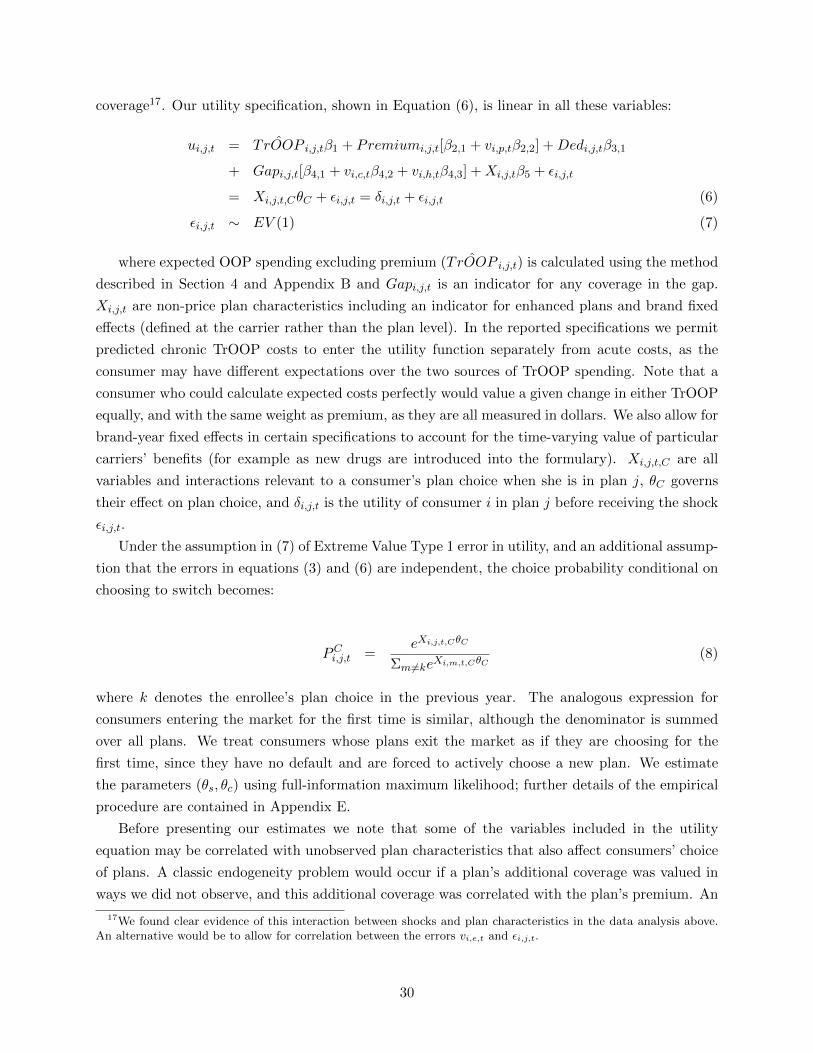
coverage17. Our utility specification, shown in Equation (6), is linear in all these variables:

ui,j,t = ˆTrOOP i,j,tβ1 + Premiumi,j,t[β2,1 + vi,p,tβ2,2] +Dedi,j,tβ3,1

+ Gapi,j,t[β4,1 + vi,c,tβ4,2 + vi,h,tβ4,3] +Xi,j,tβ5 + εi,j,t

= Xi,j,t,CθC + εi,j,t = δi,j,t + εi,j,t (6)

εi,j,t ∼ EV (1) (7)

where expected OOP spending excluding premium ( ˆTrOOP i,j,t) is calculated using the method

described in Section 4 and Appendix B and Gapi,j,t is an indicator for any coverage in the gap.

Xi,j,t are non-price plan characteristics including an indicator for enhanced plans and brand fixed

effects (defined at the carrier rather than the plan level). In the reported specifications we permit

predicted chronic TrOOP costs to enter the utility function separately from acute costs, as the

consumer may have different expectations over the two sources of TrOOP spending. Note that a

consumer who could calculate expected costs perfectly would value a given change in either TrOOP

equally, and with the same weight as premium, as they are all measured in dollars. We also allow for

brand-year fixed effects in certain specifications to account for the time-varying value of particular

carriers’ benefits (for example as new drugs are introduced into the formulary). Xi,j,t,C are all

variables and interactions relevant to a consumer’s plan choice when she is in plan j, θC governs

their effect on plan choice, and δi,j,t is the utility of consumer i in plan j before receiving the shock

εi,j,t.

Under the assumption in (7) of Extreme Value Type 1 error in utility, and an additional assump-

tion that the errors in equations (3) and (6) are independent, the choice probability conditional on

choosing to switch becomes:

PCi,j,t =eXi,j,t,CθC

Σm 6=keXi,m,t,CθC(8)

where k denotes the enrollee’s plan choice in the previous year. The analogous expression for

consumers entering the market for the first time is similar, although the denominator is summed

over all plans. We treat consumers whose plans exit the market as if they are choosing for the

first time, since they have no default and are forced to actively choose a new plan. We estimate

the parameters (θs, θc) using full-information maximum likelihood; further details of the empirical

procedure are contained in Appendix E.

Before presenting our estimates we note that some of the variables included in the utility

equation may be correlated with unobserved plan characteristics that also affect consumers’ choice

of plans. A classic endogeneity problem would occur if a plan’s additional coverage was valued in

ways we did not observe, and this additional coverage was correlated with the plan’s premium. An

17We found clear evidence of this interaction between shocks and plan characteristics in the data analysis above.An alternative would be to allow for correlation between the errors vi,e,t and εi,j,t.

30

insurer with an unobservably good plan who wanted to charge a higher price would submit a higher

bid to CMS, and this would show up as a higher premium. However, the institutional features of the

Part D setting reduce the endogeneity concern considerably. Because plans must meet the CMS’

actuarial standards for coverage for an average statistical person, insurers are not permitted to offer

plans with the types of unobservable quality typical in other differentiated products markets. What

consumers purchase is a tariff; any given treatment does not vary in its characteristics across plans,

and coverage is regulated by CMS; hence the most obvious way to differentiate in an unobservable

dimension is via customer service, which anecdotally does not appear to be a very important force

in this market [29]. Moreover, the persistent presence of overspending even by consumers switching

plans, as well as the lack of dependence on OOP costs shown in our analysis of the data, suggests

that individual firm-specific variation in OOP costs is not driving consumer choices. Hence the

typical unobserved quality dimension correlated with premium, as in Berry (1994) [9], is unlikely

to play a major role in this market. One possible exception is the additional coverage offered

by enhanced plans, which is subject to less tight regulatory scrutiny than that of basic plans.

We include enhanced plan fixed effects in all specifications and add enhanced-year interactions to

account for time variation in the quality of enhanced plan coverage in some specifications.

A second possible endogeneity concern is the fact that we predict consumer out of pocket pay-

ments using observed chronic drug utilization and demographic and utilization types, as described

in Appendix B. If there is some error in this calculation it means we predict an out of pocket cost

for particular consumers that is different from their own prediction. This could mean that some

plans are perceived to be more attractive by particular consumers than is indicated by our OOP

spending variable. Although in the aggregate the predictions of the out-of-pocket payment model

are accurate, if these expectations are mis-estimated in a systematic way for a particular plan, the

error may be correlated with the premium and this could lead to bias in the premium coefficient

(and that on premium shocks). For example, if a plan offers a low-priced version of a chronic drug,

many consumers might choose to switch to it if they enroll in that plan. Our OOP cost measure

assumes that consumers do not switch chronic drugs, so we would predict a higher OOP cost of the

plan than their perception. If premiums are increased to account for this “unobserved generosity”

of the plan, the estimated premium coefficient will be biased towards zero. We include carrier fixed

effects in all specifications to address this issue (since the formulary is usually fixed across plans

within a carrier), and in the final specification we also include carrier-year fixed effects.

6.3 Demand Estimates

The estimated coefficients and standard errors for four separate demand specifications are

shown in Table 13; the means and standard deviations of the variables used in estimation are

reported in Appendix Table A5. Columns 3 and 4 of Table 13 report the estimates from the main

specifications. Model 1 uses brand fixed-effects and an enhanced plan dummy while Model 2 uses

brand-year fixed effects and interacts the enhanced dummy with year fixed effects. Both models

separate TrOOP costs into a chronic and an acute component. The switch parameter estimates

31

indicate that consumers are more likely to switch plans if they receive premium or coverage shocks

or have an acute shock to their health. Women, as well as nonwhite, lower-income and older

enrollees have lower threshold values to trigger awareness, and hence are more likely to switch.

These results are consistent with the probit regression estimates shown in Table 11 and also with

intuition. Overspending mistakes are more costly for older enrollees who spend a higher fraction

of their income on drugs and for lower-income enrollees for whom the excess spending is more

burdensome. For this reason they tend to require smaller prompts in order to re-optimize their

choice.

The third panel of Table 13 sets out the estimated choice coefficients. As noted in the previous

literature, if consumers are risk neutral and perfectly predict their expected OOP costs, we expect

the coefficients on TrOOP and premium to be negative and approximately equal in magnitude and

the coefficients on deductibles and gap coverage to be zero (since their impact on OOP costs is

accounted for in the TrOOP variable). As in AG [2], the estimates do not satisfy these criteria.

Consumers place a much greater negative weight on premiums than on TrOOP18. A one-standard-

deviation (or $241) increase in premium for a single plan, holding all other plans’ characteristics

fixed, generates an average reduction in the probability that the plan is chosen of 24.1%, while

a one-standard-deviation increase in chronic TrOOP, which is a much larger dollar increase of

$935, leads to a 31.4% reduction in probability of choice. Consumers are also estimated to place

significant weights on gap coverage and deductibles. A one-standard-deviation ($126) increase in

deductibles generates a 10.7% reduction in probability the plan is chosen on average, while for plans

offering coverage in the gap, eliminating that coverage results in a 30.2% reduction in the average

probability that the plan is chosen.19 In addition the coefficient on expected acute TrOOP costs is

positive, although small in magnitude relative to the other coefficients.

One possible interpretation of these findings, consistent with the rational inattention framework

discussed above, is that consumers face costs of processing information which prevent them from

accurately predicting their OOP costs in different plans. In that case we should expect the coefficient

on premium - the most readily-observed component of the overall cost - to be larger than that on

chronic TrOOP20. Consumers might also place a significant weight on deductibles and gap coverage

as proxies for expected out-of-pocket costs. Similarly, the counter-intuitive coefficient on acute

TrOOP costs may be partly due to the inherent difficulty in forecasting acute health expenditures;

it might also be capturing the willingness of sicker enrollees to pay more for particular brands.

The choice equation also identifies a second source of frictions in consumer decision-making.

Consistent with the evidence presented in Table 12 as well as that in Busse et al. (2012) [10],

consumers who switch plans following a shock to premiums place additional negative weight on

18Evidence for consumers over-weighting premiums and other plan variables relative to expected costs in otherinsurance markets is presented in Handel (2012) [30] and Ericson and Starc (2013) [22].

19These results imply that eliminating gap coverage is roughly equivalent to a $205 increase in premium, a $355increase in deductible, or a $900 increase in chronic TrOOP.

20It is also possible that our predictions of the TrOOP variables contain measurement error, leading to attenuationbias in their coefficients. This seems more likely for acute than for chronic TrOOP, particularly given the very detailedconsumer-specific data used to calculate the chronic TrOOP variable.

32

Table 13: Estimated Structural Demand Coefficients

No Switch 1 No Switch 2 Model 1 Model 2

Switch ParametersThreshold Shifters Coeff. S.E. Coeff. S.E. Coeff. S.E. Coeff. S.E.

Year (2007) - - - - 4.51*** 0.023 4.37*** 0.023

Year (2008) - - - - 4.62*** 0.023 4.43*** 0.023

Year (2009) - - - - 5.62*** 0.025 5.43*** 0.025

Female - - - - -0.29*** 0.011 -0.22*** 0.011

Nonwhite - - - - -0.07*** 0.018 -0.04** 0.018

Q1 Income - - - - -0.53*** 0.015 -0.47*** 0.015

Q2 Income - - - - -0.32*** 0.015 -0.26*** 0.015

Q3 Income - - - - -0.27*** 0.015 -0.21*** 0.015

Age 70-74 - - - - -0.11*** 0.017 -0.27*** 0.017

Age 75-79 - - - - -0.31*** 0.018 -0.46*** 0.018

Age 80-84 - - - - -0.41*** 0.018 -0.55*** 0.018

Age U-65 - - - - -0.57*** 0.024 -0.83*** 0.023

Age O-85 - - - - -0.62*** 0.017 -0.76*** 0.017

Shocks Coeff. S.E. Coeff. S.E. Coeff. S.E. Coeff. S.E.

Premium Shock - - - - 2.05*** 0.013 1.97*** 0.012

Coverage Shock - - - - 1.75*** 0.014 1.64*** 0.014

Acute Shock - - - - 0.59*** 0.020 0.49*** 0.020

Choice Parameters Coeff. S.E. Coeff. S.E. Coeff. S.E. Coeff. S.E.

TrOOP (Chronic) -1.12*** 0.007 -0.96*** 0.007 -1.14*** 0.010 -0.83*** 0.009

TrOOP (Acute) 0.42*** 0.012 .23*** 0.013 0.61*** 0.013 0.27*** 0.015

Deductible -3.02*** 0.019 -3.87*** 0.045 -2.08*** 0.029 -0.91*** 0.015

Annual Premium -3.36*** 0.014 -4.08*** 0.077 -5.5*** 0.011 -4.36*** 0.026

Premium Shock x Prem - - - - -3.74*** 0.042 -2.66*** 0.039

Coverage Shock x Gap Cov - - - - -0.02 0.017 -0.13*** 0.020

Acute Shock x Gap Cov - - - - 0.63*** 0.028 0.54*** 0.029

Gap Coverage 0.38*** 0.004 0.85*** 0.024 1.00*** 0.010 0.69*** 0.012

Enhanced -0.57*** 0.005 - - -0.25*** 0.007 - -

Enhanced (2006) - - -0.73*** 0.013 - - 0.06*** 0.013

Enhanced (2007) - - -1.05*** 0.012 - - 0.11*** 0.011

Enhanced (2008) - - -0.83*** 0.007 - - -0.48*** 0.012

Enhanced (2009) - - -0.40*** 0.006 - - 0.67*** 0.014

Fixed Effects Brand Brand-Year Brand Brand-Year

N 580,746 580,746 580,746 580,746

Notes: Estimates from two-stage demand model. Threshold Shifters and Shocks are variables that affectthe probability of switching. Choice Parameters are variables that affect preferences for plans conditional onswitching. TrOOP is predicted out-of-pocket cost excluding premium. TrOOP, Deductible and Premium arein $000 per year. Gap Coverage is an indicator for any coverage in the gap. White HCE Standard Errors.“*” = 90% Significance, “**” = 95% Significance, “***” = 99% Significance

33

premiums in making their choice. Likewise consumers place additional positive weight on gap

coverage following a shock to their health status (although not following a shock to their previous

plan’s coverage). The remaining coefficients indicate that brand fixed effects (not reported) are

often large and significant: consumers are willing to pay on the order of $1000 to move from

the second-lowest-value to the second-highest-value plan. Conditional on all other plan variables,

consumers show a slight aversion to enhanced plans on average. When we break out the enhanced

plan coefficient by year in Model 2 the coefficient becomes positive and significant in every year

except 2008.21

We also present, in columns 1 and 2 of Table 13, the results of estimating the choice model

without an initial stage where consumers experience shocks and choose whether to switch. This

specification is very similar to that in AG [2]. Essentially the model estimates the preferences de-

rived from averaging over the behavior of both inattentive and attentive consumers. Consistent with

AG, the estimates indicate that the average consumer under-weights TrOOP relative to premiums,

deductibles and gap coverage; in addition the coefficient on enhanced plans is negative in every

year. Comparing across columns, when we add the first stage switching model the coefficients on

enhanced plans and deductibles become less negative (more “rational” in the sense of risk-neutral

fully-informed consumers choosing the utility-maximizing option), while those on premiums and

gap coverage become slightly larger in magnitude (less “rational”). We explain these changes as

follows. The upwards shift in the enhanced plan coefficients is consistent with inattentive consumers

not noticing that increasingly attractive enhanced plans are being offered over time and therefore

not switching to them; the single-stage model interprets this as a negative utility from enhanced

plans, whereas in the full model we see that this lack of switching is due to inattention. The up-

wards shift in the deductible coefficient is similar. In the single-stage model this coefficient is very

large and negative; it suggests that consumers over-weight deductibles when making choices. When

we add switching to the model we see that this “over-weighting” is partly caused by inattentive

consumers not considering moving into the other (high-deductible) plans available to them22.

These findings suggest that while consumer inattention, and the extra weight placed on pre-

miums and coverage by enrollees experiencing related shocks, explain some of the choice frictions

identified in the previous literature, some other sources of overspending remain. Some are related

to preferences for non-price characteristics (captured, for example, by the brand and enhanced fixed

effects in our model) while others may be due to consumers finding it difficult to predict counter-

factual out-of-pocket costs. In the counterfactual analyses below we explore the implications of

these findings for the cost savings derived from policies that reduce consumer inattention relative

21Some of the effect of enhanced benefits could be subsumed in the estimate for gap coverage, which many enhancedplans provide and which by 2008 and 2009 had all but vanished from basic plans.

22Conversely, the coefficients on premium and gap coverage seem to be over-weighted in the single-stage modeland become more over-weighted when we add switching. That is, averaging over attentive and inattentive consumersgenerates a smaller, rather than a larger coefficient. This is consistent with inattentive consumers not switching outof their plans when their premiums rise or gap coverage falls relative to others in the choice set. The single-stagemodel interprets this as a relatively low (although still over-emphasized) weight on premiums and coverage whereasin fact it is due to inattention regarding other-plan characteristics. When we add the switching stage we see thatswitchers actually over-weight these characteristics more than the single-stage model would suggest.

34

to policies that address the other frictions as well, for example by allowing pharmacists to make

choices for some consumers. Before conducting these analyses, however, we consider the supply

side of the market.

7 The Supply Side of the Part D Market

The estimated model of consumer demand for Part D plans presented above contains substantial

choice frictions, both due to consumer inattention (as described in Farrell and Klemperer (2007)

[23]) and for other reasons. The frictions caused by inattention induce a tradeoff for insurance

providers between (in the words of those authors) “harvesting” and “investing”. “Investing” is

the process of building up market share via low prices in order to increase future profits, while

“harvesting” is the process of reaping those profits by raising prices on an installed base. Ericson

(2012) [20] finds evidence of this dynamic at work in the Part D market. In this section we present

evidence consistent with this model of insurer pricing behavior.

7.1 The New Jersey Part D Market

To analyze the supply-side of the Part D market, we make use of the dataset of Part D plans

generously provided by Francesco Decarolis (Decarolis (2012) [17]) from CMS files on plans, owner-

ship, enrollment, premiums, formularies, and other characteristics. It covers all plans in all regions

of the US (34) for 7 years from 2006-201223. We focus only on the data covering stand alone Part

D PDPs in New Jersey, as these are the plans which serve the consumers modeled in the previous

section.

There were 43 PDP plans active in New Jersey in 2006, the first year of the Part D program;

this is in line with an average of 42.2 plans per region nationwide. The New Jersey market is fairly

concentrated in every year of our data: measured in terms of enrollees, the 4-firm concentration

ratio begins at 0.862 and declines to .617 in 2008 before rising again to .753 in 2012. Herfindahl

indices show the same pattern, declining from 0.259 to 0.154 between 2006 and 2009 before peaking

at .285 in 2011. There was some plan entry in New Jersey in the first several years of the program

but subsequent entry was limited. A total of 19 plans entered in 2007, joining 36 continuing from

2006, and 9 others entered in 2008, but from 2009 to 2012 no more than 3 plans entered in any

year. After 2008 plan attrition reduced the number of active firms in every year from 57 down to

30 by 2012. In the first few years of the program enhanced plans proliferated rapidly, going from

17 of 43 plans with a combined 12% market share in 2006 to 27 of 52 plans with a combined 31%

market share in 2009. This coincided with a near-continuous shift away from Defined Standard

Benefit plans; by 2012, only 3 such plans remained in the market, down from 8 in 2007. These

statistics, presented in Table 14, suggest an oligopolistic market characterized by increasing product

differentiation and increasing concentration.

23See Decarolis (2012) [17] for a detailed description of the data.

35

Table 14: New Jersey Part D Market Summary Statistics

Year Num Enrollmnt CR-4 HHI Entering Enhanced Enhanced DSB DSBPlans Plans Plans Mkt Share Plans Mkt Share

2006 43 281,128 0.862 0.259 43 17 12.27% 6 12.89%

2007 55 298,978 0.780 0.217 19 27 24.32% 8 10.49%

2008 57 304,198 0.617 0.157 9 29 28.62% 7 5.31%

2009 52 317,997 0.637 0.154 1 27 30.63% 5 0.48%

2010 46 329,178 0.660 0.163 2 24 30.43% 5 2.48%

2011 33 333,553 0.751 0.285 1 15 22.46% 4 2.53%

2012 30 343,886 0.753 0.281 3 14 24.00% 3 0.38%

Notes: Summary statistics on New Jersey Part D plans. Source: aggregate CMS data, generously providedby Francesco Decarolis. Total number of plans includes enhanced, Defined Standard Benefit (DSB), andother standard plans not following DSB coverage terms exactly. The latter are not listed separately in thetable.

7.2 Insurer Pricing Strategies

We now consider what effect consumer inattention, coupled with product differentiation and

imperfect competition, has on insurer pricing strategies in the Part D marketplace. One would

expect a profit-maximizing insurer to set its premiums in a way that took advantage of consumer

choice frictions. In this section we note that the patterns in the data are consistent with this

intuition.

Theoretical models of search frictions have fairly clear predictions for prices. Papers such as

Varian (1980) [52] feature search in an environment of a homogeneous product, multiple sellers, and

heterogeneous consumers. In this model, consumers do not engage in sequential search but rather

“become informed” (perhaps by paying a cost) and at that point know all prices. A consumer

who has experienced a shock and decides to re-optimize her plan choice, enters her ZIP code and

medications in the Part D website and then has access to all firms and prices fits this model well.

The equilibrium symmetric outcome of Varian’s model is price dispersion, which we certainly see in

the Part D marketplace. In particular, Defined Standard Benefit plans are so tightly regulated as

to represent a nearly homogeneous product; the only dimensions in which they differ are customer

service and the particular drugs offered within each Key Formulary Type, though they are con-

strained a choice a treatments for each. Nevertheless, Table 15 shows that price dispersion persists

among Defined Standard Benefit plans. Though the difference between the minimum and maxi-

mum premium is falling over time, there is still considerable variation in the cost of this essentially

homogeneous product by 2012.

36

Table 15: Premium Dispersion in New Jersey DSB Plans

Mean, Equal Std. Dev., Equal Mean, Weighted Std. Dev., Weighted Minimum Maximum

2006 $26.33 $11.33 $9.27 $10.52 $4.43 $35.49

2007 $31.28 $12.44 $10.37 $1.86 $10.20 $47.40

2008 $32.51 $17.61 $31.28 $6.19 $19.20 $69.00

2009 $42.88 $18.08 $29.84 $10.46 $26.60 $72.70

2010 $37.66 $4.88 $32.84 $2.21 $32.00 $42.90

2011 $39.73 $5.73 $37.26 $3.17 $34.20 $47.60

2012 $38.37 $4.20 $37.32 $4.48 $34.80 $43.00

Notes: Summary of premium dispersion in NJ Defined Standard Benefit plans. Premiums are in $ perenrollee per month. “Weighted” means weighted by enrollment.

Another important feature of the Part D marketplace is the existence of switching frictions. We

model these frictions as limited attention rather than an explicit switching cost but the effect on

insurer behavior is similar. The classic switching cost model of Klemperer (1987) [40] captures the

main intuition of the firm’s problem. If consumers enter the market in period t and choose among

firms in that period (and by assumption pay no switching costs in the first period), the firm has

an interest in capturing them with a low price (invest). The switching cost the consumer must

pay in order to change plans later causes her to be unwilling to switch in response to small price

differences. Thus the firm can raise price by a small amount in period t + 1 without losing the

consumer (harvest)24. A critical element of this model is that firms cannot discriminate between

new and old consumers; likewise, in Medicare Part D the firm must choose one price for both types

of consumers. 25

Table 16 shows that, consistent with this prediction, premiums increase on average almost every

year. The average annual premium increase for basic plans (weighted by enrollment) is small, less

than $6 per month in every year. Premiums for enhanced plans increase more quickly; in 2008,

the weighted-average premium increase for enhanced plans is over $14 per month, and in 2011 and

2012 smaller enhanced plans post large premium increases. We flag plans that raise premiums by

more than $10. These are tabulated in the second panel of Table 16. Enhanced plans always have

a higher probability of a jump in a given year than basic plans. For three years from 2008 to 2010,

at least a third of enrollees in enhanced plans face large premium shocks, although the rate is lower

in other years.

We can also use the intuition from the theory to predict differences in premium growth across

insurers. First, the change in profit for a given change in price is a function of both the intensive

margin (profit per enrollee) and the extensive margin (number of enrollees). Since larger firms

24The papers on consumer search and learning referenced above (Benabou and Gertner (1993) [7], Fishman (1996)[24], Cabral and Fishman (2012) [13]) also consider how firms price in response to consumer search. They containsimilar intuition and make the point that the equilibrium outcome for prices depends on the size of the search costrelative to the variation in firm costs of production.

25Since firms can sponsor more than one plan, we might expect to see segmentation of consumers and pricediscrimination as in Ericson (2012) [20]. In our supply-side model we simplify by abstracting away from multi-product strategies and concentrate on the invest versus harvest tradeoff.

37

Table 16: Average Premium Increase and % of Plans with $10 Premium Increase

Premium Increase ≥ $10 Premium Increase

Equal Equal Weighted Weighted Equal Equal Weighted WeightedBasic Enhanced Basic Enhanced Basic Enhanced Basic Enhanced

2007 -$2.94 $1.01 -$2.20 $7.20 33.33% 40.74% 0.33% 10.53%

2008 $4.65 $11.50 $5.93 $14.45 39.29% 55.17% 24.10% 39.82%

2009 $6.20 $7.12 $3.68 $4.39 24.00% 33.33% 0.83% 39.31%

2010 $5.06 $1.77 $2.92 $5.44 21.74% 29.17% 1.19% 35.08%

2011 $1.04 $14.33 -$3.09 $2.84 11.11% 73.33% 6.50% 24.48%

2012 -$1.24 $6.52 $1.97 $2.02 12.50% 42.86% 0.16% 16.38%

Notes: Summary of premium changes ($ per enrollee per month) over time for New Jersey PDPs, by Yearand Plan Type

have a larger intensive margin, we should expect large firms to raise prices more than smaller firms

all else equal. Second, we should expect slower premium growth when the number of consumers

purchasing for the first time is high relative to the size of the installed base. Thus premiums should

rise more slowly in years with high attrition (e.g. high death rates) or large cohorts aging into

the Part D program. Because of our focus on shocks to consumers’ attention and the dynamics

of pricing, we do not estimate our motivating regression in levels like Polyakova (2013) [44], but

rather in premium changes. It is the increase in price that becomes more lucrative with an increase

in installed base. We therefore estimate regressions of annual premium increases on lagged market

shares, growth rates, and other plan variables that might affect costs for all PDP plans in the

national dataset.

Table A4 in the Appendix reports the coefficients. When we control for region and carrier

fixed effects and coverage variables that may affect costs, lagged market shares significantly predict

future increases in premiums, providing evidence in support of the first hypothesis. The estimates

also indicate that the growth rate of enrollment in the region, which we treat as a proxy for new

enrollment, is negatively associated with price increases. This result provides evidence for the third

hypothesis, that price competition is more aggressive (with smaller price increases) when there

are relatively more unattached consumers to compete for. Taken together, the results of these

models provide suggestive evidence in favor of firms pursuing pricing strategies similar to those in

Klemperer (1987) [40] and Farrell and Klemperer (2007) [23].26

26The observed pattern of price increases could potentially be due to unobserved quality; plans with higher qualityare more attractive to enrollees, leading to higher market shares, and are also able to raise prices as a result. Forseveral reasons this is unlikely to account for the observed price increases. First, the model controls for brand fixed-effects, and thus accounts for any unmodeled dimension of quality which is fixed at the carrier-level (and as discussedwe believe this covers most such dimensions). Second, the coefficient on lagged market share is still positive evenwhen we restrict the sample to Defined Standard Benefit plans (although due to lack of power the coefficient is notsignificant). As mentioned before these DSB plans represent an essentially homogeneous product, suggesting that theharvesting dynamic is active even among non-differentiated plans. Third, individual plans switch between “investing”’and “harvesting” over time in ways that are inconsistent with time-invariant unobserved heterogeneity. For examplethe SilverScript/CVS Caremark enhanced plan reduced premiums by $19 from 2006-7 and by $8 between 2007-8,resulting in substantial increases in market share. Over the next four years the plan’s premium growth was well abovethe market growth rate. Over the same time period the Humana enhanced plan pursued the reverse strategy, raising

38

7.3 Insurer Cost Estimates

Our next step is to use accounting data to estimate each plan’s average cost per enrollee. These

costs will be used as an input to the counterfactual premium simulations in the following section.

We have applied for plan-level cost data from CMS. For now we use our claims data for New Jersey

to approximate the required cost information.

The claims data indicate the gross drug cost for every claim, including the drug ingredient cost

plus the dispensing fee and sales tax paid to the pharmacy, but not accounting for manufacturer

rebates or plan administrative costs. For each branded drug we find the average gross drug cost of a

thirty-day supply across all plans and all encounters in the relevant year and apply a 20% rebate to

that average cost. For generic drugs we assume a $4 cost per 30 day supply for all plans27. We use

these figures, and the observed drug utilization for each enrollee, to predict an average drug cost

net of rebates per enrollee per year. Our methodology also accounts for the fact that, as part of

its risk-adjustment strategy, the government covers 80% of all drug costs in the catastrophic phase

so that the plan pays at most 20% of these costs.28 We inflate the resulting cost per enrollee per

year by 116% to account for administrative costs29. Finally we winsorize the data at the 5 percent

level within each plan and year to remove outliers before constructing an average plan-level cost

per enrollee per year. 30

The predicted plan costs per enrollee generated using this method are summarized in Table

17. We report weighted averages and medians of both the estimated total cost per enrollee and

the estimated cost net of enrollee out-of-pocket payments31. The latter will be the cost variable

used as an input into the premium-setting simulations below. Finally we report for comparison

the weighted average observed bid and observed premium separately for each year of our data.

Observed bids are slightly higher than predicted costs net of TrOOP on average in 2006, the first

year of the program. Observed bids fall on average in the second year, and this together with

premiums by $23 and $26 in 2007 and 2008 and then switching to below-market price increases in 2009. We interpretthese patterns as evidence that particular plans switch from being “investors” to “harvesters” over time in responseto changes in market share. Another potential alternative explanation for the patterns observed in the data is thatpremiums are mean-reverting; the firm prices low in one year, attracting a large market share, and upon realizing aloss increases prices in the next year, leading to the observed correlation. However, this does not explain why somefirms maintain large market shares even after increasing premiums quite steeply. Moreover, this strategy would notbe profit-maximizing unless choice frictions of the type described above were present.

27A study by the Department of Health and Human Services Inspector General (Levinson (2011) [42]) found that, in2009, rebates reduced Part D drug expenditures by 19% on average for the 100 highest-volume brand name drugs. Weassume a slightly lower percentage to account for potentially lower rebates for lower-volume drugs. Our assumptionregarding generic drug costs is based on Walmart’s well known “$4 for any generic prescription” program.

28In most cases the beneficary pays a 5% copay as well, so for branded drug events in the catastrophic phase weassume the plan pays 15%. Fewer than 5% of enrollees ever reach the catastrophic phase so this has little effect onpredicted plan costs.

29Sullivan (2013) [51] notes that the National Health Expenditure Accounts (NHEA) includes the administrativecosts of Medicare Advantage plans and Part D plans in its report of total Medicare administrative costs. We usethis fact, and data from the NHEA for 2006-2010, to back out administrative expenses of 14-16% of total costs - or16-19% of non-administrative costs - for Parts C and D combined.

30Additional details of how these cost numbers are constructed are contained in Appendix F.31We truncate the plan-level average cost net of OOP payments at zero; this step involves only a few plans.

39

an increase in estimated costs implies a lower average markup32. Bids increase much faster than

predicted costs in the following two years. While these predictions are likely to change when we

obtain access to more detailed cost data from CMS, the estimates shown here clearly indicate that

plan margins did not converge towards zero over the first few years of the program.

Table 17: Bids and Estimated Plan Costs for New Jersey PDP Plans

Observed Bid Observed Premium Predicted Cost Pred. Cost net of TrOOP

W. Ave (SD) Median W. Ave (SD) Median W. Ave (SD) Median W. Ave (SD) Median

2006 $63.03 ($28.50) $69.48 $24.00 ($10.23) $24.24 $135.19 ($35.97) $131.69 $62.15 ($23.18) $55.41

2007 $60.44 ($24.43) $74.70 $25.05 ($11.92) $25.40 $150.98 ($34.37) $145.39 $69.31 ($16.21) $63.72

2008 $87.25 ($25.70) $93.41 $35.29 ($15.83) $32.40 $142.64 ($39.53) $130.72 $71.52 ($31.19) $58.51

2009 $94.73 ($26.91) $102.50 $40.34 ($15.22) $36.90 $144.20 ($37.63) $136.72 $74.36 ($38.48) $57.14

Notes: Summary of weighted average and median observed bids, observed premiums, predicted costs to theplan, and predicted costs net of enrollee out-of-pocket payments. All figures are per enrollee per month.Weighted standard deviations in parentheses; weighted by enrollment.

8 Counterfactual Simulations

Medicare Part D is difficult for consumers to navigate, and as already noted, previous studies

have considered the effects of various interventions designed to ease the decision-making process.

For example, in a randomized experiment, Kling et al. (2012) [41] provide information to Part D

enrollees regarding their best plan choice, and find that it increases the probability of switching by

11 percentage points. 33Abaluck and Gruber (2013) [1] predict that if an intervention could make

consumers fully informed and fully rational, they would choose plans that reduced their costs by

about 27%. However these papers do not estimate sufficiently detailed models of consumer demand

to permit simulations of the impact of policy experiments that “switch off” particular components

of consumer choice frictions. Perhaps more importantly, they do not account for the issue that plans

are likely to change their pricing strategies in response to changes in consumer behavior, potentially

further lowering program costs. In this section we will address both issues. Our demand model

allows us to remove each of the different sources of consumer choice error in turn. We then use the

firm cost data set out in the previous section, together with a model of firm behavior, to consider

price changes in response to the changes in consumer choices. That is, we estimate the impact of

reducing consumer inattention on overall program costs, taking into account plans’ price responses

to this change.

32The markup is not exactly the bid less the cost and for this reason we do not report a markup estimate based onthese data. Plan revenues also include an additional premium amount for enhanced plans plus reinsurance paymentsfrom CMS. See the plan profit equation in Section 8 for details.

33While the rather modest efficacy of this experiment may in part be explained by the relatively low dollar amountsat stake in Medicare Part D and the reduced cognitive capacity of older beneficiaries, Cronqvist and Thaler (2004) [15]document similar experiences with an advertising campaign intended to deter people from selecting the default optionfollowing a redesign of the Swedish pension system. The confirmation of these results among younger participantswith greater stakes suggest that they are not a feature unique to Medicare Part D.

40

8.1 Simulations Holding Prices Fixed

Our choice model identifies several sources of frictions: inattention, which prevents switching

until the consumer experiences a shock to her health or her own plan’s price or coverage; the

impact of shocks on preferences when choosing a new plan; and the fact that switchers place a

larger weight on characteristics like premium and gap coverage than would be the case for risk-

neutral fully-informed consumers choosing the plan with the lowest expected costs. We now predict

the effects of different counterfactual policies that address some or all of these frictions under the

assumption that all lead to errors that the social planner would wish to correct.

We begin by simulating the effect of replacing the existing default (that each consumer remains

in her current plan unless she chooses to switch) with the default that she exits the program. In

our model this has the effect of removing consumer inattention.34 Actual choices will still be made

with the estimated preferences from Table 13 except that we suppress the effect of past shocks on

preferences in this simulation. When all consumers re-optimize each year, shocks will no longer

affect preferences35. In order to compare simulated-to-simulated choices, we also estimate choices

under the full frictional model specified in Section 6.2 and treat these estimates as the “baseline”.36

Our third counterfactual policy addresses the issue that even attentive consumers do not make

cost-minimizing choices. We simulate the impact of a policy that pays the pharmacist $50 each

time he moves an enrollee to one of her five lowest expected-cost plans, if moving would save her

at least $200 on average. We consider this policy for two reasons. First it removes all sources

of consumer overspending rather than just inattention. By involving a pharmacist in the choice

process, who is assumed to use the online CMS plan finder tool, we remove all choice frictions

and unambiguously place the enrollee in one of the lowest expected-cost plans (although we note

that, due to acute shocks, it may not turn out to be the cheapest plan in the current year).37

We further assume that the pharmacist has the same expectations as the enrollee over chronic

and acute prescriptions, is independent of all insurers, and cannot be compensated or incentivized

by an insurer. This policy simulation also avoids a potential problem that was assumed away in

the first counterfactual: some consumers might respond to the “no default” policy by exiting the

program. We assume that enrollees who are moved by their pharmacist do not switch away from

the pharmacist’s chosen plan. Other enrollees, whose choices the previous year were within $200

of the optimal choice, continue to make choices based on our two-stage demand model.

Finally we conduct a slightly different pharmacist-based simulation. Here we address an is-

sue with the previous counterfactual: the allocations made by the pharmacist in that simulation

34The evidence in Heiss et al. (2006) [34] suggests that few consumers would choose to exit the program ratherthan re-optimizing. There is also a considerable literature on the importance of default choices in the context of otherbenefits such as retirement savings.

35 This is consistent with a model where the increased importance of a characteristic such as premium following ashock is due to its relevance in prompting the consumer to re-optimize. However we note that the results are similarif shocks are allowed to interact with preferences.

36Details of how these choices are simulated are provided in Appendix F.37It is also possible that the pharmacist’s choice would be constrained by the pharmacy network offered by each

plan. For now we abstract away from this issue.

41

overrode consumer choices that were partly due to preferences for non-price characteristics (e.g.

the brand and enhanced fixed effects in our model) which may have led to overspending by our

definition but did not correspond to choice mistakes. To address this we consider an analogous

policy, except that now the pharmacist is paid $50 for moving enrollees to another plan within the

same brand if this would save over $200 in expectation. This simulation removes overspending due

to consumer choice frictions while respecting their preferences for particular insurance carriers.

8.2 Allowing Insurers to Change Prices

The second set of counterfactuals uses our plan cost data as an input to a simulation of supply

side changes in response to changes in consumer choice. We focus on the simple counterfactual

where consumer inattention is removed and preferences are not affected by shocks experienced in

the previous year. We note that while the firm pricing problem in the observed data is dynamic,

the dynamics come only from consumer inattention, i.e. the fact that consumers are “sticky” so

a plan’s price in one period affects its enrollment in future periods. Removing inattention makes

the price-setting process static rather than dynamic, implying that the new equilibrium prices can

be predicted (as a function of costs) using a simple system of static first-order conditions. Since

capturing demand today to “harvest” tomorrow is no longer important in the static problem, we

expect the path of prices to be flatter in our simulations than in the data.

It is important at this point to fix ideas concerning the pricing freedom Part D insurers have.

Recall that each insurer submits a bid for each plan. That bid determines the price in the mar-

ketplace (by the amount over the base beneficiary premium). Importantly, each basic plan must

offer actuarially equivalent coverage if it does not follow the tariff set out in the law. This means

that for a CMS-defined statistical person, the mean of out of pocket charges must be the same in

expectation for all basic plans, so plans cannot respond to increased consumer premium sensitivity

by reducing premiums while increasing average out of pocket charges. Additionally, the subsidy

for each enrollee is risk adjusted depending on age and chronic conditions. CMS’ risk adjustment

is fairly simple (and therefore surely plans will be able to learn over time, for example, which

diabetics are profitable and which are not). However, risk-adjusted subsidies mean the rewards

to cream-skimming are likely second order. This allows us to abstract from selection issues as we

model the behavior of insurers. We model insurers’ choices of bids while holding the schedule of

out-of-pocket charges fixed.

We write plan j’s profit in year t as:

πj,t = (Bj,t + Ej,t − Cj,t)Nj,t (9)

where Bj,t is the bid made to CMS reflecting the plan’s average monthly revenue requirement

per enrollee in a basic or standard plan including profit, Ej,t is the additonal amount charged to

enrollees in an enhanced plan (the “enhanced premium” discussed further below; this is zero when

42

j is a basic plan), Cj,t is the plan’s cost per enrollee net of enrollee out-of-pocket payments and

Nj,t is its number of enrollees.

The premium charged to enrollees in a standard or basic plan is the difference between the bid

and the proportion of the “national average monthly bid amount” (NAMBA) that is subsidized by

the government:

PremiumBasici,j,t = Bj,t − γtNAMBAt = (1− γt

Jt)Bj,t +

γtJt

Σk 6=jBk,t (10)

where γt is the proportion of the NAMBA that is paid by the government and Jt is the number of

Part D plans included in the average in year t. This expression reflects the fact that, in the first

two years of the program, the NAMBA was an unweighted national average of bids for all MA and

PDP plans. From 2008 on, CMS phased in the implementation of a weighted average, where the

weight was the plan’s enrollment.

The premium charged to enhanced plan enrollees is the basic premium defined in equation

(10) plus the enhanced premium Ej,t. The enhanced premium is negotiated between the carrier

and CMS and is meant to comprise the average additional cost of enhanced benefits provided to

enrollees in the plan. It is not subsidized by CMS. We observe this variable in the data for every

plan-year and account for it in our simulations under the assumption that it does not change in

response to simulated changes in enrollee behavior.

We take several steps to account for CMS’s risk adjustment strategy. The government subsidy,

which is written into law at 74.5% of the NAMBA, is split between a premium subsidy and reinsur-

ance or risk adjustment payments. The latter include a commitment to pay 80% of the total cost

of drugs above each enrollee’s catastrophic threshold and payments to keep plans within symmetric

risk corridors that limit their overall losses and profits. We adjust our measure of plan costs per

enrollee to take account of the catastrophic drug subsidies as described in the previous section.

We use the true proportion of the NAMBA that is paid by the government in every year (which

is observed in our data, e.g. 66% in 2006) as an input to the premium calculation in equation

(10); we then assume that the remaining risk adjustment payments neutralize the effect of enrollee

selection on plan costs so that the cost per enrollee does not change with enrollees’ plan choices in

our simulations.

We implement the “no frictions” assumption by considering a single-stage consumer demand

system. We use the estimated parameters of the choice equation in the third column of Table 13

but set the coefficients on premium, coverage and acute health shocks to zero; this is equivalent

to assuming that every consumer considers switching in every year and that preferences over plan

characteristics are unaffected by shocks38. The resulting utility equation can be written as:

ui,j,t = λi,j,t + β2,1Premiumj,t + εi,j,t = δi,j,t + εi,j,t (11)

38As noted in the previous section the latter assumption has very little effect on the simulations.

43

where Premiumj,t includes the enhanced component of premium where relevant and λi,j,t includes

all consumer and plan-specific variables in the estimated utility equation except the premium.

This utility equation can be used to predict plan enrollment Nj,t under any distribution of plan

characteristics:

Nj,t =

Nt∑i=1

eδi,j,t∑Jtk=1 e

δi,k,t=

Nt∑i=1

Λi,j,t(λi,j,t, λi,−j,t, P remiumj,t, P remium−j,t). (12)

Here Λi,j,t(.) is the predicted probability that consumer i chooses plan j in period t; it is a

function of all plan characteristics including their premiums. We consider plans’ optimal choices in

the static bid-setting game that results from removing consumer choice frictions. The first-order

condition for plan profits with respect to the bid Bj,t is:

(Bj,t + Ej,t − Cj,t)∂Nj,t

∂Bj,t+Nj,t = 0. (13)

Calculating the derivative∂Nj,t

∂Bj,trequires us to predict the effect of a change in the bid Bj,t on

the premium. We use the expression in equation (10) under the assumption that the NAMBA is

an (unweighted) average for PDP plans in New Jersey and that plans internalize their impact on

the NAMBA, and therefore on the government subsidy, when choosing their bids39. We predict

the resulting effect on enrollment using equation (12). The first order condition simplifies to the

following expression:

Nt∑i=1

Λi,j,t(.) + (Bj,t + Ej,t − Cj,t)Nt∑i=1

(β2,1Λi,j,t(.)(1− Λi,j,t(.))) = 0 (14)

where we omit the arguments of Λi,j,t(.) for ease of exposition. All plans’ bids enter this equation

through Λi,j,t(.) as well as through Bj,t. We solve this system of equations to obtain the implied

new equilibrium for bids40.41

8.3 Simulation Results

The simulation results are set out in Tables 18A, 18B, 19 and 20. Table 18 considers the impact

of altering consumer behavior without allowing premiums to change in response. The column

labeled “baseline” in Table 18A shows the cross-enrollee average of annual premium costs and

39We account for the fact that a change in one plan’s bid will affect all plans’ premiums via the subsidy.40In reality the NAMBA is a national average, and includes MA as well as PDP plans, so our use of a NJ average

for PDP plans is a simplification. In reality plans have less impact on the NAMBA than they do in our simulations.However in our model this will not affect the equilibrium bids since the impact of the bid on the NAMBA andtherefore the subsidy leads to the same change in the premiums of all plans. In a logit specification this has no effecton product market shares so changing the extent to which a single plan can affect the NAMBA will not change theoptimal predicted bids.

41Additional details of this derivation are provided in Appendix F.

44

out-of-pocket costs (including premiums) predicted by our demand model including all frictions42

The second column (“Lowest Predicted Cost”) shows the same simulated costs when every enrollee

chooses the plan with the lowest predicted costs to her in the relevant year; this is the lowest-cost

outcome possible. Column 3 shows the average simulated costs from the five lowest predicted-cost

choices for each enrollee. We view this as a more realistic “best case” scenario since choosing the

lowest-cost plan may conflict with consumer preferences regarding brand visibility or other non-

price issues. Column 4 of Table 18A shows costs simulated using the “no frictions” model with

both inattention and the effect of shocks on preferences removed. In each column, the row labeled

“Total” provides cumulative spending per enrollee over the four years we consider. “Saving” is

the difference between that cumulative spending and the spending in the baseline scenario, and

“% Fixed” is the proportion of the saving from moving every consumer to the average of her five

lowest-cost plans that is achieved by the relevant counterfactual.

In the first year of the program the choices in the “no frictions” counterfactual are the same as

the baseline (since there can be no inattention; all consumers are entering the program). Even in

that year, however, savings of approximately $432 per person would be generated if enrollees could

be switched to their lowest-cost plan. Cumulative savings over the four year period from moving

everyone to the lowest-cost plan would be approximately $1,753 per person, or 34.7% of the total

baseline out-of-pocket cost. The total saving from moving each enrollee to the average of her five

lowest-cost plans is $1,289 or 25.5% of the total baseline cost. The savings from removing choice

frictions begin in 2007 with a total saving of approximately $14 per person and rise to $70 per person

in 2008 and $62 per person in 2009. Overall the model predicts that the average consumer saves

$145 cumulatively across the four years when frictions are removed, or 11.3% of total overspending.

While these savings are non-trivial, they do represent a fairly small proportion of total overspending.

This is unsurprising given the frictions that remain in the utility equation used to simulate choices.

We should not expect our simulations to bring overspending below the level reached by observed

switchers in the data; that level, defined as a percent of total spending, is approximately 26-28%

(Table 6A) and our simulations generate errors of a very similar magnitude. We also note that,

since our demand estimates indicate consumers respond more strongly to premiums than to TrOOP,

removing frictions should primarily save money through consumers choosing low-premium plans.

Consistent with this intuition, 63% of the savings from removing choice frictions come from lower

premiums. Savings are concentrated in 2008 and 2009 when the baseline choices are most affected

by inattention.

42The difference between “baseline” and “lowest-cost” in Table 18A is slightly different from the panel labeled “FullSample” in Table 5 because the baseline in Table 18 uses predicted choices from our demand model rather than thechoices observed in the data.

45

Table 18A: Simulated Per-Person Spending Holding Premiums Fixed

Baseline Lowest Pred. Cost Lowest 5 Average No Frictions

Premium OOP Premium OOP Premium OOP Premium OOP

2006 $300.98 $1,222.00 $124.54 $790.20 $214.20 $948.40 $300.98 $1,222.00

2007 $322.74 $1,228.40 $232.74 $857.32 $270.22 $949.72 $321.51 $1,214.80

2008 $461.88 $1,265.20 $261.53 $820.94 $282.30 $900.24 $405.40 $1,195.50

2009 $503.98 $1,325.60 $290.19 $819.75 $338.94 $954.02 $469.59 $1,263.80

Total $1,589.58 $5,041.20 $909.00 $3,288.22 $1,105.65 $3,752.38 $1,497.39 $4,896.10

Saving - $0 - $1,752.98 - $1,288.82 - $145.10

% Fixed - 0% - - - 100% - 11.26%

Notes: Results of counterfactual simulations holding premiums fixed at observed levels. Simulated out-of-pocket costs are cross-enrollee averages per enrollee per year including premiums. Premiums include bothbasic and enhanced premium.

Table 18B: Simulated Per-Person Spending, Premiums Fixed, Pharmacist Simulations

Baseline Lowest 5 Average Pharma (Low-5 Avg.) Pharma w/in-Brand

Premium OOP Premium OOP Premium OOP Premium OOP

2006 $300.98 $1,222.00 $214.20 $948.40 $224.17 $990.94 $279.09 $1,126.41

2007 $322.74 $1,228.40 $270.22 $949.72 $271.00 $1,010.04 $284.50 $1,112.49

2008 $461.88 $1,265.20 $282.30 $900.24 $314.24 $968.95 $383.56 $1,125.56

2009 $503.98 $1,325.60 $338.94 $954.02 $368.05 $1,021.18 $440.69 $1,193.26

Total $1,589.58 $5,041.20 $1,105.65 $3,752.38 $1,177.46 $3,991.12 $1,387.84 $4,557.72

Saving - $0 - $1,288.82 - $1,050.08 - $483.48

% Fixed - 0% - 100% - 81.48% - 37.51%

Notes: Results of counterfactual simulations holding premiums fixed at observed levels. “Pharma” is phar-macist. Simulated out-of-pocket costs are cross-enrollee averages per enrollee per year including premiums.Premiums include both basic and enhanced premium.

Table 18B repeats the baseline and five-lowest-cost estimates for comparison and shows the

simulated outcomes in the policy experiments where pharmacists are involved in plan choice. The

out-of-pocket costs include the $50 payment to the pharmacist per switched enrollee. In column 3

the pharmacist can move the enrollee to any plan43; in column 4 she can be moved only to other

plans within the same carrier. The “no frictions” counterfactual demonstrated that approximately

11% of overspending in our setting was due to consumer inattention. The “pharmacist” counter-

factuals address the remaining 89% which is attributable to other factors such as enrollees placing

a high weight on particular characteristics (e.g. brand, premium or gap coverage) rather than min-

imizing overall costs. As shown in Columns 3 and 4 of Table 18B, pharmacists are very effective in

reducing costs. Even though the payments made to pharmacists are included in the OOP costs, the

first pharmacist counterfactual generates savings of $1,050 per enrollee over the four year period,

43We use the average of the five lowest-cost plans for each enrollee. The savings from moving enrollees to the singlelowest cost plan are approximately four percentage points higher.

46

or 81.5% of the total baseline error. Approximately 65% of enrollees are switched to low-cost plans

by the pharmacist, and since those making the largest errors are the ones targeted, the cost of the

pharmacist payments are small relative to the savings. While we stress that not all the frictions

removed here are necessarily due to consumer errors - they may represent heterogeneous preferences

that the social planner would not wish to ignore - the magnitudes of the cost savings from this

counterfactual are considerable. We also note that, when the pharmacist is restricted to moving

enrollees to other same-carrier plans, the savings fall to 37.5% of the total baseline error. While

consumers may have preferences for particular brands, and this may be one reason why they do

not choose the lowest-cost plan available, the benefit to the enrollee from staying within-brand may

not be as great as the cost.

Tables 19 and 20 report the results of the “no frictions” simulations when we allow prices to

adjust. Consider first the cross-plan unweighted average bids reported in columns 1 and 2 of Table

2044. Recall that theory predicts plans should respond to the removal of consumer inattention

(i.e., increased search) by reducing the rate at which they increase prices from year to year. The

observed and simulated bids reported in Table 20 for 2007-2009 are consistent with this intuition.

The average simulated bid in 2007 is very similar to the average observed in the data for NJ

PDP plans (the averages are $77 and $78 per enrollee per month respectively) but simulated bids

increase very little in 2008 and 2009, approximately in line with the rate of cost increases (Table

17), while the observed version has a much higher growth rate. The data for 2006 look different:

while simulated bids are similar to those in other years, observed bids are somewhat higher (at $84

per month compared to a simulated average of $68). Plans may have been experimenting, with

limited information about their competitors’ pricing strategies, in the first year of the program.

Table 19: Simulated Per-Person Spending With Premium Adjustments

Baseline Lowest 5 Ave. No Frictions No Frictions

(Fixed Premium) (Fixed Premium) (Fixed Premium) Premium Change

Premium OOP Premium OOP Premium OOP Premium OOP

2006 $300.98 $1,222.00 $214.20 $948.40 $300.98 $1,222.00 $222.48 $1,166.60

2007 $322.74 $1,228.40 $270.22 $949.72 $321.51 $1,214.80 $178.54 $1,059.00

2008 $461.88 $1,265.20 $282.30 $900.24 $405.40 $1,195.50 $228.00 $1,053.00

2009 $503.98 $1,325.60 $338.94 $954.02 $469.59 $1,263.80 $211.41 $1,038.80

Total $1,589.58 $5,041.20 $1,105.66 $3,752.38 $1,497.39 $4,896.10 $840.43 $4,317.40

Saving - $0 - $1,288.82 - $145.10 - $723.80

% Fixed - 0% - 100% - 11.26% - 56.16%

Notes: Results of counterfactual simulations allowing premiums to adjust to changes in consumer behavior.Simulated out-of-pocket costs are cross-enrollee averages per enrollee per year including premiums. Premiumsinclude both basic and enhanced premium.

Table 19 translates the bids into average per-enrollee premium and out-of-pocket spending

44Table 20 provides averages at the plan level while Tables 18 and 19 contain per-enrollee averages.

47

Table 20: Counterfactual Government Savings

Year Unw. Ave Unw. Ave γt Annual Ave Non-LIS Savings Benefit Costs SavingsObserved Bid Simulated Bid Savings ($) Enrollment ($ billion) ($ billion) (%)

2006 $84.14 $67.76 0.65 $127.95 7,371,512 $0.94 $47.1 2.00%

2007 $78.39 $77.34 0.66 $8.32 8,120,524 $0.07 $48.8 0.14%

2008 $91.49 $81.45 0.65 $78.67 8,413,202 $0.66 $49 1.35%

2009 $107.08 $85.36 0.64 $166.77 8,572,910 $1.43 $60.5 2.36%

Total $361.09 $311.91 - $381.71 32,478,148 $3.10 $205.4 1.51%

Notes: Results of Program Cost Savings Calculation. Columns 1 and 2 are unweighted average bids, observedand simulated, for PDP plans in NJ, measured in $ per enrollee per month. Annual average savings are thedifference between the two average bids scaled by the proportion paid by the government and annualized.Non-LIS enrollment reported in national plan data generously provided by Francesco Decarolis. γt is definedin Section 7.

figures analogous to those in Table 18. The first three columns are repeated from Table 18 for ease

of comparison: these are the baseline, the average of the five lowest-cost plans and the no frictions

scenarios, all holding prices fixed. Column 4 reports the results when we allow plans to re-optimize

prices. Simulated premiums are much lower than the fixed price level in 2006, in line with the

difference between observed and simulated bids. Simulated premiums remain low in later years

while average premium spending derived from observed prices rises every year, again consistent

with average bids45.

These results indicate a large supply side response to the simulated changes in consumer behav-

ior. While removing choice frictions (inattention and the impact of shocks on preferences) resulted

in only small reductions in costs, once premiums are allowed to adjust the savings are substantial.

Plans respond to the newly attentive, premium-sensitive enrollee market by reducing their premi-

ums. The results in the fourth column of Table 19 indicate a saving of $724 per enrollee over four

years or 56% of the total overspending (relative to the 5 lowest-cost plans). Premium reductions

account for essentially all of the estimated savings. Fully 70% of the savings are realized in 2008

and 2009, the years when premiums are particularly high in the baseline data.

Extrapolating these estimates from New Jersey to the entire nation implies substantial govern-

ment savings for enrolled consumers over four years. Program cost savings result mostly from the

slower growth in plan bids, of which the government pays a sizeable proportion. As shown in Table

20, bids in the counterfactual grow at just 5.1% per annum average between 2007 and 2009, relative

to 16.9% in the baseline, and by 2009 the average bid is roughly $260 lower per year in the coun-

terfactual than in the baseline. Applying a conservative assumption that reinsurance costs remain

fixed and the government saves a fraction of the difference in average bids equal to one minus the

Base Beneficiary Percentage (γt in Section 8.2), we find that government savings per covered life

come to $382 over four years. Assuming further that low-income subsidy payments are unaffected

45The premiums in Table 19 are lower than would be implied by the bids in Table 20 because of endogenousenrollment choices. That is, the Table 19 premium numbers are averages across enrollees rather than plans andconsumers tend to choose lower-premium plans, particularly when inattention has been removed. The simulatedpremium numbers are particularly low in 2007-2009 because the cross-plan variation in simulated premiums is high,allowing enrollees more leeway to choose low-premium options.

48

and multiplying this figure by the non-LIS population in each year generates cumulative four-year

savings of $3.1 billion. As with consumer savings, most of the savings are realized from bending

the cost curve downward, and 67% of the savings on program costs are realized in 2008 and 2009,

amounting to 1.9% of total program costs in those years. Combined with the theoretical results

discussed in Section 7 and the results from Table 16, these estimates suggest that program cost

savings from reduced choice frictions are greater in the “harvest” phase than in the “investment”

phase, and it would be reasonable to expect savings in future years to more closely resemble 2008

and 2009 than 2006 and 2007.

We also consider the impact of these policy experiments on plan revenues and margins. Our

estimates indicate that average margins rise in the observed data from approximately $29 per

enrollee per month, or 25% of revenues, in 2006 to $60 or 51% of revenues in 200946. In the

simulations these values fall to stable levels of approximately $18 per enrollee per month, or 28% of

revenues, in every year. In an unregulated market, plans would be likely to respond to these changes

by reducing quality (e.g. the number of drugs included in the formulary) or increasing consumers’

out-of-pocket payments. In Medicare Part D, however, the regulatory requirements described

above restrict plans’ ability to respond in this way, and for this reason (as well as computational

tractability) our simulations hold out-of-pocket costs and formularies fixed. We note that enhanced

plans, whose additional benefits are less tightly regulated, might increase in cost or reduce their

quality in response to the policies we simulate. Even given this caveat, however, the savings from

the above policies are likely to be substantial.

9 Conclusions

In this paper we have developed a model of consumer choice in the Part D program and have

analyzed how firms set prices in response to the presence or absence of those behaviors. We find

that the data support a model where consumers face costs of processing information. This leads

them to avoid making new choices, rolling over their plan selections from one year to the next

unless shocked by a change to their current plan or their current health. When making choices

they also seem to face cognitive costs, under-weighting predicted out-of-pocket payments relative

to plan characteristics that are easier to observe such as premiums and gap coverage.

We provide evidence that firms’ premium choices are responsive to consumers’ search frictions.

In particular, when consumers choose better, firms are incentivized to lower their margins which

results in lower premiums. Using our estimates of consumer behavior and a model of firm price-

setting we simulate the cost effects of different counterfactual policies that could be used to address

these issues. The benefit of removing inattention at fixed prices is fairly small, perhaps because

consumers continue to face cognitive costs when making their new plan choice. However, when

we simulate plans’ premium choices, we predict a large price response to this change in enrollee

behavior. Our simulations indicate that the combination of the demand- and supply-side changes

46The margin is defined as the sum of the bid and enhanced premium less costs net of out-of-pocket payments.

49

would reduce the current overspending relative to consumers’ five lowest-cost options by 56%, even

without addressing enrollees’ other choice frictions. The natural plan response of increasing other

components of the price, like the out-of-pocket cost schedule, or reducing coverage is constrained

by the tightly regulated standard benefit levels. We also consider counterfactuals that involve the

pharmacist in the plan choice process, particularly for those enrollees who overspend the most.

These simulations predict even larger reductions in spending, although at the cost of overriding

choices that reflect consumer preferences for non-price characteristics.

The role of plan re-pricing in response to more frequent and effective consumer search has

not been analyzed to the best of our knowledge in the Medicare Part D economics literature to

date. It is an important element in the evaluation of any policy that would help consumers choose

better plans. In particular, the large government savings we estimate from consumer choice – $3.1

billion for the nation for 4 years - are important in their own right and indicate how important

well-designed insurance marketplaces can be. Indeed, without effective consumer choice that puts

market pressure on insurers, a policy of privatizing the delivery of benefits can be very expensive.

This cost of privatization should be taken into account by policy makers. The Affordable Care

Act creates health insurance exchanges that have similar characteristics to Medicare Part D. Policy

makers may wish to choose features of market design in a way that helps generate competitive

outcomes in light of our results.

References

[1] Abaluck, J., & Gruber, J. (2013). Evolving Choice Inconsistencies in Choice of Prescription

Drug Insurance. (No. w19163) National Bureau of Economic Research.

[2] Abaluck, J., & Gruber, J. (2011). Heterogeneity in Choice Inconsistencies Among the Elderly:

Evidence from Prescription Drug Plan Choice. The American Economic Review, 101(3), 377-

381.

[3] Afendulis, C., Sinaiko, A., & Frank, R. (2014). Dominated Choices and Medicare Advantage

Enrollment (No. w20181). National Bureau of Economic Research.

[4] Gabaix, X., Agarwal, S., Laibson, D., & Driscoll, J. C. (2010). The Age of Reason: Financial

Decisions over the Life Cycle and Implications for Regulation. Brookings Papers on Economic

Activity : Fall 2009, 51.

[5] Altman, Drew E., John Benson, Robert Blendon, Mollyann Brodie, & Claudia Deane (2006).

Survey Finds Few Seniors Expect to Switch Medicare Drug Plans for 2007. Kaiser Family

Foundation and the Harvard School of Public Health.

[6] Ater, I., & Landsman, V. (2013). Do Customers Learn from Experience? Evidence from

Retail Banking. Management Science.

50

[7] Benabou, R. and Gertner, R. (1993). Search with Learning from Prices: Does Increased

Inflationary Uncertainty Lead to Higher Markups? Review of Economic Studies 60: 69-94.

[8] Berndt, E. K., Hall, B. H., & Hall, R. E. (1974). Estimation and Inference in Nonlinear

Structural Models. Annals of Economic and Social Measurement, Volume 3, number 4 (pp.

103-116). NBER.

[9] Berry, S. T. (1994). Estimating Discrete-Choice Models of Product Differentiation. The

RAND Journal of Economics, 242-262.

[10] Busse, M. R., Pope, D. G., Pope, J. C., & Silva-Risso, J. (2012). Projection Bias in the Car

and Housing Markets (No. w18212). National Bureau of Economic Research.

[11] Busse, M. R., Lacetera, N., Pope, D. G., Silva-Risso, J., & Sydnor, J. R. (2013). Estimating

the Effect of Salience in Wholesale and Retail Car Markets (No. w18820). National Bureau

of Economic Research.

[12] Busse, M. R., Simester, D. I., & Zettelmeyer, F. (2010). “The Best Price You’ll Ever Get”:

The 2005 Employee Discount Pricing Promotions in the US Automobile Industry. Marketing

Science, 29(2), 268-290.

[13] Cabral, L. and Fishman, A. (2012). Business As Usual: A Consumer Search Theory of Sticky

Prices and Asymmetric Price Adjustment. International Journal of Industrial Organization

30: 371-376.

[14] Anna Cook (2013). Costs Under Medicare’s Prescription Drug Benefit and a Comparison

with the Cost of Drugs Under Medicaid Fee-for-Service. Congressional Budget Office.

[15] Cronqvist, H., & Thaler, R. H. (2004). Design Choices in Privatized Social-Security Systems:

Learning from the Swedish Experience. The American Economic Review, 94(2), 424-428.

[16] Dafny, L., Ho, K., & Varela, M. (2013). Let Them Have Choice: Gains from Shifting Away

from Employer-Sponsored Health Insurance and Toward an Individual Exchange. American

Economic Journal: Economic Policy, 5(1), 32-58.

[17] Decarolis, F. (2012). Pricing and Incentives in Publicly Subsidized Health Care Markets: the

Case of Medicare Part D.

[18] Dub, J. P., Hitsch, G. J., & Rossi, P. E. (2010). State Dependence and Alternative Explana-

tions for Consumer Inertia. The RAND Journal of Economics, 41(3), 417-445.

[19] Duggan, M. G., & Morton, F. S. (2011). The Medium-Term Impact of Medicare Part D on

Pharmaceutical Prices. The American Economic Review, 101(3), 387-392.

51

[20] Ericson, K. M. M. (2012). Consumer Inertia and Firm Pricing in the Medicare Part D Pre-

scription Drug Insurance Exchange. Forthcoming, American Economic Journal: Economic

Policy.

[21] Ericson, K. M. M. (2014). When Consumers Do Not Make An Active Decision: Dynamic

Default Rules and their Equilibrium Effects. NBER Working Ppaer Number 20127.

[22] Ericson, K. M. M., & Starc, A. (2013). How Product Standardization Affects Choice: Evi-

dence from the Massachusetts Health Insurance Exchange (No. w19527). National Bureau of

Economic Research.

[23] Farrell, J., & Klemperer, P. (2007). Coordination and Lock-In: Competition with Switching

Costs and Network Effects. Handbook of Industrial Organization, 3, 1967-2072.

[24] Fishman, A., (1996). Search with Learning and Price Adjustment Dynamics. Quarterly Jour-

nal of Economics, 111: 253-268.

[25] Fudenberg, D., & Tirole, J. (1984). The Fat-Cat Effect, the Puppy-Dog Ploy, and the Lean

and Hungry Look. The American Economic Review, 74(2), 361-366.

[26] Gabaix X., Laibson D., Moloche G. and Weinberg S. (2006). Costly Information Acquisition:

Experimental Analysis of a Boundedly Rational Model. American Economic Review, 96:

1043-1068.

[27] Grubb M.D. (2014). Consumer Inattention and Bill-Shock Regulation. Forthcoming, Review

of Economic Studies.

[28] Giulietti, M., Price, C. W., & Waterson, M. (2005). Consumer Choice and Competition

Policy: a Study of UK Energy Markets. The Economic Journal, 115(506), 949-968.

[29] Greenwald, Leslie M. & Nathan West (2007). Medicare Part D Demonstration Focus Group

Report. Research Triangle Institute.

[30] Handel, B. (2012). Adverse Selection and Inertia in Health Insurance Markets: When Nudging

Hurts. American Economic Review, forthcoming.

[31] Handel, B. R., & Kolstad, J. T. (2013). Health Insurance for Humans: Information Frictions,

Plan Choice, and Consumer Welfare.

[32] Hardie, B. G., Johnson, E. J., & Fader, P. S. (1993). Modeling Loss Aversion and Reference

Dependence Effects on Brand Choice. Marketing Science, 12(4), 378-394.

[33] Heiss, F., Leive, A., McFadden, D., & Winter, J. (2012). Plan Selection in Medicare Part D:

Evidence from Administrative Data (No. w18166). National Bureau of Economic Research.

[34] Heiss, F., McFadden, D., &Winter, J. (2006). Who Failed to Enroll in Medicare Part D, and

Why? Health Affairs, vol. 25 no. 5 w344-w354.

52

[35] Honka, E. (2012). Quantifying Search and Switching Costs in the US Auto Insurance Industry.

[36] Hortacsu, A., & Syverson, C. (2004). Product Differentiation, Search Costs, and Competition

in the Mutual Fund Industry: A Case Study of S&P 500 Index Funds. The Quarterly Journal

of Economics, 119(2), 403-456.

[37] Iyengar, S. S., & Kamenica, E. (2010). Choice Proliferation, Simplicity Seeking, and Asset

Allocation. Journal of Public Economics, 94(7), 530-539.

[38] Ketcham, J. D., Lucarelli, C., Miravete, E. J., & Roebuck, M. C. (2012). Sinking, Swimming,

or Learning to Swim in Medicare Part D. The American Economic Review, 102(6), 2639-2673.

[39] Kim, M., Kliger, D., & Vale, B. (2003). Estimating Switching Costs: the Case of Banking.

Journal of Financial Intermediation, 12(1), 25-56.

[40] Klemperer, P. (1987). Markets with Consumer Switching Costs. The Quarterly Journal of

Economics, 102(2), 375-394.

[41] Kling, J. R., Mullainathan, S., Shafir, E., Vermeulen, L. C., & Wrobel, M. V. (2012). Com-

parison Friction: Experimental Evidence from Medicare Drug Plans. The Quarterly Journal

of Economics, 127(1), 199-235.

[42] Levinson, D.R. (2011). Higher Rebates for Brand-Name Drugs Result in Lower Costs for

Medicaid Compared To Medicare Part D. Department of Health and Human Services OEI-

03-10-00320.

[43] MacLeod, W. (2003). Planning Costs and the Theory of Learning by Doing. USC CLEO

Research Paper, (C03-16).

[44] Polyakova, M. (2013). Regulation of Insurance with Adverse Selection and Switching Costs:

Evidence from Medicare Part D.

[45] Reis, R. (2006). Inattentive Consumers. Journal of Monetary Economics, 53: 1761-1800.

[46] Rothschild, M. (1974). Searching for the Lowest Price when the Distribution of Prices is

Unknown. The Journal of Political Economy, 82(4), 689-711.

[47] Sallee J. M. (2014). Rational Inattention and Energy Efficiency. Forthcoming, Journal of Law

and Economics.

[48] Sims C. A. (1998). Stickiness. Carnegie-Rochester Conference Series on Public Policy, 49(1):

317-356.

[49] Sims C. A. (2003). Implications of Rational Inattention. Journal of Monetary Economics,

50(3): 665-690.

53

[50] Stahl, D. O. (1989). Oligopolistic Pricing with Sequential Consumer Search. The American

Economic Review, 700-712.

[51] Sullivan, K. (2013). How to Think Clearly about Medicare Administrative Costs: Data

Sources and Measurement. Journal of Health Politics, Policy and Law 38(3): 479-504.

[52] Varian, H. R. (1980). A Model of Sales. The American Economic Review, 70(4), 651-659.

[53] Zhou, C., & Zhang, Y. (2012). The Vast Majority of Medicare Part D Beneficiaries Still

Dont Choose the Cheapest Plans That Meet Their Medication Needs. Health Affairs, 31(10),

2259-2265.

54

Appendix

A Sample Definition

The original sample consists of 249,999 Medicare Part D beneficiaries from the years 2006 to

2009. The panel is unbalanced, with some beneficiaries entering and others exiting throughout

the sample, so the number of observations for each of the four years are, respectively, 209,827,

220,716, 226,501, and 227,753. We restrict the sample only to beneficiaries residing in New Jersey

who, for any four consecutive months during the year were enrolled in a Medicare PDP but were

neither Medicaid-eligible nor on low income subsidy. We also exclude beneficiaries whose Medicare

termination code or ZIP code is unobserved. We then discard data from any month in which a

beneficiary is Medicaid-eligible, low-income subsidized, or either not Part D enrolled or not enrolled

in a Medicare PDP (e.g. in an MA plan or employer-sponsored coverage). New Jersey sponsors

a prescription-drug assistance program for the elderly, PAAD, which caps out-of-pocket payments

at either $5, $6 or $7 (depending on the year and the drug type) so long as the beneficiary opts

into the program and enrolls in an eligible low-cost plan. We infer the presence of this benefit,

which is unobserved in the data yet severely restricts the set of possible plan choices, and exclude

any beneficiaries enrolled in PAAD. We define a beneficiary as PAAD-enrolled if they enroll in a

PAAD-eligible plan (as defined by the plan-type specific New Jersey premium thresholds) without

gap coverage or deductible coverage and at least 95% of events occurring in the deductible phase

or the coverage gap phase (where beneficiaries should pay the entire amount out-of-pocket) with

total cost greater than the PAAD maximum copay result in the beneficiary paying the PAAD

copay. As the plan formularies must be inferred from the drug event data, we cannot precisely

estimate formulary structure for plans without a sufficient number of observed drug events. Hence

we restrict the number of plans to 64 large plans covering around 95% of the sample and exclude

any beneficiary ever enrolled in a different plan. Finally, we also exclude any beneficiaries observed

only in non-consecutive years, since these observations do not assist in identifying the determinants

of switching plans. This yields a final sample of 214,191 unique beneficiaries with the observations

for each of four years, respectively, as 127,654, 141,897, 151,289, and 159,906.

We supplement the data with several additional variables from outside sources. First, we map

beneficiary ZIP codes to census tracts using ArcGIS. We then define the income and percent college

educated of each ZIP code as the tract median income and percent with a bachelor’s degree or higher

from the 2000 Census. In cases where a ZIP code mapped to multiple census tracts, the associated

income and education levels were defined as unweighted averages across the tracts. We then convert

these measures of income and education level into quartiles at the ZIP code level. Next, we obtain

a list of commonly-prescribed drugs covering 92% of the events observed in our sample and classify

these according to whether they are branded or generic and whether they are used for chronic or

acute care. Of these, 464 distinct brand names for chronic drugs, representing 13.8 million of the

19.1 million events in our sample, are classified according to the condition they are most-commonly

prescribed to treat using the website Epocrates Online. We then defined indicators for the 20

55

most common chronic conditions for which Medicare patients are prescribed medication based on

whether the beneficiary was observed taking a drug to treat that condition. Finally, we generate

estimated costs under a variety of counterfactual plan choices, a more detailed description of which

is contained in the following section.

B Counterfactual Cost

First we partition the set of prescribed drugs into 464 common chronic drugs and all others.

We treat all others as if they were for acute conditions, although some are still treatments for

chronic conditions. Next we separate individuals into deciles of days’ supply of acute drugs on an

annual basis. We then classify individuals into one of 7,040 bins. Whites, who are over-represented

in the sample, are classified on the basis of gender, four age groups (< 65, 65-75, 75-85, > 85),

income quartiles, deciles of spending, ten plan indicators (the largest nine plans plus “all other”)

and an indicator for receiving medication for any of hypertension, high cholesterol, diabetes or

Alzheimer’s. Nonwhites are classified on the basis of the same criteria, excepting plan indicators,

for which there are not enough observations. Within each of these 7,040 bins, per-month acute

spending is estimated as the median per-month amount. We divide these estimated per-month

acute shocks into a branded and generic amount based on the percent of acute drug spending on

generic drugs each year and generate an estimated sequence of acute drug events with two drug

events (one branded, one generic) on the 15th of each month in which the beneficiary is observed

in-sample. To this we add the observed sequence of chronic drug events and treat this as the

estimated sequence of drug events.

Next we infer the formularies for each plan. In many cases, the tier on which a drug is categorized

is observed for the plan, and when this is the case we use the observed tier. If the tier is unobserved

(i.e. there are no instances in the data of a prescription written for a given drug in a given plan in

a given year), we classify it as either a branded or generic drug based on the observed classification

in other similar plans and fill in the tier accordingly. For generic drugs, we place the drug on the

plan’s generic-drug tier if such a tier exists. For branded drugs, if the drug is not observed for any

plan in that contract, we assume the drug is not covered by the plan. These assumptions are based

on consideration of the actual formularies used by 5 of the largest Part D providers, which share a

common list of covered drugs for all plans sponsored by the provider and typically cover any generic

drug but not all branded drugs. If the drug is observed for a plan in the same contract, we fill in

the tier as the corresponding drug-type tier for the plan. If none of these cases apply, we assume

the drug is uncovered if at least 33% of plans do not cover the drug in that year; otherwise, we

classify it on either the “ Generic” or “Branded” tier according to the drug type. For simplicity we

assume that the Pre-Initial Coverage Limit and Gap phases employ the same formulary structure,

as they do for the few plans with Gap tiers, and we ignore the effect of specialty tiers as only one

of the 464 most-commonly prescribed chronic drugs is a specialty treatment.

We then estimate the total cost per month supply for each of the 464 most-common chronic drugs

56

in each plan as the sample average cost per month for drug events where the supply length is between

7 and 90 days. This drug-cost shifter captures the effects of bulk discounts that particular plans

negotiate with drug manufacturers. Then for each event in the simulated drug sequence we adjust

the total cost of the drug under each plan accordingly if the observed days supply is between 7 and

90 days (otherwise the observed total cost is left unchanged). Finally, to generate counterfactual

spending under each plan we step through the simulated sequence of drug events and generate

counterfactual benefit phases and patient out-of-pocket payments according to the plan’s stated

cost structure, the estimated formulary, and cumulative spending for the year. Counterfactual

out-of-pocket payments for each plan are estimated as the sum of out-of-pocket payments for the

observed chronic drugs and simulated acute events for each beneficiary in each large plan every

year. We assume no price elasticity for chronic drug consumption, in that patients take the same

sequence of prescription drugs in every plan regardless of the costs they face. Consumption of acute

drugs is shifted for the largest plans based on observed usage to control for price elasticity. For

simplicity we also ignore the effect of prior authorization requirement, step therapy regimens and

quantity restrictions.

The estimated payments, which represent the “True Out-of-Pocket Payments”, are added to

a premium payment for each month in which the beneficiary is enrolled in the plan to create a

counterfactual “Total Payment” variable for each beneficiary in each plan. These numbers are

then scaled up to a 12-month equivalent for each beneficiary enrolled for fewer than 12 months.

The minimum cost plan for each beneficiary is defined as the plan with lowest “Total Payment”

in each year, and the error is defined as the difference between the estimated total payment in the

observed-choice plan and the minimum-cost plan. Scaled variables and scaled TrOOP payments

are defined analogously, and percent error is defined as the error as a percentage of estimated total

payments in the observed choice plan.

C Shocks and Plan Selection

Table A1: Decomposition of Difference in Next-Year Overspending if Remain in Cur-rent Plan, Switchers vs. Non-Switchers

% from Change in % from Change in % from This % from Change in % from Change in

Year Current Plan Prem Current Plan TrOOP Year Error Cheapest Plan Prem Cheapest Plan TrOOP

2006 29.35% -64.92% 173.89% -16.77% -21.54%

2007 71.76% -0.62% -9.98% 10.59% 28.26%

2008 57.11% 2.63% 2.28% 2.04% 35.93%

Overall 68.94% -19.94% 33.10% -1.29% 19.19%

Notes: Decomposition of the difference between overspending of switchers vs non-switchers if they remainin their current plan. This difference is broken into five components: the current-year error (defined as over-spending in current year relative to lowest-cost plan), the increase in current-plan premium and TrOOP, andthe reduction in lowest-cost plan premium and TrOOP.

57

Table A2: Next-Year Plan Choices and Overspending by Shock, Switchers Only

No Acute Shock Acute Shock

2006 Neither Prem Only Covge Only Prem & Covge Neither Prem Only Covge Only Prem & Covge

% Pre-ICL Coverage 63.85% 64.30% 64.11% 72.09% 61.55% 65.11% 65.78% 72.12%

% ICL Coverage 12.73% 9.89% 10.67% 12.40% 16.35% 11.71% 11.45% 12.43%

Premium 32.16 26.10 27.36 15.79 39.11 30.92 31.81 15.84

% Error, Next-Yr Obs Plan 29.53% 23.19% 28.27% 29.23% 32.20% 21.99% 23.13% 23.29%

% Within 10% of Optimal 19.86% 27.79% 17.81% 10.96% 12.20% 28.12% 36.36% 22.68%

% Within 25% of Optimal 44.38% 56.58% 43.38% 48.65% 43.31% 62.62% 63.64% 59.04%

2007 Neither Prem Only Covge Only Prem & Covge Neither Prem Only Covge Only Prem & Covge

% Pre-ICL Coverage 69.09% 67.57% 74.38% 69.69% 68.57% 68.59% 73.99% 72.41%

% ICL Coverage 13.31% 8.51% 44.25% 27.48% 16.69% 13.05% 44.58% 34.19%

Premium 30.41 29.62 29.23 25.51 33.69 34.78 31.82 25.57

% Error, Next-Yr Obs Plan 27.39% 24.25% 34.73% 27.58% 28.54% 23.93% 28.00% 22.88%

% Within 10% of Optimal 17.42% 22.64% 8.22% 18.66% 16.67% 28.89% 18.00% 28.55%

% Within 25% of Optimal 44.83% 54.17% 28.73% 45.24% 40.00% 56.30% 43.76% 57.69%

2008 Neither Prem Only Covge Only Prem & Covge Neither Prem Only Covge Only Prem & Covge

% Pre-ICL Coverage 67.94% 67.30% 65.73% 72.56% 68.65% 66.64% 66.83% 77.99%

% ICL Coverage 20.67% 14.02% 14.75% 33.31% 23.68% 19.33% 19.87% 46.66%

Premium 33.67 35.85 30.83 28.33 46.13 46.77 40.16 28.74

% Error, Next-Yr Obs Plan 28.28% 28.78% 28.01% 25.24% 31.46% 33.63% 31.96% 19.97%

% Within 10% of Optimal 21.26% 20.18% 19.78% 29.74% 14.86% 26.09% 15.69% 41.20%

% Within 25% of Optimal 41.67% 41.43% 39.86% 48.28% 41.89% 36.96% 43.14% 60.37%

Notes: Summary of plan choices the following year for enrollees who switch.

Table A3: Shock Probability by # of Plans Actively Chosen as of 2009

Choose 4 Times Choose < 4 Times

Acute Shock Premium Shock Coverage Shock % Error Acute Shock Premium Shock Coverage Shock % Error

2006 9.75% 97.49% 90.15% 46.04% 6.01% 48.53% 24.45% 36.90%

2007 12.30% 98.09% 96.82% 26.82% 5.89% 40.45% 77.93% 29.74%

2008 12.53% 98.02% 97.25% 30.11% 4.71% 32.22% 34.43% 30.96%

Notes: Shock probabilities for enrollees switching 4 times in 2006-2009, compared to those who switch lessthan 4 times.

58

D Premium Increase Regressions

Table A4: Estimated Coefficients from Regression on Annual Premium Increases ($)

Model 1 Model 2 Model 1 Model 2

Coeff. SE Coeff. SE Coeff. SE Coeff. SE

Lagged Premium -0.177*** 0.008 -0.165*** 0.008 -0.177*** 0.008 -0.165** 0.008

Lagged # Tier 1 Drugs 0.040*** 0.005 0.037** 0.005 0.035** 0.005 0.031*** 0.005

Lagged Deductible -0.009*** 0.001 -0.008*** 0.001 -0.009*** 0.001 -0,007*** 0.001

Lagged Enhanced 1.448*** 0.334 1.617*** 0.335 1.442*** 0.333 1.623*** 0.334

Lagged Gap Coverage 5.773*** 0.395 5.552*** 0.396 5.750*** 0.394 5.505*** 0.396

Lagged Market Share - - 6.227*** 1.220 - - 6.716*** 1.228

Enrollment Growth Rate - - - - -3.288** 1.148 -4.011** 1.154

Brand FE? Yes Yes Yes Yes

Region FE? Yes Yes Yes Yes

N 7,796 7,796 7,796 7,796

R2 0.274 0.276 0.274 0.277

Notes: Regression of premium increase (in $) on previous-year plan characteristics. Enrollment growth rateis rate of growth for NJ Part D program. Lagged market share is for this plan.

E Details on Demand Model Estimation

We estimate the model using full-information maximum likelihood. Let θC denote parameters

governing the choice of plan, θS parameters governing the decision to search, XC and XC respec-

tively. Further let (ci,t,1, ci,t,2, ci,t,3) be indicators denoting the type of observation, in order, (1)

choosing the same plan as last year (2) choosing a different plan from last year (3) choosing a plan

as a new entrant to the market or when one’s previous plan exited. For each individual i and

chosen plan k in year t, one of these cases applies, and the likelihood differs case-by-case. The

log-likelihood function is:

li,k,t = ci,t,1[Xi,t,SθS − log(1 + eXi,t,SθS )]

+ ci,t,2[δi,k,t − log(1 + eXi,t,SθS )− log(Σj 6=m eδi,j,t)]

+ ci,t,3[δi,k,t − log(Σj eδi,j,t)] (1)

L = Σt Σi,k∈Kt li,k,t (2)

where m denotes the enrollee’s plan choice in the previous year. The score function of the likelihood

is:

59

∂li,k,t∂θS,a

= −(ci,t,1 + ci,t,2)Xi,t,S,ae

Xi,t,sθS

1 + eXi,t,sθS+ ci,t,1Xi,t,S,a (3)

∂li,k,t∂θC,a

= (ci,t,2 + ci,t,3)Xi,k,t,C,a − ci,t,2Σj 6=m Xi,j,t,C,ae

δi,j,t

Σj 6=m eδi,j,t− ci,t,3

Σj Xi,j,t,C,aeδi,j,t

Σj eδi,j,t(4)

∇L = [Σi,k,t∂li,k∂θS,a

, . . . ,∂li,k∂θS,RS

,Σi,k,t∂li,k∂θC,a

, . . . ,∂li,k∂θS,RC

] (5)

where RS and RC denote respectively the number of switching and choice parameters. We maximize

the likelihood in Equation (2) via the score function in Equation (5) using KNITRO maximization

software. The standard errors reported in the paper are from BHHH estimates of the Hessian using

the score in Equation (5) evaluated at the maximum likelihood estimates.

60

Table A5: Structural Demand Model Variables

Switch Parameters

Threshold Shifters Variable Mean Standard Deviation

Constant 1.000 0.000

Female 0.619 0.486

Nonwhite 0.091 0.287

Q1 Income 0.225 0.417

Q2 Income 0.269 0.443

Q3 Income 0.255 0.436

Age 70-74 0.198 0.398

Age 75-79 0.179 0.383

Age 80-84 0.159 0.365

Age U-65 0.061 0.240

Age O-85 0.163 0.370

Shocks Variable Mean Standard Deviation

Premium Shock -0.266 0.442

Coverage Shock -0.307 0.461

Acute Shock -0.037 0.189

Choice Parameters Variable Mean Standard Deviation

TrOOP (Chronic) ($000) 0.784 0.935

TrOOP (Acute) ($000) 0.105 0.128

Deductible ($000) 0.095 0.126

Premium ($000) 0.471 0.241

Premium Shock x Premium 0.127 0.247

Coverage Shock x Gap Coverage 0.080 0.271

Acute Shock x Gap Coverage 0.010 0.098

Gap Coverage 0.235 0.424

Enhanced 0.472 0.499

Enhanced (2006) 0.072 0.258

Enhanced (2007) 0.122 0.328

Enhanced (2008) 0.135 0.342

Enhanced (2009) 0.143 0.350

Notes: Summary statistics for variables included in two-stage model of choice and switching. Premium,Coverage and Acute Shocks defined in Section 5.2. Gap Coverage is an indicator for any coverage in thegap.

61

F Details on Counterfactual Simulation

In order to simulate plan pricing in the counterfactual, we first must construct estimate of plan

costs. In each year for each drug observed in the prescription drug event file, we categorize the drug

as either branded or generic. For drugs that cannot be categorized, we label them as generic if their

average cost is below the median among uncategorized drugs. Then for each branded drug and

each year we generate the average cost per day’s supply of the drug and apply it to each observed

prescription, scaled by the observed supply length. We assume the cost net of rebates is 80% of this

amount. For generic drugs, we assume the cost is $4 per month’s supply and scale by the observed

supply length. For drug events in the catastrophic phase, we assume the plan pays 15% and the

beneficiary pays 5%, while for all other events we treat the beneficiary’s TrOOP payment as known.

We sum these drug costs over beneficiaries to generate an estimated annual cost figure and annual

TrOOP for each beneficiary. Then within each plan and year we winsorize by replacing estimated

annual costs and annual TrOOP for the bottom 2.5% of beneficiaries with the 2.5% quantile, and

analogously for the top 2.5%. These winsorized annual figures are then averaged within plan and

year to generate estimates of benefit cost and TrOOP per covered life. Applying an administrative

cost assumption of 16% of drug costs, we generate an estimate of total costs per covered life net of

TrOOP, which treated as Cj,t in Equation (13).

We derive the plan’s first order condition as follows:

∂πj,t∂Bj,t

= (Bj,t + Ej,t − Cj,t)∂Nj,t

∂Bj,t+Nj,t = 0

∂Pj,t∂Bj,t

=Jt − (1− γt)

Jt= 1 +

∂Pk,t∂Bj,t

∂Λi,j,t∂Pj,t

= −β2,1Λi,j,t(1− Λi,j,t)

∂Λi,j,t∂Pk,t

= β2,1Λi,j,tΛi,k,t

∂Nj,t

∂Bj,t= ΣNt

i=1

∂Λi,j,t∂Bj,t

= ΣNti=1 [

∂Λi,j,t∂Pj,t

∂Pj,t∂Bj,t

+ Σk 6=j∂Λi,j,t∂Pk,t

∂Pk,t∂Bj,t

]

= ΣNti=1 − β2,1Λi,j,t(1− Λi,j,t)

Jt − (1− γt)Jt

− Σk 6=j β2,1Λi,j,tΛi,k,t(1− γt)Jt

= ΣNti=1 − β2,1Λi,j,t[

Jt − (1− γt)Jt

(1− Λi,j,t) +(1− γt)Jt

Σk 6=j Λi,k,t]

= ΣNti=1 − β2,1Λi,j,t(1− Λi,j,t)[

Jt − (1− γt)Jt

+(1− γt)Jt

]

= ΣNti=1 − β2,1Λi,j,t(1− Λi,j,t)

∂πj,t∂Bj,t

= 0 = ΣNti=1 Λi,j,t[1− β2,1(Bj,t + Ej,t − Cj,t)(1− Λi,j,t)]

Bj,t = Cj,t − Ej,t +ΣNti=1 Λi,j,t

β2,1ΣNti=1 Λi,j,t(1− Λi,j,t)

62

We solve the FOC using Gauss-Jacobi by iterating on the final equation; in each step, we update

premiums according to the current-iterate bids and Equation (10) from Section 7.2, and then

generate choice probabilities and update the bid accordingly. Choice probabilities are generated

using Model 3 from Table 13, where we assume that the shock interaction effects are all zero, and

we use the observed Base Premium Percentage for 1−γt. The NAMBA, Base Beneficiary Premium

and Base Premium Percentage are published annually by the CMS, and in the years over which

we simulate, they were, respectively, ($92.30, $32.20, 34.88%) in 2006, ($80.43, $27.35, 34.00%) in

2007, ($80.52, $27.93, 34.68%) in 2008, and ($84.33, $30.36, 36.00%) in 2009. For the purposes of

determining monthly per-member subsidies, plan bids are actually scaled by a risk metric (RxHCC)

that varies depending on the average demographic and chronic conditions of the insurer’s risk pool.

We ignore this metric, assuming that the government reinsurance program removes any incentives

that may result from the scaling, and assume that each plan is paid their bid (Bj,t) plus their

enhanced premium (Ej,t). For the baseline simulations we use the observed total premium for each

plan. For the simulations where we allow the bid to adjust, we assume the enhanced premium is

held fixed at observed levels and measure it as the difference between the observed total premium

and the observed basic premium.

For the purposes of simulating choices under the no frictions counterfactual, we can gener-

ate logit choice probabilities using the estimated demand model with frictions removed and sum

across beneficiaries to generate market shares. The static nature of the choice problem makes

this computation straightforward. For simulating choices under the baseline, the strong path-

dependence implied by switching frictions makes simulating every possible path (of which there are

J2006 × J2007 × J2008 × J2009 = 7,076,160) computationally infeasible. Instead, we opt for a Monte

Carlo approach in which we generate choice probabilities in the initial year, randomly assign bene-

ficiaries to plans according to these choice probabilities, generate shocks and switching probabilities

using these simulated choices, and simulate forward. We draw 10 such sequences of choices and

shocks for each beneficiary and average across simulation draws to construct our estimates.

In order to estimate government savings under the counterfactual, we construct average bids

under the “baseline” and “no frictions” counterfactuals. Bids in the “no frictions” case are predicted

as the outcome of a bid-setting game. We construct bids in the “baseline” scenario by multiplying

the observed basic premium by the NAMBA divided by the Base Beneficiary Premium in each year.

We assume that the government saves a fraction of the difference in average bids equal to 1 minus

the observed Base Premium Percentage, or γt, per person per month. Scaling this figure up to the

year and multiplying by the observed number of non-LIS enrollees generates a conservative estimate

for annual savings, assuming no change in the low-income subsidy and reinsurance components of

program costs. We compare these savings to total program costs from benefits provision (the

vast majority of program costs) listed in the annual Medicare Trustee’s report to estimate percent

savings. The resulting estimates are shown in Table 20.

63

The High-Frequency Trading Arms Race: Frequent BatchAuctions as a Market Design Response∗

Eric Budish†, Peter Cramton‡, and John Shim§

December 23, 2013

Abstract

We argue that the continuous limit order book is a flawed market design and proposethat financial exchanges instead use frequent batch auctions: uniform-price sealed-bid doubleauctions conducted at frequent but discrete time intervals, e.g., every 1 second. Our argumenthas four parts. First, we use millisecond-level direct-feed data from exchanges to show thatthe continuous limit order book market design does not really “work” in continuous time:market correlations completely break down at high-frequency time horizons. Second, we showthat this correlation breakdown creates frequent technical arbitrage opportunities, availableto whomever is fastest, which in turn creates an arms race to exploit such opportunities.Third, we develop a simple new theory model motivated by these empirical facts. The modelshows that the arms race is not only socially wasteful – a prisoner’s dilemma built directlyinto the market design – but moreover that its cost is ultimately borne by investors via widerspreads and thinner markets. Last, we show that frequent batch auctions eliminate the armsrace, both because they reduce the value of tiny speed advantages and because they transformcompetition on speed into competition on price. Consequently, frequent batch auctions leadto narrower spreads, deeper markets, and increased social welfare.

∗First version: July 2013. For helpful discussions we are grateful to numerous industry practitioners, seminaraudiences at the University of Chicago, Chicago Fed, Université Libre de Bruxelles, University of Oxford, Wharton,NASDAQ, Berkeley, NBER Market Design, NYU, MIT, Harvard, Columbia, and Spot Trading, and to Susan Athey,Larry Ausubel, Eduardo Azevedo, Adam Clark-Joseph, John Cochrane, Doug Diamond, Darrell Duffie, Gene Fama,Doyne Farmer, Thierry Foucault, Alex Frankel, Matt Gentzkow, Larry Glosten, Terry Hendershott, Ali Hortacsu,Emir Kamenica, Brian Kelly, Pete Kyle, Gregor Matvos, Paul Milgrom, Toby Moskowitz, Matt Notowidigdo, MikeOstrovsky, David Parkes, Al Roth, Gideon Saar, Jesse Shapiro, Spyros Skouras, Lars Stole, Geoff Swerdlin, RichardThaler, Brian Weller, Michael Wellman and Bob Wilson. We thank Daniel Davidson, Ron Yang, and especiallyGeoff Robinson for outstanding research assistance. Budish gratefully acknowledges financial support from theNational Science Foundation (ICES-1216083), the Fama-Miller Center for Research in Finance at the University ofChicago Booth School of Business, and the Initiative on Global Markets at the University of Chicago Booth Schoolof Business.†Corresponding author. University of Chicago Booth School of Business, eric.budish@chicagobooth.edu‡University of Maryland, pcramton@gmail.com§University of Chicago Booth School of Business, john.shim@chicagobooth.edu

1

1 Introduction

In 2010, Spread Networks completed construction of a new high-speed fiber optic cable connectingfinancial markets in New York and Chicago. Whereas previous connections between the twofinancial centers zigzagged along railroad tracks, around mountains, etc., Spread Networks’ cablewas dug in a nearly straight line. Construction costs were estimated at $300 million. The resultof this investment? Round-trip communication time between New York and Chicago was reduced. . . from 16 milliseconds to 13 milliseconds. 3 milliseconds may not seem like much, especiallyrelative to the speed at which fundamental information about companies and the economy evolves.(The blink of a human eye lasts 400 milliseconds; reading this parenthetical took roughly 3000milliseconds.) But industry observers remarked that 3 milliseconds is an “eternity” to high-frequency trading (HFT) firms, and that “anybody pinging both markets has to be on this line,or they’re dead.” One observer joked at the time that the next innovation will be to dig a tunnel,speeding up transmission time even further by “avoiding the planet’s pesky curvature.” SpreadNetworks may not find this joke funny anymore, as its cable is already obsolete. Microwavetechnology has further reduced round-trip transmission time, first to 10ms, then to 9ms, and mostrecently to 8.5ms. There are reports of analogous speed races occurring at the level of microseconds(millionths of a second) and even nanoseconds (billionths of a second).1

We argue that this high-frequency trading “arms race” is a manifestation of a basic flawin financial market design: financial markets operate continuously. That is, it is possible tobuy or sell stocks or other securities at literally any instant during the trading day. We arguethat the continuous limit order book market design that is currently predominant in financialmarkets should be replaced by frequent batch auctions – uniform-price sealed-bid double auctionsconducted at frequent but discrete time intervals, e.g., every 1 second. Our argument againstcontinuous limit order books and in favor of frequent batch auctions has four parts.

The first part of our paper uses millisecond-level direct-feed data from exchanges to show thatthe continuous limit order book market design does not really “work” in continuous time: marketcorrelations that function properly (i.e., obey standard asset pricing relationships) at human-scale time horizons completely break down at high-frequency time horizons. Consider Figure 1.1.The figure depicts the price paths of the two largest securities that track the S&P 500 index,the iShares SPDR S&P 500 exchange traded fund (ticker SPY) and the E-mini Future (tickerES), on an ordinary trading day in 2011. In Panel A, we see that the two securities are nearly

1Sources for this paragraph: “Wall Street’s Speed War,” Forbes, Sept 27th 2010; “The Ultimate TradingWeapon,” ZeroHedge.com, Sept 21st 2010; “Wall Street’s Need for Trading Speed: The Nanosecond Age,” WallStreet Journal, June 2011; “Networks Built on Milliseconds,” Wall Street Journal, May 2012; “Raging Bulls: HowWall Street Got Addicted to Light-Speed Trading,” Wired, Aug 2012; “CME, Nasdaq Plan High-Speed NetworkVenture,” Wall Street Journal March 2013.

2

perfectly correlated over the course of the trading day, as we would expect given the near-arbitragerelationship between them. Similarly, the securities are nearly perfectly correlated over the courseof an hour (Panel B) or a minute (Panel C). However, when we zoom in to high-frequency timescales, in Panel D, we see that the correlation breaks down. Over all trading days in 2011, themedian return correlation is just 0.1016 at 10 milliseconds and 0.0080 at 1 millisecond.2 Similarly,we find that pairs of equity securities that are highly correlated at human time scales (e.g., thehome-improvement companies Home Depot and Lowe’s or the investment banks Goldman Sachsand Morgan Stanley) have essentially zero correlation at high frequency.

This correlation breakdown may seem like just a theoretical curiosity, and it is entirely obviousex-post. There is nothing in current financial market architecture that would enable correlatedsecurities’ prices to move at exactly the same time, because each security trades on its own separatecontinuous limit order book; in auction design terminology, financial markets are a collection ofseparate single-product auctions, rather than a single combinatorial auction. Can correlationbreakdown be safely ignored, analogously to how the breakdown of Newtonian mechanics at thequantum level can safely be ignored in most of day-to-day life?

The second part of our argument is that this correlation breakdown has real consequences: itcreates purely technical arbitrage opportunities, available to whomever is fastest, which in turncreate an arms race to exploit these arbitrage opportunities. Consider again Figure 1.1, Panel D,at time 1:51:39.590 pm. At this moment, the price of ES has just jumped roughly 2.5 index points,but the price in the SPY market has not yet reacted. This creates a temporary profit opportunity– buy SPY and sell ES – available to whichever trader acts the fastest. We calculate that there areon average about 800 such arbitrage opportunities per day in ES-SPY, worth on the order of $75million per year. And, of course, ES-SPY is just the tip of the iceberg. While we hesitate to puta precise estimate on the total prize at stake in the arms race, back-of-the-envelope extrapolationfrom our ES-SPY estimates to the universe of trading opportunities very similar to ES-SPY – letalone to trading opportunities that exploit more subtle pricing relationships – suggests that theannual sums at stake are in the billions.

It is also instructive to examine how the ES-SPY arbitrage has evolved over time. Over thetime period of our data, 2005-2011, we find that the duration of ES-SPY arbitrage opportunities

2There are some subtleties involved in calculating the 1 millisecond correlation between ES and SPY, sinceit takes light roughly 4 milliseconds to travel between Chicago (where ES trades) and New York (where SPYtrades), and this represents a lower bound on the amount of time it takes information to travel between the twomarkets (Einstein, 1905). Whether we compute the correlation based on New York time (treating Chicago eventsas occurring 4ms later in New York than they do in Chicago), based on Chicago time, or ignore the theory of specialrelativity and use SPY prices in New York time and ES prices in Chicago time, the correlation remains essentiallyzero. The 4ms correlation is also essentially zero, for all three of these methods of handling the speed-of-light issue.See Section 4 for further details. We would also like to suggest that the fact that special relativity plays a role inthese calculations is support for frequent batch auctions.

3

Figure 1.1: ES and SPY Time Series at Human-Scale and High-Frequency Time Horizons

Notes: This figure illustrates the time series of the E-mini S&P 500 future (ES) and SPDR S&P 500 ETF (SPY)bid-ask midpoints over the course of an ordinary trading day (08/09/2011) at different time resolutions: the fullday (a), an hour (b), a minute (c), and 250 milliseconds (d). Midpoints for each security are constructed by takingan equal-weighted average of the top-of-book bid and ask. SPY prices are multiplied by 10 to reflect that SPYtracks 1

10 the S&P 500 Index. Note that there is a difference in levels between the two securities due to differencesin cost-of-carry, dividend exposure, and ETF tracking error; for details see footnote 14. For details regarding thedata, see Section 3.

(a) Day

09:00:00 10:00:00 11:00:00 12:00:00 13:00:00 14:00:001090

1100

1110

1120

1130

1140

1150

1160

1170

Inde

x Po

ints

(ES)

Time (CT)

1100

1110

1120

1130

1140

1150

1160

1170

1180In

dex

Poin

ts (S

PY)

ES MidpointSPY Midpoint

(b) Hour

13:30:00 13:45:00 14:00:00 14:15:00 14:30:00

1100

1110

1120

1130

1140

Inde

x Po

ints

(ES)

Time (CT)

1110

1120

1130

1140

1150

Inde

x Po

ints

(SPY

)

ES MidpointSPY Midpoint

(c) Minute

13:51:00 13:51:15 13:51:30 13:51:45 13:52:00

1114

1116

1118

1120

Inde

x Po

ints

(ES)

Time (CT)

1120

1122

1124

1126

Inde

x Po

ints

(SPY

)

ES MidpointSPY Midpoint

(d) 250 Milliseconds

13:51:39.500 13:51:39.550 13:51:39.600 13:51:39.650 13:51:39.700 13:51:39.750

1117

1118

1119

1120

Inde

x Po

ints

(ES)

Time (CT)

1123

1124

1125

1126

Inde

x Po

ints

(SPY

)

ES MidpointSPY Midpoint

4

declines dramatically, from a median of 97ms in 2005 to a median of 7ms in 2011. This reflects thesubstantial investments by HFT firms in speed during this time period. But we also find that theprofitability of ES-SPY arbitrage opportunities is remarkably constant throughout this period, at amedian of about 0.08 index points per unit traded. The frequency of arbitrage opportunities variesconsiderably over time, but its variation is driven almost entirely by variation in market volatility,which is intuitive given that it is changes in prices that create temporary relative mispricings.These findings suggest that while there is an arms race in speed, the arms race does not actuallyeliminate the arbitrage opportunities; rather, it just continually raises the bar for capturing them.A complementary finding, in the correlation breakdown analysis, is that the number of millisecondsnecessary for economically meaningful correlations to emerge has been steadily decreasing over thetime period 2005-2011; but, in all years, market correlations are essentially zero at high-enoughfrequency. Overall, our analysis suggests that the prize in the arms race should be thought ofmore as a mechanical “constant” of the continuous limit order book market design, rather than asan inefficiency that is competed away over time.

The third part of our paper develops a simple new theory model informed by these empiricalfacts. The model serves two related purposes: it is a critique of the continuous limit order bookmarket design, and it identifies the economic implications of the HFT arms race. In the model,there is a security, x, that trades on a continuous limit order book market, and a public signal ofx’s value, y. We make a purposefully strong assumption about the relationship between x and y:the fundamental value of x is perfectly correlated to the public signal y. Moreover, we assume thatx can always be costlessly liquidated at its fundamental value. This setup can be interpreted as a“best case” scenario for price discovery and liquidity provision in a continuous limit order book,abstracting from issues such as asymmetric information, inventory costs, etc.

Given the model setup, one might expect that Bertrand competition among market makersdrives the bid-ask spread in the market for x to zero. But, consider what happens when the publicsignal y jumps – the moment at which the correlation between x and y temporarily breaks down.For instance, imagine that x represents SPY and y represents ES, and consider what happens at1:51:39.590 pm in Figure 1.1 Panel D, when the price of ES has just jumped. At this moment,market makers providing liquidity in the market for x (SPY) will send a message to the exchangeto adjust their quotes – withdraw their old quotes and replace them with new, higher, quotes basedon the new signal y (price of ES). At the exact same time, however, other market makers (i.e.,other HFT firms) will try to “pick off” or “snipe” the old quotes – send a message to the exchangeattempting to buy x at the old ask price, before the liquidity providers can adjust. Hence, thereis a race. And, since each one liquidity provider is in a race against many stale-quote snipers –and continuous limit order books process message requests in serial (i.e., one at a time), so only

5

the first message to reach the exchange matters – liquidity providers usually lose the race. This isthe case even if liquidity providers can invest in speed technologies such as the Spread Networkscable – which they do in equilibrium of our model – since snipers invest in speed as well. In acompetitive market, liquidity providers must incorporate the cost of getting sniped into the bid-ask spread that they charge; this is a purely technical cost of liquidity provision caused by thecontinuous limit order book market design.3

This same phenomenon – liquidity-providing HFTs getting picked off by other HFTs in therace to respond to purely public information – also causes continuous limit order book marketsto be unnecessarily thin. That is, it is especially expensive for investors to trade large quantitiesof stock. The reason is that picking-off costs scale linearly with the quantity liquidity providersoffer in the book – if quotes are stale, they will get picked off for the whole amount – whereas thebenefits of providing a deep book scale less than linearly with the quantity offered, since only someinvestors wish to trade large amounts. Hence, not only is there a positive bid-ask spread evenwithout asymmetric information about fundamentals, but markets are unnecessarily thin, too.

In addition to showing that the arms race induced by the continuous limit order book harmsliquidity, our model also shows that the arms race is socially wasteful, and can be interpreted as aprisoner’s dilemma. In fact, these two negative implications of the arms race – reduced liquidityand socially wasteful investment – can be viewed as opposite sides of the same coin. In equilibriumof our model, all of the money that market participants invest in the speed race comes out of thepockets of investors, via wider bid-ask spreads and thinner markets.4 Moreover, these negativeimplications of the arms race are not competed away over time – they depend neither on themagnitude of potential speed improvements (be they milliseconds, microseconds, nanoseconds,etc.), nor on the cost of cutting edge speed technology (if speed costs grow lower over time thereis simply more entry). These results tie in nicely with our empirical findings above which found

3Our model can be interpreted as providing a new source of bid-ask spreads, incremental to the explanationsof inventory costs (Roll, 1984), asymmetric information (Copeland and Galai, 1983; Glosten and Milgrom, 1985;Kyle, 1985), and search costs (Duffie, Garleanu and Pedersen, 2005). Mechanically, our source of bid-ask spread ismost similar to that in Copeland and Galai (1983) and Glosten and Milgrom (1985), namely a liquidity providersometimes gets exploited by another trader who knows that the liquidity provider’s quotes are mispriced. There aretwo key modeling differences. First, in our model the liquidity-providing HFT firm has exactly the same informationas the other HFT firms who are picking him off. There are no “informed traders” with asymmetric information.Second, whereas our model uses the exact rules of the continuous limit order book, both Copeland and Galai(1983) and Glosten and Milgrom (1985) use sequential-move modeling abstractions which preclude the possibilityof a race to respond to symmetrically observed public information. Another important difference between oursource of bid-ask spread and that in these prior works is that our source of spread can be eliminated with a changeto market design; under frequent batch auctions, Bertrand competition among market makers does in fact drivethe bid-ask spread to zero. See further discussion in Section 6.3.1.

4A point of clarification: our claim is not that markets are less liquid today than before the rise of electronictrading and HFT; our claim is that markets are less liquid today than they would be under an alternative marketdesign which eliminated sniping costs. See Section 6.3.1 for discussion.

6

that the prize in the arms race is essentially a constant.The fourth and final part of our argument shows that frequent batch auctions are an attractive

market design response to the HFT arms race. Batching eliminates the arms race for two reasons.First, and most centrally, batching substantially reduces the value of a tiny speed advantage. Inour model, if the batching interval is τ , then a δ speed advantage is only δ

τas valuable as it is under

continuous markets. So, for example, if the batching interval is 1 second, a 1 millisecond speedadvantage is only 1

1000 as valuable as it is in the continuous limit order book market design. Second,and more subtly, batching changes the nature of competition among fast traders, encouragingcompetition on price instead of speed. Intuitively, in the continuous limit order book marketdesign, it is possible to earn a rent based on a piece of information that many fast traders observeat basically the same time – be it a mundane everyday event like a jump in the price of ES, or amore dramatic event such as a Fed announcement – because continuous limit order books processorders in serial, and somebody is always first.5 In the batch market, by contrast, if multiple tradersobserve the same information at the same time, they are forced to compete on price instead ofspeed.

For both of these reasons, frequent batch auctions eliminate the purely technical cost of liquidityprovision in continuous limit order book markets associated with stale quotes getting sniped.Batching also resolves the prisoner’s dilemma associated with continuous limit order book markets,and in a manner that allocates the welfare savings to investors. In equilibrium of the frequentbatch auction, relative to continuous limit order books, bid-ask spreads are narrower, markets aredeeper, and social welfare is greater.

Our theoretical argument for frequent batch auctions as a response to the HFT arms racefocuses on bid-ask spreads, market depth, and socially wasteful expenditure on speed. We alsosuggest several reasons why switching from the continuous limit order book to frequent batchauctions may have market stability benefits that are outside the model. First, frequent batchauctions give exchange computers a discrete period of time to process current orders before thenext batch of orders needs to be dealt with. This simplifies the exchange’s computational task,perhaps making markets less vulnerable to incidents like the August 2013 NASDAQ outage (Bunge,Strasburg and Patterson, 2013), and also prevents order backlog and incorrect time stamps, issuesthat were salient during the Facebook IPO and the Flash Crash (Strasburg and Bunge, 2013;Nanex, 2011). In a sense, the continuous limit order book design implicitly assumes that exchangecomputers are infinitely fast; computers are fast, but not infinitely so. Second, frequent batchauctions give trading algorithms a discrete period of time to process recent prices and outcomes

5In fact, our model clarifies that fast traders can earn a rent even from information that they observe at exactlythe same time as other fast traders. This can be viewed as the logical extreme of what Hirshleifer (1971) called“foreknowledge” rents, built directly into the continuous limit order book market design.

7

before deciding on their next trades. While no market design can entirely prevent programmingerrors (e.g., the Knight Capital incident, see Strasburg and Bunge (2012)), batching makes theprogramming environment more natural, because algorithms can be written with certainty thatthey will know time t prices in time to make time t+1 trading decisions. Batching also reduces theincentive to trade off code robustness for speed; error checking takes time. Third, frequent batchauctions produce a better paper trail for regulators, exchanges, market participants and investors:all parties know exactly what occurred at time t, know exactly what occurred at time t+ 1, etc.,which is not the case under the current equity market structure (cf. SEC and CFTC, 2010). Last,the market thickness results from the theory model can also be interpreted as a stability benefitof frequent batch auctions, since thin markets may be more vulnerable to what have come to beknown as “mini flash crashes”. While these arguments are necessarily less formal than the mainanalysis, we include them due to the importance of market stability to current policy discussions(e.g., SEC and CFTC (2010); Niederauer (2012)).

We wish to reiterate that we are proposing batch auctions conducted at very fast intervals, suchas once per second. The principle guiding this aspect of our proposal is that we seek a minimaldeparture from current market design subject to realizing the benefits of batching relative tocontinuous limit order books. There are two other recent papers, developed independently fromours and coming from different methodological perspectives, that also make cases for frequentbatching: Farmer and Skouras (2012a) and Wah and Wellman (2013).6 There is also an olderliterature arguing for batch auctions conducted at much lower frequency, such as just 3 times perday (Cohen and Schwartz (1989); Economides and Schwartz (1995)), however, one might worrythat such a radical change would have unintended consequences; to give just one example, in thefunctioning of derivatives markets. Running batch auctions once per second, on the other hand,or even once per 100 milliseconds (respectively, 23,400 and 234,000 times per day per security)is more of a backend, technocratic proposal than a radical redesign. Sophisticated algorithmictrading firms would continue to play a critical role in financial markets. Ordinary investors mightnot even notice the difference.

We also wish to emphasize that the market design perspective we take in this paper sidestepsthe “is HFT good or evil?” debate which seems to animate most of the current discussion of HFT

6Farmer and Skouras (2012a) is a policy paper commissioned by the UK Government’s Foresight report whichmakes a case for frequent batch auctions based on ideas from complexity theory, market ecology, and econophysics.Wah and Wellman (2013) uses a zero-intelligence agent-based simulation model to compare frequent batch auctionsto continuous limit order books and study issues of market fragmentation.

8

among policy makers, the press, and market microstructure researchers.7,8 The market designperspective assumes that market participants will optimize with respect to market rules as given,but takes seriously the possibility that we have the wrong market rules in place. Our question isnot whether HFT firms perform a useful market function – our model takes as given that they do– but whether, through changing financial market design from continuous to discrete, this samefunction can be elicited more efficiently, by reducing the rent-seeking component of HFT.

The rest of the paper is organized as follows. Section 2 briefly reviews the rules of the continuouslimit order book. Section 3 describes our direct-feed data from NYSE and the CME. Section 4presents the correlation breakdown results. Section 5 presents the technical arbitrage results.Section 6 presents the model, and solves for and discusses the equilibrium of the continuous limitorder book. Section 7 proposes frequent batch auctions, shows why they eliminate the armsrace, and discusses their equilibrium properties. Section 8 discusses market stability. Section 9concludes. Proofs are contained in the Appendix.

2 Brief Description of Continuous Limit Order Books

In this section we summarize the rules of the continuous limit order book market design. Readersfamiliar with these rules can skip this section. Readers interested in further details should consultHarris (2002).

The basic building block of this market design is the limit order. A limit order specifies a price,a quantity, and whether the order is to buy or to sell, e.g., “buy 100 shares of XYZ at $100.00”.Traders may submit limit orders to the market at any time during the trading day, and they mayalso fully or partially withdraw their outstanding limit orders at any time.

7Within the market design literature, some especially relevant papers include Roth and Xing (1994, 1997) onserial versus batch processing and the importance of the timing of transactions, Roth and Ockenfels (2002) on bidsniping, Klemperer (2004) for a variety of illustrative examples of failed real-world auction designs, and Bhave andBudish (2013) for a case study on the use of market design to reduce rent seeking. See Roth (2002, 2008) andMilgrom (2004, 2011) for surveys. See Jones (2013) for a recent survey of the burgeoning market microstructureliterature on HFT. This literature mostly focuses on the impact of high-frequency trading on market quality, takingmarket design as exogenously fixed (e.g., Hendershott, Jones and Menkveld (2011); Brogaard, Hendershott andRiordan (2012); Hasbrouck and Saar (2013); Weller (2013)). A notable exception is Biais, Foucault and Moinas(2013), who study the equilibrium level of investment in speed technology, find that investment can be sociallyexcessive, and informally discuss policy responses; see further discussion in Section 6.3.4. See also O’Hara (2003);Biais, Glosten and Spatt (2005); Vives (2010) for surveys of market microstructure more broadly.

8In policy discussions, frequent batch auctions have received some attention, but less so than other policy ideassuch as minimum resting times, excessive order fees, and transaction taxes (cf. Jones (2013)). Our sense is thatthese latter ideas do not address the core problem, and seem to be motivated by the view that “HFT is evil andmust be stopped.” A notable exception is the policy paper by Farmer and Skouras (2012a) for the UK Government’sForesight report, mentioned in the previous footnote. Unfortunately, it was just one of 11 distinct policy paperscommissioned for the report, and the executive summary of the report dismissed frequent batching as “unrealisticand draconian” without much explanation (The Government Office for Science (2012); pg. 14).

9

The set of limit orders outstanding at any particular moment is known as the limit order book.Outstanding orders to buy are called bids and outstanding orders to sell are called asks. Thedifference between the best (highest) bid and the best (lowest) ask is known as the bid-ask spread.

Trade occurs whenever a new limit order is submitted that is either a buy order with a priceweakly greater than the current best ask or a sell order with a price weakly smaller than the currentbest bid. In this case, the new limit order is interpreted as either fully or partially accepting oneor more outstanding asks. Orders are accepted in order of the attractiveness of their price, withties broken based on which order has been in the book the longest; this is known as price-timepriority. For example, if there are outstanding asks to sell 1000 shares at $100.01 and 1000 sharesat $100.02, a limit order to buy 1500 shares at $100.02 (or greater) would get filled by trading all1000 shares at $100.01, and then by trading the 500 shares at $100.02 that have been in the bookthe longest. A limit order to buy 1500 shares at $100.01 would get partially filled, by trading 1000shares at $100.01, with the remainder of the order remaining outstanding in the limit order book(500 shares at $100.01).

Observe that order submissions and order withdrawals are processed by the exchange in serial,that is, one-at-a-time in order of their receipt. This serial-processing feature of the continuouslimit order book plays an important role in the theoretical analysis in Section 6.

In practice, there are many other order types that traders can use in addition to limit orders.These include market orders, stop-loss orders, fill-or-kill, and dozens of others that are considerablymore obscure (e.g., Patterson and Strasburg, 2012; Nanex, 2012). These alternative order typesare ultimately just proxy instructions to the exchange for the generation of limit orders. Forinstance, a market order is an instruction to the exchange to place a limit order whose price issuch that it executes immediately, given the state of the limit order book at the time the messageis processed.

3 Data

We use “direct-feed” data from the Chicago Mercantile Exchange (CME) and New York StockExchange (NYSE). Direct-feed data record all activity that occurs in an exchange’s limit orderbook, message by message, with millisecond resolution timestamps assigned to each message bythe exchange at the time the message is processed.9 Practitioners who demand the lowest latencydata (e.g. high-frequency traders) use this direct-feed data in real time to construct the limit orderbook. From our perspective, the key advantage of direct-feed data is that the timestamps are as

9Prior to Nov 2008, the CME datafeed product did not populate the millisecond field for timestamps, so theresolution was actually centisecond not millisecond. CME recently announced that the next iteration of its datafeedproduct will be at microsecond resolution.

10

accurate as possible.

The CME dataset is called CME Globex DataMine Market Depth. Our data cover all limitorder book activity for the E-mini S&P 500 Futures Contract (ticker ES) over the period of Jan 1,2005 - Dec 31, 2011. The NYSE dataset is called TAQ NYSE ArcaBook. While this data coversall US equities traded on NYSE, we focus most of our attention on the SPDR S&P 500 exchangetraded fund (ticker SPY). Our data cover the period of Jan 1, 2005 - Dec 31, 2011, with theexception of a three-month gap from 5/30/2007-8/28/2007 resulting from data issues acknowledgedto us by the NYSE data team. We also drop, from both datasets, the Thursday and Friday fromthe week prior to expiration for every ES expiration month (March, June, September, December)due to the rolling over of the front month contract, half days (e.g., day after Thanksgiving), anda small number of days in which either dataset’s zip file is either corrupted or truncated. We areleft with 1560 trading days in total.

Each message in direct-feed data represents a change in the order book at that moment in time.It is the subscriber’s responsibility to construct the limit order book from this feed, maintain thestatus of every order in the book, and update the internal limit order book based on incomingmessages. In order to interpret raw data messages reported from each feed, we write a feed handlerfor each raw data format and update the state of the order book after every new message.10

We emphasize that direct feed data are distinct from the so-called “regulatory feeds” providedby the exchanges to market regulators. In particular, the TAQ NYSE ArcaBook dataset is distinctfrom the more familiar TAQ NYSE Daily dataset (sometimes simply referred to as TAQ), which isan aggregation of orders and trades from all Consolidated Tape Association exchanges. The TAQdata is comprehensive in regards to trades and quotes listed at all participant exchanges, whichincludes the major electronic exchanges BATS, NASDAQ, and NYSE and also small exchangessuch as the Chicago Stock Exchange and the Philadelphia Stock Exchange. However, regulatoryfeed data have time stamps that are based on the time at which the data are provided to marketregulators, and practitioners estimate that the TAQ’s timestamps are on the order of tens tohundreds of milliseconds delayed relative to the direct-feed data that comes directly from theexchanges (see Ding, Hanna and Hendershott (2013); our own informal comparisons confirm thisas well). One source of delay is that the TAQ’s timestamps do not come directly from theexchanges’ order matching engines. A second source of delay is the aggregation of data fromseveral different exchanges, with the smaller exchanges considered especially likely to be a sourceof delay. The key advantage of our direct-feed data is that the time stamps are as accurate aspossible. In particular, these are the same data that HFT firms use to make trading decisions.

10Our feed handlers will be made publicly available in the data appendix.

11

4 Market Correlations Break Down at High-Enough Fre-quency

In this section we report two sets of results. First, we show that market correlations completelybreak down at high-enough frequency. That is, securities that are highly correlated at humantime scales have essentially zero correlation at high-frequency time scales. Second, we show thatthe market has gotten faster over time in the sense that, in each year from 2005-2011, the numberof milliseconds necessary for economically meaningful correlations to emerge has been steadilydecreasing. Invariably, however, correlations break down at high-enough frequency.

Before proceeding, we emphasize that the first finding – which is an extreme version of aphenomenon discovered by Epps (1979)11 – is obvious from introspection alone, at least ex-post.There is nothing in current market architecture – in which each security trades in continuous timeon its own separate limit-order book, rather than in a single combinatorial auction market – thatwould allow different securities’ prices to move at exactly the same time. We also emphasize thatthe first finding is difficult to interpret in isolation. It is only in Section 5, when we show thatcorrelation breakdown is associated with frequent technical arbitrage opportunities, available towhomever is fastest, that we can interpret correlation breakdown as a meaningful issue as opposedto simply a theoretical curiosity.

4.1 Correlation Breakdown

4.1.1 ES and SPY

Figure 4.1 displays the median, min, and max daily return correlation between ES and SPYfor time intervals ranging from 1 millisecond to 60 seconds, for our 2011 data, under our mainspecification for computing correlation. In this main specification, we compute the correlation ofpercentage changes in the equal-weighted midpoint of the ES and SPY bid and ask, and ignorespeed-of-light issues. As can be seen from the figure, the correlation between ES and SPY is nearly1 at long-enough intervals,12 but almost completely breaks down at high-frequency time intervals.The 10 millisecond correlation is just 0.1016, and the 1 millisecond correlation is just 0.0080.

11Epps (1979) found that equity market correlations among stocks in the same industry (e.g., Ford-GM) weremuch lower over short time intervals than over longer time intervals; in that era, “very short” meant ten minutes,and long meant a few days.

12It may seem surprising at first that the ES-SPY correlation does not approach 1 even faster. An important issueto keep in mind, however, is that ES and SPY trade on discrete price grids with different tick sizes: ES tick sizes are0.25 index points, whereas SPY tick sizes are 0.10 index points. As a result, small changes in the fundamental valueof the S&P 500 index manifest differently in the two markets, due to what are essentially rounding issues. At longtime horizons these rounding issues are negligible relative to changes in fundamentals, but at shorter frequenciesthese rounding issues are important, and keep correlations away from 1.

12

Figure 4.1: ES and SPY Correlation by Return Interval: 2011

Notes: This figure depicts the correlation between the return of the E-mini S&P 500 future (ES) and the SPDR S&P500 ETF (SPY) bid-ask midpoints as a function of the return time interval in 2011. The midpoints are constructedusing the equal-weighted average of the bid and ask in each security. The correlation is computed using simplearithmetic returns over a range of time intervals, measured in milliseconds. The solid line is the median correlationover all trading days in 2011 for that particular return time interval. The dotted lines represent the minimum andmaximum correlations over all trading days in 2011 for that particular return time interval. Panel (a) shows arange of time intervals from 1 to 60,000 milliseconds (ms) or 60 seconds. Panel (b) shows that same picture butzoomed in on the interval from 1 to 100 ms. For more details regarding the computation of correlations, see thetext of Section 4.1.1. For more details on the data, refer to Section 3.

(a) Correlations at Intervals up to 60 Seconds (b) Correlations at Intervals up to 100 Milliseconds

13

We consider several other measures of the ES-SPY correlation, varying along three dimen-sions. First, we consider both equal-weighted bid-ask midpoints and quantity-weighted bid-askmidpoints. Whereas equal-weighted midpoints place weight of 1

2 on the bid and the ask, quantity-weighted midpoints place weight ωbidt = Qask

t

Qaskt +Qbid

ton the bid and weight ωaskt = 1 − ωbidt on the

ask, where Qbidt denotes the quantity offered at the bid at time t and Qask

t denotes the quantityoffered at the ask. Second, we consider correlation measures based on both simple returns andon average returns. Specifically, given a time interval τ and a time t, the simple return is thepercentage change in price from time t − τ to time t, and the average return is the percentagechange between the average price in the interval (t−2τ, t− τ ] and the average price in the interval(t−τ, t]. Last, we consider three different ways to handle the concern that the speed-of-light traveltime between New York and Chicago is roughly 4 milliseconds, which, per the theory of specialrelativity, represents a lower bound on the amount of time it takes information to travel betweenthe two locations. One approach is to compute correlations based on New York time, treatingChicago events as occurring 4ms later in New York than they do in Chicago. That is, New Yorktime treats Chicago events with time stamp t as contemporaneous with New York events with timestamp t + 4ms. A second approach is to compute correlations based on Chicago time, in whichcase New York events with time stamp t are treated as contemporaneous with Chicago events withtime stamp t + 4ms. A last approach is to adjust neither dataset; this can be interpreted eitheras ignoring speed-of-light concerns or as taking the vantage point of a trader equidistant betweenChicago and New York.

Table 1 displays the ES-SPY correlation for varying time intervals, averaged over all tradingdays in 2011, over each of our 12(= 2×2×3) methods of computing the correlation. As can be seenfrom the table the pattern depicted in Figure 4.1 is robust across these various specifications.13

4.1.2 Equities-Market Correlation Matrix

Table 2a displays the correlation at different time intervals between pairs of equity securities thatare highly correlated, for instance, the oil companies Exxon-Mobil (XOM) and Chevron (CVX).Table 2b displays the correlation matrix amongst the 5 largest market capitalization US equitiesat varying time horizons. We follow the main specification used in Section 4.1.1 and use equal-weighted midpoints and simple returns. Note that the speed-of-light issue is not relevant for thisexercise, since all of these securities trade on the NYSE. As can be seen from the tables, the

13We also examined the correlogram of ES and SPY, for year 2011. The correlogram suggests that the correlation-maximizing offset of the two datasets treats Chicago events as occurring roughly 8-9 milliseconds earlier than NewYork events. At the correlation-maximizing offset, using simple returns and equal-weighted midpoints, the 1mscorrelation is 0.0447, the 10ms correlation is 0.2232, and the 100ms correlation is 0.4863. Without any offset, thefigures are 0.0080, 0.1016, and 0.4633.

14

Table 1: Correlation Breakdown in ES & SPY

Notes: This table shows the correlation between the return of the E-mini S&P 500 future (ES) and SPDR S&P 500ETF (SPY) bid-ask midpoints as a function of the return time interval, reported as a median over all trading days in2011. We compute correlation several different ways. First, we use either equal-weighted or quantity-weighted mid-points in computing returns. Quantity-weighted midpoints weight the bid and ask by ωbidt = Qaskt /

(Qaskt +Qbidt

)and ωaskt = 1− ωbidt , respectively, where Qaskt and Qbidt represent the quantity offered as the bid and ask. Second,we use either simple or averaged returns. Simple returns use the conventional return formula and averaged returnsuse the return of the average midpoint of two non-overlapping intervals. Third, we compute correlations from theperspective of a trader in New York (Chicago events occurring at time t in Chicago are treated as contemporaneouswith New York events occurring at time t+ 4ms in New York), a trader in Chicago (New York events occurring attime t in New York are treated as contemporaneous with Chicago events occurring at time t + 4ms in Chicago),and a trader equidistant from the two locations (Mid). For more details on these correlation computations, SeeSection 4.1.1. For more details on the data, refer to Section 3.

Panel A: Equal-Weighted Midpoint CorrelationsReturns: Simple AverageLocation: NY Mid Chi NY Mid Chi

1 ms 0.0209 0.0080 0.0023 0.0209 0.0080 0.002310 ms 0.1819 0.1016 0.0441 0.2444 0.1642 0.0877100 ms 0.4779 0.4633 0.4462 0.5427 0.5380 0.53191 sec 0.6913 0.6893 0.6868 0.7515 0.7512 0.750810 sec 0.9079 0.9076 0.9073 0.9553 0.9553 0.95531 min 0.9799 0.9798 0.9798 0.9953 0.9953 0.995310 min 0.9975 0.9975 0.9975 0.9997 0.9997 0.9997

Panel B: Quantity-Weighted Midpoint CorrelationsReturns: Simple AverageLocation: NY Mid Chi NY Mid Chi

1 ms 0.0432 0.0211 0.0100 0.0432 0.0211 0.010010 ms 0.3888 0.2389 0.1314 0.5000 0.3627 0.2301100 ms 0.7323 0.7166 0.6987 0.7822 0.7782 0.77171 sec 0.8680 0.8666 0.8647 0.8966 0.8968 0.896910 sec 0.9602 0.9601 0.9599 0.9768 0.9768 0.97691 min 0.9906 0.9906 0.9906 0.9965 0.9965 0.996510 min 0.9987 0.9987 0.9987 0.9998 0.9998 0.9998

15

Table 2: Correlation Breakdown in Equities

Notes: This table shows the correlation between the returns of various equity pairs as a function of the returntime interval, reported as a median over all trading days in 2011. Correlations are computed using equal-weightedmidpoints and simple arithmetic returns. Speed-of-light considerations are not relevant for this exercise since allof these securities trade at the same geographic location. For more details on the data, refer to Section 3.

(a) Pairs of Related Companies

1 ms 100 ms 1 sec 10 sec 1min 10 min 30 minHD-LOW 0.008 0.101 0.192 0.434 0.612 0.689 0.704GS-MS 0.005 0.094 0.188 0.405 0.561 0.663 0.693

CVX-XOM 0.023 0.284 0.460 0.654 0.745 0.772 0.802AAPL-GOOG 0.001 0.061 0.140 0.303 0.437 0.547 0.650

(b) Largest Components of the S&P 500 Index

AAPL XOM GE JNJ IBM1 ms

AAPL 1.000XOM 0.005 1.000GE 0.002 0.005 1.000JNJ 0.003 0.010 0.004 1.000IBM 0.002 0.005 0.002 0.004 1.000

30 MinAAPL 1.000XOM 0.495 1.000GE 0.508 0.571 1.000JNJ 0.349 0.412 0.440 1.000IBM 0.554 0.512 0.535 0.464 1.000

16

Figure 4.2: ES and SPY Correlation Breakdown Over Time: 2005-2011

Notes: This figure depicts the correlation between the return of the E-mini S&P 500 future (ES) and the SPDRS&P 500 ETF (SPY) bid-ask midpoints as a function of the return time interval for every year from 2005 to 2011.Correlations are computed using equal-weighted midpoints and simple arithmetic returns. Each line depicts themedian correlation over all trading days in a particular year, taken over each return time interval from 1 to 100ms.For years 2005-2008 the CME data is only at 10ms resolution, so we compute the median correlation for eachmultiple of 10ms and then fit a cubic spline. For more details regarding the computation of correlations, see thetext of Section 4.1.1. For more details on the data, refer to Section 3.

equities market correlation structure breaks down at high frequency. At human time scales suchas one minute there is economically meaningful correlation amongst these securities, but not athigh-frequency time scales such as 1ms or 100ms.

4.2 Correlation Breakdown Over Time

Figure 4.2 displays the ES-SPY correlation versus time interval curve that we depicted above asFigure 4.1 Panel (b), but separately for each year in the time period 2005-2011 that is coveredin our data. As can be seen in the figure, the market has gotten faster over time in the sensethat economically meaningful market correlations emerge more quickly in the later years of ourdata than in the early years. For instance, in 2011 the ES-SPY correlation reaches 0.50 at a 142ms interval, whereas in 2005 the ES-SPY correlation only reaches 0.50 at a 2.6 second interval.However, in all years correlations are essentially zero at high enough frequency.

17

5 Correlation Breakdown Creates Technical Arbitrage Op-portunities

In this section we show that the correlation breakdown phenomenon we documented in Section4 is associated with frequent technical arbitrage opportunities, available to whichever trader actsfastest. These are the kinds of profit opportunities that drive the arms race. We also explore howthe nature of this arbitrage opportunity has evolved over the time period of our data, 2005-2011.The time series suggests that the prize in the speed race is more like a “constant” of continuouslimit order book markets rather than an inefficiency that is competed away over time.

5.1 Computing the ES-SPY Arbitrage

Figure 5.1 illustrates the exercise we conduct. The top portion depicts the midpoint prices of ESand SPY over the course of a fairly typical 30-minute period of trading (Panel a) and a volatileperiod of trading during the financial crisis (Panel b). Notice that, while there is a difference inlevels between the two securities,14 the two securities’ price paths are highly correlated at thistime resolution. The bottom portion depicts our estimate of the instantaneous profits (describedbelow) associated with simultaneously buying one security (at its ask) and selling the other (at itsbid). Most of the time these instantaneous profits are negative, reflecting the fact that buying onesecurity while selling the other entails paying half the bid-ask spread in each market, constituting0.175 index points in total. However, every so often the instantaneous profits associated withthese trades turn positive. These are the moments where one security’s price has just jumped ameaningful amount but the other security’s price has not yet changed – which we know is commonfrom the correlation breakdown analysis. At such moments, buying the cheaper security andselling the more expensive security (with cheap and expensive defined relative to the difference inlevels between the two securities) is sufficiently profitable to overcome bid-ask spread costs. Ourexercise is to compute the frequency, duration, and profitability of such trading opportunities.These trading opportunities represent the prize at stake in the high-frequency trading arms race,for this particular trade in this particular market.

14There are three differences between ES and SPY that drive the difference in levels. First, ES is larger thanSPY by a term that represents the carrying cost of the S&P 500 index until the ES contract’s expiration date.Second, SPY is larger than ES by a term that represents S&P 500 dividends, since SPY holders receive dividends(which accumulate and then are distributed at the end of each quarter) and ES holders do not. Third, the basketof stocks in the SPY creation-redemption basket typically differs slightly from the basket of stocks in the S&P 500index; this is known as ETF tracking error.

18

Figure 5.1: Technical Arbitrage Illustrated

Notes: This figure illustrates the technical arbitrage between ES and SPY on an ordinary trading day (5/3/2010)in Panel (a) and a day during the financial crisis (9/22/2008) in Panel (b). In each panel, the top pair of linesdepict the equal-weighted midpoint prices of ES and SPY, with SPY prices multiplied by 10 to reflect the factthat SPY tracks 1

10 the S&P 500 index. The bottom pair of lines depict our estimate of the instantaneous profitsassociated with buying one security at its ask and selling the other security at its bid. These profits are measuredin S&P 500 index points per unit transacted. For details regarding the data, see Section 3. For details regardingthe computation of instantaneous arbitrage profits, see Section 5.1.

(a) Ordinary Day

12:30:00 12:40:00 12:50:00 13:00:00

1195

1200

1205

Inde

x Po

ints

Time

−0.25

0

0.25

0.5

0.75

1

1.25

Expe

cted

Pro

fit (I

ndex

Poi

nts)

ES MidpointSPY MidpointBuy ES/Sell SPYSell ES/Buy SPY

(b) Financial Crisis

12:30:00 12:40:00 12:50:00 13:00:00

1215

1220

1225

1230

Inde

x Po

ints

Time

−0.25

0

0.25

0.5

0.75

1

1.25

Expe

cted

Pro

fit (I

ndex

Poi

nts)

ES MidpointSPY MidpointBuy ES/Sell SPYSell ES/Buy SPY

19

To begin, define the instantaneous spread between ES and SPY at millisecond t as

St = PmidES,t − 10Pmid

SPY,t, (5.1)

where Pmidj,t denotes the midpoint between the bid and ask at millisecond t for security j ∈

ES, SPY , and the 10 reflects the fact that SPY tracks 110 the S&P 500 index. Define the

moving-average spread between ES and SPY at millisecond t as

St = 1τ ∗

t−1∑i=t−τ∗

Si, (5.2)

where τ ∗ denotes the amount of time it takes, in milliseconds, for the ES-SPY averaged-returncorrelation to reach 0.99, in the trailing month up to the date of time t. The high correlation ofES and SPY at intervals of length τ ∗ implies that prices over this time horizon produce relativelystable spreads.15 We define a trading rule based on the presumption that, at high-frequency timehorizons, deviations of St from St are driven mostly by the correlation breakdown phenomenon wedocumented in Section 4. For instance, if ES and SPY increase in price by the same amount, butES’s price increase occurs a few milliseconds before SPY’s price increase, then the instantaneousspread will first increase (when the price of ES increases) and then decrease back to its initial level(when the price of SPY increases), while St will remain essentially unchanged.

We consider a deviation of St from St as large enough to trigger an arbitrage opportunity ifit results in the instantaneous spread market “crossing” the moving-average spread. Specifically,define the bid and ask in the implicit spread market according to Sbidt = P bid

ES,t − 10P askSPY,t and

Saskt = P askES,t − 10P bid

SPY,t. Note that Sbidt < St < Saskt at all times t by the fact that the individualmarkets cannot be crossed, and that typically we will also have Sbidt < St < Saskt . If at sometime t there is a large enough jump in the price of ES or SPY such that the instantaneous spreadmarket crosses the moving-average spread, i.e., St < Sbidt or Saskt < St, then we say that anarbitrage opportunity has started at time t, which we now denote as tstart. We treat the relevanttransactions cost of executing the arbitrage opportunity as the bid-ask spread costs associatedwith buying one security at its ask while selling the other at its bid.16 Expected profits, on a

15Economically, spreads are stable at such time horizons because the three differences between ES and SPYwhich drive the difference in levels – cost of carry until contract expiration, quarterly S&P 500 dividends, andETF tracking error (cf. footnote 14) – are approximately stationary at time horizons on the order of seconds or aminute. Over longer time horizons, however, such as days or weeks, there is noticeable drift in the ES-SPY spread,mostly due to the way the cost of carry difference between the two securities changes as the ES contract approachesexpiration.

16Our understanding is that this is the best simple estimate of transactions costs. A richer estimate of transactionscosts would account for the fact that the trader might not need to pay half the bid-ask spread in both ES andSPY, which would lower costs, and would account for exchange fees, which would increase costs. As an example,a high-frequency trader who detects a jump in the price of ES that makes the price of SPY stale might trade

20

per-unit spread basis, are thus:

π =

Ststart − Sasktstart

if Sasktstart< Ststart

Sbidtstart− Ststart if Sbidtstart

> Ststart .(5.3)

If our presumption is correct that the instantaneous market crossing the moving-average isdue to correlation breakdown, then in the data the instantaneous market will uncross reasonablyquickly. We define the ending time of the arbitrage, tend, as the first millisecond after tstart in whichthe market uncrosses, the duration of the arbitrage as tend − tstart, and label the opportunity a“good arb.” If the expected profitability of the arbitrage varies over the time interval [tstart, tend],i.e., the instantaneous spread takes on multiple values before it uncrosses the moving average, thenwe record the full time-path of expected profits and quantities and compute the quantity-weightedaverage profits.17

In the event that the instantaneous market does not uncross the moving-average of the spreadafter a modest amount of time (we use τ ∗) – e.g., what looked to us like a temporary arbitrageopportunity was actually a permanent change in expected dividends or short-term interest rates– then we declare the opportunity a “bad arb”.

If an arbitrage opportunity lasts fewer than 4ms, the one-way speed-of-light travel time betweenNew York and Chicago, it is not exploitable under any possible technological advances in speed(other than by a god-like arbitrageur who is not bound by special relativity). Therefore, suchopportunities should not be counted as part of the prize that high-frequency trading firms arecompeting for, and we drop them from the analysis.18

instantaneously in SPY, at the stale prices, paying half the bid-ask spread, but might seek to trade in ES at itsnew price as a liquidity provider, potentially earning rather than paying half the bid-ask spread. Also complicatingmatters are that high-frequency trading firms’ trading fees are often substantially offset by exchange rebates forliquidity provision.

17Throughout the interval [tstart, tend] we compute both the actual empirical order book and a hypothetical orderbook which accounts for our arbitrageur’s trade activity. The reason this matters is that it is common that thetrades in ES and SPY that our arbitrageur makes overlap with trades in ES and SPY that someone in the datamakes, and we need to account for this to avoid double counting. Here is an example to illustrate. Suppose thatat time tstart an arbitrage opportunity starts which involves buying all 10000 shares of SPY available in the NYSEorder book at the ask price of p. Suppose that the next message in the NYSE data feed, at time t′ < tend, reportsthat there are 2000 shares of SPY available at price p – either a trader with 8000 shares offered at p just removedhis ask, or another trader just purchased 8000 shares at the ask. Our arbitrageur buys all 10000 shares availableat time tstart, but does not buy any additional shares at time t′. Even though the NYSE data feed reports thatthere are 2000 shares of SPY at p at t′, our hypothetical order book regards there as being 0 shares of SPY leftat p at t′. If, on the other hand, the next message in the NYSE data feed at time t′ had reported that there are12000 shares of SPY available at price p, then our arbitrageur would have purchased 10000 shares at time tstart,and then an additional 2000 (=12000-10000) shares at time t′.

18Prior to Nov 24, 2008, when the CME data was only at the centisecond level but the NYSE data was atthe millisecond level, we filter out arbitrage opportunities that last fewer than 9ms, to account for the maximumcombined effect of the rounding of the CME data to centisecond level (up to 5ms) and the speed-of-light traveltime (4ms).

21

Table 3: ES-SPY Arbitrage Summary Statistics, 2005-2011

Notes: This table shows the mean and various percentiles of arbitrage variables from the mechanical tradingstrategy between the E-mini S&P 500 future (ES) and the SPDR S&P 500 ETF (SPY) described in Section 5.1.The data, described in Section 3, cover January 2005 to December 2011. # of Arbs/Day indicates the number ofarbitrage opportunities for each trading day. Qty denotes the size of each arbitrage opportunity, measured in thenumber of ES lots traded. Per-Arb Profits are computed in index points as described in the text and in dollars bymultiplying index points times quantity in ES lots times 50, because each ES contract has notional value of 50 timesthe S&P 500 index. Total Daily Profits - NYSE Data indicates the total profits from all arbitrage opportunitiesover the course of a trading day, based on the depth we observe in our NYSE data. Total Daily Profits - AllExchanges indicates the total profits from all arbitrage opportunities over the course of a trading day, under theassumption that including the depth from other equities exchanges multiplies the quantity available to trade by afactor of (1 / NYSE market share in SPY), as discussed in the text. % ES initiated indicates the percentage ofarbitrage opportunities that are initiated by a change in the price of ES, with the remainder initiated by a changein the price of SPY. % Good Arbs indicates the percentage of arbitrage opportunities where the market uncrosseswithin a τ∗ time interval, as described in the text, with the remainder being bad arbs. % Buy vs. Sell indicatesthe percentage of arbitrage opportunities in which the arbitrage involves buying spread, defined as buying ES andselling SPY, with the remainder being opportunities in which the arb involves selling spread.

PercentileMean 1 5 25 50 75 95 99

# of Arbs/Day 801 118 173 285 439 876 2498 5353Qty (ES Lots) 13.83 0.20 0.20 1.25 4.20 11.99 52.00 145.00Per-Arb Profits (Index Pts) 0.09 0.05 0.05 0.06 0.08 0.11 0.15 0.22Per-Arb Profits ($) $98.02 $0.59 $1.08 $5.34 $17.05 $50.37 $258.07 $927.07Total Daily Profits - NYSE Data ($) $79k $5k $9k $18k $33k $57k $204k $554kTotal Daily Profits - All Exchanges ($) $306k $27k $39k $75k $128k $218k $756k $2,333k

% ES Initiated 88.56%% Good Arbs 99.99%% Buy vs. Sell 49.77%

5.2 Results on ES-SPY Arbitrage

5.2.1 Summary Statistics

Table 3 reports summary statistics on the ES-SPY arbitrage opportunity over our full dataset,2005-2011. Throughout this section, we drop arbitrage opportunities with per-unit profitability πof strictly less than 0.05 index points, or one-half of one penny in the market for SPY.

An average day in our dataset has about 800 arbitrage opportunities, while an average arbitrageopportunity has quantity of 14 ES lots (7,000 SPY shares) and profitability of 0.09 in index points(per-unit traded) and $98.02 in dollars. The 99th percentile of arbitrage opportunities has aquantity of 145 ES lots (72,500 SPY shares) and profitability of 0.22 in index points and $927.07in dollars.

Total daily profits in our data are on average $79k per day, with profits on a 99th percentile

22

day of $554k. Since our SPY data come from just one of the major equities exchanges, and depthin the SPY book is the limiting factor in terms of quantity traded for a given arbitrage in nearlyall instances (typically the depths differ by an order of magnitude), we also include an estimate ofwhat total ES-SPY profits would be if we had SPY data from all exchanges and not just NYSE.We do this by multiplying each day’s total profits based on our NYSE data by a factor of (1 /NYSE’s market share in SPY), with daily market share data sourced from Bloomberg.19 Thisyields average profits of $306k per day, or roughly $75mm per year. We discuss the total size ofthe arbitrage opportunity in more detail below in Section 5.3.

88.56% of the arbitrage opportunities in our dataset are initiated by a price change in ES, withthe remaining 11.44% initiated by a price change in SPY. That the large majority of arbitrageopportunities are initiated by ES is consistent with the practitioner perception that the ES marketis the center for price discovery in the S&P 500 index, as well as with our finding in Section 4.1.1that correlations are higher when we treat the New York market as lagging Chicago than whenwe treat the Chicago market as lagging New York. Note, though, that the equities underlyingthe S&P 500 index trade in New York, so innovations in the index that are driven by news forparticular stocks may be incorporated into SPY before ES. This may partly explain why 11% ofthe arbitrage opportunities are initiated by SPY rather than ES.

99.99% of the arbitrage opportunities we identify are “good arbs,” meaning that large de-viations of the instantaneous ES-SPY spread St from its moving-average level St nearly alwaysreverse within a modest amount of time. This is one indication that our method of computing theES-SPY arbitrage opportunity is sensible.

5.2.2 Evolution Over Time: 2005-2011

In this sub-section we explore how the ES-SPY arbitrage opportunity has evolved over time.Figure 5.2 explores the duration of ES-SPY arbitrage opportunities over the time of our data

set, covering 2005-2011. As can be seen in Figure 5.2a, the median duration of arbitrage opportu-nities has declined dramatically over this time period, from a median of 97 ms in 2005 to a medianof 7 ms in 2011. Figure 5.2b plots the distribution of arbitrage durations over time, asking whatproportion of arbitrage opportunities last at least a certain amount of time, for each year in ourdata. The figure conveys how the speed race has steadily raised the bar for how fast one must beto capture arbitrage opportunities. For instance, in 2005 nearly all arbitrage opportunities lastedat least 10ms and most lasted at least 50ms, whereas by 2011 essentially none lasted 50ms andvery few lasted even 10ms.

19NYSE’s daily market share in SPY has a mean of 25.9% over the time period of our data, with mean dailymarket share highest in 2007 (33.0%) and lowest in 2011 (20.4%). Most of the remainder of the volume is split

23

Figure 5.2: Duration of ES & SPY Arbitrage Opportunities Over Time: 2005-2011

Notes: Panel (a) shows the median duration of arbitrage opportunities between the E-mini S&P 500 future (ES)and the SPDR S&P 500 ETF (SPY) from January 2005 to December 2011. Each point represents the medianduration of that day’s arbitrage opportunities. Panel (b) plots arbitrage duration against the proportion of arbitrageopportunities lasting at least that duration, for each year in our dataset. Panel (b) restricts attention to arbitrageopportunities with per-unit profits of at least 0.10 index points. The discontinuity in the time series (5/30/2007-8/28/2007) arises from omitted data resulting from data issues acknowledged by the NYSE. We drop arbitrageopportunities that last fewer than 4ms, which is the one-way speed-of-light travel time between New York andChicago. Prior to Nov 24, 2008, we drop arbitrage opportunities that last fewer than 9ms, which is the maximumcombined effect of the speed-of-light travel time and the rounding of the CME data to centiseconds. See Section5.1 for further details regarding the ES-SPY arbitrage. See Section 3 for details regarding the data.

(a) Median Arb Durations Over Time (b) Distribution of Arb Durations Over Time

24

Figure 5.3: Profitability of ES & SPY Arbitrage Opportunities Over Time: 2005-2011

Notes: Panel (a) shows the median profitability of arbitrage opportunities (per unit traded) between the E-miniS&P 500 future (ES) and the SPDR S&P 500 ETF (SPY) from January 2005 to December 2011. Each pointrepresents the median profitability per unit traded of that day’s arbitrage opportunities. Panel (b) plots the kerneldensity of per-arbitrage profits for each year in our dataset. The discontinuity in the time series (5/30/2007-8/28/2007) arises from omitted data resulting from data issues acknowledged by the NYSE. See Section 5.1 fordetails regarding the ES-SPY arbitrage. See Section 3 for details regarding the data.

(a) Median Per-Arb Profits Over Time (b) Distribution of Per-Arb Profits Over Time

Figure 5.3 explores the per-arbitrage profitability of ES-SPY arbitrage opportunities over thetime of our data set. In contrast to arbitrage durations, arbitrage profits have remained remarkablyconstant over time. Figure 5.3a shows that the median profits per contract traded have remainedsteady at around 0.08 index points, with the exception of the 2008 financial crisis when theywere a bit larger. Figure 5.3b shows that the distribution of profits has also remained relativelystable over time, again with the exception of the 2008 financial crisis where the right-tail of profitopportunities is noticeably larger.

Figure 5.4 explores the frequency of ES-SPY arbitrage opportunities over the time of our dataset. Unlike per-arb profitability, the frequency of arbitrage opportunities varies considerably overtime. Figure 5.4a shows that the median arbitrage frequency seems to track the overall volatilityof the market, with frequency especially high during the financial crisis in 2008, the Flash Crash on5/6/2010, and the European crisis in summer 2011. This makes intuitive sense in light of Figure5.1 above: when the market is more volatile, there are more arbitrage opportunities because thereare more jumps in one market that leave prices temporarily stale in the other market. Figure5.4, Panel (b) documents this observation rigorously. The figure plots the number of arbitrageopportunities on a given trading day against a measure we call distance traveled, defined as the sum

between the other three largest exchanges, NASDAQ, BATS and DirectEdge.

25

Figure 5.4: Frequency of ES & SPY Arbitrage Opportunities Over Time: 2005-2011

Notes: Panel (a) shows the time series of the total number of arbitrage opportunities between the E-mini S&P 500future (ES) and the SPDR S&P 500 ETF (SPY), for each trading day in our data. Panel (b) depicts a scatter plotof the total number of arbitrage opportunities in a trading day against that day’s ES distance traveled. Distancetraveled is defined as the sum of the absolute-value of changes in the ES midpoint price over the course of thetrading day. The solid line represents the fitted values from a linear regression of arbitrage frequency on distancetraveled. For more details on the trading strategy, see Section 5.1. The discontinuity in the time series (5/30/2007-8/28/2007) arises from omitted data resulting from data issues acknowledged by the NYSE. See Section 5.1 fordetails regarding the ES-SPY arbitrage. See Section 3 for details regarding the data.

(a) Frequency of Arbitrage Opportunities (b) Frequency vs. Distance Traveled

of the absolute-value of changes in the ES midpoint price over the course of the trading day. Thisone simple statistic explains nearly all of the variation in the number of arbitrage opportunitiesper day: the R2 of the regression of daily arbitrage frequency on daily distance traveled is 0.87.

Together, the results depicted in Figures 5.2, 5.3 and 5.4 suggest that the ES-SPY arbitrageopportunity should be thought of more as a mechanical “constant” of the continuous limit orderbook market design than as a profit opportunity that is competed away over time. Competitionhas clearly reduced the amount of time that arbitrage opportunities last (Figure 5.2), but the sizeof arbitrage opportunities has remained remarkably constant (Figure 5.3), and the frequency ofarbitrage opportunities seems to be driven mostly by market volatility (Figure 5.4). These factsboth inform and are explained by our model in Section 6.

5.3 Discussion

We have shown that the continuous limit order book market design leads to frequent technicalarbitrage opportunities, available to whomever is fastest, which in turn induces an arms race inspeed. Moreover, the arms race does not actually compete away the prize, but rather just raises

26

the bar for capturing it. In this section, we briefly discuss the magnitude of the prize. We maketwo sets of remarks.

First, we suspect that our estimate of the annual value of the ES-SPY arbitrage opportunity–an average of around $75mm per year, fluctuating as high as $151mm in 2008 (the highest volatilityyear in our data) and as low as $35mm in 2005 (the lowest volatility year in our data) – is anunderestimate, for at least three reasons. One, our trading strategy is extremely simplistic. Thissimplicity is useful for transparency of the exercise and for consistency when we examine how thearbitrage opportunity has evolved over time, but it is likely that there are more optimized and/orcomplicated trading strategies that produce higher profits. Two, our trading strategy involvestransacting at market in both ES and SPY, which means paying half the bid-ask spread in bothmarkets. An alternative approach which economizes on transactions costs is to transact at marketonly in the security that lags – e.g., if ES jumps, transact at market in SPY but not in ES.Since 89% of our arbitrage opportunities are initiated by a jump in ES, and the minimum ESbid-ask spread is substantially larger than the minimum SPY bid-ask spread (0.25 index pointsversus 0.10 index points), the transactions cost savings from this approach can be meaningful.Three, our CME data consist of all of the order book messages that are transmitted publiclyto CME data feed subscribers, but we do not have access to the trade notifications that aretransmitted privately only to the parties involved in a particular trade. It has recently beenreported (Patterson, Strasburg and Pleven, 2013) that order-book updates lag trade notificationsby an average of several milliseconds, due to the way that the CME’s servers report messagenotifications. This lag could cause us to miss profitable trading opportunities; in particular, weworry that we are especially likely to miss some of the largest trading opportunities, since largejumps in ES triggered by large orders in ES also will trigger the most trade notifications, andhence the most lag.

Second, and more importantly, ES-SPY is just the tip of the iceberg in the race for speed. Weare aware of at least four categories of speed races analogous to ES-SPY. One, there are hundredsof trades substantially similar to ES-SPY, consisting of securities that are highly correlated andwith sufficient liquidity to yield meaningful profits from simple mechanical arbitrage strategies.Figure 5.5 provides an illustrative partial list.20 Two, because equity markets are fragmented –the same security trades on multiple exchanges – there are trades even simpler than ES-SPY. Forinstance, one can arbitrage SPY on NYSE against SPY on NASDAQ (or BATS, DirectEdge, etc.).

20In equities data downloaded from Yahoo! finance, we found 391 pairs of equity securities with daily returnscorrelation of at least 0.90 and average daily trading volume of at least $100mm per security (calendar year 2011).Unfortunately, it has not yet been possible to perform a similar screen on the universe of all securities, including,e.g., index futures, commodities, bonds, currencies, etc., due to data limitations. Instead, we include illustrativeexamples across all security types in Figure 5.5.

27

Figure 5.5: Illustrative List of Highly Correlated Securities

E-mini S&P 500 Futures (ES) vs. SPDR S&P 500 ETF (SPY) E-mini S&P 500 Futures (ES) vs. iShares S&P 500 ETF (IVV) E-mini S&P 500 Futures (ES) vs. Vanguard S&P 500 ETF (VOO) E-mini S&P 500 Futures (ES) vs. ProShares Ultra (2x) S&P 500 ETF (SSO) E-mini S&P 500 Futures (ES) vs. ProShares UltraPro (3x) S&P 500 ETF (UPRO) E-mini S&P 500 Futures (ES) vs. ProShares Short S&P 500 ETF (SH) E-mini S&P 500 Futures (ES) vs. ProShares Ultra (2x) Short S&P 500 ETF (SDS) E-mini S&P 500 Futures (ES) vs. ProShares UltraPro (3x) Short S&P 500 ETF (SPXU) E-mini S&P 500 Futures (ES) vs. 9 Select Sector SPDR ETFs E-mini S&P 500 Futures (ES) vs. E-mini Dow Futures (YM) E-mini S&P 500 Futures (ES) vs. E-mini Nasdaq 100 Futures (NQ) E-mini S&P 500 Futures (ES) vs. E-mini S&P MidCap 400 Futures (EMD) E-mini S&P 500 Futures (ES) vs. Russell 2000 Index Mini Futures (TF) E-mini Dow Futures (YM) vs. SPDR Dow Jones Industrial Average ETF (DIA) E-mini Dow Futures (YM) vs. ProShares Ultra (2x) Dow 30 ETF (DDM) E-mini Dow Futures (YM) vs. ProShares UltraPro (3x) Dow 30 ETF (UDOW) E-mini Dow Futures (YM) vs. ProShares Short Dow 30 ETF (DOG) E-mini Dow Futures (YM) vs. ProShares Ultra (2x) Short Dow 30 ETF (DXD) E-mini Dow Futures (YM) vs. ProShares UltraPro (3x) Short Dow 30 ETF (SDOW) E-mini Nasdaq 100 Futures (NQ) vs. ProShares QQQ Trust ETF (QQQ) E-mini Nasdaq 100 Futures (NQ) vs. Technology Select Sector SPDR (XLK) Russell 2000 Index Mini Futures (TF) vs. iShares Russell 2000 ETF (IWM) Euro Stoxx 50 Futures (FESX) vs. Xetra DAX Futures (FDAX) Euro Stoxx 50 Futures (FESX) vs. CAC 40 Futures (FCE) Euro Stoxx 50 Futures (FESX) vs. iShares MSCI EAFE Index Fund (EFA) Nikkei 225 Futures (NIY) vs. MSCI Japan Index Fund (EWJ) Financial Sector SPDR (XLF) vs. Direxion Daily Financial Bull 3x (FAS) Euro Futures (6E) vs. Spot EURUSD Euro Futures (6E) vs. E-mini Euro Futures (E7) Euro Futures (6E) vs. E-micro EUR/USD Futures (M6E) E-mini Euro Futures (E7) vs. Spot EURUSD E-mini Euro Futures (E7) vs. E-micro EUR/USD Futures (M6E) E-micro EUR/USD Futures (M6E) vs. Spot EURUSD Japanese Yen Futures (6J) vs. Spot USDJPY Japanese Yen Futures (6J) vs. E-mini Japanese Yen Futures (J7) E-mini Japanese Yen Futures (J7) vs. Spot USDJPY British Pound Futures (6B) vs. Spot GBPUSD Australian Dollar Futures (6B) vs. Spot AUDUSD Swiss Franc Futures (6S) vs. Spot USDCHF Canadian Dollar Futures (6C) vs. Spot USDCAD New Zealand Dollar Futures (6N) vs. Spot NZDUSD Mexican Peso Futures (6M) vs. Spot USDMXN Gold Futures (GC) vs. miNY Gold Futures (QO) Gold Futures (GC) vs. Spot Gold (XAUUSD)

Gold Futures (GC) vs. E-micro Gold Futures (MGC) Gold Futures (GC) vs. SPDR Gold Trust (GLD) Gold Futures (GC) vs. iShares Gold Trust (IAU) miNY Gold Futures (QO) vs. E-micro Gold Futures (MGC) miNY Gold Futures (QO) vs. Spot Gold (XAUUSD) miNY Gold Futures (QO) vs. SPDR Gold Trust (GLD) miNY Gold Futures (QO) vs. iShares Gold Trust (IAU) E-micro Gold Futures (MGC) vs. SPDR Gold Trust (GLD) E-micro Gold Futures (MGC) vs. iShares Gold Trust (IAU) E-micro Gold Futures (MGC) vs. Spot Gold (XAUUSD) Market Vectors Gold Miners (GDX) vs. Direxion Daily Gold Miners Bull 3x (NUGT) Silver Futures (SI) vs. miNY Silver Futures (QI) Silver Futures (SI) vs. iShares Silver Trust (SLV) Silver Futures (SI) vs. Spot Silver (XAGUSD) miNY Silver Futures (QI) vs. iShares Silver Trust (SLV) miNY Silver Futures (QI) vs. Spot Silver (XAGUSD) Platinum Futures (PL) vs. Spot Platinum (XPTUSD) Palladium Futures (PA) vs. Spot Palladium (XPDUSD) Eurodollar Futures Front Month (ED) vs. (12 back month contracts) 10 Yr Treasury Note Futures (ZN) vs. 5 Yr Treasury Note Futures (ZF) 10 Yr Treasury Note Futures (ZN) vs. 30 Yr Treasury Bond Futures (ZB) 10 Yr Treasury Note Futures (ZN) vs. 7-10 Yr Treasury Note 2 Yr Treasury Note Futures (ZT) vs. 1-2 Yr Treasury Note 2 Yr Treasury Note Futures (ZT) vs. iShares Barclays 1-3 Yr Treasury Fund (SHY) 5 Yr Treasury Note Futures (ZF) vs. 4-5 Yr Treasury Note 30 Yr Treasury Bond Futures (ZB) vs. iShares Barclays 20 Yr Treasury Fund (TLT) 30 Yr Treasury Bond Futures (ZB) vs. ProShares UltraShort 20 Yr Treasury Fund (TBT) 30 Yr Treasury Bond Futures (ZB) vs. ProShares Short 20 Year Treasury Fund (TBF) 30 Yr Treasury Bond Futures (ZB) vs. 15+ Yr Treasury Bond Crude Oil Futures Front Month (CL) vs. (6 back month contracts) Crude Oil Futures (CL) vs. ICE Brent Crude (B) Crude Oil Futures (CL) vs. E-mini Crude Oil Futures (QM) Crude Oil Futures (CL) vs. United States Oil Fund (USO) Crude Oil Futures (CL) vs. ProShares Ultra DJ-UBS Crude Oil (UCO) Crude Oil Futures (CL) vs. iPath S&P Crude Oil Index (OIL) ICE Brent Crude Front Month (B) vs. (6 back month contracts) ICE Brent Crude Front Month (B) vs. E-mini Crude Oil Futures (QM) ICE Brent Crude (B) vs. United States Oil Fund (USO) ICE Brent Crude (B) vs. ProShares Ultra DJ-UBS Crude Oil (UCO) ICE Brent Crude (B) vs. iPath S&P Crude Oil Index (OIL) E-mini Crude Oil Futures (QM) vs. United States Oil Fund (USO) E-mini Crude Oil Futures (QM) vs. ProShares Ultra DJ-UBS Crude Oil (UCO) E-mini Crude Oil Futures (QM) vs. iPath S&P Crude Oil Index (OIL) Natural Gas (Henry Hub) Futures (NG) vs. United States Nat Gas Fund (UNG)

28

We are unable to detect such trades because the latency between equities exchanges – all of whoseservers are located in server farms in New Jersey – is measured in microseconds, which is finer thanthe current resolution of researcher-available exchange data. However, some indirect evidence forthe importance and harmfulness of this type of arbitrage is that an entire new exchange, IEX,is being launched devoted to mitigating just this one aspect of the arms race (Patterson, 2013).Three, securities that are meaningfully correlated, but with correlation far from one, can also betraded in a manner analogous to ES-SPY. For instance, even though the GS-MS correlation isfar from one, a large jump in GS may be sufficiently informative about the price of MS that itinduces a race to react in the market for MS. As we showed in Section 4.1.2, the equities marketcorrelation matrix breaks down at high frequency, suggesting that such trading opportunities –whether they involve pairs of stocks or statistical relationships among sets of stocks – may beimportant. Four, in addition to the race to snipe stale quotes, there is also a race among liquidityproviders to the top of the book (cf. Farmer and Skouras (2012b)). This last race is an artifact ofthe minimum tick increment imposed by regulators and/or exchanges.

While we hesitate, in the context of the present paper, to put a precise estimate on the totalprize at stake in the arms race, back-of-the-envelope extrapolation from our ES-SPY estimatessuggests that the annual sums are in the billions.

6 Model: Economic Implications of the Arms Race

We have established three empirical facts about continuous limit order book markets. First,market correlations completely break down at high-enough frequency, even for securities that arenearly perfectly correlated at longer frequencies, such as SPY and ES. Second, this correlationbreakdown is associated with frequent technical arbitrage opportunities, available to whomeverwins the race to exploit them. Third, the prize in the arms race seems to be more like a “constant”than something that is competed away over time.

We now develop a purposefully simple model that is informed by the first two facts and seeksto make sense of the third. The model ultimately serves two related purposes: it is a critique ofthe continuous limit order book market design, and it identifies the economic implications of theHFT arms race.

6.1 Preliminaries

Security x with perfect public signal y There is a security x that trades on a continuous limitorder book market, the rules of which are described in Section 2. There is a publicly observablesignal y of the value of security x. We make the following purposefully strong assumption: the

29

fundamental value of x is perfectly correlated to the public signal y, and, moreover, x can alwaysbe costlessly liquidated at this fundamental value. This is a “best case” scenario for price discoveryand liquidity provision in a continuous limit order book.

We think of x and y as a metaphor for pairs or sets of securities that are highly correlated.In our leading example, x is SPY and y is ES. Numerous other examples are discussed in Section5.3. An alternative interpretation of y is as publicly observable news about the fundamental valueof x. For example, y could correspond to public news coming from Fed announcements, earningsannouncements, consumer confidence reports, etc.

The signal y, and hence the fundamental value of security x, evolves as a compound Poissonjump process with arrival rate λjump and jump distribution Fjump. The jump distribution hasfinite (i.e., discrete) bounded support and is symmetric with mean zero. Let J denote the randomvariable formed by drawing randomly according to Fjump, and then taking the absolute value; wewill refer to J as the jump size distribution. To fix ideas, a simple example of a jump distributionis where the support is −1,+1 and positive and negative jumps are equally likely; in this case,all jumps have jump size equal to 1. Referring back to the S&P 500 arbitrage example, a jumpin y can be interpreted as a discrete change in the price level of the S&P 500 futures contract inChicago. Such jumps naturally have discrete support because futures contracts trade in units of0.25 index points.

Players: Investors and Market Makers There are two types of players, investors and marketmakers. Both types of players are risk neutral and there is no discounting.

The players we call investors we think of as the end users of financial markets: mutual funds,pension funds, hedge funds, individuals, etc. Since there is no asymmetric information aboutfundamentals in our model, our investors could equivalently be called “liquidity traders” as inGlosten and Milgrom (1985) or “noise traders” as in Kyle (1985). Investors arrive stochasticallyto the market with an inelastic need to either buy or sell a unit of x. The arrival process is Poissonwith rate λinvest, and, conditional on arrival, it is equal probability that the investor needs to buyas opposed to sell. Payoffs for investors are defined as follows. If an investor arrives to marketat time t needing to buy one unit, and then buys a unit at time t′ ≥ t for price p, her payoff is(yt′ − p) − fdelaycost(t′ − t), where yt′ is the fundamental value of x at the time she trades, andthe function fdelaycost : R+ → R+ gives the cost to the investor of waiting t′ − t units of time toexecute her trade. If the investor arrives to market at time t needing to sell one unit, and thensells a unit at time t′ ≥ t for price p, her payoff is (p − yt′) − fdelaycost(t′ − t). We assume thatthe cost of delay function satisfies fdelaycost(0) = 0, and is strictly increasing and continuous. Inwords, all else equal, investors prefer to transact sooner rather than later. In the equilibrium we

30

derive below in Section 6.2, investors choose to transact immediately. In the equilibria of frequentbatch auctions, studied in Section 7, investors will choose to transact at the next available batchauction. Once an investor transacts, they exit the game.

The players we call market makers we think of as representing HFTs and other trading firms.Market makers have no intrinsic demand to buy or sell x. Their goal in trading is simply to buyx at prices lower than y, and to sell x at prices higher than y. If a market maker buys a share ofx at price p at time t, they earn profits from that trade of yt − p; similarly, if they sell a share ofx at price p at time t they earn profits from that trade of p − yt. Their objective is to maximizeprofits per unit time, or equivalently, total profits over the course of the trading day. The numberof market makers, N , will be governed by an equilibrium zero-profit condition.

We assume that investors act only as “takers” of liquidity, whereas market makers act as both“makers” and “takers” of liquidity. More concretely, we assume that investors only use marketablelimit orders, which are limit orders with a bid amount weakly greater than the best outstandingask (if buying) or an ask amount weakly lower than the best outstanding bid (if selling), whereasmarket makers may use both marketable and non-marketable limit orders.21

Signal Latency and Speed Technology The public signal y of security x’s value is observableby investors and market makers with a small time delay (“signal latency”). This time delay canbe interpreted as the time it takes information to travel, be processed, etc. We assume that allplayers can observe the signal y costlessly at delay δslow > 0, meaning that the value of signal yat time t is observed at time t+ δslow. In addition, all players can invest in technology that allowsthem to observe the signal faster. We model this in a simple way: players can pay nothing andobserve the signal y with delay δslow, or they can pay a cost cspeed, interpreted as a rental cost perunit time, and observe the signal y with delay of δfast < δslow. The cost cspeed is a metaphor forthe cost of access to high-speed fiber optic cables (such as the Spread Networks cable describedin the introduction), the cost of cutting-edge computers, the cost of the relevant human capital,etc. We assume that investment in speed is publicly observable.

Define δ = δslow − δfast as the speed difference between fast and slow players. For ease ofexposition we normalize δfast = 0, so δ = δslow.

We assume that all players in the market for x can submit orders and other types of messagesinstantaneously. That is, if any player decides to submit a message at time t, it reaches the market

21The assumption that investors (equivalently, liquidity traders or noise traders) are liquidity takers is standardin the market microstructure literature. Our treatment of market makers as both makers and takers of liquidityis slightly non-standard. This is because our market makers will play a role that combines aspects of what thetraditional market microstructure literature calls a market maker (who provides liquidity) and what the traditionalliterature calls an informed trader (who takes liquidity). This will become more clear when we describe the rolemarket makers play in equilibrium below in Section 6.2.2.

31

at exactly time t. If multiple messages reach the market at the same time, they are processedin serial in a random order. This random tie-breaking can be interpreted as messages beingtransmitted with small random latency, and then processed serially in the order received.22

6.2 Equilibrium

We construct a Nash equilibrium as follows.

6.2.1 Investors

Investors trade immediately when their demand arises, buying or selling at the best available askor bid, respectively. As we will see below, the bid-ask spread is stationary in equilibrium, soinvestors have no incentive to delay trade. Investors do not choose to pay the cost cspeed to befast.23

6.2.2 Market Makers

Market maker entry is governed by a zero-profit condition. In equilibrium, N market makers enterand pay the cost cspeed to be fast, and zero market makers enter but do not pay the cost. Forsimplicity, we allow N to take on any real value greater than or equal to 1, rather than require thatN be an integer; alternatively we could require that N is integer and require that market-makerprofits are weakly positive with N entrants and strictly negative with N + 1 entrants.

Of the N market makers, 1 plays a role we call “liquidity provider” and N − 1 play a rolewe call “stale-quote sniper”.24 Market makers will be indifferent between these two roles in equi-librium. For simplicity, we assume that they sort themselves into the two roles in a coordinatedmanner, specifically, player 1 always plays the role of liquidity provider. In practice, this sortingis stochastic, and many HFT firms perform both roles over time.25

22Exchanges offer a service called colocation to HFT firms, whereby HFTs pay for the right to place theircomputers in the same location as the exchange’s computers. The exchanges are careful to ensure that eachcolocated computer is the same physical distance, measured by cord length, from the exchange computers. Hence,if multiple HFT’s send the same order to the exchange at the same time, it really is random which will be processedfirst. See Rogow (2012) for more details on colocation.

23There is nothing in our setup that prevents an investor from paying the cost cspeed and behaving as a marketmaker as described below, but there is also no particular reason for them to do so. That is, an investor who pays thecost cspeed and acts like a market maker can be conceptualized as two distinct entities; there is no complementaritybetween the two activities in our equilibrium.

24The term “sniper” originated in the context of eBay auctions; see Roth and Ockenfels (2002). Snipers in eBayauctions attempt to bid as late as possible before the auction closes. Snipers here will attempt to bid as soon aspossible after an exploitable jump in yt, as we will see below.

25In practice tick sizes are discrete (penny increments), whereas we allow for bids and asks to be any real value.If we used discrete ticks, then the role of liquidity provider would be strictly preferred to the role of stale-quotesniper at the equilibrium bid-ask spread. In this case, the N market makers would race to play the role of liquidity

32

Liquidity Provider The liquidity provider behaves as follows. When the trading day opensat time 0, the liquidity provider submits two limit orders, the first to buy 1 unit of x at pricey0 − s

2 , the other to sell 1 unit of x at price y0 + s2 . These quotes will be the opening bid and ask,

respectively, and s ≥ 0 is the bid-ask spread. We will derive the equilibrium value of s below. Forsimplicity, we allow s to be real-valued rather than discrete, just as we did for N . The bid-askspread will be stationary throughout the trading day.

If the signal y jumps at time t, from yt− to yt (we use the notation yt− = limt′→t− yt′), perthe Poisson arrival process described above, the liquidity provider immediately adjusts her quotes.Specifically, at time t she submits a message to the exchange to remove her previous quotes, ofyt− − s

2 and yt− + s2 , and also submits a message to the exchange with a new bid and ask of yt− s

2

and yt + s2 .

If an investor arrives to the market at time t, per the Poisson arrival process described above,and buys at the current ask of yt + s

2 , the liquidity provider immediately replaces the acceptedask with a new ask at this same value of yt + s

2 . Similarly, if an investor arrives at time t andsells at the current bid of yt− s

2 , the liquidity provider immediately replaces the accepted bid witha new bid at this same value of yt − s

2 . In either case, the liquidity provider books profits of s2 .

Note that the liquidity provider does not directly observe that his trading partner is an investoras opposed to another market maker, though he can infer this in equilibrium from the fact thattrade has occurred at a time t when there is not a jump in the signal y.

If in some time interval there is neither a jump in the signal y, nor the arrival of a new investor,the liquidity provider does not take any action. Thus, at all times t, there is a single unit offeredat both the bid and the ask.

Stale-Quote Snipers The N − 1 stale-quote snipers behave as follows. Suppose that at time tthe signal y jumps from yt− to yt. If yt > yt− + s

2 , the snipers immediately submit a limit orderto buy a single unit at price yt− + s

2 , the ask price of the liquidity provider who, at the sametime, submits a message to the exchange to remove this ask. Each sniper’s bid is successful withprobability 1

N: there are N − 1 snipers attempting to buy at this ask price, 1 liquidity provider

attempting to remove this ask price, and the order in which the exchange processes these Nmessages is random.26 If the sniper’s bid is successful she books profits of yt − yt− − s

2 . If the

provider, and then the N − 1 losers of the race would play the role of stale-quote sniper.26In our model, all fast market makers are equally fast, so their messages reach the exchange at the exact same

time, and then the exchange breaks the tie randomly. A more realistic model would add a small random latency toeach market maker’s message transmission – e.g., a uniform-random draw from [0, ε] – and then whichever marketmaker had the smallest draw from [0, ε] would win the race. This would yield exactly the same probability ofwinning the race of 1

N . See also footnote 22.

33

sniper’s bid is unsuccessful, she immediately withdraws her bid.27

Symmetrically, if yt < yt−− s2 the snipers immediately submit a limit order to sell a single unit

at price yt− − s2 , the bid price of the market-maker who, at the same time, submits a message to

the exchange to remove this bid. If the sniper’s ask is successful, which occurs in equilibrium withprobability 1

N, then she books profits of yt− − yt − s

2 . Else, she immediately withdraws her ask.If yt− − s

2 < yt < yt− + s2 , then the sniper does nothing. Last, if in some time interval there is

no jump in the signal y, the sniper does nothing.

6.2.3 Equilibrium Bid-Ask Spread s

In equilibrium, the bid-ask spread s balances off two forces.If, as occurs at arrival rate λinvest, an investor arrives to market, the liquidity provider will

earn profits of s2 , or half the bid-ask spread. The benefits of providing liquidity are thus λinvest · s2

per unit time.If, as occurs at arrival rate λjump, the signal y jumps, the liquidity provider will attempt to

instantaneously adjust her stale quotes. However, if the jump is larger in size than s2 , the snipers

simultaneously attempt to pick off her stale quotes. The liquidity provider loses this race withprobability N−1

N. In the event she loses the race, her expected loss is E(J − s

2 |J >s2), that is, the

conditional expectation of the jump size less half the bid-ask spread. Thus, the costs of providingliquidity, per unit time, are λjump · Pr(J > s

2) · E(J − s2 |J >

s2) · N−1

N.

The zero-profit condition is satisfied for the liquidity provider when benefits less costs equalthe rental cost of the speed technology:

λinvest ·s

2 − λjump · Pr(J > s

2) · E(J − s

2 |J >s

2) · N − 1N

= cspeed (6.1)

6.2.4 Equilibrium Entry Quantity N

The equilibrium number of stale-quote snipers, N − 1, can be determined as follows.Stale-quote snipers earn profits when they successfully exploit a stale quote after a jump larger

in size than half the bid-ask spread. When such a jump occurs, each sniper wins the race toexploit with probability 1

N. Hence per-person expected profits, per unit time, are λjump · Pr(J >

s2) · E(J − s

2 |J > s2) · 1

N. Notice that, summed over all N − 1 snipers, this equals the liquidity

provider’s cost of providing liquidity; this captures that trade amongst market makers is zero sum.27By “immediately withdraws her bid” we mean the following. As soon as the sniper receives confirmation from

the exchange that her bid was unsuccessful, she sends a message to the exchange to remove the bid. In our model,both the confirmation that the initial bid is unsuccessful, and the message to remove the bid, occur instantaneously.Thus, for any time t′ > t, the unsuccessful sniper’s bid is removed by the market by t′. In practice, exchangesautomate this type of behavior with an order type called “immediate or cancel”.

34

The zero-profit condition for stale quote snipers is satisfied when the benefits of sniping equalthe rental cost of the speed technology:

λjump · Pr(J > s

2) · E(J − s

2 |J >s

2) · 1N

= cspeed (6.2)

6.2.5 Solving for s and N

Equations (6.1) and (6.2) together constitute two equations in two unknowns, N and s. Adding(6.1) and N − 1 times (6.2) yields

λinvest ·s

2 = Ncspeed (6.3)

Equation (6.3) has a natural economic interpretation. The right-hand side is the total expen-diture by market makers on speed. The left-hand side is the total revenue earned by the liquidityprovider from providing liquidity to investors. Since stale-quote sniping is a zero-sum activityamongst market makers, this in turn is equal to the total profits earned by market makers as awhole from providing liquidity to investors. The equation thus tells us that all of the expenditureby market makers on speed technology ultimately is borne by investors, via the bid-ask spread.

If we multiply (6.2) by N and substitute in (6.3) we obtain a single equation with a singleunknown, s:

λjump · Pr(J > s

2) · E(J − s

2 |J >s

2) = λinvest ·s

2 (6.4)

The left-hand side of (6.4) is strictly positive when s is zero, and then is strictly decreasing in suntil its value is zero when s

2 is equal to the upper bound of the jump size distribution (i.e., whens2 = max J). The right-hand side of (6.4) has value zero at s = 0 and then is strictly increasing ins. Hence, (6.4) has a unique solution. Plugging this unique solution for s into (6.3) then gives aunique solution for N .28

We summarize with the following proposition.

Proposition 1 (Equilibrium). There is a Nash equilibrium of the continuous limit order bookmarket design with investor play as described in Section 6.2.1 and market maker play as describedin Section 6.2.2. The equilibrium quantity of market maker entry N∗ and the equilibrium bid-askspread s∗ are uniquely determined by the market maker zero profit conditions (6.1) and (6.2). The

28While s and N are uniquely characterized, the sorting of market makers into roles is not. In particular, thereare equilibria in which (i) it is deterministic which market maker serves as liquidity provider and which serve asstale-quote snipers; (ii) market makers stochastically sort into the two roles, e.g., by racing to perform the role ofliquidity provider, with losers of the race performing the role of stale-quote sniper; (iii) market makers rotate whoperforms the role liquidity provider; and (iv) versions of the deterministic, stochastic, and rotation equilibria inwhich the liquidity provider role is split into two sub-roles, one of which provides liquidity at the bid and the otherof which provides liquidity at the ask.

35

sorting of market makers into the roles of 1 liquidity provider and N∗ − 1 stale-quote snipers isnot unique.

Per (6.3)-(6.4), the following three quantities are equivalent in equilibrium:

1. The total prize at stake in the arms race, λjump ·Pr(J > s∗

2 ) ·E(J − s∗

2 |J >s∗

2 ). That is, thesum of the value of all arbitrage opportunities that the snipers are racing to capture.

2. The total equilibrium expenditure by market makers on speed technology, N∗cspeed.

3. The total revenue the liquidity provider earns from investors via the bid-ask spread, λinvest · s∗

2 .

See Appendix A.1 for further details about this equilibrium, such as behavior off the equilibriumpath, which complete the proof of Proposition 1.

6.3 Discussion of the Equilibrium

6.3.1 Why is there a Positive Bid-Ask Spread?

Given the setup of our model, one might have guessed that Bertrand competition among marketmakers drives the bid-ask spread to zero. There is not an asymmetrically informed trader as inthe models of Copeland and Galai (1983), Glosten and Milgrom (1985) or Kyle (1985); instead,all market makers observe innovations in the signal y at exactly the same time, and this signal yis perfectly informative about the fundamental value of x. There are no inventory costs as in Roll(1984) or search costs as in Duffie, Garleanu and Pedersen (2005); instead, the security x can atall times be costlessly liquidated at its fundamental value y. Yet, the equilibrium bid-ask spreads∗ is strictly positive.

Our model highlights that the continuous limit order book market design creates an additional,purely technical cost of liquidity provision – the cost of getting sniped, i.e., of getting picked offin the race to react to symmetrically observed public news. Since the continuous limit order bookprocesses message requests in serial (i.e., one at a time), a liquidity provider’s quotes are vulnerableto being picked off if they become stale, even if the liquidity provider learns at exactly the sametime as other market participants that his quotes are now stale. All the liquidity provider can do issend a message to the exchange to remove his stale quotes, knowing full well that at the same timeother market makers are sending messages to the exchange attempting to exploit his stale quotes.It is random which of this barrage of messages will get processed first, and with probability N∗−1

N∗,

it will not be the liquidity provider’s message that is first, and he will get sniped.Mechanically, our source of bid-ask spread is most similar to that in Copeland and Galai

(1983) and Glosten and Milgrom (1985), namely, a liquidity provider sometimes gets exploited by

36

another player who knows that the liquidity provider’s quote is mispriced. The key conceptualdifference is that in Copeland and Galai (1983) and Glosten and Milgrom (1985) there is asym-metric information between the liquidity provider and this other player, whom both papers callan “informed trader,” whereas in our model the liquidity provider and these other players, thestale-quote snipers, are symmetrically informed. Both the liquidity provider and the stale-quotesnipers observe the innovation in y at exactly the same time, but, because the continuous limitorder book processes message requests in serial, the liquidity provider’s request to withdraw hisquote may get processed after some stale-quote sniper’s request to accept his quote. There is alsoa subtle difference in how these papers model the continuous limit order book. Our model usesthe actual rules of the continuous limit order book (cf. Section 2) in which the market runs incontinuous time and players can submit orders whenever they like. Copeland and Galai (1983)and Glosten and Milgrom (1985) use abstractions of the continuous limit order book in which playoccurs in discrete time and players can only act when it is their exogenously specified turn to doso.29 This abstraction is innocuous in the context of their analyses, but it precludes the possibilityof a race to respond to symmetrically observed public information as in our analysis.

A potentially useful way to summarize the relationship is that our model shows that theadverse selection in Copeland and Galai (1983) and Glosten and Milgrom (1985) is “built in” tothe continuous limit order book market design, even in the absence of asymmetric information.We describe this source of bid-ask spread as technical as opposed to fundamental since it is causedby the market design and can be eliminated by modifying the market design.

The difference between our source of bid-ask spread and that in Copeland and Galai (1983)and Glosten and Milgrom (1985) is further reinforced by considering the limiting cases of δ → 0+

or cspeed → 0+.30 In our model, there is zero asymmetric information among the N market makerswho pay the cost cspeed to be fast, and among players more widely the only source of asymmetricinformation is that some players observe the signal yt with tiny delay δ. In the limit as δ → 0+, allplayers observe the signal yt at the same time and hence all players are symmetrically informed.In the limit as cspeed → 0+, the equilibrium quantity of fast market makers goes to infinity, andhence so too does the number of market makers who are symmetrically informed. Yet, there isnevertheless a strictly positive bid-ask spread in equilibrium of our model even in these limitingcases of δ → 0+ or cspeed → 0+, due to sniping costs.

29In Copeland and Galai (1983), the following events occur in a repeating sequence: (i) a market maker postsquotes based on the current public information; (ii) either an informed or an uninformed trader arrives to marketand trades at the posted quotes; (iii) all information becomes public and the process repeats. In Glosten andMilgrom (1985), the following events occur in a repeating sequence: (i) a market maker posts quotes based on hiscurrent beliefs; (ii) either an informed or an uninformed trader arrives to market and trades at the posted quotes;(iii) the market maker updates his beliefs and the process repeats.

30We thank Pete Kyle for this observation.

37

We summarize this discussion as follows.

Proposition 2 (Positive Bid-Ask Spread). In our model there are no inventory costs (Roll, 1984),search costs (Duffie, Garleanu and Pedersen, 2005), or information asymmetries (Copeland andGalai, 1983; Glosten and Milgrom, 1985; Kyle, 1985) between liquidity providers and stale-quotesnipers. Nevertheless, the equilibrium bid-ask spread s∗ is strictly positive. The bid-ask spread isstrictly positive even in the limiting cases of δ → 0+ (speed advantages are arbitrarily small) andcspeed → 0+ (speed costs are arbitrarily small).

We wish to clarify the relationship between our result and the clear empirical evidence thatbid-ask spreads are narrower today than in the pre-HFT era. The rise of HFT over the last fifteenyears or so conflates two distinct phenomena: the increased role of information technology (IT)in financial markets (e.g., algorithmic trading), and the speed race. Our interpretation of theempirical record is that there is considerable evidence that IT has improved bid-ask spreads –see especially Hendershott, Jones and Menkveld (2011) and the discussion in Section 4 of Jones(2013)) – which makes intuitive economic sense, as IT has lowered costs in numerous sectorsthroughout the economy. However, there is little support for the proposition that the speed raceper se has improved bid-ask spreads, and some recent evidence that suggests that the speed raceand associated sniping widens the bid-ask spread (Foucault, Kozhan and Tham, 2013), which isconsistent with our result. Our result does not imply that bid-ask spreads should be wider todaythan in the pre-HFT era (we are not Luddites nostalgic for 1990s information technology or marketstructure). Our result says that bid-ask spreads are unnecessarily wide today, i.e., they could benarrower under an alternate market design.

6.3.2 Comparative Statics of the Bid-Ask Spread

Equation (6.4) yields the following comparative statics for our source of bid-ask spread:

Proposition 3 (Comparative Statics of the Bid-Ask Spread). The equilibrium bid-ask spread s∗

has the following comparative statics:

1. s∗ is strictly decreasing in the frequency of investor demand, λinvest

2. s∗ is strictly increasing in the frequency of jumps, λjump

3. If jump distribution F ′jump is a mean-preserving spread of Fjump, then s∗ is strictly largerunder F ′jump than F jump.

Heuristically, s∗ is widest for securities that are thinly traded (low λinvest) and that are cor-related to statistics that have frequent and large jumps (high λjump and high-variance Fjump).

38

Examples include thinly traded small-cap stocks that are highly correlated to a small-cap stockindex such as the Russell 2000, and entrant ETFs that are thinly traded and highly correlated toan incumbent ETF.31

In light of the results below in Section 7, a policy implication of Proposition 3 is that thebenefits of batching are especially large for such securities.

6.3.3 The Bid-Ask Spread and Arms-Race Prize Does Not Depend on cspeed and δ

It is also interesting to observe some parameters that the equilibrium bid-ask spread s∗ does notdepend on, namely, cspeed and δ (cf. equation (6.4)). This can be interpreted as follows. Supposethat speed technology improves each year, and we reinterpret the model so that cspeed is the costof being at the cutting edge of speed technology in the current time period, and δ is the speedadvantage versus other traders in the current time period. Then, each year high-frequency tradersget faster, but the bid-ask spread stays the same, as does the total prize associated with the armsrace, λjump · Pr(J > s∗

2 ) · E(J − s∗

2 |J >s∗

2 ).32

This discussion helps make sense of our findings in Section 5.2.1 on the time series evolution ofthe ES-SPY technical arbitrage opportunity. We found that the duration of arbitrage opportunitiesdeclined steadily from 2005-2011, but that the total pie that high frequency traders compete forhas been roughly constant, fluctuating with market volatility but not exhibiting a time trend perse.

Proposition 4 (Arms Race Prize is a Constant). The equilibrium bid-ask spread, s∗, and the totalprize associated with the arms race, λjump · Pr(J > s∗

2 ) · E(J − s∗

2 |J > s∗

2 ), are invariant to boththe cost of speed, cspeed, and the magnitude of speed differences, δ (= δslow − δfast).

Together, Proposition 4 and the empirical evidence in Section 5.2.1 suggest that the arms raceis best understood as a “constant” of the continuous limit order book market design rather thanas an inefficiency that is competed away over time.

6.3.4 Welfare Costs of the Arms Race: a Prisoner’s Dilemma amongst Market Mak-ers

In the equilibrium derived above market makers earn zero profits, as they simply cover their costsof speed technology. All of these expenditures on speed technology are in turn borne by investors,

31For example, Vanguard ETFs initially had bid-ask spreads that were noticeably wider than incumbent ETFsfor similar indices.

32Per (6.2), this total prize is equivalent to N∗cspeed, but it nevertheless is still invariant to cspeed: if cspeed islow, then N∗ is commensurately high, and vice versa, so that in equilibrium N∗cspeed does not vary with cspeed(nor with δ of course).

39

via the bid-ask spread (cf. (6.3)). It is easy to see that this arrangement is socially inefficient –even if investors are extremely impatient.

Formally, suppose that we hold fixed the number of market makers at the equilibrium levelof N∗, but eliminate the opportunity to invest in speed technology. Given this setup, there is anequilibrium that is essentially identical to that described above. The bid-ask spread is s∗, just asbefore, and the N∗ market makers sort into 1 liquidity-provider and N∗ − 1 stale-quote snipers,just as before. The only difference is that now all market makers – both the liquidity providerand the snipers – respond to changes in y with delay of δ. In this equilibrium, investors still getto trade immediately, and still pay the same bid-ask spread cost of s

2 . So, the welfare of investorsis unchanged. The welfare of the N∗ market makers is strictly greater though, by cspeed per unittime.

Hence, the decision by market makers to invest in speed can be interpreted as a prisoner’sdilemma.33 The N∗ market makers would each be better off if they could collectively commit notto invest in speed. But, each individual market maker has incentive to deviate and invest in speed,which ultimately results in each of them earning zero profits in equilibrium.

Proposition 5 (Prisoner’s Dilemma). Social welfare would be higher by N∗ · cspeed if the marketmakers could commit not to invest in speed technology, with these gains shared equally among theN∗ market makers. But, each individual market maker has a dominant strategy incentive to investin speed, so this is not an equilibrium. The situation constitutes a prisoner’s dilemma with socialcosts equal to the total expenditure on speed.

As we will see below, frequent batch auctions resolve this prisoner’s dilemma, and in a mannerthat allocates the welfare savings to investors instead of market makers.

6.3.5 Relationship to the Efficient Markets Hypothesis

It is interesting to interpret the equilibrium derived above as it relates to the efficient marketshypothesis.

33Biais, Foucault and Moinas (2013) make a conceptually similar point in the context of an abstract rationalexpectations model in the style of Grossman and Stiglitz (1980). In their model, there is a single asset whosecommon value component has a mean of µ and an idiosyncratic shock of either +ε or −ε, with equal probability;there is also a private value component, which creates a reason to trade. Investors can pay a cost C to learnthe idiosyncratic shock before they engage in a single period of trading. Paying the cost also gives the investora higher probability of finding a trading opportunity in this single period of trading. Biais, Foucault and Moinas(2013)’s key observation is that one investor’s paying the cost C generates negative externalities for other investors,due to adverse selection, which can in turn create a reason for the other investors to also pay the cost C. Thiscan lead to inefficient overinvestment. Biais, Foucault and Moinas (2013) interpret this finding as equilibriumoverinvestment in speed, though one could interpret the result more broadly as equilibrium overinvestment in anysource of informational advantage.

40

On the one hand, the market is highly efficient in the sense of instantaneously incorporatingnews about the value of x into prices. Formally, the measure of times t ∈ [0, T ] where the bid-askspread for x does not contain the fundamental value y is zero.

On the other hand, a non-zero volume of trade is conducted at stale prices. Specifically, theproportion of trade that is conducted at quotes that do not contain the fundamental value y is

λjump·Pr(J> s∗2 )·N

∗−1N∗

λjump·Pr(J> s∗2 )·N∗−1

N∗ +λinvest.

Hence, the market is highly efficient in time space but less so in volume space: a lot of volumegets transacted at incorrect prices. This volume is in turn associated with rents from publicinformation about other securities’ prices, in violation of the weak-form efficient markets hypothesis(cf. Fama, 1970).34 That said, while the weak-form EMH is violated in our model, there still is nofree lunch. Since the arbitrage profits induce costly entry, in equilibrium, fast traders’ economicprofits are zero.

Proposition 6 (Market Efficiency in Time Space but not Volume Space). In equilibrium, themidpoint of the bid-ask spread is equal to the fundamental value yt with probability one. Neverthe-less, a strictly positive proportion of trade, λjump·Pr(J> s∗

2 )·N∗−1

N∗

λjump·Pr(J> s∗2 )·N∗−1

N∗ +λinvest, is conducted at quotes that

do not contain the fundamental value yt between the bid and the ask.

6.4 Market Thinness

Consider the model of Section 6.1 but modified so that investors sometimes need to buy or sellmore than 1 unit. Specifically, investors arrive to market at rate λinvest as before, but now theyneed to transact a quantity q ∈ 1, . . . , q, with p1 > 0 the probability that they need to transact1 unit, p2 > 0 the probability that they need to transact two units, . . . , pq > 0 the probabilitythat they need to transact q units. As before, investors are equally divided between those needingto buy or sell, and this is orthogonal to the quantity required.

Above, we assumed that investors transact only in market orders (more precisely, marketablelimit orders). Here, we make a stronger assumption, which is that investors transact in a singlemarket order, i.e., an investor who needs to transact k units does so in a single market order withquantity k. We emphasize that such behavior is not optimal under the continuous limit orderbook market: an investor with multi-unit demand will prefer to split his order into several smallerorders (analogously to Kyle (1985); Vayanos (1999)). Instead, we view this assumption as allowingus to illustrate a mechanical point about continuous limit order book markets, which is that it iscostly to provide a deep book.

34The citation for the 2013 Nobel Prize in economics asserted that asset prices are predictable in the long runbut “next to impossible to predict in the short run” (Committee, 2013). Our empirical and theoretical results showthat, in fact, prices are extremely easy to predict in the extremely short run.

41

There is an equilibrium of this model similar to that in Section 6.2, in which the market makersserve as both liquidity providers and stale-quote snipers, and are indifferent between the two rolesin equilibrium. As above, we can assign the roles among the market makers in an arbitraryfashion. For expositional simplicity, we adopt the convention that market maker 1 serves as thelone liquidity provider, providing all q units of depth on each side of the market, with the othermarket makers serving as stale-quote snipers. However we note that a more realistic approachwould be to have each market maker serve partly as liquidity provider and partly as stale-quotesniper: since there are now 2q limit orders present in the book at any given instance, there isplenty of room for several market makers to split up the role of liquidity provider. Each suchmarket maker will want to snipe any stale quotes that are not his own.

In equilibrium, the liquidity provider does not offer all q units of liquidity at the same bid-askspread, but instead offers a first unit of liquidity at a spread s1, a second unit of liquidity witha strictly wider spread s2 > s1, a third unit of liquidity with a wider spread still of s3 > s2, etc.The spread for the kth unit of liquidity, sk, is governed by indifference between liquidity provision(LHS) and stale-quote sniping (RHS) at the kth level of the book:

λinvest ·q∑i=k

pi ·sk2 − λjump · Pr(J > sk

2 ) · E(J − sk2 |J >

sk2 ) · N − 1

N(6.5)

= λjump · Pr(J > sk2 ) · E(J − sk

2 |J >sk2 ) · 1

N

The LHS of (6.5) represents the benefits less costs of liquidity provision in the kth level of thebook. Notice that the second term on the LHS of (6.5), which describes the costs of getting sniped,is exactly the same as the second term on the LHS of (6.1). This is because, if a quote becomesstale, stale-quote snipers will attempt to pick off the liquidity provider for as much quantity as isavailable at an advantageous price. Similarly, the RHS of (6.5), which represents the benefits ofsniping the kth level of the book, is exactly the same as the LHS of (6.2).

By contrast, except for the case of k = 1, the first term on the LHS of (6.5), which describesthe benefits of providing liquidity, is strictly smaller than the first term on the LHS of (6.5). Thisis because only proportion ∑q

i=k pi of investors trade the kth level of the order book.Intuitively, the benefits of providing liquidity scale sub-linearly with the quantity offered (only

some investors require a large quantity), whereas the costs of providing liquidity scale linearlywith the quantity offered (snipers will exploit stale quotes in the full quantity offered).35

The result is that the equilibrium bid-ask spread is wider for the second unit than for the35A similar intuition is present in Glosten (1994), which derives bid-ask spreads that increase with quantity in a

model with asymmetric information. Our market thinness result is to Glosten (1994) as our bid-ask spread resultis to Glosten and Milgrom (1985).

42

first unit, wider for the third unit than the second unit, etc. That is, the market is “thin” forlarge-quantity trades.

Proposition 7 (Market Thinness). There exists a Nash equilibrium of the multi-unit demandmodel analogous to the Nash equilibrium of the single-unit demand model. In this equilibrium, theliquidity provider offers a single unit at bid-ask spread s∗1, a single unit at bid-ask spread s∗2, . . . , asingle unit at bid-ask spread s∗q, with spreads uniquely characterized by (6.5). Spreads are strictlyincreasing,

s∗1 < s∗2 < · · · < s∗q

Hence, investors’ per-unit cost of trading is strictly increasing in order size.The other comparative statics on bid-ask spreads are as follows. As in Proposition 3, bid-ask

spreads are wider, at all levels of the book, for securities with low λinvest and high λjump, and undermean-preserving spreads of Fjump. Additionally, bid-ask spreads are wider at the kth level of thebook the rarer are orders of at least size k, that is, the lower is ∑q

k pk. As in Section 6.3.3, bid-askspreads do not depend on cspeed or δ.

Thus, not only is there a positive bid-ask spread in our model – even in the absence of asym-metric information, inventory costs, etc. – but markets are unnecessarily thin too.

7 Frequent Batch Auctions as a Market Design Response

We propose frequent batch auctions as a market design alternative to continuous limit order books.Section 7.1 defines frequent batch auctions. Section 7.2 shows why batching eliminates the HFTarms race. Section 7.3 studies the equilibria of frequent batch auctions, and shows that batchingleads to narrower spreads, deeper markets and increased social welfare. Section 7.4 makes severalremarks concerning the equilibrium analysis.

7.1 Frequent Batch Auctions: Definition

Informally, frequent batch auctions are uniform-price sealed-bid double auctions conducted atfrequent but discrete time intervals, e.g., every 1 second. In this section we define frequent batchauctions formally.

The trading day is divided into equal-length discrete intervals, each of length τ > 0. We willrefer to the parameter τ as the batch length and to the intervals as batch intervals. We referto a generic batch interval either using the interval, generically [0, τ ], or using the ending time,generically t.

43

At any moment in time during a batch interval, traders may submit offers to buy and sellshares of stock in the form of limit orders and market orders. Just as in the continuous limit orderbook, a limit order is simply a price-quantity pair, expressing an offer to buy or sell a specificquantity at a specific price, and a market order specifies a quantity but not a price. Marketorders are interpreted as limit orders with the maximum allowable bid or minimum allowable ask,both of which are assumed to be finite. In practice, price circuit breakers would determine whatconstitutes these maximum and minimum amounts (e.g., the price in the previous batch auctionplus or minus some specified percentage). A single trader may submit multiple orders, which canbe interpreted as submitting a demand function or a supply function (or both). Traders maywithdraw or adjust their orders at any time during the batch interval. Orders are not visible toother market participants during the batch interval, i.e., the auction is “sealed bid,” as describedbelow. Instead, orders are announced publicly after the auction is conducted.

At the conclusion of each batch interval, the exchange collates all of the received orders (i.e., it“batches” the received orders), and computes the aggregate demand and supply functions out of allbids and asks, respectively. The market clears where supply equals demand, with all transactionsoccurring at the same price (i.e., at a “uniform price”).36 There are three possible cases to considerfor market clearing. In Case 1, supply and demand intersect horizontally or at a point, which pinsdown a unique price p∗ and a maximum possible quantity q∗. In this case, offers to buy with bidsstrictly greater than p∗ and offers to sell with asks strictly less than p∗ transact their full quantity,at price p∗, whereas for bids and asks of exactly p∗ it may be necessary to ration one side of themarket to enable market clearing (see Figure 7.1 for an illustration).37,38 In Case 2, supply anddemand intersect vertically, pinning down a unique quantity q∗ and an interval of market-clearingprices, [p∗L, p∗H ]. In this case, all offers to buy with bids weakly greater than p∗H and all offers tosell with asks weakly lower than p∗L transact their full quantity, and the price is p∗L+p∗H

2 . Finally, inCase 3, supply and demand do not intersect and the outcome is no trade.

As noted above, orders are not visible to other market participants during the batch interval.This is important to prevent gaming.39 Instead, the exchange announces the aggregate supply and

36Uniform-price auctions were originally proposed by Milton Friedman in the 1960s, for the sale of US Treasurybonds (Friedman, 1960).

37A simple rationing rule for use in practice would be to fill orders at price p∗ from earlier batch intervals firstand then ration pro-rata within the last batch interval filled. This encourages traders to let orders stand for longerperiods, improving market depth, but without introducing a speed race. Time priority is only relevant across batchintervals, not within a batch interval.

38A reason to favor fine rather than coarse tick sizes is to reduce the likelihood of ties and hence the amount ofrationing. Fine tick sizes also allow for more accurate preference expression. However, a tick size that is too smallmay result in needless gaming and computation to improve bids and asks by economically negligible amounts, justas in the continuous market.

39For instance, a fast trader could place a large order to buy early in the batch interval, to create the impressionthat there is a lot of demand to buy, only to withdraw the buy order right at the end of the batch interval and

44

Figure 7.1: Illustration of Batch Auctions

Notes: This figure illustrates batch auctions. Individual bids and asks are batched at the end of the batching intervalto induce aggregate demand and supply curves. The aggregate demand and supply curves are step functions becausebids and asks are for a discrete quantity at a discrete price. The market then clears where supply equals demand.If supply and demand do not intersect (the lowest ask is greater than the highest bid) then there is no trade. Theexample in the figure depicts illustrative supply and demand curves based on one second of order book activityin the market for ES, 9:59:28.000 to 9:59:28.999 on 2/4/2009. In the example depicted in the figure, the marketclearing price is 1315.75 and the market clearing quantity is 1338 contracts. It is possible to satisfy all demandwith bids weakly greater than 1315.75 and all supply with asks strictly less than 1315.75. Asks of exactly 1315.75are rationed. This corresponds to Case 1 as described in Section 7.1; for more details, see the text.

45

demand functions at the conclusion of each batch interval. We view this information disclosurepolicy as analogous to current practice under the continuous limit order book market design, underwhich new bids, asks, adjustments, withdrawals, etc., first are processed by the exchange, and thenthe updated state of the limit order book is announced publicly.

7.2 Why and How Frequent Batch Auctions Eliminate the Arms Race

There are two reasons why frequent batch auctions eliminate (or at least substantially reduce) thehigh-frequency trading arms race.

First, and most centrally, frequent batch auctions reduce the value of a tiny speed advantage.Consider a situation with two market makers, one of whom is slow and observes yt with lag δslow,and one of whom is fast and observes yt with lag δfast. Suppose the slow market maker attemptsto provide liquidity to investors, that is, to serve a role analogous to the liquidity provider inSection 6.2. A slow market maker acting as liquidity provider is vulnerable to being sniped by thefast trader if his quotes become stale. But, whereas in the continuous limit order book markethe would be vulnerable to being sniped by the fast trader for all jumps in y, here he is onlyvulnerable to being sniped for jumps in y that occur at a very specific time in the batch interval.The only circumstance under which there is a jump in y that the fast trader observes but thatthe slow trader does not observe in time for the next batch auction is if the jump occurs in awindow of time of length δ = δslow − δfast, taking place from (τ − δslow, τ − δfast]. Any jumps iny that occur during the window [0, τ − δslow] are observed by both the slow and the fast traderbefore they must finalize their bids for the next batch auction. Similarly, any jumps in y thatoccur during the window (τ − δfast, τ ] are observed by neither the fast nor the slow trader in timefor the auction at τ (both will have this information for the next auction). It is only jumps inthe window (τ − δslow, τ − δfast] that create asymmetric information, where the fast trader knowssomething about y that the slow trader does not. Hence, the proportion of the trading day duringwhich jumps in y leave a slow liquidity provider vulnerable to being sniped is δ

τ, which goes to

zero as τ grows large. See Figure 7.2 for an illustration. By similar reasoning, the proportion ofthe trading day during which jumps in y leave a fast liquidity provider vulnerable to being snipedis zero in our model.40

instead place a large order to sell.40That fast traders are never sniped is an artifact of our stylized latency model. But, consider as well the

following more realistic latency model, which will lead to a substantively similar conclusion. Fast traders observeeach innovation in y with latency of δfast plus a uniform-random draw from [0, ε], where ε > 0 represents themaximum difference in latency among fast traders in response to any particular signal. Now, a fast trader isvulnerable to being sniped if (i) a jump in y occurs during the interval (τ − δfast − ε, τ − δfast), and (ii) this jumpoccurs later than the fast trader’s random draw from [0, ε]. The proportion of a given batch interval during which(i) and (ii) obtain is ε

2τ . Whereas δ, the difference in speed between a fast and a slow trader in practice would

46

Figure 7.2: Illustration of How Batching Reduces the Value of Tiny Speed Advantages

Notes: τ denotes the length of the batch interval, δslow denotes the latency with which slow traders observeinformation, and δfast denotes the latency with which fast traders observe information. Any events that occurbetween time 0 and time τ − δslow are observed by both slow and fast traders in time for the next batch auction.Any events that occur between τ − δfast and τ are observed by neither slow nor fast traders in time for the nextbatch auction. It is only events that occur between τ − δslow and τ − δfast that create an asymmetry between slowand fast traders, because fast traders observe them in time for the next batch auction but slow traders do not.This critical interval constitutes proportion δ

τ of the trading day, where δ ≡ δslow − δfast. For more details see thetext of Section 7.2.

Second, and more subtly, frequent batch auctions change the nature of competition when thereare multiple fast traders: market makers compete on price not speed. To illustrate, suppose asin the previous paragraph that there is one slow trader trying to provide liquidity to investors,but that now there are N ≥ 2 fast traders interested in exploiting the liquidity provider’s stalequotes. Suppose that there is a jump in yt during the critical interval (τ − δslow, τ − δfast] wherethe fast traders see the jump but the slow traders do not. Concretely, suppose that the jump isfrom y to y′, with y′ > y + s

2 , where s is the liquidity provider’s hypothetical bid-ask spread fora unit of x. The slow trader’s quote for x is now stale: his ask price of y + s

2 is strictly lowerthan the new value y′. But, consider what happens when multiple fast traders attempt to exploitthis stale quote. In the continuous limit order book market, when multiple fast traders attemptto exploit a stale quote, the exchange processes whichever trader’s order happens to reach theexchange first. (In our model in Section 6, all orders reach the exchange at exactly the same time,and then the exchange processes them in a random order.) In the batch auction, so long as allof the orders reach the exchange by the end of the batch interval, the market processes all of theorders simultaneously – in batch, not serial – in its determination of the market-clearing price.But, this means that competition among fast traders drives the price of x up to the new correctlevel of y′. At any hypothetical market-clearing price p < y′, each fast trader strictly prefers todeviate and bid a tiny amount more, so the only Nash equilibrium is for the fast traders to all bidy′. In the continuous limit order book, competition drives fast traders to be ever so slightly fasterthan the competition, so that they can be first to accept the stale quote at y + s

2 . In the batchauction, competition simply drives the price up to to the correct level of y′.

be measured in milliseconds (e.g., 3 milliseconds in the Spread Networks example mentioned in the introduction),the parameter ε would in practice be measured in microseconds (millionths of a second). Hence, even for shortbatch intervals, the proportion ε

2τ is very small. For example, if ε is 100 microseconds and τ is 1 second, thenε

2τ = 0.00005.

47

Another way to put this second point about the nature of competition under batch auctions isas follows. In the continuous limit order book market, fast traders can earn a rent for informationthat is widely available to other market participants – e.g., changes in the price of ES which affectthe value of SPY – so long as they observe and act on the information ever so slightly faster thanthe other fast traders (cf. Hirshleifer, 1971). In the continuous market, someone is always first.In the batch auction, traders can only earn a rent from information that only they have accessto – more precisely, information that they develop in time for the end of the batch interval, andthat no other traders have by the end of the batch interval. With batch intervals of, say, 1 second,there is still plenty of scope for market participants to develop genuinely asymmetric informationabout security values, for which they will earn a rent. But, batching eliminates paying a rent fortrivial information that many market participants observe at basically the same time.41

We summarize this discussion as follows:

Proposition 8 (Batching Eliminates Sniping). Consider a frequent batch auction set in the modelof Section 6.1.

1. The proportion of the trading day during which jumps in y leave a slow liquidity providervulnerable to being sniped by a fast trader is δ

τ.

2. The proportion of the trading day during which jumps in y leave a fast liquidity providervulnerable to being sniped is 0.

3. If there are N ≥ 2 fast traders exogenously in the market, and there is a slow liquidityprovider with a vulnerable stale quote – i.e., there is a jump in y during (yτ−δslow

, yτ−δfast]

such that yτ−δfastis either greater than the slow liquidity provider’s ask or less than the bid

– then Bertrand competition among the fast traders drives the batch auction price of x toyτ−δfast

. As a result, the liquidity provider does not lose money from the stale quote.

By contrast, in the continuous limit order book:

1. The proportion of the trading day during which jumps in y leave a slow liquidity providervulnerable to being sniped by a fast trader is 1.

41This discussion relates to several recent controversies regarding the timed release of market-moving data (e.g.,Fed announcements, consumer confidence reports, jobs reports, etc.). To illustrate, consider the Federal ReserveFOMC’s “no taper” announcement issued on 9/18/2013 at 2:00:00.000pm. The public debate in the aftermathof this announcement concerned whether the reaction by trading algorithms to this announcement was as fast aslegally possible or faster than legally possible – since the news originated in DC, and it takes information around5 milliseconds to travel from DC to Chicago, there should not have been a reaction to the news in Chicago until2:00:00.005pm, but there was picking-off activity sooner than that (Nanex, 2013a). Our point is that, whether or notthe reaction was legal, this kind of public information, observable to many market participants at exactly the sametime, should not earn a rent. If the next trading opportunity were a batch auction conducted at 2:00:01.000pm,the auction would have discovered a price that reflected the public “no taper” information, without any picking-offrents.

48

2. A fast liquidity provider is sniped for proportion N−1N

of sufficiently large jumps in y, whereN is the number of fast traders present in the market. This is the case even though heobserves jumps in y at exactly the same time as the other N − 1 fast traders.

3. If there are N ≥ 2 fast traders present in the market, and there is a slow liquidity providerwith a vulnerable stale quote – i.e., there is a jump in y at time t such that yt is eithergreater than the slow liquidity provider’s ask or less than the bid – then whichever of theN fast traders’ orders is processed by the exchange first transacts at the stale quote. Theliquidity provider loses money from the stale quote.

7.3 Equilibrium of Frequent Batch Auctions

The discussion in Section 7.2 showed that frequent batch auctions eliminate (or at least substan-tially reduce) the HFT arms race, both by reducing the value of tiny speed advantages and bytransforming competition on speed into competition on price. In this section we study how this inturn translates into equilibrium effects on bid-ask spreads, market depth, and social welfare. Westudy the equilibria of frequent batch auctions for three cases. In the first case, the number of fastmarket makers is exogenous. In the second case, entry is endogenous and the batching intervalis short enough that equilibrium still involves a fast liquidity provider. In the third case, entryis endogenous and the batching interval is long enough that liquidity is provided by slow marketmakers. We discuss the relationship among these equilibria and make some clarifying remarks inSection 7.4.

7.3.1 Model

We study the equilibria of frequent batch auctions using the model of Section 6.1 that we usedto study the continuous limit order book, with one modification. In the model of Section 6.1,investors arrive according to a Poisson process with arrival rate λinvest. In the context of thecontinuous limit order book market, the Poisson process makes an implicit finiteness assumption,because the probability that more than one investor arrives at any instant is zero. Here, we needto make an explicit finiteness assumption. Specifically, we assume that investors continue to arriveaccording to a Poisson process, and continue to be equally likely to need to buy or sell a unit, butwe assume that the net demand of investors in any batch interval – number who need to buy lessnumber who need to sell – is bounded. Formally, let A(τ) denote the random variable describingthe number of investors who arrive in a τ batch interval, and let D(τ) denote the random variabledescribing their net demand. We assume that there exists a Q <∞ such that the support of D(τ)

49

is bounded by Q− 1. We view this assumption as innocuous so long as Q is large relative to thestandard deviation of the Poisson arrival process,

√τλinvest.

7.3.2 Exogenous Number of Fast Market Makers

We begin by considering the case where the number of fast market makers is exogenously fixed atN ≥ 2. More precisely, there are N ≥ 2 market makers who are exogenously constrained to paythe cost cspeed, and hence regard the cost as sunk. An interpretation is that this case representsthe transition from continuous limit order books to frequent batch auctions – the N fast marketmakers are those who have invested in speed under the continuous limit order book design.

As discussed in Section 7.2, fast market makers are invulnerable to sniping in our model(cf. footnote 40). Hence, their variable cost of providing liquidity is zero, and there exists anequilibrium in which each fast market maker offers the maximum necessary depth, Q, at zerobid-ask spread.

Proposition 9 (Equilibrium of Frequent Batch Auctions with Exogenous Number of MarketMakers). Suppose that there are N ≥ 2 fast market makers exogenously present in the market.Then there exists a Nash equilibrium in which each fast market maker acts as a liquidity provider,offering depth of Q at zero bid-ask spread. As compared to the equilibrium of the continuous limitorder book market, the effects of batching in this equilibrium are as follows:

1. The bid-ask spread for the first-quoted unit is narrower: it is 0 instead of N∗·cspeed

λinvest.

2. The market is deeper: the order book has depth of Q at zero spread, whereas in the baselinemodel of the continuous limit order book just a single unit is offered in the order book, and inthe extended model considered in Section 6.4 the bid-ask spread grows wider with the quantitytraded.

Notice that in this equilibrium fast market makers do not recoup cspeed. This suggests thatthere will be only 0 or 1 fast market makers once we allow for endogenous entry.

7.3.3 Endogenous Entry: Short Batch Intervals

We now consider endogenous entry into speed. In this section we seek an equilibrium in whichthere is one fast market maker who serves as liquidity provider and zero other fast market makers.We will show that such an equilibrium exists provided that the batch interval τ is small.

In this equilibrium, a single market maker pays cspeed and serves as a liquidity provider toinvestors. His role is analogous to that in the equilibrium of Section 6.2, with two key differences.First, he no longer has to worry about getting sniped. Second, while in Section 6.2 the liquidity

50

provider could service all investor demand by maintaining a limit order book of depth one –whenever an investor arrived to market and accepted the bid or the ask, the liquidity providerimmediately replenished the bid or the ask – here he will have to provide a deeper book in orderto service all investor demand. Specifically, let s1 represent the bid-ask spread charged if theabsolute value of net demand, |D|, is equal to 1; this corresponds to an ask for a single unit atprice yτ−δfast

+ s12 and a bid for a single unit at a price yτ−δfast

− s12 , where yτ−δfast

is the value ofthe signal y as perceived by the fast trader as of the end of the batching interval τ . Let s2 ≥ s1

represent the bid-ask spread charged if |D| = 2, which corresponds to an ask for a single unit atprice yτ−δfast

+ s22 and a bid for a single unit at a price yτ−δfast

− s22 ; this way, if net demand from

investors is |D| = 2, it is either yτ−δfast+ s2

2 or yτ−δfast− s2

2 that clears the market. Similarly, fors3, s4, . . . . The liquidity provider’s benefits from providing liquidity, on a per-batch period basis,are

Q∑d=1

Pr(|D| = d) · d · sd2

The liquidity provider’s cost of providing liquidity, on a per-batch period basis, is τcspeed. Weconstruct an equilibrium in which the liquidity provider recovers his costs and a strictly positivebut arbitrarily small profit of ε > 0 per unit time, i.e.,

Q∑d=1

Pr(|D| = d) · d · sd2 = τ(cspeed + ε) (7.1)

If we consider the limit as τ → 0+ and ε→ 0+, then we can obtain an instructive closed-formsolution to (7.1). For τ short, the probability that there is 1 investor can be approximated asPr(|D| = 1) = τλinvest, and hence the benefits from providing the first unit of liquidity can beapproximated as τλinvest · s1

2 . Hence, in the limit as τ → 0+ and ε→ 0+, any solution to (7.1) hasa bid-ask spread for the first unit of

s1

2 = cspeedλinvest

. (7.2)

In particular, a constant spread of sd

2 = cspeed

λinvestfor all d is a solution to (7.1) in the limit.

Comparing the bid-ask spread under fast batching (7.2) to the bid-ask spread under continuouslimit order books (6.1), we see that batching reduces the bid-ask spread by a term, λjump ·Pr(J >s2)·E(J− s

2 |J >s2)· N−1

N, that represents the cost to the liquidity provider in continuous limit order

books associated with being sniped by other fast traders. Alternatively, comparison to (6.3) showsthat batching reduces the spread by (N−1)cspeed

λinvest, which represents the welfare gain from reduced

expenditure on cspeed as it manifests in the bid-ask spread.In Appendix A.10 we show that a single fast liquidity provider offering spreads consistent with

7.1 constitutes a Nash equilibrium for τ sufficiently small. There are two key observations in the

51

proof. First, for τ sufficiently small, it will not be profitable for a slow market maker to enter themarket and undercut the spread offered by the fast market maker. Intuitively, for τ sufficientlysmall, the slow market maker is nearly as vulnerable to getting sniped by the fast trader as in thecontinuous limit order book case, but his benefits from undercutting the fast trader are smallerthan in the continuous limit order book case, since the fast trader offers a narrower bid-ask spread.Second, the fast liquidity provider will be tempted to deviate and charge a larger bid-ask spreadthan is prescribed by (7.1), but we can discipline against this using the off-path play of a potentialentrant. The role of the strictly positive profits ε in (7.1) is to ensure that the incumbent finds itoptimal not to provoke entry.42

We summarize this equilibrium as follows.

Proposition 10 (Equilibrium of Batch Auctions with Short Batch Intervals). If the batchinginterval τ is sufficiently small, then there exists a Nash equilibrium of the frequent batch auctionmarket in which there is one fast market maker who serves as liquidity provider, offering bid-askspreads consistent with (7.1), and zero other fast market makers. As compared to the equilibriumof the continuous limit order book market, the effects of batching are as follows:

1. The bid-ask spread for the first-quoted unit is narrower: in the limit as τ → 0+ and ε→ 0+,the bid-ask spread is cspeed

λinvestinstead of N∗·cspeed

λinvest.

2. The market is deeper: in the limit, there exists an equilibrium in which the order book hasdepth of Q at spread cspeed

λinvest, whereas in the baseline model of the continuous limit order book

just a single unit is offered in the order book, and in the extended model considered in Section6.4 the bid-ask spread grows wider with the quantity traded.

3. Social welfare

(a) benefit: expenditure on speed is reduced by (N∗− 1) · cspeed per unit time, independentlyof τ .

(b) cost: investors pay expected delay costs of 1τ

´ τ0 fdelaycost(x)λinvestdx per unit time. As τ

grows small, these costs go to zero per unit time.

42This contestability aspect of our equilibrium has the following practical interpretation. In practice, with shortbatch intervals, we would expect there to be multiple fast market makers, each specializing in liquidity provision inmany different markets. Entry into market making involves both the costs of speed and the costs of understandingeach particular market that one enters (in our model this second cost is moot since y is a perfect signal of x’svalue). If observed bid-ask spreads in any one market are abnormally large, that will attract attention from HFTfirms not currently specializing in that market, who then would invest in understanding that market.

52

7.3.4 Endogenous Entry: Long Batch Intervals

In this section we show that if the batch interval τ is sufficiently large, there is an equilibriumwith zero entry by fast traders. Liquidity is provided to investors entirely by slow market makers(i.e., market makers who do not pay cspeed), at zero bid-ask spread.

Suppose that slow market makers in aggregate provide Q of depth for x at zero bid-ask spread.More precisely, Q slow market makers enter, and each offers a bid and an ask for a single unit atyτ−δslow

, where τ represents the end time of a generic batch interval, and yτ−δslowrepresents the

best available information for a slow trader about the value of security x.A potential entrant considers whether to invest cspeed to be fast, with the aim of picking off this

Q of depth in the event that there is a jump in y in the time interval (τ − δslow, τ − δfast], whichthe fast trader will get to observe while the slow traders will not. If there are Q units of depth inthe limit order book, and there is, say, a positive jump, the fast trader will wish to buy all Q unitsat the stale ask prices. If the imbalance D of investors – number of orders to buy minus ordersto sell – is positive, then the amount that the fast trader can transact will be smaller than Q bythe amount D, because the investors will outbid him for D of the Q units. On the other hand,if the imbalance D is negative, the fast trader can transact not just the Q units offered by theslow market makers, but can also satisfy the imbalance. He can achieve this by submitting a largelimit order to buy at a price slightly larger than yτ−δslow

, so that he purchases all Q units at theask of yτ−δslow

as well as satisfies the D net market orders to sell. Hence, the fast trader transactsan expected quantity of Q units in any batch interval where there is an exploitable jump.

Let pjump denote the probability that there are one or more jumps in y in the δ interval, andlet J ′ denote the random variable describing the total jump amount in a δ interval, conditionalon there being at least one jump. Since the probability of multiple jumps in a δ interval is small,pjump ≈ δλjump and E(J ′) ≈ E(J). The fast trader’s expected profits from exploiting the liquidityprovider, on a per-unit time basis, are thus pjump

τE(J ′) · Q ≈ δ

τ· λjumpE(J) · Q. Note that a

difference versus the analogous expression in (6.2) is that the bid-ask spread is now zero, so anyjump can be profitably exploited, in the full jump size amount. The fast trader’s costs per unittime are cspeed. Hence, the fast trader will find it optimal not to enter provided that, using theapproximations above,

δ

τ· λjump · E(J) · Q < cspeed (7.3)

The fraction δτis the proportion of time that the fast trader sees jumps in y that the slow

traders do not see in time (see Figure 7.2), and these jumps occur at rate λjump. The LHS of(7.3) is thus increasing in δ, the fast trader’s speed advantage, but decreasing in τ , the batch

53

interval. Intuitively, in a long batch interval, most jumps occur at times where both the fast andslow traders are able to react in time.

For any finite Q, equation (7.3) is satisfied for sufficiently large τ . Hence, any desired marketdepth can be provided by slow traders at zero cost if the batch interval τ is sufficiently large.Moreover, the maximum depth Q consistent with (7.3) grows linearly with τ , whereas the expectedimbalance of investor demand in a batch interval grows at rate

√τ .

We summarize the derived equilibrium as follows.

Proposition 11 (Equilibrium of Batch Auctions with Long Batch Intervals). If the batchinginterval τ is sufficiently large, then there exists a Nash equilibrium of the frequent batch auctionmarket in which slow market-makers offer depth Q at zero bid-ask spread. As compared to theequilibrium of the continuous limit order book market, the effects of batching are as follows:

1. The bid-ask spread for the first-quoted unit is narrower: it is 0 instead of N∗·cspeed

λinvest.

2. The market is deeper: the order book has depth of Q at zero bid-ask spread, whereas in thebaseline model of the continuous limit order book just a single unit is offered in the orderbook, and in the extended model considered in Section 6.4 the bid-ask spread grows widerwith the quantity traded.

3. Social welfare

(a) benefit: expenditure on speed is eliminated entirely, for a welfare savings of N∗ · cspeedper unit time.

(b) cost: investors pay expected delay costs of 1τ

´ τ0 fdelaycost(x)λinvestdx per unit time.

7.4 Discussion of the Equilibria

In this section we make four remarks concerning the equilibria of frequent batch auctions.First, it is instructive to compare the equilibrium under short batch intervals (Section 7.3.3)

to the equilibrium both under continuous limit order book markets (Section 6.2) and to theequilibrium under longer batch intervals (Section 7.3.4). The first comparison indicates thatmoving from continuous limit order book markets to frequent batch auctions with short batchintervals has several important benefits and negligible costs. The benefits are that spreads arenarrower, markets are deeper, and expenditure on speed is substantially reduced. The cost is thatinvestors must wait a strictly positive amount of time to transact, but with short batch intervalsthis cost intuitively seems small. The second comparison indicates that increasing the duration ofthe batch interval has additional benefits – spreads are even narrower, and expenditure on speed is

54

eliminated altogether – but also real costs, as now investors must wait a non-negligible amount oftime to transact. While stylized, we think that this analysis captures the relevant market designtradeoffs. The first comparison suggests that moving from continuous limit order books to frequentbatch auctions with short τ is clearly beneficial for social welfare. The second comparison suggeststhat determining just how long to make τ is a more difficult market design decision, as increasingτ has real benefits but also real costs. Studying the optimal τ is an important direction for futureresearch, and would benefit from a model tailored to study of this issue.43

Second, the case we studied in Section 7.3.2, in which the number of fast traders is exogenouslyfixed, is instructive for thinking about the potential transition from continuous limit order booksto frequent batch auctions. This case suggests that transitioning to frequent batch auctions willnarrow spreads and improve depth for investors immediately, even if there are a large numberof market making firms with substantial sunk cost investments in speed technology operating inthe market. Under the continuous market, competition among fast market makers manifests in arace to snipe each other, which increases the cost of providing liquidity and ultimately the bid-askspread. Under the batched market, at least in this simple model, competition among fast marketmakers manifests in a race towards narrower spreads and deeper markets for investors.

Third, we emphasize that the conclusion in Propositions 9 and 11 that bid-ask spreads are zeroshould not be taken literally. In particular, the reader should keep in mind that in the model ofSection 6 we make several strong assumptions – no asymmetric information about fundamentals,no inventory or search costs – under which economic logic suggests that the market really shouldbe able to provide effectively infinite depth at zero cost. In practice, of course, we would not expectfrequent batch auctions to yield zero bid-ask spreads, in particular due to asymmetric informationabout fundamentals. But we would expect that spreads are narrower than under the continuouslimit order book case, because we have eliminated the purely technical cost of providing liquidityassociated with stale quotes getting sniped.

Last, the conclusion in Proposition 10 that there is exactly one fast trader also should not

43There are at least two other potential welfare benefits of batching that are outside our model. Wah andWellman (2013) use a zero-intelligence agent-based simulation model to argue that frequent batching may leadto a more efficient match between supply and demand, if traders’ valuations are heterogeneous. Considering asupply-demand diagram such as Figure 7.1, the intuition in their simulation is that batching makes it more likelythat trade occurs at prices at or close to p∗, and hence that only buyers with values larger than p∗ and sellers withcosts less than p∗ get to trade. Fuchs and Skrzypacz (2013) study a dynamic market with asymmetric informationabout fundamentals, and show that continuous trading can exacerbate the lemons problem. In their model, if thereis asymmetric information at time 0 that will be resolved at time T , it can be socially efficient to restrict trading tooccur only at times 0, T rather than to allow continuous trading throughout the interval [0, T ]. If we interpret Tas the duration of the information asymmetries that are exploitable by high-frequency trading firms, the Fuchs andSkrzypacz (2013) result can be interpreted as support for frequent batching. There also may be costs of batchingthat are outside our model. As discussed in the introduction, an important reason for keeping the batch intervalshort is to reduce the scope for such costs to arise.

55

be interpreted literally. Rather, we view the fact that the number of fast traders decreases fromN∗ to 1 as a metaphor for reduced expenditure on speed under batching (cf. footnote 42). Putdifferently, we encourage the reader to focus not on the reduction in the number of fast marketmakers from N∗ to 1, but instead on the reduction in total expenditure on speed from N∗ · cspeedto cspeed.

8 Frequent Batch Auctions and Market Stability

Our theoretical argument for batching as a response to the HFT arms race focuses on bid-askspreads, market depth, and socially wasteful expenditure on speed. Practitioners and policymakers have argued that another important cost of the HFT arms race is that it is destabilizingfor financial markets, making the market more vulnerable to extreme events such as the FlashCrash.44 In this section we outline several reasons why frequent batch auctions may enhancemarket stability relative to the continuous limit order book market design. These arguments arenecessarily informal, but we include them due to the importance of the subject. As we note in theconclusion, we believe that market stability is an important topic for further research.

First, frequent batch auctions are computationally simple for the exchanges. Uniform-priceauctions are fast to compute,45 and exchange computers can be allocated a discrete block of timeduring which to perform this computation.46 By contrast, in the continuous limit order bookmarket design, exchange computers are not allocated a block of time during which to performorder processing, but instead process orders and other messages in serial order of their arrival.While processing any single order is computationally trivial, even a trivial operation takes non-zero computational time, which implies that during surges of activity there will be backlog andprocessing delay. This backlog can lead to confusion for trading algorithms, which are temporarilyleft uncertain about the state of their own orders and the state of the limit order book. Moreover,backlog is most severe at times of especially high market activity, when reliance on low-latency

44Duncan Niederauer, CEO of NYSE Euronext, testified to Congress in June 2012 that “there is reason forCongress and the SEC to be concerned that without action, we leave ourselves open to a greater loss of investorconfidence and market stability. To solve the problem, policymakers should focus on establishing fairer and moretransparent equity markets, as well as a more level playing field among trading centers and investors.” (Niederauer,2012) See also the report on the regulatory response to the Flash Crash prepared by the Joint CFTC-SEC AdvisoryCommittee on Emerging Regulatory Issues (SEC and CFTC, 2010).

45Formally, the processing time of the uniform-price auction is O(n logn), where n is the number of orders.Sorting bids and asks to compute the demand and supply curve is O(n logn) (Cormen et al., 2009), and thenwalking down the demand curve and up the supply curve to compute the market clearing price is O(n). We alsoran some simple computational simulations of uniform-price auctions, using randomly generated bids and asks, ona laptop using C++. We found that a uniform-price auction with 250,000 orders – the rate of messages per secondduring the flash crash according to a Nanex analysis (2011) – clears in about 10ms.

46For instance, with a 1 second batch interval, the first 100ms of each batch interval could be allocated to theexchange computers for computing and reporting outcomes from the previous batch interval.

56

information is also at its highest; Facebook’s initial public offering on NASDAQ and the FlashCrash are salient examples (Strasburg and Bunge, 2013; Nanex, 2011; Jones, 2013).

A second benefit of frequent batching is that it gives algorithmic traders a discrete periodof time to process recent prices and outcomes before deciding on their next trades. That is,algorithms can observe all of the relevant information from the time t batch auction, process it,and then decide on their actions in the time t+ 1 batch auction. By contrast, in the continuous-time market, trading algorithms cannot be sure what information they will have at each decisionpoint, because of the small and somewhat random latencies involved in receiving price and tradeupdates from the exchanges. Additionally, in the continuous-time market, algorithmic traders areincentivized to trade off code robustness for speed, because error-checking takes time and eventiny speed advantages can matter.47 While batching certainly cannot prevent trading firms frommaking programming errors (e.g., the Knight Capital incident of August 2012, see Strasburg andBunge (2012)), it does reduce the incentive to sacrifice robustness for speed, and it makes theprogramming environment more natural, since code can be written with certainty about wheninformation will arrive and by when decisions must be made.

Third, frequent batch auctions improve the paper trail for regulators and other market ob-servers. The regulatory authorities can observe exactly what happened at time t, at time t + 1,etc. In a continuous-time market the paper trail can be much less clear, because the relationshipbetween the time an order is submitted and the time it is processed by the relevant exchange isstochastic, due to backlog, and because the sequence of time stamps across exchanges may notreflect the actual sequence of events, due to varying processing delays across exchanges. It tookmonths of analysis for regulators to understand the basic sequence of events that caused the FlashCrash (SEC and CFTC, 2010), and even today our understanding of that day’s events remainsincomplete.

Last, the theoretical results that show that batching leads to thicker markets (cf. Propositions7, 9, 10 and 11) can also be interpreted as suggesting that batching enhances market stability, sincethin markets may be more vulnerable to what have come to be known as “mini flash crashes”.48

In a sense, continuous markets implicitly assume that computers and communications are47An interesting and analogous example is the use of microwave connections between New York and Chicago

instead of high-speed fiber optic cable, as mentioned in the introduction. Microwaves are faster, shaving round-tripdata transmission time from 13ms to 8.5ms, but they are less reliable, especially during adverse weather conditions(Adler, 2012).

48An example of what the press refers to as a mini flash crash occurred in the shares of Google on 4/22/2013.Google shares fell from $796 to $775 in roughly 0.75 seconds and then recovered to $793 within another second(Russolillo, 2013). Similar incidents occurred in the shares of Symantec on 4/30/2013 (Vlastelica, 2013) and in theshares of Anadarko on 5/17/2013 (Nanex, 2013b). A reporter for CNNMoney wrote in March 2013 “There maynot have been any major market malfunctions recently, but mini flash crashes still happen nearly every day. Stockexchanges don’t publicly release data about these mini crashes – when a stock rapidly plunges then rebounds – butmost active traders say there are at least a dozen a day.” (Farrell, 2013)

57

infinitely fast. Computers are fast but not infinitely so. The arms race for speed has madecontinuous markets vulnerable to instabilities that arise from the limitations of computing speed.Frequent batching in contrast respects the limits of computers.

9 Conclusion

This paper argues that the continuous limit order book is a flawed market design and proposes thatfinancial exchanges instead use discrete-time frequent batch auctions – uniform-price sealed-biddouble auctions conducted e.g. every 1 second. To recap, our basic argument is as follows. First,we show empirically that continuous limit order book markets do not really “work” in continuoustime: market correlations completely break down at high-frequency time scales. Second, we showthat this correlation breakdown creates technical arbitrage opportunities, available to whomeveris fastest, which in turn incentivizes HFT firms to spend large sums of money on seemingly tinyspeed advantages. Our empirical evidence suggests that the arms race profits should be thoughtof more as a constant of the continuous limit order book market design, rather than as a prizethat is competed away over time. Third, we build a simple theoretical model guided by theseempirical facts. We show that the arms race not only is intrinsically wasteful (like all arms races),but moreover that it leads to wider bid-ask spreads and thinner markets. Last, we show thatdiscretizing the market eliminates the arms race, which in turn narrows spreads, enhances marketdepth and improves social welfare. Batching makes tiny speed advantages much less valuable. Forexample, if the batching interval is 1 second then a speed advantage of 1 millisecond is only 1

1000 asuseful as in the continuous market. Batching also changes the nature of competition, encouragingcompetition on price instead of on speed. Under the batched market, it no longer is possible toearn a rent from information that everyone in the market observes at basically the same time – arent that ultimately comes out of the pockets of investors.

We leave open for future research several questions that relate to the practical implementationof frequent batch auctions. Most centrally, we do not attempt in this paper to calibrate the optimalbatch interval. Other important practical implementation questions include the determination ofoptimal tick sizes, whether and in what form to include circuit breakers, and information policy.Other things equal, we think that a useful principle to follow for practical implementation is tominimize departure from current practice, subject to realizing the benefits of batching relative tocontinuous limit order books.

A second important question for future research concerns the nature of competition amongexchanges. Suppose that some exchanges switch to frequent batch auctions while other exchangescontinue to use continuous limit order books: what is the equilibrium? We note that this question

58

may be related to the question of the optimal batch interval; in particular, the potential threatof competition from other exchanges may be a force that suggests that batch intervals should bekept relatively short. This question may also have implications for regulatory policy.

A third important topic is to better understand issues of market stability. We discussed severalreasons in Section 8 why frequent batching may enhance market stability relative to continuouslimit order books; in particular, discretization respects the limits of computers and communicationstechnology whereas continuous-time limit order books are computationally unrealistic. However,our arguments in Section 8 were speculative and informal in nature. Further research is needed,especially given the emphasis that practitioners and policy makers place on market stability.

59

ReferencesAdler, Jerry. 2012. “Raging Bulls: HowWall Street Got Addicted to Light-Speed Trading.”WiredMagazine, August. http://www.wired.com/business/2012/08/ff_wallstreet_trading/.

Bhave, Aditya, and Eric Budish. 2013. “Primary-Market Auctions for Event Tickets: Elimi-nating the Rents of "Bob the Broker".” Working Paper.

Biais, Bruno, Larry Glosten, and Chester Spatt. 2005. “Market Microstructure: A Surveyof Microfoundations, Empirical Results, and Policy Implications.” Journal of Financial Markets,8(2): 217–264.

Biais, Bruno, Theirry Foucault, and Sophie Moinas. 2013. “Equilibrium Fast Trading.”Working Paper.

Brogaard, Jonathan, Terrence Hendershott, and Ryan Riordan. 2012. “High FrequencyTrading and Price Discovery.” Working Paper.

Bunge, Jacob. 2013. “CME, Nasdaq Plan High-Speed Network Ven-ture.” Wall Street Journal, March 28. http://online.wsj.com/article/SB10001424127887324685104578388343221575294.html.

Bunge, Jacob, Jenny Strasburg, and Scott Patterson. 2013. “Nasdaq in Fresh MarketFailure.” Wall Street Journal, August 22: A1.

Cohen, Kalman J., and Robert A. Schwartz. 1989. “An Electronic Call Market: Its De-sign and Desirability.” in The Challenge of Information Technology for the Securities Markets:Liquidity, Volatility and Global Trading (Henry Lucas and Robert Schwartz, Eds.), 15–58.

Committee, Economic Sciences Prize. 2013. “Scientific Background on the Sveriges RiksbankPrize in Economic Sciences in Memory of Alfred Nobel 2013: Understanding Asset Prices.” RoyalSwedish Academy of Sciences.

Conway, Brendan. 2011. “Wall Street’s Need for Trading Speed: The Nanosecond Age.” WallStreet Journal, June 14. http://blogs.wsj.com/marketbeat/2011/06/14/wall-streets-need-for-trading-speed-the-nanosecond-age/.

Copeland, Thomas E., and Dan Galai. 1983. “Information Effects on the Bid-Ask Spread.”Journal of Finance, 38(5): 1457–1469.

Cormen, Thomas H., Charles E. Leiserson, Ronald L. Rivest, and Clifford Stein. 2009.Introduction to Algorithms. . Third ed., MIT Press.

Ding, Shengwei, John Hanna, and Terrence Hendershott. 2013. “How Slow is the NBBO?A Comparison with Direct Exchange Feeds.” Working Paper.

Duffie, Darrell, Nicolae Garleanu, and Lasse Heje Pedersen. 2005. “Over-the-CounterMarkets.” Econometrica, 73(6): 1815–1847.

Economides, Nicholas, and Robert A. Schwartz. 1995. “Electronic Call Market Trading:Let Competition Increase Efficiency.” The Journal of Portfolio Management, Spring: 9–18.

60

Einstein, Albert. 1905. “Zur Elektrodynamik bewegter Körper (On the Electrodynamics ofMoving Bodies).” Annalen der Physik, 17: 891–921.

Epps, Thomas. 1979. “Comovements in Stock Prices in the Very Short Run.” Journal of theAmerican Statistical Association, 74(366): 291–298.

Fama, Eugene F. 1970. “Efficient Capital Markets: A Review of Theory and Empirical Work.”Journal of Finance, 25(2): 383–417.

Farmer, J. Doyne, and Spyros Skouras. 2012a. “Review of the Benefits of a ConitnuousMarket vs. Randomised Stop Auctions and of Alternative Priority Rules (Policy Options 7and 12).” UK Government’s Foresight Project, The Future of Computer Trading in FinancialMarkets, Economic Impact Assessment EIA11.

Farmer, J. Doyne, and Spyros Skouras. 2012b. “The Value of Queue Priority.” DiscussionSlides.

Farrell, Maureen. 2013. “Mini Flash Crashes: A Dozen a Day.” CNN Money, March 20. http://money.cnn.com/2013/03/20/investing/mini-flash-crash/index.html.

Foucault, Thierry, Roman Kozhan, and Wing Wah Tham. 2013. “Toxic Arbitrage.” Work-ing Paper.

Friedman, Milton. 1960. A Program for Monetary Stability. Fordham University Press.

Fuchs, William, and Andrzej Skrzypacz. 2013. “Costs and Benefits of Dynamic Trading ina Lemons Markets.” Working Paper.

Glosten, Lawrence R. 1994. “Is the Electronic Open Limit Order Book Inevitable?” Journalof Finance, XLIX(4): 1127–1161.

Glosten, Lawrence R., and Paul Milgrom. 1985. “Bid, Ask and Transaction Prices in aSpecialist Market with Heterogeneously Informed Traders.” Journal of Financial Economics,14(1): 71–100.

Grossman, Sanford, and Joseph Stiglitz. 1980. “On the Impossibility of InformationallyEfficient Markets.” American Economic Review, 70(3): 393–408.

Harris, Larry. 2002. Trading and Exchanges: Market Microstructure for Practitioners. OxfordUniversity Press, USA.

Hasbrouck, Joel, and Gideon Saar. 2013. “Low-Latency Trading.” Johnson School ResearchPaper Series.

Hendershott, Terrence, Charles Jones, and Albert Menkveld. 2011. “Does AlgorithmicTrading Improve Liquidity?” Journal of Finance, 66(1): 1–33.

Hirshleifer, Jack. 1971. “The Private and Social Value of Information and the Reward to In-ventive Activity.” The American Economic Review, 61(4): 561–574.

61

Jones, Charles. 2013. “What Do We Know About High-Frequency Trading?” Columbia Uni-versity Working Paper.

Klemperer, Paul. 2004. Auctions: Theory and Practice. Princeton University Press.

Kyle, Albert S. 1985. “Continuous Auctions and Insider Trading.” Econometrica, 1315–1335.

Milgrom, Paul. 2004. Putting Auction Theory to Work. Cambridge University Press.

Milgrom, Paul. 2011. “Critical Issues in Market Design.” Economic Inquiry, 49(2): 311–320.

Najarian, Jon A. 2010. “The Ultimate Trading Weapon.” September 21. http://www.zerohedge.com/article/guest-post-ultimate-trading-weapon.

Nanex. 2011. “CQS Was Saturated and Delayed on May 6th, 2010.” July 25. http://www.nanex.net/Research/NewFlashCrash1/FlashCrash.CQS.Saturation.html.

Nanex. 2012. “Dangerous Order Types.” November 15. http://www.nanex.net/aqck2/3681.html.

Nanex. 2013a. “Einstein and the Great Fed Robbery.” http://www.nanex.net/aqck2/4436.html.

Nanex. 2013b. “How to Destroy $45 Billion in 45 Milliseconds.” May. http://www.nanex.net/aqck2/4197.html.

Niederauer, Duncan. 2012. “Market Structure: Ensuring Orderly, Efficient, Innovative andCompetitive Markets for Issuers and Investors: Congressional Hearing Before the Subcommitteeon Capital Markets and Government Sponsored Enterprises of the Committee on FinancialServices US House of Representatives, 112th Congress.” Congressional Testimony, Panel I. http://financialservices.house.gov/uploadedfiles/112-137.pdf.

O’Hara, Maureen. 2003. “Presidential Address: Liquidity and Price Discovery.” The Journal ofFinance, 58(4): 1335–1354.

Patterson, Scott. 2013. “Upstart Pitches Trading Sanctum.” Wall Street Journal, July 29.http://online.wsj.com/article/SB10001424127887324170004578634040178310664.html.

Patterson, Scott, and Jenny Strasburg. 2012. “How ’Hide Not Slide’ Or-ders Work.” Wall Street Journal, September 18. http://online.wsj.com/article/SB10000872396390444812704577605840263150860.html.

Patterson, Scott, Jenny Strasburg, and Liam Pleven. 2013. “High-Speed Traders ExploitLoophole.” Wall Street Journal.

Rogow, Geoffrey. 2012. “Colocation: The Root of all High-Frequency Trading Evil?”Wall Street Journal, September 20. http://blogs.wsj.com/marketbeat/2012/09/20/collocation-the-root-of-all-high-frequency-trading-evil/.

Roll, Richard. 1984. “A Simple Implicit Measure of the Effective Bid-Ask Spread in an EfficientMarket.” The Journal of Finance, 39(4): 1127–1139.

62

Roth, Alvin E. 2002. “The Economist as Engineer: Game Theory, Experimentation and Com-putation as Tools for Design Economics.” Econometrica.

Roth, Alvin E. 2008. “What Have We Learned From Market Design?” Economic Journal,118(527): 285–310.

Roth, Alvin E., and Axel Ockenfels. 2002. “Last-Minute Bidding and the Rules for EndingSecond-Price Auctions: Evidence from eBay and Amazon Auctions on the Internet.” AmericanEconomic Review, 92(4): 1093–1103.

Roth, Alvin E., and Xiaolin Xing. 1994. “Jumping the Gun: Imperfections and InstitutionsRelated to the Timing of Market Transactions.” American Economic Review, 84(4): 992–1044.

Roth, Alvin E., and Xiaolin Xing. 1997. “Turnaround Time and Bottlenecks in MarketClearing: Decentralized Matching in the Market for Clinical Psychologists.” Journal of PoliticalEconomy, 105: 284–329.

Russolillo, Steven. 2013. “Google Suffers ’Mini Flash Crash,’ Then Recovers.”Wall Street Journal, April 22. http://blogs.wsj.com/moneybeat/2013/04/22/google-suffers-mini-flash-crash-then-recovers/.

SEC, and CFTC. 2010. “Findings Regarding the Market Events of May 6, 2010.” Report of theStaffs of the CFTC and SEC to the Joint Advisory Committee on Emerging Regulatory Issues,10: 2012.

Steiner, Christopher. 2010. “Wall Street’s Speed War.” Forbes Magazine, September.

Strasburg, Jenny, and Jacob Bunge. 2012. “Loss Swamps Trading Firm.” Wall Street Journal,August 2.

Strasburg, Jenny, and Jacob Bunge. 2013. “Nasdaq Is Still on Hook as SEC Backs Pay-out for Facebook IPO.” Wall Street Journal, March 25. http://online.wsj.com/article/SB10001424127887323466204578382193806926064.html.

The Government Office for Science, London. 2012. “Foresight: The Future of ComputerTrading in Financial Markets.” Final Project Report.

Troianovski, Anton. 2012. “Networks Built on Milliseconds.” Wall Street Journal, May 30.http://online.wsj.com/article/SB10001424052702304065704577426500918047624.html.

Vayanos, Dimitri. 1999. “Strategic Trading and Welfare in a Dynamic Market.” Review of Eco-nomic Studies, 66: 219–254.

Vives, Xavier. 2010. Information and Learning in Markets: The Impact of Market Microstruc-ture. Princeton University Press.

Vlastelica, Ryan. 2013. “Symantec Shares Plunge, Traders See Mini ’FlashCrash’.” Reuters, April 30. http://www.reuters.com/article/2013/04/30/symantec-tradehalt-idUSL2N0DH1WK20130430.

63

Wah, Elaine, and Michael Wellman. 2013. “Latency Arbitrage, Market Fragmentation, andEfficiency: A Two-Market Model.” 14th ACM Conference on Electronic Commerce, June.

Weller, Brian. 2013. “Intermediation Chains and Specialization by Speed: Evidence from Com-modity Future Markets.” Working Paper.

64

A Appendix: Proofs

A.1 Proof of Proposition 1

To complete the argument that the behavior described in Section 6.2 and Proposition 1 constitutesa Nash equilibrium, we make the following observations.

First, investors are optimizing given market-maker behavior. Investors have no benefit todelaying trade, since the bid-ask spread s∗ is stationary, y is a martingale, they are risk neutral, andtheir costs of delay are strictly increasing. Hence, it is optimal for investors to trade immediately.Also, it is optimal for investors not to pay the cost cspeed to be fast. Suppose the investor arrivesin the market at time t. Even though her own information about y is slightly stale – she knowsyt−δslow

but does not know yt – the liquidity provider’s information is not stale, and the liquidityprovider’s quotes are based on yt not yt−δslow

(recall that we normalized δfast = 0, so yt−δfast= yt).

Furthermore, the liquidity provider’s bid-ask spread is stationary as well.49 Hence, the investorderives no benefit from paying the cost cspeed.

Second, let us confirm that the liquidity-provider’s behavior is optimal given the behavior ofinvestors and the stale-quote snipers. If the liquidity provider does not pay cspeed but otherwiseacts as above, then his benefits from providing liquidity remain λinvest · s

∗

2 , but his costs increaseto λjump ·Pr(J > s∗

2 ) ·E(J − s∗

2 |J >s∗

2 ), because instead of getting sniped with probability N−1N

heis sniped with probability 1. Put differently, his costs increase by λjump ·Pr(J > s∗

2 ) ·E(J− s∗

2 ) · 1N.

Inspection of equation (6.2) reveals that this increase in costs of getting sniped is exactly offsetby the liquidity-provider’s savings from not paying cspeed, hence the liquidity provider does notbenefit from deviating to not pay cspeed. If at any moment in time the liquidity provider offers awider bid-ask spread, s′ > s∗, then one of the other market makers will want to offer a spreads′′ that satisfies s′ > s′′ > s∗: the analysis above confirms that this would yield strictly positiveprofits. If the liquidity provider offers a narrower bid-ask spread, s′ < s∗, then her profits arestrictly lower than they are with a spread of s∗, so this is not an attractive deviation either. Last,if the liquidity provider offers more than a single unit of quantity at the bid or ask, her benefitsof providing liquidity stay the same (as it is, she satisfies all investor demand) but her costs ofgetting sniped will strictly increase, since she would get sniped for the full quantity. (See furtherdiscussion of this point in Section 6.4, when we generalize the model to include investors whodemand multiple units).

Third, let us confirm that each stale-quote sniper’s behavior is optimal given the behavior ofthe investors, the liquidity-provider, and the other stale-quote snipers. If a sniper does not paycspeed then he will never successfully snipe, so sniping without being fast has zero benefits andzero costs. Hence, this is not an attractive deviation. Offering quotes narrower than the liquidityprovider’s quotes is not an attractive deviation, since such a deviation would yield negative profitsper the analysis above. Offering quotes that are wider is not an attractive deviation, since suchquotes have costs (of getting sniped) but no benefits. Last, offering quotes that are the sameas the liquidity provider’s is not an attractive deviation. More specifically, if the sniper’s quotesreach the order book first (i.e., he wins the random tie-breaking against the liquidity provider’s

49One might expect that the liquidity provider will attempt to exploit an investor who happens to arrive tomarket in the interval between a change in the value of y and the time when this change is observable to investors.For instance, if y just jumped down in value, the liquidity provider might hope to sell to an investor at the old valueof y (plus s

2 ). This is not possible in equilibrium, however, because then other market makers would no longer beindifferent between sniping and liquidity provision. They would prefer to offer more attractive quotes to investors.

65

quotes) then he is simply playing the role of the liquidity provider (the original liquidity provider,off path, will remove his quotes and become a sniper), and equations (6.1) and (6.2) establish thatthis is not strictly preferred to the original strategy. If the sniper’s quotes reach the order booksecond, then such quotes derive less benefit than the quotes that are first – quotes that are secondin time priority only get to transact if there are multiple investor arrivals before the next jump iny – but have the same sniping costs as the quotes that are first in time priority. So, this is not aprofitable deviation either.

Last, we need to confirm that non-entrants cannot enter the market in a way that is profitable.If an entrant pays the cost cspeed to be fast and then enters the market as a stale-quote sniper,he will not recover his costs. If an entrant pays the cost cspeed to be fast and enters as a liquidityprovider offering the same quotes as the original liquidity provider, then his quotes will reach theorder book first only half the time, so he will not earn enough profits from trading with investorsto recover his capital costs. The arguments above establish that he will not want to enter with anarrower or wider bid-ask spread than s∗. Last, if he enters as a market maker but does not paycspeed, then sniping has both zero benefits and zero costs, and liquidity provision at any spread,given that there is already a liquidity provider offering s∗, has larger costs than benefits.

A.2 Proof of Proposition 2

The proposition follows immediately from (6.4), which characterizes s∗ and does not depend on δor cspeed. See also the text of Section 6.3.1.

A.3 Proof of Proposition 3

The proposition follows immediately from (6.4), noting that Pr(J > s2) ·E(J − s

2 |J >s2) is strictly

decreasing in s and is strictly increasing in mean-preserving spreads of Fjump (recall that J is thedistribution of the absolute value of Fjump, and that Fjump is symmetric about zero).

A.4 Proof of Proposition 4

The claim that s∗ is invariant to δ or cspeed follows immediately from (6.4). The claim that thetotal prize in the arms race is invariant to δ or cspeed follows from the preceding claim regarding s∗and the observation that, but for s∗, the other parameters in λjump ·Pr(J > s∗

2 ) ·E(J − s∗

2 |J >s∗

2 )are exogenous.

A.5 Proof of Proposition 5

Formally, there are N∗ market makers, each of whom must choose the action fast or slow. If allN∗ market makers choose slow, they each earn profits of cspeed, as described in the text of Section6.2. If all N∗ market makers choose fast, they each earn profits of zero, as described in Section

66

6.2. To show that fast is a dominant strategy, we make the following observations. If the numberof market makers who choose fast is satisfies 1 < N < N∗, then there is an equilibrium in whichthe N fast market makers play exactly as in Section 6.2, because indifference among the fastmarket makers between liquidity provision and stale-quote sniping (i.e., LHS of 6.1 equals LHSof 6.2) is still characterized by equation (6.4). The only difference is that each fast market makerearns larger profits than when all N∗ enter, since they split the revenues from investors of λinvest s

∗

2among N instead of splitting it among N∗. If the number of market makers who choose fast is 1,then there is an equilibrium in which the one fast market maker charges the maximum allowablebid-ask spread and is never sniped; these profits are larger than if all market makers are slow.Hence, for any number of fast market makers 0 ≤ N < N∗, any slow market maker strictly prefersto be fast than slow. Hence, fast is a dominant strategy, and we have a prisoner’s dilemma.

A.6 Proof of Proposition 6

The observation that the midpoint of the bid-ask spread is equal to the fundamental value yt forproportion one of the trading day follows from the equilibrium behavior of the liquidity provideras described in Section 6.2.2.

The proportion of trade conducted at quotes that do not contain the fundamental value iscomputed by observing that the rate at which trade occurs between the liquidity provider and asniper is λjump · Pr(J > s∗

2 ) · N∗−1N∗

, whereas the rate at which trade occurs between the liquidityprovider and an investor is λinvest. In equilibrium, the former trades occur at quotes that are stale,i.e., where the quotes do not contain the fundamental value yt which has just jumped, whereas thelatter trades occur at quotes that are not stale (but for the probability zero event that an investorarrival and a jump occur at the exact same time). Hence, trade at stale quotes as a proportion ofall trade is λjump·Pr(J> s∗

2 )·N∗−1

N∗

λjump·Pr(J> s∗2 )·N∗−1

N∗ +λinvest.

The trades conducted at quotes that do not contain the fundamental value generate arbitrageprofits of J− s∗

2 for whichever stale-quote sniper’s order was successful. Nevertheless in equilibriumall market makers, including stale-quote snipers, earn zero profits as per (6.1)-(6.2).

A.7 Proof of Proposition 7

Equation (6.5) represents indifference between liquidity provision and stale quote sniping atthe kth level of the book, for k = 1, . . . , q. The zero-profit condition for stale-quote snipers is

q∑k=1

λjump · Pr(J > sk2 ) · E(J − sk

2 |J >sk2 ) · 1

N= cspeed (A.1)

Notice that (A.1) sums the sniper’s expected profits over all q units of the book, and asks thatthese total benefits equal the costs cspeed. Together, (6.5) and (A.1) represent q + 1 equations inthe q + 1 unknowns, the q bid-ask spread terms and the level of entry.

To solve this system of equations, we can first use (6.5) to characterize each bid-ask spread.For the kth level of the book, the equilibrium bid-ask spread s∗k is the unique solution to the

67

following rearrangement of (6.5):

λinvest ·q∑i=k

pi ·sk2 = λjump · Pr(J > sk

2 ) · E(J − sk2 |J >

sk2 ) (A.2)

The solution to (A.2) is unique because the LHS is strictly increasing in sk (and is equal tozero at sk = 0) whereas the RHS is strictly positive for sk = 0 and then is strictly decreasing in skuntil it reaches its minimum of zero at sk equal to the upper bound of the jump size distribution.We can then plug the equilibrium bid-ask spreads s∗1, . . . , s∗q into (A.1) to obtain the equilibriumentry quantity N∗. Given s∗1, . . . , s

∗q and N∗, the rest of the argument for equilibrium proceeds

identically to that in the proof of Proposition 1.The fact that s∗1 < s∗2 < · · · < s∗q follows from (A.2), because the probability that an investor

wants to trade k units, ∑qi=k pi, is strictly decreasing in k. The comparative statics in each s∗k also

follow directly from (A.2), analogously to Proposition 3.

A.8 Proof of Proposition 8

The three claims for frequent batch auctions are established in the text of Section 7.2. The firstclaim for continuous limit order book markets is definitional. The latter two claims for continuouslimit order book markets follow from the description of equilibrium in Section 6.2 and Proposition1.

A.9 Proof of Proposition 9

First, notice that it is not profitable for any player to offer liquidity at a bid-ask spread greaterthan zero. This follows from the fact that there are N ≥ 2 fast market makers each alreadyoffering depth of Q at zero bid-ask spread. Any player who offers liquidity at a larger spread willnever trade.

Second, as described in Section 7.2, fast market makers are not vulnerable to sniping in thebatch auction. So, it is not profitable to enter as a fast market maker with the intent of sniping,nor is it profitable for any of the N fast market makers exogenously present in the market toattempt to snipe the other liquidity providers.

Last, by assumption the N ≥ 2 fast market makers are exogenously present in the market,each exogenously paying cspeed, so exit is not an option. If exit were an option this would be aprofitable deviation, since the fast market makers are not recovering cspeed.

A.10 Proof of Proposition 10

We will show that a single fast liquidity provider offering spreads consistent with 7.1 constitutesa Nash equilibrium of the frequent batch auction for τ and ε sufficiently small. To do this we needto show four things.

First, we need to confirm that there is not a profitable deviation in which a slow trader entersthe market with a positive bid-ask spread s′ that is lower than the liquidity provider’s spread sdfor some d, in an effort to profitably provide the dth unit of liquidity to investors. As τ → 0+ andε→ 0+, we have that (i) the spread s1 implied by the zero-profit condition is converging to (7.2)and (ii) the likelihood that the absolute value of net demand |D| ≤ 1 is converging to one. Hence,for τ and ε sufficiently small, the benefits from providing liquidity as a slow entrant are strictly

68

smaller than the benefits such an entrant would have enjoyed as an entrant in the equilibrium ofSection 6.2. Additionally, as τ → 0+, the costs to a slow entrant from getting sniped converge tothe same costs such an entrant would have faced in Section 6.2.50 In the equilibrium of Section6.2 a slow entrant was indifferent between entering and not at the equilibrium spread derived inSection 6.2.5. Hence, in the batch market, with a narrower spread, a slow entrant strictly prefersnot to enter.

Second, we need to confirm that the fast trader who acts as liquidity provider does not wishto deviate by charging a higher bid-ask spread in some batch interval. This can be enforced byoff-equilibrium-path play of a potential entrant. If the incumbent fast trader raises his spread insome batch interval, then the potential entrant enters beginning with the next batch interval, payscspeed, and, acts as the incumbent was supposed to in equilibrium. On this path, the incumbentwho deviated then exits the market, and no longer pays cspeed. If the incumbent does not exit,then the incumbent and the entrant engage in Bertrand competition which drives the bid-askspread to zero, so on this path the incumbent strictly prefers to exit once he has deviated.51 Themaximum deviation payoff is finite, and there is no discounting, so we can choose τ and ε suchthat the incumbent prefers not to deviate and to instead earn ε > 0 in perpetuity.

Third, we need to confirm that there is not a profitable deviation in which another fast traderenters the market, if he is not provoked by a deviation by the incumbent. This can be enforcedoff-path by assuming that the incumbent and the entrant engage in Bertrand competition in theevent of such an entry, which drives the bid-ask spread to zero. Hence, the entrant cannot recoverhis costs of speed.

Last, we need to confirm that the fast trader does not wish to deviate by not paying the costcspeed and instead providing liquidity as a slow trader. If he does so and offers a spread that isweakly less than the spread in the equilibrium of Section 6.2, then, for τ sufficiently small, anothermarket maker profits by entering as a fast trader just to pick off his stale quotes. If he does soand offers a spread that is wider than the spread in the equilibrium of Section 6.2, then, for τsufficiently small, another market maker profits by entering as a fast trader who both (i) acts asthe fast trader is supposed to in this equilibrium (i.e., according to 7.1), and (ii) picks off the slowtrader who is offering a wider spread.

A.11 Proof of Proposition 11

To complete the argument that the behavior described in Section 7.3.4 and Proposition 11constitutes a Nash equilibrium, we make the following two observations.

First, we established in the text that it is not profitable to enter as a fast market maker. Pickingoff stale quotes is not sufficiently profitable, as shown by (7.3) and the surrounding discussion.Additionally, it is not profitable to enter as a fast market maker in an effort to provide liquidity,because slow market makers are already providing the maximum necessary liquidity, Q, at zerobid-ask spread. One last thing to point out is that the discussion in the text already covers thepossibility of providing liquidity in the event that there is a jump between times τ − δslow andτ − δfast; the fast market maker’s activity in such event both exploits the stale quotes of the slow

50That is, to enforce this equilibrium, the fast liquidity-provider threatens to pick off a slow entrant, in theoff-path event that one should enter.

51Intuitively, there is a “token” that indicates who gets to play the role of liquidity provider, and in this equilibriumit is understood that if the current liquidity provider deviates from his prescribed play, the token is automaticallypassed to another player. Any player not holding the token chooses not to pay cspeed. See footnote 42 in the maintext for a discussion of the practical interpretation of this equilibrium.

69

market makers and provides liquidity to the net demand of investors, yielding Q of total volumein expectation. As discussed, this is not sufficiently profitable to induce the fast trader to enter.

Second, each individual slow market maker has no incentive to deviate. In order to earn strictlypositive profits, a slow market maker would have to charge a strictly positive bid-ask spread. But,since there are Q slow market makers in total, and the support of D(τ), the net demand ofinvestors, is bounded by Q− 1, any individual slow market maker who deviates will never get totrade. Additionally, our discussion above shows that it is not profitable for a slow market makerto pay the cost cspeed and play instead as a fast market maker. Hence, there is no deviation thatyields strictly positive profits.

Regulating Innovation with UncertainQuality: Information, Risk, and Access in

Medical Devices

(PRELIMINARY–PLEASE DO NOT CITE)

Matthew Grennan∗

University of Pennsylvania, The Wharton Schoolgrennan@wharton.upenn.edu

Robert J. TownUniversity of Pennsylvania, The Wharton School and NBER

rtown@wharton.upenn.edu

June 27, 2014

Abstract

This paper explores the role of regulation of new product entry when productquality is uncertain but market participants learn over time. We develop a modelthat captures the fundamental regulatory tradeoff between information generation,access, and risk: weak regulation inhibits learning and exposes consumers to therisk of unproven new products, but overzealous regulation increases entry costsand reduces access to a narrow choice set of older technology. Using new dataand exogenous variation between EU and US medical device regulatory rules, wedocument patterns consistent with our model, and then take a structural approachto estimate the welfare implications of current and alternative regulatory policies.In preliminary results for the set of devices on which we have data, we estimatethat both the US and EU are close to the optimal policy (though for the EUdepends critically on free-riding off of US trials). We also estimate that embracingrecent calls for more active “post-market surveillance” could further increase totalsurplus by as much as 19 percent. Relying on private incentives instead of regulatormandated trial lengths tends to lead to over-investment in information among thehighest quality products and under-investment among the lowest quality products.

∗Data for this research was provided by Millennium Research Group (www.mrg.net). We owe thanksto Joe Harrington and audiences at the FTC, Kellogg Conference on Healthcare Markets, Minnesota,NUS, Ohio State, Rice/Houston, UCLA, Wharton, and Yale for helpful comments. The Wharton Dean’sResearch Fund and Indian School of Business provided financial assistance. Ellie Prager, Mike Punzalan,Emi Terasawa, and Christine Yang provided excellent research assistance. Any errors are our own.

1

1 Introduction

Most innovative new products are brought to the market because their makers believe

they provide new value. However, once in the hands of consumers, there is always some

chance that the product will not operate as hoped and fail. The consequences of this fail-

ure range from the consumer losing her product expenditures to death. When product

failure poses significant safety risks, products often must go through pre-market test-

ing and become approved/certified by a formal body before entering the marketplace.

The standard that this regulatory body uses to approve products has the potential to

fundamentally alter market outcomes. In setting its product approval criteria, the regu-

lator must weigh the benefits of reducing risk against the effect on product access (and

potentially prices). We argue that a key decision the regulator makes is the informa-

tion it requires the manufacturer to generate for the product to be approved. As first

highlighted by Peltzman (1973) in the context of pharmaceuticals, higher informational

standards increase product specific learning and lower consumption risk but also result in

delayed access to fewer products and higher entry costs conditional on approval. Today

such certification processes exist and are often a source of controversy in areas as diverse

as electronics, airplanes, automobiles, finance, health care, and toys.1

This paper uses new data and exploits exogenous regulatory differences between the

US and EU to quantify the tradeoff between access and risk for medical devices intro-

duced between 2004-2013. In the US, medical devices are regulated by the Food and Drug

Administration (FDA) while in the EU device approval is performed by organizations

that contract with the EU called Notified Bodies. Importantly, the different regions apply

different standards to medical device approval. Very roughly, the US applies a “safe and

effective” standard while the EU only certifies safety of the product. This difference is

material. Meeting the “effectiveness” standard often requires manufacturers to generate

product performance information through large-scale randomized clinical trials. These

trials are costly in both time and expense. As a result, medical device manufactures (the

vast majority of which are US-based) typically introduce products in the EU well before

they seek FDA approval, if they decide to enter the US at all. According to the Boston

Consulting Group, between 2005 and 2011, the average high risk and likely high value

medical device was introduced in the US four years later than in the EU. The differences

between the US and the EU in the medical device approval process have led to calls

1See, for example in electronics “European Environmental Rules Propel Change in U.S.”, The NewYork Times, July 06, 2004; in airplanes “Boeing Acknowledges Tests Underestimated 787 Battery Risks”,The New York Times, April 23, 2013; in automobiles “U.S. Sues Chrysler After Auto Maker Refuses toRecall Cars”, The New York Times, June 5, 1996; in finance “An FDA for Securities Could Help AvertCrises”, Bloomberg, April 2, 2012; in toys “Toy Makers Fight for Exemption From Rules”, The NewYork Times, September 28, 2010.

2

for reform in both regions. In the US, the FDA has faced attacks from both sides, with

some claiming that a slower, tougher approval process is crippling innovation; and others

claiming that the approval process is too lax, allowing too many dangerous devices into

the market.2 Also, as rising incomes in the developing world lead to both greater inci-

dence of “western” diseases and greater ability to afford the most advanced technologies,

the debate on how to regulate medical devices has taken on global significance, drawing

the interest of the UN and WHO.3

Despite the importance of the information and the access/risk tradeoff in markets

where research and development leads to new products with uncertain quality, empirical

research has been limited by two major difficulties: (1) assembling data that can quantify

the returns from increased information relative to the cost of decreased access; (2) finding

exogenous variation in regulatory regimes that can identify the tradeoff between these

competing forces. In this study we address the second challenge by exploiting the fact

that the EU approval process is both faster and less costly than the US process for any

given device, and this difference is due largely to historical political processes. This

allows us to measure the access/risk tradeoff using a newly constructed, detailed data

set for a variety of medical devices available in the US and EU from 2004-2013.

The ideal way to address the first challenge would be to combine data on market

outcomes (quantities and prices) with data on health and safety outcomes. Unfortu-

nately, even in a highly regulated and documented industry such as medical devices,

health outcome and safety data are not available at the product level. This forces us

to ask what can be inferred with more commonly available data such as market prices

and quantities, to which our answer is a substantial amount. We begin by constructing

a theoretical model where products are invented with uncertain quality, market entry is

regulated, and the market learns about product quality over time. The key feature of

our model is that the rate of learning in premarket clinical trials can be greater than

the rate of learning after market entry. This introduces a tradeoff where more regulation

leads to more learning and less risk, but also delayed access and higher entry costs for

innovative new products. The model clarifies patterns in the data that one should ex-

pect as a function of the distribution of product qualities invented, the rates of learning,

consumer preferences, and regulatory rules.

The data for this study comes from Millennium Research Group (MRG), a medical

device market research firm. MRG collects detailed, high frequency, hospital-product-

2For an example arguing the FDA is too lax “Report Criticized F.D.A. on Device Testing”, TheNew York Times, January 15, 2009; and too tight “FDA Seeks to Toughen Defibrillator Regulations”,The New York Times, March 22, 2013.

3“UN: Western Diseases a Growing Burden on Developing World,” The Wall Street Journal, May14, 2010. “Global Forum to Improve Developing Country Access to Medical Devices,” press release,WHO, September 9, 2010.

3

level data for medical devices on prices, volumes, and related diagnostic procedures

for hospitals in the US and the EU. Our analysis focuses on the market for coronary

stents. We chose this segment as the coronary stent market is large and important with

excellent market data and with constant innovations introduced over time. Coronary

stents treat ischemic heart disease—the narrowing of the coronary artery cause by fatty

deposits. Ischemic heart disease is the leading cause of global death accounting for 7

million deaths in 2010 (Lozano, 2012). In 2011 total, world-wide sales of coronary stents

exceeded $7 billion with the vast majority of those sales occurring in the US and the

EU.4

Our data analysis begins by documenting multiple patterns consistent with the model.

Our analysis shows that the EU enjoys greater access to the best new medical technolo-

gies, while also bearing greater risk by allowing entry of a wider range of device qualities,

earlier in each device’s lifecycle. The greater access in the EU is evident in the fact that

on average 47 percent of the stents used in the EU are unavailable in the US at that

point in time. The greater risk in the EU is evident in the facts that on average products

in the EU experience less usage overall and higher variance in usage patterns when first

introduced, with this usage discount and variance decreasing and stabilizing over the first

two years on the market (the US, by contrast, exhibits no such patterns). Differential

learning rates between clinical trials and market use are identified by differential usage

patterns over time for products with and without ongoing clinical trials.

To develop welfare measures and address policy questions regarding optimal regula-

tion, we then proceed with a structural approach. We combine the data with our learning

model of product choice to estimate the distribution of product qualities and risk be-

tween the EU and the US, as well as the speed of learning and preferences of consumers

in the marketplace. With these parameters in hand, we estimate the impact of different

regulatory rules on product introductions, total welfare, and consumer welfare.

In preliminary results, we estimate that total surplus is maximized when the average

premarket clinical trial is six months longer than the current EU requirements and four

months shorter than current US requirements. Because total surplus as a function of time

spent in premarket testing is relatively flat around the optimal, US policy is statistically

equivalent to the optimal. By contrast, it at first appears that the EU could make welfare

gains of up to 40 percent by increasing its standards—until one realizes that the EU is

able to free-ride off of the information being generated in trials for US entry.

Related to this issue of information generation after product approval, we also an-

alyze a commonly suggested policy change that would relax premarket requirements

but increase “post-market surveillance”. We estimate that if it is possible to achieve

4Source: BCC Research.

4

post-approval learning rates close enough to those we observe from clinical trials at a

comparable cost, the further benefits from such a policy change could be as high as 19

percent of total surplus. In the extreme case where post-approval learning is informative

and not too costly, the optimal policy is to require no pre-approval trials at all.

Finally, we turn from optimal government policy to the question of manufacturers’

private incentives to invest in information generation without regulatory mandates. This

is an empirical question because theory suggests that firms may over invest because of

business stealing incentives or underinvest because private returns are only a fraction of

total social returns. We find evidence of both—firms with the highest quality products

will tend to over invest while those with lower quality products will under invest.

Because our data collection, research design, and modeling efforts are focused on

the issue of information generation, risk, and access, our analysis should be interpreted

as holding other roles of the regulator—such as setting standards for what constitutes

acceptable evidence and verifying the information produced in trials—as fixed. Together,

our results suggest that on the dimension of clinical trial requirements, the US and EU

are both very close to optimal (in the EU case, conditional on US trials as a source

of post-market information), at least for the product categories we have the data to

analyze. We also discuss how our empirical results and theoretical model could inform

extrapolation to a broader set of product categories.

Our work builds on recent empirical research on optimal regulation (Timmins 2002;

Miravete, Seim, and Thurk 2013) and consumer learning (Roberts and Urban 1988; Er-

dem and Keane 1996; Ackerberg 2003; Crawford and Shum 2005; Ching 2010), and to

our knowledge is the first to combine these two. This combination is essential in allowing

us to build on the pioneering work of Peltzman (1973) where he uses pre-/post- analysis

to argue that the 1962 FDA act which require clinical trials for pharmaceuticals prior to

their introduction to the market harmed consumers by reducing access to drugs without

increasing product information. As our approach relies on established models and fre-

quently available data, we hope it provides an approach that future researchers might

find useful in the area of entry regulation via product approval/certification processes.

We also see this work as complementary to recent empirical research on the impact of

patent length (another regulatory tool that impacts entry) on product introductions

(Filson 2012) and innovative activity (Budish, Roin, and Williams 2013) as well as the

literature on quality disclosure (Dranove and Jin 2010).

Our analysis of the impact of different regulatory regimes not only speaks to the

broad questions of the economics of product quality regulation, but also informs policy

with potentially large welfare consequences. The amount of economic activity regulated

by the FDA and the Notified Bodies is significant. In the US the medical device market

5

sales exceeded $150B in 2010 or 6 percent of total national health expenditures and ap-

proximately $130B (7.5 percent) in the EU.5. Further, the introduction of new medical

technologies are responsible for significant reductions in mortality; and in so far as differ-

ent regulatory regimes affect the availability of these technologies, their welfare impact

extends beyond their direct impact on commerce.

The remainder of the paper is organized as follows: The next Section discusses the

institutional background of medical device regulation in the US and EU. Section 3 de-

velops a general model that captures the tradeoffs involved in regulating market entry

of products with uncertain quality and derives testable predictions. Section 4 then tests

these predictions in the data, finding evidence in support of the model. Section 5 takes

a structural approach, explicitly estimating the parameters of the model. Section 6 de-

rives welfare estimates for current as well as counterfactual regulatory regimes. Section 7

concludes and discusses ways one might think about extrapolating our results to devices

beyond those for which we have data and the potential for extending our approach to

other products and industries.

2 Medical Device Regulation in the US and the EU

Medical device regulation in the US began with the passage of the Medical Device

Amendments Act of 1976. This law established the regulator pathway for medical devices

in the US, placing oversight authority within the Food and Drug Administration (FDA).

The criteria the FDA is mandated to use is “safe and effective.” Prior to the passage of

the Act, medical devices were essentially unregulated. The Act established three classifi-

cation of devices (I, II and III) which are assigned to each device based on the perceived

risks associated with using the device. Class III devices are defined as those used in in

supporting or sustaining human life, of substantial importance in preventing impairment

of human health, or presents a potential unreasonable risk of illness or injury. Class I

and Class II devices are lower risk devices for which there is a sufficient body of evidence

demonstrating a performance standard for the design and manufacturing of the device.

There are two basic regulatory pathways within the FDA to bring a device to mar-

ket: Pre-Market Approval (PMA) and the 510(k). The PMA process applies to Class III

devices, while the 510(k) process generally applies to Class II and some Class I devices.

Under the 510(k) process the manufacturer needs to demonstrate that the device is ‘sub-

stantially equivalent’ to a predicate device. Generally, bench testing data and perhaps a

very small clinical study is all that is necessary for a device to demonstrate equivalency.

While there is no standard timetable for 510(k) clearance, a straightforward clearance

5Donahoe and King, 2012; Medtech Europe, 2013

6

can typically be obtained within several months.

However, the approval process is much more complicated and costly for PMA devices.

Approval of a PMA device requires the sponsor to provide data from a pivotal study.

These are large, multi center, randomized clinical trials. These studies involve hundreds

of patients and cost tens of millions of dollars to complete. PMA submission often reach

thousands of pages in length. According to the Boston Consulting Group, the average

cost of a PMA application approaches $100 million and often takes several years for the

FDA to make a decision after the initial submission has been made. In 2012, only 37

PMAs were approved by the FDA.

In the EU the device approval process for Class III devices is very different than

in the US.6 Medical devices are regulated by three EU Directives. The main Directive

is the Medical Devices Directive which passed in June, 1993 and has been adopted by

each EU member state. A medical device is approved for marketing in the EU once it

receives a ‘CE mark’ of conformity. The CE mark system relies heavily on third parties

know as “notified bodies” to implement regulatory control over devices. Notified Bodies

are independent commercial organizations that are designated, monitored and audited

by the relevant member states via “competent authorities.” Currently, there are more

than 70 active notified bodies within the EU.7 A firm is free to choose any notified body

designated to cover the particular type of device under review.8 To obtain an CE mark a

Class III medical device needs to only demonstrate safety and performance. Compliance

with this standard usually can be demonstrated with much simpler and cheaper clinical

trials than required by the FDA.

The differences in the two regulatory regimes is largely a consequence of different

histories that lead up to the passing of the primary medical device legislation in the two

regions. The Medical Device Directive, the centerpiece of the EU medical device regu-

latory framework, was passed in 1993 when there was keen interest in a new approach

to harmonization regulatory frameworks across the member states. The EU had just

undertaken a long and frustrating harmonization process for food and drugs. This new

approach sought to avoid detailed and bureaucratic government approval processes, par-

ticularly duplicative approvals and was applied to other products including toys, pressure

vessels and personal protective equipment. In contrast, the US medical device regula-

tory framework was established after the Dalkon Shield injured several thousand women.

The FDA already had oversight on some aspects of medical devices and expanding that

6Actually, there are four different classes of medical devices in the EU(Classes I, IIa, IIb and III).Class III devices in the EU closely map into Class III devices in the US.

7Recent regulatory reform of the Medical Device Directive now limits the ability of Notified Bodiesto outsource their device reviews.

8See Guidelines Relating to Medical Devices Directives, http://ec.europa.eu/health/medical-devices/documents/guidelines/.

7

role was the most viable political option. At that time, a non-governmental approach to

device regulation was never seriously considered by the Congress.

The differences between the two systems is the focus of a number of consulting, lob-

bying organizing and government reports. For example, a series of Boston Consulting

Group reports shows that there is no difference in recalls between devices that are mar-

keted in both the US and the EU. Of course, as we show below, the mix of devices that

are introduced into the US is different and thus it is unclear what this study says about

the impact of counterfactual regulations on device safety. In fact, the FDA countered

the BCG study with their own case study of 10 devices that were approved in the EU

that were not approved by the FDA and these devices lead to significant adverse events

in patients. Of course, the FDA study only focused on the negative consequences of

the EU’s relatively lax regulatory standards and does not acknowledge the benefits of

greater access to devices in the EU.

While the consequences of the different regulatory regimes has generated significant

policy debate, what is less controversial is that there are significant lags between the US

and the EU in device introduction. Conditional on entry into both the US and the EU,

BCG documents that medical devices are introduced into the US approximately four

years after the EU.9 In the next section we develop a theoretical framework for assessing

the trade-offs inherent in the different regulatory approaches. A notable advantage of

our model is that the key parameters can be directly estimated from commonly available

data, and thus the welfare of counterfactual policies can be assessed.

3 A Model of Quality Uncertainty, Learning, Entry

Regulation, and Consumer Choice

In this Section, we develop a model that captures the tradeoff between risk and access

involved in regulating market entry of products with uncertain quality. In our model,

products are developed with uncertain quality; this uncertainty is resolved over time

via exogenous signals (e.g. from clinical trials or other research); a regulator restricts

entry by requiring costly premarket clinical trials to accelerate learning; and risk-averse

consumers choose from the available products in the market at a point in time.

Our model captures many of the salient features of medical device markets and the

role of the regulator, however, the medical device sector is complicated and there are

notable institutional features that we purposefully ignore in order to keep the model

tractable and parsimonious. In particular, we do not model the possibility that the regu-

9BCG (2012) Regulation and Access to Innovative Medical Technologies.

8

lator will reject a device. We do, however, model manufacturers’ optimal entry decisions

in the face of clinical trial and entry costs. This amounts to an implicit assumption that

no firm would enter with a product the regulator would want to reject. We believe this

is reasonable because these costs are non-negligible for the majority of products.

We have also considered and decided not to study here other roles for medical device

regulation. As we have modeled, medical device quality is uncertain and if manufacturers

are differentially informed about their devices quality, device regulation could solve a

lemons problem (Leland 1979). At the extensive margin of whether to have any regulation

at all, the lemons problem is surely relevant. However, our focus is on the appropriate

standards of that regulation not on whether the regulation should exist. The variation

that we exploit aligns with this focus. The EU is more lax in their standard relative to

the US yet we are unaware of any significant evidence that the device market in the EU

‘unravels’ more than in the US. In fact, the presences of many more device offerings in

the EU strong suggests that the variation in regulations between the US and EU is not

a margin that would induce a lemons type market failure.

The next several subsections lay out the model. Section 3.1 describes how market

participants learn about product quality over time, Section 3.2 describes consumer be-

havior and how it is affected by uncertainty about product quality, Section 3.3 turns to

supplier pricing and entry, and finally Section 3.4 lays out the role for a regulator to

affect total surplus via information requirements and their effect on risk and access.

3.1 Modeling Learning

The key element of the model is the uncertainty over product quality and structure of

learning over time. Our specification explicitly models the impact of clinical trials on

the information set that physicians use to assess which product they should implant into

their patients. Assume innovative new devices j are each developed with quality Qj

according to a distribution Ft(Q)10:

Qj ∼ Ft(Q) := N(Qt, σ2Q). (1)

where the subscript t allows for technological advancement over time.

Over time, unbiased but noisy signals A arrive regarding the product’s quality as

new data (from ongoing clinical trials and real world usage) are released and this infor-

mation diffuses into the market (where here age a refers to the time since product j was

10For simplicity, we assumed the prior and signal process to be normally distributed. In principle,these processes can be specified and empirically identified non parametrically. In practice, however, datalimitations make a more parametric specification desirable, and we find that the simple normal modelfits the data quite well with a small number of parameters.

9

introduced to the market, not the calendar month):

Aja = Qj + νja where νja ∼

N(0, σ2Ac) if in clinical trials

N(0, σ2A) if not

(2)

Given these signals, beliefs about product quality are updated via Bayes’ rule, and

due to the normally distributed prior and signal, posterior beliefs are also distributed

normal with mean:

Qja+1 =σ2ja

σ2ja + σ2

Aja+1

Aja+1 +σ2Aja+1

σ2ja + σ2

Aja+1

Qja (3)

and variance:

σ2ja+1 =

σ2Aja+1

σ2ja + σ2

Aja+1

σ2ja. (4)

With this uncertainty and learning as a backdrop, the regulator must make a decision

regarding the required length of clinical trials, trading off the costs of later access versus

the benefits of reduced risk. Once a product has been subjected to the required clinical

trials, it is released to the market, and consumers (doctors and patients) make decisions

about which product to use, given the current available choice set and information.

Because the regulator weighs the implications for total surplus in its decision, we begin

with the consumers’ problem and work backwards.

3.2 Modeling Consumer Choice

In the market, each device’s perceived quality and uncertainty can be mapped into choice

probabilities and welfare via a utility function that specifies the utility to patient/doctor

combination i from using device j at time t (where here subscript t refers to the calendar

month, which will be associated with different product age a for different products). We

assume that the ex-ante expected (indirect) utility function takes the form

uijt = Qjt −ρ

2σ2jt + ǫijt, (5)

where ρ is the coefficient of risk aversion, and ǫijt is an i.i.d. error term capturing the

deviation of doctor preferences and/or patient appropriateness for device j relative to the

population average. In our empirical exercise, we do not find price to be a statistically

or economically significant determinant of demand. Because of this and the fact that it

simplifies the supply model, we leave price out of the specification here as well.

Assuming consumers choose the product j that maximizes expected utility from the

set of products available Jt, the set of patients for whom a doctor chooses product j

10

(in month t) is then Ajt := i|j = argmaxk∈Jt uikt. Then expected quantities are then

given by the market size Mt and the choice probabilities:

qjt = Mtsjt = MtPr[j = argmaxk∈Jt

uikt] = Mt

∫

Ajt

ft(ǫ)dǫ =eQjt−

ρ2σ2jt

∑

k∈JteQkt−

ρ2σ2kt

, (6)

where the last equality obtains from the standard “logit” assumption that ǫ is distributed

i.i.d. extreme value type I with unit variance. The choice set always includes an outside

option j = 0, with utility normalized to zero.

In a world where doctors and patients make choices with full information, the gains

to greater access are unambiguous. However, the fact that product quality is uncertain

at the time of regulatory approval and learned over time introduces distortions in choices

and realized welfare due to lack of information and potentially risk aversion. The realized

total surplus per patient (not including fixed costs; in logit utils) will be given by

TS(Jt) =

∫

Ajt

uijtft(ǫ)dǫ = ln

(

∑

j∈Jt

eQjt−ρ2σ2jt

)

, (7)

where the final equality obtains from the logit distributional assumption on ǫ.

3.3 Modeling Supplier Pricing, Entry, and Exit

Fixed costs of market entry (in particular clinical trial costs) are substantial relative to

the lifetime profits of the average medical device, making the decision to proceed with

testing and launching a new product an important one. Once in the market, quantities

are determined via consumer preferences as in Equation (6), and prices for the device

are typically negotiated at the hospital or regional level. Products exit the market

either when they find themselves unable to maintain high enough profitability to cover

the opportunity cost of minimal sales and distribution infrastructure or when they are

replaced by their manufacturer’s next generation technology.

The model in this Section specifies how entry, prices, and exit are determined in

equilibrium. The goal is to develop a framework to analyze how regulatory policy re-

garding the length and cost of clinical testing required will affect market structure, with

a particular emphasis on the quality of technologies available to consumers and the price

paid for these technologies.

In the following subsections, we specify entry and exit in a dynamic game where

manufacturers take into account expectations about how the market will evolve, given

primitives on the rates of technological progress and learning, regulatory policy, demand,

and pricing. Because prices in one period do not affect the evolution of the market state to

11

the next period, we follow the literature (for a review see Doraszelski and Pakes (2008)) in

specifying pricing as the equilibrium of a static stage game among the products currently

in the market.

3.3.1 Pricing stage game

We follow work by Grennan (2013, 2014) in medical devices and other recent work in

negotiated price markets (Crawford and Yurukoglu 2012; Gowrisankaran, Nevo, and

Town 2013; Ho and Lee 2013) in modeling prices as the outcome of a Nash Equilibrium

of bilateral Nash Bargaining processes (Horn and Wolinsky 1988):

pjrt = cjrt +bjt(r)

bjt(r) + brt(j)[TS(Jrt)− TS(Jrt \ j)] , (8)

where pjrt is the price of product j in region r in month t, c is marginal cost, and

b denotes Nash Bargaining weights. The pricing equation says that each product will

capture a fractionbjt(r)

bjt(r)+brt(j)of its marginal contribution TS(Jrt) − TS(Jrt \ j) to

overall surplus. Because price does not enter demand (an assumption here that is born

out in the empirical section), total surplus does not depend on how the surplus is split,

making this a transferable utility game.

3.3.2 Entry and exit dynamics

Given the expected quantities from Equation (6) and prices from (8), manufacturers

make entry and exit decisions to maximize each product’s expected lifetime profits in

equilibrium. Following subsection 3.1, entry opportunities arrive exogenously after a

product is born and the first signal of product quality is received. A product either

chooses to enter, paying the cost of the required clinical trial and entering after the trial

is completed in T cr periods, or the product chooses not to enter and stays out of the

market forever.

φejrt(T

cr ) := φe

r + φT c

T cr + ǫejrt , (9)

where φer is a region-specific fixed cost term, φT c

is a coefficient that measures the per

time period cost of running a clinical trial T cr , and an idiosyncratic shock ǫe which is

i.i.d. extreme value type I with scale coefficient σǫe across product, region, and time.

Product exit can occur in two ways: exogenously if the manufacturer introduces a

next generation product to replace it, or endogenously if the expected value of staying

in the industry drops below a scrap value (which could be thought of as the present

12

discounted value of the next best use of sales and distribution infrastructure)

φjrt := φr + ǫjrt , (10)

where φr is a region-specific term and ǫ is an idiosyncratic shock which is i.i.d. extreme

value type I with scale coefficient σǫ across product, region, and time.

All parameters and variables are known to all firms except for the action-specific

shocks to entry ǫejrt and exit ǫjrt which are private information. Within-period timing of

events in the game are as follows:

1. Potential entrants (exogenously) arrive and receive product draws from Ft(Q).

2. All existing products and potential entrants receive product quality signals andupdate according to Equations (3) and (4).

3. Existing products make exit decisions simultaneously.

4. Products remaining in the market receive period profits πjrt = qjrt(pjrt − cjrt).

5. Potential entrants make entry decisions (decision to begin clinical trials and enterin Tc periods) simultaneously.

In general, the payoff-relevant state of the industry is given by the full vector of

estimated qualities and uncertainty about those estimates as well as ωt := Qjt, σ2jtJ t

,

where J t is the set of all potential entrants and products active in clinical trials or the

market at time t. The expected value to currently operating manufacturer j facing a

market in state ωt is given by

V inj (ωt) := max

Cjrt , Eǫ

[

πjrt + Eǫe,ν

[

βV inj (ωt+1)

]]

(11)

and for a potential entrant

V entryj (ωt) := max

0 , − φejrt(T

cr ) + Eǫe,ν

[

βTcV inj (ωt+Tc)

]

. (12)

Computation of entry and exit equilibrium policies

Solving for the equilibrium of the dynamic entry and exit game specified above is compli-

cated by the large state space, which entails two correlated continuous variables (Qjt, σjt)

for each product in the market.11 To make the game computationally feasible, we need

to simplify the state and/or strategy space. One commonly used strategy, discretizing

11Computing the full equilibrium as specified here is still work in progress. In the results section,we discuss how we have used simpler cases of the model to generate results that should bound the fullsolution.

13

the state variables into a small number of firm types (e.g. low, medium, high quality),

is unappealing because the evolution of firm quality and uncertainty about that quality

play an integral role in application, and discretizing this space distorts the incentives for

learning about quality. Instead we follow the recent literature on dynamic oligopoly that

seeks to ease the computational burden by making intuitively appealing restrictions on

the information players monitor in forming their strategies (Weintraub, Benkard, and

Van Roy (2008); Ifrach and Weintraub (2012)).

In particular, we leverage the observation that in order to compute equilibrium de-

mand and prices in any given period, a firm selling product j only needs to know its own

quality estimate Qjt, the uncertainty around that estimate σjt, and the inclusive share

term of all other products in the market∑

k∈JteQkt−

ρ2σ2kt—not the individual qualities

and variances for other firms. Unfortunately, the transition probabilities for the evo-

lution of the inclusive share term do depend on the joint distribution of qualities and

variances for all firms, so entry and exit strategies based on the inclusive share cannot

be fully optimal. However, recent work by Ifrach and Weintraub (2012) develops the

idea of moment-based Markov equilibrium (MME): a computationally tractable and be-

haviorally appealing model where firms respond to a complex situation like the one in

our model by using strategies based on a few moments of the full state. In our case this

is especially appealing because we need only to find moments of the state that do well

in approximating the evolution of the inclusive share term. Equilibrium exit and entry

strategies are then characterized as optimal responses to their beliefs on the evolution

of a few moments of the full state, where the evolution of these moments are consistent

with the equilibrium strategies.

3.4 Modeling the Regulator’s Tradeoffs

The total surplus equation (7) illustrates the main tradeoff between access and risk:

the longer time T c that products spend in premarket clinical trials, the lower the risk

from uncertainty about product quality in the market σjt, but the less new technologies

available in the consumer choice set Jt at any point in time and greater costs of entry.

This tradeoff can be formalized mathematically by writing total surplus as a function of

time spent in premarket clinical trials and considering the marginal return to increasing

the amount of time spent in premarket testing to T c + 1:

TS(T c+1)−TS(T c) =T∑

t=1

ln

(

∑

j∈Jt(T c+1) eQjt−

ρ2σ2jt(T

c+1)

∑

j∈Jt(T c) eQjt−

ρ2σ2jt(T

c)

)

−φe |J et (T

c + 1) \ J et (T

c)| ,

(13)

where J et (T

c) is the set of firms who enter in period t, given testing requirements T c.

14

One way to very clearly see the tradeoff between access and risk as a function of

learning is to consider the simplest scenario where there is no observational learning

once a product enters the market and where there is no direct cost of premarket testing.

In this case, the per-period marginal return to increasing premarket testing simplifies to

TS(T c + 1)− TS(T c)

T=

ρ

2(σ2

T c − σ2T c+1)−

1

Tln

(

∑

j∈J0(T c+1) eQj0

∑

j∈JT (T c) eQjT

)

, (14)

where the first term captures the per period utility gain from decreased risk; and the sec-

ond term captures the total surplus generated by the rate of technological improvement

in product quality over time.

4 Data and Preliminary Analysis of Access/Risk in

US and EU

In this Section we introduce the data on product entry, usage, and pricing; and we

document patterns in the data consistent with the model in Section 3 and suggesting the

EU enjoys greater access to quality new devices, but also greater risk from lower quality

products and the approval of products early on when quality is more uncertain.

The data used in this study consists of quantities and prices at the product-hospital-

month level, collected by Millennium Research Group’s (MRG) MarketTrack survey of

hospitals across the US and EU from 2004-2013. This survey—covering approximately

10 percent of total market activity—is the main source of detailed market intelligence

in the medical device sector, and its goal is to produce representative estimates of the

distribution of market shares and prices by region. Though we use the hospital level

data for some relevant summary statistics, for the majority of our analysis we aggregate

the data to the region (US and EU) level in order to obtain accurate measures of market

entry and overall usage of each device within a region, which is the relevant unit of

observation for this study.

In addition to the detailed market data, we were also able to collect clinical trial data

from various journal articles, press releases, and product catalogs for over 60 percent of

the products in our data set. This data provides further evidence regarding the size and

length of trials required for US versus EU entry.

4.1 The EU has Access to More, Newer Technologies

Table 1 and Figure 1 demonstrate the extent to which the EU requires smaller, shorter

clinical trials and enjoys greater access to medical devices than the US. For the products

15

Table 1: US and EU differences in clinical trial size and length, and re-sulting differences in market structure. The US has longer, larger clinical trials,less manufacturers and products, and later entry dates than the EU for the subset ofproducts that enter the US.

US EUMean clinical trial size (patients) 1449 376

Mean clinical trial length (months) 34 9

Mean manufacturers in market 4 14Mean products in market 11 32

Total products in market (2004-13) 24 113Mean months from EU to US entry 10 -

Mean months from EU to US entry (DES) 19 -

Figure 1: EU market share of products not available in US. On average overthe sample period 47 percent of stents used in the EU were not currently available inthe US; and 32 percent were never available in the US.

0.2

.4.6

.81

Pro

port

ion

of S

tent

s Im

plan

ted

in th

e E

U

Jan 04 Jan 05 Jan 06 Jan 07 Jan 08 Jan 09 Jan 10 Jan 11 Jan 12

Never enters US Enters US

for which we could find clinical trial information, the EU trials were on average four times

smaller in number of patients and four times shorter in duration. These differences have

a substantial effect on market structure. During the time of our sample, the EU has over

three times as many manufacturers and products in the market. For those products that

eventually enter the US, the average lag time between EU and US introduction is 10

months (19 months for the more technologically advanced DES). Many of the products

to which the EU has greater access are important, high-quality products. In the average

month, 47 percent of the stents used in the EU are unavailable in the US at that point

16

in time, and 32 percent will never be available in the US.

4.2 The EU Also Grants Access to More Technologies with

Lower and More Uncertain Quality

Several statistics from the data suggest that the greater access enjoyed by the EU comes

along with greater risk in the form of more low quality devices and more uncertainty

regarding device quality at the time market access is granted.

Figure 2: Evidence of Greater Risk and Learning Upon Market Entry in EUvs. US Left panel (a) plots mean inclusive share across products 1

Ja

∑Jaj=1 ln(sj/s0)

by age since EU introduction. EU usage begins low for newer products and increaseswith age before leveling off near 30 months, while US usage does not vary with age.Right panel (b) plots variance in inclusive shares across hospitals by age. EU usagepatterns vary more across hospitals for newer products and this variation decreaseswith age before leveling off near 30 months, while US usage pattern variation does notchange with age.

(a) Mean Inclusive Share

−6.

5−

6−

5.5

−5

−4.

5−

4M

ean

incl

usiv

e m

arke

t sha

re

1 6 12 18 24 30 36 42 48Product age in months

EU US

(b) Variance (Across Hospitals)

1.4

1.6

1.8

2V

aria

nce

in in

clus

ive

mar

ket s

hare

s

1 6 12 18 24 30 36 42 48Product age in months

EU US

The patterns from the data shown in Figure 2 suggest that the EU consumers bear

more risk than those in the US by introducing a larger number of devices earlier in their

life cycles with less information imparted about the quality of those devices. The left

panel shows that in the EU the mean inclusive share, ( 1Ja

∑

j ln(sja/s0a)), of a product is

lower upon introduction, and gradually increasing with age until reaching a stable level

after about two years in the market, whereas the mean inclusive share is constant with

product age in the US. The right panel shows that the variance in inclusive shares across

hospitals ( 1H

1Ja

∑

h

∑

j

(

ln(sjha/s0ha)− ln(sjha/s0ha))2

) is larger early in a product’s

life, and gradually decreasing to a stable level over time. Again, this statistic is constant

over the product lifetime in the US. Both of these patterns are consistent with greater

17

uncertainty regarding product quality early in the product lifetime in the EU, which

is gradually resolved over time via learning. The fact that the mean inclusive share

is lower early on further suggests that consumers are risk averse, discounting products

whose quality is more uncertain.12

4.3 Regulatory Differences Don’t Appear to be Driven by Dif-

ferences in Disease or Treatment in EU vs. US

There is little evidence that these differences in usage patterns are being driven by other

factors such as differences in disease incidence, preferences for angioplasty and stents,

or price differences across the US and EU. For example, the average ischemic heart

disease mortality rate is very similar between the US and the EU, suggesting that the

disease incidences is also similar. (The 2010 mortality rate in the US for ischemic heart

disease was 126.5 deaths per 100,000; and the corresponding figure for the EU is 130.0

per 100,000.)13 If anything, the evidence and economic logic suggest that the differences

documented in Figures 3 and 4 are results of the different market structures induced by

the regulatory differences, rather than causes of regulatory differences.

Figure 3: Comparison of diagnostic procedure patterns, EU vs. US. Leftpanel (a) plots the distribution of number of diagnostic procedures across hospitals—the US and EU are nearly identical. Right panel (b) plots the distribution acrosshospitals of the probability that a diagnostic procedure results in stenting—the EU isshifted slightly to the right of the US, with a mean of 32 versus 28 percent.

(a) Diagnostic Angiographies

0.0

02.0

04.0

06.0

08K

erne

l den

sity

0 200 400 600 800Diagnostic angiographies per lab−month

EU US

(b) Percent Resulting in Stenting

0.0

1.0

2.0

3.0

4K

erne

l den

sity

0 20 40 60 80 100Percent angiographies resulting in stenting

EU US

12An alternative explanation of the patterns over the first few years after EU entry might be aramping up of distribution and marketing over time. We find this explanation unlikely due to the factthat market entry and the subsequent product rollout is a highly anticipated event by manufacturersand consumers, and also due to the fact that we do not see a similar pattern upon US introduction.

13OECD Health at a Glance, 2013.

18

Prior to performing an angioplasty in which a stent may be inserted, the patient

must undergo a diagnostic angiography. In this procedure, the blood flow through the

coronary artery is visualized and this information is used to determine whether the

patient should receive a stent or some other medical intervention. If the difference in

the number of different stents available between the EU and the US was driven by

higher demand for stents, then it should show up in the data with the EU performing

a larger number of angiographies or having a higher rate of stenting conditional on the

angiography rate. Figure 3 documents the distributions of the number of diagnostic

angiographies performed across the hospitals in our data and percent of those diagnostic

procedures resulting in a stenting procedure across hospitals in the US and EU samples.

The distributions are close to identical statistically, with the EU having a few more small

volume hospitals and hospitals that are more likely to place a stent conditional upon a

diagnostic procedure. In the EU, 32 percent of patients received a stent conditional on an

angiography while in the US that figure was 28 percent. This modest differential seems

unlikely to account for the stark differences of entry rates between the two regions.

Figure 4: Comparison of usage and price patterns EU vs. US. Left panel(a) plots the percentage of stents used that are DES over time—the US uses DES 72percent of the time on average, while the EU averages 49 percent, but both follow thesame qualitative pattern over time. Right panel (b) plots median prices for DES andBMS over time—all prices fall over time, but EU prices for both technologies are onaverage 60 percent of those in the US.

(a) DES Share of All Stents

020

4060

8010

0P

erce

nt o

f all

sten

ts im

plan

ted

Jan 04 Jan 05 Jan 06 Jan 07 Jan 08 Jan 09 Jan 10 Jan 11 Jan 12

US EU

(b) Median Prices

010

0020

0030

00P

rice

in U

S d

olla

rs

Jan 04 Jan 05 Jan 06 Jan 07 Jan 08 Jan 09 Jan 10 Jan 11 Jan 12

US DES EU DES US BMS EU BMS

Figure 4 documents that DES usage as a percentage of all stents used is lower in the

EU but follows similar patterns to the US over time. If the increased DES entry in the

EU was driven by higher demand, we would expect the opposite pattern. Figure 4 also

shows that the prices and hence profits per stent sold are lower in the EU. This is true for

19

both BMS and DES and is true over our entire sample period. Both of these patterns are

likely the result of lower reimbursement levels overall, lower DES reimbursement levels

in particular, and more competing devices in the EU market. These results suggest that

conditional upon FDA approval, average variable profit in the US is higher making it

a more attractive entry target than the EU. This in turn suggests that the differential

entry rates is driven by differences in regulation and not underlying demand.

5 Structural Identification, Estimation, and Results

The statistics presented in the previous Section are consistent with the model of regula-

tion and learning developed in Section 3 and suggest that the EU is indeed less stringent

than the US in regulating the entry of new medical devices. In this Section we estimate

the parameters of our model in order to better understand the impact of this differential

regulation. Using the quantity and price data across markets and over time, we estimate

the distribution of product quality for innovations that could be introduced in the US

and EU, the rates of learning over time, and risk aversion. We then use the model to

quantify the welfare generated under different premarket clinical testing requirements

(including those observed in the EU and US) and under a proposed alternative policy

that would relax premarket requirements but increase the rate of observational learning

through increased post-market approval data collection and reporting.

5.1 Demand and Learning Model Estimation

The parameters of the utility function—and by extension the parameters of the device

quality distribution and learning process—can be estimated by a revealed preference

assumption and data on device market shares in each month. Matching the choice

probabilities implied by utility maximization and the market share data, and inverting

the system as in Berry (1994) to recover the mean utility parameters gives

ln(sjt/s0t) = δjt := Qjt −ρ

2σ2jt := Qj −

ρ

2σ2jt + ξjt , (15)

where the unobservable ξjt in the final equation includes any errors in the current ex-

pected quality estimate Qjt as well as any idiosyncratic market preferences. The main

challenge here is that none of the variables on the right hand side of this equation are

directly observed in the data. Our strategy will be to use variation over time and across

products in a region to estimate the product qualities Qj, the mean Q and variance σ2Q of

the product quality distribution, the signal variances σ2A and σ2

Ac , and the risk aversion

parameter ρ.

20

5.1.1 Identification and Estimation of Demand and Learning

We estimate the parameters via a generalized method of moments algorithm (detailed in

Appendix A). A simple and semi-parametric way to estimate Equation (15) would be to

regress the inclusive shares ln(sjt/s0t) on product and age fixed effects (age fixed effects

interacted with whether a product is in clinical trials or not to allow for differential

learning rates from trials and observation). The age fixed effects would then capture

the combined effect of learning and risk aversion on utility. However, because we are

interested in questions that involve altering the observed learning rates, we need to add

structure via the learning model to disentangle these forces. Comparison to the fixed-

effect model provides a useful benchmark for assessing the fit of the more parsimonious

and parametric learning model.

Like all learning models, the identification of the signal variance depends on fitting

the model to the shape of how choice behavior changes with the age of the product.

The risk aversion parameter is then identified as the multiplicative shifter that best fits

that shape to the observed choices. In our simple learning model, identification is even

clearer because learning is identified by the fact that product-specific quality estimates

converge over time. Risk aversion is then identified by how choice probabilities increase

(or don’t) with learning. This can be seen in the first panel of Figure 5, where the distance

between the light blue dotted lines—which are each standard deviation of inclusive shares

for a given age (net of product fixed effects) away from the mean—decreases with age,

identifying learning. And as this variation decreases, the mean inclusive share increases,

identifying risk-aversion.

Comparing the two panels in Figure 5 shows how we are able to separately estimate

the rates of learning in clinical trials σAc and observationally σA because we observe all

products post market approval in the EU, and a subset of these products are concur-

rently involved in clinical trials required for eventual FDA approval. For the products

in the right panel where learning is only observational, there is little if any of the nar-

rowing of variance and increase in mean observed for the products in clinical trials. The

learning and risk parameters are estimated using the within-product variation, as they

are all conditional on the product fixed effects whose parameters provide estimates of

the product qualities Qj .

We use the empirical distribution of the product fixed effects estimated from the EU

data to estimate the mean and variance of the distribution of product qualities developed.

This amounts to an assumption that all products that a firm might want to introduce

to the market are in fact introduced in the EU. This is plausible as the EU has some

products with very low market shares and profits that are likely near the threshold at

which fixed costs of product development and entry are just covered.

21

Figure 5: Identifying learning (and risk aversion) for clinical trial vs. ob-servational learning. Plots of mean inclusive share across products (product meansremoved) 1

Ja

∑Jaj=1(ln(sj/s0)−Qj)—and plus and minus one standard deviation of in-

clusive share across products—by age since EU introduction. Left panel (a) uses onlyproducts undergoing clinical trials for US introduction. Right panel (b) uses all otherproducts, where learning is only observational.

(a) Products in Clinical Trials

−3

−2

−1

01

2In

clus

ive

Sha

re (

Mea

n U

tility

)

0 12 24 36Age Since EU Introduction (Months)

(b) Observational Only

−3

−2

−1

01

2In

clus

ive

Sha

re (

Mea

n U

tility

)

0 12 24 36Age Since EU Introduction (Months)

5.1.2 Results of Demand and Learning Estimation

Table 2: Structural parameter estimates of demand/learning model: meanover all periods and variance of the product quality distribution F (Q) ∼ N(Qt, σ

2Q);

precision of learning signals from clinical trials σ2Ac and observational σ2

A; coefficient ofrisk aversion ρ in doctor choice behavior.

Q σ2Q 1/σ2

A 1/σ2Ac ρ

-5.72 1.37 0.00 0.12 0.58(0.01) (0.01) (0.02) (0.02) (0.02)N = 3252. Standard errors clustered by month (NT = 103).

The parameter estimates from the model are presented in Table 2. The first ob-

servation is that the coefficient of variation on the distribution of product quality, |σ2Q

µQ|

is relatively high at 0.24. There is meaningful underlying variation in product quality

that exposes consumers to risk. The second observation is that the learning rates vary

according to whether the product is under clinical trial or not. Interestingly, the param-

eter estimate indicate that there is virtually no experiential market learning occurring.

Finally, the implied coefficient of risk aversion is quite sensible. The parameter estimate

in Table 2 is not directly interpretable as it is in utility units. However, if we convert that

estimate into a dollar equivalent by normalizing the total surplus per stenting procedure

to $50,000 (the estimated dollars in quality adjusted life years from the procedure), then

22

Figure 6: Comparison of estimates from fixed effect and learning models.Left panel (a) plots the estimated distribution of product qualities from the paramet-ric learning model and age fixed effects model. Right panel (b) plots the estimateddiscount due to uncertainty versus product age for the two models.

(a) Product Quality, Qj

.05

.1.1

5.2

.25

.3K

erne

l den

sity

−8 −7 −6 −5 −4 −3Product quality estimate

Fixed effects Learning

(b) Uncertainty Discount, − ρ2σ2

jt

−1

−.5

0.5

0 10 20 30 40Product age in months

Fixed effect estimate Learning

the estimated risk aversion parameter is ρ$ = 1.4 · 10−4. This is within the range of

estimates of risk aversion in other studies such as Cohen and Einav (2007).

Figure 6 shows the estimated distribution of product qualities Qj and uncertainty

discounts −ρ

2σ2jt for both the learning model and the more flexible model with product

and age fixed effects. Despite its parsimony, the simple learning model fits the data

nearly as well as the more nonparametric fixed effects model (RMSE of 0.946 vs. 0.955),

and so we use our parametric learning model in the supply estimation and counterfactual

computations that follow.

5.2 Pricing and Entry Model Estimation

5.2.1 Results of Pricing ad Entry Model Estimation

Table 3 summarizes several estimates from the demand model that are important inputs

to supply estimation as well as the supply parameter estimates themselves. Because we

find that price does not influence demand, we do not have the standard price coefficient

available to scale demand estimates from logit utils to dollars. Instead we take advantage

of the fact that like many medical technologies, the procedure of angioplasty with a

stent has been subject to numerous studies attempting to value the average quality

adjusted life years added by the procedure in dollar terms. We use $50,000 (published

estimates range from $32,000 to $80,000) to calibrate the mean total surplus generated

per procedure into dollars. Then the marginal contribution (sometimes also called added

23

Table 3: Structural parameter estimates of supply model (pricing stagegame and dynamic entry/exit): mean total surplus per stent implanted (normalizedto $50,000); mean added value across stents; costs γ (fixed at the minimum pricesobserved in the data for each type of stent); the mean and standard deviation µb, σbof the bargaining split distribution across all price observations; the fixed costs of USentry φe

US.

mean TS ($) mean AV ($) γBMS ($) γDES ($) µb σb φeUS ($M)

50,000 1303 100 325 0.47 0.30 30.2(6,040) (2) - - (0.00) (0.00) (0.13)

N = 3252. Standard errors clustered at the month level (NT = 103).

value) AV = TS(Jrt) − TS(Jrt \ j) to be bargained over is a realistic $1303 for the

average stent in the market. Our bargaining parameter estimates indicate that on average

the supplier obtains nearly half of this surplus, but there is a great deal of variation with

standard deviation of 0.30.

As noted in Grennan (2013), the large added values and final prices make cost esti-

mation difficult because their is very little data near the intercept of the pricing equation.

Because we have the advantage of having price data for many more devices, we do ob-

tain some situations with prices in the range of what industry insiders estimate marginal

costs to be. Thus we calibrate marginal costs to be equal to the minimum BMS and DES

prices observed in the data, respectively. All of our main results and policy implications

are robust to marginal costs as low as zero.

Having data on products that enter the EU but not US, and further having EU price

and quantity data, provide us with an especially good setting for estimating fixed costs

of US entry. The resulting value of 30 million dollars predicts entry in the data almost

perfectly, and matches well with what industry publications estimate to be the costs of

various launch phases (in particular of the Makower et. al. (2010) survey that reports

the average pivotal trial required by the FDA to cost 1.6 million dollars per month, and

our average EU-US entry lag of 10 months).

6 Welfare Implications of Regulatory Policy

With the model and estimated structural parameters, we can examine the impact of

different regulatory regimes on welfare. We examine three different dimensions that

could be influenced by regulatory policy: clinical trial length T c, the rate of observational

learning σA, and whether clinical trial length is mandated by a central regulator versus

left to firms’ private incentives. While the parameter values we explore are within the

support of the EU and US data, the role of the model is in predicting the equilibrium

24

responses of firms at intermediate values that we do not observe.

Note on computing equilibrium and preliminary counterfactual results

Because of the large, continuous state space, solving the full dynamic programming

problem is a computationally challenging undertaking and is currently work in progress.

In the results that follow, we have solved simpler versions of the problem that put

bounds on the expected results in the full equilibrium case. First, we compute outcomes

in the case where there are no direct fixed costs of longer clinical trials, so all firms

enter in equilibrium, and the only role of increasing trial length on market structure

is to delay access to the newest technologies (in addition to increasing learning). This

should represent an upper bound on the total surplus generated under any clinical trial

requirement. Next, we compute outcomes assuming that the cost of trials is $1.6M

per month, but with firms’ entry decisions based on realized EU profits. Because this

doesn’t allow expected market shares and prices to increase as fixed costs increase and

the market becomes more concentrated, this should represent a lower bound on the total

surplus generated under any clinical trial requirement.

6.1 Determining Optimal Premarket Clinical Testing

The first exercise we perform is examining the optimal regulatory standard for clinical

trial length. This addresses a fundamental question facing any industry where new

products are developed with uncertain quality and safety: How much testing is enough?

Answering this question requires understanding the consequences of alternative testing

requirements. One way to summarize these consequences is to plot the expected surplus

generated versus length of trial required.

Figure 7 does just this, plotting expected total surplus per patient treated in the

market,∑T

t=1 ln(

∑

j∈Jt(Tc)eQjt−

ρ2σ2jt(Tc)

)

, versus the required length of time spent in

clinical testing (relative to the current EU required clinical testing). The results suggest

that the optimal tradeoff of access vs. risk is reached between T ∗c = 5 − 10 months of

premarket clinical testing. An interesting feature of the estimated total surplus as a

function of time in premarket clinical testing is that it is relatively flat for a wide range

of trial lengths near the optimum. Thus while the US average of TUSc = 10 extra months

spent in clinical testing after EU introduction may at first seem burdensome, because of

the flatness in the total surplus as a function of trial time in this range, the US policy is

not statistically different from the optimal in terms of total surplus generated.

Outside of the flat range, however, surplus drops rapidly with zero month trials and

twenty month trials both resulting in a 40 percent drop in surplus relative to the optimal.

At first this seems to suggest that the EU could make welfare gains of up to 40 percent

25

Figure 7: Estimated Total Surplus as a Function of Time in PremarketClinical Testing Plot of total surplus per patient (measured in the percent changefrom EU benchmark) versus length of clinical trial required (in addition to EU re-quirements). The two cases plotted provide bounds for the full dynamic equilibrium:The case with zero direct costs of trials provides an upper bound where all productsenter and delay is the only cost of longer trials. The case with trial costs but whereentry decisions are based on realized EU profits provides a lower bound where firmsdo not take increased market power into account as entry costs rise. Standard errors,clustered by month, provided by dotted lines.

−20

020

4060

Tot

al S

urpl

us P

er P

atie

nt (

% C

hang

e fr

om E

U)

0 5 10 15 20 25Time Spent in Clinical Trials (Months)

No Trial Costs Trial Costs $1.6 million / month

by increasing its standards—until one realizes that the EU is able to free-ride off of the

information being generated in trials for US entry. In effect, the EU is getting free post-

approval learning. This issue of “post-market surveillance” and the learning it could

induce post-approval has actually been on the policy table in the US, and so in the next

section we use our model to conduct a more rigorous examination of its merits.

6.2 Alternative Policy: Shorter Trials with Increased Post-

market Learning

We estimated the post market approval observational learning rate is zero for the set

of products in our data. There are several potential reasons for the lack of post-market

approval learning. For some products, observational learning from real world use (not

having the randomization into treatment and control as in a clinical trial) may make it

difficult to infer product quality. For other products, though—and likely for those in

our sample—the problem is simply a lack of systematic data collection and sharing of

information.

26

One frequently suggested regulatory policy is to relax requirements on premarket

clinical trials but increase requirements on post-market surveillance, including data col-

lection, analysis, and reporting. This policy has a direct connection to our model in

the sense that it’s intention is to increase the rate of post-market approval observational

learning—in the language of our model, this means decreasing the variance σ2A of the sig-

nals that arrive outside of clinical trials. We analyze this policy by taking the estimated

model, varying σ2A, and calculating the corresponding optimal trial length T ∗

c (σA) and

total surplus generated TS(σA, T∗c (σA)). Figure 8 displays the results (computed for the

zero fixed costs case).

Figure 8: Optimal Trial Length and Total Surplus as a Function of Ob-servational Learning Plots of optimal trial length (left panel (a)) and total surplus(right panel (b)) as observational learning noise σA varies from equal to six times theclinical trial noise σAc . Standard errors, clustered by month, provided by dotted lines.

(a) Optimal Trial Length, T ∗

c (σA)

02

46

810

Opt

imal

Clin

ical

Tria

l Len

gth

(Mon

ths)

1 2 3 4 5 6Observational Learning Rate (Ratio of Noise Std Dev vs. Clinical)

(b) Total Surplus, TS(σA, T∗

c (σA))0

510

1520

Tot

al S

urpl

us P

er P

atie

nt (

% C

hang

e fr

om N

o O

bs. L

earn

ing)

1 2 3 4 5 6Observational Learning Rate (Ratio of Noise Std Dev vs. Clinical)

When observational learning is as fast as clinical trial learning, there is no reason

to run clinical trials at all, and total surplus is highest–19 percent higher than with no

observational learning–because there is no tradeoff to be made between access and learn-

ing. As the noise of observational learning increases (relative to clinical trial learning),

it becomes optimal to require longer clinical trial periods prior to market access in order

to take advantage of the faster learning rate of clinical trials. This transition happens

relatively rapidly. Once the noise of observational learning has a standard deviation of

three times that of clinical trial learning (σA = 3σAc), the optimal clinical trial length

is seven months and total surplus is only four percent higher than the no observational

learning case. After this point the gains flatten out, and for σA > 4.5σAc the gains from

observational learning are close to zero with an optimal clinical trial length of 10 months,

the same as in the case with no observational learning.

27

6.3 Alternative Policy: Allow Manufacturers to Determine Trial

Lengths

Why is a regulatory body required to regulate medical device entry? As mentioned

previously, the FDA and similar institutions serve functions beyond simply mandating

the amount of information (size and length of clinical trials) that must be generated

before a product is allowed on the market. Neither our data nor model provide the tools

to answer the full question of what the market might look like with no regulation at all.

However, we can consider a market where the regulator still verifies trial results, but the

amount of information generated is a choice variable for each product, rather than for

the regulator.

The fully specified game this induces among products is challenging to solve because it

involves a continuous choice variable over 113 products. To minimize the computational

burden, we begin to look at this problem by fixing the choice of all firms but one focal

firm, and looking at the best-response function of that focal firm. What we find is that for

higher quality products the business stealing incentive tends to lead to over-investment

in learning; whereas for lower quality products the fact that profits are only a fraction

of the social surplus created leads to under-investment. Figure 9 shows the results for

two representative products (computed for the zero fixed costs case).

Figure 9: Optimal Trial Lengths Based on Private Incentives

(a) Higher Quality Product

050

100

150

200

Tot

al S

urpl

us P

er P

atie

nt (

% C

hang

e fr

om T

c=0)

0 5 10 15 20 25Time Spent in Clinical Trials (Months)

(b) Lower Quality Product

−10

0−

500

5010

015

0T

otal

Sur

plus

Per

Pat

ient

(%

Cha

nge

from

Tc=

0)

0 5 10 15 20 25Time Spent in Clinical Trials (Months)

28

7 Conclusion

The tradeoff between access and risk in regulating the market entry of new products

is important in a variety of industries, and in particular in medical devices, where it is

an active topic of policy debate in almost every country in the world. In this paper we

develop a model with products introduced when quality is still uncertain, learning over

time, and regulator (and manufacturer) decisions regarding market entry. We show that

the empirical predictions of the model are borne out in market share data in the US and

EU medical device markets and are consistent with the beliefs that the US regulatory

environment is more restrictive than the EU. We then estimate the structural parameters

of the model for use in welfare analysis of policy analyses affecting: (1) the length of

clinical trials required, (2) observational learning after market entry, and (3) private

versus public incentives for investing in clinical trials.

For the set of devices on which we have data, we estimate that both the US and EU

are close to the optimal policy (though for the EU depends critically on free-riding off of

US trials). We also estimate that if it is possible to achieve post-market learning rates

close enough to those we observe from clinical trials at a comparable cost, then embracing

recent calls for more active post- market surveillance could further increase total surplus

by as much as 19 percent. Relying on private incentives instead of regulator mandated

trial lengths tends to lead to over-investment in information among the highest quality

products and under-investment among the lowest quality products.

Of course, our analysis is limited in the set of devices for which detailed market

data is available, and extrapolating to policy for all devices should be done with care.

The theoretical model we develop provides some guidance for how this extrapolation

should depend on the uncertainty in quality of new product introductions, the rate of

technological improvement, the learning rate in clinical trials, and the observational

learning rate for any type of device being considered. Because the model is quite general

and flexible, and the type of data we use is available for many markets, we hope that we

have provided a starting point for analysis of regulation and market structure in other

industries where new product development and testing play an important role.

We also hope that we have provided a building block that, in future research, could

be used to provide a more complete picture of how regulation affects market structure,

innovation, and ultimately welfare. While estimating the welfare effects of the access/risk

tradeoff for an exogenously given set of innovations is an important step towards better

understanding this phenomenon, a more complete understanding would allow for the

regulatory regime to effect the types of innovations firms develop for the market. A

more dynamic analysis of this type would require a significant extension to the theory,

29

and would also require detailed data on innovative activities of the firms in a market.

A Estimation Algorithm Details

A.1 Demand/learning estimation algorithm

1. Compute δjt = ln(sjt/s0t) for all product-months.

2. Construct an initial estimator for σQ using the empirical equivalent from the dis-

tribution of δjt.

3. Guess an initial value for σA.

4. Compute the full vector of σjt2 =

σ2A

ajtσQ2+σ2

A

σQ2.

5. Least squares then gives you an estimator for ρ and the product qualities Qj

as a function of the guess for σA, where [Qj ; ρ](σA) = (X ′X)−1X ′Y with X =

[1j,−12σjt

2] and Y = ln(sjt/s0t). (Here Qj represents the vector of coefficients on

product dummy variables, and 1j the matrix of product dummy variables.)

6. We need to make sure that the distribution of Qj is consistent with the prior σQ by

recomputing σQ from the current Qj from 5, and repeating 4-6 until σQ converges.

7. Compute the residuals ξjt = ln(sjt/s0t)−Qj +ρ

2σjt

2.

8. Evaluate GMM objective function based on E[ξ′Z] = 0 where Z =[

1ajt

1a2jt

]

.

9. Repeat 4-8 until we find the value of σA that minimizes the GMM objective func-

tion.

B Distribution of Profits Over Product Lifetime and

Across Products

30

Figure 10: Distribution of Profits Over Time and Across Products.

(a) Average Profits Over the Product Life-cycle

0.5

11.

52

Ave

rage

mon

thly

pro

fits

($m

illio

ns)

1 13 25 37 49 61 73 85 97Months in market

(b) Distribution of Lifetime Profits overProducts

0.2

.4.6

.8F

ract

ion

of p

rodu

cts

0 50 100 150 200 250 300 350 400Lifetime EU profits ($millions)

? ? ? ? ? ? ? ? ? ? ? ? ? ? ? ? ? ? ? ? ?

References

[Ackerberg, 2003] Ackerberg, D. A. (2003). Advertising, Learning, and Consumer Choice

in Experience Good Markets: An Empirical Examination. International Economic

Review, 44(3):1007–1040.

[Berry and Waldfogel, 1999] Berry, S. and Waldfogel, J. (1999). Free entry and social

inefficiency in radio broadcasting. RAND Journal of Economics, 30(3):397–420.

[Berry, 1994] Berry, S. T. (1994). Estimating discrete-choice models of product differen-

tiation. RAND Journal of Economics, 25(2).

[Budish et al., 2013] Budish, E., Roin, B., and Williams, H. (2013). Do fixed patent

terms distort innovation? evidence from cancer clinical trials. NBER working paper

19430.

[Ching, 2010] Ching, A. T. (2010). A dynamic oligopoly structural model for the

prescription drug market after patent expiration. International Economic Review,

51(4):1175–1207.

[Cohen and Einav, 2007] Cohen, A. and Einav, L. (2007). Estimating risk preferences

from deductible choice. The American Economic Review, pages 745–788.

31

[Crawford and Yurukoglu, 2012] Crawford, G. and Yurukoglu, A. (2012). The welfare

effects of bundling in multichannel television. American Economic Review, 102(2).

[Crawford and Shum, 2005] Crawford, G. S. and Shum, M. (2005). Uncertainty and

learning in pharmaceutical demand. Econometrica, 73(4):1137–1173.

[Doraszelski and Pakes, 2008] Doraszelski, U. and Pakes, A. (2008). A framework for

applied dynamic analysis in industrial organization. In Handbook of Industrial Orga-

nization.

[Dranove and Jin, 2010] Dranove, D. and Jin, G. (2010). Quality disclosure and certifi-

cation: Theory and practice. Journal of Economic Literature, 48(4):935–63.

[Erdem and Keane, 1996] Erdem, T. and Keane, M. P. (1996). Decision-Making Under

Uncertainty: Capturing Dynamic Brand Choice Processes in Turbulent Consumer

Goods Markets. Marketing Science, 15(1):1–20.

[Filson, 2012] Filson, D. (2012). A markov-perfect equilibrium model of the impacts of

price controls on the performance of the pharmaceutical industry. RAND Journal of

Economics, 43(1):110–138.

[Gowrisankaran et al., 2014] Gowrisankaran, G., Nevo, A., and Town, R. J. (2014).

Mergers when prices are negotiated: Evidence from the hospital industry. forthcoming

in the American Economic Review.

[Grennan, 2013] Grennan, M. (2013). Price discrimination and bargaining: Empirical

evidence from medical devices. American Economic Review, 103(1):145–177.

[Grennan, 2014] Grennan, M. (2014). Bargaining ability and competitive advantage:

Empirical evidence from medical devices. forthcoming in Management Science.

[Ho and Lee, 2013] Ho, K. and Lee, R. S. (2013). Insurer competition and negotiated

hospital prices. NBER working paper 19401.

[Horn and Wolinsky, 1988] Horn, H. and Wolinsky, A. (1988). Bilateral monopolies and

incentives for merger. RAND Journal of Economics, 19:408–419.

[Miravete et al., 2013] Miravete, E. J., Seim, K., and Thurk, J. (2013). Complexity, Ef-

ficiency, and Fairness in Multi-Product Monopoly Pricing. Technical report, Working

paper.

[Peltzman, 1973] Peltzman, S. (1973). An evaluation of consumer protection legislation:

The 1962 drug amendments. Journal of Political Economy, 81(5):1049–1091.

32

[Roberts and Urban, 1988] Roberts, J. H. and Urban, G. L. (1988). Modeling multi-

attribute utility, risk, and belief dynamics for new consumer durable brand choice.

Management Science, 34(2):167–185.

[Timmins, 2002] Timmins, C. (2002). Measuring the Dynamic Efficiency Costs of Reg-

ulators’ Preferences: Municipal Water Utilities in the Arid West. Econometrica,

70(2):603–629.

33

Dynamic Natural Monopoly Regulation:Time Inconsistency, Asymmetric Information,

and Political Environments

Claire S.H. Lim∗

Cornell UniversityAli Yurukoglu†

Stanford University ‡

June 27, 2014

Abstract

This paper quantitatively assesses time inconsistency, asymmetric information, and polit-ical ideology in monopoly regulation of electricity distribution companies. Empirically, weestimate that there is under-investment in electricity distribution capital to reduce power out-ages. Furthermore, more conservative political environments have higher regulated returns,but more electricity lost in distribution. We explain these empirical results with an estimateddynamic game model of utility regulation featuring investment and asymmetric information.This model generates under-investment due to regulator time inconsistency. We quantify thevalue of regulatory commitment. Conservative regulators improve welfare losses due to timeinconsistency, but worsen losses due to asymmetric information.

Keywords: Regulation, Natural Monopoly, Electricity, Political Environment, Dynamic GameEstimationJEL Classification: D72, D78, L43, L94

1 Introduction

In macroeconomics, public finance, and industrial organization and regulation, policy makers suf-fer from the inability to credibly commit to future policies (Coase (1972), Kydland and Prescott(1977)) and from the existence of information that is privately known to the agents subject totheir policies (Mirrlees (1971), Baron and Myerson (1982)). These two obstacles, “time inconsis-tency” and “asymmetric information,” make it difficult, if not impossible, for regulation to achieve

∗Department of Economics, 404 Uris Hall, Ithaca, NY 14853 (e-mail: clairelim@cornell.edu)†Graduate School of Business, 655 Knight Way, Stanford, CA 94305 (e-mail: Yurukoglu Ali@gsb.stanford.edu)‡We thank Jose Miguel Abito, John Asker, David Baron, Lanier Benkard, Patrick Bolton, Severin Borenstein,

Dan O’Neill, Ariel Pakes, Nancy Rose, Stephen Ryan, David Sappington, Richard Schmalensee, Frank Wolak, andparticipants at seminars and conferences at Columbia, Cornell, Harvard, MIT, NYU Stern, Olin Business School,SUNY-Albany, UC Davis, and Wharton for their comments and suggestions.

1

first-best policies. This paper analyzes these two forces and their interaction with the political en-vironment in the context of regulating the U.S. electricity distribution industry, a natural monopolysector with yearly revenues of $320 billion.

The time inconsistency problem in this context is the possibility of regulatory hold-up in rate-of-return regulation. The regulator would like to commit to a fair return on irreversible investmentsex ante. Once the investments are sunk, the regulator is tempted to adjudicate a lower returnthan promised (Baron and Besanko (1987), Gilbert and Newbery (1994), Lewis and Sappington(1991)).1 The utility realizes this dynamic, resulting in under-investment by the regulated utility.2

The asymmetric information problem in this context is moral hazard: the utility can take costlyactions that improve productivity, but the regulator can not directly measure the extent of theseactions (Baron and Myerson (1982), Laffont and Tirole (1993) and Armstrong and Sappington(2007)).3

These two forces interact with the political environment. A central theme of this paper is thatregulatory environments which place a higher weight on utility profits vis-a-vis consumer surplusgrant higher rates of return, which encourages more investment, alleviating inefficiencies due totime inconsistency and the fear of regulatory hold-up. However, these regulatory environments en-gage in less intense auditing of the utility’s unobserved effort choices, leading to more inefficiencyin production, exacerbating the problem of asymmetric information.

The core empirical evidence supporting this formulation is twofold. First, we estimate thatthere is under-investment in electricity distribution capital in the U.S. To do so, we estimate thecosts of improving reliability by capital investment. We combine those estimates with surveyedvalues of reliability. Second, regulated rates of return are higher, but measures of productivity arelower with more conservative regulatory environments. We measure the ideology of the regulatoryenvironment using both cross-sectional variation in how a state’s U.S. Congressmen vote, andwithin-state time variation in the party affiliation of state regulatory commissioners. Both resultshold using either source of variation.

We explain these core empirical findings with a dynamic game theoretic model of the regulator-utility interaction. The utility invests in capital, and exerts effort that affects productivity to maxi-mize its firm value. The regulator chooses a return on the utility’s capital and a degree of auditingof the utility’s effort choice to maximize a weighted average of utility profits and consumer sur-plus. The regulator can not commit to future policies, but has a costly auditing technology. We usethe solution concept of Markov Perfect Equilibrium. Markov perfection in the equilibrium notion

1See also Section 3.4.1 of Armstrong and Sappington (2007) for more references and discussion of limited com-mitment, regulation, and expropriation of sunk investments.

2In our context, under-investment manifests itself as an aging infrastructure prone to too many power outages.3Adverse selection is also at play in the literature on natural monopoly regulation. This paper focuses on moral

hazard.

2

implies a time-inconsistency problem for the regulator which in turn implies socially sub-optimalinvestment levels by the utility.

We estimate the model’s parameters using a two-step estimation procedure following Bajari etal. (2007) and Pakes et al. (2007). Given the core empirical results and the model’s comparativestatics, we estimate that more conservative political environments place relatively more weight onutility profits than less conservative political environments. More weight on utility profits can begood for social welfare because it leads to stronger investment incentives, which in turn mitigatesthe time inconsistency problem. However, this effect must be traded-off with the tendency for laxauditing which reduces managerial effort, productivity, and social welfare.

We use the estimated parameters to simulate appropriate rules and design of institutions toincrease investment incentives and balance the tension between investment incentives and effortprovision. We counterfactually simulate outcomes when (1) the regulator can commit to futurerates of return, (2) there are minimum auditing requirements for the regulator, and (3) the regula-tory board must maintain a minimum level of minority representation. In the first counterfactualwith commitment, we find that regulators would like to substantially increase rates of return toprovide incentives for capital investment. This result is consistent with recent efforts by somestate legislatures to bypass the traditional regulatory process and legislate more investment in elec-tricity distribution capital. This result also implies that tilting the regulatory commission towardsconservatives, analogous to the idea in Rogoff (1985) for central bankers, can mitigate the timeinconsistency problem. However, such a policy would be enhanced by minimum auditing require-ments. Minority representation requirements reduce uncertainty for the utility and variance ininvestment rates, but have quantitatively weak effects on investment and productivity levels.

This paper contributes to literatures in both industrial organization and political economy. Withinindustrial organization and regulation, the closest papers are Timmins (2002), Wolak (1994), Gag-nepain and Ivaldi (2002), and Abito (2013). Timmins (2002) estimates regulator preferences ina dynamic model of a municipal water utility. In that setting, the regulator controls the utilitydirectly which led to a theoretical formulation of a single-agent decision problem. By contrast,this paper studies a dynamic game where there is a strategic interaction between the regulatorand utility. Wolak (1994) pioneered the empirical study of the regulator-utility strategic interac-tion in static settings with asymmetric information. More recently, Gagnepain and Ivaldi (2002)and Abito (2013) use static models of regulator-utility asymmetric information to study trans-portation service and environmental regulation of power generation, respectively. This paper addsan investment problem in parallel to the asymmetric information. This addition brings issues ofcommitment and dynamic decisions in regulation into focus. Lyon and Mayo (2005) study thepossibility of regulatory hold-up in power generation.4 Levy and Spiller (1994) present a series of

4They conclude that observed capital disallowances during their time period do not reflect regulatory hold-up.

3

case studies on regulation of telecommunications firms, mostly in developing countries. They con-clude that “without... commitment long-term investment will not take place, [and] that achievingsuch commitment may require inflexible regulatory regimes.” Our paper is also related to staticproduction function estimates for electricity distribution such as Growitsch et al. (2009) and Nille-sen and Pollitt (2011). On the political economy side, the most closely related papers are Besleyand Coate (2003) and Leaver (2009). Besley and Coate (2003) compare electricity pricing underappointed and elected regulators. Leaver (2009) analyzes how regulators’ desire to avoid publiccriticisms lead them to behave inefficiently in rate reviews.

More broadly, economic regulation is an important feature of banking, health insurance, water,waste management, and natural gas delivery. Regulators in these sectors are appointed by electedofficials or elected themselves, whether they be a member of the Federal Reserve Board5, a stateinsurance commissioner, or a state public utility commissioner. Therefore, different political envi-ronments can give rise to regulators that make systematically different decisions which ultimatelydetermine industry outcomes as we find in electric power distribution.

Finally, our analysis has two implications for environmental policy. First, investments in elec-tricity distribution are necessary to accommodate new technologies such as smart meters and dis-tributed generation. Our findings quantify a fundamental obstacle to incentivizing investmentwhich is the fear of regulatory hold-up. Second, our findings on energy loss, which we find tovary significantly with the political environment, are also important for minimizing environmentaldamages. Energy that is lost through the distribution system needlessly contributes to pollutionwithout any consumption benefit. We find that significant decreases in energy loss are potentiallypossible through more intense regulation. 6

2 Institutional Background, Data, and Preliminary Analysis

We first describe the electric power distribution industry and its regulation. Next, we define thenotions of asymmetric information and time inconsistency in this setting. Then, we describe thedata sets we use and key summary statistics. Finally, we present the core empirical results on therelationships between rate of return and political ideology as well as efficiency as measured byenergy lost during transmission and distribution with political ideology. We also present evidenceon the relationships between investment and rates of return and between reliability and investment.

However, fear of regulatory hold-up can be present even without observing disallowances, because the utility is for-ward looking.

5The interaction of asymmetric information and time inconsistency in monetary policy has been explored theoret-ically in Athey et al. (2005), though the economic environment is quite different than in this paper.

6A similar issue exists for natural gas leakage, in which the methane that leaks in delivery, analogous to energy loss,is a potent greenhouse gas, and the regulatory environment is nearly identical to that of electric power distribution.

4

2.1 Institutional Background

The electricity industry supply chain consists of three levels: generation, transmission, and dis-tribution7. This paper focuses on distribution. Distribution is the final leg by which electricity isdelivered locally to residences and business.8 Generation of electricity has been deregulated inmany countries and U.S. states. Distribution is universally considered a natural monopoly. Dis-tribution activities are regulated in the U.S. by state “Public Utility Commissions” (PUC’s)9. Thecommissions’ mandates are to ensure reliable and least cost delivery of electricity to end users.

The regulatory process centers on PUC’s and utilities engaging in periodic “rate cases.” A ratecase is a quasi-judicial process via which the PUC determines the prices a utility will charge untilits next rate case. The rate case can also serve as an informal venue for suggesting future behaviorand discussing past behavior. In practice, regulation of electricity distribution in the U.S. is ahybrid of the theoretical extremes of rate-of-return (or cost-of-service) regulation and price capregulation. Under rate-of-return regulation, a utility is granted rates that earn it a fair rate of returnon its capital and to recover its operating costs. Under price cap regulation, a utility’s prices arecapped indefinitely. PUC’s in the U.S. have converged on a system of price cap regulation withperiodic resetting to reflect changes in cost of service as detailed in Joskow (2007).

This model of regulation requires the regulator to determine the utility’s revenue requirement.The price cap is then set to generate the revenue requirement. The revenue requirement must behigh enough so that the utility can recover its prudent operating costs and earn a rate of return onits capital that is in line with other investments of similar risk (U.S. Supreme Court (1944)). Thisrequirement is vague enough that regulator discretion can result in variant outcomes for the sameutility. Indeed, rate cases are prolonged affairs where the utility, regulator, and third parties presentevidence and arguments to influence the ultimate revenue requirement. Furthermore, the regulatorcan disallow capital investments that do not meet a standard of “used and useful.”10

As a preview, our model replicates much, but not all, of the basic structure of the regulatoryprocess in U.S. electricity distribution. Regulators will choose a rate of return and some level ofauditing to determine a revenue requirement. The utility will choose its investment and productiv-ity levels strategically. We will, for the sake of tractability and computation, abstract away fromsome other features of the actual regulator-utility dynamic relationship. We will not allow the

7This is a common simplification of the industry. Distribution can be further partitioned into true distribution andretail activities. Generation often uses fuels acquired from mines or wells, another level in the production chain.

8Generation encompasses the transformation of raw materials into electricity. Transmission encompasses the de-livery of electricity from generation plant to distribution substation. Transmission is similar to distribution in thatit involves moving electricity from a source to a target. Transmission operates over longer distances and at highervoltages.

9Also known as “Public Service Commissions,” “State Utility Boards”, or “Commerce Commissions”.10The “used and useful” principle means that capital assets must be physically used and useful to current ratepayers

before those ratepayers can be asked to pay the costs associated with them.

5

regulator to disallow capital expenses directly, though the regulator will be allowed to adjudicaterates of return below the utility’s discount rate. We will ignore equilibrium in the financing marketand capital structure. We will assume that a rate case happens every period. In reality, rate casesare less frequent.11 Finally, we will ignore terms of rate case settlements concerning prescrip-tions for specific investments, clauses that stipulate a minimum amount of time until the next ratecase, an allocation of tariffs across residential, commercial, industrial, and transportation customerclasses, and special considerations for low income or elderly consumers. Lowell E. Alt (2006) is athorough reference regarding the details of the rate setting process in the U.S.

2.2 Data

Characteristics of the Political Environment and Regulators: The data on the political en-vironment consists of four components: two measures of political ideology, campaign financingrule, and the availability of ballot propositions. All these variables are measured at the state-level,and measures of political ideology also vary over time. For measures of political ideology, we useDW-NOMINATE score (henceforth “Nominate score”) developed by Keith T. Poole and HowardRosenthal (see Poole and Rosenthal (2000)). They analyze congressmen’s behavior in roll-callvotes on bills, and estimate a random utility model in which a vote is determined by their posi-tion on ideological spectra and random taste shocks. Nominate score is the estimated ideologicalposition of each congressman in each congress (two-year period).12 We aggregate congressmen’sNominate score for each state-congress, separately for the Senate and the House of Representa-tives. This yields two measures of political ideology, one for each chamber. The value of thesemeasures increase in the degree of conservatism.

For campaign financing rule, we focus on whether the state places no restrictions on the amountof campaign donations from corporations to electoral candidates. We construct a dummy variable,Unlimited Campaign, that takes value one if the state does not restrict the amount of campaign

11Their timing is also endogenous in that either the utility or regulator can initiate a rate case.12DW-NOMINATE is an acronym for “Dynamic, Weighted, Nominal Three-Step Estimation”. It is one of the most

classical multidimensional scaling methods in political science that are used to estimate politicians’ ideology basedon their votes on bills. It is based on several key assumptions. First, a politician’s voting behavior can be projected ontwo-dimensional coordinates. Second, he has a bell-shaped utility function, the peak of which represents his positionon the coordinates. Third, his vote on a bill is determined by his position relative to the position of the bill, and arandom component of his utility for the bill, which is conceptually analogous to an error term in a probit model.

There are four versions of NOMINATE score: D-NOMINATE, W-NOMINATE, Common Space Coordinates, andDW-NOMINATE. The differences are in whether the measure is comparable across time (D-NOMINATE, and DW-NOMINATE), whether the two ideological coordinates are allowed to have different weights (W-NOMINATE andDW-NOMINATE), and whether the measure is comparable across the two chambers (Common Space Coordinates).We use DW-NOMINATE, because it is the most flexible and commonly used among the four, and is also the mostsuitable for our purpose in that it gives information on cross-time variation. DW-NOMINATE has two coordinates –economical (e.g., taxation) and social (e.g., civil rights). We use only the first coordinate because Poole and Rosenthal(2000) documented that the second coordinate has been unimportant since the late twentieth century. For a morethorough description of this measure and data sources, see http://voteview.com/page2a.htm

6

Table 1: Summary Statistics

Variable Mean S.D. Min Max # ObsPanel A: Characteristics of Political Environment

Nominate Score - House 0.1 0.29 -0.51 0.93 1127Nominate Score - Senate 0.01 0.35 -0.61 0.76 1127Proportion of Republicans 0.44 0.32 0 1 1145Unlimited Campaign 0.12 0.33 0 1 49a

Ballot 0.47 0.5 0 1 49Panel B: Characteristics of Public Service Commission

Elected Regulators 0.22 0.42 0 1 49Number of Commissioners 3.9 1.15 3 7 50

Panel C: Information on Utilities and the IndustryMedian Income of Service Area ($) 47495 12780 16882 94358 4183Population Density of Service Area 791 2537 0 32445 4321Total Number of Consumers 496805 759825 0 5278737 3785Number of

Residential Consumers 435651 670476 0 4626747 3785Commercial Consumers 57753 87450 0 650844 3785Industrial Consumers 2105 3839 0 45338 3785

Total Revenues ($1000) 1182338 1843352 0 12965948 3785Revenues ($1000) from

Residential Consumers 502338 802443 0 7025054 3785Commercial Consumers 427656 780319 0 6596698 3785Industrial Consumers 232891 341584 0 2888092 3785

Net Value of Distribution Plant ($1000) 1246205 1494342 -606764 12517607 3682Average Yearly Rate of Addition to

Distribution Plant between Rate Cases0.0626 0.0171 0.016 0.1494 511

Average Yearly Rate of Net Addition toDistribution Plant between Rate Cases

0.0532 0.021 -0.0909 0.1599 511

O&M Expenses ($1000) 68600 78181 0 582669 3703Energy Loss (Mwh) 1236999 1403590 -7486581 1.03e+07 3796Reliability Measures

SAIDI (minutes) 137.25 125.01 4.96 3908.85 1844SAIFI (times) 1.48 5.69 0.08 165 1844CAIDI (minutes) 111.21 68.09 0.72 1545 1844

Bond Ratingb 6.9 2.3 1 18 3047Panel D: Rate Case Outcomes

Return on Equity (%) 11.27 1.29 8.75 16.5 729Return on Capital (%) 9.12 1.3 5.04 14.94 729Equity Ratio (%) 45.98 6.35 16.55 61.75 729Rate Change Amount ($1000) 47067 114142 -430046 1201311 677

Note 1: In Panel A, the unit of observation is state-year for Nominate scores, and state for the rest. InPanel B, the unit of observation is state for whether regulators are elected, number of commissioners, andstate-year for the proportion of Republicans. In Panel C, the unit of observation is utility-year, except foraverage yearly rate of (net and gross) addition to distribution plant between rate cases for which the unitof observation is rate case. In Panel D, the unit of observation is (multi-year) rate case.Note 2: All the values in dollar term are in 2010 dollars.a Nebraska is not included in our rate case data, and the District of Columbia is. For some variables, wehave data on 49 states. For others, we have data on 49 states plus the District Columbia.b Bond ratings are coded as integers varying from 1 (best) to 20 (worst). For example, ratings Aaa (AAA),Aa1(AA+), and Aa2(AA) correspond to ratings 1, 2, and 3, respectively.

7

donation. We use the information provided by the National Conference of State Legislatures.13

As for the availability of ballot initiatives, we use the information provided by the Initiative andReferendum Institute.14 We construct a dummy variable, Ballot, that takes value one if ballotproposition is available in the state.

We use the “All Commissioners Data” developed by Janice Beecher and the Institute of Pub-lic Utilities Policy Research and Education at Michigan State University to determine the partyaffiliation of commissioners and whether they are appointed or elected, for each state and year.15

Utilities and Rate Cases: We use four data sets on electric utilities: the Federal Energy Regu-lation Commission (FERC) Form 1 Annual Filing by Major Electric Utilities, the Energy Infor-mation Administration (EIA) Form 861 Annual Electric Power Industry report, the PA ConsultingElectric Reliability database, and the Regulatory Research Associates (RRA) rate case database.

FERC Form 1 is filed yearly by utilities which exceed one million megawatt hours of annualsales in the previous three years. It details their balance sheet and cash flows on most aspectsof their business. The key variables for our study are the net value of electric distribution plant,operations and maintenance expenditures of distribution, and energy loss for the years 1990-2012.

Energy loss is recorded on Form 1 on page 401(a): “Electric Energy Account.” Energy loss isequal to the difference between energy purchased or generated and energy delivered. The averageratio of electricity lost through distribution and transmission to total electricity generated is about7% in the U.S., which translates to roughly 25 billion dollars in 2011. Some amount of energyloss is unavoidable because of physics. However, the extent of losses is partially controlled by theutility. Utilities have electrical engineers who specialize in the efficient design, maintenance, andoperation of power distribution systems. The configuration of the network of lines and transformersand the age and quality of transformers are controllable factors which affect energy loss.

EIA Form 861 provides data by utility and state by year on number of customers, sales, andrevenues by customer class (residential, commercial, industrial, or transportation).

The PA Consulting reliability database provides reliability metrics by utility by year. We focuson the measure of System Average Interruption Duration Index (SAIDI), excluding major events.16

13See http://www.ncsl.org/legislatures-elections/elections/campaign-contribution-limits-overview.aspx for details.In principle, we can classify campaign financing rules into finer categories using the maximum contribution allowed.We tried various finer categorizations, and they did not produce any plausible salient results. Thus, we simplifiedcoding of campaign financing rules to binary categories and abstracted from this issue in the main analysis.

14See http://www.iandrinstitute.org/statewide i%26r.htm15We augmented this data with archival research on commissioners to determine their prior experience: whether

they worked in the energy industry, whether they worked for the commission as a staff member, whether they workedin consumer or environmental advocacy, or in some political office such as state legislator or gubernatorial staff. Weanalyzed relationships between regulators’ prior experience and rate case outcomes. We do not document the analysisbecause our analysis did not discover any statistically significant relationships.

16Major events exclusions are typically for days where reliability is six standard deviations from the mean, thoughexact definitions vary over time and across utilities.

8

SAIDI measures the average number of minutes of outage per customer-year.17 Since SAIDI is ameasure of power outage, a high value of SAIDI implies low reliability.

We acquired data on electric rate cases from Regulatory Research Associates and SNL Energy.The data is composed of total 729 cases on 144 utilities from 50 states, from 1990 to 2012. Itincludes four key variables on each rate case: return on equity18, return on capital, equity ratio,and the change in revenues approved summarized in Panel D of Table 1.

We use data on utility territory weather, demographics, and terrain. For weather, we use the“Storm Events Database” from the National Weather Service. We aggregate the variables rain,snow, extreme wind, extreme cold, and tornado for a given utility territory by year. We create inter-actions of these variables with measurements of tree coverage, or “canopy” from the National LandCover Database (NLCD) produced by the Multi-Resolution Land Characteristics Consortium. Fi-nally, we use population density and median household income aggregated to utility territory fromthe 2000 US census.

2.3 Preliminary Analysis

In this subsection, we document reduced-form relationships between our key variables: politicalideology, regulated rates of return, investment, reliability, and energy loss.

2.3.1 Political Ideology and Return on Equity

We first investigate the relationship between political ideology of the state and the return on equityapproved in rate cases. Figure 1 shows scatter plots of return on equity and Nominate scores forU.S. House and Senate. For return on equity, we use the residual from filtering out the influence offinancial characteristics (equity ratio and bond rating) of utilities, the demographic characteristics(income level and population density) of their service area, and year fixed effects. Observationsare collapsed by state.19 Both panels of the figure show that regulators in states with conservative

17SAIDI is equal to the sum of all customer interruption durations divided by the total number of customers. Wealso have System Average Interruption Frequency Index (SAIFI) and Customer Average Interruption Duration Index(CAIDI). SAIFI is equal to the total number of interruptions experienced by customers divided by the number ofcustomers, so that it does not account for duration of interruption. CAIDI is equal to SAIDI divided by SAIFI.It measures the average duration conditional on having an interruption. We use SAIDI as our default measure ofreliability as this measure includes both frequency and duration across all customers.

18The capital used by utilities to fund investments commonly comes from three sources: the sale of common stock(equity), preferred stock and bonds (debt). The weighted-average cost of capital, where the equity ratio is the weighton equity, becomes the rate of return on capital that a utility is allowed to earn. Thus, return on capital is a function ofreturn on equity and equity ratio. In the regressions in Section 2.3.1, we document results on return on equity, becausereturn on capital is a noisier measure of regulators’ discretion due to random variation in equity ratio.

19That is, we regress return on equity in each rate case on equity ratio, bond rating of the utilities, income leveland population density of their service area, and year fixed effects. Then, we collapse observations by state, and drawscatter plots of residuals and Nominate scores.

9

AR

AZ

CA

CO

CT

DE

FL

GA

HI

IAID

ILIN

KS

KY

LAMA

MD

ME

MIMN

MOMS

NCND

NH

NJ

NM

NV

NY

OH

OK

OR

PA

RI

SC

SD

TX

UTVAVT WA

WI

WVWY

-1.5

-1-.

50

.51

Re

turn

on

Eq

uity (

Re

sid

ua

l)

-.5 0 .5 1Nominate Score for House

AR

AZ

CA

CO

CT

DE

FL

GA

HI

IAID

ILIN

KS

KY

LAMA

MD

ME

MIMN

MO MS

NCND

NH

NJ

NM

NV

NY

OH

OK

OR

PA

RI

SC

SD

TX

UTVAVTWA

WI

WVWY

-1.5

-1-.

50

.51

Re

turn

on

Eq

uity (

Re

sid

ua

l)

-.5 0 .5 1Nominate Score for Senate

Figure 1: Relationship between Return on Equity and Political Ideology

ideology tend to adjudicate high return on equity.In Table 2 , we also present regressions of return on equity on Nominate score and other features

of political environments:

Return on Equityit = β1NominateScoreit +β2UnlimitedCampaigni +β3Balloti

+β4ElectedRegulatorsi +β5xit + γt + εit (1)

where UnlimitedCampaign, Ballot, and ElectedRegulators are dummy variables, xit is a vector ofdemographic and financial covariates for utility i in year t, and γt are year fixed effects.20

Panel A uses Nominate score for the U.S. House (Columns (1)-(4)) and Senate (Columns (5)-(8)) for the measure of political ideology. In Columns (1) and (5) of Panel A, we use all state-utility-year observations, without conditioning on whether it was a year in which rate case occurred(henceforth “rate case year”). In Columns (2)-(4) and (6)-(8), we use only rate case years. Thestatistical significance of the relationship between return on equity and political ideology is robustto variation in the set of control variables. The magnitude of the coefficient is also fairly large.For example, if we compare Massachusetts, one of the most liberal states, with Oklahoma, oneof the most conservative states, the difference in return on equity due to ideology is about 0.61percentage points21, which is approximately 47% of the standard deviation in return on equity.22

20Equation (1) above is the specification of Columns (4) and (8). Whether each variable is included or not variesacross specifications.

21If we collapse the data by state, Massachusetts has Nominate score for House around -.45, while Oklahoma has.42. Using the result in Column (4) in the upper panel, we get 0.706∗ (.42− (−.45))≈ 0.61.

22Once we filter out the influence of financial and demographic characteristics and year fixed effects, 0.61 percent-

10

Tabl

e2:

Reg

ress

ion

ofR

etur

non

Equ

ityon

Polit

ical

Ideo

logy

Dep

ende

ntV

aria

ble:

Ret

urn

onE

quity

Pane

lA:N

omin

ate

Scor

eas

aM

easu

reof

Ideo

logy

Hou

seof

Rep

rese

ntat

ives

Sena

teV

aria

ble

(1)

(2)

(3)

(4)

(5)

(6)

(7)

(8)

Nom

inat

eSc

ore

0.92

4**

0.65

9**

0.75

5**

0.70

6**

0.77

7**

0.54

8**

0.55

5**

0.49

7**

(0.3

70)

(0.3

13)

(0.3

45)

(0.3

25)

(0.2

91)

(0.2

50)

(0.2

42)

(0.2

46)

Cam

paig

nU

nlim

ited

0.29

20.

304

0.27

20.

283

(0.2

57)

(0.2

43)

(0.2

31)

(0.2

19)

Bal

lot

-0.2

49-0

.244

-0.2

51-0

.245

(0.2

04)

(0.2

05)

(0.1

92)

(0.1

94)

Ele

cted

Reg

ulat

ors

0.35

7*0.

310*

(0.1

90)

(0.1

80)

Obs

erva

tions

3,32

972

152

852

83,

329

721

528

528

R-s

quar

ed0.

276

0.39

80.

391

0.39

90.

283

0.40

30.

393

0.39

9Sa

mpl

eA

llR

ate

Cas

eR

ate

Cas

eR

ate

Cas

eA

llR

ate

Cas

eR

ate

Cas

eR

ate

Cas

eY

earF

EY

esY

esY

esY

esY

esY

esY

esY

esD

emog

raph

icC

ontr

ols

No

No

Yes

Yes

No

No

Yes

Yes

Fina

ncia

lCon

trol

sN

oN

oY

esY

esN

oN

oY

esY

esPa

nelB

:Rep

ublic

anIn

fluen

ceas

aM

easu

reof

Ideo

logy

Var

iabl

e(1

)(2

)(3

)(4

)(5

)(6

)(7

)(8

)

Rep

ublic

anIn

fluen

ce0.

0500

0.22

7*0.

471*

**0.

719*

**-0

.048

40.

824*

**1.

212*

**1.

307*

**(0

.141

)(0

.126

)(0

.141

)(0

.201

)(0

.321

)(0

.231

)(0

.224

)(0

.270

)

Obs

erva

tions

3,34

22,

481

1,77

11,

047

3,34

22,

481

1,77

11,

047

R-s

quar

ed0.

703

0.72

70.

738

0.77

10.

460

0.59

00.

629

0.72

4Ti

me

Peri

odA

llY

ear>

1995

Yea

r>20

00Y

ear>

2005

All

Yea

r>19

95Y

ear>

2000

Yea

r>20

05U

tility

-Sta

teFE

Yes

Yes

Yes

Yes

Yes

Yes

Yes

Yes

Yea

rFE

Yes

Yes

Yes

Yes

No

No

No

No

Not

e:U

nito

fobs

erva

tion

isra

teca

sein

Pane

lA,C

olum

ns(2

)-(4

)and

(6)-

(8).

Itis

utili

ty-s

tate

-yea

rin

othe

rs.

Rob

usts

tand

ard

erro

rs,c

lust

ered

byst

ate,

are

inpa

rent

hese

s.**

*p<

0.01

;**

p<0.

05;*

p<0.

1

11

Panel B uses Republican Influence, defined as the proportion of Republicans on the public util-ity commission, as the measure of political ideology. Columns (1) and (4) use the whole set ofutility-state-year observations. In other columns, we impose restrictions on data period. The resultshows an interesting cross-time pattern in the relationship between Republican Influence and re-turn on equity. In Columns (1) and (5), we do not find any significant relationship. However, as werestrict data to later periods, the coefficient of Republican Influence not only becomes statisticallysignificant, but its magnitude also becomes large. For example, Column (8) implies that replacingall-Democrat commission with all-Republican commission increases return on equity by 1.3 per-centage points in recent years (year>2005), which is approximately one standard deviation. Evenafter including year fixed effects, the magnitude is .7 percentage points (Column (4)).23 This find-ing that Republican Influence increases over time is consistent with ideological polarization in theU.S. politics, well documented in McCarty, Poole, and Rosenthal (2008). Using Nominate scores,they document that the ideological distance between the two parties has widened substantially overtime.24 Consistency between cross-time patterns of Republican Influence on return on equity andsubtle phenomena such as polarization adds a convincing piece of evidence on our argument thatpolitical ideology influences adjudication of rate cases.

We find that the influence of (no) restriction on campaign donation from corporations or theavailability of ballot propositions is not statistically significant. Considering that the skepticalview toward industry regulation by government in the public choice tradition has been primarilyfocused the possibility of “capture”, the absence of evidence on a relationship between return onequity and political institutions that can directly affect the extent of capture is intriguing.

Our estimate implies that states with elected regulators is associated with higher level of profitadjudicated for utilities, which contrasts with implications of several existing studies that use out-come variables different from rate of return. Formby, Mishra, and Thistle (1995) argue that electionof regulators is associated with lower bond ratings of electric utilities. Besley and Coate (2003)also argue that election of regulators helps to reflect voter preferences better than appointment,thus the residential electricity price is lower when regulators are elected.25

age points in this example is an even larger portion of variation. The residual in return on equity after filtering out thesecontrol variables has standard deviation 1.01. Therefore, the difference in return on equity between Massachusetts andOklahoma predicted solely by ideology based on our regression result is about .6 standard deviation of the residualvariation.

23In this context, not filtering out year fixed effects is more likely to capture the effect of political ideology moreaccurately. There can be nationwide political fluctuation that affects political composition of public service commis-sions. For example, if the U.S. president becomes very unpopular, all candidates from his party may have a seriousdisadvantage in elections. Thus, political composition of elected public service commission would be affected na-tionwide. Party dominance for governorship can be affected likewise, which affects composition of appointed publicservice commission. Including year fixed effects in the regression filters out this nationwide changes in the politicalcomposition of regulators, which narrows sources of identification.

24For details, see http://voteview.com/polarized america.htm25Besley and Coate (2003) document that electing regulators is associated with electing a Democratic governor

12

2.3.2 Return on Equity and Investment

To understand how political environments of rate regulation affect social welfare, we need to con-sider their effect on investment, which subsequently affects the reliability of electric power distri-bution. Thus, we now turn to the relationship between return on equity and investment.

We use two different measures of investment: the average yearly rate of addition to the value ofdistribution plant, gross of retiring plants (the first measure) and net of retiring plants (the secondmeasure). We take the average rate of addition to the distribution plant per year between rate caseyears as a proportion of the distribution plant in the preceding rate case year. We run regressionsof the following form:

Investmentit = αi +β1Return on Equityit +β2xit + εit

where Investmentit is the average yearly investment by utility i after rate case year t until the nextrate case, αi is utility-state fixed effects, Return on Equityit is the return on equity, and xit is a setof demographic control variables.

The result in Table 3 shows that there is a non-trivial, statistically significant relationship be-tween return on equity adjudicated in a rate case and subsequent investment by utilities. Forexample, Column (4) in Panel B shows that one percentage point increase in return on equity isassociated with .36 percentage point increase in the value of distribution plant, which is approx-imately a fifth of a standard deviation of net average yearly investment.26 The economic modelin Section 3 of a utility’s dynamic investment problem generates a positive correlation betweeninvestment and rates of return when regulator types are serially correlated.

2.3.3 Investment and Reliability

A utility’s reliability is partially determined by the amount of distribution capital and labor main-taining the distribution system. Our focus is on capital investment. Outages at the distribution levelresult from weather and natural disaster related damage27, animal damage28, tree and plant growth,

(Table 1 on page 1193). They do not include having a Democratic governor as an explanatory variable in the regressionof electricity price. Thus, the combination of the relationship between electing regulators and state-level politicalideology and our result that liberal political ideology yields low return on equity may explain the contrast betweentheir results and ours. Overall, our study differs from existing studies in many dimensions including data period,key variables, and econometric specifications. A thorough analysis of the complex relationship between various keyvariables used in existing studies and structural changes in the industry over time would be necessary to uncover theprecise source of the differences in results.

26Moreover, we can regard this relationship as a lower bound of the influence of rate of return on investment.Precisely, investment behavior is influenced by utility’s expectation of future rate of return rather than one from thepreceding rate case. Thus, the rate in the preceding rate case can be regarded as a proxy measure of the future rate ofreturn with a measurement error, i.e., a case of a right-hand-side variable with a measurement error.

27Lightning, extreme winds, snow and ice, and tornadoes are the primary culprits of weather related damage.28Squirrels, racoons, gophers, birds, snakes, fire ants, and large mammals are the animals associated with outages.

13

Table 3: Regression of Investment on Return on Equity

Panel A: Average Yearly Rate of Addition to Distribution PlantVariable (1) (2) (3) (4)

Return on Equity 0.0023*** 0.0024*** 0.0031*** 0.0031***(0.0007) (0.0007) (0.0010) (0.0010)

Observations 510 509 510 509R-squared 0.030 0.033 0.440 0.439Utility-State FE No No Yes YesDemographic Controls No Yes No Yes

Panel B: Average Yearly Rate of Net Addition to Distribution PlantVariable (1) (2) (3) (4)

Return on Equity 0.0022** 0.0022*** 0.0036*** 0.0036***(0.0009) (0.0009) (0.0011) (0.0011)

Observations 510 509 510 509R-squared 0.017 0.031 0.384 0.384Utility-State FE No No Yes YesDemographic Controls No Yes No Yes

Note: Unit of observation is rate case. Robust standard errors, clustered by utility-state,in parentheses. *** p<0.01; ** p<0.05; * p<0.1

equipment failure due to aging or overload, and vehicle and dig-in accidents (Brown (2009)). Cap-ital investments that a utility can take to increase its distribution reliability are putting power linesunderground, line relocation to avoid tree cover, installing circuit breaks such as re-closers, replac-ing wooden poles with concrete and steel, installing automated fault location devices, increasingthe number of trucks available for vegetation management29 and incident responses, and replacingaging equipment.

In Table 4, we examine how changes in capital levels affect realizations of reliability, by esti-mating regressions of the form:

log(SAIDIit) = αi + γt +β1kit +β2lit +β3xit + εit

where SAIDIit measures outages for utility i in year t, kit is a measure of the utility i’s distributioncapital stock in year t, lit is utility i’s expenditures on operations and maintenance in year t, andxit is a vector of storm and terrain related explanatory variables. In this regression, there is mis-measurement on the left hand side, mis-measurement on the right hand side, and a likely correlationbetween ε shocks and expenditures on capital and operations and maintenance. Mis-measurement

29Vegetation management involves sending workers to remove branches of trees which have grown close to powerlines so that they don’t break and damage the power line.

14

Table 4: Regression of Reliability Measure on Investment

Dependent Variable: Dependent Variable:SAIDI log(SAIDI)

Variable (1) (2) (3) (4)

Net Distribution Plant -9.92* -11.67*($ million) (5.28) (5.94)log(Net Distribution Plant) -0.272 -0.524***($ million) (0.170) (0.173)

Observations 1,687 1,195 1,684 1,192R-squared 0.399 0.663 0.744 0.769Utility-State FE Yes Yes Yes YesYear FE Yes Yes Yes Yes

O&M expense O&M expensesControls O&M expenseWeather

O&M expensesWeather

Note 1: Robust standard errors, clustered by state, in parentheses. *** p<0.01; ** p<0.05; * p<0.1Note 2 A higher value of SAIDI means lower reliability.

on the left hand side is because measurement systems for outages are imperfect. Mis-measurementon the right hand side arises by aggregating different types of capital into a single number basedon an estimated dollar value. The error term is likely to create a bias in our estimate of the effectof adding capital to reduce outages. We employ utility-state fixed effects, so that the variationidentifying the coefficient on capital is within utility-state over time.30 Even including utility-statefixed effects, a prolonged period of stormy weather would damage capital equipment and increaseoutage measures. The utility would compensate by replacing the capital equipment. Thus wewould see poor reliability and high expenditure on capital in the data. This correlation would causean upward bias in our coefficient estimates on β1 and β2, which reduces estimated sensitivity ofSAIDI to investment.31 Despite this potential bias, the result in Column (4), which is our preferredspecification, shows a strong negative relationship between capital investment and SAIDI.

2.3.4 Political Ideology and Utility Management (Energy Loss)

The preceding three subsections indicate one important channel through which political environ-ments influence social welfare: improvement of reliability under conservative commissioners be-

30Absent utility-state fixed effects, utilities in territories prone to outages would invest in more capital to preventoutages. This would induce a correlation between high capital levels and poor reliability.

31Recall that standard reliability measures of outage frequency and duration are such that lower values indicatemore reliable systems.

15

cause higher returns lead to higher investment.32 On the other hand, conservatives’ favoritismtoward the utility relative to consumers implies a possibility that more conservative commission-ers may aggravate potential moral hazard by monopolists. To take a balanced view on this issue,we investigate the relationship between the political ideology of regulators and efficiency of utility

management. Our measure of static efficiency is how much electricity is lost during transmissionand distribution: energy loss. The amount of energy loss is determined by system characteristicsand actions taken by the utility’s managers to optimize system performance.

We find that conservative environments are associated with more energy loss. Table 5 presentsregressions of the following form:

log(energy lossit) = αi + γt +β1Republican In f luenceit +β2xit + εit

where xit is a set of variables that affect energy loss by utility i in year t, such as distribution capital,operation and management expenses, and the magnitude of sales.

The values for energy loss are non-trivial. The average amount of energy loss is 7% of totalproduction. In Panel A, we find that moving from all Republican commissioners to zero Republi-can commissioners reduces energy loss by 13%, which would imply 1 percentage point less totalenergy generated for the same amount of energy ultimately consumed.33 This is large. A back-of-the-envelope calculation for the cost of this 1% more electricity is 3.7 billion dollars per year.

We conclude that conservative political environment potentially encourages better reliabilitythrough higher return on equity and more investment, but it also also leads to less static productivityas measured by energy loss. To conduct a comprehensive analysis of the relationship betweenpolitical environment and welfare from utility regulation, we now specify and estimate a modelthat incorporates both features.

3 Model

We specify an infinite-horizon dynamic game between a regulator and an electric distribution util-ity. Each period is one year.34 The players discount future payoffs with discount factor β.

The state space consists of the value of utility’s capital k and the regulator’s weight on consumer

32In Section 4 of the supplementary material, we present an analysis of the direct (reduced-form) relationshipbetween the political ideology of regulators and reliability.

33Panel B, based on Nominate score, yields a larger magnitude of the estimate. Since the analysis using Nominatescore is more subject to confounding factors (unobserved heterogeneity across utilities), we focus on the result fromPanel A. However, the consistency in the direction of the results between Panels A and B strengthens our interpretation.We also ran these specifications including peak energy demand to account for variance in load. The results are similarbut for a slightly lower magnitude of the Nominate score.

34In the data, rate case does not take place every year. For the years without a rate case in the data, we assume thatthe outcome of the hypothetical rate case in the model is the same as the previous rate case in the data.

16

Table 5: Regression of Log Energy Loss on Political Ideology

Dependent Variable: log(energy loss)Panel A: Republican Influence as a Measure of Ideology

Variable (1) (2) (3) (4) (5) (6)

Republican Influence 0.169*** 0.118** 0.133** 0.133** 0.130** 0.130**(0.0538) (0.0550) (0.0580) (0.0590) (0.0592) (0.0592)

log(Net Distribution Plant) 0.483*** 0.460** 0.418** 0.418**(0.168) (0.173) (0.166) (0.166)

log(Operations and Maintenance) 0.0738 0.0586 0.0586(0.0775) (0.0778) (0.0778)

log(Sales) 0.221 0.221(0.143) (0.143)

Observations 3,286 3,286 3,276 3,276 3,263 3,263R-squared 0.906 0.908 0.908 0.908 0.909 0.909Utility-State FE Yes Yes Yes Yes Yes YesYear FE No Yes Yes Yes Yes YesWeather and Demographics No No No No No NoSample Restrictions Yes Yes Yes Yes Yes No

Panel B: Nominate Score as a Measure of IdeologyVariable (1) (2) (3) (4) (5) (6)

Nominate Score 1.025** 1.025** 0.516* 0.623** 0.609** 0.609**(0.448) (0.448) (0.277) (0.258) (0.255) (0.255)

log(Net Distribution Plant) 0.974*** 0.703*** 0.662*** 0.662***(0.0378) (0.106) (0.120) (0.120)

log(Operations and Maintenance) 0.306** 0.286** 0.286**(0.124) (0.119) (0.119)

log(Sales) 0.0717 0.0717(0.0538) (0.0538)

Observations 1,765 1,765 1,761 1,761 1,761 1,761R-squared 0.145 0.145 0.712 0.719 0.720 0.720Utility-State FE No No No No No NoYear FE Yes Yes Yes Yes Yes YesWeather and Demographics Yes Yes Yes Yes Yes YesSample Restrictions Yes Yes Yes Yes Yes No

Note 1: Unit of observation is utility-state-year. Robust standard errors, clustered by state, in parentheses. *** p<0.01;** p<0.05; * p<0.1Note 2: In columns (1)-(5) in each panel, we use the following sample restriction: 0.5 < efficiency < 1 whereefficiency = total sales

total sales+loss . We use this restriction to minimize the influence of outliers in the energy loss variable.

17

surplus versus profits, α.35 Each period, the regulator chooses a rate of return on the utility’scapital base, r, and leniency of auditing, κ (κ ∈ [0,1]), or equivalently, audit intensity 1−κ. Afterthe utility observes the regulator’s choices, it decides how much to invest in distribution capitaland how much managerial effort to engage in for cost reduction.

Audit intensity is directly linked to materials cost pass-through rate. When regulators are max-imally lenient in auditing (κ = 1), i.e., minimally intense in auditing (1−κ = 0), they completelyreflect changes in material costs of electricity in consumer prices. It is an index of how high-powered the regulator sets the incentives for electricity input cost reduction.

The regulator’s weight on consumer surplus evolves exogenously between periods according toa Markov process. The capital base evolves according to the investment level chosen by the utility.We now detail the agents’ decision problems in terms of a set of parameters to be estimated anddefine the equilibrium notion.

3.1 Consumer Demand System

We assume a simple inelastic demand structure. An identical mass of consumers of size N are eachwilling to consume Q

N units of electricity up to a choke price p+ β log( kN ) per unit:

D(p) =

Q if p≤ p+ β log k

N

0 otherwise.

β is a parameter that captures a consumer’s preference for a utility to have a higher capital base. Allelse equal, a higher capital base per customer results in a more reliable electric system as demon-strated empirically in Table 4. This demand specification implies that consumers are perfectlyinelastic with respect to price up until the choke price. We make this simplifying assumption toeconomize on computational costs during estimation. Joskow and Tirole (2007) similarly assumeinelastic consumers in a recent theoretical study of electricity reliability. Furthermore, estimatedelasticities for electricity consumption are generally low, on the order of -0.05 to -0.5 (Bernsteinand Griffin (2005), Ito (2013)). Including a downward sloping demand function is conceptuallysimple, but slows down estimation considerably.36

The per unit price that consumers ultimately face is determined so that the revenue to the utilityallows the utility to recoup its materials costs and the adjudicated return on its capital base:

p =rk+ p f Q(1+κ(e− e+ ε))

Q(2)

35We will parameterize and estimate α as a function of political environment.36A downward sloping demand function increases the computations involved in the regulator’s optimization prob-

lem because the mapping from revenue requirement to consumer price, which is necessary to evaluate the regulator’sobjective function, requires solving a nonlinear equation rather than a linear equation.

18

where p f is the materials cost which reflects the input cost of electricity,37 r is the regulated rateof return on the utility’s capital base k, and κ is the leniency of auditing, or equivalently, the pass-through fraction, chosen by the regulator, whose problem we describe in Section 3.3. e is theamount of energy loss one could expect with zero effort, e is the managerial effort level chosenby the utility, and ε is a random disturbance in the required amount of electricity input. We willelaborate on the determination of these variables as results of the utility and regulator optimizationproblems below. For now, it suffices to know that this price relationship is an accounting identity.pQ is the revenue requirement for the utility. The regulator and utility only control price indirectlythrough the choice variables that determine the revenue requirement.

It follows that per-period consumer surplus is:

CS = (p+ β logkN)Q− rk− p f Q(1+κ(e− e+ ε)).

The first term is the utility, in dollars, enjoyed by consuming quantity Q of electricity. The secondand the third term are the total expenditure by consumers to the utility.

3.2 Utility’s Problem

The per-period utility profit, π, is a function of the total quantity, unit price, materials cost, invest-ment expenses, and managerial effort cost:

π(k′,e;k,r,κ) = pQ− (k′− (1−δ)k)−η(k′− (1−δ)k)2− p f Q(1+ e− e+ ε)− γee2 +σiui

where k′ is next period’s capital base, η is the coefficient on a quadratic adjustment cost in capital tobe estimated, δ is the capital depreciation rate, and γe is an effort cost parameter to be estimated. ui

is an investment-level-specific i.i.d. error term which follows a standard extreme value distributionmultiplied by coefficient σi.38 ui is known to the utility when it makes its investment choice,but the regulator only knows its distribution. η’s presence is purely to improve the model fit oninvestment. Such a term has been used elsewhere in estimating dynamic models of investment,e.g., in Ryan (2012).

37In principle, rate cases are completed and prices (base rates) are determined before the effort by the utility andenergy loss are realized. However, an increase in the cost of power purchase due to an unanticipated increase in energyloss can typically be added ex-post to the price as a surcharge. Most states have “automatic adjustment clauses”that allow reflection of the cost increase from the energy loss in the price without conducting formal rate reviews.Moreover, the regulator can ex-post disallow pass-through if it deems the utility’s procurement process imprudent.Thus, inclusion of both regulator’s audit κ and utility’s effort e in determination of p is consistent with the practice.This practice also justifies our assumption of inelastic electricity demand, because consumers are often unaware of theexact price of the electricity at the point of consumption.

38This error term is necessary to rationalize the dispersion in investment that is not explained by variation acrossthe state space.

19

Effort increases the productivity of the firm by reducing the amount of materials needed todeliver a certain amount of output. We assume effort is the only determinant of the materials costother than the random disturbance, which implies that capital does not affect materials cost. Thenotion of the moral hazard problem here is that the utility exerts unobservable effort level e, theregulator observes the total energy loss which is a noisy outcome partially determined by e, andthe regulator’s “contract” for the utility is linear in this outcome.

The investment choice, k′− (1− δ)k, could also be written as a function of the regulator’searlier choices r and κ, but this is unnecessary. The optimal choice of k′ does not depend on κ

or this period’s r because neither the cost of investment nor the benefits of the investment dependon those choices. The benefits will depend on the future stream of r choices, but not this period’sr. Substituting the price accounting identity (equation (2) on page 18) into the utility’s per-periodpayoff function simplifies the payoff function to

π(k,k′,e,Q, p) = rk− (k′− (1−δ)k)−η(k′− (1−δ)k)2 +(κ−1)p f Q(e− e+ ε)− γee2 +σiui.

The utility’s investment level determines its capital state next period. The utility’s dynamicproblem is to choose effort and investment to maximize its expected discounted value:

vu(k,α) = maxk′,e

E[π(k,k′,e,r,κ)|ui]+βE[vu(k′,α′)|k,k′,e,r,κ,α].

The utility’s optimal effort choice has an analytical expression which we use in estimation:

e∗(κ) =−(κ−1)p f Q

2γe

When κ is equal to one, which implies minimal audit intensity (1−κ = 0), the utility is reimbursedevery cent of electricity input expenses. Thus, it will exert zero effort. If κ is equal to zero, thenthe utility bears the full cost electricity lost in distribution. Effort is a function of the regulator’sauditing intensity because the regulator moves first within the period.

3.3 Regulator’s Problem

The regulator’s payoff is the geometric mean39 of expected discounted consumer welfare, or con-sumer value (CV)40, and the utility value function, vu, minus the cost of auditing and the cost of

39An important principle in rate regulation is to render a non-negative economic profit to utilities, which is a type of“individual rationality condition”. The usage of geometric mean in this specification renders tractability of the modelin dealing with such condition, by ensuring non-negative value of the firm in the solution. This specification is alsoanalogous to the Nash bargaining model in which players maximize the geometric mean of their utilities.

40Consumer value is employed in dynamic models of merger regulation such as Mermelstein et al. (2012).

20

deviating from the market return:

uR(r,κ;α,k) = E[CV (r,κ,k,e)|r,κ]αE[vu(r,κ,k,e)|r,κ]1−α− γκ(1−κ)2− γr(r− rm)2

where α is the weight the regulator puts on consumer welfare against utility value, r is the regulatedrate of return, 1−κ is the auditing intensity, γκ is an auditing cost parameter to be estimated, rm

is a benchmark market return for utilities, and γr is an adjustment cost parameter to be estimated.CV is the value function for consumer surplus:

E[CV (r,κ,k,e)|r,κ] =∞

∑τ=t

βτ−tE[(p+ β log

kτ

N)Q− rτkτ− p f Q(1+κτ(eτ− eτ + ετ))|rt ,κt ]].

By default the utility is reimbursed for its total electricity input cost. The regulator incurs a cost fordeviating from the default of full pass-through: γκ(1−κ)2. The regulator must investigate, solicittestimony, and fend off legal challenges by the utility for disallowing the utility’s electricity costs.The further the regulator moves away from full pass-through, the more cost it incurs. This is aclassical moral hazard setup. Line loss is a noisy outcome resulting from the utility’s effort choice.The regulator uses a linear contract in the observable outcome, as in Holmstrom and Milgrom(1987), to incentivize effort by the utility.

The term γr(r− rm)2 is an adjustment cost for deviating from a benchmark rate of return suchas the average return for utilities across the country. A regulator who places all weight on utilityprofits would not be able in reality to adjudicate the implied rate of return to the utility. Consumergroups and lawmakers would object to the supra-normal profits enjoyed by investors in the utilityrelative to similar investments. A regulator who places more weight on utility profits can increaserates by small amounts41, but only up to a certain degree.

The two terms, γκ(1− κ)2 and γr(r− rm)2, in the regulator’s per-period payoff are both dis-utility incurred by the regulator for deviating from a default action. Regulators with differentweights on utility profits and consumer surplus will deviate from these defaults to differing degrees.

We assume that the weight on consumer surplus is a function of political composition of thecommission and the political climate. Specifically,

α = a0 +a1d +a2rep

where d is the Nominate score of the utility’s state and rep is the fraction of Republican commis-sioners in the state, and the vector a≡ (a0,a1,a2) is a set of parameters to be estimated.

41For example, the regulator can accept arguments that the utility in question is more risky than others.

21

3.4 Equilibrium

We use the solution concept of Markov Perfect Equilibrium.

Definition. A Markov Perfect Equilibrium consists of

• Policy functions for the utility: k′(k,α,r,κ,ui) and e(k,α,r,κ,ui)

• Policy functions for the regulator: r(k,α) and κ(k,α)

• Value function for the utility: vu(k,α)

• Value function for consumer surplus (“consumer value”): CV (k,α)

such that

1. The utility’s policy function is optimal given its value function and the regulator’s policy func-

tions.

2. The regulator’s policy function is optimal given consumer value, the utility’s value function,

and the utility’s policy functions.

3. The utility’s value function and consumer value function are equal to the expected discounted

values of the stream of per-period payoffs implied by the policy functions.

3.5 Discussion of Game

There are two, somewhat separate, interactions between the regulator and the utility. The firstinvolves the investment choice by the utility and the rate of return choice by the regulator. Thesecond involves the effort choice by the utility and the audit intensity choice by the regulator.

In the first, the regulator and utility are jointly determining the amount of investment in thedistribution system. The regulator’s instrument in this dimension is the regulated rate of return. Inthe second, the utility can engage in unobservable effort which affects the cost of service by de-creasing the amount of electricity input need to deliver a certain amount of output. The regulator’sinstrument in this dimension is the cost pass-through, or auditing policy.

3.5.1 Investment, Commitment, and Averch-Johnson Effect

If the utility expects a stream of high rates of return, it will invest more. The regulator can notcommit to a path of returns, however. Therefore, the incentives for investment arise indirectlythrough the utility’s expectation of the regulated rates that the regulator adjudicates from period toperiod. This dynamic stands in contrast to the Averch-Johnson effect (Averch and Johnson (1962))whereby rate-of-return regulations leads to over-investment in capital or a distortion in the capital-labor ratio towards capital. The idea of Averch-Johnson is straightforward. If a utility can borrowat rate s, and earns a regulated rate of return at r > s, then the utility will increase capital. Thekey distinction in our model is that r is endogenously chosen by the regulator as a function of

22

the capital base to maximize the regulator’s objective function. r may exceed s at some states ofthe world, but if the utility invests too much, then r will be endogenously chosen below s. Thisfeature of the model might seem at odds with the regulatory requirement that a utility be allowedto earn a fair return on its capital. However, capital expenditures must be incurred prudently, andthe resulting capital should generally be “used and useful.” In our formulation, the discretion todecrease the rate of return substitutes for the possibility of capital disallowances when regulatorshave discretion over what is deemed “used and useful.”

3.5.2 Cost Pass-Through and Auditing

The costs of unobservable effort of finding qualified dispatchers and engineers, procuring electric-ity cost-effectively from nearby sources, and tracking down problems in the distribution networkthat are leading to loss are borne by the utility’s management. If the regulator accepts the costsassociated with energy loss without question, then the utility’s management has no incentive toexert unobservable effort. Thus, there is a moral hazard problem in the game between the regulatorand the utility. The regulator chooses how high powered to set the incentives for the utility to exertunobservable effort through the fraction of electricity input costs it allows the utility to recoup.42

The regulator’s actions in both interactions are determined by its weight on consumer surplus.Intuitively, the utility likes high returns and weak auditing. Therefore, the more weight the regula-tor places on utility profits, the higher the rate of return it will regulate, and the less auditing it willengage in. We now turn to estimating the parameters of this game with a focus on the mappingbetween political environment variables to the regulator’s weight on consumer surplus.

4 Estimation

We estimate eight parameters: the effort cost parameter γe, the audit cost parameter γκ, the quadraticadjustment cost coefficient η, the market rate adjustment cost γr, the scale parameter of the logiterror in the utility’s investment decision σi, and the mapping from state ideology and party affilia-tion of regulators to weight on consumer surplus versus utility profits, a≡ (a0,a1,a2). We denoteθ≡ (γe,η,γκ,γr,σi,a). We fix the yearly discount factor of the utility and the regulator at 0.96. Wefix the capital depreciation rate at 0.049 which is the average level in our data. We set the p f , thewholesale price of electricity, to $70 per megawatt-hour. We set e so that zero effort results in theutility losing one-third of its electricity input cost in distribution.

42This friction in regulation is mentioned in regulatory proceedings and regulatory documents. For example,Hempling and Boonin (2008) states that “[cost pass-through mechanisms]... can produce disincentives for utilityoperational efficiency, since the clause allows the utility to recover cost increases, whether those cost increases arisefrom... (c) line losses.” This document goes on to assert that an effective pass-through mechanism should containmeaningful possibilities for auditing the utility’s operational efficiency to mitigate such concerns.

23

We use a sub-sample of the data for estimation. We eliminated utilities with less than 50,000customers or whose net distribution capital per customers exceeds $3,000. These outlier utilitiesare mostly in the Mountain West and Alaska. The population density and terrain of these utilitiesare sufficiently different than the bulk of U.S. electric distribution utilities that we do not want tocombine them in the analysis. We also excluded utility-years where the energy loss exceeds 15% orthe absolute value of the investment rate exceeds 0.1. The energy loss criterion eliminates aroundtwenty observations.43 The investment restriction is to deal with acquisitions and deregulationevents. Our final sample is 2331 utility-state-year observations, just above two-thirds of the fullsample of utility-state-years with the bulk of the difference being from dropping small utilities.

4.1 Demand Parameters: Value of Reliability

We calibrate the demand parameters so that the willingness-to-pay of the representative consumerfor a year of electricity service at the average capital level in the data is $30,000.44 We set thewillingness-to-pay for improving reliability, as measured by SAIDI, by one minute to $2.488 percustomer per year. The choice of the value of reliability has first order implications for the coun-terfactual analysis that we perform. We estimated this number using the results of LaCommareand Eto (2006) who use survey data to estimate the cost of power interruptions. Estimated valuesfor improvements in reliability are heterogenous by customer class, ranging from $0.5-$3 to avoida 30 minute outage for residential consumers to $324-$435 for small commercial and industrialconsumers to $4,330-$9,220 for medium to large commercial and industrial consumers.45 To getto $2.488 per minute of SAIDI per customer per year, we use the mid-point of the estimates bycustomer class, and set 0.38 percent of consumers to medium to large commercial and industrial,12.5 percent to small commercial and industrial, and the remaining 87.12 percent to residential.46

From these values, a crude calculation for the level of under-investment is as follows. The netpresent value of $2.488 per minute per customer per year is $62.224 per minute per customer at adiscount factor of 0.96. The one-time, per-customer change in the capital base to improve SAIDIby one minute is $34.432 for the mean utility. The benefit exceeds the cost such that moderatedecreases in the benefit would still be consistent with under-investment. Our model increases the

43The implied energy loss values are unreliable in these cases because they are derived from utility territories whichoperate in multiple states, but report one aggregate level of energy loss.

44The $30,000 number is somewhat arbitrary as we are not modeling whether the consumer is residential, commer-cial, or industrial, nor can one reliably elicit this number. Adjusting this value will have a direct effect on the estimatedlevel of a0, but is unlikely to affect other results in this paper.

45While some of these customers may have back-up generation, there is rarely enough to support full operation ofthe plant during the outage. For example, a hospital might back-up enough power to keep treating its current patients,but divert new emergency room patients to another hospital, or cancel non-urgent outpatient procedures.

46The survey measures for willingness-to-pay to improve reliability are fraught with issues such as truthful elicita-tion and aggregating surveys with differently phrased questions. Accordingly, we later assess robustness of our resultsto these values.

24

credibility of this crude calculation by including depreciation, future investment, and investmentcosts not captured by the book value of the assets.47

4.2 Regulator and Utility Parameters

We estimate the parameters in θ using a two-step procedure for dynamic games following Bajariet al. (2007) (BBL) and Pakes et al. (2007). This method avoids computationally costly re-solvingof the equilibrium. The estimation criterion evaluates candidate sets of parameters by simulatingvalue functions implied by those parameters and the observed policies in the data and comparingthe observed policies to those which are optimal given the simulated value functions and candidateparameters. Our problem has two features which are non-standard. First, the effort and regulatoryauditing policies are unobserved.48 Second, one of the state variables, the regulator’s weight onconsumer surplus is not observed directly. The solution in both cases is to derive the unobservedquantity as a function of model parameters and data.

The data are, for every utility-state (i) and year (t): a capital base kit , an investment level invit ,realized energy loss lit in MWh, a return on capital rit , a market size Qit in MWh, a fraction ofRepublican utility commissioners repit , and a state Nominate score dit . The following list describesthe steps for calculating the estimation objective function for a given set of model parameters θ.We then detail each step:

Estimation Steps1. Consider candidate model parameters θ = (γe,η,γκ,γr,σi,a).2. Transform political data into weights on consumer surplus using a. Estimate a Markov process

for weight on consumer surplus.3. Transform energy loss into unbiased estimates of effort and audit intensity using γe and first

order condition for optimal effort.4. Estimate policy functions for investment, effort, rate of return, and audit intensity.5. Simulate value functions implied by θ and estimated policy functions.6. Solve for optimal policies given by implied value functions and θ.7. Compute moments implied by optimal policies and Markov process for weight on consumer

surplus.8. Calculate criterion function.

47We assume no heterogeneity in these values and costs. If the value of reliability is positively correlated with thecost of improving reliability, then this calculation is no longer valid. Our data on reliability were not rich enough tomeasure heterogenous costs of improving reliability.

48Unobserved effort is a challenge in the empirical analysis of moral hazard problems (Misra and Nair (2011),Lewis and Bajari (2013)).

25

We discretize the state space into a grid of points for capital level and weight on consumersurplus level. We first transform the data on the fraction of Republican commissioners and theNominate score of a state into an implied weight on consumer surplus by αit = a0+a1dit +a2repit .This resolves the issue of one dimension of the state space being unobserved. We use the impliedαit series to approximate a first-order Markov process for the weight on consumer surplus over thediscretized grid.

Next, we invert energy loss into an unbiased estimate of effort according to the model. First, litis equal to electricity procured minus electricity delivered:

lit = Qit(1+ e− eit + εit)−Qit .

We assume that εit has mean zero. It follows that

eit = e− litQit

.

eit is regressed on functions of state variables to produce an estimated effort policy function. Theestimation error due to eit being different from eit does not change the asymptotic properties of thisstep.49 We assume the utility serves Q units of energy every period, where Q is the mean of Qit

across all utilities and years.50

We then recover an estimate of the auditing intensity. The first order condition of the utilitywith respect to effort choice implies κ = 1− 2γee

Qp f. This relationship generates the audit policy κit

from the estimated effort levels and the candidate effort cost parameter γe. Since this function islinear in effort, the unbiased estimate of effort generates an unbiased estimate of audit intensity.This resolves the two non-standard issues in the two-step estimation procedure.

We next regress the policy variables invit , eit ,rit , and κit on the state variables kit and αit . Start-ing from each point on the discretized state space grid and using the candidate parameters andestimated policies, we forward simulate 400 paths of length 200 of α and k.51 For each path, wecompute the stream of per-period payoffs for both the utility and consumers. The mean net presentvalue across paths at each point in the state space constitute the estimated value functions for theutility and consumers.

Given the candidate model parameters and the simulated value functions, we solve for the opti-mal policies for each player in each state given the opponent’s observed policies.

49The residual from this policy function estimation does affect the value function estimates in theory, but in practicethe number of stochastic shocks we could accommodate computationally is limited.

50Similar to the energy loss shocks, allowing a stochastically evolving Q is conceptually simple, but computationallydifficult because of the forward simulation step which we describe shortly.

51This step is where allowing for more stochastic processes like a stochastically evolving Q is computationallydifficult because of speed and memory requirements for the additional simulations that would be necessary.

26

The criterion function compares these optimal policies to the initial estimated policy functions.Intuitively, the procedure is choosing the model’s parameters such that the observed policies areequilibrium policies. We construct an extremum criterion function composed of the differencebetween observed policies and predicted policies at different points on the state space. We addeight more moments into the criterion function: the mean and the standard deviation of threevariables – the rate of return, investment level, and effort – and the regression coefficients of effortand rate of return on fraction of republican commissioners and Nominate scores.52 Explicitly, thecriterion function has the following components:

G(θ) =

inv(k,α)− ˆinv(k,α;θ)

e(k,α)− e(k,α;θ)

r(k,α)− r(k,α;θ)

κ(k,α)− κ(k,α;θ)1

NT ∑Ni=1 ∑

Tt=1 rit− ˆr(θ)

1NT ∑

Ni=1 ∑

Tt=1(rit− r)2− σ2

r (θ)1

NT ∑Ni=1 ∑

Tt=1 invit− ˆinv(θ)

1NT ∑

Ni=1 ∑

Tt=1(invit− ¯inv)2− σ2

inv(θ)1

NT ∑Ni=1 ∑

Tt=1 eit− ˆe(θ)

1NT ∑

Ni=1 ∑

Tt=1(eit− e)2− σ2

e(θ)

βe,data− βe(θ)

βr,data− βr(θ)

where x for policy x denotes the optimal choice implied by the model at the candidate parametersθ. We minimize the weighted sum of squares of G(θ):

θ = argminθ

G(θ)′WG(θ)

where W is a weighting matrix. The first four components of G(θ) are the differences betweenobserved policies and implied optimal policies at each point in the state space. The next six com-ponents are mean and variances of observables.53 The final two components compare regression

52The computational problem is difficult with many local minima. Our code is available for replication. In practice,we choose a local minimum whose parameters also generate empirically reasonable policies when fully solving thedynamic game (solving the dynamic game is not part of the two step estimation process by design). The reasonfor this calibration step is that, in finite samples, the implied policies in the two step estimator may differ from theactual policies for all agents. When this happens, parameters that perform well in the two-step method may generatedifferent quite different policies than the observed policies when we fully solve the dynamic game. The calibrationstep chooses a local minimum where the estimated parameters generate empirically close policies when solving thegame. The procedure can be viewed as a somewhat informal intermediate between a nested-fixed point algorithm anda two-step estimator.

53As the parameters a affect transitions across states, these moments are not implied by matching observed policiesto implied optimal policies state by state.

27

coefficients from the data to regression coefficients implied by the model. We match two regres-sions: regulated rate of return on Nominate score and fraction of republican commissioners, andeffort on Nominate score and fraction of republican commissioners. We set the weighting matrixW to adjust for differences in scaling across moments. We compute standard errors by block-bootstrap, clustering by utility-state.

5 Estimation Results

In this section, we interpret the economic magnitude of parameter estimates and discuss the em-pirical identification of the parameters. Table 6 shows the estimation results.

Table 6: Parameter Estimates

Parameter Related Model Component Estimate LB 95% CI UB 95% CIγe(107) effort cost 13.6708

γκ(1010) audit cost 3.1541γr(1010) market return adjustment cost 6.0270

η(104) quadratic investment cost 1.4011σi(107) investment-level-specific error 1.293

a0 weight on consumer surplus 0.9995a1 weight on consumer surplus -0.00030a2 weight on consumer surplus -0.00093N 2331

Criterion 1.9394

Magnitudes and Model Fit: The effort cost parameter, γe, implies that decreasing energy lossby 1% at the mean effort would entail a disutility worth about $622,000 to utility management.This is comparable to the cost of hiring three power system engineers. The adjustment cost forcapital, η, is small relative to the actual cost of capital, that is, the linear term in investment. Fora 10% investment from the mean capital level, the adjustment cost is equal to 1.25% of the costof the capital itself. This parameter is likely picking up heterogeneity across utilities not specifiedin the dynamic model, such as population growth rates and idiosyncratic features of the terrain.The regulator’s cost parameters, γr and γκ, imply that adjusting the rate of return by one standarddeviation in the data (1.3 percentage points) from the mean bears the same cost as decreasing costpass-through an additional 0.42 percentage points from the mean pass-through (93.94% to 93.52%pass-through rate).

The mapping from political variables to weight on consumer surplus describes regulator hetero-geneity. a0 sets the level of weight on consumer surplus. It is very close to one. This reflects that

28

current electricity prices are a very small fraction of willingness-to-pay for electricity. The valueis sensitive to the calibration of willingness-to-pay for electricity, described on page 24. a1 and a2

are of similar magnitudes to each other, with a2 being slightly larger. The fraction of Republicancommissioners and the Nominate score have variation of similar magnitudes. In our formulation,these two factors are the sole determinants of the weight that regulators place on consumer surplus.

In Figure 2, we plot the policy surfaces at the estimated parameters for investment and rateof return as functions of capital per capita and the weight on consumer surplus. Both the rate ofreturn and investment are decreasing in the two dimensions. Investment decreases in the weighton consumer surplus because of persistence in the stochastic process of the weight. In Figure 3,we plot all of the policy functions at the estimated parameters, averaged across levels of capital, inthe dimension of weight on consumer surplus. Auditing is increasing in the weight on consumersurplus, which implies that effort is also increasing in this dimension.

Investment

Cap

ital p

er c

apita

Weight on CS

0.9986 0.9988 0.999 0.9992 0.9994 0.9996

1200

1400

1600

1800

2000

2200

2400

2600

2800

−0.04

−0.02

0

0.02

0.04

0.06

0.08

0.1

0.12

0.14

0.16Return on Capital

Cap

ital p

er c

apita

Weight on CS

0.9986 0.9988 0.999 0.9992 0.9994 0.9996

1200

1400

1600

1800

2000

2200

2400

2600

2800

0.091

0.092

0.093

0.094

0.095

0.096

0.097

0.098

Figure 2: Investment policy of utility and rate of return policy of regulator

In terms of model fit, the estimated model does well matching the first moments of the keychoice variables. While the model predicts the variance of investment well, it does not fit thevariance of energy loss nor rate of return well. There are clear reasons for this. Investment issubject to a random shock in the model whose variance we estimate. The estimated varianceallows the model to fit this second moment. We did not include shocks for energy loss nor rateof return. The reason is computational, as discussed in the previous section. Incorporating morestochastic processes into the estimation was computationally infeasible.Empirical Identification: Parameter estimates are sometimes intuitively linked to specific fea-tures of the data. The sources of empirical identification for our model parameters can be well-understood by analyzing how parameter estimates change if certain moments of the data were to

29

0.9986 0.9988 0.999 0.9992 0.9994 0.99960

0.05

0.1Investment

Weight on CS

0.9986 0.9988 0.999 0.9992 0.9994 0.99960.09

0.095

0.1Return on Capital

Weight on CS

0.9986 0.9988 0.999 0.9992 0.9994 0.99960.065

0.07

0.075Energy Loss

Weight on CS

0.9986 0.9988 0.999 0.9992 0.9994 0.99960.048

0.05

0.052Regulator Audit Intensity

Weight on CS

Figure 3: Investment policy of utility and rate of return policy of regulator

Table 7: Model Fit

Moment Data ModelMean Investment 0.0581 0.0562Mean Energy Loss 0.0675 0.0675Mean Rate of Return 0.0963 0.0947Standard Deviation of Investment 0.0278 0.0446Standard Deviation of Energy Loss 0.0223 0.0006Standard Deviation of Rate of Return 0.0133 0.0006

change. Here we describe the most important results on the relationships between model param-eters and moments in the data. In Section 5 of the supplementary material, we provide detailsof such an analysis using the notions of sensitivity and sufficiency as in Gentzkow and Shapiro(2013), and present a table (Table S.6) that documents the results described below.

The effort cost parameter, γe, is sensitive to the mean of effort estimated from the data. Therelationship is negative, i.e., higher effort in the data leads to lower estimates of effort cost. Thequadratic investment cost parameter, η, is most sensitive to mean investment in the data. The scaleparameter of the investment shock, σi, is sensitive to the standard deviation of investment. Themarket return adjustment cost, γr, is most sensitive to the mean rate of return in the data.

Parameters a1 and a2 are sensitive to the regressions of effort and rate of return on politicalvariables as well as the standard deviations of rate of return and effort. These relationships providea direct link between the regression results in Section 2.3 and the estimates of our non-lineardynamic model. We estimate that more conservative regulators place more weight on utility profits

30

than less conservative regulators. It is because, in the model, regulators who place more weight onutility profits grant higher returns and engage in less auditing which leads to less effort and moreenergy loss, and in the data one observes higher rates of return and more energy loss with moreconservative regulators.

6 Counterfactual Experiments

We perform three sets of counterfactual experiments: (1) alternative rate of return policies by theregulator, including endowing the regulator with a commitment technology, (2) alternative audit-ing policies for the regulator, and (3) alternative regulatory commission design, including minorityparty representation. In the first set, we explore a full commitment benchmark and setting therate of return policy equal to the most conservative regulator’s policy. In the second, we exploremaximal auditing by the regulator and setting the audit policy equal to the most liberal regulator’spolicy. Thus, each set explores a theoretical benchmark and partisan extreme. The key intuitionis that more conservative environments reduce the problem of time inconsistency, while less con-servative environments reduce the problem of asymmetric information. Finally, in the third set,we explore enforcing minority representation which limits the degree to which a commission canswing to one partisan extreme or the other, and a perfectly centrist commission.

6.1 Rate of Return Policies including Commitment

As a theoretical benchmark, we solve for the regulator’s optimal policy when it can credibly com-mit to future rates of return. This idea is analogous to Taylor’s rule on monetary policy (Taylor(1993)), which stipulates the amount of change in the nominal interest rate in response to changesin inflation and output. Theoretically, commitment should lead to higher rates of return and higherinvestment by overcoming the fear of regulatory hold-up. Our results in Table 8 confirm and quan-tify the importance of this intuition.

We model commitment by changing the timing of actions in the dynamic game. In the com-mitment counterfactual, the regulator first chooses a rate of return policy that specifies r in eachstate (k,α). This policy is then held fixed. The utility solves a single agent problem conditional onthis policy. To make this problem computationally tractable, we constrained the regulator’s prob-lem so that their commitment policy must be a scalar multiple of their equilibrium policy from theestimated MPE. Furthermore, we hold the audit policy fixed at the estimated equilibrium audit pol-icy. These two restrictions reduce the commitment problem to a single dimensional optimizationproblem. We evaluate the commitment policy by averaging over different regulator preferencesaccording to the ergodic distribution implied by the estimated Markov process for α.

31

Table 8: Results of Rate of Return Counterfactual Experiments

Baseline Conservative Rate Full Commitment∆ % ∆ %

Mean Return on Capital 0.098 0.099 1.06% 0.102 4.12%Return Policy wrt Baseline 1.000 1.013 1.32% 1.080 8.00%

SD Return on Capital 0.001 0.001 -29.62% 0.001 6.23%Mean Audit 0.940 0.940 -0.01% 0.940 -0.03%

SD Audit 0.000 0.000 1.00% 0.000 -34.94%Mean Investment Rate 0.051 0.058 13.71% 0.062 21.04%

SD Investment Rate 0.009 0.010 9.20% 0.010 11.89%Investment Policy wrt Baseline 1 1.4624 46.24% 3.691 269.10%

Mean Energy Loss 0.069 0.069 -0.32% 0.068 -1.71%SD Energy Loss 0.001 0.001 1.00% 0.001 -34.94%

Utility Value Per Capita 895.067 992.548 10.89% 1896.781 111.92%Consumer Value Per Capita 689513.538 689603.016 0.01% 689738.269 0.03%

Total Welfare 690408.605 690595.564 0.03% 691635.050 0.18%Steady State Capital Per Capita 1108.306 1165.306 5.14% 1797.506 62.18%

SAIDI (average outages) 147.265 145.195 -1.41% 122.244 -16.99%

Note: Different rates of change (∆%) in summary statistics can be associated with seeminglyidentical numbers due to round-up errors.

In a world where the regulator could credibly commit to future rates of return (“Full Commit-ment”), the adjudicated rate of return is 6.25 percent higher than in the baseline. In every state,investment rises substantially.54 The steady state mean capital level rises by 61%. Even at thesehigher capital levels and given that investment is decreasing in capital, mean investment is higherthan under the baseline. Consumers would pay higher prices and receive service with around25 fewer outage minutes per year, or an 18% improvement in reliability. Both utility value andconsumer value increase. Total net discounted consumer surplus increases by 0.03 percent whichcorresponds to about $220 per consumer.55 The main driver of this result is that the possible im-provements in reliability from capital additions are cheap compared to the their estimated benefitat current capital levels.56 When the regulator can commit to future policies, it can induce the util-ity to invest up to the point where the marginal benefit of investment in reliability improvements

54In Table 8, Investment wrt Baseline is the un-weighted mean ratio of investment across states. The steady statemeans between baseline and commitment are closer to each other because the steady state capital is higher undercommitment, and investment is decreasing in capital.

55When expressed in percentage terms, the change is small because consumers derive enormous consumer surplusfrom electricity service. See the discussion in Section 4.1 on assigning consumer willingness to pay for electricity.

56The counterfactual increase in regulated returns and investment are thus highly sensitive to the value that oneplaces on reliability. The measures we employ for the value of reliability described in Section 4.1 are subject tovarious sources of error. We address this issue in Section 2 of the supplementary material.

32

equals the marginal cost of investment in capital. While there are not heterogenous types of capitalin our model, under-investment can be understood as a combination of too much aging infrastruc-ture which hasn’t been replaced and too little investment in new technologies such as automatedswitching systems.57

Higher rates and investment don’t occur in the Markov Perfect Equilibrium because of thefear of regulatory hold-up. Absent commitment by the regulator, the utility won’t make largeinvestments because once the investments are sunk, the regulator’s incentives lead to adjudicatinglow rate of return which do not adequately compensate the utility for the investments. Realizingthis incentive for regulatory hold-up, the utility does not invest in the first place. Such anticipationby the utility implies that regulatory hold-up can be a real impediment to welfare without one everobserving actual instances of large investments followed by decreases in regulated rates.

Actions that the government can take in reality for commitment include passing legislation forlarge investment programs. For example, the legislature in Illinois enacted legislation in 2011 toforce the regulator to pay a return on new investments in the electricity distribution infrastructure.The Energy Infrastructure Modernization Act in Illinois authorized $2.6 billion in capital invest-ment for Commonwealth Edison, the electricity distributor in Chicago. One of the main explicitgoals is reducing SAIDI by 20 percent, which is close to our model’s predicted reliability improve-ment under commitment. Commonwealth Edison praised the act as “[bringing greater stability tothe regulatory process to incent investment in grid modernization.” (McMahan (2012)). In Mis-souri, the Infrastructure Strengthening and Regulatory Streamlining Act was proposed with thesame justification. This legislation would have required Ameren Missouri to increase its capitalbase by 14.5% targeted at capital investments that improve distribution reliability. These legislativeinitiatives bypass the traditional regulatory process conducted by rate cases.

The implied magnitudes in this counterfactual are sensitive to the value of reliability. However,the qualitative outcome that regulated rates of return and investment are too low is not. In Section2 of the supplementary material, we tabulate how changes in the estimated value of reliability andchanges in the estimated cost of improving reliability by capital investment would approximatelyaffect the degree of estimated under-investment.58 If either the aggregate value of reliability im-provements from observed levels were half of the estimated value, or if the coefficient we estimatein the reliability-capital regression were two-thirds the estimated value, then we would estimatethat the average electricity distribution system has the appropriate capital level.

In “Conservative Rate” in Table 8, we constrain regulators to choose rates of return equal to or

57We have abstracted from investments by distribution utilities in new technologies, such as accommodating dis-tributed generation from household solar power or installation of smart-meters whose major benefits do not arise fromreliability improvements.

58We vary the fraction of industrial consumers and commercial consumers, the corresponding valuations of thoseconsumers for improvements in reliability, and the technological rate at which capital improves reliability. The resultson under-investment are robust to moderate to large changes in these estimates.

33

Table 9: Results of Auditing Policy Counterfactual Experiments

Baseline Most Liberal Maximal Audit∆ % ∆ %

Mean Return on Capital 0.098 0.098 0.01% 0.098 0.11%SD Return on Capital 0.001 0.001 -2.25% 0.001 0.29%

Mean Audit 0.940 0.939 -0.05% 0.922 -1.91%SD Audit 0.000 0.000 -86.68% 0.000 -100.00%

Mean Investment Rate 0.051 0.052 1.09% 0.052 1.02%SD Investment Rate 0.009 0.009 -0.55% 0.009 -0.66%Mean Energy Loss 0.069 0.067 -2.65% 0.000 -100.00%

SD Energy Loss 0.001 0.000 -86.67% 0.000 -100.00%Utility Value Per Capita 895.067 890.929 -0.46% 866.285 -3.22%

Consumer Value Per Capita 689513.538 689604.749 0.01% 692917.536 0.49%Total Welfare 690408.605 690495.678 0.01% 693783.820 0.49%

greater than those chosen by the most conservative regulator. This constraint binds in all states,so equilibrium rates of return are equal to those of the most conservative regulator. Interestingly,this policy does slightly better than the constrained full commitment policy, though the results aresimilar. Recall our full commitment policy is constrained to be a scalar multiple of the MPE rateof return policy. Because of different regulator political ideologies, the MPE rate of return policyassigns different rates of return for the same capital level depending on the commission make-up.The minimum rate of return policy eliminates these distortions. The results indicate that tiltingtowards a conservative regulator in areas where reliability is a possible substitute for commitmentpolicies.

6.2 Auditing Policies

We now switch focus to the problem of asymmetric information. This manifests itself as energyloss. In Table 9, we consider a uniform implementation of the maximum audit intensity estimatedfrom our data (“Most Liberal Audit”).59 We also consider the theoretical benchmark of maximalaudit policy (“Maximal Audit”) which maximally incentivizes the utility to reduce energy loss.

Under the audit policy set at the most liberal regulator’s level, energy loss decreases by aboutsix percent (half a percentage point of the total energy distributed). This implies that society couldconsume the same amount of electricity, saving on the order of 1 billion dollars per year. Maximal

59In theory, there is no obvious linkage between the audit intensity in our model and specific auditing practices.However, the most stringent auditing practices could be studied and replicated. For example, the government can setup a rule by which the regulatory commission is required to allocate a certain amount of budget in monitoring utilitybehavior in power procurement.

34

auditing leads to zero energy loss. The utility is worse off as it suffers a dis-utility from maximumeffort.60

6.3 Commission Design and Minority Representation

Let us now consider imposing a restriction on the influence of politics in regulation. Specifically,we consider a rule which requires that no more than a certain fraction of regulatory commissionerscan be from the same party. This rule is already in place in some states. The bound is typicallythree commissioners out of five. For example, in Connecticut, no more than three among five canbe from the same political party; in Colorado, no more than two among three can be from thesame political party. We simulate such a rule (“minority representation”) with a mean-preserving

shrinkage of the Markov process governing the evolution of the regulator’s weight on consumersurplus. Table 10 shows the results. By construction, this policy has little effect on mean outcomes.What determines the mean level of investment is the expected stream of future returns which is notaffected by this policy. However, this policy has a significant effect on second moments of ratesof return and investment. Our result would be useful in designing and assessing policy tools toreduce variation in the quality and efficiency of energy distribution over time and across states.61

We also consider a regulator commission at the mean with zero variance as a theoretical bench-mark (“centrist commission” in Table 10). The results are similar to the minority representationcounterfactual, but with even greater decreases in the variance of observable outcomes.

6.4 Discussion: Commitment, Auditing, and Political Environments

Both time inconsistency and asymmetric information have quantitatively large effects on electricpower distribution. Time inconsistency leads to under-investment in capital. Asymmetric infor-mation leads to too much energy loss. The results suggest that jurisdictions where reliability ispoor might benefit from appointing more conservative regulators whereas jurisdictions with goodreliability but large energy loss might benefit from appointing more liberal commissioners.

60This particular counterfactual needs to be taken with a grain of salt, because such a policy is out of the range ofenergy loss in the data, and functional form assumptions on the cost of effort and transformation of effort into energyloss are less credible. It is physically impossible to have zero energy loss.

61A more complicated version of our model can also predict a larger influence. We have aggregated many differentutilities when estimating the parameters of the utility-regulator model. In particular, the Markov process governing thesingle index of weight on consumer surplus is assumed to be the same across utilities for computational tractability. Inreality, more extreme states would have different means and less variance than we currently estimate. In such a case,minority representation rule could have more pronounced effects on observable outcomes.

35

Table 10: Results of Commission Counterfactual Experiments

Baseline Minority Representation Centrist Commission∆ % ∆ %

Mean Return on Capital 0.098 0.098 0.03% 0.098 0.05%SD Return on Capital 0.001 0.001 -32.77% 0.000 -46.29%

Mean Audit 0.940 0.940 0.00% 0.940 0.00%SD Audit 0.000 0.000 -49.77% 0.000 -74.70%

Mean Investment Rate 0.051 0.052 0.76% 0.052 1.13%SD Investment Rate 0.009 0.008 -14.62% 0.008 -15.57%Mean Energy Loss 0.069 0.069 0.03% 0.069 0.05%

SD Energy Loss 0.001 0.001 -49.76% 0.000 -74.69%Utility Value Per Capita 895.067 889.129 -0.66% 886.872 -0.92%

Consumer Value Per Capita 689513.538 689512.192 0.00% 689511.155 0.00%Total Welfare 690408.605 690401.321 0.00% 690398.027 0.00%

7 Conclusion

This paper studies how two fundamental issues in natural monopoly regulation, time inconsistencyand asymmetric information, interact with regulators’ political ideology, focusing on electricitydistribution. We first document that more conservative political environments lead to higher regu-lated rates of return and less static productivity as measured by the amount of electricity purchasedper unit of electricity delivered. We explain these facts using a model of a dynamic game betweena regulator and a utility. The regulator sets the utility’s rate of return and audits the utility’s ef-fort each period. The utility chooses investment and managerial effort each period. Conservativeregulators, who place relatively more weight on utility profits than consumer surplus, grant higherrates of return which lead to more investment. This behavior is advantageous for society in light ofunder-investment due to the time inconsistency problem. However, these regulators also engage inless auditing which leads to less managerial effort by the utility which exacerbates the asymmetricinformation problem.

Using estimates of the model, we simulate and quantify welfare gains in the benchmark envi-ronments where the above two issues are mitigated. The time-inconsistency dominates the asym-metric information problem, though both are important. One policy suggestion is to tilt towardsmore conservative regulators in territories with poor electricity reliability, and tilt towards moreliberal regulators in territories with good reliability.

Future research could go in two directions. One direction would be to improve the model byincorporating more heterogeneity in both demand and supply, for example by distinguishing be-tween industrial and residential consumers and allowing for heterogeneity in the reliability benefits

36

of capital across geographic conditions. The second direction would be to examine commitmentand asymmetric information in other domains of regulation. Natural gas distribution, banking, andhealth insurance are all large sectors subject to regulation by political agents.

37

References

Abito, Jose Miguel, “Welfare Gains from Optimal Pollution Regulation,” 2013. Working Paper.

Alt, Jr. Lowell E., Energy Utility Rate Setting: A Practical Guide to the Retail Rate-Setting Pro-

cess for Regulated Electric and Natural Gas Utilities, lulu.com, 2006.

Armstrong, Mark and David EM Sappington, “Recent Developments in the Theory of Regula-tion,” Handbook of Industrial Organization, 2007, 3, 1557–1700.

Athey, Susan, Andrew Atkeson, and Patrick J Kehoe, “The optimal degree of discretion inmonetary policy,” Econometrica, 2005, 73 (5), 1431–1475.

Averch, Harvey and Leland L Johnson, “Behavior of the firm under regulatory constraint,” The

American Economic Review, 1962, pp. 1052–1069.

Bajari, Patrick, C. Lanier Benkard, and Jonathan Levin, “Estimating Dynamic Models ofImperfect Competition,” Econometrica, September 2007, 75 (5), 13311370.

Baron, David P and David Besanko, “Regulation, Asymmetric Information, and Auditing,” The

RAND Journal of Economics, 1984, pp. 447–470.

and , “Commitment and Fairness in a Dynamic Regulatory Relationship,” Review of Eco-

nomic Studies, 1987, 54 (3), 413–436.

Baron, David P. and Roger B. Myerson, “Regulating a Monopolist with Unknown Costs,”Econometrica, 1982, 50 (4), 911–930.

Beecher, Jan, “Commissioner Demographics 2013 (IPU Research Note),” 2013.http://ipu.msu.edu/research/pdfs/IPU Commissioner Demographics (2013).pdf.

Bernstein, Mark A. and James Griffin, “Regional Differences in the Price-Elasticity of Demandfor Energy,” RAND Corporation Technical Report, 2005.

Besley, Timothy and Stephen Coate, “Elected Versus Appointed Regulators: Theory and Evi-dence,” Journal of the European Economic Association, Sep. 2003, 1 (5), 1176–1206.

Brocas, Isabelle, Kitty Chan, and Isabelle Perrigne, “Regulation under Asymmetric Informationin Water Utilities,” The American Economic Review P& P, 2006, 96 (2), 62–66.

Brown, Richard E., Electric Power Distribution Reliability, CRC Press, 2009.

Coase, Ronald H., “Durability and Monopoly,” Journal of Law and Economics, 1972, 15, 143.38

Dal Bo, Ernesto and Martın A. Rossi, “Corruption and Inefficiency: Theory and Evidence fromElectric Utilities,” Journal of Public Economics, 2007, 91 (5-6), 939–962.

Economic Development Research Group, Failure to Act: The Economic Impact of Current

Investment Trends in Electricity Infrastructure. American Society of Civil Engineers 2011.http://www.asce.org/uploadedFiles/Infrastructure/Failure to Act/SCE41%20report Final-lores.pdf.

Formby, John P., Banamber Mishra, and Paul D. Thistle, “Public Utility Regulation and BondRatings,” Public Choice, July 1995, 84 (1/2), 119–136.

Gagnepain, Philippe and Marc Ivaldi, “Incentive Regulatory Policies: The Case of Public Tran-sit Systems in France,” The RAND Journal of Economics, 2002, pp. 605–629.

Gentzkow, Matthew and Jesse Shapiro, “Measuring the Sensitivity of Parameter Estimates toSample Statistics,” 2013. Working Paper.

Gilbert, Richard J and David M Newbery, “The Dynamic Efficiency of Regulatory Constitu-tions,” The RAND Journal of Economics, 1994, pp. 538–554.

Growitsch, Christian, Tooraj Jamasb, and Michael Pollitt, “Quality of service, efficiency andscale in network industries: an analysis of European electricity distribution,” Applied Eco-

nomics, 2009, 41 (20), 2555–2570.

Hempling, Scott and David Boonin, “Overview of Regulatory Incentives in the Context of PublicPolicy Goals: Prepared for the Colorado Public Utilities Commission,” National Regulatory

Research Institute, 2008.

Holmstrom, Bengt and Paul Milgrom, “Aggregation and linearity in the provision of intertem-poral incentives,” Econometrica, 1987, pp. 303–328.

Ito, Koichiro, “Do Consumers Respond to Marginal or Average Price? Evidence from NonlinearElectricity Pricing,” American Economic Review, forthcoming, 2013.

Joskow, Paul and Jean Tirole, “Reliability and competitive electricity markets,” The Rand Jour-

nal of Economics, 2007, 38 (1), 60–84.

Joskow, Paul L, “Inflation and environmental concern: Structural change in the process of publicutility price regulation,” JL & Econ., 1974, 17, 291.

Joskow, Paul L., “Incentive Regulation in Theory and Practice: Electric Distribution and Trans-mission Networks,” in Nancy Rose, ed., Economic Regulation and its Reform: What Have We

Learned?, University of Chicago Press, 2007. http://econ-www.mit.edu/files/1181.39

Kydland, Finn E and Edward C Prescott, “Rules Rather than Discretion: The Inconsistency ofOptimal Plans,” The Journal of Political Economy, 1977, pp. 473–491.

LaCommare, Kristina Hamachi and Joseph H. Eto, Understanding the Cost of Power Interrup-

tions to U.S. Electricity Consumers. Ernest Orlando Lawrence Berkeley National Laboratory,U.C. Berkeley 2004.

and , Cost of Power Interruptions to Electricity Consumers in the United States (U.S.). ErnestOrlando Lawrence Berkeley National Laboratory, U.C. Berkeley 2006.

Laffont, Jean-Jacques and Jean Tirole, “A Theory of Incentives in Procurement and Regulation,”1993.

Leaver, Clare, “Bureaucratic Minimal Squawk Behavior: Theory and Evidence from RegulatoryAgencies,” American Economic Review, 2009, 99 (3), 572–607.

Levy, Brian and Pablo T Spiller, “The Institutional Foundations of Regulatory Commitment: AComparative Analysis of Telecommunications Regulation,” JL Econ. & Org., 1994, 10, 201.

Lewis, Gregory and Patrick Bajari, “Moral Hazard, Incentive Contracts, and Risk: Evidencefrom Procurement,” NBER Working Paper, 2013.

Lewis, Tracy R and David EM Sappington, “Oversight of Long-term Investment by Short-livedRegulators,” International Economic Review, 1991, pp. 579–600.

Lyon, Thomas P and John W Mayo, “Regulatory Opportunism and Investment Behavior: Evi-dence from the U.S. Electric Utility Industry,” The RAND Journal of Economics, 2005, pp. 628–644.

McCarty, Nolan, Keith T. Poole, and Howard Rosenthal, Polarized America: The Dance of

Ideology and Unequal Riches, The MIT Press, 2008.

McMahan, Michael, Energy Infrastructure Modernization Act Transforming Illinois Electric

Grid 2012. http://www.ncsl.org/documents/energy/McMahan PPT.pdf.

Mermelstein, Ben, Volker Nocke, Mark Satterthwaite, and Michael Whinston, “Internal ver-sus External Growth in Industries with Scale Economies A Computational Model of OptimalMerger Policy,” 2012. Working Paper.

Mirrlees, James A, “An Exploration in the Theory of Optimum Income Taxation,” Review of

Economic Studies, 1971, 38 (2), 175–208.

40

Misra, Sanjog and Harikesh S Nair, “A Structural Model of Sales-Force Compensation Dynam-ics: Estimation and Field Implementation,” Quantitative Marketing and Economics, 2011, 9 (3),211–257.

Nillesen, P.H.L. and M.G. Pollitt, “Ownership unbundling in electricity distribution: empiricalevidence from New Zealand,” Review of Industrial Organization, 2011, 38 (1), 61–93.

Pakes, Ariel, Michael Ostrovsky, and Steven Berry, “Simple estimators for the parameters ofdiscrete dynamic games (with entry/exit examples),” The RAND Journal of Economics, 2007,38 (2), 373–399.

Poole, Keith and Howard Rosenthal, Congress, Oxford University Press, 2000.

Rogoff, Kenneth, “The Optimal Degree of Commitment to an Intermediate Monetary Target,”Quarterly Journal of Economics, 1985, 100 (4), 1169–1189.

Ryan, Stephen P, “The costs of environmental regulation in a concentrated industry,” Economet-

rica, 2012, 80 (3), 1019–1061.

Taylor, John B, “Discretion versus Policy Rules in Practice,” in “Carnegie-Rochester ConferenceSeries on Public Policy,” Vol. 39 Elsevier 1993, pp. 195–214.

Timmins, Christopher, “Measuring the Dynamic Efficiency Costs of Regulators’ Preferences:Municipal Water Utilties in the Arid West,” Econometrica, 2002, 70 (2), 603–629.

U.S. Supreme Court, “Federal Power Commission v. Hope Gas Co.,” 1944, 320 (No. 34), 591.

Wolak, Frank A., “An Econometric Analysis of the Asymmetric Information, Regulator-UtilityInteraction,” Annales d’Economie et de Statistique, 1994, 34, 13–69.

41