
Pathways and variability of the Antarctic Intermediate Water in the western equatorial Pacific Ocean
37
Pathways and variability of the Antarctic Intermediate Water in the western equatorial Pacific Ocean q Walter Zenk a, * , Gerold Siedler a,1 , Akio Ishida b , Ju ¨ rgen Holfort a,2 , Yuji Kashino b , Yoshifumi Kuroda b , Toru Miyama c,3 , Thomas J. Mu ¨ ller a a IFM-GEOMAR, Leibniz-Institut fu ¨ r Meereswissenschaften an der Universita ¨ t Kiel (formerly Institut fu ¨ r Meereskunde), Du ¨ sternbrooker Weg 20, D-24105 Kiel, Germany b Institute of Observational Research for Global Change, JAMSTEC, Yokosuka, Japan c IPRC, SOEST, University of Hawaii, Honolulu, USA Received 1 December 2003; received in revised form 22 February 2005; accepted 11 May 2005 Available online 3 August 2005 Abstract In the western equatorial Pacific the low-salinity core of Antarctic Intermediate Water (AAIW) is found at about 800 m depth between potential density levels r h = 27.2 and 27.3. The pathways of AAIW and the degradation of its core are studied, from the Bismarck Sea to the Caroline Basins and into the zonal equatorial current system. Both his- torical and new observational data, and results from numerical circulation model runs are used. The observations include hydrographic stations from German and Japanese research vessels, and Eulerian and Lagrangian current measurements. The model is the JAMSTEC high-resolution numerical model based on the Modular Ocean Model (MOM 2). The general agreement between results from the observations and from the model enables us to diagnose properties and to provide new information on the AAIW. The analysis confirms the paramount influence of topography on the spreading of the AAIW tongue north of New Guinea. Two cores of AAIW are found in the eastern Bismarck Sea. One core originates from Vitiaz Strait and one from St. GeorgeÕs Channel, probably arriving on a cyclonic path- way. They merge in the western Bismarck Sea without much change in their total salt content, and the uniform core then increases considerably in salt content when subjected to mixing in the Caroline Basins. Hydrographic and moored current observations as well as model results show a distinct annual signal in salinity and velocity in the AAIW core off New Guinea. It appears to be related to the monsoonal change that is typically found in the near-surface waters in the region. Lagrangian data are used to investigate the structure of the deep New Guinea Coastal Undercurrent, the related 0079-6611/$ - see front matter Ó 2005 Elsevier Ltd. All rights reserved. doi:10.1016/j.pocean.2005.05.003 q International Pacific Research Center Publication Number 336. * Corresponding author. Fax: +49 431 600 4152. E-mail address: [email protected] (W. Zenk). 1 Also at IPRC, SOEST, University of Hawaii, Honolulu, USA. 2 Present address: Norsk Polarinstitutt, Tromsø, Norway. 3 Present address: Frontier Research Center for Global Change, JAMSTEC, Yokohama, Japan. Progress in Oceanography 67 (2005) 245–281 Progress in Oceanography www.elsevier.com/locate/pocean
Transcript of Pathways and variability of the Antarctic Intermediate Water in the western equatorial Pacific Ocean
Progress in Oceanography 67 (2005) 245–281
Progress inOceanography
www.elsevier.com/locate/pocean
Pathways and variability of the Antarctic IntermediateWater in the western equatorial Pacific Ocean q
Walter Zenk a,*, Gerold Siedler a,1, Akio Ishida b, Jurgen Holfort a,2,Yuji Kashino b, Yoshifumi Kuroda b, Toru Miyama c,3, Thomas J. Muller a
a IFM-GEOMAR, Leibniz-Institut fur Meereswissenschaften an der Universitat Kiel (formerly Institut fur Meereskunde),
Dusternbrooker Weg 20, D-24105 Kiel, Germanyb Institute of Observational Research for Global Change, JAMSTEC, Yokosuka, Japan
c IPRC, SOEST, University of Hawaii, Honolulu, USA
Received 1 December 2003; received in revised form 22 February 2005; accepted 11 May 2005Available online 3 August 2005
Abstract
In the western equatorial Pacific the low-salinity core of Antarctic Intermediate Water (AAIW) is found at about800 m depth between potential density levels rh = 27.2 and 27.3. The pathways of AAIW and the degradation of itscore are studied, from the Bismarck Sea to the Caroline Basins and into the zonal equatorial current system. Both his-torical and new observational data, and results from numerical circulation model runs are used. The observationsinclude hydrographic stations from German and Japanese research vessels, and Eulerian and Lagrangian currentmeasurements. The model is the JAMSTEC high-resolution numerical model based on the Modular Ocean Model(MOM 2). The general agreement between results from the observations and from the model enables us to diagnoseproperties and to provide new information on the AAIW. The analysis confirms the paramount influence of topographyon the spreading of the AAIW tongue north of New Guinea. Two cores of AAIW are found in the eastern BismarckSea. One core originates from Vitiaz Strait and one from St. George�s Channel, probably arriving on a cyclonic path-way. They merge in the western Bismarck Sea without much change in their total salt content, and the uniform corethen increases considerably in salt content when subjected to mixing in the Caroline Basins. Hydrographic and mooredcurrent observations as well as model results show a distinct annual signal in salinity and velocity in the AAIW core offNew Guinea. It appears to be related to the monsoonal change that is typically found in the near-surface waters in theregion. Lagrangian data are used to investigate the structure of the deep New Guinea Coastal Undercurrent, the related
0079-6611/$ - see front matter � 2005 Elsevier Ltd. All rights reserved.
doi:10.1016/j.pocean.2005.05.003
q International Pacific Research Center Publication Number 336.* Corresponding author. Fax: +49 431 600 4152.E-mail address: [email protected] (W. Zenk).
1 Also at IPRC, SOEST, University of Hawaii, Honolulu, USA.2 Present address: Norsk Polarinstitutt, Tromsø, Norway.3 Present address: Frontier Research Center for Global Change, JAMSTEC, Yokohama, Japan.
246 W. Zenk et al. / Progress in Oceanography 67 (2005) 245–281
cross-equatorial flow and eddy-structure, and the embedment in the zonal equatorial current system. Results from 17neutrally buoyant RAFOS floats, ballasted to drift in the AAIW core layer, are compared with a numerical trackingexperiment. In the model 73 particles are released at five-day intervals from Station J (2.5�N, 142�E), simulating cur-rents at a moored time series station north of New Guinea. Observed and model track patterns are fairly consistent inspace and season. Floats cross the equator preferably north of Cenderawasih Bay, with a maximum range in eddy-motion in this region north of New Guinea. The northward route at 135�E is also reflected in a low-salinity tonguereaching up to 3�N. At that longitude the floats seem to ignore the zonally aligned equatorial undercurrents. Fartherto the east (139–145�E), however, the float observations are consistent with low-latitude bands of intermediate currents.� 2005 Elsevier Ltd. All rights reserved.
Keywords: Antarctic intermediate water; Intermediate circulation; Lagrangian observations; Numerical circulation model; NewGuinea coastal undercurrent; Equatorial intermediate currents; Equatorial Pacific Ocean; Bismarck Sea
1. Introduction
The hydrographic class of ‘‘intermediate waters’’ of all oceans is characterized by salinity minima(Smin) in vertical profiles and extreme values of certain chemical parameters and tracers. The interme-diate waters are found as a widespread stratum of the main thermocline in subtropical and tropicalregions. The dominant core layers of the southern hemisphere are generated by subduction of near-sur-face water and subsequent mixing with advected water masses in the polar frontal zone of all threeoceans (McCartney, 1977; Sloyan & Rintoul, 2001). While spreading equatorward, in subtropical re-gions they occupy a depth range of approximately 800–1000 m. Farther north they ascend by severalhundred meters.
Jointly with near-surface and bottom waters the southern hemisphere intermediate waters compensatethe southward flow of North Atlantic Deep Water (NADW) in the Atlantic Ocean. Because the AntarcticCircumpolar Current (ACC) connects intermediate waters from all oceans, they represent an important linkin the global thermohaline circulation. Their mass and related heat flux changes can be expected to contrib-ute to climatic variability (Bryden & Imawaki, 2001).
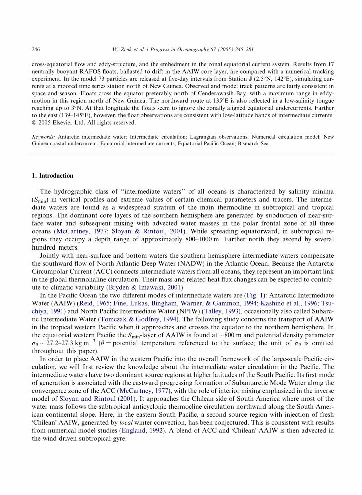
In the Pacific Ocean the two different modes of intermediate waters are (Fig. 1): Antarctic IntermediateWater (AAIW) (Reid, 1965; Fine, Lukas, Bingham, Warner, & Gammon, 1994; Kashino et al., 1996; Tsu-chiya, 1991) and North Pacific Intermediate Water (NPIW) (Talley, 1993), occasionally also called Subarc-tic Intermediate Water (Tomczak & Godfrey, 1994). The following study concerns the transport of AAIWin the tropical western Pacific when it approaches and crosses the equator to the northern hemisphere. Inthe equatorial western Pacific the Smin-layer of AAIW is found at �800 m and potential density parameterrh � 27.2–27.3 kg m�3 (h = potential temperature referenced to the surface; the unit of rh is omittedthroughout this paper).
In order to place AAIW in the western Pacific into the overall framework of the large-scale Pacific cir-culation, we will first review the knowledge about the intermediate water circulation in the Pacific. Theintermediate waters have two dominant source regions at higher latitudes of the South Pacific. Its first modeof generation is associated with the eastward progressing formation of Subantarctic Mode Water along theconvergence zone of the ACC (McCartney, 1977), with the role of interior mixing emphasized in the inversemodel of Sloyan and Rintoul (2001). It approaches the Chilean side of South America where most of thewater mass follows the subtropical anticyclonic thermocline circulation northward along the South Amer-ican continental slope. Here, in the eastern South Pacific, a second source region with injection of fresh�Chilean� AAIW, generated by local winter convection, has been conjectured. This is consistent with resultsfrom numerical model studies (England, 1992). A blend of ACC and �Chilean� AAIW is then advected inthe wind-driven subtropical gyre.
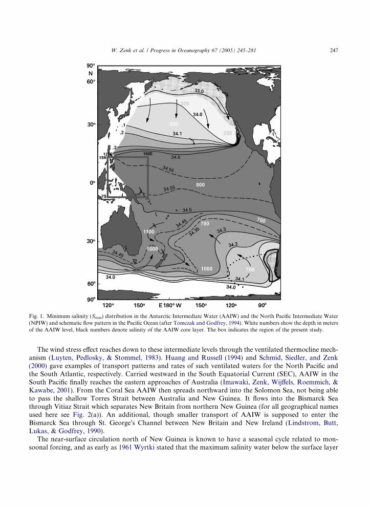
Fig. 1. Minimum salinity (Smin) distribution in the Antarctic Intermediate Water (AAIW) and the North Pacific Intermediate Water(NPIW) and schematic flow pattern in the Pacific Ocean (after Tomczak and Godfrey, 1994). White numbers show the depth in metersof the AAIW level, black numbers denote salinity of the AAIW core layer. The box indicates the region of the present study.
W. Zenk et al. / Progress in Oceanography 67 (2005) 245–281 247
The wind stress effect reaches down to these intermediate levels through the ventilated thermocline mech-anism (Luyten, Pedlosky, & Stommel, 1983). Huang and Russell (1994) and Schmid, Siedler, and Zenk(2000) gave examples of transport patterns and rates of such ventilated waters for the North Pacific andthe South Atlantic, respectively. Carried westward in the South Equatorial Current (SEC), AAIW in theSouth Pacific finally reaches the eastern approaches of Australia (Imawaki, Zenk, Wijffels, Roemmich, &Kawabe, 2001). From the Coral Sea AAIW then spreads northward into the Solomon Sea, not being ableto pass the shallow Torres Strait between Australia and New Guinea. It flows into the Bismarck Seathrough Vitiaz Strait which separates New Britain from northern New Guinea (for all geographical namesused here see Fig. 2(a)). An additional, though smaller transport of AAIW is supposed to enter theBismarck Sea through St. George�s Channel between New Britain and New Ireland (Lindstrom, Butt,Lukas, & Godfrey, 1990).
The near-surface circulation north of New Guinea is known to have a seasonal cycle related to mon-soonal forcing, and as early as 1961 Wyrtki stated that the maximum salinity water below the surface layer
Fig. 2. (a) Basin structure of the lower latitude western Pacific revealed by the 3000 m isobath. The left box denotes the region ofEKE analysis in Fig. 9. The center box indicates the location of the Bismarck Sea, zoomed in the right box. Geographical names asmentioned in this study are give by abbreviated labels: AI = Admiralty Islands incl. Manaus Island, BI = Biak Island,BS = Bismarck Sea, CB = Cenderawasih Bay, CeB = Celebes Basin, {ECB, WCB} = {East, West} Caroline Basin, {EMB,WMB} = {East, West} Mariana Basin, PB = Philippine Basin, H = Halmahera, NB = New Britain, NG = New Guinea, NI = NewIreland, SoS = Solomon Sea, StG = St. George�s Channel, UB = Umboi Island, VS = Vitiaz Strait. (b) Data base used in this study:Historical CTD stations ( Æ ), TROPAC CTD stations (+), WOCE stations (h). The shown RAFOS float displacement vectors endat {large, small} circles indicating {full, shortened} mission lengths according to Table 2. The hexagonal stars denote current metermoorings (Table 4). (c) Trajectories of TROPAC floats at intermediate water levels (for shown RAFOS numbers see Table 3).Launch positions are marked by stars, surfacing positions by circles. Three concentric circles denote positions of sound sourcemoorings. Dashed lines indicate poor tracking due to transmission gaps. Ticks (x) are 10 days apart. Topographic informationoriginates from Smith and Sandwell (1997).
248 W. Zenk et al. / Progress in Oceanography 67 (2005) 245–281
W. Zenk et al. / Progress in Oceanography 67 (2005) 245–281 249
participates in the movements of the surface layer. Tsuchiya (1991) later showed that the flow of thisSmax-water is associated with the New Guinea Coastal Undercurrent (NGCUC). With the NGCUC beingaffected by the monsoon-related seasonal change, the question arises whether seasonal variations can alsobe found in the AAIW layer north of New Guinea. We will attempt to identify such variations.
The second Smin-layer at mid-depth of lower latitudes of the western Pacific reflects NPIW. Its pres-ence is most noticeable in the northeastern corner of the Pacific (Fig. 1). Slow advection, mainly alongisopycnals that deepen towards the center of the subtropical gyre, is related to the anticyclonic wind-dri-ven circulation. Vertical mixing causes a steady increase of the core salinity. The NPIW core is foundbetween 500 and 800 m depth in the North Equatorial Current (NEC) and reaches the tropical westernPacific between 250 and 400 m near the equator (Kashino, Watanabe, Herunadi, Aoyama, & Hartoyo,1999), with typical minimum salinity values of Smin < 34.5. At �15�N the NEC bifurcates at the Philip-pine shelf with the southern limb feeding the southward Mindanao Current. Approaching the CelebesSea NPIW undergoes a cyclonic loop. Portions of modified NPIW leave the Pacific in the IndonesianThroughflow in the form of intrusions, passing Makassar Strait southwestward (Sprintall, Wijffels,Chereskin, & Bray, 2002). The remaining NPIW is advected eastward with the Northern SubsurfaceCountercurrent (NSCC) (Fine et al., 1994; Bingham & Lukas, 1995). NPIW does not appear to crossthe equator to the south. The core of NPIW in the western tropical Pacific typically lies aroundrh = 26.55. The state of knowledge on intermediate waters in the Pacific Ocean was summarized in moredetail by Hanawa and Talley (2001).
The importance of the interhemispheric exchange of intermediate waters for the water mass inventory inthe western Pacific was demonstrated in the model of McCreary and Lu (2001). Bingham and Lukas (1995)inferred pathways of intermediate waters (defined by 25.5 < rh < 27.5) in the western equatorial Pacificbased on hydrographic observations. Their summary suggests the principal path of AAIW to cross theequator along the continental slope, merging with some additional northward flow around 143�E. The dataset used in their study, however, did not cover the equatorial transition region off the northwestern coast ofNew Guinea. Here, we use additional data to determine the location and the flow characteristics in the wes-tern equatorial crossing zone.
In addition to the analysis of in-situ ocean data, results from numerical experiments with a global high-resolution model are presented to provide a better understanding of the observational results. Since theocean observations are limited in space and time, numerical model experiments with their complete spatialand temporal coverage may help to provide a better insight into the circulation at a wide range of scalesfrom mesoscale to basin-scale. The model results are first compared with the observed data for validation,and then the model time-mean and seasonal variations of currents and salinity are discussed. Bi-monthlyplots of model salinity and velocity at the AAIW level provide information on the pathways of the low-salinity waters. The results from a particle-tracking experiment are also presented in order to comparethe model flow with observed float trajectories, providing a more comprehensive view of the pathwaysof AAIW in the western equatorial Pacific Ocean.
2. Observational and model data set
2.1. Hydrography and vessel-mounted acoustic Doppler profiling
The circulation of AAIW in the Bismarck Sea and in the western equatorial Pacific between 120�E and160�E (cf. box in Fig. 1) was one of the main topics of TROPAC, the tropical Pacific expedition conductedon the German research vessel SONNE (10 October to 19 November 1996) with follow-up float observa-tions and joint Japanese-German moored observations. The data sets were presented by Siedler and Zenk(1997). Near-surface data from TROPAC were used by Ioualalen, Siedler, Zenk, Henin, and Picaut (2000)
250 W. Zenk et al. / Progress in Oceanography 67 (2005) 245–281
to study the upper-ocean changes in relation to El Nino, and Siedler, Holfort, Zenk, Muller, and Csernok(2004) used the data in a study of deep and bottom waters in the region. Here, the water between these twostrata will be examined.
While the key data sets in the present study result from TROPAC, we also use hydrographic data setsfrom other sources. In particular, the Japan Agency for Marine-Earth Science and Technology (JAMS-TEC) carried out ten hydrographic cruises north of New Guinea from 1994 to 2000 aboard R/V KAIYOunder the TOCS (Tropical Ocean Climate Study) project (Table 1). During TOCS, CTD and XCTD castswere acquired using a Sea Bird CTD profiler and XCTD probes (made by Tsurumi Seiki Co. Ltd.). Datawere collected north of New Guinea, particularly along the 142�E line between the New Guinea coast andthe equator (Kashino et al., 2001). The selected hydrographic data sets are summarized in Table 1; stationpositions are shown in Fig. 2(b).
For the TROPAC observations a Neil Brown CTD profiler with rosette sampler was used. The majorityof profiles reached the bottom or to pmax = 6000 dbar when deeper. Here, we are only interested in theupper 1000 m. The profiling data were processed in accordance with specifications of the World Ocean Cir-culation Experiment (WOCE). Salinity was checked and recalibrated by laboratory salinometer values ob-tained from rosette samples. For pressure, temperature and salinity of all TROPAC CTD observations weestimate accuracies of at least ±2 dbar, ±2 mK, and ±0.003 (psu, practical salinity units), respectively.
The two long TROPAC CTD sections are located between 143�E and 150�E. They reach from the regionnorth of 8�N to the coastline of New Guinea. An additional short quasi-meridional CTD section along146�E was taken in the Bismarck Sea (Siedler & Zenk, 1997). The hydrographic data sets are supplementedby high-quality WOCE stations (Section P10) and data from the National Oceanographic Data Center(http://www.nodc.noaa.gov/).
Table 1Hydrographic data sets
Source Period Data type
WHP-P04 1989 CTD, bottleCOARE EQ-1 1992 CTD, bottleWHP-PR24 1992 CTD, bottleCOARE EQ-2 1993 CTD, bottleWHP-P10 1993 CTD, bottleCOARE EQ-3 1994 CTD, bottleWHP-P09 1994 CTD, bottleTROPAC/FS SONNE 1996 CTD, bottleWHP-P08 1996 CTD, bottleR/V Franklin 1985–1997 CTD
JAMSTECTOCS cruises (R/V KAIYO)Boreal summerKY9505 Jul 1995 CTD, shipboard ADCP (75 kHz)KY9606 Jul 1996 CTD, shipboard ADCP (75 kHz)KY9709 Aug 1997 CTD, shipboard ADCP (75 kHz)KY9810 Sep 1998 CTD, shipboard ADCP (75 kHz)KY0006 Sep 2000 CTD, XCTD, shipboard ADCP (38 kHz)
Boreal winterKY9406 Jan 1995 CTD, shipboard ADCP (75 kHz)KY9601 Feb 1996 CTD, shipboard ADCP (75 kHz)KY9702 Feb 1997 CTD, shipboard ADCP (75 kHz)KY9801 Jan 1998 CTD, shipboard ADCP (75 kHz)KY9901 Feb 1999 CTD, XCTD, shipboard ADCP (75 kHz)

W. Zenk et al. / Progress in Oceanography 67 (2005) 245–281 251
Current velocity data using the shipboard acoustic Doppler current profiler (ADCP) onboard theKAIYO were also obtained during the TOCS cruises. A vessel-mounted narrow-band 75 kHz ADCP man-ufactured by RD Instruments (measurement depth: 600 m) was used until cruise KY9901. An Ocean Sur-
veyer II-38 kHz model (1000 m) collected data during cruise KY0006.
2.2. Floats
A total of 20 expendable quasi-isobaric RAFOS floats (Rossby, Dorson, & Fontain, 1986; Konig &Zenk, 1992) were deployed from FS SONNE during TROPAC (Tables 2 and 3). The floats were built atthe Institut fur Meereskunde (IfM), Kiel, and pre-ballasted in the IfM pressure vessel. Ballast weight finetuning was carried out immediately before each deployment on the basis of local CTD profiles targetingthe float depths to the AAIW core (typically 800–900 m).
The floats were tracked acoustically by four moored sound sources emitting 12-hourly coded signals of80 s duration. In Fig. 2(c), we present a graphical update of List 6.5 of the cruise report (Siedler & Zenk,1997). It shows deployment (stars) and surfacing (circles) positions of the floats together with the positionsof moored sound sources (concentric circles). The majority of floats immediately off New Guinea traveledwestward. With reference to the later discussion note the collection of tracks near 135�E indicating cross-equatorial motion. Farther north both eastward and westward zonal tracks are seen in the equatorialregion.
An inventory of float data including mission depths is presented in Table 3. In three cases (RAFOSnumbers 179, 188, 189) instruments surfaced prematurely after almost one-year missions. No attempt wasmade to extrapolate their mission to the originally intended duration of 538 days. Simultaneous overall
Table 2RAFOS float inventory
RAFOSno
Launch1996
Surfacedate
Missionday
Dist, km Displ Spd,cm s�1
Launch latitude(�N or �S)
Launchlongitude(�E)
Surfacelatitude(�N or �S)
Surfacelongitude(�E)
171 18 Oct 13 Feb 1997 118 103 1.00 11.449 144.966 11.704 145.874172 18 Oct 5 Apr 1998 534 990 2.15 11.934 145.000 12.908 154.074173 18 Oct a 12.417 144.994 a a
174 17 Oct 7 Apr 1998 537 1028 2.22 12.900 145.000 11.793 154.412175 5 Nov 24 Apr 1998 535 2528 5.47 �0.849 150.167 7.967 129.104177 6 Nov 28 Apr 1998 538 2438 5.25 �2.150 150.167 �5.338 171.952178 6 Nov 28 Apr 1998 538 92 0.20 �2.517 149.600 �3.223 150.040179 6 Nov 11 Sep 1997 309 284 1.07 �2.807 149.399 �4.796 151.018180 7 Nov a �4.475 149.088 a a
181 8 Nov 8 Nov 1996 �1 4 – �5.525 147.537 �5.556 147.525187 7 Nov 30 Apr 1998 538 1438 3.09 �5.722 147.455 �1.025 135.357188 9 Nov 30 Oct 1997 355 1588 5.18 �4.008 145.290 0.178 131.598189 11 Nov 20 Sep 1997 313 932 3.45 �3.133 143.000 1.506 136.002190 11 Nov 4 May 1998 538 1541 3.31 �2.500 143.000 4.925 131.255191 12 Nov 5 May 1998 539 937 2.01 �1.000 143.000 3.702 135.987192 12 Nov 5 May 1998 538 1203 2.59 �0.022 142.825 5.981 133.765193 13 Nov 5 May 1998 537 4022 8.66 2.000 142.484 �0.047 178.669194 14 Nov 6 May 1998 537 824 1.78 3.989 142.352 3.970 134.911197 16 Nov 9 May 1998 538 701 1.51 6.001 138.501 8.191 132.532198 17 Nov 10 May 1998 538 1190 2.56 7.601 137.534 5.919 148.195
Distance between launch and surfacing location (Dist), displacement speed (Displ Spd). Two floats were lost.a No show instrument.
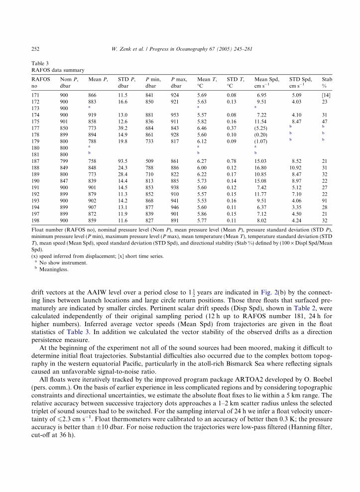
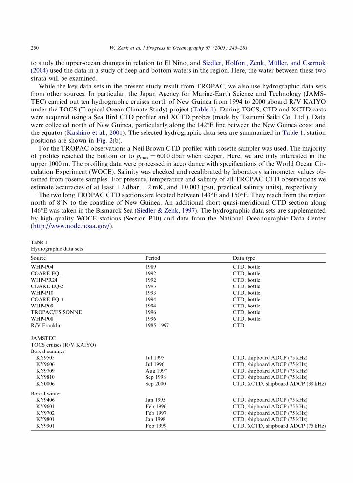
Table 3RAFOS data summary
RAFOSno
Nom P,dbar
Mean P, STD P,dbar
P min,dbar
P max,dbar
Mean T,�C
STD T,�C
Mean Spd,cm s�1
STD Spd,cm s�1
Stab%
171 900 866 11.5 841 924 5.69 0.08 6.95 5.09 [14]172 900 883 16.6 850 921 5.63 0.13 9.51 4.03 23173 900 a a a
174 900 919 13.0 881 953 5.57 0.08 7.22 4.10 31175 901 858 12.6 836 911 5.82 0.16 11.54 8.47 47177 850 773 39.2 684 843 6.46 0.37 (5.25) b b
178 899 894 14.9 861 928 5.60 0.10 (0.20) b b
179 800 788 19.8 733 817 6.12 0.09 (1.07) b b
180 800 a a a
181 800 b b b
187 799 758 93.5 509 861 6.27 0.78 15.03 8.52 21188 849 848 24.3 788 886 6.00 0.12 16.80 10.92 31189 800 773 28.4 710 822 6.22 0.17 10.85 8.47 32190 847 839 14.4 813 885 5.73 0.14 15.08 8.97 22191 900 901 14.5 853 938 5.60 0.12 7.42 5.12 27192 899 879 11.3 852 910 5.57 0.15 11.77 7.10 22193 900 902 14.2 868 941 5.53 0.16 9.51 4.06 91194 899 907 13.1 877 946 5.60 0.11 6.37 3.35 28197 899 872 11.9 839 901 5.86 0.15 7.12 4.50 21198 900 859 11.6 827 891 5.77 0.11 8.02 4.24 32
Float number (RAFOS no), nominal pressure level (Nom P), mean pressure level (Mean P), pressure standard deviation (STD P),minimum pressure level (P min), maximum pressure level (P max), mean temperature (Mean T), temperature standard deviation (STDT), mean speed (Mean Spd), speed standard deviation (STD Spd), and directional stability (Stab %) defined by (100 · Displ Spd/MeanSpd).(x) speed inferred from displacement; [x] short time series.a No show instrument.b Meaningless.
252 W. Zenk et al. / Progress in Oceanography 67 (2005) 245–281
drift vectors at the AAIW level over a period close to 1 12years are indicated in Fig. 2(b) by the connect-
ing lines between launch locations and large circle return positions. Those three floats that surfaced pre-maturely are indicated by smaller circles. Pertinent scalar drift speeds (Disp Spd), shown in Table 2, werecalculated independently of their original sampling period (12 h up to RAFOS number 181, 24 h forhigher numbers). Inferred average vector speeds (Mean Spd) from trajectories are given in the floatstatistics of Table 3. In addition we calculated the vector stability of the observed drifts as a directionpersistence measure.
At the beginning of the experiment not all of the sound sources had been moored, making it difficult todetermine initial float trajectories. Substantial difficulties also occurred due to the complex bottom topog-raphy in the western equatorial Pacific, particularly in the atoll-rich Bismarck Sea where reflecting signalscaused an unfavorable signal-to-noise ratio.
All floats were iteratively tracked by the improved program package ARTOA2 developed by O. Boebel(pers. comm.). On the basis of earlier experience in less complicated regions and by considering topographicconstraints and directional uncertainties, we estimate the absolute float fixes to lie within a 5 km range. Therelative accuracy between successive trajectory dots approaches a 1–2 km scatter radius unless the selectedtriplet of sound sources had to be switched. For the sampling interval of 24 h we infer a float velocity uncer-tainty of 62.3 cm s�1. Float thermometers were calibrated to an accuracy of better then 0.3 K; the pressureaccuracy is better than ±10 dbar. For noise reduction the trajectories were low-pass filtered (Hanning filter,cut-off at 36 h).
Table 4Moored observations
Mooring–InstrDepth, m Launch date Recovery date Water depth, m Latitude, �N or �S Longitude, �E
J�519
} 6 Sep 1998 14 Nov 1999 3453 �2.468 141.978J�733J�897J�1061V371–647 12 Oct 1996 8 Mar 1998 4720 11.428 138.727V374–740 27 Oct 1996 4 Mar 1998 5010 8.643 150.948V375–800 14 Nov 1996 16 Jul 1998 3000 2.833 142.355V376–790 sound source only 16 Nov 1996 15 Jul 1998 3888 4.322 138.640
W. Zenk et al. / Progress in Oceanography 67 (2005) 245–281 253
The averages of all targeted4 float pressures and the recorded pressures (Table 3) were 867.1 and854.1 dbar, respectively. The difference amounts to5 19.0 (±23.7) dbar. It remains unclear why the floatswere systematically ballasted too light. The most likely candidate is the uncertainty in the determinationof the floats� compressibility. Also, the laboratory ballasting procedure requires a pressure tank free of ver-tical thermal gradients which is difficult to maintain under present conditions in the IfM facilities.
2.3. Moorings
Conventional Aanderaa current meters with mechanical rotors were moored from FS SONNE duringthe TROPAC cruise in October/November 1996 and were recovered in March 1998 with the Japaneseresearch vessel HAKUHO MARU (Siedler & Zenk, 1997; Siedler et al., 2004). In addition, current metersfrom the IfM were placed in a mooring (called ‘‘J’’ here) supplied by JAMSTEC from September 1998 toNovember 1999, at levels close to the low-salinity core of the AAIW north of the New Guinea coast at2.5�S, 142�E. JAMSTEC has maintained a time series mooring there with an upward looking 150 kHzADCP by RD Instruments at a depth around 260 m since 1995 (Ueki, Kashino, & Kuroda, 2003). Thepositions of the moorings are indicated in the map (Fig. 2(b)) and the details of the positions, depthsand dates are summarized in Table 4. Basic Eulerian statistics are compiled in Table 5.
2.4. Model experiments
We use model output to complement the observed AAIW results. The JAMSTEC high-resolution model(Ishida, Kashino, Mitsudera, Yoshioka, & Kadokura, 1998) is based on the Modular Ocean Model version2 (Pacanowski & Philander, 1981; Pacanowski, 1995). The domain is zonally global between 75�S and 75�Nwith horizontal grid spacing of 1/4� in both latitude and longitude and 55 levels in the vertical. The verticalgrid spacing increases smoothly from 10 m at the top level to about 50 m near the AAIW layer, and 400 mat the bottom (6000 m). The model topography is derived from the NOAA National Geophysical DataCenter data set (ETOPO5) with a 5 0 latitude–longitude resolution. A Gaussian spatial smoother with influ-ence radii of 1/2� (about 55 km at the equator) above 1000 m depth and smoothly increasing to 1� at6000 m depth is applied to the ETOPO5 topography.
The model is spun up from a state of rest with temperature and salinity initialized by the annual averageLevitus (1982) climatology. Heat and freshwater fluxes are implemented by linear relaxation of surfacetemperature and salinity in the model toward the Levitus climatology with a restoring time scale of 6 days.
4 Pressure at the AAIW core layer as determined by individual pre-launch CTD stations.5 From here on all Xi(±Yi) indicates the standard deviation Yi from a mean value Xi.
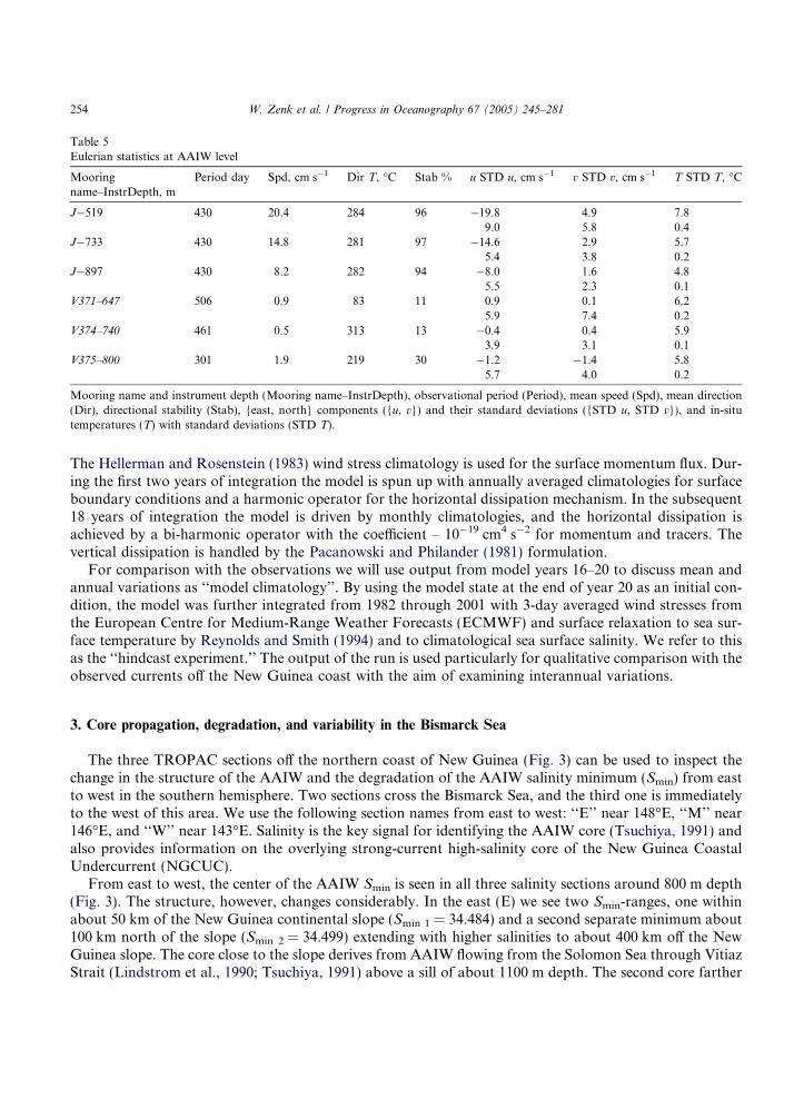
Table 5Eulerian statistics at AAIW level
Mooringname–InstrDepth, m
Period day Spd, cm s�1 Dir T, �C Stab % u STD u, cm s�1 v STD v, cm s�1 T STD T, �C
J�519 430 20.4 284 96 �19.8 4.9 7.89.0 5.8 0.4
J�733 430 14.8 281 97 �14.6 2.9 5.75.4 3.8 0.2
J�897 430 8.2 282 94 �8.0 1.6 4.85.5 2.3 0.1
V371–647 506 0.9 83 11 0.9 0.1 6.25.9 7.4 0.2
V374–740 461 0.5 313 13 �0.4 0.4 5.93.9 3.1 0.1
V375–800 301 1.9 219 30 �1.2 �1.4 5.85.7 4.0 0.2
Mooring name and instrument depth (Mooring name–InstrDepth), observational period (Period), mean speed (Spd), mean direction(Dir), directional stability (Stab), {east, north} components ({u, v}) and their standard deviations ({STD u, STD v}), and in-situtemperatures (T) with standard deviations (STD T).
254 W. Zenk et al. / Progress in Oceanography 67 (2005) 245–281
The Hellerman and Rosenstein (1983) wind stress climatology is used for the surface momentum flux. Dur-ing the first two years of integration the model is spun up with annually averaged climatologies for surfaceboundary conditions and a harmonic operator for the horizontal dissipation mechanism. In the subsequent18 years of integration the model is driven by monthly climatologies, and the horizontal dissipation isachieved by a bi-harmonic operator with the coefficient – 10�19 cm4 s�2 for momentum and tracers. Thevertical dissipation is handled by the Pacanowski and Philander (1981) formulation.
For comparison with the observations we will use output from model years 16–20 to discuss mean andannual variations as ‘‘model climatology’’. By using the model state at the end of year 20 as an initial con-dition, the model was further integrated from 1982 through 2001 with 3-day averaged wind stresses fromthe European Centre for Medium-Range Weather Forecasts (ECMWF) and surface relaxation to sea sur-face temperature by Reynolds and Smith (1994) and to climatological sea surface salinity. We refer to thisas the ‘‘hindcast experiment.’’ The output of the run is used particularly for qualitative comparison with theobserved currents off the New Guinea coast with the aim of examining interannual variations.
3. Core propagation, degradation, and variability in the Bismarck Sea
The three TROPAC sections off the northern coast of New Guinea (Fig. 3) can be used to inspect thechange in the structure of the AAIW and the degradation of the AAIW salinity minimum (Smin) from eastto west in the southern hemisphere. Two sections cross the Bismarck Sea, and the third one is immediatelyto the west of this area. We use the following section names from east to west: ‘‘E’’ near 148�E, ‘‘M’’ near146�E, and ‘‘W’’ near 143�E. Salinity is the key signal for identifying the AAIW core (Tsuchiya, 1991) andalso provides information on the overlying strong-current high-salinity core of the New Guinea CoastalUndercurrent (NGCUC).
From east to west, the center of the AAIW Smin is seen in all three salinity sections around 800 m depth(Fig. 3). The structure, however, changes considerably. In the east (E) we see two Smin-ranges, one withinabout 50 km of the New Guinea continental slope (Smin 1 = 34.484) and a second separate minimum about100 km north of the slope (Smin 2 = 34.499) extending with higher salinities to about 400 km off the NewGuinea slope. The core close to the slope derives from AAIW flowing from the Solomon Sea through VitiazStrait (Lindstrom et al., 1990; Tsuchiya, 1991) above a sill of about 1100 m depth. The second core farther
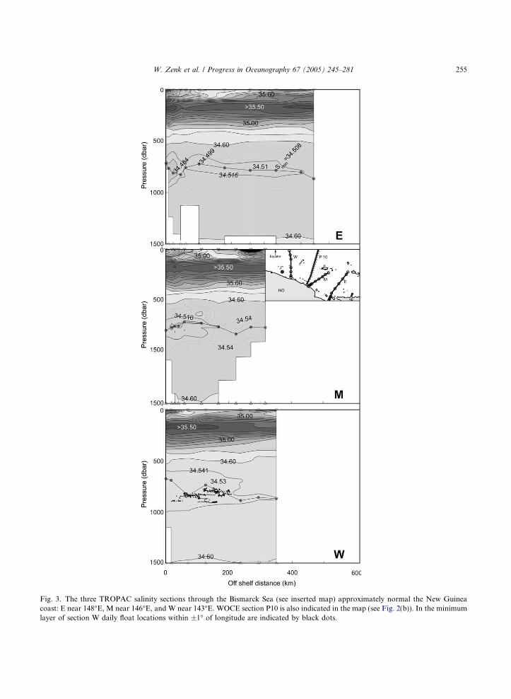
Fig. 3. The three TROPAC salinity sections through the Bismarck Sea (see inserted map) approximately normal the New Guineacoast: E near 148�E, M near 146�E, and W near 143�E. WOCE section P10 is also indicated in the map (see Fig. 2(b)). In the minimumlayer of section W daily float locations within ±1� of longitude are indicated by black dots.
W. Zenk et al. / Progress in Oceanography 67 (2005) 245–281 255
256 W. Zenk et al. / Progress in Oceanography 67 (2005) 245–281
off-shore is situated north of the line given by New Britain and Umboi Island (see Fig. 2(a)) which are con-nected by a submarine ridge. The Smin-layer appears to lie above the slope towards the center of theBismarck Sea.
It will be shown below (see also Table 2) that the displacement of float 178 is consistent with the offshoreAAIW core having its source in St. George�s Channel (sill depth about 1000 m). The AAIW probablyarrives at this strait between New Britain and New Ireland on a path along the southeastern slope ofNew Britain in the Solomon Sea, and continues to section E following a cyclonic (clock-wise) path inthe Bismarck Sea. At M the two cores have merged, although interleaving and patchiness suggests incom-plete mixing. The salinity of the core (SminM = 34.492) is in-between the salinities of the former two cores.At W we find a core similar in size, however with slightly higher salinity (SminW = 34.502), due to entrain-ment and mixing.
With the low-salinity core of AAIW-influenced water changing in structure, size and salinity, it isinstructive to consider the systematic increase of the salt content in the cores by examining the anomalyof salt content relative to the lowest minimum salinity S0E = Smin1. We calculate the following integralfor the three quasi-synoptic observational sections:
Fig. 4.(n), anregionmarke
Msn=Dl ¼ qZ Z
core
Snðx; zÞ � S0E½ �dx dz;
whereMsn/Dl is the AAIW excess of salt content relative to the base S0E (per unit length) and n an index forsections {E, M, W}. The cross-section of the individual core is defined by a certain isohaline called Slim n.The coordinates x and z are the horizontal (approximately normal to the coast of New Guinea) and verticalcoordinates, respectively. The density q is approximated by 103 kg m�3.
Salt content anomaly in the deep AAIW tongue enclosed by selected isolines of minimal salinity (Slim n) for sections E (x), Md W (v). Note the similarity between E and M. Section W is directly influenced by more saline water masses from equatorials, leaving only minor traces of S < SlimW in the water column of W. Sample values at 50 and 100 km off-shelf distance ared by circled stars (for details see text).
W. Zenk et al. / Progress in Oceanography 67 (2005) 245–281 257
How can we define the cross-sections of the cores? We have to find a definition which locates the outerboundary of the salinity gradient region related to the core. We therefore assume that the core is best de-scribed by the closed contour lines (Slim n = {34.516, 34.510, 34.541}) indicating the bonds for the AAIWcore in the three sections. The resulting integrals are given in Fig. 4. The cumulative salt anomalies increasewith off-shelf distance. The values at {E, M} are very similar and indistinguishable within the given errorbars where uncertainties were obtained by changing the salinity of the integration boundaries by ±0.01.Anomalies at {E, M} and W increase with growing distance. As approximate indicators for the changesin the near-shelf core and farther north near the core�s edge, the values at 50 and 100 km off-shelf distanceare marked in Fig. 4 by circled stars. The salt anomalies increase from the mean of sections {E, M} to sec-tion W by about 70% at 50 km and by about 40% at 100 km distance to the continental slope. This providesa measure of the salt increase in the AAIW core by mixing with surrounding saltier waters when the corepropagates from the Bismarck Sea to the oceanic waters of the Caroline Basins. The relative salt contentchanges more strongly in the near-shelf core than near the northern boundary of the core. Additional sen-sitivity tests with varying base salinities S0n taken from the cores of the other sections yielded no significantdeviations (<5%) from the results in Fig. 4.
At depth levels further above (around 200 m) in the three sections we recognize a salinity maximum offthe New Guinea slope in Fig. 3 marking the strong-current core of the NGCUC (Tsuchiya, 1968;Lindstrom et al., 1987; Butt & Lindstrom, 1994). It was shown by Tsuchiya, Lukas, Fine, Firing, and Lind-strom (1989) that this core is characterized by high salinity and oxygen concentrations and by low nutrientcontent and that it can be traced back to the subtropical South Pacific. Wijffels et al. (1998) concluded thatthis South Pacific Subtropical Water arrives from the South Pacific subtropical gyre in a westward flow.The transport of the NGCUC water to the Bismarck Sea through Vitiaz Strait and St. George�s Channelwas documented by Lindstrom et al. (1990). For a review on NGCUC investigations we refer to Cresswell(2000). An example of the zonal component of an ADCP section at 142�E between New Guinea and theequator is presented in Fig. 5. We note that he high-salinity core has a similar horizontal scale as thelow-salinity AAIW core.
We will next inspect the Lagrangian data from the Bismarck Sea (RAFOS floats no. 178, 179, 187–192 inFig. 2(c)). One of the floats (187) was launched in Vitiaz Strait. It showed a series of peculiar jumps in its pres-sure record. Apparently it hit the bottom after about one year of free drift along theNewGuinea slope, endingits mission at the lowest pressure of its record (Table 3). Eight floats were chosen as typical indicators for theNGCUC(seeFig. 2(b) and (c)).Wenote that thiswell developed deepboundary current along theNewGuineaslope at AAIW level was primarily observed in boreal summer (April–September 1997).
The statistical parameters in Table 6 show that differences between medians (umed, vmed) and mean val-ues (um, vm) for the zonal and meridional velocity estimates rarely exceeded 2 cm s�1. Within the chosenperiods these floats were swiftly advected to the northwest, apparently under strong topographic control atthe continental slope off New Guinea. In three cases speeds exceeded 20 cm s�1 over month-long periods,with standard deviations of about 50%. The ensemble average speed is 18.6 (±5.1) cm s�1. The high direc-tional stabilities of P85% (last column in Table 6) indicate jet-like advection. They are significantly higherthan those of the record-long statistics in Table 3 (last column). This result is not surprising because Table 6presents results for much longer time periods that occasionally include eddy-dominated trajectories. Themean kinetic energy MKE = 1/2 (um2 + vm2) of the NGCUC lies in the range (130–200) cm2 s�2, andthe ensemble MKE for these floats is 137 cm2 s�2.
Unfortunately we were not able to track in detail three of the floats that had been deployed in theBismarck Sea (178, 179, 181). Nevertheless, we obtained the surfacing locations for floats 178 and 179(see Fig. 2(b) and (c)). Both total float displacements are not inconsistent with a hypothetical cyclonic(clockwise) circulation in the Bismarck Sea, leading into the boundary currents off New Guinea farther west(floats 187–189). It thus corresponds to the conclusions on the AAIW core from hydrography which weregiven above. The interior cyclone seems to be confined by the ridge between New Ireland and the Admiralty
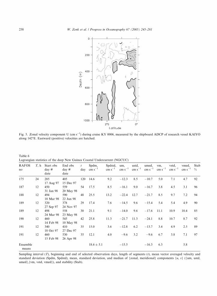
Table 6Lagrangian statistics of the deep New Guinea Coastal Undercurrent (NGCUC)
RAFOSno
T, h Start obsday #date
End obsday #date
t
daySpdm,cm s�1
Spdstd,cm s�1
um,cm s�1
ustd,cm s�1
umed,cm s�1
vm,cm s�1
vstd,cm s�1
vmed,cm s�1
Stab%
175 24 285 405 120 14.6 9.2 �12.3 8.5 �10.7 5.0 7.1 4.7 9217 Aug 97 15 Dec 97
187 12 450 559 54 17.5 8.5 �16.1 9.0 �16.7 3.8 4.5 3.1 9631 Jan 98 20 May 98
188 12 494 590 48 25.5 13.2 �22.4 12.7 �21.7 8.5 9.7 7.2 9418 Mar 98 22 Jun 98
189 12 320 378 29 17.4 7.6 �14.5 9.6 �15.4 5.4 5.4 4.9 9027 Sep 97 24 Nov 97
189 12 498 558 30 21.1 9.1 �14.0 9.6 �17.6 11.1 10.9 10.4 8524 Mar 98 23 May 98
190 12 460 545 42 25.8 11.3 �21.7 11.3 �24.1 8.8 10.7 8.7 9214 Feb 98 10 May 98
191 12 340 410 35 15.0 3.6 �12.8 6.2 �13.7 3.4 4.9 2.5 8918 Oct 97 27 Dec 97
191 12 460 530 35 12.1 4.0 �9.6 3.2 �9.6 6.7 3.8 7.1 9715 Feb 98 26 Apr 98
Ensemblemeans
18.6 ± 5.1 �15.5 �16.3 6.3 5.8
Sampling interval (T), beginning and end of selected observation days, length of segments (t), mean vector averaged velocity andstandard deviation (Spdm, Spdstd), mean, standard deviation, and median of {zonal, meridional} components {u, v} ({um, ustd,umed},{vm, vstd, vmed}), and stability (Stab).
Fig. 5. Zonal velocity component U (cm s�1) during cruise KY 0006, measured by the shipboard ADCP of research vessel KAIYOalong 142�E. Eastward (positive) velocities are hatched.
258 W. Zenk et al. / Progress in Oceanography 67 (2005) 245–281

Salinity
Pot
entia
ltem
pera
ture
(deg
C)
27.0
26.9
27.2
27.1
27.3
27.4
34.42 34.44 34.46 34.48 34.50 34.52 34.54 34.56 34.58
8.0
7.5
7.0
6.5
6.0
5.5
5.0
4.5
4.0
Fig. 6. Potential temperature–salinity relations in the AAIW Smin layer from CTD measurements near the position of the currentmeter time series station J (2.5�S, 142.0�E; see Table 4) during the ten TOCS cruises (see Table1 1). Solid lines give data from borealsummer, dotted from winter. Contours indicate potential density rh.
W. Zenk et al. / Progress in Oceanography 67 (2005) 245–281 259
Islands (Fig. 2(a)) in the north. Float 175, on the northern side of the ridge that includes the AdmiraltyIslands, drifted westward, i.e. in the opposite direction of the suggested cyclonic circulation in the interiorBismarck Sea.
We estimate the transports in the AAIW core at sections {E, M}, using the float data together withhydrographic data. The total transport of the NGCUC water to the Bismarck Sea through Vitiaz Straitand St. George�s Channel was presented on the basis of moored current meter and ADCP data sets byLindstrom et al. (1990). If we consider the prime Smin1 core from the Vitiaz Strait in section E and applythe averaged float speed in the intermediate boundary current regime from Table 6 (see above: 18.6 (±5.1)cm s�1), the integration yields 2.2 (±0.6) Sv6 for the core transport enclosed by the isohalineSlimE = 34.516. The same type of calculation for section M, but with a core width of 120 km andSlimM = 34.510, results in 5.1 (±1.4) Sv. We attribute the more than doubling of the transport in the AAIWcore to entrainment as discussed above.
We want to remind the reader that our estimates represent only the deepest portions of the NGCUC andalso required simplified assumptions for the structure of the current field. They cannot be compared directlywith transports for the whole NGCUC (8–14 Sv), including the speed maximum (59 cm s�1) at 200 m
6 1 Sv = 106 m3 s�1.
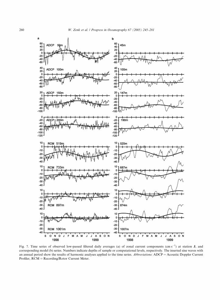
Fig. 7. Time series of observed low-passed filtered daily averages (a) of zonal current components (cm s�1) at station J, andcorresponding model (b) series. Numbers indicate depths of sample or computational levels, respectively. The inserted sine waves withan annual period show the results of harmonic analyses applied to the time series. Abbreviations: ADCP = Acoustic Doppler CurrentProfiler, RCM = Recording/Rotor Current Meter.
260 W. Zenk et al. / Progress in Oceanography 67 (2005) 245–281
Table 7Averages (Um and Vm) and standard deviations (Ustd and Vstd) of velocities during boreal winter (January–March, 1999) andsummer (July–September, 1999) at station J situated at 2�300S, 142�E
Depth (m) Winter (January 1 to March 31, 1999) Summer (July 1 to September 30, 1999)
Um Ustd Vm Vstd Um Ustd Vm Vstd
50 9.5 32.8 �8.4 10.9 �36.0 13.4 3.7 7.0200 �48.2 12.3 8.6 8.5 �58.8 13.3 9.3 11.3519 �14.0 7.8 1.4 4.6 �22.3 8.1 3.5 5.2733 �11.9 6.0 1.3 4.1 �13.2 4.6 1.7 3.8897 �4.3 5.4 0.9 2.4 �6.5 5.7 0.5 2.81061 2.4 6.8 0.9 3.0 �1.5 5.0 0.6 3.1
Negative values indicate westward flow. Units in cm/s.
W. Zenk et al. / Progress in Oceanography 67 (2005) 245–281 261
(Tsuchiya, 1968; Lindstrom et al., 1990; Gouriou & Toole, 1993; Butt & Lindstrom, 1994; Saunders, Cow-ard, & de Cuevas, 1999).
It is well known (see history in Lindstrom et al., 1990) that the New Guinea Coastal Current (NGCC) inthe upper 100 m has a seasonal (monsoonal) cycle. Is there a seasonal cycle also in the deeper water massesand currents? When grouping h/S relations for boreal summer and winter (Fig. 6), it becomes obvious thata seasonal change in water mass properties exists even in this intermediate water mass. The typical Smin isabout 34.50 in boreal summer and 34.53 in boreal winter (near rh = 27.22 and h = 5.50 and 5.65 �C, respec-tively). However, fine structure on scales of tens to hundreds of meters is seen in the individual profileswhich probably indicate short-term variability. Dissolved oxygen distributions (not shown) seem to behigher in boreal summer, but the signal is not as clear as it is in salinity.
Eulerian velocities from two years of mooring J measurements at this position also indicate an annualvariation (Fig. 7(a), Fig. 20). The mooring was located slightly off the center of the AAIW core, but def-initely within its northern extension. In Table 7 we present mean current values including their standarddeviations for the periods January–March and July–September. The seasonal current reversal in the NGCCis well recognized at the uppermost level in Fig. 7(a). The NGCUC is a strong current with up to about80 cm s�1 (matching well Gouriou & Toole�s (1993) results from vessel mounted ADCP data, see below)and points westward at 200 m throughout the year. A similar behavior with steadily decreasing magnitudeis found at greater depth down to the AAIW levels, where maximum velocities are about 20 cm s�1. Aver-aged ADCP sections for the upper ocean between the mooring position and the equator were presented byUeki et al. (2003), indicating seasonal variability not only in the NGCC, but also in the NGCUC. The cur-rents at 519 and 733 m depth in Table 7 appear to have a seasonal variation which is almost in phase withthe current reversal in the NGCC.
4. Interhemispheric pathways
It is generally accepted that AAIW is transported equatorward along the western continental slope of thetropical Pacific. Here, we explore the interhemispheric pathways of this watermass on the basis of eddy-resolving float observations and hydrography and compare them with results from the numerical model.
Floats 187–192 were launched south of the equator (see Table 2), and all of them crossed the equator tonorthern latitudes. We noted earlier the group of tracks in Fig. 2(c) in the region of cross-equatorial mo-tion near 135�E north of Biak Island, i.e. off Cenderawasih Bay (see Fig. 2(a)). Closer inspection of thetracks indicates that all of them crossed the equator east of this longitude; none were carried west tothe intersection of the continental slope at the equator. We note that the slope is almost parallel and close

Fig. 8. Observed salinity on density surface r1 = 31.8 corresponding to the averaged depth level of AAIW (rh = 27.1–27.3) in thewestern tropical Pacific. All used hydrographic stations are given by crosses (see Table1 1 and Fig. 2(b)). A total of 2290 CTD stationswere processed.
262 W. Zenk et al. / Progress in Oceanography 67 (2005) 245–281
to the equator between 135�E and 132�E. If the AAIW core crosses the equator east of 135�E there shouldbe a corresponding signal in the salinity minimum distribution. In order to take into account depth vari-ations of isopycnals, we plot the salinity on the isopycnal surface r1 = 31.8 (corresponding to an averagedpressure of 785.7 (±28.0) dbar at 2918 interpolated grid points) in Fig. 8. Data from numerous cruises areused (see Table 1). Low-salinity water is seen all along the northern New Guinea slope, but the center ofthe low-salinity core appears to cross the equator north of Cenderawasih Bay, consistent with the floattrajectories.
In Fig. 9(a) we map the eddy kinetic energy (EKE) distributions inferred from our Lagrangian observa-tions. Box averages (1� · 1� or 111 km · 111 km) are calculated for identifiable interhemispheric pathways,and the data are then objectively analyzed. This procedure has the effect of a filter that preserves the steadyflow while suppressing mesoscale structures and temporal variability (Davis, 1998). Following Hiller andKase (1983) we choose an exponential shape of the covariance function. The boxes appear large enoughto represent mean speeds from several fixes even for high-speed floats. Assuming near-stationarity andhomogeneous statistics in bins we estimate quasi-Eulerian means and standard deviations. In order toensure robust results we define two criteria for box rejection: <3 instruments and 610 float days perbox. The shaded area in Fig. 9(a) represents the area beyond which the error exceeds 40% of the observedvariance. A correlation length of 90 km and a signal-to-noise ratio of 0.25 is chosen iteratively as the opti-mum compromise between spatial resolution and expected accuracy. In general, Fig. 9(a) shows a maxi-mum range of EKE extending from the northern boundary of Cenderawasih Bay to the northwest.Highest EKE values (�140 cm2 s�2) are observed near 3�N, i.e. on the northern shoulder of the NorthernIntermediate Countercurrent (NICC).
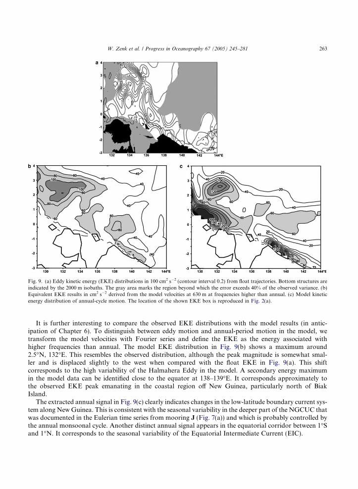
Fig. 9. (a) Eddy kinetic energy (EKE) distributions in 100 cm2 s�2 (contour interval 0.2) from float trajectories. Bottom structures areindicated by the 2000 m isobaths. The gray area marks the region beyond which the error exceeds 40% of the observed variance. (b)Equivalent EKE results in cm2 s�2 derived from the model velocities at 630 m at frequencies higher than annual. (c) Model kineticenergy distribution of annual-cycle motion. The location of the shown EKE box is reproduced in Fig. 2(a).
W. Zenk et al. / Progress in Oceanography 67 (2005) 245–281 263
It is further interesting to compare the observed EKE distributions with the model results (in antic-ipation of Chapter 6). To distinguish between eddy motion and annual-period motion in the model, wetransform the model velocities with Fourier series and define the EKE as the energy associated withhigher frequencies than annual. The model EKE distribution in Fig. 9(b) shows a maximum around2.5�N, 132�E. This resembles the observed distribution, although the peak magnitude is somewhat smal-ler and is displaced slightly to the west when compared with the float EKE in Fig. 9(a). This shiftcorresponds to the high variability of the Halmahera Eddy in the model. A secondary energy maximumin the model data can be identified close to the equator at 138–139�E. It corresponds approximately tothe observed EKE peak emanating in the coastal region off New Guinea, particularly north of BiakIsland.
The extracted annual signal in Fig. 9(c) clearly indicates changes in the low-latitude boundary current sys-tem along NewGuinea. This is consistent with the seasonal variability in the deeper part of the NGCUC thatwas documented in the Eulerian time series from mooring J (Fig. 7(a)) and which is probably controlled bythe annual monsoonal cycle. Another distinct annual signal appears in the equatorial corridor between 1�Sand 1�N. It corresponds to the seasonal variability of the Equatorial Intermediate Current (EIC).
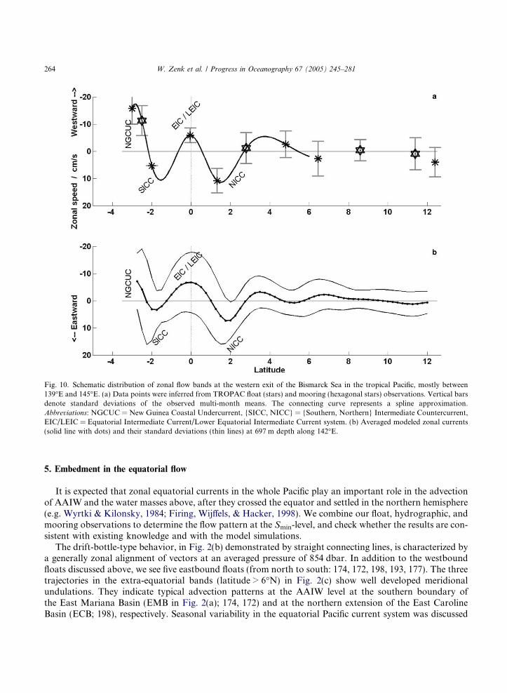
Fig. 10. Schematic distribution of zonal flow bands at the western exit of the Bismarck Sea in the tropical Pacific, mostly between139�E and 145�E. (a) Data points were inferred from TROPAC float (stars) and mooring (hexagonal stars) observations. Vertical barsdenote standard deviations of the observed multi-month means. The connecting curve represents a spline approximation.Abbreviations: NGCUC = New Guinea Coastal Undercurrent, {SICC, NICC} = {Southern, Northern} Intermediate Countercurrent,EIC/LEIC = Equatorial Intermediate Current/Lower Equatorial Intermediate Current system. (b) Averaged modeled zonal currents(solid line with dots) and their standard deviations (thin lines) at 697 m depth along 142�E.
264 W. Zenk et al. / Progress in Oceanography 67 (2005) 245–281
5. Embedment in the equatorial flow
It is expected that zonal equatorial currents in the whole Pacific play an important role in the advectionof AAIW and the water masses above, after they crossed the equator and settled in the northern hemisphere(e.g. Wyrtki & Kilonsky, 1984; Firing, Wijffels, & Hacker, 1998). We combine our float, hydrographic, andmooring observations to determine the flow pattern at the Smin-level, and check whether the results are con-sistent with existing knowledge and with the model simulations.
The drift-bottle-type behavior, in Fig. 2(b) demonstrated by straight connecting lines, is characterized bya generally zonal alignment of vectors at an averaged pressure of 854 dbar. In addition to the westboundfloats discussed above, we see five eastbound floats (from north to south: 174, 172, 198, 193, 177). The threetrajectories in the extra-equatorial bands (latitude > 6�N) in Fig. 2(c) show well developed meridionalundulations. They indicate typical advection patterns at the AAIW level at the southern boundary ofthe East Mariana Basin (EMB in Fig. 2(a); 174, 172) and at the northern extension of the East CarolineBasin (ECB; 198), respectively. Seasonal variability in the equatorial Pacific current system was discussed
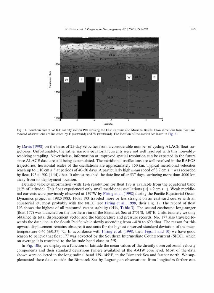
Fig. 11. Southern end of WOCE salinity section P10 crossing the East Caroline and Mariana Basins. Flow directions from float andmoored observations are indicated by E (eastward) and W (westward). For location of the section see insert in Fig. 3.
W. Zenk et al. / Progress in Oceanography 67 (2005) 245–281 265
by Davis (1998) on the basis of 25-day velocities from a considerable number of cycling ALACE float tra-jectories. Unfortunately, the rather narrow equatorial currents were not well resolved with this non-eddy-resolving sampling. Nevertheless, information at improved spatial resolution can be expected in the futuresince ALACE data are still being accumulated. The meridional oscillations are well resolved in the RAFOStrajectories; horizontal scales of the oscillations are approximately 150 km. Typical meridional velocitiesreach up to ±10 cm s�1 at periods of 40–50 days. A particularly high mean speed of 8.7 cm s�1 was recordedby float 193 at 902 (±14) dbar. It almost reached the date line after 537 days, surfacing more than 4000 kmaway from its deployment location.
Detailed velocity information (with 12-h resolution) for float 193 is available from the equatorial band(±2� of latitude). This float experienced only small meridional oscillations (jvj < 2 cm s�1). Weak meridio-nal currents were previously observed at 159�W by Firing et al. (1998) during the Pacific Equatorial OceanDynamics project in 1982/1983. Float 193 traveled more or less straight on an eastward course with anequatorial jet, most probably with the NICC (see Firing et al., 1998, their Fig. 1). The record of float193 shows the highest of all measured vector stability (91%, Table 3). The second eastbound long-ranger(float 177) was launched on the northern rim of the Bismarck Sea at 2�51 0S, 150�E. Unfortunately we onlyobtained its total displacement vector and the temperature and pressure records. No. 177 also traveled to-wards the date line in the South Pacific while slowly ascending from �820 to 690 dbar. The reason for thisupward displacement remains obscure; it accounts for the highest observed standard deviation of the meantemperature 6.46 (±0.37) �C. In accordance with Firing et al. (1998, their Figs. 1 and 10) we have goodreason to believe that float 177 was advected by the Southern Intermediate Countercurrent (SICC), whichon average it is restricted to the latitude band close to 2�S.
In Fig. 10(a) we display as a function of latitude the mean values of the directly observed zonal velocitycomponents and their standard deviations (where available) at the AAIW core level. Most of the datashown were collected in the longitudinal band 139–145�E, in the Bismarck Sea and farther north. We sup-plemented these data outside the Bismarck Sea by Lagrangian observations from longitudes farther east
266 W. Zenk et al. / Progress in Oceanography 67 (2005) 245–281
(150–175�E) where we can reasonably assume large zonal coherence scales. In their analysis Gouriou andToole (1993) were confronted with the same problem when comparing upper layer current observationsfrom 165�E with those of 137�E and 142�E. For the central Pacific they state ‘‘Neglect of difference overa few degrees of longitude is typically easy to justify given the long zonal scales of the equatorial circula-tion. . .’’. As an additional justification we refer to results by Firing et al. (1998) who also found high coher-ence of equatorial current bands between 165�E and 159�W: ‘‘These two sections. . . are separated by 36� oflongitude and a major island chain (the Gilberts), yet they show nearly identical arrangements of zonal cur-rents from 500 to 3500 m’’. The statistical significance of the averages in Fig. 11(a) varies. Data points southof the equator represent ensembles of floats i.e. 175, 187–191 or vertically integrated values (mooring J inTable 5). In other cases subsets of the available trajectories were chosen subjectively, such as float 192 at theequator [recording day 1–65], float 194 [day 450–537], and float 198 [day 215–538].
With respect to our Lagrangian and Eulerian data set the best sampled current (floats: �18.6 (±5.1)cm s�1, mooring: �11.3 (±5.5) cm s�1) hugs the continental slope in the southern Bismarck Sea. It is partof the (north)westward NGCUC/AAIW-core regime off northern New Guinea at the southern boundary inFig. 10. The whole regime was extensively studied by Tsuchiya et al. (1989). Gouriou and Toole (1993)observed the upper core layer of this near-coastal current by a variety of profiling methods. North ofNew Guinea at 2.17�S they found strong westward currents up to 59 (±11) cm s�1 at 200 m depth. Severalfloats indicated the subsurface and intermediate countercurrents near the equator (Tsuchiya, 1975; Firinget al., 1998). East of 150�E (Fig. 10: at 2�S) float 177 gave a rough estimate of the eastward SICC with sub-stantially lower speeds of about +5.3 cm s�1. Its much stronger northern equivalent, the eastward NorthernIntermediate Countercurrent (NICC) (Fig. 10(a): at 2�N) in our data has a mean of 9.3 (±4.4) cm s�1 (float193). Between these two countercurrents, a pronounced westbound flow likely indicative of the EquatorialIntermediate Current (EIC) was recorded by float 192 (�10.1 ± 7.2 cm s�1) (Delcroix & Henin, 1988).For its deeper part Firing et al. (1998) coined a new name: Lower Equatorial Intermediate Current (LEIC).
Fig. 12. Salinity section near 142�E during TROPAC. The depth of the AAIW core layer (Smin) is shown by a white line. The whitevertical dotted line indicates the equator, and the broken line on the right side indicates the location of the zonal shift in the section at4�N. For location see Fig. 2(b).
(psu)(m/s)
4
a b
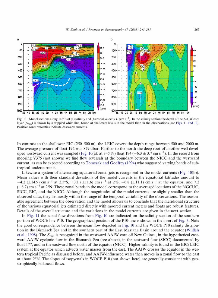
Fig. 13. Model sections along 142�E of (a) salinity and (b) zonal velocityU (cm s�1). In the salinity section the depth of the AAIW corelayer (Smin) is shown by a stippled white line, found at shallower levels in the model than in the observations (see Figs. 11 and 12).Positive zonal velocities indicate eastward currents.
W. Zenk et al. / Progress in Oceanography 67 (2005) 245–281 267
In contrast to the shallower EIC (250–500 m), the LEIC covers the depth range between 500 and 2000 m.The average pressure of float 192 was 879 dbar. Farther to the north the deep root of another well devel-oped westward current was sampled (Fig. 10(a): at 3–6�N) float 194 (�6.3 ± 3.7 cm s�1). In the record frommooring V375 (not shown) we find flow reversals at the boundary between the NICC and the westwardcurrent, as can be expected according to Tomczak and Godfrey (1994) who suggested varying bands of sub-tropical undercurrents.
Likewise a system of alternating equatorial zonal jets is recognized in the model currents (Fig. 10(b)).Mean values with their standard deviations of the model currents in the equatorial latitudes amount to�4.2 (±14.9) cm s�1 at 2.5�S, +3.1 (±11.6) cm s�1 at 2�S, �6.8 (±11.1) cm s�1 at the equator, and 7.2(±6.7) cm s�1 at 2�N. These zonal bands in the model correspond to the averaged locations of the NGCUC,SICC, EIC, and the NICC. Although the magnitudes of the model currents are slightly smaller than theobserved data, they lie mostly within the range of the temporal variability of the observations. The reason-able agreement between the observation and the model allows us to conclude that the meridional structureof the various equatorial jets estimated directly with moored current meters and floats are robust features.Details of the overall structure and the variations in the model currents are given in the next section.
In Fig. 11 the zonal flow directions from Fig. 10 are indicated on the salinity section of the southernportion of WOCE line P10. The geographical position of the P10-line is shown in the insert of Fig. 3. Notethe good correspondence between the mean flow depicted in Fig. 10 and the WOCE P10 salinity distribu-tion in the Bismarck Sea and in the southern part of the East Mariana Basin around the equator (Wijffelset al., 1998). The Smin is recognized in the westward AAIW core off New Guinea, in the hypothetical east-ward AAIW cyclonic flow in the Bismarck Sea (see above), in the eastward flow (SICC) documented byfloat 177, and in the eastward flow north of the equator (NICC). Higher salinity is found in the EIC/LEICsystem at the equator which advects water masses from the east. The AAIW crosses the equator in the wes-tern tropical Pacific as discussed before, and AAIW-influenced water then moves in a zonal flow to the eastat about 2�N. The slopes of isopycnals in WOCE P10 (not shown here) are generally consistent with geo-strophically balanced flows.
268 W. Zenk et al. / Progress in Oceanography 67 (2005) 245–281
6. Comparison of the observational results with the JAMSTEC model
6.1. Mean state and seasonal variability
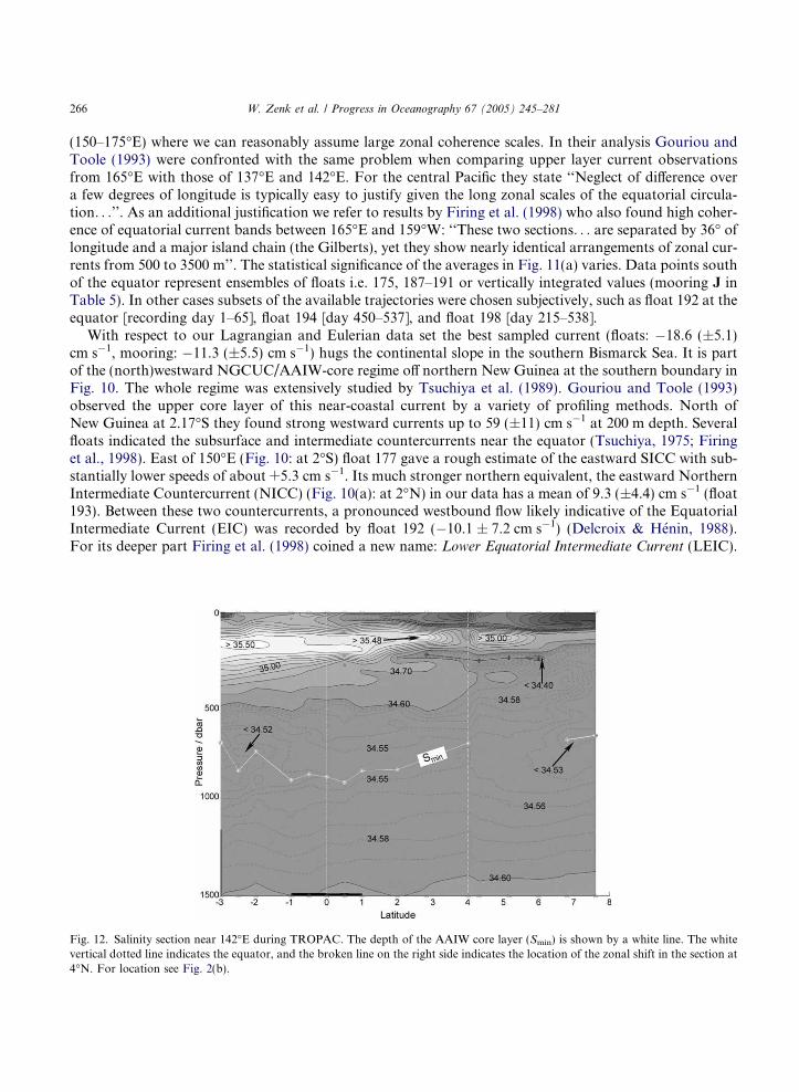
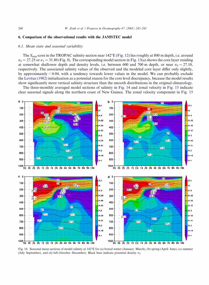
The Smin-core in the TROPAC salinity section near 142�E (Fig. 12) lies roughly at 800 m depth, i.e. aroundrh = 27.25 or r1 = 31.80 (Fig. 8). The corresponding model section in Fig. 13(a) shows the core layer residingat somewhat shallower depth and density levels, i.e. between 600 and 700 m depth, or near rh = 27.10,respectively. The associated salinity values of the observed and the modeled core layer differ only slightly,by approximately < 0.04, with a tendency towards lower values in the model. We can probably excludethe Levitus (1982) initialization as a potential reason for the core level discrepancy, because the model resultsshow significantly more vertical salinity structure than the smooth distributions in the original climatology.
The three-monthly averaged model sections of salinity in Fig. 14 and zonal velocity in Fig. 15 indicateclear seasonal signals along the northern coast of New Guinea. The zonal velocity component in Fig. 15
a b
c d
Fig. 14. Seasonal mean sections of model salinity at 142�E for (a) boreal winter (January–March), (b) spring (April–June), (c) summer(July–September), and (d) fall (October–December). Black lines indicate potential density rh.

a b
c d
Fig. 15. Same as Fig. 14 except for zonal velocity U (cm s�1). Positive zonal velocities indicate eastward currents.
W. Zenk et al. / Progress in Oceanography 67 (2005) 245–281 269
demonstrates that the NGCUC extends from the high-velocity levels near 200 m down to the AAIW core.The NGCUC starts its deep downward extension in boreal spring (April–June). The maximum westward(i.e., equatorward) speed reaches up to 20 cm s�1 in boreal summer (July–September) at the model AAIWlayer. Still faster currents are modeled on the shelf slope off New Guinea for the boreal winter. We furthernote a well developed latitudinal symmetry in the model intermediate countercurrents SICC and NICC atthe 800 m level at the same time. In accordance with the seasonal current fluctuations, the salinity of theselayers oscillates: low in boreal summer and high in winter.
Since the model meridional sections indicate the Smin-layer on rh = 27.10, the horizontal distributions ofsalinity and velocity on that isopycnal surface are examined for comparison with the observations; theannual mean is given in Fig. 16 and monthly means in Figs. 17 and 18. The annual mean salinity section(Fig. 16(a)) clearly indicates two low-salinity sources of the western equatorial Pacific: the NGCUC and theMindanao Current (MC), and also two zonal bands with low salinities at 2�N and 5�N and three bands of
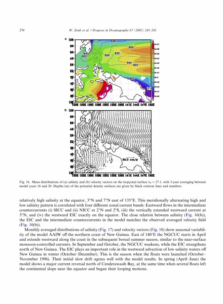
Fig. 16. Mean distributions of (a) salinity and (b) velocity vectors on the isopycnal surface rh = 27.1, with 5-year averaging betweenmodel years 16 and 20. Depths (m) of the potential density surfaces are given by black contour lines and numbers.
270 W. Zenk et al. / Progress in Oceanography 67 (2005) 245–281
relatively high salinity at the equator, 3�N and 7�N east of 135�E. This meridionally alternating high andlow salinity pattern is correlated with four different zonal current bands: Eastward flows in the intermediatecountercurrents (i) SICC and (ii) NICC at 2�N and 2�S, (iii) the vertically extended westward current at5�N, and (iv) the westward EIC exactly on the equator. The close relation between salinity (Fig. 16(b)),the EIC and the intermediate countercurrents in the model matches the observed averaged velocity field(Fig. 10(b)).
Monthly averaged distributions of salinity (Fig. 17) and velocity vectors (Fig. 18) show seasonal variabil-ity of the model AAIW off the northern coast of New Guinea. East of 140�E the NGCUC starts in Apriland extends westward along the coast in the subsequent boreal summer season, similar to the near-surfacemonsoon-controlled currents. In September and October, the NGCUC weakens, while the EIC strengthensnorth of New Guinea. The EIC plays an important role in the westward advection of low salinity waters offNew Guinea in winter (October–December). This is the season when the floats were launched (October–November 1996). Their initial slow drift agrees well with the model results. In spring (April–June) themodel shows a major current reversal north of Cenderawasih Bay, at the same time when several floats leftthe continental slope near the equator and began their looping motions.
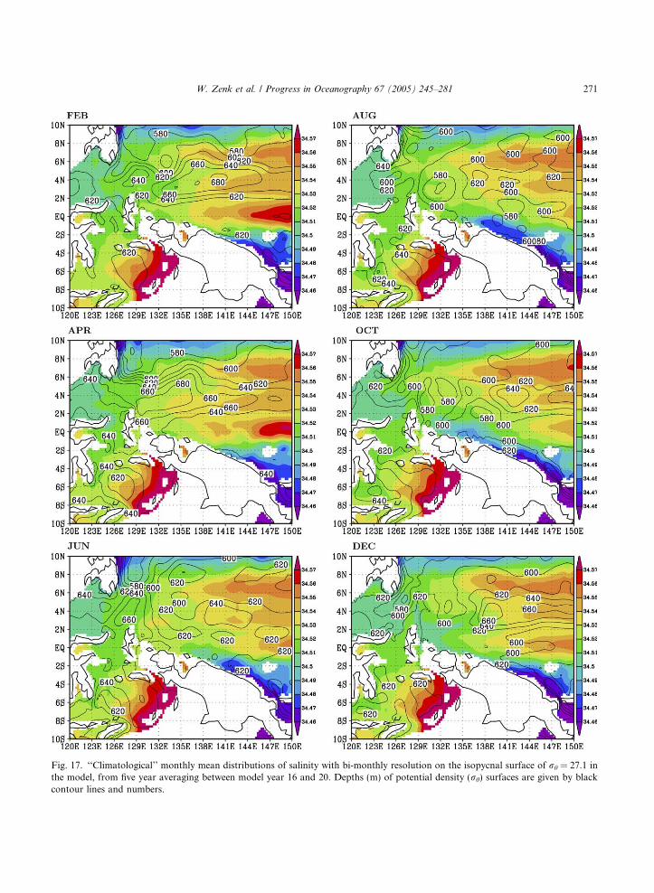
Fig. 17. ‘‘Climatological’’ monthly mean distributions of salinity with bi-monthly resolution on the isopycnal surface of rh = 27.1 inthe model, from five year averaging between model year 16 and 20. Depths (m) of potential density (rh) surfaces are given by blackcontour lines and numbers.
W. Zenk et al. / Progress in Oceanography 67 (2005) 245–281 271
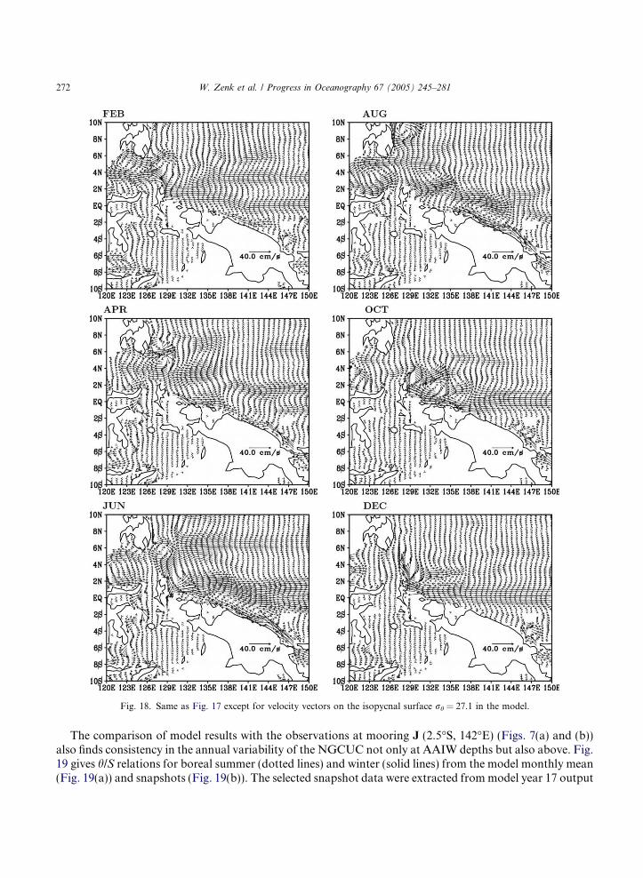
Fig. 18. Same as Fig. 17 except for velocity vectors on the isopycnal surface rh = 27.1 in the model.
272 W. Zenk et al. / Progress in Oceanography 67 (2005) 245–281
The comparison of model results with the observations at mooring J (2.5�S, 142�E) (Figs. 7(a) and (b))also finds consistency in the annual variability of the NGCUC not only at AAIW depths but also above. Fig.19 gives h/S relations for boreal summer (dotted lines) and winter (solid lines) from the model monthly mean(Fig. 19(a)) and snapshots (Fig. 19(b)). The selected snapshot data were extracted frommodel year 17 output

26.9
27.0
27.2
27.1
27.3
27.4
Salinity
Pot
entia
ltem
pera
ture
(deg
C)
Salinity
Pot
entia
ltem
pera
ture
(deg
C)
27.0
26.9
27.2
27.1
27.3
27.4
34.42 34.44 34.46 34.48 34.50 34.52 34.54 34.56 34.58
8.0
7.5
7.0
6.5
6.0
5.5
5.0
4.5
4.0
34.42 34.44 34.46 34.48 34.50 34.52 34.54 34.56 34.58
8.0
7.5
7.0
6.5
6.0
5.5
5.0
4.5
4.0
a
b
Fig. 19. Potential temperature–salinity relations in the AAIW Smin-layer from the modeled climatological monthly mean (a) andsnapshots at the calendar days near the observations (b) at the position of the current meter time series station J (2.5�S, 142.0�E).Contours indicate potential density rh.
W. Zenk et al. / Progress in Oceanography 67 (2005) 245–281 273
at the calendar day near the observation dates. The monthly mean data shows seasonal changes which arealso clearly seen in the observations (Fig. 6), although there are some differences such as too smooth adistribution in the model profiles, a slightly lower value of Smin-value, and lower density of the Smin-layer.
274 W. Zenk et al. / Progress in Oceanography 67 (2005) 245–281
The distribution from the model snapshots is more like the observed one because it has an intricate structurelike the observations. However, it is still too smooth. Some missing physics in the model such as interleavingprocesses might be responsible. Although the density of Smin in the model is nearly rh = 27.1, slightly lowerthan in the observations, it agrees with observations in that the seasonal variation is high not only in theSmin-layer but also between rh = 27.1 and 27.3. Thus the model reproduces significant seasonal variationsin a wide density range around the AAIW core as was recognized in the observations.
The NGCUC flow in the model at the AAIW level (Figs. 16 and 18) also shows clear annual vari-ations, with northwestward currents in boreal spring and summer (April–September) and southeastwardcurrents in boreal fall and winter (October–March). This is also apparent in the time series of zonalvelocity at the mooring site J (Fig. 7(b)) which were extracted from the model hindcast experimentto compare with the observed data (Fig. 7(a)). The model results are shown at the model grid levelsnearest the observed depths and for the same period as the observations. When comparing the modelvelocity at 874 m with the observational data at 850 m, we find that the model captures the strongwestward current in September and October 1998, displays a weaker current from December 1998through February 1999, and has relatively strong currents again from April through July 1999.Short-term variability is not well reproduced because the model output was sampled every 5 days incontrast to the daily observational data. The comparison at shallower depths (500 and 700 m) also findssimilar seasonal variations in the observations.
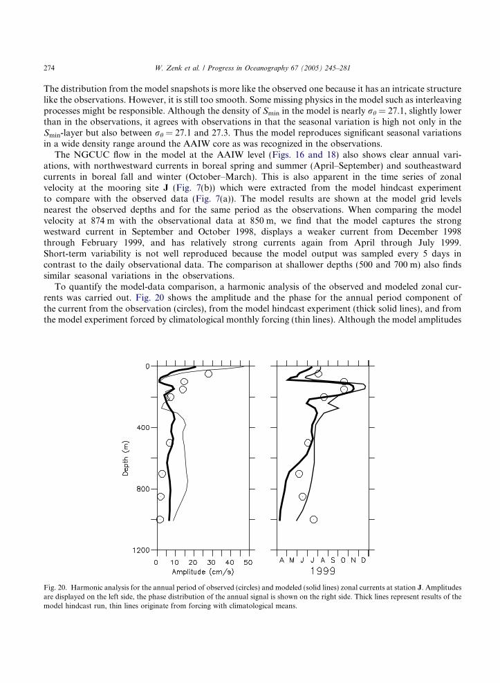
To quantify the model-data comparison, a harmonic analysis of the observed and modeled zonal cur-rents was carried out. Fig. 20 shows the amplitude and the phase for the annual period component ofthe current from the observation (circles), from the model hindcast experiment (thick solid lines), and fromthe model experiment forced by climatological monthly forcing (thin lines). Although the model amplitudes
Fig. 20. Harmonic analysis for the annual period of observed (circles) and modeled (solid lines) zonal currents at station J. Amplitudesare displayed on the left side, the phase distribution of the annual signal is shown on the right side. Thick lines represent results of themodel hindcast run, thin lines originate from forcing with climatological means.
W. Zenk et al. / Progress in Oceanography 67 (2005) 245–281 275
are slightly larger below 500 m and smaller in surface layers than those of the observations, the order of themagnitude of the current is well simulated in the hindcast experiment. The model also reproduces the ob-served characteristics in which the phase shows significant time lag between 100 and 150 m depth and sharpdifference below and above the subsurface layer. It is noted that both model and observations indicate anupward propagation of phase between 200 and 700 m. The westward current has its maximum early in Juneat 700 m, early in July at 500 m, and in mid-August at 200 m. The upward propagation might be indicativeof annual period equatorial Rossby waves (Kessler & McCreary, 1993). The model also suggests that theobserved upward phase propagation between 200 and 700 m represents a robust structure, although thereare uncertainties below 700 m.
The difference of the model amplitude and phase between the hindcast and climatological forcing exper-iments is caused by year to year variation of the currents. The good agreement between the observationsand the model hindcast suggests that the climatological mean amplitude between 400 and 800 m is largerthan that in the observational period by about 10 cm s�1.
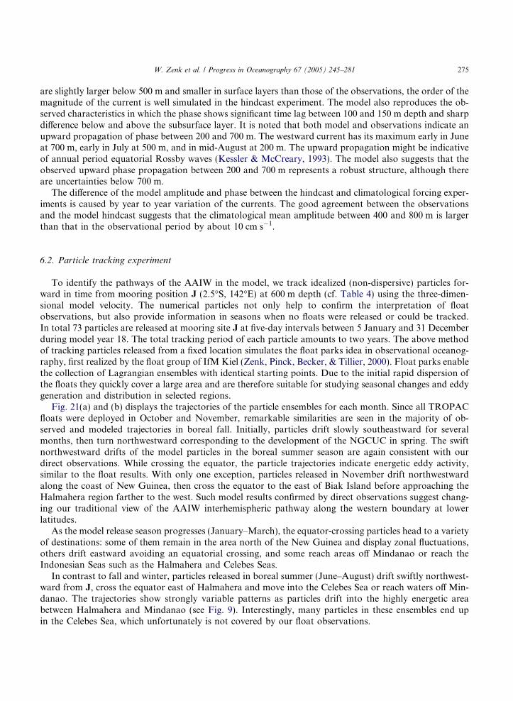
6.2. Particle tracking experiment
To identify the pathways of the AAIW in the model, we track idealized (non-dispersive) particles for-ward in time from mooring position J (2.5�S, 142�E) at 600 m depth (cf. Table 4) using the three-dimen-sional model velocity. The numerical particles not only help to confirm the interpretation of floatobservations, but also provide information in seasons when no floats were released or could be tracked.In total 73 particles are released at mooring site J at five-day intervals between 5 January and 31 Decemberduring model year 18. The total tracking period of each particle amounts to two years. The above methodof tracking particles released from a fixed location simulates the float parks idea in observational oceanog-raphy, first realized by the float group of IfM Kiel (Zenk, Pinck, Becker, & Tillier, 2000). Float parks enablethe collection of Lagrangian ensembles with identical starting points. Due to the initial rapid dispersion ofthe floats they quickly cover a large area and are therefore suitable for studying seasonal changes and eddygeneration and distribution in selected regions.
Fig. 21(a) and (b) displays the trajectories of the particle ensembles for each month. Since all TROPACfloats were deployed in October and November, remarkable similarities are seen in the majority of ob-served and modeled trajectories in boreal fall. Initially, particles drift slowly southeastward for severalmonths, then turn northwestward corresponding to the development of the NGCUC in spring. The swiftnorthwestward drifts of the model particles in the boreal summer season are again consistent with ourdirect observations. While crossing the equator, the particle trajectories indicate energetic eddy activity,similar to the float results. With only one exception, particles released in November drift northwestwardalong the coast of New Guinea, then cross the equator to the east of Biak Island before approaching theHalmahera region farther to the west. Such model results confirmed by direct observations suggest chang-ing our traditional view of the AAIW interhemispheric pathway along the western boundary at lowerlatitudes.
As the model release season progresses (January–March), the equator-crossing particles head to a varietyof destinations: some of them remain in the area north of the New Guinea and display zonal fluctuations,others drift eastward avoiding an equatorial crossing, and some reach areas off Mindanao or reach theIndonesian Seas such as the Halmahera and Celebes Seas.
In contrast to fall and winter, particles released in boreal summer (June–August) drift swiftly northwest-ward from J, cross the equator east of Halmahera and move into the Celebes Sea or reach waters off Min-danao. The trajectories show strongly variable patterns as particles drift into the highly energetic areabetween Halmahera and Mindanao (see Fig. 9). Interestingly, many particles in these ensembles end upin the Celebes Sea, which unfortunately is not covered by our float observations.
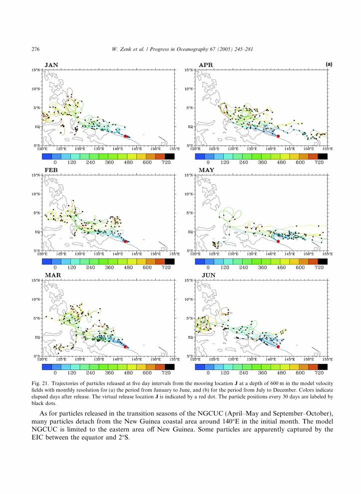
Fig. 21. Trajectories of particles released at five day intervals from the mooring location J at a depth of 600 m in the model velocityfields with monthly resolution for (a) the period from January to June, and (b) for the period from July to December. Colors indicateelapsed days after release. The virtual release location J is indicated by a red dot. The particle positions every 30 days are labeled byblack dots.
276 W. Zenk et al. / Progress in Oceanography 67 (2005) 245–281
As for particles released in the transition seasons of the NGCUC (April–May and September–October),many particles detach from the New Guinea coastal area around 140�E in the initial month. The modelNGCUC is limited to the eastern area off New Guinea. Some particles are apparently captured by theEIC between the equator and 2�S.
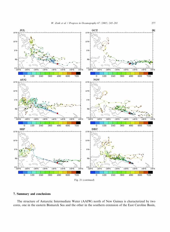
Fig. 21 (continued)
W. Zenk et al. / Progress in Oceanography 67 (2005) 245–281 277
7. Summary and conclusions
The structure of Antarctic Intermediate Water (AAIW) north of New Guinea is characterized by twocores, one in the eastern Bismarck Sea and the other in the southern extension of the East Caroline Basin,
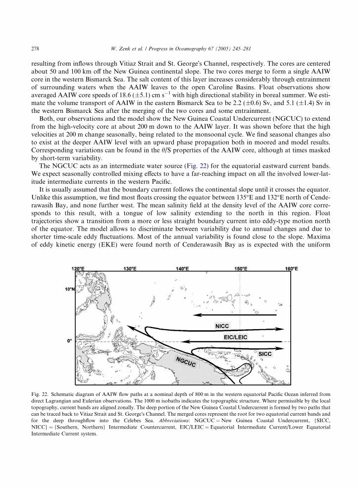
278 W. Zenk et al. / Progress in Oceanography 67 (2005) 245–281
resulting from inflows through Vitiaz Strait and St. George�s Channel, respectively. The cores are centeredabout 50 and 100 km off the New Guinea continental slope. The two cores merge to form a single AAIWcore in the western Bismarck Sea. The salt content of this layer increases considerably through entrainmentof surrounding waters when the AAIW leaves to the open Caroline Basins. Float observations showaveraged AAIW core speeds of 18.6 (±5.1) cm s�1 with high directional stability in boreal summer. We esti-mate the volume transport of AAIW in the eastern Bismarck Sea to be 2.2 (±0.6) Sv, and 5.1 (±1.4) Sv inthe western Bismarck Sea after the merging of the two cores and some entrainment.
Both, our observations and the model show the New Guinea Coastal Undercurrent (NGCUC) to extendfrom the high-velocity core at about 200 m down to the AAIW layer. It was shown before that the highvelocities at 200 m change seasonally, being related to the monsoonal cycle. We find seasonal changes alsoto exist at the deeper AAIW level with an upward phase propagation both in moored and model results.Corresponding variations can be found in the h/S properties of the AAIW core, although at times maskedby short-term variability.
The NGCUC acts as an intermediate water source (Fig. 22) for the equatorial eastward current bands.We expect seasonally controlled mixing effects to have a far-reaching impact on all the involved lower-lat-itude intermediate currents in the western Pacific.
It is usually assumed that the boundary current follows the continental slope until it crosses the equator.Unlike this assumption, we find most floats crossing the equator between 135�E and 132�E north of Cende-rawasih Bay, and none further west. The mean salinity field at the density level of the AAIW core corre-sponds to this result, with a tongue of low salinity extending to the north in this region. Floattrajectories show a transition from a more or less straight boundary current into eddy-type motion northof the equator. The model allows to discriminate between variability due to annual changes and due toshorter time-scale eddy fluctuations. Most of the annual variability is found close to the slope. Maximaof eddy kinetic energy (EKE) were found north of Cenderawasih Bay as is expected with the uniform
Fig. 22. Schematic diagram of AAIW flow paths at a nominal depth of 800 m in the western equatorial Pacific Ocean inferred fromdirect Lagrangian and Eulerian observations. The 1000 m isobaths indicates the topographic structure. Where permissible by the localtopography, current bands are aligned zonally. The deep portion of the New Guinea Coastal Undercurrent is formed by two paths thatcan be traced back to Vitiaz Strait and St. George�s Channel. The merged cores represent the root for two equatorial current bands andfor the deep throughflow into the Celebes Sea. Abbreviations: NGCUC = New Guinea Coastal Undercurrent, {SICC,NICC} = {Southern, Northern} Intermediate Countercurrent, EIC/LEIC = Equatorial Intermediate Current/Lower EquatorialIntermediate Current system.
W. Zenk et al. / Progress in Oceanography 67 (2005) 245–281 279
boundary current changing into eddy-type motion. A similar EKE pattern was found in the results from thecirculation model.
With respect to the eddy activity it is worth noting that none of the floats within the AAIW layer, neitherin-situ nor modeled, made their way to the north of 12�N. In particular, none of these floats connected theequatorial region with the Mindanao Undercurrent, thus supporting Wijffels� et al. (1998) hypothesis thatthe high oxygen signal along the western boundary in the North Pacific results from eddy fluxes rather thanbeing a signature of a mean undercurrent.
According to the float observations, the AAIW-derived water finally is embedded in the zonal equatorialflows of the Southern and Northern Intermediate Countercurrents (SICC, NICC) within about ±2� off theequator. We find an amazing consistency of different observational and model average zonal currents.
Although the results from the numerical experiments appear to be largely consistent with the observa-tions, the AAIW core depths are somewhat shallower in the model than in the observations. Supplementingthe limited observations in time and space, the model indicates that the westward velocity in the observa-tion period was significantly larger (by about 10 cm s�1) than the climatological mean due to interannualvariability in wind forcing.
The particle tracking model experiment exhibits considerable seasonal changes in the character of theflow. For selected seasons the observed float tracks can be used for the validation of model tracks. Althoughreasonable agreement provides confidence in tentatively accepting the model results for the full year, variouspatterns of tracks and destinations differ in detail and suggest the need for further observations.
Acknowledgements
The authors are indebted to R. Onken for his help in the planning of the TROPAC experiment, to thestaff of the earlier Department of Marine Physics of the Institut fur Meereskunde in Kiel, Germany, formany contributions to observations and data processing, and to the captains and crews of the research ves-sels SONNE, KAIYO and HAKUHO MARU for most helpful advice and cooperation. With pleasure weacknowledge the diligent work of O. Boebel and C. Schmid who were in charge of ballasting and fine-tuningthe RAFOS floats. We benefited from discussions with K. Taira and M. Kawabe and from their assistancein the German–Japanese mooring work. The second author (G.S.) performed part of the data analysis dur-ing a stay at the International Pacific Research Center (IPRC) at the School of Ocean and Earth Scienceand Technology (SOEST) of the University of Hawaii, USA. The discussions with members of the IPRCand other colleagues at SOEST were much appreciated. The TROPAC project was funded by the Ministryof Science and Technology, Germany (BMFT 03G0113A, 03F0176A, 03F0157A) and the Ministry of Edu-cation, Culture, Sports, Science and Technology, Japan (MEXT). JAMSTEC observation cruises north ofNew Guinea using the research vessel KAIYO were conducted under the TOCS project funded by theMEXT, and in a joint project with the Ocean Research Institute of the University of Tokyo. Special thanksgo to technicians of the Marine Work Japan Co. Ltd. and Nihon Marine Enterprise Co. Ltd., and otherparticipants. Finally, the help of J.M. Toole during the revision phase of the manuscript is appreciated.
References
Bingham, F. M., & Lukas, R. (1995). The distribution of intermediate water in the western equatorial Pacific during January–February1986. Deep-Sea Research, 42, 1545–1573.
Bryden, H. L., & Imawaki, S. (2001). Large-scale ocean transports. In G. Siedler, J. Church, & J. Gould (Eds.), Ocean circulation and
climate (pp. 455–474). London: Academic Press.Butt, J., & Lindstrom, E. (1994). Currents off the east coast of New Ireland, Papua New Guinea, and their relevance to regional
undercurrents in the Western Equatorial Pacific Ocean. Journal of Geophysical Research, 99, 12503–12514.

280 W. Zenk et al. / Progress in Oceanography 67 (2005) 245–281
Cresswell, G. R. (2000). Coastal currents of northern Papua New Guinea, and the Sepik River outflow. Marine and Freshwater
Research, 51(6), 553–564.Delcroix, T., & Henin, C. (1988). Observations of the Equatorial Intermediate Current in the western Pacific Ocean (165�E). Journal of
Physical Oceanography, 18, 363–366.Davis, R. E. (1998). Preliminary results from directly measuring mid-depth circulation in the tropical and South Pacific. Journal of
Geophysical Research, 103, 24619–24639.England, M. H. (1992). On the formation of Antarctic Intermediate Bottom Water in ocean general circulation models. Journal of
Physical Oceanography, 22, 918–926.Fine, R. A., Lukas, R., Bingham, F. M., Warner, M. J., & Gammon, R. H. (1994). The western equatorial pacific: a water mass
crossroads. Journal of Geophysical Research, 99(C12), 25063–25080.Firing, E., Wijffels, S. E., & Hacker, P. (1998). Equatorial subthermocline currents across the Pacific. Journal of Geophysical Research,
103(C10), 21413–21423.Gouriou, Y., & Toole, J. (1993). Mean circulation of the upper layers of the western equatorial Pacific Ocean. Journal of Geophysical
Research, 98(C12), 22495–22520.Hanawa, K., & Talley, L. D. (2001). Mode waters. In G. Siedler, J. Church, & J. Gould (Eds.), Ocean circulation and climate
(pp. 373–386). London: Academic Press.Hellerman, S., & Rosenstein, M. (1983). Normal monthly wind stress over the world ocean with error estimates. Journal of Physical
Oceanography, 13, 1093–1104.Hiller, W. & Kase, R. H. (1983). Objective analysis of hydrographic data sets from mesoscale surveys. Berichte Institut fur
Meereskunde Kiel, 116, 78 pp (unpublished manuscript).Huang, R. X., & Russell, S. (1994). Ventilation of the subtropical North Pacific. Journal of Physical Oceanography, 24, 2589–2605.Imawaki, S., Zenk, W., Wijffels, S., Roemmich, D., & Kawabe, M. (2001). Oceanic boundary currents. In C. J. Koblinsky & N. R.
Smith (Eds.), Observing the Ocean in the 21st Century (pp. 285–305). .Ioualalen, M., Siedler, G., Zenk, W., Henin, C., & Picaut, J. (2000). The equatorial West Pacific fresh pool at the end of the La Nina
event in October/November 1996. Geophysical Research Letters, 9, 1243–1246.Ishida, A., Kashino, Y., Mitsudera, H., Yoshioka, N., & Kadokura, T. (1998). Preliminary results of a global high-resolution GCM
experiment. Journal of the Faculty of Science, Hokkaido University, Series VII (Geophysics), 11(2), 441–460.Kashino, Y., Aoyama, M., Kawano, T., Hendiarti, N., Anantasena, Y., Muneyama, K., et al. (1996). The water masses between
Mindanao and New Guinea. Journal of Geophysical Research, 101(C5), 12 391–12 400.Kashino, Y., Hase, H., Ando, K., Yoneyama, K., Takatsuki, Y., Kuroda, Y., & Mizuno, K. (2001). TOCS Data Report 2: 1995–2000.
TOCS No.4, Ocean Observation and Research Department, Japan Marine Science and Technology Center 2-15 NatsushimaYokosuka 372 pp (unpublished manuscript).
Kashino, Y., Watanabe, H., Herunadi, B., Aoyama, M., & Hartoyo, D. (1999). Current variability at the Pacific entrance of theIndonesian Throughflow. Journal of Geophysical Research, 104(C5), 11021–11035.
Kessler, W. S., & McCreary, J. P. (1993). The annual wind-driven Rossby wave in the subthermocline equatorial Pacific. Journal ofPhysical Oceanography, 23, 1192–1207.
Konig, H. & Zenk, W. (1992). Principles of RAFOS technology at the Institut fur Meereskunde Kiel. Berichte Institut fur Meereskunde
Kiel, 222, 99 pp (unpublished manuscript).Levitus, S. (1982). Climatological atlas of the world oceans. NOAA Professional Paper 13 (173 pp). Princeton, NJ.Lindstrom, E., Butt, J., Lukas, R., & Godfrey, S. (1990). The flow through Vitiaz Strait and St. George�s Channel. In L. J. Pratt (Ed.),
The physical oceanography of sea straits (pp. 171–189). Dordtrecht: Kluwer Academic.Lindstrom, E., Lukas, R., Fine, R., Firing, E., Godfrey, S., Meyers, G., et al. (1987). The Western Equatorial Pacific Ocean
Circulation Study. Nature, 330, 533–537.Luyten, J. R., Pedlosky, J., & Stommel, H. (1983). The ventilated thermocline. Journal of Physical Oceanography, 13, 292–309.McCartney, M. S. (1977). Subantarctic mode water. In M. Angel (Ed.), A voyage of Discovery, George Deacon 70th anniversary volume
(pp. 103–119). Oxford: Pergamon Press.McCreary, J. P., & Lu, P. (2001). Influence of the Indonesian Throughflow on the Circulation of Pacific Intermediate Water. Journal of
Physical Oceanography, 31, 932–942.Pacanowski, R. C. (1995). MOM2 Documentation, User�s Guide and Reference Manual. Technical Report 3, GFDL Ocean Group
Technical Report 3 (232 pp.). Princeton, NJ (unpublished manuscript).Pacanowski, R. C., & Philander, S. G. H. (1981). Parameterization of vertical mixing in numerical models of tropical oceans. Journal of
Physical Oceanography, 11, 1443–1451.Reid, J. L. (1965). Intermediate waters of the Pacific Ocean. Johns Hopkins Oceanographic Studies, 2, 85 pp.Reynolds, R. W., & Smith, T. M. (1994). Improved global sea surface temperature analysis using optimum interpolation. Journal of
Climate, 7, 929–948.Rossby, H. T., Dorson, D., & Fontain, J. (1986). The RAFOS system. Journal of Atmospheric and Oceanographic Technology, 3,
672–679.

W. Zenk et al. / Progress in Oceanography 67 (2005) 245–281 281
Saunders, P. M., Coward, A. C., & de Cuevas, B. A. (1999). Circulation of the Pacific Ocean seen in a global ocean model: Oceancirculation and climate advanced modelling project (OCCAM). Journal of Geophysical Research, 104(C8), 18281–18299.
Schmid, C., Siedler, G., & Zenk, W. (2000). Dynamics of Intermediate Water Circulation in the Subtropical South Atlantic. Journal ofPhysical Oceanography, 30, 3191–3211.
Siedler, G., Holfort, J., Zenk, W., Muller, T. J., & Csernok, T. (2004). Deep water flow pattern in the Mariana and Caroline Basins.Journal of Physical Oceanography, 34, 566–581.
Siedler, G. & Zenk, W. (1997). Untersuchungen zu den tiefen Wassermassen und planktologische Beobachtungen im tropischenWestpazifik wahrend der SONNE-Fahrt 113 (TROPAC). Berichte Institut fur Meereskunde Kiel, 288, 129 pp (unpublishedmanuscript).
Sloyan, B. M., & Rintoul, S. R. (2001). Circulation, renewal and modification of Antarctic mode and intermediate water. Journal ofPhysical Oceanography, 31, 1005–1030.
Smith, W. H. F., & Sandwell, D. T. (1997). Global Sea Floor Topography from Satellite Altimetry and Ship Depth Soundings. Science,277, 1956–1962.
Sprintall, J., Wijffels, S., Chereskin, T., & Bray, N. (2002). The JADE and WOCE I10/IR6 throughflow sections in the southeasternIndian Ocean, Part 2: Velocity and transports. Deep-Sea Research II, 49(7–8), 1363–1389.
Talley, L. D. (1993). Distribution and formation of North Pacific Intermediate Water. Journal of Physical Oceanography, 23, 517–537.Tomczak, M., & Godfrey, J. (1994). Regional oceanography: An introduction. London: Pergamon Press, 422 pp.Tsuchiya, M. (1968). Upper waters of the intertropical Pacific Ocean. Johns Hopkins Oceanographic Studies, 4, 1–50.Tsuchiya, M. (1975). Subsurface countercurrents in the eastern equatorial Pacific Ocean. Journal of Marine Research, 33(suppl.),
145–175.Tsuchiya, M. (1991). Flow path of the Antarctic Intermediate Water in the western equatorial South Pacific Ocean. Deep-Sea
Research, 38(suppl.), S273–S279.Tsuchiya, M., Lukas, R., Fine, R. A., Firing, E., & Lindstrom, E. (1989). Source waters of the Pacific Equatorial Undercurrent.
Progress in Oceanography, 23, 101–147.Ueki, I., Kashino, Y., & Kuroda, Y. (2003). Observation of current variation off New Guinea coast including the 1997–98 El Nino
period and its relationship with Sverdrup transport. Journal of Geophysical Research, 108, 3243. doi:10.1029/2002JC001611.Wijffels, S. E., Hall, M. M., Joyce, T., Torres, D. J., Hacker, P., & Firing, E. (1998). Multiple deep gyres of the western North Pacific: a
WOCE section along 149E. Journal of Geophysical Research, 103, 12985–13009.Wyrtki, K. (1961). Physical Oceanography of the Southeast Asian Waters. NAGA Report 2, The University of California, Scripps
Institution of Oceanography, La Jolla, California 195 pp.Wyrtki, K., & Kilonsky, B. (1984). Mean water and current structures during the Hawaii-to-Tahiti shuttle experiment. Journal of
Physical Oceanography, 14, 242–254.Zenk, W., Pinck, A., Becker, S., & Tillier, P. (2000). The float park: A new tool for a cost-effective collection of Lagrangian time-series
with dual release RAFOS floats. Journal of Atmospheric and Oceanic Technology, 17, 1439–1443.