Particle Identification with MPD-TPCtracks

MexNICA Collaboration Winter Meeting

Julio César Maldonado González

December 16th, 2020

Facultad de Informática Culiacán - Universidad Autónoma de Sinaloa

Table of contents

1. Introduction

2. Reconstruction

3. Bayesian method

4. Data Science Techniques

5. Further work

Introduction

Introduction

• Particles are accelerated and collided at high energies.• We can only see the information stored in the detectors translated

into the form of tracks of the trajectories of the particles. [1]

Introduction

This project will participate in the particle identification analysis used inthe simulation and generation of events to study physics in heavy ioncollisions for the Multi-Purpose Detector (MPD) experiment of theNuclotron Ion Collider fAcility (NICA) at the Joint Institute for NuclearResearch (JINR) in Dubna, Russia.

Figure 1: MPD sub-detectors at NICA. [3]

Introduction

• In the experimental high energies physics, it is essential to identifythe type of particle that occurs in the Particle Identification (PID)experiment.

• These identification techniques depend on the properties orobservables that are obtained from the experiment. [2]

• From reconstruction on the tracks of the particles, you can get themomentum, energy loss, and other features of the particles as theypass through the TPC detector.

• MPD tracks features could be used as input data for machinelearning techniques like GLMs models.

• Statistical methods (Bayesian approach) results could be comparewith results obtained by machine learning.

Reconstruction

Reconstruction

• The event reconstruction consists in finding particles tracks usingthe Kalman filter technique. [3]

• The physics analysis consists in finding the PID from observablesignals from detectors through reconstruction data.

Reconstruction

A brief example of a MPDROOT macro to read reconstruction files:

Data for simulation and reconstruction

• Detector: MPD (TPC)

• Input file: reconstruction.root file (DST)

• Event generator: UrQMD

• Bi-Bi a 11 GeV (MB)

• Number of events: 10k

• Macro base: CompareSpectra.C, anaDST.C

Cuts suggested in the TPC documentation [7]

• Eta cut (η< 1.2)

• PT cut (1.0>PT > 0.1)

• Primary and secondary particles (MotherID ≤ 0, MotherID > 0 )

Bayesian method

Bayesian method

The probability of a particle i , if a signal s is observed,

ω(i |s) =r(s |i)Ci

∑

k r(s |k)Ck

• r(s |i) Conditional probability density function of the signal observeds of a detector, if a particle i(e,µ,π,K ,p, ...)is detected. It reflectsproperties of the detector.

• Ci is the probability of finding a particle type in the detector(frequency). It does not depend on the detector.

Probability density functions

Using the TPC, s is the signal dE/dx assigned to each track from thereconstruction.

2000 2500 3000 3500 4000dE/dx, ADC Counts

0

200

400

600

800

1000

1200

1400

1600

1800

2000

dN/(

dE/d

x)

dE/dx pion

dE/dx TPC

dE/dx pion

2000 2500 3000 3500 4000dE/dx, ADC Counts

0

50

100

150

200

250

300

350

400

dN/(

dE/d

x)

dE/dx pion

dE/dx TPC

dE/dx pion

Figure 2: dE/dx from TPC for 10k events taking the momentum range of0.28 to 0.32 GeV/c in [6] for primary and secondary particles.

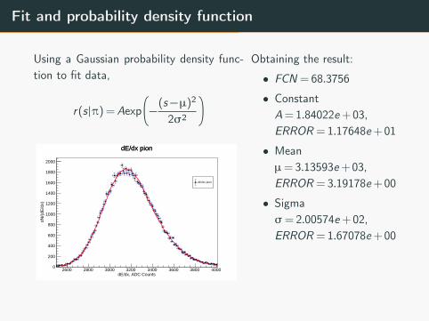
Fit and probability density function

Using a Gaussian probability density func-tion to fit data,

r(s |π) =Aexp�

−(s −µ)2

2σ2

�

2600 2800 3000 3200 3400 3600 3800 4000dE/dx, ADC Counts

0

200

400

600

800

1000

1200

1400

1600

1800

2000

dN/(

dE/d

x)

dE/dx pion

dE/dx pion

dE/dx pion

Obtaining the result:

• FCN = 68.3756

• ConstantA= 1.84022e+03,ERROR = 1.17648e+01

• Meanµ= 3.13593e+03,ERROR = 3.19178e+00

• Sigmaσ= 2.00574e+02,ERROR = 1.67078e+00

Probabilities a priori Ci

The probabilities Ci can be estimated with Time-of-Flight measurements,

m=p

βγ= p

√

√c2t2

l2−1

0 0.2 0.4 0.6 0.8 1 1.2 1.4 1.6 1.8 22)2, (GeV/c2M

0

500

1000

1500

2000

2500

3000

3500

2dN

/dM

M2 TOF

M^2 TOF

M2 TOF

Figure 3: M2 TOF for 10k events for primary particles.

Probabilities a priori Ci

Taking each peak in an histogram, we have Cp = 741 and Cπ= 175

0.6 0.7 0.8 0.9 1 1.1 1.22)2, (GeV/c2M

0

100

200

300

400

500

600

700

8002dN

/dM

M2 proton

M^2

M2 proton

0.2 0.21 0.22 0.23 0.24 0.25 0.26 0.27 0.282)2, (GeV/c2M

0

20

40

60

80

100

120

140

160

180

2dN

/dM

M2 pion

M^2 TOF

M2 pion

Data Science Techniques

Classification models

In high-energy physics, statistical techniques are traditionally used todetermine a mathematical function f (x).

In machine learning we have the approximate function f (x ,w) from a testdata set, {x ,y}, with x the feature vector, and y the relation betweenthose features.

We seek to obtain the model parameters w.

Generalized Linear Model (GLM)

In a generalized linear model, the response yi ,

yi = β0+β1x1i + ...+βpxpi + εi

with variables xj and an error term εi .

GLMs can be applied with R using the function glm,

y ∼ x1+ x2

• y is the response (type of particle: "proton particule" or "pionparticles").

• x1,x2 are numeric feature vectors (momentum "P" and energydeposition "dEdx".)

Generalized Linear Model (GLM)

Generalized Linear Model (GLM)

We use a data set for training (defining parameters model) with twoclasses: pions (211) and protons (2212).

P dEdx PDGID0.377411 2782.666 2110.633236 2715.193 2110.404283 2710.947 2110.749252 3044.496 2110.423279 13775.852 22120.353684 2907.477 211

Generalized Linear Model (GLM)

Coefficients:

Estimate Std. Error(Intercept) -7.51945 12.06997

dEdx 0.00377 0.00365P 8.06809 9.61674

The discriminant function can be write as follow,

y =−7.51954+(0.00377)dEdx+(8.06809)P

A test data element is defined as followed, obtaining a probability from 0to 1 for both classes (protons (0) and pions(1)),

newdata = data.frame(P = 0.377411, dEdx = 2782.666)predict(model, newdata, type="response")

Further work

Further work

• Implement r(s |i) probability density functions and Ci obtain fromhistograms to calculate bayesian conditional probability ω(i |s).

• Compare with GLM model results implementing in R for a binomialclass data set.

• Expand GLM model to a more complex model made by several GLMindividual models.

• Using larger data set made from larger numbers of events forprotons, pions, kaons and electrons.

References

[1] C. Lippmann (2011) Particle identification. Nucl. Instrum. Meth.,vol. A666, pp. 148–172, 2012.DOI:10.1016/j.nima.2011.03.009.

[2] E. Garutti, Particle Identification (PID). Distinguishing particle typeshttp://www.desy.de/ garutti/LECTURES/ParticleDetectorSS12/

[3] O. Rogachevsky (2020) Purposes of the MpdRoot framework –MPD EXPERIMENThttp://mpd.jinr.ru/mpdroot-start-guide/

[4] Dryablov, D., Gudima, K., Kapishin, M., Litvinenko, E.,Musulmanbekov, G., Zheger, V. (2013). Event CentralityDetermination and Reaction Plane Reconstruction at MPD.

[5] Kryshen, E. Ivanishchev, D Kotov, Dmitry Malaev, M Riabov, VRyabov, Yu. (2019). Study of neutral meson production withphoton conversions in the MPD experiment at NICA. Journal ofPhysics: Conference Series. 1400. 055055.10.1088/1742-6596/1400/5/055055.

[6] Mudrokh, Alexander. (2019). Prospects for the study of

event-by-event fluctuations at MPD/NICA project. EPJ Web ofConferences. 204. 07014. 10.1051/epjconf/201920407014.

[7] A. Averyanov et al. (2017). TPC status for MPD experiment ofNICA project. JINST 12 C06047