
Part II of Fundamentals of Source and Video Coding - Stanford ...
77
2 Acquisition, Representation, Display, and Perception of Image and Video Signals In digital video communication, we typically capture a natural scene by a camera, transmit or store data representing the scene, and finally reproduce the captured scene on a display. The camera converts the light emitted or reflected from objects in a three-dimensional scene into arrays of discrete-amplitude samples. In the display device, the arrays of discrete-amplitude samples are converted into light that is emitted from the display and perceived by human beings. The primary task of video coding is to represent the sample arrays generated by the camera and used by the display device with a small number of bits, suitable for transmission or storage. Since the achievable compression for an exact representation of the sample arrays recorded by a camera is not sufficient for most applications, the sample arrays are modified in a way that they can be represented with a given maximum number of bits or bits per time unit. Ideally, the degradation of the perceived image quality due to the modifications of the sample arrays should be as small as possible. Hence, even though video coding eventually deals with mapping arrays of discrete-amplitude samples into a bitstream, the quality of the displayed video is largely influenced by the way we acquire, represent, display, and perceive visual information. 7
-
Upload
khangminh22 -
Category
Documents
-
view
2 -
download
0
Transcript of Part II of Fundamentals of Source and Video Coding - Stanford ...
2Acquisition, Representation, Display, andPerception of Image and Video Signals
In digital video communication, we typically capture a natural sceneby a camera, transmit or store data representing the scene, and finallyreproduce the captured scene on a display. The camera converts thelight emitted or reflected from objects in a three-dimensional sceneinto arrays of discrete-amplitude samples. In the display device, thearrays of discrete-amplitude samples are converted into light that isemitted from the display and perceived by human beings. The primarytask of video coding is to represent the sample arrays generated by thecamera and used by the display device with a small number of bits,suitable for transmission or storage. Since the achievable compressionfor an exact representation of the sample arrays recorded by a camerais not sufficient for most applications, the sample arrays are modifiedin a way that they can be represented with a given maximum numberof bits or bits per time unit. Ideally, the degradation of the perceivedimage quality due to the modifications of the sample arrays should beas small as possible. Hence, even though video coding eventually dealswith mapping arrays of discrete-amplitude samples into a bitstream,the quality of the displayed video is largely influenced by the way weacquire, represent, display, and perceive visual information.
7
8 Acquisition, Representation, Display, and Perception
Certain properties of human visual perception have in fact a largeimpact on the construction of cameras, the design of displays, andthe way visual information is represented as sample arrays. And eventhough today’s video coding standards have been mainly designed froma signal processing perspective, they provide features that can be usedfor exploiting some properties of human vision. A basic knowledge ofhuman vision, the design of camera and displays, and the used represen-tation formats is essential for understanding the interdependencies ofthe various components in a video communication system. For design-ing video coding algorithms, it is also important to know what impactchanges in the sample arrays, which are eventually coded, have on theperceived quality of images and video.
In the following section, we start with a brief review of basic prop-erties of image formation by lenses. Afterwards, we discuss certain as-pects of human vision and describe raw data formats that are usedfor representing visual information. Finally, an overview of the designof cameras and displays is given. For additional information on thesetopics, the reader is referred the comprehensive overview in [70].
2.1 Fundamentals of Image Formation
In digital cameras, a three-dimensional scene is projected onto an imagesensor, which measures physical quantities of the incident light andconverts them into arrays of samples. For obtaining an image of thereal world on the sensors surface, we require a device that projects allrays of light that are emitted or reflected from an object point and fallthrough the opening of the camera into a point in the image plane.The simplest of such devices is the pinhole by which basically all light,except a single pencil of rays, coming from a particular object pointis blocked from reaching the light-sensitive surface. Due to their badoptical resolution and extremely low light efficiency, pinhole optics arenot used in practice, but lenses are used instead. In the following, wereview some basic properties of image formation using lenses. For moredetailed treatments of the topic of optics, we recommend the classicreferences by Born and Wolf [6] and Hecht [33].
2.1. Fundamentals of Image Formation 9
2.1.1 Image Formation with Lenses
Lenses consist of transparent materials such as glass. They change thedirection of light rays falling through the lens due to refraction at theboundary between the lens material and the surrounding air. The shapeof a lens determines how the wavefronts of the light are deformed.Lenses that project all light rays originating from an object point intoa single image point have a hyperbolic shape at both sides [33]. This is,however, only valid for monochromatic light and a single object point;there are no lens shapes that form perfect images of objects. Since it iseasier and less expensive to manufacture lenses with spherical surfaces,most lenses used in practice are spherical lenses. Aspheric lenses are,however, often used for minimizing aberration in lens systems.
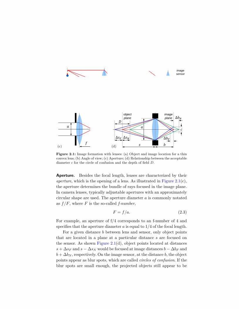
Thin Lenses. We restrict our considerations to paraxial approxima-tions (the angles between the light rays and the optical axis are verysmall) for thin lenses (the thickness is small compared to the radii ofcurvature). Under these assumptions, a lens projects an object in adistance s from the lens onto an image plane located at a distance b atthe other side of the lens, see Figure 2.1(a). The relationship betweenthe object distance s and the image distance b is given by
1s
+ 1b
= 1f, (2.1)
which is known as Gaussian lens formula (a derivation is, for example,given in [33]). The quantity f is called the focal length and representsthe distance from the lens plane, in which light rays that are parallelto the optical axis are focused into a single point.
For focusing objects at different locations, the distance b betweenlens and image sensor can be modified. Far objects (s→∞) are infocus if the distance b is approximately equal to the focal length f . Asillustrated in Figure 2.1(b), for a given image sensor, the focal length fof the lens determines the field of view. With d representing the width,height, or diagonal of the image sensor, the angle of view is given by
θ = 2 arctan(d
2 f
). (2.2)
10 Acquisition, Representation, Display, and Perception
𝑓 𝑓𝑠 𝑏
object
plane
image
plane
𝑏 ≈ 𝑓
𝑑
θ
image
sensor
(a) (b)
𝑓
𝑎
Δ𝑏𝐹
𝑎
𝑠 𝑏
object
plane
image
plane
𝑐
Δ𝑠𝑁Δ𝑠𝐹
Δ𝑏𝑁𝐷
(c) (d)
Figure 2.1: Image formation with lenses: (a) Object and image location for a thinconvex lens; (b) Angle of view; (c) Aperture; (d) Relationship between the acceptablediameter c for the circle of confusion and the depth of field D.
Aperture. Besides the focal length, lenses are characterized by theiraperture, which is the opening of a lens. As illustrated in Figure 2.1(c),the aperture determines the bundle of rays focused in the image plane.In camera lenses, typically adjustable apertures with an approximatelycircular shape are used. The aperture diameter a is commonly notatedas f/F , where F is the so-called f-number,
F = f/a. (2.3)
For example, an aperture of f/4 corresponds to an f-number of 4 andspecifies that the aperture diameter a is equal to 1/4 of the focal length.
For a given distance b between lens and sensor, only object pointsthat are located in a plane at a particular distance s are focused onthe sensor. As shown Figure 2.1(d), object points located at distancess+ ∆sF and s−∆sN would be focused at image distances b−∆bF andb+ ∆bN , respectively. On the image sensor, at the distance b, the objectpoints appear as blur spots, which are called circles of confusion. If theblur spots are small enough, the projected objects still appear to be
2.1. Fundamentals of Image Formation 11
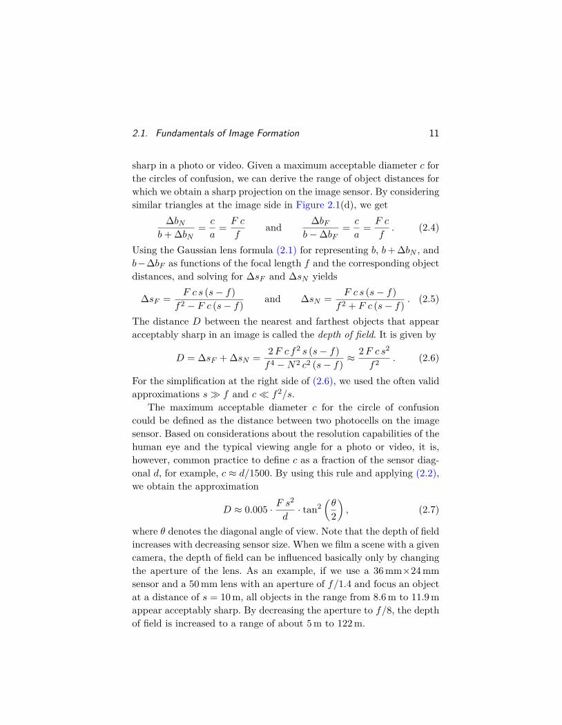
sharp in a photo or video. Given a maximum acceptable diameter c forthe circles of confusion, we can derive the range of object distances forwhich we obtain a sharp projection on the image sensor. By consideringsimilar triangles at the image side in Figure 2.1(d), we get
∆bNb+ ∆bN
= c
a= F c
fand ∆bF
b−∆bF= c
a= F c
f. (2.4)
Using the Gaussian lens formula (2.1) for representing b, b+ ∆bN , andb−∆bF as functions of the focal length f and the corresponding objectdistances, and solving for ∆sF and ∆sN yields
∆sF = F c s (s− f)f2 − F c (s− f) and ∆sN = F c s (s− f)
f2 + F c (s− f) . (2.5)
The distance D between the nearest and farthest objects that appearacceptably sharp in an image is called the depth of field. It is given by
D = ∆sF + ∆sN = 2F c f2 s (s− f)f4 −N2 c2 (s− f) ≈
2F c s2
f2 . (2.6)
For the simplification at the right side of (2.6), we used the often validapproximations s� f and c� f2/s.
The maximum acceptable diameter c for the circle of confusioncould be defined as the distance between two photocells on the imagesensor. Based on considerations about the resolution capabilities of thehuman eye and the typical viewing angle for a photo or video, it is,however, common practice to define c as a fraction of the sensor diag-onal d, for example, c ≈ d/1500. By using this rule and applying (2.2),we obtain the approximation
D ≈ 0.005 · F s2
d· tan2
(θ
2
), (2.7)
where θ denotes the diagonal angle of view. Note that the depth of fieldincreases with decreasing sensor size. When we film a scene with a givencamera, the depth of field can be influenced basically only by changingthe aperture of the lens. As an example, if we use a 36 mm×24mmsensor and a 50mm lens with an aperture of f/1.4 and focus an objectat a distance of s = 10m, all objects in the range from 8.6m to 11.9mappear acceptably sharp. By decreasing the aperture to f/8, the depthof field is increased to a range of about 5m to 122m.
12 Acquisition, Representation, Display, and Perception
𝑦
𝑍
𝑃 = (𝑋, 𝑌, 𝑍)
image
plane
object
point
𝑏 ≈ 𝑓
center of lens in point (0, 0, 0)𝑋
𝑌
𝑥
𝑝 = (𝑥, 𝑦)
lens
plane
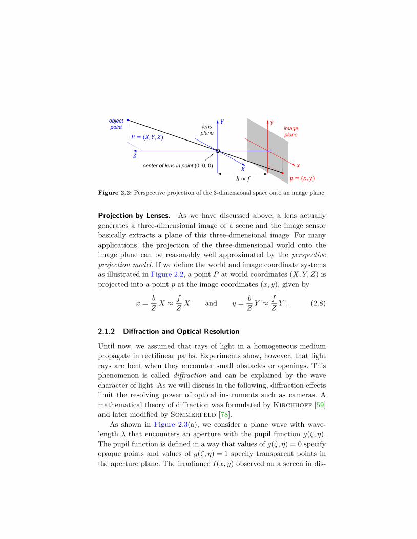
Figure 2.2: Perspective projection of the 3-dimensional space onto an image plane.
Projection by Lenses. As we have discussed above, a lens actuallygenerates a three-dimensional image of a scene and the image sensorbasically extracts a plane of this three-dimensional image. For manyapplications, the projection of the three-dimensional world onto theimage plane can be reasonably well approximated by the perspectiveprojection model. If we define the world and image coordinate systemsas illustrated in Figure 2.2, a point P at world coordinates (X,Y, Z) isprojected into a point p at the image coordinates (x, y), given by
x = b
ZX ≈ f
ZX and y = b
ZY ≈ f
ZY . (2.8)
2.1.2 Diffraction and Optical Resolution
Until now, we assumed that rays of light in a homogeneous mediumpropagate in rectilinear paths. Experiments show, however, that lightrays are bent when they encounter small obstacles or openings. Thisphenomenon is called diffraction and can be explained by the wavecharacter of light. As we will discuss in the following, diffraction effectslimit the resolving power of optical instruments such as cameras. Amathematical theory of diffraction was formulated by Kirchhoff [59]and later modified by Sommerfeld [78].
As shown in Figure 2.3(a), we consider a plane wave with wave-length λ that encounters an aperture with the pupil function g(ζ, η).The pupil function is defined in a way that values of g(ζ, η) = 0 specifyopaque points and values of g(ζ, η) = 1 specify transparent points inthe aperture plane. The irradiance I(x, y) observed on a screen in dis-

2.1. Fundamentals of Image Formation 13
wavelength 𝜆
𝑧
𝑥
𝑦𝜂
𝜁
aperture 𝑔(𝜁, 𝜂) screen
irradiance𝐼(𝑥, 𝑦)
𝑅
𝑓
sensor plane
(a) (b)
Figure 2.3: Diffraction in cameras: (a) Diffraction of a plane wave at an aperture;(b) Diffraction in cameras can be modeled using Fraunhofer diffraction.
tance z depends on the spatial position (x, y). For z � a2/λ, with a be-ing the largest dimension of the aperture, the phase differences betweenthe individual contributions that are superposed on the screen onlydepend on the viewing angles given by sinφ = x/R and sin θ = y/R,with R =
√x2 + y2 + z2. This far-field approximation is referred to as
Fraunhofer diffraction. Since a lens placed behind an aperture focusesparallel light rays in a point, as illustrated in Figure 2.3(b), diffractionobserved in cameras can be modeled using Fraunhofer diffraction. Theobserved irradiance pattern [33] is given by
I(x, y) = C ·∣∣∣∣G( x
λR,y
λR
)∣∣∣∣2 , (2.9)
where C is a constant and G(u, v) represents the two-dimensionalFourier transform of the pupil function g(ζ, η). For a camera with acircular aperture, the diffraction pattern on the sensor [33] in distancez ≈ f is given by
I(r) = I0 ·(2 J1(β r)
β r
)2with β = π a
λR≈ π a
λ f= π
λF, (2.10)
where r =√x2 + y2 represents the distance from the optical axis,
I0 = I(0) is the maximum irradiance, a, f , and F = f/a denote theaperture diameter, focal length, and f-number, respectively, of the lens,and J1(x) represents the Bessel function of first kind and order one.The diffraction pattern (2.10), which is illustrated in Figure 2.4(a), iscalled Airy pattern and its bright central region is called Airy disk.
14 Acquisition, Representation, Display, and Perception
0
0.2
0.4
0.6
0.8
1
0 0.2 0.4 0.6 0.8 1
MT
F(u
)
rel. spat. frequency u / (λ F)(a) (b) (c)
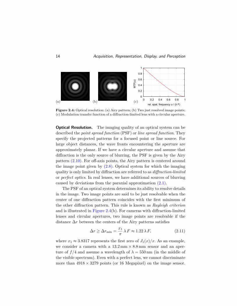
Figure 2.4: Optical resolution: (a) Airy pattern; (b) Two just resolved image points;(c) Modulation transfer function of a diffraction-limited lens with a circular aperture.
Optical Resolution. The imaging quality of an optical system can bedescribed the point spread function (PSF) or line spread function. Theyspecify the projected patterns for a focused point or line source. Forlarge object distances, the wave fronts encountering the aperture areapproximately planar. If we have a circular aperture and assume thatdiffraction is the only source of blurring, the PSF is given by the Airypattern (2.10). For off-axis points, the Airy pattern is centered aroundthe image point given by (2.8). Optical system for which the imagingquality is only limited by diffraction are referred to as diffraction-limitedor perfect optics. In real lenses, we have additional sources of blurringcaused by deviations from the paraxial approximation (2.1).
The PSF of an optical system determines its ability to resolve detailsin the image. Two image points are said to be just resolvable when thecenter of one diffraction pattern coincides with the first minimum ofthe other diffraction pattern. This rule is known as Rayleigh criterionand is illustrated in Figure 2.4(b). For cameras with diffraction-limitedlenses and circular apertures, two image points are resolvable if thedistance ∆r between the centers of the Airy patterns satisfies
∆r ≥ ∆rmin = x1πλF ≈ 1.22λF, (2.11)
where x1 ≈ 3.8317 represents the first zero of J1(x)/x. As an example,we consider a camera with a 13.2 mm× 8.8 mm sensor and an aper-ture of f/4 and assume a wavelength of λ = 550nm (in the middle ofthe visible spectrum). Even with a perfect lens, we cannot discriminatemore than 4918× 3279 points (or 16 Megapixel) on the image sensor.

2.1. Fundamentals of Image Formation 15
The number of discriminable points increases with decreasing f-numberand increasing sensor size. By considering (2.7), we can, however, con-clude that for a given picture (same field of view and depth of field),the number of distinguishable points is independent of the sensor size.
Modulation Transfer Function. The resolving capabilities of lensesare often specified in the frequency domain. The optical transfer func-tion (OTF) is defined as the two-dimensional Fourier transform ofthe point spread function, OTF(u, v) = FT{PSF(x, y)}. The amplitudespectrum MTF(u, v) = |OTF(u, v)| is referred to as modulation trans-fer function (MTF). Typically, only a one-dimensional slice MTF(u)of the modulation transfer function MTF(u, v) is considered, whichcorresponds to the Fourier transform of the line spread function. Thecontrast C of an irradiance pattern shall be defined by
C = Imax − IminImax + Imin
, (2.12)
where Imin and Imax represent the minimum and maximum irradiances.The modulation transfer MTF(u) specifies the reduction in contrast Cfor harmonic stimuli with a spatial frequency u,
MTF(u) = Cimage /Cobject, (2.13)
where Cobject and Cimage denote the contrasts in the object and imagedomain, respectively. The OTF of diffraction-limited optics can alsobe calculated as the normalized autocorrelation function of the pupilfunction g(ζ, η) [28]. For a camera with a diffraction-limited lens anda circular aperture with the f-number F , the MTF is given by
MTF(u) =
2π
(arccos u
u0− u
u0
√1−
(uu0
)2)
: u ≤ u0
0 : u > u0
, (2.14)
where u0 = 1/(λF ) represents the cut-off frequency. This function isillustrated in Figure 2.4(c). The MTF for real lenses generally lies be-low that for diffraction-limited optics. Furthermore, for real lenses, theMTF additionally depends on the position in the image plane and theorientation of the harmonic pattern.

16 Acquisition, Representation, Display, and Perception
(a) (b) (c)
(1)
(2)(d) (e) (f)
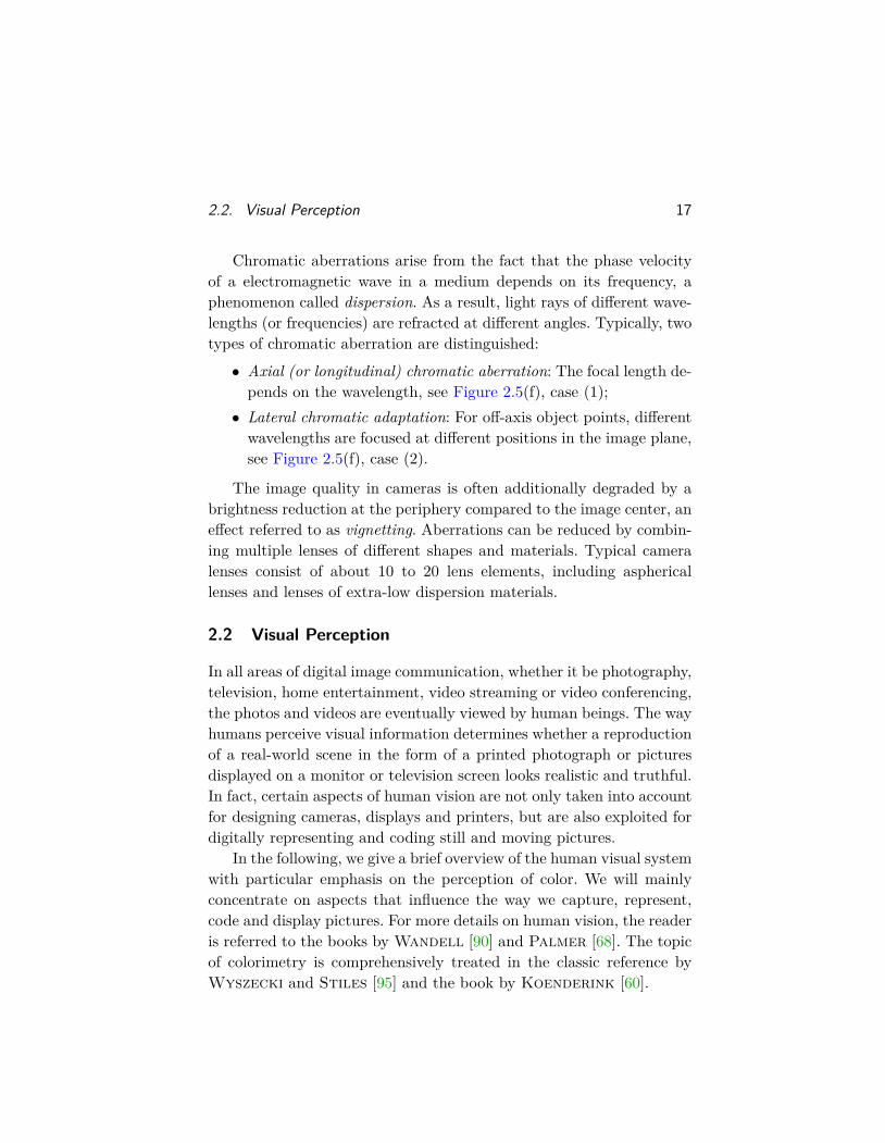
Figure 2.5: Aberrations: (a) Spherical Aberration; (b) Field curvature; (c) Coma;(d) Astigmatism; (e) Distortion; (f) Axial(1) and lateral(2) chromatic aberration.
2.1.3 Optical Aberrations
We analyzed aspects of the image formation with lenses using the Gaus-sian lens formula (2.1). Since this formula represents only an approxi-mation for thin lenses and paraxial rays, it does not provide an accuratedescription of real lenses. Deviations from the predictions of Gaussianoptics that are not caused by diffraction are called aberrations. Thereare two main classes of aberrations: Monochromatic aberrations, whichare caused by the geometry of lenses and occur even with monochro-matic light, and chromatic aberrations, which occur only for light con-sisting of multiple wavelengths. The five primary monochromatic aber-rations, which are also called Seidel aberrations, are:
• Spherical aberration: The focal point of light rays depends ontheir distance to the optical axis, see Figure 2.5(a);• Field curvature: Points in a flat object plane are focused in acurved surface instead of a flat image plane, see Figure 2.5(b);• Coma: The projections of off-axis object points appear as a comet-shaped blur spots instead of points, see Figure 2.5(c);
• Astigmatism: Light rays that propagate in perpendicular planesare focused in different distances, see Figure 2.5(d);• Distortion: Straight lines in the object plane appear as curvedlines in the image plane, objects are deformed, see Figure 2.5(e).
2.2. Visual Perception 17
Chromatic aberrations arise from the fact that the phase velocityof a electromagnetic wave in a medium depends on its frequency, aphenomenon called dispersion. As a result, light rays of different wave-lengths (or frequencies) are refracted at different angles. Typically, twotypes of chromatic aberration are distinguished:
• Axial (or longitudinal) chromatic aberration: The focal length de-pends on the wavelength, see Figure 2.5(f), case (1);
• Lateral chromatic adaptation: For off-axis object points, differentwavelengths are focused at different positions in the image plane,see Figure 2.5(f), case (2).
The image quality in cameras is often additionally degraded by abrightness reduction at the periphery compared to the image center, aneffect referred to as vignetting. Aberrations can be reduced by combin-ing multiple lenses of different shapes and materials. Typical cameralenses consist of about 10 to 20 lens elements, including asphericallenses and lenses of extra-low dispersion materials.
2.2 Visual Perception
In all areas of digital image communication, whether it be photography,television, home entertainment, video streaming or video conferencing,the photos and videos are eventually viewed by human beings. The wayhumans perceive visual information determines whether a reproductionof a real-world scene in the form of a printed photograph or picturesdisplayed on a monitor or television screen looks realistic and truthful.In fact, certain aspects of human vision are not only taken into accountfor designing cameras, displays and printers, but are also exploited fordigitally representing and coding still and moving pictures.
In the following, we give a brief overview of the human visual systemwith particular emphasis on the perception of color. We will mainlyconcentrate on aspects that influence the way we capture, represent,code and display pictures. For more details on human vision, the readeris referred to the books by Wandell [90] and Palmer [68]. The topicof colorimetry is comprehensively treated in the classic reference byWyszecki and Stiles [95] and the book by Koenderink [60].
18 Acquisition, Representation, Display, and Perception
crystalline lensretina
fovea
optic nerve
ciliary muscle
iris
pupil
cornea
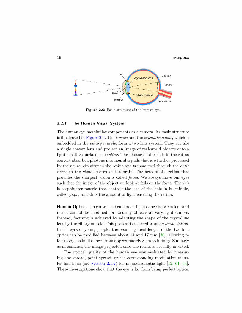
Figure 2.6: Basic structure of the human eye.
2.2.1 The Human Visual System
The human eye has similar components as a camera. Its basic structureis illustrated in Figure 2.6. The cornea and the crystalline lens, which isembedded in the ciliary muscle, form a two-lens system. They act likea single convex lens and project an image of real-world objects onto alight-sensitive surface, the retina. The photoreceptor cells in the retinaconvert absorbed photons into neural signals that are further processedby the neural circuitry in the retina and transmitted through the opticnerve to the visual cortex of the brain. The area of the retina thatprovides the sharpest vision is called fovea. We always move our eyessuch that the image of the object we look at falls on the fovea. The irisis a sphincter muscle that controls the size of the hole in its middle,called pupil, and thus the amount of light entering the retina.
Human Optics. In contrast to cameras, the distance between lens andretina cannot be modified for focusing objects at varying distances.Instead, focusing is achieved by adapting the shape of the crystallinelens by the ciliary muscle. This process is referred to as accommodation.In the eyes of young people, the resulting focal length of the two-lensoptics can be modified between about 14 and 17 mm [30], allowing tofocus objects in distances from approximately 8 cm to infinity. Similarlyas in cameras, the image projected onto the retina is actually inverted.
The optical quality of the human eye was evaluated by measur-ing line spread, point spread, or the corresponding modulation trans-fer functions (see Section 2.1.2) for monochromatic light [12, 61, 64].These investigations show that the eye is far from being perfect optics.
2.2. Visual Perception 19
0° (fovea)
−20°
40°60°80°
20°
−40°−60°−80°
nasal
temporal
0 2 4 6 8
10 12 14 16 18 20
-60 -40 -20 0 20 40
rece
ptor
den
sity
[104
/ mm2 ]
visual angle relative to center of fovea [degree]
blind spot
nasal retina temporal retina
rodscones
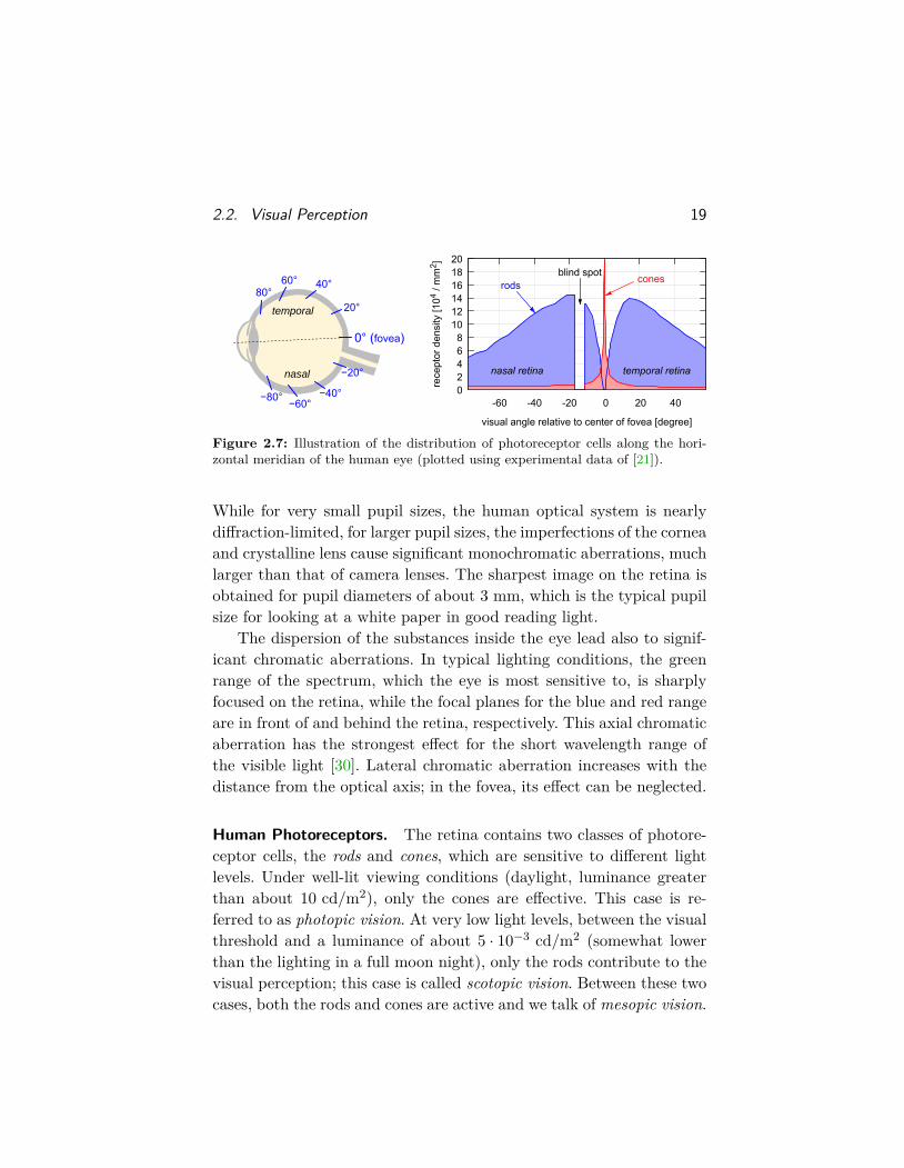
Figure 2.7: Illustration of the distribution of photoreceptor cells along the hori-zontal meridian of the human eye (plotted using experimental data of [21]).
While for very small pupil sizes, the human optical system is nearlydiffraction-limited, for larger pupil sizes, the imperfections of the corneaand crystalline lens cause significant monochromatic aberrations, muchlarger than that of camera lenses. The sharpest image on the retina isobtained for pupil diameters of about 3 mm, which is the typical pupilsize for looking at a white paper in good reading light.
The dispersion of the substances inside the eye lead also to signif-icant chromatic aberrations. In typical lighting conditions, the greenrange of the spectrum, which the eye is most sensitive to, is sharplyfocused on the retina, while the focal planes for the blue and red rangeare in front of and behind the retina, respectively. This axial chromaticaberration has the strongest effect for the short wavelength range ofthe visible light [30]. Lateral chromatic aberration increases with thedistance from the optical axis; in the fovea, its effect can be neglected.
Human Photoreceptors. The retina contains two classes of photore-ceptor cells, the rods and cones, which are sensitive to different lightlevels. Under well-lit viewing conditions (daylight, luminance greaterthan about 10 cd/m2), only the cones are effective. This case is re-ferred to as photopic vision. At very low light levels, between the visualthreshold and a luminance of about 5 · 10−3 cd/m2 (somewhat lowerthan the lighting in a full moon night), only the rods contribute to thevisual perception; this case is called scotopic vision. Between these twocases, both the rods and cones are active and we talk of mesopic vision.
20 Acquisition, Representation, Display, and Perception
There are about 100 million rods and 5 million cones in each eye,which are very differently distributed throughout the retina [67, 21],see Figure 2.7. The rods are mainly concentrated in the periphery. Thefovea does not contain any rods, but by far the highest concentration ofcones. At the location of the optic nerve, also referred to as blind spot,there are no photoreceptors. Although the retina contains much morerods than cones, the visual acuity of scotopic vision is much lower thanthat of photopic version. The reason is that the photocurrent responsesof many rods are combined into a single neural response, whereas eachcone signal is further processed by several neurons in the retina [90].
Spectral Sensitivity. The sensitivity of the human eye depends onthe spectral characteristics of the observed light stimulus. Based onthe data of several brightness-matching experiments, for example [27],the Commission Internationale de l’Eclairage (CIE) defined the so-called CIE luminous efficiency function V (λ) for photopic vision [14]in 1924. This function characterizes the average spectral sensitivity ofhuman brightness perception1. Two light stimuli with different radiancespectra Φ(λ) are perceived as equally bright if the corresponding values∫∞
0 Φ(λ)V (λ) dλ are the same. V (λ) determines the relation betweenradiometric and photometric quantities. For example, the analogousphotometric quantity of the radiance Φ=
∫∞0 Φ(λ) dλ is the luminance
I =K∫∞
0 V (λ)Φ(λ) dλ, where K is a constant (683 lumen per Watt).The SI unit of the luminance is candela per square meter (cd/m2).
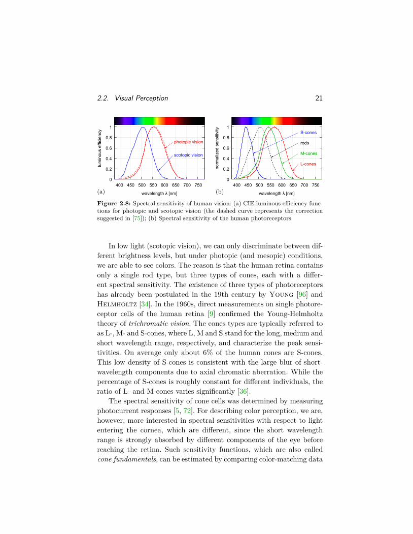
Viewing experiments under scotopic conditions lead to the defini-tion of a scotopic luminous efficiency function V ′(λ) [16]. The luminousefficiency functions V (λ) and V ′(λ) are depicted in Figure 2.8(a). Thephenomenon that the wavelength range of highest sensitivity is differ-ent for photopic and scotopic vision is referred to as the Purkinje effect.Both luminous efficiency functions are noticeably greater than zero inthe range from about 390 to 700 nm. For that reason, electromagneticradiation in this part of the spectrum is commonly called visible light.
1The CIE 1924 photopic luminous efficiency function V (λ) has been reported tounderestimate the contribution of the short wavelength range. Improvements weresuggested by Judd [56], Vos [89], and more recently by Sharpe et al. [74, 75].
2.2. Visual Perception 21
0
0.2
0.4
0.6
0.8
1
400 450 500 550 600 650 700 750
lum
inou
s ef
ficie
ncy
wavelength λ [nm]
photopic vision
scotopic vision
0
0.2
0.4
0.6
0.8
1
400 450 500 550 600 650 700 750
norm
aliz
ed s
ensi
tivity
wavelength λ [nm]
S-cones
rods
M-cones
L-cones
(a) (b)
Figure 2.8: Spectral sensitivity of human vision: (a) CIE luminous efficiency func-tions for photopic and scotopic vision (the dashed curve represents the correctionsuggested in [75]); (b) Spectral sensitivity of the human photoreceptors.
In low light (scotopic vision), we can only discriminate between dif-ferent brightness levels, but under photopic (and mesopic) conditions,we are able to see colors. The reason is that the human retina containsonly a single rod type, but three types of cones, each with a differ-ent spectral sensitivity. The existence of three types of photoreceptorshas already been postulated in the 19th century by Young [96] andHelmholtz [34]. In the 1960s, direct measurements on single photore-ceptor cells of the human retina [9] confirmed the Young-Helmholtztheory of trichromatic vision. The cones types are typically referred toas L-, M- and S-cones, where L, M and S stand for the long, medium andshort wavelength range, respectively, and characterize the peak sensi-tivities. On average only about 6% of the human cones are S-cones.This low density of S-cones is consistent with the large blur of short-wavelength components due to axial chromatic aberration. While thepercentage of S-cones is roughly constant for different individuals, theratio of L- and M-cones varies significantly [36].
The spectral sensitivity of cone cells was determined by measuringphotocurrent responses [5, 72]. For describing color perception, we are,however, more interested in spectral sensitivities with respect to lightentering the cornea, which are different, since the short wavelengthrange is strongly absorbed by different components of the eye beforereaching the retina. Such sensitivity functions, which are also calledcone fundamentals, can be estimated by comparing color-matching data
22 Acquisition, Representation, Display, and Perception
(see Section 2.2.2) of individuals with normal vision with that of in-dividuals lacking one or two cone types. In Figure 2.8(b), the conefundamentals estimated by Stockman et al. [82, 81] are depictedtogether with the spectral sensitivity function for the rods, which isthe same as the scotopic luminous efficiency function V ′(λ).
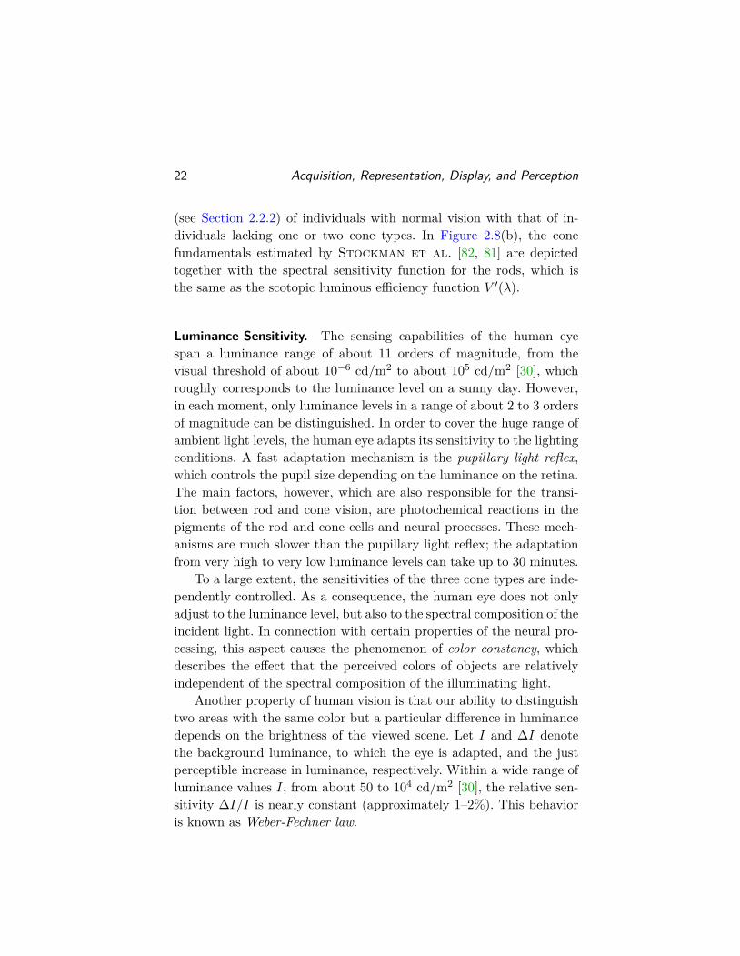
Luminance Sensitivity. The sensing capabilities of the human eyespan a luminance range of about 11 orders of magnitude, from thevisual threshold of about 10−6 cd/m2 to about 105 cd/m2 [30], whichroughly corresponds to the luminance level on a sunny day. However,in each moment, only luminance levels in a range of about 2 to 3 ordersof magnitude can be distinguished. In order to cover the huge range ofambient light levels, the human eye adapts its sensitivity to the lightingconditions. A fast adaptation mechanism is the pupillary light reflex,which controls the pupil size depending on the luminance on the retina.The main factors, however, which are also responsible for the transi-tion between rod and cone vision, are photochemical reactions in thepigments of the rod and cone cells and neural processes. These mech-anisms are much slower than the pupillary light reflex; the adaptationfrom very high to very low luminance levels can take up to 30 minutes.
To a large extent, the sensitivities of the three cone types are inde-pendently controlled. As a consequence, the human eye does not onlyadjust to the luminance level, but also to the spectral composition of theincident light. In connection with certain properties of the neural pro-cessing, this aspect causes the phenomenon of color constancy, whichdescribes the effect that the perceived colors of objects are relativelyindependent of the spectral composition of the illuminating light.
Another property of human vision is that our ability to distinguishtwo areas with the same color but a particular difference in luminancedepends on the brightness of the viewed scene. Let I and ∆I denotethe background luminance, to which the eye is adapted, and the justperceptible increase in luminance, respectively. Within a wide range ofluminance values I, from about 50 to 104 cd/m2 [30], the relative sen-sitivity ∆I/I is nearly constant (approximately 1–2%). This behavioris known as Weber-Fechner law.
2.2. Visual Perception 23
Opponent Colors. The theory of opponent colors was first formulatedby Hering [35]. He found that certain hues are never perceived tooccur together. While colors can be perceived as a combination of, forexample, yellow and red (orange), red and blue (purple), or green andblue (cyan), there are no colors that are perceived as a combination ofred and green or yellow and blue. Hering concluded that the humancolor perception includes a mechanism with bipolar responses to red-green and blue-yellow. These hue pairs are referred to as opponentcolors. According to the opponent color theory, any light stimulus isreceived as containing either a one or the other of the opponent colorpairs, or, if both contributions cancel out, none of them.
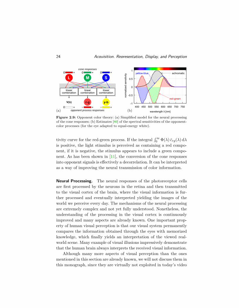
For a long time, the opponent color theory seemed to be irrecon-cilable with the Young-Helmholtz theory. In the 1950s, Jameson andHurvich [55, 37] performed hue-cancellation experiments by whichthey estimated the spectral sensitivities of the opponent-color mecha-nisms. Furthermore, measurements of electrical responses in the retinaof goldfish [83, 84] and the lateral geniculate nucleus of the macaquemonkey [23] showed the existence of neural signals that were consistentwith the bipolar responses formulated by Hering. These and otherexperimental findings resulted in a wide acceptance of the modern the-ory of opponent colors, according to which the responses of the threecones to light stimuli are not directly transmitted to the brain. Instead,neurons along the visual pathways transform the cone responses intothree opponent signals, as illustrated in Figure 2.9(a). The transforma-tion can be considered as approximately linear and the outputs are anachromatic signal, which corresponds to a relative luminance measure,as well as a red-green and a yellow-blue color difference signal.
Since the cone sensitivities are to a large extent independently ad-justed, the spectral sensitivities of the opponent processes depend onthe present illumination. Estimates of the spectral sensitivity curves forthe eye adapted to equal-energy white (same spectral radiance for allwavelengths) are shown in Figure 2.9(b). The depicted curves representlinear combinations, suggested in [80], of the Stockman and Sharpecone fundamentals [81]. As an example, let Φ(λ) denote the radiancespectrum of a light stimulus and let crg(λ) represent the spectral sensi-
24 Acquisition, Representation, Display, and Perception
linearcombination
linearcombination
linearcombination
r-g− +
y-b− +
V(λ)
0 +
L0 +
M0 +
S0 +
cone responses
opponent process responses
-1
-0.5
0
0.5
1
400 450 500 550 600 650 700 750
norm
aliz
ed s
ensi
tivity
wavelength λ [nm]
yellow-blue
red-green
achromatic
(a) (b)
Figure 2.9: Opponent color theory: (a) Simplified model for the neural processingof the cone responses; (b) Estimates [80] of the spectral sensitivities of the opponent-color processes (for the eye adapted to equal-energy white).
tivity curve for the red-green process. If the integral∫∞
0 Φ(λ) crg(λ) dλis positive, the light stimulus is perceived as containing a red compo-nent, if it is negative, the stimulus appears to include a green compo-nent. As has been shown in [11], the conversion of the cone responsesinto opponent signals is effectively a decorrelation. It can be interpretedas a way of improving the neural transmission of color information.
Neural Processing. The neural responses of the photoreceptor cellsare first processed by the neurons in the retina and then transmittedto the visual cortex of the brain, where the visual information is fur-ther processed and eventually interpreted yielding the images of theworld we perceive every day. The mechanisms of the neural processingare extremely complex and not yet fully understood. Nonetheless, theunderstanding of the processing in the visual cortex is continuouslyimproved and many aspects are already known. One important prop-erty of human visual perception is that our visual system permanentlycompares the information obtained through the eyes with memorizedknowledge, which finally yields an interpretation of the viewed real-world scene. Many example of visual illusions impressively demonstratethat the human brain always interprets the received visual information.
Although many more aspects of visual perception than the onesmentioned in this section are already known, we will not discuss them inthis monograph, since they are virtually not exploited in today’s video

2.2. Visual Perception 25
communication applications. The main reason that most properties ofhuman vision are neglected in image and video coding is that no simpleand sufficiently accurate model has been found that allows to quantifythe perceived image quality based on samples of an image or video.
2.2.2 Color Perception
While the previous section gave a brief overview of the human visualsystem, we will now further analyze and quantitatively describe theperception and reproduction of color information. In particular, we willdiscuss the colorimetric standards of the CIE, which are widely usedas basis for specifying color in image and video representation formats.
Metamers. It is a well-known fact that, by using a prism, a ray ofsunlight can be split into components of different wavelengths, whichwe perceive to have different colors, ranging from violet over blue, cyan,green, yellow, orange to red. We can conclude that light with a partic-ular spectral composition induces the perception of a particular color,but the converse is not true. Two light stimuli that appear to have thesame color can have very different spectral compositions. Color is not aphysical quantity, but a sensation in the viewers mind induced by theinteraction of electromagnetic waves with the human cones.
A light stimulus emitted or reflected from the surface of an objectand falling through the pupil of the eye can be physically characterizedby its radiance spectrum, specifying its composition of electromagneticwaves with different wavelengths. The light falling on the retina excitesthe three cone types in different ways. Let l(λ), m(λ) and s(λ) representthe normalized spectral sensitivity curves of the L-, M- and S-cones,respectively, which have been illustrated in Figure 2.8. Then, a radiancespectrum Φ(λ) is effectively mapped to a three-dimensional vectorLM
S
=∞∫
0
¯(λ)m(λ)s(λ)
Φ(λ)Φ0
dλ, (2.15)
where Φ0>0 represents an arbitrarily chosen reference radiance, whichis introduced for making the vector (L,M,S) dimensionless.
26 Acquisition, Representation, Display, and Perception
0
0.2
0.4
0.6
0.8
1
400 450 500 550 600 650 700 750
spec
tral
rad
ianc
e Φ
(λ)
/ Φmax
wavelength λ [nm]
Φ1(λ)
Φ2(λ)
Φ3(λ)
Φ4(λ)perceived color:
orange
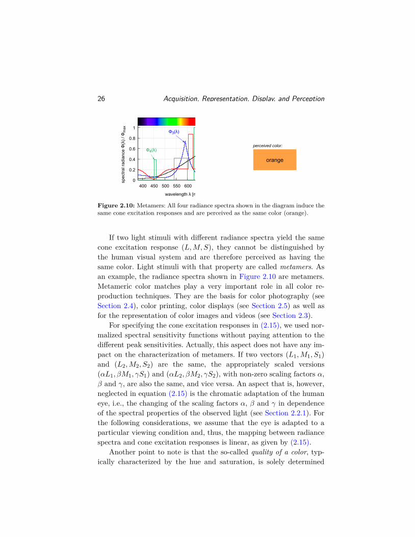
Figure 2.10: Metamers: All four radiance spectra shown in the diagram induce thesame cone excitation responses and are perceived as the same color (orange).
If two light stimuli with different radiance spectra yield the samecone excitation response (L,M,S), they cannot be distinguished bythe human visual system and are therefore perceived as having thesame color. Light stimuli with that property are called metamers. Asan example, the radiance spectra shown in Figure 2.10 are metamers.Metameric color matches play a very important role in all color re-production techniques. They are the basis for color photography (seeSection 2.4), color printing, color displays (see Section 2.5) as well asfor the representation of color images and videos (see Section 2.3).
For specifying the cone excitation responses in (2.15), we used nor-malized spectral sensitivity functions without paying attention to thedifferent peak sensitivities. Actually, this aspect does not have any im-pact on the characterization of metamers. If two vectors (L1,M1, S1)and (L2,M2, S2) are the same, the appropriately scaled versions(αL1, βM1, γS1) and (αL2, βM2, γS2), with non-zero scaling factors α,β and γ, are also the same, and vice versa. An aspect that is, however,neglected in equation (2.15) is the chromatic adaptation of the humaneye, i.e., the changing of the scaling factors α, β and γ in dependenceof the spectral properties of the observed light (see Section 2.2.1). Forthe following considerations, we assume that the eye is adapted to aparticular viewing condition and, thus, the mapping between radiancespectra and cone excitation responses is linear, as given by (2.15).
Another point to note is that the so-called quality of a color, typ-ically characterized by the hue and saturation, is solely determined
2.2. Visual Perception 27
by the ratio L :M :S. Two colors given by the cone response vectors(L1,M1, S1) and (L2,M2, S2) = (αL1, αM1, αS1), with α > 1, have thesame quality, i.e., the same hue and saturation, but the luminance2 ofthe color (L2,M2, S2) is by a factor of α larger than that of (L1,M1, S1).
Although (2.15) could be directly used for quantifying the percep-tion of color, the colorimetric standards are based on empirical dataobtained in color-matching experiments. One reason is that the spectralsensitivities of the human cones had not be known at the time whenthe standards were developed. Actually, the cone fundamentals are typ-ically estimated based on data of color-matching experiments [81].
Mixing of Primary Colors. Since the perceived color of a light stim-ulus can be represented by three cone excitation levels, it seems likelythat, for each radiance spectrum Φ(λ), we can also create a metamericspectrum Φ∗(λ) by suitably mixing three primary colors or, more cor-rectly, primary lights. The radiance spectra of the three primary lightsA, B and C shall be given by pA(λ), pB(λ) and pC(λ), respectively. Withp(λ) = ( pA(λ), pB(λ), pC(λ) )T, the radiance spectrum of a mixture ofthe primaries A, B and C is given by
Φ∗(λ) = A · pA(λ) +B · pB(λ) + C · pC(λ) = (A,B,C) · p(λ), (2.16)
where A, B and C denote the mixing factors, which are also referred toas tristimulus values. The radiance spectrum Φ∗(λ) of the light mixtureis a metamer of Φ(λ) if and only if it yields the same cone excitationresponses. Thus, with (L,M,S) being the vector of cone excitationresponses for Φ(λ), we requireLM
S
=∞∫
0
¯(λ)m(λ)s(λ)
Φ∗(λ)Φ0
dλ = T ·
ABC
, (2.17)
with the transformation matrix T being given by
T =∞∫
0
¯(λ)m(λ)s(λ)
p(λ)T
Φ0dλ. (2.18)
2As mentioned in Section 2.2.1, we assume that the luminance can be representedas a linear combination of the cone excitation responses L, M , and S.
28 Acquisition, Representation, Display, and Perception
If the primaries are selected in a way that the matrix T is invertible,the mapping between the tristimulus values (A,B,C) and (L,M,S) isbijective. In this case, the color of each possible radiance spectrum Φ(λ)can be matched by a mixture of the three primary lights. And there-fore, the color description in the (A,B,C) system is equivalent to thedescription in the (L,M,S) system. A sufficient condition for a suit-able selection of the three primaries is that all primaries are perceivedas having a different color and the color of none of the primaries canbe matched by a mixture of the two other primaries. One aspect thatwill be discussed later, but should be noted at this point, is that foreach selection of real primaries, i.e., primaries with radiance spectrap(λ) ≥ 0, ∀λ, there are stimuli Φ(λ) for which one or two of the mixingfactors A, B and C are negative.
By combining the equations (2.17) and (2.15), we obtainABC
= T−1
LMS
= T−1∞∫
0
¯(λ)m(λ)s(λ)
Φ(λ)Φ0
dλ =∞∫
0
c(λ)Φ(λ)Φ0
dλ, (2.19)
which specifies the direct mapping of radiance spectra Φ(λ) onto thetristimulus values (A,B,C). The components a(λ), b(λ) and c(λ) ofthe vector function c(λ) = ( a(λ), b(λ), c(λ) )T are referred to as color-matching functions for the primaries A, B and C, respectively. Theyrepresent equivalents to the cone fundamentals ¯(λ), m(λ) and s(λ).Thus, if we know the color-matching functions a(λ), b(λ) and c(λ) fora set of three primaries, we can uniquely describe all perceivable colorsby the corresponding tristimulus values (A,B,C).
Before we discuss how color-matching functions can be determined,we highlight an important property of color mixing, which is a directconsequence of (2.19). Let Φ1(λ) and Φ2(λ) be the radiance spectraof two lights with the tristimulus values (A1, B1, C1) and (A2, B2, C2),respectively. Now, we mix an amount α of the first with an amount βof the second light. For the tristimulus values (A,B,C) of the resultingradiance spectrum Φ(λ) = αΦ1(λ) + β Φ2(λ), we obtainAB
C
=∞∫
0
c(λ) αΦ1(λ) + βΦ2(λ)Φ0
dλ = α
A1B1C1
+ β
A2B2C2
. (2.20)
2.2. Visual Perception 29
observation
screen
masking
screen
primary
lights
test
light
observer
2°
image seen
by observer
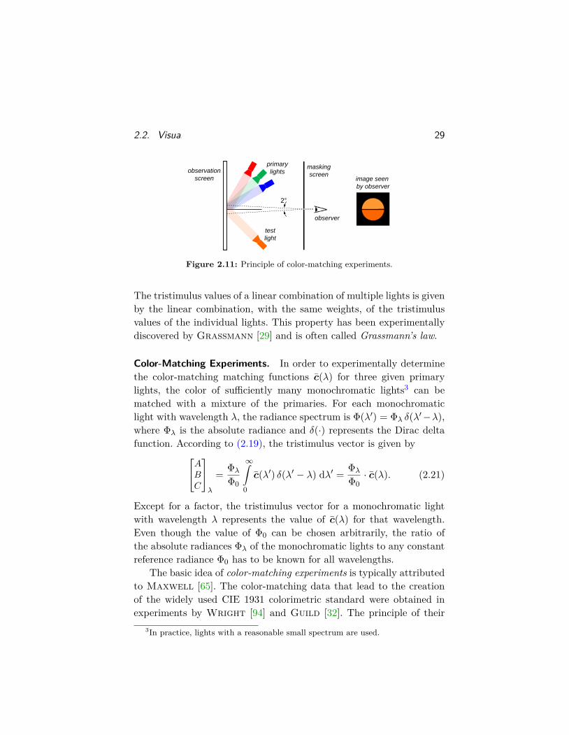
Figure 2.11: Principle of color-matching experiments.
The tristimulus values of a linear combination of multiple lights is givenby the linear combination, with the same weights, of the tristimulusvalues of the individual lights. This property has been experimentallydiscovered by Grassmann [29] and is often called Grassmann’s law.
Color-Matching Experiments. In order to experimentally determinethe color-matching matching functions c(λ) for three given primarylights, the color of sufficiently many monochromatic lights3 can bematched with a mixture of the primaries. For each monochromaticlight with wavelength λ, the radiance spectrum is Φ(λ′) = Φλ δ(λ′−λ),where Φλ is the absolute radiance and δ(·) represents the Dirac deltafunction. According to (2.19), the tristimulus vector is given byAB
C
λ
= Φλ
Φ0
∞∫0
c(λ′) δ(λ′ − λ) dλ′ = Φλ
Φ0· c(λ). (2.21)
Except for a factor, the tristimulus vector for a monochromatic lightwith wavelength λ represents the value of c(λ) for that wavelength.Even though the value of Φ0 can be chosen arbitrarily, the ratio ofthe absolute radiances Φλ of the monochromatic lights to any constantreference radiance Φ0 has to be known for all wavelengths.
The basic idea of color-matching experiments is typically attributedto Maxwell [65]. The color-matching data that lead to the creationof the widely used CIE 1931 colorimetric standard were obtained inexperiments by Wright [94] and Guild [32]. The principle of their
3In practice, lights with a reasonable small spectrum are used.
30 Acquisition, Representation, Display, and Perception
color-matching experiments [31, 93] is illustrated in Figure 2.11. Ata visual angle of 2◦, the observers looked at both a monochromatictest light and a mixture of the three primaries, for which a red, green,and blue light source were used. The amounts of the primaries could beadjusted by the observers. Since not all lights can be matched with pos-itive amounts of the primary lights, it was possible to move any of theprimaries to the side of the test light, in which case the amount of thecorresponding primary was counted as negative value4. The monochro-matic lights were obtained by splitting a beam of white light using aprism and selecting a small portion of the spectrum using a thin slit.
For determining the color-matching functions c(λ), only the ratiosof the amounts of the primary lights were utilized. These data werecombined with the already estimated luminous efficiency function V (λ)for photopic vision, assuming that V (λ) can be represented as linearcombination of the three color-matching functions a(λ), b(λ) and c(λ).Due to the linear relationship between the tristimulus values (A,B,C)and the cone response vectors (L,M,S), the assumption is equivalent tothe often used model (see Section 2.2.1) that the sensation of luminanceis generated by linearly combining the cone excitation responses in theneural circuitry of the human visual system. The utilization of theluminous efficiency function V (λ) had the advantage that the effect ofluminance perception could be excluded in the experiments and thatit was not necessary to know the ratios of the absolute radiances Φλ
to a common reference Φ0 for all monochromatic lights (see above).The exact mathematical procedure for determining the color-matchingfunctions c(λ) given the mixing ratios and V (λ) is described in [76].
Changing Primaries. Before we discuss the results of Wright andGuild, we consider how the color-matching functions for an arbitraryset of primaries can be derived from the measurements for anotherset of primaries. Let us assume that we measured the color-matchingfunctions c1(λ) = ( a1(λ), b1(λ), c1(λ) )T for a first set of primaries given
4Due to the linearity of color mixing, adding a particular amount of a primaryto the test light is mathematically equivalent to subtracting the same amount fromthe mixture of the other primaries.
2.2. Visual Perception 31
by the radiance spectra p1(λ) = ( pA1(λ), pB1(λ), pC1(λ) )T. Based onthese data, we want to determined the color-matching functions c2(λ)for a second set of primaries, which shall be given by the radiancespectra p2(λ). For each radiance spectrum Φ(λ), the tristimulus vectorst1 = (A1, B1, C1)T and t2 = (A2, B2, C2)T for the primary sets one andtwo, respectively, are given by
t1 =∞∫
0
c1(λ) Φ(λ)Φ0
dλ and t2 =∞∫
0
c2(λ) Φ(λ)Φ0
dλ . (2.22)
The radiance spectra Φ(λ), Φ1(λ) = p1(λ)Tt1 and Φ2(λ) = p2(λ)Tt2are metamers. Consequently, all three spectra correspond to the samecolor representation for any set of primaries. In particular, we require
t1 =∞∫
0
c1(λ) Φ2(λ)Φ0
dλ =
∞∫0
c1(λ) p2(λ)T
Φ0dλ
t2 = T 21 t2 . (2.23)
The tristimulus vector in one system of primaries can be converted intoany other system of primaries using a linear transformation. Since thisrelationship is valid for all radiance spectra Φ(λ), including those ofthe monochromatic lights, the color-matching functions for the secondset of primaries can be calculated according to
c2(λ) = T−121 c1(λ) = T 12 c1(λ) . (2.24)
It should be noted that the columns of a matrix T ik represent thetristimulus vectors (A,B,C) of the primary lights of set i in the primarysystem k. These values can be directly measured, so that the color-matching functions can be transformed from one into another primarysystem even if the radiance spectra p1(λ) and p2(λ) are unknown.
CIE Standard Colorimetric Observer. In 1931, the CIE adopted thecolorimetric standard known as CIE 1931 2◦ Standard ColorimetricObserver [15] based on the experimental data of Wright and Guild.Since Wright and Guild used different primaries in their experi-ments, the data had to be converted into a common primary system.For that purpose, monochromatic primaries with wavelengths of 700 nm
32 Acquisition, Representation, Display, and Perception
(red), 546.1 nm (green) and 435.8 nm (blue) were selected5. Since thetristimulus values for monochromatic lights had been measured in theexperiments, the conversion matrices could be derived by interpolatingthese data at the wavelengths of the new primary system. The ratio ofthe absolute radiances of the primary lights was decided to be chosenso that white light with a constant radiance spectrum is representedby equal amounts of all three primaries. Hence, the to-be-determinedcolor-matching functions r(λ), g(λ) and b(λ) for the red, green and blueprimaries, respectively, had to fulfill the condition
∞∫0
r(λ) dλ =∞∫
0
g(λ) dλ =∞∫
0
b(λ) dλ. (2.25)
The experimental data of Wright and Guild were transformed intothe new primary system, the results were averaged and some irregular-ities were removed [76, 8]. The requirement (2.25) resulted in a lumi-nance ratio IR :IG :IB equal to 1 :4.5907 :0.0601, where IR, IG and IBrepresent the luminances of the red, green and blue primaries, respec-tively. The corresponding ratio ΦR : ΦG : ΦB of the absolute radiancesis approximately 1:0.0191:0.0137. Finally, the normalization factor forthe color-matching functions, i.e., the ratio ΦR/Φ0, was chosen suchthat the condition
V (λ) = r(λ) + IGIR· g(λ) + IB
IR· b(λ) (2.26)
is fulfilled. The resulting CIE 1931 RGB color-matching functions r(λ),g(λ) and b(λ) were tabulated for wavelengths from 380 to 780 nm atintervals of 5 nm [15, 76]. They are shown in Figure 2.12(a). It is clearlyvisible, that r(λ) has negative values inside the range from 435.8 to546.1 nm. In fact, for most of the wavelengths inside the range of visiblelight, one of the color-matching functions is negative, meaning thatmost of the monochromatic lights cannot be represented by a physicallymeaningful mixture of the chosen red, green and blue primaries.
The CIE decided to develop a second set of color-matching functionsx(λ), y(λ), and z(λ), which are now known as CIE 1931 XYZ color-matching functions, as basis for their colorimetric standard. Since all
5The primaries were chosen to be producible in a laboratory.

2.2. Visual Perception 33
-0.1
0
0.1
0.2
0.3
0.4
400 450 500 550 600 650 700 750
tris
timul
us a
mpl
itude
s
wavelength λ [nm]
b- (λ)
g- (λ)
r- (λ)
B G R 0
0.5
1
1.5
2
400 450 500 550 600 650 700 750
tris
timul
us a
mpl
itude
s
wavelength λ [nm]
z- (λ)
y- (λ) x
- (λ)
(a) (b)
Figure 2.12: CIE 1931 color-matching functions: (a) RGB color-matching func-tions, the primaries are marked with R, G and B; (b) XYZ color-matching functions.
sets of color-matching functions are linearly dependent, x(λ), y(λ), andz(λ) had to obey the relationship x(λ)
y(λ)z(λ)
= T XYZ ·
r(λ)g(λ)b(λ)
, (2.27)
with T XYZ being an invertible, but otherwise arbitrary, transformationmatrix. For specifying the 3×3 matrix T XYZ, the following desirableproperties were considered:
• All values of x(λ), y(λ) and z(λ) were to be non-negative;• The color-matching function y(λ) was to be chosen equal to theluminous efficiency function V (λ) for photopic vision;• The scaling was to be chosen so that the tristimulus values foran equal-energy spectrum are equal to each other;• For the long wavelength range, the entries of the color-matchingfunction z(λ) were to be equal to zero;
• Subject to the above criteria, the area that physical meaningfulradiance spectra represent inside a plane given by a constant sumX + Y + Z was to be maximized.
By considering these design principles, the transformation matrix
T XYZ = 10.17697
0.49000 0.31000 0.200000.17697 0.81240 0.010630.00000 0.01000 0.99000
(2.28)
34 Acquisition, Representation, Display, and Perception
was adopted. A detailed description of how this matrix was derived canbe found in [76, 26]. The resulting XYZ color-matching functions x(λ),y(λ) and z(λ) are depicted in Figure 2.12(b). They have been tabulatedfor the range from 380 to 780 nm, in intervals of 5 nm, and specify theCIE 1931 standard colorimetric observer [15]. The color of a radiancespectrum Φ(λ) can be represented by the tristimulus valuesXY
Z
=∞∫
0
x(λ)y(λ)z(λ)
Φ(λ)Φ0
dλ. (2.29)
The reference radiance Φ0 is typically chosen in a way that X, Y , andZ lie in a range from 0 to 1 for the considered viewing condition. Notethat, due to the choice y(λ) = V (λ), the value Y represents a scaledand dimensionless version of the luminance I. It is correctly referred toas relative luminance, however, often the term “luminance” is used forboth the “absolute” luminance I and the relative luminance Y .
In the 1950s, Stiles and Burch [79] performed color-matching ex-periments for a visual angle of 10◦. Based on these results, the CIEdefined the CIE 1964 10◦ Supplementary Colorimetric Observer [17].The data by Stiles and Burch are considered as the most secure setof existing color-matching functions [7] and have been used as basisfor the Stockman and Sharpe cone fundamentals [81] and the recentCIE proposal [19] of physiologically relevant color-matching functions.Baylor, Nunn and Schnapf [5] measured direct photocurrent re-sponses in the cones of a monkey and could predict the color-matchingfunctions of Stiles and Burch with reasonable accuracy. Nonetheless,the CIE 1931 Standard Colorimetric Observer [15] is still used in mostapplications. The RGB and XYZ color-matching functions for the CIEstandard observers are included in the recent ISO/CIE standard oncolorimetry [41] and can also be downloaded from [40].
Chromaticity Diagram. The black curve in Figure 2.13(a) shows thelocus of monochromatic lights with a particular radiance in the XYZspace. The tristimulus values of all possible radiance spectra representlinear combinations, with non-negative weights, of the (X,Y, Z) valuesfor monochromatic lights. They are located inside a cone, which has its
2.2. Visual Perception 35
Y
X
Z(a)
Y
X
Z
1
1
1(b)
0
0.1
0.2
0.3
0.4
0.5
0.6
0.7
0.8
0.9
0 0.1 0.2 0.3 0.4 0.5 0.6 0.7 0.8
chro
mat
icity
y
chromaticity x
460470
480
490
500
510
520
530
540
550
560
570
580
590
600
610
620
EW R
G
B
spectral locus
purple line
(c)
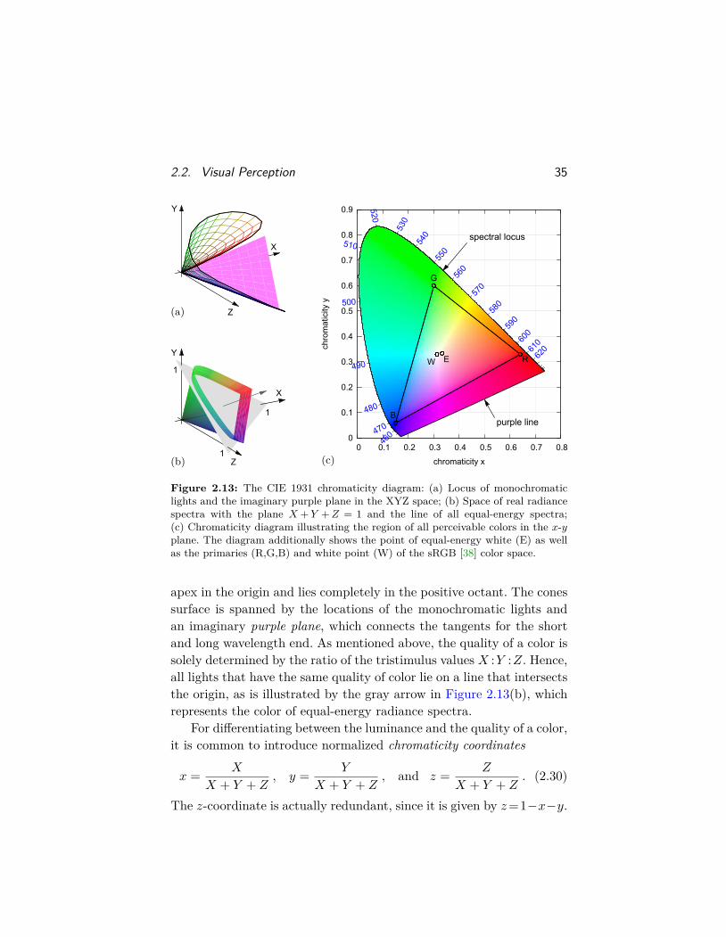
Figure 2.13: The CIE 1931 chromaticity diagram: (a) Locus of monochromaticlights and the imaginary purple plane in the XYZ space; (b) Space of real radiancespectra with the plane X +Y +Z = 1 and the line of all equal-energy spectra;(c) Chromaticity diagram illustrating the region of all perceivable colors in the x-yplane. The diagram additionally shows the point of equal-energy white (E) as wellas the primaries (R,G,B) and white point (W) of the sRGB [38] color space.
apex in the origin and lies completely in the positive octant. The conessurface is spanned by the locations of the monochromatic lights andan imaginary purple plane, which connects the tangents for the shortand long wavelength end. As mentioned above, the quality of a color issolely determined by the ratio of the tristimulus values X :Y :Z. Hence,all lights that have the same quality of color lie on a line that intersectsthe origin, as is illustrated by the gray arrow in Figure 2.13(b), whichrepresents the color of equal-energy radiance spectra.
For differentiating between the luminance and the quality of a color,it is common to introduce normalized chromaticity coordinates
x = X
X + Y + Z, y = Y
X + Y + Z, and z = Z
X + Y + Z. (2.30)
The z-coordinate is actually redundant, since it is given by z=1−x−y.
36 Acquisition, Representation, Display, and Perception
The tristimulus values (X,Y, Z) of a color can be represented by thechromaticity coordinates x and y, which specify the quality of the color,and the relative luminance Y . For a given quality of color, i.e., a ratioX : Y : Z, the chromaticity coordinates x and y correspond to thevalues of X and Y , respectively, inside the plane X + Y + Z = 1, asis illustrated in Figure 2.13(b). The set of qualities of colors that isperceivable by human beings is called the human gamut. Its locationin the x-y coordinate system is shown in Figure 2.13(c)6. This plotis referred to as chromaticity diagram. The human gamut representsa horseshoe shape; its boundaries are given by the projection of themonochromatic lights, referred to as spectral locus, and the purple line,which is a projection of the imaginary purple plane. For the spectrallocus, the figure includes wavelength labels in nanometers; it also showsthe location x = y = 1/3, marked by “E”, of equal-energy spectra.
Linear Color Spaces. All color spaces that are linearly related to theLMS cone excitation space shall be called linear color spaces in thismonograph. When neglecting measurement errors, the CIE RGB andXYZ spaces are linear color spaces and, hence, there exists a matrix bywhich the XYZ (or RGB) color-matching functions are transformed intocone fundamentals according to (2.24). Actually, cone fundamentals aretypically obtained by estimating such a transformation matrix [81].
While we specified the primary spectra for the CIE 1931 RGBcolor space, the color-matching functions for the CIE 1931 XYZ colorspace were derived by defining a transformation matrix, without ex-plicitly stating the primary spectra. Given the color-matching func-tions c(λ) = ( x(λ), y(λ), z(λ) )T, the corresponding primary spectrap(λ) = ( pX(λ), pY (λ), pZ(λ) )T are not uniquely defined. With I de-noting the 3×3 identify matrix, they only have to fulfill the condition
∞∫0
c(λ) p(λ)T dλ = Φ0 · I, (2.31)
6The complete human gamut cannot be reproduced on a display or in a print andthe perception of a color depends on the illumination conditions. Thus, the colorsshown in Figure 2.13(c) should be interpreted as a rough illustration.
2.2. Visual Perception 37
which is a special case of (2.23). Even though there are infinitely manyspectra p(λ) that fulfill (2.31), they all have negative entries and, thus,represent imaginary primaries7. The same is true for the LMS colorspace and all other linear color spaces with non-negative color-matchingfunctions. It is often referred to as primary paradoxon and is caused bythe fact that the cone fundamentals have overlapping support. Thereis no physical meaningful radiance spectrum, i.e., with p(λ) ≥ 0, ∀λ,that excites the M-cones without also exciting the L- or S-cones.
For all real primaries, the corresponding color-matching functionshave negative entries. Consequently, not all colors of the human gamutcan be represented by a physical meaningful mixture of the primarylights. As an example, the chromaticity diagram in Figure 2.13(c) showsthe chromaticity coordinates for the sRGB primaries [38]. Displays thatuse primaries with these chromaticity coordinates can only representthe colors that are located inside the triangle spanned by the primaries.This set of colors is called the color gamut of the display device.
In cameras, the situation is different. Since the transmittance spec-tra of the color filters (see Section 2.4), which represent the color-matching functions of the camera color space, are always non-negative,it is, in principle, possible to capture all colors of the human gamut.However, the camera color space is only a linear color space, if the trans-mittance spectra of the color filters represent linear combinations ofthe cone fundamentals (or, equivalently, the XYZ color-matching func-tions). In practice, this can be only approximately realized. Nonethe-less, often a linear transformation is used for converting the cameradata into a linear color space; a suitable transformation matrix can bedetermined by least-squares linear regression.
Since camera color spaces are associated with imaginary primaries,the image data captured by a camera sensor cannot be directly usedfor operating a display device, they always have to be converted. Sev-eral algorithms have been developed for realizing such a conversion; the
7This can be verified as follows. For obtaining∫y(λ)pY (λ)dλ=Φ0, the spectrum
pY (λ) has to contain values greater than 0 inside the range for which y(λ) is greaterthan 0, but since either x(λ) or z(λ) are also greater than 0 inside this range, theintegrals
∫x(λ)pY (λ)dλ and
∫z(λ)pY (λ)dλ cannot become equal to 0, unless pY (λ)
has also negative entries.
38 Acquisition, Representation, Display, and Perception
simplest variant consists of a linear transformation of the tristimulusvalues (for changing the primaries) and a subsequent clipping of nega-tive values. For the transmission between the camera and the display,an image or video representation format, such as the above mentionedsRGB, is used. Typically, the representation formats define linear RGBcolor spaces, for which the primary chromaticity coordinates lie in-side the human gamut and they only allow positive tristimulus values.Hence, the color spaces of representation formats also have a limitedcolor gamut, as has been shown for the sRGB format in Figure 2.13(c).
The conversion between an RGB and the XYZ color space can bewritten as XY
Z
=
Xr Xg Xb
Yr Yg Yb
Zr Zg Zb
·RGB
, (2.32)
where Xr represents the X-component of the red primary, etc. TheRGB color spaces used in representation formats are typically definedby the chromaticity coordinates of the red, green and blue primaries,which shall be denoted by (xr, yr), (xg, yg) and (xb, yb), respectively,and the chromaticity coordinates (xw, yw) of the so-called white point,which represents the quality of color for tristimulus values R = G = B.The chromaticity coordinates of the white point are necessary, becausethey determine the length ratios of the primary vectors in the XYZcoordinate system. According to (2.30), we can replace X by xY/y andZ by (1 − x − y)Y/y in (2.32). If we then write this equation for thewhite point given by R = G = B, we obtain
YwR
xwyw
11−xw−yw
yw
=
xryrYr
xgygYg
xbybYb
Yr Yg Yb1−xr−yr
yrYr
1−xg−ygyg
Yg1−xb−yb
ybYb
1
11
. (2.33)
It should be noted that Yw/R > 0 is only a scaling factor, which spec-ifies the relative luminance of the stimuli with R=G=B = 1. It canbe chosen arbitrarily and is often set equal to 1. Then, the linear equa-tion system can be solved for the unknown values Yr, Yg and Yb, whichfinally determine the transformation matrix.
2.2. Visual Perception 39
0
0.2
0.4
0.6
0.8
1
400 450 500 550 600 650 700
wavelength λ [nm]
daylight
tungstenlight bulb
incid. spec. radiance S(λ) / Smax
0
0.2
0.4
0.6
0.8
1
400 450 500 550 600 650 700
wavelength λ [nm]
flower"veronica fruticans"
spectral reflectance R(λ)
0
0.2
0.4
0.6
0.8
1
400 450 500 550 600 650 700
wavelength λ [nm]
for daylight
for tungstenlight bulb
refl. spec. radiance Φ(λ) / Φmax
(a) (b) (c)
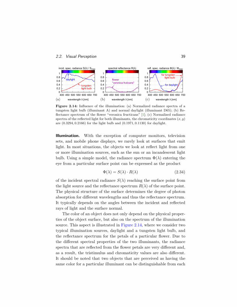
Figure 2.14: Influence of the illumination: (a) Normalized radiance spectra of atungsten light bulb (illuminant A) and normal daylight (illuminant D65); (b) Re-flectance spectrum of the flower “veronica fructicans” [1]; (c) Normalized radiancespectra of the reflected light for both illuminants, the chromaticity coordinates (x, y)are (0.3294, 0.2166) for the light bulb and (0.1971, 0.1130) for daylight.
Illumination. With the exception of computer monitors, televisionsets, and mobile phone displays, we rarely look at surfaces that emitlight. In most situations, the objects we look at reflect light from oneor more illumination sources, such as the sun or an incandescent lightbulb. Using a simple model, the radiance spectrum Φ(λ) entering theeye from a particular surface point can be expressed as the product
Φ(λ) = S(λ) ·R(λ) (2.34)
of the incident spectral radiance S(λ) reaching the surface point fromthe light source and the reflectance spectrum R(λ) of the surface point.The physical structure of the surface determines the degree of photonabsorption for different wavelengths and thus the reflectance spectrum.It typically depends on the angles between the incident and reflectedrays of light and the surface normal.
The color of an object does not only depend on the physical proper-ties of the object surface, but also on the spectrum of the illuminationsource. This aspect is illustrated in Figure 2.14, where we consider twotypical illumination sources, daylight and a tungsten light bulb, andthe reflectance spectrum for the petals of a particular flower. Due tothe different spectral properties of the two illuminants, the radiancespectra that are reflected from the flower petals are very different and,as a result, the tristimulus and chromaticity values are also different.It should be noted that two objects that are perceived as having thesame color for a particular illuminant can be distinguishable from each
40 Acquisition, Representation, Display, and Perception
0
0.5
1
400 450 500 550 600 650 700 750norm
. spe
c. r
adia
nce
wavelength λ [nm]
2856 K (illuminant A)
5000 K8000 K
≈ tungsten light bulb
(a)
0
0.5
1
400 450 500 550 600 650 700 750norm
. spe
c. r
adia
nce
wavelength λ [nm]
morning lightnormal daylight (D65)
twilight (just before dark)
(b)
0
0.1
0.2
0.3
0.4
0.5
0.6
0.7
0.8
0.9
0 0.1 0.2 0.3 0.4 0.5 0.6 0.7 0.8
chro
mat
icity
y
chromaticity x
460470
480
490
500
510
520
530
540
550
560
570
580
590
600
610
620
1000
K2000
K
3000 K
4000 K
5000 K
6000 K
8000 K12000 K∞
E
(c)
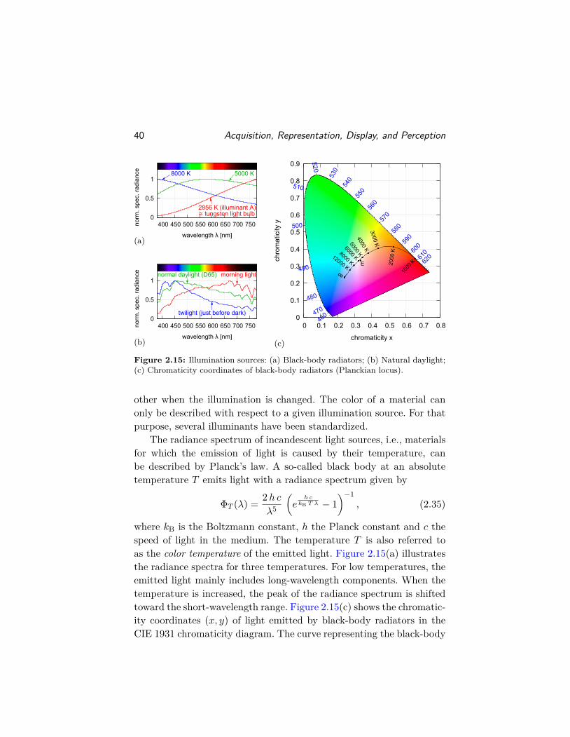
Figure 2.15: Illumination sources: (a) Black-body radiators; (b) Natural daylight;(c) Chromaticity coordinates of black-body radiators (Planckian locus).
other when the illumination is changed. The color of a material canonly be described with respect to a given illumination source. For thatpurpose, several illuminants have been standardized.
The radiance spectrum of incandescent light sources, i.e., materialsfor which the emission of light is caused by their temperature, canbe described by Planck’s law. A so-called black body at an absolutetemperature T emits light with a radiance spectrum given by
ΦT (λ) = 2h cλ5
(e
h ckB T λ − 1
)−1, (2.35)
where kB is the Boltzmann constant, h the Planck constant and c thespeed of light in the medium. The temperature T is also referred toas the color temperature of the emitted light. Figure 2.15(a) illustratesthe radiance spectra for three temperatures. For low temperatures, theemitted light mainly includes long-wavelength components. When thetemperature is increased, the peak of the radiance spectrum is shiftedtoward the short-wavelength range. Figure 2.15(c) shows the chromatic-ity coordinates (x, y) of light emitted by black-body radiators in theCIE 1931 chromaticity diagram. The curve representing the black-body
2.2. Visual Perception 41
radiators for different temperatures is called the Planckian locus. Theradiance spectrum for a black-body radiator of about 2856 K has beenstandardized as illuminant A [42] by the CIE; it represents the typicallight emitted by tungsten filament light bulbs.
There are several light sources, such as fluorescent lamps or light-emitted diodes (LEDs), for which the light emission is not caused bytemperature. The chromaticity coordinates for such illuminants oftendo not lie on the Planckian locus. The light of non-incandescent sourcesis often characterized by the so-called correlated color temperature. Itrepresents the temperature of the black-body radiator for which theperceived color most closely matches that of the considered light source.
With the goal of approximating the radiance spectrum of averagedaylight, the CIE standardized the illuminant D65 [42]. It is based onvarious spectral measurements and has a correlated color temperatureof 6504 K. Daylight for different conditions can be well approximatedby linearly combining three radiance spectra. The CIE specified thesethree radiance spectra and recommended a procedure for determiningthe weights given a correlated color temperature in the range from4000 to 25000 K. These daylight approximations are also referred to asCIE series-D illuminants. Figure 2.15(b) shows the approximations foraverage daylight (illuminant D65), morning light (4300 K) and twilight(12000 K). The chromaticity coordinates of the illuminant D65 specifythe white point of the sRGB format [38]; they are typically also usedas standard setting for the white point of displays.
Chromatic Adaptation. The tristimulus values of light reflected froman objects’ surface highly depend on the spectral composition of thelight source. However, to a large extent, our visual system adapts to thespectral characteristics of the illumination sources. Even though we no-tice the difference between, for example, the orange light of a tungstenlight bulb and the blueish twilight just before dark (see Figure 2.15), asheet of paper is recognized as being white for a large variety of illumi-nation sources. This aspect of the human visual system is referred to aschromatic adaptation. As discussed above, linear color spaces providea mechanism for determining if two light stimuli appear to have the
42 Acquisition, Representation, Display, and Perception
same color, but only under the assumption that the viewing conditionsdo not change. By modeling the chromatic adaptation of the human vi-sual system, we can, to a certain degree, predict how an object observedunder one illuminant looks under a different illuminant.
A simple theory of chromatic adaptation, which was first postulatedby von Kries [88] in 1902, is that the sensitivities of the three conetypes are independently adapted to the spectral characteristics of theillumination sources. With (L1,M1, S1) and (L2,M2, S2) being the coneexcitation responses for two different viewing conditions, the von Kriesmodel can be formulated as L2
M2S2
=
α 0 00 β 00 0 γ
· L1M1S1
. (2.36)
If we assume that the white points, i.e., the LMS tristimulus valuesof light stimuli that appear white, are given by (Lw1,Mw1, Sw1) and(Lw2,Mw2, Sw2) for the two considered viewing conditions, the scalingfactors are determined by
α = Lw2/Lw1, β = Mw2/Mw1, γ = Sw2/Sw1. (2.37)
Today it is known that the chromatic adaptation of our visual sys-tem cannot solely described by an independent re-scaling of the conesensitivity functions, but also includes non-linear components as wellas cognitive effects. Nonetheless, variations of the simple von Kriesmethod are widely used in practice and form the basis of most modernchromatic adaptation models.
A generalized linear model for chromatic adaptation in the CIE 1931XYZ color space can be written as X2
Y2Z2
= M−1CAT ·
α 0 00 β 00 0 γ
·MCAT ·
X1Y1Z1
, (2.38)
where the matrix MCAT specifies the transformation from the XYZcolor space into the color space in which the von Kries-style chromaticadaptation is applied. If the chromaticity coordinates (xw1, yw1) and(xw2, yw2) of the white points for both viewing conditions are given
2.2. Visual Perception 43
and we assume that the relative luminance Y shall not change, thescaling factors can be determined by
α = Aw2/Aw1β = Bw2/Bw1γ = Cw2/Cw1
with
AwkBwkCwk
= M−1CAT ·
xwkywk
11−xwk−ywk
ywk
. (2.39)
The transformation specified by the matrix MCAT is referred to aschromatic adaptation transform. If we strictly follow von Kries’ idea, itspecifies the transformation from the XYZ into the LMS color space.On the basis of several viewing experiments, it has been found thattransformations into color spaces that are represented by so-calledsharpened cone fundamentals yield better results. The chromatic adap-tation transform that is suggested in the color appearance modelCIECAM02 [18, 62] specified by the CIE is given by the matrix
MCAT(CIECAM02) =
0.7328 0.4296 −0.1624−0.7036 1.6974 0.0061
0.0030 −0.0136 0.9834
. (2.40)
For more details about chromatic adaptation transforms and moderncolor appearance models, the reader is referred to [70, 25].
In contrast to the human visual system, digital cameras do not au-tomatically adjust to the properties of the present illumination, theysimply measure the radiance of the light falling through the color filters(see Section 2.4). For obtaining natural looking images, the raw datarecorded by the image sensor have to be processed in order to simulatethe chromatic adaptation of the human visual system. The correspond-ing processing step is referred to as white balancing. It is often basedon a standard chromatic adaptation transform and directly incorpo-rated into the conversion from the internal color space of the camerato the color space of the representation format. With (R1, G1, B1) beingthe recorded tristimulus values and (R2, G2, B2) being the tristimulusvalues of the representation format, we have R2
G2B2
= M−1Rep ·M
−1CAT ·
α 0 00 β 00 0 γ
·MCAT ·MCam ·
R1G1B1
. (2.41)
The matrices MCam and MRep specify the conversion from the cameraand representation RGB spaces, respectively, into the XYZ space. The
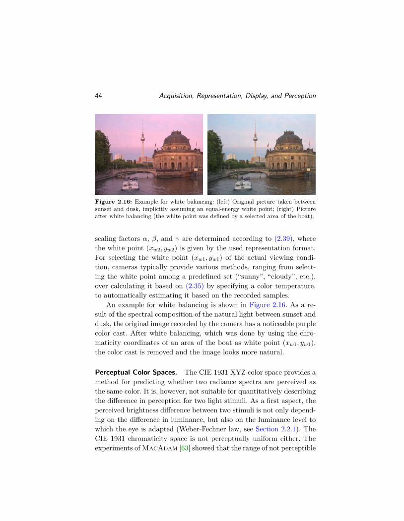
44 Acquisition, Representation, Display, and Perception
Figure 2.16: Example for white balancing: (left) Original picture taken betweensunset and dusk, implicitly assuming an equal-energy white point; (right) Pictureafter white balancing (the white point was defined by a selected area of the boat).
scaling factors α, β, and γ are determined according to (2.39), wherethe white point (xw2, yw2) is given by the used representation format.For selecting the white point (xw1, yw1) of the actual viewing condi-tion, cameras typically provide various methods, ranging from select-ing the white point among a predefined set (“sunny”, “cloudy”, etc.),over calculating it based on (2.35) by specifying a color temperature,to automatically estimating it based on the recorded samples.
An example for white balancing is shown in Figure 2.16. As a re-sult of the spectral composition of the natural light between sunset anddusk, the original image recorded by the camera has a noticeable purplecolor cast. After white balancing, which was done by using the chro-maticity coordinates of an area of the boat as white point (xw1, yw1),the color cast is removed and the image looks more natural.
Perceptual Color Spaces. The CIE 1931 XYZ color space provides amethod for predicting whether two radiance spectra are perceived asthe same color. It is, however, not suitable for quantitatively describingthe difference in perception for two light stimuli. As a first aspect, theperceived brightness difference between two stimuli is not only depend-ing on the difference in luminance, but also on the luminance level towhich the eye is adapted (Weber-Fechner law, see Section 2.2.1). TheCIE 1931 chromaticity space is not perceptually uniform either. Theexperiments of MacAdam [63] showed that the range of not perceptible
2.2. Visual Perception 45
chromaticity differences for a given reference chromaticity (x0, y0) canbe described by an ellipse in the x-y plane centered around (x0, y0), butthe orientation and size of theses so-called MacAdam ellipses8 highlydepend on the considered reference chromaticity (x0, y0).
With the goal of defining approximately perceptual uniform colorspaces with a simple relationship to the CIE 1931 XYZ color space,the CIE specified the color spaces CIE 1976 L∗a∗b∗ [43] and CIE 1976L∗u∗v∗ [44], which are commonly referred to as CIELAB and CIELUV,respectively. Typically, the CIE L∗a∗b∗ color space is considered to moreperceptual uniform. Its relation to the XYZ space is given by L∗
a∗
b∗
=
0 116 0500 −500 0
0 200 −200
· f(X/Xw)f(Y/Yw)f(Z/Zw)
− 16
00
(2.42)
withf(t) =
{3√t : t > ( 6
29)3
13 (29
6 )2 t+ 429 : t ≤ ( 6
29)3 . (2.43)
The values (L∗, a∗, b∗) do not only depend on the considered point inthe XYZ space, but also on the tristimulus values (Xw, Yw, Zw) of thereference white point determined by the present illumination. Hence,the L∗a∗b∗ color space includes a chromatic normalization, which cor-responds to a simple von Kries-style model (2.38) with MCAT equal tothe identity matrix. The function f(t) mimics the non-linear behaviorof the human visual system. The coordinate L∗ is called the lightness,a perceptually corrected version of the relative luminance Y . The com-ponents a∗ and b∗ represents color differences between reddish-magentaand green and yellow and blue, respectively. Hence, the L∗, a∗ and b∗values can be interpreted as non-linear versions of the opponent-colorprocesses discussed in Section 2.2.1.
Due to the approximate perceptual uniformity of the CIE L∗a∗b∗
color space, the difference between two light stimuli can be quantified bythe Euclidean distance between the corresponding (L∗, a∗, b∗) vectors,
∆E =√
(L∗1 − L∗0)2 + (a∗1 − a∗0)2 + (b∗1 − b∗0)2. (2.44)
8MacAdam’s description can be extended to the XYZ space [10, 22], in whichcase the regions of not perceptible color differences are ellipsoids.
46 Acquisition, Representation, Display, and Perception
There are many other color spaces that have been developed fordifferent purposes. Most of them can be derived from the XYZ colorspace, which can be seen as a master color space, since it has beenspecified based on experimental data. For image and video coding, theY’CbCr color space is particularly important. It has some of the proper-ties of CIELAB and will be discussed in Section 2.3, where we describerepresentation formats for image and video coding.
2.2.3 Visual Acuity
The ability of the human visual system to resolve fine details is de-termined by three factors: The resolution of the human optics, thesampling of the projected image by the photoreceptor cells, and theneural processing of the photoreceptor signals. The influence of thefirst two factors was evaluated in several experiments. Measurementsof the modulation transfer function [12, 61, 64] revealed that the humaneye has significant aberrations for large pupil sizes (see Section 2.2.1).At high spatial frequencies, however, large pupil sizes provide an im-proved modulation transfer. The estimated cut-off frequency rangesfrom about 50 cycles per degree (cpd), for pupil sizes of 2 mm, to200 cpd, for pupil sizes of 7.3 mm [61]. In the foveal region, the averagedistance between rows of cones is about 0.5 minutes of arc [92, 21]. Thiscorresponds to a Nyquist frequency of 60 cpd. For the short wavelengthrange of visible light, the image projected on the retina is significantlyblurred due to axial chromatic aberration. The density of the S-conesis also significantly lower than that of M- and L-cones; it correspondsto a Nyquist frequency of about 10 cpd [20].
The impact of the neural processing on the visual acuity can beonly evaluated in connection with the human optics and the retinalsampling. An ophthalmologist checks visual acuity typically using aSnellen chart. At luminance levels of at least 120 cd/m2, a person withnormal visual acuity has to be able to read letters covering a visualangle of 5 minutes of arc, for example, letters of 8.73 mm height ata distance of 6 m. The used letters can be considered to consist ofbasically 3 black and 2 white lines in one direction and, hence, peoplewith normal acuity can resolve spatial frequencies of at least 30 cpd.
2.2. Visual Perception 47
Contrast Sensitivity. The resolving capabilities of the human visualsystem are often characterized by contrast sensitivity functions, whichspecify the contrast threshold between visible and invisible. The con-trast C of a stimulus is typically defined as Michelson contrast
C = Imax − IminImax + Imin
, (2.45)
where Imin and Imax are the minimum and maximum luminance ofthe stimulus. The contrast sensitivity sc = 1/Ct is the reciprocal ofthe contrast Ct at which a pattern is just perceivable. Note that thesmallest possible value of sc = 1 means that, regardless of the contrast,the stimulus is invisible for a human observer.
For analyzing the visual acuity, the contrast sensitivity is typicallymeasured for spatio-temporal sinusoidal stimuli
I(α, t) = I ·(1 + C · cos(2πuα) · cos(2πv t)
), (2.46)
where I = (Imin + Imax)/2 is the average luminance, u is the spatialfrequency in cycles per visual angle, v is the temporal frequency in Hz,α denotes the visual angle, and t represents the time. By varying thespatial and temporal frequency, a function sc(u, v) is obtained, whichis called the spatio-temporal contrast sensitivity function (CSF).
Spatial Contrast Sensitivity. The spatial CSF sc(u) specifies the con-trast sensitivity for sinusoidal stimuli that do not change over time (i.e.,for v = 0). It can be considered a psychovisual version of the modu-lation transfer function. Experimental investigations [87, 13, 91, 86]showed that it highly depends on various parameters, such as the aver-age luminance I and the field of view. A model that well matches the ex-perimental data was proposed by Barten [4]. Figure 2.17(a) illustratesthe basic form of the spatial CSF for foveal vision and different aver-age luminances I. The spatial CSF has a bandpass character. Exceptfor very low luminance levels, the Weber-Fechner law, sc(u) 6= f(I), isvalid in the low frequency range. In the high frequency range, however,the CSF highly depends on the average luminance level I. For photopicluminances, the CSF has its peak sensitivity between 2 and 4 cpd, thecut-off frequency is between 40 and 60 cpd.
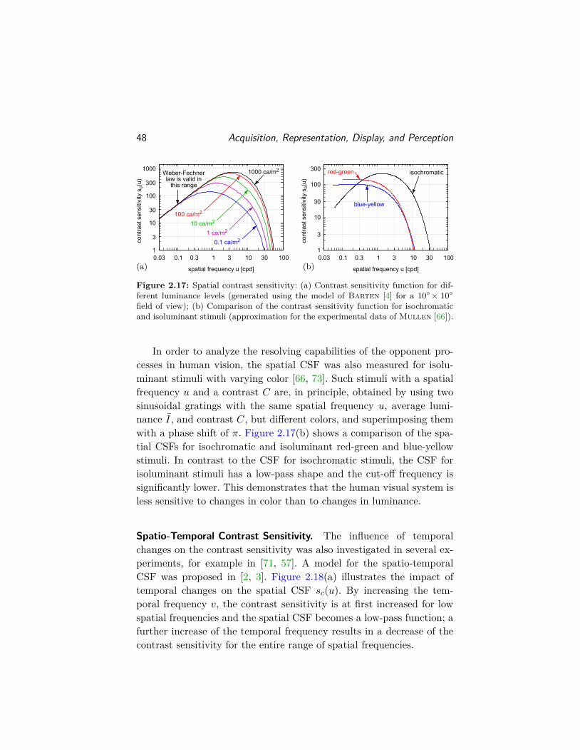
48 Acquisition, Representation, Display, and Perception
3
30
300
1
10
100
1000
0.03 0.3 3 30 0.1 1 10 100
cont
rast
sen
sitiv
ity sc(
u)
spatial frequency u [cpd]
1000 ca/m2
100 ca/m2
10 ca/m2
1 ca/m2
0.1 ca/m2
Weber-Fechnerlaw is valid in
this range
3
30
300
1
10
100
0.03 0.3 3 30 0.1 1 10 100
cont
rast
sen
sitiv
ity sc(
u)
spatial frequency u [cpd]
isochromaticred-green
blue-yellow
(a) (b)
Figure 2.17: Spatial contrast sensitivity: (a) Contrast sensitivity function for dif-ferent luminance levels (generated using the model of Barten [4] for a 10◦× 10◦field of view); (b) Comparison of the contrast sensitivity function for isochromaticand isoluminant stimuli (approximation for the experimental data of Mullen [66]).
In order to analyze the resolving capabilities of the opponent pro-cesses in human vision, the spatial CSF was also measured for isolu-minant stimuli with varying color [66, 73]. Such stimuli with a spatialfrequency u and a contrast C are, in principle, obtained by using twosinusoidal gratings with the same spatial frequency u, average lumi-nance I, and contrast C, but different colors, and superimposing themwith a phase shift of π. Figure 2.17(b) shows a comparison of the spa-tial CSFs for isochromatic and isoluminant red-green and blue-yellowstimuli. In contrast to the CSF for isochromatic stimuli, the CSF forisoluminant stimuli has a low-pass shape and the cut-off frequency issignificantly lower. This demonstrates that the human visual system isless sensitive to changes in color than to changes in luminance.
Spatio-Temporal Contrast Sensitivity. The influence of temporalchanges on the contrast sensitivity was also investigated in several ex-periments, for example in [71, 57]. A model for the spatio-temporalCSF was proposed in [2, 3]. Figure 2.18(a) illustrates the impact oftemporal changes on the spatial CSF sc(u). By increasing the tem-poral frequency v, the contrast sensitivity is at first increased for lowspatial frequencies and the spatial CSF becomes a low-pass function; afurther increase of the temporal frequency results in a decrease of thecontrast sensitivity for the entire range of spatial frequencies.
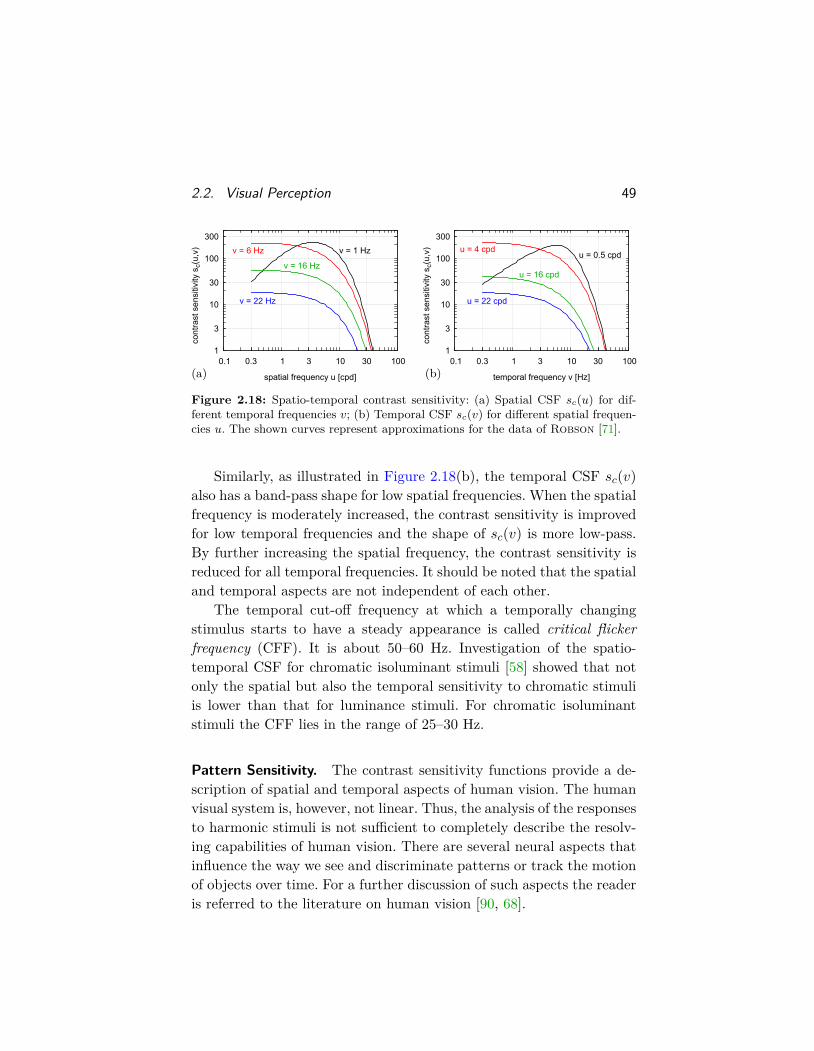
2.2. Visual Perception 49
3
30
300
1
10
100
0.3 3 30 0.1 1 10 100
cont
rast
sen
sitiv
ity sc(
u,v)
spatial frequency u [cpd]
v = 1 Hzv = 6 Hz
v = 16 Hz
v = 22 Hz
3
30
300
1
10
100
0.3 3 30 0.1 1 10 100
cont
rast
sen
sitiv
ity sc(
u,v)
temporal frequency v [Hz]
u = 0.5 cpdu = 4 cpd
u = 16 cpd
u = 22 cpd
(a) (b)
Figure 2.18: Spatio-temporal contrast sensitivity: (a) Spatial CSF sc(u) for dif-ferent temporal frequencies v; (b) Temporal CSF sc(v) for different spatial frequen-cies u. The shown curves represent approximations for the data of Robson [71].
Similarly, as illustrated in Figure 2.18(b), the temporal CSF sc(v)also has a band-pass shape for low spatial frequencies. When the spatialfrequency is moderately increased, the contrast sensitivity is improvedfor low temporal frequencies and the shape of sc(v) is more low-pass.By further increasing the spatial frequency, the contrast sensitivity isreduced for all temporal frequencies. It should be noted that the spatialand temporal aspects are not independent of each other.
The temporal cut-off frequency at which a temporally changingstimulus starts to have a steady appearance is called critical flickerfrequency (CFF). It is about 50–60 Hz. Investigation of the spatio-temporal CSF for chromatic isoluminant stimuli [58] showed that notonly the spatial but also the temporal sensitivity to chromatic stimuliis lower than that for luminance stimuli. For chromatic isoluminantstimuli the CFF lies in the range of 25–30 Hz.
Pattern Sensitivity. The contrast sensitivity functions provide a de-scription of spatial and temporal aspects of human vision. The humanvisual system is, however, not linear. Thus, the analysis of the responsesto harmonic stimuli is not sufficient to completely describe the resolv-ing capabilities of human vision. There are several neural aspects thatinfluence the way we see and discriminate patterns or track the motionof objects over time. For a further discussion of such aspects the readeris referred to the literature on human vision [90, 68].
50 Acquisition, Representation, Display, and Perception
2.3 Representation of Digital Images and Video
In the following, we describe data formats that serve as input formatsfor image and video encoders and as output formats of image and videodecoders. These raw data formats are also referred to as representationformats and specify how visual information is represented as arraysof discrete-amplitude samples. At the sender side of a video commu-nication system, the camera data have to be converted into such arepresentation format and at the receiver side the output of a decoderhas to be correctly interpreted for displaying the transmitted pictures.Important examples for representation formats are the ITU-R Recom-mendations BT.601 [46], BT.709 [46], and BT.2020 [46], which specifyraw data formats for standard definition (SD), high definition (HD),and ultra-high definition (UHD) television, respectively. A discussionof several design aspects for UHD television can be found in [48].
2.3.1 Spatio-Temporal Sampling
In order to process images or videos with a microprocessor or com-puter, the physical quantities describing the visual information haveto be discretized, i.e., they have to be sampled and quantized. Thephysical quantities that we measure in the image plane of a camera areirradiances observed through color filters. Let ccont(x, y, t) be a contin-uous function that represents the irradiance for a particular color filterin the image plane of a camera. In image and video coding applications,orthogonal sampling lattices as illustrated in Figure 2.19(a) are used.The W×H sample array cn[`,m] representing a color component at aparticular time instant tn is, in principle, given by
cn[`,m] = ccont( ` ·∆x, m ·∆y, n ·∆t ) (2.47)
where `, m, and n are integer values with 0≤`<W and 0≤m<H. Thesampling is done by the image sensor of a camera. Due to the finite sizeof the photocells and the finite exposure time, each sample actually rep-resents the integral over approximately a cuboid in the x-y-t space. Thesamples output by an image sensor have discrete amplitudes. However,since the number of provided amplitude levels is significantly greater
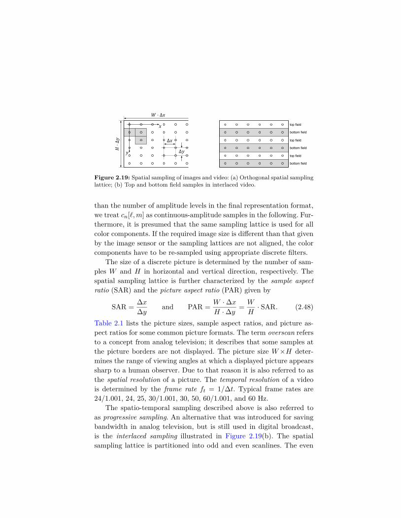
2.3. Representation of Digital Images and Video 51
(a)
∆𝑥
∆𝑦
𝑊 ⋅ ∆𝑥𝐻⋅∆𝑦
𝑥
𝑦
(b)
top field
bottom field
top field
bottom field
top field
bottom field
Figure 2.19: Spatial sampling of images and video: (a) Orthogonal spatial samplinglattice; (b) Top and bottom field samples in interlaced video.
than the number of amplitude levels in the final representation format,we treat cn[`,m] as continuous-amplitude samples in the following. Fur-thermore, it is presumed that the same sampling lattice is used for allcolor components. If the required image size is different than that givenby the image sensor or the sampling lattices are not aligned, the colorcomponents have to be re-sampled using appropriate discrete filters.
The size of a discrete picture is determined by the number of sam-ples W and H in horizontal and vertical direction, respectively. Thespatial sampling lattice is further characterized by the sample aspectratio (SAR) and the picture aspect ratio (PAR) given by
SAR = ∆x∆y and PAR = W ·∆x
H ·∆y = W
H· SAR. (2.48)
Table 2.1 lists the picture sizes, sample aspect ratios, and picture as-pect ratios for some common picture formats. The term overscan refersto a concept from analog television; it describes that some samples atthe picture borders are not displayed. The picture size W×H deter-mines the range of viewing angles at which a displayed picture appearssharp to a human observer. Due to that reason it is also referred to asthe spatial resolution of a picture. The temporal resolution of a videois determined by the frame rate ft = 1/∆t. Typical frame rates are24/1.001, 24, 25, 30/1.001, 30, 50, 60/1.001, and 60 Hz.
The spatio-temporal sampling described above is also referred toas progressive sampling. An alternative that was introduced for savingbandwidth in analog television, but is still used in digital broadcast,is the interlaced sampling illustrated in Figure 2.19(b). The spatialsampling lattice is partitioned into odd and even scanlines. The even

52 Acquisition, Representation, Display, and Perception
Table 2.1: Examples for common picture formats.
picture size sample aspect picture aspect(in samples) ratio (SAR) ratio (PAR)
overscan
720× 576 12:11 4:3 horizontal overscanstandard 720× 480 10:11 4:3 (only 704 samplesdefinition 720× 576 16:11 16:9 are displayed for
720× 480 40:33 16:9 each scanline)
1280× 720 1:1 16:9high
1440× 1080 4:3 16:9 without overscandefinition
1920× 1080 1:1 16:9
ultra-high 3840× 2160 1:1 16:9definition 7680× 4320 1:1 16:9
without overscan
scan lines (starting with index zero) form the top field and the oddscan lines form the bottom field of an interlaced frame. The top andbottom fields are alternatively scanned at successive time instances.The sample arrays of a field have the size W×(H/2). The number offields per second, called the field rate, is twice the frame rate.
2.3.2 Color Representation
For a device-independent description of color information, represen-tation formats often include the specification of linear color spaces.As discussed in Section 2.2.2, displays are not capable of reproducingall colors of the human gamut. And since the number of amplitudelevels required for representing colors with a given accuracy increaseswith increasing gamut, representation formats typically use linear colorspaces with real primaries and non-negative tristimulus values. Thecolor spaces are described by the CIE 1931 chromaticity coordinatesof the primaries and the white point. The 3×3 matrix specifying theconversion between the tristimulus values of the representation formatand the CIE 1931 XYZ color space can be determined by solving thelinear equation system in (2.33). As examples, Figure 2.20 lists thechromaticity coordinates for selected representation formats and illus-trates the gamuts in the chromaticity diagram. In contrast to the HDand UHD specifications BT.709 and BT.2020, the ITU-R Recommen-dation BT.601 for SD television does not include the specification ofa linear color space. For conventional SD television systems, the linear

2.3. Representation of Digital Images and Video 53
SMPTE EBU ITU-R ITU-R170M Tech. 3213 BT.709 BT.2020
xr 0.6300 0.6400 0.6400 0.7080red
yr 0.3400 0.3300 0.3300 0.2920
xg 0.3100 0.2900 0.3000 0.1700green
yg 0.5950 0.6000 0.6000 0.7970
xb 0.1550 0.1500 0.1500 0.1310blue
yb 0.0700 0.0600 0.0600 0.0460
white xw 0.3127 0.3127 0.3127 0.3127(D65) yw 0.3290 0.3290 0.3290 0.3290
D65white
SMPTE 170M(SD 525)
EBU Tech. 3213 (SD 625)
BT.709(HD)
BT.2020 (UHD)
human gamut
x
y
Figure 2.20: Color spaces of selected representation formats: (left) CIE 1931 chro-maticity coordinates for the color primaries and white point; (right) Comparison ofthe corresponding color gamuts to the human gamut.
color spaces specified in EBU Tech. 3213 [24] (for 625-line systems) andSMPTE 170M [77] (for 525-line systems) are used9, which are similar tothat in BT.709. Due to continuing improvements in display technology,the color primaries for UHD specification BT.2020 have been selectedto lie on the spectral locus yielding a significantly larger gamut thanthe SD and HD specifications. As a consequence, BT.2020 also recom-mends larger bit depths for representing amplitude values.
At the sender side, the color sample arrays captured by the imagesensor(s) of the camera have to be converted into the color space of therepresentation format. For each point (`,m) of the sampling lattice, theconversion can be realized by a linear transform according to (2.41)10.If the transform yields a tristimulus vector with one or more negativeentries, the color lies outside the gamut of the representation formatand has to be mapped to a similar color inside the gamut; the easiestway of such a mapping is to set the negative entries equal to zero.It is common sense to scale the transform matrix in a way that thecomponents of the resulting tristimulus vectors have a maximum valueof one. At the receiver side, a similar linear transform is required for
9 Since the 6th edition, BT.601 lists the chromaticity coordinates specified inEBU Tech. 3213 [24] (625-line systems) and SMPTE 170M [77] (525-line systems).
10Note that the white point of the representation format is used for both, thedetermination of the conversion matrix MRep and the calculation of the white bal-ancing factors α, β, and γ. If the camera captures C > 3 color components, theconversion matrix MCam and the combined transform matrix have a size of 3 × C.
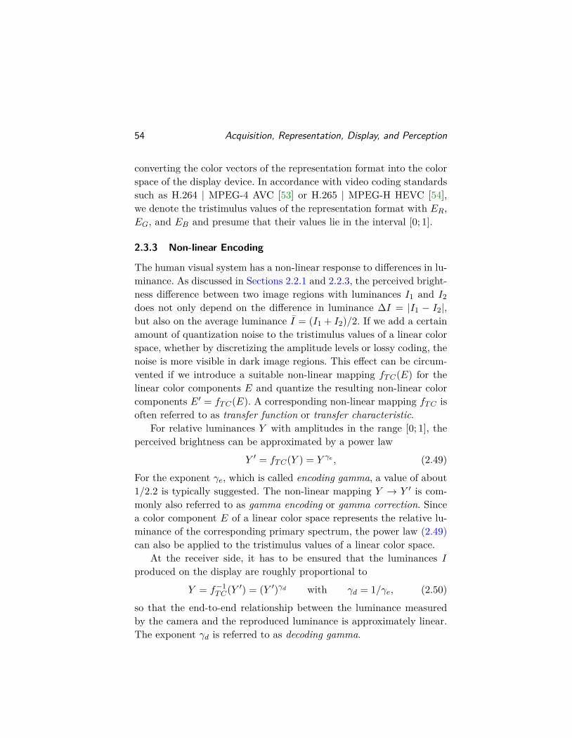
54 Acquisition, Representation, Display, and Perception
converting the color vectors of the representation format into the colorspace of the display device. In accordance with video coding standardssuch as H.264 | MPEG-4 AVC [53] or H.265 | MPEG-H HEVC [54],we denote the tristimulus values of the representation format with ER,EG, and EB and presume that their values lie in the interval [0; 1].
2.3.3 Non-linear Encoding
The human visual system has a non-linear response to differences in lu-minance. As discussed in Sections 2.2.1 and 2.2.3, the perceived bright-ness difference between two image regions with luminances I1 and I2does not only depend on the difference in luminance ∆I = |I1 − I2|,but also on the average luminance I = (I1 + I2)/2. If we add a certainamount of quantization noise to the tristimulus values of a linear colorspace, whether by discretizing the amplitude levels or lossy coding, thenoise is more visible in dark image regions. This effect can be circum-vented if we introduce a suitable non-linear mapping fTC(E) for thelinear color components E and quantize the resulting non-linear colorcomponents E′ = fTC(E). A corresponding non-linear mapping fTC isoften referred to as transfer function or transfer characteristic.
For relative luminances Y with amplitudes in the range [0; 1], theperceived brightness can be approximated by a power law
Y ′ = fTC(Y ) = Y γe , (2.49)
For the exponent γe, which is called encoding gamma, a value of about1/2.2 is typically suggested. The non-linear mapping Y → Y ′ is com-monly also referred to as gamma encoding or gamma correction. Sincea color component E of a linear color space represents the relative lu-minance of the corresponding primary spectrum, the power law (2.49)can also be applied to the tristimulus values of a linear color space.
At the receiver side, it has to be ensured that the luminances Iproduced on the display are roughly proportional to
Y = f−1TC(Y ′) = (Y ′)γd with γd = 1/γe, (2.50)
so that the end-to-end relationship between the luminance measuredby the camera and the reproduced luminance is approximately linear.The exponent γd is referred to as decoding gamma.
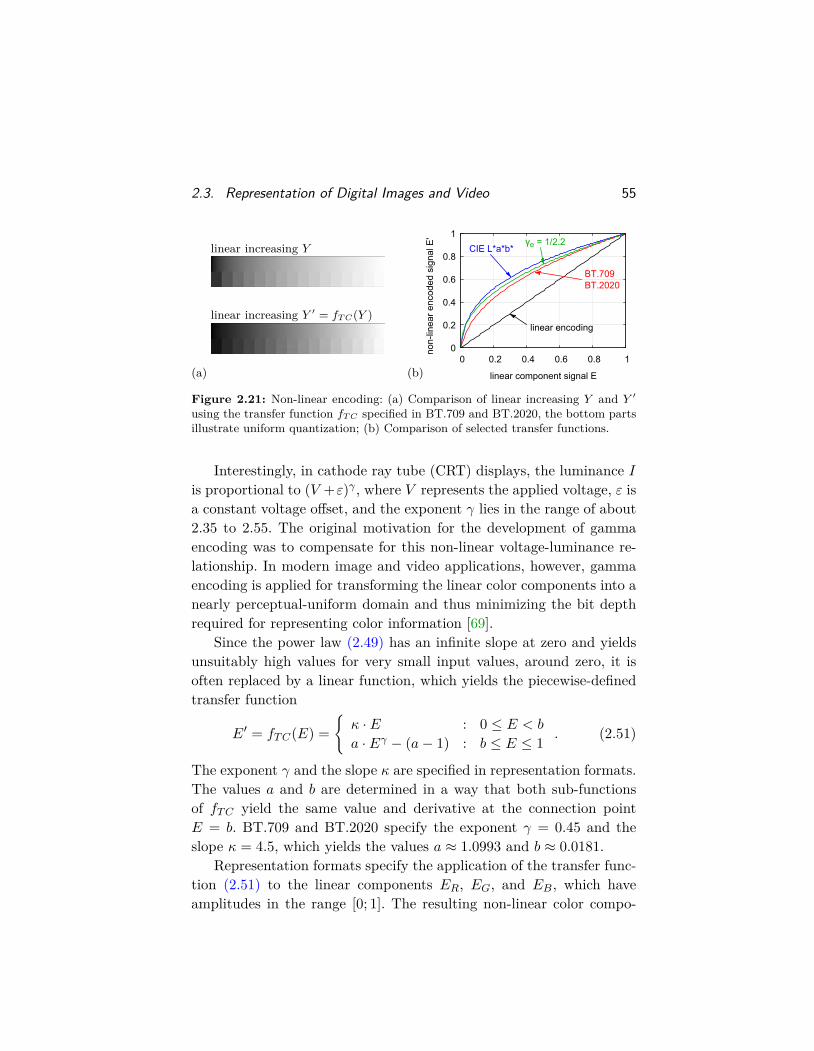
2.3. Representation of Digital Images and Video 55
linear increasing Y
linear increasing Y ′ = fTC(Y )
0
0.2
0.4
0.6
0.8
1
0 0.2 0.4 0.6 0.8 1
non-
linea
r en
code
d si
gnal
E'
linear component signal E
BT.709BT.2020
γe = 1/2.2CIE L*a*b*
linear encoding
(a) (b)
Figure 2.21: Non-linear encoding: (a) Comparison of linear increasing Y and Y ′using the transfer function fTC specified in BT.709 and BT.2020, the bottom partsillustrate uniform quantization; (b) Comparison of selected transfer functions.
Interestingly, in cathode ray tube (CRT) displays, the luminance Iis proportional to (V +ε)γ , where V represents the applied voltage, ε isa constant voltage offset, and the exponent γ lies in the range of about2.35 to 2.55. The original motivation for the development of gammaencoding was to compensate for this non-linear voltage-luminance re-lationship. In modern image and video applications, however, gammaencoding is applied for transforming the linear color components into anearly perceptual-uniform domain and thus minimizing the bit depthrequired for representing color information [69].
Since the power law (2.49) has an infinite slope at zero and yieldsunsuitably high values for very small input values, around zero, it isoften replaced by a linear function, which yields the piecewise-definedtransfer function
E′ = fTC(E) ={κ · E : 0 ≤ E < b
a · Eγ − (a− 1) : b ≤ E ≤ 1 . (2.51)
The exponent γ and the slope κ are specified in representation formats.The values a and b are determined in a way that both sub-functionsof fTC yield the same value and derivative at the connection pointE = b. BT.709 and BT.2020 specify the exponent γ = 0.45 and theslope κ = 4.5, which yields the values a ≈ 1.0993 and b ≈ 0.0181.
Representation formats specify the application of the transfer func-tion (2.51) to the linear components ER, EG, and EB, which haveamplitudes in the range [0; 1]. The resulting non-linear color compo-

56 Acquisition, Representation, Display, and Perception
nents are denoted as E′R, E′G, and E′B; their range of amplitudes isalso [0; 1]. In most applications, ER, EG, and EB have already discreteamplitudes. For a reasonable application of gamma encoding, the bitdepth of the linear components has to be at least 3 bits larger than thebit depth used for representing the gamma-encoded values.
Figure 2.21(a) illustrates the subjective effect of non-linear encodingfor the relative luminance Y of an achromatic signal. In Figure 2.21(b),the transfer function fTC as specified in BT.709 and BT.2020 is com-pared to the simple power law with γe = 1/2.2 and the transfer functionused in the CIE L∗a∗b∗ color space (see Section 2.2.2).
2.3.4 The Y’CbCr Color Representation
Color television was introduced as backwards compatible extension ofthe existing black and white television. This was achieved by trans-mitting two signals with color difference information in addition to theconventional luminance-related signal. As will be discussed in the fol-lowing, the representation of color images as a luminance-related signaland two color difference signals has some advantages due to which it isstill widely used in image and video communication applications.
Firstly, let us assume that the luminance-related signal, which shallbe denoted by L, and the color difference signals C1 and C2 representlinear combinations of the linear color components ER, EG, and EB.The mapping between the vectors (L,C1, C2) and the CIE 1931 XYZcolor space can then be represented by the matrix equation X
YZ
=
Xr Xg Xb
Yr Yg Yb
Zr Zg Zb
· R` Rc1 Rc2
G` Gc1 Gc2
B` Bc1 Bc2
· LC1C2
, (2.52)
where the first matrix specifies the given mapping between the linearRGB color space of the representation format and the XYZ color spaceand the second matrix specifies the mapping from the LC1C2 to theRGB space. We consider the following desirable properties:
• Achromatic signals (x = xw and y = yw) have C1 = C2 = 0;
• Changes in the color difference components C1 or C2 do not haveany impact on the relative luminance Y .

2.3. Representation of Digital Images and Video 57
The first property requires R` = G` = B`. The second criterion isfulfilled if, for k being equal to 1 and 2, we have
Yr ·Rck + Yg ·Gck + Yb ·Bck = 0. (2.53)
Probably to simplify implementations, early researchers chose Rc1 = 0and Bc2 = 0. With s`, sc1 , and sc2 being arbitrary non-zero scalingfactors, this choice yields
L = s` · ( Yr · ER + Yg · EG + Yb · EB )C1 = sc1 · ( −Yr · ER − Yg · EG + (Yr + Yg) · EB )C2 = sc2 · ( (Yg + Yb) · ER − Yg · EG − Yb · EB ).
(2.54)
By using Y = YrER + YgEG + YbEB, we can also write
L = s` · YC1 = sc1 · ( (Yr + Yg + Yb)EB − Y )C2 = sc2 · ( (Yr + Yg + Yb)ER − Y ).
(2.55)
The component L is, as expected, proportional to the relative lumi-nance Y ; the components C1 and C2 represent differences between aprimary component and the appropriately scaled relative luminance Y .
Y’CbCr. Due to decisions made in the early years of color television,the transformation (2.55) from the RGB color space into a color spacewith a luminance-related and two color difference components is appliedafter gamma encoding11. The transformation is given by
E′Y = KR · E′R + (1−KR −KB) · E′B +KB · E′BE′Cb = (E′B − E′Y ) / (2− 2KB)E′Cr = (E′R − E′Y ) / (2− 2KR).
(2.56)
The component E′Y is called the luma component and the color differ-ence signals E′Cb and E′Cr are called chroma components. The terms“luma” and “chroma” have been chosen to indicate that the signals arecomputed as linear combinations of gamma-encoded color components;the non-linear nature is also indicated by the prime symbol. The rep-resentation of color images by a luma and two chroma components is
11In the age of CRT TVs, this processing order had the advantage that the decodedE′R, E′G, and E′B signals could be directly fed to a CRT display.
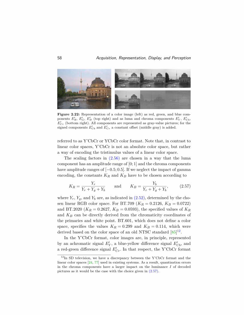
58 Acquisition, Representation, Display, and Perception
Figure 2.22: Representation of a color image (left) as red, green, and blue com-ponents E′R, E′G, E′B (top right) and as luma and chroma components E′Y , E′Cb,E′Cr (bottom right). All components are represented as gray-value pictures; for thesigned components E′Cb and E′Cr a constant offset (middle gray) is added.
referred to as Y’CbCr or YCbCr color format. Note that, in contrast tolinear color spaces, Y’CbCr is not an absolute color space, but rathera way of encoding the tristimulus values of a linear color space.
The scaling factors in (2.56) are chosen in a way that the lumacomponent has an amplitude range of [0; 1] and the chroma componentshave amplitude ranges of [−0.5; 0.5]. If we neglect the impact of gammaencoding, the constants KR and KB have to be chosen according to
KR = YrYr + Yg + Yb
and KB = YbYr + Yg + Yb
, (2.57)
where Yr, Yg, and Yb are, as indicated in (2.52), determined by the cho-sen linear RGB color space. For BT.709 (KR = 0.2126, KB = 0.0722)and BT.2020 (KR = 0.2627, KB = 0.0593), the specified values of KR
and KB can be directly derived from the chromaticity coordinates ofthe primaries and white point. BT.601, which does not define a colorspace, specifies the values KR = 0.299 and KB = 0.114, which werederived based on the color space of an old NTSC standard [85]12.
In the Y’CbCr format, color images are, in principle, representedby an achromatic signal E′Y , a blue-yellow difference signal E′Cb, anda red-green difference signal E′Cr. In that respect, the Y’CbCr format
12In SD television, we have a discrepancy between the Y’CbCr format and thelinear color spaces [24, 77] used in existing systems. As a result, quantization errorsin the chroma components have a larger impact on the luminance I of decodedpictures as it would be the case with the choice given in (2.57).
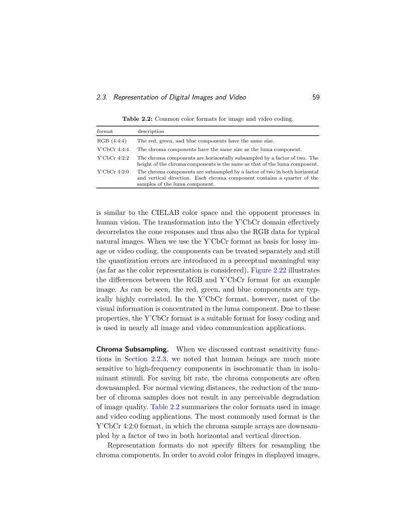
2.3. Representation of Digital Images and Video 59
Table 2.2: Common color formats for image and video coding.
format description
RGB (4:4:4) The red, green, and blue components have the same size.
Y’CbCr 4:4:4 The chroma components have the same size as the luma component.
Y’CbCr 4:2:2 The chroma components are horizontally subsampled by a factor of two. Theheight of the chroma components is the same as that of the luma component.
Y’CbCr 4:2:0 The chroma components are subsampled by a factor of two in both horizontaland vertical direction. Each chroma component contains a quarter of thesamples of the luma component.
is similar to the CIELAB color space and the opponent processes inhuman vision. The transformation into the Y’CbCr domain effectivelydecorrelates the cone responses and thus also the RGB data for typicalnatural images. When we use the Y’CbCr format as basis for lossy im-age or video coding, the components can be treated separately and stillthe quantization errors are introduced in a perceptual meaningful way(as far as the color representation is considered). Figure 2.22 illustratesthe differences between the RGB and Y’CbCr format for an exampleimage. As can be seen, the red, green, and blue components are typ-ically highly correlated. In the Y’CbCr format, however, most of thevisual information is concentrated in the luma component. Due to theseproperties, the Y’CbCr format is a suitable format for lossy coding andis used in nearly all image and video communication applications.
Chroma Subsampling. When we discussed contrast sensitivity func-tions in Section 2.2.3, we noted that human beings are much moresensitive to high-frequency components in isochromatic than in isolu-minant stimuli. For saving bit rate, the chroma components are oftendownsampled. For normal viewing distances, the reduction of the num-ber of chroma samples does not result in any perceivable degradationof image quality. Table 2.2 summarizes the color formats used in imageand video coding applications. The most commonly used format is theY’CbCr 4:2:0 format, in which the chroma sample arrays are downsam-pled by a factor of two in both horizontal and vertical direction.
Representation formats do not specify filters for resampling thechroma components. In order to avoid color fringes in displayed images,

60 Acquisition, Representation, Display, and Perception
4:4:4 4:2:0 (BT.2020)4:2:2 4:2:0 (MPEG-1) 4:2:0 (MPEG-2)
Figure 2.23: Nominal locations of chroma samples (indicated by circles) relative tothat of luma samples (indicated by crosses) for different chroma sampling formats.
the phase shifts of the filters and thus the locations of the chroma sam-ples relative to the luma samples should be known. For 4:4:4 and 4:2:2sampling formats, representation formats and video coding standardsgenerally specify that the top-left chroma samples coincide with thetop-left luma sample (see Figure 2.23). For the 4:2:0 format, however,different alternatives are used. While BT.2020 specifies that the top-leftchroma samples coincide with the top-left luma sample (third picturein Figure 2.23), in the video coding standards MPEG-1 Video [45],H.261 [49], and H.263 [50], the chroma samples are located in the cen-ter of the four associated luma samples (fourth picture in Figure 2.23).And in the video coding standards H.262 | MPEG-2 Video [52], H.264 |MPEG-4 AVC [53], and H.265 | MPEG-H HEVC [54], the nominaloffset between the top-left chroma and luma samples is zero in hor-izontal and half a luma sample in vertical direction (fifth picture inFigure 2.23). Video coding standards such as H.264 | MPEG-4 AVCand H.265 | MPEG-H HEVC include syntax that allows to indicate thelocation of chroma samples in the 4:2:0 format inside the bitstream.
Constant Luminance Y’CbCr. The application of gamma encodingbefore calculating the Y’CbCr components in (2.56) has the effect thatchanges in the chroma components due to quantization or subsamplinginfluence the relative luminance of the displayed signal. BT.2020 [47]specifies an alternative format, which is given by the components
E′Y C = fTC (KR · ER + (1−KR −KB) · EG +KB · EB ) (2.58)E′CbC = (E′B − E′Y C) /NB (2.59)E′CrC = (E′R − E′Y C) /NR. (2.60)

2.3. Representation of Digital Images and Video 61
The sign-dependent scaling factors NB and NR are
NX ={
2a (1−KγX) : E′X − E′Y C ≤ 0
2a (1− (1−KX)γ)− 1 : E′X − E′Y C > 0 , (2.61)
where a and γ represent the corresponding parameters of the transferfunction fTC in (2.51). By defining sY = Yr + Yg + Yb and using (2.58)we obtain for the relative luminance Y of the decoded signal
Y = sY · (KRER + (1−KR −KB)EG +KB EB)= sY ·
(KRER +
(f−1TC(E′Y C)−KRER −KB EB
)+KB EB
)= sY · f−1
TC(E′Y C). (2.62)
The relative luminance Y depends only on E′Y C . Due to that reasonthe alternative format is also referred to as constant luminance Y’CbCrformat. In the document BT.2246 [48], the impact on video coding wasevaluated by encoding eight test sequences, given in an RGB format,with H.265 | MPEG-H HEVC [54]. The reconstruction quality wasmeasured in the CIELAB color space using the distortion measure ∆Egiven in (2.44). It is reported that by choosing the constant luminanceformat instead of the conventional Y’CbCr format, on average 12% bitrate savings are obtained for the same average distortion. The con-stant luminance Y’CbCr format has similar properties as the currentlydominating standard Y’CbCr format and could replace it in image andvideo applications without requiring any adjustments despite the mod-ified transformation from and to the linear RGB color space.
2.3.5 Quantization of Sample Values
Finally, for obtaining discrete-amplitude samples suitable for codingand digital transmission, the luma and chroma components E′Y , E′Cb,and E′Cr are quantized using uniform quantization. The ITU-R Recom-mendations BT.601, BT.709, and BT.2020 specify that the correspond-ing integer color components Y , Cb, and Cr are obtained according to
Y =[
(219 · E′Y + 16) · 2B−8], (2.63)
Cb =[
(224 · E′Cb + 128) · 2B−8], (2.64)
Cr =[
(224 · E′Cr + 128) · 2B−8], (2.65)
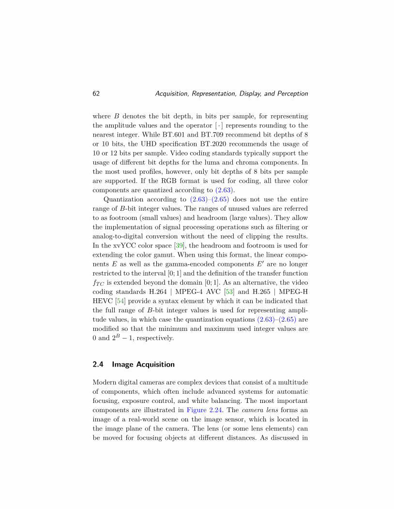
62 Acquisition, Representation, Display, and Perception
where B denotes the bit depth, in bits per sample, for representingthe amplitude values and the operator [ · ] represents rounding to thenearest integer. While BT.601 and BT.709 recommend bit depths of 8or 10 bits, the UHD specification BT.2020 recommends the usage of10 or 12 bits per sample. Video coding standards typically support theusage of different bit depths for the luma and chroma components. Inthe most used profiles, however, only bit depths of 8 bits per sampleare supported. If the RGB format is used for coding, all three colorcomponents are quantized according to (2.63).
Quantization according to (2.63)–(2.65) does not use the entirerange of B-bit integer values. The ranges of unused values are referredto as footroom (small values) and headroom (large values). They allowthe implementation of signal processing operations such as filtering oranalog-to-digital conversion without the need of clipping the results.In the xvYCC color space [39], the headroom and footroom is used forextending the color gamut. When using this format, the linear compo-nents E as well as the gamma-encoded components E′ are no longerrestricted to the interval [0; 1] and the definition of the transfer functionfTC is extended beyond the domain [0; 1]. As an alternative, the videocoding standards H.264 | MPEG-4 AVC [53] and H.265 | MPEG-HHEVC [54] provide a syntax element by which it can be indicated thatthe full range of B-bit integer values is used for representing ampli-tude values, in which case the quantization equations (2.63)–(2.65) aremodified so that the minimum and maximum used integer values are0 and 2B − 1, respectively.
2.4 Image Acquisition
Modern digital cameras are complex devices that consist of a multitudeof components, which often include advanced systems for automaticfocusing, exposure control, and white balancing. The most importantcomponents are illustrated in Figure 2.24. The camera lens forms animage of a real-world scene on the image sensor, which is located inthe image plane of the camera. The lens (or some lens elements) canbe moved for focusing objects at different distances. As discussed in
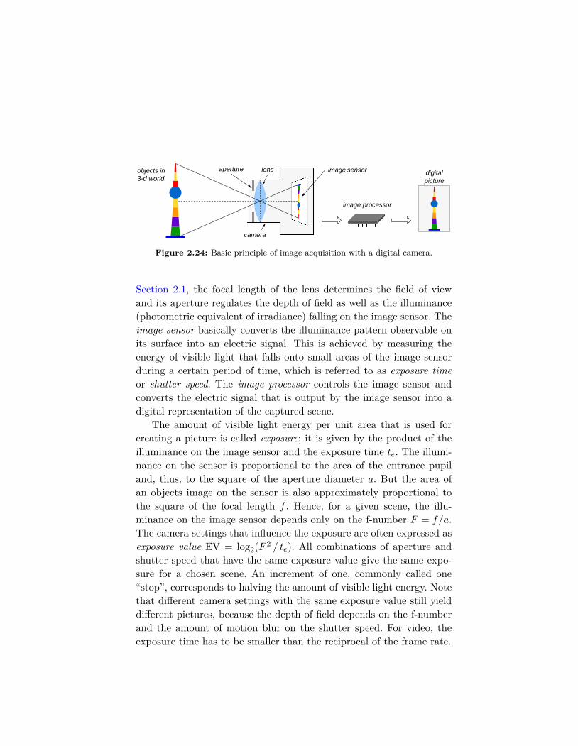
2.4. Image Acquisition 63
objects in
3-d world
camera
lens image sensor aperture
image processor
digital
picture
Figure 2.24: Basic principle of image acquisition with a digital camera.
Section 2.1, the focal length of the lens determines the field of viewand its aperture regulates the depth of field as well as the illuminance(photometric equivalent of irradiance) falling on the image sensor. Theimage sensor basically converts the illuminance pattern observable onits surface into an electric signal. This is achieved by measuring theenergy of visible light that falls onto small areas of the image sensorduring a certain period of time, which is referred to as exposure timeor shutter speed. The image processor controls the image sensor andconverts the electric signal that is output by the image sensor into adigital representation of the captured scene.
The amount of visible light energy per unit area that is used forcreating a picture is called exposure; it is given by the product of theilluminance on the image sensor and the exposure time te. The illumi-nance on the sensor is proportional to the area of the entrance pupiland, thus, to the square of the aperture diameter a. But the area ofan objects image on the sensor is also approximately proportional tothe square of the focal length f . Hence, for a given scene, the illu-minance on the image sensor depends only on the f-number F = f/a.The camera settings that influence the exposure are often expressed asexposure value EV = log2(F 2 / te). All combinations of aperture andshutter speed that have the same exposure value give the same expo-sure for a chosen scene. An increment of one, commonly called one“stop”, corresponds to halving the amount of visible light energy. Notethat different camera settings with the same exposure value still yielddifferent pictures, because the depth of field depends on the f-numberand the amount of motion blur on the shutter speed. For video, theexposure time has to be smaller than the reciprocal of the frame rate.
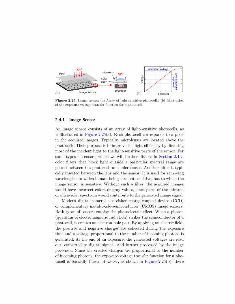
64 Acquisition, Representation, Display, and Perception
photocell
microlens
image sensor
color
filter
light filter
light
volta
ge
exposure
saturation voltage
satu
ratio
nex
posu
re le
vel
(a) (b)
Figure 2.25: Image sensor: (a) Array of light-sensitive photocells; (b) Illustrationof the exposure-voltage transfer function for a photocell.
2.4.1 Image Sensor
An image sensor consists of an array of light-sensitive photocells, asis illustrated in Figure 2.25(a). Each photocell corresponds to a pixelin the acquired images. Typically, microlenses are located above thephotocells. Their purpose is to improve the light efficiency by directingmost of the incident light to the light-sensitive parts of the sensor. Forsome types of sensors, which we will further discuss in Section 2.4.2,color filters that block light outside a particular spectral range areplaced between the photocells and microlenses. Another filter is typi-cally inserted between the lens and the sensor. It is used for removingwavelengths to which human beings are not sensitive, but to which theimage sensor is sensitive. Without such a filter, the acquired imageswould have incorrect colors or gray values, since parts of the infraredor ultraviolet spectrum would contribute to the generated image signal.
Modern digital cameras use either charge-coupled device (CCD)or complementary metal-oxide-semiconductor (CMOS) image sensors.Both types of sensors employ the photoelectric effect. When a photon(quantum of electromagnetic radiation) strikes the semiconductor of aphotocell, it creates an electron-hole pair. By applying an electric field,the positive and negative charges are collected during the exposuretime and a voltage proportional to the number of incoming photons isgenerated. At the end of an exposure, the generated voltages are readout, converted to digital signals, and further processed by the imageprocessor. Since the created charges are proportional to the numberof incoming photons, the exposure-voltage transfer function for a pho-tocell is basically linear. However, as shown in Figure 2.25(b), there

2.4. Image Acquisition 65
is a saturation level, which is determined by the maximum collectiblecharge. If the exposure exceeds the saturation level for a significantamount of photocells, the captured image is overexposed; the lost im-age details cannot be recovered by the following signal processing.
Sensor Noise. The number of photons that arrive at a particular pho-tocell during the exposure time is random; it can be well modeled asrandom variable with a Poisson distribution. The resulting noise in thecaptured image is called photon shot noise. The Poisson distributionhas the property that the variance σ2 is equal to the mean µ. Hence, ifwe assume a linear relationship between the number of photons and thegenerated voltage, the signal-to-noise ratio (SNR) of the output signal isproportional to the average number of incoming photons (µ2/σ2 = µ).Other types of noise that affect the image quality are:
• Dark current noise: A certain amount of charges per time unitcan be also created by thermal vibration;• Read noise: Thermal noise in readout circuitry;• Reset noise: Some charges may remain after resetting the photo-cells at the beginning of an exposure;• Fixed pattern noise: Caused by manufacturing variations acrossthe photocells of a sensor.
Most noise sources are independent of the irradiance on the sensor. Anexception is the photon shot noise, which becomes predominant abovea certain irradiance level. The SNR of a captured image increases withthe number of photons arriving at a photocell during exposure. Con-sequently, pictures and videos captured with the small image sensors(and small photocells) of smartphones are considerably noisier thanthose captured with the large sensors of professional cameras.
ISO Speed. The ISO speed or ISO sensitivity is a measure that wasoriginally standardized by the International Organization for Standard-ization (ISO) for specifying the light-sensitivity of photographic films.It is now also used as a measure for the sensitivity of image sensors.Digital cameras typically allow to select the ISO speed inside a given
66 Acquisition, Representation, Display, and Perception
range. Changing the ISO speed modifies the amplification factor of thesensors output signal before analog-to-digital conversion. The ISO sys-tem defines a linear and a logarithmic scale. Digital cameras typicallyuse the linear scale (with values of 100, 200, etc.), for which a doublingof the ISO sensitivity corresponds to a doubling of the amplificationfactor. Note that higher ISO values correspond to lower signal-to-noiseratios, since the noise in the sensors output is also amplified.
The ISO speed is the third parameter, beside the aperture and theshutter speed, by which the exposure of a picture can be controlled.Typically, an image is considered to be correctly exposed if nearly theentire range of digital amplitude levels is utilized and the portion ofsaturated photocells or clipped sample values is very small. For a givenscene, the photographer or videographer can select one of multiple suit-able combinations of aperture, shutter speed, and ISO sensitivity and,thus, control the depth of field, motion blur, and noise level withincertain ranges. For filming in dark environments, increasing the ISOsensitivity is often the only way to achieve the required frame rate.
2.4.2 Capture of Color Images
The photocells of an image sensor basically only count photons. Theycannot discriminate between photons of different wavelengths insidethe visible spectrum. As discussed in Section 2.2.2, we need however atleast three image signals, each for a different range of wavelengths, forrepresenting color images. Consequently, the spectrum of visible lighthas to be decomposed into three spectral components. There are twodominating techniques in today’s cameras: Three-sensor systems andsingle sensors with color filter arrays. A third technique, the multi-layersensor, is also used in some cameras.
Three-Sensor Systems. As the name suggests, three-sensor systemsuse three image sensors, each for a different part of the spectrum. Thelight that falls through the lens is split by a trichroic prism assembly,which consists of two prisms with dichroic coatings (dichroic prisms),and is illustrated in Figure 2.26(a). The dichroic optical coatings havethe property that they reflect or transmit light depending on the lights
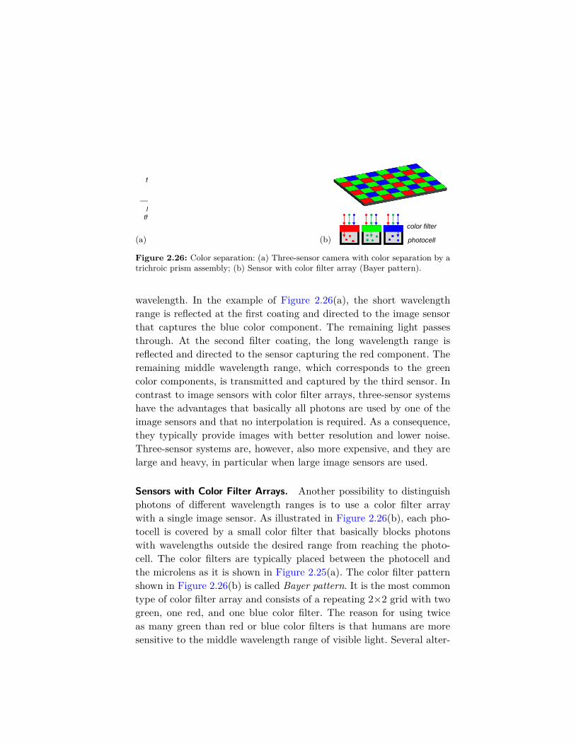
2.4. Image Acquisition 67
image sensor
(red component)
image sensor
(blue component)
image sensor
(green component)
filter coatingfilter coating
light falling
through lens
color filter
photocell(a) (b)
Figure 2.26: Color separation: (a) Three-sensor camera with color separation by atrichroic prism assembly; (b) Sensor with color filter array (Bayer pattern).
wavelength. In the example of Figure 2.26(a), the short wavelengthrange is reflected at the first coating and directed to the image sensorthat captures the blue color component. The remaining light passesthrough. At the second filter coating, the long wavelength range isreflected and directed to the sensor capturing the red component. Theremaining middle wavelength range, which corresponds to the greencolor components, is transmitted and captured by the third sensor. Incontrast to image sensors with color filter arrays, three-sensor systemshave the advantages that basically all photons are used by one of theimage sensors and that no interpolation is required. As a consequence,they typically provide images with better resolution and lower noise.Three-sensor systems are, however, also more expensive, and they arelarge and heavy, in particular when large image sensors are used.
Sensors with Color Filter Arrays. Another possibility to distinguishphotons of different wavelength ranges is to use a color filter arraywith a single image sensor. As illustrated in Figure 2.26(b), each pho-tocell is covered by a small color filter that basically blocks photonswith wavelengths outside the desired range from reaching the photo-cell. The color filters are typically placed between the photocell andthe microlens as it is shown in Figure 2.25(a). The color filter patternshown in Figure 2.26(b) is called Bayer pattern. It is the most commontype of color filter array and consists of a repeating 2×2 grid with twogreen, one red, and one blue color filter. The reason for using twiceas many green than red or blue color filters is that humans are moresensitive to the middle wavelength range of visible light. Several alter-
68 Acquisition, Representation, Display, and Perception
natives to the Bayer pattern are used by some manufacturers. Thesepatterns either use filters of different colors or a different arrangement,or they include filters with a fourth color.
Since each photocell of a sensor can only count photons for one ofthe wavelength ranges, the sample arrays for the color components con-tain a significant number of holes. The unknown sample values haveto be generated using interpolation algorithms. This processing stepis commonly called demosaicing. For a Bayer sensor, actually half ofthe samples for the green component and three quarters of the sam-ples for the red and blue components have to be generated. If theassumptions underlying the employed demosaicing algorithm are nottrue for an image region, interpolation errors can cause visible artifacts.The most frequently observed artifacts are Moiré patterns, which typi-cally appear as wrong color patterns in fine detailed image regions. Forreducing demosaicing artifacts, digital image sensors with color filterarrays typically incorporate an optical low-pass filter or anti-aliasingfilter, which is placed directly in front of the sensor. Often, this filterconsists of two layers of a birefringent material and is combined withan infrared absorption filter. The optical low-pass filter splits every rayof light into four rays, each of which falls on one photocell of a 2×2cluster. By decreasing the high-frequency components of the irradiancepattern on the photocell array, it reduces the demosaicing artifacts,but also the sharpness of the captured image. Image sensors with colorfilter arrays are smaller, lighter, and less expensive than three-sensorsystems. But due to the color filters they have a lower light efficiency.The demosaicing can cause visible interpolation artifacts; in connectionwith the often applied optical filtering it also reduces the sharpness.
Multi-Layer Image Sensors. In a multi-layer sensor, the photocellsfor different wavelength ranges are not arranged in a two-dimensional,but a three-dimensional array. At each spatial location, three photodi-odes are vertically stacked. The sensor employs the property that theabsorption coefficient of silicon is highly wavelength dependent. As aresult, each of the three stacked photodiodes at a sample location re-sponds to a different wavelength range. The sample values of the three
2.4. Image Acquisition 69
primary colors (red, green, blue) are generated by processing the cap-tured signals. Since three color samples are captured for each spatiallocation, optical low-pass filtering and demosaicing is not required andinterpolation artifacts do not occur. The spectral sensitivity curves re-sulting from the employed wavelength separation by absorption are lesslinearly related to the cone fundamentals than typical color filters. Asa consequence, it is often reported that multi-layer sensors have a lowercolor accuracy than sensors with color filter arrays.
2.4.3 Image Processor
The signals that are output by the image sensor have to be furtherprocessed and eventually converted into a format suitable for imageor video exchange. As a first step, which is required for any furthersignal processing, the analog voltage signals have to be converted intodigital signals. In order to reduce the impact of this quantization onthe following processing, typically a bit depth significantly larger thanthe bit depth of the final representation format is used. The analog-to-digital conversion is sometimes integrated into the sensor.
For converting the obtained digital sensor signals into a representa-tion format, the following processing steps are required: Demosaicing(for sensors with color filter arrays, Section 2.4.2), a conversion fromthe camera color space to the linear color space of the representationformat, including white balancing (Section 2.2.2), gamma encoding ofthe linear color components (Section 2.3.3), optionally, a transformfrom the linear color space to a Y’CbCr format (Section 2.3.4), anda final quantization of the sample values (Section 2.3.5). Beside theserequired processing steps, image processors often also apply algorithmsfor improving the image quality, for example, denoising and sharpeningalgorithms or processing steps for reducing the impact of lens imperfec-tions, such as vignetting, geometrical distortions, and chromatic aber-rations, in the output images. Particularly in consumer cameras, theraw image data are typically also compressed using an image or videoencoder. The outputs of the camera are then bitstreams that conformto a widely accepted coding standard, such as JPEG [51] or H.264 |MPEG-4 AVC [53], and are embedded in a container format.

70 Acquisition, Representation, Display, and Perception
2.5 Display of Images and Video
In most applications, we capture and encode visual information foreventually presenting them to human beings. Display devices act as in-terface between machine and human. At the present time, a rather largevariety of display techniques are available. New technologies and im-provements to existing technologies are still developed. Independent ofthe actual used technology, for producing the sensation of color, eachelement of a displayed picture has to be composed of at least threeprimary colors (see Section 2.2.2). The actual employed technology de-termines the chromaticity coordinates of the primary colors and, thus,the display-internal color space. In general, samples of the representa-tion format provided to the display device have to be transformed intothe display color representation; this transformation typically includesgamma decoding and a color space conversion. Modern display devicesoften apply additional signal processing algorithms for improving theperceived quality of natural video. In the following, we briefly reviewsome important display techniques. For a more detailed discussion, thereader is referred to the overview in [70].
Cathode Ray Tube (CRT) Displays. Some decades ago, all devicesfor displaying natural pictures were cathode ray tube (CRT) displays.It is the oldest type of electronic display technology, but has now beennearly completely replaced by more modern technologies. As illustratedin Figure 2.27(a), a CRT display basically consists of electron guns, adeflection system, and a phosphor-coated screen. Each electron guncontains a heated cathode that produces electrons by thermionic emis-sion. By applying electric fields the electrons are accelerated and fo-cused to form an electron beam. When the electron beam hits thephosphor-coated screen, it causes the emission of photons. The inten-sity of the emitted light is controlled by varying the electric field inthe electron gun. For producing a picture on the screen, the electronbeam is linewise swept over the screen, typically 50 or 60 times per sec-ond. The direction of the beam is controlled by the deflection systemconsisting of magnetic coils. In color CRT displays, three electron gunsand three types of phosphors, each for emitting photons for one of the

2.5. Display of Images and Video 71
electron
beams
shadow
mask
screen with
phosphors
electron
guns deflection system
(magnetic coils)
screen
backlight
V
polarizer liquid
crystals color
filters polarizer
(a) (b)
cell with red
phosphor
cell with green
phosphor
cell with blue
phosphor
+ - + - + - + - + - + - + - + + + +
+ + - - - -
- - - +
emission of
red light
emission of
green light
emission of
blue light (c) (d)
Figure 2.27: Basic principles of display technologies: (a) Cathode ray tube (CRT)display; (b) Liquid crystal display (LCD); (c) Plasma display; (d) OLED display.
primary colors red, green, and blue, are used. The different phosphorsare arranged in clusters or stripes. A shadow masks mounted in frontof the screen prevents electrons from hitting the wrong phosphor.
Liquid Crystal Displays (LCDs). Liquid crystals used in displays areliquid organic substances with a crystal molecular structure. They arearranged in a layer between two transparent electrodes in a way thatthe alignment of the liquid crystals inside the layer can be controlledby the applied voltage. LCDs employ the effect that depending onthe orientation of the liquid crystals inside the layer and, thus, theapplied voltage, the polarization direction of the transmitted light ismodified. The basic structure of LCDs is illustrated in Figure 2.27(b).The light emitted by the displays backlight is passed through a firstpolarizer, which is followed by the liquid crystal layer and a secondpolarizer with a polarization direction perpendicular to that of the firstpolarizer. By adjusting the voltages applied to the liquid crystal layer,the modification of the polarization direction and, thus, the amount of

72 Acquisition, Representation, Display, and Perception
light transmitted through the second polarizer is controlled. Finally, thelight is passed through a layer with color filters (typically red, green,and blue filters) and a color picture perceivable by human beings isgenerated on the surface of the screen. A disadvantage of LCDs is thata backlight is required and a significant amount of light is absorbed.Due to that reason, LCDs have a rather large power consumption anddo not achieve such a good black level as plasma or OLED displays.
Plasma Displays. Plasma displays are based on the phenomenon ofgas discharge. As illustrated in Figure 2.27(c), a layer of cells typicallyfilled with a mixture of helium and xenon [70] is embedded betweentwo electrodes. The electrode at the front side of the display has to betransparent. When a voltage is applied to a cell, the accelerated elec-trons may ionize the contained gas for a short duration. If the excitedatoms return to their ground state, photons with a wavelength insidethe ultraviolet (UV) range are emitted. A part of the UV photons ex-cites the phosphors inside the cell, which eventually emit light in thevisible range. The intensity of the emitted light can be controlled by theapplied voltage. For obtaining color images, three types of phosphors,which emit light in the red, green, and blue range of the spectrum, areused. The corresponding cells are arranged in a suitable spatial layout.
OLED Displays. Organic light-emitting diode (OLED) displays are arelatively new technology. OLEDs consist of organic substances thatemit visible light when an electric current is passed through them. Alayer of organic semiconductor is situated between two electrodes, seeFigure 2.27(d). At least one of the electrodes is transparent. If a voltageis applied, the electrons and holes injected from the cathode and anode,respectively, form electron-hole pairs called excitons. When an excitonrecombines, the excess energy is emitted in the form of a photon; thisprocess is called radiative recombination. The wavelength of the emittedphoton depends on the band energy of the organic material. The lightintensity can be controlled by adjusting the applied voltage. In OLEDdisplays, typically three types of OLEDs with organic substances thatemit light in the red, green, and blue wavelength range are used.

2.6. Chapter Summary 73
Projectors. In contrast to the display devices discussed so far, projec-tors, also commonly called beamers, do not display the final image onthe light modulator itself, but on a diffusely reflecting screen. Due tothe loose coupling of the light modulator and screen, very large imagescan be displayed. That is why projectors are particularly suitable forlarge audiences. There are three dominant projection techniques: LCDprojectors, DLP projectors, and LCoS projectors.
In LCD projectors, the white light of a bright lamp is first split intored, green, and blue components, either by dichroic mirrors or prisms(see Section 2.4.2). Each of the resulting beams is passed through a sep-arate transparent LCD panel, which modulates the intensity accordingto the sample values of the corresponding color component. Finally, themodulated beams are combined by dichroic prisms and passed througha lens, which projects the image on the screen.
Digital light processing (DLP) projectors use a chip with micro-scopic mirrors, one for each pixel. The mirrors can be rotated to sendlight from a lamp either through the lens or towards a light absorber. Byquickly toggling the mirrors, the intensity of the light falling throughthe lens can be modulated. Color images are typically generated byplacing a color wheel between the lamp and the micromirror chip, sothat the color components of an image are sequentially displayed.
Liquid crystal on silicon (LCoS) projectors are similar to LCD pro-jectors, but instead of transparent LCD panels, they use reflective lightmodulators (similar to DLP projectors). The light modulators basicallyconsist of a liquid crystal layer that is fabricated directly on top of asilicon chip. The silicon is coated with a highly reflective metal, whichsimultaneously acts as electrode and mirror. As in LCD panels, the lightmodulation is achieved by changing the orientation of liquid crystals.
2.6 Chapter Summary
In this section, we gave an overview of some fundamental properties ofimage formation and human visual perception, and based on certainaspects of human vision, we reviewed the basic principles that are usedfor capturing, representing, and displaying digital video signals.
74 Acquisition, Representation, Display, and Perception
For acquiring video signals, the lens of a camera projects a sceneof the three-dimensional world onto the surface of an image sensor.The focal length and aperture of the lens determine the field of viewand the depth of field of the projection. Independent of the fabricationquality of the lens, the resolution of the image on the sensor is limited bydiffraction; its effect increases with decreasing aperture. For real lenses,the image quality is additionally reduced by optical aberrations such asgeometric distortions, spherical aberrations, or chromatic aberrations.
The human visual system has similar components as a camera; alens projects an image onto the retina, where the image is sampled bylight-sensitive cells. The photoreceptor responses are send to the brain,where the visual information is interpreted. Under well-lit conditions,three types of photoreceptor cells with different spectral sensitivities areactive. They basically map the infinite-dimensional space of electromag-netic spectra onto a three-dimensional space. Hence, light stimuli withdifferent spectra can be perceived as having the same color. This prop-erty of human vision is the basis of all color reproduction techniques; itis employed in capturing, representing, and displaying image and videosignals. For defining a common color system, the CIE standardizeda so-called standard colorimetric observer by defining color-matchingfunctions based on experimental data. The derived CIE 1931 XYZ colorspace represents the basis for specifying color in video communicationapplications. In display devices, colors are typically reproduced by mix-ing three suitably selected primary lights; it is, however, not possibleto reproduce all colors perceivable by humans. Color spaces that arespanned by three primaries are called linear color spaces. The humaneye adapts to the illumination of a scene; this aspect has to be takeninto account when processing the signals acquired with an image sen-sor. The acuity of human vision is determined by several factors suchas the optics of the eye, the density of photoreceptor cells, and theneural processing. Human beings are more sensitive to details in theluminance than to details in the quality of color.
Certain properties of human vision are also exploited for efficientlyrepresenting visual information. For describing color information, eachvideo picture consists of three samples arrays. The primary colors are

2.6. Chapter Summary 75
specified in the CIE 1931 XYZ color space. Since the human visualsystem has a non-linear response to differences in luminance, the linearcolor components are non-linear encoded. This processing step, alsocalled gamma encoding, yields color components with the propertythat a certain amount of quantization noise has approximately the samesubjective impact on dark and light image regions. In most video codingapplications, the gamma-encoded color components are transformedinto a Y’CbCr format, in which color pictures are specified using aluminance-related component, called luma component, and two colordifference components, which are called chroma components. By thistransformation, the color components are effectively decorrelated. Sincehumans are significantly more sensitive to details in luminance than todetails in color difference data, the chroma components are typicallydownsampled. In the most common format, the Y’CbCr 4:2:0 format,the chroma components contain only a quarter of the samples of theluma component. The luma and chroma sample values are typicallyrepresented with a bit depth of 8 or 10 bits per sample.
The image sensor in a camera samples the illuminance pattern thatis projected onto its surface and converts it into a discrete representa-tion of a picture. Each cell of an image sensor corresponds to an imagepoint and basically counts the photons arriving during the exposuretime. For capturing color images, the incident light has to be split intoat least three spectral ranges. In most digital cameras, this is achievedeither by using a trichroic beam splitter with a separate image sensorfor each color component or by mounting a color filter array on top of asingle image sensor. In display devices, color images are reproduced bymixing (at least) three primary colors for each image point accordingto the corresponding sample values. Important display technologies areCRT, LCD, plasma, and OLED displays. For large audiences, as in acinema, projection technologies are typically used.
References
[1] Sarah E. J. Arnold, Samia Faruq, Vincent Savolainen, Peter W. McOwan,and Lars Chittka. FReD: The Floral Reflectance Database – A Web Por-tal for Analyses of Flower Colour. PLoS ONE, 5(12):e14287, December2010. http://reflectance.co.uk.
[2] Peter G. J. Barten. Spatiotemporal model for the contrast sensitivity ofthe human eye and its temporal aspects. In Jan P. Allebach and Ber-nice E. Rogowitz, editors, Proc. SPIE, Human Vision, Visual Processing,and Digital Display IV, volume 1913. SPIE, September 1993.
[3] Peter G. J. Barten. Contrast Sensitivity of the Human Eye and Its Ef-fects on Image Quality. SPIE Optical Engineering Press, Bellinghan,Washington, 1999.
[4] Peter G. J. Barten. Formula for the contrast sensitivity of the humaneye. In Yoichi Miyake and D. Rene Rasmussen, editors, Proc. SPIE,Image Quality and System Performance, volume 5294, pages 231–238.SPIE, December 2003.
[5] D. A. Baylor, B. J. Nunn, and J. L. Schnapf. Spectral sensitivity ofcones of the monkey macaca fascicularis. The Journal of Physiology,390(1):145–160, 1987.
[6] Max Born and Emil Wolf. Principles of Optics: Electromagnetic The-ory of Propagation, Interference and Diffraction of Light. CambridgeUniversity Press, Cambridge, UK, 7th (expanded) edition, 1999.
76
References 77
[7] D. H. Brainard and A. Stockman. Colorimetry. In M. Bass, C. DeCusatis,J. Enoch, V. Lakshminarayanan, G. Li, C. Macdonald, V. Mahajan, andE. van Stryland, editors, Vision and Vision Optics, volume III of The Op-tical Society of America Handbook of Optics, pages 10.1–10.56. McGrawHill, 3rd edition, 2009.
[8] Arthur D. Broadbent. A critical review of the development of theCIE1931 RGB color-matching functions. Color Research & Application,29(4):267–272, August 2004.
[9] P. K. Brown and G. Wald. Visual pigments in single rods and cones ofthe human retina. Science, 144(3614):45–52, April 1964.
[10] W. R. T. Brown and D. L. MacAdam. Visual sensitivities to combinedchromaticity and luminance differences. Journal of the Optical Societyof America, 39(10):808–823, 1949.
[11] G. Buchsbaum and A. Gottschalk. Trichromacy, opponent colours codingand optimum colour information transmission in the retina. Proceedingsof the Royal Society B: Biological Sciences, 220(1218):89–113, November1983.
[12] F. W. Campbell and R. W. Gubisch. Optical quality of the human eye.The Journal of Physiology, 186(3):558–578, 1966.
[13] F. W. Campbell and J. G. Robson. Application of Fourier analysis to thevisibility of gratings. The Journal of Physiology, 197(3):551–566, 1968.
[14] CIE. CIE Proceedings 1924. Cambridge University Press, Cambridge,1926.
[15] CIE. CIE Proceedings 1931. Cambridge University Press, Cambridge,1932.
[16] CIE. CIE Proceedings 1951. Bureau Central de la CIE, Paris, 1951.[17] CIE. CIE Proceedings 1963. Bureau Central de la CIE, Paris, 1964.[18] CIE. A Colour Appearance Model for Colour Management Systems:
CIECAM02, Publication 159:2004. Bureau Central de la CIE, Vienna,2004.
[19] CIE. Fundamental Chromaticity Diagram with Physiological Axes –Part 1, Publication 170-1. Bureau Central de la CIE, Vienna, 2006.
[20] Christine A. Curcio, Kimberly A. Allen, Kenneth R. Sloan, Connie L.Lerea, James B. Hurley, Ingrid B. Klock, and Ann H. Milam. Distributionand morphology of human cone photoreceptors stained with anti-blueopsin. The Journal of Comparative Neurology, 312(4):610–624, October1991.
78 References
[21] Christine A. Curcio, Kenneth R. Sloan, Robert E. Kalina, and Anita E.Hendrickson. Human photoreceptor topography. The Journal of Com-parative Neurology, 292(4):497–523, February 1990. Data available athttp://www.cis.uab.edu/curcio/PRtopo.
[22] H. R. Davidson. Calculation of color differences from visual sensitivityellipsoids. Journal of the Optical Society of America, 41(12):1052–1055,1951.
[23] Russell L. De Valois, Isreal Abramov, and Gerald H. Jacobs. Analysisof response patterns of LGN cells. Journal of the Optical Society ofAmerica, 56(7):966–977, July 1966.
[24] European Broadcasting Union. EBU standard for chromaticity tolerancesfor studio monitors. EBU Tech. 3213, August 1975.
[25] Mark D. Fairchild. Color Appearance Models. John Wiley & Sons, 3rdedition, 2013.
[26] Hugh S. Fairman, Michael H. Brill, and Henry Hemmendinger. How theCIE 1931 color-matching functions were derived fromWright-Guild data.Color Research & Application, 22(1):11–23, February 1997.
[27] K. S. Gibson and E. P. T. Tyndall. Visibility of radiant energy. ScientificPapers of the Bureau of Standards, 19(475):131–191, 1923.
[28] Joseph W. Goodman. Introduction to Fourier Optics. The MacGraw-HillCompanies, Inc., 1996.
[29] H. Grassmann. Zur Theorie der Farbenmischung. Annalen der Physik,165(5):69–84, 1853.
[30] H. Gross, F. Blechinger, and B. Achtner. Survey of Optical Instruments,volume 4 of Handbook of Optical Instruments. Wiley-VCH Verlag GmbH& Co. KGaA, Weinheim, 2008.
[31] J. Guild. A trichromatic colorimeter suitable for standardisation work.Transactions of the Optical Society, 27(2):106–129, December 1925.
[32] J. Guild. The colorimetric properties of the spectrum. PhilosophicalTransactions of the Royal Society A: Mathematical, Physical and Engi-neering Sciences, 230(681-693):149–187, January 1932.
[33] Eugene Hecht. Optics. Addison-Wesley, 4th edition, 2001.[34] H. Helmholtz. Handbuch der Physiologischen Optik, volume IX of Allge-
meine Encyklopädie der Physik. Leopold Voss, Leipzig, 1867.[35] Ewald Hering. Grundzüge der Lehre vom Lichtsinn. Verlag von Julius
Springer, Berlin, 1920.
References 79
[36] H. Hofer. Organization of the human trichromatic cone mosaic. Journalof Neuroscience, 25(42):9669–9679, October 2005.
[37] Leo M. Hurvich and Dorothea Jameson. Some quantitative aspects of anopponent-colors theory. II. brightness, saturation, and hue in normal anddichromatic vision. Journal of the Optical Society of America, 45(8):602–616, August 1955.
[38] IEC. Multimedia systems and equipment – Colour measurement andmanagement – Part 2-1: Colour management – Default RGB colour space– sRGB. International Standard 61966-2-1, October 1999.
[39] IEC. Extended-gamut YCC colour space for video applications – xvYCC.IEC 61966-2-4, January 2006.
[40] Institute of Ophthalmology, University College London. Colour & VisionResearch laboratory and database. http://www.cvrl.org.
[41] ISO and CIE. Colorimetry – Part 1: CIE standard colorimetric observers.ISO/IEC 11664-1 | CIE S 014-1, 2007.
[42] ISO and CIE. Colorimetry – Part 2: CIE standard illuminants. ISO/IEC11664-2 | CIE S 014-2, 2007.
[43] ISO and CIE. Colorimetry – Part 4: CIE 1976 L*a*b* colour space.ISO/IEC 11664-4 | CIE S 014-4, 2008.
[44] ISO and CIE. Colorimetry – Part 5: CIE 1976 L*u*v* colour space andu’, v’ uniform chromaticity scale diagram. ISO/IEC 11664-5 | CIE S014-5, 2009.
[45] ISO/IEC. Coding of moving pictures and associated audio for digitalstorage media at up to 1.5 Mbit/s – part 2: Video. ISO/IEC 11172-2,1993.
[46] ITU-R. Studio encoding parameters of digital television for standard 4:3and wide-screen 16:9 aspect ratios. Recommendation ITU-R BT.601-7,March 2011.
[47] ITU-R. Parameter values for ultra-high definition television systems forproduction and international programme exchange. RecommendationITU-R BT.2020-1, June 2014.
[48] ITU-R. The present state of ultra-high definition television. ReportITU-R BT.2246-3, March 2014.
[49] ITU-T. Video codec for audiovisual services at p × 64 kbits. ITU-TRecommendation H.261, edition 3, March 1993.
[50] ITU-T. Video coding for low bit rate communication. ITU-T Recom-mendation H.263, edition 3, January 2005.
80 References
[51] ITU-T and ISO/IEC. Digital compression and coding of continuous-tonestill images – requirements and guidelines. ITU-T Recommendation T.81| ISO/IEC 10918-1, September 1992.
[52] ITU-T and ISO/IEC. Generic coding of moving pictures and associatedaudio information: Video. ITU-T Recommendation H.262 | ISO/IEC13818-2, edition 2, February 2000.
[53] ITU-T and ISO/IEC. Advanced video coding for generic audiovisualservices. ITU-T Recommendation H.264 | ISO/IEC 14496-10, edition 8,April 2013.
[54] ITU-T and ISO/IEC. High efficiency video coding. ITU-T Recommen-dation H.265 | ISO/IEC 23008-10, edition 1, April 2013.
[55] Dorothea Jameson and Leo M. Hurvich. Some quantitative aspects of anopponent-colors theory. I. chromatic responses and spectral saturation.Journal of the Optical Society of America, 45(7):546–552, July 1955.
[56] D. B. Judd. Report of U.S. Secretariat Committee on Colorimetry andArtificial Daylight. In Proceedings of the Twelfth Session of the CIE,volume 1, part 7, Stockholm, 1951. Bureau Central de la CIE, Paris.
[57] D. H. Kelly. Frequency doubling in visual responses. Journal of theOptical Society of America, 56(11):1628–1632, 1966.
[58] D. H. Kelly. Spatiotemporal variation of chromatic and achromatic con-trast thresholds. Journal of the Optical Society of America, 73(6):742–749, 1983.
[59] G. Kirchhoff. Zur Theorie der Lichtstrahlen. Annalen der Physik,254(4):663–695, 1883.
[60] Jan J. Koenderink. Color for the Sciences. MIT Press, Cambridge, MA,2010.
[61] Junzhong Liang and David R. Williams. Aberrations and retinal im-age quality of the normal human eye. Journal of the Optical Society ofAmerica A, 14(11):2873–2883, November 1997.
[62] Ming Ronnier Luo and Changjun Li. CIECAM02 and its recent develop-ments. In Christine Fernandez-Maloigne, editor, Advanced Color ImageProcessing and Analysis, pages 19–58. Springer New York, May 2012.
[63] David L. MacAdam. Visual sensitivities to color differences in daylight.Journal of the Optical Society of America, 32(5):247–273, 1942.
[64] Susana Marcos. Image quality of the human eye. International Ophthal-mology Clinics, 43(2):43–62, 2003.
References 81
[65] James Clerk Maxwell. Experiments on colour, as perceived by the eye,with remarks on colour-blindness. Transactions of the Royal Society ofEdinburgh, 21(02):275–298, January 1857.
[66] Kathy T. Mullen. The contrast sensitivity of human colour vision to red-green and blue-yellow chromatic gratings. The Journal of Physiology,359:381–400, February 1985.
[67] G. A. Østerberg. Topography of the layer of rods and cones in the humanretina. Acta Ophthalmologica, 13(Supplement 6):1–97, 1935.
[68] Stephen E. Palmer. Vision Science: Photons to Phenomenology. A Brad-ford Book. MIT Press, Cambridge, MA, 1999.
[69] Charles Poynton. Digital Video and HDTV Algorithms and Interfaces.The Morgan Kaufmann Series in Computer Graphics and GeometricModeling. Morgan Kaufmann Publishers, San Francisco, CA, 2003.
[70] Erik Reinhard, Erum Arif Khan, Ahmet Oguz Akyüz, and Garrett M.Johnson. Color Imaging: Fundamentals and Applications. A K Peters,Ltd., Wellesley, MA, 2008.
[71] J. G. Robson. Spatial and temporal contrast-sensitivity functions of thevisual system. Journal of the Optical Society of America, 56(8):1141–1142, August 1966.
[72] J. L. Schnapf, T. W. Kraft, and D. A. Baylor. Spectral sensitivity ofhuman cone photoreceptors. Nature, 325(6103):439–441, January 1987.
[73] Nobutoshi Sekiguchi, David R. Williams, and David H. Brainard.Aberration-free measurements of the visibility of isoluminant gratings.Journal of the Optical Society of America A, 10(10):2105–2117, 1993.
[74] L. T. Sharpe, A. Stockman, W. Jagla, and H. Jägle. A luminous efficiencyfunction, V ∗(λ), for daylight adaptation. Journal of Vision, 5(11):948–968, December 2005.
[75] Lindsay T. Sharpe, Andrew Stockman, Wolfgang Jagla, and Herbert Jä-gle. A luminous efficiency function, V ∗
D65(λ), for daylight adaptation: Acorrection. Color Research & Application, 36(1):42–46, February 2011.
[76] T. Smith and J. Guild. The C.I.E. colorimetric standards and their use.Transactions of the Optical Society, 33(3):73–134, January 1932.
[77] SMPTE. Composite analog video signal — NTSC for studio applications.SMPTE Standard 170M-2004, November 2004.
[78] A. Sommerfeld. Mathematische Theorie der Diffraction. MathematischeAnnalen, 47(2–3):317–374, June 1896.
82 References
[79] W. S. Stiles and J. M. Burch. N.P.L. colour-matching investigation: Finalreport (1958). Optica Acta: International Journal of Optics, 6(1):1–26,January 1959.
[80] A. Stockman and D. H. Brainard. Color vision mechanism. In M. Bass,C. DeCusatis, J. Enoch, V. Lakshminarayanan, G. Li, C. Macdonald,V. Mahajan, and E. van Stryland, editors, Vision and Vision Optics,volume III of The Optical Society of America Handbook of Optics, pages11.1–11.86. McGraw Hill, 3rd edition, 2009.
[81] Andrew Stockman and Lindsay T. Sharpe. The spectral sensitivities ofthe middle- and long-wavelength-sensitive cones derived from measure-ments in observers of known genotype. Vision Research, 40(13):1711–1737, June 2000.
[82] Andrew Stockman, Lindsay T. Sharpe, and Clemens Fach. The spectralsensitivity of the human short-wavelength sensitive cones derived fromthresholds and color matches. Vision Research, 39(17):2901–2927, August1999.
[83] G. Svaetichin. Spectral response curves from single cones. Acta Physio-logica Scandinavica, 39(Supplement 134):17–46, 1956.
[84] Gunnar Svaetichin and Edward F. MacNichol. Retinal mechanisms forchromatic and achromatic vision. Annals of the New York Academy ofSciences, 74(2):385–404, November 1958.
[85] United States National Television System Committee. Recommendationfor transmission standards for color television, December 1953.
[86] A. van Meeteren and J. J. Vos. Resolution and contrast sensitivity atlow luminances. Vision Research, 12(5):825–833, May 1972.
[87] Floris L. van Nes and Maarten A. Bouman. Spatial modulation transferin the human eye. Journal of the Optical Society of America, 57(3):401–406, March 1967.
[88] Johannes von Kries. Theoretische Studien über die Umstimmung desSehorgans. In Festschrift der Albrecht-Ludwigs-Universität in Freiburg,pages 143–158. C. A. Wagner’s Universitäts-Buchdruckerei, Freiburg,Germany, 1920.
[89] J. J. Vos. Colorimetric and photometric properties of a 2◦ fundamentalobserver. Color Research & Application, 3(3):125–128, July 1978.
[90] Brian A. Wandell. Foundations of Vision. Sinauer Associates, Inc., Sun-derland, Massachusetts, 1995.

References 83
[91] A. Watanabe, T. Mori, S. Nagata, and K. Hiwatashi. Spatial sine-waveresponses of the human visual system. Vision Research, 8(9):1245–1263,September 1968.
[92] David R. Williams. Topography of the foveal cone mosaic in the livinghuman eye. Vision Research, 28(3):433–454, 1988.
[93] W. D. Wright. A trichromatic colorimeter with spectral primaries. Trans-actions of the Optical Society, 29(5):225–242, May 1928.
[94] W. D. Wright. A re-determination of the trichromatic coefficients ofthe spectral colours. Transactions of the Optical Society, 30(4):141–164,March 1929.
[95] G. Wyszecki and W. S. Stiles. Color Science: Concepts and Methods,Quantitative Data and Formulae. John Wiley & Sons, Inc., New York,2nd edition, 1982.
[96] T. Young. The Bakerian Lecture: On the theory of light and colours.Philosophical Transactions of the Royal Society of London, 92(0):12–48,January 1802.