20

Part B: Sample Design Procedures for the SACMEQ II Project This part of the chapter has described the sample design procedures that were employed for the SACMEQ II Project. First, a detailed description has been presented of the step-by-step procedures involved in the design of the samples, the selection of the samples, and the construction of sampling weights. Second, information has been presented on the “evaluation” of the SACMEQ II sampling procedures - in terms of the calculation of response rates, design effects, effective sample sizes, and standard errors of sampling.

Some Constraints on Sample Design Sample designs in the field of education are usually prepared amid a network of competing constraints. These designs need to adhere to established survey sampling theory and, at the same time, give due recognition to the financial, administrative, and socio-political settings in which they are to be applied. The “best” sample design for a particular project is one that provides levels of sampling accuracy that are acceptable in terms of the main aims of the project, while simultaneously limiting cost, logistic, and procedural demands to manageable levels. The major constraints that were established prior to the preparation of the sample designs for the SACMEQ II Project have been listed below. Target Population: The target population definitions should focus on Grade 6 pupils attending registered mainstream government or non-government schools. In addition, the defined target population should be constructed by excluding no more than 5 percent of pupils from the desired target population. Bias Control: The sampling should conform to the accepted rules of scientific probability sampling. That is, the members of the defined target population should have a known and non-zero probability of selection into the sample so that any potential for bias in sample estimates due to variations from “epsem sampling” (equal probability of selection method) may be addressed through the use of appropriate sampling weights (Kish, 1965). Sampling Errors: The sample estimates for the main criterion variables should conform to the sampling accuracy requirements set down by the International Association for the Evaluation of Educational Achievement (Ross, 1991). That is, the standard error of sampling for the pupil tests should be of a magnitude that is equal to, or smaller than, what would be achieved by employing a simple random sample of 400 pupils (Ross, 1985). Response Rates: Each SACMEQ country should aim to achieve an overall response rate for pupils of 80 percent. This figure was based on the wish to achieve or exceed a response rate of 90 percent for schools and a response rate of 90 percent for pupils within schools. Administrative and Financial Costs: The number of schools selected in each country should recognize limitations in the administrative and financial resources available for data collection. Other Constraints: The number of pupils selected to participate in the data collection in each selected school should be set at a level that will maximize validity of the within-school data collection for the pupil reading and mathematics tests.

21

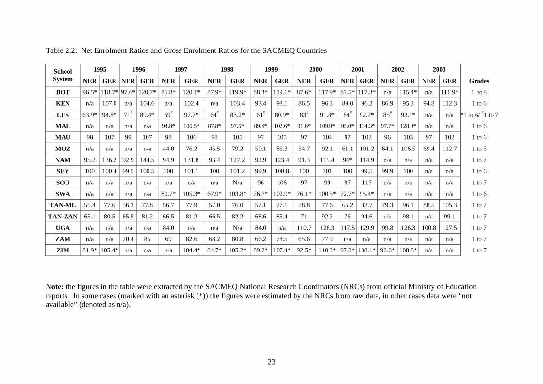
The Specification of the Target Population The target population for both the SACMEQ I and SACMEQ II Projects was focussed on the Grade 6 level for three main reasons. First, Grade 6 identified a point near the end of primary schooling where school participation rates were reasonably high for most of the seven countries that participated in the SACMEQ I data collection during 1995-1997, and also reasonably high for most of the fourteen countries that participated in the SACMEQ II collection during 2000-2002. For this reason, Grade 6 represented a point that was suitable for making an assessment of the contribution of primary schooling towards the literacy and numeracy levels of a broad cross-section of society. (Note: The Net and Gross Enrolment Ratios for the period 1995 to 2003 have been presented for the SACMEQ countries in Table 2.2. The NRCs used official statistical reports to prepare these values. In some Ministries these data were collected and collated in a format that permitted the construction of ratios for either Grades 1-6 or Grades 1-7. In other countries it was necessary for the National Research Coordinator to calculate the ratios from available raw data. In Uganda some of the estimated Net Enrolment Ratios were greater than 100 – a result that was theoretically not possible and probably arose from inaccuracies in estimating the numbers of pupils in the relevant age cohort between Population Censuses). Second, the NRCs considered that testing pupils at grade levels lower than Grade 6 was problematic – because in some SACMEQ countries the lower grades were too close to the transition point between the use of local and national languages by teachers in the classroom. This transition point generally occurred at around Grade 3 level – but in some rural areas of some countries it was thought to be as high as Grade 4 level. Third, the NRCs were of the opinion that the collection of home background information from pupils at grade levels lower than Grade 6 was likely to lack validity for certain key “explanatory” variables. For example, the NRCs felt that children at lower grade levels did not know how many years of education that their parents had received, and they also had difficulty in accurately describing the socioeconomic environment of their own homes (for example, the number of books at home). (a) Desired Target Population The desired target population definition for the SACMEQ II Project was exactly the same (except for the year) as was employed for the SACMEQ I Project. This consistency was maintained in order to be able to make valid cross-national and cross-time estimates of “change” in the conditions of schooling and the quality of education. The desired target population definition for the SACMEQ II Project was as follows. “All pupils at Grade 6 level in 2000 (at the first week of the eighth month of the school year) who were attending registered mainstream primary schools.” Note that the year dates for this definition were varied for two countries (Mauritius in 2001, and Malawi in 2002) in order to coincide with delayed data collections.

23

Table 2.2: Net Enrolment Ratios and Gross Enrolment Ratios for the SACMEQ Countries

School System

1995 1996 1997 1998 1999 2000 2001 2002 2003 NER GER NER GER NER GER NER GER NER GER NER GER NER GER NER GER NER GER Grades

BOT 96.5* 118.7* 97.6* 120.7* 85.8* 120.1* 87.9* 119.9* 88.3* 119.1* 87.6* 117.9* 87.5* 117.3* n/a 115.4* n/a 111.9* 1 to 6

KEN n/a 107.0 n/a 104.6 n/a 102.4 n/a 103.4 93.4 98.1 86.5 96.3 89.0 96.2 86.9 95.3 94.8 112.3 1 to 6

LES 63.9* 94.8* 71# 89.4* 69# 97.7* 64# 83.2* 61# 80.9* 83# 91.8* 84# 92.7* 85# 93.1* n/a n/a *1 to 6/ #1 to 7

MAL n/a n/a n/a n/a 94.8* 106.5* 87.8* 97.5* 89.4* 102.6* 91.6* 109.9* 95.0* 114.3* 97.7* 128.0* n/a n/a 1 to 6

MAU 98 107 99 107 98 106 98 105 97 105 97 104 97 103 96 103 97 102 1 to 6

MOZ n/a n/a n/a n/a 44.0 76.2 45.5 79.2 50.1 85.3 54.7 92.1 61.1 101.2 64.1 106.5 69.4 112.7 1 to 5

NAM 95.2 136.2 92.9 144.5 94.9 131.8 93.4 127.2 92.9 123.4 91.3 119.4 94* 114.9 n/a n/a n/a n/a 1 to 7

SEY 100 100.4 99.5 100.5 100 101.1 100 101.2 99.9 100.8 100 101 100 99.5 99.9 100 n/a n/a 1 to 6

SOU n/a n/a n/a n/a n/a n/a n/a N/a 96 106 97 99 97 117 n/a n/a n/a n/a 1 to 7

SWA n/a n/a n/a n/a 80.7* 105.3* 67.9* 103.8* 76.7* 102.9* 76.1* 100.5* 72.7* 95.4* n/a n/a n/a n/a 1 to 6

TAN-ML 55.4 77.6 56.3 77.8 56.7 77.9 57.0 76.0 57.1 77.1 58.8 77.6 65.2 82.7 79.3 96.1 88.5 105.3 1 to 7

TAN-ZAN 65.1 80.5 65.5 81.2 66.5 81.2 66.5 82.2 68.6 85.4 71 92.2 76 94.6 n/a 98.1 n/a 99.1 1 to 7

UGA n/a n/a n/a n/a 84.0 n/a n/a N/a 84.0 n/a 110.7 128.3 117.5 129.9 99.8 126.3 100.8 127.5 1 to 7

ZAM n/a n/a 70.4 85 69 82.6 68.2 80.8 66.2 78.5 65.6 77.9 n/a n/a n/a n/a n/a n/a 1 to 7

ZIM 81.9* 105.4* n/a n/a n/a 104.4* 84.7* 105.2* 89.2* 107.4* 92.5* 110.3* 97.2* 108.1* 92.6* 108.8* n/a n/a 1 to 7 Note: the figures in the table were extracted by the SACMEQ National Research Coordinators (NRCs) from official Ministry of Education reports. In some cases (marked with an asterisk (*)) the figures were estimated by the NRCs from raw data, in other cases data were “not available” (denoted as n/a).

24

The desired target population definition for both SACMEQ Projects was based on a grade-based description (and not an age-based description) of pupils. This decision was taken because an age-based description (for example, a definition focussed on “12 year-old pupils”) may have required the collection of data across many grade levels due to the high incidence of “late starters” and grade repetition. The NRCs also decided that the calculation of “average” descriptions of the quality of education and the conditions of schooling across many grade levels would lack meaning when used for comparative purposes. It is important to note that while the emphasis in the definition of the desired target population was placed on pupils, the two SACMEQ Projects were also concerned with reporting estimates that described schools and teachers. When the data files were prepared for analysis, the information collected about schools and teachers was disaggregated over pupils - so as to provide estimates of teacher and school characteristics “for the average pupil” – rather than estimates for teachers and schools as distinct target populations in themselves. (b) Excluded and Defined Target Populations The use of the word “mainstream” in the definition of the desired target population automatically indicated that special schools for the handicapped should be excluded from the SACMEQ II data collection. In addition, a decision was taken to exclude small schools – based on the definition of having less than either 15 or 20 pupils in the desired target population. Small schools were excluded because it was known that they represented a very small component of the total population of pupils, and were known to be mostly located in very isolated areas that were associated with high data collections costs. That is, it was understood that the allocation of these small schools to the excluded population had the potential to reduce data collection costs – without the risk of leading to major distortions in the study population. The exclusion rules that were applied in each country have been listed below.

• Botswana: Schools with less than 20 Grade 6 pupils and special schools. • Kenya: Schools with less than 15 Grade 6 pupils and special schools. • Lesotho: Schools with less than 10 Grade 6 pupils and special schools. • Malawi: Schools with less than 15 Grade 6 pupils, private schools, special schools,

and “inaccessible” schools. • Mauritius: Schools with less than 15 Grade 6 pupils and special schools. • Mozambique: Schools with less than 20 Grade 6 pupils and special schools. • Namibia: Schools with less than 15 Grade 6 pupils, “inaccessible” schools, and special

schools. • Seychelles: Schools with less than 10 Grade 6 pupils and special schools. • South Africa: Schools with less than 20 Grade 6 pupils and special schools. • Swaziland: Schools with less than 15 Grade 6 pupils and special schools. • Tanzania: Schools with less than 20 Grade 6 pupils and special schools. • Uganda: Schools with less than 20 Grade 6 pupils, schools in areas affected by serious

military conflicts, and special schools. • Zambia: Schools with less than 15 Grade 6 pupils and special schools. • Zanzibar: Schools with less than 20 pupils and special schools.

25

The “defined target population” was constructed by removing the “excluded target population” from the “desired target population”. In Table 2.3 the numbers of schools and pupils in the desired, defined and excluded populations for the SACMEQ II Project have been presented. The final column of figures in Table 2.3 summarized the percentage of the SACMEQ II pupil desired target population in each country that had been excluded in order to form the defined target population. In all cases the percentages excluded were less than 5 percent - which satisfied the technical requirements that had been set down for the SACMEQ sampling procedures.

The Stratification Procedures The stratification procedures adopted for the study employed explicit and implicit strata. The explicit stratification variable, “Region”, was applied by separating each sampling frame into separate regional lists of schools prior to undertaking the sampling. The implicit stratification variable was “School Size” – as measured by the number of Grade 6 pupils. The main reason for choosing Region as the explicit stratification variable was that the SACMEQ Ministries of Education wanted to have education administration regions as “domains” for the study. That is, the Ministries wanted to have reasonably accurate sample estimates of population characteristics for each region. There were two other reasons for selecting Region as the main stratification variable. First, this was expected to provide an increment in sampling precision due to known between-region differences in the educational achievement of pupils – especially between predominantly urban and predominantly rural regions. Second, this approach provided a broad geographical coverage for the sample – which was necessary in order to spread the fieldwork across each country in a manner that prevented the occurrence of excessive administrative demands in particular regions. The use of School Size as an implicit stratification variable within regions also offered increased sampling precision because it provided a way of sorting the schools from “mostly rural” (small schools) to “mostly urban” (large schools). It was known that this kind of sorting was linked to the main criterion variables for the study – with urban schools likely to have higher resource levels and better pupil achievement scores than rural schools.

Sample Design Framework The SACMEQ II sample designs were prepared by using a specialized software system (SAMDEM) that enabled the high-speed generation of a range of sampling options which satisfied the statistical accuracy constraints set down for the project, and at the same time also addressed the logistical and financial realities of each country. In order to establish the number of schools and pupils that were required to satisfy SACMEQ’s sampling accuracy standards, it was necessary to know the magnitude of (a) the minimum cluster size, and (b) the coefficient of intraclass correlation.

26

Table 2.3: Desired, Defined, and Excluded Populations for the SACMEQ II Project

School System Desired Defined Excluded

Schools Pupils Schools Pupils Schools Pupils Pupils % Botswana 720 41408 589 39773 131 1635 3.9 Kenya 15439 631544 13313 607900 2126 23644 3.7 Lesotho 1170 40493 947 39212 223 1281 3.2 Malawi 3663 219945 3368 212046 295 7899 3.6 Mauritius 277 26510 274 26481 3 29 0.1 Mozambique 509 112279 500 112173 9 106 0.1 Namibia 849 48567 767 47683 82 884 1.8 Seychelles 25 1577 24 1571 1 6 0.4 South Africa 17073 962350 11997 920020 5076 42330 4.4 Swaziland 498 19940 458 19541 40 399 2.0 Tanzania 10786 529296 9516 511354 1270 17942 3.4 Uganda 9688 517861 8425 499127 1263 18734 3.6 Zambia 3858 180584 3090 176336 768 4248 2.4 Zanzibar 161 22179 151 22041 10 138 0.6 Total 64716 3354533 53419 3235258 11297 119275 3.6 (a) Minimum Cluster Size The value of the minimum cluster size referred to the smallest number of pupils within a school that would be included in the data collection. It was important that this was set at a level that permitted test administration within schools to be carried out in an environment that ensured that: (i) the test administrator was able to conduct the testing according to the standardized procedures specified for the study, (ii) the sample members were comfortable and unlikely to be distracted, (iii) the sample members responded carefully and independently to the tests and questionnaires, and (iv) the testing did not place an excessive administrative burden on schools. After a consideration of these four constraints the SACMEQ National Research Coordinators decided to limit the sample in each selected school to a simple random sample of 20 pupils. (b) Coefficient of Intraclass Correlation The coefficient of intraclass correlation (rho) referred to a measure of the tendency of pupil characteristics to be more homogeneous within schools than would be the case if pupils were assigned to schools at random. The estimated size of rho may be calculated from previous surveys that have employed similar target populations, similar sample designs, and similar criterion variables. The values of rho for educational achievement measures are usually higher for education systems where pupils are allocated differentially to schools on the basis of performance – either administratively through some form of “streaming”, or structurally through socio-economic differentiation among school catchment zones. In general terms, a relatively large value of rho means that, for a fixed total number of sample members (pupils in this study), a larger number of primary sampling units (schools in this study) needs to be selected in order

27

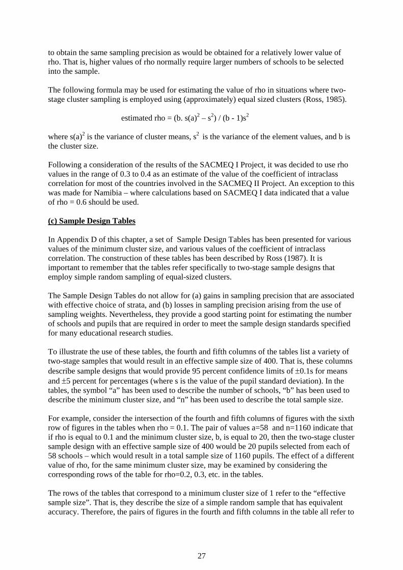
to obtain the same sampling precision as would be obtained for a relatively lower value of rho. That is, higher values of rho normally require larger numbers of schools to be selected into the sample. The following formula may be used for estimating the value of rho in situations where two-stage cluster sampling is employed using (approximately) equal sized clusters (Ross, 1985).

estimated rho = (b. s(a)2 – s2) / (b - 1)s2

where s(a)2 is the variance of cluster means, s2 is the variance of the element values, and b is the cluster size. Following a consideration of the results of the SACMEQ I Project, it was decided to use rho values in the range of 0.3 to 0.4 as an estimate of the value of the coefficient of intraclass correlation for most of the countries involved in the SACMEQ II Project. An exception to this was made for Namibia – where calculations based on SACMEQ I data indicated that a value of rho = 0.6 should be used. (c) Sample Design Tables In Appendix D of this chapter, a set of Sample Design Tables has been presented for various values of the minimum cluster size, and various values of the coefficient of intraclass correlation. The construction of these tables has been described by Ross (1987). It is important to remember that the tables refer specifically to two-stage sample designs that employ simple random sampling of equal-sized clusters. The Sample Design Tables do not allow for (a) gains in sampling precision that are associated with effective choice of strata, and (b) losses in sampling precision arising from the use of sampling weights. Nevertheless, they provide a good starting point for estimating the number of schools and pupils that are required in order to meet the sample design standards specified for many educational research studies. To illustrate the use of these tables, the fourth and fifth columns of the tables list a variety of two-stage samples that would result in an effective sample size of 400. That is, these columns describe sample designs that would provide 95 percent confidence limits of ±0.1s for means and ±5 percent for percentages (where s is the value of the pupil standard deviation). In the tables, the symbol “a” has been used to describe the number of schools, “b” has been used to describe the minimum cluster size, and “n” has been used to describe the total sample size. For example, consider the intersection of the fourth and fifth columns of figures with the sixth row of figures in the tables when rho = 0.1. The pair of values a=58 and n=1160 indicate that if rho is equal to 0.1 and the minimum cluster size, b, is equal to 20, then the two-stage cluster sample design with an effective sample size of 400 would be 20 pupils selected from each of 58 schools – which would result in a total sample size of 1160 pupils. The effect of a different value of rho, for the same minimum cluster size, may be examined by considering the corresponding rows of the table for rho=0.2, 0.3, etc. in the tables. The rows of the tables that correspond to a minimum cluster size of 1 refer to the “effective sample size”. That is, they describe the size of a simple random sample that has equivalent accuracy. Therefore, the pairs of figures in the fourth and fifth columns in the table all refer to

28

sample designs that have equivalent accuracy to a simple random sample of size 400. The second and third columns refer to an equivalent sample size of 1,600, and the final two pairs of columns refer to equivalent sample sizes of 178 and 100, respectively. (d) The Numbers of Schools and Pupils Required for this Study Using values of rho=0.3 (Botswana, Malawi, Mauritius, Swaziland, Uganda) and rho=0.4 (Kenya, Lesotho, Mozambique, South Africa, Tanzania, Zambia) in association with a minimum cluster size of 20 pupils indicated that there was a need to select (at least) 134 and 172 schools for these two groups of countries, respectively, in order to meet the SACMEQ II Project sampling requirements. In fact, additional schools were selected in most countries with the aim of achieving reasonably stable sample estimates within Regions. Exceptions to this approach were made for Namibia, the Seychelles, and Zanzibar. In Namibia, some calculations made using SACMEQ I data indicated that a value of rho = 0.6 should be used to plan the sample. As a result, at least 248 schools were required in Namibia. In the Seychelles and Zanzibar it was decided to include all schools in the defined target population.

Construction of Sampling Frames The defined target population definition was used to guide the construction of sampling frames from which the samples of schools were selected. The sampling frames were based on national lists of schools that included information about: school identification numbers, enrolment for the target population of Grade 6 pupils, and school regional location. The information used to construct the sampling frames was based on data that had been collected by the SACMEQ Ministries of Education for the most recent School Census. The sampling frame for each country provided a “listing” of the pupils in the defined target population without actually creating a physical list consisting of an entry for each and every pupil. For this study, the sampling frame needed to provide a complete coverage of the defined target population without being contaminated with incorrect entries, duplicate entries, or entries that referred to elements that were not part of the defined target population. Work commenced on the construction of SACMEQ II sampling frames in January 2000. For countries with high quality Educational Management Information Systems (EMIS) this task was very easy and was completed within a week. Other countries took up to six months to complete their sampling frames because of (a) major errors in EMIS data files, (b) difficulties in communicating information requirements to the Ministry staff responsible for EMIS functions, (c) difficulties in combining regional databases to form a single national sampling frame, (d) problems with inconsistent school numbering systems, and (e) changes in the geographical boundaries of regions during the time period between the implementations of the SACMEQ I and SACMEQ II Projects.

29

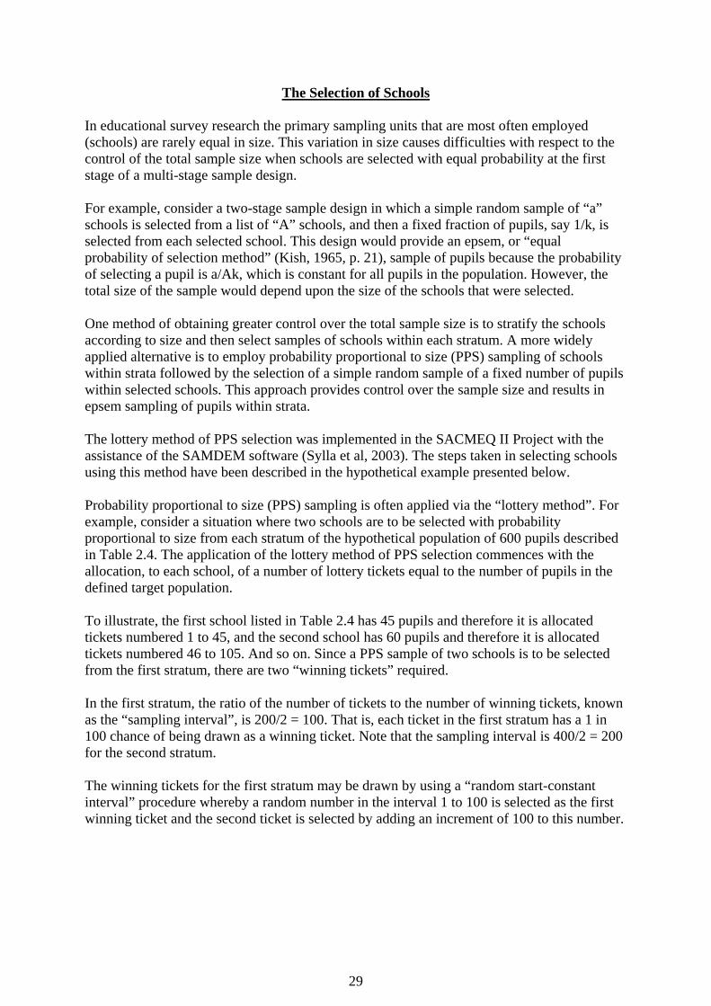
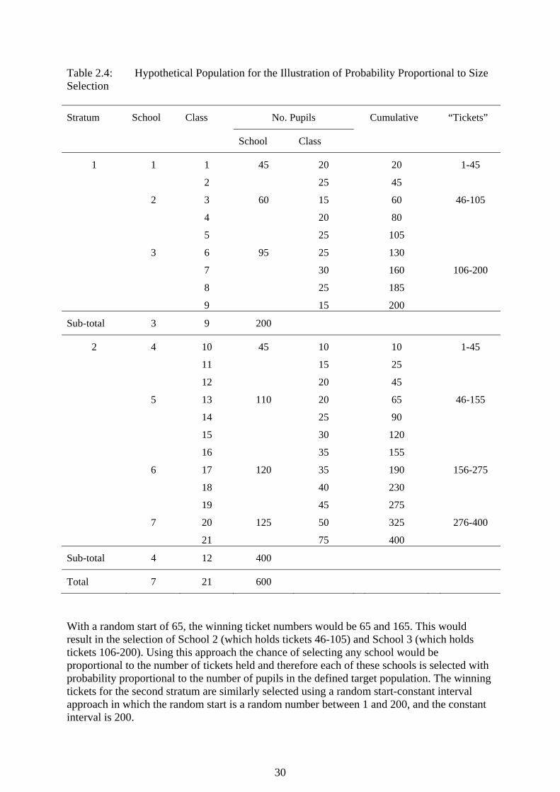
The Selection of Schools In educational survey research the primary sampling units that are most often employed (schools) are rarely equal in size. This variation in size causes difficulties with respect to the control of the total sample size when schools are selected with equal probability at the first stage of a multi-stage sample design. For example, consider a two-stage sample design in which a simple random sample of “a” schools is selected from a list of “A” schools, and then a fixed fraction of pupils, say 1/k, is selected from each selected school. This design would provide an epsem, or “equal probability of selection method” (Kish, 1965, p. 21), sample of pupils because the probability of selecting a pupil is a/Ak, which is constant for all pupils in the population. However, the total size of the sample would depend upon the size of the schools that were selected. One method of obtaining greater control over the total sample size is to stratify the schools according to size and then select samples of schools within each stratum. A more widely applied alternative is to employ probability proportional to size (PPS) sampling of schools within strata followed by the selection of a simple random sample of a fixed number of pupils within selected schools. This approach provides control over the sample size and results in epsem sampling of pupils within strata. The lottery method of PPS selection was implemented in the SACMEQ II Project with the assistance of the SAMDEM software (Sylla et al, 2003). The steps taken in selecting schools using this method have been described in the hypothetical example presented below. Probability proportional to size (PPS) sampling is often applied via the “lottery method”. For example, consider a situation where two schools are to be selected with probability proportional to size from each stratum of the hypothetical population of 600 pupils described in Table 2.4. The application of the lottery method of PPS selection commences with the allocation, to each school, of a number of lottery tickets equal to the number of pupils in the defined target population.

To illustrate, the first school listed in Table 2.4 has 45 pupils and therefore it is allocated tickets numbered 1 to 45, and the second school has 60 pupils and therefore it is allocated tickets numbered 46 to 105. And so on. Since a PPS sample of two schools is to be selected from the first stratum, there are two “winning tickets” required. In the first stratum, the ratio of the number of tickets to the number of winning tickets, known as the “sampling interval”, is 200/2 = 100. That is, each ticket in the first stratum has a 1 in 100 chance of being drawn as a winning ticket. Note that the sampling interval is 400/2 = 200 for the second stratum. The winning tickets for the first stratum may be drawn by using a “random start-constant interval” procedure whereby a random number in the interval 1 to 100 is selected as the first winning ticket and the second ticket is selected by adding an increment of 100 to this number.

30

Table 2.4: Hypothetical Population for the Illustration of Probability Proportional to Size Selection Stratum School Class No. Pupils Cumulative “Tickets”

School Class

1 1 1 45 20 20 1-45

2 25 45

2 3 60 15 60 46-105

4 20 80

5 25 105

3 6 95 25 130

7 30 160 106-200

8 25 185

9 15 200

Sub-total 3 9 200

2 4 10 45 10 10 1-45

11 15 25

12 20 45

5 13 110 20 65 46-155

14 25 90

15 30 120

16 35 155

6 17 120 35 190 156-275

18 40 230

19 45 275

7 20 125 50 325 276-400

21 75 400

Sub-total 4 12 400

Total 7 21 600

With a random start of 65, the winning ticket numbers would be 65 and 165. This would result in the selection of School 2 (which holds tickets 46-105) and School 3 (which holds tickets 106-200). Using this approach the chance of selecting any school would be proportional to the number of tickets held and therefore each of these schools is selected with probability proportional to the number of pupils in the defined target population. The winning tickets for the second stratum are similarly selected using a random start-constant interval approach in which the random start is a random number between 1 and 200, and the constant interval is 200.

31

The Selection of Pupils within Schools

A critical component of the sample design for the SACMEQ II Project was concerned with the selection of pupils within selected schools. It was decided that these selections should be placed under the control of trained data collectors – after they were provided with materials that would ensure that a simple random sample of pupils was selected in each selected school. The data collectors were informed that it was not acceptable to permit school principals or classroom teachers to have any influence over the sampling procedures within schools. These groups of people may have had a vested interest in selecting particular kinds of pupils, and this may have resulted in major distortions of sample estimates (Brickell, 1974). In the two SACMEQ Projects the data collectors initially explained to School Heads in selected schools that a “mechanical procedure” would be used to select the sample of 20 pupils. The data collectors then applied the following set of instructions in order to ensure that a simple random sample of pupils was selected. Step 1: Obtain Grade 6 register(s) of attendance. These registers were obtained for all Grade 6 pupils that attended normal (not “special”) classes. In multiple session schools, both morning and afternoon registers were obtained. Step 2: Assign sequential numbers to all Grade 6 pupils. A sequential number was then placed beside the name of each Grade 6 pupil. For example: Consider a school with one session and a total of 48 pupils in Grade 6. Commence by placing the number “1” beside the first pupil on the Register; than place the number “2” beside the second pupil on the Register; …etc. …; finally, place the number “48” beside the last pupil on the Register. Another example: Consider a school with 42 pupils in the morning session and 48 pupils in the afternoon session of Grade 5. Commence by placing the number “1” beside the first pupil on the morning register; … etc. …; then place a “42” beside the last pupil on the morning register; then place a “43” beside the first pupil on the afternoon register; … etc. …; finally place a “90” beside the last pupil on the afternoon register. Step 3: Locate the appropriate set of selection numbers. In Appendix E sets of “selection numbers” have been listed for a variety of school sizes. (Note that only the sets relevant for school sizes in the range 21 to 245 have been presented.) For example, if a school had 48 pupils in Grade 6, then the appropriate set of selection numbers was listed under the “R48” heading. Similarly, if a school had 90 Grade 5 pupils then the appropriate set of selection numbers was listed under the “R90” heading. Step 4: Use the appropriate set of selection numbers. After locating the appropriate set of selection numbers, these were used to select the sample of 20 pupils. The first selection number was used to locate the Grade 6 pupil with the same sequential number on the Register(s). The second selection number was used to locate the Grade 6 pupil with the same sequential number on the Register(s). This process was repeated in order to select 20 pupils

32

For example: From Appendix E we see that in a school with a total of 50 pupils in Grade 5 the first pupil selected has sequential number “2”; the second pupil selected has sequential number “4”; … etc. …; the twentieth pupil selected has sequential number “50”.

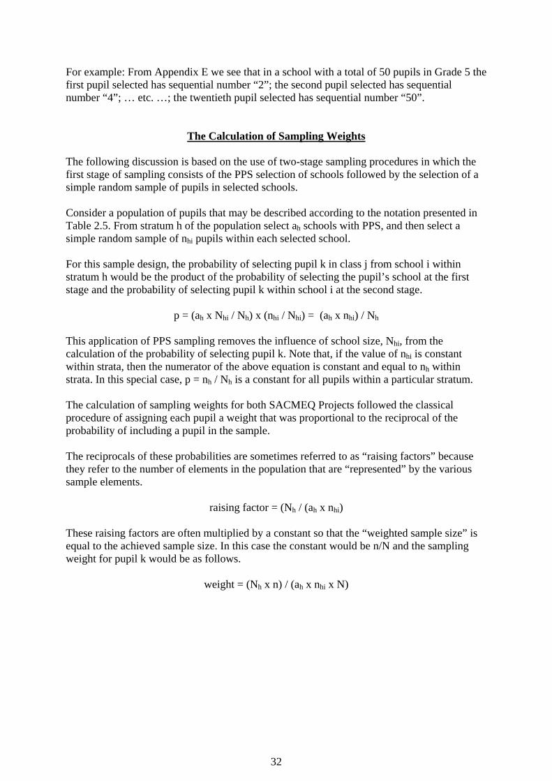
The Calculation of Sampling Weights The following discussion is based on the use of two-stage sampling procedures in which the first stage of sampling consists of the PPS selection of schools followed by the selection of a simple random sample of pupils in selected schools. Consider a population of pupils that may be described according to the notation presented in Table 2.5. From stratum h of the population select ah schools with PPS, and then select a simple random sample of nhi pupils within each selected school. For this sample design, the probability of selecting pupil k in class j from school i within stratum h would be the product of the probability of selecting the pupil’s school at the first stage and the probability of selecting pupil k within school i at the second stage.

p = (ah x Nhi / Nh) x (nhi / Nhi) = (ah x nhi) / Nh This application of PPS sampling removes the influence of school size, Nhi, from the calculation of the probability of selecting pupil k. Note that, if the value of nhi is constant within strata, then the numerator of the above equation is constant and equal to nh within strata. In this special case, p = nh / Nh is a constant for all pupils within a particular stratum. The calculation of sampling weights for both SACMEQ Projects followed the classical procedure of assigning each pupil a weight that was proportional to the reciprocal of the probability of including a pupil in the sample. The reciprocals of these probabilities are sometimes referred to as “raising factors” because they refer to the number of elements in the population that are “represented” by the various sample elements.

raising factor = (Nh / (ah x nhi) These raising factors are often multiplied by a constant so that the “weighted sample size” is equal to the achieved sample size. In this case the constant would be n/N and the sampling weight for pupil k would be as follows.

weight = (Nh x n) / (ah x nhi x N)

33

Table 2.5: Notation used in Discussion of Sample Designs

Units

Coverage of units Schools Classes Pupils

Total Sample Total Sample Total Sample

Population A A B B N n

Stratum h Ah ah Bh bh Nh nh

School i (Stratum h)

- - Bhi bhi Nhi nhi

Class j (School i in Stratum h)

- - - - Nhij nhij

Note: 1. The notation conventions for sample designs described in this manual have been listed in the above table. The table entries describe the number of “units” (schools, classes, or pupils) associated with each of four levels of “coverage” (population, stratum h, school i, or class j).

Note: 2. For example, the symbol A has been used to refer to the total number of schools

(“units”) in the population (“coverage”), whereas the symbol Ah has been used to describe the total number of schools (“units”) in stratum h (“coverage”). Similarly, the symbol n has been used to refer to the number of pupils in the sample, whereas the symbol nhij has been used to refer to the number of pupils in the sample associated with class j (situated in school i within stratum h).

In most “real” school system sampling situations, the number of pupils in the defined target population within each school listed on the sampling frame is different from the actual number of pupils. This occurs because sampling frames are usually developed from data collected at some earlier time – often a year prior to the selection of the sample of schools. That is, rather than finding Nhi pupils in school i within stratum h, we often find that there are Nhi (actual) pupils. In addition, due to occasional absenteeism on the day of data collection, instead of being able to test nhi pupils in a sample school we often only manage to collect data from nhi (actual) pupils. Given these two deviations, the actual probability (assuming random loss of data) of selecting a pupil in school i within stratum h may be written as follows.

34

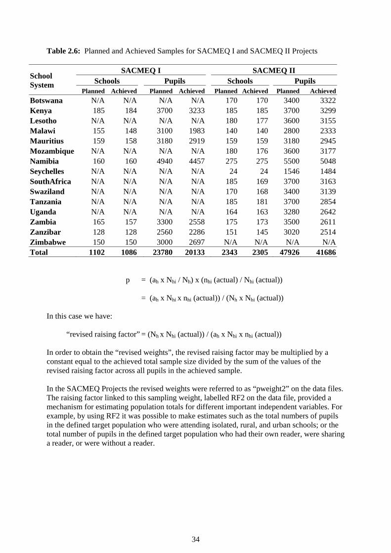
Table 2.6: Planned and Achieved Samples for SACMEQ I and SACMEQ II Projects

School System

SACMEQ I SACMEQ II Schools Pupils Schools Pupils

Planned Achieved Planned Achieved Planned Achieved Planned AchievedBotswana N/A N/A N/A N/A 170 170 3400 3322Kenya 185 184 3700 3233 185 185 3700 3299Lesotho N/A N/A N/A N/A 180 177 3600 3155Malawi 155 148 3100 1983 140 140 2800 2333Mauritius 159 158 3180 2919 159 159 3180 2945Mozambique N/A N/A N/A N/A 180 176 3600 3177Namibia 160 160 4940 4457 275 275 5500 5048Seychelles N/A N/A N/A N/A 24 24 1546 1484SouthAfrica N/A N/A N/A N/A 185 169 3700 3163Swaziland N/A N/A N/A N/A 170 168 3400 3139Tanzania N/A N/A N/A N/A 185 181 3700 2854Uganda N/A N/A N/A N/A 164 163 3280 2642Zambia 165 157 3300 2558 175 173 3500 2611Zanzibar 128 128 2560 2286 151 145 3020 2514Zimbabwe 150 150 3000 2697 N/A N/A N/A N/ATotal 1102 1086 23780 20133 2343 2305 47926 41686

p = (ah x Nhi / Nh) x (nhi (actual) / Nhi (actual))

= (ah x Nhi x nhi (actual)) / (Nh x Nhi (actual)) In this case we have: “revised raising factor” = (Nh x Nhi (actual)) / (ah x Nhi x nhi (actual)) In order to obtain the “revised weights”, the revised raising factor may be multiplied by a constant equal to the achieved total sample size divided by the sum of the values of the revised raising factor across all pupils in the achieved sample. In the SACMEQ Projects the revised weights were referred to as “pweight2” on the data files. The raising factor linked to this sampling weight, labelled RF2 on the data file, provided a mechanism for estimating population totals for different important independent variables. For example, by using RF2 it was possible to make estimates such as the total numbers of pupils in the defined target population who were attending isolated, rural, and urban schools; or the total number of pupils in the defined target population who had their own reader, were sharing a reader, or were without a reader.

35

Some Background Comments on the Calculation of Sampling Errors The sample designs employed in the SACMEQ Projects departed markedly from the usual “textbook model” of simple random sampling. This departure demanded that special steps be taken in order to calculate “sampling errors” (that is, measures of the stability of sample estimates of population characteristics). In the following discussion, a brief overview has been presented of various aspects of the general concept of “sampling error”. This has included a discussion of notions of “design effect”, “the effective sample size”, and the “Jackknife procedure” for estimating sampling errors. (a) Bias, Sampling Error, and Mean Square Error Consider a probability sample of n elements that is used to calculate the sample mean, x , as an estimate of the population mean, X . If an infinite set of samples of size n were drawn independently from this population and the sample mean calculated for each of these samples, then the average of the resulting sampling distribution of sample means, the expected value of x , could be denoted by E ( )x . The accuracy of the sample statistic, x , as an estimator of the population parameter, X , may be summarized in terms of the mean square error (MSE). The MSE is defined as the average of the squares of the deviations of all possible sample estimates from the value being estimated (Hansen, et al, 1953). MSE ( )x = ( )2XxE −

= ( )( )2xExE − + ( )( )2XxE − = variance of x + (bias of x )2 A sample design is unbiased if E ( )x = X . It is important to remember that “bias” is not a property of a single sample, but of the entire sampling distribution, and that it belongs neither to the selection nor the estimation procedure alone, but to both jointly. For most well designed samples in survey research, the bias is usually very small – tending towards zero with increasing sample size. The accuracy of sample estimates is therefore generally assessed in terms of the variance of x , denoted var ( )x , which quantifies the sampling stability of the values of x around their expected value E ( )x (b) The Accuracy of Individual Sample Estimates In educational settings the researcher is usually dealing with a single sample of data and not with all possible samples from a population. The variance of sample estimates therefore cannot be calculated in the manner described above. However, for many sample designs based on strict probability sampling methods, statistical theory may be used to provide estimates of the variance based on the internal evidence of a single sample of data. In the case of a simple random sample of n elements drawn without replacement from a population of N elements, the variance of the sample mean may be estimated from a single sample of data by using the following formula:

var(x) = (N - n) / N . s2/n

36

where s2 is the usual sample estimate of the variance of the element values in the population, (Kish, 1965 p. 41). For sufficiently large values of N, the value of the “finite population correction”, (N - n)/N, tends toward unity. The variance of the sample mean in this situation may therefore be estimated by s2/n. The sampling distribution of the sample mean is approximately normally distributed for many survey research situations. The approximation improves with increased sample size – even though the distribution of elements in the parent population may be far from normal. This characteristic of sampling distributions is known as the Central Limit Theorem and it occurs not only for the sample mean but also for most estimators commonly used to describe survey research results (Kish, 1965). From a knowledge of the properties of the normal distribution we know that we can be “68 percent confident” that the range x ± ( )xse includes the population mean, where x is the sample mean obtained from a single sample and ( )xse , often called the standard error, is the square root of ( )xvar . Similarly the range x ± 1.96 ( )xse will include the population mean with 95 percent confidence. While the above discussion has concentrated on sample means derived from simple random samples, the same approach may be used to establish confidence limits for many other statistics derived from various types of sample designs. For example, confidence limits may be calculated for complex statistics such as correlation coefficients, regression coefficients, and multiple correlation coefficients (Ross, 1978). (c) Comparison of the Accuracy of Probability Samples The accuracy of probability samples is usually considered by examining the variance associated with a particular sample estimate for a given sample size. This approach to the evaluation of sampling accuracy has generally been based on the recommendation put forward by Kish (1965) that the simple random sample design should be used as a standard for quantifying the accuracy of sample designs that incorporate such complexities as stratification and clustering. Kish introduced the term “deff” (design effect) to describe the ratio of the variance of the sample mean for a complex sample design (denoted c) to the variance of the sample mean for a simple random sample (denoted srs) of the same size.

That is, deff = ( ) ( )srsc xvar/xvar For the kinds of complex sample designs that are commonly used in educational research, the values of deff for many statistics are often greater than unity. Consequently, the accuracy of sample estimates may be grossly overestimated if formulae based on simple random sampling assumptions are used to calculate sampling errors. The potential for arriving at false conclusions by using incorrect sampling error calculations has been illustrated in a study carried out by Ross (1976). An alternative approach to comparing the accuracy of probability samples is to calculate the “effective sample size”. For a given complex sample design (with a sample size of nc), the effective sample size for a particular statistic (denoted n* below) is equal the size of a simple random sample that has the same variance. By using a little algebra (Ross and Rust, 1997) the

37

above equation may be transformed into an expression that relates the size of the complex sample, the design effect, and the effective sample size.

n* = nc/deff (d) Error estimation for complex probability samples The computational formulae required to estimate the variance of descriptive statistics, such as sample means, are available for some probability sample designs which incorporate complexities such as stratification and cluster sampling. However, for many commonly-employed statistics, the required formulae are not readily available for sample designs which depart markedly from the model of simple random sampling. These formulae are either enormously complicated or, ultimately, they prove resistant to mathematical analysis (Frankel, 1971). In the absence of suitable formulae, a variety of empirical techniques have emerged in recent years which provide “approximate variances that appear satisfactory for practical purposes” (Kish, 1978 p. 20). The most frequently applied empirical techniques may be divided into two broad categories: Subsample Replication and Taylor’s Series Approximation. In Subsample Replication a total sample of data is used to construct two or more subsamples and then a distribution of parameter estimates is generated by using each subsample. The subsample results are analysed to obtain an estimate of the parameter, as well as a confidence assessment for that estimate (Finifter, 1972 p. 114). The main approaches in using this technique have been Independent Replication (Deming, 1960), Jackknifing (Tukey, 1958), Balanced Repeated Replication (McCarthy, 1966). In the SACMEQ II Project it was decided calculate sampling errors by using the IIEPJACK software. This software was based on the Jackknife procedure, and its capacity to interface with the SPSS software system made it possible to quickly and easily prepare tabulations and associated sampling errors for all summary statistics employed in the research.

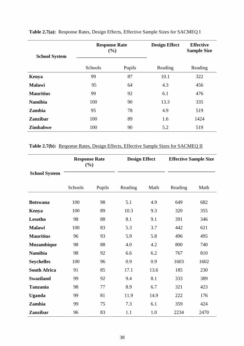
Evaluation of the SACMEQ Sample Designs (a) Response Rates In Table 2.6 the size of the planned and achieved samples have been presented for both the SACMEQ I and SACMEQ II Projects. The value of the achieved sample size as a percentage of the planned sample size represents the “response rate”. The response rate percentages for pupils and schools have been presented for the SACMEQ I Project in Table 2.7(a) and for the SACMEQ II Project in Table 2.7(b). The technical requirement for the SACMEQ research programme was that all countries should seek to achieve overall response rates of 90 percent for schools and 80 percent for pupils. From the first two columns of Table 2.7(a) it may be seen that for the SACMEQ I Project all countries achieved the required response rate for schools - however Malawi and Zambia experienced major losses of pupil data within responding schools and as a result achieved pupil response rates of only 64 percent and 78 percent, respectively. The SACMEQ II response rates presented in Table 2.7(b) showed that all countries satisfied the required response rate for schools – however both Tanzania and Zambia experienced considerable loss of data within schools. The pupil response rates for these countries were 77 percent and 75 percent, respectively, - which were fairly close to the goal of an 80 percent response rate.

38

Table 2.7(a): Response Rates, Design Effects, Effective Sample Sizes for SACMEQ I

School System

Response Rate (%)

Design Effect

Effective Sample Size

Schools Pupils Reading Reading

Kenya 99 87 10.1 322

Malawi 95 64 4.3 456

Mauritius 99 92 6.1 476

Namibia 100 90 13.3 335

Zambia 95 78 4.9 519

Zanzibar 100 89 1.6 1424

Zimbabwe 100 90 5.2 519 Table 2.7(b): Response Rates, Design Effects, Effective Sample Sizes for SACMEQ II

School System

Response Rate (%)

Design Effect

Effective Sample Size

Schools

Pupils

Reading

Math

Reading

Math

Botswana 100 98

5.1

4.9

649

682

Kenya 100 89 10.3 9.3 320 355

Lesotho 98 88 8.1 9.1 391 346

Malawi 100 83 5.3 3.7 442 621

Mauritius 96 93 5.9 5.8 496 495

Mozambique 98 88 4.0 4.2 800 740

Namibia 98 92 6.6 6.2 767 810

Seychelles 100 96 0.9 0.9 1603 1602

South Africa 91 85 17.1 13.6 185 230

Swaziland 99 92 9.4 8.1 333 389

Tanzania 98 77 8.9 6.7 321 423

Uganda 99 81 11.9 14.9 222 176

Zambia 99 75 7.3 6.1 359 424

Zanzibar 96 83 1.1 1.0 2234 2470

39

Table 2.8 : Values of the Coefficient of Intraclass Correlation for the Tests used in the SACMEQ I and SACMEQ II Projects

School System

SACMEQ I SACMEQ II

Reading Reading Mathematics roh roh roh

Botswana N/A 26 22

Kenya 42 45 38

Lesotho N/A 39 30

Malawi 24 29 15

Mauritius 25 26 25

Mozambique N/A 30 21

Namibia 65 60 53

Seychelles N/A 8 8

South Africa N/A 70 64

Swaziland N/A 37 26

Tanzania N/A 34 26

Uganda N/A 57 65

Zambia 27 32 22

Zanzibar 17 25 33

Zimbabwe 27 N/A N/A

SACMEQ II 33 37 32 (b) Intraclass Correlations The coefficient of intraclass correlation may be used to measure the proportion of variance in pupil test scores that may be attributed to variation among schools. The coefficient is functionally related to the design effect such that a high value of the coefficient results in a high value of the design effect. This linkage between the coefficient of intraclass correlation and the design effect implies that more sample schools are required in a country where the coefficient takes a high value than are required in a country where the coefficient takes a low value (in order to reach the same level of sampling accuracy). In Table 2.8 the values of the coefficient of intraclass correlation have been presented for the pupil tests used in the SACMEQ I and SACMEQ II Projects. For both the reading and mathematics tests used in the SACMEQ II Project, the lowest values of the coefficient occurred for the Seychelles (0.08), Botswana and Mauritius (both around 0.25). In contrast, values in the range 0.50 to 0.70 occurred for Namibia, South Africa., and

40

Uganda. The high values for Namibia were known prior to the completion of the SACMEQ II sample designs because they were calculated to be around 0.65 for the SACMEQ I reading test, and therefore a much larger sample of Namibian schools (275) was selected. Unfortunately, the high values for South Africa and Uganda were not known beforehand, and the sample designs for these countries were based on “guesstimates” that the value of the intraclass correlation for each country was around 0.4. As a result the number of schools in the sample designs for these two countries was too small – which resulted in a shortfall in the effective sample sizes for these countries. (c) Design Effects and Effective Sample Sizes The design effect (Kish, 1965) provides an indicator of the increase in sampling variance that occurs for a complex sample in comparison with a simple random sample of the same size. The effective sample size (Ross, 1987) for a complex sample represents the size of a simple random that would have the same sampling accuracy as the complex sample. In the final columns of Table 2.7(b) and Table 2.7(b) the “design effect” and the “effective sample size” have been presented for the SACMEQ I reading test and the SACMEQ II reading and mathematics tests. In the SACMEQ I Project two countries (Kenya and Namibia) had effective sample sizes that fell below the target value of 400 pupils; whereas in the SACMEQ II Project five countries (Kenya, Namibia, South Africa, Swaziland, and Seychelles) fell below the target value. In the SACMEQ II Project, two school systems, South Africa and Uganda, fell far below the required target of an effective sample size of 400 pupils. In South Africa the values were 185 and 230 for reading and mathematics, respectively, and in Uganda the values were 222 and 176 for reading and mathematics, respectively. The values of the “design effect” and the “effective sample size” have also been presented for various variables and a single country (Botswana) in Tables 2.9(a) and 2.9(b). To illustrate, consider the design effect and effective sample size values in Table 2.9(a) for the pupil average reading score for Botswana overall. The design effect for this variable was 5.12, which indicated that the variance of the sample estimate of the variance of pupil reading scores for Botswana was 5.12 times larger than would be expected for a simple random sample of the same size (3322 pupils). The effective sample size for this variable indicated that the complex sample of 3322 pupils had a sampling variance that was the same as would have been obtained by employing a simple random sample of 649 pupils. In Table 2.9(a) and Table 2.9(b) values of the design effect and the effective sample size have been presented for a selection of variables at different “levels” (pupil, teacher, and school head). The word “levels” here refers to the structure of the basic data file for the SACMEQ I and SACMEQ II Projects – in which the units of analysis were pupils – with teacher and school head data being disaggregated over pupils. This disaggregation of teacher and school head data in order to construct a “between-pupils” data file resulted in effective sample sizes for teacher variables that approached the total number of teachers, and effective sample sizes for school head variables that approached the total number of schools. To illustrate, for Botswana overall the effective sample size for the “teacher academic education” variable was 311 (close to the total number of teachers in the survey), and for the “pupil-toilet ratio” variable was 171 (close to the total number of schools in the survey).

41

Table 2.9(a). Botswana overall: Sampling errors (SE), design effects, and actual/effective sample sizes for selected variables at the pupil, teacher, and school head levels

Variable Mean % SE Design Effect Sample Size

Actual Effective

At pupil level

Pupil speaking English at home Pupil being given reading homework Reading pupil scores Mathematics pupil scores

521.1 512.9

74.0 40.1

1.34 1.47 3.47 3.15

3.08 2.99 5.12 4.87

3322 3322 3322 3321

1077 1111 649 682

Average 3.38 3322 2141 At reading teacher level 12.39 3312 (393) 273

Teacher academic education Total classroom resources Available classroom library Sex of teacher

2.56 6.43

81.2 66.7

0.05 0.12 2.50 2.68

10.69 14.59 13.65 10.61

3322 (393)3322 (393)3322 (393)3282 (391)

311 228 243 309

Average 12.39 3312 (393) 273

At school head level

Pupil-toilet ratio Total school resources Available school staff room Sex of school head

44.43 9.81

74.8 53.4

2.15 0.24 3.43 3.89

19.43 18.93 20.79 20.25

3322 (170)3322 (170)3322 (170)3322 (170)

171 176 160 164

Average 19.85 3322 (170) 168

SACMEQII 2000-02 Sampling.doc 01/10/2008 42

Table 2.9 (b) Botswana Central Region: Sampling errors (SE), design effects, and actual/effective sample sizes for selected variables at the pupil, teacher, and school head levels

Variable Mean % SE Design Effect Sample Size

Actual Effective

At pupil level

Pupil speaking English at home Pupil being given reading homework Reading pupil scores Mathematics pupil scores

506.1 506.2

66.7 40.4

3.55 3.71 6.56 5.57

2.80 2.81 3.51 2.65

493 493 493 493

176 175 140 186

Average 2.46 493 268 At reading teacher level

Teacher academic education Total classroom resources Available classroom library Sex of teacher

2.6 6.1

81.7 71.5

0.13 0.33 6.59 7.45

7.41 14.06 14.28 13.45

493 (64) 493 (64) 493 (64) 493 (64)

67 35 35 37

Average 12.30 493 (64) 44

At school head level

Pupil-toilet ratio Total school resources Available school staff room Sex of school head

40.6 10.4

72.1 52.1

4.56 0.66 9.89 10.49

20.62 19.31 23.98 21.75

493 (25) 493 (25) 493 (25) 493 (25)

24 26 21 23

Average 21.42 493 (25) 24

SACMEQII 2000-02 Sampling.doc 01/10/2008 43

(d) Sampling Errors The calculation of sampling errors for the SACMEQ Projects needed to acknowledge that the samples were not simple random samples - but rather complex two-stage cluster samples that included weighting adjustments to compensate for variations in selection probabilities. The IIEP’s specialized sampling software (IIEPJACK) was used to make these calculations. In the SACMEQ I and SACMEQ II national policy reports the sampling errors were calculated for each summary statistic, and they were labelled “SE” in the completed Dummy Tables. For example, consider the statistics reported for Botswana overall in Table 2.9(a) and the Central Region of Botswana in Table 2.9(b). In Table 2.9(a) the pupil average reading score for Botswana overall was 521.1 and the standard error of sampling was 3.47. These figures indicated that one could be 95 percent confident that the population average for pupils in Botswana on the reading test was within the following limits: 521.1 + 2(3.47). That is, between 514.2 and 528.0. Similarly, in Table 2.9(b) the pupil average reading score for the Central Region in Botswana was 506.1 and the standard error of sampling was 6.56. These figures indicated that one could be 95 percent confident that the population value for pupils in Botswana’s Central Region was within the following limits: 506.1 + 2(6.56). That is, between 493.0 and 519.2. When data are collected using multi-stage sample designs from sources at different levels of aggregation (pupil, teacher, school) a great deal of care needs to be taken in interpreting the stability of sample estimates of population characteristics. For the SACMEQ Projects, the data analyses were undertaken at the between-pupils level. That is, data collected from teachers and school heads were disaggregated across the pupil data files before the data analyses were undertaken. The interaction of sample design and level of data analysis required that extra caution be used in interpreting estimates obtained by using information from teachers or school heads. The sampling errors of estimates derived from these two “disaggregated sources” were far larger than figures generated by using standard statistical software packages.