OLIVEIRA Vygotsky Aprendizado e desenvolvimento um processo socio historico
Upload
khangminh22Category
view
1download
0
MACHINE LEARNING-BASED PROBABILISTIC STOPPING RULE FORTHE GRASP METAHEURISTIC
Guilherme Caeiro de Mattos
Dissertação de Mestrado apresentada aoPrograma de Pós-graduação em Engenhariade Sistemas e Computação, COPPE, daUniversidade Federal do Rio de Janeiro, comoparte dos requisitos necessários à obtenção dotítulo de Mestre em Engenharia de Sistemas eComputação.
Orientadores: Luidi Gelabert SimonettiPriscila Machado Vieira Lima
Rio de JaneiroDezembro de 2021

MACHINE LEARNING-BASED PROBABILISTIC STOPPING RULE FORTHE GRASP METAHEURISTIC
Guilherme Caeiro de Mattos
DISSERTAÇÃO SUBMETIDA AO CORPO DOCENTE DO INSTITUTOALBERTO LUIZ COIMBRA DE PÓS-GRADUAÇÃO E PESQUISA DEENGENHARIA DA UNIVERSIDADE FEDERAL DO RIO DE JANEIROCOMO PARTE DOS REQUISITOS NECESSÁRIOS PARA A OBTENÇÃO DOGRAU DE MESTRE EM CIÊNCIAS EM ENGENHARIA DE SISTEMAS ECOMPUTAÇÃO.
Orientadores: Luidi Gelabert SimonettiPriscila Machado Vieira Lima
Aprovada por: Prof. Luidi Gelabert SimonettiProf. Isabel Cristina Mello RossetiProf. Valmir Carneiro Barbosa
RIO DE JANEIRO, RJ – BRASILDEZEMBRO DE 2021

Mattos, Guilherme Caeiro deMachine Learning-Based Probabilistic Stopping Rule for
the GRASP Metaheuristic/Guilherme Caeiro de Mattos. –Rio de Janeiro: UFRJ/COPPE, 2021.
XIII, 107 p.: il.; 29, 7cm.Orientadores: Luidi Gelabert Simonetti
Priscila Machado Vieira LimaDissertação (mestrado) – UFRJ/COPPE/Programa de
Engenharia de Sistemas e Computação, 2021.Referências Bibliográficas: p. 45 – 47.1. Stopping Rule. 2. GRASP. 3. Machine Learning.
I. Simonetti, Luidi Gelabert et al. II. Universidade Federaldo Rio de Janeiro, COPPE, Programa de Engenharia deSistemas e Computação. III. Título.
iii

Agradecimentos
Primeiramente, gostaria de utilizar este espaço para agradecer aos meus orientadoresLuidi Gelabert Simonetti e Priscila Machado Vieira Lima, assim como ao ProfessorFelipe Maia Galvão França, que também apoiou este trabalho em todas as suasetapas.
Agredeço também aos autores do artigo "Probabilistic stopping rules for GRASPheuristics and extensions" por proverem os códigos que fomentaram seu trabalho,assim como ao Núcleo de Atendimento à Computação de Alto Desempenho da Uni-versidade Federal do Rio de Janeiro por permitir a utilização de recursos computa-cionais do supercomputador Lobo Carneiro.
Finalmente, agradeço ao Conselho Nacional de Desenvolvimento Científico eTecnológico (CNPq) por ajudar a financiar este trabalho através fornecimento debolsa de fomento, e à Coordenação de Aperfeiçoamento de Pessoal de Nível Supe-rior (CAPES) por apoio provido ao autor deste texto em outras fases de sua vidaacadêmica.
iv

Resumo da Dissertação apresentada à COPPE/UFRJ como parte dos requisitosnecessários para a obtenção do grau de Mestre em Ciências (M.Sc.)
PARADA PROBABILÍSTICA BASEADA EM APRENDIZADO DE MÁQUINAPARA A METAHEURÍSTICA GRASP
Guilherme Caeiro de Mattos
Dezembro/2021
Orientadores: Luidi Gelabert SimonettiPriscila Machado Vieira Lima
Programa: Engenharia de Sistemas e Computação
Metaheurísticas, como Simulated Annealing, Ant Colony, Algoritmos Genéti-cos e GRASP, são métodos genéricos que são normalmente aplicados a problemascomputacionalmente difíceis. Porém, elas normalmente carecem de um critério deparada efetivo, recorrendo a opções genéricas que resultam em desperdício de re-cursos computacionais e de tempo. A fim de mitigar esse problema, existe para ametaheurística GRASP um critério de parada probabilístico que utiliza a funçãode distribuição acumulada (FDA) para calcular, a partir de uma dada iteração, aprobabilidade de melhorar a solução em iterações futuras. No entanto, apesar deefetivo, ele possui suas próprias deficiências. Especificamente, o cálculo da FDAé relativamente lento e as probabilidades estimadas, em muitos casos, podem di-vergir significativamente da probabilidade observada em execuções suficientementelongas. Neste trabalho, propõe-se uma alternativa ao critério de parada probabilís-tica baseada em aprendizado de máquina. Esta dissertação mostra que, ao substituira FDA por modelos baseados em árvore, é possível reduzir o tempo necessário paraestimar probabilidades e diminuir a divergência com a probabilidade observada emexecuções do GRASP. Também é mostrado que é possível, para um modelo treinadosobre execuções de uma instância de um problema, generalizar para instâncias domesmo ou de outros problemas, mas com limitações.
v

Abstract of Dissertation presented to COPPE/UFRJ as a partial fulfillment of therequirements for the degree of Master of Science (M.Sc.)
MACHINE LEARNING-BASED PROBABILISTIC STOPPING RULE FORTHE GRASP METAHEURISTIC
Guilherme Caeiro de Mattos
December/2021
Advisors: Luidi Gelabert SimonettiPriscila Machado Vieira Lima
Department: Systems Engineering and Computer Science
Metaheuristics, like Simulated Annealing, Ant Colony, Genetic Algorithms andGRASP, are generic methods that are applied to solve problems that are compu-tationally hard. However, they usually lack an effective stopping criterion, relyingon generic options that usually result in a waste of computational resources andtime. Seeking to mitigate that problem, there is a probabilistic stopping criterionfor GRASP that uses the cumulative distribution function (CDF) to calculate, fora given iteration, the probability of improving the current solution in future itera-tions. Yet, that criterion also has its own drawbacks. Specifically, the CDF can berelatively slow to calculate and the probabilities it estimates, in many cases, can sig-nificantly diverge from the probabilities observed in sufficiently large executions. Inthis work, a machine learning-based alternative to the probabilistic stopping rule isproposed. This dissertation shows that, by replacing the CDF with a tree-based ma-chine learning model, it is possible to reduce the time taken to estimate a probabilityand reduce the divergence between that probability and the probability observed insufficiently large executions. It is also shown that it is possible for a model trainedon a given instance, of a given problem, to generalize to other instances, even fromother problems, but with limitations.
vi

Contents
List of Figures ix
List of Tables xii
1 Introduction 11.1 Motivation . . . . . . . . . . . . . . . . . . . . . . . . . . . . . . . . . 11.2 Contributions . . . . . . . . . . . . . . . . . . . . . . . . . . . . . . . 21.3 Text Outline . . . . . . . . . . . . . . . . . . . . . . . . . . . . . . . . 2
2 Background 42.1 A Decision Model for GRASP Metaheuristic . . . . . . . . . . . . . . 4
2.1.1 GRASP . . . . . . . . . . . . . . . . . . . . . . . . . . . . . . 42.1.2 Probabilistic Stopping Rule . . . . . . . . . . . . . . . . . . . 5
2.2 Machine Learning Based Decision Models . . . . . . . . . . . . . . . . 62.2.1 Decision Tree Regression . . . . . . . . . . . . . . . . . . . . . 62.2.2 Random Forest Regression . . . . . . . . . . . . . . . . . . . . 92.2.3 Extreme Gradient Boosting . . . . . . . . . . . . . . . . . . . 10
2.3 Test Optimization Problems . . . . . . . . . . . . . . . . . . . . . . . 122.3.1 Set k-Covering . . . . . . . . . . . . . . . . . . . . . . . . . . 122.3.2 Quadratic Assignment . . . . . . . . . . . . . . . . . . . . . . 13
3 AIISR: AI Inspired Stopping Rule For GRASP Metaheuristic 143.1 Overview . . . . . . . . . . . . . . . . . . . . . . . . . . . . . . . . . . 143.2 Datasets . . . . . . . . . . . . . . . . . . . . . . . . . . . . . . . . . . 15
3.2.1 Selected Instances . . . . . . . . . . . . . . . . . . . . . . . . . 183.2.2 Prominent Features . . . . . . . . . . . . . . . . . . . . . . . . 193.2.3 Normalization . . . . . . . . . . . . . . . . . . . . . . . . . . . 20
3.3 Feature Selection . . . . . . . . . . . . . . . . . . . . . . . . . . . . . 223.4 Parameter Selection . . . . . . . . . . . . . . . . . . . . . . . . . . . . 23
3.4.1 Decision Tree Regression . . . . . . . . . . . . . . . . . . . . . 243.4.2 Random Forest Regression . . . . . . . . . . . . . . . . . . . . 253.4.3 Extreme Gradient Boosting . . . . . . . . . . . . . . . . . . . 25
vii

4 Experimental Results 274.1 Computational Environment . . . . . . . . . . . . . . . . . . . . . . . 274.2 Evaluation on Unseen Instances . . . . . . . . . . . . . . . . . . . . . 284.3 Evaluation on Unseen Problems . . . . . . . . . . . . . . . . . . . . . 344.4 Model Choice . . . . . . . . . . . . . . . . . . . . . . . . . . . . . . . 40
5 Conclusions 425.1 Final Remarks . . . . . . . . . . . . . . . . . . . . . . . . . . . . . . . 425.2 Future Works . . . . . . . . . . . . . . . . . . . . . . . . . . . . . . . 43
References 45
A Instance’s Lower and Upper Bounds 48
B Error Heatmaps and Error Tables 50
C Stopping Rule in Action 63
viii

List of Figures
2.1 A decision tree for deciding on whether to play tennis or not. . . . . . 7
3.1 Average number of minimum changes at every 100 000 iterations inexecutions of the datasets employed for model training. On the x-axis,1 represents the interval (1, 100 000), 2 the interval (100 000, 200 000),3 the interval (200 000, 300 000), and so on. . . . . . . . . . . . . . . . 16
4.1 Fitting of the estimates of a decision tree regressor, trained on thescp42 dataset using the features (best_cost, best), when evaluatingthe first 1 000 iterations of a scp55 execution. . . . . . . . . . . . . . 29
4.2 Fitting of the estimates of a decision tree regressor, trained on thescp42 dataset using the features (best_cost, best), when evaluatingthe first 1 000 iterations of a scp55 execution. . . . . . . . . . . . . . 30
4.3 Fitting of the estimates of a decision tree regressor, trained on thescp42 dataset using the features (best_cost, best), when evaluatingthe first 1 000 iterations of a scpb5 execution. . . . . . . . . . . . . . 30
4.4 RMSEAV G for decision tree regressors, trained on SCP instances us-ing features (best_cost, best), when evaluated on datasets from otherSCP instances. . . . . . . . . . . . . . . . . . . . . . . . . . . . . . . 31
4.5 RMSEAV G for random forest regressors, trained on SCP instances us-ing features (best_cost, best), when evaluated on datasets from otherSCP instances. . . . . . . . . . . . . . . . . . . . . . . . . . . . . . . 31
4.6 RMSEAV G for XGBoost regressors, trained on SCP instances usingfeatures (best_cost, best), when evaluated on datasets from other SCPinstances. . . . . . . . . . . . . . . . . . . . . . . . . . . . . . . . . . 32
4.7 RMSEAV G for decision tree regressors, trained on QAP instances us-ing features (best_cost, best), when evaluated on datasets from otherQAP instances. . . . . . . . . . . . . . . . . . . . . . . . . . . . . . . 32
4.8 RMSEAV G for random forest regressors, trained on QAP instancesusing features (best_cost, best), when evaluated on datasets fromother QAP instances. . . . . . . . . . . . . . . . . . . . . . . . . . . . 33
ix

4.9 RMSEAV G for XGBoost regressors, trained on QAP instances us-ing features (best_cost, best), when evaluated on datasets from otherQAP instances. . . . . . . . . . . . . . . . . . . . . . . . . . . . . . . 33
4.10 RMSEAV G for decision tree regressors, trained on SCP instancesusing features (iteration, iterations_since_last_min, iterations_-since_best_cost, total_single_mins_found), when evaluated ondatasets from other SCP instances. . . . . . . . . . . . . . . . . . . . 34
4.11 RMSEAV G for decision tree regressors, trained on QAP instancesusing features (iteration, iterations_since_last_min, iterations_-since_best_cost, total_single_mins_found), when evaluated ondatasets from other QAP instances. . . . . . . . . . . . . . . . . . . . 34
4.12 RMSEAV G for decision tree regressors, trained using features (best_-cost, best), when evaluated on datasets from different instances andproblems. . . . . . . . . . . . . . . . . . . . . . . . . . . . . . . . . . 35
4.13 RMSEAV G for decision tree regressors, trained using features (itera-tion, cost, best), when evaluated on datasets from different instancesand problems. . . . . . . . . . . . . . . . . . . . . . . . . . . . . . . . 36
4.14 RMSEAV G for XGBoost regressors, trained using features (itera-tion, iterations_since_last_min, iterations_since_best_cost, total_-single_mins_found), when evaluated on datasets from different in-stances and problems. . . . . . . . . . . . . . . . . . . . . . . . . . . 36
B.1 RMSEAV G for decision tree regressors, trained using features (best_-cost, best), when evaluated on datasets from different instances andproblems. . . . . . . . . . . . . . . . . . . . . . . . . . . . . . . . . . 50
B.2 RMSEAV G for decision tree regressors, trained using features (it-eration, cost, best_cost), when evaluated on datasets from differentinstances and problems. . . . . . . . . . . . . . . . . . . . . . . . . . 51
B.3 RMSEAV G for decision tree regressors, trained using features (itera-tion, cost, best), when evaluated on datasets from different instancesand problems. . . . . . . . . . . . . . . . . . . . . . . . . . . . . . . . 51
B.4 RMSEAV G for decision tree regressors, trained using features (itera-tion, cost, best_cost, best), when evaluated on datasets from differentinstances and problems. . . . . . . . . . . . . . . . . . . . . . . . . . 52
B.5 RMSEAV G for decision tree regressors, trained using features (it-eration, iterations_since_last_min, iterations_since_best_cost, to-tal_single_mins_found), when evaluated on datasets from differentinstances and problems. . . . . . . . . . . . . . . . . . . . . . . . . . 52
x

B.6 RMSEAV G for random forest regressors, trained using features(best_cost, best), when evaluated on datasets from different instancesand problems. . . . . . . . . . . . . . . . . . . . . . . . . . . . . . . . 53
B.7 RMSEAV G for random forest regressors, trained using features (it-eration, cost, best_cost), when evaluated on datasets from differentinstances and problems. . . . . . . . . . . . . . . . . . . . . . . . . . 53
B.8 RMSEAV G for random forest regressors, trained using features (iter-ation, cost, best), when evaluated on datasets from different instancesand problems. . . . . . . . . . . . . . . . . . . . . . . . . . . . . . . . 54
B.9 RMSEAV G for random forest regressors, trained using features (itera-tion, cost, best_cost, best), when evaluated on datasets from differentinstances and problems. . . . . . . . . . . . . . . . . . . . . . . . . . 54
B.10 RMSEAV G for random forest regressors, trained using features (it-eration, iterations_since_last_min, iterations_since_best_cost, to-tal_single_mins_found), when evaluated on datasets from differentinstances and problems. . . . . . . . . . . . . . . . . . . . . . . . . . 55
B.11 RMSEAV G for XGBoost regressors, trained using features (best_-cost, best), when evaluated on datasets from different instances andproblems. . . . . . . . . . . . . . . . . . . . . . . . . . . . . . . . . . 55
B.12 RMSEAV G for XGBoost regressors, trained using features (iteration,cost, best_cost), when evaluated on datasets from different instancesand problems. . . . . . . . . . . . . . . . . . . . . . . . . . . . . . . . 56
B.13 RMSEAV G for XGBoost regressors, trained using features (iteration,cost, best), when evaluated on datasets from different instances andproblems. . . . . . . . . . . . . . . . . . . . . . . . . . . . . . . . . . 56
B.14 RMSEAV G for XGBoost regressors, trained using features (iteration,cost, best_cost, best), when evaluated on datasets from different in-stances and problems. . . . . . . . . . . . . . . . . . . . . . . . . . . 57
B.15 RMSEAV G for XGBoost regressors, trained using features (itera-tion, iterations_since_last_min, iterations_since_best_cost, total_-single_mins_found), when evaluated on datasets from different in-stances and problems. . . . . . . . . . . . . . . . . . . . . . . . . . . 57
xi

List of Tables
2.1 Input variables and their possible values. . . . . . . . . . . . . . . . . 7
3.1 Characteristics of the SCP instances. . . . . . . . . . . . . . . . . . . 183.2 Characteristics of the QAP instances. . . . . . . . . . . . . . . . . . . 183.3 Features derived from an iteration. . . . . . . . . . . . . . . . . . . . 193.4 Range of the features that are independent from cost. . . . . . . . . . 203.5 Average of the correlation between the features and remaining_mins
across a series of different executions, from different instances andproblems. . . . . . . . . . . . . . . . . . . . . . . . . . . . . . . . . . 22
3.6 Combinations of features evaluated in this work. . . . . . . . . . . . . 233.7 Cross-validation scores observed for decision tree regressors trained
on scp42 (left) and tai100a (right) datasets, using the combinationof features (best_cost, best) and varying maximum depths. Trainingtime refers to the time taken to train the final model of the cross-validation. . . . . . . . . . . . . . . . . . . . . . . . . . . . . . . . . . 24
3.8 Cross-validation scores observed for random forest regressors trainedon the scp42 dataset, using the combination of features (best_cost,best) and varying the number of trees and maximum depth. Trainingtime refers to the time taken to train the final model of the cross-validation. . . . . . . . . . . . . . . . . . . . . . . . . . . . . . . . . . 25
3.9 Cross-validation scores observed for XGBoost regressors trained onthe scp42 dataset, using the combination of features (best_cost, best)and varying the number of trees and maximum depth. Training timerefers to the time taken to train the final model of the cross-validation. 26
4.1 Error RMSEAV G for the XGboost model trained on scp42 instancesusing features (iteration, iterations_since_last_min, iterations_-since_best_cost, total_single_mins_found). . . . . . . . . . . . . . . 37
4.2 Error RMSEAV G for the Decision Tree Regressor model trained onscp42 instances using features (iteration, cost, best). . . . . . . . . . . 38
xii

4.3 Comparison between the CDF-based estimator and four machinelearning models when evaluating 170 different instances (45 SCP and125 QAP). In all cases, the CDF-based estimator was only executedin the first iteration of an execution and during minimum changes. . . 40
A.1 SCP instances and their respective lower and upper bounds. . . . . . 48A.2 QAP instances and their respective lower and upper bounds. . . . . . 49
B.1 RMSEAV G observed for the probabilistic stopping rule of RIBEIROet al. [1] and for different machine learning models when applied tomultiple SCP and QAP instances. (i) are results obtained when theestimators are executed only in the first iteration and on changes ofminimum cost, while in (ii) the estimators are also executed at every50 iterations. Feature set codes come from Table 3.6. . . . . . . . . . 58
C.1 Aggregate results for estimation time. Feature sets are from Table 3.6. 64C.2 Comparison between the ML-based and the CDF-based stopping rules
on 20 different instances (10 QAP and 10 SCP). Feature set codescome from Table 3.6. . . . . . . . . . . . . . . . . . . . . . . . . . . . 65
xiii

Chapter 1
Introduction
In this chapter, the problem that motivates this work is presented, as well as a briefdescription of the contributions effectively achieved and of the text structure.
1.1 Motivation
Metaheuristics, like Simulated Annealing, Genetic Algorithms, Ant Colony, TabuSearch and GRASP are generally employed to problems that are computationallyhard, that do not have known optimal solution, where they perform a set of genericprocedures in order to achieve sufficiently good solutions. However, despite theirsuccess in producing solutions to those problems, they usually lack an effectivestopping criterion and decide on whether they should stop searching for an improvedsolution based on criteria like a total number of iterations, the total execution time,a number of iterations without improvement to the best solution and other optionsthat commonly lead to an unnecessary waste in time and in computational resources.
That waste usually happens because of two different situations. The first isknown as early stopping and occurs when the execution stops a few iterations awayfrom an improved solution. Having no way to know that a better solution is nearby,the metaheuristic throws away all the computational resources that it spends fromthe moment it finds the current best solution up until the moment it stops theexecution, despite the fact that it could have improved the solution had it continuedthe execution for a few more iterations.
The second situation, on the other hand, happens when the optimal solution, ora very good local minimum, is found. In those cases, the metaheuristic continues tosearch for a better solution without knowing that there is very little or no chance forone to be found and, consequently, wastes time and computational resources onceagain.
In the context of the GRASP metaheuristic [2], those problems are also presentand, in order to mitigate them, RIBEIRO et al. [1] proposed a probabilistic stopping
1

rule for that metaheuristic. In their work, they showed that the solutions of aGRASP execution follow a normal distribution and used that fact to develop amethod that estimates the probability of finding an improved solution in a futureiteration, based on the calculation of the cumulative distribution function of thesolutions.
However, despite being an effective criterion and also providing a way to definethe quality of the of the solution desired, that approach also has its own drawbacks.Specifically, it tends to be relatively slow to calculate the estimates and the proba-bilities it produces might deviate significantly from the probabilities observed withina sufficiently large execution.
Seeking to mitigate that, in this work, an alternative to the stopping criterionof RIBEIRO et al. [1] is proposed, where machine learning is applied to replace therole of the cumulative distribution function. It is shown that that approach canbe relatively faster than the original criterion and that it can also generalize acrossinstances of the problem that produced the instance utilized in model training.Generalization across problems is also observed, but with limitations.
1.2 Contributions
The main contribution brought by this work consists in a new probabilistic stop-ping rule for the GRASP metaheuristic that improves the original stopping rule ofRIBEIRO et al. [1] through the use of machine learning, being faster to estimateprobabilities and, in many cases, capable of obtaining a smaller error when thatprobability is compared to the expected value within a sufficiently large execution.It also demonstrates that the new approach has generalization capabilities, show-ing that models trained on an instance from the Set k-Covering Problem can beeffectively employed for a stopping criterion for an instance from the QuadraticAssignment Problem and vice-versa, but with some imitations.
1.3 Text Outline
This text is organized in five chapters. In Chapter 2, the background for the workconducted is presented, covering the topics GRASP, probabilistic stopping rule forGRASP, Set k-Covering Problem, Quadratic Assignment Problem and a few tree-based machine learning techniques, called Decision Tree Regression, Random ForestRegression and Extreme Gradient Boosting.
In Chapter 3, the methodology is covered, specifying how the proposed stoppingcriterion is supposed to work and topics like dataset generation, feature selection,
2

normalization and parameter selection. For this last item, it is done for each of thethree machine learning models used in this work.
Finally, in Chapter 4, the results are presented and a brief discussion on modelselection is provided, while, in Chapter 5, the conclusion remarks are made and alist of possible future works is provided.
3

Chapter 2
Background
In this chapter, the techniques and theoretical concepts that support this work arepresented. It starts by introducing the GRASP metaheuristic and its probabilisticstopping criterion. Next, it presents a set of tree-based machine learning techniquesthat are used in this text. Lastly, two optimization problems — the Set k-CoveringProblem and Quadratic Assignment Problem — are described.
2.1 A Decision Model for GRASP Metaheuristic
2.1.1 GRASP
GRASP [2] is a multi-start metaheuristic, whose name is an acronym for GreedyRandomized Adaptive Search Procedures. In its standard form, it is based in twosteps, a construction phase and a local search, that are executed in sequence at everyiteration, as shown by Algorithm 1.
In the construction phase, the algorithm builds an initial feasible solution througha greedy randomized search. That search procedure is similar to the usual greedysearch. The difference resides in the way that the node expansion occurs. In a greedysearch the edge followed is the one that returns the smallest cost (in a minimizationproblem). Meanwhile, in a greedy randomized search, a Restricted Candidate List(RCL) is built, containing the n best edges, and one of them is selected at randomand followed.
After the greedy randomized search finishes and an initial solution is obtained,the next step is the execution of a local search, that will investigate the vicinity ofthat solution, looking for a local minimum. Once it ends, the last step is to updatethe best solution. That will only happen if the solution produced by the local searchhas a smaller cost than the current best. Those steps are repeated until a certainstopping criterion, like a total number of iterations, is reached.
In its basic form, a GRASP implementation requires the definition of only one
4

Algorithm 1: Pseudocode for a simple GRASP implementation.procedure grasp (maxIterations, rclSize)
1 bestSolution← null2 bestCost← +∞3 for i← 1 to maxIterations do4 solution← greedyRandomizedSearch(rclSize)5 solution← localSearch(solution)6 cost← getCost(solution)7 if cost < bestCost then8 bestCost← cost9 bestSolution← solution
endend
10 return bestSolution, bestCost
end
or two parameters. The n, that can be an integer or a percentage and represents theRCL size, and the stopping criterion, that can be, among other things, a fixed num-ber of iterations, a number of iterations without improvement to the best solution,etc.
2.1.2 Probabilistic Stopping Rule
The probabilistic stopping rule for GRASP is a method that was proposed byRIBEIRO et al. [1]. Based on the fact — demonstrated by the same paper —that the costs of the solutions obtained along GRASP iterations follow a normaldistribution, it uses the cumulative distribution function (CDF) of those costs toestimate, for a given iteration, the probability of finding, in the next iteration, aminimum that is, at least, as good as the current best solution. That probability isthen compared to a threshold and the execution is stopped if it is surpassed.
In order to better describe it, consider the existence of a random variable X,associated with the objective function value of the local minimum obtained at eachGRASP iteration. fX(.) is its probability distribution function, and FX(.) its cu-mulative distribution function. Let f1, ..., fk be the set of solutions obtained in thefirst k iterations, while fk
X(.) and F kX(.) are, respectively, the estimates of fX(.) and
FX(.), also in the first k iteration. The probability of finding, at iteration k + 1, aminimum at least as good as the one found up to iteration k (defined as UBk) isestimated by Equation (2.1).
F kX(UBk) =
∫ UBk
−inf
fkX(τ) dτ (2.1)
5

Additionally, if the boundaries of the instance being optimized are available, ortrivial ones can be calculated, it is possible to improve the probabilities estimatedby truncating the normal distribution. The truncation can happen in only one side,if only one of the bounds is available, or in both sides, if both can be obtained.
After the probability is obtained, the next step is to compare it to a thresholdβ, that is a value between zero and one that is provided by the user. If, at a giveniteration, the estimated probability is less than or equal β, the execution stops,otherwise it continues. If the threshold is never reached, the execution continues in-definitely or until it reaches a secondary stopping criterion (like a maximum numberof iterations), that is used to assure that the search will stop at some point. Thatthreshold also doubles as a way to define the quality of the solution to be returned,because the lower the probability, the better the solution obtained is expected tobe.
2.2 Machine Learning Based Decision Models
2.2.1 Decision Tree Regression
Decision Tree is a simple, yet powerful, machine learning technique. It is a non-linear estimator, that consists in a binary tree that represents a set of rules that arelearned from the training data during the training procedure. A decision tree is moreoften associated to classification tasks, that are those where the predicted variableis categorical. An example of a classification tree, borrowed from QUINLAN [3],can be seen in Figure 2.1.
In that example, the decision that it represents is whether a person should playtennis or not in a given day. In other words, given the set of weather-related inputvalues, that are presented in Table 2.1, it tries to classify them as "play" or "notplay".
From that tree, it is also possible to highlight the three main components of adecision tree: the internal nodes, the edges and the terminal nodes. The internalnodes (rectangles) represent, each, an input variable, and each variable might berepresented by zero or more nodes within the tree. The first internal node, that sitsat the top of the tree, receives an special name, being called the "root". Terminalnodes (circles), on the other hand, represent the output variable and hold one ofthe possible output values. They are also known as "leaf" nodes. Finally, the edgesare what connect all those nodes, and represent the possible values that an inputvariable is expected to hold. They are called "branches".
To illustrate how such a tree works, imagine an input where Outlook = Sunny,Humidity = Normal and Windy? = True. In that case, the tree would start by
6

Figure 2.1: A decision tree for deciding on whether to play tennis or not.
Variable Values
OutlookSunny
OvercastRain
Humidity HighNormal
Windy? TrueFalse
Table 2.1: Input variables and their possible values.
evaluating the value of the variable Outlook and, due to its value (Sunny), it wouldevaluate Humidity next. The final outcome would then be Play, because Humidityhas Normal as its value. In the end, Windy? would not be evaluated.
To achieve a classification tree like the one present in Figure 2.1, multiple ap-proaches are available in the literature, like the ID3 [3] and its extension C4.5 [4].However, in this text, decision tree is applied to a different kind of problem. Insteadof predicting a class, what is needed is a technique that estimates a real value. Forthat reason, decision tree regression was used.
The use of tree structures for regression problems is not new [5] and dates backthe early 60’s, when the Automatic Interaction Detection [6], or AID, was proposed.In this work, the algorithm used is the Classification and Regression Trees (CART),that was introduced by BREIMAN et al. [7]. As its name already implies, it is
7

more than a simple algorithm to produce regression trees, it integrates proceduresto build trees for classification and regression problems.
In order to define how the construction of a regression tree works, let D be adataset of size n, m be the number of features and j = 1, ...,m. X = {x1, ..., xn}is then the array of observations, Y = {y1, ..., yn} is the array of targets, and eachxi = {xi1, ..., xij} is an observation, and each yi is a target (a real number) associatedto xi, where i = 1, ..., n. Starting from that definition, CART’s procedures can besplit in two phases: one to build a maximum tree, and other to choose the right sizefor that tree. In the first phase, the construction of the tree starts from the rootnode. From that point, for each feature, all values xij from that feature are sortedin ascending order and, for each pair (xij, x(i+1)j), the average β is calculated.
With that β in hands, the average of the yi values to the left of that threshold iscalculated, as well as the average of the yi values to the right of it, resulting in β<
and β>, as shown in Equations (2.2) and (2.3), respectively, where I< = {i|xij < β}and I> = {i|xij > β}.
β< =
∑i∈I< yi
|I<|(2.2)
β> =
∑i∈I> yi
|I>|(2.3)
Once all β values and their respective β< and β> are obtained, the next step isto calculate the sum of the squared residuals (SSR) — or the sum of the squaredlosses — of that threshold, as described by Equation (2.4). The threshold that ischosen to split the data at the root node is the one that produces the smallest SSR,meaning that the data, at that node, will be split by the feature associated to thatthreshold and based on values smaller than that threshold (to the left) and greater(to the right).
SSR =∑i∈I<
(yi − β<)2 +
∑i∈I>
(yi − β>)2 (2.4)
After the root node is done, that process continues to be executed in a recursivemanner. That node will originate two other nodes, those nodes two more each, andso on. However, for each child node, even though β, β<, β> and SSR are calculatedexactly in the same way, the feature values used for that are the ones "inherited"from its parent. In other words, once a given feature was used to split a given node,for that feature, that node’s children will only receive the xij with respect to the I<
or to the I> of that parent.In its standard form, the generation of splits — and child nodes — will only be
terminated when a maximum tree is reached. That tree is the one where all leaf
8

nodes have exactly one observation, being impossible to produce further splits. Inthis case, the output value from that node will be the β< or the β> of its parent,depending on whether it is the left or the right child, respectively.
At this point, the maximum tree should be already able to achieve a low errorif evaluated on its training data. However, there will be a good chance that it willhave a poor performance on unseen data, because a maximum tree is likely to overfitits training data.
To avoid that, a series o procedures can be used. One of them is to only allowfor a split if a node has more than a given number of observations to work with.Another one is to limit the growth of a tree up to a certain depth that, once reachedby a given node, no further splits are executed from that node and it becomes aleaf. A third one is to prune the tree, a procedure that varies depending on the typeof the tree (regression or classification), but it will not be described in this sectionbecause it was not employed in this work.
2.2.2 Random Forest Regression
Decision Trees, as described in Section 2.2.1, are models that are prone to overfit-ting. However, that only covers part of the problem. While deep trees (speciallymaximum trees) are prone to overfitting — which generally means a high variancewhen evaluated on unseen data —, shallow trees are prone to have a high bias,having trouble to correctly estimate even the training data. The strategies brieflymentioned in that same section, like restricting the tree growth up to a certaindepth, can help, but it can be hard to find the best parameters (like the maximumdepth), that provide the best trade off between bias and variance.
In order to deal with the problem of high variance, one alternative is the use ofbootstrapping aggregating, or bagging. In that technique, given the existence of aprobability distribution P and a dataset D composed of a sample of observationsdrawn from P , D is used to learn P through the use of resampling. Specifically,instead of a single dataset D of size n, several datasets D′ of size n′ are generated withobservations drawn uniformly from D with replacement (those datasets D′ are calledbootstraps, while the process of producing them is called bootstrapping). After that,each D′ is used to train a different model, producing an ensemble of models. Oncesuch an ensemble is built, it produces an estimate by simply evaluating its input onevery model and then averaging the values returned, if the models are regressors. Ifthey are classifiers, the output from the models can be considered as votes and theensemble will output the class that received the most votes.
Given the fact that the D′ are built by observations sampled with replacement, itis expected that any D′ will contain an increasing number repeated values, the larger
9

n′ is. If n = n′ and n is a sufficiently large number, the repetitions are expected toaccount for approximately 1/3 of the observations in D′.
In the context of decision trees, random forest [8] is a technique that uses baggingto produce an ensemble of decision trees. It differs from a simple bagging — andhas random in its name — because of the way it trains the models. In its standarddefinition, the models D′ are grown until they reach a maximum tree. However,in order to produce different trees every time, only a randomly selected subset offeatures is considered for each split.
2.2.3 Extreme Gradient Boosting
The Extreme Gradient Boosting [9], or XGBoost, is an ensemble of trees, capable ofClassification and Regression, that uses boosting to train its estimators. In boosting,in opposition to bagging, the trees generated are considered weak learners, becausethey are trained to shallow depths, instead of going up to maximum depth, and havepoor performance individually. The idea behind that method is that, by combininga set of weak learners, the ensemble might be able to produce a strong learner. Thespecific way it works varies from technique to technique.
In Gradient Boosting [10], like in other boosting techniques, a set of weak learnersis combined to produce a strong learner. To achieve that, the method consists inan iterative process where, at each step, a new weak model is inserted in the set inorder to improve the predictions produced by the ensemble.
Firstly, given a dataset D = {(xi, yi)}ni=1, where n is the number of observationsit contains, and a differentiable loss function L(y, F (x)), where F is the functionthat represents the entire ensemble, the algorithm starts by producing a constantfunction F0(x), that can be seen as the first model in the ensemble. That value iscalculated through Equation (2.5).
F0(x) = argminγ
n∑i=1
L(yi, γ) (2.5)
After that first model is obtained, a loop is executed for M iterations. In eachiteration m = 1, ...,M , the first task is to calculate the pseudo-residuals gim throughthe gradient presented in Equation (2.6). With those residuals in hand, the algo-rithm then proceeds to fit a weak learner to them, instead of the usual yi’s. In otherwords, the new model Fm(x) is trained on the dataset Dm = {(xi, gim)}ni=1. That isdone in order to compensate for the error of the previous models and, consequently,reduce the error of the ensemble.
gim = −[∂L(yi, F (xi))
∂F (xi)
]F (x)=Fm−1(x)
for i = 1, ..., n (2.6)
10

Once the model is trained, the next step to be executed within the same iterationis to determine the terminal regions of the model. For regression trees, this stepconsists in labeling each leaf of the tree as a terminal region Rjm, where each j =
1, ..., Jm is a number associated with a single leaf and Jm is the total number ofleaves in the tree produced at iteration m.
After the definition of the terminal regions, there are two remaining steps to bedone in an iteration. The first is to calculate the output values of each leaf j. Thatis done through Equation (2.7).
γjm = argminγ
∑xi∈Rjm
L(yi, Fm−1(xi) + γ) (2.7)
The second remaining step consists of updating Fm(x), which is done by Equa-tion (2.8), and producing the predictions of the ensemble at iteration m. In thatequation, the variable ν represents the learning rate (also known as the regulariza-tion parameter), that is a value between 0 and 1. It is a penalty applied to thepredictions of the models that aims to reduce the chances of over fitting. After iter-ation M finishes, the last step is to output FM(x), that is the model that constitutesthe entire ensemble.
Fm(x) = Fm−1(x) + νJm∑j=1
γjm1Rjm(x), 0 < ν ⩽ 1 (2.8)
When compared to Gradient Boosting, XGBoost works in a similar manner, butwith major differences. Two of them are the trees it uses, that can be built inmultiple ways, differing from standard CART trees, and the fact that regularizationis not limited to the learning rate, being also present in tree construction. Furtherdetails about these two aspects can be found in the original work.
In the XGBoost algorithm (covered here in a generic way, based on NIELSEN[11], for simplicity), like in the standard gradient boosting, the first step is to createthe constant function F0(x), that is calculated in the same way. After that, in eachiteration m, not only the gradients are calculated, but also the hessians (secondorder derivatives), according to Equations (2.9) and (2.10), respectively.
gim(xi) =
[∂L(yi, F (xi))
∂F (xi)
]F (x)=Fm−1(x)
for i = 1, ..., n (2.9)
him(xi) =
[∂2L(yi, F (xi))
∂F (xi)2
]F (x)=Fm−1(x)
for i = 1, ..., n (2.10)
After that, the tree associated with iteration m is trained on the dataset Dm =
{(xi,− gim(xi)him(xi)
)}ni=1 and the output is given by Equation (2.11), where ϕ representsa base learner (in this case, the tree). Once it is done, the model is updated by
11

Equation (2.12).
ϕ̂m(x) = argminϕ
n∑i=1
1
2him(xi)
[− gim(xi)
him(xi)− ϕ(xi)
]2(2.11)
Fm(x) = Fm−1(x) + νϕ̂m(x) (2.12)
After iteration M is executed, like in the standard gradient boosting, the laststep performed by the algorithm is to return the model FM(x), that constitutes theensemble.
Lastly, it is important to mention that XGBoost is a highly customizable tech-nique and, for that reason, it is not possible to cover every single aspect of it in thistext. However, in Chapter 3, the parameters used in the models trained in this workare presented. In that moment, where needed, further reference will be provided(but not described).
2.3 Test Optimization Problems
In order to develop and test the technique proposed by this text, two optimizationproblems that were used by RIBEIRO et al. [1] were employed in this work. They arethe Set Covering Problem (specifically, a variant called "Set k-Covering Problem")and the Quadratic Assignment Problem. They are described in the sections 2.3.1and 2.3.2, respectively.
2.3.1 Set k-Covering
The Set Covering Problem (SCP) is an optimization problem that is known to beNP-Hard [12]. In its standard definition, there is a set I = {1, ...,m} and a setP = {P1, ..., Pn}, where each Pj, with j = 1, ..., n, is a subset of I (it covers a subsetof elements of I) and is associated with a cost cj. The aim of the optimization is tofind a set J that is the union of a number of subsets Pj of P such that J = I andthe sum of the associated costs cj is minimal.
In order to provide a simple example, consider a set I = {1, 2, 3, 4, 5} and a setP = {{1, 2, 5}, {1, 2, 4}, {1, 3}, {4, 5}, {2, 3}, {2}} of subsets of I, with each cj equalto the number of elements in its respective Pj or, in other words, c1 = 3, c2 = 3,c3 = 2, c4 = 2, c5 = 2, c6 = 1. The union of subsets of Pj that would produce thesmallest total cost is J = {P3, P4, P6}, with a total cost of 5.
The Set k-Covering Problem [13] is a variation of the traditional SCP, with theadditional restriction where each element of I must be covered at least k times. Inthis case, if considered the example that was just provided, the optimal solution
12

would then become J = {P1, P2, P3, P4, P5} for k = 2, with a total cost of 12.In this work, the abbreviation SCP will always mean the Set k-Covering Problem,
because the traditional Set Covering Problem was not employed in any of its stages.Additionaly, it should always be assumed that k = 2. The GRASP implementationfor SCP that was used in this work is the same employed by RIBEIRO et al. [1] intheir work and comes from PESSOA et al. [14].
2.3.2 Quadratic Assignment
The Quadratic Assignment Problem (QAP) is a classic problem in the fields ofoptimization and operations research that was first introduce by KOOPMANS andBECKMANN [15] and was shown to be NP-Hard by SAHNI and GONZALEZ [16].In its definition, there is a set of n facilities and a set of n locations. For each pairof facilities, there is an associated flow and, for each pair of locations, there is anassociated distance. The goal of the optimization problem is to allocate facilities tolocations such that the sum of the product between the distances and the flows isminimal.
Formally, given a set of facilities F = {f1, ..., fn} and a set of locations L =
{l1, ..., ln}, there is a matrix of flows An×n = (ai,j), where each ai,j ∈ IR+ is the flowbetween facilities fi and fj, and a matrix of distances Bn×n = (bi,j), where eachbi,j ∈ IR+ is the distance between locations li and lj. With those matrices as input,the QAP considers an assignment p : {1, ..., n} → {1, ..., n} with cost c(p) definedby Equation (2.13) and searches for a permutation vector p ∈ Πn that minimizesc(p), whereΠn is the set of all permutations of {1, ..., n}.
c(p) =n∑
i=1
n∑j=1
ai,jbp(i),p(j) (2.13)
The GRASP implementation for QAP that was used in this work is the sameused by RIBEIRO et al. [1] and comes from OLIVEIRA et al. [17].
13

Chapter 3
AIISR: AI Inspired Stopping RuleFor GRASP Metaheuristic
In this chapter, a machine learning based approach to the probabilistic stopping rulefor GRASP is described. It starts by providing a general overview of the method,that was called AI Inspired Stopping Rule For GRASP Metaheuristic (just a catchyname). After that, the remaining sections cover the datasets used in this work,feature selection and parameter selection for the machine learning techniques thatwere employed.
3.1 Overview
The probabilistic stopping rule of RIBEIRO et al. [1], described in Section 2.2, is aneffective stopping criterion for GRASP that alleviates the problem of early stopping,where the search for a solution stops while there is still a relevant chance of findingan improved solution in upcoming iterations, and the problem that arises when theglobal optimum (or a very good local minimum) is found, but the search continues,because the metaheuristic, in its standard form, has no way to recognize that asolution is indeed optimal. Additionally, it also allows the user to have more controlover the quality of the solution, because the probability threshold that it introducesalso serves as a measure of quality for the solution sought.
However, despite those benefits, it also has some drawbacks. The most notoriousis the time that it takes to calculate the probability of finding a minimum in thenext iteration. It happens because that probability is obtained by calculating theCumulative Distribution Function (CDF) of the distribution of the costs of GRASPiterations, a process that can demand a significant amount of time.
Another problem that is also evident is that the probabilities calculated by theCDF can significantly diverge from sample probabilities observed in sufficiently large
14

executions. In other words, for a given iteration, extracted from a very long execu-tion, the probability of finding a minimum, when calculated on future costs withinthe execution, can be considerably smaller than one estimated by the CDF (thisbehavior is shown in Chapter 4).
In order mitigate those limitations, the method proposed by this work replacesthe CDF by a machine learning model, that can be any non-linear model that iscapable of performing regression tasks, like neural networks, polynomial regression,support vector regression (with non-linear kernels), decision tree regression, amongothers. In this case, a model is trained on data collected from a series of sufficientlylarge executions of a given problem instance and, like the CDF, for a given iteration,it is used to estimate the probability of finding a minimum in the next iteration.
Initially, the model produced was expected to work only for the instance it wastrained on and, considering that multiple large executions were already performed,the usefulness of such a model would be questionable. Despite that, and consid-ering that GRASP solutions follow a normal distribution, this work evaluates andshows the possibility of applying a model trained on a given instance to estimatethe probability of finding new minimums for other instances from the same problemand even for instances of other problems. By doing so, the proposed method man-ages to achieve some degree of generality, being competitive when compared to theprobabilistic stopping rule of RIBEIRO et al. [1], that has in its generality one ofits main strengths. Details on how that can be done are provided in Section 4.4.
Finally, the remaining element of the probabilistic stopping rule is kept the sameas proposed by RIBEIRO et al. [1]. The threshold β is a value between 0 and one 1
that is used to stop the search once the probability returned by the machine learningmodel is equal or smaller than it.
3.2 Datasets
In order to generate a model for a given instance, a dataset composed of a numberof sufficiently large executions of that instance is necessary. How many executionsand how large they should be are questions that do not have a straight answer anddepend on experimentation.
In this work, the number of iterations for each execution was loosely based onthe approach taken by RIBEIRO et al. [1] to evaluate their own technique. Intheir paper, they validate the probability pk, produced by their estimator F k
X(.) ina given iteration k, where the current minimum is UBk, by comparing pk to thenumber of minimums ck found in the future. Specifically, they observe the interval(k, k + 1000 000) and count all values smaller than or equal to UBk within it. Toconvert pk to a number of minimums, they simply multiply it by 1 000 000. In the
15

end, that approach results in executions o variable sizes, and always with more than1 000 000 iterations.
In the present work, on the other hand, seeking to avoid executions of varyingsizes, the number of iterations per execution was limited to 1 000 000 and, for a giveniteration k, where the current minimum is UBk, the number of future minimums ckwas obtained from the interval (k,1 000 000) and limited to values strictly smallerthan UBk. To produce a probability from that number, ck was divided by 1 000 000.
That difference in methodology is justified by a few factors. The first is thedifficulty that would be faced if executions of varying sizes were to be employed.It would take longer to produce them and many of the iterations would only serveto calculate the number of future minimums, which could be considered a waste ofcomputational resources and time.
The second reason for that is the fact that most of the changes in minimumusually occur within the first one hundred thousand iterations, making the numberof iterations considered when evaluating the number of future minimums greaterthan 900 000 in most cases (if the execution has 1 000 000 in total). To prove that,Figure 3.1 shows, for the datasets employed in this work for model training (11 intotal, from the instances covered in Section 3.2.1), the average number of minimumchanges observed within each one hundred thousand iterations of their executions.In that Figure, it is possible to see that, for the first 100 000 iterations, that numberis 12.25. On the other hand, for all the other intervals, that average is always inferiorto 1.
Figure 3.1: Average number of minimum changes at every 100 000 iterations in execu-tions of the datasets employed for model training. On the x-axis, 1 represents the in-terval (1, 100 000), 2 the interval (100 000, 200 000), 3 the interval (200 000, 300 000),and so on.
The third — and last — reason for that difference in methodology is the factthat the CDF estimates, for a given iteration, the probability of finding a minimum
16

that is, at least, as good as the current one (and not one that is indeed better),because it leads to a situation where those estimates can be seen as overestimatesof the real probability of finding a truly improved solution.
In the case of this work, on the other hand, the probabilities utilized in thedatasets can be considered underestimations of the reality, because only the numberof solutions better than a current minimum are considered as remaining minimums,and also because that number is counted in an interval inferior to one million iter-ations. However, working with underestimates is not necessarily negative, becauseit also brings two major advantages. One is that, in early iterations, that numbermight be closer to reality than the estimates produced by the CDF, because it doesnot include repetitions of a current minimum. Meanwhile, the other advantage isthe fact that the probability will always reach zero within an interval of 1 000 000iterations, allowing for the stopping rule to operate with thresholds of up to 10−6,something that is not always possible with the method of RIBEIRO et al. [1] (in-stances SCP are an example of that, as they comment in their work).
Now, regarding the number of executions in the datasets, each consisted of 20different executions (generated with different seeds), totalling 20 000 000 observa-tions per dataset. That number of executions was based on early tests conductedduring the development of this work and is related to how many were needed tohave a regressor — during that time, a MLP neural network — producing a smallerror on training and test sets. At that time, tests were conducted on datasets with5, 10 and 20 executions, that had their data split with 75% of the iterations usedfor training and 25% used for test.
With regard to training and validation of the models, the procedure used in thiswork was 10-fold cross-validation, where the final model (trained on all 20 000 000observations available in a dataset) is the one considered in all tests present in thesections in this chapter and in the tests presented in Chapter 4. Another importantinformation is that, for each fold, the validation set was composed of 2 completeexecutions (20
10= 2) not present in the training set. This was done in order to avoid
the leakage of information from the validation executions into the training set builtduring that fold. The metrics used to produce the cross-validation scores were themean absolute error (MAE) and the root-mean-square error (RMSE). The reasonfor two metrics is the fact that they complement each other. While the MAE allowsthe observation of the average error across the data, the RMSE allows the detectionof large deviations.
17

3.2.1 Selected Instances
In order to develop and demonstrate the method proposed by this work, two op-timization problems were employed. They are the Set k-Covering (SCP) and theQuadratic Assigment (QAP), that are described in Sections 2.3.1 and 2.3.2, respec-tively. The choice for those problems was based on their use by RIBEIRO et al. [1]to evaluate their own technique. For the SCP problem, the source for the instancesemployed in this work was a library of instances of problems of operational researchcalled OR-Libray [18]. From there, the instances applied to this work were thescp42, the scp47, the scp55, the scpa2 and the scpb5. Among them, the first fourwere also used by RIBEIRO et al. [1] in their paper, while the last was randomlypicked from the biggest scpxx instances available in that source. In Table 3.1, thecharacteristics of those instances are shown (for further information, check Section2.3.1).
instance m n
scp42 200 1000scp47 200 1000scp55 200 2000scpa2 300 3000scpb5 300 3000
Table 3.1: Characteristics of the SCP instances.
As for the problem QAP, the instances utilized were the tai30a, the tai35a, thetai40a, the tai50a, the tai100a and the tai100b, that were obtained from a librarycalled QAPLIB [19]. As in SCP instances’ case, the first four were also present inRIBEIRO et al. [1], while the last two were not and were picked for the same reasonscpb5 was. The characteristics of those instances are available in Table 3.2 andfurther details in Section 2.3.2.
instance n
tai30a 30tai35a 35tai40a 40tai50a 50tai100a 100tai100b 100
Table 3.2: Characteristics of the QAP instances.
Apart from the instances listed in this section, others were also used in this workand are listed in Tables A.1 and A.2. However, those were not utilized to produce
18

datasets to train models and, for that reason, were not included directly in thissection. For each of them, only 10 executions were generated.
3.2.2 Prominent Features
The datasets used in this work consist of data obtained from iterations collectedduring the execution of a group of instances. Initially, the immediately availablefeatures for a given iteration are its sequence number and the cost obtained for thesolution produced. However, other features can also be derived from these. In Table3.3, five other possibilities are listed.
Feature Type Description
iteration integer iteration numbercost float solution cost
best_cost float smallest cost up to the current iteration
best boolean in the current iterationflag telling if best_cost changed
iterations_since_last_min integer last appearediterations since best_cost
iterations_since_best_cost integer last changediterations since the best_cost
total_single_mins_found integer changed up to the current iterationnumber of times best_cost
Table 3.3: Features derived from an iteration.
Those prominent features were considered based on two factors: its dependenceon cost value and its independence from it. The dependent one is best_cost. Fora given iteration of a given execution, it aims at tracking the improvement of thesolution and, for that reason, it represents the smallest cost found until that iter-ation. The independent ones, on the other hand, track events that occur duringthe execution. Specifically, they record if, when and how many times the solutionimproved. That knowledge is represented by the feature best, the combination offeatures iterations_since_last_min and iterations_since_best_cost, and the featuretotal_single_mins_found, respectively.
Finally, despite not being a training feature, another variable that must be men-tioned is the target variable. In this work, the value that was used as the target isthe number of remaining minimums (referred in this text as remaining_mins) thatare expected to be found in upcoming iterations (within a given execution). It wasused, instead of the probability, because it was easier to interpret error metrics inthat way (if compared to numbers between zero and one). In the end, to obtainthe probability, the user of this methodology could simply divide the number ofremaining minimums by 1 000 000 (as mentioned earlier in this chapter).
19

3.2.3 Normalization
In this work, it is proposed that models trained on executions obtained from a giveninstance of a given problem can be used to replace the CDF employed by RIBEIROet al. [1] in their probabilistic stopping rule. By doing so, for a given iteration of anunknown instance, those models can estimate the probability of improving a solutionin future iterations.
However, at first glance, that approach stumbles on a problem related to therange of cost values produced by GRASP iterations, that can widely differ frominstance to instance. If, for an instance A, the lower and upper bounds for costvalue are, respectively, 100 and 50000, and, for an instance B, they are, respectively,8 000 000 and 20 000 000, a model trained on data from instance A is expected tonot be able to properly estimate anything for iterations coming from B.
Given that situation, in this work, all datasets were normalized. That stepwas taken in order to make all the features in those datasets within the same range.Specifically, the MinMaxScaler available in the machine learning library scikit-learn1
(version 0.23.2) was used for that purpose, while the feature range employed was(0, 1). The boundaries used to normalized the features that are independent fromcost are available in Table 3.4.
feature min. value max. value
iteration 1 1000000best 0 1
iterations_since_last_min 1 1000000iterations_since_best_cost 1 1000000total_single_mins_found 1 100
Table 3.4: Range of the features that are independent from cost.
As for cost and best_cost, the lower and upper bounds for SCP instances areavailable in Table A.1, while the ones for QAP instances are presented in Table A.2.To obtained those values, different sources were used. The lower bounds for SCPinstances come from the linear relaxations that are available in PESSOA et al. [14].For QAP instances, the lower bounds were extracted from the QAPLIB [19]. Inthat case, in situations where the bound was not available, the cost of the feasiblesolution was used instead.
The upper bounds, on the other hand, were calculated utilizing different ap-proaches for each problem. For QAP instances, where the instance files are com-posed by the number of facilities n, the matrix of flows A and the matrix of distancesB, the upper bound UBQAP was obtained by Equation (3.1), where a is a vector of
1Library scikit-learn: <https://scikit-learn.org/stable/>.
20

length n2 containing all the elements of A (sorted in descending order), and b is avector of length n2 containing all elements of B (also sorted in descending order).
UBQAP =n∑
i=1
aibin (3.1)
For the SCP problem, the value is calculated as described in RIBEIRO et al. [1].In this case, each instance file represents a constraint matrix of dimensions m × n,where m and n are as presented in Section 2.3.1. That means that each columnrepresents a set Pj. However, in each file, the content is not the matrix itself, butmetadata about it. In its first line, it contains the values of m and n. After that,there is a list of costs cj for each column. Finally, for each line l = 1, ...,m of thematrix, there is a list of data about it, containing the number (amount) of columnsthat cover l and a list with the numbers j of those columns.
Given that data, the upper bound was calculated according to Algorithm 2,where k is also as defined in section 2.3.1. As for the other parameters passed tothat procedure, covColumns is an array of length m where each position representsa value l and holds an array that contains the values j that cover l. colCost, as itsname already states, is an array of size n where each position contains the cost fora given column j.
Algorithm 2: Pseudocode to calculate the upper bound for SCP instances.procedure calculateUB (k, m, covColumns, colCosts)
1 ub← 02 for p← 1 to m do3 lenCovColumns← length(covColumns[p])4 costs← array(lenCovColumns)5 if lenCovColumns < k then6 return null
end7 for q ← 1 to lenCovColumns do8 costs[q]← colCosts[covColumns[p][q]]
end9 costs← sortDescending(costs)
10 for r ← 1 to k do11 ub← ub+ costs[r]
endend
12 return ub
end
21

3.3 Feature Selection
Considering the features obtained in Section 3.2.3, not all of them are necessarilyrelevant for estimating the target variable. In order to verify that, the correlationmatrix, available in Table 3.5, was calculated using the Pearson Correlation Coeffi-cient, that produces values between −1 and 1. For values above 0.5, it is consideredthat two variables have a moderate to strong correlation, while a value bellow −0.5means a negative (inverse) moderate to strong correlation. Values between -0.5 and0.5 mean a weak correlation, being 0 the only exception, because it means no linearcorrelation at all.
(1) (2) (3) (4) (5) (6) (7) (8)
iteration (1) 1 -0.00 -0.69 -0.00 0.72 0.72 0.74 -0.02cost (2) -0.00 1 0.00 -0.00 -0.00 -0.00 -0.00 -0.00
best_cost (3) -0.69 0.00 1 0.03 -0.38 -0.38 -0.94 0.16best (4) -0.00 -0.00 0.03 1 -0.00 -0.00 -0.02 0.24
iterations_since_last_min (5) 0.72 -0.00 -0.38 -0.00 1 0.99 0.36 -0.02iterations_since_best_cost (6) 0.72 -0.00 -0.38 -0.00 0.99 1 0.36 -0.02total_single_mins_found (7) 0.74 -0.00 -0.94 -0.02 0.36 0.36 1 -0.10
remaining_mins (8) -0.02 0.00 0.16 0.24 -0.02 -0.02 -0.10 1
Table 3.5: Average of the correlation between the features and remaining_minsacross a series of different executions, from different instances and problems.
To obtain that table, two executions were select from each instance listed inTables 3.1 and 3.2 and, for each execution, the correlation matrix was calculated.After that, those correlation matrices were merged into one single matrix, where thevalue in each of its positions is the average of the correlation values obtained fromeach execution for the pair of features that that position represents.
Based on the values present in that table, it is possible to identify that thefeatures with the highest — yet weak — correlation to the target variable remain-ing_mins are best_cost, best and total_single_mins_found, making them the mostprominent combination of features to be used to train the models. However, af-ter checking the correlation between those those three features, best_cost shows astrong negative correlation with total_single_mins_found. Because of that, themost prominent combination appears to be best_cost and best, because best_cost ismore correlated to remaining_mins than total_single_mins_found, leading to thecombination (A) shown in Table 3.6.
In that same table, four other combinations are listed. Initially, those aimed to bejust simple tests and did not take into account the correlation between the features.Combinations (B), (C), and (D) were considered in order to verify the impact ofadding the features iteration and cost. (E), on the other hand, was contemplated toassess the impact of using features that do not depend directly on cost. However,
22

it does not include best because the change of best_cost is an event that could beidentified through the changes in iterations_since_best_cost.
identifier features
(A) best_cost, best(B) iteration, cost, best_cost(C) iteration, cost, best(D) iteration, cost, best_cost, best
(E) iterations_since_best_cost, total_single_mins_founditeration, iterations_since_last_min,
Table 3.6: Combinations of features evaluated in this work.
Finally, it is important to note that the use of the correlation matrix alone forfeature selection might not be the best approach, given the fact that there are morepowerful alternatives for that same purpose and that decision trees already performfeature selection internally when they are built (the splits it performs are a formof feature selection). However, that method was employed for its simplicity and inorder to reduce training time, because the larger the feature set is, the longer thetraining is expected to take.
3.4 Parameter Selection
In the research conducted, three tree-based machine learning algorithms were usedto demonstrate the proposed method. They are Decision Tree Regression, RandomForest Regression and Extreme Gradient Boosting, and were chosen because theyare usually fast to train. In the following sections, the process of choosing theparameters for each of them is described.
However, it is important to point out that, in this work, its author did not aimto find optimal parameters for those techniques. Instead, the objective was to find aset of parameters that, for each model, produces an acceptably low cross-validationscore and, at the same time, makes it fast to train. That decision was made for tworeasons. The first, and more obvious, is the fact that, if the training takes too long,the method proposed by this text might become unappealing. The second reason,on the other hand, is related to the number of models being evaluated. With 3
machine learning techniques, 5 feature combination and 11 datasets, fine tuning all165 models originated from that is not a practical task. The number of models isalso what made the feature set (best_cost, best) and the dataset for the instancesscp42 and tai100a be the only ones considered as reference for parameter selection.
Another relevant information that must be provided is that the Decision TreeRegression and Random Forest Regression implementations used in this work come
23

from the library scikit-learn2 (version 0.23.2). The Extreme Gradient Boostingimplementation, on the other hand, is from the library XGBoost3 (version 0.90).
Finally, all the training times reported in the next three sections were obtainedby training the models on virtual machines running on Kaggle4, that were poweredby a 4-core virtual CPU, had 16GB of RAM and ran Ubuntu 18.04.5 LTS as itsoperating system (as of July 2021). The specifics about CPU, RAM and storagewere not available, but the processor can be a Xeon, from Intel, or an Epyc, fromAMD.
3.4.1 Decision Tree Regression
Decision Tree, as described in Section 2.2.1, is a simple machine learning techniquethat is very fast to train, but is prone to overfit the training data. In order to avoidthat problem, in this work, the approach taken was to limit the tree depth. Thereason for that was the fact that, among the available options, it is possibly thefastest. In Table 3.7, it is possible to see that, among the maximum depths tested,bellow depth 10, no relevant improvement in the cross-validation score was observed.For that reason, for all Decision Tree Regression models, the maximum depth thata tree can reach was set to 10. The time required to train those models was alsovery low, taking less than 30 seconds for each.
depthmax.
time (s)training
(MAE)CV Score
(RMSE)CV Score
2 5.11 15.056 316.6925 12.32 7.129 62.30910 23.05 1.899 34.01415 27.96 2.077 34.04120 34.23 2.077 34.041
depthmax.
time (s)training
(MAE)CV Score
(RMSE)CV Score
2 5.59 14.115 329.3015 13.47 5.340 68.27510 25.22 1.669 38.46315 30.57 2.099 38.41120 30.66 2.162 38.412
Table 3.7: Cross-validation scores observed for decision tree regressors trained onscp42 (left) and tai100a (right) datasets, using the combination of features (best_-cost, best) and varying maximum depths. Training time refers to the time taken totrain the final model of the cross-validation.
It is important to note that, if the scores in Table 3.7 were common errors,there would be a chance that, even at the chosen depth, the tree would be alreadyoverfitting the training data, because no improvement was observed by increasing themaximum depth beyond that. However, considering that they are cross-validationscores, that does not seem to be the case, because it shows that all the models createdduring the cross-validation were able to generalize to their respective validation sets.
2Library scikit-learn: <https://scikit-learn.org/stable/>.3Library XGBoost: <https://xgboost.readthedocs.io/en/latest/>.4Kaggle: <https://www.kaggle.com/>.
24

3.4.2 Random Forest Regression
In a Random Forest, there are three main parameters to be chosen. They are thenumber of trees that compose the ensemble, the number of observations used totrain each tree, and the number of features to be randomly selected as candidatesfor a split. Other than those, an additional parameter is the stopping criterion forthe expansion of the trees, that can be used if the construction of the maximumtrees is not desired.
For this work, the number of observations used to train a tree was set to bethe size of the entire training set. In practice, according to what is presented inSection 2.2.2, that means that each tree is trained on, approximately, two thirds ofthe observations present in the training set.
As for the number of candidate features in each split, the value used was thetotal number of features available. That has a drawback of turning the RandomForest into a simple ensemble of bagged trees, but that was done for two reasons.The first is the small number of features available, because only (best_cost, best)was used for parameter selection. The second, on the other hand, is that that valueis recommended by the authors of the library scikit-learn in [20] and [21].
treesnum.
depthmax.
time (s)training
(MAE)CV Score
(RMSE)CV Score
10 5 50.20 6.361 84.12010 10 94.61 1.953 72.27730 5 126.67 6.522 84.66430 10 204.80 1.951 73.12650 5 173.83 6.539 84.05250 10 341.11 1.945 72.771
Table 3.8: Cross-validation scores observed for random forest regressors trained onthe scp42 dataset, using the combination of features (best_cost, best) and varyingthe number of trees and maximum depth. Training time refers to the time taken totrain the final model of the cross-validation.
Lastly, the number of trees in the ensemble and the stopping criterion for treeexpansion were chosen. In Table 3.8, it is possible to observe that, for the valuestried for those two parameters, there is no relevant advantage for going past 10 trees,making that value the one selected. The maximum depth, on the other hand, wasset to 10 based on the observation made in Section 3.4.2 (that there is little to nogain for going past it) and for fears of increasing training time.
3.4.3 Extreme Gradient Boosting
Extreme Gradient Boosting is an ensemble of trees that goes beyond the usualGradient Boosting and comprises an entire framework that is highly customizable.
25

In this work, due to the fact that the models used must be fast at training on thedatasets available and that, consequently, optimal results are not what is sought,most of the customization options were left unchanged. However, some of them werechanged. They are the booster, the maximum depth of the trees and the number oftrees that comprise the ensemble.
Starting from the booster, in this work, all XGBoost models employed thebooster DART [22]. The reason for that was the fact that, in preliminary tests,it was the option that provided the best results.
The maximum depth and the number of trees were chosen partially based ontests. In Table 3.9, it is possible to see that, regardless of maximum tree depth, asthe number of trees grows, the error gets reduced. However, at the same time, thetraining time increases.
For this work, the values picked for those two parameters were 10 for depth and20 for number of trees. For the maximum depth, that value was picked becauseit is already being employed by the other techniques, so, despite not offering anyrelevant gain if compared to a maximum depth of 5, it ended up being chosen. Asfor the number of trees, with a maximum depth of 10, going past 20 trees requiresa significant training time.
max. depth num. trees time (s)training
(MAE)CV Score
(RMSE)CV Score
5 10 56.64 6.919 347.2665 20 113.30 4.268 140.7695 30 175.75 2.847 66.3595 50 336.09 1.972 38.22610 10 104.09 4.587 346.01710 20 214.95 2.521 139.69810 30 347.80 2.036 65.81310 50 715.68 1.985 38.167
Table 3.9: Cross-validation scores observed for XGBoost regressors trained on thescp42 dataset, using the combination of features (best_cost, best) and varying thenumber of trees and maximum depth. Training time refers to the time taken totrain the final model of the cross-validation.
26

Chapter 4
Experimental Results
In this chapter, a series of experients and their results are presented. It starts bydescribing the computational environment where the experiments were run and,after that, the results for the evaluation of the models on unknown instances andproblems are shown. In the end, a short discussion on model selection is provided.
4.1 Computational Environment
In order to conduct the tests presented in this chapter, the computational environ-ment utilized was the supercomputer Lobo Carneiro, from the Núcleo de Atendi-mento à Computação de Alto Desempenho1 (NACAD), a department at FederalUniversity of Rio de Janeiro. Specifically, the resources used were a single node ofthat computer, comprising two CPUs Xeon E5-2670v3 (totalling 48 threads) and64GB of RAM. The operating system was SUSE Linux Enterprise Server 12. Stor-age specifications were unavailable, however, the Lobo Carneiro has a total of 60TBof high-speed network storage.
Other environments, like personal computers and Google Colaboratory2, werealso employed in different stages of this work, but their specifications were omittedbecause they were not directly used to produce the results presented in this Chapter.
Finally, for all tests executed on Lobo Carneiro, process orchestration was donethrough a software developed in Python and the allocation of processes to logicalprocessors (threads) was ultimately done by the operating system. In other words,it was expected, for every instance execution, to run on a single system thread, withup to 48 executions running simultaneously. However, the end result depended onthe operating system.
Additionally, the machine learning models used, when executed, may also createadditional threads and processes, a situation the code used had little or no con-
1NACAD: <https://portal.nacad.ufrj.br/>.2Google Colaboratory: <https://colab.research.google.com/>.
27

trol over. For those reasons, the times observed in this chapter should be takencautiously. Under ideal conditions, where the executions and the machine learningmodels would run individually on dedicated hardware, better times are expected tobe observed.
4.2 Evaluation on Unseen Instances
In this section the machine learning models are confronted with instances belongingto the same problems from where the instances used to train them belong to. Inother words, given a model A, trained on a dataset belonging to an instance I1
from a problem P1, the results in this section focus on showing the error RMSEobtained when A is used to make predictions on datasets from other instances In,from that same problem P1, where I1 ̸= In. Since those datasets are the elevenmentioned in Section 3.2, they are composed of 20 executions. However, the errorsRMSE presented in this section are the average of the erros RMSE observed at eachexecution in a dataset or, in other words, for given a dataset from an instance In,composed of executions E1, ..., Em, where m = 20, the RMSE error presented is theresult of Equation (4.1). In this work, that average RMSE is referred as RMSEAV G.
RMSEAV G =(RMSEE1 + ...+RMSEEm)
m(4.1)
It is also important to note that, as mentioned in Section 3.2.2, the target variableused by the models is the number of remaining minimums in future iterations. Forthat reason, the outputs are integers, instead of probabilities. Additionally, in allheatmaps in this section, the range used for the colors goes from 0 to 1000. Thereason for that is the observation that, in general, a RMSEAV G of up to 800 tendsto represent a relatively good fitting across the executions of a dataset, where goodmeans that the error is tolerable and often better than or not too far off if comparedto the one obtained through the method of RIBEIRO et al. [1].
More specifically, the reason for considering an error of such a magnitude astolerable is mainly tied to the metric used, that is the root mean square error. Thatmetric is highly sensitive to large deviations from the target due to the fact thatthose errors are squared. For that reason, if, at some iteration, a model estimatesa number of remaining minimums that diverges significantly from the target value,that error will be squared and will be likely to impact the error calculated over theentire execution.
In the case of the behavior of the models produced in this work, large deviationsfrom the target are something common at the first few hundred iterations and, insome cases, an erratic behavior can also be observed in that interval. After that,
28

it is common for the estimates to get closer and closer to the target. To illustratethat, in Figure 4.1, for a decision tree regressor, trained on instance scp42 usingthe features (best_cost, best), it is possible to see that, when a scp55 execution isevaluated, there is a relevant deviation from the target at the first 200 iterations.However, that divergence gets smaller soon after that and, in the end, for the wholeexecution, the RMSE error is 486.92, showing that the model can be effectively usedfor that execution.
Figure 4.1: Fitting of the estimates of a decision tree regressor, trained on the scp42dataset using the features (best_cost, best), when evaluating the first 1 000 iterationsof a scp55 execution.
On the other hand, when another scp55 execution is evaluated, a much biggererror can also be obtained. In Figure 4.2, the results for an execution generatedwith a seed different from the one used by the previous execution is shown. In thatFigure, it is possible to see that, once again, in the first few hundred iterations, thedeviation is significant. However, the difference is much more significant in the first10 iterations, leading to a RMSE error of 984.67 for the whole execution. Despitethat, if future iterations are observed, the model shows a better behavior, makingit capable of effectively producing estimates for that execution. In the end, whenthe RMSEAV G for the scp55 dataset (composed of 20 executions) is calculated, theerror is 645.23, demonstrating that, while the error obtained on some executionsmight be higher than 800, that is usually caused by exceptionally high deviations inthe first iterations, and not by an overall bad fitting.
As for why the threshold between good and bad was defined as 800, it has todo with the cases where the models show poor performance on an entire dataset.Basically, it was observed that, usually, situations where an overall bad fitting occurshave a RMSEAV G greater than 1 000, because most of its executions will have aRMSE error higher that. For example, in Figure 4.3, the same scp42 model is appliedto a scpb5 execution, but a poor fitting is obtained, leading to an overall RMSEerror of 1324.97. If the entire dataset is taken into consideration, the RMSEAV G is
29

Figure 4.2: Fitting of the estimates of a decision tree regressor, trained on the scp42dataset using the features (best_cost, best), when evaluating the first 1 000 iterationsof a scp55 execution.
1127.53, and that happens because, in all executions, and for almost all iterations,the model estimates 0. However, in some cases, bad results can also be observedeven in situations where the RMSEAV G is between 800 and 1 000, an interval wheresome not so bad results can also be found. In order to avoid that interval wherethe quality of the results is not so clear, it was decided to consider as good onlyRMSEAV G values inferior to 800.
Figure 4.3: Fitting of the estimates of a decision tree regressor, trained on the scp42dataset using the features (best_cost, best), when evaluating the first 1 000 iterationsof a scpb5 execution.
With that said, in Figure 4.4, a heatmap showing the RMSEAV G obtained byDecision Tree Regressor models trained on SCP instances, using the features (best_-cost, best) (the ones with the highest correlation to the target variable), is shown. Inthat figure, it is possible to see that, for instances scp42 and scp47, the error is low,showing that it is possible to use a model from one of them to predict the remainingminimums on another. It is also possible to see that the same applies scp55, but
30

Figure 4.4: RMSEAV G for decision tree regressors, trained on SCP instances usingfeatures (best_cost, best), when evaluated on datasets from other SCP instances.
with a fitting not as good. When it comes the instance scpa2, the model trainedon it showed a good performance when evaluted on the instances scp42, scp47 andscp55, but the same did not happen when the models from scp42 and scp47 wereevaluated on the scpa2 dataset. In the same figure, the only instance whose modeldid not show any compatibility with any other instances was the scpb5.
If the type of model is changed to a Random Forest Regressor and the featuresare kept as (best_cost, best), it was also observed that the results are similar. InFigure 4.5, it is possible to see that, apart from some minor changes on RMSEAV G,the compatibility between the instances stays the same.
Figure 4.5: RMSEAV G for random forest regressors, trained on SCP instances usingfeatures (best_cost, best), when evaluated on datasets from other SCP instances.
When it comes to Extreme Gradient Boosting regressors, on the other hand, thesituation is different. With the parameters defined in Section 3.4.3, Figure 4.6 showsthat the models have a poor performance if compared to decision tree regressors andrandom forest regressors.
As for the results obtained by the decision tree models trained on QAP instancesusing the features (best_cost, best), Figure 4.7 shows that that feature combination
31

Figure 4.6: RMSEAV G for XGBoost regressors, trained on SCP instances usingfeatures (best_cost, best), when evaluated on datasets from other SCP instances.
did not produce good results. The only case where any relevant compatibility wasobserved was in a tai40a model that was able to achive a relatively low RMSEAV G
when evaluating a tai35a dataset. However, that occurrence was not reciprocal.
Figure 4.7: RMSEAV G for decision tree regressors, trained on QAP instances usingfeatures (best_cost, best), when evaluated on datasets from other QAP instances.
When evaluating using random forest models, the results were similar to the onesobtained by the decision tree regressors, as shown in Figure 4.8. Figure 4.9 showsthat the XGBoost regressors were also unable to achieve a desirable RMSEAV G.That shows that that feature combination is not applicable for the QAP problem.
On the other hand, it is possible to argue that, for SCP instances, the featurecombination (best_cost, best) allows the creation of models that might be able to besuccessfully applied to a limited set of instances of that same problem. As for whythat is possible, it is not clear. Based on Table A.1, it can be seen that the instancesscp42, scp47 and scp55 have boundaries that are considerably similar. However, itis hard to point that as a deciding factor. One of the reasons for that is the factthat, while the instances scpa2 and scpb5 also have lower and upper bounds that areconsiderably similar, scpa2 models can be used to predict remaining minimums on
32

Figure 4.8: RMSEAV G for random forest regressors, trained on QAP instances usingfeatures (best_cost, best), when evaluated on datasets from other QAP instances.
Figure 4.9: RMSEAV G for XGBoost regressors, trained on QAP instances usingfeatures (best_cost, best), when evaluated on datasets from other QAP instances.
other datasets from other instances and scpb5 models can not. This becomes evenmore evident in Section 4.3, where it is shown that some models might be usefuleven on data from other problems.
After showing the results for the feature combination composed by the featureswith the highest correlation with the target variable, another combination that mustbe considered is (iteration, iterations_since_last_min, iterations_since_best_cost,total_single_mins_found). The reason for that is the fact that, at first, it wasthe one that seemed to present the highest generalization capabilities among thoseconsidered in this work. In Figures 4.10 and 4.11 it is possible to see that, regardlessof problem, for any decision tree regressor trained on it, the RMSEAV G is alwaysbellow 800. It is also evident that it came at a cost of having a higher in-sampleRMSEAV G.
When it comes to random forest regressors and XGBoost regressors, the situationis similar, as can be seen in Figures B.10 and B.15, respectively. Those two figuresinclude SCP and QAP problems and will be revisited in Section 4.3.
In this section, the results for some feature combinations were not shown. How-
33

Figure 4.10: RMSEAV G for decision tree regressors, trained on SCP instances usingfeatures (iteration, iterations_since_last_min, iterations_since_best_cost, total_-single_mins_found), when evaluated on datasets from other SCP instances.
Figure 4.11: RMSEAV G for decision tree regressors, trained on QAP instances usingfeatures (iteration, iterations_since_last_min, iterations_since_best_cost, total_-single_mins_found), when evaluated on datasets from other QAP instances.
ever, they can be seen in Appendix B, where the heatmaps for all of them areavailable. Among those that are not present, the only ones that are worth mention-ing are those employing the combination (iteration, cost, best), because the modelstrained on them showed a performance that can be placed between what is achievedby (best_cost, best) and (iteration, iterations_since_last_min, iterations_since_-best_cost, total_single_mins_found). That is evidenced by Figures B.3 and B.8.
4.3 Evaluation on Unseen Problems
In Section 4.2, the models showed promising results when evaluated on instancesbelonging to the problem that the instance they were trained on was taken from.In this section, the evaluation is expanded to other problems. In Figure 4.12, it ispossible to see that, for decision tree regressors trained using the features (best_-cost, best), a significant compatibility between instances of different problems is
34

not observed. Some of the QAP models showed a RMSEAV G bellow 800, butvery close to it, when evaluated on scp55 executions, making those results not veryappealing. The same applies to decision tree regression models trained using thefeatures (iteration, cost, best_cost) and (iteration, cost, best_cost, best), as can beseen in Figures B.2 and B.4.
Figure 4.12: RMSEAV G for decision tree regressors, trained using features (best_-cost, best), when evaluated on datasets from different instances and problems.
When using the random forest regressors, the results are very similar to thoseobtained by the decision tree regressors, but with minor differences in error. That isevidenced by Figures B.6, B.7 and B.9. The XGBoost models, if trained using thefeatures (iteration, cost, best_cost, best), manage to show similar results to thoseobtained by the other regressors, as shown by Figure B.14. However, they fail toshow any relevant intraproblem or interproblem compatibility when trained on theother two combinations, as can be seen in Figures B.11 and B.12.
As for the feature combinations (iteration, cost, best) and (iteration, iterations_-since_last_min, iterations_since_best_cost, total_single_mins_found), that iswhere the results become more interesting. For example, in figure 4.13, the de-cision tree regressor trained on a scp42 instance using the features (iteration, cost,best) shows compatibility not only with multiple SCP instances, but also with mul-tiple QAP instances. The same situation is observed for models trained on otherinstances. The problem is that the compatibility is not always reciprocal.
For that same set of features, compatibility across problems is also observed onrandom forest regressors, that show results similar to those obtained by the decisiontree regressors, as can be seen in Figure B.8. On the other hand, the results obtainedby the XGboost regressors are not promising, given the fact that it only showederror bellow 800 in few occasions, having poor results even on instances where thosemodels were trained on, as shown by Figure B.13.
35
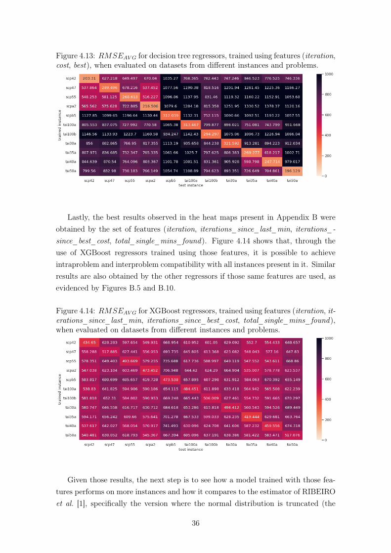
Figure 4.13: RMSEAV G for decision tree regressors, trained using features (iteration,cost, best), when evaluated on datasets from different instances and problems.
Lastly, the best results observed in the heat maps present in Appendix B wereobtained by the set of features (iteration, iterations_since_last_min, iterations_-since_best_cost, total_single_mins_found). Figure 4.14 shows that, through theuse of XGBoost regressors trained using those features, it is possible to achieveintraproblem and interproblem compatibility with all instances present in it. Similarresults are also obtained by the other regressors if those same features are used, asevidenced by Figures B.5 and B.10.
Figure 4.14: RMSEAV G for XGBoost regressors, trained using features (iteration, it-erations_since_last_min, iterations_since_best_cost, total_single_mins_found),when evaluated on datasets from different instances and problems.
Given those results, the next step is to see how a model trained with those fea-tures performs on more instances and how it compares to the estimator of RIBEIROet al. [1], specifically the version where the normal distribution is truncated (the
36

boundaries available are covered in Section 3.2.3). However, It is importance tonote that, because of the differences in methodology mentioned in Section 3.2, thetwo techniques might not be directly comparable and, for that reason, any compar-ison present in this chapter should be taken cautiously.
With that said, in order to see how they perform, 20 instances were picked,where each problem was represented by 10 and each instance was composed of 10executions of 1 000 000 iterations. As for the model, the XGBoost regressor trainedon the instance scp42 unsing the features (iteration, iterations_since_last_min,iterations_since_best_cost, total_single_mins_found) was chosen. The results arepresented in Table 4.1.
InstanceRMSEAV G
Prob. Stop.RMSEAV G
ML Stop.
scp42 1183.977 685.566scp49 878.609 568.823scp51 1039.964 564.044scp65 1805.396 701.463scp410 979.393 937.042scpa4 828.858 664.459scpb3 3509.505 547.835scpc1 789.983 786.967scpd1 3209.535 793.654scpd5 3020.280 706.606
InstanceRMSEAV G
Prob. Stop.RMSEAV G
ML Stop.
bur26d 444.061 3629.979chr22a 941.914 1363.105esc16j 1661.684 147175.093had12 321.235 59845.361lipa20a 562.791 6869.520nug12 486.695 9922.096rou20 385.643 960.119sko56 802.080 805.096tai30a 493.438 701.353wil50 1532.034 649.188
Table 4.1: Error RMSEAV G for the XGboost model trained on scp42 instances usingfeatures (iteration, iterations_since_last_min, iterations_since_best_cost, total_-single_mins_found).
The values shown in that table demonstrate that the selected model performswell on SCP instances, achieving a RMSEAV G smaller than the ones obtained fromthe estimates provided by the estimator of RIBEIRO et al. [1]. On the other hand,when the results for the QAP instances are observed, it is possible to see that theregressor lost in many instances and even performed very poorly in some.
When the reasons for the bad performance on instances bur26d, chr22a, esc16j,had12, lipa20a and nug12 are investigated, the first relevant information to be givenis related to the method used to obtain those numbers, that was different for eachproblem. For the SCP instances, the estimates were calculated (1) at the firstiteration, (2) at every time the best solution changed, and also (3) at every 50
iterations. Meanwhile, for the QAP instances, the calculation only happened in thefirst two situations.
That difference was motivated by the fact that, for the QAP problem, the estima-tor of RIBEIRO et al. [1] can take several minutes to calculate the CDF, while it cantake up to a little more than a second to do the same for the SCP instances. Thatslowness is caused, among other factors, by the huge distances between the bound-
37

aries of some QAP instances, that are taken into account during the calculation ofthe integral.
It is also important to mention that, for the executions of the instances presentin the table, the calculation of the RMSE for a single execution was performed overall iterations it has. To make that possible, iterations where the estimators werenot executed received the estimates obtained at the last prior iteration where theywere.
The second relevant information to be considered are the characteristics of theinstances. In the case of the esc16j, the optimal solution is usually found in thefirst 10 iterations, while in bur26d, had12, lipa20a and nug12 it appears within thefirst few hundred iterations. While this kind of event might be identified by modelsthat take into account cost value, the same does not apply to the model employed,because it does not know the cost obtained at a given iteration and was trained onan instance where the solution is gradually improved over time.
Given that situation, if the XGBoost regressor is replaced by a model trained ona set of features that is aware of cost value, there might be room for improvement.In Table 4.2, the results obtained from a decision tree regressor trained on a scp42instance using the features (iteration, cost, best) are presented.
InstanceRMSEAV G
Prob. Stop.RMSEAV G
ML Stop.
scp42 1183.977 602.545scp49 878.609 690.485scp51 1039.964 361.297scp65 1805.396 598.271scp410 979.393 525.995scpa4 828.858 358.393scpb3 3509.505 755.885scpc1 789.983 306.965scpd1 3209.535 575.697scpd5 3020.280 638.862
InstanceRMSEAV G
Prob. Stop.RMSEAV G
ML Stop.
bur26d 444.061 1320.345chr22a 941.914 640.586esc16j 1661.684 38659.235had12 321.235 13044.678lipa20a 562.791 2699.114nug12 486.695 10667.865rou20 385.643 595.476sko56 802.080 566.802tai30a 493.438 888.368wil50 1532.034 810.466
Table 4.2: Error RMSEAV G for the Decision Tree Regressor model trained on scp42instances using features (iteration, cost, best).
Comparing those results to the ones shown in Table 4.2, it is possible to see thatthe use of the cost-aware features improved the results for many instances (while alsoincreasing the error on a few others, but not by a very significant amount), resultingin a smaller error than the cost-unaware model, that, according to Figure 4.14,appeared to have better generalization capabilities. It also increased the numberof situations where the machine learning model obtains a smaller error than theCDF-based estimator. Nonetheless, the errors continue to be high for the instancesbur26d, esc16j, had12, lipa20a and nug12, and one of the few ways to reduce it
38

further, without resorting to problem-specific models (like one trained on an easyQAP instance), may be through the production of estimates at fixed intervals, likewhat was done for the SCP instances.
In Table B.1, that approach is evaluated and validated on an extensive groupof instances, where it can be seen that, by estimating the probability regularly, theerror can be reduced. In that table, the models marked by (ii) produced estimatesat the first iteration, every time the minimum changed and at every 50 iterations,while the estimators accompanied by a (i) were run in the first two situations.
In addition to the models used in Tables 4.1 and 4.2, Table B.1 also includesresults for two tai100a estimators that were trained on the same feature sets usedby the scp42 models. However, despite the fact that those estimators also showedpositive results when the probability is evaluated regularly, they did not seem tobring any relevant advantage when compared to their scp42 counterparts (even onQAP instances), but it is important to note that the tai100a is not an easy instanceand, unlike the esc16j or the bur26d, the optimal solution is not expected to befound after just a handful of iterations.
It is also possible to see that not all instances were represented by 10 execu-tions. That happened because some executions experienced errors while runningthe estimator of RIBEIRO et al. [1] (in most cases, it appeared to be some kind ofvariable overflow) or while running GRASP (in few occasions, the program appar-ently crashed before reaching one million iterations). In some cases, that kind ofproblem also impeded the use of all executions of an instance. For instances esc16b,esc16f, esc16h, esc16i, esc32e and esc32g, all executions experienced errors (the onethat appears to be a variable overflow) and, for that reason, their respective resultswere not included. Some instances were also removed due to their difficulty. Specif-ically, instances tai150b, tai256c and tho150 were initially considered and some oftheir executions were started, but, due to the long time required to reach one millioniterations, they were discarded.
With that said, in Table 4.3, a comparison between the CDF based estimatorand the machine learning models is provided, based on the data available in TableB.1. In that table, the SCP problem is represented by 45 instances, while the QAPis represented by 125. It is possible to observe that, for a XGBoost regressor, trainedon instance scp42, using features (iteration, iterations_since_last_min, iterations_-since_best_cost, total_single_mins_found), it is possible to obtain a smaller errorthan the estimator of RIBEIRO et al. [1] in more than 50% of the instances, inboth problems. But that only happens if the estimates are produced at every 50
iterations and are compared to the CDF being executed only at iterations wherethere is a change in minimum. If both techniques produce estimates only duringminimum changes, the machine learning models still show better results on SCP
39

instances, but perform worse than the CDF in QAP instances. In any case, it isimportant to note that those results must be taken cautiously, given the differencein methodology (mentioned in Chapter 3) between the present work and the workof RIBEIRO et al. [1].
model momentestimation
(all inst.)smaller error
% model
(SCP inst.)smaller error
% model
(QAP inst.)smaller error
% model
XGB_E_scp42 (i) 40.0 84.4 24.0XGB_E_scp42 (ii) 68.8 100.0 57.6DTR_C_scp42 (i) 40.6 93.3 21.6DTR_C_scp42 (ii) 58.2 100.0 43.2
XGB_E_tai100a (i) 33.5 84.4 15.2XGB_E_tai100a (ii) 65.9 100.0 53.6RFR_C_tai100a (i) 44.1 100.0 24.0RFR_C_tai100a (ii) 59.4 100.0 44.8
Table 4.3: Comparison between the CDF-based estimator and four machine learningmodels when evaluating 170 different instances (45 SCP and 125 QAP). In all cases,the CDF-based estimator was only executed in the first iteration of an executionand during minimum changes.
Another important aspect to be evaluated in this work is the time an estimatortakes to output a value. In Table C.1, the average times obtained while running theinstances presented in Tables 4.1 and 4.2 are presented. Based on those results, it ispossible to argue that the machine learning based approach can be faster than theCDF-based estimator. However, the time taken depends on the machine learningtechnique being utilized. When the times observed for the XGBoost regressor arecompared to those observed for the decision tree regressor, the latter proves be muchfaster than the former, and that is caused by the fact that a decision tree regressoris much simpler than a XGBosst regressor, as shown in Sections 2.2.1 and 2.2.3.
Lastly, in Table C.2 the stopping rule is evaluated. Specifically, it is observed atwhich iteration executions of the instances present in Table C.1 would stop, givena threshold β. In those results, it is possible to observe, in a more practical way,how well the XGBoost regressor and the decision tree regressor perform on SCP andQAP instances. It corroborates, for example, with the argument that the machinelearning models utilized have a bad performance on easy QAP instances and that theestimation of the probabilities at fixed intervals could have improved that situations.
4.4 Model Choice
In this work, a total of 165 models were generated and utilized for testing purposes.Most of them were only applied to a limited set of unknown instances, while a few
40

others were used to make predictions for many more. In that universe of models,they varied on instance used for training, machine learning technique and featureset, and that leads to one question: which one should be used?
The answer for such a question is not simple. Considering the results obtainedin this work, two feature sets showed relevant generalization capabilities. They are(iteration, cost, best) and (iteration, iterations_since_last_min, iterations_since_-best_cost, total_single_mins_found). However, the features are only part of thedecision process. The machine learning technique and the parameters used by themare also of utmost importance. To exemplify that, the results obtained by theXGBoost regressor for most feature combination can be used. The technique itselfis expected to be more powerful than decision tree regression and random forestregression. Nonetheless, it achieved bad results in many scenarios because of anapparently poor parameter selection.
Based on those facts, the recommendations made by this work are not limitedto a single model, technique, etc. If simplicity and very fast training speeds areimportant, decision tree regression has shown to be as usable as the other twotechniques. On the other hand, if less risk of over fitting is desired, random forestregression and XGBoost might be a good choices.
Additionally, as mentioned earlier, two feature sets showed relevant results. How-ever, instead of considering only one of them, the use of both might be a betterchoice, because one showed better results on some instances, while the other wasbetter on others. In that case, two models could be used, forming an ensemble whereeach of its components would be trained using a different feature set. The output,in that case, could be the average or the smallest probability estimated among themodels.
When it comes to which instance should be used for training, it depends onthe target problem and instance. In the context of this work, models trained on ascp42 showed good results when used to evaluate other SCP instances, but faced aless favorable scenario in QAP instances, having a bad performance on easy ones.In those cases, the models would eventually stop the execution at some point, butpossibly at a greater cost than the required by the estimator of RIBEIRO et al. [1].
41

Chapter 5
Conclusions
This chapter closes this text by presenting the final remarks and a series of possiblepaths to be followed from the point where this work stopped.
5.1 Final Remarks
In this work, it was shown that machine learning can be used to replace the roleperformed by the CDF in the probabilistic stopping rule for the GRASP metaheuris-tic. With the approach taken, it was possible to achieve a better performance onmany of the instances tested, and that happened for the time required to evaluatean iteration and for the error obtained by the estimates when they are compared tothe expected values within sufficiently large executions (large samples).
Moreover, the method also demonstrated generalization capabilities, where somemodels trained on a given instance of a given problem were able to provide relevantestimates for executions from instances belonging to the same problem and to otherproblems. The key in this case resides in the features used by the models. For ex-ample, models unaware of cost value might be able to generalize to more instances,while models trained on features that include cost value might produce better es-timates on situations where the global minimum — or a very good local minimum— is found early in an execution, because that feature is able to express, indirectly,that the optimal solution (or a very good one) was indeed found.
The main drawback of the proposed technique, on the other hand, is the needto train a model before using it, which involves two time consuming activities. Thefirst is data acquisition, that requires the accumulation of large executions of a giveninstance, and the second is the act of training the model on that data. Model trainingis usually the fastest part among the two. However, how long it takes depends onthe machine learning technique being used.
In order to mitigate that, in this work, it was shown that tree-based models werefast to train, making the time required for that relatively negligible. As for the time
42

required to obtain the training data, it still represents the main disadvantage ofwhat is proposed in this work when compared to the stopping rule using CDF, thatcan work with any standard GRASP optimization without needing prior procedures.However, if the model proves to be able to generalize to the instances it is intendedto be applied, the training will be a one-time activity.
Finally, it is possible to conclude that a machine learning based probabilisticstopping criterion for GRASP is feasible and effective, performing better than theoriginal probabilistic stopping rule in many situations. But that comes at costin time prior to its use that must be must be taken into consideration by thoseintending to use it. For that reason, the observations that can be made are thatthe stopping rule of RIBEIRO et al. [1] is more appropriate to situations wherethe time required to apply the method proposed in this work is not available andguaranteed generalization is needed, while the machine learning-based approach ismore suitable to cases where the estimates are expected to be produced repeatedlyin a short period of time.
5.2 Future Works
In order to expand the current work and possibly improve its results, six additionalapproaches are intended to be evaluated. The first is to verify the impact of aligningthe methodology of the proposed technique to what is done by the stopping rule ofRIBEIRO et al. [1] to calculate the number of future minimums. In this case,datasets of 2 000 000 iterations could be used, where iterations from 1 000 001 to2 000 000 would be employed exclusively for that purpose, allowing the observationof 1 000 000 iterations in the future for any of the first 1 000 000 iterations.
As for the second future work, it would be checking the impact of tighteningthe boundaries of the instances. The upper bounds used in the present work werevery loose and far from what was effectively observed in the executions, a fact thatalso contributed to the high times observed during the execution of the stoppingcriterion of RIBEIRO et al. [1] on QAP instances.
The third open possibility is to seek for ideal sizes for the dataset. The oneemployed in this work was based on limited tests and it might be possible to achievesimilar results with datasets that are smaller (in number of executions or in numberof iterations per execution).
The fourth possible approach is to check if online learning can be used somehow.The application of a machine learning technique of that kind could happen in com-bination with a traditional stopping criterion, like a limited number of iterations ortime, where it could take over the decision process on whether to stop the search ornot once it starts producing results as good as the other criteria. Similarly, the model
43

could also be combined with the original probabilistic stopping rule and trained onits estimates. In these cases, the model might not produced better estimates, butmight achieve results that are comparable to the other technique in a faster way.
The fifth loose end is the application of the method on other problems. InRIBEIRO et al. [1], four problems were used to test the technique they proposed,while, in this work, only two were employed. Testing the machine learning basedapproach on more problems would allow the identification of eventual additionallimitations to its generalization capability.
The sixth - and last - thing that is intended to be evaluated in the future is theuse of additional features and additional combinations of them. In this work, forexample, cost autocorrelation and features derived from cost history (like average,variance and standard deviation) were not considered, but could produce relevantresults.
44

References
[1] RIBEIRO, C. C., ROSSETI, I., SOUZA, R. C. “Probabilistic stopping rules forGRASP heuristics and extensions”, International Transactions in Opera-tional Research, v. 20, n. 3, pp. 301–323, 2013. doi: https://doi.org/10.1111/itor.12010. Disponível em: <https://onlinelibrary.wiley.com/
doi/abs/10.1111/itor.12010>.
[2] FEO, T. A.AND RESENDE, M. G. C. “Greedy Randomized Adaptive SearchProcedures”, Journal of Global Optimization, v. 6, n. 2, pp. 109–133,Mar 1995. ISSN: 1573-2916. doi: 10.1007/BF01096763. Disponível em:<https://doi.org/10.1007/BF01096763>.
[3] QUINLAN, J. R. “Induction of decision trees”, Machine Learning, v. 1, n. 1,pp. 81–106, Mar 1986. ISSN: 1573-0565. doi: 10.1007/BF00116251.Disponível em: <https://doi.org/10.1007/BF00116251>.
[4] QUINLAN, J. R. C4.5: Programs for Machine Learning. San Mateo, CA,Morgan Kaufmann, 1993. ISBN: 1-55860-238-0.
[5] LOH, W.-Y. “Fifty Years of Classification and Regression Trees”, InternationalStatistical Review, v. 82, n. 3, pp. 329–348, 2014. doi: https://doi.org/10.1111/insr.12016. Disponível em: <https://onlinelibrary.wiley.
com/doi/abs/10.1111/insr.12016>.
[6] MORGAN, J. N., SONQUIST, J. A. “Problems in the Analysis of Survey Data,and a Proposal”, Journal of the American Statistical Association, v. 58,n. 302, pp. 415–434, 1963. ISSN: 01621459. doi: https://doi.org/10.2307/2283276. Disponível em: <http://www.jstor.org/stable/2283276>.
[7] BREIMAN, L., FRIEDMAN, J. H., OLSHEN, R. A., et al. Classification AndRegression Trees. 1 ed. Boca Raton, Chapman and Hall/CRC, 1984.ISBN: 0-412-04841-8.
[8] BREIMAN, L. “Random Forests”, Machine Learning, v. 45, n. 1, pp. 5–32, Oct2001. ISSN: 1573-0565. doi: 10.1023/A:1010933404324. Disponível em:<https://doi.org/10.1023/A:1010933404324>.
45

[9] CHEN, T., GUESTRIN, C. “XGBoost: A Scalable Tree Boosting System”.In: Proceedings of the 22nd ACM SIGKDD International Conferenceon Knowledge Discovery and Data Mining, KDD ’16, p. 785–794, NewYork, NY, USA, 2016. Association for Computing Machinery. ISBN:9781450342322. doi: 10.1145/2939672.2939785. Disponível em: <https:
//doi.org/10.1145/2939672.2939785>.
[10] FRIEDMAN, J. H. “Greedy Function Approximation: A Gradient BoostingMachine”, The Annals of Statistics, v. 29, n. 5, pp. 1189–1232, 2001. ISSN:00905364. Disponível em: <http://www.jstor.org/stable/2699986>.
[11] NIELSEN, D. “Tree boosting with XGBoost - why does XGBoost win "Every"machine learning competition?” Dec 2016. Disponível em: <http://
hdl.handle.net/11250/2433761>.
[12] KORTE, B., VYGEN, J. “Approximation Algorithms”. In: CombinatorialOptimization: Theory and Algorithms, pp. 413–457, Berlin, Heidel-berg, Springer Berlin Heidelberg, 2012. ISBN: 978-3-642-24488-9. doi:10.1007/978-3-642-24488-9_16. Disponível em: <https://doi.org/10.
1007/978-3-642-24488-9_16>.
[13] VAZIRANI, V. V. Approximation Algorithms. Springer Berlin Heidelberg,2003. doi: 10.1007/978-3-662-04565-7. Disponível em: <https://doi.
org/10.1007/978-3-662-04565-7>.
[14] PESSOA, L. S., RESENDE, M. G. C., RIBEIRO, C. C. “A Hybrid LagrangeanHeuristic with GRASP and Path-Relinking for Set k-Covering”, Comput.Oper. Res., v. 40, n. 12, pp. 3132–3146, dez. 2013. ISSN: 0305-0548. doi:10.1016/j.cor.2011.11.018. Disponível em: <https://doi.org/10.1016/
j.cor.2011.11.018>.
[15] KOOPMANS, T. C., BECKMANN, M. J. “Assignment Problems and theLocation of Economic Activities”, Econometrica, v. 25, n. 1, pp. 53–76,1957. ISSN: 00129682, 14680262. Disponível em: <http://www.jstor.
org/stable/1907742>.
[16] SAHNI, S., GONZALEZ, T. “P-Complete Approximation Problems”, J. ACM,v. 23, n. 3, pp. 555–565, jul. 1976. ISSN: 0004-5411. doi: 10.1145/321958.321975. Disponível em: <https://doi.org/10.1145/321958.321975>.
[17] OLIVEIRA, C. A. S., PARDALOS, P. M., RESENDE, M. G. C. “GRASPwith Path-Relinking for the Quadratic Assignment Problem”. In: Ribeiro,C. C., Martins, S. L. (Eds.), Experimental and Efficient Algorithms, pp.
46

356–368, Berlin, Heidelberg, 2004. Springer Berlin Heidelberg. ISBN: 978-3-540-24838-5.
[18] BEASLEY, J. E. “OR-Library: Distributing Test Problems by Electronic Mail”,The Journal of the Operational Research Society, v. 41, n. 11, pp. 1069–1072, 1990. ISSN: 01605682, 14769360. Disponível em: <http://www.
jstor.org/stable/2582903>.
[19] BURKARD, R. E.AND KARISCH, S. E., RENDL, F. “QAPLIB – A QuadraticAssignment Problem Library”, Journal of Global Optimization, v. 10, n. 4,pp. 391–403, Jun 1997. ISSN: 1573-2916. doi: 10.1023/A:1008293323270.Disponível em: <https://doi.org/10.1023/A:1008293323270>.
[20] “’auto’ value of max_features for RandomForestRegressor is poor”. https://github.com/scikit-learn/scikit-learn/issues/7254, 2016. [Online;accessed 31-August-2021].
[21] “Ensemble Methods”. https://scikit-learn.org/stable/modules/
ensemble.html#parameters. [Online; accessed 31-August-2021].
[22] RASHMI, K. V., GILAD-BACHRACH, R. “DART: Dropouts meet MultipleAdditive Regression Trees”. 2015.
47

Appendix A
Instance’s Lower and Upper Bounds
Instance LB UB Instance LB UB
scp41 1148 37742 scp64 292 39068scp410 1356 37151 scp65 353 39155scp42 1205 37132 scpa1 562 58870scp43 1213 37221 scpa2 560 58550scp44 1185 37145 scpa3 524 58771scp45 1266 37271 scpa4 527 58751scp46 1349 37239 scpa5 557 58754scp47 1115 36570 scpb1 149 59578scp48 1225 37276 scpb2 150 59554scp49 1485 37221 scpb3 165 59585scp51 579 39087 scpb4 157 59740scp510 672 38823 scpb5 151 59676scp52 677 38818 scpc1 514 79004scp53 574 38776 scpc2 483 79028scp54 582 38736 scpc3 544 78796scp55 550 38972 scpc4 484 78793scp56 560 38911 scpc5 488 78697scp57 695 38690 scpd1 122 79771scp58 662 38341 scpd2 127 79714scp59 687 38610 scpd3 138 79783scp61 283 39344 scpd4 122 79520scp62 302 38938 scpd5 130 79672scp63 313 38895
Table A.1: SCP instances and their respective lower and upper bounds.
48

Instance LB UB Instance LB UB Instance LB UB
bur26a 5426670 100245444 had18 5358 25056 sko100d 141289 1584000bur26b 3817852 67331030 had20 6922 34280 sko100e 140893 1584000bur26c 5426795 83306912 kra30a 88900 1326000 sko100f 140691 1584000bur26d 3821225 55973502 kra30b 91420 1362000 sko42 14934 168840bur26e 5386879 93811198 kra32 88700 1546240 sko49 22004 251860bur26f 3782044 63025638 lipa20a 3683 14360 sko56 32610 358400bur26g 10117172 187561244 lipa20b 27076 138400 sko64 45736 504320bur26h 7098658 125978580 lipa30a 13178 50400 sko72 62691 682560chr12a 9552 867240 lipa30b 151426 739620 sko81 86072 920970chr12b 9742 867240 lipa40a 31538 118720 sko90 109030 1209600chr12c 11156 867240 lipa40b 476581 2340240 ste36a 9526 862056chr15a 9896 1529310 lipa50a 62093 234500 ste36b 15852 5799600chr15b 7990 1529310 lipa50b 1210244 5801600 ste36c 8239110 700694568chr15c 9504 1529310 lipa60a 107218 404940 tai100a 15844731 97714200chr18a 11098 2212164 lipa60b 2520135 12043080 tai100b 1058131796 130115042000chr18b 1534 140616 lipa70a 169755 650650 tai12a 224416 1256808chr20a 2192 283320 lipa70b 4603200 22604400 tai12b 39464925 1757709624chr20b 2298 283320 lipa80a 253195 970400 tai150b 441786736 26078235600chr20c 14142 3021520 lipa80b 7763962 38504960 tai15a 388214 1935390chr22a 6156 791604 lipa90a 360630 1395000 tai15b 51765268 12248023585chr22b 6194 791604 lipa90b 12490441 62360910 tai17a 491812 2552635chr25a 3796 1055650 nug12 578 5856 tai20a 703482 3626400els19 17212548 1704030732 nug14 1014 10080 tai20b 122455319 13048373980
esc128 64 96768 nug15 1150 11850 tai256c 43849646 6553600000esc16a 68 1632 nug16a 1610 14720 tai25a 1167256 5883300esc16b 292 1728 nug16b 1240 13440 tai25b 344355646 28051179500esc16c 160 2688 nug17 1732 16830 tai30a 1706855 8596620esc16d 16 960 nug18 1930 18720 tai30b 637117113 42004266660esc16e 28 1344 nug20 2570 24800 tai35a 2216627 11803330esc16f 0 0 nug21 2438 31500 tai35b 242172800 20629796495esc16g 26 1536 nug22 3596 47960 tai40a 2843274 15469120esc16h 996 16128 nug24 3488 40320 tai40b 564428353 34766639600esc16i 14 1632 nug25 3744 43500 tai50a 4390920 24275700esc16j 8 864 nug27 5234 64800 tai50b 395543467 30319229200esc32a 130 13568 nug28 5166 61600 tai60a 5578356 34999680esc32b 168 8192 nug30 6124 70200 tai60b 542376603 49191714900esc32c 642 16896 rou12 235528 1290840 tai64c 1855928 409600000esc32d 200 8704 rou15 354210 2053350 tai80a 10501941 62394560esc32e 2 4096 rou20 725522 3714560 tai80b 717907288 65951742240esc32g 6 3584 scr12 31410 961560 tho150 8133398 114180600esc32h 438 11776 scr15 51140 1858350 tho30 149936 2101860esc64a 116 22400 scr20 110030 4897200 tho40 240516 3730400had12 1652 7320 sko100a 143846 1584000 wil100 273038 1425600had14 2724 13216 sko100b 145522 1584000 wil50 48816 258300had16 3720 17408 sko100c 139881 1584000
Table A.2: QAP instances and their respective lower and upper bounds.
49

Appendix B
Error Heatmaps and Error Tables
Figure B.1: RMSEAV G for decision tree regressors, trained using features (best_-cost, best), when evaluated on datasets from different instances and problems.
50

Figure B.2: RMSEAV G for decision tree regressors, trained using features (iteration,cost, best_cost), when evaluated on datasets from different instances and problems.
Figure B.3: RMSEAV G for decision tree regressors, trained using features (iteration,cost, best), when evaluated on datasets from different instances and problems.
51

Figure B.4: RMSEAV G for decision tree regressors, trained using features (itera-tion, cost, best_cost, best), when evaluated on datasets from different instances andproblems.
Figure B.5: RMSEAV G for decision tree regressors, trained using features (itera-tion, iterations_since_last_min, iterations_since_best_cost, total_single_mins_-found), when evaluated on datasets from different instances and problems.
52

Figure B.6: RMSEAV G for random forest regressors, trained using features (best_-cost, best), when evaluated on datasets from different instances and problems.
Figure B.7: RMSEAV G for random forest regressors, trained using features (iter-ation, cost, best_cost), when evaluated on datasets from different instances andproblems.
53

Figure B.8: RMSEAV G for random forest regressors, trained using features (itera-tion, cost, best), when evaluated on datasets from different instances and problems.
Figure B.9: RMSEAV G for random forest regressors, trained using features (itera-tion, cost, best_cost, best), when evaluated on datasets from different instances andproblems.
54

Figure B.10: RMSEAV G for random forest regressors, trained using features (itera-tion, iterations_since_last_min, iterations_since_best_cost, total_single_mins_-found), when evaluated on datasets from different instances and problems.
Figure B.11: RMSEAV G for XGBoost regressors, trained using features (best_cost,best), when evaluated on datasets from different instances and problems.
55

Figure B.12: RMSEAV G for XGBoost regressors, trained using features (iteration,cost, best_cost), when evaluated on datasets from different instances and problems.
Figure B.13: RMSEAV G for XGBoost regressors, trained using features (iteration,cost, best), when evaluated on datasets from different instances and problems.
56

Figure B.14: RMSEAV G for XGBoost regressors, trained using features (iteration,cost, best_cost, best), when evaluated on datasets from different instances and prob-lems.
Figure B.15: RMSEAV G for XGBoost regressors, trained using features (itera-tion, iterations_since_last_min, iterations_since_best_cost, total_single_mins_-found), when evaluated on datasets from different instances and problems.
57

Table B.1: RMSEAV G observed for the probabilistic stoppingrule of RIBEIRO et al. [1] and for different machine learningmodels when applied to multiple SCP and QAP instances. (i)are results obtained when the estimators are executed only inthe first iteration and on changes of minimum cost, while in(ii) the estimators are also executed at every 50 iterations.Feature set codes come from Table 3.6.
Instance(Execs.)Num.
(i)StopProb.
(i)scp42
EXGB
(ii)scp42
EXGB
(i)scp42
CDTR
(ii)scp42
CDTR
(i)tai100a
EXGB
(ii)tai100a
EXGB
(i)tai100a
CRFR
(ii)tai100a
CRFR
bur26a.dat 10 580.4 6296.1 627.4 3721.1 785.9 5615.0 632.3 5618.2 765.1bur26b.dat 10 511.1 1839.0 793.8 1200.3 620.1 2871.7 573.3 1705.4 614.8bur26c.dat 10 621.6 6940.1 683.2 3815.7 836.8 1525.7 741.2 4204.6 812.8bur26d.dat 10 522.3 3133.8 665.1 2003.3 649.6 2071.1 570.6 3901.2 625.8bur26e.dat 10 582.4 2728.1 565.7 1486.3 732.0 2044.7 706.8 1497.5 711.0bur26f.dat 10 570.1 10173.5 452.3 5666.6 695.4 7623.8 549.4 5481.0 676.0bur26g.dat 10 723.0 2084.3 726.3 2310.4 873.5 2046.4 687.0 1500.9 862.6bur26h.dat 10 401.6 3549.2 540.6 2186.8 551.3 2405.7 442.9 4444.8 530.2chr12a.dat 10 380.2 10719.4 498.7 5964.0 498.1 1937.7 521.6 7524.4 518.6chr12b.dat 10 466.6 18423.1 775.4 11132.1 647.5 45341.9 647.6 18090.6 712.2chr12c.dat 10 394.1 2195.1 401.0 1665.9 606.7 1651.4 443.3 2028.3 619.5chr15a.dat 10 434.5 561.4 640.2 896.6 520.9 1768.3 535.9 1251.6 489.8chr15b.dat 10 812.9 7595.9 737.1 3989.7 898.9 1292.5 777.7 4516.4 876.7chr15c.dat 10 731.9 796.2 689.4 1563.1 725.7 1591.2 714.1 1582.3 717.7chr18a.dat 10 498.5 826.0 474.2 910.4 755.4 862.3 507.7 1312.6 736.0chr18b.dat 10 615.1 544.5 556.3 1691.2 543.4 21887.1 784.3 6018.5 526.0chr20a.dat 10 758.5 902.1 691.2 887.2 847.9 902.1 694.5 1747.0 835.2chr20b.dat 10 1172.2 892.7 600.1 1045.5 968.7 1055.3 649.3 1012.1 952.1chr20c.dat 10 397.8 2282.1 439.4 1844.5 379.3 429.1 400.6 1105.4 356.8chr22a.dat 10 765.9 914.2 693.9 722.6 730.8 714.1 582.8 713.6 708.7chr22b.dat 9 675.2 647.5 491.1 607.1 613.0 782.7 477.2 576.3 584.8chr25a.dat 10 661.5 963.1 615.3 803.4 783.5 785.4 636.5 816.2 762.7els19.dat 10 947.5 10962.8 592.0 3456.3 517.1 16563.1 719.3 6260.3 482.7
esc128.dat 10 285.3 31618.0 408.4 6310.5 469.6 4860.6 545.6 9310.5 453.0esc16a.dat 8 1244.5 244.0 753.6 29284.2 307.5 242317.2 964.7 21699.2 320.6esc16c.dat 7 1063.1 90.8 677.6 38658.6 169.7 231606.6 867.1 25915.2 193.1esc16d.dat 6 2016.7 0.0 687.3 38658.0 104.4 203941.7 615.6 24457.0 124.5esc16e.dat 8 1591.3 69655.4 824.5 38658.4 161.2 169219.2 745.9 27007.9 184.6esc16g.dat 9 1716.4 139621.2 806.2 34477.5 243.8 164843.3 830.3 26369.6 265.0esc16j.dat 10 1777.8 91.5 696.5 34903.5 175.7 30881.5 1079.3 25469.2 198.6
58

Instance(Execs.)Num.
(i)StopProb.
(i)scp42
EXGB
(ii)scp42
EXGB
(i)scp42
CDTR
(ii)scp42
CDTR
(i)tai100a
EXGB
(ii)tai100a
EXGB
(i)tai100a
CRFR
(ii)tai100a
CRFR
esc32a.dat 9 439.5 636.0 421.4 571.4 591.3 771.1 497.3 561.7 563.1esc32b.dat 9 562.4 728.3 585.7 8984.9 347.1 27404.2 553.7 8287.3 334.6esc32c.dat 6 1134.5 562.3 998.6 26263.6 589.5 158391.3 844.6 26705.6 600.8esc32d.dat 10 305.2 3190.3 614.7 16571.1 448.3 75075.8 562.9 18854.2 446.4esc32h.dat 9 380.4 11004.0 730.6 3171.2 340.9 7636.9 537.9 5275.0 323.0esc64a.dat 5 2078.6 106303.5 856.8 38659.0 203.5 225889.1 888.4 25875.2 226.8had12.dat 10 316.2 12338.7 500.8 3307.3 451.1 29262.3 451.0 11994.9 510.1had14.dat 10 396.2 9894.1 512.4 35483.0 574.2 97662.7 650.7 17815.5 554.6had16.dat 10 316.4 392.4 631.6 12181.2 422.3 114064.4 632.7 13871.9 382.5had18.dat 10 355.5 16989.3 452.2 14757.2 616.4 13957.2 572.6 12868.4 607.0had20.dat 10 446.3 6792.3 464.5 9435.8 657.3 11922.2 515.1 12409.4 650.3kra30a.dat 10 850.4 1095.7 723.9 1474.1 585.8 952.1 583.8 1234.9 606.6kra30b.dat 10 549.6 816.2 456.3 501.7 444.2 994.8 534.6 461.6 422.7kra32.dat 10 593.0 854.8 496.3 1063.7 686.7 726.5 590.0 3008.6 665.5
lipa20a.dat 10 706.0 2802.9 534.4 7680.4 520.6 13434.9 654.5 6385.5 554.7lipa20b.dat 10 414.2 24685.0 665.6 16577.0 523.9 66488.5 589.8 21588.0 692.3lipa30a.dat 10 522.5 679.2 590.0 1611.3 581.3 1625.0 513.1 1150.2 608.6lipa30b.dat 10 302.6 7429.1 521.7 10916.9 454.6 66177.6 487.3 15762.1 523.9lipa40a.dat 10 609.8 605.4 565.9 623.6 626.1 847.3 557.2 608.9 620.5lipa40b.dat 10 448.8 33470.7 516.6 37984.5 564.6 18189.8 617.1 10895.5 586.4lipa50a.dat 10 563.8 603.3 537.9 647.3 654.2 641.9 560.1 680.1 647.9lipa50b.dat 10 557.0 7624.8 626.1 3527.8 561.6 3946.5 606.4 3667.7 670.7lipa60a.dat 10 513.3 863.0 509.6 1139.5 622.3 1158.0 496.3 1156.2 605.9lipa60b.dat 10 335.1 4686.4 413.5 1368.0 583.8 10010.3 476.2 4383.7 503.8lipa70a.dat 10 543.5 796.6 594.2 825.2 858.8 925.5 661.0 889.3 830.1lipa70b.dat 10 641.0 4187.1 535.2 2606.0 591.7 9392.4 594.5 3582.4 571.7lipa80a.dat 10 710.5 592.7 550.5 601.7 556.6 586.2 571.7 597.8 543.4lipa80b.dat 10 509.1 821.3 589.8 1462.6 659.7 1509.5 625.9 1366.0 761.2lipa90a.dat 10 701.7 833.0 621.0 782.7 795.3 957.5 679.7 759.5 764.4lipa90b.dat 10 653.3 613.4 621.4 4524.5 575.7 2594.8 631.8 2389.0 545.3nug12.dat 10 543.3 14305.4 689.0 7631.5 799.8 6292.9 636.0 8369.4 812.6nug14.dat 10 406.8 3923.6 580.4 2501.1 652.6 2160.5 536.2 3074.7 702.8nug15.dat 10 402.6 23567.3 556.7 3701.7 689.1 19548.3 531.2 11221.6 692.6nug16a.dat 10 462.0 3890.4 412.4 1410.7 526.0 12041.1 478.1 2150.0 528.4nug16b.dat 10 401.6 37224.7 449.3 7763.2 523.0 47965.9 647.7 14214.3 525.6nug17.dat 10 551.8 1110.0 579.6 912.4 552.2 2433.0 663.1 1194.3 529.7nug18.dat 10 417.5 618.0 478.0 5656.4 552.4 19568.3 507.5 4795.1 554.8
59

Instance(Execs.)Num.
(i)StopProb.
(i)scp42
EXGB
(ii)scp42
EXGB
(i)scp42
CDTR
(ii)scp42
CDTR
(i)tai100a
EXGB
(ii)tai100a
EXGB
(i)tai100a
CRFR
(ii)tai100a
CRFR
nug20.dat 10 393.8 588.3 542.2 1265.7 529.5 4026.2 514.7 1497.0 510.9nug21.dat 9 495.6 720.5 481.4 963.9 655.2 14835.7 537.3 995.6 645.9nug22.dat 10 410.2 1517.4 656.0 1594.9 627.4 2766.9 534.4 3125.0 626.2nug24.dat 10 442.2 4435.4 448.5 1870.7 667.3 1800.7 497.5 2035.6 662.1nug25.dat 10 667.7 2574.8 700.3 1749.8 965.6 1068.1 665.1 1407.7 951.7nug27.dat 10 800.8 1233.1 768.1 1767.5 715.9 2018.1 737.9 1523.9 699.7nug28.dat 9 606.3 986.2 539.9 1319.2 743.4 931.6 568.2 1043.0 727.0nug30.dat 10 706.5 700.5 587.5 636.9 622.5 965.6 574.1 661.6 597.0rou12.dat 10 292.3 29546.3 666.2 10189.5 683.3 21386.0 586.8 8453.3 400.2rou15.dat 10 519.7 768.4 547.7 2337.8 578.9 6079.0 553.0 6893.5 708.6rou20.dat 10 587.1 726.7 607.4 1075.3 657.9 769.4 661.5 826.9 675.8
scp41 10 811.5 876.7 585.9 957.9 782.3 771.5 624.9 711.8 661.2scp410 10 1040.3 1020.7 641.5 648.0 667.1 1240.9 598.7 797.2 687.1scp42 10 1299.7 676.3 523.2 539.5 595.7 612.1 605.2 651.2 639.1scp43 10 1779.7 576.6 529.7 620.3 495.7 1047.9 710.8 660.1 657.3scp44 10 1173.6 829.4 591.5 601.4 570.7 894.2 630.2 696.1 705.7scp45 10 1386.6 607.6 531.6 369.0 699.1 818.6 625.8 673.3 654.4scp46 10 1359.3 953.5 569.7 608.9 589.8 919.2 574.6 614.8 646.5scp47 10 1252.6 800.7 594.3 450.8 461.3 2346.1 587.2 617.5 473.1scp48 10 930.8 659.5 662.9 344.6 704.6 769.3 599.1 709.8 712.2scp49 10 1011.4 736.8 612.6 1090.5 734.5 823.6 618.7 883.2 837.2scp51 10 1172.8 737.7 696.3 524.1 783.3 992.3 672.2 830.7 825.3scp510 10 925.6 734.3 415.1 737.0 593.8 663.4 427.4 668.8 660.3scp52 10 994.0 641.4 404.2 723.8 656.6 641.0 430.9 608.5 570.1scp53 10 1322.8 1018.7 488.6 492.5 552.6 956.3 554.4 627.0 530.5scp54 10 1028.0 950.6 540.4 543.2 734.8 726.0 558.2 636.5 627.1scp55 10 1233.7 599.4 455.6 1212.2 742.2 1159.3 603.4 558.6 499.6scp56 10 1248.3 1627.8 669.2 610.1 645.2 814.1 670.7 956.9 768.5scp57 10 927.4 711.0 620.5 910.3 844.3 1003.9 619.7 803.3 694.8scp58 10 987.1 707.3 554.9 766.7 642.3 656.4 550.0 721.5 736.9scp59 10 1132.1 1181.5 696.4 940.8 812.4 936.3 769.5 780.3 762.0scp61 10 1671.4 966.3 695.3 690.6 588.6 853.0 667.9 732.0 661.2scp62 10 1332.8 603.7 513.8 683.8 559.0 1007.8 578.4 524.5 525.5scp63 10 2522.9 816.3 576.3 805.2 737.5 1101.2 547.0 830.2 758.4scp64 10 2843.9 3516.1 524.2 885.9 432.7 910.1 522.9 841.0 444.3scp65 9 2010.8 510.1 523.6 618.7 516.9 840.5 539.1 553.0 539.2scpa1 10 939.5 593.9 469.1 556.6 605.4 889.4 599.5 664.6 566.3
60

Instance(Execs.)Num.
(i)StopProb.
(i)scp42
EXGB
(ii)scp42
EXGB
(i)scp42
CDTR
(ii)scp42
CDTR
(i)tai100a
EXGB
(ii)tai100a
EXGB
(i)tai100a
CRFR
(ii)tai100a
CRFR
scpa2 10 671.8 717.5 467.3 857.5 551.0 855.1 440.3 492.6 523.4scpa3 10 784.9 509.7 485.5 541.9 493.4 642.8 471.8 713.2 694.3scpa4 10 954.5 695.2 523.6 312.0 480.7 760.7 567.4 598.2 607.0scpa5 10 826.8 928.7 610.9 684.0 628.7 1054.2 682.0 713.9 717.0scpb1 10 3107.6 516.0 446.1 560.0 481.0 619.9 416.6 463.0 450.5scpb2 10 3859.9 743.3 539.2 562.4 587.3 798.7 524.1 602.9 562.6scpb3 10 3560.8 963.2 572.7 710.9 646.4 935.7 637.1 705.8 635.8scpb4 10 3511.4 996.6 573.3 793.4 711.9 1032.1 524.5 705.7 692.7scpb5 10 3593.9 880.2 726.4 788.6 771.9 1016.4 781.5 740.1 753.0scpc1 10 644.5 701.6 387.8 631.4 450.2 628.5 503.4 508.8 522.7scpc2 10 862.6 677.8 576.5 584.8 522.0 650.3 563.7 716.8 681.6scpc3 10 656.7 562.8 408.1 453.5 401.4 905.8 427.7 591.3 543.2scpc4 10 840.0 735.2 526.7 454.8 470.6 666.5 579.7 675.5 663.0scpc5 10 1086.2 938.5 718.2 639.1 613.7 1267.8 645.5 947.4 868.7scpd1 10 3267.0 552.6 472.4 582.5 563.5 761.7 504.1 584.6 527.8scpd2 10 3952.4 732.8 502.9 575.3 619.8 1086.3 644.3 558.2 580.1scpd3 10 3548.0 846.5 723.6 848.6 872.6 865.7 770.2 832.8 842.0scpd4 10 3491.1 486.7 456.6 617.0 662.4 705.4 511.6 586.0 618.5scpd5 10 3098.8 1045.2 572.6 783.1 693.3 866.0 531.0 740.4 670.4
scr12.dat 10 374.4 661.5 661.3 14039.0 635.6 95656.6 594.7 20011.5 630.9scr15.dat 10 656.4 1237.9 468.3 6145.7 616.6 4910.4 523.8 6496.2 585.9scr20.dat 10 429.3 918.7 396.2 949.2 446.4 1303.4 600.7 813.9 417.9
sko100a.dat 10 4104.4 757.2 529.4 1643.3 465.1 4534.4 535.9 1196.1 536.4sko100b.dat 10 505.8 3526.8 532.1 1280.2 496.5 718.6 436.0 768.8 600.5sko100c.dat 9 289.4 719.7 441.7 638.5 473.6 511.7 495.2 619.0 625.3sko100d.dat 10 779.2 823.7 465.1 663.0 512.9 773.2 668.8 587.3 571.7sko100e.dat 10 884.7 672.3 652.0 804.9 586.6 988.8 575.1 724.5 626.7sko100f.dat 10 503.7 747.0 492.0 700.3 441.0 617.9 545.0 545.0 481.9sko42.dat 10 843.4 719.8 516.7 658.3 450.8 845.6 478.4 523.2 490.5sko49.dat 10 883.2 738.7 595.9 842.0 703.3 730.2 620.6 837.6 826.4sko56.dat 10 1164.0 1331.0 596.3 657.9 629.4 920.5 591.5 722.3 642.1sko64.dat 10 1041.3 1429.2 640.4 867.6 720.9 1304.0 600.7 725.8 681.4sko72.dat 10 930.1 894.2 682.1 939.9 771.7 853.0 764.6 909.3 908.5sko81.dat 10 742.1 787.0 567.2 794.9 634.1 781.2 554.5 754.9 743.2sko90.dat 10 1006.9 740.0 533.1 838.0 619.4 1034.5 538.2 726.1 671.1ste36a.dat 10 790.0 665.4 497.0 614.6 626.6 994.6 559.2 609.2 596.2ste36b.dat 10 986.7 569.1 405.7 509.0 526.8 640.4 497.0 511.5 495.4
61

Instance(Execs.)Num.
(i)StopProb.
(i)scp42
EXGB
(ii)scp42
EXGB
(i)scp42
CDTR
(ii)scp42
CDTR
(i)tai100a
EXGB
(ii)tai100a
EXGB
(i)tai100a
CRFR
(ii)tai100a
CRFR
ste36c.dat 10 1231.7 685.8 720.4 635.7 644.8 897.7 699.3 616.9 621.6tai100a.dat 8 1231.4 2976.5 609.5 3929.1 527.2 12069.3 596.7 836.0 530.5tai100b.dat 4 2363.1 489.7 420.5 551.5 564.8 796.4 452.6 577.6 551.4tai12a.dat 10 521.9 39922.2 610.4 44260.8 695.9 18346.5 661.5 17390.0 610.3tai12b.dat 10 441.7 1517.8 452.3 4855.7 605.7 3883.1 593.4 4188.7 569.9tai15a.dat 10 483.0 1999.1 458.9 1850.5 589.0 1399.0 591.0 1652.3 568.5tai15b.dat 10 468.5 21109.9 581.0 5208.1 626.0 19864.9 476.1 9519.5 620.1tai17a.dat 10 606.0 1396.0 448.5 1286.2 718.2 1124.8 550.7 899.1 471.3tai20a.dat 10 395.4 681.3 403.6 719.7 669.8 587.7 442.7 552.7 490.4tai20b.dat 10 449.6 4477.5 599.0 2631.6 769.1 773.9 507.5 2645.7 737.3tai25a.dat 10 632.1 758.3 601.8 442.3 672.3 738.6 594.5 911.9 767.3tai25b.dat 10 490.1 1422.8 558.2 1304.0 699.0 1589.2 677.2 1309.8 673.5tai30a.dat 10 548.8 686.6 468.7 848.3 614.9 763.5 559.1 744.5 722.8tai30b.dat 10 515.7 845.3 546.1 759.0 788.3 1398.7 543.2 786.6 759.3tai35a.dat 7 471.5 938.1 451.0 3050.8 510.9 952.3 452.2 643.9 468.7tai35b.dat 10 25310.2 815.9 603.0 725.4 735.5 710.4 534.7 750.6 722.6tai40a.dat 10 877.7 1183.6 610.2 1533.2 628.9 1004.1 693.1 778.6 747.5tai40b.dat 10 6525.2 997.6 537.3 640.1 573.8 666.2 673.1 674.9 551.8tai50a.dat 10 791.3 847.8 672.4 1623.7 650.4 657.6 628.9 902.5 753.6tai50b.dat 10 12129.5 736.7 552.2 480.9 474.5 1159.7 480.8 518.9 458.2tai60a.dat 10 517.3 502.8 562.3 1202.5 579.8 1066.1 459.8 554.6 558.3tai60b.dat 10 13905.9 886.0 650.4 944.4 940.3 733.0 660.7 909.5 917.3tai64c.dat 9 299.8 6557.6 762.9 25252.6 508.9 34952.7 618.2 21767.9 504.6tai80a.dat 10 819.0 1203.6 694.4 1540.9 742.1 944.7 631.9 936.0 826.3tai80b.dat 10 786.6 895.4 502.8 567.8 596.6 634.9 442.5 535.4 561.3tho30.dat 10 908.4 663.5 493.2 1090.9 675.7 1510.9 617.6 897.8 655.5tho40.dat 10 598.2 806.6 498.8 624.1 641.5 581.2 399.2 624.8 613.2wil100.dat 10 871.7 873.9 702.3 858.7 896.7 872.9 749.1 875.2 860.9wil50.dat 10 1569.9 685.8 571.8 623.5 614.6 685.8 536.0 595.9 587.7
62

Appendix C
Stopping Rule in Action
63

Instance Model ExecutionsNum. of
ML Stop (s)Avg. Time
Prob. Stop (s)Avg. Time
Estimator RunsAvg. Num. of
bur26d.dat DTR_C_scp42 10 0.0069 1749.288 7bur26d.dat XGB_E_scp42 10 0.0528 1749.288 7chr22a.dat DTR_C_scp42 10 0.0054 1608.485 12chr22a.dat XGB_E_scp42 10 0.0295 1608.485 12esc16j.dat DTR_C_scp42 10 0.0066 1845.561 1esc16j.dat XGB_E_scp42 10 0.0491 1845.561 1had12.dat DTR_C_scp42 10 0.0050 1350.334 3had12.dat XGB_E_scp42 10 0.0239 1350.334 3lipa20a.dat DTR_C_scp42 10 0.0051 1494.675 5lipa20a.dat XGB_E_scp42 10 0.0256 1494.675 5nug12.dat DTR_C_scp42 10 0.0055 1533.873 4nug12.dat XGB_E_scp42 10 0.0310 1533.873 4rou20.dat DTR_C_scp42 10 0.0051 1436.249 8rou20.dat XGB_E_scp42 10 0.0291 1436.249 8scp410 DTR_C_scp42 10 0.0154 1.469 18014scp410 XGB_E_scp42 10 0.1722 1.469 18014scp42 DTR_C_scp42 10 0.0126 1.303 20014scp42 XGB_E_scp42 10 0.2187 1.303 20014scp49 DTR_C_scp42 10 0.0156 1.469 20014scp49 XGB_E_scp42 10 0.1990 1.469 20014scp51 DTR_C_scp42 10 0.0187 1.984 20014scp51 XGB_E_scp42 10 0.0737 1.984 20014scp65 DTR_C_scp42 10 0.0110 1.272 20014scp65 XGB_E_scp42 10 0.1808 1.272 20014scpa4 DTR_C_scp42 10 0.0084 1.290 20012scpa4 XGB_E_scp42 10 0.0751 1.290 20012scpb3 DTR_C_scp42 10 0.0084 1.129 20012scpb3 XGB_E_scp42 10 0.0746 1.129 20012scpc1 DTR_C_scp42 10 0.0070 1.049 20012scpc1 XGB_E_scp42 10 0.0503 1.049 20012scpd1 DTR_C_scp42 10 0.0085 1.250 20013scpd1 XGB_E_scp42 10 0.0623 1.250 20013scpd5 DTR_C_scp42 10 0.0070 1.073 20015scpd5 XGB_E_scp42 10 0.0442 1.073 20015
sko56.dat DTR_C_scp42 10 0.0047 1355.716 15sko56.dat XGB_E_scp42 10 0.0218 1355.716 15tai30a.dat DTR_C_scp42 10 0.0047 1356.414 16tai30a.dat XGB_E_scp42 10 0.0236 1356.414 16wil50.dat DTR_C_scp42 10 0.0046 1399.951 15wil50.dat XGB_E_scp42 10 0.0232 1399.951 15
Table C.1: Aggregate results for estimation time. Feature sets are from Table 3.6.
64

Table C.2: Comparison between the ML-based and the CDF-based stoppingrules on 20 different instances (10 QAP and 10 SCP). Feature set codes comefrom Table 3.6.
Instance Seed Model β(ML S.)Iteration
(ML S.)Probs.
(ML S.)Expected
(Prob. S.)Iteration
(Prob. S.)Probs.
(Prob. S.)Expected
bur26d 11568 DTR C scp42 0.100000 2 0.038658 0.232689 2 0.044535 0.2326890.010000 41 0.000041 0.007913 41 0.002976 0.0079130.001000 41 0.000041 0.007913 60 0.000541 0.0027460.000100 41 0.000041 0.007913 229 0.000000 0.0000000.000010 — — — 229 0.000000 0.0000000.000001 — — — 229 0.000000 0.000000
bur26d 11568 XGB E scp42 0.100000 25 0.007959 0.058678 2 0.044535 0.2326890.010000 25 0.007959 0.058678 41 0.002976 0.0079130.001000 — — — 60 0.000541 0.0027460.000100 — — — 229 0.000000 0.0000000.000010 — — — 229 0.000000 0.0000000.000001 — — — 229 0.000000 0.000000
bur26d 25959 DTR C scp42 0.100000 2 0.038658 0.385607 6 0.064114 0.2557670.010000 6 0.000722 0.255767 10 0.006528 0.0580140.001000 6 0.000722 0.255767 373 0.000248 0.0010110.000100 49 0.000041 0.012976 490 0.000000 0.0000000.000010 — — — 490 0.000000 0.0000000.000001 — — — 490 0.000000 0.000000
bur26d 25959 XGB E scp42 0.100000 6 0.080365 0.255767 6 0.064114 0.2557670.010000 17 0.000647 0.017570 10 0.006528 0.0580140.001000 17 0.000647 0.017570 373 0.000248 0.0010110.000100 — — — 490 0.000000 0.0000000.000010 — — — 490 0.000000 0.0000000.000001 — — — 490 0.000000 0.000000
bur26d 26843 DTR C scp42 0.100000 2 0.038658 0.425234 9 0.019214 0.1993380.010000 6 0.000722 0.365817 23 0.003895 0.0177380.001000 6 0.000722 0.365817 158 0.000000 0.0000000.000100 — — — 158 0.000000 0.0000000.000010 — — — 158 0.000000 0.0000000.000001 — — — 158 0.000000 0.000000
bur26d 26843 XGB E scp42 0.100000 9 0.055233 0.199338 9 0.019214 0.1993380.010000 21 0.003686 0.178959 23 0.003895 0.0177380.001000 — — — 158 0.000000 0.0000000.000100 — — — 158 0.000000 0.0000000.000010 — — — 158 0.000000 0.0000000.000001 — — — 158 0.000000 0.000000
bur26d 28707 DTR C scp42 0.100000 2 0.038658 0.540705 3 0.047008 0.2466480.010000 15 0.000615 0.017512 15 0.006703 0.0175120.001000 15 0.000615 0.017512 423 0.000529 0.0023530.000100 — — — 667 0.000000 0.0000000.000010 — — — 667 0.000000 0.0000000.000001 — — — 667 0.000000 0.000000
bur26d 28707 XGB E scp42 0.100000 15 0.007507 0.017512 3 0.047008 0.2466480.010000 15 0.007507 0.017512 15 0.006703 0.0175120.001000 — — — 423 0.000529 0.0023530.000100 — — — 667 0.000000 0.0000000.000010 — — — 667 0.000000 0.0000000.000001 — — — 667 0.000000 0.000000
bur26d 30860 DTR C scp42 0.100000 2 0.038658 0.050146 2 0.049539 0.0501460.010000 7 0.000722 0.001435 7 0.000366 0.0014350.001000 7 0.000722 0.001435 7 0.000366 0.0014350.000100 — — — 1200 0.000000 0.0000000.000010 — — — 1200 0.000000 0.000000
65

Instance Seed Model β(ML S.)Iteration
(ML S.)Probs.
(ML S.)Expected
(Prob. S.)Iteration
(Prob. S.)Probs.
(Prob. S.)Expected
0.000001 — — — 1200 0.000000 0.000000bur26d 30860 XGB E scp42 0.100000 7 0.093716 0.001435 2 0.049539 0.050146
0.010000 1200 0.000080 0.000000 7 0.000366 0.0014350.001000 1200 0.000080 0.000000 7 0.000366 0.0014350.000100 1200 0.000080 0.000000 1200 0.000000 0.0000000.000010 — — — 1200 0.000000 0.0000000.000001 — — — 1200 0.000000 0.000000
bur26d 34016 DTR C scp42 0.100000 2 0.038658 0.090076 2 0.041623 0.0900760.010000 5 0.000722 0.049603 17 0.005189 0.0175920.001000 5 0.000722 0.049603 719 0.000224 0.0006290.000100 46 0.000041 0.006722 948 0.000000 0.0000000.000010 — — — 948 0.000000 0.0000000.000001 — — — 948 0.000000 0.000000
bur26d 34016 XGB E scp42 0.100000 17 0.021248 0.017592 2 0.041623 0.0900760.010000 458 0.000506 0.004154 17 0.005189 0.0175920.001000 458 0.000506 0.004154 719 0.000224 0.0006290.000100 — — — 948 0.000000 0.0000000.000010 — — — 948 0.000000 0.0000000.000001 — — — 948 0.000000 0.000000
bur26d 43984 DTR C scp42 0.100000 2 0.038658 0.156559 2 0.076668 0.1565590.010000 7 0.000722 0.017568 7 0.009169 0.0175680.001000 7 0.000722 0.017568 430 0.000000 0.0000000.000100 — — — 430 0.000000 0.0000000.000010 — — — 430 0.000000 0.0000000.000001 — — — 430 0.000000 0.000000
bur26d 43984 XGB E scp42 0.100000 7 0.073106 0.017568 2 0.076668 0.1565590.010000 125 0.005754 0.009959 7 0.009169 0.0175680.001000 — — — 430 0.000000 0.0000000.000100 — — — 430 0.000000 0.0000000.000010 — — — 430 0.000000 0.0000000.000001 — — — 430 0.000000 0.000000
bur26d 56384 DTR C scp42 0.100000 2 0.038658 0.310904 3 0.034111 0.1858120.010000 5 0.000722 0.061150 28 0.006610 0.0392440.001000 5 0.000722 0.061150 205 0.000235 0.0011420.000100 42 0.000041 0.017643 1574 0.000000 0.0000000.000010 — — — 1574 0.000000 0.0000000.000001 — — — 1574 0.000000 0.000000
bur26d 56384 XGB E scp42 0.100000 5 0.073736 0.061150 3 0.034111 0.1858120.010000 42 0.006718 0.017643 28 0.006610 0.0392440.001000 1574 0.000367 0.000000 205 0.000235 0.0011420.000100 — — — 1574 0.000000 0.0000000.000010 — — — 1574 0.000000 0.0000000.000001 — — — 1574 0.000000 0.000000
bur26d 82394 DTR C scp42 0.100000 2 0.038658 0.351795 10 0.028584 0.2290500.010000 5 0.000722 0.281350 78 0.003926 0.0128910.001000 5 0.000722 0.281350 157 0.000506 0.0027070.000100 — — — 184 0.000000 0.0000000.000010 — — — 184 0.000000 0.0000000.000001 — — — 184 0.000000 0.000000
bur26d 82394 XGB E scp42 0.100000 5 0.071295 0.281350 10 0.028584 0.2290500.010000 19 0.002256 0.055228 78 0.003926 0.0128910.001000 — — — 157 0.000506 0.0027070.000100 — — — 184 0.000000 0.0000000.000010 — — — 184 0.000000 0.0000000.000001 — — — 184 0.000000 0.000000
bur26d 86397 DTR C scp42 0.100000 2 0.038658 0.110277 2 0.053864 0.1102770.010000 38 0.000136 0.017529 38 0.005822 0.017529
66

Instance Seed Model β(ML S.)Iteration
(ML S.)Probs.
(ML S.)Expected
(Prob. S.)Iteration
(Prob. S.)Probs.
(Prob. S.)Expected
0.001000 38 0.000136 0.017529 93 0.000537 0.0026370.000100 — — — 375 0.000000 0.0000000.000010 — — — 375 0.000000 0.0000000.000001 — — — 375 0.000000 0.000000
bur26d 86397 XGB E scp42 0.100000 38 0.024862 0.017529 2 0.053864 0.1102770.010000 93 0.008951 0.002637 38 0.005822 0.0175290.001000 — — — 93 0.000537 0.0026370.000100 — — — 375 0.000000 0.0000000.000010 — — — 375 0.000000 0.0000000.000001 — — — 375 0.000000 0.000000
chr22a 29215 DTR C scp42 0.100000 2 0.038658 0.432166 14 0.016564 0.0473450.010000 7 0.000722 0.283793 460 0.009164 0.0048060.001000 7 0.000722 0.283793 4126 0.000289 0.0000000.000100 66502 0.000019 0.000000 177609 0.000080 0.0000000.000010 177609 0.000005 0.000000 575565 0.000000 0.0000000.000001 575565 0.000001 0.000000 575565 0.000000 0.000000
chr22a 29215 XGB E scp42 0.100000 7 0.073106 0.283793 14 0.016564 0.0473450.010000 16 0.000131 0.013722 460 0.009164 0.0048060.001000 16 0.000131 0.013722 4126 0.000289 0.0000000.000100 66502 0.000017 0.000000 177609 0.000080 0.0000000.000010 177609 0.000003 0.000000 575565 0.000000 0.0000000.000001 575565 0.000001 0.000000 575565 0.000000 0.000000
chr22a 36899 DTR C scp42 0.100000 2 0.038658 0.013036 168 0.008168 0.0102810.010000 168 0.001554 0.010281 168 0.008168 0.0102810.001000 1541 0.000578 0.000000 5810 0.000000 0.0000000.000100 — — — 5810 0.000000 0.0000000.000010 — — — 5810 0.000000 0.0000000.000001 — — — 5810 0.000000 0.000000
chr22a 36899 XGB E scp42 0.100000 168 0.009524 0.010281 168 0.008168 0.0102810.010000 168 0.009524 0.010281 168 0.008168 0.0102810.001000 1541 0.000547 0.000000 5810 0.000000 0.0000000.000100 — — — 5810 0.000000 0.0000000.000010 — — — 5810 0.000000 0.0000000.000001 — — — 5810 0.000000 0.000000
chr22a 39706 DTR C scp42 0.100000 2 0.038658 0.315186 4 0.066918 0.0462620.010000 8 0.000722 0.000221 14296 0.000687 0.0000000.001000 8 0.000722 0.000221 14296 0.000687 0.0000000.000100 14296 0.000069 0.000000 695732 0.000000 0.0000000.000010 100507 0.000007 0.000000 695732 0.000000 0.0000000.000001 695732 0.000000 0.000000 695732 0.000000 0.000000
chr22a 39706 XGB E scp42 0.100000 4 0.093594 0.046262 4 0.066918 0.0462620.010000 14296 0.000051 0.000000 14296 0.000687 0.0000000.001000 14296 0.000051 0.000000 14296 0.000687 0.0000000.000100 14296 0.000051 0.000000 695732 0.000000 0.0000000.000010 100507 0.000008 0.000000 695732 0.000000 0.0000000.000001 695732 0.000000 0.000000 695732 0.000000 0.000000
chr22a 48860 DTR C scp42 0.100000 2 0.038658 0.467080 8 0.060960 0.3756100.010000 8 0.000722 0.375610 119 0.006920 0.0013490.001000 8 0.000722 0.375610 15734 0.000687 0.0000000.000100 15734 0.000069 0.000000 381338 0.000081 0.0000000.000010 183895 0.000002 0.000000 830239 0.000000 0.0000000.000001 381338 0.000001 0.000000 830239 0.000000 0.000000
chr22a 48860 XGB E scp42 0.100000 8 0.086416 0.375610 8 0.060960 0.3756100.010000 13 -0.003411 0.021421 119 0.006920 0.0013490.001000 13 -0.003411 0.021421 15734 0.000687 0.0000000.000100 13 -0.003411 0.021421 381338 0.000081 0.0000000.000010 13 -0.003411 0.021421 830239 0.000000 0.000000
67

Instance Seed Model β(ML S.)Iteration
(ML S.)Probs.
(ML S.)Expected
(Prob. S.)Iteration
(Prob. S.)Probs.
(Prob. S.)Expected
0.000001 13 -0.003411 0.021421 830239 0.000000 0.000000chr22a 49783 DTR C scp42 0.100000 2 0.038658 0.267930 4 0.092048 0.066218
0.010000 10 0.000722 0.016058 35 0.006928 0.0102160.001000 10 0.000722 0.016058 18661 0.000471 0.0000000.000100 49 0.000041 0.002515 441661 0.000000 0.0000000.000010 441661 0.000001 0.000000 441661 0.000000 0.0000000.000001 441661 0.000001 0.000000 441661 0.000000 0.000000
chr22a 49783 XGB E scp42 0.100000 4 0.093594 0.066218 4 0.092048 0.0662180.010000 35 0.007252 0.010216 35 0.006928 0.0102160.001000 910 0.000471 0.000000 18661 0.000471 0.0000000.000100 5481 0.000069 0.000000 441661 0.000000 0.0000000.000010 14428 0.000001 0.000000 441661 0.000000 0.0000000.000001 14428 0.000001 0.000000 441661 0.000000 0.000000
chr22a 57027 DTR C scp42 0.100000 2 0.038658 0.153912 13 0.039919 0.0847650.010000 13 0.000615 0.084765 105 0.008416 0.0032190.001000 13 0.000615 0.084765 3368 0.000744 0.0000000.000100 53 0.000041 0.006915 112537 0.000000 0.0000000.000010 87694 0.000007 0.000000 112537 0.000000 0.0000000.000001 — — — 112537 0.000000 0.000000
chr22a 57027 XGB E scp42 0.100000 13 0.032767 0.084765 13 0.039919 0.0847650.010000 105 0.007815 0.003219 105 0.008416 0.0032190.001000 1104 0.000607 0.000000 3368 0.000744 0.0000000.000100 23371 0.000044 0.000000 112537 0.000000 0.0000000.000010 87694 0.000009 0.000000 112537 0.000000 0.0000000.000001 — — — 112537 0.000000 0.000000
chr22a 59775 DTR C scp42 0.100000 2 0.038658 0.093197 7 0.053734 0.0591780.010000 7 0.000722 0.059178 167 0.006463 0.0012370.001000 7 0.000722 0.059178 42033 0.000480 0.0000000.000100 35883 0.000028 0.000000 174626 0.000000 0.0000000.000010 103053 0.000007 0.000000 174626 0.000000 0.0000000.000001 — — — 174626 0.000000 0.000000
chr22a 59775 XGB E scp42 0.100000 7 0.093716 0.059178 7 0.053734 0.0591780.010000 92 0.008189 0.004764 167 0.006463 0.0012370.001000 1998 0.000476 0.000000 42033 0.000480 0.0000000.000100 35883 0.000041 0.000000 174626 0.000000 0.0000000.000010 103053 0.000004 0.000000 174626 0.000000 0.0000000.000001 — — — 174626 0.000000 0.000000
chr22a 75756 DTR C scp42 0.100000 2 0.038658 0.154703 6 0.074583 0.0786990.010000 6 0.000722 0.078699 1879 0.005540 0.0000000.001000 6 0.000722 0.078699 18416 0.000671 0.0000000.000100 55 0.000041 0.007511 59355 0.000087 0.0000000.000010 306856 0.000002 0.000000 306856 0.000000 0.0000000.000001 — — — 306856 0.000000 0.000000
chr22a 75756 XGB E scp42 0.100000 6 0.077613 0.078699 6 0.074583 0.0786990.010000 1879 0.000464 0.000000 1879 0.005540 0.0000000.001000 1879 0.000464 0.000000 18416 0.000671 0.0000000.000100 13793 0.000041 0.000000 59355 0.000087 0.0000000.000010 306856 0.000002 0.000000 306856 0.000000 0.0000000.000001 — — — 306856 0.000000 0.000000
chr22a 95393 DTR C scp42 0.100000 2 0.038658 0.931355 4 0.053578 0.8656660.010000 5 0.000722 0.505098 48 0.004491 0.0000680.001000 5 0.000722 0.505098 6529 0.000622 0.0000000.000100 48 0.000041 0.000068 53527 0.000084 0.0000000.000010 — — — 61060 0.000000 0.0000000.000001 — — — 61060 0.000000 0.000000
chr22a 95393 XGB E scp42 0.100000 4 0.093594 0.865666 4 0.053578 0.8656660.010000 17 0.001041 0.004126 48 0.004491 0.000068
68

Instance Seed Model β(ML S.)Iteration
(ML S.)Probs.
(ML S.)Expected
(Prob. S.)Iteration
(Prob. S.)Probs.
(Prob. S.)Expected
0.001000 6529 0.000020 0.000000 6529 0.000622 0.0000000.000100 6529 0.000020 0.000000 53527 0.000084 0.0000000.000010 — — — 61060 0.000000 0.0000000.000001 — — — 61060 0.000000 0.000000
chr22a 99105 DTR C scp42 0.100000 2 0.038658 0.033695 53 0.015956 0.0093490.010000 53 0.000041 0.009349 119 0.008171 0.0013460.001000 53 0.000041 0.009349 52205 0.000476 0.0000000.000100 53 0.000041 0.009349 256597 0.000080 0.0000000.000010 124370 0.000006 0.000000 — — —0.000001 — — — — — —
chr22a 99105 XGB E scp42 0.100000 53 0.017188 0.009349 53 0.015956 0.0093490.010000 119 0.009057 0.001346 119 0.008171 0.0013460.001000 5989 0.000143 0.000000 52205 0.000476 0.0000000.000100 6325 0.000030 0.000000 256597 0.000080 0.0000000.000010 7290 0.000008 0.000000 — — —0.000001 — — — — — —
esc16j 12486 DTR C scp42 0.100000 2 0.038658 0.000000 2 0.001210 0.0000000.010000 — — — 2 0.001210 0.0000000.001000 — — — — — —0.000100 — — — — — —0.000010 — — — — — —0.000001 — — — — — —
esc16j 12486 XGB E scp42 0.100000 2 0.000000 0.000000 2 0.001210 0.0000000.010000 2 0.000000 0.000000 2 0.001210 0.0000000.001000 2 0.000000 0.000000 — — —0.000100 2 0.000000 0.000000 — — —0.000010 2 0.000000 0.000000 — — —0.000001 2 0.000000 0.000000 — — —
esc16j 17729 DTR C scp42 0.100000 2 0.038658 0.000000 2 0.001210 0.0000000.010000 — — — 2 0.001210 0.0000000.001000 — — — — — —0.000100 — — — — — —0.000010 — — — — — —0.000001 — — — — — —
esc16j 17729 XGB E scp42 0.100000 — — — 2 0.001210 0.0000000.010000 — — — 2 0.001210 0.0000000.001000 — — — — — —0.000100 — — — — — —0.000010 — — — — — —0.000001 — — — — — —
esc16j 19630 DTR C scp42 0.100000 2 0.038658 0.529186 4 0.000772 0.0000000.010000 — — — 4 0.000772 0.0000000.001000 — — — 4 0.000772 0.0000000.000100 — — — — — —0.000010 — — — — — —0.000001 — — — — — —
esc16j 19630 XGB E scp42 0.100000 4 0.092657 0.000000 4 0.000772 0.0000000.010000 — — — 4 0.000772 0.0000000.001000 — — — 4 0.000772 0.0000000.000100 — — — — — —0.000010 — — — — — —0.000001 — — — — — —
esc16j 29762 DTR C scp42 0.100000 2 0.038658 0.000000 2 0.002420 0.0000000.010000 — — — 2 0.002420 0.0000000.001000 — — — — — —0.000100 — — — — — —0.000010 — — — — — —
69

Instance Seed Model β(ML S.)Iteration
(ML S.)Probs.
(ML S.)Expected
(Prob. S.)Iteration
(Prob. S.)Probs.
(Prob. S.)Expected
0.000001 — — — — — —esc16j 29762 XGB E scp42 0.100000 2 0.000000 0.000000 2 0.002420 0.000000
0.010000 2 0.000000 0.000000 2 0.002420 0.0000000.001000 2 0.000000 0.000000 — — —0.000100 2 0.000000 0.000000 — — —0.000010 2 0.000000 0.000000 — — —0.000001 2 0.000000 0.000000 — — —
esc16j 38873 DTR C scp42 0.100000 2 0.038658 0.000000 2 0.002420 0.0000000.010000 — — — 2 0.002420 0.0000000.001000 — — — — — —0.000100 — — — — — —0.000010 — — — — — —0.000001 — — — — — —
esc16j 38873 XGB E scp42 0.100000 2 0.000000 0.000000 2 0.002420 0.0000000.010000 2 0.000000 0.000000 2 0.002420 0.0000000.001000 2 0.000000 0.000000 — — —0.000100 2 0.000000 0.000000 — — —0.000010 2 0.000000 0.000000 — — —0.000001 2 0.000000 0.000000 — — —
esc16j 5804 DTR C scp42 0.100000 2 0.038658 0.000000 2 0.002420 0.0000000.010000 — — — 2 0.002420 0.0000000.001000 — — — — — —0.000100 — — — — — —0.000010 — — — — — —0.000001 — — — — — —
esc16j 5804 XGB E scp42 0.100000 — — — 2 0.002420 0.0000000.010000 — — — 2 0.002420 0.0000000.001000 — — — — — —0.000100 — — — — — —0.000010 — — — — — —0.000001 — — — — — —
esc16j 75601 DTR C scp42 0.100000 2 0.038658 0.000000 2 0.001210 0.0000000.010000 — — — 2 0.001210 0.0000000.001000 — — — — — —0.000100 — — — — — —0.000010 — — — — — —0.000001 — — — — — —
esc16j 75601 XGB E scp42 0.100000 — — — 2 0.001210 0.0000000.010000 — — — 2 0.001210 0.0000000.001000 — — — — — —0.000100 — — — — — —0.000010 — — — — — —0.000001 — — — — — —
esc16j 84287 DTR C scp42 0.100000 2 0.038658 0.528455 4 0.001038 0.0000000.010000 — — — 4 0.001038 0.0000000.001000 — — — — — —0.000100 — — — — — —0.000010 — — — — — —0.000001 — — — — — —
esc16j 84287 XGB E scp42 0.100000 2 0.000000 0.528455 4 0.001038 0.0000000.010000 2 0.000000 0.528455 4 0.001038 0.0000000.001000 2 0.000000 0.528455 — — —0.000100 2 0.000000 0.528455 — — —0.000010 2 0.000000 0.528455 — — —0.000001 2 0.000000 0.528455 — — —
esc16j 88062 DTR C scp42 0.100000 2 0.038658 0.000000 2 0.001210 0.0000000.010000 — — — 2 0.001210 0.000000
70

Instance Seed Model β(ML S.)Iteration
(ML S.)Probs.
(ML S.)Expected
(Prob. S.)Iteration
(Prob. S.)Probs.
(Prob. S.)Expected
0.001000 — — — — — —0.000100 — — — — — —0.000010 — — — — — —0.000001 — — — — — —
esc16j 88062 XGB E scp42 0.100000 — — — 2 0.001210 0.0000000.010000 — — — 2 0.001210 0.0000000.001000 — — — — — —0.000100 — — — — — —0.000010 — — — — — —0.000001 — — — — — —
esc16j 93071 DTR C scp42 0.100000 2 0.038658 0.000000 2 0.002420 0.0000000.010000 — — — 2 0.002420 0.0000000.001000 — — — — — —0.000100 — — — — — —0.000010 — — — — — —0.000001 — — — — — —
esc16j 93071 XGB E scp42 0.100000 — — — 2 0.002420 0.0000000.010000 — — — 2 0.002420 0.0000000.001000 — — — — — —0.000100 — — — — — —0.000010 — — — — — —0.000001 — — — — — —
had12 10946 DTR C scp42 0.100000 2 0.064610 0.494329 14 0.030672 0.0877220.010000 14 0.000615 0.087722 27 0.000029 0.0000000.001000 14 0.000615 0.087722 27 0.000029 0.0000000.000100 — — — 27 0.000029 0.0000000.000010 — — — — — —0.000001 — — — — — —
had12 10946 XGB E scp42 0.100000 14 0.015966 0.087722 14 0.030672 0.0877220.010000 — — — 27 0.000029 0.0000000.001000 — — — 27 0.000029 0.0000000.000100 — — — 27 0.000029 0.0000000.000010 — — — — — —0.000001 — — — — — —
had12 20183 DTR C scp42 0.100000 2 0.038658 0.228375 9 0.036952 0.0884500.010000 9 0.000722 0.088450 112 0.000033 0.0000000.001000 9 0.000722 0.088450 112 0.000033 0.0000000.000100 — — — 112 0.000033 0.0000000.000010 — — — — — —0.000001 — — — — — —
had12 20183 XGB E scp42 0.100000 9 0.037635 0.088450 9 0.036952 0.0884500.010000 112 0.009036 0.000000 112 0.000033 0.0000000.001000 — — — 112 0.000033 0.0000000.000100 — — — 112 0.000033 0.0000000.000010 — — — — — —0.000001 — — — — — —
had12 20856 DTR C scp42 0.100000 2 0.038658 0.088234 19 0.021668 0.0319330.010000 19 0.003334 0.031933 55 0.000067 0.0000000.001000 44 0.000041 0.018999 55 0.000067 0.0000000.000100 44 0.000041 0.018999 55 0.000067 0.0000000.000010 — — — — — —0.000001 — — — — — —
had12 20856 XGB E scp42 0.100000 19 0.021223 0.031933 19 0.021668 0.0319330.010000 — — — 55 0.000067 0.0000000.001000 — — — 55 0.000067 0.0000000.000100 — — — 55 0.000067 0.0000000.000010 — — — — — —
71

Instance Seed Model β(ML S.)Iteration
(ML S.)Probs.
(ML S.)Expected
(Prob. S.)Iteration
(Prob. S.)Probs.
(Prob. S.)Expected
0.000001 — — — — — —had12 23994 DTR C scp42 0.100000 2 0.082691 0.088957 2 0.072534 0.088957
0.010000 46 0.000041 0.000000 46 0.000064 0.0000000.001000 46 0.000041 0.000000 46 0.000064 0.0000000.000100 46 0.000041 0.000000 46 0.000064 0.0000000.000010 — — — — — —0.000001 — — — — — —
had12 23994 XGB E scp42 0.100000 22 0.011795 0.019285 2 0.072534 0.0889570.010000 — — — 46 0.000064 0.0000000.001000 — — — 46 0.000064 0.0000000.000100 — — — 46 0.000064 0.0000000.000010 — — — — — —0.000001 — — — — — —
had12 31185 DTR C scp42 0.100000 2 0.038658 0.263348 4 0.000097 0.0000000.010000 — — — 4 0.000097 0.0000000.001000 — — — 4 0.000097 0.0000000.000100 — — — 4 0.000097 0.0000000.000010 — — — — — —0.000001 — — — — — —
had12 31185 XGB E scp42 0.100000 — — — 4 0.000097 0.0000000.010000 — — — 4 0.000097 0.0000000.001000 — — — 4 0.000097 0.0000000.000100 — — — 4 0.000097 0.0000000.000010 — — — — — —0.000001 — — — — — —
had12 58640 DTR C scp42 0.100000 2 0.038658 0.422168 6 0.023495 0.2281910.010000 6 0.000722 0.228191 18 0.000076 0.0000000.001000 6 0.000722 0.228191 18 0.000076 0.0000000.000100 — — — 18 0.000076 0.0000000.000010 — — — — — —0.000001 — — — — — —
had12 58640 XGB E scp42 0.100000 6 0.096174 0.228191 6 0.023495 0.2281910.010000 — — — 18 0.000076 0.0000000.001000 — — — 18 0.000076 0.0000000.000100 — — — 18 0.000076 0.0000000.000010 — — — — — —0.000001 — — — — — —
had12 65186 DTR C scp42 0.100000 2 0.038658 0.000000 2 0.000173 0.0000000.010000 — — — 2 0.000173 0.0000000.001000 — — — 2 0.000173 0.0000000.000100 — — — — — —0.000010 — — — — — —0.000001 — — — — — —
had12 65186 XGB E scp42 0.100000 — — — 2 0.000173 0.0000000.010000 — — — 2 0.000173 0.0000000.001000 — — — 2 0.000173 0.0000000.000100 — — — — — —0.000010 — — — — — —0.000001 — — — — — —
had12 68019 DTR C scp42 0.100000 2 0.038658 0.228780 7 0.048350 0.0881880.010000 7 0.000722 0.088188 62 0.000054 0.0000000.001000 7 0.000722 0.088188 62 0.000054 0.0000000.000100 — — — 62 0.000054 0.0000000.000010 — — — — — —0.000001 — — — — — —
had12 68019 XGB E scp42 0.100000 7 0.091220 0.088188 7 0.048350 0.0881880.010000 — — — 62 0.000054 0.000000
72

Instance Seed Model β(ML S.)Iteration
(ML S.)Probs.
(ML S.)Expected
(Prob. S.)Iteration
(Prob. S.)Probs.
(Prob. S.)Expected
0.001000 — — — 62 0.000054 0.0000000.000100 — — — 62 0.000054 0.0000000.000010 — — — — — —0.000001 — — — — — —
had12 71640 DTR C scp42 0.100000 2 0.038658 0.550155 3 0.019587 0.0187880.010000 47 0.000041 0.000000 47 0.000057 0.0000000.001000 47 0.000041 0.000000 47 0.000057 0.0000000.000100 47 0.000041 0.000000 47 0.000057 0.0000000.000010 — — — — — —0.000001 — — — — — —
had12 71640 XGB E scp42 0.100000 47 0.026680 0.000000 3 0.019587 0.0187880.010000 — — — 47 0.000057 0.0000000.001000 — — — 47 0.000057 0.0000000.000100 — — — 47 0.000057 0.0000000.000010 — — — — — —0.000001 — — — — — —
had12 89516 DTR C scp42 0.100000 2 0.038658 0.550108 3 0.063179 0.0883870.010000 11 0.000722 0.031767 15 0.000079 0.0000000.001000 11 0.000722 0.031767 15 0.000079 0.0000000.000100 — — — 15 0.000079 0.0000000.000010 — — — — — —0.000001 — — — — — —
had12 89516 XGB E scp42 0.100000 11 0.035486 0.031767 3 0.063179 0.0883870.010000 15 0.003926 0.000000 15 0.000079 0.0000000.001000 — — — 15 0.000079 0.0000000.000100 — — — 15 0.000079 0.0000000.000010 — — — — — —0.000001 — — — — — —
lipa20a 31658 DTR C scp42 0.100000 11 0.076644 0.143486 5 0.032251 0.2686610.010000 83 0.006300 0.000000 44 0.005265 0.0306050.001000 — — — 83 0.000000 0.0000000.000100 — — — 83 0.000000 0.0000000.000010 — — — 83 0.000000 0.0000000.000001 — — — 83 0.000000 0.000000
lipa20a 31658 XGB E scp42 0.100000 5 0.068412 0.268661 5 0.032251 0.2686610.010000 11 0.006314 0.143486 44 0.005265 0.0306050.001000 13 0.000457 0.080923 83 0.000000 0.0000000.000100 — — — 83 0.000000 0.0000000.000010 — — — 83 0.000000 0.0000000.000001 — — — 83 0.000000 0.000000
lipa20a 56829 DTR C scp42 0.100000 2 0.064610 0.047477 34 0.020181 0.0392690.010000 175 0.001554 0.007140 55 0.000662 0.0169040.001000 — — — 55 0.000662 0.0169040.000100 — — — 175 0.000000 0.0071400.000010 — — — 175 0.000000 0.0071400.000001 — — — 175 0.000000 0.007140
lipa20a 56829 XGB E scp42 0.100000 2 0.000000 0.047477 34 0.020181 0.0392690.010000 2 0.000000 0.047477 55 0.000662 0.0169040.001000 2 0.000000 0.047477 55 0.000662 0.0169040.000100 2 0.000000 0.047477 175 0.000000 0.0071400.000010 2 0.000000 0.047477 175 0.000000 0.0071400.000001 2 0.000000 0.047477 175 0.000000 0.007140
lipa20a 63372 DTR C scp42 0.100000 4 0.093271 0.143630 8 0.072519 0.0470770.010000 33 0.002215 0.011275 33 0.000129 0.0112750.001000 — — — 33 0.000129 0.0112750.000100 — — — 74 0.000003 0.0067520.000010 — — — 74 0.000003 0.006752
73

Instance Seed Model β(ML S.)Iteration
(ML S.)Probs.
(ML S.)Expected
(Prob. S.)Iteration
(Prob. S.)Probs.
(Prob. S.)Expected
0.000001 — — — 343 0.000000 0.000000lipa20a 63372 XGB E scp42 0.100000 4 0.091413 0.143630 8 0.072519 0.047077
0.010000 33 0.006872 0.011275 33 0.000129 0.0112750.001000 — — — 33 0.000129 0.0112750.000100 — — — 74 0.000003 0.0067520.000010 — — — 74 0.000003 0.0067520.000001 — — — 343 0.000000 0.000000
lipa20a 65809 DTR C scp42 0.100000 16 0.041762 0.178195 16 0.076967 0.1781950.010000 18 0.003334 0.013062 18 0.001008 0.0130620.001000 255 0.000259 0.000000 255 0.000000 0.0000000.000100 — — — 255 0.000000 0.0000000.000010 — — — 255 0.000000 0.0000000.000001 — — — 255 0.000000 0.000000
lipa20a 65809 XGB E scp42 0.100000 4 0.092657 0.352283 16 0.076967 0.1781950.010000 16 0.000191 0.178195 18 0.001008 0.0130620.001000 16 0.000191 0.178195 255 0.000000 0.0000000.000100 — — — 255 0.000000 0.0000000.000010 — — — 255 0.000000 0.0000000.000001 — — — 255 0.000000 0.000000
lipa20a 69991 DTR C scp42 0.100000 6 0.079678 0.101983 3 0.079429 0.2953040.010000 74 0.006300 0.010504 74 0.000007 0.0105040.001000 232 0.000259 0.000000 74 0.000007 0.0105040.000100 — — — 74 0.000007 0.0105040.000010 — — — 74 0.000007 0.0105040.000001 — — — 232 0.000000 0.000000
lipa20a 69991 XGB E scp42 0.100000 6 0.058785 0.101983 3 0.079429 0.2953040.010000 232 0.001699 0.000000 74 0.000007 0.0105040.001000 — — — 74 0.000007 0.0105040.000100 — — — 74 0.000007 0.0105040.000010 — — — 74 0.000007 0.0105040.000001 — — — 232 0.000000 0.000000
lipa20a 71991 DTR C scp42 0.100000 9 0.013186 0.020336 9 0.013196 0.0203360.010000 32 0.002215 0.011985 32 0.000560 0.0119850.001000 33 0.000136 0.009547 32 0.000560 0.0119850.000100 — — — 129 0.000013 0.0086960.000010 — — — 320 0.000000 0.0000000.000001 — — — 320 0.000000 0.000000
lipa20a 71991 XGB E scp42 0.100000 9 0.052615 0.020336 9 0.013196 0.0203360.010000 33 0.007252 0.009547 32 0.000560 0.0119850.001000 — — — 32 0.000560 0.0119850.000100 — — — 129 0.000013 0.0086960.000010 — — — 320 0.000000 0.0000000.000001 — — — 320 0.000000 0.000000
lipa20a 74870 DTR C scp42 0.100000 2 0.064610 0.080703 32 0.005440 0.0221020.010000 133 0.004777 0.000000 32 0.005440 0.0221020.001000 — — — 133 0.000000 0.0000000.000100 — — — 133 0.000000 0.0000000.000010 — — — 133 0.000000 0.0000000.000001 — — — 133 0.000000 0.000000
lipa20a 74870 XGB E scp42 0.100000 32 0.024964 0.022102 32 0.005440 0.0221020.010000 133 0.005096 0.000000 32 0.005440 0.0221020.001000 — — — 133 0.000000 0.0000000.000100 — — — 133 0.000000 0.0000000.000010 — — — 133 0.000000 0.0000000.000001 — — — 133 0.000000 0.000000
lipa20a 77357 DTR C scp42 0.100000 6 0.000722 0.005255 6 0.013284 0.0052550.010000 6 0.000722 0.005255 12 0.000005 0.000000
74

Instance Seed Model β(ML S.)Iteration
(ML S.)Probs.
(ML S.)Expected
(Prob. S.)Iteration
(Prob. S.)Probs.
(Prob. S.)Expected
0.001000 6 0.000722 0.005255 12 0.000005 0.0000000.000100 — — — 12 0.000005 0.0000000.000010 — — — 12 0.000005 0.0000000.000001 — — — — — —
lipa20a 77357 XGB E scp42 0.100000 6 0.080769 0.005255 6 0.013284 0.0052550.010000 — — — 12 0.000005 0.0000000.001000 — — — 12 0.000005 0.0000000.000100 — — — 12 0.000005 0.0000000.000010 — — — 12 0.000005 0.0000000.000001 — — — — — —
lipa20a 78452 DTR C scp42 0.100000 2 0.082691 0.052343 42 0.004759 0.0242280.010000 69 0.006300 0.007225 42 0.004759 0.0242280.001000 — — — 69 0.000001 0.0072250.000100 — — — 69 0.000001 0.0072250.000010 — — — 69 0.000001 0.0072250.000001 — — — 69 0.000001 0.007225
lipa20a 78452 XGB E scp42 0.100000 42 0.019720 0.024228 42 0.004759 0.0242280.010000 187 0.001630 0.000000 42 0.004759 0.0242280.001000 — — — 69 0.000001 0.0072250.000100 — — — 69 0.000001 0.0072250.000010 — — — 69 0.000001 0.0072250.000001 — — — 69 0.000001 0.007225
lipa20a 9510 DTR C scp42 0.100000 8 0.034460 0.030675 8 0.023964 0.0306750.010000 101 0.007058 0.010531 101 0.000001 0.0105310.001000 — — — 101 0.000001 0.0105310.000100 — — — 101 0.000001 0.0105310.000010 — — — 101 0.000001 0.0105310.000001 — — — 101 0.000001 0.010531
lipa20a 9510 XGB E scp42 0.100000 8 0.082560 0.030675 8 0.023964 0.0306750.010000 101 0.008720 0.010531 101 0.000001 0.0105310.001000 — — — 101 0.000001 0.0105310.000100 — — — 101 0.000001 0.0105310.000010 — — — 101 0.000001 0.0105310.000001 — — — 101 0.000001 0.010531
nug12 23805 DTR C scp42 0.100000 2 0.082691 0.238754 4 0.079092 0.0644520.010000 13 0.000615 0.021814 86 0.000027 0.0000000.001000 13 0.000615 0.021814 86 0.000027 0.0000000.000100 — — — 86 0.000027 0.0000000.000010 — — — — — —0.000001 — — — — — —
nug12 23805 XGB E scp42 0.100000 13 0.081641 0.021814 4 0.079092 0.0644520.010000 — — — 86 0.000027 0.0000000.001000 — — — 86 0.000027 0.0000000.000100 — — — 86 0.000027 0.0000000.000010 — — — — — —0.000001 — — — — — —
nug12 32751 DTR C scp42 0.100000 2 0.093271 0.744364 3 0.080238 0.4598970.010000 6 0.000722 0.154781 21 0.000037 0.0000000.001000 6 0.000722 0.154781 21 0.000037 0.0000000.000100 — — — 21 0.000037 0.0000000.000010 — — — — — —0.000001 — — — — — —
nug12 32751 XGB E scp42 0.100000 6 0.080043 0.154781 3 0.080238 0.4598970.010000 15 0.007322 0.021875 21 0.000037 0.0000000.001000 — — — 21 0.000037 0.0000000.000100 — — — 21 0.000037 0.0000000.000010 — — — — — —
75

Instance Seed Model β(ML S.)Iteration
(ML S.)Probs.
(ML S.)Expected
(Prob. S.)Iteration
(Prob. S.)Probs.
(Prob. S.)Expected
0.000001 — — — — — —nug12 36813 DTR C scp42 0.100000 2 0.064610 0.660896 3 0.080237 0.377932
0.010000 15 0.000615 0.064475 47 0.000028 0.0000000.001000 15 0.000615 0.064475 47 0.000028 0.0000000.000100 43 0.000041 0.022042 47 0.000028 0.0000000.000010 — — — — — —0.000001 — — — — — —
nug12 36813 XGB E scp42 0.100000 15 0.014747 0.064475 3 0.080237 0.3779320.010000 47 0.004647 0.000000 47 0.000028 0.0000000.001000 — — — 47 0.000028 0.0000000.000100 — — — 47 0.000028 0.0000000.000010 — — — — — —0.000001 — — — — — —
nug12 55465 DTR C scp42 0.100000 2 0.038658 0.064447 6 0.077421 0.0219030.010000 6 0.000722 0.021903 295 0.000041 0.0000000.001000 6 0.000722 0.021903 295 0.000041 0.0000000.000100 — — — 295 0.000041 0.0000000.000010 — — — — — —0.000001 — — — — — —
nug12 55465 XGB E scp42 0.100000 6 0.078322 0.021903 6 0.077421 0.0219030.010000 295 0.001720 0.000000 295 0.000041 0.0000000.001000 — — — 295 0.000041 0.0000000.000100 — — — 295 0.000041 0.0000000.000010 — — — — — —0.000001 — — — — — —
nug12 56813 DTR C scp42 0.100000 2 0.038658 0.341953 5 0.080758 0.0645380.010000 5 0.000722 0.064538 25 0.000039 0.0000000.001000 5 0.000722 0.064538 25 0.000039 0.0000000.000100 — — — 25 0.000039 0.0000000.000010 — — — — — —0.000001 — — — — — —
nug12 56813 XGB E scp42 0.100000 5 0.072493 0.064538 5 0.080758 0.0645380.010000 25 0.007972 0.000000 25 0.000039 0.0000000.001000 — — — 25 0.000039 0.0000000.000100 — — — 25 0.000039 0.0000000.000010 — — — — — —0.000001 — — — — — —
nug12 81762 DTR C scp42 0.100000 2 0.093271 0.459122 7 0.043020 0.0640470.010000 7 0.000722 0.064047 18 0.000032 0.0000000.001000 7 0.000722 0.064047 18 0.000032 0.0000000.000100 — — — 18 0.000032 0.0000000.000010 — — — — — —0.000001 — — — — — —
nug12 81762 XGB E scp42 0.100000 4 0.085121 0.238504 7 0.043020 0.0640470.010000 18 0.002287 0.000000 18 0.000032 0.0000000.001000 — — — 18 0.000032 0.0000000.000100 — — — 18 0.000032 0.0000000.000010 — — — — — —0.000001 — — — — — —
nug12 84788 DTR C scp42 0.100000 2 0.038658 0.499838 16 0.015234 0.0104650.010000 5 0.000722 0.115772 31 0.000045 0.0000000.001000 5 0.000722 0.115772 31 0.000045 0.0000000.000100 — — — 31 0.000045 0.0000000.000010 — — — — — —0.000001 — — — — — —
nug12 84788 XGB E scp42 0.100000 4 0.091413 0.238967 16 0.015234 0.0104650.010000 16 0.000154 0.010465 31 0.000045 0.000000
76

Instance Seed Model β(ML S.)Iteration
(ML S.)Probs.
(ML S.)Expected
(Prob. S.)Iteration
(Prob. S.)Probs.
(Prob. S.)Expected
0.001000 16 0.000154 0.010465 31 0.000045 0.0000000.000100 — — — 31 0.000045 0.0000000.000010 — — — — — —0.000001 — — — — — —
nug12 84858 DTR C scp42 0.100000 2 0.093271 0.021862 2 0.081259 0.0218620.010000 5 0.000722 0.010397 41 0.000026 0.0000000.001000 5 0.000722 0.010397 41 0.000026 0.0000000.000100 41 0.000041 0.000000 41 0.000026 0.0000000.000010 — — — — — —0.000001 — — — — — —
nug12 84858 XGB E scp42 0.100000 41 0.024327 0.000000 2 0.081259 0.0218620.010000 — — — 41 0.000026 0.0000000.001000 — — — 41 0.000026 0.0000000.000100 — — — 41 0.000026 0.0000000.000010 — — — — — —0.000001 — — — — — —
nug12 87339 DTR C scp42 0.100000 2 0.038658 0.214440 12 0.047173 0.0640760.010000 12 0.000722 0.064076 309 0.000027 0.0000000.001000 12 0.000722 0.064076 309 0.000027 0.0000000.000100 45 0.000041 0.021760 309 0.000027 0.0000000.000010 — — — — — —0.000001 — — — — — —
nug12 87339 XGB E scp42 0.100000 12 0.075326 0.064076 12 0.047173 0.0640760.010000 309 0.000930 0.000000 309 0.000027 0.0000000.001000 309 0.000930 0.000000 309 0.000027 0.0000000.000100 — — — 309 0.000027 0.0000000.000010 — — — — — —0.000001 — — — — — —
nug12 97034 DTR C scp42 0.100000 2 0.082691 0.116444 12 0.058219 0.0220010.010000 12 0.000722 0.022001 185 0.000030 0.0000000.001000 12 0.000722 0.022001 185 0.000030 0.0000000.000100 — — — 185 0.000030 0.0000000.000010 — — — — — —0.000001 — — — — — —
nug12 97034 XGB E scp42 0.100000 12 0.032007 0.022001 12 0.058219 0.0220010.010000 185 0.001717 0.000000 185 0.000030 0.0000000.001000 — — — 185 0.000030 0.0000000.000100 — — — 185 0.000030 0.0000000.000010 — — — — — —0.000001 — — — — — —
rou20 34405 DTR C scp42 0.100000 2 0.064610 0.174227 7 0.077401 0.0779930.010000 13 0.000615 0.023751 149 0.005467 0.0035960.001000 13 0.000615 0.023751 1758 0.000843 0.0000000.000100 — — — 4322 0.000000 0.0000000.000010 — — — 4322 0.000000 0.0000000.000001 — — — 4322 0.000000 0.000000
rou20 34405 XGB E scp42 0.100000 7 0.071467 0.077993 7 0.077401 0.0779930.010000 149 0.006095 0.003596 149 0.005467 0.0035960.001000 784 0.000463 0.002115 1758 0.000843 0.0000000.000100 — — — 4322 0.000000 0.0000000.000010 — — — 4322 0.000000 0.0000000.000001 — — — 4322 0.000000 0.000000
rou20 35493 DTR C scp42 0.100000 2 0.038658 0.090112 11 0.048024 0.0234960.010000 11 0.000722 0.023496 391 0.000039 0.0000000.001000 11 0.000722 0.023496 391 0.000039 0.0000000.000100 12901 0.000085 0.000000 391 0.000039 0.0000000.000010 — — — 12901 0.000000 0.000000
77

Instance Seed Model β(ML S.)Iteration
(ML S.)Probs.
(ML S.)Expected
(Prob. S.)Iteration
(Prob. S.)Probs.
(Prob. S.)Expected
0.000001 — — — 12901 0.000000 0.000000rou20 35493 XGB E scp42 0.100000 11 0.073878 0.023496 11 0.048024 0.023496
0.010000 90 0.009875 0.012769 391 0.000039 0.0000000.001000 12901 0.000017 0.000000 391 0.000039 0.0000000.000100 12901 0.000017 0.000000 391 0.000039 0.0000000.000010 — — — 12901 0.000000 0.0000000.000001 — — — 12901 0.000000 0.000000
rou20 39000 DTR C scp42 0.100000 2 0.064610 0.121365 9 0.082843 0.0873530.010000 12 0.000722 0.010059 177 0.007660 0.0095340.001000 12 0.000722 0.010059 1910 0.000020 0.0000000.000100 50076 0.000021 0.000000 1910 0.000020 0.0000000.000010 — — — 50076 0.000000 0.0000000.000001 — — — 50076 0.000000 0.000000
rou20 39000 XGB E scp42 0.100000 6 0.098222 0.111814 9 0.082843 0.0873530.010000 177 0.001891 0.009534 177 0.007660 0.0095340.001000 268 0.000648 0.001044 1910 0.000020 0.0000000.000100 50076 0.000017 0.000000 1910 0.000020 0.0000000.000010 — — — 50076 0.000000 0.0000000.000001 — — — 50076 0.000000 0.000000
rou20 48528 DTR C scp42 0.100000 2 0.082691 0.199654 8 0.012931 0.0044590.010000 8 0.000722 0.004459 48 0.003654 0.0030720.001000 8 0.000722 0.004459 1576 0.000617 0.0000000.000100 48 0.000041 0.003072 23562 0.000000 0.0000000.000010 — — — 23562 0.000000 0.0000000.000001 — — — 23562 0.000000 0.000000
rou20 48528 XGB E scp42 0.100000 8 0.081046 0.004459 8 0.012931 0.0044590.010000 481 0.000567 0.002101 48 0.003654 0.0030720.001000 481 0.000567 0.002101 1576 0.000617 0.0000000.000100 9190 0.000003 0.000000 23562 0.000000 0.0000000.000010 9190 0.000003 0.000000 23562 0.000000 0.0000000.000001 — — — 23562 0.000000 0.000000
rou20 54106 DTR C scp42 0.100000 7 0.007752 0.059805 7 0.043209 0.0598050.010000 7 0.007752 0.059805 101 0.001077 0.0018240.001000 2240 0.000348 0.000000 434 0.000485 0.0002640.000100 — — — 3672 0.000000 0.0000000.000010 — — — 3672 0.000000 0.0000000.000001 — — — 3672 0.000000 0.000000
rou20 54106 XGB E scp42 0.100000 7 0.091220 0.059805 7 0.043209 0.0598050.010000 23 0.005731 0.018629 101 0.001077 0.0018240.001000 434 0.000657 0.000264 434 0.000485 0.0002640.000100 — — — 3672 0.000000 0.0000000.000010 — — — 3672 0.000000 0.0000000.000001 — — — 3672 0.000000 0.000000
rou20 68699 DTR C scp42 0.100000 2 0.038658 0.046729 46 0.035826 0.0368280.010000 46 0.003290 0.036828 385 0.002167 0.0020990.001000 757 0.000811 0.000000 757 0.000701 0.0000000.000100 — — — 2078 0.000000 0.0000000.000010 — — — 2078 0.000000 0.0000000.000001 — — — 2078 0.000000 0.000000
rou20 68699 XGB E scp42 0.100000 46 0.025275 0.036828 46 0.035826 0.0368280.010000 307 0.001584 0.015236 385 0.002167 0.0020990.001000 385 0.000958 0.002099 757 0.000701 0.0000000.000100 — — — 2078 0.000000 0.0000000.000010 — — — 2078 0.000000 0.0000000.000001 — — — 2078 0.000000 0.000000
rou20 81250 DTR C scp42 0.100000 8 0.025506 0.090992 8 0.037704 0.0909920.010000 43 0.000041 0.009806 463 0.004444 0.003683
78
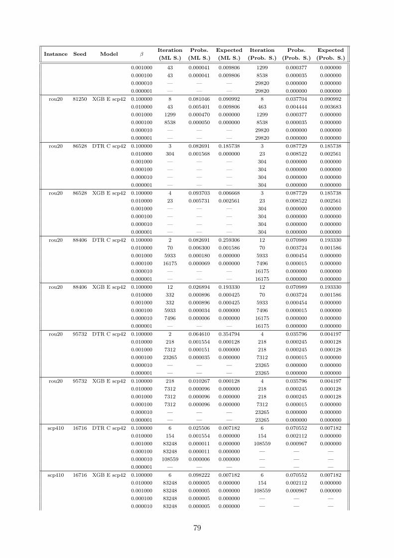
Instance Seed Model β(ML S.)Iteration
(ML S.)Probs.
(ML S.)Expected
(Prob. S.)Iteration
(Prob. S.)Probs.
(Prob. S.)Expected
0.001000 43 0.000041 0.009806 1299 0.000377 0.0000000.000100 43 0.000041 0.009806 8538 0.000035 0.0000000.000010 — — — 29820 0.000000 0.0000000.000001 — — — 29820 0.000000 0.000000
rou20 81250 XGB E scp42 0.100000 8 0.081046 0.090992 8 0.037704 0.0909920.010000 43 0.005401 0.009806 463 0.004444 0.0036830.001000 1299 0.000470 0.000000 1299 0.000377 0.0000000.000100 8538 0.000050 0.000000 8538 0.000035 0.0000000.000010 — — — 29820 0.000000 0.0000000.000001 — — — 29820 0.000000 0.000000
rou20 86528 DTR C scp42 0.100000 3 0.082691 0.185738 3 0.087729 0.1857380.010000 304 0.001568 0.000000 23 0.008522 0.0025610.001000 — — — 304 0.000000 0.0000000.000100 — — — 304 0.000000 0.0000000.000010 — — — 304 0.000000 0.0000000.000001 — — — 304 0.000000 0.000000
rou20 86528 XGB E scp42 0.100000 4 0.093703 0.006668 3 0.087729 0.1857380.010000 23 0.005731 0.002561 23 0.008522 0.0025610.001000 — — — 304 0.000000 0.0000000.000100 — — — 304 0.000000 0.0000000.000010 — — — 304 0.000000 0.0000000.000001 — — — 304 0.000000 0.000000
rou20 88406 DTR C scp42 0.100000 2 0.082691 0.259306 12 0.070989 0.1933300.010000 70 0.006300 0.001586 70 0.003724 0.0015860.001000 5933 0.000180 0.000000 5933 0.000454 0.0000000.000100 16175 0.000069 0.000000 7496 0.000015 0.0000000.000010 — — — 16175 0.000000 0.0000000.000001 — — — 16175 0.000000 0.000000
rou20 88406 XGB E scp42 0.100000 12 0.026894 0.193330 12 0.070989 0.1933300.010000 332 0.000896 0.000425 70 0.003724 0.0015860.001000 332 0.000896 0.000425 5933 0.000454 0.0000000.000100 5933 0.000034 0.000000 7496 0.000015 0.0000000.000010 7496 0.000006 0.000000 16175 0.000000 0.0000000.000001 — — — 16175 0.000000 0.000000
rou20 95732 DTR C scp42 0.100000 2 0.064610 0.354794 4 0.035796 0.0041970.010000 218 0.001554 0.000128 218 0.000245 0.0001280.001000 7312 0.000151 0.000000 218 0.000245 0.0001280.000100 23265 0.000035 0.000000 7312 0.000015 0.0000000.000010 — — — 23265 0.000000 0.0000000.000001 — — — 23265 0.000000 0.000000
rou20 95732 XGB E scp42 0.100000 218 0.010267 0.000128 4 0.035796 0.0041970.010000 7312 0.000096 0.000000 218 0.000245 0.0001280.001000 7312 0.000096 0.000000 218 0.000245 0.0001280.000100 7312 0.000096 0.000000 7312 0.000015 0.0000000.000010 — — — 23265 0.000000 0.0000000.000001 — — — 23265 0.000000 0.000000
scp410 16716 DTR C scp42 0.100000 6 0.025506 0.007182 6 0.070552 0.0071820.010000 154 0.001554 0.000000 154 0.002112 0.0000000.001000 83248 0.000011 0.000000 108559 0.000967 0.0000000.000100 83248 0.000011 0.000000 — — —0.000010 108559 0.000006 0.000000 — — —0.000001 — — — — — —
scp410 16716 XGB E scp42 0.100000 6 0.098222 0.007182 6 0.070552 0.0071820.010000 83248 0.000005 0.000000 154 0.002112 0.0000000.001000 83248 0.000005 0.000000 108559 0.000967 0.0000000.000100 83248 0.000005 0.000000 — — —0.000010 83248 0.000005 0.000000 — — —
79

Instance Seed Model β(ML S.)Iteration
(ML S.)Probs.
(ML S.)Expected
(Prob. S.)Iteration
(Prob. S.)Probs.
(Prob. S.)Expected
0.000001 — — — — — —scp410 20269 DTR C scp42 0.100000 14 0.054826 0.086311 14 0.074967 0.086311
0.010000 357 0.001120 0.000546 357 0.006568 0.0005460.001000 1136 0.000682 0.000000 114094 0.000687 0.0000000.000100 72280 0.000013 0.000000 — — —0.000010 114094 0.000006 0.000000 — — —0.000001 — — — — — —
scp410 20269 XGB E scp42 0.100000 14 0.012236 0.086311 14 0.074967 0.0863110.010000 41 0.005489 0.002825 357 0.006568 0.0005460.001000 357 0.000953 0.000546 114094 0.000687 0.0000000.000100 72280 0.000016 0.000000 — — —0.000010 74618 0.000009 0.000000 — — —0.000001 — — — — — —
scp410 21246 DTR C scp42 0.100000 4 0.038658 0.015743 23 0.034804 0.0110080.010000 109 0.007058 0.004658 222 0.005252 0.0001580.001000 151 0.000398 0.001512 31530 0.000806 0.0000000.000100 10995 0.000085 0.000000 — — —0.000010 100525 0.000007 0.000000 — — —0.000001 344715 0.000001 0.000000 — — —
scp410 21246 XGB E scp42 0.100000 23 0.013640 0.011008 23 0.034804 0.0110080.010000 109 0.008720 0.004658 222 0.005252 0.0001580.001000 3652 0.000433 0.000000 31530 0.000806 0.0000000.000100 10995 0.000014 0.000000 — — —0.000010 100525 0.000004 0.000000 — — —0.000001 344715 0.000001 0.000000 — — —
scp410 39837 DTR C scp42 0.100000 3 0.076681 0.354478 5 0.078386 0.0789120.010000 90 0.009318 0.016491 397 0.009439 0.0022370.001000 8662 0.000122 0.000000 39768 0.000673 0.0000000.000100 21584 0.000035 0.000000 — — —0.000010 146308 0.000005 0.000000 — — —0.000001 535922 0.000001 0.000000 — — —
scp410 39837 XGB E scp42 0.100000 6 0.079251 0.056143 5 0.078386 0.0789120.010000 166 0.005836 0.003136 397 0.009439 0.0022370.001000 8662 0.000060 0.000000 39768 0.000673 0.0000000.000100 8662 0.000060 0.000000 — — —0.000010 146308 0.000005 0.000000 — — —0.000001 535922 0.000001 0.000000 — — —
scp410 40055 DTR C scp42 0.100000 22 0.027368 0.015483 7 0.060554 0.0858060.010000 42 0.002215 0.000676 93 0.009637 0.0004760.001000 704 0.000811 0.000000 39551 0.000576 0.0000000.000100 27060 0.000028 0.000000 — — —0.000010 — — — — — —0.000001 — — — — — —
scp410 40055 XGB E scp42 0.100000 7 0.071467 0.085806 7 0.060554 0.0858060.010000 22 0.003531 0.015483 93 0.009637 0.0004760.001000 704 0.000517 0.000000 39551 0.000576 0.0000000.000100 5912 0.000077 0.000000 — — —0.000010 — — — — — —0.000001 — — — — — —
scp410 4085 DTR C scp42 0.100000 12 0.056393 0.021961 12 0.024688 0.0219610.010000 275 0.002501 0.000438 151 0.009581 0.0073120.001000 3435 0.000727 0.000000 31568 0.001000 0.0000000.000100 31568 0.000028 0.000000 — — —0.000010 102343 0.000007 0.000000 — — —0.000001 — — — — — —
scp410 4085 XGB E scp42 0.100000 5 0.068366 0.365437 12 0.024688 0.0219610.010000 161 0.009851 0.004591 151 0.009581 0.007312
80

Instance Seed Model β(ML S.)Iteration
(ML S.)Probs.
(ML S.)Expected
(Prob. S.)Iteration
(Prob. S.)Probs.
(Prob. S.)Expected
0.001000 3435 0.000403 0.000000 31568 0.001000 0.0000000.000100 31568 0.000024 0.000000 — — —0.000010 102343 0.000005 0.000000 — — —0.000001 — — — — — —
scp410 45150 DTR C scp42 0.100000 3 0.076681 0.852978 4 0.078983 0.3915030.010000 39 0.004795 0.001478 152 0.008536 0.0008800.001000 1820 0.000476 0.000000 89264 0.000995 0.0000000.000100 19525 0.000056 0.000000 — — —0.000010 89264 0.000007 0.000000 — — —0.000001 406554 0.000001 0.000000 — — —
scp410 45150 XGB E scp42 0.100000 10 0.070793 0.271419 4 0.078983 0.3915030.010000 14 -0.003225 0.003747 152 0.008536 0.0008800.001000 14 -0.003225 0.003747 89264 0.000995 0.0000000.000100 14 -0.003225 0.003747 — — —0.000010 14 -0.003225 0.003747 — — —0.000001 14 -0.003225 0.003747 — — —
scp410 5202 DTR C scp42 0.100000 14 0.016479 0.076699 14 0.026542 0.0766990.010000 89 0.006300 0.002591 633 0.004660 0.0000000.001000 178 0.000398 0.001654 146157 0.000880 0.0000000.000100 15816 0.000069 0.000000 — — —0.000010 146157 0.000005 0.000000 — — —0.000001 396744 0.000001 0.000000 — — —
scp410 5202 XGB E scp42 0.100000 6 0.077613 0.334827 14 0.026542 0.0766990.010000 15 0.003926 0.005061 633 0.004660 0.0000000.001000 6581 0.000127 0.000000 146157 0.000880 0.0000000.000100 15816 0.000077 0.000000 — — —0.000010 146157 0.000004 0.000000 — — —0.000001 396744 0.000001 0.000000 — — —
scp410 7057 DTR C scp42 0.100000 4 0.064610 0.373790 38 0.015040 0.0194850.010000 103 0.007058 0.017974 150 0.004888 0.0014730.001000 1403 0.000636 0.000000 87262 0.000497 0.0000000.000100 16031 0.000069 0.000000 — — —0.000010 87262 0.000007 0.000000 — — —0.000001 404572 0.000001 0.000000 — — —
scp410 7057 XGB E scp42 0.100000 4 0.083425 0.373790 38 0.015040 0.0194850.010000 13 -0.002281 0.148697 150 0.004888 0.0014730.001000 13 -0.002281 0.148697 87262 0.000497 0.0000000.000100 13 -0.002281 0.148697 — — —0.000010 13 -0.002281 0.148697 — — —0.000001 13 -0.002281 0.148697 — — —
scp410 93146 DTR C scp42 0.100000 4 0.054172 0.688495 6 0.088469 0.2570910.010000 103 0.007058 0.002461 890 0.005308 0.0000000.001000 890 0.000682 0.000000 54154 0.000577 0.0000000.000100 15470 0.000069 0.000000 — — —0.000010 883090 0.000000 0.000000 — — —0.000001 883090 0.000000 0.000000 — — —
scp410 93146 XGB E scp42 0.100000 4 0.083425 0.688495 6 0.088469 0.2570910.010000 15 0.008408 0.013927 890 0.005308 0.0000000.001000 890 0.000502 0.000000 54154 0.000577 0.0000000.000100 15470 0.000070 0.000000 — — —0.000010 883090 0.000000 0.000000 — — —0.000001 883090 0.000000 0.000000 — — —
scp42 30736 DTR C scp42 0.100000 3 0.082691 0.131915 14 0.078562 0.0599050.010000 112 0.007058 0.008864 776 0.007766 0.0001630.001000 745 0.000811 0.004306 351474 0.000836 0.0000000.000100 12495 0.000085 0.000000 — — —0.000010 351474 0.000001 0.000000 — — —
81

Instance Seed Model β(ML S.)Iteration
(ML S.)Probs.
(ML S.)Expected
(Prob. S.)Iteration
(Prob. S.)Probs.
(Prob. S.)Expected
0.000001 351474 0.000001 0.000000 — — —scp42 30736 XGB E scp42 0.100000 14 0.016621 0.059905 14 0.078562 0.059905
0.010000 112 0.008253 0.008864 776 0.007766 0.0001630.001000 745 0.000462 0.004306 351474 0.000836 0.0000000.000100 12495 0.000025 0.000000 — — —0.000010 85150 0.000007 0.000000 — — —0.000001 351474 0.000001 0.000000 — — —
scp42 40849 DTR C scp42 0.100000 3 0.064610 0.231323 4 0.088859 0.0738860.010000 273 0.002501 0.012760 1767 0.005270 0.0000000.001000 345 0.000154 0.007653 175303 0.000961 0.0000000.000100 87103 0.000007 0.000000 — — —0.000010 87103 0.000007 0.000000 — — —0.000001 618700 0.000001 0.000000 — — —
scp42 40849 XGB E scp42 0.100000 19 0.020575 0.059564 4 0.088859 0.0738860.010000 23 0.005731 0.019547 1767 0.005270 0.0000000.001000 1536 0.000376 0.000008 175303 0.000961 0.0000000.000100 87103 0.000005 0.000000 — — —0.000010 87103 0.000005 0.000000 — — —0.000001 618700 0.000000 0.000000 — — —
scp42 41442 DTR C scp42 0.100000 4 0.064610 0.510226 5 0.055927 0.1018390.010000 105 0.007058 0.012705 517 0.008360 0.0002860.001000 333 0.000154 0.008083 280467 0.000972 0.0000000.000100 103806 0.000007 0.000000 — — —0.000010 103806 0.000007 0.000000 — — —0.000001 582460 0.000001 0.000000 — — —
scp42 41442 XGB E scp42 0.100000 4 0.081438 0.510226 5 0.055927 0.1018390.010000 19 0.002435 0.039499 517 0.008360 0.0002860.001000 103806 0.000006 0.000000 280467 0.000972 0.0000000.000100 103806 0.000006 0.000000 — — —0.000010 103806 0.000006 0.000000 — — —0.000001 582460 0.000001 0.000000 — — —
scp42 43030 DTR C scp42 0.100000 8 0.032036 0.031257 8 0.053163 0.0312570.010000 56 0.004795 0.005784 124 0.004478 0.0001140.001000 777 0.000682 0.000000 764585 0.000637 0.0000000.000100 19003 0.000056 0.000000 — — —0.000010 125357 0.000006 0.000000 — — —0.000001 764585 0.000000 0.000000 — — —
scp42 43030 XGB E scp42 0.100000 8 0.037940 0.031257 8 0.053163 0.0312570.010000 124 0.005576 0.000114 124 0.004478 0.0001140.001000 777 0.000628 0.000000 764585 0.000637 0.0000000.000100 19003 0.000090 0.000000 — — —0.000010 125357 0.000004 0.000000 — — —0.000001 764585 0.000000 0.000000 — — —
scp42 49396 DTR C scp42 0.100000 3 0.038658 0.006636 86 0.017350 0.0056690.010000 86 0.006300 0.005669 702 0.008353 0.0013340.001000 702 0.000811 0.001334 315964 0.000976 0.0000000.000100 17047 0.000064 0.000000 — — —0.000010 112504 0.000006 0.000000 — — —0.000001 362265 0.000001 0.000000 — — —
scp42 49396 XGB E scp42 0.100000 86 0.010974 0.005669 86 0.017350 0.0056690.010000 257 0.003061 0.004161 702 0.008353 0.0013340.001000 702 0.000609 0.001334 315964 0.000976 0.0000000.000100 5716 0.000060 0.000000 — — —0.000010 112504 0.000004 0.000000 — — —0.000001 362265 0.000001 0.000000 — — —
scp42 61403 DTR C scp42 0.100000 13 0.094824 0.028893 4 0.081021 0.1542270.010000 109 0.007058 0.018901 160 0.006276 0.003257
82

Instance Seed Model β(ML S.)Iteration
(ML S.)Probs.
(ML S.)Expected
(Prob. S.)Iteration
(Prob. S.)Probs.
(Prob. S.)Expected
0.001000 2466 0.000822 0.000000 184698 0.000557 0.0000000.000100 9956 0.000078 0.000000 — — —0.000010 184698 0.000002 0.000000 — — —0.000001 — — — — — —
scp42 61403 XGB E scp42 0.100000 7 0.077649 0.115941 4 0.081021 0.1542270.010000 109 0.007695 0.018901 160 0.006276 0.0032570.001000 2466 0.000319 0.000000 184698 0.000557 0.0000000.000100 7427 0.000037 0.000000 — — —0.000010 15283 0.000001 0.000000 — — —0.000001 15283 0.000001 0.000000 — — —
scp42 67807 DTR C scp42 0.100000 223 0.010204 0.009993 223 0.019076 0.0099930.010000 289 0.002501 0.003749 718 0.009745 0.0023150.001000 718 0.000811 0.002315 472054 0.000964 0.0000000.000100 18994 0.000056 0.000000 — — —0.000010 207926 0.000002 0.000000 — — —0.000001 472054 0.000001 0.000000 — — —
scp42 67807 XGB E scp42 0.100000 223 0.019961 0.009993 223 0.019076 0.0099930.010000 289 0.003897 0.003749 718 0.009745 0.0023150.001000 718 0.000597 0.002315 472054 0.000964 0.0000000.000100 40066 0.000024 0.000000 — — —0.000010 207926 0.000002 0.000000 — — —0.000001 472054 0.000001 0.000000 — — —
scp42 72368 DTR C scp42 0.100000 8 0.007752 0.004699 8 0.030394 0.0046990.010000 8 0.007752 0.004699 242 0.007826 0.0001990.001000 242 0.000259 0.000199 20270 0.000625 0.0000000.000100 11010 0.000085 0.000000 — — —0.000010 531973 0.000001 0.000000 — — —0.000001 531973 0.000001 0.000000 — — —
scp42 72368 XGB E scp42 0.100000 4 0.081438 0.209261 8 0.030394 0.0046990.010000 242 0.001690 0.000199 242 0.007826 0.0001990.001000 4661 0.000342 0.000000 20270 0.000625 0.0000000.000100 9468 0.000033 0.000000 — — —0.000010 11010 0.000004 0.000000 — — —0.000001 531973 0.000001 0.000000 — — —
scp42 79312 DTR C scp42 0.100000 6 0.071008 0.053568 8 0.099527 0.0310820.010000 9 0.007752 0.005523 488 0.008913 0.0020680.001000 772 0.000811 0.001306 200670 0.000329 0.0000000.000100 52336 0.000021 0.000000 — — —0.000010 200670 0.000002 0.000000 — — —0.000001 — — — — — —
scp42 79312 XGB E scp42 0.100000 6 0.095635 0.053568 8 0.099527 0.0310820.010000 220 0.001022 0.004416 488 0.008913 0.0020680.001000 488 0.000518 0.002068 200670 0.000329 0.0000000.000100 52336 0.000034 0.000000 — — —0.000010 200670 0.000002 0.000000 — — —0.000001 — — — — — —
scp42 82541 DTR C scp42 0.100000 14 0.043227 0.061019 14 0.064691 0.0610190.010000 96 0.007058 0.026465 573 0.009947 0.0016600.001000 756 0.000811 0.000000 683198 0.000539 0.0000000.000100 95074 0.000007 0.000000 — — —0.000010 95074 0.000007 0.000000 — — —0.000001 584004 0.000001 0.000000 — — —
scp42 82541 XGB E scp42 0.100000 14 0.016621 0.061019 14 0.064691 0.0610190.010000 96 0.008442 0.026465 573 0.009947 0.0016600.001000 756 0.000492 0.000000 683198 0.000539 0.0000000.000100 95074 0.000004 0.000000 — — —0.000010 95074 0.000004 0.000000 — — —
83

Instance Seed Model β(ML S.)Iteration
(ML S.)Probs.
(ML S.)Expected
(Prob. S.)Iteration
(Prob. S.)Probs.
(Prob. S.)Expected
0.000001 584004 0.000000 0.000000 — — —scp49 32335 DTR C scp42 0.100000 6 0.032036 0.004833 43 0.040462 0.004631
0.010000 545 0.006412 0.001220 545 0.007624 0.0012200.001000 1014 0.000682 0.000000 39020 0.000425 0.0000000.000100 10738 0.000085 0.000000 — — —0.000010 — — — — — —0.000001 — — — — — —
scp49 32335 XGB E scp42 0.100000 6 0.098222 0.004833 43 0.040462 0.0046310.010000 545 0.000120 0.001220 545 0.007624 0.0012200.001000 545 0.000120 0.001220 39020 0.000425 0.0000000.000100 10738 0.000012 0.000000 — — —0.000010 — — — — — —0.000001 — — — — — —
scp49 41076 DTR C scp42 0.100000 14 0.034460 0.026884 4 0.089342 0.2897110.010000 138 0.009486 0.012137 166 0.008349 0.0007870.001000 1899 0.000476 0.000000 28115 0.000935 0.0000000.000100 15227 0.000069 0.000000 — — —0.000010 131747 0.000005 0.000000 — — —0.000001 362645 0.000001 0.000000 — — —
scp49 41076 XGB E scp42 0.100000 5 0.070941 0.186815 4 0.089342 0.2897110.010000 14 0.000442 0.026884 166 0.008349 0.0007870.001000 14 0.000442 0.026884 28115 0.000935 0.0000000.000100 15227 0.000072 0.000000 — — —0.000010 131747 0.000005 0.000000 — — —0.000001 225572 0.000001 0.000000 — — —
scp49 41624 DTR C scp42 0.100000 3 0.076681 0.790643 4 0.084348 0.6784820.010000 406 0.002333 0.004554 8 0.009047 0.0264160.001000 18345 0.000060 0.000000 89592 0.000648 0.0000000.000100 18345 0.000060 0.000000 — — —0.000010 89592 0.000007 0.000000 — — —0.000001 812580 0.000000 0.000000 — — —
scp49 41624 XGB E scp42 0.100000 4 0.092714 0.678482 4 0.084348 0.6784820.010000 407 0.003853 0.004396 8 0.009047 0.0264160.001000 18345 0.000097 0.000000 89592 0.000648 0.0000000.000100 18345 0.000097 0.000000 — — —0.000010 89592 0.000006 0.000000 — — —0.000001 812580 0.000000 0.000000 — — —
scp49 43633 DTR C scp42 0.100000 18 0.016479 0.058721 18 0.044419 0.0587210.010000 311 0.002979 0.003776 54 0.009513 0.0128670.001000 920 0.000682 0.000000 5234 0.000652 0.0000000.000100 98435 0.000007 0.000000 — — —0.000010 98435 0.000007 0.000000 — — —0.000001 — — — — — —
scp49 43633 XGB E scp42 0.100000 18 0.020929 0.058721 18 0.044419 0.0587210.010000 159 0.006217 0.007379 54 0.009513 0.0128670.001000 920 0.000458 0.000000 5234 0.000652 0.0000000.000100 98435 0.000005 0.000000 — — —0.000010 98435 0.000005 0.000000 — — —0.000001 — — — — — —
scp49 5178 DTR C scp42 0.100000 22 0.027368 0.018814 22 0.027315 0.0188140.010000 135 0.004777 0.000097 135 0.004868 0.0000970.001000 15611 0.000069 0.000000 128054 0.000524 0.0000000.000100 15611 0.000069 0.000000 — — —0.000010 128054 0.000006 0.000000 — — —0.000001 361123 0.000001 0.000000 — — —
scp49 5178 XGB E scp42 0.100000 7 0.071467 0.206742 22 0.027315 0.0188140.010000 53 0.007113 0.004754 135 0.004868 0.000097
84

Instance Seed Model β(ML S.)Iteration
(ML S.)Probs.
(ML S.)Expected
(Prob. S.)Iteration
(Prob. S.)Probs.
(Prob. S.)Expected
0.001000 15611 0.000018 0.000000 128054 0.000524 0.0000000.000100 15611 0.000018 0.000000 — — —0.000010 128054 0.000004 0.000000 — — —0.000001 361123 0.000001 0.000000 — — —
scp49 54948 DTR C scp42 0.100000 14 0.019625 0.100160 14 0.097574 0.1001600.010000 139 0.009486 0.024690 156 0.008671 0.0038040.001000 1206 0.000636 0.000000 56926 0.000766 0.0000000.000100 17742 0.000064 0.000000 — — —0.000010 514700 0.000001 0.000000 — — —0.000001 514700 0.000001 0.000000 — — —
scp49 54948 XGB E scp42 0.100000 5 0.071295 0.235875 14 0.097574 0.1001600.010000 14 -0.002055 0.100160 156 0.008671 0.0038040.001000 14 -0.002055 0.100160 56926 0.000766 0.0000000.000100 14 -0.002055 0.100160 — — —0.000010 14 -0.002055 0.100160 — — —0.000001 14 -0.002055 0.100160 — — —
scp49 59035 DTR C scp42 0.100000 33 0.016873 0.002036 4 0.079135 0.2953440.010000 917 0.000682 0.000000 33 0.008200 0.0020360.001000 917 0.000682 0.000000 106524 0.000984 0.0000000.000100 10159 0.000078 0.000000 — — —0.000010 106524 0.000007 0.000000 — — —0.000001 — — — — — —
scp49 59035 XGB E scp42 0.100000 8 0.083620 0.072469 4 0.079135 0.2953440.010000 917 0.000571 0.000000 33 0.008200 0.0020360.001000 917 0.000571 0.000000 106524 0.000984 0.0000000.000100 10159 0.000040 0.000000 — — —0.000010 106524 0.000008 0.000000 — — —0.000001 — — — — — —
scp49 75655 DTR C scp42 0.100000 135 0.004777 0.003768 6 0.090484 0.1065850.010000 135 0.004777 0.003768 280 0.009449 0.0011680.001000 868 0.000682 0.000465 21632 0.000860 0.0000000.000100 21632 0.000035 0.000000 — — —0.000010 370314 0.000001 0.000000 — — —0.000001 370314 0.000001 0.000000 — — —
scp49 75655 XGB E scp42 0.100000 6 0.076935 0.106585 6 0.090484 0.1065850.010000 135 0.005086 0.003768 280 0.009449 0.0011680.001000 280 0.000731 0.001168 21632 0.000860 0.0000000.000100 8456 0.000051 0.000000 — — —0.000010 79717 0.000007 0.000000 — — —0.000001 370314 0.000001 0.000000 — — —
scp49 85957 DTR C scp42 0.100000 5 0.079678 0.023098 5 0.052434 0.0230980.010000 100 0.007058 0.009605 542 0.009053 0.0024360.001000 907 0.000682 0.000842 11960 0.000886 0.0000000.000100 11960 0.000085 0.000000 — — —0.000010 86941 0.000007 0.000000 — — —0.000001 391457 0.000001 0.000000 — — —
scp49 85957 XGB E scp42 0.100000 81 0.013197 0.013660 5 0.052434 0.0230980.010000 100 0.008940 0.009605 542 0.009053 0.0024360.001000 542 0.000504 0.002436 11960 0.000886 0.0000000.000100 11960 0.000053 0.000000 — — —0.000010 86941 0.000005 0.000000 — — —0.000001 391457 0.000001 0.000000 — — —
scp49 91691 DTR C scp42 0.100000 14 0.016479 0.003049 14 0.040243 0.0030490.010000 656 0.001233 0.000000 656 0.003012 0.0000000.001000 2501 0.000822 0.000000 34815 0.000699 0.0000000.000100 11477 0.000085 0.000000 — — —0.000010 101132 0.000007 0.000000 — — —
85

Instance Seed Model β(ML S.)Iteration
(ML S.)Probs.
(ML S.)Expected
(Prob. S.)Iteration
(Prob. S.)Probs.
(Prob. S.)Expected
0.000001 — — — — — —scp49 91691 XGB E scp42 0.100000 4 0.092714 0.102385 14 0.040243 0.003049
0.010000 14 -0.002055 0.003049 656 0.003012 0.0000000.001000 14 -0.002055 0.003049 34815 0.000699 0.0000000.000100 14 -0.002055 0.003049 — — —0.000010 14 -0.002055 0.003049 — — —0.000001 14 -0.002055 0.003049 — — —
scp51 16627 DTR C scp42 0.100000 5 0.013186 0.008098 5 0.062135 0.0080980.010000 70 0.006300 0.001957 70 0.005580 0.0019570.001000 4389 0.000266 0.000000 20276 0.000912 0.0000000.000100 10423 0.000078 0.000000 — — —0.000010 112723 0.000006 0.000000 — — —0.000001 505401 0.000001 0.000000 — — —
scp51 16627 XGB E scp42 0.100000 70 0.021450 0.001957 5 0.062135 0.0080980.010000 193 0.001510 0.001010 70 0.005580 0.0019570.001000 4389 0.000395 0.000000 20276 0.000912 0.0000000.000100 8967 0.000027 0.000000 — — —0.000010 112723 0.000005 0.000000 — — —0.000001 505401 0.000001 0.000000 — — —
scp51 23086 DTR C scp42 0.100000 7 0.056393 0.031090 15 0.070165 0.0056210.010000 284 0.000259 0.000568 284 0.007215 0.0005680.001000 284 0.000259 0.000568 55325 0.000932 0.0000000.000100 15441 0.000069 0.000000 — — —0.000010 173128 0.000005 0.000000 — — —0.000001 398061 0.000001 0.000000 — — —
scp51 23086 XGB E scp42 0.100000 7 0.077649 0.031090 15 0.070165 0.0056210.010000 15 0.007503 0.005621 284 0.007215 0.0005680.001000 284 0.000733 0.000568 55325 0.000932 0.0000000.000100 15441 0.000041 0.000000 — — —0.000010 173128 0.000003 0.000000 — — —0.000001 398061 0.000001 0.000000 — — —
scp51 37447 DTR C scp42 0.100000 5 0.079678 0.062219 5 0.059966 0.0622190.010000 120 0.007058 0.004330 597 0.007924 0.0002050.001000 184 0.000398 0.003639 211654 0.000781 0.0000000.000100 13962 0.000069 0.000000 — — —0.000010 211654 0.000002 0.000000 — — —0.000001 733792 0.000000 0.000000 — — —
scp51 37447 XGB E scp42 0.100000 5 0.070941 0.062219 5 0.059966 0.0622190.010000 256 0.005993 0.001352 597 0.007924 0.0002050.001000 4557 0.000556 0.000000 211654 0.000781 0.0000000.000100 9619 0.000036 0.000000 — — —0.000010 211654 0.000001 0.000000 — — —0.000001 211654 0.000001 0.000000 — — —
scp51 41845 DTR C scp42 0.100000 3 0.076681 0.487531 6 0.030997 0.0083190.010000 80 0.006300 0.000666 80 0.005968 0.0006660.001000 1273 0.000636 0.000000 420014 0.000853 0.0000000.000100 18735 0.000060 0.000000 — — —0.000010 420014 0.000001 0.000000 — — —0.000001 420014 0.000001 0.000000 — — —
scp51 41845 XGB E scp42 0.100000 80 0.012515 0.000666 6 0.030997 0.0083190.010000 1273 0.000113 0.000000 80 0.005968 0.0006660.001000 1273 0.000113 0.000000 420014 0.000853 0.0000000.000100 18735 0.000087 0.000000 — — —0.000010 420014 0.000002 0.000000 — — —0.000001 646750 0.000000 0.000000 — — —
scp51 44929 DTR C scp42 0.100000 8 0.013186 0.009771 8 0.036056 0.0097710.010000 509 0.001623 0.004151 2540 0.007827 0.000000
86

Instance Seed Model β(ML S.)Iteration
(ML S.)Probs.
(ML S.)Expected
(Prob. S.)Iteration
(Prob. S.)Probs.
(Prob. S.)Expected
0.001000 800 0.000682 0.002067 68894 0.000721 0.0000000.000100 10176 0.000078 0.000000 — — —0.000010 328284 0.000002 0.000000 — — —0.000001 — — — — — —
scp51 44929 XGB E scp42 0.100000 7 0.077649 0.340866 8 0.036056 0.0097710.010000 180 0.001533 0.008614 2540 0.007827 0.0000000.001000 509 0.000572 0.004151 68894 0.000721 0.0000000.000100 7016 0.000096 0.000000 — — —0.000010 328284 0.000002 0.000000 — — —0.000001 — — — — — —
scp51 51345 DTR C scp42 0.100000 40 0.019047 0.092358 40 0.056778 0.0923580.010000 93 0.007058 0.003001 93 0.006511 0.0030010.001000 700 0.000811 0.001211 34863 0.000765 0.0000000.000100 34863 0.000028 0.000000 — — —0.000010 145593 0.000005 0.000000 — — —0.000001 — — — — — —
scp51 51345 XGB E scp42 0.100000 5 0.072493 0.433968 40 0.056778 0.0923580.010000 40 0.007435 0.092358 93 0.006511 0.0030010.001000 700 0.000482 0.001211 34863 0.000765 0.0000000.000100 4916 0.000064 0.000000 — — —0.000010 145593 0.000001 0.000000 — — —0.000001 145593 0.000001 0.000000 — — —
scp51 72544 DTR C scp42 0.100000 17 0.054826 0.107152 17 0.073228 0.1071520.010000 99 0.007058 0.013281 174 0.008118 0.0053710.001000 386 0.000606 0.004705 37263 0.000943 0.0000000.000100 16786 0.000064 0.000000 — — —0.000010 527879 0.000001 0.000000 — — —0.000001 527879 0.000001 0.000000 — — —
scp51 72544 XGB E scp42 0.100000 17 0.021248 0.107152 17 0.073228 0.1071520.010000 99 0.009671 0.013281 174 0.008118 0.0053710.001000 1227 0.000845 0.000039 37263 0.000943 0.0000000.000100 16786 0.000087 0.000000 — — —0.000010 80823 0.000005 0.000000 — — —0.000001 527879 0.000001 0.000000 — — —
scp51 72556 DTR C scp42 0.100000 3 0.093271 0.060829 70 0.004093 0.0021000.010000 70 0.006300 0.002100 70 0.004093 0.0021000.001000 1549 0.000578 0.000000 13500 0.000706 0.0000000.000100 12213 0.000085 0.000000 — — —0.000010 — — — — — —0.000001 — — — — — —
scp51 72556 XGB E scp42 0.100000 7 0.077643 0.047416 70 0.004093 0.0021000.010000 500 0.000579 0.001080 70 0.004093 0.0021000.001000 500 0.000579 0.001080 13500 0.000706 0.0000000.000100 8619 0.000005 0.000000 — — —0.000010 8619 0.000005 0.000000 — — —0.000001 — — — — — —
scp51 75543 DTR C scp42 0.100000 6 0.071008 0.030678 6 0.069291 0.0306780.010000 535 0.003038 0.001215 535 0.008558 0.0012150.001000 1438 0.000636 0.000000 56629 0.000698 0.0000000.000100 30445 0.000028 0.000000 — — —0.000010 — — — — — —0.000001 — — — — — —
scp51 75543 XGB E scp42 0.100000 6 0.080188 0.030678 6 0.069291 0.0306780.010000 535 0.000553 0.001215 535 0.008558 0.0012150.001000 535 0.000553 0.001215 56629 0.000698 0.0000000.000100 30445 0.000042 0.000000 — — —0.000010 — — — — — —
87

Instance Seed Model β(ML S.)Iteration
(ML S.)Probs.
(ML S.)Expected
(Prob. S.)Iteration
(Prob. S.)Probs.
(Prob. S.)Expected
0.000001 — — — — — —scp51 93582 DTR C scp42 0.100000 34 0.004795 0.003467 5 0.096031 0.312483
0.010000 34 0.004795 0.003467 34 0.006522 0.0034670.001000 992 0.000682 0.000000 507162 0.000685 0.0000000.000100 21114 0.000035 0.000000 — — —0.000010 121918 0.000006 0.000000 — — —0.000001 507162 0.000001 0.000000 — — —
scp51 93582 XGB E scp42 0.100000 5 0.070941 0.312483 5 0.096031 0.3124830.010000 34 0.008257 0.003467 34 0.006522 0.0034670.001000 992 0.000482 0.000000 507162 0.000685 0.0000000.000100 21114 0.000040 0.000000 — — —0.000010 121918 0.000005 0.000000 — — —0.000001 507162 0.000001 0.000000 — — —
scp65 15292 DTR C scp42 0.100000 4 0.038658 0.210955 4 0.082148 0.2109550.010000 40 0.000136 0.023018 565 0.008586 0.0000000.001000 40 0.000136 0.023018 — — —0.000100 13388 0.000085 0.000000 — — —0.000010 339022 0.000002 0.000000 — — —0.000001 — — — — — —
scp65 15292 XGB E scp42 0.100000 4 0.094001 0.210955 4 0.082148 0.2109550.010000 13 -0.003448 0.133240 565 0.008586 0.0000000.001000 13 -0.003448 0.133240 — — —0.000100 13 -0.003448 0.133240 — — —0.000010 13 -0.003448 0.133240 — — —0.000001 13 -0.003448 0.133240 — — —
scp65 17913 DTR C scp42 0.100000 3 0.038658 0.093832 10 0.096232 0.0560650.010000 10 0.000722 0.056065 2043 0.006743 0.0000000.001000 10 0.000722 0.056065 215507 0.000869 0.0000000.000100 33764 0.000028 0.000000 — — —0.000010 134891 0.000005 0.000000 — — —0.000001 — — — — — —
scp65 17913 XGB E scp42 0.100000 10 0.042282 0.056065 10 0.096232 0.0560650.010000 275 0.001705 0.001888 2043 0.006743 0.0000000.001000 605 0.000519 0.000186 215507 0.000869 0.0000000.000100 5846 0.000054 0.000000 — — —0.000010 77634 0.000008 0.000000 — — —0.000001 — — — — — —
scp65 23847 DTR C scp42 0.100000 3 0.054172 0.431519 4 0.095596 0.0383410.010000 44 0.000041 0.025659 361 0.009244 0.0000350.001000 44 0.000041 0.025659 — — —0.000100 44 0.000041 0.025659 — — —0.000010 167458 0.000005 0.000000 — — —0.000001 — — — — — —
scp65 23847 XGB E scp42 0.100000 4 0.081438 0.038341 4 0.095596 0.0383410.010000 274 0.000731 0.006368 361 0.009244 0.0000350.001000 274 0.000731 0.006368 — — —0.000100 13151 0.000011 0.000000 — — —0.000010 167458 0.000003 0.000000 — — —0.000001 — — — — — —
scp65 64414 DTR C scp42 0.100000 3 0.082691 0.062130 7 0.059712 0.0011220.010000 5 0.000722 0.034005 1093 0.008309 0.0000000.001000 5 0.000722 0.034005 — — —0.000100 21437 0.000035 0.000000 — — —0.000010 92779 0.000007 0.000000 — — —0.000001 — — — — — —
scp65 64414 XGB E scp42 0.100000 7 0.070161 0.001122 7 0.059712 0.0011220.010000 1093 0.000080 0.000000 1093 0.008309 0.000000
88

Instance Seed Model β(ML S.)Iteration
(ML S.)Probs.
(ML S.)Expected
(Prob. S.)Iteration
(Prob. S.)Probs.
(Prob. S.)Expected
0.001000 1093 0.000080 0.000000 — — —0.000100 1093 0.000080 0.000000 — — —0.000010 92779 0.000005 0.000000 — — —0.000001 — — — — — —
scp65 70024 DTR C scp42 0.100000 3 0.076681 0.381252 23 0.050117 0.0146170.010000 78 0.006300 0.001207 598 0.009401 0.0000000.001000 1088 0.000682 0.000000 525441 0.000927 0.0000000.000100 24679 0.000028 0.000000 — — —0.000010 100887 0.000007 0.000000 — — —0.000001 525441 0.000001 0.000000 — — —
scp65 70024 XGB E scp42 0.100000 23 0.013640 0.014617 23 0.050117 0.0146170.010000 438 0.000657 0.000667 598 0.009401 0.0000000.001000 438 0.000657 0.000667 525441 0.000927 0.0000000.000100 5849 0.000055 0.000000 — — —0.000010 100887 0.000004 0.000000 — — —0.000001 525441 0.000001 0.000000 — — —
scp65 70336 DTR C scp42 0.100000 3 0.064610 0.590374 4 0.067780 0.0033240.010000 69 0.006300 0.001480 661 0.008724 0.0000000.001000 5459 0.000201 0.000000 — — —0.000100 50898 0.000021 0.000000 — — —0.000010 — — — — — —0.000001 — — — — — —
scp65 70336 XGB E scp42 0.100000 69 0.021450 0.001480 4 0.067780 0.0033240.010000 542 0.000135 0.000922 661 0.008724 0.0000000.001000 542 0.000135 0.000922 — — —0.000100 5520 0.000098 0.000000 — — —0.000010 8718 0.000003 0.000000 — — —0.000001 — — — — — —
scp65 82153 DTR C scp42 0.100000 3 0.064610 0.354989 23 0.044373 0.0546850.010000 37 0.000136 0.008201 560 0.004102 0.0000000.001000 37 0.000136 0.008201 — — —0.000100 53 0.000041 0.001487 — — —0.000010 201111 0.000002 0.000000 — — —0.000001 513075 0.000001 0.000000 — — —
scp65 82153 XGB E scp42 0.100000 8 0.043266 0.347607 23 0.044373 0.0546850.010000 53 0.007867 0.001487 560 0.004102 0.0000000.001000 2996 0.000621 0.000000 — — —0.000100 16607 0.000075 0.000000 — — —0.000010 201111 0.000003 0.000000 — — —0.000001 513075 0.000001 0.000000 — — —
scp65 82443 DTR C scp42 0.100000 3 0.038658 0.051806 71 0.020557 0.0118200.010000 12 0.000722 0.042692 2570 0.006641 0.0000000.001000 12 0.000722 0.042692 436584 0.000943 0.0000000.000100 14424 0.000069 0.000000 — — —0.000010 145858 0.000005 0.000000 — — —0.000001 386342 0.000001 0.000000 — — —
scp65 82443 XGB E scp42 0.100000 12 0.075768 0.042692 71 0.020557 0.0118200.010000 116 0.008644 0.002383 2570 0.006641 0.0000000.001000 2570 0.000306 0.000000 436584 0.000943 0.0000000.000100 8115 0.000030 0.000000 — — —0.000010 145858 0.000005 0.000000 — — —0.000001 386342 0.000001 0.000000 — — —
scp65 88605 DTR C scp42 0.100000 3 0.038658 0.340888 8 0.033213 0.0264360.010000 8 0.000722 0.026436 608 0.008555 0.0003660.001000 8 0.000722 0.026436 — — —0.000100 18683 0.000060 0.000000 — — —0.000010 220666 0.000002 0.000000 — — —
89

Instance Seed Model β(ML S.)Iteration
(ML S.)Probs.
(ML S.)Expected
(Prob. S.)Iteration
(Prob. S.)Probs.
(Prob. S.)Expected
0.000001 — — — — — —scp65 88605 XGB E scp42 0.100000 5 0.067689 0.258162 8 0.033213 0.026436
0.010000 144 0.003877 0.024624 608 0.008555 0.0003660.001000 1715 0.000362 0.000000 — — —0.000100 29777 0.000031 0.000000 — — —0.000010 84888 0.000006 0.000000 — — —0.000001 — — — — — —
scp65 95465 DTR C scp42 0.100000 3 0.082691 0.652128 6 0.027055 0.2296390.010000 17 0.003334 0.170425 419 0.006041 0.0000000.001000 32 0.000136 0.007504 — — —0.000100 10671 0.000085 0.000000 — — —0.000010 — — — — — —0.000001 — — — — — —
scp65 95465 XGB E scp42 0.100000 17 0.020575 0.170425 6 0.027055 0.2296390.010000 22 0.003560 0.143729 419 0.006041 0.0000000.001000 10671 0.000043 0.000000 — — —0.000100 10671 0.000043 0.000000 — — —0.000010 — — — — — —0.000001 — — — — — —
scpa4 20206 DTR C scp42 0.100000 3 0.093271 0.096107 37 0.049579 0.0252700.010000 5945 0.000180 0.000000 5945 0.002491 0.0000000.001000 5945 0.000180 0.000000 83608 0.000978 0.0000000.000100 13858 0.000069 0.000000 — — —0.000010 232382 0.000002 0.000000 — — —0.000001 359300 0.000001 0.000000 — — —
scpa4 20206 XGB E scp42 0.100000 37 0.024186 0.025270 37 0.049579 0.0252700.010000 5945 0.000142 0.000000 5945 0.002491 0.0000000.001000 5945 0.000142 0.000000 83608 0.000978 0.0000000.000100 13858 0.000041 0.000000 — — —0.000010 232382 0.000002 0.000000 — — —0.000001 359300 0.000001 0.000000 — — —
scpa4 31872 DTR C scp42 0.100000 3 0.082691 0.046685 21 0.066924 0.0340570.010000 78 0.006300 0.000621 78 0.006439 0.0006210.001000 952 0.000682 0.000000 19958 0.000769 0.0000000.000100 9803 0.000078 0.000000 — — —0.000010 255706 0.000002 0.000000 — — —0.000001 436872 0.000001 0.000000 — — —
scpa4 31872 XGB E scp42 0.100000 21 0.023196 0.034057 21 0.066924 0.0340570.010000 574 0.000032 0.000000 78 0.006439 0.0006210.001000 574 0.000032 0.000000 19958 0.000769 0.0000000.000100 574 0.000032 0.000000 — — —0.000010 255706 0.000002 0.000000 — — —0.000001 436872 0.000001 0.000000 — — —
scpa4 40563 DTR C scp42 0.100000 12 0.043126 0.033515 12 0.041526 0.0335150.010000 34 0.004795 0.002866 98 0.007641 0.0001630.001000 818 0.000682 0.000000 3921 0.000947 0.0000000.000100 100770 0.000007 0.000000 — — —0.000010 100770 0.000007 0.000000 — — —0.000001 832896 0.000000 0.000000 — — —
scpa4 40563 XGB E scp42 0.100000 12 0.075979 0.033515 12 0.041526 0.0335150.010000 98 0.007710 0.000163 98 0.007641 0.0001630.001000 818 0.000597 0.000000 3921 0.000947 0.0000000.000100 100770 0.000009 0.000000 — — —0.000010 100770 0.000009 0.000000 — — —0.000001 832896 0.000000 0.000000 — — —
scpa4 4516 DTR C scp42 0.100000 4 0.082691 0.072601 4 0.078863 0.0726010.010000 73 0.006300 0.000743 73 0.006894 0.000743
90

Instance Seed Model β(ML S.)Iteration
(ML S.)Probs.
(ML S.)Expected
(Prob. S.)Iteration
(Prob. S.)Probs.
(Prob. S.)Expected
0.001000 2202 0.000348 0.000000 93242 0.000452 0.0000000.000100 15464 0.000069 0.000000 — — —0.000010 93242 0.000007 0.000000 — — —0.000001 — — — — — —
scpa4 4516 XGB E scp42 0.100000 4 0.092714 0.072601 4 0.078863 0.0726010.010000 26 0.007984 0.065036 73 0.006894 0.0007430.001000 2202 0.000360 0.000000 93242 0.000452 0.0000000.000100 15464 0.000041 0.000000 — — —0.000010 93242 0.000005 0.000000 — — —0.000001 — — — — — —
scpa4 46197 DTR C scp42 0.100000 8 0.064610 0.090013 5 0.091107 0.1437870.010000 17 0.003334 0.001155 572 0.004202 0.0000000.001000 2440 0.000822 0.000000 164561 0.000617 0.0000000.000100 22569 0.000035 0.000000 — — —0.000010 132671 0.000005 0.000000 — — —0.000001 512103 0.000001 0.000000 — — —
scpa4 46197 XGB E scp42 0.100000 5 0.071295 0.143787 5 0.091107 0.1437870.010000 17 0.001086 0.001155 572 0.004202 0.0000000.001000 2440 0.000342 0.000000 164561 0.000617 0.0000000.000100 22569 0.000048 0.000000 — — —0.000010 132671 0.000003 0.000000 — — —0.000001 512103 0.000001 0.000000 — — —
scpa4 62924 DTR C scp42 0.100000 23 0.027368 0.063681 23 0.021731 0.0636810.010000 33 0.002215 0.000292 33 0.001489 0.0002920.001000 10644 0.000085 0.000000 10644 0.000560 0.0000000.000100 10644 0.000085 0.000000 — — —0.000010 610230 0.000001 0.000000 — — —0.000001 610230 0.000001 0.000000 — — —
scpa4 62924 XGB E scp42 0.100000 23 0.012083 0.063681 23 0.021731 0.0636810.010000 435 0.000635 0.000000 33 0.001489 0.0002920.001000 435 0.000635 0.000000 10644 0.000560 0.0000000.000100 10644 0.000069 0.000000 — — —0.000010 610230 0.000001 0.000000 — — —0.000001 610230 0.000001 0.000000 — — —
scpa4 72427 DTR C scp42 0.100000 3 0.064610 0.347092 26 0.018633 0.0313320.010000 559 0.006412 0.006223 889 0.007938 0.0016650.001000 889 0.000682 0.001665 17980 0.000870 0.0000000.000100 17980 0.000060 0.000000 — — —0.000010 200253 0.000002 0.000000 — — —0.000001 612099 0.000001 0.000000 — — —
scpa4 72427 XGB E scp42 0.100000 15 0.015256 0.218992 26 0.018633 0.0313320.010000 33 0.007128 0.022383 889 0.007938 0.0016650.001000 889 0.000490 0.001665 17980 0.000870 0.0000000.000100 8218 0.000030 0.000000 — — —0.000010 200253 0.000001 0.000000 — — —0.000001 200253 0.000001 0.000000 — — —
scpa4 79587 DTR C scp42 0.100000 14 0.054826 0.190415 33 0.097117 0.0769630.010000 109 0.007058 0.013011 315 0.008530 0.0021410.001000 67483 0.000019 0.000000 207401 0.000982 0.0000000.000100 67483 0.000019 0.000000 — — —0.000010 105944 0.000007 0.000000 — — —0.000001 890802 0.000000 0.000000 — — —
scpa4 79587 XGB E scp42 0.100000 14 0.016036 0.190415 33 0.097117 0.0769630.010000 22 0.000537 0.105076 315 0.008530 0.0021410.001000 22 0.000537 0.105076 207401 0.000982 0.0000000.000100 67483 0.000015 0.000000 — — —0.000010 105944 0.000006 0.000000 — — —
91

Instance Seed Model β(ML S.)Iteration
(ML S.)Probs.
(ML S.)Expected
(Prob. S.)Iteration
(Prob. S.)Probs.
(Prob. S.)Expected
0.000001 890802 0.000000 0.000000 — — —scpa4 82496 DTR C scp42 0.100000 4 0.038658 0.029849 4 0.098892 0.029849
0.010000 311 0.001568 0.002788 311 0.009736 0.0027880.001000 3490 0.000727 0.000000 50560 0.000496 0.0000000.000100 30819 0.000028 0.000000 — — —0.000010 366694 0.000001 0.000000 — — —0.000001 366694 0.000001 0.000000 — — —
scpa4 82496 XGB E scp42 0.100000 4 0.093703 0.029849 4 0.098892 0.0298490.010000 311 0.001509 0.002788 311 0.009736 0.0027880.001000 406 0.000748 0.001339 50560 0.000496 0.0000000.000100 30819 0.000042 0.000000 — — —0.000010 366694 0.000001 0.000000 — — —0.000001 366694 0.000001 0.000000 — — —
scpa4 84917 DTR C scp42 0.100000 8 0.013186 0.008544 8 0.009093 0.0085440.010000 495 0.001623 0.000074 8 0.009093 0.0085440.001000 802 0.000682 0.000000 9374 0.000750 0.0000000.000100 384880 0.000001 0.000000 — — —0.000010 384880 0.000001 0.000000 — — —0.000001 384880 0.000001 0.000000 — — —
scpa4 84917 XGB E scp42 0.100000 4 0.083425 0.643664 8 0.009093 0.0085440.010000 495 0.000541 0.000074 8 0.009093 0.0085440.001000 495 0.000541 0.000074 9374 0.000750 0.0000000.000100 9374 0.000000 0.000000 — — —0.000010 9374 0.000000 0.000000 — — —0.000001 9374 0.000000 0.000000 — — —
scpb3 13133 DTR C scp42 0.100000 3 0.038658 0.588154 5 0.058029 0.0388920.010000 5 0.000722 0.038892 9662 0.009676 0.0000000.001000 5 0.000722 0.038892 — — —0.000100 10622 0.000085 0.000000 — — —0.000010 704667 0.000000 0.000000 — — —0.000001 704667 0.000000 0.000000 — — —
scpb3 13133 XGB E scp42 0.100000 10 0.071729 0.006609 5 0.058029 0.0388920.010000 314 0.002937 0.005896 9662 0.009676 0.0000000.001000 527 0.000496 0.004161 — — —0.000100 7182 0.000092 0.000000 — — —0.000010 704667 0.000000 0.000000 — — —0.000001 704667 0.000000 0.000000 — — —
scpb3 34257 DTR C scp42 0.100000 3 0.038658 0.400431 5 0.084194 0.1956100.010000 5 0.000722 0.195610 8013 0.009323 0.0000000.001000 5 0.000722 0.195610 — — —0.000100 20118 0.000045 0.000000 — — —0.000010 95214 0.000007 0.000000 — — —0.000001 806015 0.000000 0.000000 — — —
scpb3 34257 XGB E scp42 0.100000 12 0.077073 0.073876 5 0.084194 0.1956100.010000 457 0.000517 0.000000 8013 0.009323 0.0000000.001000 457 0.000517 0.000000 — — —0.000100 8013 0.000025 0.000000 — — —0.000010 95214 0.000010 0.000000 — — —0.000001 806015 0.000000 0.000000 — — —
scpb3 4964 DTR C scp42 0.100000 3 0.038658 0.387150 6 0.032844 0.0193170.010000 6 0.000722 0.019317 7318 0.005992 0.0000000.001000 6 0.000722 0.019317 — — —0.000100 57996 0.000021 0.000000 — — —0.000010 98429 0.000007 0.000000 — — —0.000001 — — — — — —
scpb3 4964 XGB E scp42 0.100000 6 0.098222 0.019317 6 0.032844 0.0193170.010000 1173 0.000059 0.000000 7318 0.005992 0.000000
92

Instance Seed Model β(ML S.)Iteration
(ML S.)Probs.
(ML S.)Expected
(Prob. S.)Iteration
(Prob. S.)Probs.
(Prob. S.)Expected
0.001000 1173 0.000059 0.000000 — — —0.000100 1173 0.000059 0.000000 — — —0.000010 70917 0.000006 0.000000 — — —0.000001 — — — — — —
scpb3 66361 DTR C scp42 0.100000 3 0.038658 0.124344 57 0.092362 0.0612390.010000 6 0.000722 0.093677 2744 0.007861 0.0000000.001000 6 0.000722 0.093677 — — —0.000100 54847 0.000021 0.000000 — — —0.000010 206217 0.000002 0.000000 — — —0.000001 342279 0.000001 0.000000 — — —
scpb3 66361 XGB E scp42 0.100000 6 0.079251 0.093677 57 0.092362 0.0612390.010000 75 0.006391 0.003696 2744 0.007861 0.0000000.001000 1123 0.000459 0.000000 — — —0.000100 54847 0.000015 0.000000 — — —0.000010 206217 0.000003 0.000000 — — —0.000001 342279 0.000001 0.000000 — — —
scpb3 71918 DTR C scp42 0.100000 3 0.038658 0.303578 9 0.053349 0.0759530.010000 5 0.000722 0.209618 739 0.007752 0.0000000.001000 5 0.000722 0.209618 — — —0.000100 23759 0.000035 0.000000 — — —0.000010 86646 0.000007 0.000000 — — —0.000001 493464 0.000001 0.000000 — — —
scpb3 71918 XGB E scp42 0.100000 5 0.071295 0.209618 9 0.053349 0.0759530.010000 185 0.002034 0.001615 739 0.007752 0.0000000.001000 739 0.000543 0.000000 — — —0.000100 23759 0.000044 0.000000 — — —0.000010 125643 0.000004 0.000000 — — —0.000001 493464 0.000001 0.000000 — — —
scpb3 8320 DTR C scp42 0.100000 3 0.038658 0.417638 8 0.057808 0.1842160.010000 8 0.000722 0.184216 3866 0.008025 0.0000000.001000 8 0.000722 0.184216 — — —0.000100 9993 0.000078 0.000000 — — —0.000010 510116 0.000001 0.000000 — — —0.000001 510116 0.000001 0.000000 — — —
scpb3 8320 XGB E scp42 0.100000 8 0.082684 0.184216 8 0.057808 0.1842160.010000 3866 0.000480 0.000000 3866 0.008025 0.0000000.001000 3866 0.000480 0.000000 — — —0.000100 9993 0.000033 0.000000 — — —0.000010 510116 0.000001 0.000000 — — —0.000001 510116 0.000001 0.000000 — — —
scpb3 8536 DTR C scp42 0.100000 3 0.038658 0.471312 4 0.082857 0.3350980.010000 5 0.000722 0.230255 136 0.006803 0.0000000.001000 5 0.000722 0.230255 — — —0.000100 19956 0.000045 0.000000 — — —0.000010 388100 0.000001 0.000000 — — —0.000001 388100 0.000001 0.000000 — — —
scpb3 8536 XGB E scp42 0.100000 4 0.092714 0.335098 4 0.082857 0.3350980.010000 17 0.001086 0.010739 136 0.006803 0.0000000.001000 8007 0.000028 0.000000 — — —0.000100 8007 0.000028 0.000000 — — —0.000010 388100 0.000001 0.000000 — — —0.000001 388100 0.000001 0.000000 — — —
scpb3 94506 DTR C scp42 0.100000 3 0.038658 0.124261 42 0.085618 0.0813890.010000 42 0.000041 0.081389 1956 0.006703 0.0000000.001000 42 0.000041 0.081389 — — —0.000100 42 0.000041 0.081389 — — —0.000010 252739 0.000002 0.000000 — — —
93

Instance Seed Model β(ML S.)Iteration
(ML S.)Probs.
(ML S.)Expected
(Prob. S.)Iteration
(Prob. S.)Probs.
(Prob. S.)Expected
0.000001 — — — — — —scpb3 94506 XGB E scp42 0.100000 42 0.023654 0.081389 42 0.085618 0.081389
0.010000 342 0.001576 0.001703 1956 0.006703 0.0000000.001000 627 0.000522 0.000430 — — —0.000100 252739 0.000002 0.000000 — — —0.000010 252739 0.000002 0.000000 — — —0.000001 — — — — — —
scpb3 97529 DTR C scp42 0.100000 3 0.038658 0.241430 18 0.096002 0.0876040.010000 5 0.000722 0.202311 1708 0.006748 0.0000000.001000 5 0.000722 0.202311 — — —0.000100 45 0.000041 0.014720 — — —0.000010 133704 0.000005 0.000000 — — —0.000001 955240 0.000000 0.000000 — — —
scpb3 97529 XGB E scp42 0.100000 5 0.071295 0.202311 18 0.096002 0.0876040.010000 18 0.002435 0.087604 1708 0.006748 0.0000000.001000 1050 0.000881 0.000000 — — —0.000100 67983 0.000014 0.000000 — — —0.000010 133704 0.000005 0.000000 — — —0.000001 955240 0.000000 0.000000 — — —
scpb3 9925 DTR C scp42 0.100000 3 0.038658 0.674091 5 0.074105 0.2296590.010000 5 0.000722 0.229659 870 0.008640 0.0000000.001000 5 0.000722 0.229659 — — —0.000100 56 0.000041 0.002009 — — —0.000010 107579 0.000007 0.000000 — — —0.000001 — — — — — —
scpb3 9925 XGB E scp42 0.100000 4 0.093703 0.580180 5 0.074105 0.2296590.010000 13 0.000437 0.117951 870 0.008640 0.0000000.001000 13 0.000437 0.117951 — — —0.000100 47961 0.000022 0.000000 — — —0.000010 107579 0.000006 0.000000 — — —0.000001 — — — — — —
scpc1 1049 DTR C scp42 0.100000 12 0.013186 0.218074 4 0.092296 0.2915380.010000 306 0.001568 0.004460 592 0.005362 0.0010070.001000 1278 0.000636 0.000000 26133 0.000856 0.0000000.000100 11247 0.000085 0.000000 — — —0.000010 132059 0.000005 0.000000 — — —0.000001 — — — — — —
scpc1 1049 XGB E scp42 0.100000 4 0.092657 0.291538 4 0.092296 0.2915380.010000 16 0.001099 0.046587 592 0.005362 0.0010070.001000 2017 0.000636 0.000000 26133 0.000856 0.0000000.000100 9710 0.000039 0.000000 — — —0.000010 132059 0.000001 0.000000 — — —0.000001 132059 0.000001 0.000000 — — —
scpc1 12401 DTR C scp42 0.100000 11 0.013186 0.020792 11 0.040829 0.0207920.010000 17 0.003334 0.018825 309 0.009211 0.0032840.001000 4108 0.000283 0.000000 8552 0.000839 0.0000000.000100 23471 0.000035 0.000000 — — —0.000010 — — — — — —0.000001 — — — — — —
scpc1 12401 XGB E scp42 0.100000 4 0.092657 0.208861 11 0.040829 0.0207920.010000 17 0.001101 0.018825 309 0.009211 0.0032840.001000 4108 0.000410 0.000000 8552 0.000839 0.0000000.000100 7424 0.000079 0.000000 — — —0.000010 — — — — — —0.000001 — — — — — —
scpc1 29296 DTR C scp42 0.100000 5 0.025506 0.028339 5 0.067407 0.0283390.010000 459 0.002238 0.002471 459 0.006107 0.002471
94

Instance Seed Model β(ML S.)Iteration
(ML S.)Probs.
(ML S.)Expected
(Prob. S.)Iteration
(Prob. S.)Probs.
(Prob. S.)Expected
0.001000 1463 0.000636 0.000000 1463 0.000874 0.0000000.000100 116453 0.000006 0.000000 — — —0.000010 116453 0.000006 0.000000 — — —0.000001 — — — — — —
scpc1 29296 XGB E scp42 0.100000 14 0.016695 0.020499 5 0.067407 0.0283390.010000 459 0.000517 0.002471 459 0.006107 0.0024710.001000 459 0.000517 0.002471 1463 0.000874 0.0000000.000100 116453 0.000006 0.000000 — — —0.000010 116453 0.000006 0.000000 — — —0.000001 — — — — — —
scpc1 3065 DTR C scp42 0.100000 4 0.038658 0.017972 38 0.025318 0.0115990.010000 99 0.007058 0.006657 99 0.009924 0.0066570.001000 228 0.000398 0.004878 10287 0.000752 0.0000000.000100 10287 0.000078 0.000000 — — —0.000010 205869 0.000002 0.000000 — — —0.000001 396526 0.000001 0.000000 — — —
scpc1 3065 XGB E scp42 0.100000 38 0.024644 0.011599 38 0.025318 0.0115990.010000 99 0.008240 0.006657 99 0.009924 0.0066570.001000 302 0.000912 0.004267 10287 0.000752 0.0000000.000100 10287 0.000051 0.000000 — — —0.000010 205869 0.000002 0.000000 — — —0.000001 396526 0.000001 0.000000 — — —
scpc1 35343 DTR C scp42 0.100000 15 0.043227 0.081675 15 0.052878 0.0816750.010000 406 0.002333 0.005498 21 0.009787 0.0062720.001000 778 0.000682 0.000000 6065 0.000501 0.0000000.000100 405613 0.000001 0.000000 — — —0.000010 405613 0.000001 0.000000 — — —0.000001 405613 0.000001 0.000000 — — —
scpc1 35343 XGB E scp42 0.100000 15 0.009710 0.081675 15 0.052878 0.0816750.010000 15 0.009710 0.081675 21 0.009787 0.0062720.001000 778 0.000604 0.000000 6065 0.000501 0.0000000.000100 6065 0.000024 0.000000 — — —0.000010 405613 0.000001 0.000000 — — —0.000001 405613 0.000001 0.000000 — — —
scpc1 40226 DTR C scp42 0.100000 14 0.043227 0.062633 14 0.013823 0.0626330.010000 17 0.003334 0.014871 17 0.009979 0.0148710.001000 3087 0.000385 0.000000 67668 0.000662 0.0000000.000100 22002 0.000035 0.000000 — — —0.000010 86545 0.000007 0.000000 — — —0.000001 — — — — — —
scpc1 40226 XGB E scp42 0.100000 14 0.017350 0.062633 14 0.013823 0.0626330.010000 3087 0.000569 0.000000 17 0.009979 0.0148710.001000 3087 0.000569 0.000000 67668 0.000662 0.0000000.000100 5605 0.000078 0.000000 — — —0.000010 86545 0.000004 0.000000 — — —0.000001 — — — — — —
scpc1 54123 DTR C scp42 0.100000 3 0.064610 0.102706 44 0.001232 0.0001460.010000 44 0.002215 0.000146 44 0.001232 0.0001460.001000 4626 0.000266 0.000000 59261 0.000300 0.0000000.000100 21389 0.000035 0.000000 — — —0.000010 776521 0.000000 0.000000 — — —0.000001 776521 0.000000 0.000000 — — —
scpc1 54123 XGB E scp42 0.100000 44 0.026683 0.000146 44 0.001232 0.0001460.010000 4626 0.000328 0.000000 44 0.001232 0.0001460.001000 4626 0.000328 0.000000 59261 0.000300 0.0000000.000100 21389 0.000046 0.000000 — — —0.000010 776521 0.000000 0.000000 — — —
95

Instance Seed Model β(ML S.)Iteration
(ML S.)Probs.
(ML S.)Expected
(Prob. S.)Iteration
(Prob. S.)Probs.
(Prob. S.)Expected
0.000001 776521 0.000000 0.000000 — — —scpc1 64402 DTR C scp42 0.100000 3 0.082691 0.025613 87 0.037151 0.015709
0.010000 99 0.007058 0.000879 1421 0.001172 0.0000000.001000 1421 0.000636 0.000000 48892 0.000727 0.0000000.000100 25878 0.000028 0.000000 — — —0.000010 — — — — — —0.000001 — — — — — —
scpc1 64402 XGB E scp42 0.100000 87 0.020647 0.015709 87 0.037151 0.0157090.010000 1421 0.000120 0.000000 1421 0.001172 0.0000000.001000 1421 0.000120 0.000000 48892 0.000727 0.0000000.000100 25878 0.000040 0.000000 — — —0.000010 81535 0.000005 0.000000 — — —0.000001 — — — — — —
scpc1 75033 DTR C scp42 0.100000 3 0.054172 0.012717 77 0.033678 0.0119760.010000 102 0.007058 0.006179 454 0.008675 0.0031760.001000 364 0.000606 0.005519 18064 0.000828 0.0000000.000100 15288 0.000069 0.000000 — — —0.000010 320173 0.000002 0.000000 — — —0.000001 600280 0.000001 0.000000 — — —
scpc1 75033 XGB E scp42 0.100000 77 0.019762 0.011976 77 0.033678 0.0119760.010000 364 0.002731 0.005519 454 0.008675 0.0031760.001000 454 0.000517 0.003176 18064 0.000828 0.0000000.000100 6946 0.000050 0.000000 — — —0.000010 74357 0.000010 0.000000 — — —0.000001 600280 0.000001 0.000000 — — —
scpc1 97250 DTR C scp42 0.100000 10 0.056393 0.141088 10 0.035548 0.1410880.010000 84 0.006300 0.005621 768 0.003874 0.0000000.001000 768 0.000811 0.000000 6870 0.000778 0.0000000.000100 47354 0.000025 0.000000 — — —0.000010 86546 0.000007 0.000000 — — —0.000001 573208 0.000001 0.000000 — — —
scpc1 97250 XGB E scp42 0.100000 10 0.070793 0.141088 10 0.035548 0.1410880.010000 97 0.008234 0.005493 768 0.003874 0.0000000.001000 768 0.000443 0.000000 6870 0.000778 0.0000000.000100 47354 0.000020 0.000000 — — —0.000010 86546 0.000005 0.000000 — — —0.000001 573208 0.000001 0.000000 — — —
scpd1 12316 DTR C scp42 0.100000 3 0.038658 0.059258 12 0.051945 0.0165030.010000 12 0.000722 0.016503 4071 0.008755 0.0000000.001000 12 0.000722 0.016503 — — —0.000100 25163 0.000028 0.000000 — — —0.000010 93186 0.000007 0.000000 — — —0.000001 — — — — — —
scpd1 12316 XGB E scp42 0.100000 12 0.032007 0.016503 12 0.051945 0.0165030.010000 153 0.003473 0.012179 4071 0.008755 0.0000000.001000 406 0.000670 0.004247 — — —0.000100 9779 0.000054 0.000000 — — —0.000010 93186 0.000006 0.000000 — — —0.000001 — — — — — —
scpd1 13826 DTR C scp42 0.100000 3 0.038658 0.260261 12 0.082157 0.1024770.010000 12 0.000722 0.102477 3580 0.005288 0.0000000.001000 12 0.000722 0.102477 — — —0.000100 18675 0.000060 0.000000 — — —0.000010 149685 0.000005 0.000000 — — —0.000001 533386 0.000001 0.000000 — — —
scpd1 13826 XGB E scp42 0.100000 12 0.082026 0.102477 12 0.082157 0.1024770.010000 130 0.005303 0.001321 3580 0.005288 0.000000
96

Instance Seed Model β(ML S.)Iteration
(ML S.)Probs.
(ML S.)Expected
(Prob. S.)Iteration
(Prob. S.)Probs.
(Prob. S.)Expected
0.001000 561 0.000572 0.000272 — — —0.000100 149685 0.000003 0.000000 — — —0.000010 149685 0.000003 0.000000 — — —0.000001 533386 0.000001 0.000000 — — —
scpd1 23931 DTR C scp42 0.100000 3 0.038658 0.065585 27 0.092350 0.0215260.010000 54 0.000041 0.008832 2207 0.006289 0.0000000.001000 54 0.000041 0.008832 — — —0.000100 54 0.000041 0.008832 — — —0.000010 97034 0.000007 0.000000 — — —0.000001 — — — — — —
scpd1 23931 XGB E scp42 0.100000 25 0.023196 0.048665 27 0.092350 0.0215260.010000 213 0.001067 0.006583 2207 0.006289 0.0000000.001000 253 0.000623 0.002380 — — —0.000100 26199 0.000042 0.000000 — — —0.000010 97034 0.000004 0.000000 — — —0.000001 — — — — — —
scpd1 26284 DTR C scp42 0.100000 3 0.038658 0.369192 8 0.055505 0.0167290.010000 8 0.000722 0.016729 1768 0.007893 0.0000000.001000 8 0.000722 0.016729 — — —0.000100 72113 0.000013 0.000000 — — —0.000010 153614 0.000005 0.000000 — — —0.000001 524113 0.000001 0.000000 — — —
scpd1 26284 XGB E scp42 0.100000 8 0.086416 0.016729 8 0.055505 0.0167290.010000 138 0.005441 0.003015 1768 0.007893 0.0000000.001000 402 0.000670 0.000000 — — —0.000100 72113 0.000007 0.000000 — — —0.000010 72113 0.000007 0.000000 — — —0.000001 524113 0.000001 0.000000 — — —
scpd1 44691 DTR C scp42 0.100000 3 0.038658 0.569987 7 0.090705 0.5263130.010000 7 0.000722 0.526313 9796 0.007974 0.0000000.001000 7 0.000722 0.526313 — — —0.000100 54 0.000041 0.035017 — — —0.000010 167535 0.000005 0.000000 — — —0.000001 877177 0.000000 0.000000 — — —
scpd1 44691 XGB E scp42 0.100000 7 0.076837 0.526313 7 0.090705 0.5263130.010000 20 0.002018 0.165522 9796 0.007974 0.0000000.001000 1480 0.000383 0.000000 — — —0.000100 9228 0.000036 0.000000 — — —0.000010 78720 0.000005 0.000000 — — —0.000001 167535 0.000001 0.000000 — — —
scpd1 45107 DTR C scp42 0.100000 3 0.038658 0.687723 4 0.082317 0.1021460.010000 7 0.000722 0.090679 10462 0.005442 0.0000000.001000 7 0.000722 0.090679 — — —0.000100 55 0.000041 0.032128 — — —0.000010 122881 0.000006 0.000000 — — —0.000001 714485 0.000000 0.000000 — — —
scpd1 45107 XGB E scp42 0.100000 7 0.076837 0.090679 4 0.082317 0.1021460.010000 37 0.008146 0.035119 10462 0.005442 0.0000000.001000 4738 0.000642 0.000000 — — —0.000100 10462 0.000086 0.000000 — — —0.000010 122881 0.000005 0.000000 — — —0.000001 714485 0.000000 0.000000 — — —
scpd1 45796 DTR C scp42 0.100000 3 0.038658 0.143832 22 0.098519 0.1237510.010000 32 0.000136 0.072935 1258 0.006181 0.0000000.001000 32 0.000136 0.072935 — — —0.000100 41 0.000041 0.070585 — — —0.000010 132801 0.000005 0.000000 — — —
97

Instance Seed Model β(ML S.)Iteration
(ML S.)Probs.
(ML S.)Expected
(Prob. S.)Iteration
(Prob. S.)Probs.
(Prob. S.)Expected
0.000001 779093 0.000000 0.000000 — — —scpd1 45796 XGB E scp42 0.100000 22 0.024395 0.123751 22 0.098519 0.123751
0.010000 51 0.003920 0.005479 1258 0.006181 0.0000000.001000 1258 0.000559 0.000000 — — —0.000100 15724 0.000045 0.000000 — — —0.000010 132801 0.000003 0.000000 — — —0.000001 779093 0.000000 0.000000 — — —
scpd1 70795 DTR C scp42 0.100000 3 0.038658 0.242844 7 0.057856 0.0884430.010000 7 0.000722 0.088443 6363 0.009042 0.0000000.001000 7 0.000722 0.088443 — — —0.000100 46 0.000041 0.008465 — — —0.000010 — — — — — —0.000001 — — — — — —
scpd1 70795 XGB E scp42 0.100000 7 0.088498 0.088443 7 0.057856 0.0884430.010000 123 0.007457 0.004657 6363 0.009042 0.0000000.001000 681 0.000513 0.003102 — — —0.000100 47371 0.000018 0.000000 — — —0.000010 — — — — — —0.000001 — — — — — —
scpd1 73667 DTR C scp42 0.100000 3 0.038658 0.011801 42 0.036840 0.0033380.010000 42 0.000041 0.003338 2566 0.006134 0.0000000.001000 42 0.000041 0.003338 — — —0.000100 42 0.000041 0.003338 — — —0.000010 101661 0.000007 0.000000 — — —0.000001 360467 0.000001 0.000000 — — —
scpd1 73667 XGB E scp42 0.100000 42 0.022094 0.003338 42 0.036840 0.0033380.010000 1085 0.000087 0.000000 2566 0.006134 0.0000000.001000 1085 0.000087 0.000000 — — —0.000100 1085 0.000087 0.000000 — — —0.000010 149893 0.000003 0.000000 — — —0.000001 360467 0.000001 0.000000 — — —
scpd1 84688 DTR C scp42 0.100000 3 0.038658 0.043663 90 0.048624 0.0186130.010000 90 0.006300 0.018613 9702 0.003418 0.0000000.001000 1906 0.000476 0.000000 — — —0.000100 242759 0.000002 0.000000 — — —0.000010 242759 0.000002 0.000000 — — —0.000001 486119 0.000001 0.000000 — — —
scpd1 84688 XGB E scp42 0.100000 90 0.018810 0.018613 90 0.048624 0.0186130.010000 160 0.003430 0.007808 9702 0.003418 0.0000000.001000 424 0.000670 0.000169 — — —0.000100 9702 0.000057 0.000000 — — —0.000010 242759 0.000002 0.000000 — — —0.000001 486119 0.000001 0.000000 — — —
scpd5 11156 DTR C scp42 0.100000 3 0.038658 0.513077 19 0.079667 0.0842440.010000 9 0.000722 0.096530 681 0.007568 0.0000000.001000 9 0.000722 0.096530 — — —0.000100 10759 0.000085 0.000000 — — —0.000010 121323 0.000006 0.000000 — — —0.000001 414577 0.000001 0.000000 — — —
scpd5 11156 XGB E scp42 0.100000 9 0.053672 0.096530 19 0.079667 0.0842440.010000 297 0.003492 0.005137 681 0.007568 0.0000000.001000 681 0.000661 0.000000 — — —0.000100 10759 0.000047 0.000000 — — —0.000010 121323 0.000004 0.000000 — — —0.000001 414577 0.000001 0.000000 — — —
scpd5 17148 DTR C scp42 0.100000 3 0.038658 0.017675 52 0.056630 0.0145600.010000 52 0.000041 0.014560 7109 0.009297 0.000000
98

Instance Seed Model β(ML S.)Iteration
(ML S.)Probs.
(ML S.)Expected
(Prob. S.)Iteration
(Prob. S.)Probs.
(Prob. S.)Expected
0.001000 52 0.000041 0.014560 — — —0.000100 52 0.000041 0.014560 — — —0.000010 554500 0.000001 0.000000 — — —0.000001 554500 0.000001 0.000000 — — —
scpd5 17148 XGB E scp42 0.100000 52 0.013244 0.014560 52 0.056630 0.0145600.010000 2245 0.000272 0.000000 7109 0.009297 0.0000000.001000 2245 0.000272 0.000000 — — —0.000100 7567 0.000020 0.000000 — — —0.000010 8236 0.000009 0.000000 — — —0.000001 554500 0.000001 0.000000 — — —
scpd5 47174 DTR C scp42 0.100000 3 0.038658 0.117445 32 0.050378 0.0073400.010000 9 0.000722 0.062899 984 0.005703 0.0000000.001000 9 0.000722 0.062899 — — —0.000100 24806 0.000028 0.000000 — — —0.000010 167789 0.000005 0.000000 — — —0.000001 412629 0.000001 0.000000 — — —
scpd5 47174 XGB E scp42 0.100000 9 0.051501 0.062899 32 0.050378 0.0073400.010000 16 0.000131 0.037715 984 0.005703 0.0000000.001000 16 0.000131 0.037715 — — —0.000100 24806 0.000029 0.000000 — — —0.000010 167789 0.000004 0.000000 — — —0.000001 412629 0.000001 0.000000 — — —
scpd5 52090 DTR C scp42 0.100000 3 0.038658 0.206467 9 0.078602 0.1091200.010000 9 0.000722 0.109120 2050 0.009947 0.0000000.001000 9 0.000722 0.109120 — — —0.000100 16267 0.000069 0.000000 — — —0.000010 110423 0.000006 0.000000 — — —0.000001 422463 0.000001 0.000000 — — —
scpd5 52090 XGB E scp42 0.100000 9 0.055233 0.109120 9 0.078602 0.1091200.010000 173 0.003432 0.002174 2050 0.009947 0.0000000.001000 1343 0.000464 0.000000 — — —0.000100 16267 0.000075 0.000000 — — —0.000010 110423 0.000006 0.000000 — — —0.000001 422463 0.000001 0.000000 — — —
scpd5 54807 DTR C scp42 0.100000 3 0.038658 0.144776 34 0.052549 0.0125870.010000 11 0.000722 0.096262 3303 0.004577 0.0000000.001000 11 0.000722 0.096262 — — —0.000100 82584 0.000011 0.000000 — — —0.000010 318445 0.000002 0.000000 — — —0.000001 — — — — — —
scpd5 54807 XGB E scp42 0.100000 11 0.041059 0.096262 34 0.052549 0.0125870.010000 292 0.001858 0.005137 3303 0.004577 0.0000000.001000 415 0.000754 0.002822 — — —0.000100 82584 0.000012 0.000000 — — —0.000010 318445 0.000002 0.000000 — — —0.000001 — — — — — —
scpd5 59075 DTR C scp42 0.100000 3 0.038658 0.515834 7 0.060496 0.2219040.010000 7 0.000722 0.221904 2179 0.009486 0.0000000.001000 7 0.000722 0.221904 — — —0.000100 45 0.000041 0.038982 — — —0.000010 96521 0.000007 0.000000 — — —0.000001 677673 0.000000 0.000000 — — —
scpd5 59075 XGB E scp42 0.100000 7 0.094340 0.221904 7 0.060496 0.2219040.010000 25 0.007954 0.053436 2179 0.009486 0.0000000.001000 1280 0.000470 0.000000 — — —0.000100 17029 0.000096 0.000000 — — —0.000010 73259 0.000007 0.000000 — — —
99

Instance Seed Model β(ML S.)Iteration
(ML S.)Probs.
(ML S.)Expected
(Prob. S.)Iteration
(Prob. S.)Probs.
(Prob. S.)Expected
0.000001 677673 0.000000 0.000000 — — —scpd5 76943 DTR C scp42 0.100000 3 0.038658 0.957897 4 0.080715 0.269357
0.010000 5 0.000722 0.151309 3758 0.008965 0.0000000.001000 5 0.000722 0.151309 — — —0.000100 54 0.000041 0.001702 — — —0.000010 95339 0.000007 0.000000 — — —0.000001 — — — — — —
scpd5 76943 XGB E scp42 0.100000 5 0.068878 0.151309 4 0.080715 0.2693570.010000 9 0.007320 0.029845 3758 0.008965 0.0000000.001000 2109 0.000480 0.000000 — — —0.000100 95339 0.000005 0.000000 — — —0.000010 95339 0.000005 0.000000 — — —0.000001 — — — — — —
scpd5 77970 DTR C scp42 0.100000 3 0.038658 0.006118 48 0.039468 0.0049960.010000 48 0.000041 0.004996 6957 0.009878 0.0000000.001000 48 0.000041 0.004996 — — —0.000100 48 0.000041 0.004996 — — —0.000010 177471 0.000005 0.000000 — — —0.000001 388764 0.000001 0.000000 — — —
scpd5 77970 XGB E scp42 0.100000 48 0.009390 0.004996 48 0.039468 0.0049960.010000 48 0.009390 0.004996 6957 0.009878 0.0000000.001000 598 0.000052 0.002670 — — —0.000100 598 0.000052 0.002670 — — —0.000010 78798 0.000006 0.000000 — — —0.000001 388764 0.000001 0.000000 — — —
scpd5 9743 DTR C scp42 0.100000 3 0.038658 0.541312 4 0.088545 0.3351350.010000 7 0.000722 0.040412 4183 0.007007 0.0000000.001000 7 0.000722 0.040412 — — —0.000100 53 0.000041 0.029549 — — —0.000010 132662 0.000005 0.000000 — — —0.000001 836628 0.000000 0.000000 — — —
scpd5 9743 XGB E scp42 0.100000 4 0.092657 0.335135 4 0.088545 0.3351350.010000 53 0.008812 0.029549 4183 0.007007 0.0000000.001000 4183 0.000619 0.000000 — — —0.000100 50749 0.000016 0.000000 — — —0.000010 132662 0.000005 0.000000 — — —0.000001 836628 0.000000 0.000000 — — —
scpd5 98757 DTR C scp42 0.100000 3 0.038658 0.452571 28 0.064322 0.0124670.010000 5 0.000722 0.413809 3116 0.007267 0.0000000.001000 5 0.000722 0.413809 — — —0.000100 34615 0.000028 0.000000 — — —0.000010 125370 0.000006 0.000000 — — —0.000001 — — — — — —
scpd5 98757 XGB E scp42 0.100000 6 0.074827 0.238271 28 0.064322 0.0124670.010000 10 0.007446 0.133399 3116 0.007267 0.0000000.001000 994 0.000145 0.000000 — — —0.000100 6810 0.000063 0.000000 — — —0.000010 125370 0.000002 0.000000 — — —0.000001 — — — — — —
sko56 11084 DTR C scp42 0.100000 2 0.082691 0.429007 3 0.081701 0.0524660.010000 133 0.004777 0.003940 595 0.007707 0.0020880.001000 837 0.000682 0.000804 7515 0.000849 0.0000000.000100 20649 0.000035 0.000000 — — —0.000010 181197 0.000005 0.000000 — — —0.000001 500100 0.000001 0.000000 — — —
sko56 11084 XGB E scp42 0.100000 6 0.058484 0.025089 3 0.081701 0.0524660.010000 17 0.000647 0.022927 595 0.007707 0.002088
100

Instance Seed Model β(ML S.)Iteration
(ML S.)Probs.
(ML S.)Expected
(Prob. S.)Iteration
(Prob. S.)Probs.
(Prob. S.)Expected
0.001000 17 0.000647 0.022927 7515 0.000849 0.0000000.000100 7515 0.000044 0.000000 — — —0.000010 181197 0.000001 0.000000 — — —0.000001 181197 0.000001 0.000000 — — —
sko56 22727 DTR C scp42 0.100000 2 0.082691 0.777605 4 0.080734 0.3327090.010000 394 0.002333 0.000669 35 0.006340 0.0066460.001000 1357 0.000636 0.000000 2482 0.000576 0.0000000.000100 68554 0.000016 0.000000 — — —0.000010 — — — — — —0.000001 — — — — — —
sko56 22727 XGB E scp42 0.100000 4 0.092657 0.332709 4 0.080734 0.3327090.010000 14 -0.003185 0.117303 35 0.006340 0.0066460.001000 14 -0.003185 0.117303 2482 0.000576 0.0000000.000100 14 -0.003185 0.117303 — — —0.000010 14 -0.003185 0.117303 — — —0.000001 14 -0.003185 0.117303 — — —
sko56 23382 DTR C scp42 0.100000 2 0.082691 0.064542 67 0.024863 0.0080370.010000 479 0.001623 0.001531 479 0.007412 0.0015310.001000 1324 0.000636 0.000000 52660 0.000731 0.0000000.000100 12747 0.000085 0.000000 — — —0.000010 88031 0.000007 0.000000 — — —0.000001 960122 0.000000 0.000000 — — —
sko56 23382 XGB E scp42 0.100000 67 0.021596 0.008037 67 0.024863 0.0080370.010000 234 0.003154 0.005674 479 0.007412 0.0015310.001000 479 0.000579 0.001531 52660 0.000731 0.0000000.000100 12747 0.000028 0.000000 — — —0.000010 88031 0.000006 0.000000 — — —0.000001 960122 0.000000 0.000000 — — —
sko56 25873 DTR C scp42 0.100000 2 0.038658 0.073118 10 0.049377 0.0466580.010000 120 0.007058 0.014511 468 0.004803 0.0012360.001000 686 0.000811 0.000144 82261 0.000785 0.0000000.000100 82261 0.000011 0.000000 — — —0.000010 154368 0.000005 0.000000 — — —0.000001 431101 0.000001 0.000000 — — —
sko56 25873 XGB E scp42 0.100000 10 0.074524 0.046658 10 0.049377 0.0466580.010000 120 0.008316 0.014511 468 0.004803 0.0012360.001000 468 0.000586 0.001236 82261 0.000785 0.0000000.000100 6788 0.000067 0.000000 — — —0.000010 154368 0.000003 0.000000 — — —0.000001 431101 0.000001 0.000000 — — —
sko56 50686 DTR C scp42 0.100000 2 0.082691 0.297066 5 0.091925 0.1454740.010000 448 0.002333 0.000774 448 0.005213 0.0007740.001000 4397 0.000266 0.000000 37435 0.000805 0.0000000.000100 10320 0.000078 0.000000 — — —0.000010 146090 0.000005 0.000000 — — —0.000001 391558 0.000001 0.000000 — — —
sko56 50686 XGB E scp42 0.100000 15 0.015985 0.050978 5 0.091925 0.1454740.010000 448 0.000703 0.000774 448 0.005213 0.0007740.001000 448 0.000703 0.000774 37435 0.000805 0.0000000.000100 6598 0.000016 0.000000 — — —0.000010 146090 0.000004 0.000000 — — —0.000001 391558 0.000001 0.000000 — — —
sko56 55924 DTR C scp42 0.100000 2 0.064610 0.159902 7 0.080867 0.0353720.010000 108 0.007058 0.003195 408 0.008657 0.0019760.001000 790 0.000682 0.000000 4235 0.000927 0.0000000.000100 32319 0.000028 0.000000 — — —0.000010 698055 0.000000 0.000000 — — —
101

Instance Seed Model β(ML S.)Iteration
(ML S.)Probs.
(ML S.)Expected
(Prob. S.)Iteration
(Prob. S.)Probs.
(Prob. S.)Expected
0.000001 698055 0.000000 0.000000 — — —sko56 55924 XGB E scp42 0.100000 4 0.092657 0.117217 7 0.080867 0.035372
0.010000 408 0.001570 0.001976 408 0.008657 0.0019760.001000 790 0.000477 0.000000 4235 0.000927 0.0000000.000100 32319 0.000036 0.000000 — — —0.000010 74018 0.000010 0.000000 — — —0.000001 698055 0.000000 0.000000 — — —
sko56 73203 DTR C scp42 0.100000 2 0.093271 0.330212 4 0.060325 0.0346610.010000 430 0.002333 0.005457 430 0.008877 0.0054570.001000 951 0.000682 0.000510 18598 0.000886 0.0000000.000100 11754 0.000085 0.000000 — — —0.000010 445945 0.000001 0.000000 — — —0.000001 445945 0.000001 0.000000 — — —
sko56 73203 XGB E scp42 0.100000 40 0.024862 0.009001 4 0.060325 0.0346610.010000 430 0.001361 0.005457 430 0.008877 0.0054570.001000 584 0.000509 0.001036 18598 0.000886 0.0000000.000100 6986 0.000095 0.000000 — — —0.000010 445945 0.000001 0.000000 — — —0.000001 445945 0.000001 0.000000 — — —
sko56 77695 DTR C scp42 0.100000 2 0.082691 0.389232 3 0.097353 0.0089860.010000 102 0.007058 0.001864 102 0.004787 0.0018640.001000 684 0.000811 0.000000 4216 0.000967 0.0000000.000100 67379 0.000019 0.000000 — — —0.000010 258573 0.000002 0.000000 — — —0.000001 630765 0.000001 0.000000 — — —
sko56 77695 XGB E scp42 0.100000 102 0.011810 0.001864 3 0.097353 0.0089860.010000 159 0.003473 0.001529 102 0.004787 0.0018640.001000 684 0.000591 0.000000 4216 0.000967 0.0000000.000100 67379 0.000015 0.000000 — — —0.000010 258573 0.000002 0.000000 — — —0.000001 630765 0.000000 0.000000 — — —
sko56 78300 DTR C scp42 0.100000 2 0.064610 0.151038 14 0.056093 0.0396680.010000 1389 0.000636 0.000000 74 0.005512 0.0015330.001000 1389 0.000636 0.000000 15743 0.000836 0.0000000.000100 11923 0.000085 0.000000 — — —0.000010 136667 0.000005 0.000000 — — —0.000001 496220 0.000001 0.000000 — — —
sko56 78300 XGB E scp42 0.100000 14 0.016695 0.039668 14 0.056093 0.0396680.010000 1389 0.000638 0.000000 74 0.005512 0.0015330.001000 1389 0.000638 0.000000 15743 0.000836 0.0000000.000100 11923 0.000015 0.000000 — — —0.000010 136667 0.000004 0.000000 — — —0.000001 496220 0.000001 0.000000 — — —
sko56 83970 DTR C scp42 0.100000 2 0.082691 0.482629 4 0.068746 0.0403030.010000 1848 0.000476 0.000000 228 0.002107 0.0000290.001000 1848 0.000476 0.000000 41688 0.000957 0.0000000.000100 11096 0.000085 0.000000 — — —0.000010 91099 0.000007 0.000000 — — —0.000001 757056 0.000000 0.000000 — — —
sko56 83970 XGB E scp42 0.100000 4 0.092657 0.040303 4 0.068746 0.0403030.010000 166 0.003479 0.005291 228 0.002107 0.0000290.001000 1848 0.000367 0.000000 41688 0.000957 0.0000000.000100 11096 0.000051 0.000000 — — —0.000010 91099 0.000006 0.000000 — — —0.000001 168303 0.000001 0.000000 — — —
tai30a 11224 DTR C scp42 0.100000 9 0.032036 0.101636 18 0.071930 0.0852950.010000 18 0.000615 0.085295 113 0.006880 0.029997
102

Instance Seed Model β(ML S.)Iteration
(ML S.)Probs.
(ML S.)Expected
(Prob. S.)Iteration
(Prob. S.)Probs.
(Prob. S.)Expected
0.001000 18 0.000615 0.085295 417 0.000439 0.0002720.000100 720039 0.000000 0.000000 1116 0.000002 0.0000000.000010 720039 0.000000 0.000000 1116 0.000002 0.0000000.000001 720039 0.000000 0.000000 — — —
tai30a 11224 XGB E scp42 0.100000 6 0.040127 0.192734 18 0.071930 0.0852950.010000 18 0.002063 0.085295 113 0.006880 0.0299970.001000 1116 0.000147 0.000000 417 0.000439 0.0002720.000100 720039 0.000000 0.000000 1116 0.000002 0.0000000.000010 720039 0.000000 0.000000 1116 0.000002 0.0000000.000001 720039 0.000000 0.000000 — — —
tai30a 17805 DTR C scp42 0.100000 10 0.032036 0.103940 10 0.012174 0.1039400.010000 119 0.007550 0.009038 119 0.006570 0.0090380.001000 752 0.000811 0.002082 3013 0.000673 0.0000000.000100 11859 0.000083 0.000000 18668 0.000002 0.0000000.000010 — — — 18668 0.000002 0.0000000.000001 — — — — — —
tai30a 17805 XGB E scp42 0.100000 10 0.011121 0.103940 10 0.012174 0.1039400.010000 36 0.007142 0.026252 119 0.006570 0.0090380.001000 752 0.000982 0.002082 3013 0.000673 0.0000000.000100 11859 0.000052 0.000000 18668 0.000002 0.0000000.000010 — — — 18668 0.000002 0.0000000.000001 — — — — — —
tai30a 19406 DTR C scp42 0.100000 19 0.000615 0.154630 20 0.090179 0.1020340.010000 19 0.000615 0.154630 70 0.008045 0.0078890.001000 19 0.000615 0.154630 495 0.000074 0.0000000.000100 35637 0.000028 0.000000 495 0.000074 0.0000000.000010 109878 0.000006 0.000000 109878 0.000002 0.0000000.000001 884237 0.000000 0.000000 884237 0.000001 0.000000
tai30a 19406 XGB E scp42 0.100000 14 0.034743 0.159518 20 0.090179 0.1020340.010000 19 0.002383 0.154630 70 0.008045 0.0078890.001000 35637 0.000033 0.000000 495 0.000074 0.0000000.000100 35637 0.000033 0.000000 495 0.000074 0.0000000.000010 109878 0.000006 0.000000 109878 0.000002 0.0000000.000001 884237 0.000000 0.000000 884237 0.000001 0.000000
tai30a 20374 DTR C scp42 0.100000 20 0.000615 0.055740 6 0.054723 0.0589670.010000 20 0.000615 0.055740 91 0.005320 0.0035920.001000 20 0.000615 0.055740 253 0.000793 0.0003730.000100 13742 0.000069 0.000000 14645 0.000017 0.0000000.000010 906583 0.000000 0.000000 64178 0.000006 0.0000000.000001 906583 0.000000 0.000000 — — —
tai30a 20374 XGB E scp42 0.100000 6 0.080043 0.058967 6 0.054723 0.0589670.010000 91 0.008050 0.003592 91 0.005320 0.0035920.001000 13742 0.000051 0.000000 253 0.000793 0.0003730.000100 13742 0.000051 0.000000 14645 0.000017 0.0000000.000010 906583 0.000000 0.000000 64178 0.000006 0.0000000.000001 906583 0.000000 0.000000 — — —
tai30a 25111 DTR C scp42 0.100000 64 0.009944 0.040007 64 0.030405 0.0400070.010000 64 0.009944 0.040007 72 0.006337 0.0050560.001000 990 0.000682 0.000656 3451 0.000438 0.0000000.000100 24740 0.000028 0.000000 35895 0.000040 0.0000000.000010 157006 0.000005 0.000000 332402 0.000009 0.0000000.000001 434887 0.000001 0.000000 — — —
tai30a 25111 XGB E scp42 0.100000 6 0.080365 0.086862 64 0.030405 0.0400070.010000 293 0.003272 0.004626 72 0.006337 0.0050560.001000 990 0.000471 0.000656 3451 0.000438 0.0000000.000100 24740 0.000027 0.000000 35895 0.000040 0.0000000.000010 157006 0.000004 0.000000 332402 0.000009 0.000000
103

Instance Seed Model β(ML S.)Iteration
(ML S.)Probs.
(ML S.)Expected
(Prob. S.)Iteration
(Prob. S.)Probs.
(Prob. S.)Expected
0.000001 434887 0.000001 0.000000 — — —tai30a 47321 DTR C scp42 0.100000 22 0.016782 0.000728 3 0.084233 0.007176
0.010000 1074 0.000682 0.000000 22 0.007281 0.0007280.001000 1074 0.000682 0.000000 1074 0.000574 0.0000000.000100 12016 0.000083 0.000000 19170 0.000060 0.0000000.000010 134568 0.000005 0.000000 134568 0.000002 0.0000000.000001 — — — 269843 0.000000 0.000000
tai30a 47321 XGB E scp42 0.100000 22 0.000537 0.000728 3 0.084233 0.0071760.010000 22 0.000537 0.000728 22 0.007281 0.0007280.001000 22 0.000537 0.000728 1074 0.000574 0.0000000.000100 7293 0.000022 0.000000 19170 0.000060 0.0000000.000010 134568 0.000004 0.000000 134568 0.000002 0.0000000.000001 — — — 269843 0.000000 0.000000
tai30a 79669 DTR C scp42 0.100000 16 0.000615 0.054757 7 0.062955 0.0686200.010000 16 0.000615 0.054757 58 0.000226 0.0000100.001000 16 0.000615 0.054757 58 0.000226 0.0000100.000100 253642 0.000002 0.000000 2288 0.000039 0.0000000.000010 253642 0.000002 0.000000 6490 0.000005 0.0000000.000001 554128 0.000001 0.000000 793632 0.000001 0.000000
tai30a 79669 XGB E scp42 0.100000 7 0.091220 0.068620 7 0.062955 0.0686200.010000 42 0.006959 0.029953 58 0.000226 0.0000100.001000 2288 0.000480 0.000000 58 0.000226 0.0000100.000100 6490 0.000014 0.000000 2288 0.000039 0.0000000.000010 253642 0.000002 0.000000 6490 0.000005 0.0000000.000001 554128 0.000001 0.000000 793632 0.000001 0.000000
tai30a 82866 DTR C scp42 0.100000 9 0.032036 0.044192 9 0.043703 0.0441920.010000 17 0.000615 0.042919 149 0.009125 0.0101010.001000 17 0.000615 0.042919 962 0.000826 0.0000000.000100 33417 0.000028 0.000000 5984 0.000093 0.0000000.000010 108626 0.000006 0.000000 46187 0.000009 0.0000000.000001 — — — — — —
tai30a 82866 XGB E scp42 0.100000 9 0.052438 0.044192 9 0.043703 0.0441920.010000 231 0.006434 0.002182 149 0.009125 0.0101010.001000 1236 0.000151 0.000000 962 0.000826 0.0000000.000100 5984 0.000098 0.000000 5984 0.000093 0.0000000.000010 108626 0.000002 0.000000 46187 0.000009 0.0000000.000001 257742 0.000001 0.000000 — — —
tai30a 93222 DTR C scp42 0.100000 21 0.041670 0.023366 5 0.030314 0.0618970.010000 216 0.001465 0.009967 46 0.008983 0.0124530.001000 683 0.000811 0.003640 803 0.000988 0.0004060.000100 10440 0.000083 0.000000 13243 0.000061 0.0000000.000010 129167 0.000006 0.000000 204299 0.000002 0.0000000.000001 — — — 257467 0.000001 0.000000
tai30a 93222 XGB E scp42 0.100000 21 0.011795 0.023366 5 0.030314 0.0618970.010000 216 0.001132 0.009967 46 0.008983 0.0124530.001000 262 0.000710 0.005086 803 0.000988 0.0004060.000100 10440 0.000083 0.000000 13243 0.000061 0.0000000.000010 129167 0.000002 0.000000 204299 0.000002 0.0000000.000001 133817 0.000001 0.000000 257467 0.000001 0.000000
tai30a 95593 DTR C scp42 0.100000 11 0.032036 0.020606 5 0.090725 0.0355370.010000 107 0.007307 0.000056 107 0.001073 0.0000560.001000 11805 0.000083 0.000000 536 0.000087 0.0000000.000100 11805 0.000083 0.000000 536 0.000087 0.0000000.000010 217231 0.000002 0.000000 217231 0.000004 0.0000000.000001 497252 0.000001 0.000000 672516 0.000001 0.000000
tai30a 95593 XGB E scp42 0.100000 5 0.034232 0.035537 5 0.090725 0.0355370.010000 49 0.008300 0.004000 107 0.001073 0.000056
104

Instance Seed Model β(ML S.)Iteration
(ML S.)Probs.
(ML S.)Expected
(Prob. S.)Iteration
(Prob. S.)Probs.
(Prob. S.)Expected
0.001000 11805 0.000059 0.000000 536 0.000087 0.0000000.000100 11805 0.000059 0.000000 536 0.000087 0.0000000.000010 83333 0.000008 0.000000 217231 0.000004 0.0000000.000001 497252 0.000001 0.000000 672516 0.000001 0.000000
wil50 17865 DTR C scp42 0.100000 2 0.038658 0.775968 4 0.045220 0.2260960.010000 6 0.000722 0.184698 171 0.008049 0.0003750.001000 6 0.000722 0.184698 889615 0.000867 0.0000000.000100 28707 0.000028 0.000000 — — —0.000010 294806 0.000002 0.000000 — — —0.000001 889615 0.000000 0.000000 — — —
wil50 17865 XGB E scp42 0.100000 4 0.092657 0.226096 4 0.045220 0.2260960.010000 37 0.007898 0.025646 171 0.008049 0.0003750.001000 1145 0.000507 0.000000 889615 0.000867 0.0000000.000100 28707 0.000030 0.000000 — — —0.000010 294806 0.000002 0.000000 — — —0.000001 889615 0.000000 0.000000 — — —
wil50 23781 DTR C scp42 0.100000 2 0.038658 0.557025 7 0.061020 0.2682330.010000 7 0.000722 0.268233 9 0.009779 0.0080440.001000 7 0.000722 0.268233 — — —0.000100 27077 0.000028 0.000000 — — —0.000010 129244 0.000006 0.000000 — — —0.000001 — — — — — —
wil50 23781 XGB E scp42 0.100000 7 0.070790 0.268233 7 0.061020 0.2682330.010000 377 0.000927 0.001584 9 0.009779 0.0080440.001000 377 0.000927 0.001584 — — —0.000100 6555 0.000015 0.000000 — — —0.000010 129244 0.000004 0.000000 — — —0.000001 — — — — — —
wil50 24962 DTR C scp42 0.100000 2 0.038658 0.432945 6 0.020268 0.0450450.010000 6 0.000722 0.045045 71 0.004402 0.0006530.001000 6 0.000722 0.045045 164416 0.000242 0.0000000.000100 12036 0.000085 0.000000 — — —0.000010 164416 0.000005 0.000000 — — —0.000001 — — — — — —
wil50 24962 XGB E scp42 0.100000 6 0.076935 0.045045 6 0.020268 0.0450450.010000 29 0.009992 0.020497 71 0.004402 0.0006530.001000 398 0.000801 0.000000 164416 0.000242 0.0000000.000100 12036 0.000037 0.000000 — — —0.000010 164416 0.000003 0.000000 — — —0.000001 — — — — — —
wil50 47019 DTR C scp42 0.100000 2 0.038658 0.390185 5 0.091368 0.2889380.010000 5 0.000722 0.288938 213 0.004053 0.0007100.001000 5 0.000722 0.288938 721572 0.000686 0.0000000.000100 63766 0.000019 0.000000 — — —0.000010 157972 0.000005 0.000000 — — —0.000001 721572 0.000000 0.000000 — — —
wil50 47019 XGB E scp42 0.100000 5 0.073736 0.288938 5 0.091368 0.2889380.010000 14 -0.003185 0.163454 213 0.004053 0.0007100.001000 14 -0.003185 0.163454 721572 0.000686 0.0000000.000100 14 -0.003185 0.163454 — — —0.000010 14 -0.003185 0.163454 — — —0.000001 14 -0.003185 0.163454 — — —
wil50 49622 DTR C scp42 0.100000 2 0.038658 0.645251 4 0.044768 0.2198460.010000 12 0.000722 0.015149 200 0.008939 0.0006050.001000 12 0.000722 0.015149 682619 0.000880 0.0000000.000100 10425 0.000078 0.000000 — — —0.000010 131903 0.000005 0.000000 — — —
105

Instance Seed Model β(ML S.)Iteration
(ML S.)Probs.
(ML S.)Expected
(Prob. S.)Iteration
(Prob. S.)Probs.
(Prob. S.)Expected
0.000001 682619 0.000000 0.000000 — — —wil50 49622 XGB E scp42 0.100000 4 0.092714 0.219846 4 0.044768 0.219846
0.010000 165 0.002940 0.005695 200 0.008939 0.0006050.001000 209 0.000941 0.000035 682619 0.000880 0.0000000.000100 7386 0.000037 0.000000 — — —0.000010 131903 0.000005 0.000000 — — —0.000001 682619 0.000000 0.000000 — — —
wil50 52215 DTR C scp42 0.100000 2 0.038658 0.400277 8 0.048945 0.0144540.010000 5 0.000722 0.180681 1208 0.007372 0.0000000.001000 5 0.000722 0.180681 490180 0.000878 0.0000000.000100 12448 0.000085 0.000000 — — —0.000010 100456 0.000007 0.000000 — — —0.000001 490180 0.000001 0.000000 — — —
wil50 52215 XGB E scp42 0.100000 5 0.071295 0.180681 8 0.048945 0.0144540.010000 267 0.000701 0.000392 1208 0.007372 0.0000000.001000 267 0.000701 0.000392 490180 0.000878 0.0000000.000100 12448 0.000052 0.000000 — — —0.000010 69912 0.000009 0.000000 — — —0.000001 203748 0.000001 0.000000 — — —
wil50 75302 DTR C scp42 0.100000 2 0.038658 0.543690 4 0.071377 0.1740110.010000 6 0.000722 0.031953 430 0.004050 0.0000000.001000 6 0.000722 0.031953 83959 0.000943 0.0000000.000100 28653 0.000028 0.000000 — — —0.000010 538921 0.000001 0.000000 — — —0.000001 538921 0.000001 0.000000 — — —
wil50 75302 XGB E scp42 0.100000 6 0.076935 0.031953 4 0.071377 0.1740110.010000 130 0.005282 0.003203 430 0.004050 0.0000000.001000 430 0.000668 0.000000 83959 0.000943 0.0000000.000100 28653 0.000040 0.000000 — — —0.000010 538921 0.000001 0.000000 — — —0.000001 538921 0.000001 0.000000 — — —
wil50 75860 DTR C scp42 0.100000 2 0.038658 0.588125 3 0.086278 0.3091050.010000 15 0.000615 0.024359 539 0.006988 0.0003830.001000 15 0.000615 0.024359 — — —0.000100 15665 0.000069 0.000000 — — —0.000010 122145 0.000006 0.000000 — — —0.000001 370206 0.000001 0.000000 — — —
wil50 75860 XGB E scp42 0.100000 15 0.007322 0.024359 3 0.086278 0.3091050.010000 15 0.007322 0.024359 539 0.006988 0.0003830.001000 3130 0.000386 0.000000 — — —0.000100 15665 0.000074 0.000000 — — —0.000010 122145 0.000005 0.000000 — — —0.000001 370206 0.000001 0.000000 — — —
wil50 84494 DTR C scp42 0.100000 2 0.038658 0.603006 3 0.078179 0.0594520.010000 33 0.000136 0.000811 1786 0.005194 0.0000000.001000 33 0.000136 0.000811 149064 0.000635 0.0000000.000100 16448 0.000069 0.000000 — — —0.000010 149064 0.000005 0.000000 — — —0.000001 — — — — — —
wil50 84494 XGB E scp42 0.100000 31 0.017824 0.041889 3 0.078179 0.0594520.010000 1786 0.000553 0.000000 1786 0.005194 0.0000000.001000 1786 0.000553 0.000000 149064 0.000635 0.0000000.000100 9013 0.000049 0.000000 — — —0.000010 149064 0.000003 0.000000 — — —0.000001 — — — — — —
wil50 88252 DTR C scp42 0.100000 2 0.038658 0.078149 27 0.035615 0.0229550.010000 5 0.000722 0.063358 790 0.007491 0.000000
106

Instance Seed Model β(ML S.)Iteration
(ML S.)Probs.
(ML S.)Expected
(Prob. S.)Iteration
(Prob. S.)Probs.
(Prob. S.)Expected
0.001000 5 0.000722 0.063358 409738 0.000565 0.0000000.000100 41 0.000041 0.006120 — — —0.000010 340792 0.000002 0.000000 — — —0.000001 409738 0.000001 0.000000 — — —
wil50 88252 XGB E scp42 0.100000 5 0.067689 0.063358 27 0.035615 0.0229550.010000 27 0.009992 0.022955 790 0.007491 0.0000000.001000 790 0.000467 0.000000 409738 0.000565 0.0000000.000100 38284 0.000029 0.000000 — — —0.000010 340792 0.000002 0.000000 — — —0.000001 409738 0.000001 0.000000 — — —
107
Copyright © 2022 FDOKUMEN