BioMed CentralBMC Bioinformatics

ss

Open AcceMethodology articlePALSSE: A program to delineate linear secondary structural elements from protein structuresIndraneel Majumdar2, S Sri Krishna2 and Nick V Grishin*1,2

Address: 1Howard Hughes Medical Institute, University of Texas Southwestern Medical Center, 5323 Harry Hines Blvd. Dallas, TX 75390, USA and 2Department of Biochemistry, University of Texas Southwestern Medical Center, 5323 Harry Hines Blvd., Dallas, TX 75390, USA

Email: Indraneel Majumdar - indraneel@chop.swmed.edu; S Sri Krishna - krishna@sdsc.edu; Nick V Grishin* - grishin@chop.swmed.edu

* Corresponding author

AbstractBackground: The majority of residues in protein structures are involved in the formation of α-helices and β-strands. These distinctive secondary structure patterns can be used to represent aprotein for visual inspection and in vector-based protein structure comparison. Success of suchstructural comparison methods depends crucially on the accurate identification and delineation ofsecondary structure elements.

Results: We have developed a method PALSSE (Predictive Assignment of LinearSecondary Structure Elements) that delineates secondary structure elements (SSEs) fromprotein Cα coordinates and specifically addresses the requirements of vector-based proteinsimilarity searches. Our program identifies two types of secondary structures: helix and β-strand,typically those that can be well approximated by vectors. In contrast to traditional secondarystructure algorithms, which identify a secondary structure state for every residue in a protein chain,our program attributes residues to linear SSEs. Consecutive elements may overlap, thus allowingresidues located at the overlapping region to have more than one secondary structure type.

Conclusion: PALSSE is predictive in nature and can assign about 80% of the protein chain to SSEsas compared to 53% by DSSP and 57% by P-SEA. Such a generous assignment ensures almost everyresidue is part of an element and is used in structural comparisons. Our results are in agreementwith human judgment and DSSP. The method is robust to coordinate errors and can be used todefine SSEs even in poorly refined and low-resolution structures. The program and results areavailable at http://prodata.swmed.edu/palsse/.

BackgroundProtein secondary structure was first predicted on thebasis of stereo-chemical principles to adopt α-helical andβ-strand conformations due to the periodicity of theirinter-backbone hydrogen bonds [1]. Subsequent experi-mental determination of protein structures confirmedthese predictions revealing the presence of α-helices andβ-strands as the predominant secondary structure ele-

ments (SSEs) in proteins. Other minor SSEs such as 310-helix [2], π-helix [3], β-turns (type I-IV) [4], γ-turns [5],and β-bulges [6] have been defined based on the stereo-chemistry of the polypeptide chain. However, deviationsfrom ideal geometry in experimentally determined struc-tures due to interactions between the elements and possi-ble errors in coordinates can make an algorithmic

Published: 11 August 2005

BMC Bioinformatics 2005, 6:202 doi:10.1186/1471-2105-6-202

Received: 28 January 2005Accepted: 11 August 2005

This article is available from: http://www.biomedcentral.com/1471-2105/6/202

© 2005 Majumdar et al; licensee BioMed Central Ltd. This is an Open Access article distributed under the terms of the Creative Commons Attribution License (http://creativecommons.org/licenses/by/2.0), which permits unrestricted use, distribution, and reproduction in any medium, provided the original work is properly cited.

Page 1 of 24(page number not for citation purposes)

BMC Bioinformatics 2005, 6:202 http://www.biomedcentral.com/1471-2105/6/202

definition that is consistent with manual assignmentchallenging.

The first algorithm for the automatic delineation of sec-ondary structure was proposed by Levitt and Greer [7].They defined secondary structures based on peptidehydrogen bonds (using i, i+3 Cα distances and i, i+1, i+2,i+3 Cα torsion angles). A more comprehensive algorithm,DSSP, was subsequently developed and is based on a care-ful analysis of backbone-backbone hydrogen bond ener-gies and geometrical features of the polypeptide chain [8].It is very accurate in its residue-based definition of theavailable coordinates and does not attempt to interpretthe data in any predictive way. Another well-known sec-ondary structure definition program is STRIDE [9]. LikeDSSP, this program also uses hydrogen bond energy aswell as main chain dihedral angles φ and ψ. In addition, itrelies on a database of derived recognition parameters thatuses the crystallographer's definition of secondary struc-tures as the standard. Other programs to assign the sec-ondary structure states of proteins exist. Xtlsstr definessecondary structure in the same way a person assigns sec-ondary structure visually [10]. It uses two angles and threedistances computed from the protein backbone atoms.Sstruc is a reimplementation of the classic DSSP method(Smith DK, Thornton J; unpublished). The P-Curve algo-rithm allows the helicoidal structure of a protein to be cal-culated starting from the atomic coordinates of its peptidebackbone [11].

Secondary structures in experimentally determined pro-tein coordinate data often deviate from the ideal geometryand thus methods of secondary structure assignment thatuse different logic and cutoffs can vary significantly intheir assignments. Maximum variation is seen near theedges of SSEs and consensus secondary structures definedby different algorithms have been proposed in order todefine SSEs accurately [12]. Attempts have been made todefine secondary structures consistently and in agreementwith visual inspection by recognizing errors in proteincoordinates. In the Stick algorithm, line segments becomethe primary data elements and can then be used to definesecondary structure. By contrast, previous approacheshave used secondary structure definitions to specify linesegments [13]. Our algorithm retains the formerapproach, as Cα geometry allows locating breakpoints inboth α-helices and β-strands and allows generation of res-idue based pairing information helpful in determiningedges of β-sheets.

A strong correlation exists between hydrogen bondingpatterns and Cα distances and torsion angles [14]. Algo-rithms such as those described by Levitt [7], DEFINE_S[15], VOTAP [16] and P-SEA [17] assign secondary struc-ture not on the basis of actual hydrogen bonding patterns,

but using an interpreted residue pairing based on the Cαcoordinates of the protein structure. However, most ofthese programs assign secondary structure properties toindividual residues of a protein chain. For the purpose ofvector-based structural similarity searches, a secondarystructure definition of the linear segments (elements) thatcan be used to approximate the protein structure in a sim-plified form as a set of interacting SSEs is required. UsingDSSP [8] assignments to define SSEs for protein structurecomparisons may lead to problems in identifying linearelements and element edges [18]. Our analysis of DSSPassignments reveals that they are not well adapted to thedefinition of SSEs for several reasons. DSSP finds a sec-ondary structure state for every individual residue in aprotein chain. When these states are found, the consecu-tive residues that belong to one state can be unified toform a SSE. Such a strategy of element definition has sev-eral disadvantages. First, one might wrongfully unify twoconsecutive elements into one. Alternatively, if there is agap in the secondary structural state of a residue inside anelement, due to disorder, refinement error or some otherirregularity, this element will be unjustifiably split intotwo. Residue coverage for DSSP assignments is poor whenthe structure is not well refined or not well ordered andthe stringent criteria set for hydrogen bonds are not met.DSSP misses some short helices and β-strands in whichhydrogen bonding criteria are violated. Moreover, theedges of elements are not always defined accurately. Thus,although DSSP can identify a secondary structure state asa property of each residue, it not well suited to outlineSSEs.

Here we describe a method "Predictive Assignment of Lin-ear Secondary Structure Elements (PALSSE)" to identifySSEs from the three-dimensional protein coordinates. Themethod is intended as a reliable predictive linear second-ary structure definition algorithm that could provide anelement-based representation of a protein molecule. Ouralgorithm is predictive in that it attempts to overlook iso-lated errors in residue coordinates and is geared towardsdefining SSEs of proteins relevant to vector-based proteinstructure comparison. For the purpose of similaritysearches, use of just the major SSEs, namely the α-helixand the β-strand that can be approximated by vectors willsuffice, as they typically incorporate the majority of theresidues in a protein.

Our program delineates α-helices, and β-strands partici-pating in β-sheets. Helices are broadly defined to includeright-handed α-helices, 310 helices, π-helices and turnsthat show a helical propensity. We do not distinguishbetween these helices since many linear helical elementsin proteins combine 2 or more helical types. For example,the first turn of a α-helix might be a 310 helix and the lastturn could be a π-helix. If one would like to differentiate

Page 2 of 24(page number not for citation purposes)

BMC Bioinformatics 2005, 6:202 http://www.biomedcentral.com/1471-2105/6/202

between the three types of helices, DSSP [8] or STRIDE [9]should be used. Similarly, the β-strand elements arebroadly defined by our program to include β-strands, β-bridges, β-bends and the residues of β-hairpins.

Results and discussionBrief overview of the algorithmα-helices and β-strands are the predominant and mostdistinct types of secondary structures observed in proteins[8,9,19]. Using only Cα coordinates, our algorithm delin-eates two types of secondary structural elements, namelyhelices (includes α, 310 and π-helices) and β-strands(includes β-strands, β-bridges, β-bends and the residues ofβ-hairpins).

Our method was developed for predictive assignment oflinear SSEs. Preliminary helix and β-strand categories areassigned to residues, based on i, i+3 Cα distance and i, i+1,i+2, i+3 Cα torsion angle (step 1 in methods). Next, prob-able helix and β-strand elements are generated by select-ing consecutive residues that belong to the same category(helix or strand, step 2). Quadruplets of residues, formedby two pairs of hydrogen-bonded consecutive residuesthat satisfy criteria of distances and angles (steps 3 and 4),are constructed from residues that do not meet the strictcriteria for helix definition in step 1. A quadruplet is thesmallest unit for defining potential β-sheets and is formedfrom a set of four Cα atoms that are linked with two cova-lent bonds and two pseudo-hydrogen bonds (see step 3 inmethods). The quadruplets are joined together, end-to-end in the direction of covalent bonds, to form ladders ofconsecutive pairs of residues (steps 5, 6, 7). The ladders ofpaired residues are joined to form paired β-strands. Heli-ces defined previously are split, using root mean squaredeviation (RMSD) of constituent residues about the helixaxis, so that they can be represented as linear elements(step 8). β-strands are split using various geometrical cri-teria and pairing of neighboring residues (step 9).

The program's main output is in the PDB [20] file format.HELIX and STRAND records are added or substituted byour definition.

Defining and extending core α-helices and β-strandsCα-Cα distance (i, i+3) and torsion angle (i, i+1, i+2, i+3)are used to select core regions of secondary structures. Theparameters are then made less restrictive to identify andassign residues that do not follow the idealized pattern ofα-helices and β-strands. Residues that individually mightfail the test for a secondary structure state, due to eitherhydrogen-bonding criteria or φ and ψ angles, or both, maybe placed in an element if the geometric parameters andpairing conditions of the neighboring residues supportthe inclusion. This makes the algorithm predictive innature; therefore helices and β-strands might be defined

in regions that show a helical tendency or have neighbor-ing β-strands respectively, even if the polypeptide modelat that region is erroneous. We have found the criteria ofa minimum of 3 residues with at least 2 residues pairingwith a neighboring β-strand [7] to perform well in identi-fying β-sheets that match human judgment. Thus, anti-parallel pairs of β-strands with two residues each neverarise from loop regions. A method based on quadrupletsof residues linked with two covalent bonds and twohydrogen bonds, approximated using a set of threeparameters based on distances and angles between the res-idues, have been used as the seed unit for β-sheets. Aquadruplet-based approach has also been used by Levitt[7]. β-strands are defined only when one or more neigh-boring paired β-strands are available, thus reducing thechance for errors in our predictive definition of β-strands.The smallest helix by our definition has a length of 5 resi-dues, which is a single turn of a α-helix. Our algorithmassigns small 5-residue turns showing helical propensityas helices. Other programs that are Cα-based also fail todistinguish between such turns and helices [21]. As shownin fig. 1a, only a few of these assignments are actuallyincorrect.

Definition of linear elementsOur method attempts to provide a definition of SSEs thatcan be approximated using vectors. It is possible for edgesof elements to overlap, leading to more than one second-ary structure state for a particular residue. If required,these elements are broken using geometric criteria anddirectionality changes over a stretch of residues, includingpairing for β-strands, to obtain linear elements. Special-ized algorithms to detect curved, kinked and linear helicesbased on local helical twist, rise and virtual torsion angleare known [22]. We have used simpler rule-based meth-ods to improve computational speed. Single residuesexisting between two bent helices fail cutoffs for Cα dis-tance and torsion angles. Bent helices thus remain sepa-rate even though their edges might overlap. Gently curvedhelices are not broken unless the angle between vectorsrepresenting the broken sections is greater than 20°. Thebroken sections are chosen using an approach (describedin methods) to minimize the number of acceptably linearelements, while retaining the maximum number of resi-dues from the original helix. A similar breaking angle of25° has been observed by Richards and Kundrot [15].This angle and RMSD are used to break kinked helices cor-rectly. Kinked helices, however, are retained if the anglebetween their representative vectors is less than 20°.

Reliability of secondary structure definitionsThe reliability of secondary structure definition by ouralgorithm was checked by plotting the main chain torsionangles φ and ψ [23], individually for all helix and β-strandregions defined by DSSP [8] (figs. 1a, 1b) and defined

Page 3 of 24(page number not for citation purposes)

BMC Bioinformatics 2005, 6:202 http://www.biomedcentral.com/1471-2105/6/202

Ramachandran angles from helices and β-strands defined by DSSP and our programFigure 1Ramachandran angles from helices and β-strands defined by DSSP and our program. The culled PDB set (described in methods) was used for this calculation. Figs. a and b show the Ramachandran angles obtained respectively from helices and β-strands defined by DSSP. Figs. c and d show the Ramachandran angles obtained respectively from helices and β-strands not defined by DSSP but defined by our program. φ and ψ angles for figs. a and b were obtained from DSSP output. φ and ψ angles for figs. c and d were calculated from output of our algorithm such that φ is torsion angle between residues i-1 and i, and ψ is torsion angle between residues i and i+1 where residues at positions i-1, i and i+1 are part of the same SSE. α, π and 310 helices were used for obtaining data shown in fig. a (DSSP definition 'H', 'I', 'G' respectively). β-Strands were used for obtaining data shown in fig. b (DSSP definition 'E'). Three regions of over-predicted points by our method are shown with an example from each region. Figs. e, f and g show stereo diagrams of parts of three helices respectively from "1b × 4" (chain A, residue 175 in red), "1iom" (chain A, residue 73 in cyan) and "1 × 7d" (chain A, residue 180 in magenta). φ and ψ angles from the residues under study are marked red, cyan and magenta in fig. c. The residues with φ and ψ points highlighted in fig. c are shown as spheres in the same colors in figs. e, f and g.

Page 4 of 24(page number not for citation purposes)

BMC Bioinformatics 2005, 6:202 http://www.biomedcentral.com/1471-2105/6/202

only by our program when compared with DSSP (figs. 1c,1d). Examples of helices (fig. 1c) and β-strands wereinspected manually.

Most of the φ and ψ angles (fig. 1c) are found to be in theregions of the Ramachandran plot commonly accepted tobe representative of α-helices [23,24]. An example fromthe region bounded by -150°<φ-125° and 50<°ψ<100° isshown as a red dot in figs. 1c and 1e. Residues with φ andψ angles in this region occur mostly at overlaps betweentwo helix elements. Residues with φ and ψ angles in theregion -50°<φ<-75° and 100°<ψ<150° (shown as a cyandot in figs. 1c and 1f) are mostly edge residues of helices.Secondary structure for residues with φ and ψ angles in the-100°<φ<-125° and 125°<ψ<150° region (shown as amagenta dot in figs. 1c and 1g) are not immediately obvi-ous. These are mostly at the edge of helices and couldpotentially be part of a β-strand or extended region. How-ever, for the examples that we studied, it would not bewrong to define these residues as belonging to part of ahelix as no consecutive β-strands were present and theedge residues showed helical tendency. The region of theplot at 50°<φ<100° and -50°<ψ<50° consists of residuestaking part in 310-helices.

Nearly all φ and ψ angles for β-strand residues over-pre-dicted by our method (fig. 1d) fall in the same regions asthat of DSSP [8] defined β-strands, and most were foundto fall in the commonly accepted region of the Ramachan-dran plot for β-strands [23,24]. Examples of β-strand resi-dues with φ and ψ angles outside this region wereinspected manually. A large number of residues withangles in the region -100°<φ<-50° and -50°<ψ<0° werefound to be at overlaps between helices and β-strands.Residues with angles in the region 50°<φ<100° and -50°<ψ<50° are mostly bulges and regions of overlapbetween two β-strand elements. Some residues werefound to be included in our element definition but wouldnot be assigned a secondary structure by a residue-basedmethod. These had angles in the region 50°<φ<150° and-180°<ψ<-125° and also 50°<φ<150° and150°<ψ<180°. These residues are rare in β-strands andwere not found to occur successively. They sometimesform part of bulges or element edges.

Residues that fail strict secondary structure assignmentwhen explicit hydrogen-bonding criteria are considered,cannot be used to properly form SSEs. Therefore, predic-tive assignment with our algorithm is preferred. The fol-lowing reasons may account for the necessity of predictiveassignments. Protein structures are intrinsically flexible.Hydrogen bonds that are present in some family membersmight be absent in other homologues. Domain interac-tions, loops, insertions and deletions can all influence thesecondary structure around them. Crystal packing and sol-

vent interaction can also account for changes observed inresidue coordinates. Further, models based on X-ray dataare not always as accurate as they are believed to be [25].Therefore, the absence of a strictly defined hydrogen bonddoes not mean that the hydrogen bond is actually absentin the molecule in all its accessible conformations.

Robustness towards coordinate errorsOur algorithm shows a higher degree of robustness thaneither DSSP [8] or P-SEA [17] when input data containserrors of up to 1.5Å deviation for individual residues (fig.2a). Secondary structure definition, by DSSP, using main-chain atoms deteriorate sharply when coordinates are nonideal for α-helices or β-strands. Other methods based onrecurrence quantifications have been proposed [26] thataim to replicate DSSP definitions while being more robustto coordinate errors. These results are meaningful only athigh residue coverage. Our algorithm is able to delineatemore helical regions, than DSSP or P-SEA, even when thecoordinates are randomly shifted by as much as 2Å (fig.2b). Close to 80% of all residues are assigned to SSEs byour method. Defining a core of strict α-helix and β-strandforming regions and extending these with neighboringresidues to obtain elements ensures that residues are notlost from SSEs when they fail strict definitions, like in low-resolution X-ray and NMR structures.

Keeping the above results in perspective, the amount ofsecondary structure missed by the two other programswith respect to each of DSSP, P-SEA and our method wasstudied (fig. 2c). Our program is able to assign about 14%more residues as helices and 13% more residues as β-strands when compared with either DSSP or P-SEA. DSSPassigns less than 1% residues that differ from our defini-tion. P-SEA assigns less than 3% residues that differ fromour definition. Most residues defined by DSSP but notassigned by our algorithm did not contribute to long SSEs.

Comparison with other programsDefinitions from our program were compared withassignments by DSSP [8], P-SEA [17], DSSPCont [27],SSTRUC (Smith DK, Thornton J; unpublished), STRIDE[9], DEFINE_S [15], STICK [13] and PROSS [28]. Anumerical comparison of residue assignment betweensecondary structure delineation methods, irrespective ofwhether they define elements or are residue-based, is notvery useful. Element lengths may not be optimum or ele-ments may be too curved for representation by vectors.Residues assigned to α-helix or β-strand regions may notoverlap between different programs, thus leading to awrong comparison if only numbers are used.

In this article, we show two examples of our study (fig. 3),with the secondary structure definitions colored cyan oryellow respectively for helices and β-strands. Two-residue

Page 5 of 24(page number not for citation purposes)

BMC Bioinformatics 2005, 6:202 http://www.biomedcentral.com/1471-2105/6/202

β-strand definitions have not been considered as β-strands for this comparison. Figs. 3a–d are obtained byprocessing the coordinates of an averaged NMR structure(PDB ID: 1ahk [29]) containing an immunoglobulinsandwich made up of 7 β-strands in two β-sheets. Figs. 3e–h are from a low-resolution (3.0Å) X-ray structure (PDBID: 1fjg, chain "J" [30]) which has a ferredoxin-like foldmade up of two β-α-β units.

Our algorithm shows a marked difference as compared toother programs when low-resolution and NMR structurecoordinates are processed. Residue coverage is greater forour definition when compared with DSSP [8] and P-SEA[17], and is also correct with respect to identified elementswhen used for a similarity search. Fig. 3a shows that ourmethod has been able to correctly identify all 7 β-strandsof the immunoglobulin fold, compared to only 2 by DSSP

Secondary structure assignment reliability for DSSP, P-SEA and our program using randomly shifted PDB coordinatesFigure 2Secondary structure assignment reliability for DSSP, P-SEA and our program using randomly shifted PDB coordinates. The culled PDB set (described in methods) was used for this calculation. Gaussian random numbers were used to randomly shift coordinates of residues from 0.2Å to 2Å in steps of 0.2Å, in the PDB files. 100 files were generated for every file for every data-point leading to a total of 1,00,000 randomly shifted coordinate files. 2a: Mean and standard error of assignment consist-ency compared with assignment by the same program on the original coordinates. A percentage match was calculated by com-paring definitions for the coordinate shifted file with the program output from actual file on a per residue basis. Means for the percentage match are shown. Standard errors were about 1% in each case (not shown). 2b: Average secondary structure con-tent defined by each program for PDB files at different levels of perturbations are shown. The files used are the same as for fig. 8a. The number of residues assigned as helices or β-strands are shown as a percentage of total residues. Spaces and coils in the program output are counted for calculating percentages. 2c: Percentage of residues over-predicted by each program (DSSP, P-SEA, our method) with respect to the other two is shown. 100 files from the culled PDB set were used for these calculations. 35,670 residues were considered. Results shown are for over-predictions by program names in the column heads when com-pared with program names in the row heads. Actual number of helices and β-strands assigned by the program are shown on the diagonal (bracketed values).

Page 6 of 24(page number not for citation purposes)

BMC Bioinformatics 2005, 6:202 http://www.biomedcentral.com/1471-2105/6/202

Two examples of secondary structure assignment by different programsFigure 3Two examples of secondary structure assignment by different programs. We chose an averaged NMR structure "1ahk" and a low-resolution X-ray structure (3.0Å) "1fjg" to show as examples since over-prediction by our method is maximum for such structures. Only chain "J" of "1fjg" is shown. Figs. a, b, c show cartoon diagrams of "1ahk", prepared using MOLSCRIPT [46], for β-strand and α-helix definitions by our program, DSSP [8] and P-SEA [17] respectively. β-Strands are shown in yellow and hel-ices in cyan. The N- and C- termini are marked for each structural diagram. The elements produced by our program are labeled. Fig. d shows the secondary structure assignment for "1ahk" by PALSSE (our program), DSSP, P-SEA, DEFINE_S, STRIDE, SSTRUC and PROSS. Our interpretation of β-strands and helices as defined by the different programs are colored in yellow and cyan respectively. The starting positions of each element labeled in fig. a are shown on the first line. The sequence is numbered on the second line with black letters denoting units, red denoting tenths and blue denoting the hundredths places. The protein sequence is shown in the third line. Figs. e, f, g shows cartoon diagrams of chain "J" of "1fjg", prepared using MOLS-CRIPT [46], highlighting β-strand and helix definitions by our program, DSSP, and P-SEA respectively. β-Strands are in yellow and helices are shown in cyan. Elements are labeled in fig. e. Fig. h shows the secondary structure alignment for "J" chain of "1fjg". Definitions produced by the same programs as that used for fig. d are shown. Yellow color is used for our interpretation of β-strands and cyan denotes our interpretation of helices. Green has been used to denote overlaps between helix and β-strand elements defined by our program. The first, second, and third lines show start of each element in fig. e, residue number and sequence respectively, similar to fig d. DSSP, P-SEA, DEFINE_S, SSTRUC, STRIDE and PROSS assignments were generated by obtaining the programs, and then compiling and running them with default parameters on the example PDB files.

Page 7 of 24(page number not for citation purposes)

BMC Bioinformatics 2005, 6:202 http://www.biomedcentral.com/1471-2105/6/202

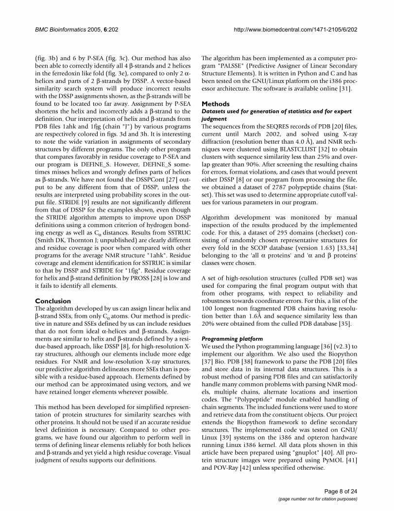
(fig. 3b) and 6 by P-SEA (fig. 3c). Our method has alsobeen able to correctly identify all 4 β-strands and 2 helicesin the ferredoxin like fold (fig. 3e), compared to only 2 α-helices and parts of 2 β-strands by DSSP. A vector-basedsimilarity search system will produce incorrect resultswith the DSSP assignments shown, as the β-strands will befound to be located too far away. Assignment by P-SEAshortens the helix and incorrectly adds a β-strand to thedefinition. Our interpretation of helix and β-strands fromPDB files 1ahk and 1fjg (chain "J") by various programsare respectively colored in figs. 3d and 3h. It is interestingto note the wide variation in assignments of secondarystructures by different programs. The only other programthat compares favorably in residue coverage to P-SEA andour program is DEFINE_S. However, DEFINE_S some-times misses helices and wrongly defines parts of helicesas β-strands. We have not found the DSSPCont [27] out-put to be any different from that of DSSP, unless theresults are interpreted using probability scores in the out-put file. STRIDE [9] results are not significantly differentfrom that of DSSP for the examples shown, even thoughthe STRIDE algorithm attempts to improve upon DSSPdefinitions using a common criterion of hydrogen bond-ing energy as well as Cα distances. Results from SSTRUC(Smith DK, Thornton J; unpublished) are clearly differentand residue coverage is poor when compared with otherprograms for the average NMR structure "1ahk". Residuecoverage and element identification for SSTRUC is similarto that by DSSP and STRIDE for "1fjg". Residue coveragefor helix and β-strand definition by PROSS [28] is low andit fails to identify all elements.

ConclusionThe algorithm developed by us can assign linear helix andβ-strand SSEs, from only Cα atoms. Our method is predic-tive in nature and SSEs defined by us can include residuesthat do not form ideal α-helices and β-strands. Assign-ments are similar to helix and β-strands defined by a resi-due-based approach, like DSSP [8], for high-resolution X-ray structures, although our elements include more edgeresidues. For NMR and low-resolution X-ray structures,our predictive algorithm delineates more SSEs than is pos-sible with a residue-based approach. Elements defined byour method can be approximated using vectors, and wehave retained longer elements wherever possible.

This method has been developed for simplified represen-tation of protein structures for similarity searches withother proteins. It should not be used if an accurate residuelevel definition is necessary. Compared to other pro-grams, we have found our algorithm to perform well interms of defining linear elements reliably for both helicesand β-strands and yet yield a high residue coverage. Visualjudgment of results supports our definitions.

The algorithm has been implemented as a computer pro-gram "PALSSE" (Predictive Assigner of Linear SecondaryStructure Elements). It is written in Python and C and hasbeen tested on the GNU/Linux platform on the i386 proc-essor architecture. The software is available online [31].

MethodsDatasets used for generation of statistics and for expert judgmentThe sequences from the SEQRES records of PDB [20] files,current until March 2002, and solved using X-raydiffraction (resolution better than 4.0 Å), and NMR tech-niques were clustered using BLASTCLUST [32] to obtainclusters with sequence similarity less than 25% and over-lap greater than 90%. After screening the resulting chainsfor errors, format violations, and cases that would preventeither DSSP [8] or our program from processing the file,we obtained a dataset of 2787 polypeptide chains (Stat-set). This set was used to determine appropriate cutoff val-ues for various parameters in our program.

Algorithm development was monitored by manualinspection of the results produced by the implementedcode. For this, a dataset of 295 domains (checkset) con-sisting of randomly chosen representative structures forevery fold in the SCOP database (version 1.63) [33,34]belonging to the 'all α proteins' and 'α and β proteins'classes were chosen.

A set of high-resolution structures (culled PDB set) wasused for comparing the final program output with thatfrom other programs, with respect to reliability androbustness towards coordinate errors. For this, a list of the100 longest non fragmented PDB chains having resolu-tion better than 1.6Å and sequence similarity less than20% were obtained from the culled PDB database [35].

Programming platformWe used the Python programming language [36] (v2.3) toimplement our algorithm. We also used the Biopython[37] Bio. PDB [38] framework to parse the PDB [20] filesand store data in its internal data structures. This is arobust method of parsing PDB files and can satisfactorilyhandle many common problems with parsing NMR mod-els, multiple chains, alternate locations and insertioncodes. The "Polypeptide" module enabled handling ofchain segments. The included functions were used to storeand retrieve data from the constituent objects. Our projectextends the Biopython framework to define secondarystructures. The implemented code was tested on GNU/Linux [39] systems on the i386 and opteron hardwarerunning Linux i386 kernel. All data plots shown in thisarticle have been prepared using "gnuplot" [40]. All pro-tein structure images were prepared using PyMOL [41]and POV-Ray [42] unless specified otherwise.

Page 8 of 24(page number not for citation purposes)

BMC Bioinformatics 2005, 6:202 http://www.biomedcentral.com/1471-2105/6/202

Brief overview of methodologyOur method has five major steps that are used to sequen-tially process the PDB [43] coordinates and assign second-ary structure. These are: 1: Assignment of helix and β-strand propensities to individual residues based on i, i+3Cα distance and i, i+1, i+2, i+3 Cα torsion angle. 2: Delin-eation of probable core regions of helix and β-strand ele-ments from residues that pass strict criteria. 3: Formationof quadruplets of residues connected by two covalent andtwo hydrogen bonds as seeding units for β-sheets. 4: Initi-ation and extension of paired β-strands using quadrupletsof paired residues. 5: Breaking consecutive non-single hel-ices and β-strands taking into consideration residue pair-ing and neighboring elements. Steps of our algorithmneed to be run sequentially for the results to bemeaningful.

Step 1: Assignment of helix and β-strand propensities to individual residuesOur algorithm first conservatively estimates the propen-sity of each residue to be part of a secondary structuralstate (helix, β-strand, both, or none). This is the only stepin which our algorithm deals with secondary structure asa property of the individual residue and not as that of anelement. Cα coordinates of every residue of the moleculeare processed from the N- to C- terminal end and a simpleCα-Cα (i, i+3) distance (fig. 4a) and Cα torsion angle (i,i+1, i+2, i+3) (fig. 4b) are used to mark residues based onwhether they have a propensity to assume helical or β-strand conformation. It is possible for a residue to be partof both a helix and a β-strand, or none of them (coil). Wedecided to use i, i+3 Cα-Cα distances and i, i+1, i+2, i+3 Cαtorsion angles as these parameters have been studiedextensively [7,8,15,21] with regards to their applicabilityto secondary structure definition.

The output of DSSP [8] was used to generate cutoff statis-tics for initial residue-based definition, since it is a con-servative program that delineates secondary structuresbased on hydrogen bonding energy. i, i+3 Cα-Cα distances(fig. 4c) and 4i, i+1, i+2, i+3 Cα torsion angles (fig. 4d)were calculated separately for α-helices and β-strandsfrom DSSP output generated from the "Statset". In thiscalculation, only residues corresponding to the letters 'H'and 'E' in the 'structure' column of DSSP output were con-sidered as helices and β-strands respectively. π, 310-heli-ces, and β-turns were not used as we decided to initiatesecondary structural elements conservatively, using thesecutoffs, and then extend them rather than to start fromspurious elements for later removal.

DSSP [8] provides assignment for individual residues anddoes not assemble them into SSEs. We used DSSP data togenerate elements, and slightly different approaches weretaken for α-helices and β-strands. All consecutive residues

belonging to the helical state were considered as part ofthe same α-helix. For β-strands, DSSP provides bondedpair information (column 'BP1' and 'BP2' in DSSP out-put) and this was used to locate continuous stretches ofpaired residues. Each set of these continuous residues wasconsidered as an element. Distance and torsion angle datawere calculated from the 'N-' to 'C-' terminal end of themolecule. The data was used to determine cutoff condi-tions for identifying potential helix and β-strand-richregions in this step of our algorithm. The followingfunctions were used to decide a particular residue's pro-pensity to form part of helix or β-strand.

δ<8.1 Å, -35°≤τ≤115° ⇒ ρ=loose-helix (1)

δ>8.1 Å, -180°≤τ<-35° | 115°<τ≤180° ⇒ ρ=loose-strand(2)

δ≤6.4 Å, τ within (50.1° ± 2σ) ⇒ ρ=strict-helix (3)

where δ is Cα-Cα distance, τ is Cα torsion angle (i, i+1, i+2,i+3), σ is standard deviation of torsion angle (= 8.6°), ρ ispropensity (cutoff values from figs. 4c, d).

Strict-helix residues thus form a subset of the loose-helixresidues. This eliminates β-bends from interfering withhelix definition even though it also removes π-helices,which have a greater i, i+3 Cα distance than α-helices. Left-handed helices are also removed as they have a lower i,i+1, i+2, i+3 Cα torsion angle than α-helices.

The secondary structure definitions at the end of this stepare in agreement with the findings of several other groupswho have interpreted secondary structures from just theCα coordinates [7,15,17,21]. In our program, we use thisstep as an initial criterion for defining secondary structurestates of individual residues. This definition is furtherrefined and extended in subsequent steps of our programto define SSEs. Estimation of secondary structure of indi-vidual residues is an important step of the algorithm,however the rest of the algorithm is also designed to cor-rect for errors that may have been introduced at this step.

Step 2: Delineation of probable helix and β-strand elementsConsecutive residues with the same secondary structuralpropensity are joined to initiate seed-SSEs. Overlappingelements are considered in this step. The overlap can bebetween elements of the same (H-H, E-E) or different type(H-E, E-H). Since we always process PDB [20] files fromthe N- to the C- terminal end of the polypeptide for gen-erating cutoff data and also generating Cα distance andtorsion angles for this algorithm, extension of seed-SSEsusing the distance and torsion angle data was done from

Page 9 of 24(page number not for citation purposes)

BMC Bioinformatics 2005, 6:202 http://www.biomedcentral.com/1471-2105/6/202

Parameters for assignment of helix and β-strand property to individual residuesFigure 4Parameters for assignment of helix and β-strand property to individual residues. Cα distance and Cα torsion angle were calcu-lated for defining helices (fig. a) and β-strands (fig. b). The distance between residues i, i+3 (shown joined by a blue line) and torsion angle between residues i, i+1, i+2, i+3 (shown as angle between two colored planes; yellow plane between residues i, i+1, i+2 and orange plane between residues i+1, i+2, i+3) are used to assign loose-helix, strict-helix and loose-strand secondary structure property to individual residues. 4c: Distance between i, i+3 Cα residues from helix and β-strand definitions obtained from DSSP [8] output. Distances were binned in 0.2 Å intervals. Cutoff distance c1 (8.1 Å) is the maximum distance allowed for assigning loose-helix property to a residue. Cutoff c1 is also the minimum distance allowed for assigning loose-strand prop-erty to a residue. Residues at i and i+3 positions are allowed in the same SSE template (SSET) only if the cutoff distance c1 passes. Cutoff c2 (6.4 Å) is the maximum i, i+3 Cα distance for strict helix definition. 4d: Torsion angle between i, i+1, i+2, i+3 Cα atoms for helix and β-strand definitions obtained from DSSP output. Angles are binned in 5° intervals. A loose-helix defini-tion is assigned to a residue only if the torsion angle for the residue falls between c1 (-35°) and c2 (115°). A loose-strand is assigned only if the torsion angle is -180° to c1 or c2 to 180°. c3 is the optimal torsion angle for helices and is used to define strict-helix residues if the torsion angle is within a 2 sigma deviation from c3.

Page 10 of 24(page number not for citation purposes)

BMC Bioinformatics 2005, 6:202 http://www.biomedcentral.com/1471-2105/6/202

the C-terminal end of the seed-SSE towards the C- termi-nal end of the polypeptide.

We use a group of at least two consecutive loose-helix res-idues to generate a loose-helix seed-SSE. It is possible toget a single loose-helix residue in β-hairpins whereas a setof consecutive loose-helix residues is more likely to be apart of a helix as it signifies that four (i, i+1, i+3, i+4) res-idues out of a five residue group (i – i+4) have passed cut-offs for i, i+3 Cα distance and i, i+1, i+2, i+3 Cα torsionangle. Loose-helix SSE templates (SSE templatehenceforth referred to as SSET) consisting of at least fiveresidues are formed from every set of consecutive loose-helix residues and the three residues immediately succeed-ing them. This process ensures that a helical element isgenerated from only a single continuous region of loose-helix residues. At this stage, it is possible that the third res-idue of a five residue loose-helix SSET has not passed thecutoffs for distance and torsion angle with any other resi-due. Strict-helix seed-SSE is defined by a group of threeconsecutive strict-helix residues. Strict-helix SSETs areformed from a strict-helix seed-SSE and the three residuesimmediately after it. This implies that every residue in astrict-helix SSET passes the strict cutoffs of distance andtorsion angle with at least one other residue making theminimum length of a strict-helix SSET six residues. Allloose-helix SSETs that do not contain at least one strict-helix residue, other than in the last three residues, are dis-carded. The remaining loose-helix SSETs denote possiblehelix templates.

A loose-strand-forming seed-SSE is defined by a group ofloose-strand residues, with at least one residue in thegroup. Extending every loose-strand seed-SSE to the i+3position at the C- terminal end gives rise to loose-strandSSETs. Overlaps between elements are formed duringextension of the C- terminal end of the seed-SSE to the i+3residue leading to a maximum overlap of two residuesbetween any two SSETs.

Step 3: Quadruplets as seeding units of paired β-strandsIn this step, paired β-strands are generated to identify andrepresent sheet-forming β-strand ladders (including β-bends and β-bridges) which are paired stretches of consec-utive residues. We start by defining and identifying thesmallest unit of such a network of residues, namely aquadruplet, which is formed by four Cα residues, linkedby a pair of covalent bonds and a pair of hydrogen bonds(fig. 5a).

Since the covalent bonds that link a quadruplet of resi-dues are easy to define confidently from their sequenceand coordinates, and their hydrogen bonds are not alwaysclear, we decided to use parameters that depend on cova-lently linked rather than hydrogen bonded residues

neighboring the quadruplet (fig. 5). At most, a single cov-alently linked atom is required from outside the quadru-plet at each of the four corners for calculation ofquadruplet-scoring parameters. DSSP [8] output,obtained from the "Statset" described above, was used toidentify parallel and anti-parallel quadruplets and to scorethe individual parameters that were considered. Only res-idues marked "E" in the DSSP "structure" column andhaving pairs under either or both "BP1" and "BP2" col-umns were used for generation of statistics. The neighbor-ing atoms, if required by the parameter, were also requiredto be marked "E" under the column for "structure". Wedescribe the three parameters used for scoring thequadruplets.

The first parameter Cα-Cα distance between paired resi-dues (fig. 5a), is equivalent to the deviation of vertex i ofthe imaginary triangle i-1, i, i+1 from the vertex j of the tri-angle j+1, j, j-1 (fig. 5b). Cα-Cα distances from binnedDSSP [8] data follow a normal distribution (fig. 5c). Thedistances for parallel and anti-parallel β-strands werecomputed. The distance data were fitted to the followingequations for parallel and anti-parallel quadrupletsrespectively.

where ρ is probability of x, α is a constant, µ is mean andσ is standard deviation. GNUPLOT [40] was used to fit thedata and obtain values for mean (µ) and standard devia-tion (σ).

Probability of obtaining a particular distance, for scoringquadruplets, is calculated by using the mean and standarddeviation obtained above. Two distances are calculatedfor each quadruplet. For parallel quadruplets, both dis-tances are scored individually using the mean and stand-ard deviation from equation 4. For anti-parallelquadruplets, the larger distance is scored using µ2 (c3 infig. 5c) and the smaller distance using µ1 (c2 in fig. 5c),and standard deviation obtained from equation 5 above.Two scores are used for each quadruplet (fig. 5a: distancebetween residues i, j and i+1, j-1).

The second parameter is an angle to determine the devi-ation of a residue pair with respect to the neighboringone. The angle between the line joining potential hydro-gen-bonded residues and the line joining the previousand the next residues of one of the pairing residues wasmeasured, for each of the pairing residues (fig. 5d). Angles

ρ ασ

µσ= × ( )

− −

ex1

22( )

4

ρ ασ

ασ

µσ

µσ1

12 2

12

1 2 2 2

5× + × ( )− − − −

e ex x

( ) ( )

Page 11 of 24(page number not for citation purposes)

BMC Bioinformatics 2005, 6:202 http://www.biomedcentral.com/1471-2105/6/202

The three parameters on which quadruplets scoring is basedFigure 5The three parameters on which quadruplets scoring is based. In figs. a, d, g, a quadruplet is formed from residues i, i+1, j-1 and j. The score is used to select the best quadruplets to join and form β-sheets. Each scoring parameter has been chosen such that they least influence each other. Residues i-1, i+2, j+1 and j-2 are required to calculate angles for quadruplet scoring. The first parameter is Cα-Cα distance between paired residues (fig. a). Blue lines joining i, j and i+1, j-1 show the distance being scored. This parameter approximates the deviation of the triangle apex i with reference to the triangle apex j in fig. b due to rotation of the plane i-1, i, i+1 on the X axis. Fig. c shows the Cα-Cα distances for parallel and antiparallel β-strands obtained from DSSP [8] output. Data is binned at 0.1 Å intervals and fit to a normal distribution using "gnuplot" [40]. Distribution for parallel β-strands has a mean at c1 (4.81 Å) with a sigma of 0.22. Distance for antiparallel β-strands follows a bi-modal distribution with means (µ) at c2 (4.46 Å) and c3(5.24 Å) and a standard deviation (σ) of 0.26. These µ and σ values were used to calculate the probability of occurrence of Cα-Cα pairing distances while scoring quadruplets by our algorithm. A Cα-Cα maximum distance of 7.5 Å (not shown) was used to limit pairing between residues. The second parameter is angle between lines (shown in blue) joining the vertices i, j and the base j-1, j+1 of the imaginary triangles j-1, j, j+1 and i+1, i, i-1 (fig. d). Only one of the four cases is shown. The other angles are between lines j, i and i+1, i-1; j-1, i+1 and i, i+2; i+1, j-1 and j, j-2. Deviation of this angle approx-imates the deviation of the triangle apex i-1 with reference to the triangle apex j+1 in fig. b due to rotation of the plane i-1, i, i+1 on the Y axis. Fig. e shows the distribution of angles, binned at 5° intervals, obtained from parallel and antiparallel β-strands defined by DSSP where c1 (87°) and c2 (82.2°) are the respective means. Fig. f shows the probability of obtaining a parameter-2 angle at different multipliers of the standard deviation for data shown in fig. e. The probability obtained is used for scoring quadruplets. The third parameter is a torsion angle (fig. g) between the points j, mj, mi, i. mj is the midpoint between j+i, j-1. mi is the midpoint between i-1, i+1. Lines joining residues and the midpoints are shown in blue. A similar torsion angle involving residues j-1, i+1 as end points and midpoints between j, j-2 and i, i+2 is computed (not shown). Deviation of the torsion angle approximates the deviation of vertex i in fig. b with respect to vertex j due to rotation of the plane i-1, i, i+1 on the Z axis. Fig. h shows the distribution of torsion angles (binned at 5° intervals) obtained from DSSP output where c1 (-20.9) and c2 (-27.9) are the respective means for data from parallel and antiparallel β-strands. Fig. i shows the probability of obtaining a torsion angle at different multipliers of the standard deviation for the data in fig. h.

Page 12 of 24(page number not for citation purposes)

BMC Bioinformatics 2005, 6:202 http://www.biomedcentral.com/1471-2105/6/202

were measured for parallel and anti-parallel β-strands.Mean (µ; c1 and c2 for parallel and anti-parallel β-strandsrespectively in fig. 5e) and standard deviation (σ) werecalculated from the raw data. Times-sigma deviation wascalculated for each data point (fig. 5f) and the probabilityof obtaining a value at each point was calculated and usedfor scoring quadruplets. Four angles are calculated andscored for each quadruplet (fig. 5d: angle between lines i,j and j-1, j+1; j, i and i+1, i-1; j-1, i+1 and i, i+2; i+1, j-1and j, j-2). From this parameter, only half the total scoreis used to score the quadruplet.

The third parameter is the torsion angle between pairingresidues calculated as an angle between planes joining thepairing residues and the midpoints between the neighbor-ing residues (Fig. 5g: residue j; midpoint mj between resi-dues j+1, j-1; midpoint mi between residues i-1, i+1; andresidue i for the first torsion angle. Residue j-1; midpointbetween residues j, j-2; midpoint between residues i, i+2;and residue i+1 for the second torsion angle.). Angles weremeasured for parallel and anti-parallel β-strands (fig. 5h)and 5a probability vs. times-sigma deviation curve (fig.5i) was prepared similar to that of parameter 2 and usedfor scoring quadruplets. Two torsion angles are calculatedand scored for each quadruplet.

Quadruplet parameters are scored based on the probabil-ity of obtaining individual Z-scores. Deviation of eachparameter data from its respective mean value, obtainedfrom DSSP, is divided by its respective standard deviation,obtained from DSSP, to obtain a Z-score (times-sigmavalue). Probability of obtaining a particular Z-score isused for scoring quadruplets.

As the probability values are very small and could be sub-ject to floating point errors over multiple operations, anegative logarithm was used to convert them to positivenumbers. Thus, lower numbers represent better scores.The total score of the quadruplet is obtained by adding theindividual parameter scores. Equal weights (2 scores forCα distance, half of 4 scores for the second parameterangle and 2 scores for Cα torsion angle) are used for thethree parameters. Technical limitations of the computer'sability to work with numbers close to zero were carefullyavoided by rejecting probabilities close to zero (less thansix decimal places). The table of times-sigma and negativelogarithm of the probabilities were kept for lookup duringscoring of actual quadruplets found by DSSP [8] duringdetermination of quadruplet scoring cutoffs, and by ouralgorithm during β-strand definition.

Sets of true and false quadruplets were generated fromDSSP [8] output (figs. 6a, 6b). A true quadruplet was cre-ated using two pairs of consecutive residues with a link inthe "BP1" or "BP2" column of DSSP output. For every true

quadruplet that was created, four false quadruplets weregenerated as shown in fig. 6 by considering alternativequadruplets that these residues could potentially formwith neighboring residues. Each quadruplet was scoredusing all three parameters (fig. 5) as described above.Scores for true and false quadruplets were analyzed (figs.6c, 6d).

Our algorithm uses quadruplets formed from all availableresidues with the restriction that both covalently linkedresidues do not exist in any strict-helix SSET and allows amaximum overlap of one residue with a strict-helix SSET.Pairing residues are limited by Cα-Cα distance (7.5 Å; fig.5c), before scoring the other two parameters to improvecomputation speed. Since quadruplet-based β-sheet defi-nition is one of the most computationally intensive stepsof the algorithm, we critically examined distance scores toreject quadruplets that will not be part of a β-sheet. Thequadruplets are scored similar to quadruplets obtainedfrom DSSP [8], as described above. Based on the finalscore and cutoffs determined from the scores of true andfalse quadruplets generated from DSSP, quadruplets areplaced in one of three groups. The grade 1 quadruplets arethose with scores better than the best false quadrupletslocated from DSSP in the previous step (quadruplets scor-ing less than c1 in fig. 6c and 6d). The grade 2 quadrupletsare those scoring in between the best false DSSP quadru-plets and worst true DSSP quadruplets (quadruplets scor-ing between c1 and c2 in figs. 6c and 6d). Lastly, the grade3 quadruplets are those, which passed cutoffs of distanceand have non-zero probabilities for each of the threeparameters (fig. 5). These three grades of quadruplets aresorted based on their scores and used as seeding andextending units for all paired β-strands.

Step 4: Calculation of cutoffs to disallow neighboring quadruplets with wrong residue pairingsUse of relaxed criteria such as those described in the pre-vious section to determine the quality of quadruplets canlead to errors in some cases. For example, it is possible toobtain a low scoring grade 1 or a grade 2 quadruplet incases where an extended region comes close to a β-sheet,leading to quadruplets connecting the β-sheet to theextended region. Depending on the local structure, thesequadruplets may score better than those of the β-sheet inthe surrounding region. While it is possible that one or acouple of good hydrogen bonds might actually exist insuch a situation between the β-sheet and the extendedregion, this region will now get incorrectly assigned to thesheet. In such a case, the secondary structure obtained ina residue-correct manner will not be beneficial for the pur-pose of approximating β-sheets as a set of interacting lin-ear elements.

Page 13 of 24(page number not for citation purposes)

BMC Bioinformatics 2005, 6:202 http://www.biomedcentral.com/1471-2105/6/202

A rule based on multi-strand β-sheet geometry was imple-mented to determine correct quadruplet extension andpairing in later steps. True quadruplets generated in theprevious step from DSSP [8] output files (figs. 6a, 6b)were studied with respect to the bending angle of neigh-boring quadruplets having a common pair of covalentlybonded residues. Angles were calculated for each of thecommon pair of residues with its pairs from both quadru-plets (figs. 7a, 7b). An angle of 70° was chosen (c1 in fig.7b) as the cutoff to determine if neighboring quadruplets

are part of the same β-sheet. Both residues of the commoncovalent quadruplet edge have to pass the cutoff for bothneighboring quadruplets to exist in a β-sheet. This ensuresthat no residue in any β-sheet has an angle >70° with itspairs and solves the problem of incorrectly assigning anisolated extended region that happens to be in the vicinityof a sheet as being a part of that sheet.

True and false quadruplets generated from DSSP-defined β-strandsFigure 6True and false quadruplets generated from DSSP-defined β-strands. 6a, 6b: Residues i, j and i+1, j-1 shown paired with green broken lines form the true quadruplet. For every such quadruplet four false quadruplets (shown with red and blue broken lines) are possible: j, i+1, i+2, j-1 and j-1, i, i+1, j-2 in fig. a; i, j-1, j, i-1 and i, i+1, j, j+1 in fig. b. These quadruplets were scored to find the difference in scores between true and false quadruplets. True and false scores for quadruplets generated from DSSP output for parallel β-strand coordinates (fig. c) and antiparallel β-strand coordinates (fig. d). Cutoff c1 (45) and c2 (46) in fig. c are the scores of the best false quadruplet and the worst correct quadruplet respectively for parallel β-strand data. Cutoff c1 (39) and c2 (44) are the scores of the best false quadruplet and worst correct quadruplet respectively from antiparallel β-strand data. Cutoffs c1 and c2 are used as cutoffs to differentiate between grade 1 and grade 2 quadruplets in our algorithm.

Page 14 of 24(page number not for citation purposes)

BMC Bioinformatics 2005, 6:202 http://www.biomedcentral.com/1471-2105/6/202

Initiation and extension of ladders of paired residues using quadrupletsFigure 7Initiation and extension of ladders of paired residues using quadruplets. 7a: Ladders of paired residues are initiated and extended using quadruplets. The initiation quadruplets i+2, i+3, j+5, j+6 and i+6, i+7, j+1, j+2 are shown with green pairing. Quadruplets are attached on either side to extend the arms of the ladder. Addition of quadruplet i+4, i+5, j+3, j+4 joins the two ladders i, i+4, j+4, j+8 and i+5, i+8, j, j+3 to form the complete unit. Depending on the position of the best quadruplets any number of quadruplets might be responsible for seeding a ladder. Smaller ladder fragments get joined by worse scoring quadru-plets. 7b: Residue pairing angle between residues on three β-strands (residue i+1, j-1, k-1 in fig. c) from DSSP output. Cutoff c1 (70°) is close to the largest angle observed. This was used to check new residue pairings formed while adding quadruplets. 7c: Checks performed during quadruplet addition and ladder extension. Quadruplet k, k-1, j-1, j and i, i+i, j-1, j share the common residues j-1 and j. Pairing and angle between pairs are checked for residues j-1 and j when worse scoring quadruplets are added. Quadruplet k, k-1, j-1, j scores better than i, i+1, j-1, j. While adding i, i+1, j-1, j it was found that the angle i, j, k fails the cutoff of 70° (fig. b). Quadruplet i, i+1, j-1, j is not added. Insertion of bulge residues is handled during joining of quadruplets. Quadruplets i+1, i+2, j-2, j-1 and i+2, i+3, j-3, j-2 share the common residues i+2, j-2. The quadruplets are simply added end to end. However, quadruplets j, j-1, k-1, k and j-2, j-3, k-2, k-1 (pairing between j-2, k-1 not shown) share only a single residue k-1. As j-2, j-3, k-2, k-1 scores worse than j, j-1, k-1, k, the pairing between j-1, k-1 is retained and residue j-2 becomes a bulge with respect to residue k-1.

Page 15 of 24(page number not for citation purposes)

BMC Bioinformatics 2005, 6:202 http://www.biomedcentral.com/1471-2105/6/202

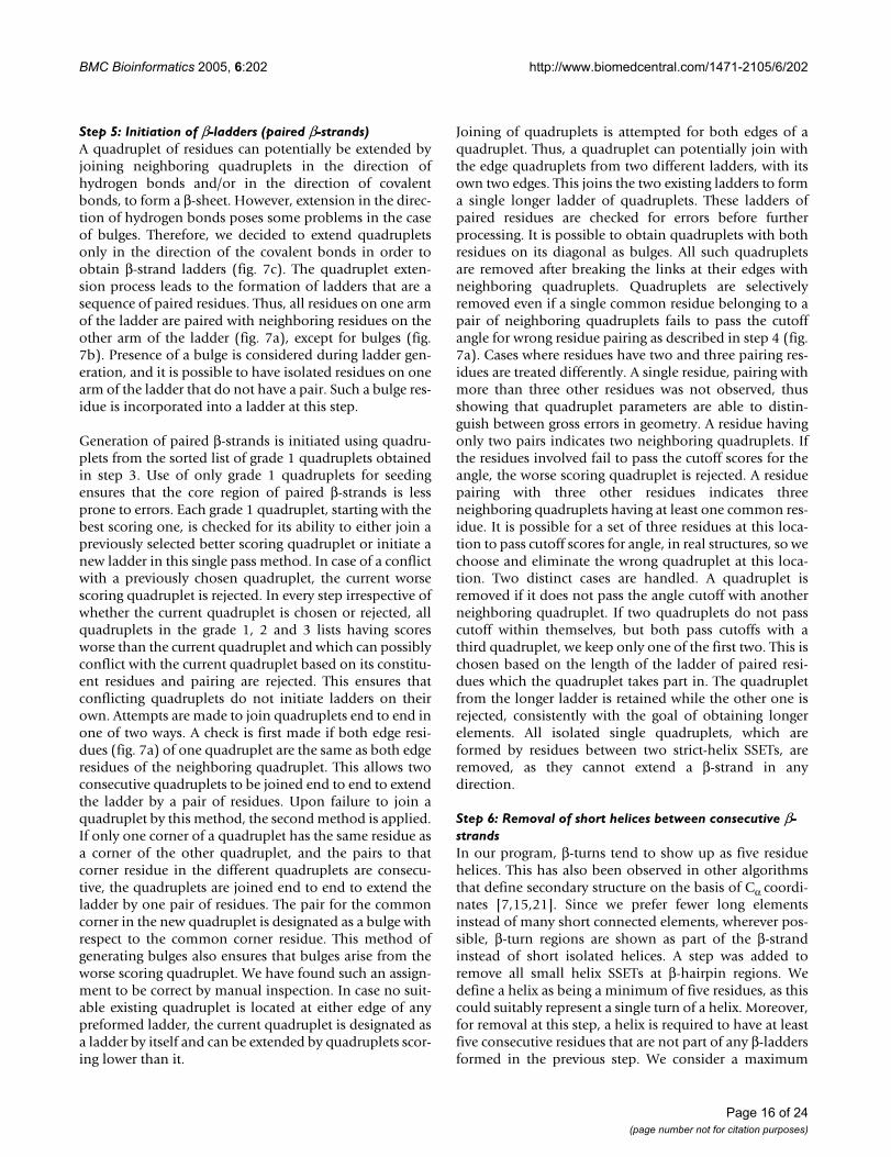
Step 5: Initiation of β-ladders (paired β-strands)A quadruplet of residues can potentially be extended byjoining neighboring quadruplets in the direction ofhydrogen bonds and/or in the direction of covalentbonds, to form a β-sheet. However, extension in the direc-tion of hydrogen bonds poses some problems in the caseof bulges. Therefore, we decided to extend quadrupletsonly in the direction of the covalent bonds in order toobtain β-strand ladders (fig. 7c). The quadruplet exten-sion process leads to the formation of ladders that are asequence of paired residues. Thus, all residues on one armof the ladder are paired with neighboring residues on theother arm of the ladder (fig. 7a), except for bulges (fig.7b). Presence of a bulge is considered during ladder gen-eration, and it is possible to have isolated residues on onearm of the ladder that do not have a pair. Such a bulge res-idue is incorporated into a ladder at this step.

Generation of paired β-strands is initiated using quadru-plets from the sorted list of grade 1 quadruplets obtainedin step 3. Use of only grade 1 quadruplets for seedingensures that the core region of paired β-strands is lessprone to errors. Each grade 1 quadruplet, starting with thebest scoring one, is checked for its ability to either join apreviously selected better scoring quadruplet or initiate anew ladder in this single pass method. In case of a conflictwith a previously chosen quadruplet, the current worsescoring quadruplet is rejected. In every step irrespective ofwhether the current quadruplet is chosen or rejected, allquadruplets in the grade 1, 2 and 3 lists having scoresworse than the current quadruplet and which can possiblyconflict with the current quadruplet based on its constitu-ent residues and pairing are rejected. This ensures thatconflicting quadruplets do not initiate ladders on theirown. Attempts are made to join quadruplets end to end inone of two ways. A check is first made if both edge resi-dues (fig. 7a) of one quadruplet are the same as both edgeresidues of the neighboring quadruplet. This allows twoconsecutive quadruplets to be joined end to end to extendthe ladder by a pair of residues. Upon failure to join aquadruplet by this method, the second method is applied.If only one corner of a quadruplet has the same residue asa corner of the other quadruplet, and the pairs to thatcorner residue in the different quadruplets are consecu-tive, the quadruplets are joined end to end to extend theladder by one pair of residues. The pair for the commoncorner in the new quadruplet is designated as a bulge withrespect to the common corner residue. This method ofgenerating bulges also ensures that bulges arise from theworse scoring quadruplet. We have found such an assign-ment to be correct by manual inspection. In case no suit-able existing quadruplet is located at either edge of anypreformed ladder, the current quadruplet is designated asa ladder by itself and can be extended by quadruplets scor-ing lower than it.

Joining of quadruplets is attempted for both edges of aquadruplet. Thus, a quadruplet can potentially join withthe edge quadruplets from two different ladders, with itsown two edges. This joins the two existing ladders to forma single longer ladder of quadruplets. These ladders ofpaired residues are checked for errors before furtherprocessing. It is possible to obtain quadruplets with bothresidues on its diagonal as bulges. All such quadrupletsare removed after breaking the links at their edges withneighboring quadruplets. Quadruplets are selectivelyremoved even if a single common residue belonging to apair of neighboring quadruplets fails to pass the cutoffangle for wrong residue pairing as described in step 4 (fig.7a). Cases where residues have two and three pairing res-idues are treated differently. A single residue, pairing withmore than three other residues was not observed, thusshowing that quadruplet parameters are able to distin-guish between gross errors in geometry. A residue havingonly two pairs indicates two neighboring quadruplets. Ifthe residues involved fail to pass the cutoff scores for theangle, the worse scoring quadruplet is rejected. A residuepairing with three other residues indicates threeneighboring quadruplets having at least one common res-idue. It is possible for a set of three residues at this loca-tion to pass cutoff scores for angle, in real structures, so wechoose and eliminate the wrong quadruplet at this loca-tion. Two distinct cases are handled. A quadruplet isremoved if it does not pass the angle cutoff with anotherneighboring quadruplet. If two quadruplets do not passcutoff within themselves, but both pass cutoffs with athird quadruplet, we keep only one of the first two. This ischosen based on the length of the ladder of paired resi-dues which the quadruplet takes part in. The quadrupletfrom the longer ladder is retained while the other one isrejected, consistently with the goal of obtaining longerelements. All isolated single quadruplets, which areformed by residues between two strict-helix SSETs, areremoved, as they cannot extend a β-strand in anydirection.

Step 6: Removal of short helices between consecutive β-strandsIn our program, β-turns tend to show up as five residuehelices. This has also been observed in other algorithmsthat define secondary structure on the basis of Cα coordi-nates [7,15,21]. Since we prefer fewer long elementsinstead of many short connected elements, wherever pos-sible, β-turn regions are shown as part of the β-strandinstead of short isolated helices. A step was added toremove all small helix SSETs at β-hairpin regions. Wedefine a helix as being a minimum of five residues, as thiscould suitably represent a single turn of a helix. Moreover,for removal at this step, a helix is required to have at leastfive consecutive residues that are not part of any β-laddersformed in the previous step. We consider a maximum

Page 16 of 24(page number not for citation purposes)

BMC Bioinformatics 2005, 6:202 http://www.biomedcentral.com/1471-2105/6/202

overlap of two residues between elements, so all helices ofeight residues or longer always pass this criterion. Thus forthis step, all helices up to seven residues long are consid-ered for removal. Only helices inside β-hairpin bends asdetected by Cα pairing between the β-strands are removed.

Step 7: Extension of β-laddersQuadruplets with grade two scores are used to extend lad-ders formed from at least two grade 1 quadruplets. All lad-ders therefore have a core region of grade 1 quadruplets,which are then extended to the regions that are more dis-torted. This approximates stretches of paired residues withdefinite hydrogen bonding extended by residues wherestrict hydrogen bonds may be absent, and prevents defin-ing entirely incorrect β-strands. Extension is very similarto the initiation step using grade 1 quadruplets, exceptthat more checks are put in place when each quadruplet isadded, to prevent unreasonably distorted regions frombeing joined. Our algorithm attempts to approximate ele-ments as linear vectors at every step of the process. Weincorporated steps to geometrically define the end of aladder of paired residues to prevent generating laddersthat span more than a single linear element. Quadrupletsare not added if these criteria are violated. As grade 2quadruplets are formed using less stringent criteria thanthe grade 1 quadruplets, a conservative approach in theiruse prevents delineation of highly distorted regions as β-strands. Extension is attempted on a list of ladders sortedby length. This ensures that longer elements have a betterchance of ending due to geometric criteria rather than dueto an extension quadruplet already being allocated to ashorter ladder. A pair of residues are added to the ladderonly if neither of the new residues already have two otherresidue pairs each. Thus, ladder extension depends bothon ladder length as well as on quadruplet grade. Extensionof a ladder is also terminated if this causes residue overlapwith residues already participating in a strict-helix SSET.Only residues that are a part of a loose-strand SSET areused in the extension step. Extension is also terminatedupon reaching a β-hairpin bend. No residues are added ifthe pair about to be added does not fall within the dis-tance cutoffs of 3.5 Å to 7.5 Å (fig. 5a). The ladder is ter-minated, if any of the residues about to be added have ani-3, i Cα-Cα distance less than 8.1 Å (eq 1, fig. 4c) with aresidue already in the same ladder. This ensures that wedo not extend a ladder over a β-bend.

Grade 3 quadruplets are used next, to extend only singlegrade 1 quadruplets that have not been extended by anyof the above methods. As grade three quadruplets are theworst scoring quadruplets that are used, two importantconstraints are utilized to prevent spurious extensions oflone grade 1 quadruplets. Firstly, we decided to use a cri-terion of exactly three consecutively paired residues todenote paired β-strands that arose from single grade 1

quadruplets. This ensures that only a single unreliablegrade 3 quadruplet is used for extension of any particularβ-ladder. Upon inspection of structures, it was observed inthat keeping a minimum of two consecutively paired res-idues, namely a single grade 1 quadruplet, to delineate β-strands, was too relaxed. This constraint alone was able toeliminate most cases of chance interaction between pairsof residues. However, in highly distorted regions that aretoo twisted to represent linear elements, more than a pairof consecutive residues seem to form isolated ladders. Wedecided not to include them as well. So, secondly, onlygrade 1 quadruplets sharing common residues with anexisting β-ladder, formed by previous initiation andextension steps, are extended by a single grade 3 quadru-plet, such that it maintains residue pairing with the longerβ-ladder. These two constraints together ensure that weretain short, three residue, β-strands at edges of existing β-sheets even if they are slightly distorted, but at no otherregion unless they are initiated by a pair of consecutivegrade 1 quadruplets.

At this stage, due to the possibility of bulges at the over-lapping edges of consecutive β-ladders, we might obtainconsecutive ladders of residue pairs whose one arm is sep-arated from the other by a single residue. These ladders arejoined with a single bulge residue if consecutive pairingarms on the other side share a common residue andrestrictions imposed during ladder extension are not vio-lated. Our method of ladder generation also makes it pos-sible to obtain overlapping ladders such that one arm ofone ladder overlaps with the arm of a different ladder.Due to the complicated nature of β-sheets, it is also possi-ble to not have residue pairing between neighboring β-strands in the middle of a β-sheet. Dealing with multiplefragments of overlapping ladder-arms prevents the abilityto distinguish between true edges of β-strands. Thus, wejoin all ladder arms that are formed from consecutivestretches of residues or with common residues betweenthem. These joined ladder arms are used to denote β-strands. The residue pairing information generated duringladder formation is retained to generate pairing informa-tion between the newly formed β-strands. Consistent withour minimum requirement of three pairing-residues forladders (described above), β-strands are considered aspart of the same β-sheet if at least three residues arepaired.

Step 8: Generating and breaking α-helices to form linear elementsHelix SSETs representing α, π and 310-helices, defined inthe above steps, are based on relaxed criteria to avoidmissing out residues that could potentially be part of ahelical element. Although a rudimentary form of elementedge delineation is obtained by the use of Cα distance andtorsion angles during delineation of probable helical ele-

Page 17 of 24(page number not for citation purposes)

BMC Bioinformatics 2005, 6:202 http://www.biomedcentral.com/1471-2105/6/202

ments in step 2, these methods are capable of detectingonly drastic changes in the helix axis. Our relaxed criteriaof helix definition designed to include π and 310 helices,also allows curved, kinked and bent helices [44] to beincluded as being a part of a single element. In order toapproximate these elements by vectors suitable for motifsearch, we decided to split these helices into linear ele-ments while considering overlap between them. Somehelix SSETs are found to overlap with parts of ladders gen-erated and extended in the previous step. As the residuesthat overlap are not part of strict helix SSETs we prefer astate of 'β-strand' to 'α-helix' for the residues. Helix SSETshaving β-strand overlaps are checked and shortened so asnot to have more than two residue overlap, and only atthe edges, with any residue that is part of a β-strand. As itis possible for a residue to form only two hydrogen bonds,we simulate this constraint by rejecting from the edge ofthe helix any residues that pair with more than one otherresidue in the formation of β-strands in the above step.The helices are again checked for the presence of at leastfive residues before being accepted for processing by thisstep.

Manual judgment of the results at this point indicated thatour program's delineation of helices were acceptable interms of residue coverage. Presence of bent helices wasnoticed in the checkset (described previously) and wedecided to split them into linear elements without loss ofconstituent residues. We used helices defined by our pro-gram for calculation of parameters for breaking helices.Since DSSP [8] does not distinguish between consecutivehelices, it was not possible to derive parameter-based cut-offs from DSSP helix definition. Using data from helicesdefined by our program, enabled us to implement a sys-tem that could properly handle loosely defined helicesand not to break them more frequently than needed. Theresults were visually inspected for errors.

The helix breaking method relies on an analysis of theRMSD of helix residues around the helix axis. Twodifferent methods were used to generate the helix axis.Only one of the methods was finally adopted (fig. 8a). Weexplain both methods, as they are equally suitable forlong (>7 residue) α-helices. However, the method chosenfor our algorithm works for helices defined by us whichencompass α, π and 310 helices as distinct or part of thesame element and also short (<8 residue) α-helices. Thefirst method calculates the principal moment of the helixresidues and used the eigenvector corresponding to thelargest eigenvalue as the helix axis. This method thusdepends only on the spread of the residues in space anddoes not take into account the linear connectivity of thehelix residues. Errors in helix axis assignment wereobserved for π-helices and short α-helices. Due to thespread of residues being more on the diametrical plane of

these helices, the axis found using the eigenvector methodlay closer to the plane of the diameter instead of beingnormal to it. This method gave good results for longer hel-ices. However, as we considered short α, π and otheropened up helices for breaking and final definition, thismethod was not used.

Based on the observations above, a rotational fit methodwas used to determine helix axis [22,45] (fig. 8a). Thisinvolves shifting the helix by one residue and aligning itwith the original helix. The rotation axis corresponds tothe helix axis. This was found to precisely determine thehelix axis and was not dependent upon the length orunder-winding of the helix. The axis determined by thismethod and that determined by the eigenvector methodcorrelate very well for helices greater than 8 residues (datanot shown).

Our program was run on the "statset", described previ-ously, and all helices were extracted for study. The RMSDof helix residues from the helix axis were calculated andanalyzed (fig. 8b). All helices were processed using thehelix-breaking method described below. Each helix wassplit in three ways such that case 1 gave rise to 2 pieces,case 2 gave rise to 3 pieces and case 3 gave rise to 4 piecesfrom the original unbroken helix. The mode of breakingangles was calculated for every helix length (data notshown). The highest mode (22°) obtained was used inour breaking method to obtain a set of all helices thatbroke at least once at an angle greater than the mode. Bro-ken helices that arose from this set were used to calculatethe RMSD of broken helices around the rotational fit axis(fig. 8a). The standard deviation was calculated for everyhelix length and the results showing dependency of thestandard deviation on the length were fitted to a straightline (data not shown).

The average RMSD and average standard deviation calcu-lated above were used to obtain broken helices (asdescribed below) that were analyzed manually. Our algo-rithm does not break a helix showing a slight curvature inits structure, or containing a few distorted residues. Forbent helices, we decided to use two cutoffs to determinebreakpoints. Flexibility is represented by a Z-score repre-senting the allowed deviation as multiples of the standarddeviation of helix residues (as calculated above). A sharpbend in the helix axis is measured by the angle betweenthe axes of two neighboring helices as calculated by therotational fit method (described above). The broken heli-ces observed were manually inspected to determine theoptimum Z-score and the break angle (fig. 8c).

A breaking method for helices was developed in order todetermine the correct cutoffs for Z-score and angle ofbreak. The method considers every possible breakpoint in

Page 18 of 24(page number not for citation purposes)

BMC Bioinformatics 2005, 6:202 http://www.biomedcentral.com/1471-2105/6/202

Helix endpoints redefined based on RMSD and angle between their axial vectorsFigure 8Helix endpoints redefined based on RMSD and angle between their axial vectors. 8a: Vectors representing a short opened up helix by two different methods. The red arrow shows the axis obtained by using the largest spread of the Cα atoms (vector corresponding to the largest eigenvalue). The green arrow shows the rotational axis obtained when the helix that is shifted by one residue, is aligned to the original helix. The first method is unsuitable for representing this helix and does not work for π and short helices. Our algorithm uses the rotational-fit method (described below, 8b) for all helices. RMSD of residues are cal-culated over this vector. Angles between vectors, calculated from residues of consecutive helices, are used to determine whether to break them so as to appropriately define the helices as linear elements. 8b: Helix RMSD data calculated using the rotational fit vector. Average RMSD of unbroken helices from our algorithm varies widely. The helices were broken multiple times and the angle of break was analyzed (data not shown). The mode of the angle of break (22°) for long (>15 residue) heli-ces was used to determine the break point of consecutive helices. Helices that break at >22° were chosen for the dataset for calculation of RMSD and angle of break (fig. c). Average RMSD of broken helices is shown in this figure. A line was fitted using "gnuplot" [40] to approximate the RMSD of broken helices. A Z-score of 2.5 is used to limit breaking helices that deviate less than 2.5 times sigma around the approximated RMSD value for broken helices at a particular helix length. 8c: Angle of helix break calculated from dataset of helices used in fig. b. Data were collected from helices broken once, twice and thrice. The normalized data are shown. Helices that show an angle greater than c1 (20°) between broken parts are split. 8d: Helix split by our algorithm. All possibilities of broken pieces are assessed with respect to the RMSD of the pieces and angle of break. Heli-ces i, i+5 and i+4, i+15 are finally chosen as correctly broken. Helices i, i+8 and i+15; and i, i+11 and i+10, i+15 are also possi-bilities that are analyzed but not chosen as the optimum break. Residues i+4, i+5 are shared by the two helix pieces (Cα shown as spheres).

Page 19 of 24(page number not for citation purposes)

BMC Bioinformatics 2005, 6:202 http://www.biomedcentral.com/1471-2105/6/202

a helix and attempts to choose the optimal result. Wedefine broken helices as single elements only if the piecewith the highest RMSD is still acceptable (fig. 8d). Multi-ple breaks are considered with no overlaps and with over-laps of up to two residues at every position of the helix.The minimum helix length allowed is five residues. Bro-ken helices are considered starting from the shortest helixlength (5 residues), with maximum overlap (2 residues),to the longest possible helix (the unbroken helix). Thehelix breaking process analyses the RMSD and angle ofbreak for every combination of helical fragments(instance) derived from the unbroken helix. Thus, every"instance" is the set of broken helical fragments producedduring the iterative breaking process. Every possible caseof broken helices that can be formed by an unbroken helixis considered and a single helix is broken into as manylong fragments as is optimal for correct representation aslinear elements. RMSD along the helix axis, computed bythe rotational fit method described above, is used to deter-mine overall suitability of broken helical pieces. For everyunbroken helix, RMSD of every possible broken helicalfragment is considered. For all "instances" of broken heli-ces, the fragment with the highest RMSD is located. The"instance" where the highest RMSD is minimum is con-sidered the optimum break. Thus, we aimed to minimize,over all possibilities in which a single helix may be bro-ken, the maximum RMSD of the broken helices generatedby a single "instance". A Z-score cutoff is used to deter-mine if a helix or helix-fragment needs to be broken. Wetried out different values of Z-scores in an attempt to findthe optimum value. The results for every set of broken hel-ices corresponding to different Z-scores were manuallyinspected to disallow breaking helices that looked like asingle element. Consecutive fragments are treated as a sin-gle helix if the angle between their axes is less than the cut-off angle, even if the resulting helix has a Z-score that failscutoffs. A Z-score cutoff of 2.5 and an angle cutoff of 20°(fig. 8c) were finally chosen. Results were judged manu-ally for correctness. Linear helices, according to our algo-rithm, thus never fail the axial bending angle of 20° andare not broken. This is close to the 25° angle obtained byKundrot and Richards [15]. Curved helices are brokenonly if they are long and the axial bending angle is above20°. Bent and kinked helices are already broken in step 2(by i, i+3 Cα distance and i, i+1, i+2, i+3 Cα torsion cutoffs;fig. 4c, 4d) as they have a sharp angle and never need tobe broken by this step.

This step of the calculation is computationally intensivedue to the large number of possibilities that are consid-ered. To prevent the algorithm from taking abnormallylong to complete in special cases, we avoid checking forbreaks in single helices that are longer than 50 residues.

Step 9: Breaking β-strands to generate linear elementsBent β-strands are split to obtain linear elements usingboth geometric criteria (Cα distance and angle) and byusing neighbor pairings for constituent residues. As β-strands have a natural tendency to curve, we take care notto break short gently curved β-strands, nor break them atbulges. Sharp bends in β-strands, gently curved but longβ-strands, which cannot be optimally represented by asingle linear vector, and β-strands which do not have atleast two residues shared by two different β-sheets are con-sidered for breaks. β-strands are broken using geometriccriteria after checking for the possibility of a bulge beinglocated near the potential breakpoint. We prefer to retainlarge regions of connected β-strands rather than split theminto isolated pieces, and therefore place more importanceon residue pairings than on geometric criteria of individ-ual β-strands. Restricting the minimum length of a β-strand to three residues (as described above) makes β-strand breaking a sensitive operation, as it is possible tolose small β-strands completely if breaks are located eitherwithin the small β-strands themselves or on the β-strandpairing with the small β-strand. Thus, we try to retain res-idues in short β-strands if they are linked to part of a largerβ-sheet. However, it is more likely for short β-strands toarise due to chance proximity of extended regions. Theseshort β-strands may hinder correct representation of theentire β-sheet. Although our program does not aim to per-fectly describe β-sheets, we do try to detect and removeshort β-strands that are either not well connected to alarger β-sheet or located close to breaks in neighboring β-strands of the β-sheet. The β-strand breaking methods aredesigned not to depend on the length of the β-strandsbeing broken, however, they do depend on the order inwhich they are applied on the original β-strand and itspaired neighbors. β-Strands are broken in four steps,where each step works on the complete set of β-strandsobtained after applying the previous breaking method.Bulges are taken into consideration at every step.

β-hairpin regions of β-strands are broken first, and thesebreaks are permanent. The use of quadruplets to generateβ-ladders and joining ladder-arms to obtain paired β-strands does not allow demarcation of β-hairpin regionsperfectly. Also, use of β-hairpin residues to form part of β-ladders in previous steps is not consistent with our aim ofusing a quadruplet to represent pairs of hydrogen bondedresidues, since the last pair of residues of a hairpin bendmay be consecutive and thus covalently bonded. Further,residues of hairpin bends, even when separated by a singleresidue score low when included in quadruplets. We iden-tify all β-hairpins using residue pairing. This enables β-hairpin identification even if the last pair of paired resi-dues leading to the hairpin is separated by up to three res-idues. This method allows detection of a β-hairpincorrectly if the β-hairpin residues are paired with neigh-

Page 20 of 24(page number not for citation purposes)

BMC Bioinformatics 2005, 6:202 http://www.biomedcentral.com/1471-2105/6/202

boring β-strands but not between themselves. All suchcases of β-hairpins are resolved by placing the residues inone of the two β-strands based on residue pairing of con-secutive residues. In case of an odd number of residuesbeing in the β-hairpin, the middle residue is left out of theβ-strands on either side of the β-hairpin.

Geometric breaks of β-strands using i, i+3 Cα-Cα distanceare considered (fig. 9a). These account for the presence ofbulges and are not marked as permanent breakpoints.Depending on pairing of and breakpoints in neighboringβ-strands, the breakpoint may be disregarded in latersteps. If the i, i+3 Cα distance is less than the cutoff of 8.1Å (c1 in fig. 4c) a break is inserted. Presence of a bulge,originating from β-ladder initiation and extension stepsabove, within any of the residues at i, i+1, i+2, i+3 posi-tions, prevents a break. The residues at positions i+1 andi+2 are treated as overlapping residues and included inboth β-strands. Although breaks generated by this methodindicate structurally bent regions, they are discarded uponabsence of other potential breakpoints in the vicinity, atlater steps. Breaks are not initiated if they lead to less thanthree-residue long β-strands.

Geometric breaks of β-strands are also considered basedon i-1, i, i+2 Cα angle. The i ± 2 Cα angle was observed tobe a reliable indicator of bent β-strands in non-bulgeregions. This break, as in the previous case, is treated as apotential break point only. A permanent break is initiatedonly if no bulges are observed in the β-strand region. Allβ-strands defined by our program were extracted fromPDB [20] chains in the "statset" and the i-2, i, i+2 angleswere calculated (fig. 9b). An angle of 45° (c1 in fig. 9b)was used as cutoff to determine a breakpoint. This wasfound to be too restrictive in that regions with only a sin-gle distorted residue could get broken. A method wasimplemented to locate β-strand distortions in the sur-rounding region using a less restrictive criterion. Data forfinding cutoffs for bulge detection was found by process-ing the "statset" with our program. All β-strands definedby our program were extracted. A pseudo point was cre-ated for each set of four consecutive residues belonging tothe same β-strand using residues i-1, [i, i+1, i+2, i+3], i+4(fig. 9c). The angle between the lines joining the pseudo-point to the residues before and after the four residuesused for the pseudo-point was calculated for all residuesof the β-strands (fig. 9b). An angle cutoff of 70° (c2 in fig.9b) was chosen to allow gradual bends in the structure. Abreak is allowed only if the i-2, i, i+2 Cα angle and thepseudo-point angle both fail for a given residue i. Breaksare not initiated if they lead to β-strands less than threeresidues long.

The final method used for β-strand breaking considers res-idue pairing between β-strands. Using residue pairing for

detecting the end positions of β-strands allows splitting aβ-sheet correctly based on the whole structure and not onminor distortions in geometry. Breaks by this method arepermanent and are used as deciding factors in splitting anentire β-sheet into smaller pieces. Although our programdoes not aim to produce a perfect definition of all β-sheets, with respect to their boundaries as appropriate forcorrect domain definition, we do verify the SSE pairings toinclude them as part of the correct β-sheet. Due to the wayin which ladders of residue pairs (described previously)were generated and joined, it is possible for two ladderarms to be formed from consecutive residues or be with amaximum of only one residue common between them,with the residues on the other arms having no connectiv-ity (fig. 9d). A minimum of two residues overlap isrequired for neighboring β-strands to be part of the sameβ-sheet. Thus, a break is initiated if residues of a β-strandpairing with one of its neighbors lose contact with it formore than a single residue, unless the other pairing β-strand continues to maintain residue pairing on the otherside. Only one common residue is allowed at the break,thus allowing a single residue to pair with both the neigh-bors, which are placed in different β-sheets. A β-strand isnot considered for breaks if there are at least two residuespairing with both neighboring β-strands. Flexibility inallowing lost contact for a single residue ensures thatbulges are retained.

Step 10: Generation of helices from residues not in any elementIn previous steps, residues not part of a strict-helix SSETwere considered for generation of ladders of residue pairsand β-strands. Some of these residues do not finally par-ticipate in any β-strand formation. These residues, notpart of α-helices or β-strands, can potentially contribute toformation of π and 310 helices, or may be distorted whilestill showing helical tendency. Overlap with previouslydefined α-helices and β-sheets were considered for thisstep.

All loose-helix SSETs having no residue in a previouslydefined α-helix or a β-strand are considered at this step.To loosen the criteria and to allow over and under-woundhelices to be detected, any presence of a strict helix-form-ing residue, other than in the last three residues of the pre-viously defined element, leads to rejection of the templatefrom consideration, as these have already been consideredfor helices in above steps. The templates are checked for amaximum overlap of two residues with β-strand elementsand shortened at the edges if required. The templates arealso checked so that no residue overlapping with a β-strand at the edge, pairs with more than one β-strand res-idue. Finally, helix templates occurring at β-hairpins areremoved. Any helix template that overlaps with β-strandson both edges and has less than five non-overlapping

Page 21 of 24(page number not for citation purposes)

BMC Bioinformatics 2005, 6:202 http://www.biomedcentral.com/1471-2105/6/202

β-strands redefined to obtain linear elements using different methodsFigure 9β-strands redefined to obtain linear elements using different methods. 9a: Strands broken based on i, i+3 Cα distance (fig. 4a). Distance between i-1, i+2 residues and i+13, i+16 residues fail the cutoff distance of 8.1 Å. The residues i, i+1 (shown in red) are shared by β-strands i-9, i+1 and i, 1+7. Residues i+15, i+14 (shown in red) are shared by the β-strands i+24, i+14 and i+15, i+8. 9b: Angles for β-strand breaking while accounting for bulges. Angles were calculated from all β-strands defined by our algorithm before the β-strand-breaking step. The angle between i-2, i, i+2 Cα atoms is used to determine if the β-strand is bent. An average pseudo-point (pp) was generated from the j, j+1, j+2, j+3 atoms and the angle between j-1, pp, j+4 was found. β-strands were broken when i-2, i, i+2 angle was greater than c1 (45°) and j-1, pp, j+4 angle was greater than c2 (70°). j = i-1 showed the best correlation between the two angles (data not shown). 9c: Strand breaking using pseudo-point to find dis-torted regions. Residues i-1, i, i+1, i+2 (shown in red) are used to generate an average point. Angle between i-2, the average point and i+3 locates a distorted region if the cutoff angle of 70° fails. The β-strand is broken if the i-2, i, i+2 angle also fails at the same location. The β-strand i-3, i+4 is split to generate two β-strands i-3, i+1 and i, i+4. 9d: Strand breaking using pairing information between neighboring β-strands. Residue i (shown in red) is paired to residue j on one side and to residue k on the other. Residue i+1 is paired to residue j-1 however residue i-1 is not paired to β-strand j. Also, residue i-1 is paired to residue k+1 but residue i+1 is not paired to β-strand k. Lack of a pair of common residues pairing between β-strand j and k splits the sheet, with residue i shared between both sheets.

Page 22 of 24(page number not for citation purposes)

BMC Bioinformatics 2005, 6:202 http://www.biomedcentral.com/1471-2105/6/202

helix residues is rejected. All remaining loose-helix SSETsare included in our final helix definition.

Step 11: Assignment of β-strands to β-sheetsAs described previously, we consider a minimum of twopairs of residues to determine linked β-strands whichthemselves are at least 3 residues long. Consecutiveresidues of β-hairpins are considered linked for this pur-pose, even though they do not actually form a hydrogenbond. Sheets are assigned for each group of β-strands thatcan be traversed by a consecutive pair of linked residues.Breaks in β-strands located in previous steps are taken intoconsideration for this step. Breaks caused by changes inpairing (described previously) are treated as permanent,and the β-strands on either side are kept in separate β-sheets. Breaks caused by geometric evaluation of the localregion are treated as potential breaks. A geometric break isignored unless it affects all paired residues on either sideof it. Thus, geometric breaks are used only if multiple β-strands need to be broken to split the β-sheet. Keeping arigid criterion for the use of geometric breaks forindividual β-strands ensures flexibility for the entire β-sheet, as larger β-sheets tend to show a gradual bending. Amore drastic bending shows up as a sequence of geometricabnormalities, thus allowing proper use of the potentialgeometric breaks detected previously.

Assignment of β-strands to β-sheets is for ease of motifsearches only. Our program does not define β-sheets forthe purpose of domain definition. As such, ambiguityregarding whether two β-sheets should be linked or sepa-rate might arise in cases where there is a gradual bendingof the sheet or where two or more β-strands link them atthe edges. It is also possible for two different β-sheets tobe linked together if a few β-strands in each sheet are dis-torted and are in close proximity to each other. In themajority of cases, however, our program defines β-sheetboundaries correctly.

Robustness of secondary structure assignment towards coordinate errorsRobustness towards coordinate errors was estimated bychecking consistency of definition using randomly shiftedPDB [20] coordinates. Gaussian random numbers wereused to shift coordinates of the 100 files in the culled PDBset. Every residue (all atoms together) was individuallyshifted in all the three axes. 100 randomly shifted coordi-nate files were generated for every PDB file, starting eachtime with the original coordinates. 10 sets of 10,000 fileseach were generated with average RMSD from 0.2Å to2.0Å in steps of 0.2Å. Secondary structure definition pro-duced by DSSP [8], P-SEA [17] and our algorithm for eachof these 1,00,000 files was compared with the definitionproduced by the same program from the unaltered coor-dinates. Mean percentage of correct definition over all res-

idues, assuming definition from the unaltered definitionto be fully correct, and standard error was calculated foreach set of 10,000 files for each program (fig. 2a). Meanpercentage of total residues reported as helices and β-strands for each of these 10 sets were also noted (fig. 2b).

Authors' contributionsIM designed and implemented the algorithms, tested pro-gram performance, analyzed the results, and drafted themanuscript. SSK contributed to algorithm developmentand provided expert judgment of program output. NVGconceived of the study and participated in its design andcoordination. All authors read and approved the finalmanuscript.

AcknowledgementsThis project was supported by NIH grant GM67165 to NVG. We thank James O. Wrabl for reading the manuscript and providing valuable comments.

References1. Pauling L, Corey RB: Configurations of polypeptide chains with

favoured orientations around single bonds: two new pleatedsheets. Proc Natl Acad Sci U S A 1951, 37:729-740.

2. Donohue J: Hydrogen bonded helical configurations of thepolypeptide chain. Proc Natl Acad Sci U S A 1953, 39:470-478.

3. Low BW, Grenville-Wells HJ: Generalized mathematical rela-tionships for polypeptide chain helices. The coordinates ofthe pi helix. Proc Natl Acad Sci U S A 1953, 39:785-802.

4. Venkatachalam CM: Stereochemical criteria for polypeptidesand proteins. V. Conformation of a system of three linkedpeptide units. Biopolymers 1968, 6:1425-1436.

5. Rose GD, Gierasch LM, Smith JA: Turns in peptides and proteins.Adv Protein Chem 1985, 37:1-109.

6. Richardson JS: The anatomy and taxonomy of proteinstructure. Adv Protein Chem 1981, 34:167-339.

7. Levitt M, Greer J: Automatic identification of secondary struc-ture in globular proteins. J Mol Biol 1977, 114:181-239.

8. Kabsch W, Sander C: Dictionary of protein secondary struc-ture: pattern recognition of hydrogen-bonded and geometri-cal features. Biopolymers 1983, 22:2577-2637.

9. Frishman D, Argos P: Knowledge-based protein secondarystructure assignment. Proteins 1995, 23:566-579.

10. King SM, Johnson WC: Assigning secondary structure fromprotein coordinate data. Proteins 1999, 35:313-320.

11. Sklenar H, Etchebest C, Lavery R: Describing protein structure:a general algorithm yielding complete helicoidal parametersand a unique overall axis. Proteins 1989, 6:46-60.

12. Colloc'h N, Etchebest C, Thoreau E, Henrissat B, Mornon JP: Com-parison of three algorithms for the assignment of secondarystructure in proteins: the advantages of a consensusassignment. Protein Eng 1993, 6:377-382.

13. Taylor WR: Defining linear segments in protein structure. JMol Biol 2001, 310:1135-1150.

14. Oldfield TJ, Hubbard RE: Analysis of C alpha geometry in pro-tein structures. Proteins 1994, 18:324-337.

15. Richards FM, Kundrot CE: Identification of structural motifsfrom protein coordinate data: secondary structure and first-level supersecondary structure. Proteins 1988, 3:71-84.

16. Dupuis F, Sadoc JF, Mornon JP: Protein secondary structureassignment through Voronoi tessellation. Proteins 2004,55:519-528.

17. Labesse G, Colloc'h N, Pothier J, Mornon JP: P-SEA: a new effi-cient assignment of secondary structure from C alpha traceof proteins. Comput Appl Bio Sci 1997, 13:291-295.

18. Mizuguchi K, Go N: Comparison of spatial arrangements ofsecondary structural elements in proteins. Protein Eng 1995,8:353-362.

Page 23 of 24(page number not for citation purposes)

BMC Bioinformatics 2005, 6:202 http://www.biomedcentral.com/1471-2105/6/202

Publish with BioMed Central and every scientist can read your work free of charge

"BioMed Central will be the most significant development for disseminating the results of biomedical research in our lifetime."

Sir Paul Nurse, Cancer Research UK

Your research papers will be:

available free of charge to the entire biomedical community

peer reviewed and published immediately upon acceptance

cited in PubMed and archived on PubMed Central

yours — you keep the copyright

Submit your manuscript here:http://www.biomedcentral.com/info/publishing_adv.asp

BioMedcentral

19. Hutchinson EG, Thornton JM: PROMOTIF--a program to iden-tify and analyze structural motifs in proteins. Protein Sci 1996,5:212-220.

20. Berman HM, Battistuz T, Bhat TN, Bluhm WF, Bourne PE, BurkhardtK, Feng Z, Gilliland GL, Iype L, Jain S, Fagan P, Marvin J, Padilla D, Rav-ichandran V, Schneider B, Thanki N, Weissig H, Westbrook JD, Zard-ecki C: The Protein Data Bank. Acta Crystallogr D Biol Crystallogr2002, 58:899-907.

21. Ramakrishnan C, Soman KV: Identification of secondary struc-tures in globular proteins--a new algorithm. Int J Pept ProteinRes 1982, 20:218-237.

22. Bansal M, Kumar S, Velavan R: HELANAL: a program to charac-terize helix geometry in proteins. J Biomol Struct Dyn 2000,17:811-819.

23. Ramachandran GN, Sasisekharan V: Conformation of polypep-tides and proteins. Adv Protein Chem 1968, 23:283-438.

24. Laskowski RA, Rullmannn JA, MacArthur MW, Kaptein R, ThorntonJM: AQUA and PROCHECK-NMR: programs for checkingthe quality of protein structures solved by NMR. J Biomol NMR1996, 8:477-486.

25. DePristo MA, de Bakker PI, Blundell TL: Heterogeneity and inac-curacy in protein structures solved by x-ray crystallography.Structure (Camb) 2004, 12:831-838.

26. Webber CLJ, Giuliani A, Zbilut JP, Colosimo A: Elucidating proteinsecondary structures using alpha-carbon recurrencequantifications. Proteins 2001, 44:292-303.

27. Carter P, Andersen CA, Rost B: DSSPcont: Continuous second-ary structure assignments for proteins. Nucleic Acids Res 2003,31:3293-3295.

28. Srinivasan R, Rose GD: A physical basis for protein secondarystructure. Proc Natl Acad Sci U S A 1999, 96:14258-14263.

29. Ichikawa S, Hatanaka H, Yuuki T, Iwamoto N, Kojima S, Nishiyama C,Ogura K, Okumura Y, Inagaki F: Solution structure of Der f 2, themajor mite allergen for atopic diseases. J Biol Chem 1998,273:356-360.

30. Carter AP, Clemons WM, Brodersen DE, Morgan-Warren RJ, Wim-berly BT, Ramakrishnan V: Functional insights from the struc-ture of the 30S ribosomal subunit and its interactions withantibiotics. Nature 2000, 407:340-348.

31. PALSSE [http://prodata.swmed.edu/palsse/]32. Wolf YI, Dondoshansky I: BLASTCLUST. [http://

www.ncbi.nlm.nih.gov/Web/Newsltr/Spring04/blastlab.html].33. Murzin AG, Brenner SE, Hubbard T, Chothia C: SCOP: a structural

classification of proteins database for the investigation ofsequences and structures. J Mol Biol 1995, 247:536-540.

34. Lo Conte L, Ailey B, Hubbard TJ, Brenner SE, Murzin AG, Chothia C:SCOP: a structural classification of proteins database. NucleicAcids Res 2000, 28:257-259.

35. Wang G, Dunbrack RLJ: PISCES: a protein sequence cullingserver. Bioinformatics 2003, 19:1589-1591.

36. Python Programming Language [http://python.org]37. Biopython [http://biopython.org]38. Hamelryck T, Manderick B: PDB file parser and structure class

implemented in Python. Bioinformatics 2003, 19:2308-2310.39. Debian [http://debian.org]40. gnuplot [http://gnuplot.info]41. DeLano WL: The PyMOL Molecular Graphics System. [http:/

/www.pymol.org].42. POV-Ray [http://povray.org]43. Berman HM, Westbrook J, Feng Z, Gilliland G, Bhat TN, Weissig H,

Shindyalov IN, Bourne PE: The Protein Data Bank. Nucleic AcidsRes 2000, 28:235-242.

44. Kumar S, Bansal M: Geometrical and sequence characteristicsof alpha-helices in globular proteins. Biophys J 1998,75:1935-1944.

45. Christopher JA, Swanson R, Baldwin TO: Algorithms for findingthe axis of a helix: fast rotational and parametric least-squares methods. Comput Chem 1996, 20:339-345.

46. Kraulis PJ: MOLSCRIPT: A Program to Produce BothDetailed and Schematic Plots of Protein Structures. Journal ofApplied Crystallography 1991, 24:946-950.

Page 24 of 24(page number not for citation purposes)