Stanford Exploration Project, Report 108, April 29, 2001, pages 1–??

PS-wave polarity reversal in angle domain common-imagegathers

Daniel Rosales and James Rickett1

ABSTRACT

The change in the reflection polarity at normal incidence is a fundamental feature ofconverted-wave seismology due to the vector nature of the displacement field. The con-ventional way of dealing with this feature is to reverse the polarity of data recorded atnegative offsets. However, this approach fails in presence of complex geology. To solvethis problem we propose operating the polarity flip in the angle domain. We show thatthis method correctly handle the polarity reversal after prestack migration for arbitrarilycomplex earth models.

INTRODUCTION

An important issue in converted wave seismic processing is how to deal with the polarityreversal that occurs near zero-offset. Conventional methodology (Harrison and Stewart, 1993)involves multiplying the data recorded at negative offsets by−1. However, this approach failswhere there is structural complexity and non-constantvp/vs ratio (γ ).

For P-wave datasets, angle-domain common-image gathers [e.g., de Bruin et al. (1991);Prucha et al. (1999)] decompose reflected seismic energy into components from specific open-ing angles (θ ). Since thePS-wave polarity reversal occurs at normal incidence (θ = 0), theangle-domain common-image gathers provide a natural domain in which to address the polar-ity reversal problem. Moreover, analyzing angle gathers for converted wave seismic data maylead to: velocity analysis and amplitude versus angle analysis for converted waves.

In this work we present a theoretical discussion of the polarity reversal problem. We imagePS-wave data into offset-domain CIGs with a prestack recursive depth migration algorithm.We use the radial-trace transformation introduced by Sava and Fomel (2000) to obtain angle-domain gathers after migration. We reinterpret the opening angle (θ ) for the case of convertedwaves, this leads to a solution of the polarity reversal problem that is valid for any structurallycomplex media.

1email: daniel@sep.stanford.edu, james@sep.stanford.edu

1

2 Rosales and Rickett SEP–108

THEORY

Polarity flip

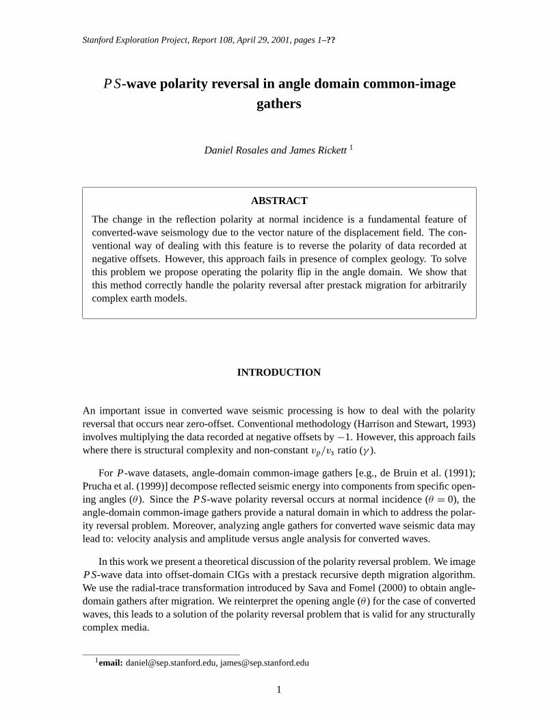
The polarity inversion visible at zero-offset in converted wave data (PS) is an intrinsic prop-erty of the shear wave displacement (Danbom and Domenico, 1988). In a constant velocitymedium, the vector displacement field produces opposite movements in the two geophones ateither side of the source (Figure 1). This leads to the polarity flip in the seismic gather.

Figure 1: Polarity inversion in con-verted waves seismic data.+g and-g correspond to positive and nega-tive polarity in a common shot gather.Modified from Tatham and McCor-mack (1991).daniel2-pflip [NR]

PS

S

P

s

+g

−g

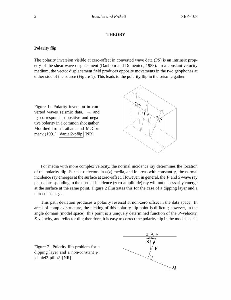
For media with more complex velocity, the normal incidence ray determines the locationof the polarity flip. For flat reflectors inv(z) media, and in areas with constantγ , the normalincidence ray emerges at the surface at zero-offset. However, in general, theP andS-wave raypaths corresponding to the normal-incidence (zero-amplitude) ray will not necessarily emergeat the surface at the same point. Figure 2 illustrates this for the case of a dipping layer and anon-constantγ .

This path deviation produces a polarity reversal at non-zero offset in the data space. Inareas of complex structure, the picking of this polarity flip point is difficult; however, in theangle domain (model space), this point is a uniquely determined function of theP-velocity,S-velocity, and reflector dip; therefore, it is easy to correct the polarity flip in the model space.

Figure 2: Polarity flip problem for adipping layer and a non-constantγ .daniel2-pflip2 [NR]

P

α

S

sg0

h

SEP–108 Converted waves 3

Converted-wave migration by depth extrapolation

Recursive migration methods based on wavefield extrapolation have the advantage over Kirch-hoff methods in that they accurately handle the finite-frequency effects of wave-propagation.For example, rough velocity models and triplicating wavefronts that can cause problems forKirchhoff migrations present no difficulties for recursive methods. Biondi (2000) demon-strated these advantages for a complex 3-DP-wave dataset.

For the examples in this paper, we migrated the prestack data with a shot-profile migrationalgorithm, imaging the cross-correlation of upgoing and downgoing wavefields at zero-time(Claerbout, 1971); however, the methodology is also applicable for “survey-sinking” shot-geophone algorithms based on the double square root equation (Claerbout, 1985).

Migrating converted waves with conventional wavefield extrapolation algorithms simplyinvolves extrapolating downgoing waves with theP-wave velocity field, and upgoing waveswith the S-wave velocity field. The difficulty comes in the interpretation of common-imagegathers in terms of incidence angle at the reflector.

Angle domain common image gathers

Both de Bruin et al. (1991) and Prucha et al. (1999) obtainP-wave angle-domain common-image gathers by slant-stacking the wavefields during migration, before invoking the imagingcondition. Their methodologies suit shot-profile and shot-geophone algorithms, respectively.However, we follow an alternative approach advocated by Sava and Fomel (2000).

Fomel (1996) presented the following partial differential equation describing an imagesurface in depth-midpoint-offset space:

tanθ = −∂z

∂h

∣∣∣∣t ,x

, (1)

whereθ is theP-wave opening or incidence angle.

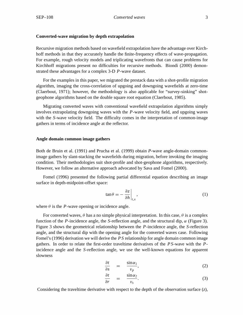
For converted waves,θ has a no simple physical interpretation. In this case,θ is a complexfunction of theP-incidence angle, theS-reflection angle, and the structural dip,α (Figure 3).Figure 3 shows the geometrical relationship between theP-incidence angle, theS-reflectionangle, and the structural dip with the opening angle for the converted waves case. FollowingFomel’s (1996) derivation we will derive thePSrelationship for angle domain common imagegathers. In order to relate the first-order traveltime derivatives of thePS-wave with theP-incidence angle and theS-reflection angle, we use the well-known equations for apparentslowness

∂t

∂s=

sinα1

vp, (2)

∂t

∂r=

sinα2

vs. (3)

Considering the traveltime derivative with respect to the depth of the observation surface (z),

4 Rosales and Rickett SEP–108

Figure 3: Reflection rays for aPS-data in a constant velocity medium(Adapted from Fomel (1996)).daniel2-sergey[NR]

βp

βs

S

s g

α2αα1

α

P

the contributions of the two branches of the reflected ray add together to form

−∂t

∂z=

cosα1

vp+

cosα2

vs. (4)

Introducing midpointx =s+r

2 and half-offseth =r −s

2 coordinates, and relatingα1 andα2 withthe P-incidence angle (βp), theS-reflection angle (βs), and the structural dip (α)

α1 = α −βp,

α2 = α +βs;

and using the chain rule:

∂t

∂x=

∂t

∂s+

∂t

∂r,

∂t

∂h=

∂t

∂r−

∂t

∂s.

We can transform relations (2), (3), and (4) to:

∂t

∂x=

sin(α −βp)

vp+

sin(α +βs)

vs, (5)

∂t

∂h=

sin(α +βs)

vs−

sin(α −βp)

vp, (6)

−∂t

∂z=

cos(α −βp)

vp+

cos(α +βs)

vs. (7)

Dividing (6) by (7) and using elementary trigonometric equalities, we obtain:

−∂z

∂h=

vp sinα cosβs +vp sinβscosα −vssinα cosβp +vssinβp cosα

vp cosα cosβs −vp sinα sinβs +vscosα cosβp +vssinα sinβp= tanθ (8)

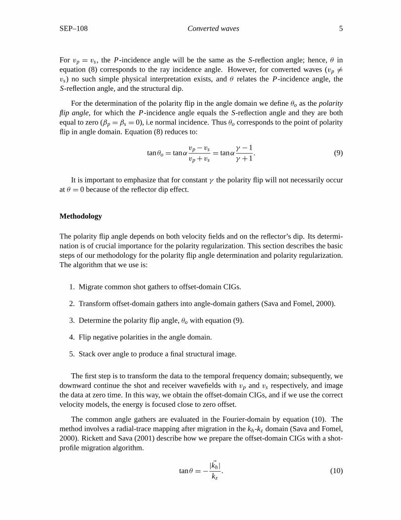
SEP–108 Converted waves 5

For vp = vs, the P-incidence angle will be the same as theS-reflection angle; hence,θ inequation (8) corresponds to the ray incidence angle. However, for converted waves (vp 6=

vs) no such simple physical interpretation exists, andθ relates theP-incidence angle, theS-reflection angle, and the structural dip.

For the determination of the polarity flip in the angle domain we defineθo as thepolarityflip angle, for which theP-incidence angle equals theS-reflection angle and they are bothequal to zero (βp = βs = 0), i.e normal incidence. Thusθo corresponds to the point of polarityflip in angle domain. Equation (8) reduces to:

tanθo = tanαvp −vs

vp +vs= tanα

γ −1

γ +1. (9)

It is important to emphasize that for constantγ the polarity flip will not necessarily occurat θ = 0 because of the reflector dip effect.

Methodology

The polarity flip angle depends on both velocity fields and on the reflector’s dip. Its determi-nation is of crucial importance for the polarity regularization. This section describes the basicsteps of our methodology for the polarity flip angle determination and polarity regularization.The algorithm that we use is:

1. Migrate common shot gathers to offset-domain CIGs.

2. Transform offset-domain gathers into angle-domain gathers (Sava and Fomel, 2000).

3. Determine the polarity flip angle,θo with equation (9).

4. Flip negative polarities in the angle domain.

5. Stack over angle to produce a final structural image.

The first step is to transform the data to the temporal frequency domain; subsequently, wedownward continue the shot and receiver wavefields withvp andvs respectively, and imagethe data at zero time. In this way, we obtain the offset-domain CIGs, and if we use the correctvelocity models, the energy is focused close to zero offset.

The common angle gathers are evaluated in the Fourier-domain by equation (10). Themethod involves a radial-trace mapping after migration in thekh-kz domain (Sava and Fomel,2000). Rickett and Sava (2001) describe how we prepare the offset-domain CIGs with a shot-profile migration algorithm.

tanθ = −| Ekh|

kz. (10)

6 Rosales and Rickett SEP–108

To determine the structural dip, we apply plane-wave destructors (Fomel, 2000), whichcharacterize the seismic images as a superposition of local plane waves. With the dip field andthe two migration velocity models, we calculate the polarity flip angle using equation (9). Flipthe polarity is an easy process after we have the polarity flip angle: we just apply a mask tothe common angle gathers that follows the polarity flip angles and multiply the data by−1.

NUMERICAL EXAMPLES

To test the methodology we created a realistic synthetic example. The model consists of fourreflectors, dipping at angles of 15◦, 0◦, −30◦, −45◦, embedded in simple linearv(z) velocities.

The velocity gradients were chosen in order to simulate a typical near seafloor velocityprofile: theP-velocity model consists of an initial velocity of 1700 m/s and a gradient of 0.15s−1. On the other hand, theS-velocity model has an initial velocity of 300 m/s and a gradientof 0.35 s−1.

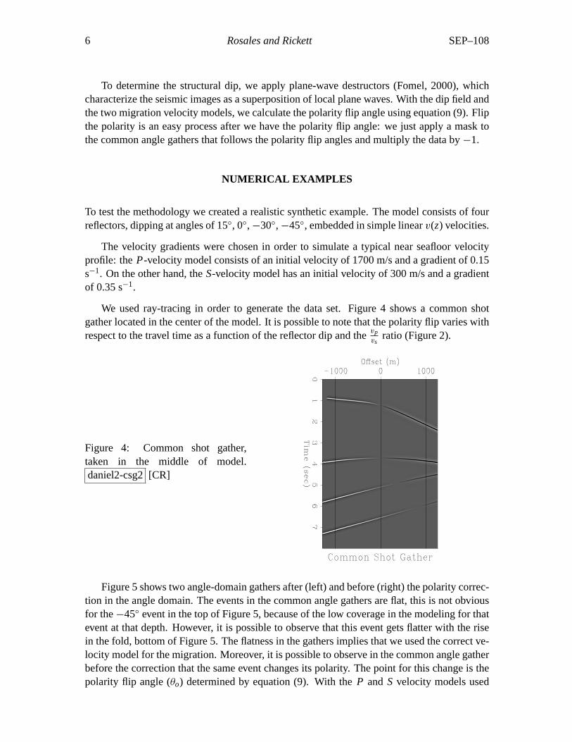
We used ray-tracing in order to generate the data set. Figure 4 shows a common shotgather located in the center of the model. It is possible to note that the polarity flip varies withrespect to the travel time as a function of the reflector dip and thevp

vsratio (Figure 2).

Figure 4: Common shot gather,taken in the middle of model.daniel2-csg2[CR]

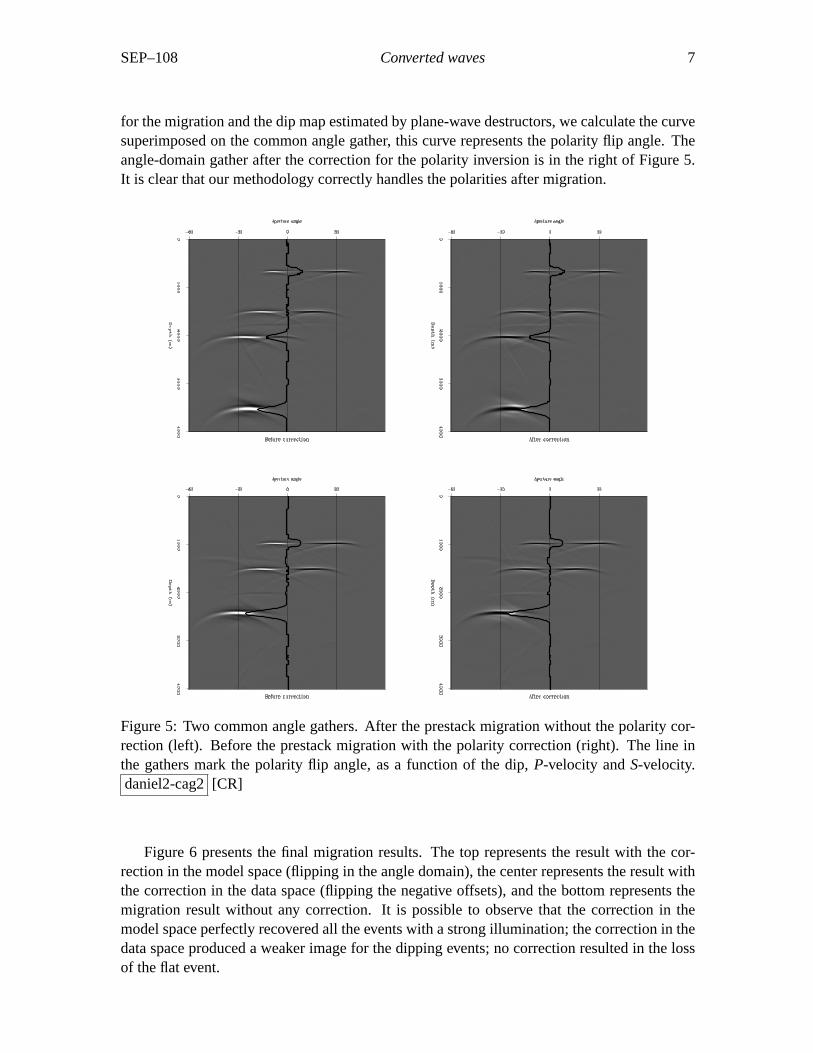
Figure 5 shows two angle-domain gathers after (left) and before (right) the polarity correc-tion in the angle domain. The events in the common angle gathers are flat, this is not obviousfor the−45◦ event in the top of Figure 5, because of the low coverage in the modeling for thatevent at that depth. However, it is possible to observe that this event gets flatter with the risein the fold, bottom of Figure 5. The flatness in the gathers implies that we used the correct ve-locity model for the migration. Moreover, it is possible to observe in the common angle gatherbefore the correction that the same event changes its polarity. The point for this change is thepolarity flip angle (θo) determined by equation (9). With theP and S velocity models used

SEP–108 Converted waves 7

for the migration and the dip map estimated by plane-wave destructors, we calculate the curvesuperimposed on the common angle gather, this curve represents the polarity flip angle. Theangle-domain gather after the correction for the polarity inversion is in the right of Figure 5.It is clear that our methodology correctly handles the polarities after migration.

Figure 5: Two common angle gathers. After the prestack migration without the polarity cor-rection (left). Before the prestack migration with the polarity correction (right). The line inthe gathers mark the polarity flip angle, as a function of the dip,P-velocity andS-velocity.daniel2-cag2[CR]

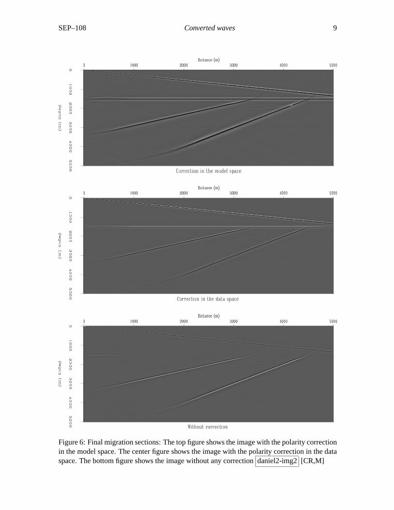
Figure 6 presents the final migration results. The top represents the result with the cor-rection in the model space (flipping in the angle domain), the center represents the result withthe correction in the data space (flipping the negative offsets), and the bottom represents themigration result without any correction. It is possible to observe that the correction in themodel space perfectly recovered all the events with a strong illumination; the correction in thedata space produced a weaker image for the dipping events; no correction resulted in the lossof the flat event.

8 Rosales and Rickett SEP–108

CONCLUSIONS

We presented a series of important concepts in non-conventionalPS-seismic processing foran important problem in converted wave seismic processing: the polarity flip.

We used frequency domain common shot migration in order to obtain an image of thesubsurface with converted wave data. The shot-profile migration algorithm enables the use oftwo different velocity models, one for theP-wave path and the other for theS-wave path ofthe data; therefore, we do not have to introduce a mixedPS-velocity model.

We introduce common angle gather for converted waves. In this domain the normal in-cidence reflection is determined by the polarity flip angle, this polarity flip angle helps toregularize the polarities in the angle domain; we demonstrated this fact with a syntheticPSdata set.

The introduction of common angle gather in converted waves seismic processing andimaging brings a series of opportunities for buildingS-velocity models, and analysis of am-plitude versus angle for converted waves; therefore, the opportunity to extract as much infor-mation as possible fromPSseismic data.

REFERENCES

Biondi, B., 2000, 3-D wave-equation prestack imaging under salt: 70th Ann. Internat. Mtg.,Soc. Expl. Geophys., Expanded Abstracts, 906–909.

Claerbout, J. F., 1971, Toward a unified theory of reflector mapping: Geophysics,36, no. 3,467–481.

Claerbout, J. F., 1985, Imaging the earth’s interior: Blackwell Scientific Publications.

Danbom, S. H., and Domenico, S. N., 1988, Shear-wave exploration: Society of ExplorationGeophysicists.

de Bruin, C. G. M., Wapenaar, C. P. A., and Berkhout, A. J., 1991, Angle-dependent reflectiv-ity by means of prestack migration: Geophysics,55, no. 9, 1223–1234.

Fomel, S., 1996, Migration and velocity analysis by velocity continuation: SEP–92, 159–188.

Fomel, S., 2000, Applications of plane-wave destructor filters: SEP–105, 1–26.

Harrison, M. P., and Stewart, R. R., 1993, Poststack migration of P-SV seismic data: Geo-physics,58, no. 8, 1127–1135.

Prucha, M., Biondi, B., and Symes, W., 1999, Angle-domain common image gathers by wave-equation migration: 69th Annual Internat. Mtg., Society Of Exploration Geophysicists, Ex-panded Abstracts, 824–827.

SEP–108 Converted waves 9

Figure 6: Final migration sections: The top figure shows the image with the polarity correctionin the model space. The center figure shows the image with the polarity correction in the dataspace. The bottom figure shows the image without any correctiondaniel2-img2[CR,M]

10 Rosales and Rickett SEP–108

Rickett, J., and Sava, P., 2001, Offset and angle domain common image gathers for shot-profilemigration: 71st Annual Internat. Mtg., Society Of Exploration Geophysicists, submitted.

Sava, P., and Fomel, S., 2000, Migration angle-gathers by Fourier Transform: GeophysicalProspecting, submitted.

Tatham, R. H., and McCormack, M. D., 1991, Multicomponent seismology in petroleum ex-ploration: Society of Exploration Geophysicists.