Ann Oper ResDOI 10.1007/s10479-015-1855-z

OSGA: genetic-based open-shop schedulingwith consideration of machine maintenancein small and medium enterprises

Shahaboddin Shamshirband1 · Mohammad Shojafar2 ·A. A. Rahmani Hosseinabadi3 · Maryam Kardgar3 ·M. H. N. Md. Nasir4 · Rodina Ahmad4

© Springer Science+Business Media New York 2015

Abstract The problem of open-shop scheduling includes a set of activities which mustbe performed on a limited set of machines. The goal of scheduling in open-shop is thepresentation of a scheduled program for performance of the whole operation, so that theending performance time of all job operations will be minimised. The open-shop schedulingproblem can be solved in polynomial time when all nonzero processing times are equal,becoming equivalent to edge coloring that has the jobs and workstations as its vertices and thathas an edge for every job-workstation pair with a nonzero processing time. For three or moreworkstations, or three or more jobs, with varying processing times, open-shop scheduling isNP-hard. Different algorithms have been presented for open-shop scheduling so far. However,most of these algorithms have not considered the machine maintenance problem. Whilst inproduction level, each machine needs maintenance, and this directly influences the assurancereliability of the system. In this paper, a new genetic-based algorithm to solve the open-shopscheduling problem, namely OSGA, is developed. OSGA considers machine maintenance. Toconfirm the performance of OSGA, it is compared with DGA, SAGA and TSGA algorithms.It is observed that OSGA performs quite well in terms of solution quality and efficiency insmall and medium enterprises (SMEs). The results support the efficiency of the proposedmethod for solving the open-shop scheduling problem, particularly considering machinemaintenance especially in SMEs’.

B Shahaboddin Shamshirbandshamshirband@um.edu.my

Mohammad Shojafarmohammad.shojafar@uniroma1.it

1 Department of Computer System and Technology, Faculty of Computer Science and InformationTechnology, University of Malaya, 50603 Kuala Lumpur, Malaysia

2 Department of Information Engineering Electronics and Telecommunications (DIET),Sapienza University of Rome, Via Eudossiana 18, 00184 Rome, Italy

3 Young Research Club, Behshahr Branch, Islamic Azad University, Behshahr, Iran

4 Department of Software Engineering, Faculty of Computer Science and Information Technology,University of Malaya (UM), 50603 Kuala Lumpur, Malaysia

123

Ann Oper Res

Keywords Timing · Open-shop · Scheduling · Genetic Algorithm

1 Introduction

Scheduling is one of the unavoidable problems in being effective in industrial and economicactivities. Among the most important scheduling problems is open-shop scheduling, whichis widely used in the world of industry. Car repairs, control of central quality, attributionof classes, scheduling inspection and satellite signalling are some of instances discussed byKubiak et al. (1991), Liu and Bulfin (1987) and Prins (1994).

The input to the open-shop scheduling problem consists of a set of n jobs, another set ofm workstations, and a two-dimensional table of the amount of time each job should spendat each workstation (possibly zero). Each job may be processed only at one workstation at atime, and each workstation can process only one job at a time. The aim of scheduling open-shop is to present a scheduled program for assigning a time for each job to be processed byeach workstation, so that no two jobs are assigned to the same workstation at the same time,no job is assigned to two workstations at the same time, and every job is assigned to eachworkstation for the desired amount of time. The open-shop scheduling problem has a verybig solving span but is more complicated in comparison to the job-shop, flow-shop and theflexible manufacturing system (FMS). The open-shop scheduling problem is part of NP-hardproblems and has attracted the concern of many researchers.

Different algorithms have been presented to solve the open-shop problem. Dorndorf et al.(2001) used bound branch and innovative algorithms based on adaptive algorithms and adhe-sive operation. Brasel et al. (1993) offered some algorithms based on heuristic algorithms,adaptation and integration of operations, with the aim of minimising the schedule length.Their computational results show that for large problems, their proposed algorithm yieldsexcellent results.

Gonzalez and Sahni (1976) presented an algorithm to solve the O2llCmax problem witha complexity of O(n) for two machines which can be solved in a finish time schedule for nmachines in a Polynomial time. In Pinedo (1995), presented another simple law on distrib-ution called Longest Alternate Processing Time (LAPT), which solves the problem for twomachines in multi-nominal time. He also showed that for M ≥ 3, the open-shop schedulingproblem NP is complete. Brucker et al. (1997) developed a branch and bound method forthe open-shop problem based on the disjunctive graph formulation. They implemented sixbranch and bound algorithms, with different heuristic algorithms for the smaller instances.All versions of their algorithm find the optimal solutions. For the small instances, only onealgorithm terminates within the given time limit, and for hard instances their proposed methodoutperforms a tabu search method. Alcaide et al. (1997) presented a tabu search algorithm tominimise the makespan of the scheduling problem in the open-shop problem by using simplelist scheduling algorithms. They tested their algorithm on random instances. In Yadollahiand Rahmani (2009), proposed a mimetic algorithm for distributed FMS scheduling by con-sidering the maintenance problem. The objective of this algorithm was a tradeoff betweentime and cost. Liaw (2000) presented a hybrid genetic algorithm (HGA), which is a hybrid oftabu search and the basic genetic algorithm, to solve the scheduling problem of open-shop.The proposed algorithm outperforms other existing methods in terms of solution quality. Asgenetic algorithms are the best tools to solve larger open-shops, in Prins (2000) presenteda GA for the scheduling problem of open-shop. His GA is simple, but it has four essentialfeatures of performance, including generation of active schedules, small populations withdistinct makespans, and chromosome reordering to increase the efficacy of the crossover.

123

Ann Oper Res

Taillard (1993) investigated certain problems in the field of scheduling, such as the permu-tations of flow-shop, job-shop and open-shop scheduling problems. None of these considerthe set-up time, nor due dates, nor release dates. They also assume that processing times arefixed. Their objective is to minimise the makespan.

A set of several versions of list scheduling algorithms and bipartite graphs was presentedby Gueret and Prins (1998). The computational results show that these algorithms are betterthan the classical heuristics and can easily solve open-shop instances. In Cheng et al. (1996),conducted a survey on solving classical job-shop problems (JSP) using a genetic algorithm;the survey presents the representation schemes for JSP and various hybrid approaches ofgenetic algorithms. Matta (2009) studied the multiprocessor open-shop (MPOS) problemand developed two original mixed integer programming formulations for the proportionateMPOS, using the genetic algorithm to schedule all jobs with the aim of minimising themakespan. Matta and Elmaghraby (2010) considered a hospital diagnostic testing centrethat schedules hundreds of patients as a multiprocessor open-shop (MPOS) problem anddeveloped a two-phase scheduling method to solve it. Kordon and Rebaine (2010) investigatedthe problem of scheduling a set of n jobs with time delay considerations, and presented twoapproaches to solve it. The first approach included two special patterns for solvable cases andthe second approach included two heuristic algorithms, including an online algorithm and asorting algorithm. The criterion was to minimise the makespan. Some two-phase heuristicalgorithms for the open-shop scheduling problem with movable dedicated machines andwithout time restrictions were presented by Baccarelli et al. (2012), Hosseinabadi et al.(2014a, b), Lina et al. (2008), Pooranian et al. (2011). The aim of these solutions was toreduce the social costs, such as air pollution and traffic congestion. Andresen et al. (2008)developed two algorithms, namely simulated annealing and a genetic algorithm, to minimisethe completion time. They also compared their algorithms to each other; the results show thatthe genetic algorithm is superior to simulated annealing. Liaw (2000) combined the propertiesof the genetic algorithm and tabu search and proposed a hybrid algorithm, namely HGA, tosolve the open-shop scheduling problem, with the aim of minimising the makespan. Thesimulation results show that this algorithm can produce high-quality solutions. Hybrid antcolony optimisation (HACO) Panahi and Moghaddam (2011), which is based on simulatedannealing and ant colony optimisation, was developed for minimising the makespan andtotal tardiness in the open-shop scheduling problem. Sha and Hsu (2008), by modifyingthe particle position representation, presented a new particle swarm optimisation (PSO) forscheduling in open-shop and reducing the makespan. Low and Yeh proposed a genetic-basedscheduling algorithm Baccarelli et al. (2012) and Low and Yeh (2009) for minimising jobtardiness in open-shop. They took into account some restrictions, such as setup time andremoval time. Yu et al. (2011) presented improved approximation algorithms for routingopen-shop and flow shop scheduling. The aim of these algorithms was to minimise themakespan.

In general, most of the presented algorithms for solving the open-shop problem do nottake the problem of machine maintenance into account. While in production level, eachmachine needs maintenance, and this directly influences the availability of machines, theproduction rate and the usage rate. So, neglecting the maintenance problem reduces theassurance capability of machines and systems.

This paper presents a new GA to solve the scheduling problem of open-shop. Its aim is toreduce the ending time of all jobs and it has the additional advantage that the proposed algo-rithm considers the problem of machine maintenance. The input of the proposed algorithmis jobs and operations, and the output is reducing the finish time of the jobs.

123

Ann Oper Res

The remainder of the paper is set out as follows. In Sect. 2, the problem is described;Sect. 3 explains the proposed algorithm; Sect. 4 gives the computational results; and Sect. 5presents the conclusion.

2 Problem description

In open-shop production there is a set of n jobs, and each job must be performed by mmachine. In other words, each job consists of a set of m operations and each operation shouldbe performed by previously defined machines in a known time span (i.e., according to aspecific considered deadline). The aim of scheduling open-shop production is to reduce theending time of the performance of all operations’ makespan. The scheduling problem ofopen-shop is similar to the job-shop problem; the only difference is that there is no priorityfor the performance of each job. In other words, the jobs can be performed in any order.

Based on the mentioned problem, the following issues are notable:

N: number of jobsM: number of machinesT: time indexi: ith jobj: jth jobmi: number of jobs must be performed by ith machinenj: number of operations of jth jobTi: finish time of ith jobTEij: finish time of ith operation of jth jobXijtm: if the ith operation of jth job is on the ith machine on time T, the Xijtm is equalto 1; otherwise it is 0.

The open-shop scheduling problem has the following restrictions:

1. Every operation must be performed on its own machine∑

Tm

Xi jtm ≥ 1 {i = 1, 2, . . . , m; j = 1, 2, 4, . . . , n; t = 1, 2, 3, . . . , T } (1)

2. Each operation must be performed on one machine and within a specific time.∑

i j

Xi j tm ≤ 1 {i = 1, 2, . . . , m; j = 1, 2, 4, . . . , n; t = 1, 2, 3, . . . , T } (2)

3. In each time, only one operation from one job can be performed.

M∑

1

Xi jtm ≥ 1 {i = 1, 2, . . . , m; j = 1, 2, 4, . . . , n; t = 1, 2, 3, . . . , T } (3)

4. Preemption is not allowed. This means that when an operation is being performed on amachine, it must be performed until it is finished.

T Ei j − T Si j =M∑

1

Xi jtm (4)

5. There is no priority for operation selection, and the operations can be performed indifferent orders.

123

Ann Oper Res

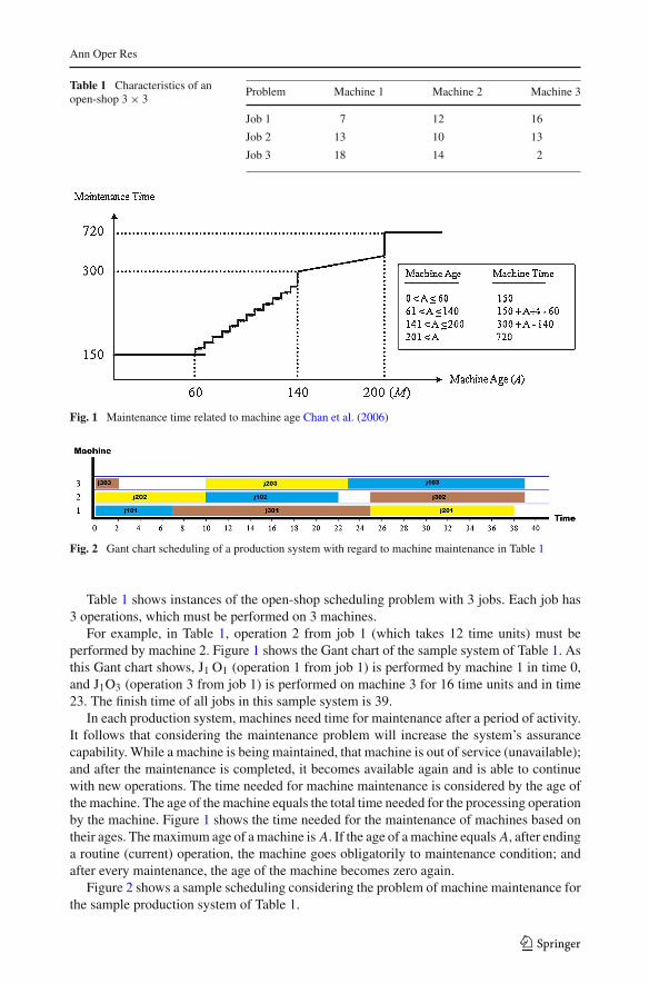
Table 1 Characteristics of anopen-shop 3 × 3

Problem Machine 1 Machine 2 Machine 3

Job 1 7 12 16

Job 2 13 10 13

Job 3 18 14 2

Fig. 1 Maintenance time related to machine age Chan et al. (2006)

Fig. 2 Gant chart scheduling of a production system with regard to machine maintenance in Table 1

Table 1 shows instances of the open-shop scheduling problem with 3 jobs. Each job has3 operations, which must be performed on 3 machines.

For example, in Table 1, operation 2 from job 1 (which takes 12 time units) must beperformed by machine 2. Figure 1 shows the Gant chart of the sample system of Table 1. Asthis Gant chart shows, J1 O1 (operation 1 from job 1) is performed by machine 1 in time 0,and J1O3 (operation 3 from job 1) is performed on machine 3 for 16 time units and in time23. The finish time of all jobs in this sample system is 39.

In each production system, machines need time for maintenance after a period of activity.It follows that considering the maintenance problem will increase the system’s assurancecapability. While a machine is being maintained, that machine is out of service (unavailable);and after the maintenance is completed, it becomes available again and is able to continuewith new operations. The time needed for machine maintenance is considered by the age ofthe machine. The age of the machine equals the total time needed for the processing operationby the machine. Figure 1 shows the time needed for the maintenance of machines based ontheir ages. The maximum age of a machine is A. If the age of a machine equals A, after endinga routine (current) operation, the machine goes obligatorily to maintenance condition; andafter every maintenance, the age of the machine becomes zero again.

Figure 2 shows a sample scheduling considering the problem of machine maintenance forthe sample production system of Table 1.

123

Ann Oper Res

3 Proposed algorithm

In this paper, a new genetic-based approach is presented to solve scheduling open productionsystems. The proposed algorithm focuses variety in genetic operations to achieve a bettersearch in solving the problem and to obtain better responses. The complete structure of theproposed algorithm is given below.

3.1 Chromosome display

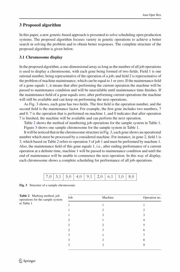
In the proposed algorithm, a one-dimensional array as long as the number of all job operationsis used to display a chromosome, with each gene being formed of two fields. Field 1 is onerational number, being representative of the operation of a job; and field 2 is representative ofthe problem of machine maintenance, which can be equal to 1 or zero. If the maintenance fieldof a gene equals 1, it means that after performing the current operation the machine will bepassed to maintenance condition and will be unavailable until maintenance time finishes. Ifthe maintenance field of a gene equals zero, after performing current operations the machinewill still be available and can keep on performing the next operations.

As Fig. 3 shows, each gene has two fields. The first field is the operation number, and thesecond field is the maintenance factor. For example, the first gene includes two numbers, 7and 0. 7 is the operation that is performed on machine 1, and 0 indicates that after operation7 is finished, the machine will be available and can perform the next operation.

Table 2 shows the method of numbering job operations for the sample system in Table 1.Figure 3 shows one sample chromosome for the sample system in Table 1.It will be noticed that in the chromosome structure in Fig. 3, each gene shows an operational

number which must be processed by a considered machine. For instance, in gene 2, field 1 is3, which based on Table 2 refers to operation 3 of job 1 and must be performed by machine 1.Also, the maintenance field of this gene equals 1, i.e., after ending performance of a currentoperation at a definite time, machine 1 will be passed to maintenance condition and until theend of maintenance will be unable to commence the next operation. In this way of display,each chromosome shows a complete scheduling for performance of all job operations.

7,0 3,1 5,0 4,0 9,1 2,0 6,1 1,0 8,0 Fig. 3 Structure of a sample chromosome

Table 2 Marking method, joboperations for the sample systemin Table 1

Job Machine Operation no.

1 1 1

1 2 2

1 3 3

2 1 4

2 2 5

2 3 6

3 1 7

3 2 8

3 3 9

123

Ann Oper Res

Fig. 4 Crossover operation

3.2 Fitness function

The fitness of chromosomes is calculated based on the time needed to finish all the jobs. Inour algorithm, the fitness function is as in formula 5:

Fitness = Max1 < I ≤ n {Ti} (5)

In this formula, ‘n’ is the number of jobs and Ti is the ending time of job I in scheduling.

3.3 Parent selection

We use the ranking method for selecting the parents. In the ranking method, all chromosomesare arranged according to their fitness, based on the following equation:

(max − Fiti ) + 1Cri ≤ in ≤ n (6)

Cri is the rank of the ith chromosome, ‘max’ is the highest fitness or the worst fitness, andFiti is the fitness of the ith chromosome. The rank of the best chromosome is Max-Fiti + 1(‘max’ is the highest fitness) and the rank of the worst chromosome is equal to 1. Therefore,in this selection method all chromosomes have the chance to be selected.

3.4 Crossover operation

In the OSGA, a random number in the range of 1 to n is first chosen. The genes which existin the range of zero to the random number are transferred from the first parent to the child,and any identical genes are omitted from the second parent. The remaining genes from thesecond parent are inserted in the respective empty blanks of the child. Figure 4 shows asample transfer operation in the proposed algorithm.

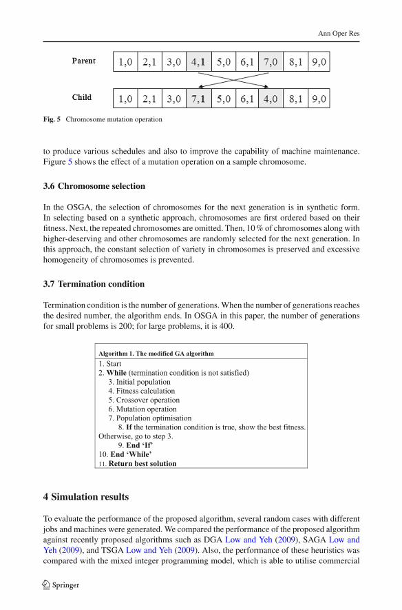
3.5 Mutation operation

In a mutation operation, after choosing a random chromosome of the parent, two genesare chosen randomly and their positions are changed. Then the maintenance field of thesetwo genes is inverted, i.e., if the maintenance field of a gene is 1, it equals zero, and if themaintenance field of the gene is zero, it equals 1. This kind of mutation operation attempts

123

Ann Oper Res

Fig. 5 Chromosome mutation operation

to produce various schedules and also to improve the capability of machine maintenance.Figure 5 shows the effect of a mutation operation on a sample chromosome.

3.6 Chromosome selection

In the OSGA, the selection of chromosomes for the next generation is in synthetic form.In selecting based on a synthetic approach, chromosomes are first ordered based on theirfitness. Next, the repeated chromosomes are omitted. Then, 10 % of chromosomes along withhigher-deserving and other chromosomes are randomly selected for the next generation. Inthis approach, the constant selection of variety in chromosomes is preserved and excessivehomogeneity of chromosomes is prevented.

3.7 Termination condition

Termination condition is the number of generations. When the number of generations reachesthe desired number, the algorithm ends. In OSGA in this paper, the number of generationsfor small problems is 200; for large problems, it is 400.

Algorithm 1. The modified GA algorithm1. Start2. While (termination condition is not satisfied)

3. Initial population4. Fitness calculation5. Crossover operation6. Mutation operation7. Population optimisation

8. If the termination condition is true, show the best fitness. Otherwise, go to step 3.

9. End ‘If’10. End ‘While’11. Return best solution

4 Simulation results

To evaluate the performance of the proposed algorithm, several random cases with differentjobs and machines were generated. We compared the performance of the proposed algorithmagainst recently proposed algorithms such as DGA Low and Yeh (2009), SAGA Low andYeh (2009), and TSGA Low and Yeh (2009). Also, the performance of these heuristics wascompared with the mixed integer programming model, which is able to utilise commercial

123

Ann Oper Res

software such as Lindo or Cplex, or the recently proposed scheduling methods, to generateoptimised solutions.

All of these methods were implemented using the C# programming language and ran on apersonal computer with 2.4GHz Pentium-IV processor and 2GB RAM. Two computationalexperiments are investigated in this section.

4.1 Testing sets of problems

To implement a comparison of the findings from the proposed hybrid heuristics, some testproblems for each manufacturing environment were randomly generated. The details are asfollows:

(1) A manufacturing environment is defined as a set of jobs in a machines scenario in whichthe number of jobs can be (3, 4) or (10, 30, 50), and the number of machines can be(2, 3) or (5, 10, 15).

(2) The time is a certain specific proportion ratio for each operation. It is defined assetup/processing scenario. We consider seven types of time scenarios in this research:10:1:10, 5:1:5, 3:1:3, 1:1:1, 1:3:1, 1:5:1, and 1:10:1. The processing time for each jobis an integer number in (10,100).

4.2 Adaptability verification

To verify the adaptability of the proposed algorithm, we compare it with the three aforemen-tioned methods. The main body of these methods is the genetic algorithm. The differencebetween the methods is in their local optimisations, which are implemented by GA, SA,and TS. The structure of TS and SA with a short memory is the same as in classical forms[(simulated annealing (SA) Laarhoven and Aarts (1987), tabu search (TS) Glover and Laguna(1997)].

The neighbour selection strategy for both TS and SA is an adjacent pair exchange. In thissection the proposed algorithm (OSGA) and DGA, SAGA and TSGA are explained. Theirperformance was evaluated in small problems (job size n=3 or 4; machine size m=2 or 3)and then a comparison with the optimum solution was performed Low and Yeh (2009).

In this paper, four test problems (denoted by k with {1, 2, 3, 4}) were generated for eachmanufacturing scenario, in which each test problem ran 10 times. The results are shown inTable 3. They indicate that in the first three scenarios—3 × 2, 3 × 3, 4 × 2—and in eachrun of test problems, the proposed algorithm and the compared algorithms could obtain anoptimum solution. In scenario 4 × 3, for 50 running hours the proposed algorithm (OSGA)could obtain the best schedule (solution). Also, the computation cost of these four algorithmsis less than 0.4 s.

4.3 Solution quality and efficiency of various heuristics

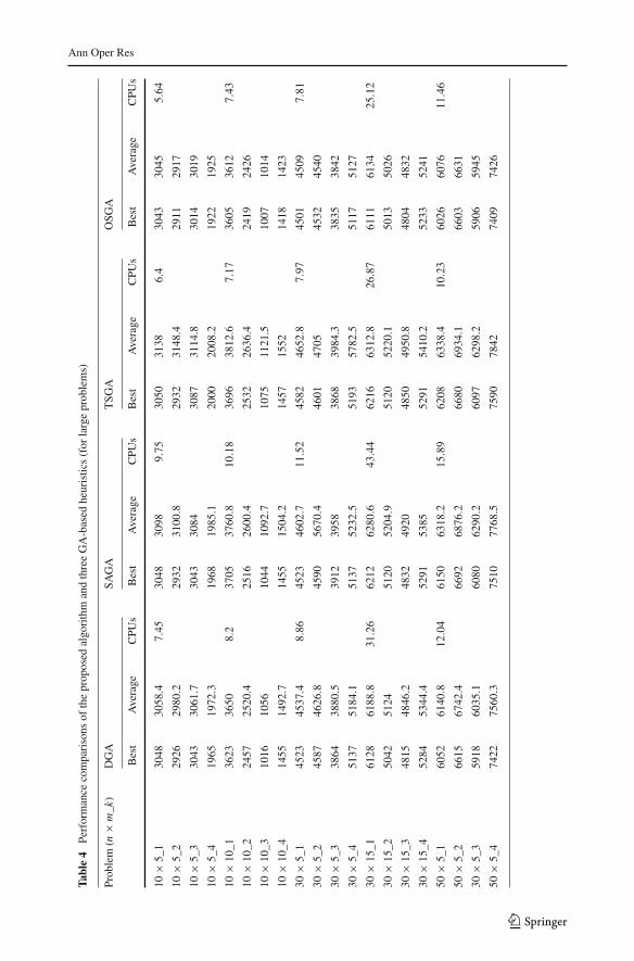
To demonstrate the performance of the proposed algorithm (OSGA), we compared it withthree hybrid algorithms: DGA, SAGA, and TSGA Low and Yeh (2009). We evaluated theperformance of these algorithms in medium and large test problems suitable for industry(job size n = 10, 30, or 50; machine size m = 5, 10, or 15) in terms of solution qualityand efficiency. Four random test problems were generated for each manufacturing scenarioand each test problem ran 10 times. As mentioned in the previous section, the structure and

123

Ann Oper Res

Tabl

e3

Perf

orm

ance

com

pari

sons

ofth

epr

opos

edal

gori

thm

and

thre

eG

A-b

ased

heur

istic

s(f

orsm

allp

robl

ems)

Prob

lem

(n×

m_k

)O

ptim

umso

lutio

nsD

GA

SAG

AT

SGA

OSG

A

Bes

tA

vera

geB

est

Ave

rage

Bes

tA

vera

geB

est

Ave

rage

3×

2_1

177

177

177

177

177

177

177

177

177

3×

2_2

109

109

109

109

109

109

109

109

109

3×

2_3

224

224

224

224

224

224

224

224

224

3×

2_4

241

241

241

241

241

241

241

241

241

3×

3_1

173

173

173

173

173

173

173

173

173

3×

3_2

193

193

193

193

193

193

193

193

193

3×

3_3

212

212

212

212

212

212

212

212

212

3×

3_4

255

255

255

255

255

255

255

255

255

4×

2_1

352

352

352

352

352

352

352

352

352

4×

2_2

393

393

393

393

393

393

393

393

393

4×

2_3

408

408

408

408

408

408

408

408

408

4×

2_4

556

556

556

556

556

556

556

556

556

4×

3_1

–40

240

4.2

402

405.

040

241

0.3

399

401

4×

3_2

–48

748

748

949

2.2

487

493.

148

348

4

4×

3_3

–60

560

5.6

605

607.

060

560

7.4

601

601

4×

3_4

–38

838

8.6

388

389.

238

838

8.8

382

382

“–”

indi

cate

sth

atth

eop

timum

solu

tions

coul

dno

tbe

obta

ined

byth

eex

tend

edL

indo

with

in50

runn

ing

hour

s

123

Ann Oper Res

Tabl

e4

Perf

orm

ance

com

pari

sons

ofth

epr

opos

edal

gori

thm

and

thre

eG

A-b

ased

heur

istic

s(f

orla

rge

prob

lem

s)

Prob

lem

(n×

m_k

)D

GA

SAG

AT

SGA

OSG

A

Bes

tA

vera

geC

PUs

Bes

tA

vera

geC

PUs

Bes

tA

vera

geC

PUs

Bes

tA

vera

geC

PUs

10×

5_1

3048

3058

.47.

4530

4830

989.

7530

5031

386.

430

4330

455.

64

10×

5_2

2926

2980

.229

3231

00.8

2932

3148

.429

1129

17

10×

5_3

3043

3061

.730

4330

8430

8731

14.8

3014

3019

10×

5_4

1965

1972

.319

6819

85.1

2000

2008

.219

2219

25

10×

10_1

3623

3650

8.2

3705

3760

.810

.18

3696

3812

.67.

1736

0536

127.

43

10×

10_2

2457

2520

.425

1626

00.4

2532

2636

.424

1924

26

10×

10_3

1016

1056

1044

1092

.710

7511

21.5

1007

1014

10×

10_4

1455

1492

.714

5515

04.2

1457

1552

1418

1423

30×

5_1

4523

4537

.48.

8645

2346

02.7

11.5

245

8246

52.8

7.97

4501

4509

7.81

30×

5_2

4587

4626

.845

9056

70.4

4601

4705

4532

4540

30×

5_3

3864

3880

.539

1239

5838

6839

84.3

3835

3842

30×

5_4

5137

5184

.151

3752

32.5

5193

5782

.551

1751

27

30×

15_1

6128

6188

.831

.26

6212

6280

.643

.44

6216

6312

.826

.87

6111

6134

25.1

2

30×

15_2

5042

5124

5120

5204

.951

2052

20.1

5013

5026

30×

15_3

4815

4846

.248

3249

2048

5049

50.8

4804

4832

30×

15_4

5284

5344

.452

9153

8552

9154

10.2

5233

5241

50×

5_1

6052

6140

.812

.04

6150

6318

.215

.89

6208

6338

.410

.23

6026

6076

11.4

6

50×

5_2

6615

6742

.466

9268

76.2

6680

6934

.166

0366

31

30×

5_3

5918

6035

.160

8062

90.2

6097

6298

.259

0659

45

50×

5_4

7422

7560

.375

1077

68.5

7590

7842

7409

7426

123

Ann Oper Res

Tabl

e4

cont

inue

d

Prob

lem

(n×

m_k

)D

GA

SAG

AT

SGA

OSG

A

Bes

tA

vera

geC

PUs

Bes

tA

vera

geC

PUs

Bes

tA

vera

geC

PUs

Bes

tA

vera

geC

PUs

50×

15_1

6485

6604

.245

.28

6540

6876

.559

.62

6605

6950

.538

.84

6419

6453

38.5

2

50×

15_2

8905

9015

.789

9592

50.3

9142

9390

.888

7688

95

50×

15_3

6624

6843

.567

0868

7067

0869

40.3

6604

6638

50×

15_4

7350

7413

.673

9575

22.6

7395

7560

.773

1573

52

10×

5_1

3136

3190

.42

3136

3209

.72.

4431

3832

69.8

1.86

3109

3166

2.26

10×

5_2

3094

3245

.831

5232

86.4

3104

3323

.630

2830

77

10×

5_3

3258

3328

.133

1534

09.1

3250

3423

.732

2332

85

10×

5_4

2183

2241

.622

5023

08.2

2261

2337

.421

4621

93

10×

10_1

3802

3872

.42.

1838

1239

05.5

2.75

3850

4014

.51.

7637

9338

172.

11

10×

10_2

2565

2654

.226

0827

61.2

2652

2906

.925

3125

74

10×

10_3

1173

1305

.712

4213

23.8

1238

1338

.111

2811

63

10×

10_4

1587

1622

.515

8716

45.9

1587

1749

1542

1581

30×

5_1

4694

4765

2.5

4712

4814

.22.

9447

4048

84.2

2.16

4659

4696

2.01

30×

5_2

4776

4852

.347

7248

60.9

4776

4963

.647

3847

64

30×

5_3

4159

4240

.742

9143

36.3

4268

4314

.641

2241

72

30×

5_4

5276

5360

.652

7653

73.8

5348

5511

.352

4952

88

30×

15_1

6312

6455

.89.

4564

0165

13.8

10.2

164

2865

85.8

8.51

6283

6317

8.17

30×

15_2

5248

5475

.253

6455

16.1

5272

5513

.552

1152

36

30×

15_3

5024

5150

5081

5169

.350

7852

20.2

5001

5042

30×

15_4

5420

5544

.755

4256

69.3

5502

5613

.354

0354

41

50×

5_1

6341

6480

.53 .

3463

7264

77.6

4.08

6390

6622

2.57

6319

6327

2.35

123

Ann Oper Res

Tabl

e4

cont

inue

d

Prob

lem

(n×

m_k

)D

GA

SAG

AT

SGA

OSG

A

Bes

tA

vera

geC

PUs

Bes

tA

vera

geC

PUs

Bes

tA

vera

geC

PUs

Bes

tA

vera

geC

PUs

50×

5_2

7175

7270

.472

5675

07.4

7264

7711

.271

3671

65

50×

5_3

6374

6457

6386

6446

.664

0565

01.4

6342

6385

50×

5_4

7809

7915

.879

2080

10.8

7974

8145

.977

9278

24

50×

15_1

6952

7068

.213

.470

4871

34.1

14.6

7120

7195

12.1

269

1569

4611

.96

50×

15_2

9506

9760

.596

0298

08.7

9688

9995

.994

9195

17

50×

15_3

7040

7234

.871

6272

40.5

7184

7302

.370

0770

34

50×

15_4

7665

7740

7782

7981

7796

8148

.176

3176

59

123

Ann Oper Res

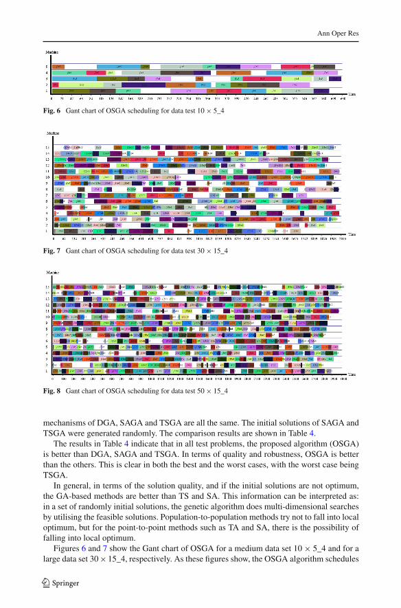
Fig. 6 Gant chart of OSGA scheduling for data test 10 × 5_4

Fig. 7 Gant chart of OSGA scheduling for data test 30 × 15_4

Fig. 8 Gant chart of OSGA scheduling for data test 50 × 15_4

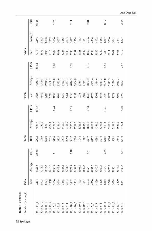
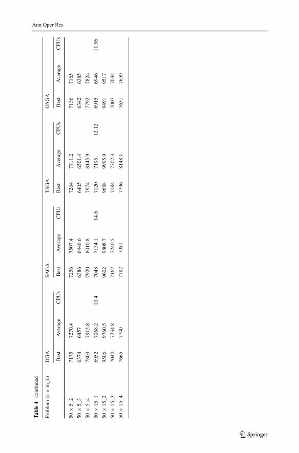
mechanisms of DGA, SAGA and TSGA are all the same. The initial solutions of SAGA andTSGA were generated randomly. The comparison results are shown in Table 4.

The results in Table 4 indicate that in all test problems, the proposed algorithm (OSGA)is better than DGA, SAGA and TSGA. In terms of quality and robustness, OSGA is betterthan the others. This is clear in both the best and the worst cases, with the worst case beingTSGA.

In general, in terms of the solution quality, and if the initial solutions are not optimum,the GA-based methods are better than TS and SA. This information can be interpreted as:in a set of randomly initial solutions, the genetic algorithm does multi-dimensional searchesby utilising the feasible solutions. Population-to-population methods try not to fall into localoptimum, but for the point-to-point methods such as TA and SA, there is the possibility offalling into local optimum.

Figures 6 and 7 show the Gant chart of OSGA for a medium data set 10 × 5_4 and for alarge data set 30 × 15_4, respectively. As these figures show, the OSGA algorithm schedules

123

Ann Oper Res

the jobs even by increasing the size of the problem on corresponding machines well. For thesame problem, we conclude that, by increasing three times jobs numbers and even machinenumbers, makespan is increased three times, but the stopping duration for each machine isdecreased enormously. This means that OSGA is adaptive in large job sizes.

Figure 8 shows the Gant chart of the proposed algorithm (OSGA) for a very large dataset 50 × 15_4. The OSGA algorithm is able to schedule the incoming jobs on machinesproperly with less loss of time. Figure 8, compared with Fig. 7, shows that it is able tomanage makespan even with double times of incoming jobs with fixed machines.

5 Conclusion

In this paper, a new approach called OSGA has been presented for solving the open-shopscheduling problem by using the GA. The proposed algorithm was compared with the DGA,SAGA and TSGA algorithms. One of the properties of the proposed algorithm is that itconsiders the machine-maintenance parameter, so enhancing the assurance capability of theopen-shop system. Here, the proposed algorithm emphasises variety in genetic operations toarrive at better solutions. The experimental results show that, because of the use of transferoperation in the proposed algorithm, proper leap and the operation of synthetic choice disper-sion of chromosomes are constantly preserved; and that the algorithm prevents homogeneityof chromosomes, so arriving at better solutions in a shorter time.

Acknowledgments This work has been partially sponsored by University Malaya Research Grant under thegrant no: RG327-15AFR and Grant (No. RG316-14AFR). We thank the reviewers and associate editor fortheir comments which improved this manuscript

References

Alcaide, D., Sicilia, J., & Vigo, D. (1997). Atabu search algorithmfor the open-shop problem. Top, 5, 283–286.Andresen, M., Brasel, H., Morig, M., Tusch, J., Werner, F., & Willenius, P. (2008). Simulated annealing

and genetic algorithms for minimizing mean flow time in an open shop. Mathematical and ComputerModelling, 48, 1279–1293.

Baccarelli, E., Cordeschi, N., & Patriarca, T. (2012). QoS stochastic traffic engineering for the wireless supportof real-time streaming applications. Computer Networks, 56(1), 287–302.

Baccarelli, E., Cordeschi, N., & Polli, V. (2013). Optimal self-adaptive qos resource management ininterference-affected multicast wireless networks. IEEE/ACM Transactions on Networking (TON), 21(6),1750–1759.

Brasel, H., Tautenhahn, T., & Werner, F. (1993). Constructive heuristic algorithms for the open-shop problem.Computing, 51, 95–110.

Brucker, P., Hurink, J., Jurish, B., & Wostmann, B. (1997). A branch and bound Algorithm for the open-shopproblem. Discrete Applied Mathematics, 76, 43–59.

Chan, F. T. S., Chung, S. H., Chan, L. Y., Finke, G., & Tiwari, M. K. (2006). Solving distributed FMSscheduling problems subject to maintenance: Genetic algorithms approach. Robotics and ComputerIntegrated Manufacturing, 22, 5–6.

Cheng, R., Gen, M., & Tsujimura, Y. (1996). A tutorial survey of job-shop scheduling problems using geneticalgorithms-I. representation. Computers & Industrial Engineering, 30, 983–997.

Dorndorf, U., Pesch, E., & Phan-Huy, T. (2001). Solving the open-shop scheduling problem. Journal ofScheduling, 4, 157–174.

Glover, F., & Laguna, M. (1997). Tabu search. Norwell, MA: Kluwer Academic Publishers.Gonzalez, S., & Sahni, T. (1976). Open-shop scheduling to minimize finish time. Journal of the Assooauon

for Computing Machinery, 23, 665–679.Gueret, C., & Prins, C. (1998). Classical and new heuristics for theshop problem: A computational evaluation.

European Journal of Operational Research, 107, 306–314.

123

Ann Oper Res

Hosseinabadi, A. A. R., Kardgar, M., Shojafar, M., Shamshirband, S., & Abraham, A. (2014a). GELS-GA:Hybrid metaheuristic algorithm for solving multiple travelling salesman problem (pp. 76–81). 14th IEEEISDA.

Hosseinabadi, A. A. R., Siar, H., Shamshirband, S., Shojafar, M., & Nasir M. H. N. M. (2014b). Using thegravitational emulation local search algorithm to solve the multi-objective flexible dynamic job shopscheduling problem in Small and Medium Enterprises. Annals of Operations Research, 1–24.

Kordon, A. M., & Rebaine, D. (2010). The two-machine open-shop problem with unit-time operations andtime delays to minimize the makespan. European Journal of Operational Research, 203, 42–29.

Kubiak, W., Sriskandarajah, C., & Zaras, V. (1991). A note on the complexity of open-shop schedulingproblems. INFOR, 29, 284–294.

Laarhoven, P. J. M., & Aarts, E. H. L. (1987). Simulated annealing: Theory and applications. Norwell, MA:Kluwer Academic Publishers.

Liaw, C. F. (2000). A hybrid genetic algorithm for the open-shop scheduling problem. European Journal ofOperational Research, 124, 28–42.

Lina, H., Leeb, H., & Pan, W. (2008). Heuristics for scheduling in a no-wait open shop withmovable dedicatedmachines. International Journal of Production Economics, 111, 368–377.

Liu, C. Y., & Bulfin, R. L. (1987). Scheduling ordered open-shops. Computers & Operations Research, 14,257–264.

Low, C., & Yeh, Y. (2009). Genetic algorithm-based heuristics for an open shop scheduling problem withsetup, processing, and removal times separated. Robotics and Computer-Integrated Manufacturing, 25,314–322.

Matta, M. E. (2009). A genetic algorithm for the proportionate multiprocessor open shop. Computers &Operations Research, 36, 2601–2618.

Matta, M. E., & Elmaghraby, S. E. (2010). Polynomial time algorithms for two special classes of the propor-tionate multiprocessor open shop. European Journal of Operational Research, 201, 720–728.

Panahi, H., & Moghaddam, R. T. (2011). Solving a multi-objective open shop scheduling problem by a novelhybrid ant colony optimization. Expert Systems with Applications, 38, 2817–2822.

Pinedo, M. (1995). Scheduling: Theory algorithms and systems. Englewood Cliffs, NJ: Prentice-Hall.Pooranian, Z., Harounabadi, A., Shojafar, M., & Hedayat, N. (2011). New hybrid algorithm for task scheduling

in grid computing to decrease missed task. World Academy of Science, Engineering and Technology, 55,924–928.

Prins, C. (1994). An overview of scheduling problems arising in satellite communications. The Journal of theOperational Research Society, 45, 611–623.

Prins, C. (2000). Competitive genetic algorithms for the open-shop scheduling problem. Mathematical Methodsof Operations Research, 52, 389–411.

Sha, D. Y., & Hsu, Ch Y. (2008). A new particle swarm optimization for the open shop scheduling problem.Computers & Operations Research, 35, 324–3261.

Taillard, E. (1993). Benchmarks for basic scheduling problems. European Journal of Operational Research,64, 278–285.

Yadollahi, M., & Rahmani, A. M. (2009). Solving distributed flexible manufacturing systems schedulingproblems subject to maintenance: Memetic algorithms approach. International Conference on Computerand Information Technology, 1, 36–41.

Yu, W., Liu, Zh, Wang, L., & Fan, T. (2011). Routing open shop and flow shop scheduling problems. EuropeanJournal of Operational Research, 213, 24–36.

123