Organization, Learning and Cooperation∗

Jason Barr†and Francesco Saraceno‡

Rutgers University, Newark Working Paper #2004-001

March 2004

Abstract

We model the organization of the firm as a type of artificial neuralnetwork in a duopoly framework. The firm plays a repeated Prisoner’sDilemma type game, but also must learn to map environmental signalsto demand parameters. We study the prospects for cooperation giventhe need for the firm to learn the environment and its rival’s output.We show how a firm’s profit and cooperation rates are affected by itssize, its rival’s size and willingness to cooperate, and environmentalcomplexity.

JEL Classification: C63, C72, D21, D83, L13Keywords: Artificial Neural Networks, Cooperation, Firm Learning

∗An earlier version of this paper was been presented at the 2003 Annual Meeting of theSociety for the Advancement of Behavioral Economics, Lake Tahoe, Nevada, July 29-31.We thank Duncan Foley and seminar participants at the U.S. Naval Academy for theircomments and suggestions. The usual caveats apply.

†Corresponding Author: Department of Economics, Rutgers University, Newark, NJ07102. email: jmbarr@andromeda.rutgers.edu.

‡Observatoire Francais des Conjonctures Economiques, Paris, France. email:francesco.saraceno@sciences-po.fr

1

1 Introduction

Information processing and decision making by firms are not typically doneby one person. Rather decisions are made by a group of people either in acommittee or hierarchical structure. Bounded rationality and/or computa-tional costs preclude the possibility of any one agent collecting, processingand deciding about information relevant to the firm and its profitability.Thus many agents are employed to process this information so that the firmcan make informed decisions. But processing information and decision mak-ing are costly activities. Large firms, for example, employ hundreds eventhousands of ’managers’ who do not produce or sell anything, but ratherprocess information and make decisions (Radner, 1993).Building on previous work (Barr and Saraceno, forthcoming), we model

the firm as a type of artificial neural network (ANN) that must make outputdecisions in a Cournot duopoly framework. The use of ANNs as a model offirm organization allows us to make explicit the nature and cost and benefitsof processing information. Agents within the firm are required to evaluatedata and communicate this evaluation to others who then make final deci-sions. As discussed in Barr and Saraceno (2002; forthcoming), the benefitto the firm of increased resources devoted to information processing (IP) isbetter knowledge of the environment and hence increased returns. But thecosts include the costs of paying agents and the time and costs involved withprocessing and communicating this information.In Barr and Saraceno (forthcoming) we investigated how learning affects

a firm’s ability to produce along the best response function. We show thatANNs competing in a duopoly setting can learn to converge to the Nashequilibrium output, which is changing each period due to changing environ-mental states. Further we show how environmental complexity affects bothorganizational size and profitability. In that setting, firms choose an outputlevel given the observation of the environmental state and, after that, theprice is set, the market clears, and firms then compare their output choicesto the best response they should have played given the output choice of theiropponent.The ANN embodies the knowledge of the firm and implicitly contains

a history of what the rival played in the past. Over time, firms learn toforecast both the effect of changing environmental states on demand and therival’s output; both firms converge to the Nash equilibrium over time. Inthat framework, we did not consider the possibility of collusion in the sense

2

that firms could possibly learn to produce less than Cournot output, thusgaining larger profits.Here, we are interested in studying the prospects for cooperation with

two additional factors as compared to traditional cooperation models (seeAxelrod, 1984): (1) the need for firms to map environmental characteristicsto changing product demand, and (2) many agents within a firm are neededto learn not only the environment but what exactly the rival is signallingabout its output strategy, i.e., whether it will cooperate or defect. We arguethat a firm’s knowledge not only of the environment but also its ability to seewhat its rival is doing will ultimately affect its profitability. If, for example,a firm learns that its rival has a low desire to cooperate, all else equal,it too should change its output to defect most of the time. But if a firmlearns that its rival is willing to cooperate then mutual gains are possible.The difficulty of learning affects a firm’s ability to cooperate, since in highlycomplex environments, firms will have problems distinguishing what part ofthe variation in the market clearing price is coming from the variation in theenvironment versus the variation in the rival’s strategy.

In this paper, we have two neural networks competing in a repeatedduopoly setting. Each period, the firm (network) views an environmentalstate vector (an N -length vector of 00s and 10s) which it uses to estimate twovariables: the intercept parameter of the demand curve, and its rival’s output.The firm uses the estimate of its rival’s output to decide if its rival is goingto defect or cooperate. If the estimate of its rival’s output is greater than theshared-monopoly output (plus some margin), the firm plays the (estimated)Cournot best response, otherwise it plays the (estimated) shared-monopolyresponse. In this sense, both firms are playing a kind of Tit-For-Tat strategy:’I defect if I think you will defect, otherwise I will cooperate.’After each firm chooses an output, it observes the market clearing price,

the rival’s output and the true demand intercept. The firm uses this infor-mation to calculate the error it made in its estimation of the intercept andits rival’s output, and then uses this error to improve its performance in thesubsequent periods. Thus the knowledge of both the environmental charac-teristics and the rival’s past plays lies within the network itself, rather thanany one agent; the network serves as a economical storage device: ’givenwhat I have learned in the past, I now can map environmental informationto a rival’s output and to the demand intercept.’We measure environmental complexity by the number of environmental

3

bits (signals) a firm views each period. Each period a new environmentalvector is randomly chosen with probability of 1/2N , where N is the numberof bits in the vector. This is tantamount to what might be referred to as a’pure generalization’ process.1 In our paper, for N large enough, this has theeffect of having an environment that is changing at each period.In this paper we ask:

• What is the relationship between network size, learning and profitabil-ity given that firms are learning both the environment and their oppo-nent’s behavior?

• How does environmental complexity affect performance, cooperationand profits?

• What is the relationship between a firm’s willingness to be ’nice,’ i.e.,its willingness not to defect given that it estimates its rival will defect,profits and cooperation?

• What is the average firm size and cooperation in equilibrium versusenvironmental complexity?

To anticipate some of our results, we will be drawing three sets of conclu-sions. The first is that environmental complexity and firm dimension interactin a complex way: performance is a function of the not only the difficulty ofthe IP task, but also the rival’s size and willingness to cooperate. Second,we will show that cooperation rates are also affected by environmental com-plexity, firm size, and rival’s behavior. Lastly, we will show how strategicinteraction leads to ’industrial equilibria’ in regards to firm size and coop-eration; and we show how environmental complexity affects these equilibria.

The rest of the paper is as follows. In the next section we briefly reviewthe literature that relates to our paper. The following (section 3) outlines thestandard Cournot model that we work with, which is an extension of the RPD

1In the computer science literature, the type of ANN that we employ—the BackwardPropagation Network—normally ’trains’ on a fixed data set and then is presented new datafor forecasting (Croall and Mason, 1992). After training the network can ’generalize’ inthe sense that it can make forecasts using new, unseen data. Here, the networks train andgeneralize simultaneously.

4

game. Next, section 4 discusses the particular game that the neural networksplay and the characterization of the economic environment. In section 5 wediscuss the workings of the particular ANN that we use. Then sections6 through 8 present the results of our simulation experiments. Finally, insection 9 we present concluding remarks and possible research extensions.

2 Related literature

There is a rich literature on the issue of cooperation and defection in Pris-oner’s Dilemma type games, of which the Cournot game is a variant. In thisgeneral framework, two players must make a decision over two outcomes:whether to cooperate or defect. The result (payoff) of the decision, however,is affected by the rival’s decision. If decisions have to be made repeatedly andthere is little prospect that the game will end in a short time then mutualsustained cooperation is possible, even if there is no direct communication.In the Cournot game, firms can signal their willingness to cooperate overtime by choosing low output over high output. If the other firm ’takes thebait’ by also producing a low output, then their is mutual gain to be had(assuming a sufficiently high discount rate).In terms of the repeated Prisoner’s Dilemma (RPD), a standard game

theoretic result is that of the ’folk theorem,’ which says that if agents arepatient enough, then there are an infinite set of Nash Equilibrium outcomesthat have higher pay-offs than the ’defect every period’ strategy (the so-calledmin-max payoff) (Fudenberg and Tirole, 1991).Recently, models of the RPD have also been concerned with bounded

rationality and the evolution of cooperation. Rubinstein (1986) and Cho(1994) model agents as boundedly rational automata-type machines. Rubin-stein’s machine is a finite automata and Cho’s is a simple perceptron. Thesepapers show the types of equilibria that can arise. If, for example, there is abound placed on level of complexity in Rubinstein’s machine then only a fi-nite number of equilibrium outcomes can be generated. Cho’s machine is ableto ’recover’ the perfect folk theorem using a neural network that maintainsan upper bound on the complexity of equilibrium strategies.While these papers focus on the nature of the machines and the nature of

the equilibria outcomes, other papers focus on the evolution of cooperation(Axelrod, 1997; Miller, 1996; Ho, 1996). For example, Miller demonstrateshow cooperation can evolve overtime if automata machines adapt using a

5

genetic algorithm (Holland, 1975) that allows the strategic environment tochange. Further he studies co-evolution of strategies under imperfect infor-mation. Axelrod (1997) also models the RPD with a genetic algorithm, butfixes the population of possible strategies.Our paper relates to the literature on adaptive machines that play a re-

peated Prisoner’s Dilemma type game but is different in the following ways.First, we are interested in studying an RPD using an agent-based modelof the firm. Our interest is in asking the questions: How are profits andcooperation affected by agent-based learning? And what are the optimalnumber of agents needed to learn both the external economic environmentand the rival’s output decision over time? For simplicity we hold the firms’strategies constant (as a type of Tit-for-Tat strategy) and focus on the rela-tionship between firm complexity (network size), environmental complexity(the quantity of information), profitability and cooperation. Thus our objec-tive is to focus not on the evolution of strategies or the types of equilibriaoutcomes but rather the learning process that firms need to do in order toimprove performance and profits.In addition to RPD games, cooperation in Cournot models have been

widely discussed (see Tirole (1988) for a review of these models). Similarto the RPD, collusion is possible if firms are sufficiently patient and thethreat of punishment exists (Verboven, 1997). Cyret and DeGroot (1973)show cooperation is possible if firms maximize joint profits; further they cancome to cooperate over time by a process of Bayesian learning. Vriend (2000)presents an adaptive model of a Cournot game, where agents evolve accordingto a genetic algorithm. He shows how equilibrium market outcomes can bedifferent depending if agents perform individual rather than social learning.Our model is similar to these papers in the sense that firms are adaptive, butunlike these models, firms’s output decisions evolve based on not only therival’s behavior but also the nature of the environment and on the inherent’niceness’ of firms themselves.Our work also fits within the literature on agent-based models of the firm

(Radner, 1993; DeCanio and Watkins, 1998; Carley, 1996). These models,borrowing heavily from computer science, represent the firm as a network ofinformation processing agents (nodes). In general these papers study whichtypes of networks minimize the costs of processing and communicating in-formation. Our model is also agent-based in the sense that we assume thatoutput decisions by the firm are made by a network of information process-ing agents. However, our work is different in two respects: in general, and

6

unlike other agent-based models, we directly model the relationship betweenthe external environmental variables, firm learning and performance; sec-ondly, we explicitly provide an agent-based model of Cournot competitionand cooperation, which to our knowledge has not been done before.Our agent-based approach models the firm as a type of artificial neu-

ral network, with the nodes representing managers. ANNs are common incomputer science and psychology, where they have been used for patternrecognition and modeling of the brain (Croall and Mason, 1992; Skapura,1996). In economics, neural networks have been employed less frequently.One application has been to use ANNs as non-linear estimation equations(Kuan and White, 1992). Because of the stochastic and non-linear nature ofANNs we employ a simulation-based approach to studying the relationshipbetween firm performance, competition and size.

3 The duopoly framework

This section will give a textbook summary of standard Cournot theory in astatic and repeated framework. Then, in the next section we will introduceuncertainty and show how we model firms as ANNs.Let’s say we have a market with two firms. Each period they face the

demand function

pt = αt − β (q1t + q2t) .

In section 4, α will be a variable, and we will assume that firms must estimateits value from period to period; but for the moment, to review the Cournotgame, we take it as constant and known to the firms. Here and for the restof the paper, we also assume that the slope is constant (and normalized to1). Profits for each firm are

πj = [α− (q1 + q2)] qj − cj, j = 1, 2

where cj is costs, such as the cost of network, and is set to zero for convenienceand without loss of generality.2

2While we do not deny the importance of the cost of carrying a network of a given size,we do not include this cost in the paper for simplicity since the qualitative results wouldnot change.

7

Under standard Cournot assumptions, the best response function is givenby

qbrj =1

2[α− q−j] ,

with a Nash Equilibrium of

qne =α

3, πne

j =1

9α2.

This is a typical prisoner dilemma’s game. If the two firms could coor-dinate their output decisions and act as a monopoly their joint profit fromproduction would be

πm = [α−Q]Q.

Assuming they share production and profits equally, each would have anoptimal output:

qmj =α

4.

Profit would then be

πmj =

1

8α2 > πne

j =1

9α2.

In a single shot game the cooperation outcome is not an equilibrium;3 ifone firm knew that its rival would play half of the monopoly output, thenit could defect by playing its Cournot best response and achieve a higherpayoff:

qdj =1

2[α− qm] =

3

8α

πdj =

9

64α2 > πm

j .

On the other hand, as is well known, if the game is repeated other equi-librium outcomes can emerge.

3Here we define cooperation as splitting the monopoly quantity and defection is eachplaying a best response.

8

3.1 Repeated prisoner dilemmas and the folk theorem

In a repeated framework, firms face the decision each period wether to ’co-operate’ or ’defect.’ Then, whether the horizon is finite or not will yieldcompletely different results. Suppose that the game is repeated an infinitenumber of times, and that firm j0s payoff is given by the discounted sum ofprofits:

Πj =∞Xt=1

δt−1πjt

where δ is the discount rate.4 In this case many other strategies involvingcooperation can constitute an equilibrium, in addition to the ’defect everyperiod’ outcome. Take for example the grim trigger strategy: cooperate untilthe opponent defects; if defection revert to the best response strategy (i.e.,defect) forever. The cooperative outcome will be assured when

πm

1− δ> πd + πne δ

1− δ.

Plugging in the profit values from above, we have for our case δ∗ > 917.

In words, if the discount rate is large enough, future losses will more thancompensate the short run gain from defection, and cooperation will be theoutcome of a grim trigger strategy. But the same could be showed for theso called Tit-For-Tat strategy, which consists of beginning with cooperation,and playing each period what the opponent played in the preceding one.In fact, it can be shown that if the discount rate is high enough, almostany strategy involving cooperation can be an equilibrium strategy. This isin fact what the folk theorem tells us: any feasible expected payoff can besustained in an equilibrium as long as each player can expect an equilibriumpayoff larger than the uncooperative one. In that case, no player will havean incentive to deviate. With a backward induction argument, on the otherhand, it can be shown that cooperation is not sustainable if the game isrepeated a finite number of times.An important extension of the preceding framework that relates to the

present paper is the consideration of the effects of uncertainty on the sustain-ability of cooperative equilibria (Green and Porter, 1984). This is typically

4Notice that δ can either be interpreted as the discount factor of an infinitely repeatedgame, or as the probability that the game is repeated after each round when the gamelength is undefined. analytically the two ’stories’ boil down to the same thing.

9

modelled as price uncertainty; for example, the constant term of a lineardemand function shifts according to a given probability distribution. Theobvious effect of such a feature of the model is that deviations from thecollusive price and profit are not directly attributable to the competitor’sunwillingness to cooperate, but may stem from shifts in the demand func-tion. The punishment scheme designed by a firm to force cooperation has asa consequence to be more complex than in the case of certainty. This typ-ically involves a trade-off, whose outcome depends on the particular modeladopted: if the punishment is too harsh, the firm loses possible advantagesfrom collusion; but if it is too light, then the opponent may be tempted toadopt a noncooperative stance. To sustain cooperation, hence, firms have topunish their opponents only if prices and profits deviate ”too much” fromthe cooperative level. We’ll adopt a similar perspective in what follows, witha crucial difference. We add the possibility that firms can reduce uncertaintyby means of learning; our focus, in fact, is on this learning process, and onhow it affects the willingness to cooperate.

4 Amodel of firm learning in a repeated Cournot

game

4.1 Strategies

In this paper we have each network employ a relatively simple strategy: atype of Tit-for-Tat (TFT). The standard TFT says that a firm should beginby cooperating and then play the same outcome as the rival’s prior move.Given our framework, this strategy allows for the possibility of cooperationonce firms begin to learn the external environment, and learn to separatethe variance in price that is due to environmental change versus their rival’soutput decision.5

In this paper, firms employ a slight variation of the TFT strategy. Since

5TFT, in general, behaves according to the four rules-of-thumb discussed by Axelrod(1984) for strategies that are likely to promote cooperation in a setting where boundedlyrational agents are the players: (1) Be nice: never be the first to defect. (2) Be forgiving :be willing to return to cooperating even if your opponent defects. (3) Be simple: theeasier it is to discover a pattern in a rival’s output the easier it is to learn to cooperate.(4) Don’t be envious: don’t ask how well you are doing compared to your rival, but ratherhow much better you can do, given your rival’s actions.

10

they estimate both the demand parameter and their rival’s output quantityeach period, they have to use this information to decide whether to defect ornot. More specifically the firm chooses an output each period based on thefollowing rule (j = 1, 2, ):

qj =

(12

¡αj − qj−j

¢if³qj−j − αj

4

´> ρj

αj/4 otherwise

), (1)

where qj is firm j 0s output, qj−j is firm j 0s estimate of its rival’s output, andαj is firm j 0s estimate of α. Equation (1) says that if the firm estimates itsrival to be a cheater: qj−j > αj/4 + ρj, i.e., that the rival is expected todeviate from forecast monopoly profit, then it plays the optimal forecastedCournot output; that is, it defects as well.The threshold value ρj ≥ 0 represents the firm’s ’willingness to be nice.’

For relatively small values, e.g., ρj = 0, firm j will play defect relativelymore often; for values ρj ≥ ρ, the firm will be so nice that it will never defect.Notice that in making this decision the firm has two possible sources of error:the first is the environment, and the second is the opponent’s quantity; thisis why it will allow a deviation ρj from the monopoly output before revertingto the noncooperative quantity.

4.2 The economic environment

4.2.1 A shifting demand curve

Here we represent the external environment as a vector of binary digitsx ∈ {0, 1}N . The relationship between the environment and the interceptis given by

α (x) =1

2N

NXk=1

xk2N−k,

xi is the kth element of x. This functional relationship converts a binary digit

vector into its decimal equivalent.6 We can think of this in the followingmanner: the vector x contains signals (information) from the environment,which are arranged in order of increasing importance. α (x) can be thoughtof as a weighted sum of the environmental signals. Each period, the firm

6The value of α is normalized to be between 0 and 1 by dividing by 1/2N.

11

views an environmental vector x and uses this information to estimate thevalue of α (x) .

4.2.2 Environmental change

Each period an environmental vector is randomly chosen with probability1/2N . For example, for N = 10, each vector has a probability of 0.000977of being selected. In our simulations it is very unlikely for an environmentalvector to be viewed by the firm more than once; the learning process high-lights the pattern recognition features of our neural network model of thefirm.

4.2.3 Complexity

To measure the complexity of the information processing problem, we defineenvironmental complexity as the number of bits in the vector, N , which, inthe simulations below, ranges from a minimum of 5 bits to a maximum of60.

4.3 The steps

Here we outline the behavior of the firm each period (time subscripts droppedfor notational convenience):

1. Each firm observes the environmental state vector x.

2. Based on that each firm estimates a value of the intercept parameter,αj. The firm also estimates its rival’s choice of output, qj−j, where q

j−j

is firm j 0s guess of firm −j 0s output.3. Based on the values the firm estimated in step 2, it makes an outputdecision using the TFT-type rule given by equation (1).

4. It then observes the true value of α and q−j, and uses this information

12

to determine its errors using the following rules:7

ε1j = (αj − α)2 (2)

ε2j =

( ¡qj−j − q−j

¢2if¡q−j − αj

4

¢> ρj¡

qj−j − α/4¢2

otherwise

)(3)

Note the contents of equation (3). After the firm observes its rival’soutput it must select a particular error. If it sees that its rival didnot cooperate it therefore yields one error (i.e., the ’did-not-cooperate’one), but if it sees that its rival did cooperate then it uses the othererror. This way the firm uses its rival’s past performance as guide forthe firm’s learning.

5. Based on these errors, the firm updates the weight values in its networkfor improved performance in the next period. This process is outlinedin the next section.

5 The firm as artificial neural network

The neural network is comprised of three ’layers’: the environmental data(i.e., the environmental state vectors), a hidden/managerial layer, and anoutput/decision layer.8 The ’nodes’ in the managerial and decision layersrepresent the information processing behavior of agents. Each agent takesa weighted sum of the information it views and applies a type of squashingfunction to produces an output/signal: a value between zero and one. In themanagerial layer, this output is then passed/communicated to the decisionlayer. Each output node takes a weighted sum of the signals from the man-agerial layer to produce a particular decision: an estimated intercept valueor an estimated rival’s output. A graph of the network is shown in Figure 1.This type of ANN is referred to as a backward propagation network (BPN).

7In Barr and Saraceno (forthcoming) we demonstrate the how profit and error arenegatively related, and that maximizing profit is the same as minimizing the error. Forthe sake of brevity, we do not show a similar result in this paper since the error ruleis relatively more complex, but the same result applies in this case and is confirmed byregression analysis (results not shown).

8See Barr and Saraceon (2002; forthcoming) for more details about using ANNs asmodels of the firm.

13

Figure 1: A graph of a neural network.

More specifically, the environmental data (information) layer is a binaryvector x ∈ X of length N . Each manager (node) in the management (hidden)layer takes a weighted sum of the data from the data layer. That is, the ith

agent in the management layer of firm j calculates

inhij = w

hijx ≡

£wh

1ix1 + . . . + whNixN

¤, i = 1, . . . ,Mj; j = 1, 2.

Thus the set of ’inputs’ to the Mj managers of the management layer is

inhj =

³inh

1j, . . . , inhij, . . . , in

hMj

´=³wh

1jx, ...,whijx, ...,w

hMjjx´.

Each manager then transforms the inputs via a squashing (voting) functionto produce an output, outhij. Here we use one of the most common squash-

ing functions, the sigmoid function: outhij = g(inhij) = 1/

¡1 + exp

¡−inhij

¢¢.

Large negative values are squashed to zero, high positive ones are squashedto one, and values close to zero are ’squashed’ to values close to 0.5.9

The vector of processed outputs from the management layer is

outhj =³outh1j, . . . , out

hij, . . . , out

hMjj

´=³g(inh

1j), ..., g(inhij), ..., g(in

hMjj)´.

9The sigmoid function can represent the votes of managers since the sigmoid is a con-tinous version of the Heaviside function.

14

The inputs to the output layer are weighted sums of all the outputs from thehidden layer:

inoιj = w

oιjout

hj ≡

³wo

1ιjouth1j + ...+ wo

Mj ι jouthMj j

´, ι = 1, 2.

All weights in both layers can take on any real value. Finally, the outputs ofthe network—the estimate of demand intercept αj and q

j−j—are determined by

transforming inoιj via the sigmoid function,

©αj = g

¡ino

1j

¢, qj−j = g

¡ino

2j

¢ª.

We can summarize the behavior of network with two outputs as

αj = g

MjXi=1

woi1jg

¡wh

ijx¢ ,

qj−j = g

MjXi=1

woi2jg

¡wh

ijx¢ .

5.1 The learning algorithm

The above process describes the input-output nature of the neural network.However, the distinguishing feature of the network is its ability to learn.After the market price is set and the market clears, the firms learn the truevalues of the intercept and rival’s output. They then use this informationto help improve their performance in successive periods. They calculate theerror they made and then update the network weights using a gradient decentmethod that changes the weights in the opposite direction of the gradient ofthe error with respect to the weight values. We begin with a completelyuntrained network by selecting random weight values (i.e., we assume thenetwork begins with no prior knowledge of the environment).An environmental state vector is realized and the networks processes it, as

described above, to obtain outputs©αj, q

j−jª. These outputs are compared

to true values to get an error for each one, according to equations (2) and(3). Total error is then calculated:

ξj = ε1j + ε2j

This information is then propagated backwards as the weights are ad-justed according to the learning algorithm, that aims at minimizing the total

15

error, ξj. Define yj =©αj, q

j−j

ªand yj = {α, q−j} . The gradient of ξj with

respect to the output-layer weights is

∂ξj∂wo

iιj

= −2 ¡yιj − g¡ino

ιj

¢¢g0¡ino

ιj

¢outhij,

where i = 1, ...,Mj; ι = 1, 2; j = 1, 2. For the sigmoid function, g0 ¡ino

ιj

¢=

yιj(1− yιj).Similarly, we can find the gradient of the error surface with respect to the

hidden layer weights:

∂ξj∂wh

ikj

= −2g0(inhikj)xk

£¡yιj − g

¡ino

ιj

¢¢g0¡ino

ιj

¢wo

iιj

¤,

where i = 1, ...,Mj; ι = 1, 2; j = 1, 2; k = 1, ..., N.Once the gradients are calculated, the weights are adjusted a small amount

in the opposite (negative) direction of the gradient. We introduce a propor-tionality constant η, the learning-rate parameter, to smooth the updatingprocess. If we define δoιj = .5(yιj − yιj)g

0(inoιj), we have the weight adjust-

ment for the output layer as

woiιj(t+ 1) = wo

iιj(t) + ηδoιjouthij.

Similarly, for the hidden layer,

whijk(t + 1) = wh

ijk(t) + ηδhiιjxk,

where δhiιj = g0(inhij)δ

oιjw

oiιj. When the updating of weights is finished, the

firm views the next input pattern and repeats the weight-update process.

6 Organization, learning and cooperation: a

simulation experiment

In this section we present the results of a simulation experiment. The stepsof the experiment were outlined in sections 4 and 5 above. We are mainlyinterested in two different issues: The first is whether the two firms learn,i.e., if in the long run they are able to map signals from the environment todemand conditions and the opponent’s quantity decisions. The second is how

16

the environmental complexity that firms face, especially in the first stages oftheir interaction, affects their decision to cooperate or defect as well as theirprofitability. For each set of parameter values, we rerun the simulation 50times and take average values in order to smooth out fluctuations.10

In this section we show some particular runs of the model that are repre-sentative of its features. The robustness of these results will then be verifiedin section 7 by means of an econometric investigation over the parameterspace. Here we fix many of the variables and look only at one particularoutcome.

6.1 Error

The first question is: Can firms learn both the relationship between the envi-ronment and demand and learn to forecast the rival’s output decision, giventhe complexity level of the environment? Below, in Figure 2, we show theresults of one firm withM1 =M2 = 8 nodes in the hidden layer for each firm,T = 250 iterations, N = 10 inputs, and ρj = 0.05 (j = 1, 2).

11 We show theseparate errors to see that both converge to zero over the long run. We cansee that the network is able to improve its forecasts over time. Interestingly,the estimation of the rival’s output has a lower error than the estimation ofthe intercept values.

6.2 Profit and cooperation

Once we made sure the networks learn, we next see how cooperation andprofit evolve. In Figure 3 we show how average cooperation rates for firm 1change over time for two different ’niceness’ values. Here we define coopera-tions rates as follows. Let

c1t =

½1 if firm 1 plays C in period t

0 otherwise.

¾.

Then over 50 runs we take the average cooperation rate for each period asc1t =

150

P50r=1 c1rt and this is what we plot versus time in Figure 3. Notice

that if ρj = 0, the cooperation rates steadily decrease over time. This is due

10Since firms are adaptive we do not include a discount parameter in the simulations.11For the remainder of this section, unless otherwise noted, we have T = 250, M1 =

M2 = 8, N = 10.

17

0.00

0.05

0.10

0.15

0.20

1 50 99 148 197 2460.00

0.01

0.02

0.03

α-error rival's output error

time

alpha error

r ival's output error

Errors

Figure 2: Firm 1 average errors of network over time.

to the fact that the firm continues to make errors in estimating its rival’soutput and thus is more likely to defect over time. While if the firm has asufficiently high niceness parameter this helps sustain cooperation in the faceof error.Given how cooperation diverges based on niceness, we can see how profits

increase over time; this is shown in Figure 4. We show profits for two different’niceness values,’ ρj = 0 and ρj = 0.05 (j = 1, 2) (i.e., both firms play thegame with the same niceness parameter). We present the results only forfirm 1 since the two firms are symmetric. In the case of ρj = 0 firms areless willing to cooperate, all else equal. This results in lower profits for thefirm. When ρj = 0.05 profits are relatively higher. Notice, however, thatthe relative increase in profits due to increased cooperation is not that large.This is due to the fact that since the error is much greater for α, addedcooperation only increases profits by a little bit.

A note about ’niceness’ We can think of niceness as a measure of’corporate culture’ in the sense that some firms are inherently more aggres-sive, while some are not. In the population of firms, we are likely to see awide variation in this inherent firm behavior. In other words, we can thinkof the degree of niceness as being part of the firm’s ’genetic code,’ and here

18

0.00

0.25

0.50

0.75

1.00

1 50 99 148 197 246

ρ=0 ρ=.05

Cooperation

timetime

Figure 3: Firm 1 cooperation rates for different ’niceness’ values.

we study how differences in firms’ niceness values affect the outcome of thegame.

6.3 Profits and cooperation versus complexity

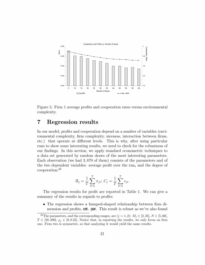
Here we look at average profits and average cooperation rates as a functionof complexity, given the degree of niceness (ρ1 = ρ2 = 0.05). We see fromFigure 5 that the more information to process (i.e., the greater environmentalcomplexity) the lower is profits and average cooperation. This finding impliesthat all else equal, the prospects for sustained cooperation is diminished incomplex environments.

6.4 Cooperation versus ’niceness’

The above results are given for symmetric firms. Here we ask the question:What does changing the ’niceness’ value for firm 1 do to cooperation ratesand profits, holding firm two’s niceness parameter constant? Figures 6 and7 show the results. Here we see that if firm 1 increases its niceness but firmtwo holds its value constant (where ρ2 = 0) then increased niceness doesnot pay. Notice, in Figure 6, that from a value of about ρ = 0.25, firm 1cooperates almost all the time. The threshold is large enough that defection

19

0.01

0.02

0.03

0.04

0.05

1 50 99 148 197 246

ρ=0 ρ=.05

Profits

time

Figure 4: Firm 1 profits over time for two ’niceness’ values. Moving Averages(25) also provided.

by the opponent never triggers a non cooperative response. This is why, insection 7, we will focus on a subsample, with ρ ∈ [0, 0.25].While firm two also increases its cooperation rate it does not do so at the

same rate as firm one. Interestingly firm one experiences a negligible changein profits, while firm two’s profits increase due to its ’defection advantage’compared to firm 1.In summary, the results of this section show that neural networks com-

peting in a duopoly setting can learn both the economic environment andthe rival’s output decisions. This learning results in increased profit overtime, but the level of profit that the two firms can achieve is a function oftheir willingness to cooperate. The ’nicer’ they are the more they can achievemutual gains to cooperation. But if their niceness threshold is relatively low,they are less likely to cooperate. This is due to the fact that since the envi-ronment state changes each period, firms will have some error in estimatingthe demand function, thus they will always have difficulty estimating therival’s true output and this will make firms more likely to defect. Finally, in-creasing environmental complexity is associated with lower profits and lowercooperation rates.

20

0.020

0.025

0.030

0.035

0.040

5 10 15 20 25 30 35 40 45 50 55 600.2

0.4

0.6

0.8

1

profits coop. ratesNumber of Inputs

Cooperation and Profits vs. Number of Inputs

Cooperation R

ate

Profit

Figure 5: Firm 1 average profits and cooperation rates versus environmentalcomplexity.

7 Regression results

In our model, profits and cooperation depend on a number of variables (envi-ronmental complexity, firm complexity, niceness, interaction between firms,etc.) that operate at different levels. This is why, after using particularruns to show some interesting results, we need to check for the robustness ofour findings. In this section, we apply standard econometric techniques toa data set generated by random draws of the most interesting parameters.Each observation (we had 3, 870 of them) consists of the parameters and ofthe two dependent variables: average profit over the run, and the degree ofcooperation:12

Πj =1

T

TXt=1

πjt; Cj =1

T

TXt=1

cjt.

The regression results for profit are reported in Table 1. We can give asummary of the results in regards to profits:

• The regression shows a humped-shaped relationship between firm di-mension and profits, cet. par. This result is robust as we’ve also found

12The parameters, and the corresponding ranges, are (j = 1, 2): Mj ∈ [2, 25], N ∈ [5, 60],T ∈ [50, 500], ρj ∈ [0, 0.25]. Notice that, in reporting the results, we only focus on firmone. Firm two is symmetric, so that analyzing it would yield the same results.

21

0.0

0.2

0.4

0.6

0.8

1.0

0 0.025 0.05 0.075 0.1 0.125 0.15 0.175 0.2 0.225 0.25

Firm 1

Firm 2

Firm 1's Cooperation Paramter

Avg. C

ooperation Rate

Cooperation Rates vs. Firm 1's Cooperation Parameter

Figure 6: Average cooperation rates for firm 1 and firm 2 versus firm 1’sniceness value.

it in our other papers under different circumstances.

• The relationship between profit and environmental complexity is neg-ative and nonlinear.

• Cet. par. increasing time increases profits since it lowers the firm’serror.

• Figure 8, where we plot profit as a function of ρ1 and ρ2, gives aninteresting example of the insights that are possible with our type ofanalysis. The relationship between profit and own willingness to coop-erate is broadly negative, even if non-linearly. Holding constant firm2’s willingness to cooperate, if we increase ρ1, firm 1 puts itself in theclassic prisoner’s dilemma situation: if the rival defects then coopera-tion will yield a lower pay-off. The non-linearity, on the other hand,is linked to uncertainty and learning: extreme types (’harsh’ or ’soft’)have a more predictable behavior; the opponent will thus be able tolearn it better, and act consequently. This will result in higher profitsfor both firms. Being in the middle, on the other hand, sends contra-dictory signals to the competitor, and does not favor learning. Such aresult would disappear were the firm acting in a world without uncer-tainty. On the other hand, increased willingness to cooperate from theopponent (larger ρ2) yields larger profits for firm 1, ceteris paribus.

22

0.020

0.025

0.030

0.035

0.040

0.045

0.000 0.025 0.050 0.075 0.100 0.125 0.150 0.175 0.200 0.225 0.250

Firm 1

Firm 2

Profits vs. Firm 1's Cooperation Parameter

Firm 1's Cooperation Parameter

Profit

Figure 7: Average profits for firm 1 and firm 2 versus firm 1’s niceness value.

Before proceeding, we can draw a first conclusion: Our model confirmsprevious findings (Barr and Saraceno, 2002; forthcoming) on the relationshipbetween firm profitability, size and the environment it faces; specifically,environmental complexity negatively affects profits, and the trade-off relativeto firm size, between speed and accuracy emerges in this setting as well, givinga hump shape relationship between firm size and profit. We also showed thatmore cooperative firms have higher profits.

We now turn to the other dependent variable, the one specific to thispaper: the degree of cooperation; the results of the regression are reportedin Table 2.The regressions yield the following results:

• As expected, the willingness to cooperate by any of the two firms in-creases the cooperation rate over the relevant range of ρ1 and ρ2.

• Also expected is the negative relationship between environmental com-plexity (N) and degree of cooperation. In a more complex environment,uncertainty makes it harder for a firm to detect defection, by the op-ponent, who has thus less incentive to cooperate.

• A more interesting picture relates the cooperation rate with firm di-mension (see fig 9). We see that after some point, an increased firmsize for the rival will induce lower cooperation for firm 1, while we see

23

Dependent Variable: 10000 ·Π1

Variable Coeff. Variable Coeff. Variable Coeff.M1 5.94

(0.738)T 3 0.000

(0.000)ρ1 −345.1

(21.8)

M2 −0.391(0.108)

T 4 0.000(0.000)

ρ2 741.7(46.1)

M21 −0.825

(0.102)N −4.18

(0.327)ρ2

1 2, 614.5(200.3)

M22 0.017

(0.004)N 2 0.172

(0.018)ρ2

2 −6, 712.7(736.5)

M31 0.034

(0.006)N 3 −0.003

(0.000)ρ3

1 −5, 313.7(531.1)

M41 −0.001

(0.000)N 4 0.000

(0.000)ρ3

2 26, 617(4399.5)

M1 ·M2 −0.029(0.003)

M1 · T 0.006(0.000)

ρ42 −38, 600

(8712.4)

T 0.778(0.049)

T ·N −0.003(0.000)

ρ1 · ρ2 −134.3(28.7)

T 2 −0.002(0.000)

M1 ·N 0.053(0.001)

cons 243.9(3.8)

R2 = 0.9351Number of obs. 3870

Table 1: Regression results. Dependent variable is profit of firm 1 (standarderrors in parentheses; non significant variables have been omitted)

a weaker, but opposite effect for firm 1’s size in its own cooperationrates. In general there is a non-linear relationship between own sizeand cooperation.

To summarize, our regressions substantially confirm the robustness of theresults of section 6: cooperation is hampered by more complex environments,and of course by lower ”niceness,” or willingness to cooperate. In addition,our regression analysis sheds light on the non-linear relationship betweenfirms sizes and cooperation.

8 Network Equilibria

Here we explore the concept of equilibrium with regards to the two importantfactors that affect performance: the choice of network size and the choice ofa niceness level. Above we explored the relationship between performance,

24

230

240

250

260

270

profit 1

00.1

0.2 rho20 0.05 0.1 0.15 0.2 0.25rho1

Figure 8: Coefficients taken from the regression presented in table 1.

and cooperation, controlling for several variables including size and niceness.Here we explore in a bit more detail the components of strategic interactionin the sense that a rival’s choice of network size and niceness affects thefirm’s pay-off, as well as cooperation rates. We explore this concept here bylooking at the equilibria that emerge over the possible range of network sizesand niceness values.We define an network equilibrium (NE) as a choice of Mj and ρj for each

firm such that neither firm has an incentive to change its network size orniceness given its rival’s choice of network size and niceness. That is to say,in an equilibrium, each network, given the number of agents (nodes) of itsrival and its rival’s niceness, finds that switching to another number of agentsand/or niceness will decrease its average (total) profit. The equilibrium is aquadruple {M∗

1 , ρ∗1,M

∗2 , ρ

∗2} such that

Πj

¡M∗

j ,M∗−j, ρ

∗j , ρ

∗−j

¢ ≥ Πj

¡Mj,M

∗−j, ρj, ρ

∗−j

¢, ∀Mj, ρj j = 1, 2.

where

Πj =1

T

TXt=1

πjt

¡Mj,M−j, ρj, ρ−j

¢.

In this section we ask: What is the relationship between environmentalcomplexity, network size, niceness, profit and cooperation rates at equilib-rium? More generally, we are interested in exploring how a firm adapts to

25

Dependent Variable: 10000 · C1

Variable Coeff. Variable Coeff. Variable Coeff.M1 −22.12

(9.88)N −6.27

(1.60)ρ2

2 −92, 069.4(24232.9)

M2 105.74(23.75)

M31 −.042

(.020)ρ3

1 1, 342, 292(139338)

M21 1.70

(.81)N 2 .049

().022ρ3

2 341, 911.8(144654.6)

M22 −12.92

(3.27)M2 ·N .149

(.040)ρ4

2 −508, 592(286234)

M32 .635

(.176)T ·N −.019

(.002)ρ4

1 −1, 559, 312(275964)

M42 −.0112

(.003)ρ1 75, 181.7

(1450.4)

ρ1 ·M1 16.56(10.22)

T 2.92(.195)

ρ2 11, 246.4(1516.3)

cons. 4.043(83.3)

T 2 −.002(.000)

ρ21 −463, 794.8

(23296.7)

R2 = .9463Number of obs: 3870

Table 2: Regression results. Dependent variable is the average cooperationrate of firm 1 (standard errors in parentheses; non significant variables havebeen omitted).

given different environmental conditions. That is, for a given environment,the firm seeks to find an optimal network configuration (size and niceness),and this search results in an accompanying profit and cooperation rate.We focus on the equilibria that exist after T periods, and we do not

examine firms changing the number of managers during the learning process.Rather we conduct a kind of comparative statics exercise, whereby we lookat the NE that arise for given environmental conditions.In this experiment, we have networks of different sizes compete for T =

250 iterations (for each set of M 0s and ρ0s and input numbers we generate30 runs and take averages to smooth out fluctuations in each run). Thatis to say, firms compete for each size, M1,M2 ∈ {2, ..., 20} , and nicenessvalue ρj =∈ {0, ..., 0.25} . We repeat this competition for different levels ofcomplexity, i.e., N = 5, 10, . . . , 30.For each complexity value we calculated the NEs that emerge (for each

number of inputs there were always more than one equilibrium) and then

26

0.4

0.41

0.42

0.43

op 1

5 10 15 20 25M1, M2

Figure 9: Cooperation rate of firm 1 as a function of M1 (thin line) and M2

(thick line). Plot coefficients from table 3.

added the total number of managers of the two firms for each equilibriumto obtain an ‘equilibrium industry size’ and averaged the ρ0s for an averageindustry niceness. This gave us a data set of 96 NEs (for an average of 16per complexity level).

Profits and Network Size The first result of this large run is consis-tent with the findings of the previous sections. Figure 10 shows that in morecomplex environments the equilibrium structure of the market entails higherfirm dimension and lower average profit.On the other hand, a clear pattern between complexity and cooperation

does not appear. The equilibrium average ρ shows a slight increase withcomplexity, going from 0.078 to 0.086. Interestingly, the degree of cooperationdoes not seem to be related to the number of inputs (Figure 11).However, if we delve more deeply into the ρ0s and cooperation rates for

the two firms, we do see the emergence of some patterns. In equilibrium apolarized behavior structure appears. In general, if one firm evolves towardsan aggressive stance (i.e., it selects a low ρ), this induces the competitor toact ’soft,’ i.e., to be more accommodating. Figure 12 shows this result.To investigate more in depth this relationship, we ran a regression with

ρ1 as the dependent variable, and the competitor’s niceness level, size, andcomplexity as independent variables. Table 4 reports the results.First, notice that the regression confirms the insignificance of environmen-

27

0.02

0.03

0.03

0.04

0.04

5 10 15 20 25 30

0

2

4

6

8

10

12

14

Profit nodes

Complexity

Nodes

Profit

Figure 10: Optimal profit and firm dimension. ’Industry’ averages.

tal complexity in explaining cooperative behavior. More surprising, firms’size also appears to be unrelated with equilibrium niceness. Coming to thedriving variable, ρ2, the regression confirms the negative relationship for bothsmall and large values of ρ2. If we take the coefficients for ρ2 and plot themagainst ρ1 (Figure13), we notice that for values of ρ2 below about 0.06 therelationship is strongly negative (which means that an aggressive behavior offirm 2 induces soft behavior of 1). Then there is a portion in which the twoare complementary, that goes to about ρ2 = 0.16, and then the two becomebasically unrelated. In other words, once firm two is sufficiently soft, firm 1becomes aggressive regardless of the value of 2In summary, we can draw the following conclusions about the network

equilibria that emerge:

• Profits in equilibrium are decreasing in complexity.

• Firm size in equilibrium is increasing.

• On, average, cooperation rates do not appear to be affected by com-plexity; despite the slight positive increase in niceness as we increasecomplexity. But complexity is strongly related to the niceness valuesof the two firms.

28

0.50

0.60

0.70

0.80

5 10 15 20 25 30

0.05

0.06

0.07

0.08

0.09

0.10

Coop rhos

Complexity

Coop

Nicen

ess

Figure 11: Equilibrium cooperation rates and niceness values. ’Industry’averages.

• Further, firms ’take sides’ in their niceness values in equilibrium. Inother words, a high nice value by one firm will have a low nice valueby another firm in equilibrium.

9 Conclusion

This paper has presented a model of firm learning and cooperation. We in-vestigate the prospects for cooperation given an agent-based model of thefirm, which must learn to map environmental signals to changing demandand its rival’s output decision. We present two sets of results: (1) outcomesof firm performance and cooperation, holding rival’s behavior constant, and(2) the equilibria that emerge due to strategic interaction. In regards to (1),we demonstrate that increased environmental complexity is associated withlower profitability and lower willingness to cooperate. In complex environ-ments frequent cooperation is more sustainable when firms are more willingto be ’nice’ in the sense that firms are less likely to defect if they estimate theirrival will defect. Further we show that firm size has an effect on both prof-its and cooperation. Increasing firm size, holding the rival’s firm constant,increases profits up to a point and then profits decrease. This trade-off is

29

Equilibrium ρ2 vs ρ1

0.04

0.06

0.08

0.10

0.12

0.14

0.04 0.05 0.06 0.07 0.08 0.09 0.10ρ1

ρ2

Trendline

Figure 12: Scatterplot of equilbrium ρ0s (average values for each compleixtylevel).

due to the fact that adding agents improves accuracy greater than the lossof speed in learning, up to a point. Increasing firm size, ceteris paribus, hasan interesting effect on cooperation: we see a non-linear relationship in thefirm’s cooperation as it increases its size; yet we see that rival’s size has ahumped-share effect on the firm’s cooperation rate.In regards to network equilibria, we have shown that increasing complex-

ity is associated with larger average firm size and lower profits in equilibrium.We do not find any relationship between cooperation and complexity, butthis is due to the fact that firm’s ’take sides’ in their niceness values. Thatis to say, in equilibrium, when one firm chooses to be aggressive, the otherresponds by being relatively nice.This paper leads to several possible research extensions. First we can

explore the prospects for cooperation given that firms play different strategiesrather than just the Tit-For-Tat type employed here. Also we can explorethe evolution of cooperation given that firms can switch strategies over time.Further we can see how the structure of the network itself affects learning andcooperation. For example, we can study how the networks behave when theyhave more than one hidden layer or when information to agents is restricted,in order to model specialization.

30

Dependent Variable: ρ1

Variable Coeff. Variable Coeff.ρ2 −6.47

(−6.52)∗N −0.0006

(−0.683)

ρ22 76.88

(4.84)∗M1 −0.0014

(−0.718)

ρ32 −355.9

(−4.07)∗M2 0.0009

(0.448)

ρ42 567.6

(3.63)∗const 0.177

(5.873)∗

R2 = 0.649Number of obs: 98

Table 3: Regression results. The dependent variable is the equilibrium nice-ness value of firm 1. t− stats in parentheses. ∗ Statiscially significant at the99% level or greater.

References

Axelrod, R. (1984). The Evolution of Cooperation. Basic Books: New York.

Axelrod, R. (1997). The Complexity of Cooperation: Agent-Based Models ofCompetition and Collaboration, Princeton University Press: Princeton.

Barr, J. and F. Saraceno (forthcoming). Cournot competition, organizationand learning. Journal of Economic Dynamics and Control.

Barr, J. and F. Saraceno (2002). A computational theory of the firm. Journalof Economic Behavior and Organization, 49, 345-361.

Carley, K. M. (1996). A Comparison of artificial and human organizations.Journal of Economic Behavior and Organization, 31, 175-191.

Cho, I.-K. (1994). Bounded rationality, neural networks and folk theorem inrepeated games with discounting. Economic Theory, 4, 935-957.

Croall, I. F. and J. P. Mason (1992). Industrial Applications of Neural Net-works: Project ANNIE Handbook, Springer-Verlag: New York.

Cyert, R.M. and M.H. DeGroot (1973). An analysis of cooperation and learn-ing in a duopoly context. American Economic Review, 63, 24-37.

31

0

0.02

0.04

0.06

0.08

0.1

0.12

0.14

0.16

0.18

rho1

0.05 0.1 0.15 0.2 0.25rho2

Figure 13: ρ1 = 0.177− 6.47ρ2 + 76.88ρ22 − 356ρ3

2 + 567.6ρ42

DeCanio, S. J. and W. E. Watkins (1998). Information processing and orga-nizational structure. Journal of Economic Behavior and Organization,36, 275-294.

Fudenberg, D. and J. Tirole (1991). Game Theory, The MIT Press: Cam-bridge.

Green, Edward and Robert Porter (1984). Noncooperative Collusion underImperfect Price Competition. Econometrica, 52:87-100.

Ho, T-H. (1996). Finite automata play repeated prisoner’s dilemma with in-formation processing costs. Journal of Economic Dynamics and Control,20, 173-207.

Holland, J. H. (1975). Adaptation in Natural and Artificial Systems, Univer-sity of Michigan Press: Ann Arbor.

Kuan C.-M. and H. White (1994). Artificial neural networks: an econometricperspective. Econometric Reviews, 13, 1-91.

Miller, J. H. (1996). The coevolution of automata in the repeated prisoner’sdilemma. Journal of Economic Behavior and Organization, 29, 87-112.

Radner, R. (1993). The organization of decentralized information processing.Econometrica, 61, 1109-1146.

32

Rubinstein, A. R. (1986). Finite automata play the repeated prisoner’sdilemma. Journal of Economic Theory, 39, 83-96.

Skapura, D. M. (1996). Building Neural Networks, Addison-Wesley: NewYork.

Tirole, J. (1988). The Theory of Industrial Organization, The MIT Press:Cambridge.

Verboven, F. (1997). Collusive behavior with heterogeneous firms. Journalof Economic Behavior and Organization, 33, 122-139.

Vriend, N. J. (2000). An illustration of the essential difference between in-dividual and social learning, and its consequences for computationalanalyses. Journal of Economic Dynamics and Control, 24, 1—19.

33