Optimization of a Pin-and-Slot Ball Valve Linkage - DSpace ...

Optimization of a Pin-and-Slot Ball Valve Linkage:with an Application to Wireline Cutting in Downhole Oil Well Tools

by

ROBERT DOWLING LENTZ

Submitted to the Department of Mechanical Engineering in partialfulfillment of the requirements for the degrees of

Master of Science in Mechanical Engineering

Bachelor of Science in Mechanical Engineering

at the

MASSACHUSETTS INSTITUTE OF TECHNOLOGYJune, 1999

@ 1999 Robert Dowling Lentz. All rights reserved

The author hereby grants MIT permission to reproduce and to distributepublicly paper and electronic copies of this document in whole or in part.

TE

2003

LIBRARIES

MASSACUSETTS INS TITUTEOF TECHNOLOGY

LIBRARIES

I A ~-.;'/

/i---

4

1/

Robert Dowling LentzDepartment of Mechanical Engineering

May 7, 1999

W Z

40 Professor Steven DubowskyProfessor of Mechanical Engineering

Thesis Supervisor

Accepted byProfessor Ain A. Sonin

Chairman, Departmental Committee on Graduate Studies

1

Author

Certified by - - I

I

Optimization of a Pin-and-Slot Ball Valve Linkage:with an Application to Wireline Cutting in Downhole Oil Well Tools

by

Robert Dowling Lentz

Submitted to the Department of Mechanical Engineering on May 7, 1999in partial fulfillment of the requirements for the degrees of Bachelor of

Science and Master of Science in Mechanical Engineering

Abstract

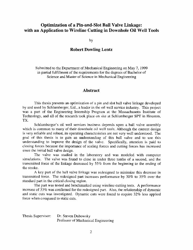
This thesis presents an optimization of a pin and slot ball valve linkage developedby and used by Schlumberger, Ltd., a leader in the oil well service industry. This projectwas a part of the Engineering Internship Program at the Massachusetts Institute ofTechnology, and all of the research took place on site at Schlumberger SPT in Houston,TX.

Schlumberger's oil well services business depends upon a ball valve assemblywhich is common to many of their downhole oil well tools. Although the current designis very reliable and robust, its operating characteristics are not very well understood. Thegoal of this thesis is to gain an understanding of this ball valve and to use thisunderstanding to improve the design of the valve. Specifically, attention is paid toclosing forces because the importance of sealing forces and cutting forces has increasedsince the initial ball valve design.

The valve was studied in the laboratory and was modeled with computersimulations. The valve was found to close in under three tenths of a second, and thetransmitted force of the linkage decreased by 55% from the beginning to the ending ofthe stroke.

A key part of the ball valve linkage was redesigned to minimize this decrease intransmitted force. The redesigned part increases performance by 30% to 35% over thestandard part in the critical closing region.

The part was tested and benchmarked using wireline cutting tests. A performanceincrease of 33% was confirmed for the redesigned part. Also, the relationship of dynamicand static cuts was investigated. Dynamic cuts were found to require 32% less appliedforce when compared to static cuts.

Thesis Supervisor: Dr. Steven DubowskyProfessor of Mechanical Engineering

2

Acknowledgements

Too many people directly or indirectly contributed to the completion of this work to

properly thank them all in this small space.

I would like to express my supreme gratitude to my Schlumberger advisor, Fred

Hernandez, without whose direction I would not have been able to complete my thesis.

He was constantly available for consultation as a friend and a mentor. I also wish to

thank Stewart Jenkins for his encouragement, friendship, and availability for discussion

about my project.

On an academic level, I would like to thank my MIT advisor Professor Steven

Dubowsky. He was especially instrumental in the final thesis write up. I would also like

to thank Professors Anna C. Thornton and Woodie Flowers for their instruction in the

principals of mechanical design.

On a professional level, I would like to thank Schlumberger Wireline and Testing

management for supporting this program and my project. Tom Zimmerman, Ashley

Kishino, Chris Spiers, and Shelby Guidry all at one time or another had to provide or

approve support for this program. I also would like to thank the following Schlumberger

managers, engineers, designers, and technicians for their help and insights over my eight

month internship: Nathan Addicks, Danny Balle, Gilbert Flores, Mimi Gonzalez, Mike

Griffith, Richard King, Ronnie Kucera, Tommy Kucera, Jason Kobersky, Leon

Mckissack, Dexter Mootoo, Vance Nixon, Dinesh Patel, Marvin Pollock, Mike Ramsey,

Gary Rytlewski, David Sewell, Chris Smith, and Mitch Wilcox. I would also like to thank

everyone else at Schlumberger SPT for a finely run research and design center that made

this project possible. Finally, I thank my officemate, roommate, and fellow 'tuna twin',

Tye Schlegelmilch, whose advice, humor, and companionship made the internship

experience an unforgettable one.

3

My thanks also go to my many friends who helped me through the hard times and helped

create the good ones. I want to give special thanks to my close friends Sumit Agarwal,

Chris Benton, Andrew Howard, Liz Montalvo, and Mads Schmidt for their invaluable

friendship and support.

I wish to thank Gordon Hamilton and Stu Schmill, my coaches while on the MIT crew

team, whose encouragement, wisdom, and guidance helped me develop skills and

qualities that have and continue to impact my life "off the water." I wish to also thank

my close friends Karl, Mike, Parker, Smitty, Karsten, Cotner, Toby, and Anand from the

boathouse who have provided the friendly competition necessary to achieve excellence.

Finally, I cannot fully express how important the love and encouragement of my parents

and brother have been to me. Thank you for instilling in me a desire to do my best and to

constantly challenge myself. I can only hope that I am able to encourage my children in

the way that you have and continue to encourage me.

4

Table of Contents

ABSTRA CT ............................................................................................................................................ 2

ACKNOW LEDG EM EN TS....................................................................................................................3

TABLE O F CO NTENTS........................................................................................................................5

LIST O F FIG URES................................................................................................................................7

LIST OF TABLES:.................................................................................................................................9

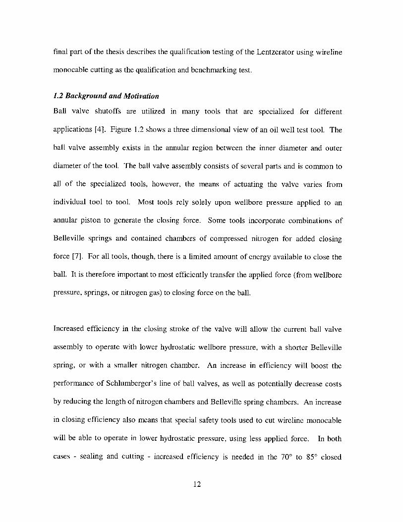
1 INTRODUC TIO N ............................................................................................................................. 10

1.1 OVERVIEW ..................................................................................................................................... 101.2 BACKGROUND AND M OTIVATION ................................................................................................. 121.3 PROJECT SUMMARY ....................................................................................................................... 14

2 CURRENT BALL VALVE DESCRIPTION ................................................................................. 17

2.1 DESCRIPTION OF PARTS................................................................................................................ 172.2 DESCRIPTION OF OPERATION.......................................................................................................... 21

3 TESTING AND SIMULATION OF BALL VALVE .................................................................... 23

3.1 EXPERIMENTAL TESTING.............................................................................................................. 243.1.1 Apparatus............................................................................................................................... 243.1.2 Velocity Tests ......................................................................................................................... 303.1.3 Cycling Tests..........................................................................................................................323.1.4 Cutting Tests .......................................................................................................................... 32

3.2 SIMULATIONS WITH WORKING MODEL-3D 4.0 ...................................... 353.2.1 General .................................................................................................................................. 353.2.2 Linear velocity to rotational velocity .................................................................................... 363.2.3 Velocity Sim ulations ............................................................................................................... 38

4 PROPERTIES OF CURRENT BALL VALVE ............................................................................. 39

4.1 APPLIED FORCE ............................................................................................................................. 394.1.1 General .................................................................................................................................. 394.1.2 Efficiency of Standard Linkage ............................................................................................ 414.1.3 Force Calculations ................................................................................................................. 42

4.2 STRESS CALCULATIONS................................................................................................................ 424.2.1 Shear Stress Calculations ....................................................................................................... 424.2.2 Bending Stress Calculations................................................................................................. 444.2.3 Contact Stress Calculations ................................................................................................ 46

4.3 DYNAMIC PROPERTIES ................................................................................................................. 484.3.1 General .................................................................................................................................. 484.3.2 Closing Time .......................................................................................................................... 484.3.3 Closing Velocity Profile .......................................................................................................... 494.3.4 Linear Velocity of Operator and Power Piston .................................................................... 504.3.5 Closing Velocity ..................................................................................................................... 52

5 RE-DESIGNED OPERATOR: LENTZERATOR.........................................................................53

5.1 DESIGN PROCESS ........................................................................................................................... 535.2 DETAILS OF DESIGN........................................................................................................................575.3 APPLIED FORCE ............................................................................................................................. 615.4 STRESS CALCULATIONS................................................................................................................65

5

5.4.1 Shear Stress Calculations ....................................................................................................... 655.4.2 Bending Stress Calculations................................................................................................. 665.4.3 Contact Stress Calculations ................................................................................................ 68

5.5 DYNAMIC PROPERTIES ................................................................................................................. 705.5.1 Predicted Closing Velocity Profile ....................................................................................... 705.5.2 Actual Closing Velocity Profile............................................................................................ 715.5.3 Comparison of Standard and Redesign Velocities................................................................ 72

6 TESTING OF LENTZERATOR PROTOTYPE .......................................................................... 74

6.1 CYCLING TESTS ............................................................................................................................. 746.2 CUTTING TESTS ............................................................................................................................. 74

6.2.1 General Procedure ................................................................................................................. 746.2.2 Wireline Monocable Properties............................................................................................. 756.2.3 Summarized Cutting Results................................................................................................. 77

7 CONCLUSIONS AND RECOM M ENDATIONS .......................................................................... 80

7.1 CONCLUSIONS................................................................................................................................ 807.2 RECOMMENDATIONS FOR FUTURE W ORK...................................................................................... 83

REFERENCES ..................................................................................................................................... 85

APPENDIX A: CUTTING TEST RESULTS.......................................................................................86

A. 1 DETAILED STATIC CUTTING TESTS .............................................................................................. 86A.2 DETAILED DYNAMIC CUTTING TESTS .......................................................................................... 87

APPENDIX B: MATLAB PROGRAMS TO INTERPRET ENCODER OUTPUT.............88

B. 1 COMPAREDATA.M - PROGRAM TO PLOT VELOCITY GRAPHS FOR GIVEN PRESSURES...................... 88B.2 REDUCEDATA.M - PROGRAM TO M ATCH DATA FILES W ITH PRESSURES........................................ 93B.3 ENCODER.M - PROGRAM TO CREATE VELOCITY GRAPHS FROM DATA FILE .................................. 95B.4 ADDDATA.M - DATA SET THAT M ATCHES DATA SETS TO PRESSURES........................................ 99

6

List of Figures

FIGURE 1.1: SCHEMATIC OF A COMMON OIL WELL TOOL WITH AN INCLUDED BALL BALVE. FIGURE FROMSCHLUMBERGER M AINTAINANCE M ANUAL [4]. ................................................................ 10

FIGURE 1.2: CROSS SECTION OF A TUBING CONVEYED TEST TOOL WITH INTEGRATED BALL VALVE. WIRELINETOOL IS SHOWN RUNNING INSIDE THE TUBING. PICTURE FROM SCHLUMBERGER MAINTENANCEM A N U A L [4 ]. ...................................................................................................................... 13

FIGURE 2.1: SCHEMATIC OF BALL VALVE ASSEMBLY. A UToCAD DRAWING FROM SCHLUMBERGERM AINTENANCE M ANUAL FOR SBSV [4]. ......................................................................... 18

FIGURE 2.2: PC T B ALL V ALVE ............................................................................................................... 19FIGURE 2.3: Y OKE OPERATOR (STANDARD)............................................................................................. 20FIGURE 2.4: SEAL R ETAINER .................................................................................................................... 21FIGURE 3.1: SCHEMATIC OF EXPERIMENTAL SETUP .............................................................................. 23FIGURE 3.2: SCHEMATIC OF ENCODER INTERFACE .................................................................................. 24FIGU RE 3.3: E N CODER PIN ....................................................................................................................... 28FIGURE 3.4: PRESS FIT OF ENCODER PIN TO BALL.................................................................................. 28FIGURE 3.5: ENCODER STAND ............................................................................................................... 29FIGURE 3.6: ANGULAR VELOCITY FROM ENCODER OUTPUT, CASE OF 3000 PSI. .................................... 32FIGURE 3.7: WORKING MODEL-3D SCREEN SHOT OF STANDARD BALL VALVE SIMULATION....................... 36FIGURE 3.8: ANGULAR VELOCITY OF BALL FOR A CONSTANT INPUT OPERATOR VELOCITY OF 1 IN/S. ........ 37FIGURE 4.1: CONTACT POINT CALCULATION FOR STANDARD BALL AND OPERATOR .............................. 40

FIGURE 4.2: CALCULATION OF MOMENT ARM LENGTH AS A FUNCTION OF 0. ......................................... 40FIGURE 4.3: CALCULATION OF APPLIED TORQUE To BALL FOR INPUT PRESSURES OF 1000 PSI TO 10,000 PSI.

.......................................................................................................................................... 4 1FIGURE 4.4: STRESS C ALCULATIONS ..................................................................................................... 43FIGURE 4.5: CALCULATIONS FOR CONTACT AREA OF STANDARD OPERATOR PINS.................................... 44FIGURE 4.6: SCHEMATIC OF CONTACT STRESS FOR A CYLINDRICAL MEMBER ON A FLAT PLANE. ............. 48FIGURE 4.7: CLOSING TIME OF PCT BALL VALVE VS. PRESSURE ........................................................... 49FIGURE 4.8: VELOCITY PROFILE OF BALL VALVE CLOSING FOR INPUT PRESSURES OF 600, 1000, 2000, AND

3 0 0 0 PSI..............................................................................................................................5 0FIGURE 4.9: VELOCITY OF YOKE OPERATOR FOR INPUT PRESSURES OF 600, 1000, 2000, AND 3000 PSI

(CALCULATED FROM ANGULAR BALL VELOCITIES)................................................................ 51FIGURE 4.10: AVERAGE LINEAR VELOCITY OF OPERATOR VS. PRESSURE. .............................................. 51FIGURE 4.11: AVERAGE AND MAXIMUM CLOSING VELOCITIES FOR PCT BALL VALVE VS. PRESSURE ...... 52FIGURE 5.1: RE-DESIGNED OPERATOR FOR INCREASED EFFICIENCY: LENTZERATOR .................................. 55FIGURE 5.2: PROPOSED 'OPTIMAL' PIN DESIGN THAT INCREASES MOMENT ARM LENGTH.......................... 56FIGURE 5.3: ITERATION OF PIN DESIGNS FROM OPTIMIZED PIN TO FINAL DESIGN. ................................. 57FIGURE 5.4: COMPARISON OF CONTACT POINT BETWEEN YOKE OPERATOR PIN AND PCT BALL .............. 59FIGURE 5.5: DETAILS OF OPERATOR PIN DESIGN ................................................................................... 60FIGURE 5.6: SCHEMATIC OF PIN LENGTH ON NEW OPERATOR ................................................................... 61

FIGURE 5.7: CALCULATION OF MOMENT ARM LENGTH AS A FUNCTION OF 0 FOR RE-DESIGNED PIN. ........... 62FIGURE 5.8: MOMENT ARM LENGTH VS. ANGULAR POSITION FOR CURRENT OPERATOR AND

L ENTZERATO R. ................................................................................................................ 63FIGURE 5.9: PERCENTAGE INCREASE OF MOMENT ARM OVER CURRENT OPERATOR VS. ANGULAR POSITION

O F B A LL . .......................................................................................................................... 64FIGURE 5.10: CENTROID AND MOMENT OF AREA CALCULATIONS FOR THE LENTZERATOR. ................... 67FIGURE 5.11: WORKING MODEL-3D SCREEN SHOT OF LENTZERATOR VELOCITY SIMULATION. ................ 71FIGURE 5.12: COMPARISON OF THEORETICAL VELOCITY PROFILE FROM WORKING MODEL WITH ACTUAL

VELOCITY PROFILES MEASURED IN THE LABORATORY FOR INPUT PRESSURES OF 1000, 2000,AND 3000 PSI (USING LENTZERATOR)................................................................................. 72

FIGURE 5.13: COMPARISON OF THE VELOCITY OF THE LENTZERATOR WITH THE STANDARD OPERATOR FORINPUT PRESSURES OF 1000 AND 3000 PSI........................................................................... 73

FIGURE 5.14: RELATIVE PERCENTAGE DIFFERENCE OF STANDARD OPERATOR TO LENTZERATOR ................ 73FIGURE 6.1: CROSS SECTION SCHEMATIC OF WIRELINE MONOCABLE. ........................................................ 75

7

FIGURE 6.2: SCHEMATIC OF SHEAR FORCE CALCULATION FOR CUTTING WIRELINE MONOCABLE................ 76FIGURE 6.3: PARTIALLY CUT W IRELINE M ONOCABLE........................................................................... 78

8

List of Tables:

TABLE 3.1: PROCEDURE FOR TESTING SBSV ........................................................................................ 30TABLE 4.1: APPLIED FORCE FOR GIVEN INPUT PRESSURES ..................................................................... 42

TABLE 4.2: SHEAR STRESS FOR GIVEN APPLIED FORCES ......................................................................... 44

TABLE 4.3: BENDING STRESSES FOR GIVEN APPLIED FORCES ................................................................ 46TABLE 4.4: HERTZIAN CONTACT STRESS FOR GIVEN APPLIED FORCES .................................................... 47TABLE 5.1: EQUIVALENT INPUT PRESSURE AND APPLIED FORCE FOR THE LENTZERATOR ........................ 64

TABLE 5.2: SHEAR STRESS FOR GIVEN APPLIED FORCES ......................................................................... 66TABLE 5.3: BENDING STRESSES FOR GIVEN APPLIED FORCES .................................................................... 68TABLE 5.4: HERTZIAN CONTACT STRESS FOR GIVEN APPLIED FORCES .................................................... 69TABLE 6.1: SUM M ARY OF C UTTING TESTS................................................................................................ 79

9

1 Introduction

1.1 Overview

Schlumberger, Ltd. is the leading oilfield services company in the world [1]. As a

services company, a major aspect of their business involves creating, maintaining, and

monitoring hydrocarbon oil and gas wells [1]. Schlumberger has a complete product line

of oil well tools that are suited for the production of hydrocarbon oil and gas wells. A

cross-sectional schematic of a common oil well tool is shown in Fig. 1.1. Since these

tools are used inside of oil well piping, oil well tools have an elongated, cylindrical shape

in order to fit inside of the pipes [2]. Specific oil well tools are specialized for functions

varying from monitoring pressures of fluids to controlling the flow of fluid [3].

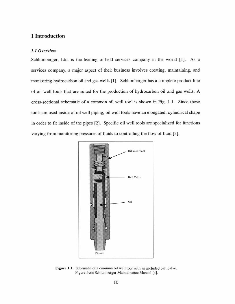
Figure 1.1: Schematic of a common oil well tool with an included ball balve.Figure from Schlumberger Maintainance Manual [4].

10

Oil Well Tool

Ball Valve

Oil

Closed

Although a variety of oil well tools will be used in a single oil well, most wells will

contain at least one tool that includes a ball valve [5]. A ball valve is a type of valve

named for the included ball (a sphere), that has a hole (cylinder) cut through the center

[5]. Figure 1.1 shows an oil well tool that includes a ball valve. When the hole is in line

with the piping, fluid can flow through the valve, but when the hole is rotated 90', fluid

cannot flow past the seal. Ball valves are useful when a large through hole is desired in

the pipe and/or high pressure needs to be sealed [3].

Schlumberger has developed several oil well tools that use ball valves. Although the

tools vary in function and form, the ball valve sub-assembly is in many of the tools [4].

Therefore, if improvements could be made to this common ball valve sub-assembly,

performance gains would be realized in several product families. The goal of this thesis

is to gain an understanding of the operation of this common ball valve sub-assembly and

redesign it in order to improve performance.

This thesis first describes the current ball valve in use by Schlumberger in terms of its

operation and strength characteristics. Since the valve had not previously been studied,

this information was unknown at the beginning of the thesis. The second part of the

thesis presents a redesign of a key part of the linkage. The redesigned part significantly

improves performance of the ball valve while adding negligible additional manufacturing

costs to the linkage. Over the design process, the redesigned part came to be called the

"Lentzerator" at Schlumberger, and that is how it will be referred to in this thesis. The

11

final part of the thesis describes the qualification testing of the Lentzerator using wireline

monocable cutting as the qualification and benchmarking test.

1.2 Background and Motivation

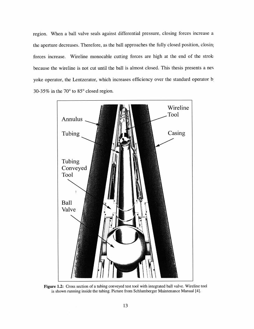
Ball valve shutoffs are utilized in many tools that are specialized for different

applications [4]. Figure 1.2 shows a three dimensional view of an oil well test tool. The

ball valve assembly exists in the annular region between the inner diameter and outer

diameter of the tool. The ball valve assembly consists of several parts and is common to

all of the specialized tools, however, the means of actuating the valve varies from

individual tool to tool. Most tools rely solely upon wellbore pressure applied to an

annular piston to generate the closing force. Some tools incorporate combinations of

Belleville springs and contained chambers of compressed nitrogen for added closing

force [7]. For all tools, though, there is a limited amount of energy available to close the

ball. It is therefore important to most efficiently transfer the applied force (from wellbore

pressure, springs, or nitrogen gas) to closing force on the ball.

Increased efficiency in the closing stroke of the valve will allow the current ball valve

assembly to operate with lower hydrostatic wellbore pressure, with a shorter Belleville

spring, or with a smaller nitrogen chamber. An increase in efficiency will boost the

performance of Schlumberger's line of ball valves, as well as potentially decrease costs

by reducing the length of nitrogen chambers and Belleville spring chambers. An increase

in closing efficiency also means that special safety tools used to cut wireline monocable

will be able to operate in lower hydrostatic pressure, using less applied force. In both

cases - sealing and cutting - increased efficiency is needed in the 700 to 85' closed

12

region. When a ball valve seals against differential pressure, closing forces increase a

the aperture decreases. Therefore, as the ball approaches the fully closed position, closin"

forces increase. Wireline monocable cutting forces are high at the end of the strok

because the wireline is not cut until the ball is almost closed. This thesis presents a neN

yoke operator, the Lentzerator, which increases efficiency over the standard operator b

30-35% in the 700 to 850 closed region.

BallValve

Figure 1.2: Cross section of a tubing conveyed test tool with integrated ball valve. Wireline toolis shown running inside the tubing. Picture from Schlumberger Maintenance Manual [4].

13

WirelineTool

Annulus

Tubing

TubingConveyedTool

The new design is compatible with the current ball valve assemblies and can be

retrofitted into existing assemblies in the field. Manufacturing the Lentzerator will be

only slightly more complicated than manufacturing the current yoke operator, so unit

costs should be very similar to current unit costs. This modification gives the greatest

amount of effect while simultaneously making the smallest amount of changes to existing

parts. The advantage of this design is that it significantly improves the operating

characteristics of the entire family of ball valves for a very low cost.

1.3 Project Summary

The first aspect of the thesis was to gain an understanding of the current ball valve

assembly in use by Schlumberger [4]. A testing apparatus was created in the laboratory

to investigate the static and dynamic properties of the valve. The ball valve linkage

transmits a non constant applied torque over the stroke of the valve. Specifically, the

amount of torque applied by the ball valve decreases by 55% over the closing stroke.

This shortcoming became the focus for the redesign. Closing times for the valve were in

the range of 0.06 - 0.30 seconds and closing velocities ranged from 400 - 2300 deg/s for

applied pressures of 500 - 10,000 psi. Stress calculations were also conducted for the

current ball valve, and simulations were run using Working Model-3D [6] to further

understand the valve.

Next, an effort was undertaken to improve the efficiency and dynamic properties of the

valve linkage by redesigning the yoke operator. The Lentzerator is the end result of this

design effort. An optimal pin geometry was identified and was iteratively improved

using dynamic analysis and computer models until the final design was reached. During

14

the design process, prototype parts were virtually simulated using Working Model-3D to

verify geometric compliance and to compare with the standard operator. Once a final,

optimal design was completed, a physical prototype was made to verify the predictions

made using the software.

Finally, qualification testing of the Lentzerator was conducted. Cycling tests were

conducted to verify that the Lentzerator would withstand numerous openings and

closings of the valve for the range of operating pressures. Also, cutting tests were

performed to compare the Lentzerator with the standard operator. Cutting tests consisted

of closing the ball valve when a wireline monocable was threaded through the inside of

the tool. The interference of the wireline monocable prevented the ball from rotating

freely past the 70' closed position. Pressure was increased on the piston until the valve

sheared the wireline monocable and was able to rotate from the 700 to the 90' closed

position. The necessary maximum input pressure force was then compared between the

two operators. The Lentzerator required 33% less applied pressure to shear the same

wireline monocable when compared to the standard operator. Less applied pressure

means that the Lentzerator is more efficient in transmitting the applied force to cutting

force.

A second set of cutting tests was also performed to compare static cuts with dynamic

cuts. Dynamic cuts used the impact loading of the rapidly closing ball valve while static

cuts were performed slowly and did not have any impact loading. Dynamic tests were

able to cut the same wireline monocable with 32% less applied force when compared

15

with static tests. The results of these tests were the same for both the standard operator

and the Lentzerator.

16

2 Current Ball Valve Description

The ball valve under examination is from the 5" Outside Diameter (OD) x 2.25" Inside

Diameter (ID) tubing conveyed testing tool family [4]. Two families of ball valves in use

at Schlumberger are the PCT, (Pressure Controlled Tester) and MFE, (Multi-Flow

Evaluator). The valves differ only in the type of ball that they use. This thesis uses the

PCT ball valve for all analysis and testing. Over the past few years, average deployment

for the PCT ball valve assembly has been 85 units per year [8]. The valve is a low

volume product which generates revenue by having a large markup. Over the past 10

years, the valve has remained fairly unchanged, but now it is the focus of investigation

[9]. Other similar valves exist for the 3" OD and 7" OD family of tools, but they are not

considered in this study.

2.1 Description of Parts

The ball valve assembly consists of roughly eight major components. The PCT ball

valve assembly is comprised of the power piston, the yoke operator, the PCT ball, the

seal retainer, the Viton or Teflon seal, the seal follower, the seal retainer spring, and the

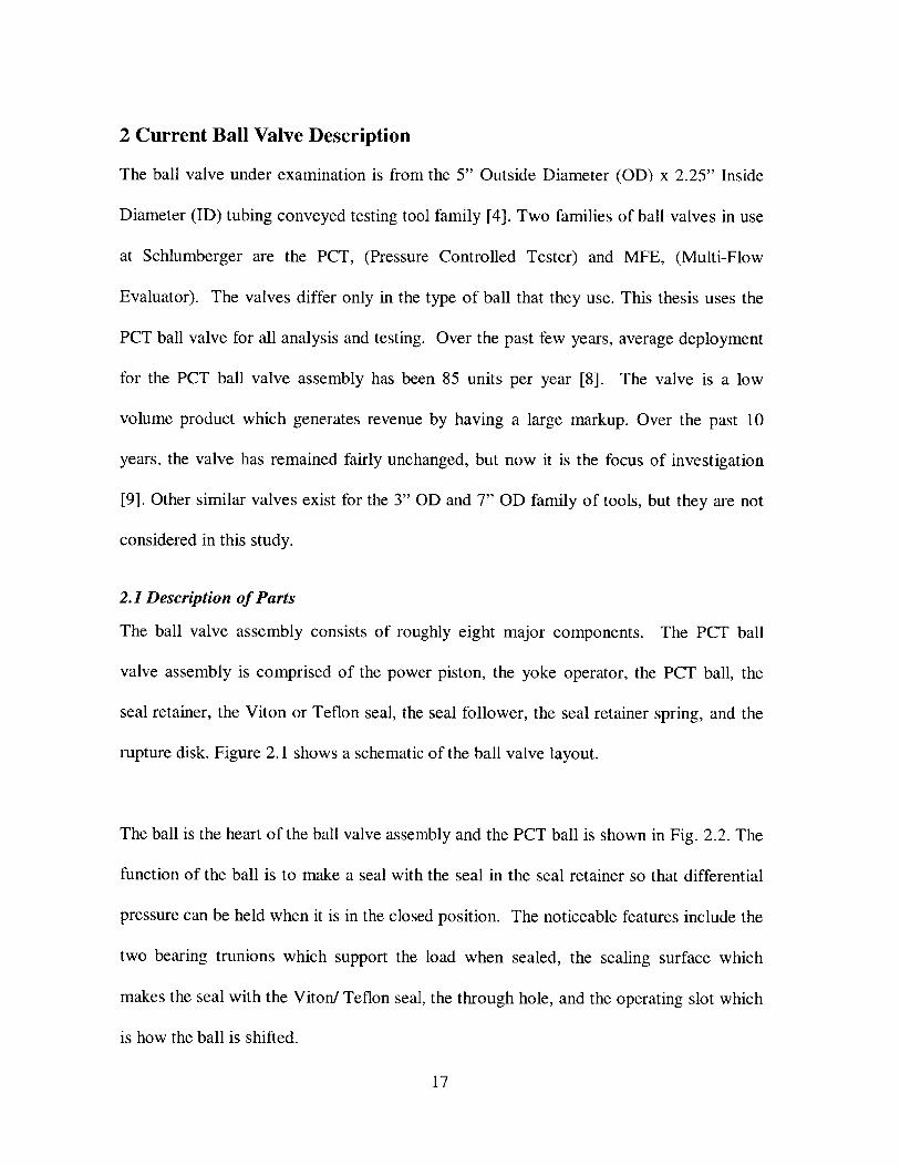
rupture disk. Figure 2.1 shows a schematic of the ball valve layout.

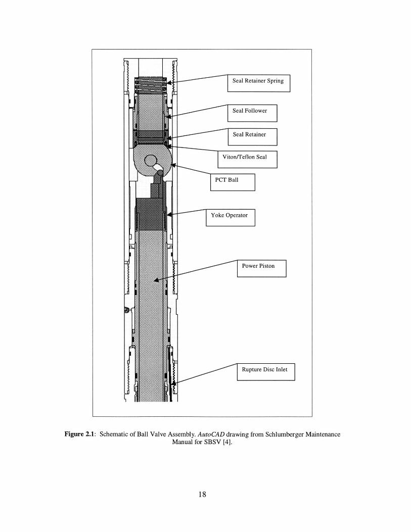
The ball is the heart of the ball valve assembly and the PCT ball is shown in Fig. 2.2. The

function of the ball is to make a seal with the seal in the seal retainer so that differential

pressure can be held when it is in the closed position. The noticeable features include the

two bearing trunions which support the load when sealed, the sealing surface which

makes the seal with the Viton/ Teflon seal, the through hole, and the operating slot which

is how the ball is shifted.

17

Rupture Disc Inlet

Figure 2.1: Schematic of Ball Valve Assembly. AutoCAD drawing from Schlumberger MaintenanceManual for SBSV [4].

18

Through Hole

Sealing Sur face

Operator Slo

Figure 2.2: PCT Ball Valve

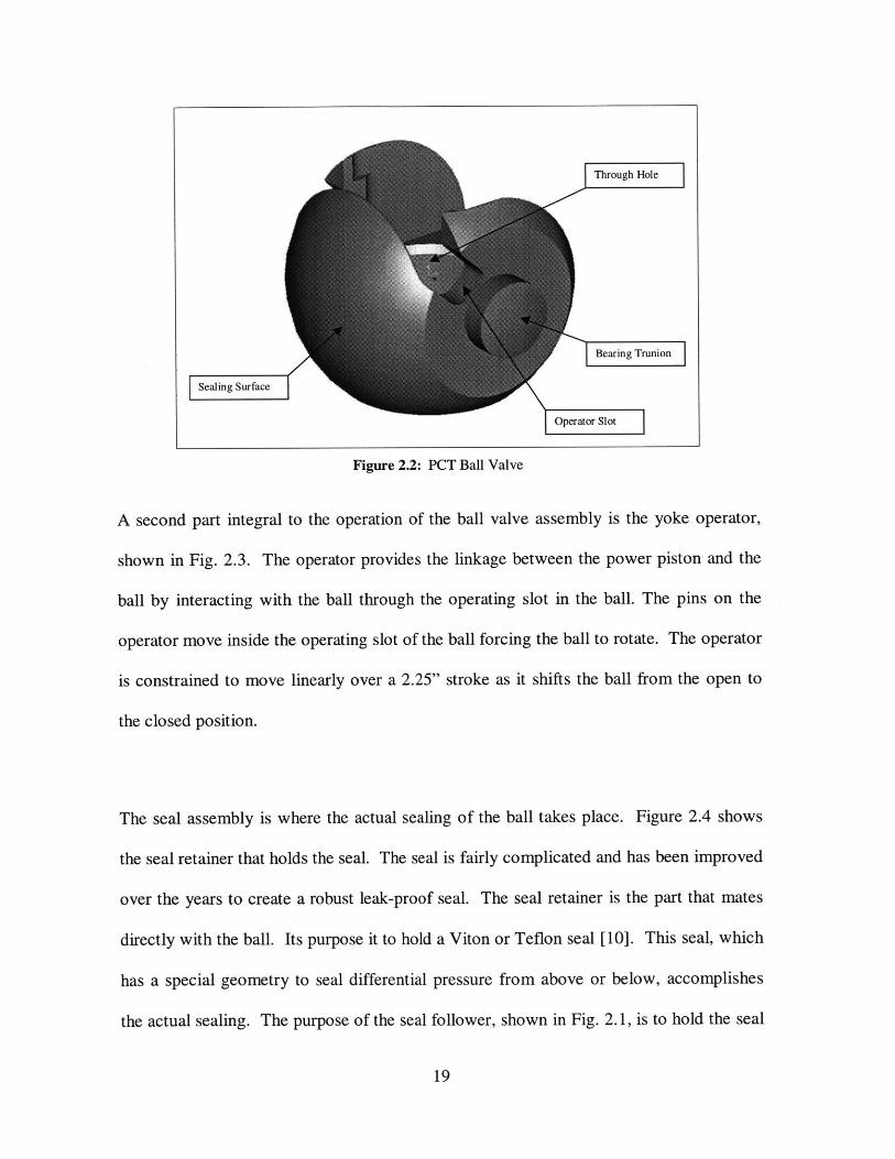
A second part integral to the operation of the ball valve assembly is the yoke operator,

shown in Fig. 2.3. The operator provides the linkage between the power piston and the

ball by interacting with the ball through the operating slot in the ball. The pins on the

operator move inside the operating slot of the ball forcing the ball to rotate. The operator

is constrained to move linearly over a 2.25" stroke as it shifts the ball from the open to

the closed position.

The seal assembly is where the actual sealing of the ball takes place. Figure 2.4 shows

the seal retainer that holds the seal. The seal is fairly complicated and has been improved

over the years to create a robust leak-proof seal. The seal retainer is the part that mates

directly with the ball. Its purpose it to hold a Viton or Teflon seal [10]. This seal, which

has a special geometry to seal differential pressure from above or below, accomplishes

the actual sealing. The purpose of the seal follower, shown in Fig. 2.1, is to hold the seal

19

retainer in place and to add a downward sealing force in proportion to hydrostatic

pressure due to differential area on the seal follower. The seal retainer spring applies a

constant downward sealing force independent of hydrostatic pressure. The seal follower

also communicates the force from the seal retainer spring to the seal retainer. The power

piston is directly connected to the yoke operator and provides the linear movement of the

yoke. The power piston is actuated by applying pressure to its integral annular piston.

Figure 2.3: Yoke Operator (standard)

20

Operator Pin

Through Hole

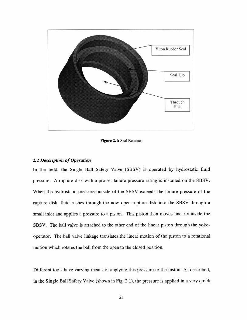
Figure 2.4: Seal Retainer

2.2 Description of Operation

In the field, the Single Ball Safety Valve (SBSV) is operated by hydrostatic fluid

pressure. A rupture disk with a pre-set failure pressure rating is installed on the SBSV.

When the hydrostatic pressure outside of the SBSV exceeds the failure pressure of the

rupture disk, fluid rushes through the now open rupture disk into the SBSV through a

small inlet and applies a pressure to a piston. This piston then moves linearly inside the

SBSV. The ball valve is attached to the other end of the linear piston through the yoke-

operator. The ball valve linkage translates the linear motion of the piston to a rotational

motion which rotates the ball from the open to the closed position.

Different tools have varying means of applying this pressure to the piston. As described,

in the Single Ball Safety Valve (shown in Fig. 2.1), the pressure is applied in a very quick

21

Viton Rubber Seal

Seal Lip

ThroughHole

manner by rupturing a rupture disc. Other tools use nitrogen instead of wellbore fluid, or

use a combination of spring action and wellbore fluid action [4, 7]. Still other tools dump

the pressure to the piston much less rapidly than the Single Ball Safety Valve, so the

actuation is slower.

22

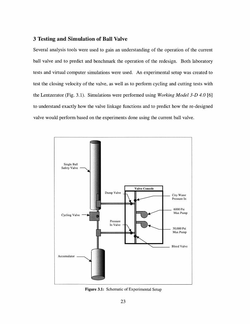
3 Testing and Simulation of Ball Valve

Several analysis tools were used to gain an understanding of the operation of the current

ball valve and to predict and benchmark the operation of the redesign. Both laboratory

tests and virtual computer simulations were used. An experimental setup was created to

test the closing velocity of the valve, as well as to perform cycling and cutting tests with

the Lentzerator (Fig. 3.1). Simulations were performed using Working Model 3-D 4.0 [6]

to understand exactly how the valve linkage functions and to predict how the re-designed

valve would perform based on the experiments done using the current ball valve.

Single BallSafety Valve

Valve ConsoleDump Valve--CtWae

Pressure In

6000 Psi

Cycling Valve Max Pump

PressureIn Valve

30,000 PsiMax Pump

Bleed Valve

Accumulator

Figure 3.1: Schematic of Experimental Setup

23

3.1 Experimental Testing

3.1.1 Apparatus

A schematic shown in Fig. 3.1 shows the experimental setup used to test the Single Ball

Safety Valve. Since this ball valve had not been previously studied in the laboratory, the

experimental setup had to be designed and built as a part of this project. Although this

ball valve assembly is used in many different tools, tests were only run on one tool. Tests

were conducted using the Single Ball Safety Valve (SBSV) tool because this tool is the

simplest and most common implementation of the ball valve assembly [4].

The experimental tests were designed so that they simulated the rapid releasing of

wellbore pressure through a rupture disc, as the valve would normally see in the field. A

one-gallon accumulator was used to simulate the reservoir of high pressure wellbore fluid

(up to 10,000 psi), and a pneumatically controlled dump valve was used to control fluid

flow into the Single Ball Safety Valve, simulating the rupturing of the rupture disc.

Ball Encoder CouplingPin

SBSV Encoder OpticalHousing Stand Encoder

Figure 3.2: Schematic of Encoder Interface

24

Tests were conducted in the high pressure test bay in the sub-sea group of

Schlumberger's Perforating and Testing Center in Rosharon, TX. The high pressure bay

is enclosed by thick concrete walls and steel doors so that high pressure tests (greater

than 7500 psi) can be conducted safely. There is a valve console that is integral to the

bay that allows the operator to remotely control a high pressure pump, a low pressure

pump, and several flow control valves. The valve console is shown in Fig. 3.1. The high

pressure is pump rated to 30,000 psi and the low pressure pump is rated to 6000 psi.

Tubing and appropriate connectors were specified and ordered so that the valve console

could be interfaced to the Single Ball Safety Valve, accumulator, and dump valve. In

addition, the ball valve was interfaced with an optical encoder so that the angular position

of the ball could be measured (see Fig. 3.2). In order to connect the encoder to the ball

valve, a physical interface had to be designed. This encoder interface consisted of an

encoder pin, a coupling, the encoder, and the encoder stand. A digital oscilloscope was

used to record the output of the encoder, and the data files were analyzed using programs

written in Matlab. The details of the apparatus will be discussed in the next sections.

3.1.1.1 Valve Console

The valve console has controls for several valves and two pumps and is depicted in Fig.

3.1. The Water Valve controls the flow of city water pressure into the valve console.

The water must be on in order for any pumps to operate. The Bleed Valve controls the

bleeding of pressure to an atmospheric waste chamber. This valve is used to release

pressure from the valve console after a test has been run. The Pressure Valve controls

flow into the line of tubing that is connected to the accumulator side of the cycling valve,

25

and the Dump Valve controls flow into the line of tubing connected to the SBSV side of

the cycling valve. Using the pneumatically controlled cycling valve, pressurized water

can be pumped into or released from either the accumulator or the SBSV using the valves

in the valve console.

3.1.1.2 Accumulator

The accumulator used for these tests is a one gallon Tobul accumulator model number

8A100-8-WS-A-MP9-MP4. The accumulator has a rating of 10,000 psi. The accumulator

is operated by pre-charging the back side of the piston with nitrogen gas to one half of the

operating pressure that is required on the water side of the piston. For example, if the

working pressure of the water in the tubing is 8,000 psi, then the back side of the

accumulator should be pre-charged with 4,000 psi nitrogen.

3.1.1.3 Tubing

The tubing used is 3/8" OD low-pressure Autoclave, part number Autoclave-MS15-084

[11]. This is the largest internal diameter tubing commercially available that is rated to

10,000 psi working pressure, a constraint of the experiment [11, 12]. A large internal

diameter is preferred so that flow restrictions are minimized.

3.1.1.4 Cycling Valve

The cycling valve is a pneumatically controlled Autoclave needle valve, part number

Autoclave-20SC9. The valve is rated to 20,000 psi and has 9/16" medium pressure

Slimline Autoclave fittings. Using a ball valve shut off with a long pneumatic hose, the

26

cycling valve can be remotely operated, and controlled safely from outside the High

Pressure Bay.

3.1.1.5 Optical Encoder

The optical encoder used is a high precision industrial optical encoder made by Encoder

Technology [13]. The encoder has a resolution of 1024 bits per revolution and a

frequency response of 125 kHz. It requires an input power of 7-24 V DC. The shaft is a

standard " diameter by %" length. A schematic of the encoder can be seen in Fig. 3.2.

3.1.1.6 Coupling

A mechanical coupling is used to couple the encoder shaft to the encoder pin. The main

purpose of the coupling is to accommodate any eccentricities between the encoder shaft

and the encoder pin. The coupling is made by Heli-Cal and is part number HCR087-88

[14]. The coupling can withstand a maximum torque that is much greater than can be

applied by the encoder. Also, the coupling will deflect less than 0.1 degrees at maximum

acceleration of the encoder. A schematic of the coupling can also be seen in Fig. 3.2.

3.1.1.7 Encoder Pin

The encoder pin, shown in Fig. 3.3, was designed as a part of the thesis and was

manufactured by Wadko Precision, Inc. The encoder pin physically connects the encoder

and the ball inside the ball valve assembly of the SBSV. One end of the encoder pin is

press fit into a hole in the ball, shown in Fig. 3.4, and the other end attaches to the

coupling, which is in turn attached to the encoder. The outside diameter of the encoder

pin is threaded so that it can be removed from the press fit. When the encoder pin is to be

27

removed from the ball, a nut is threaded onto the threaded OD of the pin so that when the

nut is tightened, the pin is pulled out of the press fit.

Figure 3.3: Encoder Pin

Figure 3.4: Press Fit of Encoder Pin to Ball

28

3.1.1.8 Encoder Stand

The encoder stand, shown in Fig. 3.5, was designed as a part of this thesis and was

manufactured by G & H Manufacturing. The purpose of the stand is to attach to the

encoder and hold it firmly to the outside of the SBSV. It is held on to the SBSV with

hose clamps that can be tightened around the outside diameter of the SBSV. Access holes

were designed into the sides of the stands so that the coupling and encoder could be

attached to the encoder pin.

Figure 3.5: Encoder Stand

29

3.1.1.9 Digital Oscilloscope

A high-end digital oscilloscope was used to capture the output data from the optical

encoder because a sampling rate of 300kHz was need to capture the output of the

encoder. The scope was a Tektronix TDS 644B [15]. The main features are that it can

store 15,000 points in memory and sample at up to 1 GHz. Also, it has a 3 inch floppy

drive so that data can be stored and transferred to a computer for analysis and archive.

3.1.2 Velocity Tests

Velocity tests were conducted using the apparatus previously described. The result of

these tests is an angular velocity profile of the ball as a function of angular position. A

procedure shown in Table 3.1 was used for each experiment, so that all tests were run in a

repeatable manner.

Pre-Test Setup Post-Test Reset

1. Bleed Closed 1. Close Cycling Valve2. Water On 2. Bleed Air on Cycling Valve3. Dump Closed 3. Save Waveform on Scope4. Cycling Closed e Verify 'Matlab' format5. Pressure Valve Open 4. Record Test Params. In Lab Book6. Pump #1/#2 On 5. Close Pressure Valve - Off7. Scope Setup 6. Open Dump Valve - On

e Single Sequence 7. Turn Water Offe Trig. On Channel 1 8. Open Bleed Valve* 15,000 pts 9. Shift Ball with Nitrogen

e Hit 'RUN' Button 10. Re-open Nitrogen Line to Atm. Press.8. Power on Encoder Switch9. Open Cycling Valve

Table 3.1: Procedure for Testing SBSV

The testing procedure consisted of first pressuring the accumulator up to the testing

pressure. After the pressure in the accumulator stabilized, the cycling valve was opened

30

so that the accumulated pressure could rush into the valve and shift the power piston up,

rotating the ball and encoder 900. The closing data was recorded with the oscilloscope

and saved to a data file in 'Matlab' format.

Pressures ranging from 500 psi to 10,000 psi in increments of 500 psi were tested. Two

measurements at each pressure were made for verification purposes. Once all of the data

was collected on the main computer, four programs were written in Matlab scripting

language to automate the analysis of the output waveform from the encoder (see

Appendices B1 - B4) [16]. The program in Appendix B.3, encoder.m, analyzes the

square wave output from the encoder and calculates an angular position vs. time graph.

The program then differentiates the position graph to calculate a velocity graph. A

sample graph of the output from this program is shown in Fig. 3.6 for the case of 3000

psi input pressure. The other three programs manage the 109 data sets so that different

initial pressure runs can be plotted versus each other.

31

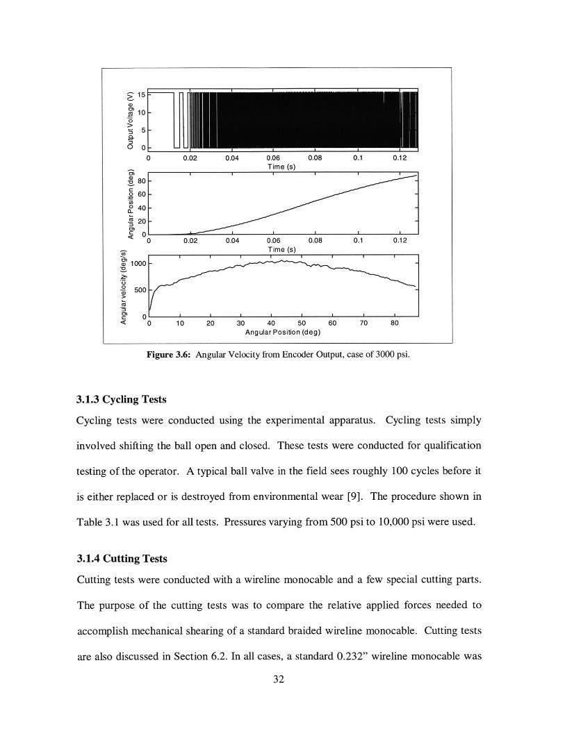
Figure 3.6: Angular Velocity from Encoder Output, case of 3000 psi.

3.1.3 Cycling Tests

Cycling tests were conducted using the experimental apparatus. Cycling tests simply

involved shifting the ball open and closed. These tests were conducted for qualification

testing of the operator. A typical ball valve in the field sees roughly 100 cycles before it

is either replaced or is destroyed from environmental wear [9]. The procedure shown in

Table 3.1 was used for all tests. Pressures varying from 500 psi to 10,000 psi were used.

3.1.4 Cutting Tests

Cutting tests were conducted with a wireline monocable and a few special cutting parts.

The purpose of the cutting tests was to compare the relative applied forces needed to

accomplish mechanical shearing of a standard braided wireline monocable. Cutting tests

are also discussed in Section 6.2. In all cases, a standard 0.232" wireline monocable was

32

threaded inside of the SBSV so that the ball would not close until the monocable had

been sheared and had moved out of the way [17]. A tension of 130 lbs was applied to the

monocable so that it was pulled taught. The reason 130 lbs. was used for the weight was

because the average tool that will be run through the ball valve weighs about 130 pounds

[9].

Now, two types of cutting tests were performed: static and dynamic. Static tests were

conducted by slowly pressuring the power piston until there was enough applied force to

shear the wireline monocable and cut. Dynamic tests were conducted by pressuring the

accumulator to a given pressure and cycling it rapidly to the power piston. When the ball

hit the monocable in dynamic tests, it had angular momentum as well as linear

momentum of the power piston to generate impact forces. The results of the dynamic

tests were a simple cut/ no cut for a given initial pressure on the accumulator. Effort was

made to zero in on the pressure needed to just cut the wireline monocable.

Three combinations of four parts were used in the cutting tests and will be described in

the next sections: (1) the standard ball with standard seal retainer, (2) the cutting ball with

cutting sleeve, and (3) the standard ball with cutting sleeve. A combination of the cutting

ball and standard seal was not used because the sharp edge on the cutting ball would

destroy the rubber seal in the seal retainer

3.1.4.1 Standard Ball with Seal Retainer

The standard ball with seal retainer was designed to seal and not to cut. As a result, the

seal retainer is made out of a soft steel and the ball has a rounded edge. The rounded

33

edge on the ball lip is critical because it slides over the rubber seal in the seal retainer

when the ball closes. Since this combination of standard ball with seal retainer was not

optimized for cutting, it was unable to cut the wireline, and as a result, this combination

was used in a limited number of cutting tests.

3.1.4.2 Cutting Ball with Cutting Sleeve

Most cutting tests were completed using a specially designed cutting sleeve that replaced

the seal retainer, seal follower, upper cage, and seal retainer spring [18]. Also, a special

cutting ball with a sharp edge was used. Dinesh Patel, a Schlumberger engineer, had

previously designed the cutting sleeve and cutting ball [18]. One of the advantages of the

cutting sleeve and ball is that they are made out of steel that has been gas nitrided, so they

have a hardness on the order of on the order of 55-59 HRC. Secondly, the cutting sleeve

is not spring mounted, so it will not deflect out of the way like the spring mounted seal

retainer will. Finally, the cutting sleeve has a much sharper edge than the seal retainer,

and there is a constant fixed gap between the ball and cutting sleeve so that the wire

cannot slip between them.

3.1.4.3 Standard Ball with Cutting Sleeve

Combinations of the standard ball with cutting sleeve were run to determine the

effectiveness of the cutting ball versus the standard ball. Fewer tests were run with this

combination than with the cutting ball combination because the standard ball is not as

hard as the cutting ball and would not withstand as many cuts.

34

3.2 Simulations with Working Model-3D 4.0

3.2.1 General

To understand the motion and dynamics of the ball valve assembly, the key parts of the

assembly were modeled in Pro/ENGINEER, a solid modeling software package [19].

The solid parts were then exported to Working Model-3D 4.0, a dynamics simulation

package [6]. A sample screen shot of Working Model-3D is shown in Fig. 3.7 for the

standard ball valve. Once in Working Model-3D, the parts were appropriately

constrained so they moved in the same directions and distances as the corresponding

physical parts. Inputs were then given to the system, and output angular velocities and

positions were measured. It is important to note that the inputs used in the simulation

were actually calculated from data obtained from the laboratory setup. The experimental

data was synchronized with the simulation data and verified to be correct. Then the

designs of the ball valve components were altered and re-exported to Working Model-3D.

Predicted values can then be accurately calculated for the new design. In this manner,

designs could then be virtually prototyped and tested using the simulation software.

Finally, when a final concept is selected, a physical prototype can be made to verify the

predictions of the simulation software, thus bypassing physical mock-ups and concept

prototypes.

35

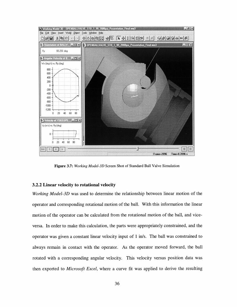
Figure 3.7: Working Model-3D Screen Shot of Standard Ball Valve Simulation

3.2.2 Linear velocity to rotational velocity

Working Model-3D was used to determine the relationship between linear motion of the

operator and corresponding rotational motion of the ball. With this information the linear

motion of the operator can be calculated from the rotational motion of the ball, and vice-

versa. In order to make this calculation, the parts were appropriately constrained, and the

operator was given a constant linear velocity input of 1 in/s. The ball was constrained to

always remain in contact with the operator. As the operator moved forward, the ball

rotated with a corresponding angular velocity. This velocity versus position data was

then exported to Microsoft Excel, where a curve fit was applied to derive the resulting

36

W IN - ---- -- --------- - Ngo

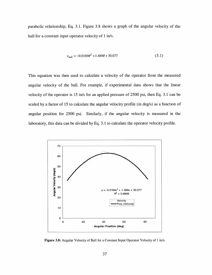
parabolic relationship, Eq. 3.1. Figure 3.8 shows a graph of the angular velocity of the

ball for a constant input operator velocity of 1 in/s.

vball = -0.0 16902 + 1.4890 + 30.077 (3.1)

This equation was then used to calculate a velocity of the operator from the measured

angular velocity of the ball. For example, if experimental data shows that the linear

velocity of the operator is 15 in/s for an applied pressure of 2500 psi, then Eq. 3.1 can be

scaled by a factor of 15 to calculate the angular velocity profile (in deg/s) as a function of

angular position for 2500 psi. Similarly, if the angular velocity is measured in the

laboratory, this data can be divided by Eq. 3.1 to calculate the operator velocity profile.

70-

60 -

50-

40-

30-

20-

10

0-0 20 40 60

Angular Position (deg)

80

37

y = -0.0169x2 + 1.489x + 30.077

Ff = 0.9898

Velocity-Poly. (Velocity)

Figure 3.8: Angular Velocity of Ball for a Constant Input Operator Velocity of 1 in/s.

--------------------------------------------

3.2.3 Velocity Simulations

Once the linear velocities of the operator were calculated from the experimental data,

they could be used as inputs for the simulations in Working Model-3D. Therefore, the

velocity profiles in the simulation could be calculated for the prototype design. The

velocity profile could then be optimized by changing the ball slot and operator pins in

Pro/ENGINEER until a desirable shape is achieved.

38

4 Properties of Current Ball Valve

4.1 Applied Force

4.1.1 General

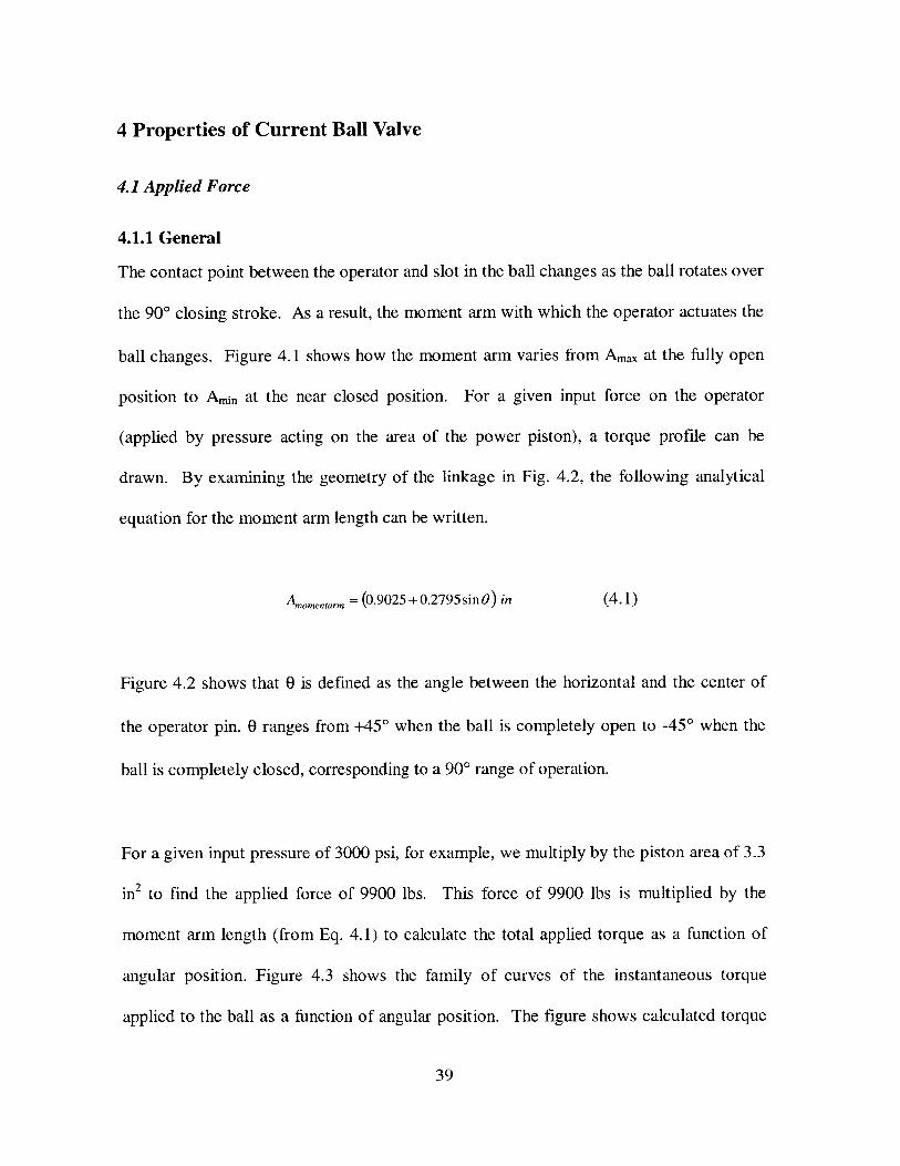
The contact point between the operator and slot in the ball changes as the ball rotates over

the 900 closing stroke. As a result, the moment arm with which the operator actuates the

ball changes. Figure 4.1 shows how the moment arm varies from Amax at the fully open

position to Amin at the near closed position. For a given input force on the operator

(applied by pressure acting on the area of the power piston), a torque profile can be

drawn. By examining the geometry of the linkage in Fig. 4.2, the following analytical

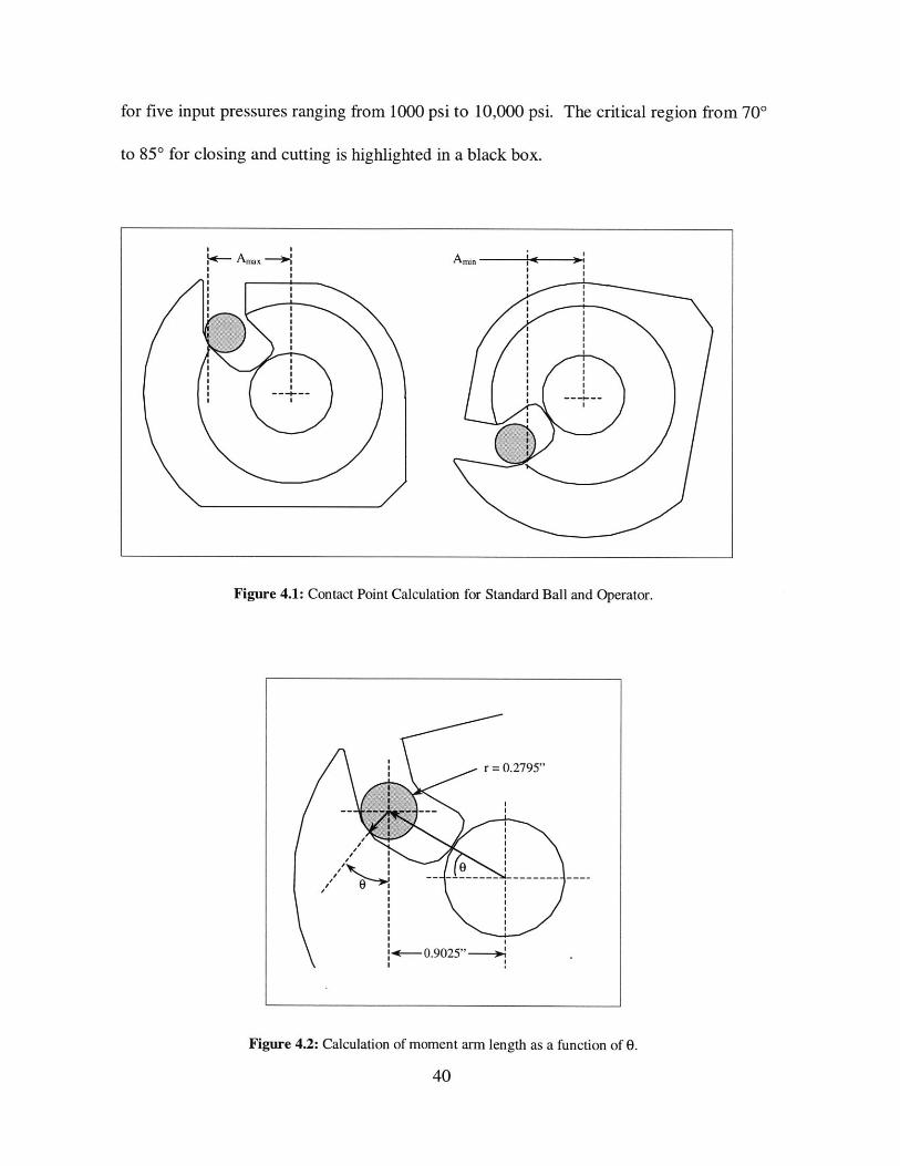
equation for the moment arm length can be written.

Amomentarm = (0.9025+0.2795sin6) in (4.1)

Figure 4.2 shows that 0 is defined as the angle between the horizontal and the center of

the operator pin. 0 ranges from +45' when the ball is completely open to -45' when the

ball is completely closed, corresponding to a 90' range of operation.

For a given input pressure of 3000 psi, for example, we multiply by the piston area of 3.3

in 2 to find the applied force of 9900 lbs. This force of 9900 lbs is multiplied by the

moment arm length (from Eq. 4.1) to calculate the total applied torque as a function of

angular position. Figure 4.3 shows the family of curves of the instantaneous torque

applied to the ball as a function of angular position. The figure shows calculated torque

39

for five input pressures ranging from 1000 psi to 10,000 psi. The critical region from 70'

to 85' for closing and cutting is highlighted in a black box.

Figure 4.1: Contact Point Calculation for Standard Ball and Operator.

Figure 4.2: Calculation of moment arm length as a function of 0.

40

~-Amex

/I

4.1.2 Efficiency of Standard Linkage

It can be seen from Fig. 4.1 and Fig. 4.3 that the linkage transfers a non-constant torque

to the ball as the angular position of the ball changes. The ratio of the applied torque to

the closing torque can be defined as the efficiency of the linkage. The applied torque

decreases by 55% from the beginning of the stroke at Amax to the end of the stroke at

Amin. The applied torque changes because the contact point between the yoke operator pin

and the ball operator slot changes. As the contact point moves closer to the center of

rotation of the ball, the effective moment arm decreases. Over the stroke of the operator,

the moment arm decreases, therefore causing the applied torque to decrease. For a

constant applied force, we can see that the efficiency of the valve is 55% less at the end

of the stroke when compared to the beginning of the stroke, because the applied torque

has decreased by 55% while the closing torque needed has remained constant.

40000---------- 10000 Psi

- 7000 Psi35000 - -- 5000 Psi

- - - -3000 Psi1000Psi

30000 --

S25000 critical region

S20000

0015000

00

000

0 15 30 45 60 75 90

Angular Position of Ball (deg)

Figure 4.3: Calculation of Applied Torque to Ball for input pressures of 1000 Psi to 10,000 Psi.

41

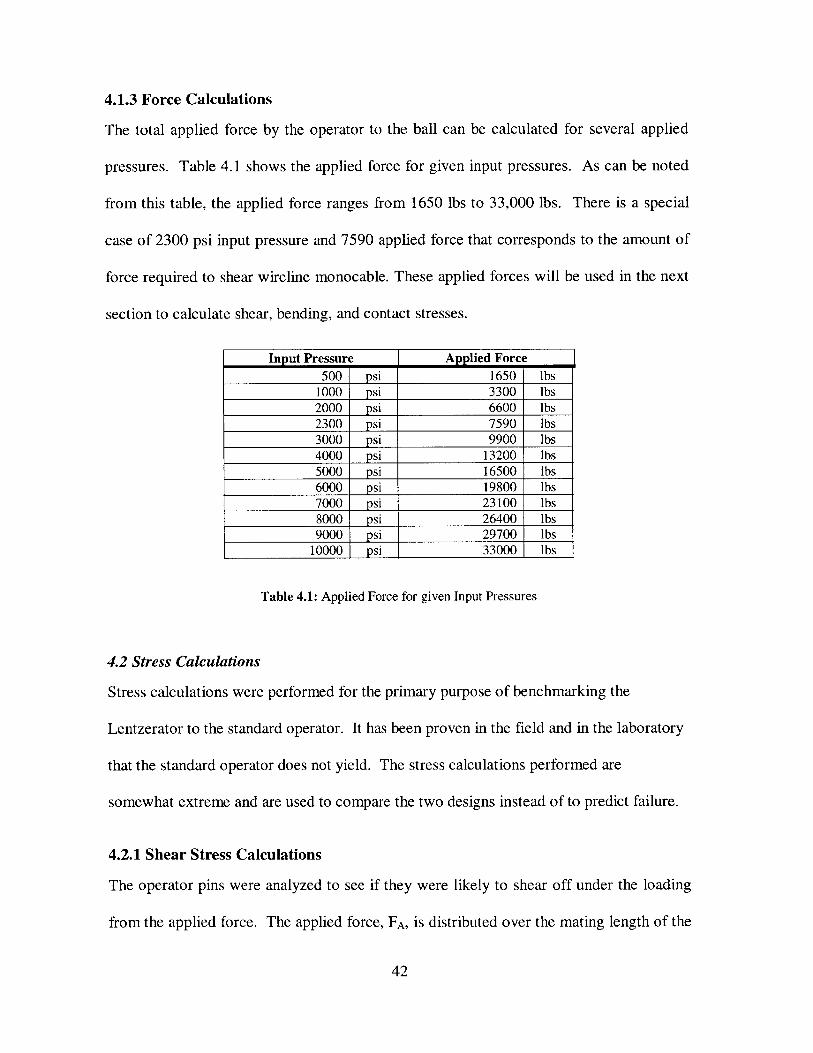
4.1.3 Force Calculations

The total applied force by the operator to the ball can be calculated for several applied

pressures. Table 4.1 shows the applied force for given input pressures. As can be noted

from this table, the applied force ranges from 1650 lbs to 33,000 lbs. There is a special

case of 2300 psi input pressure and 7590 applied force that corresponds to the amount of

force required to shear wireline monocable. These applied forces will be used in the next

section to calculate shear, bending, and contact stresses.

Input Pressure Applied Force500 psi 1650 lbs

1000 psi 3300 lbs2000 psi 6600 lbs2300 psi 7590 lbs3000 psi 9900 lbs4000 psi 13200 lbs5000 psi 16500 lbs6000 psi 19800 lbs7000 psi 23100 lbs8000 psi 26400 lbs9000 psi 29700 lbs

10000 psi 33000 lbs

Table 4.1: Applied Force for given Input Pressures

4.2 Stress Calculations

Stress calculations were performed for the primary purpose of benchmarking the

Lentzerator to the standard operator. It has been proven in the field and in the laboratory

that the standard operator does not yield. The stress calculations performed are

somewhat extreme and are used to compare the two designs instead of to predict failure.

4.2.1 Shear Stress Calculations

The operator pins were analyzed to see if they were likely to shear off under the loading

from the applied force. The applied force, FA, is distributed over the mating length of the

42

two pins. If each pin has a length of L, then the resultant force acts at a distance L/2 from

the end of the pin with magnitude FA/2, Fig. 4.4. A simple shear model was used to

calculate the shear stress on each pin [20]:

F-A (4.2)2 A

where A is the cross-sectional area of the pin contact. For a given applied force, FA, the

shear stress is a function of only the cross sectional area of the pins, A. Since there are

chamfers around the place where the pin makes contact with the operator, the cross

sectional contact area of the pin is non-circular. The area was calculated using a function

in AutoCAD to be 0.2168 in2. Figure 4.5 shows the results of the AutoCAD calculation.

For the given applied pressures, this corresponds to the shear stresses shown in Table 4.2.

As can be seen, the shear stress varies from 3805 psi to 76.1 ksi. All but the highest three

values are below the failure stress of the material, ay/2, or 57.5ksi for 17-4 PH Stainless

Steel [21].

F F

2 2

L L

- 2m2| 2

igi 4 ions

Figure 4.4: StesCluain

43

Applied Force Shear Stress1650 lbs 3,805 psi3300 lbs 7,611 psi6600 lbs 15,221 psi7590 lbs 17,505 psi9900 lbs 22,832 psi

13200 lbs 30,443 psi16500 lbs 38,054 psi19800 lbs 45,664 psi23100 lbs 53,275 psi26400 lbs 60,886 psi29700 lbs 68,496 psi33000 lbs 76,107 psi

Table 4.2: Shear Stress for given Applied Forces

of AreaCentroid/MomentStandard

A 0.2168 in"2Ix 0.00401650Iv 0.00350466

^4^4

.2793

Figure 4.5: Calculations for contact area of standard operator pins.

4.2.2 Bending Stress Calculations

Tensile and compressive stresses were calculated for the pins using Eq. 4.3:

Mc (4.3)

where M is the applied moment, c is the maximum distance from the centroid and I, is the

.2446

Design

inin

moment of area about the y axis, at the centroid [22, 23].

44

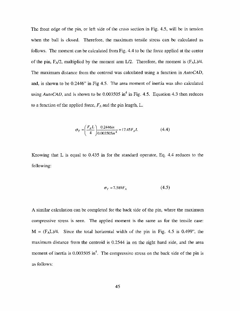
The front edge of the pin, or left side of the cross section in Fig. 4.5, will be in tension

when the ball is closed. Therefore, the maximum tensile stress can be calculated as

follows. The moment can be calculated from Fig. 4.4 to be the force applied at the center

of the pin, FA/2, multiplied by the moment arm L/2. Therefore, the moment is (FAL)/4.

The maximum distance from the centroid was calculated using a function in AutoCAD,

and, is shown to be 0.2446" in Fig 4.5. The area moment of inertia was also calculated

using AutoCAD, and is shown to be 0.003505 in 4 in Fig. 4.5. Equation 4.3 then reduces

to a function of the applied force, FA and the pin length, L.

a'r = ) 0.2446in 4 = 17.45FA L (4.4)4 0.003505in

Knowing that L is equal to 0.435 in for the standard operator, Eq. 4.4 reduces to the

following:

UTr = 7 .5 8 9 FA (4.5)

A similar calculation can be completed for the back side of the pin, where the maximum

compressive stress is seen. The applied moment is the same as for the tensile case:

M = (FAL)/4. Since the total horizontal width of the pin in Fig. 4.5 is 0.499", the

maximum distance from the centroid is 0.2544 in on the right hand side, and the area

moment of inertia is 0.003505 in4. The compressive stress on the back side of the pin is

as follows:

45

C= FAL 0.2544in 18.15FAL = 7.893F . (4.6)4 )0.003505in 4

A summary of the bending stresses vs. applied force is shown in Table 4.3. By

inspection, the theory predicts that the pins will fail due to bending stress for applied

pressures greater than 4000 psi corresponding to applied forces greater than 13,200 lbs.

However, failure has not been seen in either field or laboratory operation.

Applied Force Tensile Stress Compressive Stress

1650 lbs 12,507 psi 13,019 psi3300 lbs 25,014 psi 26,037 psi6600 lbs 50,028 psi 52,074 psi7590 lbs 57,532 psi 59,885 psi9900 lbs 75,042 psi 78,111 psi

13200 lbs 100,056 psi 104,148 psi16500 lbs 125,070 psi 130,185 psi19800 lbs 150,084 psi 156,222 psi23100 lbs 175,098 psi 182,259 psi26400 lbs 200,112 psi 208,296 psi29700 lbs 225,126 psi 234,333 psi33000 lbs 250,140 psi 260,370 psi

Table 4.3: Bending Stresses for given Applied Forces

4.2.3 Contact Stress Calculations

When the operator makes contact with the ball, there is a line contact. The rounded pin

causes localized stresses, or Hertzian contact stresses, in the operator and in the ball. An

idealized schematic of a cylinder contacting a plate is shown in Fig. 4.6. The following

equation is an expression of the maximum Hertzian contact stress [24, 25]:

ce =0.591 AE (4.7)dL

46

where E is Young's Modulus, d is the diameter of the pin, and L is the length of contact

between the pin and ball, or total length of the pin. A value of 3.045 x 107 psi was used

for the Young's Modulus of PH 17-4 stainless steel. The diameter of the pin is 0.56

inches, and the total length of contact, or length of both pins, is 0.875 in. Therefore, the

compressive stress in Eq. 4.7 can be re-expressed as a function of the applied force:

o = 4658j, psi (4.8)

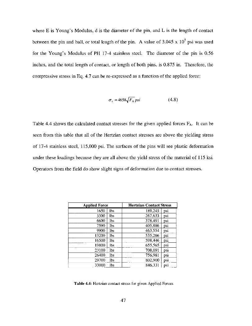
Table 4.4 shows the calculated contact stresses for the given applied forces FA. It can be

seen from this table that all of the Hertzian contact stresses are above the yielding stress

of 17-4 stainless steel, 115,000 psi. The surfaces of the pins will see plastic deformation

under these loadings because they are all above the yield stress of the material of 115 ksi.

Operators from the field do show slight signs of deformation due to contact stresses.

Applied Force I Hertzian Contact Stress1650 lbs 189,245 psi3300 lbs 267,633 psi6600 lbs 378,491 psi7590 lbs 405,886 psi9900 lbs 463,554 psi


Table 4.4: Hertzian contact stress for given Applied Forces

47

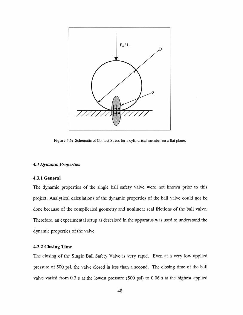
FA/L

Figure 4.6: Schematic of Contact Stress for a cylindrical member on a flat plane.

4.3 Dynamic Properties

4.3.1 General

The dynamic properties of the single ball safety valve were not known prior to this

project. Analytical calculations of the dynamic properties of the ball valve could not be

done because of the complicated geometry and nonlinear seal frictions of the ball valve.

Therefore, an experimental setup as described in the apparatus was used to understand the

dynamic properties of the valve.

4.3.2 Closing Time

The closing of the Single Ball Safety Valve is very rapid. Even at a very low applied

pressure of 500 psi, the valve closed in less than a second. The closing time of the ball

valve varied from 0.3 s at the lowest pressure (500 psi) to 0.06 s at the highest applied

48

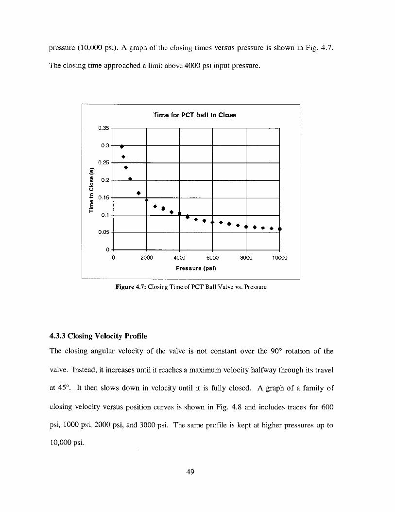
pressure (10,000 psi). A graph of the closing times versus pressure is shown in Fig. 4.7.

The closing time approached a limit above 4000 psi input pressure.

Time for PCT ball to Close

0.35

0.3 -

0.25

0.2 -0

S0.15

0

0.1

0.05-

0-

0 2000 4000 6000 8000 10000

Pressure (psi)

Figure 4.7: Closing Time of PCT Ball Valve vs. Pressure

4.3.3 Closing Velocity Profile

The closing angular velocity of the valve is not constant over the 90 rotation of the

valve. Instead, it increases until it reaches a maximum velocity halfway through its travel

at 45'. It then slows down in velocity until it is fully closed. A graph of a family of

closing velocity versus position curves is shown in Fig. 4.8 and includes traces for 600

psi, 1000 psi, 2000 psi, and 3000 psi. The same profile is kept at higher pressures up to

10,000 psi.

49

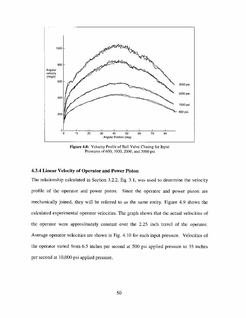
1000

0 10 20 30 40 50 60 70 80


Figure 4.8: Velocity Profile of Ball Valve Closing for InputPressures of 600, 1000, 2000, and 3000 psi

4.3.4 Linear Velocity of Operator and Power Piston

The relationship calculated in Section 3.2.2, Eq. 3.1, was used to determine the velocity

profile of the operator and power piston. Since the operator and power piston are

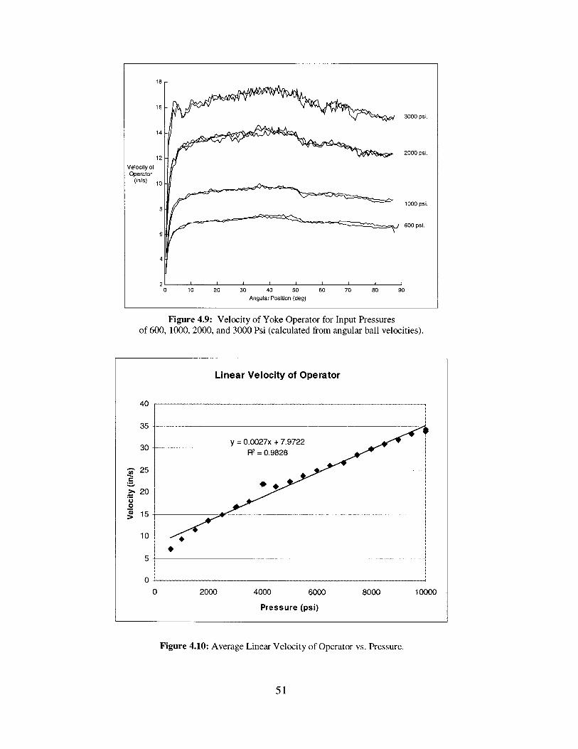
mechanically joined, they will be referred to as the same entity. Figure 4.9 shows the

calculated experimental operator velocities. The graph shows that the actual velocities of

the operator were approximately constant over the 2.25 inch travel of the operator.

Average operator velocities are shown in Fig. 4.10 for each input pressure. Velocities of

the operator varied from 6.5 inches per second at 500 psi applied pressure to 35 inches

per second at 10,000 psi applied pressure.

50

800 -

Angularvelocity(deg/s)

600 -3000 psi.

2000 psi.400 -

1000 psi.

200 600 psi.

18

16

1 6 -3 0 0 0 p s i.

14-

12 -2000 psi.

Velocity ofOperator

(in/s) 10

1000 psi.

600 psi.

6

4,

0 10 20 30 40 50 60 70 80 90Angular Position (deg)

Figure 4.9: Velocity of Yoke Operator for Input Pressuresof 600, 1000, 2000, and 3000 Psi (calculated from angular ball velocities).

Figure 4.10: Average Linear Velocity of Operator vs. Pressure.

51

Linear Velocity of Operator

40

35

y =0.0027x + 7.972230 = R2 0.9828

S25

S20

0

5-

00 2000 4000 6000 8000 10000

Pressure (psi)

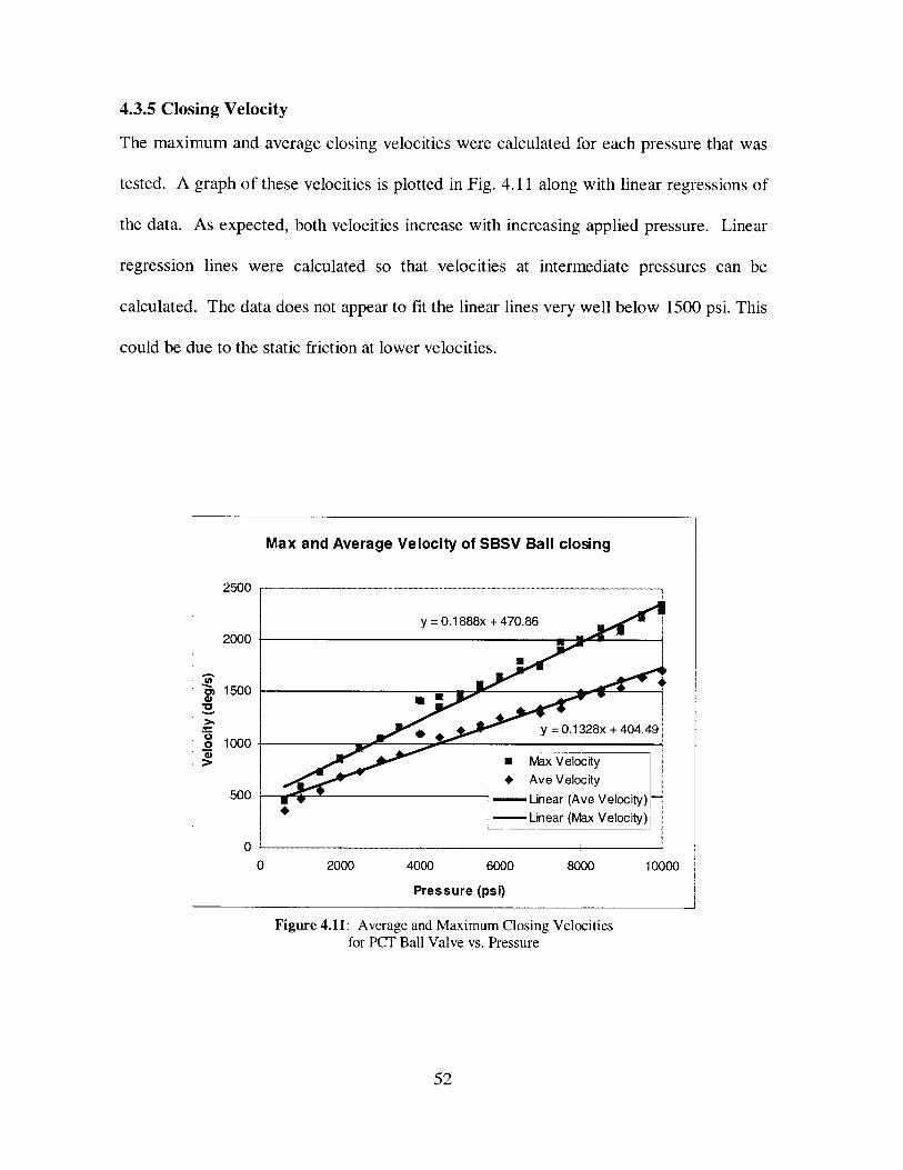
4.3.5 Closing Velocity

The maximum and average closing velocities were calculated for each pressure that was

tested. A graph of these velocities is plotted in Fig. 4.11 along with linear regressions of

the data. As expected, both velocities increase with increasing applied pressure. Linear

regression lines were calculated so that velocities at intermediate pressures can be

calculated. The data does not appear to fit the linear lines very well below 1500 psi. This

could be due to the static friction at lower velocities.

Max and Average Velocity of SBSV Ball closing

2500 ------ -

y =0. 1888x + 470.862000

1500 lie

y .1 328x +404.49o 1000

> Max Velocity* Ave Velocity

500 g--- Linear (Ave Velocity)- Linear (Max Velocity)

00 2000 4000 6000 8000 10000

Pressure (psi)

Figure 4.11: Average and Maximum Closing Velocitiesfor PCT Ball Valve vs. Pressure

52

5 Re-Designed Operator: Lentzerator

5.1 Design Process

Once the efficiency and dynamic properties of the current ball valve assembly were

known, redesigns of the assembly were considered. There were several constraints

imposed on the re-design of the ball valve. Absolute constraints were imposed by the

management at Schlumberger and are as follows [9, 26]:

e Any changes to the ball valve must be compatible with existing tools so thatthe design can be retro-fitted into existing tools.

e Changing the entire seal and valve is too complex of an undertaking for thescope and length of the project.

e The length of the stroke of the piston cannot be changed. Certain toolsincluding the IRDV are limited in the volume of fluid dispensed per stroke,and these values cannot be changed [7].

The design problem was further constrained through self-imposed constraints which were

in place to assure that the design would be easy to implement in current tools, and are as

follows:

e The design should minimize changes to the ball valve. Changing few partswill lead to a more robust system where most of the parts have been proven inthe field. Also, fewer changes means that less parts will have to be replacedwhen the design is retro-fitted into existing tools. This will reduce the totalcosts of implementing the design.

e No moving parts should be added to the ball valve. The ball valve shouldremain simple because the reliability in the harsh downhole environment willdecrease as moving parts are added to the system.

e The overall length and diameter of the tool should not be changed. Addinglength to the ball valve section will increase shipping costs and increase toolstring lengths. The diameter of the ball valve cannot be changed since it mustfit inside of oil well pipes.

53

After considering the many constraints on the re-design of the ball valve and gaining an

understanding of the motion of the linkage using Working Model-3D, the design problem

was reduced to a few options. First, the slot on the ball could be changed so that it had a

different profile. Secondly, the pins on the yoke operator could be changed so that they

had different shapes. A final option included changing both the ball slot and the operator

pin so that an entirely new linkage was designed.

After some investigation into each of these options, it became clear that a change to the

yoke operator would have the most effect for successfully increasing the efficiency of the

linkage. This is because the shape of the operator pin determines the length of the

moment arm of the linkage. Changing the slot of the ball has the effect of varying the

angle that operator pin makes with the ball. Adding a profile to the ball slot can have the

effect of changing the velocity and acceleration of the ball, but will not have a significant

impact on the moment arm of the linkage. Several other ideas were considered that

required changes to both the ball slot and the operator pin, however, when loading and

shear stresses were calculated, none were strong enough to withstand the high closing

forces.

It turns out that the current design is very good and is nearly the best that can be done,

except for the fact that the designers did not consider how the moment arm would change

over the length of the stroke [26]. At the time of the design, Schlumberger was not

concerned with either wireline cutting or high closing forces. The primary design

parameter was the opening force, which is responsible for overcoming static seal friction

54

and opening the valve [26]. It was only recently that sealing with a high differential

pressure and cutting wireline monocable were added to the design requirements [9].

Once the other two options were ruled out, modifications were made to the pin geometry

of the yoke operator, creating a cam profile so that more torque is available for a given

applied force. The complex nature of the rotating ball slot and linearly moving operator

caused this redesign to be non-intuitive, so no one had previously considered making this

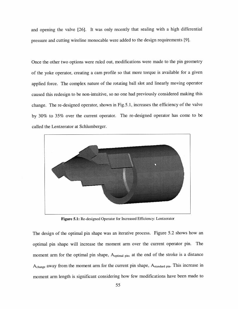
change. The re-designed operator, shown in Fig.5.1, increases the efficiency of the valve

by 30% to 35% over the current operator. The re-designed operator has come to be

called the Lentzerator at Schlumberger.

Figure 5.1: Re-designed Operator for Increased Efficiency: Lentzerator

The design of the optimal pin shape was an iterative process. Figure 5.2 shows how an

optimal pin shape will increase the moment arm over the current operator pin. The

moment arm for the optimal pin shape, Aoptimai pin, at the end of the stroke is a distance

Achange away from the moment arm for the current pin shape, Astandad pin. This increase in

moment arm length is significant considering how few modifications have been made to

55

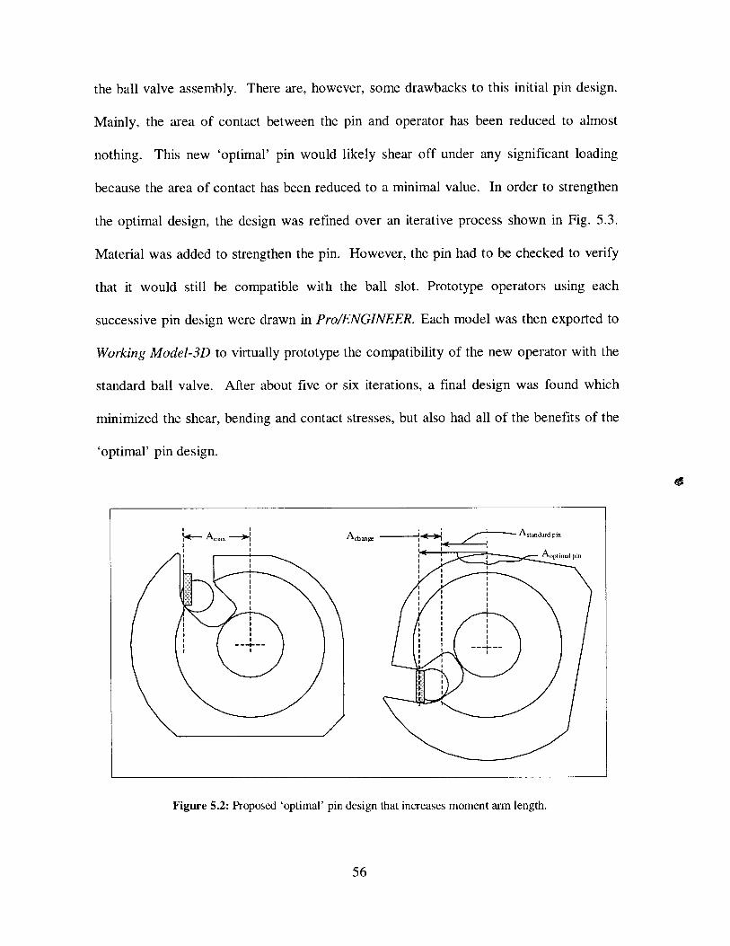
the ball valve assembly. There are, however, some drawbacks to this initial pin design.

Mainly, the area of contact between the pin and operator has been reduced to almost

nothing. This new 'optimal' pin would likely shear off under any significant loading

because the area of contact has been reduced to a minimal value. In order to strengthen

the optimal design, the design was refined over an iterative process shown in Fig. 5.3.

Material was added to strengthen the pin. However, the pin had to be checked to verify

that it would still be compatible with the ball slot. Prototype operators using each

successive pin design were drawn in Pro/ENGINEER. Each model was then exported to

Working Model-3D to virtually prototype the compatibility of the new operator with the

standard ball valve. After about five or six iterations, a final design was found which

minimized the shear, bending and contact stresses, but also had all of the benefits of the

'optimal' pin design.

I*- Amax AAchangAsaniard pin

A.ptimoa pin

Figure 5.2: Proposed 'optimal' pin design that increases moment arm length.

56

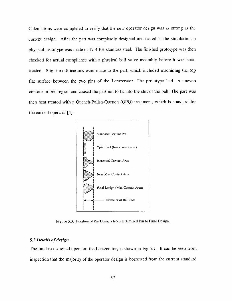
Calculations were completed to verify that the new operator design was as strong as the

current design. After the part was completely designed and tested in the simulation, a

physical prototype was made of 17-4 PH stainless steel. The finished prototype was then

checked for actual compliance with a physical ball valve assembly before it was heat-

treated. Slight modifications were made to the part, which included machining the top

flat surface between the two pins of the Lentzerator. The prototype had an uneven

contour in this region and caused the part not to fit into the slot of the ball. The part was

then heat treated with a Quench-Polish-Quench (QPQ) treatment, which is standard for

the current operator [4].

Q Standard Circular Pin

Optimized (low contact area

Increased Contact Area

Near Max Contact Area

Final Design (Max Contact

Diameter of Ball Slot

Area)

Figure 5.3: Iteration of Pin Designs from Optimized Pin to Final Design.

5.2 Details of design

The final re-designed operator, the Lentzerator, is shown in Fig.5. 1. It can be seen from

inspection that the majority of the operator design is borrowed from the current standard

57

)

yoke operator, shown in Fig. 2.3. This is necessary to keep it compatible with the

existing power piston and ball slot. Essentially, the only change was made to the

operator pins. The pins have been changed so that the point of contact between the

operator and the ball is a maximum distance from the center of rotation of the ball. By

changing the contact point, the effective moment arm that actuates the ball has been

increased.

Figure 5.4 shows the contact point of the new pin compared to the standard pin for three

angular positions. At 0' of rotation, both pins make contact with the ball in

approximately the same place. By the time the ball has rotated halfway closed 450, the

contact point has moved to the center of the circular pin on the standard operator, but the

contact point is still in the same general area on the Lentzerator. The gains in efficiency

become obvious when the valve is examined at the 700 point. Both cutting of wireline

monocable and sealing against high differential pressure occur at approximately 70'

closed. The contact point of the standard pin has now moved to the inside surface of the

circle, while the re-designed pin still makes contact at the same general point as in the

450 case.

The details of the re-designed pin are shown in Fig. 5.5. The pin has the same bounding

characteristics as the current pin design. The height of the pin remains the same as the

diameter of the current pin so that hold open conditions remain the same. Also, the front

edge of the pin remains the same distance from the end of the operator so that when the

ball is in the closed position, the operator mandrel piston will be in the same position as

58

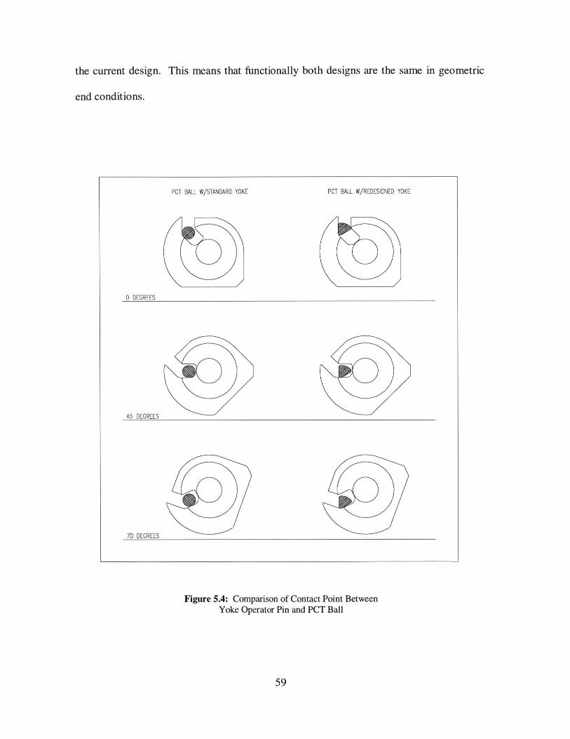
the current design. This means that functionally both designs are the same in geometric

end conditions.

Figure 5.4: Comparison of Contact Point BetweenYoke Operator Pin and PCT Ball

59

PCT BALL W/REDESIGNED YOKEPCT BALL W/STANDARD YOKE

0 DEGREES

45 DEGREES

70 DEGREES

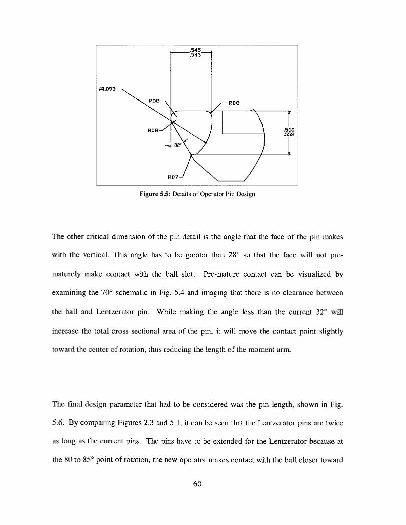
R07

Figure 5.5: Details of Operator Pin Design

The other critical dimension of the pin detail is the angle that the face of the pin makes

with the vertical. This angle has to be greater than 280 so that the face will not pre-

maturely make contact with the ball slot. Pre-mature contact can be visualized by

examining the 70' schematic in Fig. 5.4 and imaging that there is no clearance between

the ball and Lentzerator pin. While making the angle less than the current 320 will

increase the total cross sectional area of the pin, it will move the contact point slightly

toward the center of rotation, thus reducing the length of the moment arm.

The final design parameter that had to be considered was the pin length, shown in Fig.

5.6. By comparing Figures 2.3 and 5.1, it can be seen that the Lentzerator pins are twice

as long as the current pins. The pins have to be extended for the Lentzerator because at

the 80 to 850 point of rotation, the new operator makes contact with the ball closer toward

60

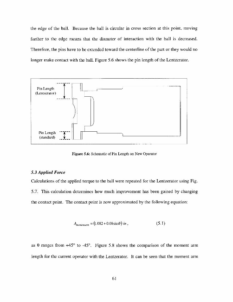
the edge of the ball. Because the ball is circular in cross section at this point, moving

further to the edge means that the diameter of interaction with the ball is decreased.

Therefore, the pins have to be extended toward the centerline of the part or they would no

longer make contact with the ball. Figure 5.6 shows the pin length of the Lentzerator.

Pin Length(Lentzerator)

Pin Length ~~~-~~(standard) __

Figure 5.6: Schematic of Pin Length on New Operator

5.3 Applied Force

Calculations of the applied torque to the ball were repeated for the Lentzerator using Fig.

5.7. This calculation determines how much improvement has been gained by changing

the contact point. The contact point is now approximated by the following equation:

Anomentarm = (1.082+0.08 sin 6) in, (5.1)

as 0 ranges from +450 to -45'. Figure 5.8 shows the comparison of the moment arm

length for the current operator with the Lentzerator. It can be seen that the moment arm

61

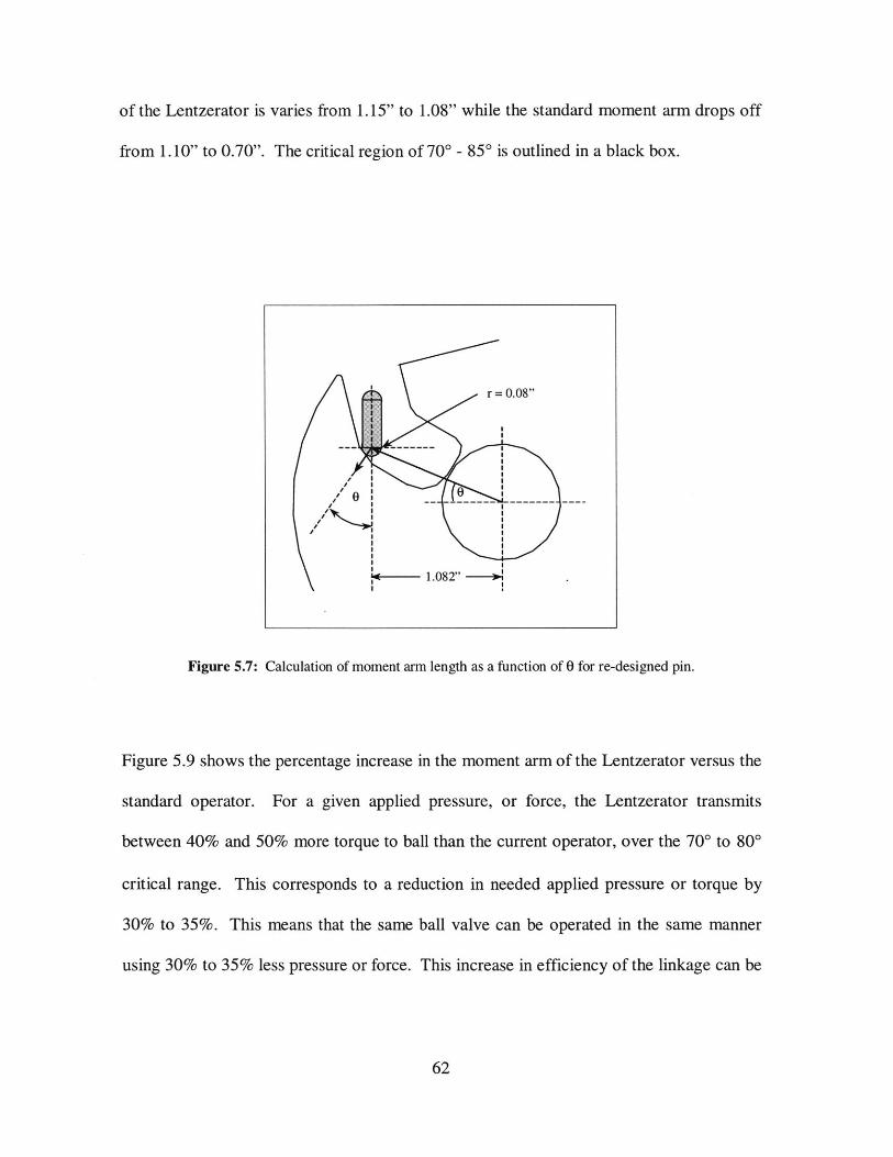
of the Lentzerator is varies from 1.15" to 1.08" while the standard moment arm drops off

from 1.10" to 0.70". The critical region of 700 - 850 is outlined in a black box.

Figure 5.7: Calculation of moment arm length as a function of 0 for re-designed pin.

Figure 5.9 shows the percentage increase in the moment arm of the Lentzerator versus the

standard operator. For a given applied pressure, or force, the Lentzerator transmits

between 40% and 50% more torque to ball than the current operator, over the 700 to 800

critical range. This corresponds to a reduction in needed applied pressure or torque by

30% to 35%. This means that the same ball valve can be operated in the same manner

using 30% to 35% less pressure or force. This increase in efficiency of the linkage can be

62

used to reduce operating pressure or force requirements, or to reduce the size of nitrogen

and Belleville spring chambers.

For the input pressures over the range of 500 psi to 10,000 psi, Table 5.1 summarizes the

applied force. It is important to realize that to get the same closing pressure, the applied

pressure for the Lentzerator is less than the standard operator by 33%.

as Function of Position

1.30

1.20

1.10

1.00

0.90

0.80

0.70

0.60

0.50

0.40

0.30

0.20

0.10

0.00758085900 5 10152025303540455055606570


Figure 5.8: Moment Arm Length vs. Angular Positionfor Current Operator and Lentzerator.

63

0

0c.

0

CL0(U

E

0Q

o0

""U

a,-

cc

.g0

0

C.

-

Re-Designed

---- Current

Moment Arm Length

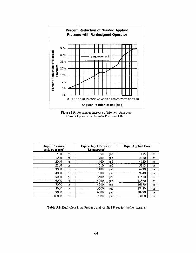
Percent Reduction of Needed AppliedPressure with Re-designed Operator

35%-_ T ___ ------

30% -- % Irrprovementz

4- 25%-0

10%

0 5 10 15 20 25 30 35 40 45 50 55 60 65 70 75 80 85 90


Figure 5.9: Percentage Increase of Moment Arm overCurrent Operator vs. Angular Position of Ball.

Input Pressure Equiv. Input Pressure Eqiv. Applied Force(std. operator) (Lentzerator)

500 psi 350 psi 1155 lbs1000 psi 700 psi 2310 lbs2000 psi 1400 psi 4620 lbs2300 psi 1610 psi 5313 lbs3000 psi 2100 psi 6930 lbs4000 psi 2800 psi 9240 lbs5000 psi 3500 psi 11550 lbs6000 psi 4200 psi 13860 lbs7000 psi 4900 psi 16170 lbs8000 psi 5600 psi 18480 lbs9000 psi 6300 psi 20790 lbs

10000 psi 7000 psi 23100 lbs

Table 5.1: Equivalent Input Pressure and Applied Force for the Lentzerator

64

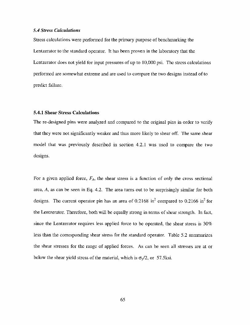
5.4 Stress Calculations

Stress calculations were performed for the primary purpose of benchmarking the

Lentzerator to the standard operator. It has been proven in the laboratory that the

Lentzerator does not yield for input pressures of up to 10,000 psi. The stress calculations

performed are somewhat extreme and are used to compare the two designs instead of to

predict failure.

5.4.1 Shear Stress Calculations

The re-designed pins were analyzed and compared to the original pins in order to verify

that they were not significantly weaker and thus more likely to shear off. The same shear

model that was previously described in section 4.2.1 was used to compare the two

designs.

For a given applied force, FA, the shear stress is a function of only the cross sectional

area, A, as can be seen in Eq. 4.2. The area turns out to be surprisingly similar for both

designs. The current operator pin has an area of 0.2168 in2 compared to 0.2166 in 2 for

the Lentzerator. Therefore, both will be equally strong in terms of shear strength. In fact,

since the Lentzerator requires less applied force to be operated, the shear stress is 30%

less than the corresponding shear stress for the standard operator. Table 5.2 summarizes

the shear stresses for the range of applied forces. As can be seen all stresses are at or

below the shear yield stress of the material, which is yy/2, or 57.5ksi.

65

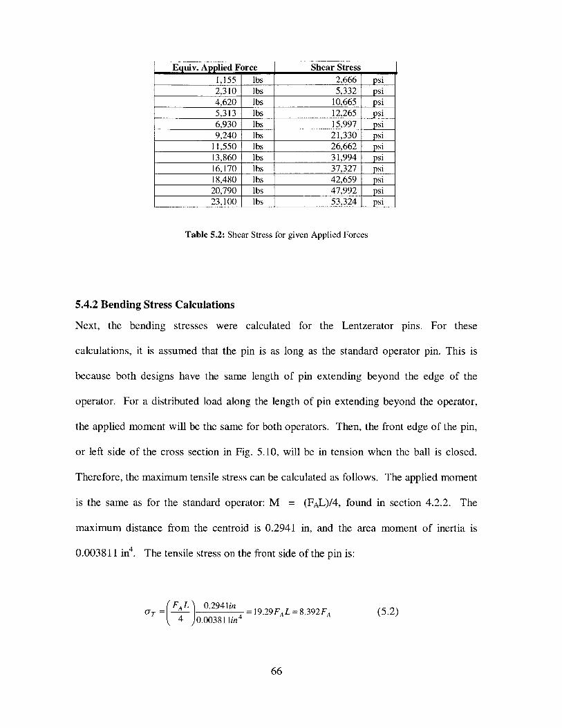
Equiv. Applied Force Shear Stress

1,155 lbs 2,666 psi2,310 lbs 5,332 psi4,620 lbs 10,665 psi5,313 lbs 12,265 psi6,930 lbs 15,997 psi9,240 lbs 21,330 psi

11,550 lbs 26,662 psi13,860 lbs 31,994 psi16,170 lbs 37,327 psi18,480 lbs 42,659 psi20,790 lbs 47,992 psi23,100 lbs 53,324 psi

Table 5.2: Shear Stress for given Applied Forces

5.4.2 Bending Stress Calculations

Next, the bending stresses were calculated for the Lentzerator pins. For these

calculations, it is assumed that the pin is as long as the standard operator pin. This is

because both designs have the same length of pin extending beyond the edge of the

operator. For a distributed load along the length of pin extending beyond the operator,

the applied moment will be the same for both operators. Then, the front edge of the pin,

or left side of the cross section in Fig. 5.10, will be in tension when the ball is closed.

Therefore, the maximum tensile stress can be calculated as follows. The applied moment

is the same as for the standard operator: M = (FAL)/4, found in section 4.2.2. The

maximum distance from the centroid is 0.2941 in, and the area moment of inertia is

0.003811 in4 . The tensile stress on the front side of the pin is:

(FL~0.2941in07r =FAL 0 4 = 19.29FAL = 8.3 9 2 FA (5.2)

4 0.003811in4

66

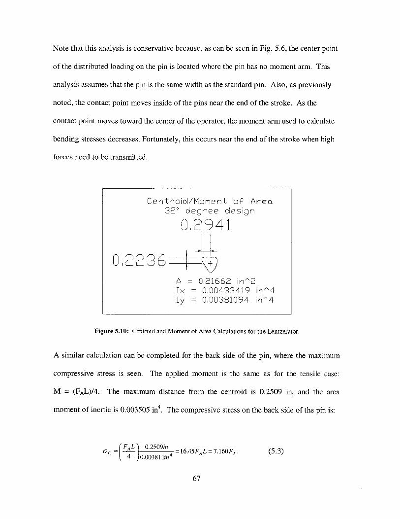
Note that this analysis is conservative because, as can be seen in Fig. 5.6, the center point

of the distributed loading on the pin is located where the pin has no moment arm. This

analysis assumes that the pin is the same width as the standard pin. Also, as previously

noted, the contact point moves inside of the pins near the end of the stroke. As the

contact point moves toward the center of the operator, the moment arm used to calculate

bending stresses decreases. Fortunately, this occurs near the end of the stroke when high

forces need to be transmitted.

Figure 5.10: Centroid and Moment of Area Calculations for the Lentzerator.

A similar calculation can be completed for the back side of the pin, where the maximum

compressive stress is seen. The applied moment is the same as for the tensile case:

M = (FAL)/4. The maximum distance from the centroid is 0.2509 in, and the area

moment of inertia is 0.003505 in4. The compressive stress on the back side of the pin is:

Oc= FA L 0.2509in =16.45FAL = 7.160FA.4 0.003811in 4

(5.3)

67

Centroid/Moment o-f Areoa32* degree cesign

02941

02236A 0.21662 in^2Ix 0.00433419 in^<4Iy 0.00381094 in^4

For an applied force on the front side of the pin, the Lentzerator will see a slightly higher

tensile stress than the standard operator, but will see a slightly lower compressive stress

on the back side of the pin. However, since the Lentzerator requires less applied force to

be operated, the bending stress is on the order of 30% less than the corresponding

bending stress for the standard operator. Table 5.3 shows the calculated bending stresses

for the Lentzerator, using Eqs. 5.2 and 5.3.

Equiv. Applied Force Tensile Stress Compressive Stress1,155 lbs 9,693 psi 8,269 psi2,310 lbs 19,387 psi 16,539 psi4,620 lbs 38,773 psi 33,078 psi5,313 lbs 44,589 psi 38,039 psi6,930 lbs 58,160 psi 49,617 psi9,240 lbs 77,547 psi 66,156 psi

11,550 lbs 96,933 psi 82,695 psi13,860 lbs 116,320 psi 99,233 psi16,170 lbs 135,707 psi 115,772 psi18,480 lbs 155,093 psi 132,311 psi20,790 lbs 174,480 psi 148,850 psi23,100 lbs 193,867 psi 165,389 psi

Table 5.3: Bending Stresses for given Applied Forces

5.4.3 Contact Stress Calculations

Hertzian contact stresses were calculated for the contact of the Lentzerator pins on the

ball using the previously described analysis in section 4.2.3. A value of 3.045 x 107 psi

was used for the Young's Modulus of PH 17-4 stainless steel. The diameter of the

contact cylinder is now 0.16 inches, and the length of contact, or length of the pins, is

now twice as long, 1.75 in. The compressive stress can be re-expressed as a function of

the applied force:

68

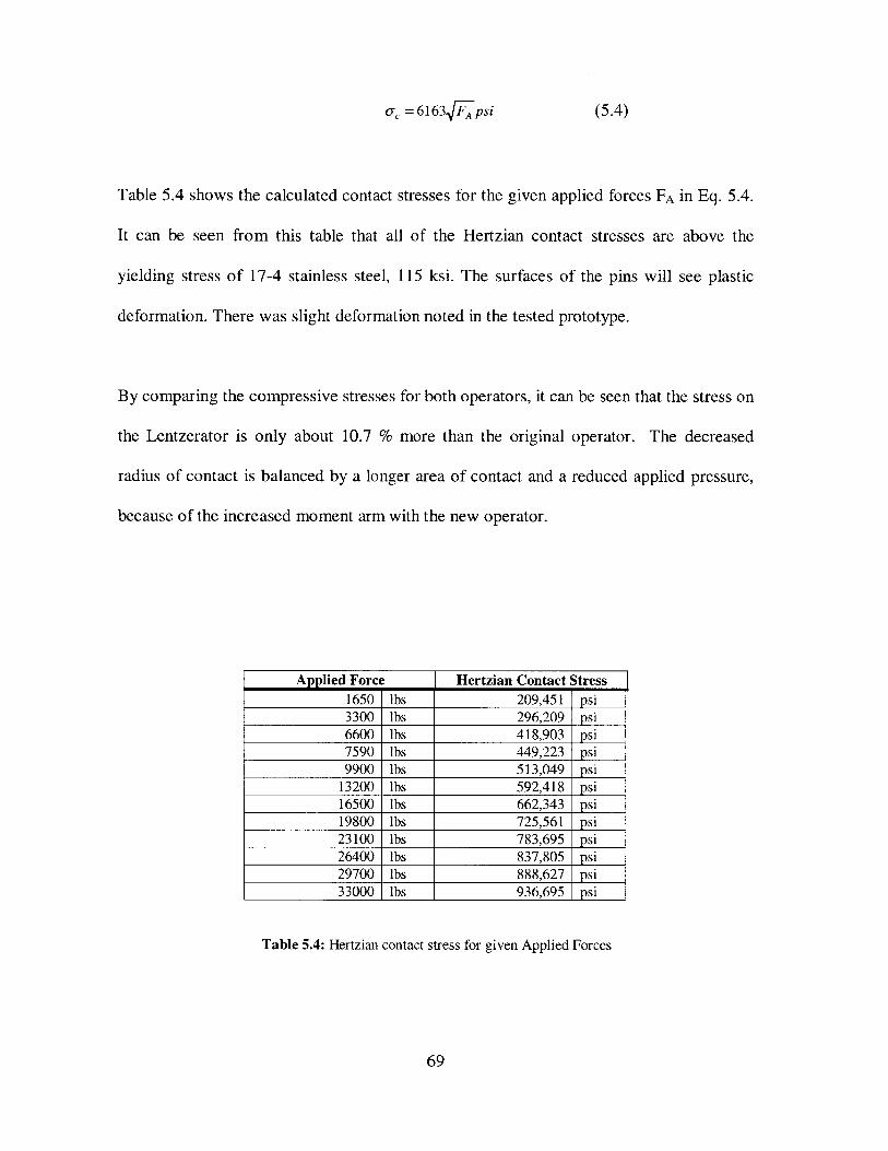
c = 6163VFApsi

Table 5.4 shows the calculated contact stresses for the given applied forces FA in Eq. 5.4.

It can be seen from this table that all of the Hertzian contact stresses are above the

yielding stress of 17-4 stainless steel, 115 ksi. The surfaces of the pins will see plastic

deformation. There was slight deformation noted in the tested prototype.

By comparing the compressive stresses for both operators, it can be seen that the stress on

the Lentzerator is only about 10.7 % more than the original operator. The decreased

radius of contact is balanced by a longer area of contact and a reduced applied pressure,

because of the increased moment arm with the new operator.

Applied Force Hertzian Contact Stress1650 lbs 209,451 psi3300 lbs 296,209 psi6600 lbs 418,903 psi7590 lbs 449,223 psi9900 lbs 513,049 psi


Table 5.4: Hertzian contact stress for given Applied Forces

69

(5.4)

5.5 Dynamic Properties

Once the applied force was calculated, the velocity profile of the Lentzerator was

investigated. The velocity profile was first predicted using the simulation in Working

Model-3D, and then was measured in the laboratory using the same encoder and

accumulator set up as was used for the standard operator.

5.5.1 Predicted Closing Velocity Profile

The velocity profile was predicted with the simulation in Working Model-3D by applying

a constant velocity to the operator and measuring the output angular velocity of the ball.

A screen shot from Working Model-3D is shown in Fig. 5.11. It was assumed that the

operator had the same motion for the new operator as it did for the standard operator.

Values for the linear velocity of the Lentzerator were taken from the previous

experimental data. Figure 5.12 shows the predicted velocity profiles for inputs of 1000,

2000, and 3000 psi.

70

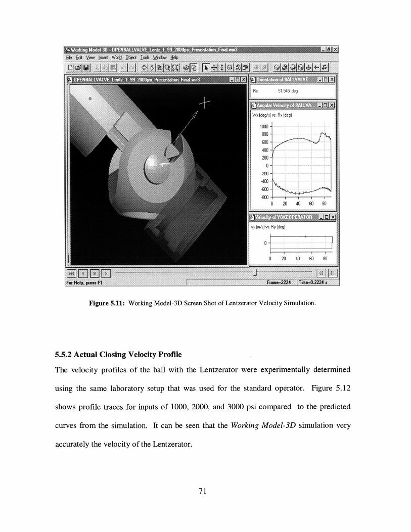
F A ---------- --- --- - .. ....

Figure 5.11: Working Model-3D Screen Shot of Lentzerator Velocity Simulation.

5.5.2 Actual Closing Velocity Profile

The velocity profiles of the ball with the Lentzerator were experimentally determined

using the same laboratory setup that was used for the standard operator. Figure 5.12

shows profile traces for inputs of 1000, 2000, and 3000 psi compared to the predicted

curves from the simulation. It can be seen that the Working Model-3D simulation very

accurately the velocity of the Lentzerator.

71

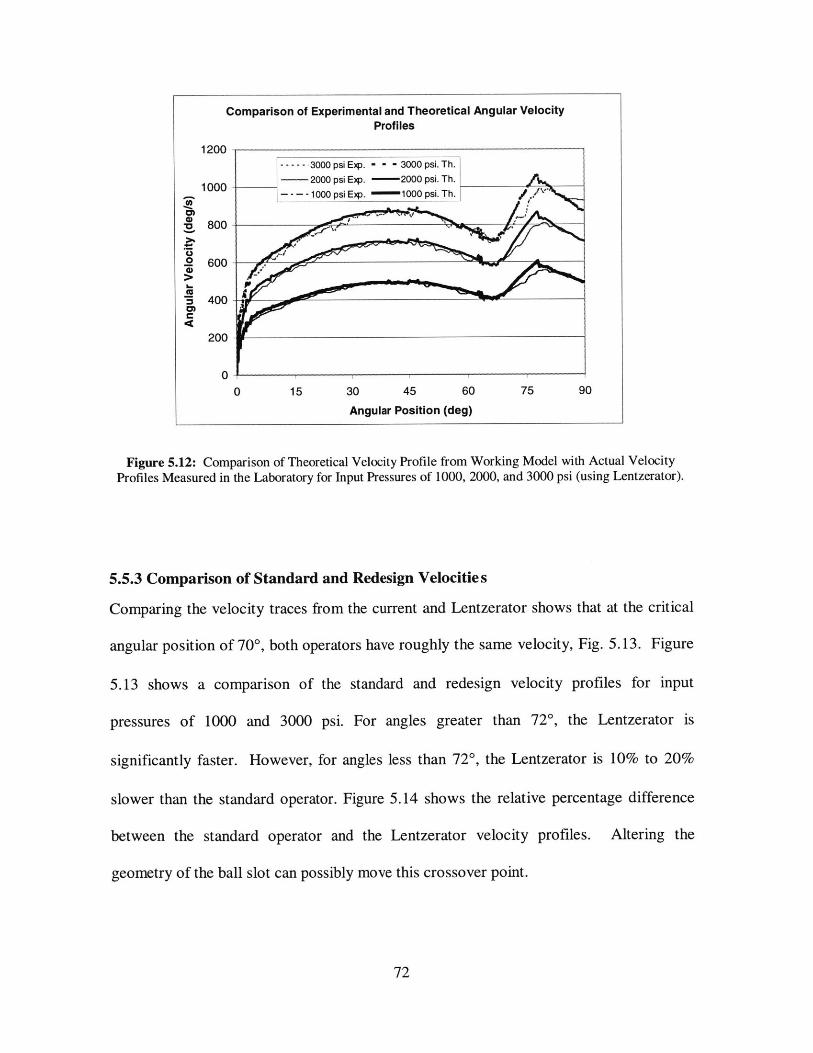
Figure 5.12: Comparison of Theoretical Velocity Profile from Working Model with Actual VelocityProfiles Measured in the Laboratory for Input Pressures of 1000, 2000, and 3000 psi (using Lentzerator).

5.5.3 Comparison of Standard and Redesign Velocities

Comparing the velocity traces from the current and Lentzerator shows that at the critical

angular position of 700, both operators have roughly the same velocity, Fig. 5.13. Figure

5.13 shows a comparison of the standard and redesign velocity profiles for input

pressures of 1000 and 3000 psi. For angles greater than 720, the Lentzerator is

significantly faster. However, for angles less than 720, the Lentzerator is 10% to 20%

slower than the standard operator. Figure 5.14 shows the relative percentage difference

between the standard operator and the Lentzerator velocity profiles. Altering the

geometry of the ball slot can possibly move this crossover point.

72

Comparison of Experimental and Theoretical Angular VelocityProfiles

1200- -- --- 3000 psi Exp. - - - 3000 psi. Th.

1000 ---- 2000 psi Ep. -2000 psi. Th.----1000 psi Exp. - 1000 psi. Th.

800

00 15 30 45 60 75 90


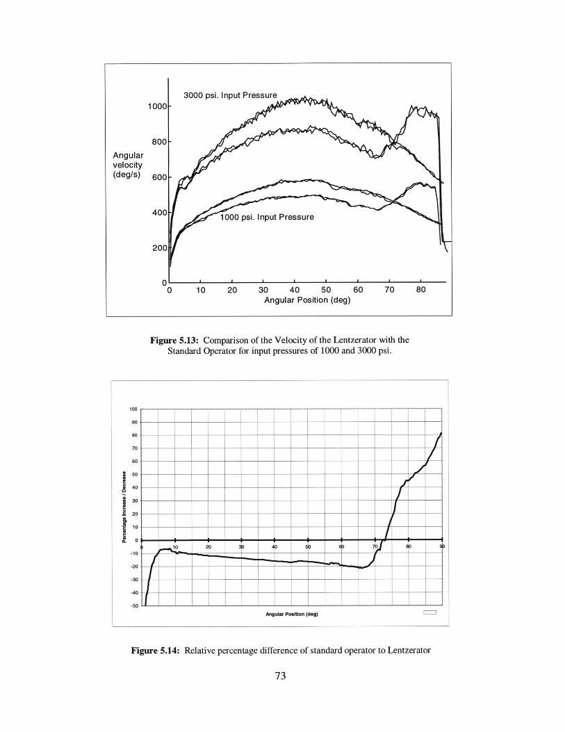
Figure 5.13: Comparison of the Velocity of the Lentzerator with theStandard Operator for input pressures of 1000 and 3000 psi.

Angular Position (dog)

Figure 5.14: Relative percentage difference of standard operator to Lentzerator

73

a

&a

a.

6 Testing of Lentzerator Prototype

Several tests were conducted using the Lentzerator prototype to confirm the predicted

increases in efficiency. These tests are described in more detail in sections 3.1.3 and

3.1.4. Cycling tests were conducted to check for any abnormal wear of the operator and

cutting tests were conducted to verify the increase in applied torque.

6.1 Cycling Tests

The operator prototype was cycled for a total of 106 strokes at pressures ranging from

500 psi to 10,000 psi. Of these 106 strokes, twenty were cutting tests that put abnormally

high impact loads on the contact surface. The operator showed slight wear after the first

30 cycles on the part of the pin length that extended inside the standard operator pins.

Since the ball was old and fairly worn by the standard operator, there were grooves in the

ball slots where the operator pins had contacted the ball. So, when the Lentzerator

moved in the slot with its pins that were twice as wide as the standard operator, half of

the pin was riding on the un-worn part of the ball slot. Because of this uneven contact on

the pin of the Lentzerator, unnatural wear was induced. If the Lentzerator is used with a

new ball, this uneven wear should not be a problem.

6.2 Cutting Tests

6.2.1 General Procedure

Cutting tests were used as a benchmark for comparing the two operators. Although

cutting wireline monocable is not the most repeatable method for testing a prototype

against a baseline, wireline cutting is one of the two applications of the Lentzerator. By

benchmarking the operator with wireline cutting, it was possible to accomplish two

74

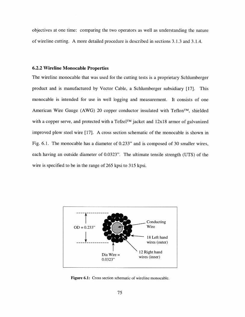
objectives at one time: comparing the two operators as well as understanding the nature

of wireline cutting. A more detailed procedure is described in sections 3.1.3 and 3.1.4.

6.2.2 Wireline Monocable Properties

The wireline monocable that was used for the cutting tests is a proprietary Schlumberger

product and is manufactured by Vector Cable, a Schlumberger subsidiary [17]. This

monocable is intended for use in well logging and measurement. It consists of one

American Wire Gauge (AWG) 20 copper conductor insulated with TeflonTM, shielded

with a copper serve, and protected with a TefzelTM jacket and 12x18 armor of galvanized

improved plow steel wire [17]. A cross section schematic of the monocable is shown in

Fig. 6.1. The monocable has a diameter of 0.233" and is composed of 30 smaller wires,

each having an outside diameter of 0.0323". The ultimate tensile strength (UTS) of the

wire is specified to be in the range of 265 kpsi to 315 kpsi.

OD = 0.233"

--------------

Dia Wire0.0323"

ConductingWire

18 Left handwires (outer)

12 Right handwires (inner)

Figure 6.1: Cross section schematic of wireline monocable.

75

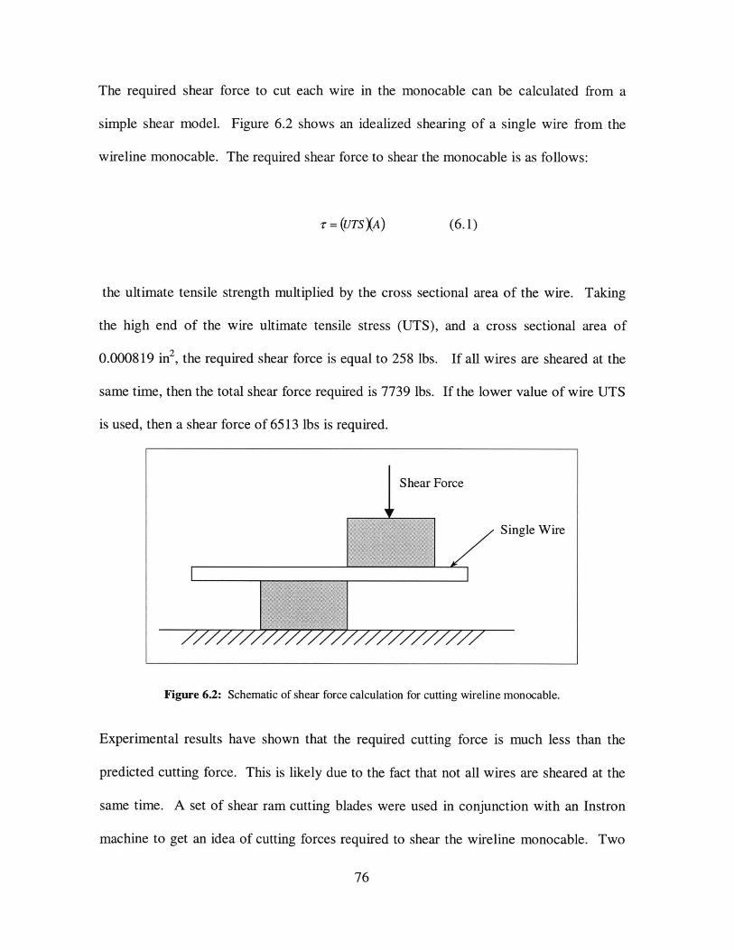
The required shear force to cut each wire in the monocable can be calculated from a

simple shear model. Figure 6.2 shows an idealized shearing of a single wire from the

wireline monocable. The required shear force to shear the monocable is as follows:

r = (UTSXA) (6.1)

the ultimate tensile strength multiplied by the cross sectional area of the wire. Taking

the high end of the wire ultimate tensile stress (UTS), and a cross sectional area of

0.000819 in2, the required shear force is equal to 258 lbs. If all wires are sheared at the

same time, then the total shear force required is 7739 lbs. If the lower value of wire UTS

is used, then a shear force of 6513 lbs is required.

Shear Force

Single Wire

Figure 6.2: Schematic of shear force calculation for cutting wireline monocable.

Experimental results have shown that the required cutting force is much less than the

predicted cutting force. This is likely due to the fact that not all wires are sheared at the

same time. A set of shear ram cutting blades were used in conjunction with an Instron

machine to get an idea of cutting forces required to shear the wireline monocable. Two

76

tests were run with no tension on the wire. Twenty-seven of 30 wires were cut, requiring

an average shear force of 2475 lbs.

This shear force corresponds to the force applied by the edge of the cutting ball when

wireline is cut using the Single Ball Safety Valve (SBSV). The cutting edge force can be

calculated from the applied force by knowing that the cutting edge has a moment arm of

exactly 2.0", because the ball has a diameter of 4". So, for a given input torque equal to

the applied force, FA, times the moment arm, the cutting edge force can be calculated.

The length of the moment arm can be calculated for the standard operator and the

Lentzerator at the 700 cutting angle. The standard operator has a moment arm of 0.730"

and the Lentzerator has a moment arm of 1.084". The average force at cut edge was

calculated for 15 static wireline cuts and the average was 2760 lbs. Again, this value is

much less than the theoretical value, but is quite close to the value from the Instron shear

ram tests.

6.2.3 Summarized Cutting Results

The results of the cutting tests were as good or better than expected. The Lentzerator cut

at an average input pressure that was 33% less than the original operator. This

corresponds to an increase in moment arm length of 49%, which was on the high end of

the predicted improvement. Detailed static results from the static cutting tests are

included in Appendix A. 1. The average pressure needed to cut with the standard operator

was 2305 psi, but only 1551 psi for the Lentzerator.

77

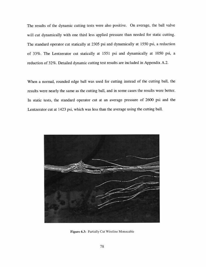
The results of the dynamic cutting tests were also positive. On average, the ball valve

will cut dynamically with one third less applied pressure than needed for static cutting.

The standard operator cut statically at 2305 psi and dynamically at 1550 psi, a reduction

of 33%. The Lentzerator cut statically at 1551 psi and dynamically at 1050 psi, a

reduction of 32%. Detailed dynamic cutting test results are included in Appendix A.2.

When a normal, rounded edge ball was used for cutting instead of the cutting ball, the

results were nearly the same as the cutting ball, and in some cases the results were better.

In static tests, the standard operator cut at an average pressure of 2600 psi and the

Lentzerator cut at 1423 psi, which was less than the average using the cutting ball.

Figure 6.3: Partially Cut Wireline Monocable

78

Dynamic cutting tests using standard seal retainer and standard ball valve were

unsuccessful for both of the operators, Fig. 6.3. Only two tests were run because the seal

retainer was destroyed from the test and had to be scrapped. The redesign was able to cut

through three more wires (21/30) than the standard operator was (24/30). Table 6.1

summarizes the cutting test results.

Test Description (num. of tests in braces) Standard LentzeratorOperator

Static cutting of wireline (cut ball & cut sleeve) {9} 2305 psi 1551 psiStatic cutting of wireline (std ball & cut sleeve) {61 2600 psi 1423 psi

Dynamic cutting of wireline (all tests) {6} 1550 psi 1050 psi

Dynamic cutting of wireline (std ball & std sleeve) - 5000psi {2} 70% cut 80% cut

Table 6.1: Summary of Cutting Tests

79

7 Conclusions and Recommendations

7.1 Conclusions

The goal of this thesis was to gain an understanding of the ball valve in use by

Schlumberger in its downhole oil well tools and use this understanding to design

improvements to the valve that increase the performance of the valve. These goals were

successfully accomplished and this thesis presents the design of the Lentzerator, which

will operate with 30% - 35% less applied pressure than the current yoke operator. Tests

were conducted in the laboratory to confirm these performance gains.

Prior to the research that was conducted for this thesis, little was known about the

operation of this ball valve. Most of what was 'known' about its operation was either

hearsay or guesses. An experimental setup was created in the laboratory to measure the

dynamic properties of the valve such as closing times and closing velocity curves. The

valve was then modeled on the computer using Working Model-3D simulation software.

Once the computer model accurately reflected the laboratory data, new designs could be

prototyped virtually using the simulation software. After several design iterations on the

computer, the final design was physically prototyped so that it could be tested in the

laboratory set up. The results from the laboratory tests with the physical prototype were

almost identical to the predicted results from the simulation software, thus confirming the

validity of using this software as a design tool. Now, other parts and tools can be reliably

designed in a similar fashion.

80

The results from the study of the current ball valve showed that there was room to

improve the valve. The moment arm that actuates the ball valve decreases by 55% as the

ball goes from the open to the closed position. This is particularly troubling because a

shorter moment arm means that less force is applied to the valve for a given input

pressure force. Also, it is desired to have a maximum, not a minimum application of

force at the end of the ball stroke because this is where closing forces needed for sealing

and wireline cutting are the highest.

The current ball valve closes very rapidly, with closing times that range from 0.06 to 0.30

seconds and closing angular velocities as high as 2300 degrees per second. The velocity

profile over the closing is negative parabolic in shape, reaching a maximum velocity in

the middle and tapering off at the beginning and end. A reduction in velocity at the end

of the stroke means that dynamic impact forces will be less than with a higher velocity.

The operator was redesigned to improve these shortcomings of the ball valve linkage.

The Lentzerator was designed to increase the length of the moment arm that acts on the

ball valve. Also, the velocity in the critical range of 700 - 85' closed is as high or higher

than the current operator is in the same region. Cutting tests were conducted to verify that

the Lentzerator increased applied torque by 40% to 50% and reduced needed pressure by

30% to 35%, which was predicted. This allows the ball valve to be operated with one

third less applied pressure, increasing the performance of the valve, and reducing the

sizes of nitrogen and belleville spring chambers for some tools. The velocity profile was

also confirmed to be approximately the same as current velocity profile at the cutting

81

angle of 70'. Since the redesign was both innovative and cost saving, a patent was

applied for to prevent competitors from using the design.

Finally, cutting of wireline monocable was investigated. A specially designed cutting

valve consisting of a cutting sleeve and a cutting ball was designed and tested. Another

Schlumberger engineer completed the design work for the cutting valve, but testing of the

valve was conducted as a part of this thesis [18]. For the 0.232" outer diameter wireline

monocable used, a theoretical shear force of about 7000 lbs was calculated. However, an

overall average cutting force of 2760 lbs was measured in the laboratory. This implies

that not all of the wires are sheared at the same time as the model assumes. When

dynamic impact loading is introduced by having the valve close rapidly on the wireline

monocable, the necessary cutting forces decrease significantly. Cutting forces decreased

by an average of 32% for both the standard operator and the Lentzerator when dynamic

tests were run versus static tests. Lastly, cutting tests were run using a combination of the

standard ball with the cutting sleeve. These tests showed that the standard ball is as

effective in wireline monocable cutting as the special cutting ball.

In conclusion, this thesis includes basic research about this valve that was instrumental in

redesigning of the ball valve linkage. When possible, dynamic cutting of wireline

monocable should be implemented because it is 32% more efficient than static cutting.

Working Model-3D can be reliably used as a design tool to help understand complicated

dynamic systems and design improvements of them. Finally, the Lentzerator was

confirmed to improve performance of the ball valve by an average of 33%.

82

7.2 Recommendations for Future Work

The results of this thesis open many doors for future work. First, since the basic dynamic

properties of the valve are now known, dependable virtual simulations of the valve

motion can be created in Working Model-3D. Also, if gauges and other instrumentation

need to be interfaced with the ball valve assembly, the time scale of interaction is now

known, so properly suited gauges can be used. It is also possible to change the ball slot to

make significant improvements in the closing velocity profile. Changes can be made to

the solid model in Pro/ENGINEER and exported to Working Mode-3D to determine their

effects upon the actual velocity profile without having to run time consuming and

expensive laboratory experiments.

The pin shape of the Lentzerator can be applied to the smaller 3" and larger 7" lines of

tools. Similar performance gains should be possible in these families of tools. The

application of the pin shape to the MFE line of ball valves should also be investigated.

Tests can be conducted using either field tests or flow loop laboratory setups to reduce

the operating pressure requirements for valves closing against a differential pressure. In

other tools, Belleville springs may be reduced in length, and nitrogen chambers may also

be able to be shortened.

Finally, when a normal, rounded edge ball was used for cutting instead of the cutting ball,

the results were essentially the same. These results are intriguing because they imply that

it may be possible to incorporate a Viton or Teflon seal into the cutting sleeve, or

alternately, a cutting edge into the seal retainer. If the latter option were used, the seal

83

retainer would have to be constrained so that it would not shift and allow the wireline

monocable to slide between the ball and seal retainer as currently happens with the

standard seal retainer. If one of these options were able to work, this would allow the

single ball valve to both cut wireline monocable and seal in one single stroke. If this

could be possible, it would be considered the ultimate ball valve, and would be very

valuable product.

84

References

[1] Oilfield Review. CD-ROM overview of the oilfield industry. Schlumberger, 1996.[2] Society of Petroleum Engineers of AIME., Well completions. 1978. Dallas, Texas.[3] Rabia, H., Oilwell drilling engineering : principles and practice. Graham &

Trotman, 1985. London.[4] Single Ball Safety Valve-FA maintenance manual. Schlumberger Manual No.

C200328. March 1992.[5] Davenport, Byron. Horizontal and vertical drilling. McGraw-Hill, 1992. New

York.[6] Working Model-3D 4.0 users manual. Knowledge Revolution, June, 1998.[7] IRIS Dual Valve-A maintenance manual. Schlumberger Manual No.C200344.

January, 1995.[8] Schlumberger SPDM Usage Totals Inquiry. December, 1998.[9] Guidry, Shelby. Personal Interview. July, 1998.[10] Randermann. Design of Ball Valve Seal for PCTV-F. Schlumberger Part No.

DH710440AC. 1992.[11] Autoclave Engineers Product Catalog. "Low Pressure Tubing Specifications".

1997.[12] Swagelok Tubing Product Catalog. "Suggested Allowable Pressure Tables". 1995.[13] Encoder Technology, "H20 Industrial Optical Encoder", Technical product

specification. Fallbrook, CA.[14] Heli-Cal Products Company, Inc Product Data Sheet. Helical Rotating Shaft

Flexible Coupling Manual for Part # HCRO87-88. 1997.[15] Tektronix TDS 644B user manual for digitizing oscilloscopes, 1997, Tektronix.[16] Matlab 5.2 users manual. The MathWorks, 1998.[17] Hedberg, H. Armored Logging Cable 2-23ZT: H701710 Engineering Specification.

Schlumberger Engineering Spec. June 1994.[18] Patel, Dinesh. Design of Cutting Sleeve for 5" x 2.5" Tools. Schlumberger Part

No. DH535297AA. 1998.[19] Pro/ENGINEER 19 & 20 users manual. Parametric Technology Corporation, 1997.[20] Roark, R., Young, W., "Bodies under Direct Bending and Shear Stress", Formulas

for Stress and Strain, 5th ed. p.513-528, McGraw-Hill, 1975, New York.[21] Oberg, Erik., Machinery's Handbook, 2 5 th ed. Industrial Press. January, 1997.[22] Avallone, E., Marks' Standard Handbookfor Mechanical Engineers, 10th ed,

McGraw Hill, July 1996.[23] Crandall, S., Dahl, N., & Lardner, T. An introduction to the mechanics of solids, 2 "d

ed. McGraw-Hill, 1978, New York.[24] Shigley, J., Mischke, C., "Contact Stresses", Mechanical Engineering Design, 5th

ed. p. 71-74, McGraw-Hill, 1989, New York.[25] Juvinall, R., Marshek., Kurt, "Curved Surface Contact Stresses", Fundamentals of

Machine Component Design p. 322-329, John Wiley & Sons, 1991, New York.[26] Patel, Dinesh. Personal Interview. July, 1998.

85

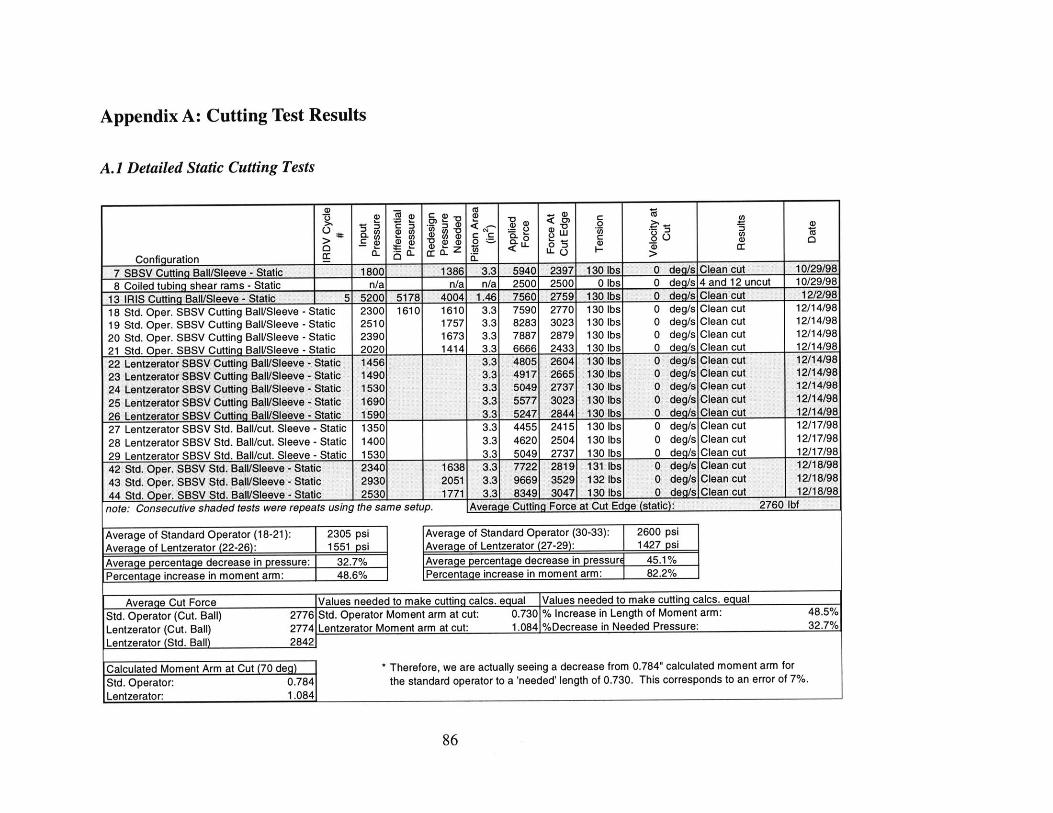
Appendix A: Cutting Test Results

A.1 Detailed Static Cutting Tests

U) = UU a)W

2l U- 0 a)75c1z <

Configuration C [ 0.7 SBSV Cutting Ball/Sleeve - Static 1800 1386 3.3 5940 2397 130 lbs 0 deq/s Clean cut 10/29/988 Coiled tubing shear rams - Static n/a n/a n/a 2500 2500 0 lbs 0 deg/s 4 and 12 uncut 10/29/98

13 IRIS Cutting Ball/Sleeve - Static 5 5200 5178 4004 1.46 7560 2759 130 lbs 0 deq/s Clean cut 12/2/98

18 Std. Oper. SBSV Cutting Ball/Sleeve - Static 2300 1610 1610 3.3 7590 2770 130 lbs 0 deg/s Clean cut 12/14/98

19 Std. Oper. SBSV Cutting Ball/Sleeve - Static 2510 1757 3.3 8283 3023 130 lbs 0 deg/s Clean cut 12/14/98



22 Lentzerator SBSV Cutting BalVSleeve - Static 1456 3.3 4805 2604 130 lbs 0 deg/s Clean cut 12/14/98

23 Lentzerator SBSV Cutting Ball/Sleeve - Static 1490 3.3 4917 2665 130 lbs 0 deg/s Clean cut 12/14/98




27 Lentzerator SBSV Std. Ball/cut. Sleeve - Static 1350 3.3 4455 2415 130 lbs 0 deg/s Clean cut 12/17/98

28 Lentzerator SBSV Std. Ball/cut. Sleeve - Static 1400 3.3 4620 2504 130 lbs 0 deg/s Clean cut 12/17/98

29 Lentzerator SBSV Std. Ball/cut. Sleeve - Static 1530 3.3 5049 2737 130 lbs 0 deq/s Clean cut 12/17/98

42 Std. Oper. SBSV Std. Ball/Sleeve - Static 2340 1638 3.3 7722 2819 131 lbs 0 deg/s Clean cut 12/18/98

43 Std. Oper. SBSV Std. Ball/Sleeve -Static 2930 2051 3.3 9669 3529 132 lbs 0 deg/s Clean cut 12/18/9844 Std. Oper. SBSV Std. Ball/Sleeve - Static 2530 1771 3.3 8349 3047 130 lbs 0 deo/s Clean cut 12/18/98

note: Consecutive shaded tests were repeats using the same setup. Average Cutting Force at Cut Edge (static): 2760 lbf

Average of Standard Operator (18-21): 2305 psi Average of Standard Operator (30-33): 2600 psi

Average of Lentzerator (22-26): 1551 psi Average of Lentzerator (27-29): 1427 psi

Average percentage decrease in pressure: 32.7% Average percentage decrease in pressure 45.1%

Percentage increase in moment arm: 48.6% Percentage increase in moment arm: 82.2%

Average Cut Force Values needed to make cuttinq calcs. equal Values needed to make cuttinq calcs. equal

Std. Operator (Cut. Ball) 2776 Std. Operator Moment arm at cut: 0.730 % Increase in Length of Moment arm: 48.5%

Lentzerator (Cut. Ball) 2774 Lentzerator Moment arm at cut: 1.084 %Decrease in Needed Pressure: 32.7%

Lentzerator (Std. Ball) 2842

Calculated Moment Arm at Cut (70 de) * Therefore, we are actually seeing a decrease from 0.784" calculated moment arm for

Std. Operator: 0.784 the standard operator to a 'needed' length of 0.730. This corresponds to an error of 7%.Lentzerator: 1 .084

86

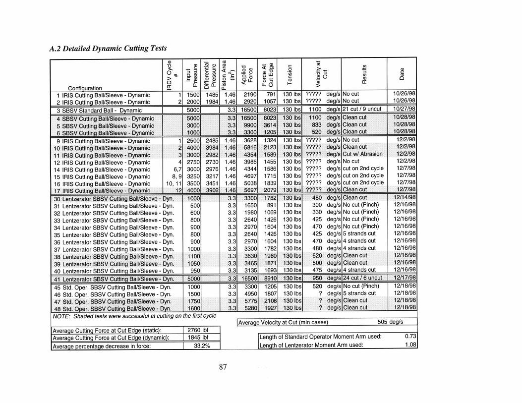
A.2 Detailed Dynamic Cutting Tests

U 3 4-U) a)U 0CJ ) LUU) U)0 U C,,U)

> .C .a) a)) a) 0- U).C

40 O.Cj L- <~ ~ 0 W a) aCc CL U)U a- -D M LL

Configuration C I I

1 IRIS Cutting Ball/Sleeve - Dynamic 1 1500 1485 1.46 2190 791 130 lbs ????? deg/s No cut 10/26/982 IRIS Cutting Ball/Sleeve - Dynamic 2 2000 1984 1.46 2920 1057 130 lbs ????? deg/s No cut 10/26/98

3 SBSV Standard Ball - Dynamic 50001 13.3 1165001 6023 130 lbs 1100 deq/s 21 cut /9 uncut 10/27/98

4 SBSV Cutting Ball/Sleeve - Dynamic 5000 3.3 16500 6023 130 lbs 1100 deg/s Clean cut 10/28/985 SBSV Cutting Ball/Sleeve - Dynamic 3000 3.3 99001 3614 130 lbs 833 deg/s Clean cut 10/28/986 SBSV Cutting Ball/Sleeve - Dynamic 1000 3.3 3300 1205 130 lbs 520 deq/s Clean cut 10/28/98

9 IRIS Cutting Ball/Sleeve - Dynamic 1 2500 2485 1.46 3628 1324 130 lbs ????? deg/s No cut 12/2/9810 IRIS Cutting Ball/Sleeve - Dynamic 2 4000 3984 1.46 5816 2123 130 lbs ????? deg/s Clean cut 12/2/9811 IRIS Cutting Ball/Sleeve - Dynamic 3 3000 2982 1.46 4354 1589 130 lbs ????? deg/s Cut w/ Abrasion 12/2/9812 IRIS Cutting Ball/Sleeve - Dynamic 4 2750 2730 1.46 3986 1455 130 lbs ????? deg/s No cut 12/2/9814 IRIS Cutting Ball/Sleeve - Dynamic 6,7 3000 2976 1.46 4344 1586 130 lbs ????? deg/s cut on 2nd cycle 12/7/9815 IRIS Cutting Ball/Sleeve - Dynamic 8,9 3250 3217 1.46 4697 1715 130 lbs ????? deg/s cut on 2nd cycle 12/7/9816 IRIS Cutting Ball/Sleeve - Dynamic 10, 11 3500 3451 1.46 5038 1839 130 lbs ????? deg/s cut on 2nd cycle 12/7/9817 IRIS Cutting Ball/Sleeve - Dynamic 12 4000 3902 1.46 5697 2079 130 lbs ????? deg/s Clean cut 12/7/98

30 Lentzerator SBSV Cutting Ball/Sleeve - byn. 1000 3.3 3300 1782 130 lbs 480 deg/s Clean cut 12/14/9831 Lentzerator SBSV Cutting Ball/Sleeve - Dyn. 500 3.3 1650 891 130 lbs 300 deg/s No cut (Pinch) 12/16/9832 Lentzerator SBSV Cutting Ball/Sleeve - Dyn. 600 3.3 1980 1069 130 lbs 330 deg/s No cut (Pinch) 12/16/9833 Lentzerator SBSV Cutting Ball/Sleeve - Dyn. 800 3.3 2640 1426 130 lbs 425 deg/s No cut (Pinch) 12/16/9834 Lentzerator SBSV Cutting Ball/Sleeve - Dyn. 900 3.3 2970 1604 130 lbs 470 deg/s No cut (Pinch) 12/16/9835 Lentzerator SBSV Cutting Ball/Sleeve - Dyn. 800 3.3 2640 1426 130 lbs 425 deg/s 5 strands cut 12/16/9836 Lentzerator SBSV Cutting Ball/Sleeve - Dyn. 900 3.3 2970 1604 130 lbs 470 deg/s 4 strands cut 12/16/9837 Lentzerator SBSV Cutting Ball/Sleeve - Dyn. 1000 3.3 3300 1782 130 lbs 480 deg/s 4 strands cut 12/16/9838 Lentzerator SBSV Cutting Ball/Sleeve - Dyn. 1100 3.3 3630 1960 130 lbs 520 deg/s Clean cut 12/16/9839 Lentzerator SBSV Cutting Ball/Sleeve - Dyn. 1050 3.3 3465 1871 130 lbs 500 deg/s Clean cut 12/16/9840 Lentzerator SBSV Cutting Ball/Sleeve - Dyn. 950 3.3 3135 1693 130 lbs 475 deq/s 4 strands cut 12/16/98

41 Lentzerator SBSV Cutting BaL/Sleeve - Dyn. 50001 3.3 165001 89101 130 lbs 950 deg/s 24 cut / 6 uncut 12/17/98

45 Std. Oper. SBSV Cutting Ball/Sleeve - Dyn. 1000 3.3 3300 1205 130 lbs 520 deg/s No cut (Pinch) 12/18/9846 Std. Oper. SBSV Cutting Ball/Sleeve - Dyn. 1500 3.3 4950 1807 130 lbs ? deg/s 5 strands cut 12/18/9847 Std. Oper. SBSV Cutting Ball/Sleeve - Dyn. 150 3.3 457 1808 130 lbs ? deg/s Clean cut 12/18/9847 Std. Oper. SBSV Cutting Ball/Sleeve - Dyn. 1750 3.3 5275 2108 130 lbs ? deg/s Clean cut 12/18/9848 Std. Oper. SBSV Cutting Ball/Sleeve - Dyn. 1600 __ 3.3 52801 1927 130 lbs ?7e/ la cut 12/18/98NOTE: Shaded tests were successful at cutting on the first cycle

I Average Velocity at Cut (min cases) 505 deg/s

Average Cutting Force at Cut Edge (static): 2760 lbfAverage Cutting Force at Cut Edge (dynamic): 1845 lbf Length of Standard Operator Moment Arm used: 0.73

Average percentage decrease in force: 33.2% I Length of Lentzerator Moment Arm used: 1.08

87

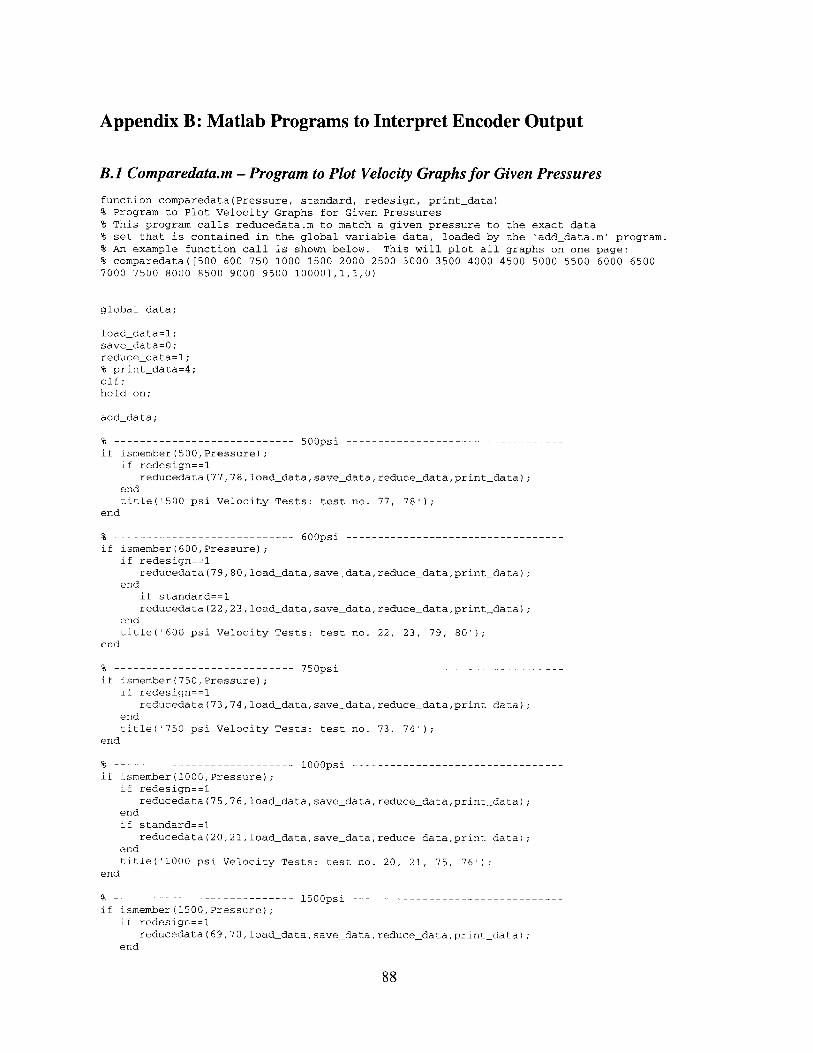
Appendix B: Matlab Programs to Interpret Encoder Output

B.1 Comparedata.m - Program to Plot Velocity Graphs for Given Pressures

function comparedata(Pressure, standard, redesign, print-data)% Program to Plot Velocity Graphs for Given Pressures% This program calls reducedata.m to match a given pressure to the exact data% set that is contained in the global variable data, loaded by the 'adddata.m' program.% An example function call is shown below. This will plot all graphs on one page:% comparedata([500 600 750 1000 1500 2000 2500 3000 3500 4000 4500 5000 5500 6000 65007000 7500 8000 8500 9000 9500 100001,1,1,0)

global data;

load-data=1;save-data=0;reduce data=l;% print-data=4;clf;hold on;

adddata;

% ---------------------------- 500psi ----------------------------------if ismember(500,Pressure);

if redesign==1reducedata(77,78,load data,savedata,reducedata,print-data);

endtitle('500 psi Velocity Tests: test no. 77, 78');

end


if redesign==lreducedata(79,80,load data,savedata,reduce_data,print-data);

endif standard==1reducedata(22,23,loaddatasave_datareduce_data,print-data);

endtitle('600 psi Velocity Tests: test no. 22, 23, 79, 80');

end

% ---------------- 7S0psi-----------------------------------if ismember(750,Pressure);

if redesign==1reducedata(73,74,load data,savedata,reduce_data,print data);

endtitle('750 psi Velocity Tests: test no. 73, 74');

end

% -------- ---------------- 1000psi ---------------------------------if ismember(1000,Pressure);

if redesign==1reducedata(75,76,load data,savedata,reduce_data,print-data);

endif standard==1

reducedata(20,21,load data,save-data,reducedata,print-data);endtitle('1000 psi Velocity Tests: test no. 20, 21, 75, 76');

end

% ---------------------------- 1500psi -------------------- -----if ismember(1500,Pressure);

if redesign==lreducedata(69,70,load data,save data,reducedata,print data);

end

88

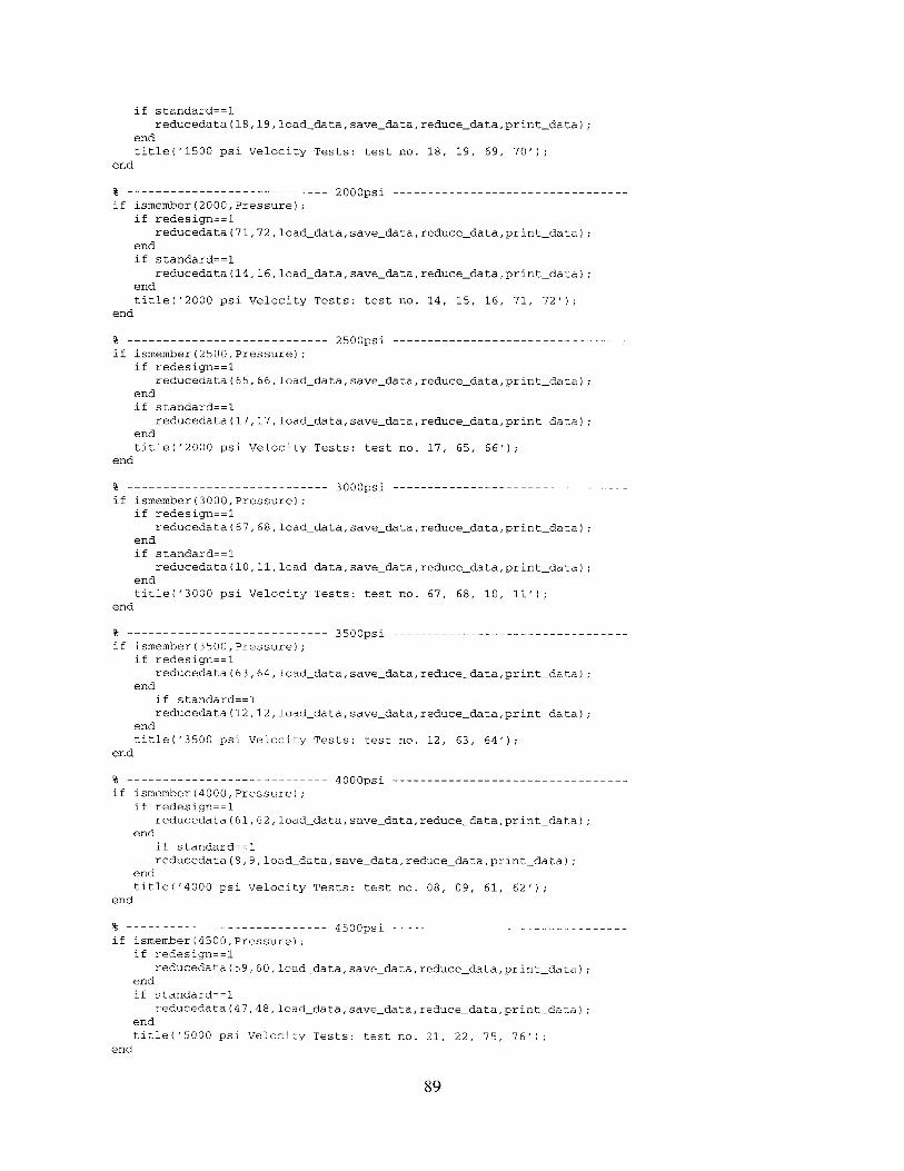
if standard==1reducedata(18,19,load data,savedata,reduce_data,printdata);


end



endif standard==1

reducedata(14,16,load data,savedata,reducedata,print-data);endtitle('2000 psi Velocity Tests: test no. 14, 15, 16, 71, 72');

end


if redesign==1reducedata(65,66,load data,save-data,reduce_data,printdata);

endif standard==1

reducedata(17,17,load-data,savedata,reduce-data,printdata);endtitle('2000 psi Velocity Tests: test no. 17, 65, 66');

end


if redesign==lreducedata(67,68,load-data,savedata,reduce_data,print-data);

endif standard==1

reducedata(10,11,loaddata,savedata,reduce_data,print-data);endtitle('3000 psi Velocity Tests: test no. 67, 68, 10, 11');

end



endif standard==1reducedata (12, 12, load data, savedata,reduce_data,print data);

endtitle('3500 psi Velocity Tests: test no. 12, 63, 64');

end

% --------------------------- 4000psi ---------------------------------if ismember(4000,Pressure);


endif standard==1reducedata(8,9,load data,savedata,reducedata,print data);


end

% ---------------------------- 4500psi ---------------------------------if ismember(4500,Pressure);


endif standard==l

reducedata(47,48,loaddata,savedata,reducedata,print-data);endtitle('5000 psi Velocity Tests: test no. 21, 22, 75, 76');

end

89



endif standard==1reducedata(49,50,load data,savedata,reduce-data,printdata);


end



endif standard==1reducedata(45,46,load data,savedata,reduce_data,print-data);


end

% ---------------------------- 6000psi --------------------------if ismember(6000,Pressure);

if redesign==1reducedata(97,98,load data,save_data,reducedata,print-data);

endif standard==lreducedata(43,44,load data,savedata,reducedata,print-data);


end





end




endtitle('7000 psi Velocity Tests: test no. 24, 25, 26, 93, 94');

end


if redesign==lreducedata(91,92,load data,savedata,reduce_data,printdata);


end

title('7500 psi Velocity Tests: test no. 38, 39, 91, 92');end

% ---------------------------- 8000psi ------------ - ----- - ----if ismember(8000,Pressure);

if redesign==1reducedata(89,90,load-data,save-data,reduce-data,print data);

90

endif standard==l

reducedata(36,36,load data,save-data,reduce-data,print-data);reducedata(40,40,loaddata,savedata,reduce-data,printdata);


end



endif standard==1reducedata(34,35,load data,savedata,reduce_data,printdata);


end


if redesign==lreducedata(85,86,load data,savedata,reducedata,printdata);

endif standard==lreducedata(32,33,load data,save-data,reduce_data,printdata);


end


if redesign==lreducedata(83,84,load-data,savedata,reduce_data,print-data);

endif standard==1reducedata(30,31,load data,save-data,reduce_data,printdata);


end

% ---------------------------- 10000psi --------------------------- ---if ismember(10000,Pressure);

if redesign==1reducedata(81,82,load data,save-data,reduce_data,printdata);


endtitle('10000 psi Velocity Tests: test no. 27, 28, 29, 81, 82');

end

% ---------------------------- 5001 psi Reference ----------------------if ismember(5001,Pressure);

if redesign==lreducedata(121,122,load data,savedata,reducedata,print-data);

endif standard==1reducedata(49,50,load data,savedata,reduce_data,printdata);


end

% ---------------------------- 5002 psi Cut ------------------------- -if ismember(5002,Pressure);

if redesign==lreducedata(123, 123,loaddata,savedata,reducedata,printdata);

endif standard==1reducedata(51,51,load-data,savedata,reducedata,print-data);

91

endtitle('5000 psi Cutting Tests: test no. 51. 123');

end

% ---------------------------- 5055 psi Cutting Sleeve -----------------if ismember(5055,Pressure);


endif standard==lreducedata(133,134,load data,savedata,reducedata,print-data);

endtitle('5000 psi Velocity Tests w/ Cutting Sleeve: test no. 124, 125');

end

% ---------------------------- 3033psi Cutting Sleeve ------------------if ismember(3033,Pressure);


endif standard==1

reducedata(135,136,load data,savedata,reducedata,print-data);endtitle('3000 psi Velocity Tests: test no. 67, 68, 10, 11');

end

% ---------------------------- 1011psi Cutting Sleeve ------------------if ismember(1011,Pressure);


endif standard==1

reducedata(137,138,load data,savedata,reducedata,print-data);endtitle('1000 psi Velocity Tests: test no. 20, 21, 75, 76');

end

% display([data]);hold off;plot(data(:,1),data(:,6), 'kx');

92

B.2 Reducedata.m - Program to Match Data Files With Pressures

function reducedata(start file, end-file, load-data, savedata,...reduce-data, plot-data)

global data;

% This program is called by comparedata.m and calls encoder.m% The purpose of this program is to call encoder.m with the correct file names% given an input pressure used in comparedata.m

% clear data;aveover=3;% Travel(j) Avevel(j) Maxvel(j) Timemeas(j) Timecalc(j)% data(j,l) data(j,2) data(j,3) data(j,4) data(j,5)

if startfile<10if endfile<10for j=startfile:endfile

if loaddata==1load (strcat('tekO00', num2str(j), '.dat'))

endif reduce data==1

[data(j,2) data(j,3) data(j,4) data(j,5) data(j,6)]=...encoder(eval(strcat('tekOO00', num2str(j))), aveover,...strcat('Test #', num2str(j), ' - tekO00', num2str(j)),plot data);

endend

elsefor j=startfile:9if loaddata==1

load (strcat('tekO00', num2str(j), '.dat'))end

if reduce data==l[data(j,2) data(j,3) data(j,4) data(j,5) data(j,6)]=...

encoder(eval(strcat('tekOO00', num2str(j))), aveover,...strcat('Test #', num2str(j), ' - tekO00', num2str(j)),plot-data);

endendfor j=10:endfile

if loaddata==1load (strcat('tekOOO', num2str(j), '.dat'))

endif reduce data==l

[data(j,2) data(j,3) data(j,4) data(j,5) data(j,6)]=...encoder(eval(strcat('tekOOO', num2str(j))), ave-over,...strcat('Test #', num2str(j), ' - tekOOO', num2str(j)),plot_data);

endend

endelseif startfile<100

if endfile<100for j=startfile:endfile

if loaddata==1load (strcat('tekOOO', num2str(j), '.dat'))

endif reduce data==1

[data(j,2) data(j,3) data(j,4) data(j,5) data(j,6)1=...encoder(eval(strcat('tekOOO', num2str(j))), aveover,...strcat('Test #', num2str(j), ' - tekOOO', num2str(j)),plot data);

endend

elsefor j=startjfile:99if loaddata==1

load (strcat('tekOOO', num2str(j), '.dat'))end

if reduce-data==l[data(j,2) data(j,3) data(j,4) data(j,5) data(j,6)]=...

93

encoder(eval(strcat('tekOOO', num2str(j))), aveover,...strcat('Test #', num2str(j), ' - tekOOO', num2str(j)),plotdata);

end

endfor j=100:endfile

if loaddata==lload (strcat('tekOO', num2str(j), '.dat'))

endif reducedata==l

[data(j,2) data(j,3) data(j,4) data(j,5) data(j,6)]=...

encoder(eval(strcat('tekOO', num2str(j))), aveover,...strcat('Test #', num2str(j), ' - tekOO', num2str(j)),plot-data);

endend

end

elsefor j=start file:endfileif load-data==1

load (strcat('tekOO', num2str(j), '.dat'))endif reducedata==l

[data(j,2) data(j,3) data(j,4) data(j,5) data(j,6)]=...encoder(eval(strcat('tekOO', num2str(j))), aveover,...strcat('Test #', num2str(j), ' - tekO0', num2str(j)),plotdata);

endend

endend

94

B.3 Encoder.m - Program to Create Velocity Graphs from Data File

%------------------------- Encoder.m -------------------------------------------

%-- Program to convert the output from a normal incremental encoder

%-- from the frequency domain to the linear position domain. The program

%-- takes four inputs from the command line and outputs the results to five%-- variables and one graph.

%------------------------- Function Initialization ------------------------------

function [a,b,c,d,e] =encoder(encod file, ave-over, test-desc, freq-plot)

% Input Variables:% encod file = Name of variable of encoder data file, i.e. TEK00021% aveover = Number of adjacent points to average over, i.e. 2% test-desc = Description of Test to be printed on graph (put text in 'quotes')% freq-plot = Choose number 1,2,3 for output plot: 1 = Freq, Pos, Ang. Vel

% 2 = Pos, Ang. Vel, Lin. Vel% 3 = Ang. Vel only

% Output Variables:% A = Total calculated angular travel% B = Average angular velocity% C = Maximum angular velocity% D = Closing Time Measured% E = Average Linear closing velocity of operator

%------------------------- Initialize Variables --------------------------------

numchanges=O; % Number of rises or falls of the square waveang=O; % Angle of Ball Rotation (0 degrees at PCT open)sprc-ang-vect=0; % Sparce Angle Vector of Ball Anglessprctime vect=0; % Sparce Time Vector Corresponding to Anglespack-ang-vect=O; % Compacted Angle Vector (zero values removed)packtimevect=O; % Compacted Time Vector (times at zero values removed)filledindex=O; % Indices of Non-Zero Values in Sparce Vectortot_temp-ang=O; % Total Temp Angletottemp-time=0; % Total Temp Timeredang-vect=O; % Reduced Angle Vector (after averaging)redtimevect=0; % Reduced Time Vector (after averaging)vel=0; % Velocity (differentiated from angle data)linvel=0; % Linear Velocity of operator (from Angular Velocity)avelin-vel=0; % Average Linear Velocitypack-vel=0; % Packed Velocitystart time=l; % Init Time (time at start)endtime=0; % Ending Time (time at ending)begin-ave=0; % Index to 15 percent done (begining of vel averaging)endave=O; % Index to 85 percent done (ending of vel averaging)

--- Display Progress Meter% ----------------------disp(['.'));

%-------------------------- Filter Noise From File -----------------------------% disp(length(encodfile));for i=4:length(encod file)

if encodfile(i)>7.5encodfile(i)=15.7;

elseencodfile(i)=0;

end

% if ((encod-file(i)<12) & (encod-file(i)>5))% disp('in the middle');% end

end

%-------------------------- Convert Freq to Position ---------------------------

for j=4:(length(encod_file)-1)if abs(encod-file(j+l)-encodfile(j))>10

num changes=num-changes+l;

95

ang=ang+.17578125;sprcangvect(j)=ang;

endif j==length(encod-file)

sprcangvect(j)=ang;end

end

%-------------------------- Compact Time and Angle Vectors ---------------------% Calculate time vectorsprctimevect=encodfile(2).*(1:length(sprc-ang-vect));

% Calculate indices of non-zero entriesfilledindex=find(sprc-ang-vect);

pack timevect=sprc-time-vect(filled-index);

pack ang vect=sprc-ang-vect (f illedjindex);

%-------------------------- Average Adjacent Points - Reduce -- -----------

for k=l:(length(pack-ang-vect)/ave-over)tottempang=O;tot-temp-time=O;for m=O:(ave-over-1)

tot-tempang=pack-ang-vect((k*aveover)-m)+tottempang;endred-ang-vect(k)=(l/ave-over).*tot-temp-ang;for p=O:aveover-1

tot-temp-time=packtimevect((k*ave-over)-p)+tot-temp-time;endred time vect(k)=(1/ave-over).*tot-temp-time;

end

%-------------------------- Differentiate Angular Position ---------------------

for j=1:(length(redangvect)-2)vel(j)=.5*(abs(redangvect(j+1) -redangvect(j) ) /abs(red-time-vect(j+1)-...

redtime-vect(j)))+.5*(abs(red ang-vect(j+2)-red ang vect(j+l))/ ...abs(red-time-vect(j+2)-redtime-vect(j+l)));

end

for m=l:(length(pack-ang-vect)-2)pack-vel(m)=.5*(abs(pack-ang vect(m+l)-pack-angvect(m))/ ...

abs(packtimevect(m+1)-packtimevect(m)))+.5*(abs(pack-ang-vect(m+2)-...pack-ang-vect(m+l))/abs(pack-timevect(m+2)-pack-time-vect(m+l)));

end

for n=1:length(vel)lin-vel(n)= vel(n)./(-0.0135.*red-ang-vect(n).*red-ang-vect(n)+1.244.*...

red-ang-vect(n)+31);end

%-------------------------- Calculate Vel. and Time ----------------------------begin ave=round(length(red-ang-vect)*.15);endave=round(length(red-ang-vect)*.85);ave linvel=mean(linvel(begin-ave:endave));

for n=4:(length(pack-vel)-l)

if pack vel(n)-pack vel(n-3)>0.15*max(vel)if pack timevect(n)<start time

start-time=packtimevect(n);% disp(['Init Time: num2str(start-time)));

endend

if pack vel(n-2)-pack-vel(n+)>0.15*max(vel)if pack-time-vect(n)>end time

endtime=pack time vect(n);end

end

end

96

%-------------------------- Plot Results ---------------------------------------

%--l--Plot results with Frequency graph, Position Graph and Velocity Graph -----

if freq-plot==lsubplot(3,1,1);plot(sprc-time-vect(4:length(sprctimevect)),...

encodfile(4:length(sprc time vect)));

axis([0, max(sprc-time vect), -1, (max(encod-file(4:length(encodjfile)))+1)]);

ylabel('Output Voltage (V)', 'Fontsize', 10);

if -isempty(test-desc)title([num2str(test-desc),' - (Average over=', num2str(ave-over), ')']);

endxlabel('Time (s)')

subplot(3,1,2);plot(red-time-vect,red-ang-vect);axis([0, max(sprc-time-vect), 0, (max(red-ang vect)+5)]);

ylabel('Angular Position (deg)', 'Fontsize', 10);

xlabel('Time (s)')

subplot(3,1,3)plot(red-angvect(l:length(vel)),vel)axis([0, max(red-angvect), 0, (max(vel)+100)]);

xlabel('Angular Position (deg)')

ylabel('Angular velocity (deg/s)')

end

%--2--Plot results with Position, Ang. Velocity, and Lin. Velocity Graphs ------if freqplot==2

subplot (3, 1, 1)plot(red time vect,red-ang-vect);

axis([0, max(sprc-time-vect), 0, (max(red-ang-vect)+5)]);ylabel('Angular Position (deg)', 'Fontsize', 10);

if -isempty(test-desc)title([num2str(test-desc),' - (Average over=', num2str(ave-over), ')']);

endxlabel('Time (s)');

subplot(3,1,2)plot(red-ang vect(l:length(vel)),vel)axis([0, max(red-angvect), 0, (max(vel)+100)]);

ylabel('Angular velocity (deg/s)')xlabel('Angular Position (deg)')

subplot(3,1,3);plot(red-angvect(:length(vel)),lin-vel);ylabel('Velocity of Operator (in/s)', 'Fontsize', 10);xlabel('Angular Position (deg)')

end

%--3--Plot results with Angular Velocity Graph Only --- -------------------if freqplot==3

subplot(1,1,1)plot(red ang-vect(l:length(vel)),vel, '-k')

axis([0, max(red-angvect), 0, (max(vel)+100)]);xlabel('Angular Position (deg)')

ylabel('Angular velocity (deg/s)')if -isempty(testdesc)

title([num2str(test-desc),' - (Average over=', num2str(ave-over), ')']);end

end

%--4--Plot results with Linear Velocity Graph Only -------- -----------if freqplot==4

subplot(1,1,1)plot(red ang-vect(l:length(vel)),linvel);xlabel('Angular Position (deg)')

ylabel('Velocity of Operator (in/s)', 'Fontsize', 10);

if -isempty(test-desc)

97

title([num2str(test-desc),' - (Average over=', num2str(aveover), ')']);end

end

%--5--Output results to file for graphing in Excel -----------------------------

if freq-plot==5outl=redangvect;out2=vel;out3=linvel;save velcocity-profile2000std.dat outl out2 out3 -ascii -tabs

end

%-------------------------- Output Variables -----------------------------------

a=numchanges/2*360/1024;b=mean(vel);c=max(vel);d=endtime-start-time;e=ave-lin-vel;

98

B.4 AddData.m - Data Set that Matches Data Sets to Pressures

function add-data()

% This function creates a vector called 'data' that is used as a database% for reducedata.m. The numbers on the right of the equation are the input pressures% and the index of the vector is the sequential test that was performed.

global data;

data(1,1)=3015;data(2,1)=1000;data(3,1)=3085;data(4,1)=3071;data(5,1)=4018;data(6,1)=5035;data(7,1)=5035;data(8,1)=4035;data(9,1)=3995;data(10,1)=3005;data(11,1)=3035;data(12,1)=3500;data(13,1)=3500;data(14,1)=2000;data(15,1)=2000;data(16,1)=2000;data(17,1)=2500;data(18,1)=1500;data(19,1)=1500;data(20, 1) =1000;data(21,1)=1000;data(22,1)=600;data(23,1)=600;data(24,1)=7000;data(25,1)=7000;data(26,1)=7000;data(27,1)=10000;data(28,1)=10000;data(29,1)=10000;data(30,1)=9500;data(31, 1)=9500;data(32,1)=9000;data(33,1)=9000;data(34,1)=8500;data(35,1)=8500data(36,1)=8000;data (37,1) =8000;data (38,1) =7500;data(39,1)=7500;data(40,1)=8000;data(41,1)=6500;data(42,1)=6500;data(43,1)=6000;data(44,1)=6000;data(45,1)=5500;data(46, 1)=5500;data(47,1)=4500;data(48, 1)=4500;data(49,1)=5000;data(50,1)=5000;data(51,1)=5000;data(52,1)=5000;data(53,1)=3000;data(54,1)=1000;data(55,1)=1800;data(56,1)=3000;data(57,1)=5000;data(58,1)=5000;data(59, 1) =4500;

99

data(60,1)=4500;data(61,1)=4000;data(62,1)=4000;data(63,1)=3500;data(64,1)=3500;data(65,1)=2500;data(66,1)=2500;data(67,1)=3000;data(68,1)=3000;data(69,1)=1500;data(70,1)=1500;data(71,1)=2000;data(72,1)=2000;data(73,1)=750;data(74,1)=750;data(75,1)=1000;data(76,1)=1000;data(77,1)=500;data(78,1)=500;data(79, 1) =600;data(80,1)=600;data(81,1)=10000;data(82,1)=10000;data(83,1)=9500;data(84,1)=9500;data(85,1)=9000;data (86,1) =9000;data(87,1)=8500;data(88,1)=8500;data(89,1)=8000;data(90,1)=8000;data (91,1) =7500;data(92,1)=7500;data(93,1)=7000;data(94, 1)=7000;data(95,1)=6500;data(96,1)=6500;data(97,1)=6000;data(98,1)=6000;data (99,1) =5500;data(100,1)=5500;data(101,1)=500;data(102,1)=500;data(103,1)=500;data(104,1)=500;data(105,1)=500;data(106,1)=500;data(107,1)=500;data (108,1) =500;data(109,1)=500;

100

Optimization of a Pin-and-Slot Ball Valve Linkage - DSpace ...

Documents

Transcript of Optimization of a Pin-and-Slot Ball Valve Linkage - DSpace ...