Optimalizace vybrané části posilovače řazení vozů TATRA pro ...

VŠB – Technical University of Ostrava

Faculty of Mechanical Engineering

Department of Applied Mechanics

Optimalizace vybrané části posilovače

řazení vozů TATRA pro 3D tisk

Optimization of Selected Gearshift Booster

Part of TATRA Vehicles for 3D Printing

Student: Aldabash Tariq

Diploma thesis supervisor: prof. Ing. Radim Halama, Ph.D.

Ostrava 2019/2020

ANNOTATION OF DIPLOMA THESIS

ALDABASH TARIQ. Optimization of Selected Gearshift Booster Part of TATRA

Vehicles for 3D Printing. Ostrava: VŠB – Technical University of Ostrava, Faculty of

Mechanical Engineering, Department of Applied Mechanics, 2020, 72 p. Thesis head: prof.

Ing. Radim Halama, Ph.D.

This thesis describes the design procedure of a main shifting thumb in a gearshift booster

using several topology optimization methods and software which has been created to support

additive manufacturing. The thesis is divided into three main parts. The first part is a

familiarization with the different types of systems that are used by TATRA trucks. The

following section deals with topology optimization methods and the application of topology

optimization using ANSYS software. The final part deals with additive manufacturing

preparation, process and experimental validation.

Keywords: TATRA, Shift booster, topology optimization, additive manufacturing, SLM,

FEM

ANOTACE DIPLOMOVÉ PRÁCE

ALDABASH TARIQ. Optimalizace vybrané části posilovače řazení vozů TATRA pro 3D

tisk. VŠB-TU Ostrava, Fakulta strojní, Katedra aplikované mechaniky, 2020, 72 s. Vedoucí

diplomové práce: prof. Ing. Radim Halama, Ph.D.

Tato práce popisuje postup návrhu hlavního řadícího palce v posilovači řazení pomocí

několika optimalizačních metod topologie a softwaru, který byl vytvořen pro podporu aditivní

výroby. Práce je rozdělena do tří hlavních částí. V první části je seznámení s různými typy

systémů, které jsou používány nákladními vozidly TATRA. Následující část se zabývá

metodami topologické optimalizace a aplikací topologické optimalizace pomocí software

ANSYS. Závěrečná část se zabývá přípravou aditivní výroby, vlastním zpracováním a

experimentální validací.

Klíčová slova: TATRA, posilovač řazení, topologická optimalizace, additivní výroba, SLM,

MKP

Table of Contents

1 Introduction ............................................................................................................. 13

2 Related Technical Details of TATRA Trucks ....................................................... 16

2.1 Study Related TATRA trucks ............................................................................ 16

2.1.1 TATRA FORCE ......................................................................................... 16

2.1.2 TATRA TERRA ......................................................................................... 17

2.2 Used Transmissions for TATRA Trucks ........................................................... 18

2.2.1 TATRA 10TS/14TS ................................................................................... 18

2.2.2 TATRA-NORGREN .................................................................................. 19

2.2.3 Transfer case of TATRA ............................................................................ 20

2.3 Used shift boosters for TATRA trucks .............................................................. 21

2.3.1 Pneumatic shift boosters ............................................................................. 22

2.3.2 Hydraulic shift boosters .............................................................................. 22

2.3.3 Electro-mechanical shift boosters ............................................................... 23

2.4 TATRA 14TS210 gearbox boosters .................................................................. 23

2.4.1 TATRA mechanical-pneumatic booster ..................................................... 23

2.4.2 Pneumatic booster TATRA-NORGREN.................................................... 25

3 Topology Optimization ........................................................................................... 27

3.1 Geometry of Model ............................................................................................ 28

3.2 Material of Model .............................................................................................. 29

3.3 Mesh of Model ................................................................................................... 30

3.4 Static Structural Analysis System Setup and Solution ...................................... 31

3.5 The SIMP Method on ANSYS Workbench ....................................................... 34

3.5.1 Advantages and Disadvantages of SIMP Method ...................................... 34

3.5.2 Mathematical model ................................................................................... 35

3.5.3 ANSYS setup and results ........................................................................... 36

3.5.3.1 Setup Overview ....................................................................................... 36

3.5.3.2 Topology Optimization Setup and Results ............................................. 38

3.5.3.3 Smoothing and Validation of the Results ............................................... 42

3.6 The Level-Set Method on ANSYS Workbench ................................................. 43

3.6.1 Advantages and Disadvantages of Level Set Method ................................ 44

3.6.2 Mathematical model ................................................................................... 44

3.6.3 ANSYS setup and results ........................................................................... 46

3.6.3.1 Setup Overview ....................................................................................... 46

3.6.3.2 Topology Optimization Setup and Results ............................................. 47

3.6.3.3 Smoothing and Validation of the Results ............................................... 51

3.7 Other Approaches .............................................................................................. 52

3.8 Selection of Printed Part .................................................................................... 56

4 Additive Manufacturing ......................................................................................... 57

4.1 Types of Additive Manufacturing Technologies ............................................... 57

4.2 Selective Laser Melting (SLM) ......................................................................... 57

4.3 Renishaw AM 400 Additive Manufacturing System ......................................... 58

4.4 Materials Used for 3D Printing .......................................................................... 59

4.5 ANSYS Printing Setup and Thermal Analysis .................................................. 60

4.6 Printing Results .................................................................................................. 64

4.7 Testing................................................................................................................ 65

4.7.1 Setup ........................................................................................................... 65

4.7.2 Results ........................................................................................................ 66

5 Conclusion ................................................................................................................ 67

6 Bibliography ............................................................................................................ 70

List of Figures

Figure 1 Gear Shift - TATRA FORCE [1] ....................................................................... 14

Figure 2 Gear Shift Detail - TATRA FORCE [1] ............................................................ 14

Figure 3 Shifter mechanism - TATRA TERRA [1] ......................................................... 15

Figure 4 TATRA FORCE – Recovery [2] ........................................................................ 17

Figure 5 TATRA TERRA 8x8 [2] ................................................................................... 18

Figure 6 14TS210L gearbox fitted with TATRA mechanical-pneumatic booster [1] ..... 19

Figure 7 TATRA 14TS210T-N gearbox fitted with TATRA-NORGREN [2] ................ 20

Figure 8 Shift selector for TATRA-NORGREN [7] ........................................................ 20

Figure 9 Gear shift fork 14TS210 including original thumb [4] ...................................... 21

Figure 10 Original mechanical-pneumatic booster TATRA [1] ....................................... 24

Figure 11 TATRA pneumatic booster section [6] ............................................................ 24

Figure 12 Power steering TATRA-NORGREN [7] ......................................................... 25

Figure 13 TATRA-NORGREN in neutral position [4] .................................................... 26

Figure 14 TATRA-NORGREN in second gear [4] .......................................................... 26

Figure 15 Topology optimization cycle [5] ...................................................................... 27

Figure 16 Original geometry of main shifting thumb [Author] ........................................ 28

Figure 17 Modified geometry of main shifting thumb [Author] ...................................... 28

Figure 18 Experimental stress-strain curve of 316 stainless steel [Author] ..................... 29

Figure 19 Modulus of elasticity graph [Author] ............................................................... 29

Figure 20 Implemented material data into ANSYS [Author] ........................................... 30

Figure 21 Mesh of the main shifting thumb [Author] ...................................................... 30

Figure 22 General overview of applied constraints [Author] ........................................... 31

Figure 23 Applied force location [Author] ....................................................................... 31

Figure 24 Applied force values [Author] .......................................................................... 31

Figure 25 Fixed support location [Author] ....................................................................... 32

Figure 26 Cylindrical support location [Author] .............................................................. 32

Figure 27 Displacement location [Author] ....................................................................... 32

Figure 28 Static structural analysis setting [Author] ........................................................ 33

Figure 29 Equivalent (Von-Mises) stress [Author] .......................................................... 33

Figure 30 Total deformation [Author] .............................................................................. 33

Figure 31 SIMP method constraints [Author] .................................................................. 37

Figure 32 Calculation layout [Author] ............................................................................. 37


Figure 34 Topology optimization analysis settings SIMP method [Author] .................... 38

Figure 35 Optimization region settings and method selection [Author] .......................... 39

Figure 36 Objective settings [Author] .............................................................................. 39

Figure 37 Mass constraint [Author] .................................................................................. 39

Figure 38 Mass constraint setup [Author] ........................................................................ 39

Figure 39 Symmetry constraint Y-axis [Author] .............................................................. 40

Figure 40 Symmetry constraint Y-axis setup [Author] .................................................... 40

Figure 41 Symmetry constraint X-axis [Author] .............................................................. 40

Figure 42 Symmetry constraint X-axis setup [Author] .................................................... 41

Figure 43 Solution information [Author] ......................................................................... 41

Figure 44 Convergence graph [Author] ............................................................................ 41

Figure 45 Final iteration 12 of solution [Author] ............................................................. 42

Figure 46 Smoothing in Mechanical ANSYS [Author] ................................................... 42

Figure 47 Smoothing in SpaceClaim [Author] ................................................................. 42

Figure 48 Equivalent Von-Mises stress evaluation [Author] ........................................... 43

Figure 49 Level-Set method constraints [Author] ............................................................ 46

Figure 50 Calculation layout [Author] ............................................................................. 46


Figure 52 Topology optimization analysis settings Level-set method [Author] .............. 47

Figure 53 Optimization region settings and method selection [Author] .......................... 48

Figure 54 Objective settings [Author] .............................................................................. 48

Figure 55 Mass constraint [Author] .................................................................................. 48

Figure 56 Mass constraint setup [Author] ........................................................................ 48

Figure 57 Solution information [Author] ......................................................................... 49

Figure 58 Convergence graph [Author] ............................................................................ 49

Figure 59 Iteration 3 of solution [Author] ........................................................................ 50

Figure 60 Final iteration 22 of solution [Author] ............................................................. 50

Figure 61 Smoothing in Mechanical ANSYS [Author] ................................................... 51

Figure 62 Smoothed geometry in SpaceClaim [Author] .................................................. 51

Figure 63 Equivalent Von-Mises stress evaluation [Author] ........................................... 51

Figure 64 ANSYS Discovery Live structural constraints [Author] .................................. 52

Figure 65 Topology optimization result (volume reduction 60%) [Author] ................... 53

Figure 66 Topology optimization result (volume reduction 65%) [Author] .................... 53



Figure 69 Final geometry (trial 3) [Author] ..................................................................... 54

Figure 70 Symmetry and smoothing modifications [Author] ........................................... 55

Figure 71 Validation of trial 3 with 63% reduction [Author] ........................................... 55

Figure 72 Stainless steel square hollow section (SHS) member built using SLM [15] ... 57

Figure 73 Selective Laser Melting process [21] ............................................................... 58

Figure 74 AM 400 additive manufacturing system [20] .................................................. 58

Figure 76 Orientation map [Author] ................................................................................. 60

Figure 77 Selected orientation [Author] ........................................................................... 60

Figure 78 Chessboard print strategy [26] ......................................................................... 61

Figure 79 Additive Manufacturing thermal analysis setup [Author] ................................ 62

Figure 80 AM thermal analysis mesh [Author] ................................................................ 62

Figure 81 AM thermal analysis [Author] ......................................................................... 62

Figure 82 AM Structural analysis [Author] ...................................................................... 63

Figure 83 Standalone structural analysis [Author] ........................................................... 63

Figure 84 Part printing under process [Author] ................................................................ 64

Figure 85 Residual powder material removal [Author] .................................................... 64

Figure 86 Printed part with supports and base plate [Author] .......................................... 64

Figure 87 Cameras used for testing and setup [Author] ................................................... 65

Figure 88 Setup during cutting process [Author] ............................................................. 65

Figure 89 Top and bottom sides after cutting [Author] .................................................... 66

Figure 90 Maximum displacement – left and right cameras [Author] ............................. 66

List of Tables

Table 1 Engines and gearboxes used in the FORCE model [3] ...................................... 16

Table 2 Engines and gearboxes used in the TERRA model [8] ...................................... 17

Table 3 Advantages and disadvantages of pneumatic booster [1] .................................... 22

Table 4 Advantages and disadvantages of hydraulic booster [1] .................................... 22

Table 5 Advantages and disadvantages of electromechanical boosters [1] ...................... 23

Table 6 Topology optimization analysis settings [Author]. ............................................. 52

Table 7 Table of trials [Author] ........................................................................................ 54

Table 8 Mechanical properties of SS 316L-040 [22] ....................................................... 59

Table 9 3D Printing parameters [25] ................................................................................ 61

List of abbreviations and symbols used

𝑥𝑖 – Element density

𝐸𝑖 – Elastic modulus of an element (Young’s modulus)

𝐸0 – Elastic modulus of the solid material

𝐸𝑚𝑖𝑛 – Elastic modulus of the void material

𝑝 – Penalization power (𝑝 > 1)

𝑁𝑖 – Neighbourhood of an element

𝑣 – Volume of an element

𝐻𝑖𝑗 – Weight factor

𝑅 – Size of neighbourhood of filter size

�̃� – Filtered density

𝑒(𝑢) – Total strain vector

𝑒𝑡ℎ – Thermal strain vector

𝜎(𝑢) – Stress vector

(𝑓, 𝑔) – External loads

𝜆𝑢 – Reaction forces

𝑢0 – Prescribed displacement

𝐽(Ω) – Compliance function

1 Introduction

The transmission is one of the key parts of the vehicle drivetrain, which ensures the

transmission of torque further to the wheels. Gear ratios of individual gears significantly affect

the driving characteristics of the vehicle and fuel consumption. For the comfort of driving and

easier operation of the vehicle, especially in difficult terrain, the way of shifting gears is

important. It can be manual, automatic or semi-automatic. TATRA first used manual

transmissions of its own design in its vehicles with parameters optimized for both off-road and

road driving. Later, according to customer requirements, the Twin Disc and Allison automatic

transmissions were built into their vehicles. Using its own mechanical gearboxes and in

cooperation with NORGREN, it has developed semi-automatic transmissions.

The thesis is focused on design of a shifting thumb of a mechanical-pneumatic power

steering, which will be used on manual transmissions TATRA 14TS210L, by utilizing topology

optimization methods to achieve optimum shape. Afterward, manufacturing the part using the

technology of Selective Laser Melting (SLM) to 3D print the desired part in stainless-steel

material then evaluate the structural rigidity of the part and the manufacturability as a 3D

printed part.

The gear shifter booster has high demands on functionality and reliability, as it is one of

the important elements of the powertrain. Failure of such a system can endanger the lives not

only of the vehicle operator but also the surrounding lives nearby the vehicle. Of course,

manufacturing intensity must be taken into consideration, which goes hand in hand with the

overall price of the booster and this is an important factor for the proposal of such equipment.

The booster is designed by my colleague Ing. Machálek Filip and was only consulted with

the design department of TATRA TRUCKS a.s. [1] with the vision to mount this booster on

TERRA and FORCE models fitted with 14TS210 gearboxes in 2020. However, further more

developmental study was raised by TATRA TRUCKS a.s. in order to implement new

manufacturing capabilities such as additive manufacturing.

The advantage of this new design of thumb shifter is to ensure the part durability whilst

using one of the latest technologies in the market. This will increase the overall reliability and

safety of the vehicle during operation, as it eliminates the possibility of a wrong gear shift.

Topology optimization has a big role in order to find the optimum design of the part. Therefore,

there will be a dedicated section that explain the methods used to find the optimum shape using

ASNSYS Workbench and compare obtained results with other software such as ANSYS

Discovery Live.

Figure 1 Gear Shift - TATRA FORCE[1]

Figures 1-3 show the shift mechanism of the TATRA FORCE. The driver of the vehicle

controls the shift lever (No. 1), which is mounted in the articulated mechanism (No. 2). Control

is done by means of Bowden cables, which are attached to this mechanism. In the case of the

selector movement, i.e. by moving the lever left / right, the force is transmitted through the

articulated mechanism and the selector lever (No. 8), which is attached to the end of the dial

by the ball pin (No. 7). The shifting movement, i.e. the forward / reverse movement of the

lever, is transmitted to the shift Bowden (No. 4) by means of a ball pin (No. 6) located on the

shift lever bar. The gearshift bracket (No. 3) ensures that the Bowden cables and the entire

gearshift system are securely attached to the cab.

Figure 2 Gear Shift Detail - TATRA FORCE[1]

Since 2016, when the mechanism has been upgraded, gearbox shifting is ensured by a

combination of Bowden and fixed linkages, as the shift rod would not be able to perform both

the necessary movements due to the various stops. The choice thus remained controlled by a

Bowden cable attached to the power lever, the shifting itself is controlled by a pull rod.

Figure 3 Shifter mechanism - TATRA TERRA[1]

The Figure 3 shows the shift mechanism of the TATRA TERRA vehicle. The vehicle

driver operates the shift lever (No. 1). If the shift lever is selected, i.e. the left / right movement,

the bar (No. 3) transmits the movement by rotation. In the case of shifting, i.e. a forward /

reverse movement, the movement is transmitted to the sliding movement of the bar. The

mechanism (No. 4) is attached to the console (No. 5) to form a support for this shift system.

This mechanism converts the movements of the bar (No. 3) into similar movements of the bar

(No. 7), i.e. the shifting movement is sliding and selecting rotary except for the opposite

rotation provided by the bar (No. 6). The substantial mechanism (No. 2) allows the cab to be

safely tilted without having to disconnect and then engage the shift linkage system. This

shifting mechanism excels in its built-in dimensions, low production cost and precise control.

The disadvantage is the complex kinematic linkages used on the mechanism.

2 Related Technical Details of TATRA Trucks

2.1 Study Related TATRA trucks

TATRA offers manual, semi-automatic or fully automatic gearboxes, but this work is

mainly focused on the semi-automatic 14TS210 gearbox. This type of transmission is only

available on TERRA and FORCE models.

2.1.1 TATRA FORCE

FORCE trucks (Figure 4) are mainly used for special purposes. The former model name

is 815-7 and this type has been produced since 2008 to this day. Most trucks are used in the

armament industry, fire brigade, or oil industry. The differences in vehicles are not only in the

type of body used, but also in the different number of axles, cab, armour and more see Table

1.

Table 1 Engines and gearboxes used in the FORCE model[3]

Model Motor Transmission

FORCE (T815-7)

TATRA T3-928

TATRA 14TS

- manual, 14 speed

TATRA-NORGREN

- semi-automatic, 14 speed

Allison 4500

- automatic, 6 speed

Cummins ISL/ISM

TATRA 14TS

- manual, 14 speed

TATRA-NORGREN


Allison 4500


Figure 4 TATRA FORCE – Recovery[2]

2.1.2 TATRA TERRA

The truck is produced in many variants. It varies according to the number of axles and

body type. It will be used in many industries, such as agriculture, mining, firefighting, military

and others. TATRA TERRA (Figure 5), originally under the designation T815, is a model

manufactured since 1983. When the owners of the company also changed the factory

designation to TATRA TERRA. It comes in several configurations shown in Table 2.

Table 2 Engines and gearboxes used in the TERRA model [8]

Model Motor Transmission

TERRA (T815-2)

TATRA T3-928

TATRA 14TS

- manual, 14 speed

TATRA-NORGREN


Allison 4500


(Rarely used)

Cummins ISL/ISM

(Rarely used)

TATRA 14TS

- manual, 14 speed

TATRA-NORGREN


Allison 4500


Figure 5 TATRA TERRA 8x8 [2]

2.2 Used Transmissions for TATRA Trucks

2.2.1 TATRA 10TS/14TS

TATRA basic gearbox is a manually operated 10TS170 gearbox, which is mounted

directly on the vehicle's auxiliary transmission housing. This becomes an integrated part of the

chassis. The 10TS and 14TS gearboxes differ in the number of gears (10-speed 10TS and 14-

speed 14TS) in combination with a two-speed or a one-speed auxiliary transmission, and of

course differ in the range and scale of individual gears.

The transmission itself provides only five forward and one reverse gears. Their distribution

is guaranteed by a two-stage reduction, which is shifted using electro-pneumatic switch, which

is located on the shift lever of the driver. With this reduction, the transmission already reaches

10 degrees forward and 2 reverse. The gears are synchronized, but with the exception of reverse

and special slow travel marked as C (Crawler), which is used in situations when the vehicle is

stuck or starting off with a fully loaded vehicle. Fourteen gears are thus achieved by dividing

the two fastest gears (with an input reduction of four), either with the range reduction engaged

in the additional gear for slow driving or when the range reduction is engaged in fast driving.

This will allow us to shift fourteen forward gears and two reverse gears. The advantage of this

gearbox is the maximum transmitted torque, which is 2,100 Nm[1].

Figure 6 14TS210L gearbox fitted with TATRA mechanical-pneumatic booster[1]

The benefit of this design is to reduce specific fuel consumption and increase transport

speed. Fourteen gears allow a wider range of gear and thus allow to optimize engine speed to

the desired vehicle speed by utilizing lower engine speeds with higher torque. A secondary

advantage is to reduce the impact stress of the entire drive tract due to the shifting (Figure 6).

2.2.2 TATRA-NORGREN

TATRA-NORGREN automated gearbox can be used to increase driver comfort and speed

up gear shifting (Figure 7). This system employs an electro-pneumatic power shift, which shifts

individual gears. It is based on TATRA 10TS or 14TS gearbox (Figure 8).

The power steering itself increases the driver's comfort to a certain extent, increases the

safety of operation and reduces the risk of damage in the event of incorrect gear changes. The

transmission has two basic shift modes, i.e. manual and automatic. The automatic mode is

divided into AE, AM, AP, AS and MB modes which discussed further in 2.4.2.

Figure 7 TATRA 14TS210T-N gearbox fitted with TATRA-NORGREN[2]

Figure 8 Shift selector for TATRA-NORGREN[7]

2.2.3 Transfer case of TATRA

TATRA mounts transfer case gearboxes on its vehicles, which are used to transmit torque

from the gearbox to a section of the drive train located in the central support pipe. Transfer

case is produced in two variants namely single-speed and two-speed, allowing better

optimization of engine operating speed not only when driving on paved roads and roads, but

also when moving in difficult terrain. This gearbox can only be shifted at a standstill. The

Transfer case is also combined with the ZF and Allison gearboxes. Depending on the selected

type, the gear ratio changes in the transfer case gearbox.

2.3 Used shift boosters for TATRA trucks

The shift booster is usually fixed to the gearbox. Such a mechanism can be powered by

different systems. Mechanically, pneumatically, hydraulically, with the help of electric motors

or a combination of these systems. However, the power steering is not included in the

transmission.

In a pneumatic or hydraulic system, pistons are hidden inside the booster body (usually

the casting) by means of which the shifting elements can be moved. In an electric motor-driven

servo booster, the shift elements are part of the shaft that exists in the system.

The primary function of the power shift is to increase driver comfort, increase operational

safety, and reduce the likelihood of gearbox misalignment. A typical example is the TATRA

14TS210 gearbox, in which a 4580 N force is required on the gearshift to engage a gear and

410 N to select a thumb movement[1]. In the absence of a booster, it would be a difficult gear

selection or impossible in some conditions.

In older trucks, without this system, it was difficult to classify, as the accumulation of

power was solved by a long gear lever. The moment of levering between the shift lever and the

shift element helped to shift more easily, but the long shift lever required the operator's feel

and experience to precisely position the gear (Figure 9).

The first application of the power-assisted steering of TATRA vehicles appeared on the

T138. The system was electro-pneumatic and was used to boost shifting on the auxiliary

transmission. In the present, TATRA trucks use pneumatic or mechanical-pneumatic shifting

boosters.

Figure 9 Gear shift fork 14TS210 including original thumb[4]

2.3.1 Pneumatic shift boosters

The pneumatic shifter works with compressed air, which generates the required force using

a pneumatic engine. Its advantages and disadvantages are displayed in Table 3.

Table 3 Advantages and disadvantages of pneumatic booster [1]

Advantages Disadvantages

- Easier wiring system - Large piston dimensions

- Environmentally friendly in case of system failure - Compressor medium required

- The medium used is available for free - Lower overall efficiency

- The medium can be used from the central distribution - More expensive operation

- No air return is required

- Fast response to the control signal

- High movement frequencies (high speed of

compressed air flow)

2.3.2 Hydraulic shift boosters

The hydraulic booster works with a pressurized fluid that generates the required power

with the hydro-motor. Its advantages and disadvantages are displayed in Table 4.

Table 4 Advantages and disadvantages of hydraulic booster [1]


- Small dimensions of the piston - More expensive operation

- The medium is incompressible - Lower overall efficiency

- Higher efficiency of the hydro-motor - The need for liquid return

- Faster response - The price of hydraulic oil

- Ecologically harmful in case of leakage

2.3.3 Electro-mechanical shift boosters

The electro-mechanical shifter uses electric energy to move it, which is converted into

mechanical energy by an electric motor. Its advantages and disadvantages are displayed in

Table 5.

Table 5 Advantages and disadvantages of electromechanical boosters [1]


- Simpler design - High price

- Ecologically harmless in case of failure

- Quick response to control signal

- Independence from engine operation

2.4 TATRA 14TS210 gearbox boosters

The gearbox TATRA 14TS210 can be fitted with two types of shifting boosters. The first

one is TATRA-pneumatic booster. The transmission with this shifting booster is called

14TS210L. The second is the electro-pneumatic booster TATRA-NORGREN. In this

configuration, the gear unit is referred to as 14TS210T-N.

2.4.1 TATRA mechanical-pneumatic booster

The mechanical-pneumatic booster TATRA is classified into the category of manual

shifting systems. Gear selection and shifting is classic, just like any passenger car equipped

with a manual transmission. Shifting the gear begins by pressing the clutch pedal, then shifting

the desired gear on the shift lever and then gradually releasing the clutch pedal. The shift lever

therefore performs a total of four movements from the neutral position: right, left, front and

back. This movement is transmitted by means of Bowden or rods to the shift servo in which

the final force is transferred to the gear shifting thumb, the element that controls the forks of

the gearbox. In the original version (Figures 10-11), the rotary motion of the thumb is used to

select the fork and the sliding motion is used to shift the gear itself. The fork selection is thus

performed by sliding the shift lever right / left and shifting the speed by sliding forward /

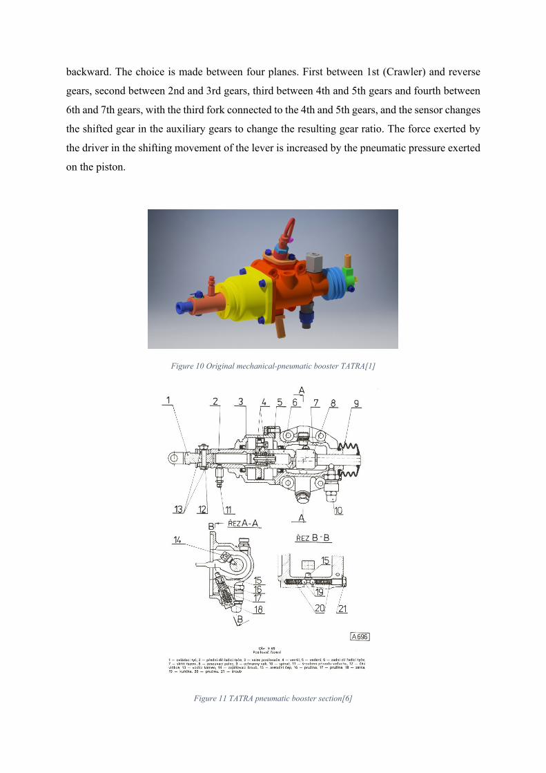
backward. The choice is made between four planes. First between 1st (Crawler) and reverse

gears, second between 2nd and 3rd gears, third between 4th and 5th gears and fourth between

6th and 7th gears, with the third fork connected to the 4th and 5th gears, and the sensor changes

the shifted gear in the auxiliary gears to change the resulting gear ratio. The force exerted by

the driver in the shifting movement of the lever is increased by the pneumatic pressure exerted

on the piston.

Figure 10 Original mechanical-pneumatic booster TATRA[1]

Figure 11 TATRA pneumatic booster section[6]

2.4.2 Pneumatic booster TATRA-NORGREN

These boosters are created in cooperation with the American company Norgren. They are

fitted to TATRA 10TS170 and 14TS210 gearboxes, a 10 or 14 speed gearbox, which is

equipped with sensors ensuring feedback of the engaged speed. The entire shift system,

including the shift lever, is replaced by an electro-pneumatic system. In the cab, there is a

control unit for this system, a dashboard display, instead of a shift lever, a gear selector and an

emergency button to shut down the system in the event of a system failure. The solenoid valve

system is located directly on the transmission at the original servo, see Figure 12.

Figure 12 Power steering TATRA-NORGREN[7]

The vehicle driver only pre-sets the planned speed on the shift selector, which is shown on

the display and then depresses the clutch pedal. This will automatically engage the speed by

means of the air pressure acting on the piston connected to the gearbox thumb. The gearbox

cover also allows mounting of the auxiliary drives.

If manual mode is selected, any speed can be engaged, but the system will not allow a gear

to cause the engine to crank. The gear is selected by moving the gear selector back and forth,

which shifts down or up. The pre-set stage is shown on the display. It engages when the driver

depresses the clutch pedal. The correct engagement is confirmed by an acoustic signal and the

clutch can then be released.

In automatic mode, the selector sets the desired mode. It can be adapted to the driving

conditions and needs of the driver. These modes offer gear shifting depending on the

programmed engine speed that corresponds to the pre-set transmission mode. The mode set by

the driver in this way is shown on the display and the gear shift the speed is restored when the

clutch pedal is depressed. Successful gear selection is signalled by an acoustic tone, and the

clutch pedal can be released. However, in automatic mode, the driver can also adjust the gear

shifting by changing the shift selector to change vehicle dynamics according to his needs.

If the vehicle driver wants to engage a gear with a clutch engaged, there is protection in

the form of an electro-pneumatic valve that only allows compressed air to enter the work

cylinders after at least 70% of the clutch pedal travel has been depressed.

The automatic modes are divided according to the driving characteristics of the vehicle.

AE - economic driving mode, AM - vehicle load mode, AP - dynamic driving mode, AS - self-

recovery mode and MB - engine brake mode. TATRA also offers professional training for

drivers using this system, with an emphasis on optimum use of the shift system.

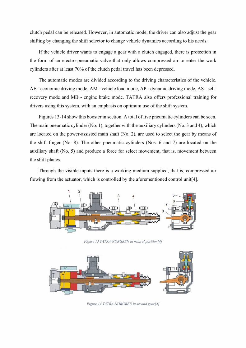
Figures 13-14 show this booster in section. A total of five pneumatic cylinders can be seen.

The main pneumatic cylinder (No. 1), together with the auxiliary cylinders (No. 3 and 4), which

are located on the power-assisted main shaft (No. 2), are used to select the gear by means of

the shift finger (No. 8). The other pneumatic cylinders (Nos. 6 and 7) are located on the

auxiliary shaft (No. 5) and produce a force for select movement, that is, movement between

the shift planes.

Through the visible inputs there is a working medium supplied, that is, compressed air

flowing from the actuator, which is controlled by the aforementioned control unit[4].

Figure 13 TATRA-NORGREN in neutral position[4]

Figure 14 TATRA-NORGREN in second gear[4]

3 Topology Optimization

In the last few years, topology optimization has become an important research area because

of its powerful and efficient algorithms that have been created to enable designers develop

innovative conceptual designs. Specifically, topology optimization has become a powerful area

since its algorithms can be applied in many design problems in different physical disciplines

such as solid mechanics, fluid dynamics, as well as thermal dynamics. Using topology

optimization methods and related algorithms, a designer can generate innovative design ideas

especially in engineering fields. Instead of using trial and error methods in designing

engineering products, designers use different topology optimization methods to generate

conceptual designs (Figure 15). Currently, there are two main topology optimization methods

which are used by most designers namely the Solid Isotropic Material with Penalization

method, otherwise known as SIMP, and the level-set method. These two methods have unique

features and even though each of them can be used to achieve the same goals, they are

fundamentally different. This section will review the characteristic of each method on ANSYS,

show the differences and similarities between them and discuss the advantages and

disadvantages of each method. Even more, both methods will be validated and compared to

other topology optimization software in order to produce the optimized part using additive

manufacturing.

Figure 15 Topology optimization cycle[5]

3.1 Geometry of Model

In topology optimization, it is usually done by creating a geometry that only considers the

constraints of the part ranging from supports to the vacant area that the body can move around

within the assembly. However, since that part has almost no space within the assembly, the

original geometry has been considered in this study with a slight modification for simplicity of

calculations and some fitment issues, where the radius at the tip of the thumb was not perfectly

matching when attaching it into the main assembly, see Figures 16-17.

Figure 16 Original geometry of main shifting thumb [Author]

Figure 17 Modified geometry of main shifting thumb [Author]

3.2 Material of Model

The material assigned is 316 Stainless Steel. As it is the material, which will be used in

additive manufacturing afterwards. The benefits of this material are various. Firstly, we can

consider its widespread availability in the market. Also, it’s one of the leading materials that

has a relatively long history in 3D printing which makes it easier to utilize and design according

the numerous scientific research papers that have been published.

In order to simplify the calculations, nonlinear and thermal strain effects have been

neglected. Such simplifications were considered due to the lack of computing power which

will lead to an undesired time consumed.

Material properties were obtained from a test that has been commissioned on a 3D printed

part at VSB-Technical University of Ostrava laboratories and therefore, a new material

properties were initiated according to the provided test data, see Figures 18-20.

Figure 18 Experimental stress-strain curve of 316 stainless steel [Author]

Figure 19 Modulus of elasticity graph [Author]

0

100

200

300

400

500

600

700

0 0.005 0.01 0.015 0.02

σM

Pa

ε

Static stress-strain curve

y = 183034x - 1.4288

0

50

100

150

200

250

0 0.0002 0.0004 0.0006 0.0008 0.001 0.0012 0.0014

Modulus of Elasticity

Figure 20 Implemented material data into ANSYS [Author]

3.3 Mesh of Model

For calculation simplicity, elements order of the mesh has been considered to be linear.

Linear elements would reduce the quality of the mesh. Therefore, in order to slightly increase

the quality of mesh, Hex Dominant Method has been chosen. Hex dominant method is a method

where it assigns all faces to have hexahedron elements then dragged into the body until it

reaches a point where it is very complex to achieve hexahedron elements. At that point, the

domination of the method ends, and the general meshing rule becomes effective, which is

tetrahedron method, see Figure 21.

Figure 21 Mesh of the main shifting thumb [Author]

3.4 Static Structural Analysis System Setup and Solution

Static structural analysis setup has to be very simple and convenient for topology

optimization program to utilize it with less complexity and that is because of its relation to the

consumed time for solving, where more complex setup would lead to longer solving periods.

Therefore, the analysis settings were configured to have a direct solver and one substep as

shown below, see Figures 22-28.

Figure 22 General overview of applied constraints [Author]

Figure 23 Applied force location [Author]

Figure 24 Applied force values [Author]

Figure 25 Fixed support location [Author]

Figure 26 Cylindrical support location [Author]

Figure 27 Displacement location [Author]

Figure 28 Static structural analysis setting [Author]

Both of Von-Mises Stress, Figure 29, and total deformation, Figure 30 where evaluated as

a reference to the newly developed geometries.

Figure 29 Equivalent (Von-Mises) stress [Author]

Figure 30 Total deformation [Author]

3.5 The SIMP Method on ANSYS Workbench

The simple topology optimization approach makes use of discrete element densities when

generating optimization variables. Therefore, designers are only capable of generating a

staggered grey image of their conceptual design. If the conceptual design is to be manufactured,

the image must go through three post-treatment stages which are identifying the topology

design as the black-and-white image, the smoothening of the structural boundary and the

realization of the parameters. In the early years of topology design field, designers only used

the area as a conceptual idea and they would only make an interpretation of the idea[8].

However, this approximation method was inaccurate and arbitral and hence ineffective. This

limitation was overcome when designers came up with image processing techniques where

grey images were converted into binary maps which could then be processed further to form a

skeleton extraction through boundary smoothening. In other cases, a binary map could be

repaired to remove noisy elements as well as fill the voids before the external boundaries of

the design were constructed.

3.5.1 Advantages and Disadvantages of SIMP Method

The SIMP topology optimization method remains among the most popular methods

because of its conceptual simplicity and computational efficiency. This is mainly because the

method makes use of the isotropic material. As such, the Solid Isotropic Material with

Penalization method allows designers to implement the conceptual designs at a lower

computational cost. Despite the fact that the SIMP method is the most popular of the two

methods, its computational complexity and numerical instability such as the grayscales

elements and checkboard patterns remains to be its major disadvantages. The final optimized

topology must be processed further since it contains a lot of grey elements which make it

blurry[9]. Therefore, most designers find it as not feasible as they will have to do a lot more

before the final production of the design.

3.5.2 Mathematical model

The SIMP method is based on a heuristic relation between (relative) element density 𝑥𝑖

and element Young’s modulus 𝐸𝑖 given by

𝐸𝑖 = 𝐸𝑖(𝑥𝑖) = 𝑥𝑖𝑝𝐸0 , 𝑥𝑖 ∈ [0,1], (1)

where 𝐸0 is the elastic modulus of the solid material, 𝑝 is the penalization power (𝑝 > 1).

A modified SIMP approach is given by

𝐸𝑖 = 𝐸𝑖(𝑥𝑖) = 𝐸𝑚𝑖𝑛 + 𝑥𝑖𝑝(𝐸0 − 𝐸𝑚𝑖𝑛) , 𝑥𝑖 ∈ [0,1],

(2)

where 𝐸𝑚𝑖𝑛 is the elastic modulus of the void material, which is non-zero to avoid singularity

of the finite element stiffness matrix.

The modified SIMP approach offers a number of advantages over the classical SIMP

formulation, including the independency between the minimum values of the materials elastic

modulus and the penalization power[10].

However, topology optimization methods are likely to encounter numerical difficulties

such as mesh dependency, checkerboard patterns, and local minima[11]. In order to mitigate

such issues, researchers have proposed the use of regularization techniques[12]. One of the

most common approaches is the use of density filters[13]. A basic filter density function is

defined as

�̃�𝑖 =∑𝑗∈𝑁𝑖

𝐻𝑖𝑗𝑣𝑗𝑥𝑗

∑𝑗∈𝑁𝑖𝐻𝑖𝑗𝑣𝑗

,

(3)

where 𝑁𝑖 is the neighbourhood of an element 𝑥𝑖 with volume 𝑣𝑖, and 𝐻𝑖𝑗 is a weight factor. The

neighbourhood is defined as:

𝑁𝑖 = {𝑗: 𝑑𝑖𝑠𝑡(𝑖, 𝑗) ≤ 𝑅} ,

(4)

where the operator 𝑑𝑖𝑠𝑡(𝑖, 𝑗) is the distance between the centre of the element 𝑖 and the centre

of element 𝑗, and 𝑅 is the size of the neighbourhood or filter size. The weight factor 𝐻𝑖𝑗 may

be defined as a function of the distance between neighbouring elements, for example

𝐻𝑖𝑗 = 𝑅 − 𝑑𝑖𝑠𝑡(𝑖, 𝑗), (5)

where 𝑗 ∈ 𝑁𝑖. The filtered density �̃�𝑖 defines a modified (physical) density field that is now

incorporated in the topology optimization formulation of the SIMP model as

𝐸𝑖(�̃�𝑖) = 𝐸𝑚𝑖𝑛 + �̃�𝑖𝑝(𝐸0 − 𝐸𝑚𝑖𝑛), �̃�𝑖 ∈ [0,1]. (6)

3.5.3 ANSYS setup and results

3.5.3.1 Setup Overview

The main idea of the topology optimization analysis system is utilizing other analysis

systems, which in our case are the static structural and modal analysis systems, in order to solve

for the main topology optimization analysis system. After the calculation, a new geometry will

be proposed by the software, taking into account the constraints applied in order to achieve the

desired outcome. Such parameters may be a mass constraint, which could be either a constant

limit or a range. Another constraint could be a global or local von-Mises stress constraint,

which ensures that the newly calculated geometry avoids highly stressed areas. Once a newly

designed model has been proposed by the solver, a validation process is executed to evaluate

the whether the new design is valid and good to use or is poorly design and the process has to

be rerun again with modified constraints that help in improving the design. SIMP method has

different constraints that can be applied; thus they are mentioned in Figure 31 as a reference.

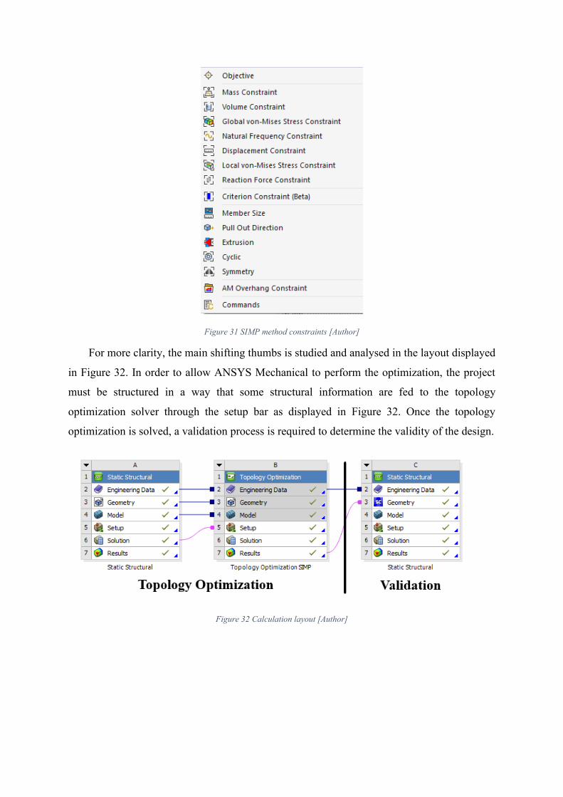
Figure 31 SIMP method constraints [Author]

For more clarity, the main shifting thumbs is studied and analysed in the layout displayed

in Figure 32. In order to allow ANSYS Mechanical to perform the optimization, the project

must be structured in a way that some structural information are fed to the topology

optimization solver through the setup bar as displayed in Figure 32. Once the topology

optimization is solved, a validation process is required to determine the validity of the design.

Figure 32 Calculation layout [Author]

3.5.3.2 Topology Optimization Setup and Results

The Solid Isotropic Material with Penalization method in the topology optimization solver

has its own constraints which makes it distinct from the Level-Set method. Generally, both

methods have mass and natural frequency constraints, but they have different approaches in

the remaining constraints.

For our setup, mass constraint has been assigned and the percentage of mass to retain is

37% of the original mass of the body. Two symmetry constraints where applied as well in both

y-axis and z-axis to retain manufacturability.

Optimization region has been assigned to all faces of the body except for the regions where

there are structural constraints such as loads and supports, as shown in Figures 33-42.


Figure 34 Topology optimization analysis settings SIMP method [Author]

Figure 35 Optimization region settings and method selection [Author]

Since the part is relatively thick, the frequency objective has been switched of in order to

simplify the solution, see Figure 36.

Figure 36 Objective settings [Author]

After several trials with the mass constraint, it has been decided that 63% of mass to be

reduced taking into account the validity of the design (Figure 37).

Figure 37 Mass constraint [Author]

Figure 38 Mass constraint setup [Author]

Two symmetry constraint were applied in both Y-axis and Z-axis to maintain the

manufacturability of the topology optimized part (Figures 39-42).

Figure 39 Symmetry constraint Y-axis [Author]

Figure 40 Symmetry constraint Y-axis setup [Author]

Figure 41 Symmetry constraint X-axis [Author]

Figure 42 Symmetry constraint X-axis setup [Author]

In Figure 43, the solution of this setup took around 22 minutes to solve, which is

convenient for designers to have general overview of the solution without spending a

tremendous amount of time such as the Level-Set method.

Figure 43 Solution information [Author]

As it could be observed from Figure 45 above, the geometry is very rough and proves the

theoretical observations previously mentioned in 3.5.1. Therefore, post-processing is required

to obtain a printable geometry.

Figure 44 Convergence graph [Author]

Figure 45 Final iteration 12 of solution [Author]

3.5.3.3 Smoothing and Validation of the Results

In this chapter, furthermore post processing is being conducted to achieve a printable part.

There are two smoothing steps, one was performed a built it option in ANSYS Mechanical and

the other was performed using SpaceClaim with more smoothing capabilities.

Figure 46 Smoothing in Mechanical ANSYS [Author]

Figure 47 Smoothing in SpaceClaim [Author]

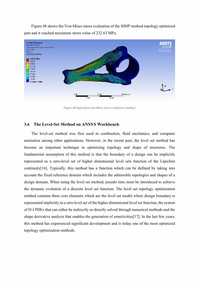
Figure 48 shows the Von-Mises stress evaluation of the SIMP method topology optimized

part and it reached maximum stress value of 232.63 MPa.

Figure 48 Equivalent Von-Mises stress evaluation [Author]

3.6 The Level-Set Method on ANSYS Workbench

The level-set method was first used in combustion, fluid mechanics, and computer

animation among other applications. However, in the recent past, the level set method has

become an important technique in optimizing topology and shape of structures. The

fundamental assumption of this method is that the boundary of a design can be implicitly

represented as a zero-level set of higher dimensional level sets function of the Lipschitz

continuity[16]. Typically, this method has a function which can be defined by taking into

account the fixed reference domain which includes the admissible topologies and shapes of a

design domain. When using the level set method, pseudo time must be introduced to achieve

the dynamic evolution of a discrete level set function. The level set topology optimization

method contains three core elements which are the level set model where design boundary is

represented implicitly as a zero level set of the higher dimensional level set function, the system

of H-J PDEs that can either be indirectly or directly solved through numerical methods and the

shape derivative analysis that enables the generation of sensitivities[17]. In the last few years,

this method has experienced significant development and is today one of the most optimized

topology optimization methods.

3.6.1 Advantages and Disadvantages of Level Set Method

The level set topology optimization method is a relatively new method in the area of

conceptual designs. It is a versatile yet a simple method that is used to track the interfaces’

evolution. Since its first introduction, level set method has gained the attention of many

researchers because unlike the other traditional topology optimization methods, it is more

effective and direct when dealing with most structural optimization problems. The method

allows designers to come up with shapes with distinct interfaces. As such, this method allows

designers to solve design problems with string interfacial phenomena while at the same time

avoiding the ambiguous grey-scale intermediate densities that surround the design boundary

[18]. When using this method, it is possible to develop smooth boundaries which is an

important characteristic of design problems that require more accurate response and interface.

Through the level set topology method, it is possible to generate a meaningful physical solution

using the Hamilton-Jacobi PDEs. The main disadvantage which is associated with the level set

method is the Courant-Friedrichs-Lewy condition. It is also associated with difficulty in how

finite difference techniques are used.

3.6.2 Mathematical model

The compliance function in the Level-Set method relies on the response type or constraint.

The static structural analysis supports the combination of force-based and displacement-based

loading as well as thermal loading. The compliance function can be described as following

𝐽(Ω) =1

2[∫ 𝐴(𝑒(𝑢) − 𝑒𝑡ℎ): 𝑒𝑡ℎ𝑑𝑥

−

Ω

+ ∫ 𝑓 ∗ 𝑢𝑑𝑥

−

Ω

+ ∫ 𝑔 ∗ 𝑢𝑑𝑠

−

Γ𝑁

+ ∫ 𝜆𝑢 ∗ 𝑢0𝑑𝑠

−

Γ𝑢

]

= [−1

2∫ 𝐴(𝑒(𝑢) − 𝑒𝑡ℎ): (𝑒(𝑢) − 𝑒𝑡ℎ)𝑑𝑥

−

Ω

+ ∫ 𝑓 ∗ 𝑢𝑑𝑥

−

Ω

+ ∫ 𝑔 ∗ 𝑢𝑑𝑠

−

Γ𝑁

]

(7)

where

𝑒(𝑢) =1

2(∇𝑢 + (∇𝑢)𝑡) , is the total strain vector

𝑒𝑡ℎ , the thermal strain vector.

(𝑒(𝑢) − 𝑒𝑡ℎ) , is the elastic strain vector.

𝜎(𝑢) = 𝐴(𝑒(𝑢) − 𝑒𝑡ℎ) , is the stress vector.

(𝑓, 𝑔) , are the external loads.

(𝜆𝑢, 𝑢0) , are the reaction force and the prescribed displacement.

These formulas are equivalent and are based on the potential energy. The compliance is a

self-adjoint response meaning that no adjoint problem needs to be solved. The compliance is

always computed over the whole model[14].

Displacement-based Criterion

Context for displacement-based response:

• For a singular node selection, the response = 𝐽(Ω) = |𝑢𝑘𝑖 | (𝑖𝑡ℎ node, 𝑘-axis). Upper

limit can be defined for each direction.

• For multiple node selection, the response = 𝐽(Ω) =1

|𝐵|∫ |𝑢𝑘|

−

𝐵𝑑𝑠 (the average of the

absolute displacement along the 𝑘-axis).

Reaction Force Criterion

• For a singular node selection, the response = 𝐽(Ω) = |𝜆𝑘𝑖 | (𝜆 = 𝜎𝑛) (𝑖𝑡ℎ node, 𝑘-

axis). Upper limit can be defined for each direction.

• For multiple node selection, the response = 𝐽(Ω) = ∫ |𝜆𝑘(𝑥)|−

𝐵𝑑𝑠 (𝜆 = 𝜎𝑛) (the

absolute RF along the 𝑘-axis) [14].

3.6.3 ANSYS setup and results

3.6.3.1 Setup Overview

The setup of the Level-Set method differs from SIMP method in minor areas but in general

they almost have similar setups. The main difference in setup is constraints applied to achieve

a desired outcome. Such parameters may be a mass constraint, which could be either a constant

limit or a range. Figure 49 shows the constraints that can be applied which can be noticed that

it is slightly different from SIMP method constraints list.

Figure 49 Level-Set method constraints [Author]

Project layout (Figure 50) is similar to the layout mentioned in 3.5.3.1 Figure 32, but as

for the Level-Set, the only thing that is different is the naming of the topology optimization

solver box.

Figure 50 Calculation layout [Author]

3.6.3.2 Topology Optimization Setup and Results

The Level-Set method in the topology optimization solver has its own constraints which

makes it distinct from the SIMP method. Generally, both methods have mass and natural

frequency constraints but they have different approaches in the remaining constraints.

For our setup, only mass constraint has been assigned and the percentage of mass to retain

is 37% of the original mass of the body. Also, in contrast to the SIMP method, exclusion

thickness is accounted for in this method which allows to avoid additional constraints in the

setup.

Optimization region has been assigned to all faces of the body except for the regions where

there are structural constraints such as loads and supports, as shown in Figure 51-52.


Figure 52 Topology optimization analysis settings Level-set method [Author]

As shown in Figure 53, the exclusion thickness has been set to 5 mm in order to prevent

extremely thin walls which would be structurally invalid.

Figure 53 Optimization region settings and method selection [Author]

Also, for the same justification for the SIMP method, frequency criterion has been

neglected due to the geometry of the design (Figure 54).

Figure 54 Objective settings [Author]

Figure 55-56 show the mass constraint which requires the solver to retain 37% of the body

mass.

Figure 55 Mass constraint [Author]

Figure 56 Mass constraint setup [Author]

In Figure 57, the solution of this setup took around 7 hours to compute, which is not

convenient for designers but the results are more valuable as less work required to finalize the

geometry for production. Convergence graph of the objective response is displayed in Figure

58.

Figure 57 Solution information [Author]

Figure 58 Convergence graph [Author]

Figure 59 shows the 3rd iteration of the solver where it can be observed how the part

undergoes topology optimization process.

Figure 59 Iteration 3 of solution [Author]

It could be observed from Figure 60 that the Level-Set method produces smoother

geometry and that is conducted by avoiding grey-scale intermediate densities 3.6.1.

Figure 60 Final iteration 22 of solution [Author]

3.6.3.3 Smoothing and Validation of the Results

Moving to the validation process, the body gets roughly smoothed before transferring to

SpaceClaim software in order to further refine it, then it is transferred to the design validation

system. Move limit is set to 1 for rough smoothing which was done using Mechanical ANSYS

system (Figure 61) before transferring it to SpaceClaim software (Figure 62).

Figure 61 Smoothing in Mechanical ANSYS [Author]

Figure 62 Smoothed geometry in SpaceClaim [Author]

Final evaluation of the smoothed Level-Set method topology optimized part is displayed

in Figure 63 where the maximum equivalent Von-Mises stress is evaluated at 285.66 MPa.

Figure 63 Equivalent Von-Mises stress evaluation [Author]

3.7 Other Approaches

For assurance of the design validity, another software has been considered. ANSYS

Discovery Live, a newly built software, which is tremendously easier and quicker in solving

compared to ANSYS Workbench. Discovery Live relies on a different approach where mesh

of the geometry, which consumes a large amount of time, is not required to be implemented by

the user. Even more, the solution time compared to Workbench to develop the new design is

significantly lower where it took around five minutes.

This software is highly recommended to have general understanding of what shapes are

expected to be developed. Such solving speed allowed to investigate variants of volume

reduction. The method that the solver utilizes is unknown therefore is has been discussed

separately in a single subchapter. In the following Figure 64-69, Discovery Live solution will

be discussed. There is no function in Discovery Live making possible to get symmetric

topology optimised geometry, which is why the force was applied on two facets, see Figure 64.

Figure 64 ANSYS Discovery Live structural constraints [Author]

Table 6 displays the parameters considered in the calculations with several variants of

volume reduction.

Table 6 Topology optimization analysis settings [Author].

Parameter Set Value

Analysis Type Topology optimization

Target Structural

Goal Maximize stiffness

Volume Reduction – constraint 60% - 65% - 63% - 64%

Protection Distance - constraint 3 mm

Equivalent Von-Misses Stress evaluations of different volume reductions are ordered

respectively in Figure 65-68. It appears from the figures that the resulting geometry is similar

to ANSYS Workbench Level-Set method topology optimization.

Figure 65 Topology optimization result (volume reduction 60%) [Author]




Table 7 displays the Von-Mises stress values of each trial. From an engineering intuition

perspective, the first trial was considered to be too robust. Also, the second trial was considered

to be too weak. The third and fourth trials were very similar, therefore, the stress values were

compared and thus the third trial was lower and considered for the upcoming post processing

an analysis (Figure 69).

Table 7 Table of trials [Author]

Trial Volume Reduction Von-Mises Stress (MPa)

1 60% 233.43

2 65% 255.86

3 63% 232.25

4 64% 242.20

Figure 69 Final geometry (trial 3) [Author]

For validation purposes, the geometry has been modified where only one half was

considered for mirror operation which assures symmetry of the body. Symmetry was

considered to avoid structural defects when uniform force is applied. Then, the geometry has

been smoothed furthermore using SpaceClaim to obtain a smoother surface when 3D printed.

Furthermore, an elliptical support has been added to the tip of the part where force is being

applied to ensure the stiffness of the model (Figure 70). In ANSYS Workbench, quality of

meshing was dependent on the Hex Dominant method and quadratic element order which was

limited due to the license restrictions.

Figure 70 Symmetry and smoothing modifications [Author]

Figure 71 shows the equivalent Von-Misses stress values of the newly designed part which

is evaluated with maximum stress of 214.24 MPa. Such value is highly acceptable considering

a 63% mass reduction of the original geometry which was evaluated at 221.53 MPa (Figure

29).

Figure 71 Validation of trial 3 with 63% reduction [Author]

Elliptical support

3.8 Selection of Printed Part

The SIMP topology optimization method makes use of element or the nodal densities when

generating optimization variables. This method is thus sometimes referred to as the element-

based method which can freely generate changes in a topology fast while ensuring that the

design is stable. On the other hand, the level set topology optimization method defines the

domain of a material using a positive set field as well as the structural boundary of a design

using the zero-value set contour[19]. The level set method is thus sometimes referred to as the

boundary based structural evolution method. The level set method uses smooth and clear-cut

representations of the boundary. However, during implementation of this method, the boundary

elements are represented using the approximate Heaviside projects as well as what is passed

into a finite element model which is actually blurred.

The level set topology optimization method has emerged as one of the most powerful

methodologies for topology and shape optimization of structures. This method uses the concept

of representing the structural boundary implicitly as a zero-level set of the higher-dimensional

scalar function that is mathematically defined. This method has a lot of features as compared

to the SIMP method that is well suited for optimization of topologies and structures. Besides

its application on topological optimization of designs and structures, it can also be used in the

computational design area of mechanical materials and designs. On the other hand, the SIMP

method helps designers to obtain a temporary optimized topology or structure which must be

processed further before the final production takes place.

After completing several topology optimization trials, and including the discussion

aforementioned that arguably favours the Level-Set method. It has been decided that the

Discovery Live topology optimized resulted part is the one that the paper will continue its

course with.

4 Additive Manufacturing

4.1 Types of Additive Manufacturing Technologies

There are several technologies for Additive Manufacturing. Starting with the most

common and cheaper option which is Fused Deposition Modelling (FDM). This technology is

based on material extrusion by melting the filament on the heated in order to form the object.

Another common technology that’s used for more accurate smaller prints is Stereolithography

(SLA) where it uses laser light as hardening component to the pool of epoxy resin and making

the part afterwards. Also, there is another common technology which is Selective Laser

Sintering (SLS). This technology is based on powder bed fusion combined with laser beams to

make the part. Aforementioned technologies are based on thermoplastic materials.

Another field of additive manufacturing deals with metal alloys and depends on the

weldability to be more precise. Such technologies are Laser Melting Deposition (LMD) where

this technology welds material through a moving nozzle to finally formulate the desired shape.

Our focus in this thesis is the Selective Laser Melting (SLM) technology which will be used in

order to print the topology optimized part.

4.2 Selective Laser Melting (SLM)

Selective Laser Melting technology (Figure 72) has several synonyms which are Direct

Metal Laser Sintering (DMLS), Laser Metal Fusion (LMF), Direct Metal Printing (DMP),

Laser Beam Melting (LBM) and Direct Metal Laser Melting. This technology relies on the

powder bed fusion using laser beams. A brief illustration is displayed in Figure 73.

Figure 72 Stainless steel square hollow section (SHS) member built using SLM[15]

Figure 73 Selective Laser Melting process[21]

4.3 Renishaw AM 400 Additive Manufacturing System

The AM 400 system offers a 400 W focussed at 70 µm laser beam which allows for higher

melting temperatures. It has a flexible and rapid material changeover with low argon

consumption. It also allows for the build to be removed with enhanced safety.

Renishaw’s patented class leading inert atmosphere generation works by first creating a

vacuum before back filling with high purity argon gas. This method ensures a high quality

build environment as well as minimal argon usage for atmosphere generation, suitable for all

qualified metals including titanium and aluminium. Gas consumption is further minimised by

the use of a sealed and welded chamber.

Figure 74 AM 400 additive manufacturing system[20]

4.4 Materials Used for 3D Printing

Renishaw supplies a range of high quality metal powders including Ti6Al4V ELI,

AlSi10Mg, Stainless Steel 316L ( SS 316L-0407 ) , tool steels (such as Maraging Steel 300),

nickel alloys and cobalt chromium alloy.

For this diploma, it has been considered to design the part using Stainless Steel 316L. Such

decision has been made in order to maintain cost of production. Another material possibility

would be Maraging Steel 300 with heat treatment. Such possibility would be taken into

consideration if cost of production is flexible and the designed part’s robustness was not

sufficient for the application.

Additive manufacturing material properties of Stainless Steel 316L are different than the

conventional Stainless Steel material properties and thus they are defined in Table 8.

Table 8 Mechanical properties of SS 316L-040[22]

4.5 ANSYS Printing Setup and Thermal Analysis

The additive manufacturing setup was accomplished using ANSYS SpaceClaim. The

software offers an orientation map feature (Figure 75) where it simulates all possible angles

and calculate build time, distortion tendency, and supports. Furthermore, 3D printing was made

using SLM (Selective Laser Melting) machine manufactured by RENISHAW model AM400.

Figure 75 Orientation map [Author]

Figure 76 Selected orientation [Author]

After the selection of the appropriate orientation (Figure 76), the model then undergoes an

additive manufacturing thermal analysis to simulate the printing process and predict structural

defects such as deformation due to shrinkage during cooling time. The printing simulation

parameters that will be used to thermally evaluate the process are prescribed in Table 9.

Table 9 3D Printing parameters[25]

3D Printer: Renishaw AM400

Powder description: SS Powder AISI 316L (DIN 1.4404)

Powder Particle Size: 15–45 µm

Layer Thickness: 50 µm

Focus Size: 70 µm

Print Strategies: Chessboard, see Figure 77

Border Power: 110 W

Border Exposure Time: 100 µs

Border Point Distance: 20 µm

Hatches Power: 200 W

Hatches Exposure Time: 80 µs

Hatches Point Distance: 60 µm

Jump speed: 5000 mm·s-1

Dosing time: 7 s

Melting range: 1371 °C to 1399 °C

Concentration of Oxygen: < 0,1 % O2

Inert Gas: Argon

Purity: 5.0 (99.998 %)

Figure 77 Chessboard print strategy[26]

Using ANSYS Additive Manufacturing Wizard, the following project setup would

automatically generate (Figure 78). AM thermal analysis meshing is displayed in Figure 79,

also AM thermal analysis results are shown in Figure 80 which confirms that the effective

thermal stress proportionally related to the increase of layer height from bed surface[23].

Figure 78 Additive Manufacturing thermal analysis setup [Author]

Figure 79 AM thermal analysis mesh [Author]

Figure 80 AM thermal analysis [Author]

Figure 81 AM Structural analysis [Author]

Figure 81 shows an unacceptable result and such issue arise because of using Cartesian

mesh. Therefore, a subsequent finite element analysis (submodeling) is required to obtain finer

and more accurate results by selecting more suitable mesh. Such process was performed with

suppressed base plate and ignored nonlinear effect as well as initial strain.

Figure 82 Standalone structural analysis [Author]

After obtaining the evaluation of the simulated printing process in Figure 82, theoretical

results are then verified by performing the printing process and perform a deformation test

during cutting the part from its base plate in the chapter 4.7.

4.6 Printing Results

Below figures briefly illustrates the process of the printing cycle of the topology optimised

part. At first, the part was printed on RENISHAW AM400 machine using Stainless Steel 316L

as a material. After the completion of printing process, excess powder material was then safely

removed for recycling into future jobs. Then, the printed part goes through cutting from base

plate process which was investigated to observe if any deformation occurs in the printed part.

Figure 83 shows the printing process of the desired part. Figure 84-86 show the removal

process of powder metal then clean-up of printing part.

Figure 83 Part printing under process [Author]

Figure 84 Residual powder material removal [Author]

Figure 85 Printed part with supports and base plate

[Author]

4.7 Testing

Testing was performed using Digital Image Correlation (DIC) which is a method of

measurement where no contact to the investigated part is required. This method utilizes optical

testers which measure deformation, strain and vibration on any part.

Due to time constraints, fatigue testing was not possible and only static-deformation

testing was considered. The DIC testing goal is to investigate the deformation of the part and

compare it to the obtained calculated deformation.

4.7.1 Setup

The software used in analysing the data is Mercury RT which is capable of three-

dimensional measurements. Two high accuracy cameras where fixed in front of the

investigated part during the cutting process. The cameras record the deformation of the part

once the cutting process has begun. With the capabilities of the software, colour coded

deformation is then produced to compare it with the theoretical deformation data. Figure 86

shows the setup for recording the part’s deformation while being cut in Figure 87.

Figure 86 Cameras used for testing and setup [Author]

Figure 87 Setup during cutting process [Author]

After the cutting process, pictures were taken from top and bottom side for visual

inspection in Figure 88.

Figure 88 Top and bottom sides after cutting [Author]

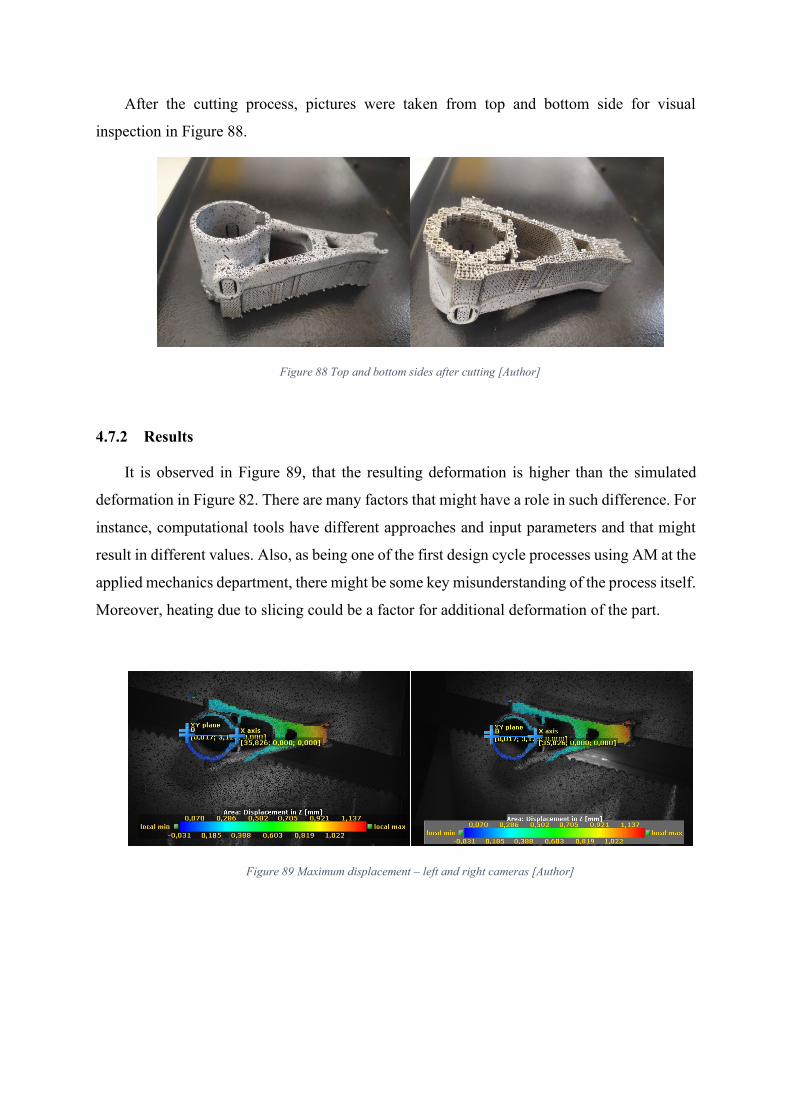
4.7.2 Results

It is observed in Figure 89, that the resulting deformation is higher than the simulated

deformation in Figure 82. There are many factors that might have a role in such difference. For

instance, computational tools have different approaches and input parameters and that might

result in different values. Also, as being one of the first design cycle processes using AM at the

applied mechanics department, there might be some key misunderstanding of the process itself.

Moreover, heating due to slicing could be a factor for additional deformation of the part.

Figure 89 Maximum displacement – left and right cameras [Author]

5 Conclusion

The main purpose of this study is to incorporate new technologies into design and

manufacturing. TATRA TRUCKS a.s. has a well-known history in automobile industry, and

as being in the field of customized trucks manufacturing, it is crucial to accommodate new

design solutions and manufacturing technologies that will allow TATRA to achieve more

robust yet light weight trucks and achieve more manoeuvrability which has been already

reached using the backbone tube. As part of the continuous support in the research and

development department, a newly designed gearshift booster is further investigated for more

developmental aspect. The shifting thumb part has a great potential to be utilized by topology

optimization and additive manufacturing for being a small part that continuously endures high

loads and being a very crucial part to maintain the safety of the driver.

The part has gone through several steps, starting from design optimization, where the main

shifting thumb has been slightly modified to snuggly fit into the assembly. Then it was topology

optimized using several methods and software. Three variants resulted from such process

which were then structurally evaluated, and one variant was chosen. The variant chosen was

the one produced by ANSYS Discovery Live and the two remaining where used as references

to what are the possibilities that different software and methods can achieve. After the design

part was completed, additive manufacturing using selective laser melting technology was

considered. Thermal additive manufacturing simulation was performed to estimate the

deformation of the part after cutting. After printing the part in stainless steel using Renishaw

AM400, testing has been conducted using Digital Image Correlation (DIC) to observe the

deformation of the part while releasing it from the base plate and compare it to the simulated

values.

The main comparison is in deformation of the part after cutting which is slightly different

than the simulations obtained earlier in the course of the diploma thesis. Such difference has

many factors that reflect on the observation. The factor that can be easily pointed out is the

material properties that were implemented into the simulation process where ANSYS material

library was the source of the material properties assigned. Material properties of the printed

part differ from the material properties available in the library. Even more, meshing of the

bodies might have a significant impact since the calculations where constrained to limited

number of elements to run the calculations, and that is due to the student license capabilities.

As being one of the first experiments using topology optimization tools alongside with

additive manufacturing using stainless steel (SS 316 L), the process might have encountered

some flows which resulted in slight deformation difference between theoretical and

experimental data. There are many aspects in such difference, one of which is the software

simulation accuracy where the input data may have been determined correctly but due to

software coding, different results were obtained. This experiment gives the chance to analyse

the accuracy of the simulation in future studies.

There are some challenges that constraint the advancement of additive manufacturing to

be rapidly implemented into the manufacturing eco system. Cost, to begin with, is one of the

challenges where additive manufacturing technology is rapidly evolving and new technologies

are developed to enable some manufacturing features where that affects the cost of making a

product. The current manufacturing capabilities such as casting are very rapid and efficient

which makes it difficult for additive manufacturing technologies to join the race. Another

challenge would be the manufacturing process variability and limitation where each additive

manufacturing machine method might produce different results using the same 3D CAD file.

Furthermore, the calibration of each equipment varies from each producer which makes it

unstandardized process. Also, material properties encounter the same issue. Design and

verification of a structure can be introduced as a challenge as well, where anisotropy, geometric

imperfections and residual stresses are always higher in additive manufacturing compared to

conventional material[24].

The importance of this experiment relies on being one of several additive manufacturing

experiments at the department of applied mechanics which allows the department to have a

general overview and finer analysis of the process in future studies. It is also important to make

sure that the computational tools are usable for similar cases. This experiment has been very

enlightening the industry of additive manufacturing and we look forward to continuing

cooperation with companies and institutions.

ACKNOWLEDGMENTS

This research was supported by the Technology Agency of the Czech Republic in the

frame of the project TN01000024 National Competence Center-Cybernetics and Artificial

Intelligence and by the project Innovative and additive manufacturing technology—new

technological solutions for 3D printing of metals and composite materials, reg. no.

CZ.02.1.01/0.0/17_049/0008407 financed by Structural Funds of Europe Union.

I would like to extend my gratitude and appreciation to both of, my advisor prof. Ing.

Radim Halama, Ph.D. and Mr. Miroslav Krizek from TATRA Truck a.s., for their continuous

support and guidance, where they never hesitated with providing the support needed to

accomplish my diploma thesis.

6 Bibliography

[1] MACHÁLEK FILIP. Proporsal for Modifying of the Power Shift of the Truck Manual

Gearbox. Ostrava : VŠB – Technical University of Ostrava, Faculty of Mechanical

Engineering, Department of Production Machines and Design, 2018, 69 s. Thesis

head: Ing. Ladislav Hrabec, Ph.D.

[2] TATRA concept: TATRA.cz. TATRA WILL GET YOU FURTHER [online].

Available from: https://www.tatra.cz/proc-tatru/technicka-koncepce-tatra/tatrovacka-

koncepce/

[3] TATRA transmissions: Tatratrucks.com. TATRA TAKES YOU FURTHER [online].

Available from: https://www.tatratrucks.com/why-tatra/tatra-vehicle-design/tatra-

transmissions/

[4] Training manual 14TS210N. Kopřivnice, 2011.

[5] Engineering Simulation Consultancy, Software & Training [online]. Available from:

https://wildeanalysis.co.uk/wp-content/uploads/2018/02/ANSYS-additive-

manufacturing-simulation-process.png

[6] Workshop manual for trucks T815, TATRA, 1989.

[7] Norgren spare parts list. Kopřivnice.

[8] Shojaee, S., and M. Mohammadian. "Structural Topology Optimization Using An

Enhanced Level Set Method". Scientia Iranica, vol 19, no. 5, 2012, pp. 1157-1167.

Elsevier BV, doi:10.1016/j.scient.2012.06.024.

[9] Li, Yilun et al. "A Methodology For Topology Optimization Based On Level Set

Method And Its Application To Piezoelectric Energy Harvester Design".

International Journal of Applied Electromagnetics and Mechanics, vol 59, no. 1,

2019, pp. 79-85. IOS Press, doi:10.3233/jae-171098.

[10] Sigmund O. “Morphology-based black and white filters for topology optimization”.

Struct Multidiscip Optim, vol 33, 2007, pp. 401–424.

[11] Bendsøe MP, Sigmund O. “Topology optimization: theory, method and

applications”. Springer, 2007.

[12] Sigmund O, Peterson J. “Numerical instabilities in topology optimization: a survey

on procedures dealing with checkerboards, mesh-dependencies and local minima”.

Struct Optim vol 16, 1998, pp. 68–75.

https://www.tatra.cz/proc-tatru/technicka-koncepce-tatra/tatrovacka-koncepce/

https://www.tatra.cz/proc-tatru/technicka-koncepce-tatra/tatrovacka-koncepce/

https://www.tatratrucks.com/why-tatra/tatra-vehicle-design/tatra-transmissions/

https://www.tatratrucks.com/why-tatra/tatra-vehicle-design/tatra-transmissions/

[13] Bruns TE, Tortorelli DA. “Topology optimization of non-linear elastic structures

and compliant mechanisms”. Comput Methods Appl Mech Eng vol 190, 2001, no.

26–27, pp 3443–3459.

[14] - ANSYS Help. - ANSYS Help [online]. Available from:

https://ansyshelp.ansys.com/Account/Login?ReturnUrl=%2FViews%2FSecured%2Fc

orp%2Fv195%2Fwb_sim%2Fds_topo_opt_level_set

[15] Jared BH, Aguilo MA, Beghini LL, Boyce BL, Clark BW, Cook A, et al. “Additive

manufacturing: toward holistic design”. Scr Mater. 2017, vol. 135, pp 141–7.

[16] Luo, Zhen. "A Short Survey: Topological Shape Optimization Of Structures Using

Level Set Methods". Journal Of Applied Mechanical Engineering, vol 02, no. 03,

2013. OMICS Publishing Group, doi:10.4172/2168-9873.1000123.

[17] Wang, Yaguang, and Zhan Kang. "Structural Shape And Topology Optimization Of

Cast Parts Using Level Set Method". International Journal For Numerical Methods

In Engineering, vol 111, no. 13, 2017, pp. 1252-1273. Wiley, doi:10.1002/nme.5503.

[18] Rozvany, G.I.N. "Aims, Scope, Methods, History And Unified Terminology Of

Computer-Aided Topology Optimization In Structural Mechanics". Structural And

Multidisciplinary Optimization, vol 21, no. 2, 2001, pp. 90-108. Springer Science And

Business Media LLC, doi:10.1007/s001580050174.

[19] Liu, Jikai, and Yongsheng Ma. "A Survey Of Manufacturing Oriented Topology

Optimization Methods". Advances In Engineering Software, vol 100, 2016, pp. 161-

175. Elsevier BV, doi:10.1016/j.advengsoft.2016.07.017.

[20] AM 400. Brochure [online]. Copyright © [cit. 29.04.2020]. Available

from: https://www.renishaw.com/en/am-400--35456

[21] Rasch, M.: Konstruktive Gestaltung einer Forschungsanlage für das

Laserstrahlschmelzen von Metallen aus dem Pulverbett. Master’s thesis, Institute of

Photonic Technologies, Friedrich-Alexander-Universität Erlangen-Nürnberg

[22] Renishaw Plc. Data Sheets—Additive Manufacturing. Renishaw, 2019, UK.

Available online: https://www.renishaw.com/en/data-sheets-additive-manufacturing--

17862.

[23] Peiying B, Xiaodong S, and Jingli D. “Finite Element Analysis of Thermal Stress

and Thermal Deformation in Typical Part during SLM”. 2019.

[24] C. Buchanan, L. Gardner. “Metal 3D printing in construction: A review of methods,

research, applications, opportunities and challenges”. 2018.

https://www.renishaw.com/en/am-400--35456

https://www.renishaw.com/en/data-sheets-additive-manufacturing--17862

https://www.renishaw.com/en/data-sheets-additive-manufacturing--17862

[25] Halama, R., Pagáč, M., Paška, Z., Pavlíček, P., Chen, X. “Ratcheting Behaviour of

3D Printed and Conventionally Produced SS316L Material”. Proceedings of the

ASME 2019 Pressure Vessels & Piping Conference PVP2019 July 14-19, 2019, San

Antonio, TX, USA, paper number PVP2019- 93384.

[26] Jamasp J., Eric B., Thibaud A. and Re´my G. “On the effect of scanning strategies in

the selective laser melting process”. Virtual and Physical Prototyping, vol. 5, no. 2,

June 2010, pp. 99-109.

Optimalizace vybrané části posilovače řazení vozů TATRA pro ...

Documents

Transcript of Optimalizace vybrané části posilovače řazení vozů TATRA pro ...