Optimal Transport Approach for Probabilistic Robustness Analysis of F-16 Controllers
27
1 A Probabilistic Method for Nonlinear Robustness Analysis of F-16 Controllers Abhishek Halder * , Kooktae Lee, and Raktim Bhattacharya Abstract This paper presents a new framework for controller robustness verification with respect to F-16 aircraft’s closed-loop performance in longitudinal flight. We compare the state regulation performance of a linear quadratic regulator (LQR) and a gain-scheduled linear quadratic regulator (gsLQR), applied to nonlinear open-loop dynamics of F-16, in presence of stochastic initial condition and parametric uncertainties, as well as actuator disturbance. We show that, in presence of initial condition uncertain- ties alone, both LQR and gsLQR have comparable immediate and asymptotic performances, but the gsLQR exhibits better transient performance at intermediate times. This remains true in the presence of additional actuator disturbance. Also, gsLQR is shown to be more robust than LQR, against parametric uncertainties. The probabilistic framework proposed here, leverages transfer operator based density computation in exact arithmetic and introduces optimal transport theoretic performance validation and verification (V&V) for nonlinear dynamical systems. Numerical results from our proposed method, are in unison with Monte Carlo simulations. Index Terms Probabilistic robustness, uncertainty propagation, transfer operator, optimal transport. I. I NTRODUCTION In recent times, the notion of probabilistic robustness [2]–[8], has emerged as an attractive alternative to classical worst-case robust control framework. There are two key driving factors * Corresponding author. This research was supported by NSF grant CSR-1016299 with Dr. Helen Gill as the program manager. Some preliminary results were presented [1] in American Control Conference, 2013. The authors are with the Department of Aerospace Engineering, Texas A&M University, College Station, TX 77843-3141, USA. e-mail: {ahalder,animodor,raktim}@tamu.edu February 4, 2014 DRAFT arXiv:1402.0147v1 [cs.SY] 2 Feb 2014
Transcript of Optimal Transport Approach for Probabilistic Robustness Analysis of F-16 Controllers
1
A Probabilistic Method for Nonlinear
Robustness Analysis of F-16 Controllers
Abhishek Halderlowast Kooktae Lee and Raktim Bhattacharya
Abstract
This paper presents a new framework for controller robustness verification with respect to F-16
aircraftrsquos closed-loop performance in longitudinal flight We compare the state regulation performance
of a linear quadratic regulator (LQR) and a gain-scheduled linear quadratic regulator (gsLQR) applied
to nonlinear open-loop dynamics of F-16 in presence of stochastic initial condition and parametric
uncertainties as well as actuator disturbance We show that in presence of initial condition uncertain-
ties alone both LQR and gsLQR have comparable immediate and asymptotic performances but the
gsLQR exhibits better transient performance at intermediate times This remains true in the presence of
additional actuator disturbance Also gsLQR is shown to be more robust than LQR against parametric
uncertainties The probabilistic framework proposed here leverages transfer operator based density
computation in exact arithmetic and introduces optimal transport theoretic performance validation and
verification (VampV) for nonlinear dynamical systems Numerical results from our proposed method are
in unison with Monte Carlo simulations
Index Terms
Probabilistic robustness uncertainty propagation transfer operator optimal transport
I INTRODUCTION
In recent times the notion of probabilistic robustness [2]ndash[8] has emerged as an attractive
alternative to classical worst-case robust control framework There are two key driving factors
lowast Corresponding author This research was supported by NSF grant CSR-1016299 with Dr Helen Gill as the program manager
Some preliminary results were presented [1] in American Control Conference 2013
The authors are with the Department of Aerospace Engineering Texas AampM University College Station TX 77843-3141
USA e-mail ahalderanimodorraktimtamuedu
February 4 2014 DRAFT
arX
iv1
402
0147
v1 [
csS
Y]
2 F
eb 2
014
2
behind this development First it is well-known [8] that the deterministic modeling of uncertainty
in the worst-case framework leads to conservative performance guarantees In particular from a
probabilistic viewpoint classical robustness margins can be expanded significantly while keeping
the risk level acceptably small [9]ndash[11] Second the classical robustness formulation often
leads to problems with enormous computational complexity [12]ndash[14] and in practice relies
on relaxation techniques for solution
Probabilistic robustness formulation offers a promising alternative to address these challenges
Instead of the interval-valued structured uncertainty descriptions it adopts a risk-aware per-
spective to analyze robustness and hence explicitly accounts the distributional information
associated with unstructured uncertainty Furthermore significant progress have been made in the
design and analysis of randomized algorithms [7] [15] for computations related to probabilistic
robustness These recent developments are providing impetus to a transition from ldquoworst-caserdquo
to ldquodistributional robustnessrdquo [16] [17]
A Computational challenges in distributional robustness
In order to fully leverage the potential of distributional robustness the associated computation
must be scalable and of high accuracy However numerical implementation of most probabilistic
methods rely on Monte Carlo like realization-based algorithms leading to high computational
cost for implementing them to nonlinear systems In particular the accuracy of robustness compu-
tation depends on the numerical accuracy of histogram-based (piecewise constant) approximation
of the probability density function (PDF) that evolves spatio-temporally over the joint state and
parameter space under the action of closed-loop nonlinear dynamics Nonlinearities at trajectory
level cause non-Gaussianity at PDF level even when the initial uncertainty is Gaussian Thus in
Monte Carlo approach at any given time a high-dimensional nonlinear system requires a dense
grid to sufficiently resolve the non-Gaussian PDF incurring the lsquocurse of dimensionalityrsquo [18]
This is a serious bottleneck in applications like flight control software certification [19]
where the closed loop dynamics is nonlinear and linear robustness analysis supported with
Monte Carlo remains the state-of-the art Lack of nonlinear robustness analysis tools coupled
with the increasing complexity of flight control algorithms have caused loss of several FA-
18 aircrafts due to nonlinear ldquofalling leaf moderdquo [20] that went undetectable [21] by linear
robustness analysis algorithms On the other hand accuracy of sum-of-squares optimization-
February 4 2014 DRAFT
3
based deterministic nonlinear robustness analysis [19] [20] depends on the quality of semi-
algebraic approximation and is still computationally expensive for large-scale nonlinear systems
Thus there is a need for controller robustness verification methods that does not make any
structural assumption on nonlinearity and allows scalable computation while accommodating
stochastic uncertainty
B Contributions of this paper
1) PDF computation in exact arithmetic Building on our earlier work [22] [23] we show
that stochastic initial condition and parametric uncertainties can be propagated through the
closed-loop nonlinear dynamics in exact arithmetic This is achieved by leveraging the fact
that the transfer operator governing the evolution of joint densities is an infinite-dimensional
linear operator even though the underlying finite-dimensional closed-loop dynamics is nonlinear
Hence we directly solve the linear transfer operator equation subject to the nonlinear dynamics
This crucial step distinguishes the present work from other methods for probabilistic robustness
computation by explicitly using the exact values of the joint PDF instead of empirical estimates of
it Thus from a statistical perspective the robustness verification method proposed in this paper
is an ensemble formulation as opposed to the sample formulations available in the literature [7]
[13]
2) Probabilistic robustness as optimal transport distance on information space Based on
Monge-Kantorovich optimal transport [24] [25] we propose a novel framework for computing
probabilistic robustness as the ldquodistancerdquo on information space In this formulation we measure
robustness as the minimum effort required to transport the probability mass from instantaneous
joint state PDF to a reference state PDF For comparing regulation performance of controllers with
stochastic initial conditions the reference state PDF is Dirac distribution at trim If in addition
parametric uncertainties are present then the optimal transport takes place on the extended state
space with the reference PDF being a degenerate distribution at trim value of states We show
that the optimal transport computation is meshless non-parametric and computationally efficient
We demonstrate that the proposed framework provides an intuitive understanding of probabilistic
robustness while performing exact ensemble level computation
February 4 2014 DRAFT
4
C Structure of this paper
Rest of this paper is structured as follows In Section II we describe the nonlinear open-
loop dynamics of F-16 aircraft in longitudinal flight Section III provides the synthesis of linear
quadratic regulator (LQR) and gain-scheduled linear quadratic regulator (gsLQR) ndash the two
controllers whose state regulation performances are being compared The proposed framework
is detailed in Section IV and consists of closed-loop uncertainty propagation and optimal transport
to trim Numerical results illustrating the proposed method are presented in Section V Section
VI concludes the paper
D Notations
The symbol nabla stands for the (spatial) gradient operator and diag() denotes a diagonal matrix
Abbreviations ODE and PDE refer to ordinary and partial differential equation respectively
The notation U (middot) denotes uniform distribution and δ (x) stands for the Dirac delta distribution
Further dim (S) denotes the dimension of the space in which set S belongs to and supp (middot)
denotes the support of a function
II F-16 FLIGHT DYNAMICS
A Longitudinal Equations of Motion
The longitudinal equations of motion for F-16 considered here follows the model given in[26]ndash[28] with the exception that we restrict the maneuver to a constant altitude (h = 10 000
ft) flight Further the north position state equation is dropped since no other longitudinal statesdepend on it This results a reduced four state two input model with x = (θ V α q)gt u =
(T δe)gt given by
θ = q (1a)
V =1
mcosα
[T minusmg sin θ + qS
(CX +
c
2VCXq
q
)]+
1
msinα
[mg cos θ + qS
(CZ +
c
2VCZq
q
)](1b)
α = q minus sinα
mV
[T minusmg sin θ + qS
(CX +
c
2VCXq
q
)]+
cosα
mV
[mg cos θ + qS
(CZ +
c
2VCZq
q
)] (1c)
q =qSc
Jyy
[Cm +
c
2VCmq
q +
(xref
cg minus xcg)
c
(CZ +
c
2VCZq
q
)] (1d)
The state variables are second Euler angle θ (deg) total velocity V (fts) angle-of-attack α
(deg) and pitch rate q (degs) respectively The control variables are thrust T (lb) and elevator
February 4 2014 DRAFT
5
TABLE I
PARAMETERS IN EQN (1)
Description of parameters Values with dimensions
Mass of the aircraft m = 63694 slugs
Acceleration due to gravity g = 3217 fts2
Wing planform area S = 300 ft2
Mean aerodynamic chord c = 1132 ft
Reference x-position of cg xrefcg = 035 c ft
True x-position of cg xcg = 030 c ft
Pitch moment-of-inertia Jyy = 55 814 slug-ft2
Nominal atmospheric density ρ0 = 2377times 10minus3 slugsft3
deflection angle δe (deg) Table I lists the parameters involved in (1) Furthermore the dynamic
pressure q = 12ρ (h)V 2 where the atmospheric density ρ (h) = ρ0 (1minus 0703times 10minus5h)
414=
18times 10minus3 slugsft3 remains fixed
B Aerodynamic Coefficients
The aerodynamic force and moment coefficients CX CZ and Cm are functions of α and δe
expressed as look-up table from wind tunnel test data [26]ndash[28] Similarly the stability derivatives
CXq CZq and Cmq are look-up table functions of α We refer the readers to above references
for details
III F-16 FLIGHT CONTROL LAWS
In this paper we consider two controllers LQR and gsLQR as shown in Fig 1 with the
common objective of regulating the state to its trim value Both controllers minimize the infinite-
horizon cost functional
J =
int infin0
(x(t)gtQ x(t) + u(t)gtR u(t)
)dt (2)
with Q = diag (100 025 100 10minus4) and R = diag (10minus6 625) The control saturation shown in
the block diagrams is modeled as
1000 lb 6 T 6 28 000 lb minus25 6 δe 6 +25 (3)
February 4 2014 DRAFT
6
(a) Block diagram for LQR closed-loop system (b) Block diagram for gsLQR closed-loop system
Fig 1 Block diagrams for the closed-loop nonlinear systems with (a) LQR and (b) gsLQR controller Here w denotes the
actuator disturbance
A LQR Synthesis
The nonlinear open loop plant model was linearized about xtrim utrim using simulink linmod
command The trim conditions were computed via the nonlinear optimization package SNOPT
[29] and are given by xtrim = (28190 deg 4078942 fts 61650 deg 68463times 10minus4 degs)gt utrim =
(1000 lb minus29737 deg)gt The LQR gain matrix K computed for this linearized model was
found to be
K =
71449 minus40058 minus13558 20028
07419 minus00113 minus02053 03221
(4)
As observed in Fig 2 (a) both open-loop and LQR closed-loop linear systems are stable
B Gain-scheduled LQR Synthesis
As shown in Fig 1 (b) V and α are taken as the scheduling states We generate 100 grid
points in the box
100 fts 6 V 6 1000 fts minus10 6 α 6 +45 (5)
and compute trim conditions xjtrim ujtrim100j=1 using SNOPT for each of these grid points Next
we synthesize a sequence of LQR gains Kj100j=1 corresponding to the linearized dynamics
about each trim For the closed-loop nonlinear system the gain matrices at other state vectors
are linearly interpolated over Kj100j=1 As shown in Fig 2 (b) depending on the choice of
the trim conditions corresponding to the grid-points in scheduling subspace some open-loop
linearized plants are unstable but all closed-loop synthesis are stable
February 4 2014 DRAFT
7
Fig 2 (a) The open-loop (circles) and LQR closed-loop (stars) eigenvalues shown in the complex plane for the linearized
model (b) For gsLQR synthesis maximum of the real parts of open-loop (circles) and closed-loop (stars) eigenvalues for each
of the j = 1 100 linearizations are plotted Depending on the trim condition some open-loop linearized plants can be
unstable but all closed-loop synthesis are stable
IV PROBABILISTIC ROBUSTNESS ANALYSIS AN OPTIMAL TRANSPORT FRAMEWORK
A Closed-loop Uncertainty Propagation
We assume that the uncertainties in initial conditions (x0) and parameters (p) are described by
the initial joint PDF ϕ0 (x0 p) and this PDF is known for the purpose of performance analysis
For t gt 0 under the action of the closed-loop dynamics ϕ0 evolves over the extended state
space defined as the joint space of states and parameters to yield the instantaneous joint PDF
ϕ (x(t) p t) Although the closed-loop dynamics governing the state evolution is nonlinear the
Perron-Frobenius (PF) operator [30] governing the joint PDF evolution remains linear This
enables meshless computation of ϕ (x(t) p t) in exact arithmetic as detailed below
1) Liouville PDE formulation The transport equation associated with the PF operator gov-
erning the spatio-temporal evolution of probability mass over the extended state space x =
[x(t) p]gt is given by the stochastic Liouville equation
partϕ
partt= minus
nx+npsumi=1
part
partxi
(ϕ fcl
) x (t) isin Rnx p isin Rnp (6)
February 4 2014 DRAFT
8
TABLE II
COMPARISON OF JOINT PDF COMPUTATION OVER Rnx+np MC VS PF
Attributes MC simulation PF via MOC
Concurrency Offline post-processing Online
Accuracy Histogram approximation Exact arithmetic
Spatial discretization Grid based Meshless
ODEs per sample nx nx + 1
where fcl (x (t) p t) denotes the closed-loop extended vector field ie
fcl (x (t) p t) =
fcl (x (t) p t)︸ ︷︷ ︸nxtimes1
0︸︷︷︸nptimes1
gt x = fcl (x(t) p t) (7)
Since (6) is a first-order PDE it allows method-of-characteristics (MOC) formulation which we
describe next
2) Characteristic ODE computation It can be shown [23] that the characteristic curves for
(6) are the trajectories of the closed-loop ODE x = fcl (x (t) p t) If the nonlinear vector field
fcl is Lipschitz then the trajectories are unique and hence the characteristic curves are non-
intersecting Thus instead of solving the PDE boundary value problem (6) we can solve the
following initial value problem [22] [23]
ϕ = minus (nabla middot fcl) ϕ ϕ (x0 p 0) = ϕ0 (8)
along the trajectories x (t) Notice that solving (8) along one trajectory is independent of the
other and hence the formulation is a natural fit for parallel implementation This computation
differs from Monte Carlo (MC) as shown in Table II
We emphasize here that the MOC solution of Liouville equation is a Lagrangian (as opposed to
Eulerian) computation and hence has no residue or equation error The latter would appear if we
directly employ function approximation techniques to numerically solve the Liouville equation
(see eg [31]) Here instead we non-uniformly sample the known initial PDF via Markov Chain
Monte Carlo (MCMC) technique [32] and then co-integrate the state and density value at that
state location over time Thus the numerical accuracy is as good as the temporal integrator
Further there is no loss of generality in this finite sample computation If at any fixed time
t gt 0 one seeks to evaluate the joint PDF value at an arbitrary location x(t) in the extended
February 4 2014 DRAFT
9
state space then one could back-propagate x(t) via the given dynamics till t = 0 resulting x0
Intuitively x0 signifies the initial condition from which the query point x(t) could have come
If x0 isin supp (ϕ0) then we forward integrate (8) with x0 as the initial condition to determine
joint PDF value at x(t) If x0 isin supp (ϕ0) then x(t) isin supp (ϕ (x(t) t)) and hence the joint
PDF value at x(t) would be zero
Notice that the divergence computation in (8) can be done analytically offline for our case
of LQR and gsLQR closed-loop systems provided we obtain function approximations for aero-
dynamic coefficients However there are two drawbacks for such offline computation of the
divergence First the accuracy of the computation will depend on the quality of function
approximations for aerodynamic coefficients Second for nonlinear controllers like MPC [33]
which numerically realize the state feedback analytical computation for closed-loop divergence is
not possible For these reasons we implement an alternative online computation of divergence
in this paper Using the Simulink Rcopy command linmod we linearize the closed-loop systems
about each characteristics and obtain the instantaneous divergence as the trace of the time-
varying Jacobian matrix Algorithm 1 details this method for closed-loop uncertainty propagation
Specific simulation set up for our F-16 closed-loop dynamics is given in Section VA
Algorithm 1 Closed-loop Uncertainty Propagation via MOC Solution of Liouville PDERequire The initial joint PDF ϕ0 (x0 p) closed-loop dynamics (7) number of samples N final time tf time step ∆t
1 Generate N scattered samples x0i piNi=1 from the initial PDF ϕ0 (x0 p) Using MCMC
2 Evaluate the samples x0i piNi=1 at ϕ0 (x0 p) to get the point cloud x0i pi ϕ0iNi=1
3 for t = 0 ∆t tf do Index for time
4 for i = 1 1 N do Index for samples
5 Numerically integrate the closed-loop dynamics (7) Propagate states to obtain xi(t)Ni=1
6 Compute nabla middot fcl using Simulink Rcopy command linmod Since divergence at ith sample at time t = trace of
7 Jacobian of fcl evaluated at xi(t)
8 Numerically integrate the characteristic ODE (8) Propagate joint PDF values to get ϕi(t) ϕ (xi(t) pi t)Ni=1
9 end for
10 end for We get time-varying probability-weighted scattered data xi(t) pi ϕi(t)Ni=1 for each time t
B Optimal Transport to Trim
1) Wasserstein metric To provide a quantitative comparison for LQR and gsLQR controllersrsquo
performance we need a notion of ldquodistancerdquo between the respective time-varying state PDFs
February 4 2014 DRAFT
10
and the desired state PDF Since the controllers strive to bring the state trajectory ensemble
to xtrim hence we take ϕlowast (xtrim) a Dirac delta distribution at xtrim as our desired joint PDF
The notion of distance must compare the concentration of trajectories in the state space and for
meaningful inference should define a metric Next we describe Wasserstein metric that meets
these axiomatic requirements [34] of ldquodistancerdquo on the manifold of PDFs
2) Definition Consider the metric space (M `2) and take y y isin M Let P2 (M) denote
the collection of all probability measures micro supported on M which have finite 2nd moment
Then the L2 Wasserstein distance of order 2 denoted as 2W2 between two probability measures
ς ς isin P2 (M) is defined as
2W2 (ς ς) =
(inf
microisinM(ςς)
intMtimesM
y minus y 2`2 dmicro (y y)
) 12
(9)
where M (ς ς) is the set of all measures supported on the product space M timesM with first
marginal ς and second marginal ς
Intuitively Wasserstein distance equals the least amount of work needed to convert one
distributional shape to the other and can be interpreted as the cost for Monge-Kantorovich
optimal transportation plan [24] The particular choice of L2 norm with order 2 is motivated in
[35] For notational ease we henceforth denote 2W2 as W One can prove (p 208 [24]) that
W defines a metric on the manifold of PDFs
3) Computation of W In general one needs to compute W from its definition which requires
solving a linear program (LP) [34] as follows Recall that the MOC solution of the Liouville
equation as explained in Section IVA results time-varying scattered data In particular at
any fixed time t gt 0 the MOC computation results scattered sample points Yt = yimi=1
over the state space where each sample yi has an associated joint probability mass function
(PMF) value ςi If we sample the reference PDF likewise and let Yt = yini=1 then computing
W between the instantaneous and reference PDF reduces to computing (9) between two sets
of scattered data yi ςimi=1 and yj ςjnj=1 Further if we interpret the squared inter-sample
distance cij = yi minus yj 2`2 as the cost of transporting unit mass from location yi to yj then
according to (9) computing W 2 translates to
minimizemsumi=1
nsumj=1
cij microij (10)
February 4 2014 DRAFT
11
subject to the constraintsnsumj=1
microij = ςi forall yi isin Yt (C1)
msumi=1
microij = ςj forall yj isin Yt (C2)
microij gt 0 forall (yi yj) isin Yt times Yt (C3)
In other words the objective of the LP is to come up with an optimal mass transportation policy
microij = micro (yi rarr yj) associated with cost cij Clearly in addition to constraints (C1)ndash(C3) (10)
must respect the necessary feasibility conditionmsumi=1
ςi =nsumj=1
ςj (C0)
denoting the conservation of mass In our context of measuring the shape difference between
two PDFs we treat the joint PMF vectors ςi and ςj to be the marginals of some unknown joint
PMF microij supported over the product space Yt times Yt Since determining joint PMF with given
marginals is not unique (10) strives to find that particular joint PMF which minimizes the total
cost for transporting the probability mass while respecting the normality condition
Notice that (10) is an LP in mn variables subject to (m+ n+mn) constraints with m and n
being the cardinality of the respective scattered data representation of the PDFs under comparison
As shown in [35] the main source of computational burden in solving this LP stems from
storage complexity It is easy to verify that the sparse constraint matrix representation requires
(6mn+ (m+ n) d+m+ n) amount of storage while the same for non-sparse representation
is (m+ n) (mn+ d+ 1) where d is the dimension of the support for each PDF Notice that
d enters linearly through `2 norm computation but the storage complexity grows polynomially
with m and n We observed that with sparse LP solver MOSEK [36] on a standard computer
with 4 GB memory one can go up to m = n = 3000 samples On the other hand increasing
the number of samples increases the accuracy [35] of finite-sample W computation This leads
to numerical accuracy versus storage capacity trade off
4) Reduction of storage complexity For our purpose of computing W (ϕ (x (t) t) ϕlowast (xtrim))
the storage complexity can be reduced by leveraging the fact that ϕlowast (xtrim) is a stationary Dirac
distribution Hence it suffices to represent the joint probability mass function (PMF) of ϕlowast (xtrim)
February 4 2014 DRAFT
12
TABLE III
ADMISSIBLE STATE PERTURBATION LIMITS
xpert Interval
θpert isin[θmin
pert θmaxpert
][minus35+35]
Vpert isin[V min
pert Vmax
pert]
[minus65 fts+65 fts]
αpert isin[αmin
pert αmaxpert
][minus20+50]
qpert isin[qmin
pert qmaxpert
][minus70 degs+70 degs]
as a single sample located at xtrim with PMF value unity This trivializes the optimal transport
problem since
W (t) W (ϕ (x (t) t) ϕlowast (xtrim)) =
radicradicradicradic nsumi=1
xi (t)minus xtrim 22 γi (11)
where γi gt 0 denotes the joint PMF value at sample xi (t) i = 1 n Consequently the
storage complexity reduces to (nd+ n+ d) which is linear in number of samples
V NUMERICAL RESULTS
A Robustness Against Initial Condition Uncertainty
1) Stochastic initial condition uncertainty We first consider analyzing the controller robust-
ness subject to initial condition uncertainties For this purpose we let the initial condition x0 to
be a stochastic perturbation from xtrim ie x0 = xtrim +xpert where xpert is a random vector with
probability density ϕpert = U([θmin
pert θmaxpert
]times[V min
pert Vmax
pert
]times[αmin
pert αmaxpert
]times[qmin
pert qmaxpert
]) where
the perturbation range for each state is listed in Table III Consequently x0 has a joint PDF
ϕ0 (x0) For this analysis we assume no actuator disturbance
2) Simulation set up We generated pseudo-random Halton sequence [37] in[θmin
pert θmaxpert
]times[
V minpert V
maxpert
]times[αmin
pert αmaxpert
]times[qmin
pert qmaxpert
] to sample the uniform distribution ϕpert and hence ϕ0
supported on the four dimensional state space With 2000 Halton samples for ϕ0 we propagate
joint state PDFs for both LQR and gsLQR closed-loop dynamics via MOC ODE (8) from t = 0
to 20 seconds using fourth-order Runge-Kutta integrator with fixed step-size ∆t = 001 s
We observed that the linmod computation for evaluating time-varying divergence along each
trajectory takes the most of computational time To take advantage of the fact that computation
along characteristics are independent of each other all simulations were performed using 12
February 4 2014 DRAFT
13
cores with NVIDIA Rcopy Tesla GPUs in MATLAB Rcopy environment It was noticed that with LQR
closed-loop dynamics the computational time for single sample from t = 0 to 20 s is approx 90
seconds With sequential for-loops over 2000 samples this scales to 50 hours of runtime The
same for gsLQR scales to 72 hours of runtime In parallel implementation on Tesla MATLAB Rcopy
parfor-loops were used to reduce these runtimes to 45 hours (for LQR) and 6 hours (for
gsLQR) respectively
3) Density based qualitative analysis Fig 3 shows the evolution of univariate marginal error
PDFs All marginal computations were performed using algorithms previously developed by the
authors [23] Since ϕ0 and its marginals were uniform Fig 3(a) shows similar trend for small
t and there seems no visible difference between LQR and gsLQR performance As t increases
both LQR and gsLQR error PDFs shrink about zero By t = 20 s (Fig 3(d)) both LQR and
gsLQR controllers make the respective state marginals ϕj(t) j = 1 4 converge to the Dirac
distribution at xjtrim although the rate of convergence of gsLQR error marginals is faster than the
same for LQR Thus Fig 3 qualitatively show that both LQR and gsLQR exhibit comparable
immediate and asymptotic performance as far as robustness against initial condition uncertainty
is concerned However there are some visible mismatches in Fig 3(b) and 3(c) that suggests
the need for a careful quantitative investigation of the transient performance
The insights obtained from Fig 3 can be verified against the MC simulations (Fig 4)
Compared to LQR the MC simulations reveal faster regulation performance for gsLQR and
hence corroborate the faster rate of convergence of gsLQR error marginals observed in Fig 3
From Fig 4 it is interesting to observe that by t = 20 s some of the LQR trajectories do not
converge to trim while all gsLQR trajectories do For risk aware control design it is natural to
ask how probable is this event ie can we probabilistically assess the severity of the loss of
performance for LQR To address this question in Fig 5 we plot the time evolution of the
peak value of LQR joint state PDF and compare that with the joint state PDF values along
the LQR closed-loop trajectories that donrsquot converge to xtrim by 20 s Fig 5 reveals that the
probabilities that the LQR trajectories donrsquot converge remain at least an order of magnitude
less than the peak value of the LQR joint PDF In other words the performance degradation
for LQR controller as observed in Fig 4(a) is a low-probability event This conclusion can be
further verified from Fig 6 which shows that for gsLQR controller both maximum and minimum
probability trajectories achieve satisfactory regulation performance by t = 20 s However for
February 4 2014 DRAFT
14
minus50 0 500
002
004
006
008
01
minus100 minus50 0 50 1000
002
004
006
008
01
minus40 minus20 0 20 40 600
002
004
006
008
01
minus100 minus50 0 50 1000
002
004
006
008
01
(deg)
(deg)
(fts)
(degs)
(a) Snapshot at t = 001 second
minus100 minus50 0 50 1000
005
01
015
02
minus200 minus100 0 100 2000
01
02
03
minus200 minus100 0 100 2000
01
02
03
04
minus200 minus100 0 100 2000
005
01
015
02
025
(deg) (fts)
(deg) (degs)
(b) Snapshot at t = 1 second
minus300 minus200 minus100 00
02
04
06
08
minus300 minus200 minus100 00
02
04
06
08
minus300 minus200 minus100 00
02
04
06
08
minus50 0 500
02
04
06
08
(deg) (fts)
(deg) (degs)
(c) Snapshot at t = 5 seconds
minus300 minus200 minus100 00
02
04
06
08
1
minus300 minus200 minus100 00
02
04
06
08
minus300 minus200 minus100 0 1000
02
04
06
08
minus40 minus20 0 20 40 60 800
02
04
06
08
1
(deg) (degs)
(deg) (fts)
(d) Snapshot at t = 20 seconds
Fig 3 Snapshots of univariate marginal error PDFs for each state with LQR (blue dashed) and gsLQR (red solid) closed
loop dynamics
LQR controller although the maximum probability trajectory achieves regulation performance
as good as the corresponding gsLQR case the minimum probability LQR trajectory results in
poor regulation Furthermore even for the maximum probability trajectories (Fig 6 top row)
there are transient performance mismatch between LQR and gsLQR for approximately 3ndash8 s
4) Optimal transport based quantitative analysis From a systems-control perspective instead
of performing an elaborate qualitative statistical analysis as above one would like to have a
concise and quantitative robustness analysis tool enabling the inferences of Section VA2 and
VA3 We now illustrate that the Wasserstein distance introduced in Section IVB serves this
February 4 2014 DRAFT
15
(a) State error vs time for LQR controller (b) State error vs time for gsLQR controller
Fig 4 MC state error (∆xj (t) xj (t)minus xjtrim j = 1 4) trajectories for LQR and gsLQR closed-loop dynamics
0 5 10 15 20minus5
0
5
10
15
20
25
30
35
(sec)
Fig 5 Time evolution of maximum value of joint PDF
ϕLQR (x(t) t) (red solid) and ϕLQR (x(t) t) along the diverging
trajectories (blue dashed) as seen in Fig 4(a) The plots are in
log-linear scale
0 10 20minus1
minus05
0
05
1
0 10 20minus100
minus50
0
50
100
0 10 20minus04
minus02
0
02
04
0 10 20minus2
minus1
0
1
2
0 10 20minus6
minus4
minus2
0
2
0 10 20minus300
minus200
minus100
0
100
0 10 20minus6
minus4
minus2
0
2
0 10 20minus2
minus1
0
1
2
(deg)
(fts)
(deg)
(degs)
(deg)
(fts)
(deg)
(degs)
(sec) (sec) (sec) (sec)
(sec) (sec) (sec) (sec)
Fig 6 Time evolution of the most likely (top row) and least
likely (bottom row) state errors for LQR (blue dashed) and
gsLQR (red solid) closed-loop dynamics
purpose
In this formulation a controller is said to have better regulation performance if it makes the
closed-loop state PDF converge faster to the Dirac distribution located at xtrim In other words
for a better controller at all times the distance between the closed-loop state PDF and the Dirac
distribution as measured in W must remain smaller than the same for the other controller Thus
February 4 2014 DRAFT
16
we compute the time-evolution of the two Wasserstein distances
WLQR (t) W (ϕLQR (x (t) t) ϕlowast (xtrim)) (12)
WgsLQR (t) W (ϕgsLQR (x (t) t) ϕlowast (xtrim)) (13)
The schematic of this computation is shown in Fig 7
Fig 7 Schematic of probabilistic robustness comparison for controllers based on Wasserstein metric The ldquodiamondrdquo denotes
the Wasserstein computation by solving the Monge-Kantorovich optimal transport The internal details of LQR and gsLQR
closed-loop dynamics blocks are as in Fig 1
Fig 8 indeed confirms the qualitative trends observed in the density based statistical analysis
mentioned before that LQR and gsLQR exhibit comparable immediate and asymptotic perfor-
mance Furthermore Fig 8 shows that for t = 3minus 8 seconds WLQR stays higher than WgsLQR
meaning the gsLQR joint PDF ϕgsLQR (x(t) t) is closer to ϕlowast (xtrim) compared to the LQR joint
PDF ϕLQR (x(t) t) This corroborates well with the transient mismatch observed in Fig 3(c)
As time progresses both WLQR and WgsLQR converge to zero meaning the convergence of both
LQR and gsLQR closed-loop joint state PDFs to the Dirac distribution at xtrim
Remark 1 At this point we highlight a subtle distinction between the two approaches of
probabilistic robustness analysis presented above (1) density based qualitative analysis and (2)
the optimal transport based quantitative analysis using Wasserstein distance For density based
qualitative analysis controller performance assessment was done using Fig 3 that compares
the asymptotic convergence of the univariate marginal state PDFs However this analysis is
only sufficient since convergence of marginals does not necessarily imply convergence of joints
Conversely the optimal transport based quantitative analysis is necessary and sufficient since Fig
February 4 2014 DRAFT
17
0 2 4 6 8 10 12 14 16 18 200
5
10
15
20
25
30
35
40
Wass
ers
tein
dis
tan
ce
(sec)
Fig 8 Comparison of time histories of W (ϕLQR(t) ϕlowast) (blue dashed star) and W (ϕgsLQR(t) ϕlowast) (red solid triangle)
8 compares the Wasserstein distance between the joint PDFs We refer the readers to Appendix
A for a precise statement and proof
Further since WLQR (t) rarr 0 for large t we can affirmatively say that the divergent LQR
trajectories are indeed of low-probability as hinted by Fig 5 and 6 Otherwise WLQR (t) would
show a steady-state error Thus the Wasserstein distance is shown to be an effective way of
comparing the robustness of controllers
B Robustness Against Parametric Uncertainty
1) Deterministic initial condition with stochastic parametric uncertainty Instead of the stochas-
tic initial condition uncertainties described in Section VA1 we now consider uncertainties in
three parameters mass of the aircraft (m) true x-position of cg (xcg) and pitch moment-of-
inertia (Jyy) The uncertainties in these geometric parameters can be attributed to the variable
rate of fuel consumption depending on the flight conditions For the simulation purpose we
assume that each of these three parameters has plusmn∆ uniform uncertainties about their nominal
values listed in Table I To verify the controller robustness we vary the parametric uncertainty
range by allowing ∆ = 05 25 5 75 and 15 As before we set the actuator disturbance w = 0
2) Simulation set up We let the initial condition be a deterministic vector x0 = xtrim +
xpert where xpert = [11803 rad 51058 fts 28370 rad 10minus4 rads]gt We keep the rest of the
February 4 2014 DRAFT
18
Fig 9 A schematic of how the support of a joint PDF evolves in the extended state space under parametric uncertainty For
ease of understanding we illustrate here a case for one state x and one parameter p Since x0 is deterministic but p is random
the initial joint PDF ϕ0 is simply the univariate parametric PDF ϕp(p) translated to x = x0 Consequently ϕ0 is supported on
a straight line segment (one dimensional subspace) in the two dimensional extended state space as shown in the left figure For
0 lt t lt infin due to state dynamics the samples (denoted as circles) on that line segment move in the horizontal (x) direction
while keeping the respective ordinate (p) value constant resulting the instantaneous support to be a curve (middle figure) If the
system achieves regulation then limtrarrinfin x(t) = xtrim forallp in the parametric uncertainty set resulting the asymptotic joint PDF
ϕinfin to be supported on a straight line segment (right figure) at x = xtrim
simulation set up same as in the previous case Notice that since p = 0 the characteristic
ODE for joint PDF evolution remains the same However the state trajectories along which the
characteristic ODE needs to be integrated now depend on the realizations of the random vector
p
3) Density based qualitative analysis Due to parametric uncertainties in p [m xcg Jyy]gt
we now have nx = 4 np = 3 and hence the joint PDF evolves over the extended state space
x(t) [x(t) p]gt isin R7 Since we assumed x0 to be deterministic both initial and asymptotic joint
PDFs ϕ0 and ϕinfin are degenerate distributions supported over the three dimensional parametric
subspace of the extended state space in R7 In other words ϕ0 = ϕp (p) δ (xminus x0) and ϕinfin =
ϕp (p) δ (xminus xtrim) ie the PDFs ϕ0 and ϕinfin differ only by a translation of magnitude x0 minus
xtrim 2= xpert 2 However for any intermediate time t isin (0infin) the joint PDF ϕ (x(t) t) has a
support obtained by nonlinear transformation of the initial support This is illustrated graphically
in Fig 9
The MC simulations in Fig 10 show that both LQR and gsLQR have similar asymptotic perfor-
mance however the transient overshoot for LQR is much larger than the same for gsLQR Hence
the transient performance for gsLQR seems to be more robust against parametric uncertainties
February 4 2014 DRAFT
19
(a) State error vs time for LQR controller (b) State error vs time for gsLQR controller
Fig 10 MC state error (∆xj (t) xj (t)minus xjtrim j = 1 4) trajectories for LQR and gsLQR closed-loop dynamics with
plusmn25 uniform uncertainties in p = [m xcg Jyy]gt ie p = pnominal (1plusmn∆) where ∆ = 25 and pnominal values are listed
in Table I
Similar trends were observed for other values of ∆
4) Optimal transport based quantitative analysis Here we solve the LP (10) with cost
cij = nnsumi=1
xi(t)minus xtrim 22 +nsumi=1
nsumj=1
np=3sumk=1
(pk (i)minus pk (j))2 (14)
with ςi being the joint PMF value at the ith sample location xi(t) = [xi(t) p(i)]gt and ςj being
the trim joint PMF value at the j th sample location [xtrim p(j)]gt Fig 11 and 12 show W (t)
vs t under parametric uncertainty for LQR and gsLQR respectively For both the controllers
the plots confirm that larger parametric uncertainty results in larger transport efforts at all times
causing higher value of W In both cases the deterministic (no uncertainty) W curves (dashed
lines in Fig 11 and 12) almost coincide with those of plusmn05 parametric uncertainties Notice
that in the deterministic case W is simply the Euclidian distance of the current state from trim
ie convergence in W reduces to the classical `2 convergence of a signal
It is interesting to compare the LQR and gsLQR performance against parametric uncertainty
for each fixed ∆ For 0 minus 3 s the rate-of-convergence for W (t) is faster for LQR implying
probabilistically faster regulation However the LQR W curves tend to flatten out after 3 s thus
slowing down its joint PDFrsquos rate-of-convergence to ϕinfin On the other hand gsLQR W curves
February 4 2014 DRAFT
20
0 5 10 15 200
1
2
3
4
5
6
time (s)
Was
sers
tein
Dis
tanc
e
052551015Deterministic
Parametric uncertainty
Fig 11 Time evolution of Wasserstein distance for LQR with
varying levels of ∆
0 5 10 15 200
1
2
3
4
5
6
time (s)
Was
sers
tein
Dis
tanc
e
052551015Deterministic
Parametric uncertainty
Fig 12 Time evolution of Wasserstein distance for gsLQR
with varying levels of ∆
exhibit somewhat opposite trend The initial regulation performance for gsLQR is slower than
that of LQR but gsLQR achieves better asymptotic performance by bringing the probability mass
closer to ϕinfin than the LQR case resulting smaller values of W Further one may notice that
for large (plusmn15) parametric uncertainties the W curve for LQR shows a mild bump around
3 s corresponding to the significant transient overshoot observed in Fig 10(a) This can be
contrasted with the corresponding W curve for gsLQR that does not show any prominent effect
of transient overshoot at that time The observation is consistent with the MC simulation results
in Fig 10(b) Thus we can conclude that gsLQR is more robust than LQR against parametric
uncertainties
C Robustness Against Actuator Disturbance
1) Stochastic initial condition uncertainty with actuator disturbance Here in addition to
the initial condition uncertainties described in Section VA1 we consider actuator disturbance
in elevator Our objective is to analyze how the additional disturbance in actuator affects the
regulation performance of the controllers
2) Simulation set up We let the initial condition uncertainties to be described as in Table
III and consequently the initial joint PDF is uniform Further we assume that the elevator is
February 4 2014 DRAFT
21
minus200
minus100
0
100
minus100
minus50
0
50
minus100
minus50
0
50
10minus4 10minus3 10minus2 10minus1 100 101 102 103 104minus100
minus50
0
50
(rads)
(dB)
(dB)
(dB)
(dB)
Fig 13 Singular values for the LQR closed-loop dynamics linearized about xtrim computed from the 4 times 1 transfer array
corresponding to the disturbance to states
subjected to a periodic disturbance of the form w(t) = 65 sin (Ωt) The simulation results of
Section VA1 corresponds to the special case when the forcing angular frequency Ω = 0 To
investigate how Ω gt 0 alters the system response we first perform frequency-domain analysis of
the LQR closed-loop system linearized about xtrim Fig 13 shows the variation in singular value
magnitude (in dB) with respect to frequency (rads) for the transfer array from disturbance w(t)
to states x(t) This frequency-response plot shows that the peak frequency is ω asymp 2 rads
3) Density based qualitative analysis To compare the LQR and gsLQR performance under
peak frequency excitation (as per linearized LQR analysis) we set Ω = ω = 2 rads and evolve
the initial uniform joint PDF over the LQR and gsLQR closed-loop state space Notice that the
LQR closed-loop dynamics is nonlinear and the extent to which the linear analysis would be
valid depends on the robustness of regulation performance Fig 14(a) shows the LQR state
error trajectories from the MC simulation It can be observed that after t = 10 s most of the
February 4 2014 DRAFT
22
(a) State error vs time for LQR controller (b) State error vs time for gsLQR controller
Fig 14 MC state error (∆xj (t) xj (t)minus xjtrim j = 1 4) trajectories for LQR and gsLQR closed-loop dynamics with
periodic disturbance w(t) = 65 sin (2t) in the elevator and initial condition uncertainties
LQR trajectories exhibit constant frequency oscillation with ω = 2 rads This trend is even
more prominent for the gsLQR trajectories in Fig 14(b) which seem to settle to the constant
frequency oscillation quicker than the LQR case
4) Optimal transport based quantitative analysis We now investigate the effect of elevator
disturbance w(t) = 65 sin (2t) and initial condition uncertainties via the optimal transport
framework In this case the computation of Wasserstein distance is of the form (11)
For the LQR closed-loop system Fig 15 compares the Wasserstein distances for no actuator
disturbance ie Ω = 0 rads (circles) actuator disturbances with Ω = 2 rads (solid line) and
Ω = 100 rads (dashed line) respectively It can be seen that the Wasserstein curves for Ω = 0
rads and Ω = 100 rads are indistinguishable meaning the LQR closed-loop nonlinear system
rejects high frequency elevator disturbance similar to the linearized closed-loop system as
observed in Fig 13 For Ω = 2 rads the Wasserstein curve reflects the effect of closed-loop
nonlinearity in joint PDF evolution till approximately t = 10 s For t gt 10 s we observe that the
LQR Wasserstein curve itself settles to an oscillation with ω = 2 rads This is due to the fact
that by t = 10 s the joint probability mass comes so close to xtrim that the linearization about
xtrim becomes a valid approximation of the closed-loop nonlinear dynamics This observation is
consistent with the MC simulations in Fig 14(a)
February 4 2014 DRAFT
23
For the gsLQR closed-loop system Fig 16 compares the Wasserstein distances with Ω =
0 2 100 rads It is interesting to observe that similar to the LQR case gsLQR closed loop
system rejects the high frequency elevator disturbance and hence the Wasserstein curves for
Ω = 0 rads and Ω = 100 rads look almost identical Further beyond t = 10 s the gsLQR
closed-loop response is similar to the LQR case and hence the respective Wasserstein curves
have similar trends However if we compare the LQR and gsLQR Wasserstein curves for Ω = 2
rads then we observe that gsLQR transient performance is slightly more robust than LQR
resulting lower values of Wasserstein distance for approximately 3 minus 5 seconds This transient
performance difference between LQR and gsLQR can also be seen in Fig 17 that shows the
time evolution of WLQR minusWgsLQR
VI CONCLUSION
We have introduced a probabilistic framework for controller robustness verification in the
presence of stochastic initial condition and parametric uncertainties The methodology is demon-
strated on F-16 aircraftrsquos closed-loop regulation performance with respect to two controllers
linear quadratic regulator (LQR) and gain-scheduled linear quadratic regulator (gsLQR) Com-
pared to the current state-of-the-art the distinguishing feature of the proposed method is that
Fig 15 Time evolution of Wasserstein distance for LQR with
elevator disturbance w(t) = 65 sin (Ωt)
Fig 16 Time evolution of Wasserstein distance for gsLQR
with elevator disturbance w(t) = 65 sin (Ωt)
February 4 2014 DRAFT
24
Fig 17 Time history of the difference between WLQR and WgsLQR with initial condition uncertainties and elevator disturbance
with Ω = 2 rads
the formulation is done at the ensemble level Hence the spatio-temporal evolution of the joint
PDF values are directly computed in exact arithmetic by solving the Liouville PDE via method-
of-characteristics Next robustness is measured as the optimal transport theoretic Wasserstein
distance between the instantaneous joint PDF and the Dirac PDF at xtrim corresponding to the
desired regulation performance Our numerical results based on optimal transport show that both
LQR and gsLQR achieve asymptotic regulation but the gsLQR has better transient performance
This holds for initial condition and parametric uncertainties with or without actuator disturbance
These conclusions conform with the Monte Carlo simulations
APPENDIX A
The purpose of this appendix is to prove that convergence of joint PDFs imply convergence
in respective univariate marginals but the converse is not true Here the convergence of PDFs
is measured in Wasserstein metric We first prove the following preparatory lemma that leads to
our main result in Theorem 1
Lemma 1 Let ϕi1 and ϕi2 be the respective ith univariate marginals for d-dimensional joint
PDFs ϕ1 and ϕ2 supported on Rx1 times Rx2 times times Rxd and Ry1 times Ry2 times times Ryd Let Wi
February 4 2014 DRAFT
25
W (ϕi1 ϕi2) i = 1 d and W W (ϕ1 ϕ2) then
dsumi=1
W 2i 6 W
2 (15)
Proof Notice that supp (ϕi1) = Rxi and supp (ϕi2) = Ryi forall i = 1 d For d-dimensional
vectors x = (x1 xd)gt y = (y1 yd)
gt by definition
W2
= infξisinM(ϕ1ϕ2)
intR2d
xminus y 22 ξ (x y) dx dy =
intR2d
xminus y 22 ξ (x y) dx dy (16)
where ξ (x y) is the optimal transport PDF supported on R2d Clearly
ϕi1 =
intR2dminus1
ξ (x y) dx1 dximinus1dxi+1 dxddy1 dyd (17)
ϕi2 =
intR2dminus1
ξ (x y) dx1 dxddy1 dyiminus1dyi+1 dyd (18)
Thus we have
W 2i = inf
ηisinM(ϕi1ϕ
i2)
intR2
(xi minus yi)2 η (xi yi) dxi dyi
=
intR2
(xi minus yi)2 η (xi yi) dxi dyi
6intR2
(xi minus yi)2 ξ (xi yi) dxi dyi (19)
where ξ (xi yi) is the (i i)th bivariate marginal of ξ (x y) Sincedsumi=1
(xi minus yi)2 = x minus y 22
the result follows from (19) after substituting
ξ (xi yi) =
intR2dminus2
ξ (x y) dx1 dximinus1dxi+1 dxd dy1dyiminus1dyi+1 dyd (20)
This completes the proof
Theorem 1 Convergence of Joint PDFs in Wasserstein metric implies convergence of uni-
variate marginals Converse is not true
Proof Using the notation of Lemma 1 when the joints ϕ1 and ϕ2 converge then W = 0
Hence from (15)dsumi=1
W 2i = 0 rArr Wi = 0 forall i = 1 d However Wi = 0 rArr W gt 0 Hence
the result
Remark 2 In our context of comparing LQR and gsLQR robustness (15) yields(nx=4sumj=1
W 2j
(ϕjLQR ϕ
jgsLQR
))12
6 W (ϕLQR ϕgsLQR) 6 W (ϕLQR ϕlowast) +W (ϕgsLQR ϕ
lowast) (21)
February 4 2014 DRAFT
26
where the last step is due to triangle inequality From Fig 8 we observe that with time both
W (ϕLQR ϕlowast) and W (ϕgsLQR ϕ
lowast) converge to zero As a consequence Wj
(ϕjLQR ϕ
jgsLQR
)= 0
(from (21)) j = 1 4 as evidenced by Fig 3
REFERENCES
[1] A Halder K Lee and R Bhattacharya ldquoProbabilistic Robustness Analysis of F-16 Controller Performance An Optimal
Transport Approachrdquo American Control Conference Washington DC 2013 Available at httppeopletamuedusimahalder
F16ACC2013Finalpdf
[2] BR Barmish ldquoProbabilistic Robustness A New Line of Researchrdquo UKACC International Conference on (Conf Publ
No 427) Controlrsquo96 Vol 1 pp 181ndash181 1996
[3] GC Calafiore and F Dabbene and R Tempo ldquoRandomized Algorithms for Probabilistic Robustness with Real and
Complex Structured Uncertaintyrdquo IEEE Transactions on Automatic Control Vol 45 No 12 pp 2218ndash2235 2000
[4] BT Polyak and R Tempo ldquoProbabilistic Robust Design with Linear Quadratic Regulatorsrdquo Systems amp Control Letters
Vol 43 No 5 pp 343ndash353 2001
[5] Q Wang and RF Stengel ldquoRobust Control of Nonlinear Systems with Parametric Uncertaintyrdquo Automatica Vol 38 No
9 pp 1591ndash1599 2002
[6] Y Fujisaki and F Dabbene and R Tempo ldquoProbabilistic Design of LPV Control Systemsrdquo Automatica Vol 39 No 8
pp 1323ndash1337 2003
[7] R Tempo and G Calafiore and F Dabbene Randomized Algorithms for Analysis and Control of Uncertain Systems
Springer Verlag 2005
[8] X Chen JL Aravena and K Zhou ldquoRisk Analysis in Robust ControlndashMaking the Case for Probabilistic Robust Controlrdquo
Proceedings of the 2005 American Control Conference pp 1533ndash1538 2005
[9] BR Barmish CM Lagoa and R Tempo ldquoRadially Truncated Uniform Distributions for Probabilistic Robustness of
Control Systemsrdquo Proceedings of the 1997 American Control Conference Vol 1 pp 853ndash857 1997
[10] CM Lagoa PS Shcherbakov and BR Barmish ldquoProbabilistic Enhancement of Classical Robustness Margins The
Unirectangularity Conceptrdquo Proceedings of the 36th IEEE Conference on Decision and Control Vol 5 pp 4874ndash4879
1997
[11] CM Lagoa ldquoProbabilistic Enhancement of Classical Robustness Margins A Class of Nonsymmetric Distributionsrdquo IEEE
Transactions on Automatic Control Vol 48 No 11 pp 1990ndash1994 2003
[12] P Khargonekar and A Tikku ldquoRandomized Algorithms for Robust Control Analysis and Synthesis Have Polynomial
Complexityrdquo Proceedings of the 35th IEEE Conference on Decision and Control Vol 3 pp 3470ndash3475 1996
[13] R Tempo EW Bai and F Dabbene ldquoProbabilistic Robustness Analysis Explicit Bounds for the Minimum Number of
Samplesrdquo Proceedings of the 35th IEEE Conference on Decision and Control Vol 3 pp 3470ndash3475 1996
[14] M Vidyasagar and VD Blondel ldquoProbabilistic Solutions to Some NP-hard Matrix Problemsrdquo Automatica Vol 37 No
9 pp 1397ndash1405 2001
[15] GC Calafiore F Dabbene and R Tempo ldquoResearch on Probabilistic Methods for Control System Designrdquo Automatica
Vol 47 No 7 pp 1279ndash1293 2011
[16] CM Lagoa and BR Barmish ldquoDistributionally Robust Monte Carlo Simulation A Tutorial Surveyrdquo Proceedings of the
IFAC World Congress pp 1ndash12 2002
February 4 2014 DRAFT
27
[17] Z Nagy and RD Braatz ldquoWorst-case and Distributional Robustness Analysis of Finite-time Control Trajectories for
Nonlinear Distributed Parameter Systemsrdquo IEEE Transactions on Control Systems Technology Vol 11 No 5 pp 694ndash
704 2003
[18] R E Bellman Dynamic Programming Princeton University Press 1957
[19] A Chakraborty P Seiler and GJ Balas ldquoNonlinear Region of Attraction Analysis for Flight Control Verification and
Validationrdquo Control Engineering Practice Vol 19 No 4 pp 335ndash345 2011
[20] P Seiler and GJ Balas and A Packard ldquoAssessment of Aircraft Flight Controllers using Nonlinear Robustness Analysis
Techniquesrdquo Optimization Based Clearance of Flight Control Laws Lecture Notes in Control and Information Sciences
Vol 416 Springer pp 369ndash397 2012
[21] A Chakraborty P Seiler and GJ Balas ldquoSusceptibility of FA-18 Flight Controllers to the Falling-Leaf Mode Linear
Analysisrdquo Journal of Guidance Control and Dynamics Vol 34 No 1 pp 57ndash72 2011
[22] A Halder and R Bhattacharya ldquoBeyond Monte Carlo A Computational Framework for Uncertainty Propagation in
Planetary Entry Descent and Landingrdquo AIAA Guidance Navigation and Control Conference Toronto Aug 2010
[23] A Halder and R Bhattacharya ldquoDispersion Analysis in Hypersonic Flight During Planetary Entry Using Stochastic
Liouville Equationrdquo Journal of Guidance Control and Dynamics Vol 34 No 2 pp 459ndash474 2011
[24] C Villani Topics in Optimal Transportation Vol 58 American Mathematical Society 2003
[25] C Villani Optimal Transport Old and New Vol 338 Springer 2008
[26] LT Nguyen ME Ogburn WP Gilbert KS Kibler PW Brown and PL Deal ldquoSimulator Study of StallPost-stall
Characteristics of A Fighter Airplane with Relaxed Longitudinal Static Stabilityrdquo NASA TP 1538 December 1979
[27] BL Stevens and FL Lewis Aircraft Control and Simulation John Wiley 1992
[28] R Bhattacharya GJ Balas A Kaya and A Packard ldquoNonlinear Receding Horizon Control of F-16 Aircraftrdquo Proceedings
of the 2001 American Control Conference Vol 1 pp 518ndash522 2001
[29] PE Gill W Murray and MA Saunders ldquoUserrsquos Guide for SNOPT Version 7 Software for Large-Scale Nonlinear
Programmingrdquo Technical Report Available at httpwwwccomucsdedusimpegpaperssndoc7pdf
[30] A Lasota and MC Mackey Chaos Fractals and Noise Stochastic Aspects of Dynamics Springer Vol 97 1994
[31] C Pantano and B Shotorban ldquoLeast-squares Dynamic Approximation Method for Evolution of Uncertainty in Initial
Conditions of Dynamical Systemsrdquo Physical Review E (Statistical Physics Plasmas Fluids and Related Interdisciplinary
Topics) Vol 76 No 6 pp 066705-1ndash066705-13 2007
[32] P Diaconis ldquoThe Markov Chain Monte Carlo Revolutionrdquo Bulletin of the American Mathematical Society Vol 46 No
2 pp 179ndash205 2009
[33] EF Camacho and C Bordons Model Predictive Control Vol 2 Springer London 2004
[34] A Halder and R Bhattacharya ldquoModel Validation A Probabilistic Formulationrdquo IEEE Conference on Decision and
Control Orlando Florida 2011
[35] A Halder and R Bhattacharya ldquoFurther Results on Probabilistic Model Validation in Wasserstein Metricrdquo IEEE
Conference on Decision and Control Maui 2012
[36] AS Mosek ldquoThe MOSEK Optimization Softwarerdquo Available at httpwwwmosekcom 2010
[37] H Niederreiter Random Number Generation and Quasi-Monte Carlo Methods CBMS-NSF Regional Conference Series
in Applied Mathematics SIAM 1992
February 4 2014 DRAFT

2
behind this development First it is well-known [8] that the deterministic modeling of uncertainty
in the worst-case framework leads to conservative performance guarantees In particular from a
probabilistic viewpoint classical robustness margins can be expanded significantly while keeping
the risk level acceptably small [9]ndash[11] Second the classical robustness formulation often
leads to problems with enormous computational complexity [12]ndash[14] and in practice relies
on relaxation techniques for solution
Probabilistic robustness formulation offers a promising alternative to address these challenges
Instead of the interval-valued structured uncertainty descriptions it adopts a risk-aware per-
spective to analyze robustness and hence explicitly accounts the distributional information
associated with unstructured uncertainty Furthermore significant progress have been made in the
design and analysis of randomized algorithms [7] [15] for computations related to probabilistic
robustness These recent developments are providing impetus to a transition from ldquoworst-caserdquo
to ldquodistributional robustnessrdquo [16] [17]
A Computational challenges in distributional robustness
In order to fully leverage the potential of distributional robustness the associated computation
must be scalable and of high accuracy However numerical implementation of most probabilistic
methods rely on Monte Carlo like realization-based algorithms leading to high computational
cost for implementing them to nonlinear systems In particular the accuracy of robustness compu-
tation depends on the numerical accuracy of histogram-based (piecewise constant) approximation
of the probability density function (PDF) that evolves spatio-temporally over the joint state and
parameter space under the action of closed-loop nonlinear dynamics Nonlinearities at trajectory
level cause non-Gaussianity at PDF level even when the initial uncertainty is Gaussian Thus in
Monte Carlo approach at any given time a high-dimensional nonlinear system requires a dense
grid to sufficiently resolve the non-Gaussian PDF incurring the lsquocurse of dimensionalityrsquo [18]
This is a serious bottleneck in applications like flight control software certification [19]
where the closed loop dynamics is nonlinear and linear robustness analysis supported with
Monte Carlo remains the state-of-the art Lack of nonlinear robustness analysis tools coupled
with the increasing complexity of flight control algorithms have caused loss of several FA-
18 aircrafts due to nonlinear ldquofalling leaf moderdquo [20] that went undetectable [21] by linear
robustness analysis algorithms On the other hand accuracy of sum-of-squares optimization-
February 4 2014 DRAFT
3
based deterministic nonlinear robustness analysis [19] [20] depends on the quality of semi-
algebraic approximation and is still computationally expensive for large-scale nonlinear systems
Thus there is a need for controller robustness verification methods that does not make any
structural assumption on nonlinearity and allows scalable computation while accommodating
stochastic uncertainty
B Contributions of this paper
1) PDF computation in exact arithmetic Building on our earlier work [22] [23] we show
that stochastic initial condition and parametric uncertainties can be propagated through the
closed-loop nonlinear dynamics in exact arithmetic This is achieved by leveraging the fact
that the transfer operator governing the evolution of joint densities is an infinite-dimensional
linear operator even though the underlying finite-dimensional closed-loop dynamics is nonlinear
Hence we directly solve the linear transfer operator equation subject to the nonlinear dynamics
This crucial step distinguishes the present work from other methods for probabilistic robustness
computation by explicitly using the exact values of the joint PDF instead of empirical estimates of
it Thus from a statistical perspective the robustness verification method proposed in this paper
is an ensemble formulation as opposed to the sample formulations available in the literature [7]
[13]
2) Probabilistic robustness as optimal transport distance on information space Based on
Monge-Kantorovich optimal transport [24] [25] we propose a novel framework for computing
probabilistic robustness as the ldquodistancerdquo on information space In this formulation we measure
robustness as the minimum effort required to transport the probability mass from instantaneous
joint state PDF to a reference state PDF For comparing regulation performance of controllers with
stochastic initial conditions the reference state PDF is Dirac distribution at trim If in addition
parametric uncertainties are present then the optimal transport takes place on the extended state
space with the reference PDF being a degenerate distribution at trim value of states We show
that the optimal transport computation is meshless non-parametric and computationally efficient
We demonstrate that the proposed framework provides an intuitive understanding of probabilistic
robustness while performing exact ensemble level computation
February 4 2014 DRAFT
4
C Structure of this paper
Rest of this paper is structured as follows In Section II we describe the nonlinear open-
loop dynamics of F-16 aircraft in longitudinal flight Section III provides the synthesis of linear
quadratic regulator (LQR) and gain-scheduled linear quadratic regulator (gsLQR) ndash the two
controllers whose state regulation performances are being compared The proposed framework
is detailed in Section IV and consists of closed-loop uncertainty propagation and optimal transport
to trim Numerical results illustrating the proposed method are presented in Section V Section
VI concludes the paper
D Notations
The symbol nabla stands for the (spatial) gradient operator and diag() denotes a diagonal matrix
Abbreviations ODE and PDE refer to ordinary and partial differential equation respectively
The notation U (middot) denotes uniform distribution and δ (x) stands for the Dirac delta distribution
Further dim (S) denotes the dimension of the space in which set S belongs to and supp (middot)
denotes the support of a function
II F-16 FLIGHT DYNAMICS
A Longitudinal Equations of Motion
The longitudinal equations of motion for F-16 considered here follows the model given in[26]ndash[28] with the exception that we restrict the maneuver to a constant altitude (h = 10 000
ft) flight Further the north position state equation is dropped since no other longitudinal statesdepend on it This results a reduced four state two input model with x = (θ V α q)gt u =
(T δe)gt given by
θ = q (1a)
V =1
mcosα
[T minusmg sin θ + qS
(CX +
c
2VCXq
q
)]+
1
msinα
[mg cos θ + qS
(CZ +
c
2VCZq
q
)](1b)
α = q minus sinα
mV
[T minusmg sin θ + qS
(CX +
c
2VCXq
q
)]+
cosα
mV
[mg cos θ + qS
(CZ +
c
2VCZq
q
)] (1c)
q =qSc
Jyy
[Cm +
c
2VCmq
q +
(xref
cg minus xcg)
c
(CZ +
c
2VCZq
q
)] (1d)
The state variables are second Euler angle θ (deg) total velocity V (fts) angle-of-attack α
(deg) and pitch rate q (degs) respectively The control variables are thrust T (lb) and elevator
February 4 2014 DRAFT
5
TABLE I
PARAMETERS IN EQN (1)
Description of parameters Values with dimensions
Mass of the aircraft m = 63694 slugs
Acceleration due to gravity g = 3217 fts2
Wing planform area S = 300 ft2
Mean aerodynamic chord c = 1132 ft
Reference x-position of cg xrefcg = 035 c ft
True x-position of cg xcg = 030 c ft
Pitch moment-of-inertia Jyy = 55 814 slug-ft2
Nominal atmospheric density ρ0 = 2377times 10minus3 slugsft3
deflection angle δe (deg) Table I lists the parameters involved in (1) Furthermore the dynamic
pressure q = 12ρ (h)V 2 where the atmospheric density ρ (h) = ρ0 (1minus 0703times 10minus5h)
414=
18times 10minus3 slugsft3 remains fixed
B Aerodynamic Coefficients
The aerodynamic force and moment coefficients CX CZ and Cm are functions of α and δe
expressed as look-up table from wind tunnel test data [26]ndash[28] Similarly the stability derivatives
CXq CZq and Cmq are look-up table functions of α We refer the readers to above references
for details
III F-16 FLIGHT CONTROL LAWS
In this paper we consider two controllers LQR and gsLQR as shown in Fig 1 with the
common objective of regulating the state to its trim value Both controllers minimize the infinite-
horizon cost functional
J =
int infin0
(x(t)gtQ x(t) + u(t)gtR u(t)
)dt (2)
with Q = diag (100 025 100 10minus4) and R = diag (10minus6 625) The control saturation shown in
the block diagrams is modeled as
1000 lb 6 T 6 28 000 lb minus25 6 δe 6 +25 (3)
February 4 2014 DRAFT
6
(a) Block diagram for LQR closed-loop system (b) Block diagram for gsLQR closed-loop system
Fig 1 Block diagrams for the closed-loop nonlinear systems with (a) LQR and (b) gsLQR controller Here w denotes the
actuator disturbance
A LQR Synthesis
The nonlinear open loop plant model was linearized about xtrim utrim using simulink linmod
command The trim conditions were computed via the nonlinear optimization package SNOPT
[29] and are given by xtrim = (28190 deg 4078942 fts 61650 deg 68463times 10minus4 degs)gt utrim =
(1000 lb minus29737 deg)gt The LQR gain matrix K computed for this linearized model was
found to be
K =
71449 minus40058 minus13558 20028
07419 minus00113 minus02053 03221
(4)
As observed in Fig 2 (a) both open-loop and LQR closed-loop linear systems are stable
B Gain-scheduled LQR Synthesis
As shown in Fig 1 (b) V and α are taken as the scheduling states We generate 100 grid
points in the box
100 fts 6 V 6 1000 fts minus10 6 α 6 +45 (5)
and compute trim conditions xjtrim ujtrim100j=1 using SNOPT for each of these grid points Next
we synthesize a sequence of LQR gains Kj100j=1 corresponding to the linearized dynamics
about each trim For the closed-loop nonlinear system the gain matrices at other state vectors
are linearly interpolated over Kj100j=1 As shown in Fig 2 (b) depending on the choice of
the trim conditions corresponding to the grid-points in scheduling subspace some open-loop
linearized plants are unstable but all closed-loop synthesis are stable
February 4 2014 DRAFT
7
Fig 2 (a) The open-loop (circles) and LQR closed-loop (stars) eigenvalues shown in the complex plane for the linearized
model (b) For gsLQR synthesis maximum of the real parts of open-loop (circles) and closed-loop (stars) eigenvalues for each
of the j = 1 100 linearizations are plotted Depending on the trim condition some open-loop linearized plants can be
unstable but all closed-loop synthesis are stable
IV PROBABILISTIC ROBUSTNESS ANALYSIS AN OPTIMAL TRANSPORT FRAMEWORK
A Closed-loop Uncertainty Propagation
We assume that the uncertainties in initial conditions (x0) and parameters (p) are described by
the initial joint PDF ϕ0 (x0 p) and this PDF is known for the purpose of performance analysis
For t gt 0 under the action of the closed-loop dynamics ϕ0 evolves over the extended state
space defined as the joint space of states and parameters to yield the instantaneous joint PDF
ϕ (x(t) p t) Although the closed-loop dynamics governing the state evolution is nonlinear the
Perron-Frobenius (PF) operator [30] governing the joint PDF evolution remains linear This
enables meshless computation of ϕ (x(t) p t) in exact arithmetic as detailed below
1) Liouville PDE formulation The transport equation associated with the PF operator gov-
erning the spatio-temporal evolution of probability mass over the extended state space x =
[x(t) p]gt is given by the stochastic Liouville equation
partϕ
partt= minus
nx+npsumi=1
part
partxi
(ϕ fcl
) x (t) isin Rnx p isin Rnp (6)
February 4 2014 DRAFT
8
TABLE II
COMPARISON OF JOINT PDF COMPUTATION OVER Rnx+np MC VS PF
Attributes MC simulation PF via MOC
Concurrency Offline post-processing Online
Accuracy Histogram approximation Exact arithmetic
Spatial discretization Grid based Meshless
ODEs per sample nx nx + 1
where fcl (x (t) p t) denotes the closed-loop extended vector field ie
fcl (x (t) p t) =
fcl (x (t) p t)︸ ︷︷ ︸nxtimes1
0︸︷︷︸nptimes1
gt x = fcl (x(t) p t) (7)
Since (6) is a first-order PDE it allows method-of-characteristics (MOC) formulation which we
describe next
2) Characteristic ODE computation It can be shown [23] that the characteristic curves for
(6) are the trajectories of the closed-loop ODE x = fcl (x (t) p t) If the nonlinear vector field
fcl is Lipschitz then the trajectories are unique and hence the characteristic curves are non-
intersecting Thus instead of solving the PDE boundary value problem (6) we can solve the
following initial value problem [22] [23]
ϕ = minus (nabla middot fcl) ϕ ϕ (x0 p 0) = ϕ0 (8)
along the trajectories x (t) Notice that solving (8) along one trajectory is independent of the
other and hence the formulation is a natural fit for parallel implementation This computation
differs from Monte Carlo (MC) as shown in Table II
We emphasize here that the MOC solution of Liouville equation is a Lagrangian (as opposed to
Eulerian) computation and hence has no residue or equation error The latter would appear if we
directly employ function approximation techniques to numerically solve the Liouville equation
(see eg [31]) Here instead we non-uniformly sample the known initial PDF via Markov Chain
Monte Carlo (MCMC) technique [32] and then co-integrate the state and density value at that
state location over time Thus the numerical accuracy is as good as the temporal integrator
Further there is no loss of generality in this finite sample computation If at any fixed time
t gt 0 one seeks to evaluate the joint PDF value at an arbitrary location x(t) in the extended
February 4 2014 DRAFT
9
state space then one could back-propagate x(t) via the given dynamics till t = 0 resulting x0
Intuitively x0 signifies the initial condition from which the query point x(t) could have come
If x0 isin supp (ϕ0) then we forward integrate (8) with x0 as the initial condition to determine
joint PDF value at x(t) If x0 isin supp (ϕ0) then x(t) isin supp (ϕ (x(t) t)) and hence the joint
PDF value at x(t) would be zero
Notice that the divergence computation in (8) can be done analytically offline for our case
of LQR and gsLQR closed-loop systems provided we obtain function approximations for aero-
dynamic coefficients However there are two drawbacks for such offline computation of the
divergence First the accuracy of the computation will depend on the quality of function
approximations for aerodynamic coefficients Second for nonlinear controllers like MPC [33]
which numerically realize the state feedback analytical computation for closed-loop divergence is
not possible For these reasons we implement an alternative online computation of divergence
in this paper Using the Simulink Rcopy command linmod we linearize the closed-loop systems
about each characteristics and obtain the instantaneous divergence as the trace of the time-
varying Jacobian matrix Algorithm 1 details this method for closed-loop uncertainty propagation
Specific simulation set up for our F-16 closed-loop dynamics is given in Section VA
Algorithm 1 Closed-loop Uncertainty Propagation via MOC Solution of Liouville PDERequire The initial joint PDF ϕ0 (x0 p) closed-loop dynamics (7) number of samples N final time tf time step ∆t
1 Generate N scattered samples x0i piNi=1 from the initial PDF ϕ0 (x0 p) Using MCMC
2 Evaluate the samples x0i piNi=1 at ϕ0 (x0 p) to get the point cloud x0i pi ϕ0iNi=1
3 for t = 0 ∆t tf do Index for time
4 for i = 1 1 N do Index for samples
5 Numerically integrate the closed-loop dynamics (7) Propagate states to obtain xi(t)Ni=1
6 Compute nabla middot fcl using Simulink Rcopy command linmod Since divergence at ith sample at time t = trace of
7 Jacobian of fcl evaluated at xi(t)
8 Numerically integrate the characteristic ODE (8) Propagate joint PDF values to get ϕi(t) ϕ (xi(t) pi t)Ni=1
9 end for
10 end for We get time-varying probability-weighted scattered data xi(t) pi ϕi(t)Ni=1 for each time t
B Optimal Transport to Trim
1) Wasserstein metric To provide a quantitative comparison for LQR and gsLQR controllersrsquo
performance we need a notion of ldquodistancerdquo between the respective time-varying state PDFs
February 4 2014 DRAFT
10
and the desired state PDF Since the controllers strive to bring the state trajectory ensemble
to xtrim hence we take ϕlowast (xtrim) a Dirac delta distribution at xtrim as our desired joint PDF
The notion of distance must compare the concentration of trajectories in the state space and for
meaningful inference should define a metric Next we describe Wasserstein metric that meets
these axiomatic requirements [34] of ldquodistancerdquo on the manifold of PDFs
2) Definition Consider the metric space (M `2) and take y y isin M Let P2 (M) denote
the collection of all probability measures micro supported on M which have finite 2nd moment
Then the L2 Wasserstein distance of order 2 denoted as 2W2 between two probability measures
ς ς isin P2 (M) is defined as
2W2 (ς ς) =
(inf
microisinM(ςς)
intMtimesM
y minus y 2`2 dmicro (y y)
) 12
(9)
where M (ς ς) is the set of all measures supported on the product space M timesM with first
marginal ς and second marginal ς
Intuitively Wasserstein distance equals the least amount of work needed to convert one
distributional shape to the other and can be interpreted as the cost for Monge-Kantorovich
optimal transportation plan [24] The particular choice of L2 norm with order 2 is motivated in
[35] For notational ease we henceforth denote 2W2 as W One can prove (p 208 [24]) that
W defines a metric on the manifold of PDFs
3) Computation of W In general one needs to compute W from its definition which requires
solving a linear program (LP) [34] as follows Recall that the MOC solution of the Liouville
equation as explained in Section IVA results time-varying scattered data In particular at
any fixed time t gt 0 the MOC computation results scattered sample points Yt = yimi=1
over the state space where each sample yi has an associated joint probability mass function
(PMF) value ςi If we sample the reference PDF likewise and let Yt = yini=1 then computing
W between the instantaneous and reference PDF reduces to computing (9) between two sets
of scattered data yi ςimi=1 and yj ςjnj=1 Further if we interpret the squared inter-sample
distance cij = yi minus yj 2`2 as the cost of transporting unit mass from location yi to yj then
according to (9) computing W 2 translates to
minimizemsumi=1
nsumj=1
cij microij (10)
February 4 2014 DRAFT
11
subject to the constraintsnsumj=1
microij = ςi forall yi isin Yt (C1)
msumi=1
microij = ςj forall yj isin Yt (C2)
microij gt 0 forall (yi yj) isin Yt times Yt (C3)
In other words the objective of the LP is to come up with an optimal mass transportation policy
microij = micro (yi rarr yj) associated with cost cij Clearly in addition to constraints (C1)ndash(C3) (10)
must respect the necessary feasibility conditionmsumi=1
ςi =nsumj=1
ςj (C0)
denoting the conservation of mass In our context of measuring the shape difference between
two PDFs we treat the joint PMF vectors ςi and ςj to be the marginals of some unknown joint
PMF microij supported over the product space Yt times Yt Since determining joint PMF with given
marginals is not unique (10) strives to find that particular joint PMF which minimizes the total
cost for transporting the probability mass while respecting the normality condition
Notice that (10) is an LP in mn variables subject to (m+ n+mn) constraints with m and n
being the cardinality of the respective scattered data representation of the PDFs under comparison
As shown in [35] the main source of computational burden in solving this LP stems from
storage complexity It is easy to verify that the sparse constraint matrix representation requires
(6mn+ (m+ n) d+m+ n) amount of storage while the same for non-sparse representation
is (m+ n) (mn+ d+ 1) where d is the dimension of the support for each PDF Notice that
d enters linearly through `2 norm computation but the storage complexity grows polynomially
with m and n We observed that with sparse LP solver MOSEK [36] on a standard computer
with 4 GB memory one can go up to m = n = 3000 samples On the other hand increasing
the number of samples increases the accuracy [35] of finite-sample W computation This leads
to numerical accuracy versus storage capacity trade off
4) Reduction of storage complexity For our purpose of computing W (ϕ (x (t) t) ϕlowast (xtrim))
the storage complexity can be reduced by leveraging the fact that ϕlowast (xtrim) is a stationary Dirac
distribution Hence it suffices to represent the joint probability mass function (PMF) of ϕlowast (xtrim)
February 4 2014 DRAFT
12
TABLE III
ADMISSIBLE STATE PERTURBATION LIMITS
xpert Interval
θpert isin[θmin
pert θmaxpert
][minus35+35]
Vpert isin[V min
pert Vmax
pert]
[minus65 fts+65 fts]
αpert isin[αmin
pert αmaxpert
][minus20+50]
qpert isin[qmin
pert qmaxpert
][minus70 degs+70 degs]
as a single sample located at xtrim with PMF value unity This trivializes the optimal transport
problem since
W (t) W (ϕ (x (t) t) ϕlowast (xtrim)) =
radicradicradicradic nsumi=1
xi (t)minus xtrim 22 γi (11)
where γi gt 0 denotes the joint PMF value at sample xi (t) i = 1 n Consequently the
storage complexity reduces to (nd+ n+ d) which is linear in number of samples
V NUMERICAL RESULTS
A Robustness Against Initial Condition Uncertainty
1) Stochastic initial condition uncertainty We first consider analyzing the controller robust-
ness subject to initial condition uncertainties For this purpose we let the initial condition x0 to
be a stochastic perturbation from xtrim ie x0 = xtrim +xpert where xpert is a random vector with
probability density ϕpert = U([θmin
pert θmaxpert
]times[V min
pert Vmax
pert
]times[αmin
pert αmaxpert
]times[qmin
pert qmaxpert
]) where
the perturbation range for each state is listed in Table III Consequently x0 has a joint PDF
ϕ0 (x0) For this analysis we assume no actuator disturbance
2) Simulation set up We generated pseudo-random Halton sequence [37] in[θmin
pert θmaxpert
]times[
V minpert V
maxpert
]times[αmin
pert αmaxpert
]times[qmin
pert qmaxpert
] to sample the uniform distribution ϕpert and hence ϕ0
supported on the four dimensional state space With 2000 Halton samples for ϕ0 we propagate
joint state PDFs for both LQR and gsLQR closed-loop dynamics via MOC ODE (8) from t = 0
to 20 seconds using fourth-order Runge-Kutta integrator with fixed step-size ∆t = 001 s
We observed that the linmod computation for evaluating time-varying divergence along each
trajectory takes the most of computational time To take advantage of the fact that computation
along characteristics are independent of each other all simulations were performed using 12
February 4 2014 DRAFT
13
cores with NVIDIA Rcopy Tesla GPUs in MATLAB Rcopy environment It was noticed that with LQR
closed-loop dynamics the computational time for single sample from t = 0 to 20 s is approx 90
seconds With sequential for-loops over 2000 samples this scales to 50 hours of runtime The
same for gsLQR scales to 72 hours of runtime In parallel implementation on Tesla MATLAB Rcopy
parfor-loops were used to reduce these runtimes to 45 hours (for LQR) and 6 hours (for
gsLQR) respectively
3) Density based qualitative analysis Fig 3 shows the evolution of univariate marginal error
PDFs All marginal computations were performed using algorithms previously developed by the
authors [23] Since ϕ0 and its marginals were uniform Fig 3(a) shows similar trend for small
t and there seems no visible difference between LQR and gsLQR performance As t increases
both LQR and gsLQR error PDFs shrink about zero By t = 20 s (Fig 3(d)) both LQR and
gsLQR controllers make the respective state marginals ϕj(t) j = 1 4 converge to the Dirac
distribution at xjtrim although the rate of convergence of gsLQR error marginals is faster than the
same for LQR Thus Fig 3 qualitatively show that both LQR and gsLQR exhibit comparable
immediate and asymptotic performance as far as robustness against initial condition uncertainty
is concerned However there are some visible mismatches in Fig 3(b) and 3(c) that suggests
the need for a careful quantitative investigation of the transient performance
The insights obtained from Fig 3 can be verified against the MC simulations (Fig 4)
Compared to LQR the MC simulations reveal faster regulation performance for gsLQR and
hence corroborate the faster rate of convergence of gsLQR error marginals observed in Fig 3
From Fig 4 it is interesting to observe that by t = 20 s some of the LQR trajectories do not
converge to trim while all gsLQR trajectories do For risk aware control design it is natural to
ask how probable is this event ie can we probabilistically assess the severity of the loss of
performance for LQR To address this question in Fig 5 we plot the time evolution of the
peak value of LQR joint state PDF and compare that with the joint state PDF values along
the LQR closed-loop trajectories that donrsquot converge to xtrim by 20 s Fig 5 reveals that the
probabilities that the LQR trajectories donrsquot converge remain at least an order of magnitude
less than the peak value of the LQR joint PDF In other words the performance degradation
for LQR controller as observed in Fig 4(a) is a low-probability event This conclusion can be
further verified from Fig 6 which shows that for gsLQR controller both maximum and minimum
probability trajectories achieve satisfactory regulation performance by t = 20 s However for
February 4 2014 DRAFT
14
minus50 0 500
002
004
006
008
01
minus100 minus50 0 50 1000
002
004
006
008
01
minus40 minus20 0 20 40 600
002
004
006
008
01
minus100 minus50 0 50 1000
002
004
006
008
01
(deg)
(deg)
(fts)
(degs)
(a) Snapshot at t = 001 second
minus100 minus50 0 50 1000
005
01
015
02
minus200 minus100 0 100 2000
01
02
03
minus200 minus100 0 100 2000
01
02
03
04
minus200 minus100 0 100 2000
005
01
015
02
025
(deg) (fts)
(deg) (degs)
(b) Snapshot at t = 1 second
minus300 minus200 minus100 00
02
04
06
08
minus300 minus200 minus100 00
02
04
06
08
minus300 minus200 minus100 00
02
04
06
08
minus50 0 500
02
04
06
08
(deg) (fts)
(deg) (degs)
(c) Snapshot at t = 5 seconds
minus300 minus200 minus100 00
02
04
06
08
1
minus300 minus200 minus100 00
02
04
06
08
minus300 minus200 minus100 0 1000
02
04
06
08
minus40 minus20 0 20 40 60 800
02
04
06
08
1
(deg) (degs)
(deg) (fts)
(d) Snapshot at t = 20 seconds
Fig 3 Snapshots of univariate marginal error PDFs for each state with LQR (blue dashed) and gsLQR (red solid) closed
loop dynamics
LQR controller although the maximum probability trajectory achieves regulation performance
as good as the corresponding gsLQR case the minimum probability LQR trajectory results in
poor regulation Furthermore even for the maximum probability trajectories (Fig 6 top row)
there are transient performance mismatch between LQR and gsLQR for approximately 3ndash8 s
4) Optimal transport based quantitative analysis From a systems-control perspective instead
of performing an elaborate qualitative statistical analysis as above one would like to have a
concise and quantitative robustness analysis tool enabling the inferences of Section VA2 and
VA3 We now illustrate that the Wasserstein distance introduced in Section IVB serves this
February 4 2014 DRAFT
15
(a) State error vs time for LQR controller (b) State error vs time for gsLQR controller
Fig 4 MC state error (∆xj (t) xj (t)minus xjtrim j = 1 4) trajectories for LQR and gsLQR closed-loop dynamics
0 5 10 15 20minus5
0
5
10
15
20
25
30
35
(sec)
Fig 5 Time evolution of maximum value of joint PDF
ϕLQR (x(t) t) (red solid) and ϕLQR (x(t) t) along the diverging
trajectories (blue dashed) as seen in Fig 4(a) The plots are in
log-linear scale
0 10 20minus1
minus05
0
05
1
0 10 20minus100
minus50
0
50
100
0 10 20minus04
minus02
0
02
04
0 10 20minus2
minus1
0
1
2
0 10 20minus6
minus4
minus2
0
2
0 10 20minus300
minus200
minus100
0
100
0 10 20minus6
minus4
minus2
0
2
0 10 20minus2
minus1
0
1
2
(deg)
(fts)
(deg)
(degs)
(deg)
(fts)
(deg)
(degs)
(sec) (sec) (sec) (sec)
(sec) (sec) (sec) (sec)
Fig 6 Time evolution of the most likely (top row) and least
likely (bottom row) state errors for LQR (blue dashed) and
gsLQR (red solid) closed-loop dynamics
purpose
In this formulation a controller is said to have better regulation performance if it makes the
closed-loop state PDF converge faster to the Dirac distribution located at xtrim In other words
for a better controller at all times the distance between the closed-loop state PDF and the Dirac
distribution as measured in W must remain smaller than the same for the other controller Thus
February 4 2014 DRAFT
16
we compute the time-evolution of the two Wasserstein distances
WLQR (t) W (ϕLQR (x (t) t) ϕlowast (xtrim)) (12)
WgsLQR (t) W (ϕgsLQR (x (t) t) ϕlowast (xtrim)) (13)
The schematic of this computation is shown in Fig 7
Fig 7 Schematic of probabilistic robustness comparison for controllers based on Wasserstein metric The ldquodiamondrdquo denotes
the Wasserstein computation by solving the Monge-Kantorovich optimal transport The internal details of LQR and gsLQR
closed-loop dynamics blocks are as in Fig 1
Fig 8 indeed confirms the qualitative trends observed in the density based statistical analysis
mentioned before that LQR and gsLQR exhibit comparable immediate and asymptotic perfor-
mance Furthermore Fig 8 shows that for t = 3minus 8 seconds WLQR stays higher than WgsLQR
meaning the gsLQR joint PDF ϕgsLQR (x(t) t) is closer to ϕlowast (xtrim) compared to the LQR joint
PDF ϕLQR (x(t) t) This corroborates well with the transient mismatch observed in Fig 3(c)
As time progresses both WLQR and WgsLQR converge to zero meaning the convergence of both
LQR and gsLQR closed-loop joint state PDFs to the Dirac distribution at xtrim
Remark 1 At this point we highlight a subtle distinction between the two approaches of
probabilistic robustness analysis presented above (1) density based qualitative analysis and (2)
the optimal transport based quantitative analysis using Wasserstein distance For density based
qualitative analysis controller performance assessment was done using Fig 3 that compares
the asymptotic convergence of the univariate marginal state PDFs However this analysis is
only sufficient since convergence of marginals does not necessarily imply convergence of joints
Conversely the optimal transport based quantitative analysis is necessary and sufficient since Fig
February 4 2014 DRAFT
17
0 2 4 6 8 10 12 14 16 18 200
5
10
15
20
25
30
35
40
Wass
ers
tein
dis
tan
ce
(sec)
Fig 8 Comparison of time histories of W (ϕLQR(t) ϕlowast) (blue dashed star) and W (ϕgsLQR(t) ϕlowast) (red solid triangle)
8 compares the Wasserstein distance between the joint PDFs We refer the readers to Appendix
A for a precise statement and proof
Further since WLQR (t) rarr 0 for large t we can affirmatively say that the divergent LQR
trajectories are indeed of low-probability as hinted by Fig 5 and 6 Otherwise WLQR (t) would
show a steady-state error Thus the Wasserstein distance is shown to be an effective way of
comparing the robustness of controllers
B Robustness Against Parametric Uncertainty
1) Deterministic initial condition with stochastic parametric uncertainty Instead of the stochas-
tic initial condition uncertainties described in Section VA1 we now consider uncertainties in
three parameters mass of the aircraft (m) true x-position of cg (xcg) and pitch moment-of-
inertia (Jyy) The uncertainties in these geometric parameters can be attributed to the variable
rate of fuel consumption depending on the flight conditions For the simulation purpose we
assume that each of these three parameters has plusmn∆ uniform uncertainties about their nominal
values listed in Table I To verify the controller robustness we vary the parametric uncertainty
range by allowing ∆ = 05 25 5 75 and 15 As before we set the actuator disturbance w = 0
2) Simulation set up We let the initial condition be a deterministic vector x0 = xtrim +
xpert where xpert = [11803 rad 51058 fts 28370 rad 10minus4 rads]gt We keep the rest of the
February 4 2014 DRAFT
18
Fig 9 A schematic of how the support of a joint PDF evolves in the extended state space under parametric uncertainty For
ease of understanding we illustrate here a case for one state x and one parameter p Since x0 is deterministic but p is random
the initial joint PDF ϕ0 is simply the univariate parametric PDF ϕp(p) translated to x = x0 Consequently ϕ0 is supported on
a straight line segment (one dimensional subspace) in the two dimensional extended state space as shown in the left figure For
0 lt t lt infin due to state dynamics the samples (denoted as circles) on that line segment move in the horizontal (x) direction
while keeping the respective ordinate (p) value constant resulting the instantaneous support to be a curve (middle figure) If the
system achieves regulation then limtrarrinfin x(t) = xtrim forallp in the parametric uncertainty set resulting the asymptotic joint PDF
ϕinfin to be supported on a straight line segment (right figure) at x = xtrim
simulation set up same as in the previous case Notice that since p = 0 the characteristic
ODE for joint PDF evolution remains the same However the state trajectories along which the
characteristic ODE needs to be integrated now depend on the realizations of the random vector
p
3) Density based qualitative analysis Due to parametric uncertainties in p [m xcg Jyy]gt
we now have nx = 4 np = 3 and hence the joint PDF evolves over the extended state space
x(t) [x(t) p]gt isin R7 Since we assumed x0 to be deterministic both initial and asymptotic joint
PDFs ϕ0 and ϕinfin are degenerate distributions supported over the three dimensional parametric
subspace of the extended state space in R7 In other words ϕ0 = ϕp (p) δ (xminus x0) and ϕinfin =
ϕp (p) δ (xminus xtrim) ie the PDFs ϕ0 and ϕinfin differ only by a translation of magnitude x0 minus
xtrim 2= xpert 2 However for any intermediate time t isin (0infin) the joint PDF ϕ (x(t) t) has a
support obtained by nonlinear transformation of the initial support This is illustrated graphically
in Fig 9
The MC simulations in Fig 10 show that both LQR and gsLQR have similar asymptotic perfor-
mance however the transient overshoot for LQR is much larger than the same for gsLQR Hence
the transient performance for gsLQR seems to be more robust against parametric uncertainties
February 4 2014 DRAFT
19
(a) State error vs time for LQR controller (b) State error vs time for gsLQR controller
Fig 10 MC state error (∆xj (t) xj (t)minus xjtrim j = 1 4) trajectories for LQR and gsLQR closed-loop dynamics with
plusmn25 uniform uncertainties in p = [m xcg Jyy]gt ie p = pnominal (1plusmn∆) where ∆ = 25 and pnominal values are listed
in Table I
Similar trends were observed for other values of ∆
4) Optimal transport based quantitative analysis Here we solve the LP (10) with cost
cij = nnsumi=1
xi(t)minus xtrim 22 +nsumi=1
nsumj=1
np=3sumk=1
(pk (i)minus pk (j))2 (14)
with ςi being the joint PMF value at the ith sample location xi(t) = [xi(t) p(i)]gt and ςj being
the trim joint PMF value at the j th sample location [xtrim p(j)]gt Fig 11 and 12 show W (t)
vs t under parametric uncertainty for LQR and gsLQR respectively For both the controllers
the plots confirm that larger parametric uncertainty results in larger transport efforts at all times
causing higher value of W In both cases the deterministic (no uncertainty) W curves (dashed
lines in Fig 11 and 12) almost coincide with those of plusmn05 parametric uncertainties Notice
that in the deterministic case W is simply the Euclidian distance of the current state from trim
ie convergence in W reduces to the classical `2 convergence of a signal
It is interesting to compare the LQR and gsLQR performance against parametric uncertainty
for each fixed ∆ For 0 minus 3 s the rate-of-convergence for W (t) is faster for LQR implying
probabilistically faster regulation However the LQR W curves tend to flatten out after 3 s thus
slowing down its joint PDFrsquos rate-of-convergence to ϕinfin On the other hand gsLQR W curves
February 4 2014 DRAFT
20
0 5 10 15 200
1
2
3
4
5
6
time (s)
Was
sers
tein
Dis
tanc
e
052551015Deterministic
Parametric uncertainty
Fig 11 Time evolution of Wasserstein distance for LQR with
varying levels of ∆
0 5 10 15 200
1
2
3
4
5
6
time (s)
Was
sers
tein
Dis
tanc
e
052551015Deterministic
Parametric uncertainty
Fig 12 Time evolution of Wasserstein distance for gsLQR
with varying levels of ∆
exhibit somewhat opposite trend The initial regulation performance for gsLQR is slower than
that of LQR but gsLQR achieves better asymptotic performance by bringing the probability mass
closer to ϕinfin than the LQR case resulting smaller values of W Further one may notice that
for large (plusmn15) parametric uncertainties the W curve for LQR shows a mild bump around
3 s corresponding to the significant transient overshoot observed in Fig 10(a) This can be
contrasted with the corresponding W curve for gsLQR that does not show any prominent effect
of transient overshoot at that time The observation is consistent with the MC simulation results
in Fig 10(b) Thus we can conclude that gsLQR is more robust than LQR against parametric
uncertainties
C Robustness Against Actuator Disturbance
1) Stochastic initial condition uncertainty with actuator disturbance Here in addition to
the initial condition uncertainties described in Section VA1 we consider actuator disturbance
in elevator Our objective is to analyze how the additional disturbance in actuator affects the
regulation performance of the controllers
2) Simulation set up We let the initial condition uncertainties to be described as in Table
III and consequently the initial joint PDF is uniform Further we assume that the elevator is
February 4 2014 DRAFT
21
minus200
minus100
0
100
minus100
minus50
0
50
minus100
minus50
0
50
10minus4 10minus3 10minus2 10minus1 100 101 102 103 104minus100
minus50
0
50
(rads)
(dB)
(dB)
(dB)
(dB)
Fig 13 Singular values for the LQR closed-loop dynamics linearized about xtrim computed from the 4 times 1 transfer array
corresponding to the disturbance to states
subjected to a periodic disturbance of the form w(t) = 65 sin (Ωt) The simulation results of
Section VA1 corresponds to the special case when the forcing angular frequency Ω = 0 To
investigate how Ω gt 0 alters the system response we first perform frequency-domain analysis of
the LQR closed-loop system linearized about xtrim Fig 13 shows the variation in singular value
magnitude (in dB) with respect to frequency (rads) for the transfer array from disturbance w(t)
to states x(t) This frequency-response plot shows that the peak frequency is ω asymp 2 rads
3) Density based qualitative analysis To compare the LQR and gsLQR performance under
peak frequency excitation (as per linearized LQR analysis) we set Ω = ω = 2 rads and evolve
the initial uniform joint PDF over the LQR and gsLQR closed-loop state space Notice that the
LQR closed-loop dynamics is nonlinear and the extent to which the linear analysis would be
valid depends on the robustness of regulation performance Fig 14(a) shows the LQR state
error trajectories from the MC simulation It can be observed that after t = 10 s most of the
February 4 2014 DRAFT
22
(a) State error vs time for LQR controller (b) State error vs time for gsLQR controller
Fig 14 MC state error (∆xj (t) xj (t)minus xjtrim j = 1 4) trajectories for LQR and gsLQR closed-loop dynamics with
periodic disturbance w(t) = 65 sin (2t) in the elevator and initial condition uncertainties
LQR trajectories exhibit constant frequency oscillation with ω = 2 rads This trend is even
more prominent for the gsLQR trajectories in Fig 14(b) which seem to settle to the constant
frequency oscillation quicker than the LQR case
4) Optimal transport based quantitative analysis We now investigate the effect of elevator
disturbance w(t) = 65 sin (2t) and initial condition uncertainties via the optimal transport
framework In this case the computation of Wasserstein distance is of the form (11)
For the LQR closed-loop system Fig 15 compares the Wasserstein distances for no actuator
disturbance ie Ω = 0 rads (circles) actuator disturbances with Ω = 2 rads (solid line) and
Ω = 100 rads (dashed line) respectively It can be seen that the Wasserstein curves for Ω = 0
rads and Ω = 100 rads are indistinguishable meaning the LQR closed-loop nonlinear system
rejects high frequency elevator disturbance similar to the linearized closed-loop system as
observed in Fig 13 For Ω = 2 rads the Wasserstein curve reflects the effect of closed-loop
nonlinearity in joint PDF evolution till approximately t = 10 s For t gt 10 s we observe that the
LQR Wasserstein curve itself settles to an oscillation with ω = 2 rads This is due to the fact
that by t = 10 s the joint probability mass comes so close to xtrim that the linearization about
xtrim becomes a valid approximation of the closed-loop nonlinear dynamics This observation is
consistent with the MC simulations in Fig 14(a)
February 4 2014 DRAFT
23
For the gsLQR closed-loop system Fig 16 compares the Wasserstein distances with Ω =
0 2 100 rads It is interesting to observe that similar to the LQR case gsLQR closed loop
system rejects the high frequency elevator disturbance and hence the Wasserstein curves for
Ω = 0 rads and Ω = 100 rads look almost identical Further beyond t = 10 s the gsLQR
closed-loop response is similar to the LQR case and hence the respective Wasserstein curves
have similar trends However if we compare the LQR and gsLQR Wasserstein curves for Ω = 2
rads then we observe that gsLQR transient performance is slightly more robust than LQR
resulting lower values of Wasserstein distance for approximately 3 minus 5 seconds This transient
performance difference between LQR and gsLQR can also be seen in Fig 17 that shows the
time evolution of WLQR minusWgsLQR
VI CONCLUSION
We have introduced a probabilistic framework for controller robustness verification in the
presence of stochastic initial condition and parametric uncertainties The methodology is demon-
strated on F-16 aircraftrsquos closed-loop regulation performance with respect to two controllers
linear quadratic regulator (LQR) and gain-scheduled linear quadratic regulator (gsLQR) Com-
pared to the current state-of-the-art the distinguishing feature of the proposed method is that
Fig 15 Time evolution of Wasserstein distance for LQR with
elevator disturbance w(t) = 65 sin (Ωt)
Fig 16 Time evolution of Wasserstein distance for gsLQR
with elevator disturbance w(t) = 65 sin (Ωt)
February 4 2014 DRAFT
24
Fig 17 Time history of the difference between WLQR and WgsLQR with initial condition uncertainties and elevator disturbance
with Ω = 2 rads
the formulation is done at the ensemble level Hence the spatio-temporal evolution of the joint
PDF values are directly computed in exact arithmetic by solving the Liouville PDE via method-
of-characteristics Next robustness is measured as the optimal transport theoretic Wasserstein
distance between the instantaneous joint PDF and the Dirac PDF at xtrim corresponding to the
desired regulation performance Our numerical results based on optimal transport show that both
LQR and gsLQR achieve asymptotic regulation but the gsLQR has better transient performance
This holds for initial condition and parametric uncertainties with or without actuator disturbance
These conclusions conform with the Monte Carlo simulations
APPENDIX A
The purpose of this appendix is to prove that convergence of joint PDFs imply convergence
in respective univariate marginals but the converse is not true Here the convergence of PDFs
is measured in Wasserstein metric We first prove the following preparatory lemma that leads to
our main result in Theorem 1
Lemma 1 Let ϕi1 and ϕi2 be the respective ith univariate marginals for d-dimensional joint
PDFs ϕ1 and ϕ2 supported on Rx1 times Rx2 times times Rxd and Ry1 times Ry2 times times Ryd Let Wi
February 4 2014 DRAFT
25
W (ϕi1 ϕi2) i = 1 d and W W (ϕ1 ϕ2) then
dsumi=1
W 2i 6 W
2 (15)
Proof Notice that supp (ϕi1) = Rxi and supp (ϕi2) = Ryi forall i = 1 d For d-dimensional
vectors x = (x1 xd)gt y = (y1 yd)
gt by definition
W2
= infξisinM(ϕ1ϕ2)
intR2d
xminus y 22 ξ (x y) dx dy =
intR2d
xminus y 22 ξ (x y) dx dy (16)
where ξ (x y) is the optimal transport PDF supported on R2d Clearly
ϕi1 =
intR2dminus1
ξ (x y) dx1 dximinus1dxi+1 dxddy1 dyd (17)
ϕi2 =
intR2dminus1
ξ (x y) dx1 dxddy1 dyiminus1dyi+1 dyd (18)
Thus we have
W 2i = inf
ηisinM(ϕi1ϕ
i2)
intR2
(xi minus yi)2 η (xi yi) dxi dyi
=
intR2
(xi minus yi)2 η (xi yi) dxi dyi
6intR2
(xi minus yi)2 ξ (xi yi) dxi dyi (19)
where ξ (xi yi) is the (i i)th bivariate marginal of ξ (x y) Sincedsumi=1
(xi minus yi)2 = x minus y 22
the result follows from (19) after substituting
ξ (xi yi) =
intR2dminus2
ξ (x y) dx1 dximinus1dxi+1 dxd dy1dyiminus1dyi+1 dyd (20)
This completes the proof
Theorem 1 Convergence of Joint PDFs in Wasserstein metric implies convergence of uni-
variate marginals Converse is not true
Proof Using the notation of Lemma 1 when the joints ϕ1 and ϕ2 converge then W = 0
Hence from (15)dsumi=1
W 2i = 0 rArr Wi = 0 forall i = 1 d However Wi = 0 rArr W gt 0 Hence
the result
Remark 2 In our context of comparing LQR and gsLQR robustness (15) yields(nx=4sumj=1
W 2j
(ϕjLQR ϕ
jgsLQR
))12
6 W (ϕLQR ϕgsLQR) 6 W (ϕLQR ϕlowast) +W (ϕgsLQR ϕ
lowast) (21)
February 4 2014 DRAFT
26
where the last step is due to triangle inequality From Fig 8 we observe that with time both
W (ϕLQR ϕlowast) and W (ϕgsLQR ϕ
lowast) converge to zero As a consequence Wj
(ϕjLQR ϕ
jgsLQR
)= 0
(from (21)) j = 1 4 as evidenced by Fig 3
REFERENCES
[1] A Halder K Lee and R Bhattacharya ldquoProbabilistic Robustness Analysis of F-16 Controller Performance An Optimal
Transport Approachrdquo American Control Conference Washington DC 2013 Available at httppeopletamuedusimahalder
F16ACC2013Finalpdf
[2] BR Barmish ldquoProbabilistic Robustness A New Line of Researchrdquo UKACC International Conference on (Conf Publ
No 427) Controlrsquo96 Vol 1 pp 181ndash181 1996
[3] GC Calafiore and F Dabbene and R Tempo ldquoRandomized Algorithms for Probabilistic Robustness with Real and
Complex Structured Uncertaintyrdquo IEEE Transactions on Automatic Control Vol 45 No 12 pp 2218ndash2235 2000
[4] BT Polyak and R Tempo ldquoProbabilistic Robust Design with Linear Quadratic Regulatorsrdquo Systems amp Control Letters
Vol 43 No 5 pp 343ndash353 2001
[5] Q Wang and RF Stengel ldquoRobust Control of Nonlinear Systems with Parametric Uncertaintyrdquo Automatica Vol 38 No
9 pp 1591ndash1599 2002
[6] Y Fujisaki and F Dabbene and R Tempo ldquoProbabilistic Design of LPV Control Systemsrdquo Automatica Vol 39 No 8
pp 1323ndash1337 2003
[7] R Tempo and G Calafiore and F Dabbene Randomized Algorithms for Analysis and Control of Uncertain Systems
Springer Verlag 2005
[8] X Chen JL Aravena and K Zhou ldquoRisk Analysis in Robust ControlndashMaking the Case for Probabilistic Robust Controlrdquo
Proceedings of the 2005 American Control Conference pp 1533ndash1538 2005
[9] BR Barmish CM Lagoa and R Tempo ldquoRadially Truncated Uniform Distributions for Probabilistic Robustness of
Control Systemsrdquo Proceedings of the 1997 American Control Conference Vol 1 pp 853ndash857 1997
[10] CM Lagoa PS Shcherbakov and BR Barmish ldquoProbabilistic Enhancement of Classical Robustness Margins The
Unirectangularity Conceptrdquo Proceedings of the 36th IEEE Conference on Decision and Control Vol 5 pp 4874ndash4879
1997
[11] CM Lagoa ldquoProbabilistic Enhancement of Classical Robustness Margins A Class of Nonsymmetric Distributionsrdquo IEEE
Transactions on Automatic Control Vol 48 No 11 pp 1990ndash1994 2003
[12] P Khargonekar and A Tikku ldquoRandomized Algorithms for Robust Control Analysis and Synthesis Have Polynomial
Complexityrdquo Proceedings of the 35th IEEE Conference on Decision and Control Vol 3 pp 3470ndash3475 1996
[13] R Tempo EW Bai and F Dabbene ldquoProbabilistic Robustness Analysis Explicit Bounds for the Minimum Number of
Samplesrdquo Proceedings of the 35th IEEE Conference on Decision and Control Vol 3 pp 3470ndash3475 1996
[14] M Vidyasagar and VD Blondel ldquoProbabilistic Solutions to Some NP-hard Matrix Problemsrdquo Automatica Vol 37 No
9 pp 1397ndash1405 2001
[15] GC Calafiore F Dabbene and R Tempo ldquoResearch on Probabilistic Methods for Control System Designrdquo Automatica
Vol 47 No 7 pp 1279ndash1293 2011
[16] CM Lagoa and BR Barmish ldquoDistributionally Robust Monte Carlo Simulation A Tutorial Surveyrdquo Proceedings of the
IFAC World Congress pp 1ndash12 2002
February 4 2014 DRAFT
27
[17] Z Nagy and RD Braatz ldquoWorst-case and Distributional Robustness Analysis of Finite-time Control Trajectories for
Nonlinear Distributed Parameter Systemsrdquo IEEE Transactions on Control Systems Technology Vol 11 No 5 pp 694ndash
704 2003
[18] R E Bellman Dynamic Programming Princeton University Press 1957
[19] A Chakraborty P Seiler and GJ Balas ldquoNonlinear Region of Attraction Analysis for Flight Control Verification and
Validationrdquo Control Engineering Practice Vol 19 No 4 pp 335ndash345 2011
[20] P Seiler and GJ Balas and A Packard ldquoAssessment of Aircraft Flight Controllers using Nonlinear Robustness Analysis
Techniquesrdquo Optimization Based Clearance of Flight Control Laws Lecture Notes in Control and Information Sciences
Vol 416 Springer pp 369ndash397 2012
[21] A Chakraborty P Seiler and GJ Balas ldquoSusceptibility of FA-18 Flight Controllers to the Falling-Leaf Mode Linear
Analysisrdquo Journal of Guidance Control and Dynamics Vol 34 No 1 pp 57ndash72 2011
[22] A Halder and R Bhattacharya ldquoBeyond Monte Carlo A Computational Framework for Uncertainty Propagation in
Planetary Entry Descent and Landingrdquo AIAA Guidance Navigation and Control Conference Toronto Aug 2010
[23] A Halder and R Bhattacharya ldquoDispersion Analysis in Hypersonic Flight During Planetary Entry Using Stochastic
Liouville Equationrdquo Journal of Guidance Control and Dynamics Vol 34 No 2 pp 459ndash474 2011
[24] C Villani Topics in Optimal Transportation Vol 58 American Mathematical Society 2003
[25] C Villani Optimal Transport Old and New Vol 338 Springer 2008
[26] LT Nguyen ME Ogburn WP Gilbert KS Kibler PW Brown and PL Deal ldquoSimulator Study of StallPost-stall
Characteristics of A Fighter Airplane with Relaxed Longitudinal Static Stabilityrdquo NASA TP 1538 December 1979
[27] BL Stevens and FL Lewis Aircraft Control and Simulation John Wiley 1992
[28] R Bhattacharya GJ Balas A Kaya and A Packard ldquoNonlinear Receding Horizon Control of F-16 Aircraftrdquo Proceedings
of the 2001 American Control Conference Vol 1 pp 518ndash522 2001
[29] PE Gill W Murray and MA Saunders ldquoUserrsquos Guide for SNOPT Version 7 Software for Large-Scale Nonlinear
Programmingrdquo Technical Report Available at httpwwwccomucsdedusimpegpaperssndoc7pdf
[30] A Lasota and MC Mackey Chaos Fractals and Noise Stochastic Aspects of Dynamics Springer Vol 97 1994
[31] C Pantano and B Shotorban ldquoLeast-squares Dynamic Approximation Method for Evolution of Uncertainty in Initial
Conditions of Dynamical Systemsrdquo Physical Review E (Statistical Physics Plasmas Fluids and Related Interdisciplinary
Topics) Vol 76 No 6 pp 066705-1ndash066705-13 2007
[32] P Diaconis ldquoThe Markov Chain Monte Carlo Revolutionrdquo Bulletin of the American Mathematical Society Vol 46 No
2 pp 179ndash205 2009
[33] EF Camacho and C Bordons Model Predictive Control Vol 2 Springer London 2004
[34] A Halder and R Bhattacharya ldquoModel Validation A Probabilistic Formulationrdquo IEEE Conference on Decision and
Control Orlando Florida 2011
[35] A Halder and R Bhattacharya ldquoFurther Results on Probabilistic Model Validation in Wasserstein Metricrdquo IEEE
Conference on Decision and Control Maui 2012
[36] AS Mosek ldquoThe MOSEK Optimization Softwarerdquo Available at httpwwwmosekcom 2010
[37] H Niederreiter Random Number Generation and Quasi-Monte Carlo Methods CBMS-NSF Regional Conference Series
in Applied Mathematics SIAM 1992
February 4 2014 DRAFT

3
based deterministic nonlinear robustness analysis [19] [20] depends on the quality of semi-
algebraic approximation and is still computationally expensive for large-scale nonlinear systems
Thus there is a need for controller robustness verification methods that does not make any
structural assumption on nonlinearity and allows scalable computation while accommodating
stochastic uncertainty
B Contributions of this paper
1) PDF computation in exact arithmetic Building on our earlier work [22] [23] we show
that stochastic initial condition and parametric uncertainties can be propagated through the
closed-loop nonlinear dynamics in exact arithmetic This is achieved by leveraging the fact
that the transfer operator governing the evolution of joint densities is an infinite-dimensional
linear operator even though the underlying finite-dimensional closed-loop dynamics is nonlinear
Hence we directly solve the linear transfer operator equation subject to the nonlinear dynamics
This crucial step distinguishes the present work from other methods for probabilistic robustness
computation by explicitly using the exact values of the joint PDF instead of empirical estimates of
it Thus from a statistical perspective the robustness verification method proposed in this paper
is an ensemble formulation as opposed to the sample formulations available in the literature [7]
[13]
2) Probabilistic robustness as optimal transport distance on information space Based on
Monge-Kantorovich optimal transport [24] [25] we propose a novel framework for computing
probabilistic robustness as the ldquodistancerdquo on information space In this formulation we measure
robustness as the minimum effort required to transport the probability mass from instantaneous
joint state PDF to a reference state PDF For comparing regulation performance of controllers with
stochastic initial conditions the reference state PDF is Dirac distribution at trim If in addition
parametric uncertainties are present then the optimal transport takes place on the extended state
space with the reference PDF being a degenerate distribution at trim value of states We show
that the optimal transport computation is meshless non-parametric and computationally efficient
We demonstrate that the proposed framework provides an intuitive understanding of probabilistic
robustness while performing exact ensemble level computation
February 4 2014 DRAFT
4
C Structure of this paper
Rest of this paper is structured as follows In Section II we describe the nonlinear open-
loop dynamics of F-16 aircraft in longitudinal flight Section III provides the synthesis of linear
quadratic regulator (LQR) and gain-scheduled linear quadratic regulator (gsLQR) ndash the two
controllers whose state regulation performances are being compared The proposed framework
is detailed in Section IV and consists of closed-loop uncertainty propagation and optimal transport
to trim Numerical results illustrating the proposed method are presented in Section V Section
VI concludes the paper
D Notations
The symbol nabla stands for the (spatial) gradient operator and diag() denotes a diagonal matrix
Abbreviations ODE and PDE refer to ordinary and partial differential equation respectively
The notation U (middot) denotes uniform distribution and δ (x) stands for the Dirac delta distribution
Further dim (S) denotes the dimension of the space in which set S belongs to and supp (middot)
denotes the support of a function
II F-16 FLIGHT DYNAMICS
A Longitudinal Equations of Motion
The longitudinal equations of motion for F-16 considered here follows the model given in[26]ndash[28] with the exception that we restrict the maneuver to a constant altitude (h = 10 000
ft) flight Further the north position state equation is dropped since no other longitudinal statesdepend on it This results a reduced four state two input model with x = (θ V α q)gt u =
(T δe)gt given by
θ = q (1a)
V =1
mcosα
[T minusmg sin θ + qS
(CX +
c
2VCXq
q
)]+
1
msinα
[mg cos θ + qS
(CZ +
c
2VCZq
q
)](1b)
α = q minus sinα
mV
[T minusmg sin θ + qS
(CX +
c
2VCXq
q
)]+
cosα
mV
[mg cos θ + qS
(CZ +
c
2VCZq
q
)] (1c)
q =qSc
Jyy
[Cm +
c
2VCmq
q +
(xref
cg minus xcg)
c
(CZ +
c
2VCZq
q
)] (1d)
The state variables are second Euler angle θ (deg) total velocity V (fts) angle-of-attack α
(deg) and pitch rate q (degs) respectively The control variables are thrust T (lb) and elevator
February 4 2014 DRAFT
5
TABLE I
PARAMETERS IN EQN (1)
Description of parameters Values with dimensions
Mass of the aircraft m = 63694 slugs
Acceleration due to gravity g = 3217 fts2
Wing planform area S = 300 ft2
Mean aerodynamic chord c = 1132 ft
Reference x-position of cg xrefcg = 035 c ft
True x-position of cg xcg = 030 c ft
Pitch moment-of-inertia Jyy = 55 814 slug-ft2
Nominal atmospheric density ρ0 = 2377times 10minus3 slugsft3
deflection angle δe (deg) Table I lists the parameters involved in (1) Furthermore the dynamic
pressure q = 12ρ (h)V 2 where the atmospheric density ρ (h) = ρ0 (1minus 0703times 10minus5h)
414=
18times 10minus3 slugsft3 remains fixed
B Aerodynamic Coefficients
The aerodynamic force and moment coefficients CX CZ and Cm are functions of α and δe
expressed as look-up table from wind tunnel test data [26]ndash[28] Similarly the stability derivatives
CXq CZq and Cmq are look-up table functions of α We refer the readers to above references
for details
III F-16 FLIGHT CONTROL LAWS
In this paper we consider two controllers LQR and gsLQR as shown in Fig 1 with the
common objective of regulating the state to its trim value Both controllers minimize the infinite-
horizon cost functional
J =
int infin0
(x(t)gtQ x(t) + u(t)gtR u(t)
)dt (2)
with Q = diag (100 025 100 10minus4) and R = diag (10minus6 625) The control saturation shown in
the block diagrams is modeled as
1000 lb 6 T 6 28 000 lb minus25 6 δe 6 +25 (3)
February 4 2014 DRAFT
6
(a) Block diagram for LQR closed-loop system (b) Block diagram for gsLQR closed-loop system
Fig 1 Block diagrams for the closed-loop nonlinear systems with (a) LQR and (b) gsLQR controller Here w denotes the
actuator disturbance
A LQR Synthesis
The nonlinear open loop plant model was linearized about xtrim utrim using simulink linmod
command The trim conditions were computed via the nonlinear optimization package SNOPT
[29] and are given by xtrim = (28190 deg 4078942 fts 61650 deg 68463times 10minus4 degs)gt utrim =
(1000 lb minus29737 deg)gt The LQR gain matrix K computed for this linearized model was
found to be
K =
71449 minus40058 minus13558 20028
07419 minus00113 minus02053 03221
(4)
As observed in Fig 2 (a) both open-loop and LQR closed-loop linear systems are stable
B Gain-scheduled LQR Synthesis
As shown in Fig 1 (b) V and α are taken as the scheduling states We generate 100 grid
points in the box
100 fts 6 V 6 1000 fts minus10 6 α 6 +45 (5)
and compute trim conditions xjtrim ujtrim100j=1 using SNOPT for each of these grid points Next
we synthesize a sequence of LQR gains Kj100j=1 corresponding to the linearized dynamics
about each trim For the closed-loop nonlinear system the gain matrices at other state vectors
are linearly interpolated over Kj100j=1 As shown in Fig 2 (b) depending on the choice of
the trim conditions corresponding to the grid-points in scheduling subspace some open-loop
linearized plants are unstable but all closed-loop synthesis are stable
February 4 2014 DRAFT
7
Fig 2 (a) The open-loop (circles) and LQR closed-loop (stars) eigenvalues shown in the complex plane for the linearized
model (b) For gsLQR synthesis maximum of the real parts of open-loop (circles) and closed-loop (stars) eigenvalues for each
of the j = 1 100 linearizations are plotted Depending on the trim condition some open-loop linearized plants can be
unstable but all closed-loop synthesis are stable
IV PROBABILISTIC ROBUSTNESS ANALYSIS AN OPTIMAL TRANSPORT FRAMEWORK
A Closed-loop Uncertainty Propagation
We assume that the uncertainties in initial conditions (x0) and parameters (p) are described by
the initial joint PDF ϕ0 (x0 p) and this PDF is known for the purpose of performance analysis
For t gt 0 under the action of the closed-loop dynamics ϕ0 evolves over the extended state
space defined as the joint space of states and parameters to yield the instantaneous joint PDF
ϕ (x(t) p t) Although the closed-loop dynamics governing the state evolution is nonlinear the
Perron-Frobenius (PF) operator [30] governing the joint PDF evolution remains linear This
enables meshless computation of ϕ (x(t) p t) in exact arithmetic as detailed below
1) Liouville PDE formulation The transport equation associated with the PF operator gov-
erning the spatio-temporal evolution of probability mass over the extended state space x =
[x(t) p]gt is given by the stochastic Liouville equation
partϕ
partt= minus
nx+npsumi=1
part
partxi
(ϕ fcl
) x (t) isin Rnx p isin Rnp (6)
February 4 2014 DRAFT
8
TABLE II
COMPARISON OF JOINT PDF COMPUTATION OVER Rnx+np MC VS PF
Attributes MC simulation PF via MOC
Concurrency Offline post-processing Online
Accuracy Histogram approximation Exact arithmetic
Spatial discretization Grid based Meshless
ODEs per sample nx nx + 1
where fcl (x (t) p t) denotes the closed-loop extended vector field ie
fcl (x (t) p t) =
fcl (x (t) p t)︸ ︷︷ ︸nxtimes1
0︸︷︷︸nptimes1
gt x = fcl (x(t) p t) (7)
Since (6) is a first-order PDE it allows method-of-characteristics (MOC) formulation which we
describe next
2) Characteristic ODE computation It can be shown [23] that the characteristic curves for
(6) are the trajectories of the closed-loop ODE x = fcl (x (t) p t) If the nonlinear vector field
fcl is Lipschitz then the trajectories are unique and hence the characteristic curves are non-
intersecting Thus instead of solving the PDE boundary value problem (6) we can solve the
following initial value problem [22] [23]
ϕ = minus (nabla middot fcl) ϕ ϕ (x0 p 0) = ϕ0 (8)
along the trajectories x (t) Notice that solving (8) along one trajectory is independent of the
other and hence the formulation is a natural fit for parallel implementation This computation
differs from Monte Carlo (MC) as shown in Table II
We emphasize here that the MOC solution of Liouville equation is a Lagrangian (as opposed to
Eulerian) computation and hence has no residue or equation error The latter would appear if we
directly employ function approximation techniques to numerically solve the Liouville equation
(see eg [31]) Here instead we non-uniformly sample the known initial PDF via Markov Chain
Monte Carlo (MCMC) technique [32] and then co-integrate the state and density value at that
state location over time Thus the numerical accuracy is as good as the temporal integrator
Further there is no loss of generality in this finite sample computation If at any fixed time
t gt 0 one seeks to evaluate the joint PDF value at an arbitrary location x(t) in the extended
February 4 2014 DRAFT
9
state space then one could back-propagate x(t) via the given dynamics till t = 0 resulting x0
Intuitively x0 signifies the initial condition from which the query point x(t) could have come
If x0 isin supp (ϕ0) then we forward integrate (8) with x0 as the initial condition to determine
joint PDF value at x(t) If x0 isin supp (ϕ0) then x(t) isin supp (ϕ (x(t) t)) and hence the joint
PDF value at x(t) would be zero
Notice that the divergence computation in (8) can be done analytically offline for our case
of LQR and gsLQR closed-loop systems provided we obtain function approximations for aero-
dynamic coefficients However there are two drawbacks for such offline computation of the
divergence First the accuracy of the computation will depend on the quality of function
approximations for aerodynamic coefficients Second for nonlinear controllers like MPC [33]
which numerically realize the state feedback analytical computation for closed-loop divergence is
not possible For these reasons we implement an alternative online computation of divergence
in this paper Using the Simulink Rcopy command linmod we linearize the closed-loop systems
about each characteristics and obtain the instantaneous divergence as the trace of the time-
varying Jacobian matrix Algorithm 1 details this method for closed-loop uncertainty propagation
Specific simulation set up for our F-16 closed-loop dynamics is given in Section VA
Algorithm 1 Closed-loop Uncertainty Propagation via MOC Solution of Liouville PDERequire The initial joint PDF ϕ0 (x0 p) closed-loop dynamics (7) number of samples N final time tf time step ∆t
1 Generate N scattered samples x0i piNi=1 from the initial PDF ϕ0 (x0 p) Using MCMC
2 Evaluate the samples x0i piNi=1 at ϕ0 (x0 p) to get the point cloud x0i pi ϕ0iNi=1
3 for t = 0 ∆t tf do Index for time
4 for i = 1 1 N do Index for samples
5 Numerically integrate the closed-loop dynamics (7) Propagate states to obtain xi(t)Ni=1
6 Compute nabla middot fcl using Simulink Rcopy command linmod Since divergence at ith sample at time t = trace of
7 Jacobian of fcl evaluated at xi(t)
8 Numerically integrate the characteristic ODE (8) Propagate joint PDF values to get ϕi(t) ϕ (xi(t) pi t)Ni=1
9 end for
10 end for We get time-varying probability-weighted scattered data xi(t) pi ϕi(t)Ni=1 for each time t
B Optimal Transport to Trim
1) Wasserstein metric To provide a quantitative comparison for LQR and gsLQR controllersrsquo
performance we need a notion of ldquodistancerdquo between the respective time-varying state PDFs
February 4 2014 DRAFT
10
and the desired state PDF Since the controllers strive to bring the state trajectory ensemble
to xtrim hence we take ϕlowast (xtrim) a Dirac delta distribution at xtrim as our desired joint PDF
The notion of distance must compare the concentration of trajectories in the state space and for
meaningful inference should define a metric Next we describe Wasserstein metric that meets
these axiomatic requirements [34] of ldquodistancerdquo on the manifold of PDFs
2) Definition Consider the metric space (M `2) and take y y isin M Let P2 (M) denote
the collection of all probability measures micro supported on M which have finite 2nd moment
Then the L2 Wasserstein distance of order 2 denoted as 2W2 between two probability measures
ς ς isin P2 (M) is defined as
2W2 (ς ς) =
(inf
microisinM(ςς)
intMtimesM
y minus y 2`2 dmicro (y y)
) 12
(9)
where M (ς ς) is the set of all measures supported on the product space M timesM with first
marginal ς and second marginal ς
Intuitively Wasserstein distance equals the least amount of work needed to convert one
distributional shape to the other and can be interpreted as the cost for Monge-Kantorovich
optimal transportation plan [24] The particular choice of L2 norm with order 2 is motivated in
[35] For notational ease we henceforth denote 2W2 as W One can prove (p 208 [24]) that
W defines a metric on the manifold of PDFs
3) Computation of W In general one needs to compute W from its definition which requires
solving a linear program (LP) [34] as follows Recall that the MOC solution of the Liouville
equation as explained in Section IVA results time-varying scattered data In particular at
any fixed time t gt 0 the MOC computation results scattered sample points Yt = yimi=1
over the state space where each sample yi has an associated joint probability mass function
(PMF) value ςi If we sample the reference PDF likewise and let Yt = yini=1 then computing
W between the instantaneous and reference PDF reduces to computing (9) between two sets
of scattered data yi ςimi=1 and yj ςjnj=1 Further if we interpret the squared inter-sample
distance cij = yi minus yj 2`2 as the cost of transporting unit mass from location yi to yj then
according to (9) computing W 2 translates to
minimizemsumi=1
nsumj=1
cij microij (10)
February 4 2014 DRAFT
11
subject to the constraintsnsumj=1
microij = ςi forall yi isin Yt (C1)
msumi=1
microij = ςj forall yj isin Yt (C2)
microij gt 0 forall (yi yj) isin Yt times Yt (C3)
In other words the objective of the LP is to come up with an optimal mass transportation policy
microij = micro (yi rarr yj) associated with cost cij Clearly in addition to constraints (C1)ndash(C3) (10)
must respect the necessary feasibility conditionmsumi=1
ςi =nsumj=1
ςj (C0)
denoting the conservation of mass In our context of measuring the shape difference between
two PDFs we treat the joint PMF vectors ςi and ςj to be the marginals of some unknown joint
PMF microij supported over the product space Yt times Yt Since determining joint PMF with given
marginals is not unique (10) strives to find that particular joint PMF which minimizes the total
cost for transporting the probability mass while respecting the normality condition
Notice that (10) is an LP in mn variables subject to (m+ n+mn) constraints with m and n
being the cardinality of the respective scattered data representation of the PDFs under comparison
As shown in [35] the main source of computational burden in solving this LP stems from
storage complexity It is easy to verify that the sparse constraint matrix representation requires
(6mn+ (m+ n) d+m+ n) amount of storage while the same for non-sparse representation
is (m+ n) (mn+ d+ 1) where d is the dimension of the support for each PDF Notice that
d enters linearly through `2 norm computation but the storage complexity grows polynomially
with m and n We observed that with sparse LP solver MOSEK [36] on a standard computer
with 4 GB memory one can go up to m = n = 3000 samples On the other hand increasing
the number of samples increases the accuracy [35] of finite-sample W computation This leads
to numerical accuracy versus storage capacity trade off
4) Reduction of storage complexity For our purpose of computing W (ϕ (x (t) t) ϕlowast (xtrim))
the storage complexity can be reduced by leveraging the fact that ϕlowast (xtrim) is a stationary Dirac
distribution Hence it suffices to represent the joint probability mass function (PMF) of ϕlowast (xtrim)
February 4 2014 DRAFT
12
TABLE III
ADMISSIBLE STATE PERTURBATION LIMITS
xpert Interval
θpert isin[θmin
pert θmaxpert
][minus35+35]
Vpert isin[V min
pert Vmax
pert]
[minus65 fts+65 fts]
αpert isin[αmin
pert αmaxpert
][minus20+50]
qpert isin[qmin
pert qmaxpert
][minus70 degs+70 degs]
as a single sample located at xtrim with PMF value unity This trivializes the optimal transport
problem since
W (t) W (ϕ (x (t) t) ϕlowast (xtrim)) =
radicradicradicradic nsumi=1
xi (t)minus xtrim 22 γi (11)
where γi gt 0 denotes the joint PMF value at sample xi (t) i = 1 n Consequently the
storage complexity reduces to (nd+ n+ d) which is linear in number of samples
V NUMERICAL RESULTS
A Robustness Against Initial Condition Uncertainty
1) Stochastic initial condition uncertainty We first consider analyzing the controller robust-
ness subject to initial condition uncertainties For this purpose we let the initial condition x0 to
be a stochastic perturbation from xtrim ie x0 = xtrim +xpert where xpert is a random vector with
probability density ϕpert = U([θmin
pert θmaxpert
]times[V min
pert Vmax
pert
]times[αmin
pert αmaxpert
]times[qmin
pert qmaxpert
]) where
the perturbation range for each state is listed in Table III Consequently x0 has a joint PDF
ϕ0 (x0) For this analysis we assume no actuator disturbance
2) Simulation set up We generated pseudo-random Halton sequence [37] in[θmin
pert θmaxpert
]times[
V minpert V
maxpert
]times[αmin
pert αmaxpert
]times[qmin
pert qmaxpert
] to sample the uniform distribution ϕpert and hence ϕ0
supported on the four dimensional state space With 2000 Halton samples for ϕ0 we propagate
joint state PDFs for both LQR and gsLQR closed-loop dynamics via MOC ODE (8) from t = 0
to 20 seconds using fourth-order Runge-Kutta integrator with fixed step-size ∆t = 001 s
We observed that the linmod computation for evaluating time-varying divergence along each
trajectory takes the most of computational time To take advantage of the fact that computation
along characteristics are independent of each other all simulations were performed using 12
February 4 2014 DRAFT
13
cores with NVIDIA Rcopy Tesla GPUs in MATLAB Rcopy environment It was noticed that with LQR
closed-loop dynamics the computational time for single sample from t = 0 to 20 s is approx 90
seconds With sequential for-loops over 2000 samples this scales to 50 hours of runtime The
same for gsLQR scales to 72 hours of runtime In parallel implementation on Tesla MATLAB Rcopy
parfor-loops were used to reduce these runtimes to 45 hours (for LQR) and 6 hours (for
gsLQR) respectively
3) Density based qualitative analysis Fig 3 shows the evolution of univariate marginal error
PDFs All marginal computations were performed using algorithms previously developed by the
authors [23] Since ϕ0 and its marginals were uniform Fig 3(a) shows similar trend for small
t and there seems no visible difference between LQR and gsLQR performance As t increases
both LQR and gsLQR error PDFs shrink about zero By t = 20 s (Fig 3(d)) both LQR and
gsLQR controllers make the respective state marginals ϕj(t) j = 1 4 converge to the Dirac
distribution at xjtrim although the rate of convergence of gsLQR error marginals is faster than the
same for LQR Thus Fig 3 qualitatively show that both LQR and gsLQR exhibit comparable
immediate and asymptotic performance as far as robustness against initial condition uncertainty
is concerned However there are some visible mismatches in Fig 3(b) and 3(c) that suggests
the need for a careful quantitative investigation of the transient performance
The insights obtained from Fig 3 can be verified against the MC simulations (Fig 4)
Compared to LQR the MC simulations reveal faster regulation performance for gsLQR and
hence corroborate the faster rate of convergence of gsLQR error marginals observed in Fig 3
From Fig 4 it is interesting to observe that by t = 20 s some of the LQR trajectories do not
converge to trim while all gsLQR trajectories do For risk aware control design it is natural to
ask how probable is this event ie can we probabilistically assess the severity of the loss of
performance for LQR To address this question in Fig 5 we plot the time evolution of the
peak value of LQR joint state PDF and compare that with the joint state PDF values along
the LQR closed-loop trajectories that donrsquot converge to xtrim by 20 s Fig 5 reveals that the
probabilities that the LQR trajectories donrsquot converge remain at least an order of magnitude
less than the peak value of the LQR joint PDF In other words the performance degradation
for LQR controller as observed in Fig 4(a) is a low-probability event This conclusion can be
further verified from Fig 6 which shows that for gsLQR controller both maximum and minimum
probability trajectories achieve satisfactory regulation performance by t = 20 s However for
February 4 2014 DRAFT
14
minus50 0 500
002
004
006
008
01
minus100 minus50 0 50 1000
002
004
006
008
01
minus40 minus20 0 20 40 600
002
004
006
008
01
minus100 minus50 0 50 1000
002
004
006
008
01
(deg)
(deg)
(fts)
(degs)
(a) Snapshot at t = 001 second
minus100 minus50 0 50 1000
005
01
015
02
minus200 minus100 0 100 2000
01
02
03
minus200 minus100 0 100 2000
01
02
03
04
minus200 minus100 0 100 2000
005
01
015
02
025
(deg) (fts)
(deg) (degs)
(b) Snapshot at t = 1 second
minus300 minus200 minus100 00
02
04
06
08
minus300 minus200 minus100 00
02
04
06
08
minus300 minus200 minus100 00
02
04
06
08
minus50 0 500
02
04
06
08
(deg) (fts)
(deg) (degs)
(c) Snapshot at t = 5 seconds
minus300 minus200 minus100 00
02
04
06
08
1
minus300 minus200 minus100 00
02
04
06
08
minus300 minus200 minus100 0 1000
02
04
06
08
minus40 minus20 0 20 40 60 800
02
04
06
08
1
(deg) (degs)
(deg) (fts)
(d) Snapshot at t = 20 seconds
Fig 3 Snapshots of univariate marginal error PDFs for each state with LQR (blue dashed) and gsLQR (red solid) closed
loop dynamics
LQR controller although the maximum probability trajectory achieves regulation performance
as good as the corresponding gsLQR case the minimum probability LQR trajectory results in
poor regulation Furthermore even for the maximum probability trajectories (Fig 6 top row)
there are transient performance mismatch between LQR and gsLQR for approximately 3ndash8 s
4) Optimal transport based quantitative analysis From a systems-control perspective instead
of performing an elaborate qualitative statistical analysis as above one would like to have a
concise and quantitative robustness analysis tool enabling the inferences of Section VA2 and
VA3 We now illustrate that the Wasserstein distance introduced in Section IVB serves this
February 4 2014 DRAFT
15
(a) State error vs time for LQR controller (b) State error vs time for gsLQR controller
Fig 4 MC state error (∆xj (t) xj (t)minus xjtrim j = 1 4) trajectories for LQR and gsLQR closed-loop dynamics
0 5 10 15 20minus5
0
5
10
15
20
25
30
35
(sec)
Fig 5 Time evolution of maximum value of joint PDF
ϕLQR (x(t) t) (red solid) and ϕLQR (x(t) t) along the diverging
trajectories (blue dashed) as seen in Fig 4(a) The plots are in
log-linear scale
0 10 20minus1
minus05
0
05
1
0 10 20minus100
minus50
0
50
100
0 10 20minus04
minus02
0
02
04
0 10 20minus2
minus1
0
1
2
0 10 20minus6
minus4
minus2
0
2
0 10 20minus300
minus200
minus100
0
100
0 10 20minus6
minus4
minus2
0
2
0 10 20minus2
minus1
0
1
2
(deg)
(fts)
(deg)
(degs)
(deg)
(fts)
(deg)
(degs)
(sec) (sec) (sec) (sec)
(sec) (sec) (sec) (sec)
Fig 6 Time evolution of the most likely (top row) and least
likely (bottom row) state errors for LQR (blue dashed) and
gsLQR (red solid) closed-loop dynamics
purpose
In this formulation a controller is said to have better regulation performance if it makes the
closed-loop state PDF converge faster to the Dirac distribution located at xtrim In other words
for a better controller at all times the distance between the closed-loop state PDF and the Dirac
distribution as measured in W must remain smaller than the same for the other controller Thus
February 4 2014 DRAFT
16
we compute the time-evolution of the two Wasserstein distances
WLQR (t) W (ϕLQR (x (t) t) ϕlowast (xtrim)) (12)
WgsLQR (t) W (ϕgsLQR (x (t) t) ϕlowast (xtrim)) (13)
The schematic of this computation is shown in Fig 7
Fig 7 Schematic of probabilistic robustness comparison for controllers based on Wasserstein metric The ldquodiamondrdquo denotes
the Wasserstein computation by solving the Monge-Kantorovich optimal transport The internal details of LQR and gsLQR
closed-loop dynamics blocks are as in Fig 1
Fig 8 indeed confirms the qualitative trends observed in the density based statistical analysis
mentioned before that LQR and gsLQR exhibit comparable immediate and asymptotic perfor-
mance Furthermore Fig 8 shows that for t = 3minus 8 seconds WLQR stays higher than WgsLQR
meaning the gsLQR joint PDF ϕgsLQR (x(t) t) is closer to ϕlowast (xtrim) compared to the LQR joint
PDF ϕLQR (x(t) t) This corroborates well with the transient mismatch observed in Fig 3(c)
As time progresses both WLQR and WgsLQR converge to zero meaning the convergence of both
LQR and gsLQR closed-loop joint state PDFs to the Dirac distribution at xtrim
Remark 1 At this point we highlight a subtle distinction between the two approaches of
probabilistic robustness analysis presented above (1) density based qualitative analysis and (2)
the optimal transport based quantitative analysis using Wasserstein distance For density based
qualitative analysis controller performance assessment was done using Fig 3 that compares
the asymptotic convergence of the univariate marginal state PDFs However this analysis is
only sufficient since convergence of marginals does not necessarily imply convergence of joints
Conversely the optimal transport based quantitative analysis is necessary and sufficient since Fig
February 4 2014 DRAFT
17
0 2 4 6 8 10 12 14 16 18 200
5
10
15
20
25
30
35
40
Wass
ers
tein
dis
tan
ce
(sec)
Fig 8 Comparison of time histories of W (ϕLQR(t) ϕlowast) (blue dashed star) and W (ϕgsLQR(t) ϕlowast) (red solid triangle)
8 compares the Wasserstein distance between the joint PDFs We refer the readers to Appendix
A for a precise statement and proof
Further since WLQR (t) rarr 0 for large t we can affirmatively say that the divergent LQR
trajectories are indeed of low-probability as hinted by Fig 5 and 6 Otherwise WLQR (t) would
show a steady-state error Thus the Wasserstein distance is shown to be an effective way of
comparing the robustness of controllers
B Robustness Against Parametric Uncertainty
1) Deterministic initial condition with stochastic parametric uncertainty Instead of the stochas-
tic initial condition uncertainties described in Section VA1 we now consider uncertainties in
three parameters mass of the aircraft (m) true x-position of cg (xcg) and pitch moment-of-
inertia (Jyy) The uncertainties in these geometric parameters can be attributed to the variable
rate of fuel consumption depending on the flight conditions For the simulation purpose we
assume that each of these three parameters has plusmn∆ uniform uncertainties about their nominal
values listed in Table I To verify the controller robustness we vary the parametric uncertainty
range by allowing ∆ = 05 25 5 75 and 15 As before we set the actuator disturbance w = 0
2) Simulation set up We let the initial condition be a deterministic vector x0 = xtrim +
xpert where xpert = [11803 rad 51058 fts 28370 rad 10minus4 rads]gt We keep the rest of the
February 4 2014 DRAFT
18
Fig 9 A schematic of how the support of a joint PDF evolves in the extended state space under parametric uncertainty For
ease of understanding we illustrate here a case for one state x and one parameter p Since x0 is deterministic but p is random
the initial joint PDF ϕ0 is simply the univariate parametric PDF ϕp(p) translated to x = x0 Consequently ϕ0 is supported on
a straight line segment (one dimensional subspace) in the two dimensional extended state space as shown in the left figure For
0 lt t lt infin due to state dynamics the samples (denoted as circles) on that line segment move in the horizontal (x) direction
while keeping the respective ordinate (p) value constant resulting the instantaneous support to be a curve (middle figure) If the
system achieves regulation then limtrarrinfin x(t) = xtrim forallp in the parametric uncertainty set resulting the asymptotic joint PDF
ϕinfin to be supported on a straight line segment (right figure) at x = xtrim
simulation set up same as in the previous case Notice that since p = 0 the characteristic
ODE for joint PDF evolution remains the same However the state trajectories along which the
characteristic ODE needs to be integrated now depend on the realizations of the random vector
p
3) Density based qualitative analysis Due to parametric uncertainties in p [m xcg Jyy]gt
we now have nx = 4 np = 3 and hence the joint PDF evolves over the extended state space
x(t) [x(t) p]gt isin R7 Since we assumed x0 to be deterministic both initial and asymptotic joint
PDFs ϕ0 and ϕinfin are degenerate distributions supported over the three dimensional parametric
subspace of the extended state space in R7 In other words ϕ0 = ϕp (p) δ (xminus x0) and ϕinfin =
ϕp (p) δ (xminus xtrim) ie the PDFs ϕ0 and ϕinfin differ only by a translation of magnitude x0 minus
xtrim 2= xpert 2 However for any intermediate time t isin (0infin) the joint PDF ϕ (x(t) t) has a
support obtained by nonlinear transformation of the initial support This is illustrated graphically
in Fig 9
The MC simulations in Fig 10 show that both LQR and gsLQR have similar asymptotic perfor-
mance however the transient overshoot for LQR is much larger than the same for gsLQR Hence
the transient performance for gsLQR seems to be more robust against parametric uncertainties
February 4 2014 DRAFT
19
(a) State error vs time for LQR controller (b) State error vs time for gsLQR controller
Fig 10 MC state error (∆xj (t) xj (t)minus xjtrim j = 1 4) trajectories for LQR and gsLQR closed-loop dynamics with
plusmn25 uniform uncertainties in p = [m xcg Jyy]gt ie p = pnominal (1plusmn∆) where ∆ = 25 and pnominal values are listed
in Table I
Similar trends were observed for other values of ∆
4) Optimal transport based quantitative analysis Here we solve the LP (10) with cost
cij = nnsumi=1
xi(t)minus xtrim 22 +nsumi=1
nsumj=1
np=3sumk=1
(pk (i)minus pk (j))2 (14)
with ςi being the joint PMF value at the ith sample location xi(t) = [xi(t) p(i)]gt and ςj being
the trim joint PMF value at the j th sample location [xtrim p(j)]gt Fig 11 and 12 show W (t)
vs t under parametric uncertainty for LQR and gsLQR respectively For both the controllers
the plots confirm that larger parametric uncertainty results in larger transport efforts at all times
causing higher value of W In both cases the deterministic (no uncertainty) W curves (dashed
lines in Fig 11 and 12) almost coincide with those of plusmn05 parametric uncertainties Notice
that in the deterministic case W is simply the Euclidian distance of the current state from trim
ie convergence in W reduces to the classical `2 convergence of a signal
It is interesting to compare the LQR and gsLQR performance against parametric uncertainty
for each fixed ∆ For 0 minus 3 s the rate-of-convergence for W (t) is faster for LQR implying
probabilistically faster regulation However the LQR W curves tend to flatten out after 3 s thus
slowing down its joint PDFrsquos rate-of-convergence to ϕinfin On the other hand gsLQR W curves
February 4 2014 DRAFT
20
0 5 10 15 200
1
2
3
4
5
6
time (s)
Was
sers
tein
Dis
tanc
e
052551015Deterministic
Parametric uncertainty
Fig 11 Time evolution of Wasserstein distance for LQR with
varying levels of ∆
0 5 10 15 200
1
2
3
4
5
6
time (s)
Was
sers
tein
Dis
tanc
e
052551015Deterministic
Parametric uncertainty
Fig 12 Time evolution of Wasserstein distance for gsLQR
with varying levels of ∆
exhibit somewhat opposite trend The initial regulation performance for gsLQR is slower than
that of LQR but gsLQR achieves better asymptotic performance by bringing the probability mass
closer to ϕinfin than the LQR case resulting smaller values of W Further one may notice that
for large (plusmn15) parametric uncertainties the W curve for LQR shows a mild bump around
3 s corresponding to the significant transient overshoot observed in Fig 10(a) This can be
contrasted with the corresponding W curve for gsLQR that does not show any prominent effect
of transient overshoot at that time The observation is consistent with the MC simulation results
in Fig 10(b) Thus we can conclude that gsLQR is more robust than LQR against parametric
uncertainties
C Robustness Against Actuator Disturbance
1) Stochastic initial condition uncertainty with actuator disturbance Here in addition to
the initial condition uncertainties described in Section VA1 we consider actuator disturbance
in elevator Our objective is to analyze how the additional disturbance in actuator affects the
regulation performance of the controllers
2) Simulation set up We let the initial condition uncertainties to be described as in Table
III and consequently the initial joint PDF is uniform Further we assume that the elevator is
February 4 2014 DRAFT
21
minus200
minus100
0
100
minus100
minus50
0
50
minus100
minus50
0
50
10minus4 10minus3 10minus2 10minus1 100 101 102 103 104minus100
minus50
0
50
(rads)
(dB)
(dB)
(dB)
(dB)
Fig 13 Singular values for the LQR closed-loop dynamics linearized about xtrim computed from the 4 times 1 transfer array
corresponding to the disturbance to states
subjected to a periodic disturbance of the form w(t) = 65 sin (Ωt) The simulation results of
Section VA1 corresponds to the special case when the forcing angular frequency Ω = 0 To
investigate how Ω gt 0 alters the system response we first perform frequency-domain analysis of
the LQR closed-loop system linearized about xtrim Fig 13 shows the variation in singular value
magnitude (in dB) with respect to frequency (rads) for the transfer array from disturbance w(t)
to states x(t) This frequency-response plot shows that the peak frequency is ω asymp 2 rads
3) Density based qualitative analysis To compare the LQR and gsLQR performance under
peak frequency excitation (as per linearized LQR analysis) we set Ω = ω = 2 rads and evolve
the initial uniform joint PDF over the LQR and gsLQR closed-loop state space Notice that the
LQR closed-loop dynamics is nonlinear and the extent to which the linear analysis would be
valid depends on the robustness of regulation performance Fig 14(a) shows the LQR state
error trajectories from the MC simulation It can be observed that after t = 10 s most of the
February 4 2014 DRAFT
22
(a) State error vs time for LQR controller (b) State error vs time for gsLQR controller
Fig 14 MC state error (∆xj (t) xj (t)minus xjtrim j = 1 4) trajectories for LQR and gsLQR closed-loop dynamics with
periodic disturbance w(t) = 65 sin (2t) in the elevator and initial condition uncertainties
LQR trajectories exhibit constant frequency oscillation with ω = 2 rads This trend is even
more prominent for the gsLQR trajectories in Fig 14(b) which seem to settle to the constant
frequency oscillation quicker than the LQR case
4) Optimal transport based quantitative analysis We now investigate the effect of elevator
disturbance w(t) = 65 sin (2t) and initial condition uncertainties via the optimal transport
framework In this case the computation of Wasserstein distance is of the form (11)
For the LQR closed-loop system Fig 15 compares the Wasserstein distances for no actuator
disturbance ie Ω = 0 rads (circles) actuator disturbances with Ω = 2 rads (solid line) and
Ω = 100 rads (dashed line) respectively It can be seen that the Wasserstein curves for Ω = 0
rads and Ω = 100 rads are indistinguishable meaning the LQR closed-loop nonlinear system
rejects high frequency elevator disturbance similar to the linearized closed-loop system as
observed in Fig 13 For Ω = 2 rads the Wasserstein curve reflects the effect of closed-loop
nonlinearity in joint PDF evolution till approximately t = 10 s For t gt 10 s we observe that the
LQR Wasserstein curve itself settles to an oscillation with ω = 2 rads This is due to the fact
that by t = 10 s the joint probability mass comes so close to xtrim that the linearization about
xtrim becomes a valid approximation of the closed-loop nonlinear dynamics This observation is
consistent with the MC simulations in Fig 14(a)
February 4 2014 DRAFT
23
For the gsLQR closed-loop system Fig 16 compares the Wasserstein distances with Ω =
0 2 100 rads It is interesting to observe that similar to the LQR case gsLQR closed loop
system rejects the high frequency elevator disturbance and hence the Wasserstein curves for
Ω = 0 rads and Ω = 100 rads look almost identical Further beyond t = 10 s the gsLQR
closed-loop response is similar to the LQR case and hence the respective Wasserstein curves
have similar trends However if we compare the LQR and gsLQR Wasserstein curves for Ω = 2
rads then we observe that gsLQR transient performance is slightly more robust than LQR
resulting lower values of Wasserstein distance for approximately 3 minus 5 seconds This transient
performance difference between LQR and gsLQR can also be seen in Fig 17 that shows the
time evolution of WLQR minusWgsLQR
VI CONCLUSION
We have introduced a probabilistic framework for controller robustness verification in the
presence of stochastic initial condition and parametric uncertainties The methodology is demon-
strated on F-16 aircraftrsquos closed-loop regulation performance with respect to two controllers
linear quadratic regulator (LQR) and gain-scheduled linear quadratic regulator (gsLQR) Com-
pared to the current state-of-the-art the distinguishing feature of the proposed method is that
Fig 15 Time evolution of Wasserstein distance for LQR with
elevator disturbance w(t) = 65 sin (Ωt)
Fig 16 Time evolution of Wasserstein distance for gsLQR
with elevator disturbance w(t) = 65 sin (Ωt)
February 4 2014 DRAFT
24
Fig 17 Time history of the difference between WLQR and WgsLQR with initial condition uncertainties and elevator disturbance
with Ω = 2 rads
the formulation is done at the ensemble level Hence the spatio-temporal evolution of the joint
PDF values are directly computed in exact arithmetic by solving the Liouville PDE via method-
of-characteristics Next robustness is measured as the optimal transport theoretic Wasserstein
distance between the instantaneous joint PDF and the Dirac PDF at xtrim corresponding to the
desired regulation performance Our numerical results based on optimal transport show that both
LQR and gsLQR achieve asymptotic regulation but the gsLQR has better transient performance
This holds for initial condition and parametric uncertainties with or without actuator disturbance
These conclusions conform with the Monte Carlo simulations
APPENDIX A
The purpose of this appendix is to prove that convergence of joint PDFs imply convergence
in respective univariate marginals but the converse is not true Here the convergence of PDFs
is measured in Wasserstein metric We first prove the following preparatory lemma that leads to
our main result in Theorem 1
Lemma 1 Let ϕi1 and ϕi2 be the respective ith univariate marginals for d-dimensional joint
PDFs ϕ1 and ϕ2 supported on Rx1 times Rx2 times times Rxd and Ry1 times Ry2 times times Ryd Let Wi
February 4 2014 DRAFT
25
W (ϕi1 ϕi2) i = 1 d and W W (ϕ1 ϕ2) then
dsumi=1
W 2i 6 W
2 (15)
Proof Notice that supp (ϕi1) = Rxi and supp (ϕi2) = Ryi forall i = 1 d For d-dimensional
vectors x = (x1 xd)gt y = (y1 yd)
gt by definition
W2
= infξisinM(ϕ1ϕ2)
intR2d
xminus y 22 ξ (x y) dx dy =
intR2d
xminus y 22 ξ (x y) dx dy (16)
where ξ (x y) is the optimal transport PDF supported on R2d Clearly
ϕi1 =
intR2dminus1
ξ (x y) dx1 dximinus1dxi+1 dxddy1 dyd (17)
ϕi2 =
intR2dminus1
ξ (x y) dx1 dxddy1 dyiminus1dyi+1 dyd (18)
Thus we have
W 2i = inf
ηisinM(ϕi1ϕ
i2)
intR2
(xi minus yi)2 η (xi yi) dxi dyi
=
intR2
(xi minus yi)2 η (xi yi) dxi dyi
6intR2
(xi minus yi)2 ξ (xi yi) dxi dyi (19)
where ξ (xi yi) is the (i i)th bivariate marginal of ξ (x y) Sincedsumi=1
(xi minus yi)2 = x minus y 22
the result follows from (19) after substituting
ξ (xi yi) =
intR2dminus2
ξ (x y) dx1 dximinus1dxi+1 dxd dy1dyiminus1dyi+1 dyd (20)
This completes the proof
Theorem 1 Convergence of Joint PDFs in Wasserstein metric implies convergence of uni-
variate marginals Converse is not true
Proof Using the notation of Lemma 1 when the joints ϕ1 and ϕ2 converge then W = 0
Hence from (15)dsumi=1
W 2i = 0 rArr Wi = 0 forall i = 1 d However Wi = 0 rArr W gt 0 Hence
the result
Remark 2 In our context of comparing LQR and gsLQR robustness (15) yields(nx=4sumj=1
W 2j
(ϕjLQR ϕ
jgsLQR
))12
6 W (ϕLQR ϕgsLQR) 6 W (ϕLQR ϕlowast) +W (ϕgsLQR ϕ
lowast) (21)
February 4 2014 DRAFT
26
where the last step is due to triangle inequality From Fig 8 we observe that with time both
W (ϕLQR ϕlowast) and W (ϕgsLQR ϕ
lowast) converge to zero As a consequence Wj
(ϕjLQR ϕ
jgsLQR
)= 0
(from (21)) j = 1 4 as evidenced by Fig 3
REFERENCES
[1] A Halder K Lee and R Bhattacharya ldquoProbabilistic Robustness Analysis of F-16 Controller Performance An Optimal
Transport Approachrdquo American Control Conference Washington DC 2013 Available at httppeopletamuedusimahalder
F16ACC2013Finalpdf
[2] BR Barmish ldquoProbabilistic Robustness A New Line of Researchrdquo UKACC International Conference on (Conf Publ
No 427) Controlrsquo96 Vol 1 pp 181ndash181 1996
[3] GC Calafiore and F Dabbene and R Tempo ldquoRandomized Algorithms for Probabilistic Robustness with Real and
Complex Structured Uncertaintyrdquo IEEE Transactions on Automatic Control Vol 45 No 12 pp 2218ndash2235 2000
[4] BT Polyak and R Tempo ldquoProbabilistic Robust Design with Linear Quadratic Regulatorsrdquo Systems amp Control Letters
Vol 43 No 5 pp 343ndash353 2001
[5] Q Wang and RF Stengel ldquoRobust Control of Nonlinear Systems with Parametric Uncertaintyrdquo Automatica Vol 38 No
9 pp 1591ndash1599 2002
[6] Y Fujisaki and F Dabbene and R Tempo ldquoProbabilistic Design of LPV Control Systemsrdquo Automatica Vol 39 No 8
pp 1323ndash1337 2003
[7] R Tempo and G Calafiore and F Dabbene Randomized Algorithms for Analysis and Control of Uncertain Systems
Springer Verlag 2005
[8] X Chen JL Aravena and K Zhou ldquoRisk Analysis in Robust ControlndashMaking the Case for Probabilistic Robust Controlrdquo
Proceedings of the 2005 American Control Conference pp 1533ndash1538 2005
[9] BR Barmish CM Lagoa and R Tempo ldquoRadially Truncated Uniform Distributions for Probabilistic Robustness of
Control Systemsrdquo Proceedings of the 1997 American Control Conference Vol 1 pp 853ndash857 1997
[10] CM Lagoa PS Shcherbakov and BR Barmish ldquoProbabilistic Enhancement of Classical Robustness Margins The
Unirectangularity Conceptrdquo Proceedings of the 36th IEEE Conference on Decision and Control Vol 5 pp 4874ndash4879
1997
[11] CM Lagoa ldquoProbabilistic Enhancement of Classical Robustness Margins A Class of Nonsymmetric Distributionsrdquo IEEE
Transactions on Automatic Control Vol 48 No 11 pp 1990ndash1994 2003
[12] P Khargonekar and A Tikku ldquoRandomized Algorithms for Robust Control Analysis and Synthesis Have Polynomial
Complexityrdquo Proceedings of the 35th IEEE Conference on Decision and Control Vol 3 pp 3470ndash3475 1996
[13] R Tempo EW Bai and F Dabbene ldquoProbabilistic Robustness Analysis Explicit Bounds for the Minimum Number of
Samplesrdquo Proceedings of the 35th IEEE Conference on Decision and Control Vol 3 pp 3470ndash3475 1996
[14] M Vidyasagar and VD Blondel ldquoProbabilistic Solutions to Some NP-hard Matrix Problemsrdquo Automatica Vol 37 No
9 pp 1397ndash1405 2001
[15] GC Calafiore F Dabbene and R Tempo ldquoResearch on Probabilistic Methods for Control System Designrdquo Automatica
Vol 47 No 7 pp 1279ndash1293 2011
[16] CM Lagoa and BR Barmish ldquoDistributionally Robust Monte Carlo Simulation A Tutorial Surveyrdquo Proceedings of the
IFAC World Congress pp 1ndash12 2002
February 4 2014 DRAFT
27
[17] Z Nagy and RD Braatz ldquoWorst-case and Distributional Robustness Analysis of Finite-time Control Trajectories for
Nonlinear Distributed Parameter Systemsrdquo IEEE Transactions on Control Systems Technology Vol 11 No 5 pp 694ndash
704 2003
[18] R E Bellman Dynamic Programming Princeton University Press 1957
[19] A Chakraborty P Seiler and GJ Balas ldquoNonlinear Region of Attraction Analysis for Flight Control Verification and
Validationrdquo Control Engineering Practice Vol 19 No 4 pp 335ndash345 2011
[20] P Seiler and GJ Balas and A Packard ldquoAssessment of Aircraft Flight Controllers using Nonlinear Robustness Analysis
Techniquesrdquo Optimization Based Clearance of Flight Control Laws Lecture Notes in Control and Information Sciences
Vol 416 Springer pp 369ndash397 2012
[21] A Chakraborty P Seiler and GJ Balas ldquoSusceptibility of FA-18 Flight Controllers to the Falling-Leaf Mode Linear
Analysisrdquo Journal of Guidance Control and Dynamics Vol 34 No 1 pp 57ndash72 2011
[22] A Halder and R Bhattacharya ldquoBeyond Monte Carlo A Computational Framework for Uncertainty Propagation in
Planetary Entry Descent and Landingrdquo AIAA Guidance Navigation and Control Conference Toronto Aug 2010
[23] A Halder and R Bhattacharya ldquoDispersion Analysis in Hypersonic Flight During Planetary Entry Using Stochastic
Liouville Equationrdquo Journal of Guidance Control and Dynamics Vol 34 No 2 pp 459ndash474 2011
[24] C Villani Topics in Optimal Transportation Vol 58 American Mathematical Society 2003
[25] C Villani Optimal Transport Old and New Vol 338 Springer 2008
[26] LT Nguyen ME Ogburn WP Gilbert KS Kibler PW Brown and PL Deal ldquoSimulator Study of StallPost-stall
Characteristics of A Fighter Airplane with Relaxed Longitudinal Static Stabilityrdquo NASA TP 1538 December 1979
[27] BL Stevens and FL Lewis Aircraft Control and Simulation John Wiley 1992
[28] R Bhattacharya GJ Balas A Kaya and A Packard ldquoNonlinear Receding Horizon Control of F-16 Aircraftrdquo Proceedings
of the 2001 American Control Conference Vol 1 pp 518ndash522 2001
[29] PE Gill W Murray and MA Saunders ldquoUserrsquos Guide for SNOPT Version 7 Software for Large-Scale Nonlinear
Programmingrdquo Technical Report Available at httpwwwccomucsdedusimpegpaperssndoc7pdf
[30] A Lasota and MC Mackey Chaos Fractals and Noise Stochastic Aspects of Dynamics Springer Vol 97 1994
[31] C Pantano and B Shotorban ldquoLeast-squares Dynamic Approximation Method for Evolution of Uncertainty in Initial
Conditions of Dynamical Systemsrdquo Physical Review E (Statistical Physics Plasmas Fluids and Related Interdisciplinary
Topics) Vol 76 No 6 pp 066705-1ndash066705-13 2007
[32] P Diaconis ldquoThe Markov Chain Monte Carlo Revolutionrdquo Bulletin of the American Mathematical Society Vol 46 No
2 pp 179ndash205 2009
[33] EF Camacho and C Bordons Model Predictive Control Vol 2 Springer London 2004
[34] A Halder and R Bhattacharya ldquoModel Validation A Probabilistic Formulationrdquo IEEE Conference on Decision and
Control Orlando Florida 2011
[35] A Halder and R Bhattacharya ldquoFurther Results on Probabilistic Model Validation in Wasserstein Metricrdquo IEEE
Conference on Decision and Control Maui 2012
[36] AS Mosek ldquoThe MOSEK Optimization Softwarerdquo Available at httpwwwmosekcom 2010
[37] H Niederreiter Random Number Generation and Quasi-Monte Carlo Methods CBMS-NSF Regional Conference Series
in Applied Mathematics SIAM 1992
February 4 2014 DRAFT
4
C Structure of this paper
Rest of this paper is structured as follows In Section II we describe the nonlinear open-
loop dynamics of F-16 aircraft in longitudinal flight Section III provides the synthesis of linear
quadratic regulator (LQR) and gain-scheduled linear quadratic regulator (gsLQR) ndash the two
controllers whose state regulation performances are being compared The proposed framework
is detailed in Section IV and consists of closed-loop uncertainty propagation and optimal transport
to trim Numerical results illustrating the proposed method are presented in Section V Section
VI concludes the paper
D Notations
The symbol nabla stands for the (spatial) gradient operator and diag() denotes a diagonal matrix
Abbreviations ODE and PDE refer to ordinary and partial differential equation respectively
The notation U (middot) denotes uniform distribution and δ (x) stands for the Dirac delta distribution
Further dim (S) denotes the dimension of the space in which set S belongs to and supp (middot)
denotes the support of a function
II F-16 FLIGHT DYNAMICS
A Longitudinal Equations of Motion
The longitudinal equations of motion for F-16 considered here follows the model given in[26]ndash[28] with the exception that we restrict the maneuver to a constant altitude (h = 10 000
ft) flight Further the north position state equation is dropped since no other longitudinal statesdepend on it This results a reduced four state two input model with x = (θ V α q)gt u =
(T δe)gt given by
θ = q (1a)
V =1
mcosα
[T minusmg sin θ + qS
(CX +
c
2VCXq
q
)]+
1
msinα
[mg cos θ + qS
(CZ +
c
2VCZq
q
)](1b)
α = q minus sinα
mV
[T minusmg sin θ + qS
(CX +
c
2VCXq
q
)]+
cosα
mV
[mg cos θ + qS
(CZ +
c
2VCZq
q
)] (1c)
q =qSc
Jyy
[Cm +
c
2VCmq
q +
(xref
cg minus xcg)
c
(CZ +
c
2VCZq
q
)] (1d)
The state variables are second Euler angle θ (deg) total velocity V (fts) angle-of-attack α
(deg) and pitch rate q (degs) respectively The control variables are thrust T (lb) and elevator
February 4 2014 DRAFT
5
TABLE I
PARAMETERS IN EQN (1)
Description of parameters Values with dimensions
Mass of the aircraft m = 63694 slugs
Acceleration due to gravity g = 3217 fts2
Wing planform area S = 300 ft2
Mean aerodynamic chord c = 1132 ft
Reference x-position of cg xrefcg = 035 c ft
True x-position of cg xcg = 030 c ft
Pitch moment-of-inertia Jyy = 55 814 slug-ft2
Nominal atmospheric density ρ0 = 2377times 10minus3 slugsft3
deflection angle δe (deg) Table I lists the parameters involved in (1) Furthermore the dynamic
pressure q = 12ρ (h)V 2 where the atmospheric density ρ (h) = ρ0 (1minus 0703times 10minus5h)
414=
18times 10minus3 slugsft3 remains fixed
B Aerodynamic Coefficients
The aerodynamic force and moment coefficients CX CZ and Cm are functions of α and δe
expressed as look-up table from wind tunnel test data [26]ndash[28] Similarly the stability derivatives
CXq CZq and Cmq are look-up table functions of α We refer the readers to above references
for details
III F-16 FLIGHT CONTROL LAWS
In this paper we consider two controllers LQR and gsLQR as shown in Fig 1 with the
common objective of regulating the state to its trim value Both controllers minimize the infinite-
horizon cost functional
J =
int infin0
(x(t)gtQ x(t) + u(t)gtR u(t)
)dt (2)
with Q = diag (100 025 100 10minus4) and R = diag (10minus6 625) The control saturation shown in
the block diagrams is modeled as
1000 lb 6 T 6 28 000 lb minus25 6 δe 6 +25 (3)
February 4 2014 DRAFT
6
(a) Block diagram for LQR closed-loop system (b) Block diagram for gsLQR closed-loop system
Fig 1 Block diagrams for the closed-loop nonlinear systems with (a) LQR and (b) gsLQR controller Here w denotes the
actuator disturbance
A LQR Synthesis
The nonlinear open loop plant model was linearized about xtrim utrim using simulink linmod
command The trim conditions were computed via the nonlinear optimization package SNOPT
[29] and are given by xtrim = (28190 deg 4078942 fts 61650 deg 68463times 10minus4 degs)gt utrim =
(1000 lb minus29737 deg)gt The LQR gain matrix K computed for this linearized model was
found to be
K =
71449 minus40058 minus13558 20028
07419 minus00113 minus02053 03221
(4)
As observed in Fig 2 (a) both open-loop and LQR closed-loop linear systems are stable
B Gain-scheduled LQR Synthesis
As shown in Fig 1 (b) V and α are taken as the scheduling states We generate 100 grid
points in the box
100 fts 6 V 6 1000 fts minus10 6 α 6 +45 (5)
and compute trim conditions xjtrim ujtrim100j=1 using SNOPT for each of these grid points Next
we synthesize a sequence of LQR gains Kj100j=1 corresponding to the linearized dynamics
about each trim For the closed-loop nonlinear system the gain matrices at other state vectors
are linearly interpolated over Kj100j=1 As shown in Fig 2 (b) depending on the choice of
the trim conditions corresponding to the grid-points in scheduling subspace some open-loop
linearized plants are unstable but all closed-loop synthesis are stable
February 4 2014 DRAFT
7
Fig 2 (a) The open-loop (circles) and LQR closed-loop (stars) eigenvalues shown in the complex plane for the linearized
model (b) For gsLQR synthesis maximum of the real parts of open-loop (circles) and closed-loop (stars) eigenvalues for each
of the j = 1 100 linearizations are plotted Depending on the trim condition some open-loop linearized plants can be
unstable but all closed-loop synthesis are stable
IV PROBABILISTIC ROBUSTNESS ANALYSIS AN OPTIMAL TRANSPORT FRAMEWORK
A Closed-loop Uncertainty Propagation
We assume that the uncertainties in initial conditions (x0) and parameters (p) are described by
the initial joint PDF ϕ0 (x0 p) and this PDF is known for the purpose of performance analysis
For t gt 0 under the action of the closed-loop dynamics ϕ0 evolves over the extended state
space defined as the joint space of states and parameters to yield the instantaneous joint PDF
ϕ (x(t) p t) Although the closed-loop dynamics governing the state evolution is nonlinear the
Perron-Frobenius (PF) operator [30] governing the joint PDF evolution remains linear This
enables meshless computation of ϕ (x(t) p t) in exact arithmetic as detailed below
1) Liouville PDE formulation The transport equation associated with the PF operator gov-
erning the spatio-temporal evolution of probability mass over the extended state space x =
[x(t) p]gt is given by the stochastic Liouville equation
partϕ
partt= minus
nx+npsumi=1
part
partxi
(ϕ fcl
) x (t) isin Rnx p isin Rnp (6)
February 4 2014 DRAFT
8
TABLE II
COMPARISON OF JOINT PDF COMPUTATION OVER Rnx+np MC VS PF
Attributes MC simulation PF via MOC
Concurrency Offline post-processing Online
Accuracy Histogram approximation Exact arithmetic
Spatial discretization Grid based Meshless
ODEs per sample nx nx + 1
where fcl (x (t) p t) denotes the closed-loop extended vector field ie
fcl (x (t) p t) =
fcl (x (t) p t)︸ ︷︷ ︸nxtimes1
0︸︷︷︸nptimes1
gt x = fcl (x(t) p t) (7)
Since (6) is a first-order PDE it allows method-of-characteristics (MOC) formulation which we
describe next
2) Characteristic ODE computation It can be shown [23] that the characteristic curves for
(6) are the trajectories of the closed-loop ODE x = fcl (x (t) p t) If the nonlinear vector field
fcl is Lipschitz then the trajectories are unique and hence the characteristic curves are non-
intersecting Thus instead of solving the PDE boundary value problem (6) we can solve the
following initial value problem [22] [23]
ϕ = minus (nabla middot fcl) ϕ ϕ (x0 p 0) = ϕ0 (8)
along the trajectories x (t) Notice that solving (8) along one trajectory is independent of the
other and hence the formulation is a natural fit for parallel implementation This computation
differs from Monte Carlo (MC) as shown in Table II
We emphasize here that the MOC solution of Liouville equation is a Lagrangian (as opposed to
Eulerian) computation and hence has no residue or equation error The latter would appear if we
directly employ function approximation techniques to numerically solve the Liouville equation
(see eg [31]) Here instead we non-uniformly sample the known initial PDF via Markov Chain
Monte Carlo (MCMC) technique [32] and then co-integrate the state and density value at that
state location over time Thus the numerical accuracy is as good as the temporal integrator
Further there is no loss of generality in this finite sample computation If at any fixed time
t gt 0 one seeks to evaluate the joint PDF value at an arbitrary location x(t) in the extended
February 4 2014 DRAFT
9
state space then one could back-propagate x(t) via the given dynamics till t = 0 resulting x0
Intuitively x0 signifies the initial condition from which the query point x(t) could have come
If x0 isin supp (ϕ0) then we forward integrate (8) with x0 as the initial condition to determine
joint PDF value at x(t) If x0 isin supp (ϕ0) then x(t) isin supp (ϕ (x(t) t)) and hence the joint
PDF value at x(t) would be zero
Notice that the divergence computation in (8) can be done analytically offline for our case
of LQR and gsLQR closed-loop systems provided we obtain function approximations for aero-
dynamic coefficients However there are two drawbacks for such offline computation of the
divergence First the accuracy of the computation will depend on the quality of function
approximations for aerodynamic coefficients Second for nonlinear controllers like MPC [33]
which numerically realize the state feedback analytical computation for closed-loop divergence is
not possible For these reasons we implement an alternative online computation of divergence
in this paper Using the Simulink Rcopy command linmod we linearize the closed-loop systems
about each characteristics and obtain the instantaneous divergence as the trace of the time-
varying Jacobian matrix Algorithm 1 details this method for closed-loop uncertainty propagation
Specific simulation set up for our F-16 closed-loop dynamics is given in Section VA
Algorithm 1 Closed-loop Uncertainty Propagation via MOC Solution of Liouville PDERequire The initial joint PDF ϕ0 (x0 p) closed-loop dynamics (7) number of samples N final time tf time step ∆t
1 Generate N scattered samples x0i piNi=1 from the initial PDF ϕ0 (x0 p) Using MCMC
2 Evaluate the samples x0i piNi=1 at ϕ0 (x0 p) to get the point cloud x0i pi ϕ0iNi=1
3 for t = 0 ∆t tf do Index for time
4 for i = 1 1 N do Index for samples
5 Numerically integrate the closed-loop dynamics (7) Propagate states to obtain xi(t)Ni=1
6 Compute nabla middot fcl using Simulink Rcopy command linmod Since divergence at ith sample at time t = trace of
7 Jacobian of fcl evaluated at xi(t)
8 Numerically integrate the characteristic ODE (8) Propagate joint PDF values to get ϕi(t) ϕ (xi(t) pi t)Ni=1
9 end for
10 end for We get time-varying probability-weighted scattered data xi(t) pi ϕi(t)Ni=1 for each time t
B Optimal Transport to Trim
1) Wasserstein metric To provide a quantitative comparison for LQR and gsLQR controllersrsquo
performance we need a notion of ldquodistancerdquo between the respective time-varying state PDFs
February 4 2014 DRAFT
10
and the desired state PDF Since the controllers strive to bring the state trajectory ensemble
to xtrim hence we take ϕlowast (xtrim) a Dirac delta distribution at xtrim as our desired joint PDF
The notion of distance must compare the concentration of trajectories in the state space and for
meaningful inference should define a metric Next we describe Wasserstein metric that meets
these axiomatic requirements [34] of ldquodistancerdquo on the manifold of PDFs
2) Definition Consider the metric space (M `2) and take y y isin M Let P2 (M) denote
the collection of all probability measures micro supported on M which have finite 2nd moment
Then the L2 Wasserstein distance of order 2 denoted as 2W2 between two probability measures
ς ς isin P2 (M) is defined as
2W2 (ς ς) =
(inf
microisinM(ςς)
intMtimesM
y minus y 2`2 dmicro (y y)
) 12
(9)
where M (ς ς) is the set of all measures supported on the product space M timesM with first
marginal ς and second marginal ς
Intuitively Wasserstein distance equals the least amount of work needed to convert one
distributional shape to the other and can be interpreted as the cost for Monge-Kantorovich
optimal transportation plan [24] The particular choice of L2 norm with order 2 is motivated in
[35] For notational ease we henceforth denote 2W2 as W One can prove (p 208 [24]) that
W defines a metric on the manifold of PDFs
3) Computation of W In general one needs to compute W from its definition which requires
solving a linear program (LP) [34] as follows Recall that the MOC solution of the Liouville
equation as explained in Section IVA results time-varying scattered data In particular at
any fixed time t gt 0 the MOC computation results scattered sample points Yt = yimi=1
over the state space where each sample yi has an associated joint probability mass function
(PMF) value ςi If we sample the reference PDF likewise and let Yt = yini=1 then computing
W between the instantaneous and reference PDF reduces to computing (9) between two sets
of scattered data yi ςimi=1 and yj ςjnj=1 Further if we interpret the squared inter-sample
distance cij = yi minus yj 2`2 as the cost of transporting unit mass from location yi to yj then
according to (9) computing W 2 translates to
minimizemsumi=1
nsumj=1
cij microij (10)
February 4 2014 DRAFT
11
subject to the constraintsnsumj=1
microij = ςi forall yi isin Yt (C1)
msumi=1
microij = ςj forall yj isin Yt (C2)
microij gt 0 forall (yi yj) isin Yt times Yt (C3)
In other words the objective of the LP is to come up with an optimal mass transportation policy
microij = micro (yi rarr yj) associated with cost cij Clearly in addition to constraints (C1)ndash(C3) (10)
must respect the necessary feasibility conditionmsumi=1
ςi =nsumj=1
ςj (C0)
denoting the conservation of mass In our context of measuring the shape difference between
two PDFs we treat the joint PMF vectors ςi and ςj to be the marginals of some unknown joint
PMF microij supported over the product space Yt times Yt Since determining joint PMF with given
marginals is not unique (10) strives to find that particular joint PMF which minimizes the total
cost for transporting the probability mass while respecting the normality condition
Notice that (10) is an LP in mn variables subject to (m+ n+mn) constraints with m and n
being the cardinality of the respective scattered data representation of the PDFs under comparison
As shown in [35] the main source of computational burden in solving this LP stems from
storage complexity It is easy to verify that the sparse constraint matrix representation requires
(6mn+ (m+ n) d+m+ n) amount of storage while the same for non-sparse representation
is (m+ n) (mn+ d+ 1) where d is the dimension of the support for each PDF Notice that
d enters linearly through `2 norm computation but the storage complexity grows polynomially
with m and n We observed that with sparse LP solver MOSEK [36] on a standard computer
with 4 GB memory one can go up to m = n = 3000 samples On the other hand increasing
the number of samples increases the accuracy [35] of finite-sample W computation This leads
to numerical accuracy versus storage capacity trade off
4) Reduction of storage complexity For our purpose of computing W (ϕ (x (t) t) ϕlowast (xtrim))
the storage complexity can be reduced by leveraging the fact that ϕlowast (xtrim) is a stationary Dirac
distribution Hence it suffices to represent the joint probability mass function (PMF) of ϕlowast (xtrim)
February 4 2014 DRAFT
12
TABLE III
ADMISSIBLE STATE PERTURBATION LIMITS
xpert Interval
θpert isin[θmin
pert θmaxpert
][minus35+35]
Vpert isin[V min
pert Vmax
pert]
[minus65 fts+65 fts]
αpert isin[αmin
pert αmaxpert
][minus20+50]
qpert isin[qmin
pert qmaxpert
][minus70 degs+70 degs]
as a single sample located at xtrim with PMF value unity This trivializes the optimal transport
problem since
W (t) W (ϕ (x (t) t) ϕlowast (xtrim)) =
radicradicradicradic nsumi=1
xi (t)minus xtrim 22 γi (11)
where γi gt 0 denotes the joint PMF value at sample xi (t) i = 1 n Consequently the
storage complexity reduces to (nd+ n+ d) which is linear in number of samples
V NUMERICAL RESULTS
A Robustness Against Initial Condition Uncertainty
1) Stochastic initial condition uncertainty We first consider analyzing the controller robust-
ness subject to initial condition uncertainties For this purpose we let the initial condition x0 to
be a stochastic perturbation from xtrim ie x0 = xtrim +xpert where xpert is a random vector with
probability density ϕpert = U([θmin
pert θmaxpert
]times[V min
pert Vmax
pert
]times[αmin
pert αmaxpert
]times[qmin
pert qmaxpert
]) where
the perturbation range for each state is listed in Table III Consequently x0 has a joint PDF
ϕ0 (x0) For this analysis we assume no actuator disturbance
2) Simulation set up We generated pseudo-random Halton sequence [37] in[θmin
pert θmaxpert
]times[
V minpert V
maxpert
]times[αmin
pert αmaxpert
]times[qmin
pert qmaxpert
] to sample the uniform distribution ϕpert and hence ϕ0
supported on the four dimensional state space With 2000 Halton samples for ϕ0 we propagate
joint state PDFs for both LQR and gsLQR closed-loop dynamics via MOC ODE (8) from t = 0
to 20 seconds using fourth-order Runge-Kutta integrator with fixed step-size ∆t = 001 s
We observed that the linmod computation for evaluating time-varying divergence along each
trajectory takes the most of computational time To take advantage of the fact that computation
along characteristics are independent of each other all simulations were performed using 12
February 4 2014 DRAFT
13
cores with NVIDIA Rcopy Tesla GPUs in MATLAB Rcopy environment It was noticed that with LQR
closed-loop dynamics the computational time for single sample from t = 0 to 20 s is approx 90
seconds With sequential for-loops over 2000 samples this scales to 50 hours of runtime The
same for gsLQR scales to 72 hours of runtime In parallel implementation on Tesla MATLAB Rcopy
parfor-loops were used to reduce these runtimes to 45 hours (for LQR) and 6 hours (for
gsLQR) respectively
3) Density based qualitative analysis Fig 3 shows the evolution of univariate marginal error
PDFs All marginal computations were performed using algorithms previously developed by the
authors [23] Since ϕ0 and its marginals were uniform Fig 3(a) shows similar trend for small
t and there seems no visible difference between LQR and gsLQR performance As t increases
both LQR and gsLQR error PDFs shrink about zero By t = 20 s (Fig 3(d)) both LQR and
gsLQR controllers make the respective state marginals ϕj(t) j = 1 4 converge to the Dirac
distribution at xjtrim although the rate of convergence of gsLQR error marginals is faster than the
same for LQR Thus Fig 3 qualitatively show that both LQR and gsLQR exhibit comparable
immediate and asymptotic performance as far as robustness against initial condition uncertainty
is concerned However there are some visible mismatches in Fig 3(b) and 3(c) that suggests
the need for a careful quantitative investigation of the transient performance
The insights obtained from Fig 3 can be verified against the MC simulations (Fig 4)
Compared to LQR the MC simulations reveal faster regulation performance for gsLQR and
hence corroborate the faster rate of convergence of gsLQR error marginals observed in Fig 3
From Fig 4 it is interesting to observe that by t = 20 s some of the LQR trajectories do not
converge to trim while all gsLQR trajectories do For risk aware control design it is natural to
ask how probable is this event ie can we probabilistically assess the severity of the loss of
performance for LQR To address this question in Fig 5 we plot the time evolution of the
peak value of LQR joint state PDF and compare that with the joint state PDF values along
the LQR closed-loop trajectories that donrsquot converge to xtrim by 20 s Fig 5 reveals that the
probabilities that the LQR trajectories donrsquot converge remain at least an order of magnitude
less than the peak value of the LQR joint PDF In other words the performance degradation
for LQR controller as observed in Fig 4(a) is a low-probability event This conclusion can be
further verified from Fig 6 which shows that for gsLQR controller both maximum and minimum
probability trajectories achieve satisfactory regulation performance by t = 20 s However for
February 4 2014 DRAFT
14
minus50 0 500
002
004
006
008
01
minus100 minus50 0 50 1000
002
004
006
008
01
minus40 minus20 0 20 40 600
002
004
006
008
01
minus100 minus50 0 50 1000
002
004
006
008
01
(deg)
(deg)
(fts)
(degs)
(a) Snapshot at t = 001 second
minus100 minus50 0 50 1000
005
01
015
02
minus200 minus100 0 100 2000
01
02
03
minus200 minus100 0 100 2000
01
02
03
04
minus200 minus100 0 100 2000
005
01
015
02
025
(deg) (fts)
(deg) (degs)
(b) Snapshot at t = 1 second
minus300 minus200 minus100 00
02
04
06
08
minus300 minus200 minus100 00
02
04
06
08
minus300 minus200 minus100 00
02
04
06
08
minus50 0 500
02
04
06
08
(deg) (fts)
(deg) (degs)
(c) Snapshot at t = 5 seconds
minus300 minus200 minus100 00
02
04
06
08
1
minus300 minus200 minus100 00
02
04
06
08
minus300 minus200 minus100 0 1000
02
04
06
08
minus40 minus20 0 20 40 60 800
02
04
06
08
1
(deg) (degs)
(deg) (fts)
(d) Snapshot at t = 20 seconds
Fig 3 Snapshots of univariate marginal error PDFs for each state with LQR (blue dashed) and gsLQR (red solid) closed
loop dynamics
LQR controller although the maximum probability trajectory achieves regulation performance
as good as the corresponding gsLQR case the minimum probability LQR trajectory results in
poor regulation Furthermore even for the maximum probability trajectories (Fig 6 top row)
there are transient performance mismatch between LQR and gsLQR for approximately 3ndash8 s
4) Optimal transport based quantitative analysis From a systems-control perspective instead
of performing an elaborate qualitative statistical analysis as above one would like to have a
concise and quantitative robustness analysis tool enabling the inferences of Section VA2 and
VA3 We now illustrate that the Wasserstein distance introduced in Section IVB serves this
February 4 2014 DRAFT
15
(a) State error vs time for LQR controller (b) State error vs time for gsLQR controller
Fig 4 MC state error (∆xj (t) xj (t)minus xjtrim j = 1 4) trajectories for LQR and gsLQR closed-loop dynamics
0 5 10 15 20minus5
0
5
10
15
20
25
30
35
(sec)
Fig 5 Time evolution of maximum value of joint PDF
ϕLQR (x(t) t) (red solid) and ϕLQR (x(t) t) along the diverging
trajectories (blue dashed) as seen in Fig 4(a) The plots are in
log-linear scale
0 10 20minus1
minus05
0
05
1
0 10 20minus100
minus50
0
50
100
0 10 20minus04
minus02
0
02
04
0 10 20minus2
minus1
0
1
2
0 10 20minus6
minus4
minus2
0
2
0 10 20minus300
minus200
minus100
0
100
0 10 20minus6
minus4
minus2
0
2
0 10 20minus2
minus1
0
1
2
(deg)
(fts)
(deg)
(degs)
(deg)
(fts)
(deg)
(degs)
(sec) (sec) (sec) (sec)
(sec) (sec) (sec) (sec)
Fig 6 Time evolution of the most likely (top row) and least
likely (bottom row) state errors for LQR (blue dashed) and
gsLQR (red solid) closed-loop dynamics
purpose
In this formulation a controller is said to have better regulation performance if it makes the
closed-loop state PDF converge faster to the Dirac distribution located at xtrim In other words
for a better controller at all times the distance between the closed-loop state PDF and the Dirac
distribution as measured in W must remain smaller than the same for the other controller Thus
February 4 2014 DRAFT
16
we compute the time-evolution of the two Wasserstein distances
WLQR (t) W (ϕLQR (x (t) t) ϕlowast (xtrim)) (12)
WgsLQR (t) W (ϕgsLQR (x (t) t) ϕlowast (xtrim)) (13)
The schematic of this computation is shown in Fig 7
Fig 7 Schematic of probabilistic robustness comparison for controllers based on Wasserstein metric The ldquodiamondrdquo denotes
the Wasserstein computation by solving the Monge-Kantorovich optimal transport The internal details of LQR and gsLQR
closed-loop dynamics blocks are as in Fig 1
Fig 8 indeed confirms the qualitative trends observed in the density based statistical analysis
mentioned before that LQR and gsLQR exhibit comparable immediate and asymptotic perfor-
mance Furthermore Fig 8 shows that for t = 3minus 8 seconds WLQR stays higher than WgsLQR
meaning the gsLQR joint PDF ϕgsLQR (x(t) t) is closer to ϕlowast (xtrim) compared to the LQR joint
PDF ϕLQR (x(t) t) This corroborates well with the transient mismatch observed in Fig 3(c)
As time progresses both WLQR and WgsLQR converge to zero meaning the convergence of both
LQR and gsLQR closed-loop joint state PDFs to the Dirac distribution at xtrim
Remark 1 At this point we highlight a subtle distinction between the two approaches of
probabilistic robustness analysis presented above (1) density based qualitative analysis and (2)
the optimal transport based quantitative analysis using Wasserstein distance For density based
qualitative analysis controller performance assessment was done using Fig 3 that compares
the asymptotic convergence of the univariate marginal state PDFs However this analysis is
only sufficient since convergence of marginals does not necessarily imply convergence of joints
Conversely the optimal transport based quantitative analysis is necessary and sufficient since Fig
February 4 2014 DRAFT
17
0 2 4 6 8 10 12 14 16 18 200
5
10
15
20
25
30
35
40
Wass
ers
tein
dis
tan
ce
(sec)
Fig 8 Comparison of time histories of W (ϕLQR(t) ϕlowast) (blue dashed star) and W (ϕgsLQR(t) ϕlowast) (red solid triangle)
8 compares the Wasserstein distance between the joint PDFs We refer the readers to Appendix
A for a precise statement and proof
Further since WLQR (t) rarr 0 for large t we can affirmatively say that the divergent LQR
trajectories are indeed of low-probability as hinted by Fig 5 and 6 Otherwise WLQR (t) would
show a steady-state error Thus the Wasserstein distance is shown to be an effective way of
comparing the robustness of controllers
B Robustness Against Parametric Uncertainty
1) Deterministic initial condition with stochastic parametric uncertainty Instead of the stochas-
tic initial condition uncertainties described in Section VA1 we now consider uncertainties in
three parameters mass of the aircraft (m) true x-position of cg (xcg) and pitch moment-of-
inertia (Jyy) The uncertainties in these geometric parameters can be attributed to the variable
rate of fuel consumption depending on the flight conditions For the simulation purpose we
assume that each of these three parameters has plusmn∆ uniform uncertainties about their nominal
values listed in Table I To verify the controller robustness we vary the parametric uncertainty
range by allowing ∆ = 05 25 5 75 and 15 As before we set the actuator disturbance w = 0
2) Simulation set up We let the initial condition be a deterministic vector x0 = xtrim +
xpert where xpert = [11803 rad 51058 fts 28370 rad 10minus4 rads]gt We keep the rest of the
February 4 2014 DRAFT
18
Fig 9 A schematic of how the support of a joint PDF evolves in the extended state space under parametric uncertainty For
ease of understanding we illustrate here a case for one state x and one parameter p Since x0 is deterministic but p is random
the initial joint PDF ϕ0 is simply the univariate parametric PDF ϕp(p) translated to x = x0 Consequently ϕ0 is supported on
a straight line segment (one dimensional subspace) in the two dimensional extended state space as shown in the left figure For
0 lt t lt infin due to state dynamics the samples (denoted as circles) on that line segment move in the horizontal (x) direction
while keeping the respective ordinate (p) value constant resulting the instantaneous support to be a curve (middle figure) If the
system achieves regulation then limtrarrinfin x(t) = xtrim forallp in the parametric uncertainty set resulting the asymptotic joint PDF
ϕinfin to be supported on a straight line segment (right figure) at x = xtrim
simulation set up same as in the previous case Notice that since p = 0 the characteristic
ODE for joint PDF evolution remains the same However the state trajectories along which the
characteristic ODE needs to be integrated now depend on the realizations of the random vector
p
3) Density based qualitative analysis Due to parametric uncertainties in p [m xcg Jyy]gt
we now have nx = 4 np = 3 and hence the joint PDF evolves over the extended state space
x(t) [x(t) p]gt isin R7 Since we assumed x0 to be deterministic both initial and asymptotic joint
PDFs ϕ0 and ϕinfin are degenerate distributions supported over the three dimensional parametric
subspace of the extended state space in R7 In other words ϕ0 = ϕp (p) δ (xminus x0) and ϕinfin =
ϕp (p) δ (xminus xtrim) ie the PDFs ϕ0 and ϕinfin differ only by a translation of magnitude x0 minus
xtrim 2= xpert 2 However for any intermediate time t isin (0infin) the joint PDF ϕ (x(t) t) has a
support obtained by nonlinear transformation of the initial support This is illustrated graphically
in Fig 9
The MC simulations in Fig 10 show that both LQR and gsLQR have similar asymptotic perfor-
mance however the transient overshoot for LQR is much larger than the same for gsLQR Hence
the transient performance for gsLQR seems to be more robust against parametric uncertainties
February 4 2014 DRAFT
19
(a) State error vs time for LQR controller (b) State error vs time for gsLQR controller
Fig 10 MC state error (∆xj (t) xj (t)minus xjtrim j = 1 4) trajectories for LQR and gsLQR closed-loop dynamics with
plusmn25 uniform uncertainties in p = [m xcg Jyy]gt ie p = pnominal (1plusmn∆) where ∆ = 25 and pnominal values are listed
in Table I
Similar trends were observed for other values of ∆
4) Optimal transport based quantitative analysis Here we solve the LP (10) with cost
cij = nnsumi=1
xi(t)minus xtrim 22 +nsumi=1
nsumj=1
np=3sumk=1
(pk (i)minus pk (j))2 (14)
with ςi being the joint PMF value at the ith sample location xi(t) = [xi(t) p(i)]gt and ςj being
the trim joint PMF value at the j th sample location [xtrim p(j)]gt Fig 11 and 12 show W (t)
vs t under parametric uncertainty for LQR and gsLQR respectively For both the controllers
the plots confirm that larger parametric uncertainty results in larger transport efforts at all times
causing higher value of W In both cases the deterministic (no uncertainty) W curves (dashed
lines in Fig 11 and 12) almost coincide with those of plusmn05 parametric uncertainties Notice
that in the deterministic case W is simply the Euclidian distance of the current state from trim
ie convergence in W reduces to the classical `2 convergence of a signal
It is interesting to compare the LQR and gsLQR performance against parametric uncertainty
for each fixed ∆ For 0 minus 3 s the rate-of-convergence for W (t) is faster for LQR implying
probabilistically faster regulation However the LQR W curves tend to flatten out after 3 s thus
slowing down its joint PDFrsquos rate-of-convergence to ϕinfin On the other hand gsLQR W curves
February 4 2014 DRAFT
20
0 5 10 15 200
1
2
3
4
5
6
time (s)
Was
sers
tein
Dis
tanc
e
052551015Deterministic
Parametric uncertainty
Fig 11 Time evolution of Wasserstein distance for LQR with
varying levels of ∆
0 5 10 15 200
1
2
3
4
5
6
time (s)
Was
sers
tein
Dis
tanc
e
052551015Deterministic
Parametric uncertainty
Fig 12 Time evolution of Wasserstein distance for gsLQR
with varying levels of ∆
exhibit somewhat opposite trend The initial regulation performance for gsLQR is slower than
that of LQR but gsLQR achieves better asymptotic performance by bringing the probability mass
closer to ϕinfin than the LQR case resulting smaller values of W Further one may notice that
for large (plusmn15) parametric uncertainties the W curve for LQR shows a mild bump around
3 s corresponding to the significant transient overshoot observed in Fig 10(a) This can be
contrasted with the corresponding W curve for gsLQR that does not show any prominent effect
of transient overshoot at that time The observation is consistent with the MC simulation results
in Fig 10(b) Thus we can conclude that gsLQR is more robust than LQR against parametric
uncertainties
C Robustness Against Actuator Disturbance
1) Stochastic initial condition uncertainty with actuator disturbance Here in addition to
the initial condition uncertainties described in Section VA1 we consider actuator disturbance
in elevator Our objective is to analyze how the additional disturbance in actuator affects the
regulation performance of the controllers
2) Simulation set up We let the initial condition uncertainties to be described as in Table
III and consequently the initial joint PDF is uniform Further we assume that the elevator is
February 4 2014 DRAFT
21
minus200
minus100
0
100
minus100
minus50
0
50
minus100
minus50
0
50
10minus4 10minus3 10minus2 10minus1 100 101 102 103 104minus100
minus50
0
50
(rads)
(dB)
(dB)
(dB)
(dB)
Fig 13 Singular values for the LQR closed-loop dynamics linearized about xtrim computed from the 4 times 1 transfer array
corresponding to the disturbance to states
subjected to a periodic disturbance of the form w(t) = 65 sin (Ωt) The simulation results of
Section VA1 corresponds to the special case when the forcing angular frequency Ω = 0 To
investigate how Ω gt 0 alters the system response we first perform frequency-domain analysis of
the LQR closed-loop system linearized about xtrim Fig 13 shows the variation in singular value
magnitude (in dB) with respect to frequency (rads) for the transfer array from disturbance w(t)
to states x(t) This frequency-response plot shows that the peak frequency is ω asymp 2 rads
3) Density based qualitative analysis To compare the LQR and gsLQR performance under
peak frequency excitation (as per linearized LQR analysis) we set Ω = ω = 2 rads and evolve
the initial uniform joint PDF over the LQR and gsLQR closed-loop state space Notice that the
LQR closed-loop dynamics is nonlinear and the extent to which the linear analysis would be
valid depends on the robustness of regulation performance Fig 14(a) shows the LQR state
error trajectories from the MC simulation It can be observed that after t = 10 s most of the
February 4 2014 DRAFT
22
(a) State error vs time for LQR controller (b) State error vs time for gsLQR controller
Fig 14 MC state error (∆xj (t) xj (t)minus xjtrim j = 1 4) trajectories for LQR and gsLQR closed-loop dynamics with
periodic disturbance w(t) = 65 sin (2t) in the elevator and initial condition uncertainties
LQR trajectories exhibit constant frequency oscillation with ω = 2 rads This trend is even
more prominent for the gsLQR trajectories in Fig 14(b) which seem to settle to the constant
frequency oscillation quicker than the LQR case
4) Optimal transport based quantitative analysis We now investigate the effect of elevator
disturbance w(t) = 65 sin (2t) and initial condition uncertainties via the optimal transport
framework In this case the computation of Wasserstein distance is of the form (11)
For the LQR closed-loop system Fig 15 compares the Wasserstein distances for no actuator
disturbance ie Ω = 0 rads (circles) actuator disturbances with Ω = 2 rads (solid line) and
Ω = 100 rads (dashed line) respectively It can be seen that the Wasserstein curves for Ω = 0
rads and Ω = 100 rads are indistinguishable meaning the LQR closed-loop nonlinear system
rejects high frequency elevator disturbance similar to the linearized closed-loop system as
observed in Fig 13 For Ω = 2 rads the Wasserstein curve reflects the effect of closed-loop
nonlinearity in joint PDF evolution till approximately t = 10 s For t gt 10 s we observe that the
LQR Wasserstein curve itself settles to an oscillation with ω = 2 rads This is due to the fact
that by t = 10 s the joint probability mass comes so close to xtrim that the linearization about
xtrim becomes a valid approximation of the closed-loop nonlinear dynamics This observation is
consistent with the MC simulations in Fig 14(a)
February 4 2014 DRAFT
23
For the gsLQR closed-loop system Fig 16 compares the Wasserstein distances with Ω =
0 2 100 rads It is interesting to observe that similar to the LQR case gsLQR closed loop
system rejects the high frequency elevator disturbance and hence the Wasserstein curves for
Ω = 0 rads and Ω = 100 rads look almost identical Further beyond t = 10 s the gsLQR
closed-loop response is similar to the LQR case and hence the respective Wasserstein curves
have similar trends However if we compare the LQR and gsLQR Wasserstein curves for Ω = 2
rads then we observe that gsLQR transient performance is slightly more robust than LQR
resulting lower values of Wasserstein distance for approximately 3 minus 5 seconds This transient
performance difference between LQR and gsLQR can also be seen in Fig 17 that shows the
time evolution of WLQR minusWgsLQR
VI CONCLUSION
We have introduced a probabilistic framework for controller robustness verification in the
presence of stochastic initial condition and parametric uncertainties The methodology is demon-
strated on F-16 aircraftrsquos closed-loop regulation performance with respect to two controllers
linear quadratic regulator (LQR) and gain-scheduled linear quadratic regulator (gsLQR) Com-
pared to the current state-of-the-art the distinguishing feature of the proposed method is that
Fig 15 Time evolution of Wasserstein distance for LQR with
elevator disturbance w(t) = 65 sin (Ωt)
Fig 16 Time evolution of Wasserstein distance for gsLQR
with elevator disturbance w(t) = 65 sin (Ωt)
February 4 2014 DRAFT
24
Fig 17 Time history of the difference between WLQR and WgsLQR with initial condition uncertainties and elevator disturbance
with Ω = 2 rads
the formulation is done at the ensemble level Hence the spatio-temporal evolution of the joint
PDF values are directly computed in exact arithmetic by solving the Liouville PDE via method-
of-characteristics Next robustness is measured as the optimal transport theoretic Wasserstein
distance between the instantaneous joint PDF and the Dirac PDF at xtrim corresponding to the
desired regulation performance Our numerical results based on optimal transport show that both
LQR and gsLQR achieve asymptotic regulation but the gsLQR has better transient performance
This holds for initial condition and parametric uncertainties with or without actuator disturbance
These conclusions conform with the Monte Carlo simulations
APPENDIX A
The purpose of this appendix is to prove that convergence of joint PDFs imply convergence
in respective univariate marginals but the converse is not true Here the convergence of PDFs
is measured in Wasserstein metric We first prove the following preparatory lemma that leads to
our main result in Theorem 1
Lemma 1 Let ϕi1 and ϕi2 be the respective ith univariate marginals for d-dimensional joint
PDFs ϕ1 and ϕ2 supported on Rx1 times Rx2 times times Rxd and Ry1 times Ry2 times times Ryd Let Wi
February 4 2014 DRAFT
25
W (ϕi1 ϕi2) i = 1 d and W W (ϕ1 ϕ2) then
dsumi=1
W 2i 6 W
2 (15)
Proof Notice that supp (ϕi1) = Rxi and supp (ϕi2) = Ryi forall i = 1 d For d-dimensional
vectors x = (x1 xd)gt y = (y1 yd)
gt by definition
W2
= infξisinM(ϕ1ϕ2)
intR2d
xminus y 22 ξ (x y) dx dy =
intR2d
xminus y 22 ξ (x y) dx dy (16)
where ξ (x y) is the optimal transport PDF supported on R2d Clearly
ϕi1 =
intR2dminus1
ξ (x y) dx1 dximinus1dxi+1 dxddy1 dyd (17)
ϕi2 =
intR2dminus1
ξ (x y) dx1 dxddy1 dyiminus1dyi+1 dyd (18)
Thus we have
W 2i = inf
ηisinM(ϕi1ϕ
i2)
intR2
(xi minus yi)2 η (xi yi) dxi dyi
=
intR2
(xi minus yi)2 η (xi yi) dxi dyi
6intR2
(xi minus yi)2 ξ (xi yi) dxi dyi (19)
where ξ (xi yi) is the (i i)th bivariate marginal of ξ (x y) Sincedsumi=1
(xi minus yi)2 = x minus y 22
the result follows from (19) after substituting
ξ (xi yi) =
intR2dminus2
ξ (x y) dx1 dximinus1dxi+1 dxd dy1dyiminus1dyi+1 dyd (20)
This completes the proof
Theorem 1 Convergence of Joint PDFs in Wasserstein metric implies convergence of uni-
variate marginals Converse is not true
Proof Using the notation of Lemma 1 when the joints ϕ1 and ϕ2 converge then W = 0
Hence from (15)dsumi=1
W 2i = 0 rArr Wi = 0 forall i = 1 d However Wi = 0 rArr W gt 0 Hence
the result
Remark 2 In our context of comparing LQR and gsLQR robustness (15) yields(nx=4sumj=1
W 2j
(ϕjLQR ϕ
jgsLQR
))12
6 W (ϕLQR ϕgsLQR) 6 W (ϕLQR ϕlowast) +W (ϕgsLQR ϕ
lowast) (21)
February 4 2014 DRAFT
26
where the last step is due to triangle inequality From Fig 8 we observe that with time both
W (ϕLQR ϕlowast) and W (ϕgsLQR ϕ
lowast) converge to zero As a consequence Wj
(ϕjLQR ϕ
jgsLQR
)= 0
(from (21)) j = 1 4 as evidenced by Fig 3
REFERENCES
[1] A Halder K Lee and R Bhattacharya ldquoProbabilistic Robustness Analysis of F-16 Controller Performance An Optimal
Transport Approachrdquo American Control Conference Washington DC 2013 Available at httppeopletamuedusimahalder
F16ACC2013Finalpdf
[2] BR Barmish ldquoProbabilistic Robustness A New Line of Researchrdquo UKACC International Conference on (Conf Publ
No 427) Controlrsquo96 Vol 1 pp 181ndash181 1996
[3] GC Calafiore and F Dabbene and R Tempo ldquoRandomized Algorithms for Probabilistic Robustness with Real and
Complex Structured Uncertaintyrdquo IEEE Transactions on Automatic Control Vol 45 No 12 pp 2218ndash2235 2000
[4] BT Polyak and R Tempo ldquoProbabilistic Robust Design with Linear Quadratic Regulatorsrdquo Systems amp Control Letters
Vol 43 No 5 pp 343ndash353 2001
[5] Q Wang and RF Stengel ldquoRobust Control of Nonlinear Systems with Parametric Uncertaintyrdquo Automatica Vol 38 No
9 pp 1591ndash1599 2002
[6] Y Fujisaki and F Dabbene and R Tempo ldquoProbabilistic Design of LPV Control Systemsrdquo Automatica Vol 39 No 8
pp 1323ndash1337 2003
[7] R Tempo and G Calafiore and F Dabbene Randomized Algorithms for Analysis and Control of Uncertain Systems
Springer Verlag 2005
[8] X Chen JL Aravena and K Zhou ldquoRisk Analysis in Robust ControlndashMaking the Case for Probabilistic Robust Controlrdquo
Proceedings of the 2005 American Control Conference pp 1533ndash1538 2005
[9] BR Barmish CM Lagoa and R Tempo ldquoRadially Truncated Uniform Distributions for Probabilistic Robustness of
Control Systemsrdquo Proceedings of the 1997 American Control Conference Vol 1 pp 853ndash857 1997
[10] CM Lagoa PS Shcherbakov and BR Barmish ldquoProbabilistic Enhancement of Classical Robustness Margins The
Unirectangularity Conceptrdquo Proceedings of the 36th IEEE Conference on Decision and Control Vol 5 pp 4874ndash4879
1997
[11] CM Lagoa ldquoProbabilistic Enhancement of Classical Robustness Margins A Class of Nonsymmetric Distributionsrdquo IEEE
Transactions on Automatic Control Vol 48 No 11 pp 1990ndash1994 2003
[12] P Khargonekar and A Tikku ldquoRandomized Algorithms for Robust Control Analysis and Synthesis Have Polynomial
Complexityrdquo Proceedings of the 35th IEEE Conference on Decision and Control Vol 3 pp 3470ndash3475 1996
[13] R Tempo EW Bai and F Dabbene ldquoProbabilistic Robustness Analysis Explicit Bounds for the Minimum Number of
Samplesrdquo Proceedings of the 35th IEEE Conference on Decision and Control Vol 3 pp 3470ndash3475 1996
[14] M Vidyasagar and VD Blondel ldquoProbabilistic Solutions to Some NP-hard Matrix Problemsrdquo Automatica Vol 37 No
9 pp 1397ndash1405 2001
[15] GC Calafiore F Dabbene and R Tempo ldquoResearch on Probabilistic Methods for Control System Designrdquo Automatica
Vol 47 No 7 pp 1279ndash1293 2011
[16] CM Lagoa and BR Barmish ldquoDistributionally Robust Monte Carlo Simulation A Tutorial Surveyrdquo Proceedings of the
IFAC World Congress pp 1ndash12 2002
February 4 2014 DRAFT
27
[17] Z Nagy and RD Braatz ldquoWorst-case and Distributional Robustness Analysis of Finite-time Control Trajectories for
Nonlinear Distributed Parameter Systemsrdquo IEEE Transactions on Control Systems Technology Vol 11 No 5 pp 694ndash
704 2003
[18] R E Bellman Dynamic Programming Princeton University Press 1957
[19] A Chakraborty P Seiler and GJ Balas ldquoNonlinear Region of Attraction Analysis for Flight Control Verification and
Validationrdquo Control Engineering Practice Vol 19 No 4 pp 335ndash345 2011
[20] P Seiler and GJ Balas and A Packard ldquoAssessment of Aircraft Flight Controllers using Nonlinear Robustness Analysis
Techniquesrdquo Optimization Based Clearance of Flight Control Laws Lecture Notes in Control and Information Sciences
Vol 416 Springer pp 369ndash397 2012
[21] A Chakraborty P Seiler and GJ Balas ldquoSusceptibility of FA-18 Flight Controllers to the Falling-Leaf Mode Linear
Analysisrdquo Journal of Guidance Control and Dynamics Vol 34 No 1 pp 57ndash72 2011
[22] A Halder and R Bhattacharya ldquoBeyond Monte Carlo A Computational Framework for Uncertainty Propagation in
Planetary Entry Descent and Landingrdquo AIAA Guidance Navigation and Control Conference Toronto Aug 2010
[23] A Halder and R Bhattacharya ldquoDispersion Analysis in Hypersonic Flight During Planetary Entry Using Stochastic
Liouville Equationrdquo Journal of Guidance Control and Dynamics Vol 34 No 2 pp 459ndash474 2011
[24] C Villani Topics in Optimal Transportation Vol 58 American Mathematical Society 2003
[25] C Villani Optimal Transport Old and New Vol 338 Springer 2008
[26] LT Nguyen ME Ogburn WP Gilbert KS Kibler PW Brown and PL Deal ldquoSimulator Study of StallPost-stall
Characteristics of A Fighter Airplane with Relaxed Longitudinal Static Stabilityrdquo NASA TP 1538 December 1979
[27] BL Stevens and FL Lewis Aircraft Control and Simulation John Wiley 1992
[28] R Bhattacharya GJ Balas A Kaya and A Packard ldquoNonlinear Receding Horizon Control of F-16 Aircraftrdquo Proceedings
of the 2001 American Control Conference Vol 1 pp 518ndash522 2001
[29] PE Gill W Murray and MA Saunders ldquoUserrsquos Guide for SNOPT Version 7 Software for Large-Scale Nonlinear
Programmingrdquo Technical Report Available at httpwwwccomucsdedusimpegpaperssndoc7pdf
[30] A Lasota and MC Mackey Chaos Fractals and Noise Stochastic Aspects of Dynamics Springer Vol 97 1994
[31] C Pantano and B Shotorban ldquoLeast-squares Dynamic Approximation Method for Evolution of Uncertainty in Initial
Conditions of Dynamical Systemsrdquo Physical Review E (Statistical Physics Plasmas Fluids and Related Interdisciplinary
Topics) Vol 76 No 6 pp 066705-1ndash066705-13 2007
[32] P Diaconis ldquoThe Markov Chain Monte Carlo Revolutionrdquo Bulletin of the American Mathematical Society Vol 46 No
2 pp 179ndash205 2009
[33] EF Camacho and C Bordons Model Predictive Control Vol 2 Springer London 2004
[34] A Halder and R Bhattacharya ldquoModel Validation A Probabilistic Formulationrdquo IEEE Conference on Decision and
Control Orlando Florida 2011
[35] A Halder and R Bhattacharya ldquoFurther Results on Probabilistic Model Validation in Wasserstein Metricrdquo IEEE
Conference on Decision and Control Maui 2012
[36] AS Mosek ldquoThe MOSEK Optimization Softwarerdquo Available at httpwwwmosekcom 2010
[37] H Niederreiter Random Number Generation and Quasi-Monte Carlo Methods CBMS-NSF Regional Conference Series
in Applied Mathematics SIAM 1992
February 4 2014 DRAFT

5
TABLE I
PARAMETERS IN EQN (1)
Description of parameters Values with dimensions
Mass of the aircraft m = 63694 slugs
Acceleration due to gravity g = 3217 fts2
Wing planform area S = 300 ft2
Mean aerodynamic chord c = 1132 ft
Reference x-position of cg xrefcg = 035 c ft
True x-position of cg xcg = 030 c ft
Pitch moment-of-inertia Jyy = 55 814 slug-ft2
Nominal atmospheric density ρ0 = 2377times 10minus3 slugsft3
deflection angle δe (deg) Table I lists the parameters involved in (1) Furthermore the dynamic
pressure q = 12ρ (h)V 2 where the atmospheric density ρ (h) = ρ0 (1minus 0703times 10minus5h)
414=
18times 10minus3 slugsft3 remains fixed
B Aerodynamic Coefficients
The aerodynamic force and moment coefficients CX CZ and Cm are functions of α and δe
expressed as look-up table from wind tunnel test data [26]ndash[28] Similarly the stability derivatives
CXq CZq and Cmq are look-up table functions of α We refer the readers to above references
for details
III F-16 FLIGHT CONTROL LAWS
In this paper we consider two controllers LQR and gsLQR as shown in Fig 1 with the
common objective of regulating the state to its trim value Both controllers minimize the infinite-
horizon cost functional
J =
int infin0
(x(t)gtQ x(t) + u(t)gtR u(t)
)dt (2)
with Q = diag (100 025 100 10minus4) and R = diag (10minus6 625) The control saturation shown in
the block diagrams is modeled as
1000 lb 6 T 6 28 000 lb minus25 6 δe 6 +25 (3)
February 4 2014 DRAFT
6
(a) Block diagram for LQR closed-loop system (b) Block diagram for gsLQR closed-loop system
Fig 1 Block diagrams for the closed-loop nonlinear systems with (a) LQR and (b) gsLQR controller Here w denotes the
actuator disturbance
A LQR Synthesis
The nonlinear open loop plant model was linearized about xtrim utrim using simulink linmod
command The trim conditions were computed via the nonlinear optimization package SNOPT
[29] and are given by xtrim = (28190 deg 4078942 fts 61650 deg 68463times 10minus4 degs)gt utrim =
(1000 lb minus29737 deg)gt The LQR gain matrix K computed for this linearized model was
found to be
K =
71449 minus40058 minus13558 20028
07419 minus00113 minus02053 03221
(4)
As observed in Fig 2 (a) both open-loop and LQR closed-loop linear systems are stable
B Gain-scheduled LQR Synthesis
As shown in Fig 1 (b) V and α are taken as the scheduling states We generate 100 grid
points in the box
100 fts 6 V 6 1000 fts minus10 6 α 6 +45 (5)
and compute trim conditions xjtrim ujtrim100j=1 using SNOPT for each of these grid points Next
we synthesize a sequence of LQR gains Kj100j=1 corresponding to the linearized dynamics
about each trim For the closed-loop nonlinear system the gain matrices at other state vectors
are linearly interpolated over Kj100j=1 As shown in Fig 2 (b) depending on the choice of
the trim conditions corresponding to the grid-points in scheduling subspace some open-loop
linearized plants are unstable but all closed-loop synthesis are stable
February 4 2014 DRAFT
7
Fig 2 (a) The open-loop (circles) and LQR closed-loop (stars) eigenvalues shown in the complex plane for the linearized
model (b) For gsLQR synthesis maximum of the real parts of open-loop (circles) and closed-loop (stars) eigenvalues for each
of the j = 1 100 linearizations are plotted Depending on the trim condition some open-loop linearized plants can be
unstable but all closed-loop synthesis are stable
IV PROBABILISTIC ROBUSTNESS ANALYSIS AN OPTIMAL TRANSPORT FRAMEWORK
A Closed-loop Uncertainty Propagation
We assume that the uncertainties in initial conditions (x0) and parameters (p) are described by
the initial joint PDF ϕ0 (x0 p) and this PDF is known for the purpose of performance analysis
For t gt 0 under the action of the closed-loop dynamics ϕ0 evolves over the extended state
space defined as the joint space of states and parameters to yield the instantaneous joint PDF
ϕ (x(t) p t) Although the closed-loop dynamics governing the state evolution is nonlinear the
Perron-Frobenius (PF) operator [30] governing the joint PDF evolution remains linear This
enables meshless computation of ϕ (x(t) p t) in exact arithmetic as detailed below
1) Liouville PDE formulation The transport equation associated with the PF operator gov-
erning the spatio-temporal evolution of probability mass over the extended state space x =
[x(t) p]gt is given by the stochastic Liouville equation
partϕ
partt= minus
nx+npsumi=1
part
partxi
(ϕ fcl
) x (t) isin Rnx p isin Rnp (6)
February 4 2014 DRAFT
8
TABLE II
COMPARISON OF JOINT PDF COMPUTATION OVER Rnx+np MC VS PF
Attributes MC simulation PF via MOC
Concurrency Offline post-processing Online
Accuracy Histogram approximation Exact arithmetic
Spatial discretization Grid based Meshless
ODEs per sample nx nx + 1
where fcl (x (t) p t) denotes the closed-loop extended vector field ie
fcl (x (t) p t) =
fcl (x (t) p t)︸ ︷︷ ︸nxtimes1
0︸︷︷︸nptimes1
gt x = fcl (x(t) p t) (7)
Since (6) is a first-order PDE it allows method-of-characteristics (MOC) formulation which we
describe next
2) Characteristic ODE computation It can be shown [23] that the characteristic curves for
(6) are the trajectories of the closed-loop ODE x = fcl (x (t) p t) If the nonlinear vector field
fcl is Lipschitz then the trajectories are unique and hence the characteristic curves are non-
intersecting Thus instead of solving the PDE boundary value problem (6) we can solve the
following initial value problem [22] [23]
ϕ = minus (nabla middot fcl) ϕ ϕ (x0 p 0) = ϕ0 (8)
along the trajectories x (t) Notice that solving (8) along one trajectory is independent of the
other and hence the formulation is a natural fit for parallel implementation This computation
differs from Monte Carlo (MC) as shown in Table II
We emphasize here that the MOC solution of Liouville equation is a Lagrangian (as opposed to
Eulerian) computation and hence has no residue or equation error The latter would appear if we
directly employ function approximation techniques to numerically solve the Liouville equation
(see eg [31]) Here instead we non-uniformly sample the known initial PDF via Markov Chain
Monte Carlo (MCMC) technique [32] and then co-integrate the state and density value at that
state location over time Thus the numerical accuracy is as good as the temporal integrator
Further there is no loss of generality in this finite sample computation If at any fixed time
t gt 0 one seeks to evaluate the joint PDF value at an arbitrary location x(t) in the extended
February 4 2014 DRAFT
9
state space then one could back-propagate x(t) via the given dynamics till t = 0 resulting x0
Intuitively x0 signifies the initial condition from which the query point x(t) could have come
If x0 isin supp (ϕ0) then we forward integrate (8) with x0 as the initial condition to determine
joint PDF value at x(t) If x0 isin supp (ϕ0) then x(t) isin supp (ϕ (x(t) t)) and hence the joint
PDF value at x(t) would be zero
Notice that the divergence computation in (8) can be done analytically offline for our case
of LQR and gsLQR closed-loop systems provided we obtain function approximations for aero-
dynamic coefficients However there are two drawbacks for such offline computation of the
divergence First the accuracy of the computation will depend on the quality of function
approximations for aerodynamic coefficients Second for nonlinear controllers like MPC [33]
which numerically realize the state feedback analytical computation for closed-loop divergence is
not possible For these reasons we implement an alternative online computation of divergence
in this paper Using the Simulink Rcopy command linmod we linearize the closed-loop systems
about each characteristics and obtain the instantaneous divergence as the trace of the time-
varying Jacobian matrix Algorithm 1 details this method for closed-loop uncertainty propagation
Specific simulation set up for our F-16 closed-loop dynamics is given in Section VA
Algorithm 1 Closed-loop Uncertainty Propagation via MOC Solution of Liouville PDERequire The initial joint PDF ϕ0 (x0 p) closed-loop dynamics (7) number of samples N final time tf time step ∆t
1 Generate N scattered samples x0i piNi=1 from the initial PDF ϕ0 (x0 p) Using MCMC
2 Evaluate the samples x0i piNi=1 at ϕ0 (x0 p) to get the point cloud x0i pi ϕ0iNi=1
3 for t = 0 ∆t tf do Index for time
4 for i = 1 1 N do Index for samples
5 Numerically integrate the closed-loop dynamics (7) Propagate states to obtain xi(t)Ni=1
6 Compute nabla middot fcl using Simulink Rcopy command linmod Since divergence at ith sample at time t = trace of
7 Jacobian of fcl evaluated at xi(t)
8 Numerically integrate the characteristic ODE (8) Propagate joint PDF values to get ϕi(t) ϕ (xi(t) pi t)Ni=1
9 end for
10 end for We get time-varying probability-weighted scattered data xi(t) pi ϕi(t)Ni=1 for each time t
B Optimal Transport to Trim
1) Wasserstein metric To provide a quantitative comparison for LQR and gsLQR controllersrsquo
performance we need a notion of ldquodistancerdquo between the respective time-varying state PDFs
February 4 2014 DRAFT
10
and the desired state PDF Since the controllers strive to bring the state trajectory ensemble
to xtrim hence we take ϕlowast (xtrim) a Dirac delta distribution at xtrim as our desired joint PDF
The notion of distance must compare the concentration of trajectories in the state space and for
meaningful inference should define a metric Next we describe Wasserstein metric that meets
these axiomatic requirements [34] of ldquodistancerdquo on the manifold of PDFs
2) Definition Consider the metric space (M `2) and take y y isin M Let P2 (M) denote
the collection of all probability measures micro supported on M which have finite 2nd moment
Then the L2 Wasserstein distance of order 2 denoted as 2W2 between two probability measures
ς ς isin P2 (M) is defined as
2W2 (ς ς) =
(inf
microisinM(ςς)
intMtimesM
y minus y 2`2 dmicro (y y)
) 12
(9)
where M (ς ς) is the set of all measures supported on the product space M timesM with first
marginal ς and second marginal ς
Intuitively Wasserstein distance equals the least amount of work needed to convert one
distributional shape to the other and can be interpreted as the cost for Monge-Kantorovich
optimal transportation plan [24] The particular choice of L2 norm with order 2 is motivated in
[35] For notational ease we henceforth denote 2W2 as W One can prove (p 208 [24]) that
W defines a metric on the manifold of PDFs
3) Computation of W In general one needs to compute W from its definition which requires
solving a linear program (LP) [34] as follows Recall that the MOC solution of the Liouville
equation as explained in Section IVA results time-varying scattered data In particular at
any fixed time t gt 0 the MOC computation results scattered sample points Yt = yimi=1
over the state space where each sample yi has an associated joint probability mass function
(PMF) value ςi If we sample the reference PDF likewise and let Yt = yini=1 then computing
W between the instantaneous and reference PDF reduces to computing (9) between two sets
of scattered data yi ςimi=1 and yj ςjnj=1 Further if we interpret the squared inter-sample
distance cij = yi minus yj 2`2 as the cost of transporting unit mass from location yi to yj then
according to (9) computing W 2 translates to
minimizemsumi=1
nsumj=1
cij microij (10)
February 4 2014 DRAFT
11
subject to the constraintsnsumj=1
microij = ςi forall yi isin Yt (C1)
msumi=1
microij = ςj forall yj isin Yt (C2)
microij gt 0 forall (yi yj) isin Yt times Yt (C3)
In other words the objective of the LP is to come up with an optimal mass transportation policy
microij = micro (yi rarr yj) associated with cost cij Clearly in addition to constraints (C1)ndash(C3) (10)
must respect the necessary feasibility conditionmsumi=1
ςi =nsumj=1
ςj (C0)
denoting the conservation of mass In our context of measuring the shape difference between
two PDFs we treat the joint PMF vectors ςi and ςj to be the marginals of some unknown joint
PMF microij supported over the product space Yt times Yt Since determining joint PMF with given
marginals is not unique (10) strives to find that particular joint PMF which minimizes the total
cost for transporting the probability mass while respecting the normality condition
Notice that (10) is an LP in mn variables subject to (m+ n+mn) constraints with m and n
being the cardinality of the respective scattered data representation of the PDFs under comparison
As shown in [35] the main source of computational burden in solving this LP stems from
storage complexity It is easy to verify that the sparse constraint matrix representation requires
(6mn+ (m+ n) d+m+ n) amount of storage while the same for non-sparse representation
is (m+ n) (mn+ d+ 1) where d is the dimension of the support for each PDF Notice that
d enters linearly through `2 norm computation but the storage complexity grows polynomially
with m and n We observed that with sparse LP solver MOSEK [36] on a standard computer
with 4 GB memory one can go up to m = n = 3000 samples On the other hand increasing
the number of samples increases the accuracy [35] of finite-sample W computation This leads
to numerical accuracy versus storage capacity trade off
4) Reduction of storage complexity For our purpose of computing W (ϕ (x (t) t) ϕlowast (xtrim))
the storage complexity can be reduced by leveraging the fact that ϕlowast (xtrim) is a stationary Dirac
distribution Hence it suffices to represent the joint probability mass function (PMF) of ϕlowast (xtrim)
February 4 2014 DRAFT
12
TABLE III
ADMISSIBLE STATE PERTURBATION LIMITS
xpert Interval
θpert isin[θmin
pert θmaxpert
][minus35+35]
Vpert isin[V min
pert Vmax
pert]
[minus65 fts+65 fts]
αpert isin[αmin
pert αmaxpert
][minus20+50]
qpert isin[qmin
pert qmaxpert
][minus70 degs+70 degs]
as a single sample located at xtrim with PMF value unity This trivializes the optimal transport
problem since
W (t) W (ϕ (x (t) t) ϕlowast (xtrim)) =
radicradicradicradic nsumi=1
xi (t)minus xtrim 22 γi (11)
where γi gt 0 denotes the joint PMF value at sample xi (t) i = 1 n Consequently the
storage complexity reduces to (nd+ n+ d) which is linear in number of samples
V NUMERICAL RESULTS
A Robustness Against Initial Condition Uncertainty
1) Stochastic initial condition uncertainty We first consider analyzing the controller robust-
ness subject to initial condition uncertainties For this purpose we let the initial condition x0 to
be a stochastic perturbation from xtrim ie x0 = xtrim +xpert where xpert is a random vector with
probability density ϕpert = U([θmin
pert θmaxpert
]times[V min
pert Vmax
pert
]times[αmin
pert αmaxpert
]times[qmin
pert qmaxpert
]) where
the perturbation range for each state is listed in Table III Consequently x0 has a joint PDF
ϕ0 (x0) For this analysis we assume no actuator disturbance
2) Simulation set up We generated pseudo-random Halton sequence [37] in[θmin
pert θmaxpert
]times[
V minpert V
maxpert
]times[αmin
pert αmaxpert
]times[qmin
pert qmaxpert
] to sample the uniform distribution ϕpert and hence ϕ0
supported on the four dimensional state space With 2000 Halton samples for ϕ0 we propagate
joint state PDFs for both LQR and gsLQR closed-loop dynamics via MOC ODE (8) from t = 0
to 20 seconds using fourth-order Runge-Kutta integrator with fixed step-size ∆t = 001 s
We observed that the linmod computation for evaluating time-varying divergence along each
trajectory takes the most of computational time To take advantage of the fact that computation
along characteristics are independent of each other all simulations were performed using 12
February 4 2014 DRAFT
13
cores with NVIDIA Rcopy Tesla GPUs in MATLAB Rcopy environment It was noticed that with LQR
closed-loop dynamics the computational time for single sample from t = 0 to 20 s is approx 90
seconds With sequential for-loops over 2000 samples this scales to 50 hours of runtime The
same for gsLQR scales to 72 hours of runtime In parallel implementation on Tesla MATLAB Rcopy
parfor-loops were used to reduce these runtimes to 45 hours (for LQR) and 6 hours (for
gsLQR) respectively
3) Density based qualitative analysis Fig 3 shows the evolution of univariate marginal error
PDFs All marginal computations were performed using algorithms previously developed by the
authors [23] Since ϕ0 and its marginals were uniform Fig 3(a) shows similar trend for small
t and there seems no visible difference between LQR and gsLQR performance As t increases
both LQR and gsLQR error PDFs shrink about zero By t = 20 s (Fig 3(d)) both LQR and
gsLQR controllers make the respective state marginals ϕj(t) j = 1 4 converge to the Dirac
distribution at xjtrim although the rate of convergence of gsLQR error marginals is faster than the
same for LQR Thus Fig 3 qualitatively show that both LQR and gsLQR exhibit comparable
immediate and asymptotic performance as far as robustness against initial condition uncertainty
is concerned However there are some visible mismatches in Fig 3(b) and 3(c) that suggests
the need for a careful quantitative investigation of the transient performance
The insights obtained from Fig 3 can be verified against the MC simulations (Fig 4)
Compared to LQR the MC simulations reveal faster regulation performance for gsLQR and
hence corroborate the faster rate of convergence of gsLQR error marginals observed in Fig 3
From Fig 4 it is interesting to observe that by t = 20 s some of the LQR trajectories do not
converge to trim while all gsLQR trajectories do For risk aware control design it is natural to
ask how probable is this event ie can we probabilistically assess the severity of the loss of
performance for LQR To address this question in Fig 5 we plot the time evolution of the
peak value of LQR joint state PDF and compare that with the joint state PDF values along
the LQR closed-loop trajectories that donrsquot converge to xtrim by 20 s Fig 5 reveals that the
probabilities that the LQR trajectories donrsquot converge remain at least an order of magnitude
less than the peak value of the LQR joint PDF In other words the performance degradation
for LQR controller as observed in Fig 4(a) is a low-probability event This conclusion can be
further verified from Fig 6 which shows that for gsLQR controller both maximum and minimum
probability trajectories achieve satisfactory regulation performance by t = 20 s However for
February 4 2014 DRAFT
14
minus50 0 500
002
004
006
008
01
minus100 minus50 0 50 1000
002
004
006
008
01
minus40 minus20 0 20 40 600
002
004
006
008
01
minus100 minus50 0 50 1000
002
004
006
008
01
(deg)
(deg)
(fts)
(degs)
(a) Snapshot at t = 001 second
minus100 minus50 0 50 1000
005
01
015
02
minus200 minus100 0 100 2000
01
02
03
minus200 minus100 0 100 2000
01
02
03
04
minus200 minus100 0 100 2000
005
01
015
02
025
(deg) (fts)
(deg) (degs)
(b) Snapshot at t = 1 second
minus300 minus200 minus100 00
02
04
06
08
minus300 minus200 minus100 00
02
04
06
08
minus300 minus200 minus100 00
02
04
06
08
minus50 0 500
02
04
06
08
(deg) (fts)
(deg) (degs)
(c) Snapshot at t = 5 seconds
minus300 minus200 minus100 00
02
04
06
08
1
minus300 minus200 minus100 00
02
04
06
08
minus300 minus200 minus100 0 1000
02
04
06
08
minus40 minus20 0 20 40 60 800
02
04
06
08
1
(deg) (degs)
(deg) (fts)
(d) Snapshot at t = 20 seconds
Fig 3 Snapshots of univariate marginal error PDFs for each state with LQR (blue dashed) and gsLQR (red solid) closed
loop dynamics
LQR controller although the maximum probability trajectory achieves regulation performance
as good as the corresponding gsLQR case the minimum probability LQR trajectory results in
poor regulation Furthermore even for the maximum probability trajectories (Fig 6 top row)
there are transient performance mismatch between LQR and gsLQR for approximately 3ndash8 s
4) Optimal transport based quantitative analysis From a systems-control perspective instead
of performing an elaborate qualitative statistical analysis as above one would like to have a
concise and quantitative robustness analysis tool enabling the inferences of Section VA2 and
VA3 We now illustrate that the Wasserstein distance introduced in Section IVB serves this
February 4 2014 DRAFT
15
(a) State error vs time for LQR controller (b) State error vs time for gsLQR controller
Fig 4 MC state error (∆xj (t) xj (t)minus xjtrim j = 1 4) trajectories for LQR and gsLQR closed-loop dynamics
0 5 10 15 20minus5
0
5
10
15
20
25
30
35
(sec)
Fig 5 Time evolution of maximum value of joint PDF
ϕLQR (x(t) t) (red solid) and ϕLQR (x(t) t) along the diverging
trajectories (blue dashed) as seen in Fig 4(a) The plots are in
log-linear scale
0 10 20minus1
minus05
0
05
1
0 10 20minus100
minus50
0
50
100
0 10 20minus04
minus02
0
02
04
0 10 20minus2
minus1
0
1
2
0 10 20minus6
minus4
minus2
0
2
0 10 20minus300
minus200
minus100
0
100
0 10 20minus6
minus4
minus2
0
2
0 10 20minus2
minus1
0
1
2
(deg)
(fts)
(deg)
(degs)
(deg)
(fts)
(deg)
(degs)
(sec) (sec) (sec) (sec)
(sec) (sec) (sec) (sec)
Fig 6 Time evolution of the most likely (top row) and least
likely (bottom row) state errors for LQR (blue dashed) and
gsLQR (red solid) closed-loop dynamics
purpose
In this formulation a controller is said to have better regulation performance if it makes the
closed-loop state PDF converge faster to the Dirac distribution located at xtrim In other words
for a better controller at all times the distance between the closed-loop state PDF and the Dirac
distribution as measured in W must remain smaller than the same for the other controller Thus
February 4 2014 DRAFT
16
we compute the time-evolution of the two Wasserstein distances
WLQR (t) W (ϕLQR (x (t) t) ϕlowast (xtrim)) (12)
WgsLQR (t) W (ϕgsLQR (x (t) t) ϕlowast (xtrim)) (13)
The schematic of this computation is shown in Fig 7
Fig 7 Schematic of probabilistic robustness comparison for controllers based on Wasserstein metric The ldquodiamondrdquo denotes
the Wasserstein computation by solving the Monge-Kantorovich optimal transport The internal details of LQR and gsLQR
closed-loop dynamics blocks are as in Fig 1
Fig 8 indeed confirms the qualitative trends observed in the density based statistical analysis
mentioned before that LQR and gsLQR exhibit comparable immediate and asymptotic perfor-
mance Furthermore Fig 8 shows that for t = 3minus 8 seconds WLQR stays higher than WgsLQR
meaning the gsLQR joint PDF ϕgsLQR (x(t) t) is closer to ϕlowast (xtrim) compared to the LQR joint
PDF ϕLQR (x(t) t) This corroborates well with the transient mismatch observed in Fig 3(c)
As time progresses both WLQR and WgsLQR converge to zero meaning the convergence of both
LQR and gsLQR closed-loop joint state PDFs to the Dirac distribution at xtrim
Remark 1 At this point we highlight a subtle distinction between the two approaches of
probabilistic robustness analysis presented above (1) density based qualitative analysis and (2)
the optimal transport based quantitative analysis using Wasserstein distance For density based
qualitative analysis controller performance assessment was done using Fig 3 that compares
the asymptotic convergence of the univariate marginal state PDFs However this analysis is
only sufficient since convergence of marginals does not necessarily imply convergence of joints
Conversely the optimal transport based quantitative analysis is necessary and sufficient since Fig
February 4 2014 DRAFT
17
0 2 4 6 8 10 12 14 16 18 200
5
10
15
20
25
30
35
40
Wass
ers
tein
dis
tan
ce
(sec)
Fig 8 Comparison of time histories of W (ϕLQR(t) ϕlowast) (blue dashed star) and W (ϕgsLQR(t) ϕlowast) (red solid triangle)
8 compares the Wasserstein distance between the joint PDFs We refer the readers to Appendix
A for a precise statement and proof
Further since WLQR (t) rarr 0 for large t we can affirmatively say that the divergent LQR
trajectories are indeed of low-probability as hinted by Fig 5 and 6 Otherwise WLQR (t) would
show a steady-state error Thus the Wasserstein distance is shown to be an effective way of
comparing the robustness of controllers
B Robustness Against Parametric Uncertainty
1) Deterministic initial condition with stochastic parametric uncertainty Instead of the stochas-
tic initial condition uncertainties described in Section VA1 we now consider uncertainties in
three parameters mass of the aircraft (m) true x-position of cg (xcg) and pitch moment-of-
inertia (Jyy) The uncertainties in these geometric parameters can be attributed to the variable
rate of fuel consumption depending on the flight conditions For the simulation purpose we
assume that each of these three parameters has plusmn∆ uniform uncertainties about their nominal
values listed in Table I To verify the controller robustness we vary the parametric uncertainty
range by allowing ∆ = 05 25 5 75 and 15 As before we set the actuator disturbance w = 0
2) Simulation set up We let the initial condition be a deterministic vector x0 = xtrim +
xpert where xpert = [11803 rad 51058 fts 28370 rad 10minus4 rads]gt We keep the rest of the
February 4 2014 DRAFT
18
Fig 9 A schematic of how the support of a joint PDF evolves in the extended state space under parametric uncertainty For
ease of understanding we illustrate here a case for one state x and one parameter p Since x0 is deterministic but p is random
the initial joint PDF ϕ0 is simply the univariate parametric PDF ϕp(p) translated to x = x0 Consequently ϕ0 is supported on
a straight line segment (one dimensional subspace) in the two dimensional extended state space as shown in the left figure For
0 lt t lt infin due to state dynamics the samples (denoted as circles) on that line segment move in the horizontal (x) direction
while keeping the respective ordinate (p) value constant resulting the instantaneous support to be a curve (middle figure) If the
system achieves regulation then limtrarrinfin x(t) = xtrim forallp in the parametric uncertainty set resulting the asymptotic joint PDF
ϕinfin to be supported on a straight line segment (right figure) at x = xtrim
simulation set up same as in the previous case Notice that since p = 0 the characteristic
ODE for joint PDF evolution remains the same However the state trajectories along which the
characteristic ODE needs to be integrated now depend on the realizations of the random vector
p
3) Density based qualitative analysis Due to parametric uncertainties in p [m xcg Jyy]gt
we now have nx = 4 np = 3 and hence the joint PDF evolves over the extended state space
x(t) [x(t) p]gt isin R7 Since we assumed x0 to be deterministic both initial and asymptotic joint
PDFs ϕ0 and ϕinfin are degenerate distributions supported over the three dimensional parametric
subspace of the extended state space in R7 In other words ϕ0 = ϕp (p) δ (xminus x0) and ϕinfin =
ϕp (p) δ (xminus xtrim) ie the PDFs ϕ0 and ϕinfin differ only by a translation of magnitude x0 minus
xtrim 2= xpert 2 However for any intermediate time t isin (0infin) the joint PDF ϕ (x(t) t) has a
support obtained by nonlinear transformation of the initial support This is illustrated graphically
in Fig 9
The MC simulations in Fig 10 show that both LQR and gsLQR have similar asymptotic perfor-
mance however the transient overshoot for LQR is much larger than the same for gsLQR Hence
the transient performance for gsLQR seems to be more robust against parametric uncertainties
February 4 2014 DRAFT
19
(a) State error vs time for LQR controller (b) State error vs time for gsLQR controller
Fig 10 MC state error (∆xj (t) xj (t)minus xjtrim j = 1 4) trajectories for LQR and gsLQR closed-loop dynamics with
plusmn25 uniform uncertainties in p = [m xcg Jyy]gt ie p = pnominal (1plusmn∆) where ∆ = 25 and pnominal values are listed
in Table I
Similar trends were observed for other values of ∆
4) Optimal transport based quantitative analysis Here we solve the LP (10) with cost
cij = nnsumi=1
xi(t)minus xtrim 22 +nsumi=1
nsumj=1
np=3sumk=1
(pk (i)minus pk (j))2 (14)
with ςi being the joint PMF value at the ith sample location xi(t) = [xi(t) p(i)]gt and ςj being
the trim joint PMF value at the j th sample location [xtrim p(j)]gt Fig 11 and 12 show W (t)
vs t under parametric uncertainty for LQR and gsLQR respectively For both the controllers
the plots confirm that larger parametric uncertainty results in larger transport efforts at all times
causing higher value of W In both cases the deterministic (no uncertainty) W curves (dashed
lines in Fig 11 and 12) almost coincide with those of plusmn05 parametric uncertainties Notice
that in the deterministic case W is simply the Euclidian distance of the current state from trim
ie convergence in W reduces to the classical `2 convergence of a signal
It is interesting to compare the LQR and gsLQR performance against parametric uncertainty
for each fixed ∆ For 0 minus 3 s the rate-of-convergence for W (t) is faster for LQR implying
probabilistically faster regulation However the LQR W curves tend to flatten out after 3 s thus
slowing down its joint PDFrsquos rate-of-convergence to ϕinfin On the other hand gsLQR W curves
February 4 2014 DRAFT
20
0 5 10 15 200
1
2
3
4
5
6
time (s)
Was
sers
tein
Dis
tanc
e
052551015Deterministic
Parametric uncertainty
Fig 11 Time evolution of Wasserstein distance for LQR with
varying levels of ∆
0 5 10 15 200
1
2
3
4
5
6
time (s)
Was
sers
tein
Dis
tanc
e
052551015Deterministic
Parametric uncertainty
Fig 12 Time evolution of Wasserstein distance for gsLQR
with varying levels of ∆
exhibit somewhat opposite trend The initial regulation performance for gsLQR is slower than
that of LQR but gsLQR achieves better asymptotic performance by bringing the probability mass
closer to ϕinfin than the LQR case resulting smaller values of W Further one may notice that
for large (plusmn15) parametric uncertainties the W curve for LQR shows a mild bump around
3 s corresponding to the significant transient overshoot observed in Fig 10(a) This can be
contrasted with the corresponding W curve for gsLQR that does not show any prominent effect
of transient overshoot at that time The observation is consistent with the MC simulation results
in Fig 10(b) Thus we can conclude that gsLQR is more robust than LQR against parametric
uncertainties
C Robustness Against Actuator Disturbance
1) Stochastic initial condition uncertainty with actuator disturbance Here in addition to
the initial condition uncertainties described in Section VA1 we consider actuator disturbance
in elevator Our objective is to analyze how the additional disturbance in actuator affects the
regulation performance of the controllers
2) Simulation set up We let the initial condition uncertainties to be described as in Table
III and consequently the initial joint PDF is uniform Further we assume that the elevator is
February 4 2014 DRAFT
21
minus200
minus100
0
100
minus100
minus50
0
50
minus100
minus50
0
50
10minus4 10minus3 10minus2 10minus1 100 101 102 103 104minus100
minus50
0
50
(rads)
(dB)
(dB)
(dB)
(dB)
Fig 13 Singular values for the LQR closed-loop dynamics linearized about xtrim computed from the 4 times 1 transfer array
corresponding to the disturbance to states
subjected to a periodic disturbance of the form w(t) = 65 sin (Ωt) The simulation results of
Section VA1 corresponds to the special case when the forcing angular frequency Ω = 0 To
investigate how Ω gt 0 alters the system response we first perform frequency-domain analysis of
the LQR closed-loop system linearized about xtrim Fig 13 shows the variation in singular value
magnitude (in dB) with respect to frequency (rads) for the transfer array from disturbance w(t)
to states x(t) This frequency-response plot shows that the peak frequency is ω asymp 2 rads
3) Density based qualitative analysis To compare the LQR and gsLQR performance under
peak frequency excitation (as per linearized LQR analysis) we set Ω = ω = 2 rads and evolve
the initial uniform joint PDF over the LQR and gsLQR closed-loop state space Notice that the
LQR closed-loop dynamics is nonlinear and the extent to which the linear analysis would be
valid depends on the robustness of regulation performance Fig 14(a) shows the LQR state
error trajectories from the MC simulation It can be observed that after t = 10 s most of the
February 4 2014 DRAFT
22
(a) State error vs time for LQR controller (b) State error vs time for gsLQR controller
Fig 14 MC state error (∆xj (t) xj (t)minus xjtrim j = 1 4) trajectories for LQR and gsLQR closed-loop dynamics with
periodic disturbance w(t) = 65 sin (2t) in the elevator and initial condition uncertainties
LQR trajectories exhibit constant frequency oscillation with ω = 2 rads This trend is even
more prominent for the gsLQR trajectories in Fig 14(b) which seem to settle to the constant
frequency oscillation quicker than the LQR case
4) Optimal transport based quantitative analysis We now investigate the effect of elevator
disturbance w(t) = 65 sin (2t) and initial condition uncertainties via the optimal transport
framework In this case the computation of Wasserstein distance is of the form (11)
For the LQR closed-loop system Fig 15 compares the Wasserstein distances for no actuator
disturbance ie Ω = 0 rads (circles) actuator disturbances with Ω = 2 rads (solid line) and
Ω = 100 rads (dashed line) respectively It can be seen that the Wasserstein curves for Ω = 0
rads and Ω = 100 rads are indistinguishable meaning the LQR closed-loop nonlinear system
rejects high frequency elevator disturbance similar to the linearized closed-loop system as
observed in Fig 13 For Ω = 2 rads the Wasserstein curve reflects the effect of closed-loop
nonlinearity in joint PDF evolution till approximately t = 10 s For t gt 10 s we observe that the
LQR Wasserstein curve itself settles to an oscillation with ω = 2 rads This is due to the fact
that by t = 10 s the joint probability mass comes so close to xtrim that the linearization about
xtrim becomes a valid approximation of the closed-loop nonlinear dynamics This observation is
consistent with the MC simulations in Fig 14(a)
February 4 2014 DRAFT
23
For the gsLQR closed-loop system Fig 16 compares the Wasserstein distances with Ω =
0 2 100 rads It is interesting to observe that similar to the LQR case gsLQR closed loop
system rejects the high frequency elevator disturbance and hence the Wasserstein curves for
Ω = 0 rads and Ω = 100 rads look almost identical Further beyond t = 10 s the gsLQR
closed-loop response is similar to the LQR case and hence the respective Wasserstein curves
have similar trends However if we compare the LQR and gsLQR Wasserstein curves for Ω = 2
rads then we observe that gsLQR transient performance is slightly more robust than LQR
resulting lower values of Wasserstein distance for approximately 3 minus 5 seconds This transient
performance difference between LQR and gsLQR can also be seen in Fig 17 that shows the
time evolution of WLQR minusWgsLQR
VI CONCLUSION
We have introduced a probabilistic framework for controller robustness verification in the
presence of stochastic initial condition and parametric uncertainties The methodology is demon-
strated on F-16 aircraftrsquos closed-loop regulation performance with respect to two controllers
linear quadratic regulator (LQR) and gain-scheduled linear quadratic regulator (gsLQR) Com-
pared to the current state-of-the-art the distinguishing feature of the proposed method is that
Fig 15 Time evolution of Wasserstein distance for LQR with
elevator disturbance w(t) = 65 sin (Ωt)
Fig 16 Time evolution of Wasserstein distance for gsLQR
with elevator disturbance w(t) = 65 sin (Ωt)
February 4 2014 DRAFT
24
Fig 17 Time history of the difference between WLQR and WgsLQR with initial condition uncertainties and elevator disturbance
with Ω = 2 rads
the formulation is done at the ensemble level Hence the spatio-temporal evolution of the joint
PDF values are directly computed in exact arithmetic by solving the Liouville PDE via method-
of-characteristics Next robustness is measured as the optimal transport theoretic Wasserstein
distance between the instantaneous joint PDF and the Dirac PDF at xtrim corresponding to the
desired regulation performance Our numerical results based on optimal transport show that both
LQR and gsLQR achieve asymptotic regulation but the gsLQR has better transient performance
This holds for initial condition and parametric uncertainties with or without actuator disturbance
These conclusions conform with the Monte Carlo simulations
APPENDIX A
The purpose of this appendix is to prove that convergence of joint PDFs imply convergence
in respective univariate marginals but the converse is not true Here the convergence of PDFs
is measured in Wasserstein metric We first prove the following preparatory lemma that leads to
our main result in Theorem 1
Lemma 1 Let ϕi1 and ϕi2 be the respective ith univariate marginals for d-dimensional joint
PDFs ϕ1 and ϕ2 supported on Rx1 times Rx2 times times Rxd and Ry1 times Ry2 times times Ryd Let Wi
February 4 2014 DRAFT
25
W (ϕi1 ϕi2) i = 1 d and W W (ϕ1 ϕ2) then
dsumi=1
W 2i 6 W
2 (15)
Proof Notice that supp (ϕi1) = Rxi and supp (ϕi2) = Ryi forall i = 1 d For d-dimensional
vectors x = (x1 xd)gt y = (y1 yd)
gt by definition
W2
= infξisinM(ϕ1ϕ2)
intR2d
xminus y 22 ξ (x y) dx dy =
intR2d
xminus y 22 ξ (x y) dx dy (16)
where ξ (x y) is the optimal transport PDF supported on R2d Clearly
ϕi1 =
intR2dminus1
ξ (x y) dx1 dximinus1dxi+1 dxddy1 dyd (17)
ϕi2 =
intR2dminus1
ξ (x y) dx1 dxddy1 dyiminus1dyi+1 dyd (18)
Thus we have
W 2i = inf
ηisinM(ϕi1ϕ
i2)
intR2
(xi minus yi)2 η (xi yi) dxi dyi
=
intR2
(xi minus yi)2 η (xi yi) dxi dyi
6intR2
(xi minus yi)2 ξ (xi yi) dxi dyi (19)
where ξ (xi yi) is the (i i)th bivariate marginal of ξ (x y) Sincedsumi=1
(xi minus yi)2 = x minus y 22
the result follows from (19) after substituting
ξ (xi yi) =
intR2dminus2
ξ (x y) dx1 dximinus1dxi+1 dxd dy1dyiminus1dyi+1 dyd (20)
This completes the proof
Theorem 1 Convergence of Joint PDFs in Wasserstein metric implies convergence of uni-
variate marginals Converse is not true
Proof Using the notation of Lemma 1 when the joints ϕ1 and ϕ2 converge then W = 0
Hence from (15)dsumi=1
W 2i = 0 rArr Wi = 0 forall i = 1 d However Wi = 0 rArr W gt 0 Hence
the result
Remark 2 In our context of comparing LQR and gsLQR robustness (15) yields(nx=4sumj=1
W 2j
(ϕjLQR ϕ
jgsLQR
))12
6 W (ϕLQR ϕgsLQR) 6 W (ϕLQR ϕlowast) +W (ϕgsLQR ϕ
lowast) (21)
February 4 2014 DRAFT
26
where the last step is due to triangle inequality From Fig 8 we observe that with time both
W (ϕLQR ϕlowast) and W (ϕgsLQR ϕ
lowast) converge to zero As a consequence Wj
(ϕjLQR ϕ
jgsLQR
)= 0
(from (21)) j = 1 4 as evidenced by Fig 3
REFERENCES
[1] A Halder K Lee and R Bhattacharya ldquoProbabilistic Robustness Analysis of F-16 Controller Performance An Optimal
Transport Approachrdquo American Control Conference Washington DC 2013 Available at httppeopletamuedusimahalder
F16ACC2013Finalpdf
[2] BR Barmish ldquoProbabilistic Robustness A New Line of Researchrdquo UKACC International Conference on (Conf Publ
No 427) Controlrsquo96 Vol 1 pp 181ndash181 1996
[3] GC Calafiore and F Dabbene and R Tempo ldquoRandomized Algorithms for Probabilistic Robustness with Real and
Complex Structured Uncertaintyrdquo IEEE Transactions on Automatic Control Vol 45 No 12 pp 2218ndash2235 2000
[4] BT Polyak and R Tempo ldquoProbabilistic Robust Design with Linear Quadratic Regulatorsrdquo Systems amp Control Letters
Vol 43 No 5 pp 343ndash353 2001
[5] Q Wang and RF Stengel ldquoRobust Control of Nonlinear Systems with Parametric Uncertaintyrdquo Automatica Vol 38 No
9 pp 1591ndash1599 2002
[6] Y Fujisaki and F Dabbene and R Tempo ldquoProbabilistic Design of LPV Control Systemsrdquo Automatica Vol 39 No 8
pp 1323ndash1337 2003
[7] R Tempo and G Calafiore and F Dabbene Randomized Algorithms for Analysis and Control of Uncertain Systems
Springer Verlag 2005
[8] X Chen JL Aravena and K Zhou ldquoRisk Analysis in Robust ControlndashMaking the Case for Probabilistic Robust Controlrdquo
Proceedings of the 2005 American Control Conference pp 1533ndash1538 2005
[9] BR Barmish CM Lagoa and R Tempo ldquoRadially Truncated Uniform Distributions for Probabilistic Robustness of
Control Systemsrdquo Proceedings of the 1997 American Control Conference Vol 1 pp 853ndash857 1997
[10] CM Lagoa PS Shcherbakov and BR Barmish ldquoProbabilistic Enhancement of Classical Robustness Margins The
Unirectangularity Conceptrdquo Proceedings of the 36th IEEE Conference on Decision and Control Vol 5 pp 4874ndash4879
1997
[11] CM Lagoa ldquoProbabilistic Enhancement of Classical Robustness Margins A Class of Nonsymmetric Distributionsrdquo IEEE
Transactions on Automatic Control Vol 48 No 11 pp 1990ndash1994 2003
[12] P Khargonekar and A Tikku ldquoRandomized Algorithms for Robust Control Analysis and Synthesis Have Polynomial
Complexityrdquo Proceedings of the 35th IEEE Conference on Decision and Control Vol 3 pp 3470ndash3475 1996
[13] R Tempo EW Bai and F Dabbene ldquoProbabilistic Robustness Analysis Explicit Bounds for the Minimum Number of
Samplesrdquo Proceedings of the 35th IEEE Conference on Decision and Control Vol 3 pp 3470ndash3475 1996
[14] M Vidyasagar and VD Blondel ldquoProbabilistic Solutions to Some NP-hard Matrix Problemsrdquo Automatica Vol 37 No
9 pp 1397ndash1405 2001
[15] GC Calafiore F Dabbene and R Tempo ldquoResearch on Probabilistic Methods for Control System Designrdquo Automatica
Vol 47 No 7 pp 1279ndash1293 2011
[16] CM Lagoa and BR Barmish ldquoDistributionally Robust Monte Carlo Simulation A Tutorial Surveyrdquo Proceedings of the
IFAC World Congress pp 1ndash12 2002
February 4 2014 DRAFT
27
[17] Z Nagy and RD Braatz ldquoWorst-case and Distributional Robustness Analysis of Finite-time Control Trajectories for
Nonlinear Distributed Parameter Systemsrdquo IEEE Transactions on Control Systems Technology Vol 11 No 5 pp 694ndash
704 2003
[18] R E Bellman Dynamic Programming Princeton University Press 1957
[19] A Chakraborty P Seiler and GJ Balas ldquoNonlinear Region of Attraction Analysis for Flight Control Verification and
Validationrdquo Control Engineering Practice Vol 19 No 4 pp 335ndash345 2011
[20] P Seiler and GJ Balas and A Packard ldquoAssessment of Aircraft Flight Controllers using Nonlinear Robustness Analysis
Techniquesrdquo Optimization Based Clearance of Flight Control Laws Lecture Notes in Control and Information Sciences
Vol 416 Springer pp 369ndash397 2012
[21] A Chakraborty P Seiler and GJ Balas ldquoSusceptibility of FA-18 Flight Controllers to the Falling-Leaf Mode Linear
Analysisrdquo Journal of Guidance Control and Dynamics Vol 34 No 1 pp 57ndash72 2011
[22] A Halder and R Bhattacharya ldquoBeyond Monte Carlo A Computational Framework for Uncertainty Propagation in
Planetary Entry Descent and Landingrdquo AIAA Guidance Navigation and Control Conference Toronto Aug 2010
[23] A Halder and R Bhattacharya ldquoDispersion Analysis in Hypersonic Flight During Planetary Entry Using Stochastic
Liouville Equationrdquo Journal of Guidance Control and Dynamics Vol 34 No 2 pp 459ndash474 2011
[24] C Villani Topics in Optimal Transportation Vol 58 American Mathematical Society 2003
[25] C Villani Optimal Transport Old and New Vol 338 Springer 2008
[26] LT Nguyen ME Ogburn WP Gilbert KS Kibler PW Brown and PL Deal ldquoSimulator Study of StallPost-stall
Characteristics of A Fighter Airplane with Relaxed Longitudinal Static Stabilityrdquo NASA TP 1538 December 1979
[27] BL Stevens and FL Lewis Aircraft Control and Simulation John Wiley 1992
[28] R Bhattacharya GJ Balas A Kaya and A Packard ldquoNonlinear Receding Horizon Control of F-16 Aircraftrdquo Proceedings
of the 2001 American Control Conference Vol 1 pp 518ndash522 2001
[29] PE Gill W Murray and MA Saunders ldquoUserrsquos Guide for SNOPT Version 7 Software for Large-Scale Nonlinear
Programmingrdquo Technical Report Available at httpwwwccomucsdedusimpegpaperssndoc7pdf
[30] A Lasota and MC Mackey Chaos Fractals and Noise Stochastic Aspects of Dynamics Springer Vol 97 1994
[31] C Pantano and B Shotorban ldquoLeast-squares Dynamic Approximation Method for Evolution of Uncertainty in Initial
Conditions of Dynamical Systemsrdquo Physical Review E (Statistical Physics Plasmas Fluids and Related Interdisciplinary
Topics) Vol 76 No 6 pp 066705-1ndash066705-13 2007
[32] P Diaconis ldquoThe Markov Chain Monte Carlo Revolutionrdquo Bulletin of the American Mathematical Society Vol 46 No
2 pp 179ndash205 2009
[33] EF Camacho and C Bordons Model Predictive Control Vol 2 Springer London 2004
[34] A Halder and R Bhattacharya ldquoModel Validation A Probabilistic Formulationrdquo IEEE Conference on Decision and
Control Orlando Florida 2011
[35] A Halder and R Bhattacharya ldquoFurther Results on Probabilistic Model Validation in Wasserstein Metricrdquo IEEE
Conference on Decision and Control Maui 2012
[36] AS Mosek ldquoThe MOSEK Optimization Softwarerdquo Available at httpwwwmosekcom 2010
[37] H Niederreiter Random Number Generation and Quasi-Monte Carlo Methods CBMS-NSF Regional Conference Series
in Applied Mathematics SIAM 1992
February 4 2014 DRAFT

6
(a) Block diagram for LQR closed-loop system (b) Block diagram for gsLQR closed-loop system
Fig 1 Block diagrams for the closed-loop nonlinear systems with (a) LQR and (b) gsLQR controller Here w denotes the
actuator disturbance
A LQR Synthesis
The nonlinear open loop plant model was linearized about xtrim utrim using simulink linmod
command The trim conditions were computed via the nonlinear optimization package SNOPT
[29] and are given by xtrim = (28190 deg 4078942 fts 61650 deg 68463times 10minus4 degs)gt utrim =
(1000 lb minus29737 deg)gt The LQR gain matrix K computed for this linearized model was
found to be
K =
71449 minus40058 minus13558 20028
07419 minus00113 minus02053 03221
(4)
As observed in Fig 2 (a) both open-loop and LQR closed-loop linear systems are stable
B Gain-scheduled LQR Synthesis
As shown in Fig 1 (b) V and α are taken as the scheduling states We generate 100 grid
points in the box
100 fts 6 V 6 1000 fts minus10 6 α 6 +45 (5)
and compute trim conditions xjtrim ujtrim100j=1 using SNOPT for each of these grid points Next
we synthesize a sequence of LQR gains Kj100j=1 corresponding to the linearized dynamics
about each trim For the closed-loop nonlinear system the gain matrices at other state vectors
are linearly interpolated over Kj100j=1 As shown in Fig 2 (b) depending on the choice of
the trim conditions corresponding to the grid-points in scheduling subspace some open-loop
linearized plants are unstable but all closed-loop synthesis are stable
February 4 2014 DRAFT
7
Fig 2 (a) The open-loop (circles) and LQR closed-loop (stars) eigenvalues shown in the complex plane for the linearized
model (b) For gsLQR synthesis maximum of the real parts of open-loop (circles) and closed-loop (stars) eigenvalues for each
of the j = 1 100 linearizations are plotted Depending on the trim condition some open-loop linearized plants can be
unstable but all closed-loop synthesis are stable
IV PROBABILISTIC ROBUSTNESS ANALYSIS AN OPTIMAL TRANSPORT FRAMEWORK
A Closed-loop Uncertainty Propagation
We assume that the uncertainties in initial conditions (x0) and parameters (p) are described by
the initial joint PDF ϕ0 (x0 p) and this PDF is known for the purpose of performance analysis
For t gt 0 under the action of the closed-loop dynamics ϕ0 evolves over the extended state
space defined as the joint space of states and parameters to yield the instantaneous joint PDF
ϕ (x(t) p t) Although the closed-loop dynamics governing the state evolution is nonlinear the
Perron-Frobenius (PF) operator [30] governing the joint PDF evolution remains linear This
enables meshless computation of ϕ (x(t) p t) in exact arithmetic as detailed below
1) Liouville PDE formulation The transport equation associated with the PF operator gov-
erning the spatio-temporal evolution of probability mass over the extended state space x =
[x(t) p]gt is given by the stochastic Liouville equation
partϕ
partt= minus
nx+npsumi=1
part
partxi
(ϕ fcl
) x (t) isin Rnx p isin Rnp (6)
February 4 2014 DRAFT
8
TABLE II
COMPARISON OF JOINT PDF COMPUTATION OVER Rnx+np MC VS PF
Attributes MC simulation PF via MOC
Concurrency Offline post-processing Online
Accuracy Histogram approximation Exact arithmetic
Spatial discretization Grid based Meshless
ODEs per sample nx nx + 1
where fcl (x (t) p t) denotes the closed-loop extended vector field ie
fcl (x (t) p t) =
fcl (x (t) p t)︸ ︷︷ ︸nxtimes1
0︸︷︷︸nptimes1
gt x = fcl (x(t) p t) (7)
Since (6) is a first-order PDE it allows method-of-characteristics (MOC) formulation which we
describe next
2) Characteristic ODE computation It can be shown [23] that the characteristic curves for
(6) are the trajectories of the closed-loop ODE x = fcl (x (t) p t) If the nonlinear vector field
fcl is Lipschitz then the trajectories are unique and hence the characteristic curves are non-
intersecting Thus instead of solving the PDE boundary value problem (6) we can solve the
following initial value problem [22] [23]
ϕ = minus (nabla middot fcl) ϕ ϕ (x0 p 0) = ϕ0 (8)
along the trajectories x (t) Notice that solving (8) along one trajectory is independent of the
other and hence the formulation is a natural fit for parallel implementation This computation
differs from Monte Carlo (MC) as shown in Table II
We emphasize here that the MOC solution of Liouville equation is a Lagrangian (as opposed to
Eulerian) computation and hence has no residue or equation error The latter would appear if we
directly employ function approximation techniques to numerically solve the Liouville equation
(see eg [31]) Here instead we non-uniformly sample the known initial PDF via Markov Chain
Monte Carlo (MCMC) technique [32] and then co-integrate the state and density value at that
state location over time Thus the numerical accuracy is as good as the temporal integrator
Further there is no loss of generality in this finite sample computation If at any fixed time
t gt 0 one seeks to evaluate the joint PDF value at an arbitrary location x(t) in the extended
February 4 2014 DRAFT
9
state space then one could back-propagate x(t) via the given dynamics till t = 0 resulting x0
Intuitively x0 signifies the initial condition from which the query point x(t) could have come
If x0 isin supp (ϕ0) then we forward integrate (8) with x0 as the initial condition to determine
joint PDF value at x(t) If x0 isin supp (ϕ0) then x(t) isin supp (ϕ (x(t) t)) and hence the joint
PDF value at x(t) would be zero
Notice that the divergence computation in (8) can be done analytically offline for our case
of LQR and gsLQR closed-loop systems provided we obtain function approximations for aero-
dynamic coefficients However there are two drawbacks for such offline computation of the
divergence First the accuracy of the computation will depend on the quality of function
approximations for aerodynamic coefficients Second for nonlinear controllers like MPC [33]
which numerically realize the state feedback analytical computation for closed-loop divergence is
not possible For these reasons we implement an alternative online computation of divergence
in this paper Using the Simulink Rcopy command linmod we linearize the closed-loop systems
about each characteristics and obtain the instantaneous divergence as the trace of the time-
varying Jacobian matrix Algorithm 1 details this method for closed-loop uncertainty propagation
Specific simulation set up for our F-16 closed-loop dynamics is given in Section VA
Algorithm 1 Closed-loop Uncertainty Propagation via MOC Solution of Liouville PDERequire The initial joint PDF ϕ0 (x0 p) closed-loop dynamics (7) number of samples N final time tf time step ∆t
1 Generate N scattered samples x0i piNi=1 from the initial PDF ϕ0 (x0 p) Using MCMC
2 Evaluate the samples x0i piNi=1 at ϕ0 (x0 p) to get the point cloud x0i pi ϕ0iNi=1
3 for t = 0 ∆t tf do Index for time
4 for i = 1 1 N do Index for samples
5 Numerically integrate the closed-loop dynamics (7) Propagate states to obtain xi(t)Ni=1
6 Compute nabla middot fcl using Simulink Rcopy command linmod Since divergence at ith sample at time t = trace of
7 Jacobian of fcl evaluated at xi(t)
8 Numerically integrate the characteristic ODE (8) Propagate joint PDF values to get ϕi(t) ϕ (xi(t) pi t)Ni=1
9 end for
10 end for We get time-varying probability-weighted scattered data xi(t) pi ϕi(t)Ni=1 for each time t
B Optimal Transport to Trim
1) Wasserstein metric To provide a quantitative comparison for LQR and gsLQR controllersrsquo
performance we need a notion of ldquodistancerdquo between the respective time-varying state PDFs
February 4 2014 DRAFT
10
and the desired state PDF Since the controllers strive to bring the state trajectory ensemble
to xtrim hence we take ϕlowast (xtrim) a Dirac delta distribution at xtrim as our desired joint PDF
The notion of distance must compare the concentration of trajectories in the state space and for
meaningful inference should define a metric Next we describe Wasserstein metric that meets
these axiomatic requirements [34] of ldquodistancerdquo on the manifold of PDFs
2) Definition Consider the metric space (M `2) and take y y isin M Let P2 (M) denote
the collection of all probability measures micro supported on M which have finite 2nd moment
Then the L2 Wasserstein distance of order 2 denoted as 2W2 between two probability measures
ς ς isin P2 (M) is defined as
2W2 (ς ς) =
(inf
microisinM(ςς)
intMtimesM
y minus y 2`2 dmicro (y y)
) 12
(9)
where M (ς ς) is the set of all measures supported on the product space M timesM with first
marginal ς and second marginal ς
Intuitively Wasserstein distance equals the least amount of work needed to convert one
distributional shape to the other and can be interpreted as the cost for Monge-Kantorovich
optimal transportation plan [24] The particular choice of L2 norm with order 2 is motivated in
[35] For notational ease we henceforth denote 2W2 as W One can prove (p 208 [24]) that
W defines a metric on the manifold of PDFs
3) Computation of W In general one needs to compute W from its definition which requires
solving a linear program (LP) [34] as follows Recall that the MOC solution of the Liouville
equation as explained in Section IVA results time-varying scattered data In particular at
any fixed time t gt 0 the MOC computation results scattered sample points Yt = yimi=1
over the state space where each sample yi has an associated joint probability mass function
(PMF) value ςi If we sample the reference PDF likewise and let Yt = yini=1 then computing
W between the instantaneous and reference PDF reduces to computing (9) between two sets
of scattered data yi ςimi=1 and yj ςjnj=1 Further if we interpret the squared inter-sample
distance cij = yi minus yj 2`2 as the cost of transporting unit mass from location yi to yj then
according to (9) computing W 2 translates to
minimizemsumi=1
nsumj=1
cij microij (10)
February 4 2014 DRAFT
11
subject to the constraintsnsumj=1
microij = ςi forall yi isin Yt (C1)
msumi=1
microij = ςj forall yj isin Yt (C2)
microij gt 0 forall (yi yj) isin Yt times Yt (C3)
In other words the objective of the LP is to come up with an optimal mass transportation policy
microij = micro (yi rarr yj) associated with cost cij Clearly in addition to constraints (C1)ndash(C3) (10)
must respect the necessary feasibility conditionmsumi=1
ςi =nsumj=1
ςj (C0)
denoting the conservation of mass In our context of measuring the shape difference between
two PDFs we treat the joint PMF vectors ςi and ςj to be the marginals of some unknown joint
PMF microij supported over the product space Yt times Yt Since determining joint PMF with given
marginals is not unique (10) strives to find that particular joint PMF which minimizes the total
cost for transporting the probability mass while respecting the normality condition
Notice that (10) is an LP in mn variables subject to (m+ n+mn) constraints with m and n
being the cardinality of the respective scattered data representation of the PDFs under comparison
As shown in [35] the main source of computational burden in solving this LP stems from
storage complexity It is easy to verify that the sparse constraint matrix representation requires
(6mn+ (m+ n) d+m+ n) amount of storage while the same for non-sparse representation
is (m+ n) (mn+ d+ 1) where d is the dimension of the support for each PDF Notice that
d enters linearly through `2 norm computation but the storage complexity grows polynomially
with m and n We observed that with sparse LP solver MOSEK [36] on a standard computer
with 4 GB memory one can go up to m = n = 3000 samples On the other hand increasing
the number of samples increases the accuracy [35] of finite-sample W computation This leads
to numerical accuracy versus storage capacity trade off
4) Reduction of storage complexity For our purpose of computing W (ϕ (x (t) t) ϕlowast (xtrim))
the storage complexity can be reduced by leveraging the fact that ϕlowast (xtrim) is a stationary Dirac
distribution Hence it suffices to represent the joint probability mass function (PMF) of ϕlowast (xtrim)
February 4 2014 DRAFT
12
TABLE III
ADMISSIBLE STATE PERTURBATION LIMITS
xpert Interval
θpert isin[θmin
pert θmaxpert
][minus35+35]
Vpert isin[V min
pert Vmax
pert]
[minus65 fts+65 fts]
αpert isin[αmin
pert αmaxpert
][minus20+50]
qpert isin[qmin
pert qmaxpert
][minus70 degs+70 degs]
as a single sample located at xtrim with PMF value unity This trivializes the optimal transport
problem since
W (t) W (ϕ (x (t) t) ϕlowast (xtrim)) =
radicradicradicradic nsumi=1
xi (t)minus xtrim 22 γi (11)
where γi gt 0 denotes the joint PMF value at sample xi (t) i = 1 n Consequently the
storage complexity reduces to (nd+ n+ d) which is linear in number of samples
V NUMERICAL RESULTS
A Robustness Against Initial Condition Uncertainty
1) Stochastic initial condition uncertainty We first consider analyzing the controller robust-
ness subject to initial condition uncertainties For this purpose we let the initial condition x0 to
be a stochastic perturbation from xtrim ie x0 = xtrim +xpert where xpert is a random vector with
probability density ϕpert = U([θmin
pert θmaxpert
]times[V min
pert Vmax
pert
]times[αmin
pert αmaxpert
]times[qmin
pert qmaxpert
]) where
the perturbation range for each state is listed in Table III Consequently x0 has a joint PDF
ϕ0 (x0) For this analysis we assume no actuator disturbance
2) Simulation set up We generated pseudo-random Halton sequence [37] in[θmin
pert θmaxpert
]times[
V minpert V
maxpert
]times[αmin
pert αmaxpert
]times[qmin
pert qmaxpert
] to sample the uniform distribution ϕpert and hence ϕ0
supported on the four dimensional state space With 2000 Halton samples for ϕ0 we propagate
joint state PDFs for both LQR and gsLQR closed-loop dynamics via MOC ODE (8) from t = 0
to 20 seconds using fourth-order Runge-Kutta integrator with fixed step-size ∆t = 001 s
We observed that the linmod computation for evaluating time-varying divergence along each
trajectory takes the most of computational time To take advantage of the fact that computation
along characteristics are independent of each other all simulations were performed using 12
February 4 2014 DRAFT
13
cores with NVIDIA Rcopy Tesla GPUs in MATLAB Rcopy environment It was noticed that with LQR
closed-loop dynamics the computational time for single sample from t = 0 to 20 s is approx 90
seconds With sequential for-loops over 2000 samples this scales to 50 hours of runtime The
same for gsLQR scales to 72 hours of runtime In parallel implementation on Tesla MATLAB Rcopy
parfor-loops were used to reduce these runtimes to 45 hours (for LQR) and 6 hours (for
gsLQR) respectively
3) Density based qualitative analysis Fig 3 shows the evolution of univariate marginal error
PDFs All marginal computations were performed using algorithms previously developed by the
authors [23] Since ϕ0 and its marginals were uniform Fig 3(a) shows similar trend for small
t and there seems no visible difference between LQR and gsLQR performance As t increases
both LQR and gsLQR error PDFs shrink about zero By t = 20 s (Fig 3(d)) both LQR and
gsLQR controllers make the respective state marginals ϕj(t) j = 1 4 converge to the Dirac
distribution at xjtrim although the rate of convergence of gsLQR error marginals is faster than the
same for LQR Thus Fig 3 qualitatively show that both LQR and gsLQR exhibit comparable
immediate and asymptotic performance as far as robustness against initial condition uncertainty
is concerned However there are some visible mismatches in Fig 3(b) and 3(c) that suggests
the need for a careful quantitative investigation of the transient performance
The insights obtained from Fig 3 can be verified against the MC simulations (Fig 4)
Compared to LQR the MC simulations reveal faster regulation performance for gsLQR and
hence corroborate the faster rate of convergence of gsLQR error marginals observed in Fig 3
From Fig 4 it is interesting to observe that by t = 20 s some of the LQR trajectories do not
converge to trim while all gsLQR trajectories do For risk aware control design it is natural to
ask how probable is this event ie can we probabilistically assess the severity of the loss of
performance for LQR To address this question in Fig 5 we plot the time evolution of the
peak value of LQR joint state PDF and compare that with the joint state PDF values along
the LQR closed-loop trajectories that donrsquot converge to xtrim by 20 s Fig 5 reveals that the
probabilities that the LQR trajectories donrsquot converge remain at least an order of magnitude
less than the peak value of the LQR joint PDF In other words the performance degradation
for LQR controller as observed in Fig 4(a) is a low-probability event This conclusion can be
further verified from Fig 6 which shows that for gsLQR controller both maximum and minimum
probability trajectories achieve satisfactory regulation performance by t = 20 s However for
February 4 2014 DRAFT
14
minus50 0 500
002
004
006
008
01
minus100 minus50 0 50 1000
002
004
006
008
01
minus40 minus20 0 20 40 600
002
004
006
008
01
minus100 minus50 0 50 1000
002
004
006
008
01
(deg)
(deg)
(fts)
(degs)
(a) Snapshot at t = 001 second
minus100 minus50 0 50 1000
005
01
015
02
minus200 minus100 0 100 2000
01
02
03
minus200 minus100 0 100 2000
01
02
03
04
minus200 minus100 0 100 2000
005
01
015
02
025
(deg) (fts)
(deg) (degs)
(b) Snapshot at t = 1 second
minus300 minus200 minus100 00
02
04
06
08
minus300 minus200 minus100 00
02
04
06
08
minus300 minus200 minus100 00
02
04
06
08
minus50 0 500
02
04
06
08
(deg) (fts)
(deg) (degs)
(c) Snapshot at t = 5 seconds
minus300 minus200 minus100 00
02
04
06
08
1
minus300 minus200 minus100 00
02
04
06
08
minus300 minus200 minus100 0 1000
02
04
06
08
minus40 minus20 0 20 40 60 800
02
04
06
08
1
(deg) (degs)
(deg) (fts)
(d) Snapshot at t = 20 seconds
Fig 3 Snapshots of univariate marginal error PDFs for each state with LQR (blue dashed) and gsLQR (red solid) closed
loop dynamics
LQR controller although the maximum probability trajectory achieves regulation performance
as good as the corresponding gsLQR case the minimum probability LQR trajectory results in
poor regulation Furthermore even for the maximum probability trajectories (Fig 6 top row)
there are transient performance mismatch between LQR and gsLQR for approximately 3ndash8 s
4) Optimal transport based quantitative analysis From a systems-control perspective instead
of performing an elaborate qualitative statistical analysis as above one would like to have a
concise and quantitative robustness analysis tool enabling the inferences of Section VA2 and
VA3 We now illustrate that the Wasserstein distance introduced in Section IVB serves this
February 4 2014 DRAFT
15
(a) State error vs time for LQR controller (b) State error vs time for gsLQR controller
Fig 4 MC state error (∆xj (t) xj (t)minus xjtrim j = 1 4) trajectories for LQR and gsLQR closed-loop dynamics
0 5 10 15 20minus5
0
5
10
15
20
25
30
35
(sec)
Fig 5 Time evolution of maximum value of joint PDF
ϕLQR (x(t) t) (red solid) and ϕLQR (x(t) t) along the diverging
trajectories (blue dashed) as seen in Fig 4(a) The plots are in
log-linear scale
0 10 20minus1
minus05
0
05
1
0 10 20minus100
minus50
0
50
100
0 10 20minus04
minus02
0
02
04
0 10 20minus2
minus1
0
1
2
0 10 20minus6
minus4
minus2
0
2
0 10 20minus300
minus200
minus100
0
100
0 10 20minus6
minus4
minus2
0
2
0 10 20minus2
minus1
0
1
2
(deg)
(fts)
(deg)
(degs)
(deg)
(fts)
(deg)
(degs)
(sec) (sec) (sec) (sec)
(sec) (sec) (sec) (sec)
Fig 6 Time evolution of the most likely (top row) and least
likely (bottom row) state errors for LQR (blue dashed) and
gsLQR (red solid) closed-loop dynamics
purpose
In this formulation a controller is said to have better regulation performance if it makes the
closed-loop state PDF converge faster to the Dirac distribution located at xtrim In other words
for a better controller at all times the distance between the closed-loop state PDF and the Dirac
distribution as measured in W must remain smaller than the same for the other controller Thus
February 4 2014 DRAFT
16
we compute the time-evolution of the two Wasserstein distances
WLQR (t) W (ϕLQR (x (t) t) ϕlowast (xtrim)) (12)
WgsLQR (t) W (ϕgsLQR (x (t) t) ϕlowast (xtrim)) (13)
The schematic of this computation is shown in Fig 7
Fig 7 Schematic of probabilistic robustness comparison for controllers based on Wasserstein metric The ldquodiamondrdquo denotes
the Wasserstein computation by solving the Monge-Kantorovich optimal transport The internal details of LQR and gsLQR
closed-loop dynamics blocks are as in Fig 1
Fig 8 indeed confirms the qualitative trends observed in the density based statistical analysis
mentioned before that LQR and gsLQR exhibit comparable immediate and asymptotic perfor-
mance Furthermore Fig 8 shows that for t = 3minus 8 seconds WLQR stays higher than WgsLQR
meaning the gsLQR joint PDF ϕgsLQR (x(t) t) is closer to ϕlowast (xtrim) compared to the LQR joint
PDF ϕLQR (x(t) t) This corroborates well with the transient mismatch observed in Fig 3(c)
As time progresses both WLQR and WgsLQR converge to zero meaning the convergence of both
LQR and gsLQR closed-loop joint state PDFs to the Dirac distribution at xtrim
Remark 1 At this point we highlight a subtle distinction between the two approaches of
probabilistic robustness analysis presented above (1) density based qualitative analysis and (2)
the optimal transport based quantitative analysis using Wasserstein distance For density based
qualitative analysis controller performance assessment was done using Fig 3 that compares
the asymptotic convergence of the univariate marginal state PDFs However this analysis is
only sufficient since convergence of marginals does not necessarily imply convergence of joints
Conversely the optimal transport based quantitative analysis is necessary and sufficient since Fig
February 4 2014 DRAFT
17
0 2 4 6 8 10 12 14 16 18 200
5
10
15
20
25
30
35
40
Wass
ers
tein
dis
tan
ce
(sec)
Fig 8 Comparison of time histories of W (ϕLQR(t) ϕlowast) (blue dashed star) and W (ϕgsLQR(t) ϕlowast) (red solid triangle)
8 compares the Wasserstein distance between the joint PDFs We refer the readers to Appendix
A for a precise statement and proof
Further since WLQR (t) rarr 0 for large t we can affirmatively say that the divergent LQR
trajectories are indeed of low-probability as hinted by Fig 5 and 6 Otherwise WLQR (t) would
show a steady-state error Thus the Wasserstein distance is shown to be an effective way of
comparing the robustness of controllers
B Robustness Against Parametric Uncertainty
1) Deterministic initial condition with stochastic parametric uncertainty Instead of the stochas-
tic initial condition uncertainties described in Section VA1 we now consider uncertainties in
three parameters mass of the aircraft (m) true x-position of cg (xcg) and pitch moment-of-
inertia (Jyy) The uncertainties in these geometric parameters can be attributed to the variable
rate of fuel consumption depending on the flight conditions For the simulation purpose we
assume that each of these three parameters has plusmn∆ uniform uncertainties about their nominal
values listed in Table I To verify the controller robustness we vary the parametric uncertainty
range by allowing ∆ = 05 25 5 75 and 15 As before we set the actuator disturbance w = 0
2) Simulation set up We let the initial condition be a deterministic vector x0 = xtrim +
xpert where xpert = [11803 rad 51058 fts 28370 rad 10minus4 rads]gt We keep the rest of the
February 4 2014 DRAFT
18
Fig 9 A schematic of how the support of a joint PDF evolves in the extended state space under parametric uncertainty For
ease of understanding we illustrate here a case for one state x and one parameter p Since x0 is deterministic but p is random
the initial joint PDF ϕ0 is simply the univariate parametric PDF ϕp(p) translated to x = x0 Consequently ϕ0 is supported on
a straight line segment (one dimensional subspace) in the two dimensional extended state space as shown in the left figure For
0 lt t lt infin due to state dynamics the samples (denoted as circles) on that line segment move in the horizontal (x) direction
while keeping the respective ordinate (p) value constant resulting the instantaneous support to be a curve (middle figure) If the
system achieves regulation then limtrarrinfin x(t) = xtrim forallp in the parametric uncertainty set resulting the asymptotic joint PDF
ϕinfin to be supported on a straight line segment (right figure) at x = xtrim
simulation set up same as in the previous case Notice that since p = 0 the characteristic
ODE for joint PDF evolution remains the same However the state trajectories along which the
characteristic ODE needs to be integrated now depend on the realizations of the random vector
p
3) Density based qualitative analysis Due to parametric uncertainties in p [m xcg Jyy]gt
we now have nx = 4 np = 3 and hence the joint PDF evolves over the extended state space
x(t) [x(t) p]gt isin R7 Since we assumed x0 to be deterministic both initial and asymptotic joint
PDFs ϕ0 and ϕinfin are degenerate distributions supported over the three dimensional parametric
subspace of the extended state space in R7 In other words ϕ0 = ϕp (p) δ (xminus x0) and ϕinfin =
ϕp (p) δ (xminus xtrim) ie the PDFs ϕ0 and ϕinfin differ only by a translation of magnitude x0 minus
xtrim 2= xpert 2 However for any intermediate time t isin (0infin) the joint PDF ϕ (x(t) t) has a
support obtained by nonlinear transformation of the initial support This is illustrated graphically
in Fig 9
The MC simulations in Fig 10 show that both LQR and gsLQR have similar asymptotic perfor-
mance however the transient overshoot for LQR is much larger than the same for gsLQR Hence
the transient performance for gsLQR seems to be more robust against parametric uncertainties
February 4 2014 DRAFT
19
(a) State error vs time for LQR controller (b) State error vs time for gsLQR controller
Fig 10 MC state error (∆xj (t) xj (t)minus xjtrim j = 1 4) trajectories for LQR and gsLQR closed-loop dynamics with
plusmn25 uniform uncertainties in p = [m xcg Jyy]gt ie p = pnominal (1plusmn∆) where ∆ = 25 and pnominal values are listed
in Table I
Similar trends were observed for other values of ∆
4) Optimal transport based quantitative analysis Here we solve the LP (10) with cost
cij = nnsumi=1
xi(t)minus xtrim 22 +nsumi=1
nsumj=1
np=3sumk=1
(pk (i)minus pk (j))2 (14)
with ςi being the joint PMF value at the ith sample location xi(t) = [xi(t) p(i)]gt and ςj being
the trim joint PMF value at the j th sample location [xtrim p(j)]gt Fig 11 and 12 show W (t)
vs t under parametric uncertainty for LQR and gsLQR respectively For both the controllers
the plots confirm that larger parametric uncertainty results in larger transport efforts at all times
causing higher value of W In both cases the deterministic (no uncertainty) W curves (dashed
lines in Fig 11 and 12) almost coincide with those of plusmn05 parametric uncertainties Notice
that in the deterministic case W is simply the Euclidian distance of the current state from trim
ie convergence in W reduces to the classical `2 convergence of a signal
It is interesting to compare the LQR and gsLQR performance against parametric uncertainty
for each fixed ∆ For 0 minus 3 s the rate-of-convergence for W (t) is faster for LQR implying
probabilistically faster regulation However the LQR W curves tend to flatten out after 3 s thus
slowing down its joint PDFrsquos rate-of-convergence to ϕinfin On the other hand gsLQR W curves
February 4 2014 DRAFT
20
0 5 10 15 200
1
2
3
4
5
6
time (s)
Was
sers
tein
Dis
tanc
e
052551015Deterministic
Parametric uncertainty
Fig 11 Time evolution of Wasserstein distance for LQR with
varying levels of ∆
0 5 10 15 200
1
2
3
4
5
6
time (s)
Was
sers
tein
Dis
tanc
e
052551015Deterministic
Parametric uncertainty
Fig 12 Time evolution of Wasserstein distance for gsLQR
with varying levels of ∆
exhibit somewhat opposite trend The initial regulation performance for gsLQR is slower than
that of LQR but gsLQR achieves better asymptotic performance by bringing the probability mass
closer to ϕinfin than the LQR case resulting smaller values of W Further one may notice that
for large (plusmn15) parametric uncertainties the W curve for LQR shows a mild bump around
3 s corresponding to the significant transient overshoot observed in Fig 10(a) This can be
contrasted with the corresponding W curve for gsLQR that does not show any prominent effect
of transient overshoot at that time The observation is consistent with the MC simulation results
in Fig 10(b) Thus we can conclude that gsLQR is more robust than LQR against parametric
uncertainties
C Robustness Against Actuator Disturbance
1) Stochastic initial condition uncertainty with actuator disturbance Here in addition to
the initial condition uncertainties described in Section VA1 we consider actuator disturbance
in elevator Our objective is to analyze how the additional disturbance in actuator affects the
regulation performance of the controllers
2) Simulation set up We let the initial condition uncertainties to be described as in Table
III and consequently the initial joint PDF is uniform Further we assume that the elevator is
February 4 2014 DRAFT
21
minus200
minus100
0
100
minus100
minus50
0
50
minus100
minus50
0
50
10minus4 10minus3 10minus2 10minus1 100 101 102 103 104minus100
minus50
0
50
(rads)
(dB)
(dB)
(dB)
(dB)
Fig 13 Singular values for the LQR closed-loop dynamics linearized about xtrim computed from the 4 times 1 transfer array
corresponding to the disturbance to states
subjected to a periodic disturbance of the form w(t) = 65 sin (Ωt) The simulation results of
Section VA1 corresponds to the special case when the forcing angular frequency Ω = 0 To
investigate how Ω gt 0 alters the system response we first perform frequency-domain analysis of
the LQR closed-loop system linearized about xtrim Fig 13 shows the variation in singular value
magnitude (in dB) with respect to frequency (rads) for the transfer array from disturbance w(t)
to states x(t) This frequency-response plot shows that the peak frequency is ω asymp 2 rads
3) Density based qualitative analysis To compare the LQR and gsLQR performance under
peak frequency excitation (as per linearized LQR analysis) we set Ω = ω = 2 rads and evolve
the initial uniform joint PDF over the LQR and gsLQR closed-loop state space Notice that the
LQR closed-loop dynamics is nonlinear and the extent to which the linear analysis would be
valid depends on the robustness of regulation performance Fig 14(a) shows the LQR state
error trajectories from the MC simulation It can be observed that after t = 10 s most of the
February 4 2014 DRAFT
22
(a) State error vs time for LQR controller (b) State error vs time for gsLQR controller
Fig 14 MC state error (∆xj (t) xj (t)minus xjtrim j = 1 4) trajectories for LQR and gsLQR closed-loop dynamics with
periodic disturbance w(t) = 65 sin (2t) in the elevator and initial condition uncertainties
LQR trajectories exhibit constant frequency oscillation with ω = 2 rads This trend is even
more prominent for the gsLQR trajectories in Fig 14(b) which seem to settle to the constant
frequency oscillation quicker than the LQR case
4) Optimal transport based quantitative analysis We now investigate the effect of elevator
disturbance w(t) = 65 sin (2t) and initial condition uncertainties via the optimal transport
framework In this case the computation of Wasserstein distance is of the form (11)
For the LQR closed-loop system Fig 15 compares the Wasserstein distances for no actuator
disturbance ie Ω = 0 rads (circles) actuator disturbances with Ω = 2 rads (solid line) and
Ω = 100 rads (dashed line) respectively It can be seen that the Wasserstein curves for Ω = 0
rads and Ω = 100 rads are indistinguishable meaning the LQR closed-loop nonlinear system
rejects high frequency elevator disturbance similar to the linearized closed-loop system as
observed in Fig 13 For Ω = 2 rads the Wasserstein curve reflects the effect of closed-loop
nonlinearity in joint PDF evolution till approximately t = 10 s For t gt 10 s we observe that the
LQR Wasserstein curve itself settles to an oscillation with ω = 2 rads This is due to the fact
that by t = 10 s the joint probability mass comes so close to xtrim that the linearization about
xtrim becomes a valid approximation of the closed-loop nonlinear dynamics This observation is
consistent with the MC simulations in Fig 14(a)
February 4 2014 DRAFT
23
For the gsLQR closed-loop system Fig 16 compares the Wasserstein distances with Ω =
0 2 100 rads It is interesting to observe that similar to the LQR case gsLQR closed loop
system rejects the high frequency elevator disturbance and hence the Wasserstein curves for
Ω = 0 rads and Ω = 100 rads look almost identical Further beyond t = 10 s the gsLQR
closed-loop response is similar to the LQR case and hence the respective Wasserstein curves
have similar trends However if we compare the LQR and gsLQR Wasserstein curves for Ω = 2
rads then we observe that gsLQR transient performance is slightly more robust than LQR
resulting lower values of Wasserstein distance for approximately 3 minus 5 seconds This transient
performance difference between LQR and gsLQR can also be seen in Fig 17 that shows the
time evolution of WLQR minusWgsLQR
VI CONCLUSION
We have introduced a probabilistic framework for controller robustness verification in the
presence of stochastic initial condition and parametric uncertainties The methodology is demon-
strated on F-16 aircraftrsquos closed-loop regulation performance with respect to two controllers
linear quadratic regulator (LQR) and gain-scheduled linear quadratic regulator (gsLQR) Com-
pared to the current state-of-the-art the distinguishing feature of the proposed method is that
Fig 15 Time evolution of Wasserstein distance for LQR with
elevator disturbance w(t) = 65 sin (Ωt)
Fig 16 Time evolution of Wasserstein distance for gsLQR
with elevator disturbance w(t) = 65 sin (Ωt)
February 4 2014 DRAFT
24
Fig 17 Time history of the difference between WLQR and WgsLQR with initial condition uncertainties and elevator disturbance
with Ω = 2 rads
the formulation is done at the ensemble level Hence the spatio-temporal evolution of the joint
PDF values are directly computed in exact arithmetic by solving the Liouville PDE via method-
of-characteristics Next robustness is measured as the optimal transport theoretic Wasserstein
distance between the instantaneous joint PDF and the Dirac PDF at xtrim corresponding to the
desired regulation performance Our numerical results based on optimal transport show that both
LQR and gsLQR achieve asymptotic regulation but the gsLQR has better transient performance
This holds for initial condition and parametric uncertainties with or without actuator disturbance
These conclusions conform with the Monte Carlo simulations
APPENDIX A
The purpose of this appendix is to prove that convergence of joint PDFs imply convergence
in respective univariate marginals but the converse is not true Here the convergence of PDFs
is measured in Wasserstein metric We first prove the following preparatory lemma that leads to
our main result in Theorem 1
Lemma 1 Let ϕi1 and ϕi2 be the respective ith univariate marginals for d-dimensional joint
PDFs ϕ1 and ϕ2 supported on Rx1 times Rx2 times times Rxd and Ry1 times Ry2 times times Ryd Let Wi
February 4 2014 DRAFT
25
W (ϕi1 ϕi2) i = 1 d and W W (ϕ1 ϕ2) then
dsumi=1
W 2i 6 W
2 (15)
Proof Notice that supp (ϕi1) = Rxi and supp (ϕi2) = Ryi forall i = 1 d For d-dimensional
vectors x = (x1 xd)gt y = (y1 yd)
gt by definition
W2
= infξisinM(ϕ1ϕ2)
intR2d
xminus y 22 ξ (x y) dx dy =
intR2d
xminus y 22 ξ (x y) dx dy (16)
where ξ (x y) is the optimal transport PDF supported on R2d Clearly
ϕi1 =
intR2dminus1
ξ (x y) dx1 dximinus1dxi+1 dxddy1 dyd (17)
ϕi2 =
intR2dminus1
ξ (x y) dx1 dxddy1 dyiminus1dyi+1 dyd (18)
Thus we have
W 2i = inf
ηisinM(ϕi1ϕ
i2)
intR2
(xi minus yi)2 η (xi yi) dxi dyi
=
intR2
(xi minus yi)2 η (xi yi) dxi dyi
6intR2
(xi minus yi)2 ξ (xi yi) dxi dyi (19)
where ξ (xi yi) is the (i i)th bivariate marginal of ξ (x y) Sincedsumi=1
(xi minus yi)2 = x minus y 22
the result follows from (19) after substituting
ξ (xi yi) =
intR2dminus2
ξ (x y) dx1 dximinus1dxi+1 dxd dy1dyiminus1dyi+1 dyd (20)
This completes the proof
Theorem 1 Convergence of Joint PDFs in Wasserstein metric implies convergence of uni-
variate marginals Converse is not true
Proof Using the notation of Lemma 1 when the joints ϕ1 and ϕ2 converge then W = 0
Hence from (15)dsumi=1
W 2i = 0 rArr Wi = 0 forall i = 1 d However Wi = 0 rArr W gt 0 Hence
the result
Remark 2 In our context of comparing LQR and gsLQR robustness (15) yields(nx=4sumj=1
W 2j
(ϕjLQR ϕ
jgsLQR
))12
6 W (ϕLQR ϕgsLQR) 6 W (ϕLQR ϕlowast) +W (ϕgsLQR ϕ
lowast) (21)
February 4 2014 DRAFT
26
where the last step is due to triangle inequality From Fig 8 we observe that with time both
W (ϕLQR ϕlowast) and W (ϕgsLQR ϕ
lowast) converge to zero As a consequence Wj
(ϕjLQR ϕ
jgsLQR
)= 0
(from (21)) j = 1 4 as evidenced by Fig 3
REFERENCES
[1] A Halder K Lee and R Bhattacharya ldquoProbabilistic Robustness Analysis of F-16 Controller Performance An Optimal
Transport Approachrdquo American Control Conference Washington DC 2013 Available at httppeopletamuedusimahalder
F16ACC2013Finalpdf
[2] BR Barmish ldquoProbabilistic Robustness A New Line of Researchrdquo UKACC International Conference on (Conf Publ
No 427) Controlrsquo96 Vol 1 pp 181ndash181 1996
[3] GC Calafiore and F Dabbene and R Tempo ldquoRandomized Algorithms for Probabilistic Robustness with Real and
Complex Structured Uncertaintyrdquo IEEE Transactions on Automatic Control Vol 45 No 12 pp 2218ndash2235 2000
[4] BT Polyak and R Tempo ldquoProbabilistic Robust Design with Linear Quadratic Regulatorsrdquo Systems amp Control Letters
Vol 43 No 5 pp 343ndash353 2001
[5] Q Wang and RF Stengel ldquoRobust Control of Nonlinear Systems with Parametric Uncertaintyrdquo Automatica Vol 38 No
9 pp 1591ndash1599 2002
[6] Y Fujisaki and F Dabbene and R Tempo ldquoProbabilistic Design of LPV Control Systemsrdquo Automatica Vol 39 No 8
pp 1323ndash1337 2003
[7] R Tempo and G Calafiore and F Dabbene Randomized Algorithms for Analysis and Control of Uncertain Systems
Springer Verlag 2005
[8] X Chen JL Aravena and K Zhou ldquoRisk Analysis in Robust ControlndashMaking the Case for Probabilistic Robust Controlrdquo
Proceedings of the 2005 American Control Conference pp 1533ndash1538 2005
[9] BR Barmish CM Lagoa and R Tempo ldquoRadially Truncated Uniform Distributions for Probabilistic Robustness of
Control Systemsrdquo Proceedings of the 1997 American Control Conference Vol 1 pp 853ndash857 1997
[10] CM Lagoa PS Shcherbakov and BR Barmish ldquoProbabilistic Enhancement of Classical Robustness Margins The
Unirectangularity Conceptrdquo Proceedings of the 36th IEEE Conference on Decision and Control Vol 5 pp 4874ndash4879
1997
[11] CM Lagoa ldquoProbabilistic Enhancement of Classical Robustness Margins A Class of Nonsymmetric Distributionsrdquo IEEE
Transactions on Automatic Control Vol 48 No 11 pp 1990ndash1994 2003
[12] P Khargonekar and A Tikku ldquoRandomized Algorithms for Robust Control Analysis and Synthesis Have Polynomial
Complexityrdquo Proceedings of the 35th IEEE Conference on Decision and Control Vol 3 pp 3470ndash3475 1996
[13] R Tempo EW Bai and F Dabbene ldquoProbabilistic Robustness Analysis Explicit Bounds for the Minimum Number of
Samplesrdquo Proceedings of the 35th IEEE Conference on Decision and Control Vol 3 pp 3470ndash3475 1996
[14] M Vidyasagar and VD Blondel ldquoProbabilistic Solutions to Some NP-hard Matrix Problemsrdquo Automatica Vol 37 No
9 pp 1397ndash1405 2001
[15] GC Calafiore F Dabbene and R Tempo ldquoResearch on Probabilistic Methods for Control System Designrdquo Automatica
Vol 47 No 7 pp 1279ndash1293 2011
[16] CM Lagoa and BR Barmish ldquoDistributionally Robust Monte Carlo Simulation A Tutorial Surveyrdquo Proceedings of the
IFAC World Congress pp 1ndash12 2002
February 4 2014 DRAFT
27
[17] Z Nagy and RD Braatz ldquoWorst-case and Distributional Robustness Analysis of Finite-time Control Trajectories for
Nonlinear Distributed Parameter Systemsrdquo IEEE Transactions on Control Systems Technology Vol 11 No 5 pp 694ndash
704 2003
[18] R E Bellman Dynamic Programming Princeton University Press 1957
[19] A Chakraborty P Seiler and GJ Balas ldquoNonlinear Region of Attraction Analysis for Flight Control Verification and
Validationrdquo Control Engineering Practice Vol 19 No 4 pp 335ndash345 2011
[20] P Seiler and GJ Balas and A Packard ldquoAssessment of Aircraft Flight Controllers using Nonlinear Robustness Analysis
Techniquesrdquo Optimization Based Clearance of Flight Control Laws Lecture Notes in Control and Information Sciences
Vol 416 Springer pp 369ndash397 2012
[21] A Chakraborty P Seiler and GJ Balas ldquoSusceptibility of FA-18 Flight Controllers to the Falling-Leaf Mode Linear
Analysisrdquo Journal of Guidance Control and Dynamics Vol 34 No 1 pp 57ndash72 2011
[22] A Halder and R Bhattacharya ldquoBeyond Monte Carlo A Computational Framework for Uncertainty Propagation in
Planetary Entry Descent and Landingrdquo AIAA Guidance Navigation and Control Conference Toronto Aug 2010
[23] A Halder and R Bhattacharya ldquoDispersion Analysis in Hypersonic Flight During Planetary Entry Using Stochastic
Liouville Equationrdquo Journal of Guidance Control and Dynamics Vol 34 No 2 pp 459ndash474 2011
[24] C Villani Topics in Optimal Transportation Vol 58 American Mathematical Society 2003
[25] C Villani Optimal Transport Old and New Vol 338 Springer 2008
[26] LT Nguyen ME Ogburn WP Gilbert KS Kibler PW Brown and PL Deal ldquoSimulator Study of StallPost-stall
Characteristics of A Fighter Airplane with Relaxed Longitudinal Static Stabilityrdquo NASA TP 1538 December 1979
[27] BL Stevens and FL Lewis Aircraft Control and Simulation John Wiley 1992
[28] R Bhattacharya GJ Balas A Kaya and A Packard ldquoNonlinear Receding Horizon Control of F-16 Aircraftrdquo Proceedings
of the 2001 American Control Conference Vol 1 pp 518ndash522 2001
[29] PE Gill W Murray and MA Saunders ldquoUserrsquos Guide for SNOPT Version 7 Software for Large-Scale Nonlinear
Programmingrdquo Technical Report Available at httpwwwccomucsdedusimpegpaperssndoc7pdf
[30] A Lasota and MC Mackey Chaos Fractals and Noise Stochastic Aspects of Dynamics Springer Vol 97 1994
[31] C Pantano and B Shotorban ldquoLeast-squares Dynamic Approximation Method for Evolution of Uncertainty in Initial
Conditions of Dynamical Systemsrdquo Physical Review E (Statistical Physics Plasmas Fluids and Related Interdisciplinary
Topics) Vol 76 No 6 pp 066705-1ndash066705-13 2007
[32] P Diaconis ldquoThe Markov Chain Monte Carlo Revolutionrdquo Bulletin of the American Mathematical Society Vol 46 No
2 pp 179ndash205 2009
[33] EF Camacho and C Bordons Model Predictive Control Vol 2 Springer London 2004
[34] A Halder and R Bhattacharya ldquoModel Validation A Probabilistic Formulationrdquo IEEE Conference on Decision and
Control Orlando Florida 2011
[35] A Halder and R Bhattacharya ldquoFurther Results on Probabilistic Model Validation in Wasserstein Metricrdquo IEEE
Conference on Decision and Control Maui 2012
[36] AS Mosek ldquoThe MOSEK Optimization Softwarerdquo Available at httpwwwmosekcom 2010
[37] H Niederreiter Random Number Generation and Quasi-Monte Carlo Methods CBMS-NSF Regional Conference Series
in Applied Mathematics SIAM 1992
February 4 2014 DRAFT

10
and the desired state PDF Since the controllers strive to bring the state trajectory ensemble
to xtrim hence we take ϕlowast (xtrim) a Dirac delta distribution at xtrim as our desired joint PDF
The notion of distance must compare the concentration of trajectories in the state space and for
meaningful inference should define a metric Next we describe Wasserstein metric that meets
these axiomatic requirements [34] of ldquodistancerdquo on the manifold of PDFs
2) Definition Consider the metric space (M `2) and take y y isin M Let P2 (M) denote
the collection of all probability measures micro supported on M which have finite 2nd moment
Then the L2 Wasserstein distance of order 2 denoted as 2W2 between two probability measures
ς ς isin P2 (M) is defined as
2W2 (ς ς) =
(inf
microisinM(ςς)
intMtimesM
y minus y 2`2 dmicro (y y)
) 12
(9)
where M (ς ς) is the set of all measures supported on the product space M timesM with first
marginal ς and second marginal ς
Intuitively Wasserstein distance equals the least amount of work needed to convert one
distributional shape to the other and can be interpreted as the cost for Monge-Kantorovich
optimal transportation plan [24] The particular choice of L2 norm with order 2 is motivated in
[35] For notational ease we henceforth denote 2W2 as W One can prove (p 208 [24]) that
W defines a metric on the manifold of PDFs
3) Computation of W In general one needs to compute W from its definition which requires
solving a linear program (LP) [34] as follows Recall that the MOC solution of the Liouville
equation as explained in Section IVA results time-varying scattered data In particular at
any fixed time t gt 0 the MOC computation results scattered sample points Yt = yimi=1
over the state space where each sample yi has an associated joint probability mass function
(PMF) value ςi If we sample the reference PDF likewise and let Yt = yini=1 then computing
W between the instantaneous and reference PDF reduces to computing (9) between two sets
of scattered data yi ςimi=1 and yj ςjnj=1 Further if we interpret the squared inter-sample
distance cij = yi minus yj 2`2 as the cost of transporting unit mass from location yi to yj then
according to (9) computing W 2 translates to
minimizemsumi=1
nsumj=1
cij microij (10)
February 4 2014 DRAFT
11
subject to the constraintsnsumj=1
microij = ςi forall yi isin Yt (C1)
msumi=1
microij = ςj forall yj isin Yt (C2)
microij gt 0 forall (yi yj) isin Yt times Yt (C3)
In other words the objective of the LP is to come up with an optimal mass transportation policy
microij = micro (yi rarr yj) associated with cost cij Clearly in addition to constraints (C1)ndash(C3) (10)
must respect the necessary feasibility conditionmsumi=1
ςi =nsumj=1
ςj (C0)
denoting the conservation of mass In our context of measuring the shape difference between
two PDFs we treat the joint PMF vectors ςi and ςj to be the marginals of some unknown joint
PMF microij supported over the product space Yt times Yt Since determining joint PMF with given
marginals is not unique (10) strives to find that particular joint PMF which minimizes the total
cost for transporting the probability mass while respecting the normality condition
Notice that (10) is an LP in mn variables subject to (m+ n+mn) constraints with m and n
being the cardinality of the respective scattered data representation of the PDFs under comparison
As shown in [35] the main source of computational burden in solving this LP stems from
storage complexity It is easy to verify that the sparse constraint matrix representation requires
(6mn+ (m+ n) d+m+ n) amount of storage while the same for non-sparse representation
is (m+ n) (mn+ d+ 1) where d is the dimension of the support for each PDF Notice that
d enters linearly through `2 norm computation but the storage complexity grows polynomially
with m and n We observed that with sparse LP solver MOSEK [36] on a standard computer
with 4 GB memory one can go up to m = n = 3000 samples On the other hand increasing
the number of samples increases the accuracy [35] of finite-sample W computation This leads
to numerical accuracy versus storage capacity trade off
4) Reduction of storage complexity For our purpose of computing W (ϕ (x (t) t) ϕlowast (xtrim))
the storage complexity can be reduced by leveraging the fact that ϕlowast (xtrim) is a stationary Dirac
distribution Hence it suffices to represent the joint probability mass function (PMF) of ϕlowast (xtrim)
February 4 2014 DRAFT
12
TABLE III
ADMISSIBLE STATE PERTURBATION LIMITS
xpert Interval
θpert isin[θmin
pert θmaxpert
][minus35+35]
Vpert isin[V min
pert Vmax
pert]
[minus65 fts+65 fts]
αpert isin[αmin
pert αmaxpert
][minus20+50]
qpert isin[qmin
pert qmaxpert
][minus70 degs+70 degs]
as a single sample located at xtrim with PMF value unity This trivializes the optimal transport
problem since
W (t) W (ϕ (x (t) t) ϕlowast (xtrim)) =
radicradicradicradic nsumi=1
xi (t)minus xtrim 22 γi (11)
where γi gt 0 denotes the joint PMF value at sample xi (t) i = 1 n Consequently the
storage complexity reduces to (nd+ n+ d) which is linear in number of samples
V NUMERICAL RESULTS
A Robustness Against Initial Condition Uncertainty
1) Stochastic initial condition uncertainty We first consider analyzing the controller robust-
ness subject to initial condition uncertainties For this purpose we let the initial condition x0 to
be a stochastic perturbation from xtrim ie x0 = xtrim +xpert where xpert is a random vector with
probability density ϕpert = U([θmin
pert θmaxpert
]times[V min
pert Vmax
pert
]times[αmin
pert αmaxpert
]times[qmin
pert qmaxpert
]) where
the perturbation range for each state is listed in Table III Consequently x0 has a joint PDF
ϕ0 (x0) For this analysis we assume no actuator disturbance
2) Simulation set up We generated pseudo-random Halton sequence [37] in[θmin
pert θmaxpert
]times[
V minpert V
maxpert
]times[αmin
pert αmaxpert
]times[qmin
pert qmaxpert
] to sample the uniform distribution ϕpert and hence ϕ0
supported on the four dimensional state space With 2000 Halton samples for ϕ0 we propagate
joint state PDFs for both LQR and gsLQR closed-loop dynamics via MOC ODE (8) from t = 0
to 20 seconds using fourth-order Runge-Kutta integrator with fixed step-size ∆t = 001 s
We observed that the linmod computation for evaluating time-varying divergence along each
trajectory takes the most of computational time To take advantage of the fact that computation
along characteristics are independent of each other all simulations were performed using 12
February 4 2014 DRAFT
13
cores with NVIDIA Rcopy Tesla GPUs in MATLAB Rcopy environment It was noticed that with LQR
closed-loop dynamics the computational time for single sample from t = 0 to 20 s is approx 90
seconds With sequential for-loops over 2000 samples this scales to 50 hours of runtime The
same for gsLQR scales to 72 hours of runtime In parallel implementation on Tesla MATLAB Rcopy
parfor-loops were used to reduce these runtimes to 45 hours (for LQR) and 6 hours (for
gsLQR) respectively
3) Density based qualitative analysis Fig 3 shows the evolution of univariate marginal error
PDFs All marginal computations were performed using algorithms previously developed by the
authors [23] Since ϕ0 and its marginals were uniform Fig 3(a) shows similar trend for small
t and there seems no visible difference between LQR and gsLQR performance As t increases
both LQR and gsLQR error PDFs shrink about zero By t = 20 s (Fig 3(d)) both LQR and
gsLQR controllers make the respective state marginals ϕj(t) j = 1 4 converge to the Dirac
distribution at xjtrim although the rate of convergence of gsLQR error marginals is faster than the
same for LQR Thus Fig 3 qualitatively show that both LQR and gsLQR exhibit comparable
immediate and asymptotic performance as far as robustness against initial condition uncertainty
is concerned However there are some visible mismatches in Fig 3(b) and 3(c) that suggests
the need for a careful quantitative investigation of the transient performance
The insights obtained from Fig 3 can be verified against the MC simulations (Fig 4)
Compared to LQR the MC simulations reveal faster regulation performance for gsLQR and
hence corroborate the faster rate of convergence of gsLQR error marginals observed in Fig 3
From Fig 4 it is interesting to observe that by t = 20 s some of the LQR trajectories do not
converge to trim while all gsLQR trajectories do For risk aware control design it is natural to
ask how probable is this event ie can we probabilistically assess the severity of the loss of
performance for LQR To address this question in Fig 5 we plot the time evolution of the
peak value of LQR joint state PDF and compare that with the joint state PDF values along
the LQR closed-loop trajectories that donrsquot converge to xtrim by 20 s Fig 5 reveals that the
probabilities that the LQR trajectories donrsquot converge remain at least an order of magnitude
less than the peak value of the LQR joint PDF In other words the performance degradation
for LQR controller as observed in Fig 4(a) is a low-probability event This conclusion can be
further verified from Fig 6 which shows that for gsLQR controller both maximum and minimum
probability trajectories achieve satisfactory regulation performance by t = 20 s However for
February 4 2014 DRAFT
14
minus50 0 500
002
004
006
008
01
minus100 minus50 0 50 1000
002
004
006
008
01
minus40 minus20 0 20 40 600
002
004
006
008
01
minus100 minus50 0 50 1000
002
004
006
008
01
(deg)
(deg)
(fts)
(degs)
(a) Snapshot at t = 001 second
minus100 minus50 0 50 1000
005
01
015
02
minus200 minus100 0 100 2000
01
02
03
minus200 minus100 0 100 2000
01
02
03
04
minus200 minus100 0 100 2000
005
01
015
02
025
(deg) (fts)
(deg) (degs)
(b) Snapshot at t = 1 second
minus300 minus200 minus100 00
02
04
06
08
minus300 minus200 minus100 00
02
04
06
08
minus300 minus200 minus100 00
02
04
06
08
minus50 0 500
02
04
06
08
(deg) (fts)
(deg) (degs)
(c) Snapshot at t = 5 seconds
minus300 minus200 minus100 00
02
04
06
08
1
minus300 minus200 minus100 00
02
04
06
08
minus300 minus200 minus100 0 1000
02
04
06
08
minus40 minus20 0 20 40 60 800
02
04
06
08
1
(deg) (degs)
(deg) (fts)
(d) Snapshot at t = 20 seconds
Fig 3 Snapshots of univariate marginal error PDFs for each state with LQR (blue dashed) and gsLQR (red solid) closed
loop dynamics
LQR controller although the maximum probability trajectory achieves regulation performance
as good as the corresponding gsLQR case the minimum probability LQR trajectory results in
poor regulation Furthermore even for the maximum probability trajectories (Fig 6 top row)
there are transient performance mismatch between LQR and gsLQR for approximately 3ndash8 s
4) Optimal transport based quantitative analysis From a systems-control perspective instead
of performing an elaborate qualitative statistical analysis as above one would like to have a
concise and quantitative robustness analysis tool enabling the inferences of Section VA2 and
VA3 We now illustrate that the Wasserstein distance introduced in Section IVB serves this
February 4 2014 DRAFT
15
(a) State error vs time for LQR controller (b) State error vs time for gsLQR controller
Fig 4 MC state error (∆xj (t) xj (t)minus xjtrim j = 1 4) trajectories for LQR and gsLQR closed-loop dynamics
0 5 10 15 20minus5
0
5
10
15
20
25
30
35
(sec)
Fig 5 Time evolution of maximum value of joint PDF
ϕLQR (x(t) t) (red solid) and ϕLQR (x(t) t) along the diverging
trajectories (blue dashed) as seen in Fig 4(a) The plots are in
log-linear scale
0 10 20minus1
minus05
0
05
1
0 10 20minus100
minus50
0
50
100
0 10 20minus04
minus02
0
02
04
0 10 20minus2
minus1
0
1
2
0 10 20minus6
minus4
minus2
0
2
0 10 20minus300
minus200
minus100
0
100
0 10 20minus6
minus4
minus2
0
2
0 10 20minus2
minus1
0
1
2
(deg)
(fts)
(deg)
(degs)
(deg)
(fts)
(deg)
(degs)
(sec) (sec) (sec) (sec)
(sec) (sec) (sec) (sec)
Fig 6 Time evolution of the most likely (top row) and least
likely (bottom row) state errors for LQR (blue dashed) and
gsLQR (red solid) closed-loop dynamics
purpose
In this formulation a controller is said to have better regulation performance if it makes the
closed-loop state PDF converge faster to the Dirac distribution located at xtrim In other words
for a better controller at all times the distance between the closed-loop state PDF and the Dirac
distribution as measured in W must remain smaller than the same for the other controller Thus
February 4 2014 DRAFT
16
we compute the time-evolution of the two Wasserstein distances
WLQR (t) W (ϕLQR (x (t) t) ϕlowast (xtrim)) (12)
WgsLQR (t) W (ϕgsLQR (x (t) t) ϕlowast (xtrim)) (13)
The schematic of this computation is shown in Fig 7
Fig 7 Schematic of probabilistic robustness comparison for controllers based on Wasserstein metric The ldquodiamondrdquo denotes
the Wasserstein computation by solving the Monge-Kantorovich optimal transport The internal details of LQR and gsLQR
closed-loop dynamics blocks are as in Fig 1
Fig 8 indeed confirms the qualitative trends observed in the density based statistical analysis
mentioned before that LQR and gsLQR exhibit comparable immediate and asymptotic perfor-
mance Furthermore Fig 8 shows that for t = 3minus 8 seconds WLQR stays higher than WgsLQR
meaning the gsLQR joint PDF ϕgsLQR (x(t) t) is closer to ϕlowast (xtrim) compared to the LQR joint
PDF ϕLQR (x(t) t) This corroborates well with the transient mismatch observed in Fig 3(c)
As time progresses both WLQR and WgsLQR converge to zero meaning the convergence of both
LQR and gsLQR closed-loop joint state PDFs to the Dirac distribution at xtrim
Remark 1 At this point we highlight a subtle distinction between the two approaches of
probabilistic robustness analysis presented above (1) density based qualitative analysis and (2)
the optimal transport based quantitative analysis using Wasserstein distance For density based
qualitative analysis controller performance assessment was done using Fig 3 that compares
the asymptotic convergence of the univariate marginal state PDFs However this analysis is
only sufficient since convergence of marginals does not necessarily imply convergence of joints
Conversely the optimal transport based quantitative analysis is necessary and sufficient since Fig
February 4 2014 DRAFT
17
0 2 4 6 8 10 12 14 16 18 200
5
10
15
20
25
30
35
40
Wass
ers
tein
dis
tan
ce
(sec)
Fig 8 Comparison of time histories of W (ϕLQR(t) ϕlowast) (blue dashed star) and W (ϕgsLQR(t) ϕlowast) (red solid triangle)
8 compares the Wasserstein distance between the joint PDFs We refer the readers to Appendix
A for a precise statement and proof
Further since WLQR (t) rarr 0 for large t we can affirmatively say that the divergent LQR
trajectories are indeed of low-probability as hinted by Fig 5 and 6 Otherwise WLQR (t) would
show a steady-state error Thus the Wasserstein distance is shown to be an effective way of
comparing the robustness of controllers
B Robustness Against Parametric Uncertainty
1) Deterministic initial condition with stochastic parametric uncertainty Instead of the stochas-
tic initial condition uncertainties described in Section VA1 we now consider uncertainties in
three parameters mass of the aircraft (m) true x-position of cg (xcg) and pitch moment-of-
inertia (Jyy) The uncertainties in these geometric parameters can be attributed to the variable
rate of fuel consumption depending on the flight conditions For the simulation purpose we
assume that each of these three parameters has plusmn∆ uniform uncertainties about their nominal
values listed in Table I To verify the controller robustness we vary the parametric uncertainty
range by allowing ∆ = 05 25 5 75 and 15 As before we set the actuator disturbance w = 0
2) Simulation set up We let the initial condition be a deterministic vector x0 = xtrim +
xpert where xpert = [11803 rad 51058 fts 28370 rad 10minus4 rads]gt We keep the rest of the
February 4 2014 DRAFT
18
Fig 9 A schematic of how the support of a joint PDF evolves in the extended state space under parametric uncertainty For
ease of understanding we illustrate here a case for one state x and one parameter p Since x0 is deterministic but p is random
the initial joint PDF ϕ0 is simply the univariate parametric PDF ϕp(p) translated to x = x0 Consequently ϕ0 is supported on
a straight line segment (one dimensional subspace) in the two dimensional extended state space as shown in the left figure For
0 lt t lt infin due to state dynamics the samples (denoted as circles) on that line segment move in the horizontal (x) direction
while keeping the respective ordinate (p) value constant resulting the instantaneous support to be a curve (middle figure) If the
system achieves regulation then limtrarrinfin x(t) = xtrim forallp in the parametric uncertainty set resulting the asymptotic joint PDF
ϕinfin to be supported on a straight line segment (right figure) at x = xtrim
simulation set up same as in the previous case Notice that since p = 0 the characteristic
ODE for joint PDF evolution remains the same However the state trajectories along which the
characteristic ODE needs to be integrated now depend on the realizations of the random vector
p
3) Density based qualitative analysis Due to parametric uncertainties in p [m xcg Jyy]gt
we now have nx = 4 np = 3 and hence the joint PDF evolves over the extended state space
x(t) [x(t) p]gt isin R7 Since we assumed x0 to be deterministic both initial and asymptotic joint
PDFs ϕ0 and ϕinfin are degenerate distributions supported over the three dimensional parametric
subspace of the extended state space in R7 In other words ϕ0 = ϕp (p) δ (xminus x0) and ϕinfin =
ϕp (p) δ (xminus xtrim) ie the PDFs ϕ0 and ϕinfin differ only by a translation of magnitude x0 minus
xtrim 2= xpert 2 However for any intermediate time t isin (0infin) the joint PDF ϕ (x(t) t) has a
support obtained by nonlinear transformation of the initial support This is illustrated graphically
in Fig 9
The MC simulations in Fig 10 show that both LQR and gsLQR have similar asymptotic perfor-
mance however the transient overshoot for LQR is much larger than the same for gsLQR Hence
the transient performance for gsLQR seems to be more robust against parametric uncertainties
February 4 2014 DRAFT
19
(a) State error vs time for LQR controller (b) State error vs time for gsLQR controller
Fig 10 MC state error (∆xj (t) xj (t)minus xjtrim j = 1 4) trajectories for LQR and gsLQR closed-loop dynamics with
plusmn25 uniform uncertainties in p = [m xcg Jyy]gt ie p = pnominal (1plusmn∆) where ∆ = 25 and pnominal values are listed
in Table I
Similar trends were observed for other values of ∆
4) Optimal transport based quantitative analysis Here we solve the LP (10) with cost
cij = nnsumi=1
xi(t)minus xtrim 22 +nsumi=1
nsumj=1
np=3sumk=1
(pk (i)minus pk (j))2 (14)
with ςi being the joint PMF value at the ith sample location xi(t) = [xi(t) p(i)]gt and ςj being
the trim joint PMF value at the j th sample location [xtrim p(j)]gt Fig 11 and 12 show W (t)
vs t under parametric uncertainty for LQR and gsLQR respectively For both the controllers
the plots confirm that larger parametric uncertainty results in larger transport efforts at all times
causing higher value of W In both cases the deterministic (no uncertainty) W curves (dashed
lines in Fig 11 and 12) almost coincide with those of plusmn05 parametric uncertainties Notice
that in the deterministic case W is simply the Euclidian distance of the current state from trim
ie convergence in W reduces to the classical `2 convergence of a signal
It is interesting to compare the LQR and gsLQR performance against parametric uncertainty
for each fixed ∆ For 0 minus 3 s the rate-of-convergence for W (t) is faster for LQR implying
probabilistically faster regulation However the LQR W curves tend to flatten out after 3 s thus
slowing down its joint PDFrsquos rate-of-convergence to ϕinfin On the other hand gsLQR W curves
February 4 2014 DRAFT
20
0 5 10 15 200
1
2
3
4
5
6
time (s)
Was
sers
tein
Dis
tanc
e
052551015Deterministic
Parametric uncertainty
Fig 11 Time evolution of Wasserstein distance for LQR with
varying levels of ∆
0 5 10 15 200
1
2
3
4
5
6
time (s)
Was
sers
tein
Dis
tanc
e
052551015Deterministic
Parametric uncertainty
Fig 12 Time evolution of Wasserstein distance for gsLQR
with varying levels of ∆
exhibit somewhat opposite trend The initial regulation performance for gsLQR is slower than
that of LQR but gsLQR achieves better asymptotic performance by bringing the probability mass
closer to ϕinfin than the LQR case resulting smaller values of W Further one may notice that
for large (plusmn15) parametric uncertainties the W curve for LQR shows a mild bump around
3 s corresponding to the significant transient overshoot observed in Fig 10(a) This can be
contrasted with the corresponding W curve for gsLQR that does not show any prominent effect
of transient overshoot at that time The observation is consistent with the MC simulation results
in Fig 10(b) Thus we can conclude that gsLQR is more robust than LQR against parametric
uncertainties
C Robustness Against Actuator Disturbance
1) Stochastic initial condition uncertainty with actuator disturbance Here in addition to
the initial condition uncertainties described in Section VA1 we consider actuator disturbance
in elevator Our objective is to analyze how the additional disturbance in actuator affects the
regulation performance of the controllers
2) Simulation set up We let the initial condition uncertainties to be described as in Table
III and consequently the initial joint PDF is uniform Further we assume that the elevator is
February 4 2014 DRAFT
21
minus200
minus100
0
100
minus100
minus50
0
50
minus100
minus50
0
50
10minus4 10minus3 10minus2 10minus1 100 101 102 103 104minus100
minus50
0
50
(rads)
(dB)
(dB)
(dB)
(dB)
Fig 13 Singular values for the LQR closed-loop dynamics linearized about xtrim computed from the 4 times 1 transfer array
corresponding to the disturbance to states
subjected to a periodic disturbance of the form w(t) = 65 sin (Ωt) The simulation results of
Section VA1 corresponds to the special case when the forcing angular frequency Ω = 0 To
investigate how Ω gt 0 alters the system response we first perform frequency-domain analysis of
the LQR closed-loop system linearized about xtrim Fig 13 shows the variation in singular value
magnitude (in dB) with respect to frequency (rads) for the transfer array from disturbance w(t)
to states x(t) This frequency-response plot shows that the peak frequency is ω asymp 2 rads
3) Density based qualitative analysis To compare the LQR and gsLQR performance under
peak frequency excitation (as per linearized LQR analysis) we set Ω = ω = 2 rads and evolve
the initial uniform joint PDF over the LQR and gsLQR closed-loop state space Notice that the
LQR closed-loop dynamics is nonlinear and the extent to which the linear analysis would be
valid depends on the robustness of regulation performance Fig 14(a) shows the LQR state
error trajectories from the MC simulation It can be observed that after t = 10 s most of the
February 4 2014 DRAFT
22
(a) State error vs time for LQR controller (b) State error vs time for gsLQR controller
Fig 14 MC state error (∆xj (t) xj (t)minus xjtrim j = 1 4) trajectories for LQR and gsLQR closed-loop dynamics with
periodic disturbance w(t) = 65 sin (2t) in the elevator and initial condition uncertainties
LQR trajectories exhibit constant frequency oscillation with ω = 2 rads This trend is even
more prominent for the gsLQR trajectories in Fig 14(b) which seem to settle to the constant
frequency oscillation quicker than the LQR case
4) Optimal transport based quantitative analysis We now investigate the effect of elevator
disturbance w(t) = 65 sin (2t) and initial condition uncertainties via the optimal transport
framework In this case the computation of Wasserstein distance is of the form (11)
For the LQR closed-loop system Fig 15 compares the Wasserstein distances for no actuator
disturbance ie Ω = 0 rads (circles) actuator disturbances with Ω = 2 rads (solid line) and
Ω = 100 rads (dashed line) respectively It can be seen that the Wasserstein curves for Ω = 0
rads and Ω = 100 rads are indistinguishable meaning the LQR closed-loop nonlinear system
rejects high frequency elevator disturbance similar to the linearized closed-loop system as
observed in Fig 13 For Ω = 2 rads the Wasserstein curve reflects the effect of closed-loop
nonlinearity in joint PDF evolution till approximately t = 10 s For t gt 10 s we observe that the
LQR Wasserstein curve itself settles to an oscillation with ω = 2 rads This is due to the fact
that by t = 10 s the joint probability mass comes so close to xtrim that the linearization about
xtrim becomes a valid approximation of the closed-loop nonlinear dynamics This observation is
consistent with the MC simulations in Fig 14(a)
February 4 2014 DRAFT
23
For the gsLQR closed-loop system Fig 16 compares the Wasserstein distances with Ω =
0 2 100 rads It is interesting to observe that similar to the LQR case gsLQR closed loop
system rejects the high frequency elevator disturbance and hence the Wasserstein curves for
Ω = 0 rads and Ω = 100 rads look almost identical Further beyond t = 10 s the gsLQR
closed-loop response is similar to the LQR case and hence the respective Wasserstein curves
have similar trends However if we compare the LQR and gsLQR Wasserstein curves for Ω = 2
rads then we observe that gsLQR transient performance is slightly more robust than LQR
resulting lower values of Wasserstein distance for approximately 3 minus 5 seconds This transient
performance difference between LQR and gsLQR can also be seen in Fig 17 that shows the
time evolution of WLQR minusWgsLQR
VI CONCLUSION
We have introduced a probabilistic framework for controller robustness verification in the
presence of stochastic initial condition and parametric uncertainties The methodology is demon-
strated on F-16 aircraftrsquos closed-loop regulation performance with respect to two controllers
linear quadratic regulator (LQR) and gain-scheduled linear quadratic regulator (gsLQR) Com-
pared to the current state-of-the-art the distinguishing feature of the proposed method is that
Fig 15 Time evolution of Wasserstein distance for LQR with
elevator disturbance w(t) = 65 sin (Ωt)
Fig 16 Time evolution of Wasserstein distance for gsLQR
with elevator disturbance w(t) = 65 sin (Ωt)
February 4 2014 DRAFT
24
Fig 17 Time history of the difference between WLQR and WgsLQR with initial condition uncertainties and elevator disturbance
with Ω = 2 rads
the formulation is done at the ensemble level Hence the spatio-temporal evolution of the joint
PDF values are directly computed in exact arithmetic by solving the Liouville PDE via method-
of-characteristics Next robustness is measured as the optimal transport theoretic Wasserstein
distance between the instantaneous joint PDF and the Dirac PDF at xtrim corresponding to the
desired regulation performance Our numerical results based on optimal transport show that both
LQR and gsLQR achieve asymptotic regulation but the gsLQR has better transient performance
This holds for initial condition and parametric uncertainties with or without actuator disturbance
These conclusions conform with the Monte Carlo simulations
APPENDIX A
The purpose of this appendix is to prove that convergence of joint PDFs imply convergence
in respective univariate marginals but the converse is not true Here the convergence of PDFs
is measured in Wasserstein metric We first prove the following preparatory lemma that leads to
our main result in Theorem 1
Lemma 1 Let ϕi1 and ϕi2 be the respective ith univariate marginals for d-dimensional joint
PDFs ϕ1 and ϕ2 supported on Rx1 times Rx2 times times Rxd and Ry1 times Ry2 times times Ryd Let Wi
February 4 2014 DRAFT
25
W (ϕi1 ϕi2) i = 1 d and W W (ϕ1 ϕ2) then
dsumi=1
W 2i 6 W
2 (15)
Proof Notice that supp (ϕi1) = Rxi and supp (ϕi2) = Ryi forall i = 1 d For d-dimensional
vectors x = (x1 xd)gt y = (y1 yd)
gt by definition
W2
= infξisinM(ϕ1ϕ2)
intR2d
xminus y 22 ξ (x y) dx dy =
intR2d
xminus y 22 ξ (x y) dx dy (16)
where ξ (x y) is the optimal transport PDF supported on R2d Clearly
ϕi1 =
intR2dminus1
ξ (x y) dx1 dximinus1dxi+1 dxddy1 dyd (17)
ϕi2 =
intR2dminus1
ξ (x y) dx1 dxddy1 dyiminus1dyi+1 dyd (18)
Thus we have
W 2i = inf
ηisinM(ϕi1ϕ
i2)
intR2
(xi minus yi)2 η (xi yi) dxi dyi
=
intR2
(xi minus yi)2 η (xi yi) dxi dyi
6intR2
(xi minus yi)2 ξ (xi yi) dxi dyi (19)
where ξ (xi yi) is the (i i)th bivariate marginal of ξ (x y) Sincedsumi=1
(xi minus yi)2 = x minus y 22
the result follows from (19) after substituting
ξ (xi yi) =
intR2dminus2
ξ (x y) dx1 dximinus1dxi+1 dxd dy1dyiminus1dyi+1 dyd (20)
This completes the proof
Theorem 1 Convergence of Joint PDFs in Wasserstein metric implies convergence of uni-
variate marginals Converse is not true
Proof Using the notation of Lemma 1 when the joints ϕ1 and ϕ2 converge then W = 0
Hence from (15)dsumi=1
W 2i = 0 rArr Wi = 0 forall i = 1 d However Wi = 0 rArr W gt 0 Hence
the result
Remark 2 In our context of comparing LQR and gsLQR robustness (15) yields(nx=4sumj=1
W 2j
(ϕjLQR ϕ
jgsLQR
))12
6 W (ϕLQR ϕgsLQR) 6 W (ϕLQR ϕlowast) +W (ϕgsLQR ϕ
lowast) (21)
February 4 2014 DRAFT
26
where the last step is due to triangle inequality From Fig 8 we observe that with time both
W (ϕLQR ϕlowast) and W (ϕgsLQR ϕ
lowast) converge to zero As a consequence Wj
(ϕjLQR ϕ
jgsLQR
)= 0
(from (21)) j = 1 4 as evidenced by Fig 3
REFERENCES
[1] A Halder K Lee and R Bhattacharya ldquoProbabilistic Robustness Analysis of F-16 Controller Performance An Optimal
Transport Approachrdquo American Control Conference Washington DC 2013 Available at httppeopletamuedusimahalder
F16ACC2013Finalpdf
[2] BR Barmish ldquoProbabilistic Robustness A New Line of Researchrdquo UKACC International Conference on (Conf Publ
No 427) Controlrsquo96 Vol 1 pp 181ndash181 1996
[3] GC Calafiore and F Dabbene and R Tempo ldquoRandomized Algorithms for Probabilistic Robustness with Real and
Complex Structured Uncertaintyrdquo IEEE Transactions on Automatic Control Vol 45 No 12 pp 2218ndash2235 2000
[4] BT Polyak and R Tempo ldquoProbabilistic Robust Design with Linear Quadratic Regulatorsrdquo Systems amp Control Letters
Vol 43 No 5 pp 343ndash353 2001
[5] Q Wang and RF Stengel ldquoRobust Control of Nonlinear Systems with Parametric Uncertaintyrdquo Automatica Vol 38 No
9 pp 1591ndash1599 2002
[6] Y Fujisaki and F Dabbene and R Tempo ldquoProbabilistic Design of LPV Control Systemsrdquo Automatica Vol 39 No 8
pp 1323ndash1337 2003
[7] R Tempo and G Calafiore and F Dabbene Randomized Algorithms for Analysis and Control of Uncertain Systems
Springer Verlag 2005
[8] X Chen JL Aravena and K Zhou ldquoRisk Analysis in Robust ControlndashMaking the Case for Probabilistic Robust Controlrdquo
Proceedings of the 2005 American Control Conference pp 1533ndash1538 2005
[9] BR Barmish CM Lagoa and R Tempo ldquoRadially Truncated Uniform Distributions for Probabilistic Robustness of
Control Systemsrdquo Proceedings of the 1997 American Control Conference Vol 1 pp 853ndash857 1997
[10] CM Lagoa PS Shcherbakov and BR Barmish ldquoProbabilistic Enhancement of Classical Robustness Margins The
Unirectangularity Conceptrdquo Proceedings of the 36th IEEE Conference on Decision and Control Vol 5 pp 4874ndash4879
1997
[11] CM Lagoa ldquoProbabilistic Enhancement of Classical Robustness Margins A Class of Nonsymmetric Distributionsrdquo IEEE
Transactions on Automatic Control Vol 48 No 11 pp 1990ndash1994 2003
[12] P Khargonekar and A Tikku ldquoRandomized Algorithms for Robust Control Analysis and Synthesis Have Polynomial
Complexityrdquo Proceedings of the 35th IEEE Conference on Decision and Control Vol 3 pp 3470ndash3475 1996
[13] R Tempo EW Bai and F Dabbene ldquoProbabilistic Robustness Analysis Explicit Bounds for the Minimum Number of
Samplesrdquo Proceedings of the 35th IEEE Conference on Decision and Control Vol 3 pp 3470ndash3475 1996
[14] M Vidyasagar and VD Blondel ldquoProbabilistic Solutions to Some NP-hard Matrix Problemsrdquo Automatica Vol 37 No
9 pp 1397ndash1405 2001
[15] GC Calafiore F Dabbene and R Tempo ldquoResearch on Probabilistic Methods for Control System Designrdquo Automatica
Vol 47 No 7 pp 1279ndash1293 2011
[16] CM Lagoa and BR Barmish ldquoDistributionally Robust Monte Carlo Simulation A Tutorial Surveyrdquo Proceedings of the
IFAC World Congress pp 1ndash12 2002
February 4 2014 DRAFT
27
[17] Z Nagy and RD Braatz ldquoWorst-case and Distributional Robustness Analysis of Finite-time Control Trajectories for
Nonlinear Distributed Parameter Systemsrdquo IEEE Transactions on Control Systems Technology Vol 11 No 5 pp 694ndash
704 2003
[18] R E Bellman Dynamic Programming Princeton University Press 1957
[19] A Chakraborty P Seiler and GJ Balas ldquoNonlinear Region of Attraction Analysis for Flight Control Verification and
Validationrdquo Control Engineering Practice Vol 19 No 4 pp 335ndash345 2011
[20] P Seiler and GJ Balas and A Packard ldquoAssessment of Aircraft Flight Controllers using Nonlinear Robustness Analysis
Techniquesrdquo Optimization Based Clearance of Flight Control Laws Lecture Notes in Control and Information Sciences
Vol 416 Springer pp 369ndash397 2012
[21] A Chakraborty P Seiler and GJ Balas ldquoSusceptibility of FA-18 Flight Controllers to the Falling-Leaf Mode Linear
Analysisrdquo Journal of Guidance Control and Dynamics Vol 34 No 1 pp 57ndash72 2011
[22] A Halder and R Bhattacharya ldquoBeyond Monte Carlo A Computational Framework for Uncertainty Propagation in
Planetary Entry Descent and Landingrdquo AIAA Guidance Navigation and Control Conference Toronto Aug 2010
[23] A Halder and R Bhattacharya ldquoDispersion Analysis in Hypersonic Flight During Planetary Entry Using Stochastic
Liouville Equationrdquo Journal of Guidance Control and Dynamics Vol 34 No 2 pp 459ndash474 2011
[24] C Villani Topics in Optimal Transportation Vol 58 American Mathematical Society 2003
[25] C Villani Optimal Transport Old and New Vol 338 Springer 2008
[26] LT Nguyen ME Ogburn WP Gilbert KS Kibler PW Brown and PL Deal ldquoSimulator Study of StallPost-stall
Characteristics of A Fighter Airplane with Relaxed Longitudinal Static Stabilityrdquo NASA TP 1538 December 1979
[27] BL Stevens and FL Lewis Aircraft Control and Simulation John Wiley 1992
[28] R Bhattacharya GJ Balas A Kaya and A Packard ldquoNonlinear Receding Horizon Control of F-16 Aircraftrdquo Proceedings
of the 2001 American Control Conference Vol 1 pp 518ndash522 2001
[29] PE Gill W Murray and MA Saunders ldquoUserrsquos Guide for SNOPT Version 7 Software for Large-Scale Nonlinear
Programmingrdquo Technical Report Available at httpwwwccomucsdedusimpegpaperssndoc7pdf
[30] A Lasota and MC Mackey Chaos Fractals and Noise Stochastic Aspects of Dynamics Springer Vol 97 1994
[31] C Pantano and B Shotorban ldquoLeast-squares Dynamic Approximation Method for Evolution of Uncertainty in Initial
Conditions of Dynamical Systemsrdquo Physical Review E (Statistical Physics Plasmas Fluids and Related Interdisciplinary
Topics) Vol 76 No 6 pp 066705-1ndash066705-13 2007
[32] P Diaconis ldquoThe Markov Chain Monte Carlo Revolutionrdquo Bulletin of the American Mathematical Society Vol 46 No
2 pp 179ndash205 2009
[33] EF Camacho and C Bordons Model Predictive Control Vol 2 Springer London 2004
[34] A Halder and R Bhattacharya ldquoModel Validation A Probabilistic Formulationrdquo IEEE Conference on Decision and
Control Orlando Florida 2011
[35] A Halder and R Bhattacharya ldquoFurther Results on Probabilistic Model Validation in Wasserstein Metricrdquo IEEE
Conference on Decision and Control Maui 2012
[36] AS Mosek ldquoThe MOSEK Optimization Softwarerdquo Available at httpwwwmosekcom 2010
[37] H Niederreiter Random Number Generation and Quasi-Monte Carlo Methods CBMS-NSF Regional Conference Series
in Applied Mathematics SIAM 1992
February 4 2014 DRAFT
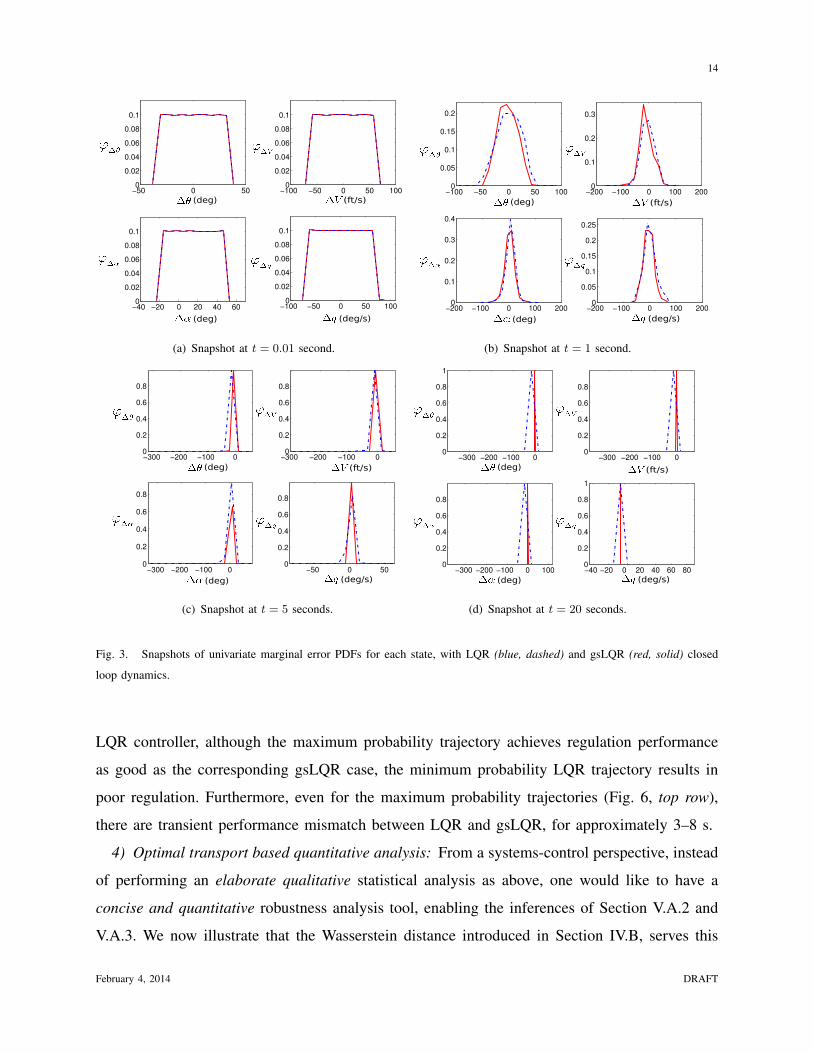
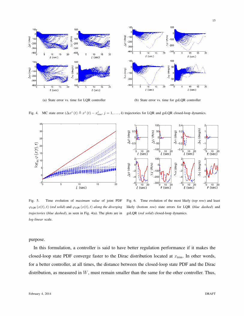
15
(a) State error vs time for LQR controller (b) State error vs time for gsLQR controller
Fig 4 MC state error (∆xj (t) xj (t)minus xjtrim j = 1 4) trajectories for LQR and gsLQR closed-loop dynamics
0 5 10 15 20minus5
0
5
10
15
20
25
30
35
(sec)
Fig 5 Time evolution of maximum value of joint PDF
ϕLQR (x(t) t) (red solid) and ϕLQR (x(t) t) along the diverging
trajectories (blue dashed) as seen in Fig 4(a) The plots are in
log-linear scale
0 10 20minus1
minus05
0
05
1
0 10 20minus100
minus50
0
50
100
0 10 20minus04
minus02
0
02
04
0 10 20minus2
minus1
0
1
2
0 10 20minus6
minus4
minus2
0
2
0 10 20minus300
minus200
minus100
0
100
0 10 20minus6
minus4
minus2
0
2
0 10 20minus2
minus1
0
1
2
(deg)
(fts)
(deg)
(degs)
(deg)
(fts)
(deg)
(degs)
(sec) (sec) (sec) (sec)
(sec) (sec) (sec) (sec)
Fig 6 Time evolution of the most likely (top row) and least
likely (bottom row) state errors for LQR (blue dashed) and
gsLQR (red solid) closed-loop dynamics
purpose
In this formulation a controller is said to have better regulation performance if it makes the
closed-loop state PDF converge faster to the Dirac distribution located at xtrim In other words
for a better controller at all times the distance between the closed-loop state PDF and the Dirac
distribution as measured in W must remain smaller than the same for the other controller Thus
February 4 2014 DRAFT
16
we compute the time-evolution of the two Wasserstein distances
WLQR (t) W (ϕLQR (x (t) t) ϕlowast (xtrim)) (12)
WgsLQR (t) W (ϕgsLQR (x (t) t) ϕlowast (xtrim)) (13)
The schematic of this computation is shown in Fig 7
Fig 7 Schematic of probabilistic robustness comparison for controllers based on Wasserstein metric The ldquodiamondrdquo denotes
the Wasserstein computation by solving the Monge-Kantorovich optimal transport The internal details of LQR and gsLQR
closed-loop dynamics blocks are as in Fig 1
Fig 8 indeed confirms the qualitative trends observed in the density based statistical analysis
mentioned before that LQR and gsLQR exhibit comparable immediate and asymptotic perfor-
mance Furthermore Fig 8 shows that for t = 3minus 8 seconds WLQR stays higher than WgsLQR
meaning the gsLQR joint PDF ϕgsLQR (x(t) t) is closer to ϕlowast (xtrim) compared to the LQR joint
PDF ϕLQR (x(t) t) This corroborates well with the transient mismatch observed in Fig 3(c)
As time progresses both WLQR and WgsLQR converge to zero meaning the convergence of both
LQR and gsLQR closed-loop joint state PDFs to the Dirac distribution at xtrim
Remark 1 At this point we highlight a subtle distinction between the two approaches of
probabilistic robustness analysis presented above (1) density based qualitative analysis and (2)
the optimal transport based quantitative analysis using Wasserstein distance For density based
qualitative analysis controller performance assessment was done using Fig 3 that compares
the asymptotic convergence of the univariate marginal state PDFs However this analysis is
only sufficient since convergence of marginals does not necessarily imply convergence of joints
Conversely the optimal transport based quantitative analysis is necessary and sufficient since Fig
February 4 2014 DRAFT
17
0 2 4 6 8 10 12 14 16 18 200
5
10
15
20
25
30
35
40
Wass
ers
tein
dis
tan
ce
(sec)
Fig 8 Comparison of time histories of W (ϕLQR(t) ϕlowast) (blue dashed star) and W (ϕgsLQR(t) ϕlowast) (red solid triangle)
8 compares the Wasserstein distance between the joint PDFs We refer the readers to Appendix
A for a precise statement and proof
Further since WLQR (t) rarr 0 for large t we can affirmatively say that the divergent LQR
trajectories are indeed of low-probability as hinted by Fig 5 and 6 Otherwise WLQR (t) would
show a steady-state error Thus the Wasserstein distance is shown to be an effective way of
comparing the robustness of controllers
B Robustness Against Parametric Uncertainty
1) Deterministic initial condition with stochastic parametric uncertainty Instead of the stochas-
tic initial condition uncertainties described in Section VA1 we now consider uncertainties in
three parameters mass of the aircraft (m) true x-position of cg (xcg) and pitch moment-of-
inertia (Jyy) The uncertainties in these geometric parameters can be attributed to the variable
rate of fuel consumption depending on the flight conditions For the simulation purpose we
assume that each of these three parameters has plusmn∆ uniform uncertainties about their nominal
values listed in Table I To verify the controller robustness we vary the parametric uncertainty
range by allowing ∆ = 05 25 5 75 and 15 As before we set the actuator disturbance w = 0
2) Simulation set up We let the initial condition be a deterministic vector x0 = xtrim +
xpert where xpert = [11803 rad 51058 fts 28370 rad 10minus4 rads]gt We keep the rest of the
February 4 2014 DRAFT
18
Fig 9 A schematic of how the support of a joint PDF evolves in the extended state space under parametric uncertainty For
ease of understanding we illustrate here a case for one state x and one parameter p Since x0 is deterministic but p is random
the initial joint PDF ϕ0 is simply the univariate parametric PDF ϕp(p) translated to x = x0 Consequently ϕ0 is supported on
a straight line segment (one dimensional subspace) in the two dimensional extended state space as shown in the left figure For
0 lt t lt infin due to state dynamics the samples (denoted as circles) on that line segment move in the horizontal (x) direction
while keeping the respective ordinate (p) value constant resulting the instantaneous support to be a curve (middle figure) If the
system achieves regulation then limtrarrinfin x(t) = xtrim forallp in the parametric uncertainty set resulting the asymptotic joint PDF
ϕinfin to be supported on a straight line segment (right figure) at x = xtrim
simulation set up same as in the previous case Notice that since p = 0 the characteristic
ODE for joint PDF evolution remains the same However the state trajectories along which the
characteristic ODE needs to be integrated now depend on the realizations of the random vector
p
3) Density based qualitative analysis Due to parametric uncertainties in p [m xcg Jyy]gt
we now have nx = 4 np = 3 and hence the joint PDF evolves over the extended state space
x(t) [x(t) p]gt isin R7 Since we assumed x0 to be deterministic both initial and asymptotic joint
PDFs ϕ0 and ϕinfin are degenerate distributions supported over the three dimensional parametric
subspace of the extended state space in R7 In other words ϕ0 = ϕp (p) δ (xminus x0) and ϕinfin =
ϕp (p) δ (xminus xtrim) ie the PDFs ϕ0 and ϕinfin differ only by a translation of magnitude x0 minus
xtrim 2= xpert 2 However for any intermediate time t isin (0infin) the joint PDF ϕ (x(t) t) has a
support obtained by nonlinear transformation of the initial support This is illustrated graphically
in Fig 9
The MC simulations in Fig 10 show that both LQR and gsLQR have similar asymptotic perfor-
mance however the transient overshoot for LQR is much larger than the same for gsLQR Hence
the transient performance for gsLQR seems to be more robust against parametric uncertainties
February 4 2014 DRAFT
19
(a) State error vs time for LQR controller (b) State error vs time for gsLQR controller
Fig 10 MC state error (∆xj (t) xj (t)minus xjtrim j = 1 4) trajectories for LQR and gsLQR closed-loop dynamics with
plusmn25 uniform uncertainties in p = [m xcg Jyy]gt ie p = pnominal (1plusmn∆) where ∆ = 25 and pnominal values are listed
in Table I
Similar trends were observed for other values of ∆
4) Optimal transport based quantitative analysis Here we solve the LP (10) with cost
cij = nnsumi=1
xi(t)minus xtrim 22 +nsumi=1
nsumj=1
np=3sumk=1
(pk (i)minus pk (j))2 (14)
with ςi being the joint PMF value at the ith sample location xi(t) = [xi(t) p(i)]gt and ςj being
the trim joint PMF value at the j th sample location [xtrim p(j)]gt Fig 11 and 12 show W (t)
vs t under parametric uncertainty for LQR and gsLQR respectively For both the controllers
the plots confirm that larger parametric uncertainty results in larger transport efforts at all times
causing higher value of W In both cases the deterministic (no uncertainty) W curves (dashed
lines in Fig 11 and 12) almost coincide with those of plusmn05 parametric uncertainties Notice
that in the deterministic case W is simply the Euclidian distance of the current state from trim
ie convergence in W reduces to the classical `2 convergence of a signal
It is interesting to compare the LQR and gsLQR performance against parametric uncertainty
for each fixed ∆ For 0 minus 3 s the rate-of-convergence for W (t) is faster for LQR implying
probabilistically faster regulation However the LQR W curves tend to flatten out after 3 s thus
slowing down its joint PDFrsquos rate-of-convergence to ϕinfin On the other hand gsLQR W curves
February 4 2014 DRAFT
20
0 5 10 15 200
1
2
3
4
5
6
time (s)
Was
sers
tein
Dis
tanc
e
052551015Deterministic
Parametric uncertainty
Fig 11 Time evolution of Wasserstein distance for LQR with
varying levels of ∆
0 5 10 15 200
1
2
3
4
5
6
time (s)
Was
sers
tein
Dis
tanc
e
052551015Deterministic
Parametric uncertainty
Fig 12 Time evolution of Wasserstein distance for gsLQR
with varying levels of ∆
exhibit somewhat opposite trend The initial regulation performance for gsLQR is slower than
that of LQR but gsLQR achieves better asymptotic performance by bringing the probability mass
closer to ϕinfin than the LQR case resulting smaller values of W Further one may notice that
for large (plusmn15) parametric uncertainties the W curve for LQR shows a mild bump around
3 s corresponding to the significant transient overshoot observed in Fig 10(a) This can be
contrasted with the corresponding W curve for gsLQR that does not show any prominent effect
of transient overshoot at that time The observation is consistent with the MC simulation results
in Fig 10(b) Thus we can conclude that gsLQR is more robust than LQR against parametric
uncertainties
C Robustness Against Actuator Disturbance
1) Stochastic initial condition uncertainty with actuator disturbance Here in addition to
the initial condition uncertainties described in Section VA1 we consider actuator disturbance
in elevator Our objective is to analyze how the additional disturbance in actuator affects the
regulation performance of the controllers
2) Simulation set up We let the initial condition uncertainties to be described as in Table
III and consequently the initial joint PDF is uniform Further we assume that the elevator is
February 4 2014 DRAFT
21
minus200
minus100
0
100
minus100
minus50
0
50
minus100
minus50
0
50
10minus4 10minus3 10minus2 10minus1 100 101 102 103 104minus100
minus50
0
50
(rads)
(dB)
(dB)
(dB)
(dB)
Fig 13 Singular values for the LQR closed-loop dynamics linearized about xtrim computed from the 4 times 1 transfer array
corresponding to the disturbance to states
subjected to a periodic disturbance of the form w(t) = 65 sin (Ωt) The simulation results of
Section VA1 corresponds to the special case when the forcing angular frequency Ω = 0 To
investigate how Ω gt 0 alters the system response we first perform frequency-domain analysis of
the LQR closed-loop system linearized about xtrim Fig 13 shows the variation in singular value
magnitude (in dB) with respect to frequency (rads) for the transfer array from disturbance w(t)
to states x(t) This frequency-response plot shows that the peak frequency is ω asymp 2 rads
3) Density based qualitative analysis To compare the LQR and gsLQR performance under
peak frequency excitation (as per linearized LQR analysis) we set Ω = ω = 2 rads and evolve
the initial uniform joint PDF over the LQR and gsLQR closed-loop state space Notice that the
LQR closed-loop dynamics is nonlinear and the extent to which the linear analysis would be
valid depends on the robustness of regulation performance Fig 14(a) shows the LQR state
error trajectories from the MC simulation It can be observed that after t = 10 s most of the
February 4 2014 DRAFT
22
(a) State error vs time for LQR controller (b) State error vs time for gsLQR controller
Fig 14 MC state error (∆xj (t) xj (t)minus xjtrim j = 1 4) trajectories for LQR and gsLQR closed-loop dynamics with
periodic disturbance w(t) = 65 sin (2t) in the elevator and initial condition uncertainties
LQR trajectories exhibit constant frequency oscillation with ω = 2 rads This trend is even
more prominent for the gsLQR trajectories in Fig 14(b) which seem to settle to the constant
frequency oscillation quicker than the LQR case
4) Optimal transport based quantitative analysis We now investigate the effect of elevator
disturbance w(t) = 65 sin (2t) and initial condition uncertainties via the optimal transport
framework In this case the computation of Wasserstein distance is of the form (11)
For the LQR closed-loop system Fig 15 compares the Wasserstein distances for no actuator
disturbance ie Ω = 0 rads (circles) actuator disturbances with Ω = 2 rads (solid line) and
Ω = 100 rads (dashed line) respectively It can be seen that the Wasserstein curves for Ω = 0
rads and Ω = 100 rads are indistinguishable meaning the LQR closed-loop nonlinear system
rejects high frequency elevator disturbance similar to the linearized closed-loop system as
observed in Fig 13 For Ω = 2 rads the Wasserstein curve reflects the effect of closed-loop
nonlinearity in joint PDF evolution till approximately t = 10 s For t gt 10 s we observe that the
LQR Wasserstein curve itself settles to an oscillation with ω = 2 rads This is due to the fact
that by t = 10 s the joint probability mass comes so close to xtrim that the linearization about
xtrim becomes a valid approximation of the closed-loop nonlinear dynamics This observation is
consistent with the MC simulations in Fig 14(a)
February 4 2014 DRAFT
23
For the gsLQR closed-loop system Fig 16 compares the Wasserstein distances with Ω =
0 2 100 rads It is interesting to observe that similar to the LQR case gsLQR closed loop
system rejects the high frequency elevator disturbance and hence the Wasserstein curves for
Ω = 0 rads and Ω = 100 rads look almost identical Further beyond t = 10 s the gsLQR
closed-loop response is similar to the LQR case and hence the respective Wasserstein curves
have similar trends However if we compare the LQR and gsLQR Wasserstein curves for Ω = 2
rads then we observe that gsLQR transient performance is slightly more robust than LQR
resulting lower values of Wasserstein distance for approximately 3 minus 5 seconds This transient
performance difference between LQR and gsLQR can also be seen in Fig 17 that shows the
time evolution of WLQR minusWgsLQR
VI CONCLUSION
We have introduced a probabilistic framework for controller robustness verification in the
presence of stochastic initial condition and parametric uncertainties The methodology is demon-
strated on F-16 aircraftrsquos closed-loop regulation performance with respect to two controllers
linear quadratic regulator (LQR) and gain-scheduled linear quadratic regulator (gsLQR) Com-
pared to the current state-of-the-art the distinguishing feature of the proposed method is that
Fig 15 Time evolution of Wasserstein distance for LQR with
elevator disturbance w(t) = 65 sin (Ωt)
Fig 16 Time evolution of Wasserstein distance for gsLQR
with elevator disturbance w(t) = 65 sin (Ωt)
February 4 2014 DRAFT
24
Fig 17 Time history of the difference between WLQR and WgsLQR with initial condition uncertainties and elevator disturbance
with Ω = 2 rads
the formulation is done at the ensemble level Hence the spatio-temporal evolution of the joint
PDF values are directly computed in exact arithmetic by solving the Liouville PDE via method-
of-characteristics Next robustness is measured as the optimal transport theoretic Wasserstein
distance between the instantaneous joint PDF and the Dirac PDF at xtrim corresponding to the
desired regulation performance Our numerical results based on optimal transport show that both
LQR and gsLQR achieve asymptotic regulation but the gsLQR has better transient performance
This holds for initial condition and parametric uncertainties with or without actuator disturbance
These conclusions conform with the Monte Carlo simulations
APPENDIX A
The purpose of this appendix is to prove that convergence of joint PDFs imply convergence
in respective univariate marginals but the converse is not true Here the convergence of PDFs
is measured in Wasserstein metric We first prove the following preparatory lemma that leads to
our main result in Theorem 1
Lemma 1 Let ϕi1 and ϕi2 be the respective ith univariate marginals for d-dimensional joint
PDFs ϕ1 and ϕ2 supported on Rx1 times Rx2 times times Rxd and Ry1 times Ry2 times times Ryd Let Wi
February 4 2014 DRAFT
25
W (ϕi1 ϕi2) i = 1 d and W W (ϕ1 ϕ2) then
dsumi=1
W 2i 6 W
2 (15)
Proof Notice that supp (ϕi1) = Rxi and supp (ϕi2) = Ryi forall i = 1 d For d-dimensional
vectors x = (x1 xd)gt y = (y1 yd)
gt by definition
W2
= infξisinM(ϕ1ϕ2)
intR2d
xminus y 22 ξ (x y) dx dy =
intR2d
xminus y 22 ξ (x y) dx dy (16)
where ξ (x y) is the optimal transport PDF supported on R2d Clearly
ϕi1 =
intR2dminus1
ξ (x y) dx1 dximinus1dxi+1 dxddy1 dyd (17)
ϕi2 =
intR2dminus1
ξ (x y) dx1 dxddy1 dyiminus1dyi+1 dyd (18)
Thus we have
W 2i = inf
ηisinM(ϕi1ϕ
i2)
intR2
(xi minus yi)2 η (xi yi) dxi dyi
=
intR2
(xi minus yi)2 η (xi yi) dxi dyi
6intR2
(xi minus yi)2 ξ (xi yi) dxi dyi (19)
where ξ (xi yi) is the (i i)th bivariate marginal of ξ (x y) Sincedsumi=1
(xi minus yi)2 = x minus y 22
the result follows from (19) after substituting
ξ (xi yi) =
intR2dminus2
ξ (x y) dx1 dximinus1dxi+1 dxd dy1dyiminus1dyi+1 dyd (20)
This completes the proof
Theorem 1 Convergence of Joint PDFs in Wasserstein metric implies convergence of uni-
variate marginals Converse is not true
Proof Using the notation of Lemma 1 when the joints ϕ1 and ϕ2 converge then W = 0
Hence from (15)dsumi=1
W 2i = 0 rArr Wi = 0 forall i = 1 d However Wi = 0 rArr W gt 0 Hence
the result
Remark 2 In our context of comparing LQR and gsLQR robustness (15) yields(nx=4sumj=1
W 2j
(ϕjLQR ϕ
jgsLQR
))12
6 W (ϕLQR ϕgsLQR) 6 W (ϕLQR ϕlowast) +W (ϕgsLQR ϕ
lowast) (21)
February 4 2014 DRAFT
26
where the last step is due to triangle inequality From Fig 8 we observe that with time both
W (ϕLQR ϕlowast) and W (ϕgsLQR ϕ
lowast) converge to zero As a consequence Wj
(ϕjLQR ϕ
jgsLQR
)= 0
(from (21)) j = 1 4 as evidenced by Fig 3
REFERENCES
[1] A Halder K Lee and R Bhattacharya ldquoProbabilistic Robustness Analysis of F-16 Controller Performance An Optimal
Transport Approachrdquo American Control Conference Washington DC 2013 Available at httppeopletamuedusimahalder
F16ACC2013Finalpdf
[2] BR Barmish ldquoProbabilistic Robustness A New Line of Researchrdquo UKACC International Conference on (Conf Publ
No 427) Controlrsquo96 Vol 1 pp 181ndash181 1996
[3] GC Calafiore and F Dabbene and R Tempo ldquoRandomized Algorithms for Probabilistic Robustness with Real and
Complex Structured Uncertaintyrdquo IEEE Transactions on Automatic Control Vol 45 No 12 pp 2218ndash2235 2000
[4] BT Polyak and R Tempo ldquoProbabilistic Robust Design with Linear Quadratic Regulatorsrdquo Systems amp Control Letters
Vol 43 No 5 pp 343ndash353 2001
[5] Q Wang and RF Stengel ldquoRobust Control of Nonlinear Systems with Parametric Uncertaintyrdquo Automatica Vol 38 No
9 pp 1591ndash1599 2002
[6] Y Fujisaki and F Dabbene and R Tempo ldquoProbabilistic Design of LPV Control Systemsrdquo Automatica Vol 39 No 8
pp 1323ndash1337 2003
[7] R Tempo and G Calafiore and F Dabbene Randomized Algorithms for Analysis and Control of Uncertain Systems
Springer Verlag 2005
[8] X Chen JL Aravena and K Zhou ldquoRisk Analysis in Robust ControlndashMaking the Case for Probabilistic Robust Controlrdquo
Proceedings of the 2005 American Control Conference pp 1533ndash1538 2005
[9] BR Barmish CM Lagoa and R Tempo ldquoRadially Truncated Uniform Distributions for Probabilistic Robustness of
Control Systemsrdquo Proceedings of the 1997 American Control Conference Vol 1 pp 853ndash857 1997
[10] CM Lagoa PS Shcherbakov and BR Barmish ldquoProbabilistic Enhancement of Classical Robustness Margins The
Unirectangularity Conceptrdquo Proceedings of the 36th IEEE Conference on Decision and Control Vol 5 pp 4874ndash4879
1997
[11] CM Lagoa ldquoProbabilistic Enhancement of Classical Robustness Margins A Class of Nonsymmetric Distributionsrdquo IEEE
Transactions on Automatic Control Vol 48 No 11 pp 1990ndash1994 2003
[12] P Khargonekar and A Tikku ldquoRandomized Algorithms for Robust Control Analysis and Synthesis Have Polynomial
Complexityrdquo Proceedings of the 35th IEEE Conference on Decision and Control Vol 3 pp 3470ndash3475 1996
[13] R Tempo EW Bai and F Dabbene ldquoProbabilistic Robustness Analysis Explicit Bounds for the Minimum Number of
Samplesrdquo Proceedings of the 35th IEEE Conference on Decision and Control Vol 3 pp 3470ndash3475 1996
[14] M Vidyasagar and VD Blondel ldquoProbabilistic Solutions to Some NP-hard Matrix Problemsrdquo Automatica Vol 37 No
9 pp 1397ndash1405 2001
[15] GC Calafiore F Dabbene and R Tempo ldquoResearch on Probabilistic Methods for Control System Designrdquo Automatica
Vol 47 No 7 pp 1279ndash1293 2011
[16] CM Lagoa and BR Barmish ldquoDistributionally Robust Monte Carlo Simulation A Tutorial Surveyrdquo Proceedings of the
IFAC World Congress pp 1ndash12 2002
February 4 2014 DRAFT
27
[17] Z Nagy and RD Braatz ldquoWorst-case and Distributional Robustness Analysis of Finite-time Control Trajectories for
Nonlinear Distributed Parameter Systemsrdquo IEEE Transactions on Control Systems Technology Vol 11 No 5 pp 694ndash
704 2003
[18] R E Bellman Dynamic Programming Princeton University Press 1957
[19] A Chakraborty P Seiler and GJ Balas ldquoNonlinear Region of Attraction Analysis for Flight Control Verification and
Validationrdquo Control Engineering Practice Vol 19 No 4 pp 335ndash345 2011
[20] P Seiler and GJ Balas and A Packard ldquoAssessment of Aircraft Flight Controllers using Nonlinear Robustness Analysis
Techniquesrdquo Optimization Based Clearance of Flight Control Laws Lecture Notes in Control and Information Sciences
Vol 416 Springer pp 369ndash397 2012
[21] A Chakraborty P Seiler and GJ Balas ldquoSusceptibility of FA-18 Flight Controllers to the Falling-Leaf Mode Linear
Analysisrdquo Journal of Guidance Control and Dynamics Vol 34 No 1 pp 57ndash72 2011
[22] A Halder and R Bhattacharya ldquoBeyond Monte Carlo A Computational Framework for Uncertainty Propagation in
Planetary Entry Descent and Landingrdquo AIAA Guidance Navigation and Control Conference Toronto Aug 2010
[23] A Halder and R Bhattacharya ldquoDispersion Analysis in Hypersonic Flight During Planetary Entry Using Stochastic
Liouville Equationrdquo Journal of Guidance Control and Dynamics Vol 34 No 2 pp 459ndash474 2011
[24] C Villani Topics in Optimal Transportation Vol 58 American Mathematical Society 2003
[25] C Villani Optimal Transport Old and New Vol 338 Springer 2008
[26] LT Nguyen ME Ogburn WP Gilbert KS Kibler PW Brown and PL Deal ldquoSimulator Study of StallPost-stall
Characteristics of A Fighter Airplane with Relaxed Longitudinal Static Stabilityrdquo NASA TP 1538 December 1979
[27] BL Stevens and FL Lewis Aircraft Control and Simulation John Wiley 1992
[28] R Bhattacharya GJ Balas A Kaya and A Packard ldquoNonlinear Receding Horizon Control of F-16 Aircraftrdquo Proceedings
of the 2001 American Control Conference Vol 1 pp 518ndash522 2001
[29] PE Gill W Murray and MA Saunders ldquoUserrsquos Guide for SNOPT Version 7 Software for Large-Scale Nonlinear
Programmingrdquo Technical Report Available at httpwwwccomucsdedusimpegpaperssndoc7pdf
[30] A Lasota and MC Mackey Chaos Fractals and Noise Stochastic Aspects of Dynamics Springer Vol 97 1994
[31] C Pantano and B Shotorban ldquoLeast-squares Dynamic Approximation Method for Evolution of Uncertainty in Initial
Conditions of Dynamical Systemsrdquo Physical Review E (Statistical Physics Plasmas Fluids and Related Interdisciplinary
Topics) Vol 76 No 6 pp 066705-1ndash066705-13 2007
[32] P Diaconis ldquoThe Markov Chain Monte Carlo Revolutionrdquo Bulletin of the American Mathematical Society Vol 46 No
2 pp 179ndash205 2009
[33] EF Camacho and C Bordons Model Predictive Control Vol 2 Springer London 2004
[34] A Halder and R Bhattacharya ldquoModel Validation A Probabilistic Formulationrdquo IEEE Conference on Decision and
Control Orlando Florida 2011
[35] A Halder and R Bhattacharya ldquoFurther Results on Probabilistic Model Validation in Wasserstein Metricrdquo IEEE
Conference on Decision and Control Maui 2012
[36] AS Mosek ldquoThe MOSEK Optimization Softwarerdquo Available at httpwwwmosekcom 2010
[37] H Niederreiter Random Number Generation and Quasi-Monte Carlo Methods CBMS-NSF Regional Conference Series
in Applied Mathematics SIAM 1992
February 4 2014 DRAFT
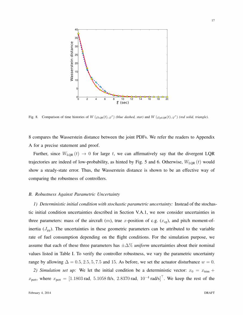
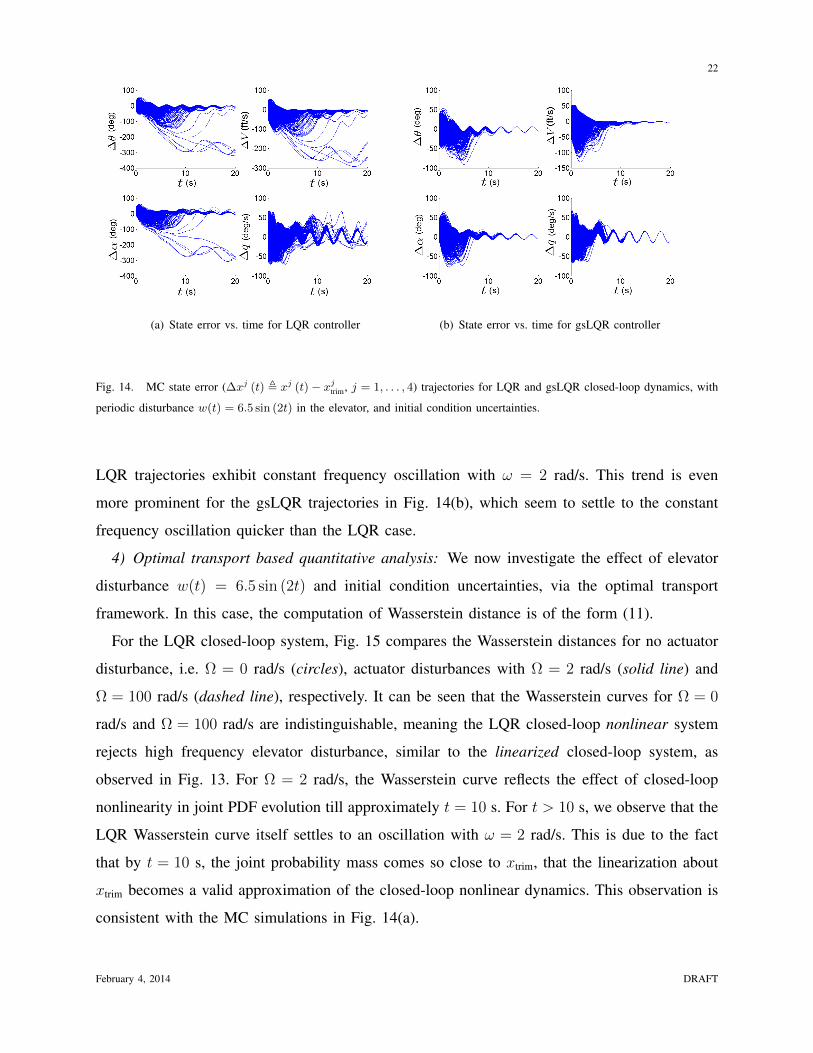
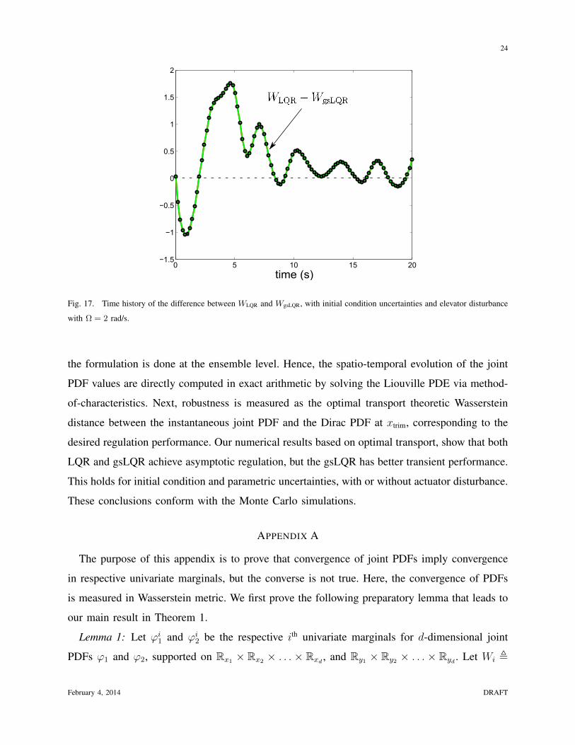
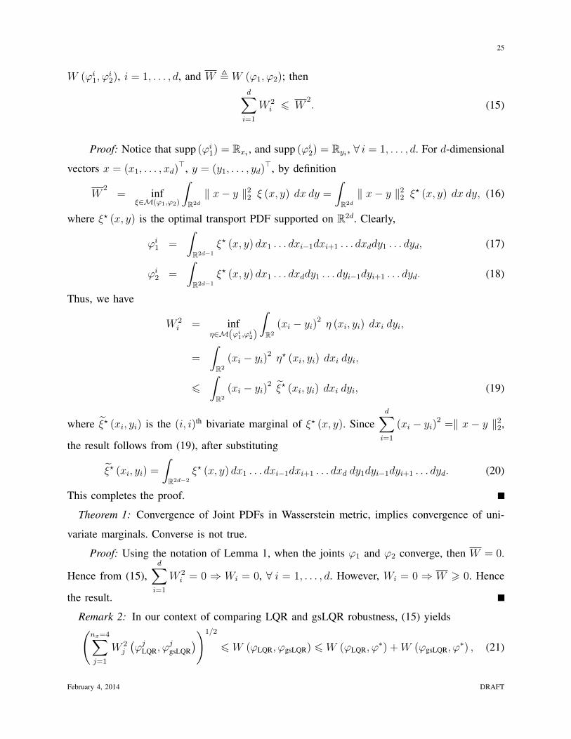