Optimal MOnetary Policy Rules when the Current Account Matters

This paper was written while Medina and Valdés were affiliated with the CentralBank of Chile. We thank P. García, L. O. Herrera, J. Marshall, K. Schmidt-Hebbel, R.Vergara, and participants in the Third Annual Conference of the Central Bank ofChile, “Monetary Policy: Rules and Transmission Mechanisms”, for helpful comments.All remaining errors are our responsibility. This paper presents the views of theauthors and does not necessarily represent in any way the positions or views of theMinistry of Finance, Chile.

65

OPTIMAL MONETARY POLICY RULES

WHEN THE CURRENT ACCOUNT MATTERS

Juan Pablo MedinaUniversity of California, Los Angeles

Rodrigo O. ValdésMinistry of Finance, Chile

Policymakers and the academic community have reached an in-creasing consensus during the last two decades: the primary objec-tive of monetary policy should be to control inflation (see, for example,King, 1999). A less settled issue is the appropriate role of the centralbank regarding other, secondary objectives. Some countries have ex-plicitly included unemployment (or the output gap) among the cen-tral bank’s objectives, whereas others make explicit reference to theoutput gap when explaining policy to the public. For example, theU.S. Federal Reserve has among its goals “to promote maximum em-ployment,” and the Reserve Bank of Australia has “the maintenanceof full employment” as an explicit objective in addition to price stabil-ity. The Sveriges Riksbank, the Bank of England, and even the Euro-pean Central Bank have identified output gap volatility as a reason tofollow a gradualist approach to controlling inflation. For example, theBank of England has stated that, in choosing among various alterna-tive paths to achieving the inflation target, the monetary authorityshould be concerned about deviations of the level of output from ca-pacity (see Svensson, 1999).

C

Monetary Policy: Rules and Transmission Mechanisms, edited by Norman Loayzaand Klaus Schmidt-Hebbel, Santiago, Chile. 2002 Central Bank of Chile.

66 Juan Pablo Medina and Rodrigo O. Valdés

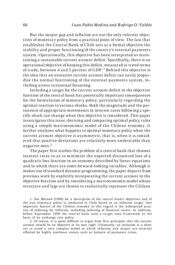
But the output gap and inflation are not the only relevant objec-tives of monetary policy from a practical point of view. The law thatestablishes the Central Bank of Chile sets as a formal objective thestability and proper functioning of the country’s external paymentssystem. Operationally, this objective has been interpreted as main-taining a sustainable current account deficit. Specifically, there is anoperational objective of keeping this deficit, measured at trend termsof trade, between 4 and 5 percent of GDP.1 Behind this objective isthe idea that an excessive current account deficit can easily jeopar-dize the normal functioning of the external payments system, in-cluding access to external financing.

Including a target for the current account deficit in the objectivefunction of the central bank has potentially important consequencesfor the formulation of monetary policy, particularly regarding theoptimal reaction to various shocks. Both the magnitude and the per-sistence of appropriate movements in interest rates following a spe-cific shock can change when this objective is considered. This paperinvestigates this issue, deriving and comparing optimal policy rulesusing a simple macroeconomic model of the Chilean economy. Itfurther analyzes what happens to optimal monetary policy when thecurrent account objective is asymmetric, that is, when it is consid-ered that positive deviations are relatively more undesirable thannegative ones.2

The paper first studies the problem of a central bank that choosesinterest rates so as to minimize the expected discounted loss of aquadratic loss function in an economy described by linear equationsand in which there are some forward-looking variables. Although itmakes use of standard dynamic programming, the paper departs fromprevious work by explicitly incorporating the current account in theobjective function and by considering a macroeconomic model whosestructure and lags are chosen to realistically represent the Chilean

1. See Massad (1998) for a description of the central bank’s objectives and ofthe way monetary policy is conducted in Chile based on an inflation target. Oneimportant feature of the Chilean economy in this regard is the widespread prac-tice of indexing for inflation, including indexing of financial assets. In addition,before September 1999 the central bank used a target zone framework as thebasis of its exchange rate policy.

2. Of course, it is quite difficult to argue from first principles that the currentaccount should be an objective in its own right. Ultimately, its inclusion is a shortcut to avoid a very complex model in which inflation and output are severelyaffected by highly nonlinear events such as balance of payments crises.

Optimal Rules when the Current Account Matters 67

economy.3 The model structure is similar to that of a simple centralbank macroeconomic projection model. It includes equations for theoutput gap, the absorption-output gap, a Phillips curve, uncoveredinterest rate parity, and a term structure. Using this model, we in-vestigate how optimal policy reactions change when the current ac-count matters, and the implications of incorporating the output gapamong the central bank’s objectives.

The paper then studies the consequences of having an asymmet-ric objective for the current account. This is done within a consider-ably simpler framework, as otherwise it would be difficult to solvethe central bank’s problem. The economy is described by a centralbank loss function that depends on inflation and the absorption-out-put gap, with two linear equations describing their evolution. Again,the central bank has to choose interest rates so as to minimize theexpected discounted loss, this time of a nonquadratic loss function.The solution method we use in this case is based on standard dy-namic programming using a convenient discretization of the economy.We investigate how optimal policy reactions change both with theasymmetry in objectives and with uncertainty about future shocks.4

It is important to clarify at the outset that by an optimal reactionwe mean the best possible policy rule in terms of maximizing theobjective function in the context of the model under analysis. It is notnecessarily the best policy for day-to-day policymaking, because, bydefinition, any model is an incomplete description of reality. Actualpolicymaking might take into account these rules—indeed, they arequite appealing as they give precise answers to a quite complex prob-lem of combined lagged effects. However, policymakers should alsoevaluate the implications of developments that are not considered inthe model. In other words, the optimality of the rules we study ismodel-specific.

The main results of the paper yield relevant policy conclusions.For example, we find that including the current account among theobjectives of the central bank has important consequences for opti-mal policy reactions. Interest rates react vigorously (and without muchpersistence) to shocks that affect the current account deficit, but are

3. Svensson (2000), Ryan and Thompson (1999), and many others study opti-mal policy rules in inflation targeting frameworks for open economies. Amongother issues, these papers analyze the usefulness of monetary conditions indexesand the merits of targeting inflation of nontraded goods.

4. Because with asymmetric objectives the problem is not linear-quadratic,there is no certainty equivalence.


less responsive to output gap and inflation shocks when the currentaccount is among the objectives. If the current account does not mat-ter, optimal policy rules change considerably when the central bankcares about the output gap. However, these changes are far less dra-matic if the central bank already has the current account among itsobjectives. An asymmetric current account objective does not greatlychange the optimal reactions to demand shocks, but it makes mon-etary policy clearly more aggressive toward positive inflation shocks.The change in this policy reaction is economically relevant. Finally,when there is an asymmetric current account objective, a higher vola-tility in current account shocks generates a more aggressive mon-etary policy.

The paper is organized as follows. Section 1 describes the struc-ture of the economy as modeled, as well as monetary policy objec-tives in a standard linear-quadratic framework. Section 2 presentsthe method for solving the central bank’s problem and compares op-timal policy rules for alternative central bank preference parametersusing a realistic model estimate. Section 3 studies policy rules in asimpler economy but one in which current account objectives areasymmetric. Finally, section 4 presents some concluding remarks.

1. THE ECONOMY

The economy is described by a series of state variables, some ofwhich are exogenous, while others are endogenous, predetermined,and subject to stochastic shocks, and the rest are endogenous andforward-looking. These variables evolve according to a simple linearmacroeconomic model in which monetary policy affects some vari-ables instantaneously and others with a lag.5 The exogenous vari-ables represent the fundamentals for the economy and follow simplestochastic processes. The economy is endowed with a central bank,which has an explicit objective function. The frequency of the empiri-cal counterpart of the model is quarterly, and we assume that vari-ables are observed contemporaneously.6

5. The model we consider is not immune to the Lucas critique, althoughexpectations are completely rational and the public knows the central bank’sobjectives. However, the Lucas critique is not that relevant when policy shocksare small (which is the case considered in this paper).

6. One way of interpreting this assumption is to consider that monetary policychooses end-of-period interest rates. An alternative is to consider that actual (off-model observed) short-term projections are very good (within a quarter).


All variables in the model are measured as deviations from their(possibly stochastic) long-run trend and consequently are stationary.For example, rt represents deviations of the interest rate with re-spect to its long-run trend.7

1.1 Monetary Policy Objectives

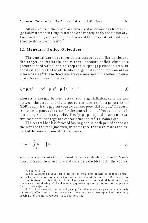
The central bank has three objectives: to keep inflation close tothe target, to maintain the current account deficit close to apreannounced value, and to keep the output gap close to zero. Inaddition, the central bank dislikes large and sudden movements ininterest rates.8 These objectives are summarized in the following qua-dratic loss function of period t:

( ) ,21

222−π −µ+µ+µ+πµ= ttrtytcctt rryccl

where πt is the gap between actual and target inflation, cct is the gapbetween the actual and the target current account (as a proportion ofGDP), and yt is the gap between actual and potential output.9 The term(rt

_ rt-1)2 captures the costs for the central bank of frequent and sud-den changes in monetary policy. Lastly, µπ, µcc, µy, and µr are nonnega-tive constants that together characterize the central bank type.

The central bank is forward looking and in each period t choosesthe level of the real (indexed) interest rate that minimizes the ex-pected discounted sum of future losses:

,E0

Ωδ= ∑

∞

=ττ+

τttt lL

where Ωt represents the information set available in period t. More-over, because there are forward-looking variables, both the central

7. See note 13.8. See Woodford (1999a) for a derivation from first principles of these prefer-

ences for smooth movements in the policy instrument. Massad (1998) makes thecase for instrument stability in Chile. The concern of the central bank regardingthe normal functioning of the domestic payments system gives another argumentfor such an objective.

9. In this framework the authority recognizes that monetary policy can have onlytemporary effects on output. Moreover, there are no intertemporal inconsistencyproblems of the Barro-Gordon type. See note 13.

(2)

(1)


bank and the public know that the former can reoptimize in eachperiod. Hence, the only possible solution is a discretionary one.10

Therefore, the optimal policy rule has the form rt = FXt, where Xtis the vector of predetermined variables and F is a vector of con-stants to be endogenously determined (see Backus and Driffill,1986, and Söderlind, 1999a, for further details).

1.2 State Variables

There are three fundamental exogenous variables in thiseconomy: the terms of trade (in logarithms) (tot), the country riskpremium (ϕ), and the international real interest rate (r

t * ) . We

assume that these three variables are stationary (or that they aretransformed so as to eliminate any trend). Their law of motion isgiven by the following equations:

,11tottttotttott rtottot ξ+ρ+ρ= ∗

−− (3)

,1rttrt rr ξ+ρ= ∗

−∗ and (4)

,1ϕ

−ϕ ξ+ϕρ=ϕ ttt (5)

respectively, where 0 < ρj < 1 and ξ jt are i.i.d. shocks (j = tot, r*,and ϕ).11

Domestic inflation moves according to inflation in traded goodsand in nontraded goods. Traded goods inflation, in turn, depends oninternational prices and the exchange rate, and nontraded goodsinflation depends (because of indexation) on previous inflation, oninflation expectations in previous periods, and on the output gap

10. A solution involving a commitment would attain a better outcome (seeWoodford, 1999b). However, like Svensson (1999), we assume that a commitmenttechnology is not available. Thus, the only realistic solution is discretionary.

11. A more realistic approach would be to model the risk premium as anendogenous variable that depends on domestic variables such as the current ac-count. Then an increase in the current account deficit would cause a nominaldevaluation following a rise in the risk premium. However, considering this pos-sibility would only add an additional, indirect concern of the central bank regard-ing the current account, without substantially changing the main results.

r


(according to a standard accelerationist Phillips curve). In particu-lar, the (annualized) inflation gap evolves according to

( ) ,1 π−ωπ+πω−=π Nt

Ttt (6)

where π Tt is tradables inflation, π Nt is nontradables inflation, π is the

inflation target, and ω is a constant parameter. Tradables inflation isdetermined as follows:

( )( ) ,ˆL 11TtttT

Tt e ξ+π+α=π ∗

−− (7)

where α'(L) is a polynomial in the lag operator L, et is the nominaldevaluation, π *t is international inflation, and ξ Tt is an i.i.d. shock.This specification assumes that the weak version of purchasing powerparity obtains for tradables (controlling for changes in value-addedtaxation and tariffs) and that there is no instantaneous pass-through.On the other hand, nontradables inflation evolves according to

( ) ( )[ ] ( ) ,L'|FEL' 111LNttyttFt

Nt y ξ+α+Ωπα+πα=π −+π−π (8)

where α'πF (F) is a polynomial in the forward (lead) operator. This

means that ( )11 |E −+ Ωπ tt is a predetermined variable in period t.12

Let us define the real exchange rate (RER) as tttt ppeq ∗=and assume, without loss of generality, that . Then the inflationgap equation can be written as

( ) ( ) ( )[ ]( ) ,L

|FELˆL 111L1

π

−+π−π−

ξ+α+

Ωπα+πα+α=π

tty

ttFttTt

y

q(9)

where αT (L) = (1 _ ω)α'T(L), απL(L) = ωα'

πL(L) + (1 _ ω)α'T(L), απF (F)

= ωα'πF(F), αy(L) = ωα'

y(L) and ( ) Tt

Ntt ξω−+ωξ=ξπ 1 . Furthermore,

^

12. This structure is based on one of the projection models used at the CentralBank of Chile and is similar to the price equation derived from first principles inSvensson (2000).

0=π

'

'


in order to preserve homogeneity in prices we assume that( ) ( )[ ] ( ) ( ) 11'11'1' =αω−+α+αω ππ TFL . Notice that in this frame-

work monetary policy affects inflation through three different chan-nels: the output gap, the exchange rate, and lagged expectations offuture monetary policy (and hence future inflation).

The RER is a forward-looking variable that is determined by theuncovered interest parity condition:

( ) ( ) .25.0E 1 tttttt rrqq ϕ+−+Ω= ∗+ (10)

Besides the short-term real interest rate controlled by the centralbank, there is a long-term interest rate determined as a forward-looking variable in the bond market. According to the expectationhypothesis of the term structure, the behavior of the long-term inter-est rate Rt can be approximated by

( ) ( ) ,E1 1 tttt RrR Ωλ−+λ= + (11)

where λ is a constant that negatively depends on the bond duration.The output gap has some persistence and reacts with lags to the

interest rates, the terms of trade, and the RER:

( ) ( ) ( ) ( )( ) ,L

LLLL

1

1111

yttq

ttottrtRtyt

q

totrRyy

ξ+β+

β+β+β+β=

−

−−−−

(12)

where ξ yt is an i.i.d. shock. This equation represents a standarddynamic IS curve.

To construct the ratio of the current account (proxied by the tradebalance) to GDP, we consider a linear approximation that depends onthe gap between absorption and output (denoted by y dt ), the terms oftrade, the output gap, and the RER. A first-order (log) Taylor expan-sion of the trade balance yields the following approximation:

,100 tttdtt totkykqkycc ++−−= (13)

where k0 is the ratio of the trade balance to GDP during the expan-sion year (2 percent in 1997), and k1 is the ratio of exports to GDP


during that year (30 percent in 1997). The current account deficitduring the expansion year was 4.8 percent of GDP.

Finally, we assume that the absorption-output gap has some per-sistence and depends on interest rates, the terms of trade, and theRER. In particular, this gap is determined by the following equation:

( ) ( ) ( ) ( )( ) ,L

LLLL

1

1111

dttq

ttottrtRdtd

dt

q

totrRyy

ξ+γ+

γ+γ+γ+γ=

−

−−−−(14)

where dtξ is an i.i.d. shock. In order to be consistent with our prior

definition of yt, we consider dty as the gap between, on one hand, the

difference between actual and trend absorption and, on the other, theoutput gap.13 Of course, because both equations include output in theleft-hand side, and both represent cyclical movements of the economy,equations (14) and (12) are closely related. Thus the shocks y

tξ and dtξ

need not be orthogonal. In the exercises below we consider both inde-pendent and common shocks to both equations.

In sum, the economy is described by equations (3) to (5) and (9) to(14). Appendix A presents the estimation and calibration results ofthese equations using Chilean quarterly data. We choose a lag struc-ture in each equation so as to maximize the realism and fit of themodel, even though this strategy generates several state variables.

2. SOLUTION

The solution of the model requires us to rewrite the model so asto represent it in the state-space form. Once it is represented in thisway, one can apply directly the algorithms described in Backus andDrifill (1986), Svensson (1994), and Söderlind (1999b). As mentionedbefore, we consider a discretionary solution.

2.1 State-Space Representation

Following the same notation as Svensson (2000), let Xt be the (col-umn) vector of predetermined variables, Yt the (column) vector of

13. In this framework, therefore, we study the effects of monetary policy onthe current account without considering secular trends in the expenditure-outputgap. This is consistent with the idea that the central bank is only capable of choosing(temporary) deviations of the real interest rate with respect to its long-run trend.The latter is actually endogenous and responds to the aforementioned secular trend.


variables that enter as arguments in the central bank’s loss function,xt the (column) vector of forward-looking variables, and ξt the (col-umn) vector of shocks. Considering the lag structure embedded inthe model estimation presented in appendix A, one has

,'

,,

,,,,,,,,,,,,,,X

11

132132121

ππππϕ=

−−

−−−−−−−∗

−−

dttt

ttttttttttttttt

yRr

yyqqqrtottottot

( ) ,' ,,,Y 1−−π= tttttt rrycc

( ) ( )[ ] ,'

E,E,,x 1211 −+−+ ΩπΩπ= ttttttt qR

( ) .'

,0,0,0,,0,0,0,,0,0,0,,,0,0, dt

yttt

rt

tottt ξξξξξξ= πϕ?

Let n1, n2, n3, and n = n1+ n2 be the dimensions of Xt, xt, Yt, and Zt,respectively. In the particular model we consider, n1 = 17, n2 = 4, andn3 = 4. Let Zt = (X '

t, x 't) be the vector that describes the state of

the economy. Using these definitions, the model can be written inthe following way (in the state-space):

( ) ,0

BrAZxE

X

1

1

++=

+

+

+ 1

t

tttt

t ?O

,rCZCY trtzt +=

,KYYl 'ttt =

where A is a n × n matrix, B is a n × 1 column vector, Cz is an3 × n matrix, Cr is a n3 × 1 column vector, and K is a n3 × n3 diagonalmatrix with (µπ, µcc, µy, µr) in the diagonal. Appendix B describes theconstruction of these matrices in detail.

The solution to the central bank’s problem is characterized by apolicy function of the following form:

and

(15)

(16)

(17)'


rt = FXt , (18)

where F is a 1 × n1 row vector to be endogenously determined.The solution also characterizes the evolution of the forward-look-

ing variables according to the following linear function:

,HXx tt = (19)

where H is a n2 × n1 matrix to be endogenously determined.Hence the dynamics of the economy are given by equations (18)

and (19) and the following pair of equations:

,XMX 1111 ++ += ttt ? and (20)

( ) ,XFCHCCY 21 trzzt ++= (21)

where M11, Cz1, Cz2 are n1 × n1, n3 × n1 and n3 × n2 matrices, respec-tively, corresponding to the partitions of

,MMMM

0F

BAM2221

1211

=

+≡ and

[ ] ,CCC 21 zzz =

according to Xt and xt.In order to find the matrices F and H we use the algorithm

mentioned above.

2.2 Optimal Reaction Functions

The optimal policy rule depends both on the structure of theeconomy and on the preferences of the central bank. These prefer-ences, in turn, are described by a discount rate and by a set of rela-tive weights for the loss function in equation (1). We consider adiscount factor of 0.99 and four sets of weights for equation (1) andthus define four types of central banks. The “hawk” type (H) has in-flation as its almost unique objective; the “dove” type (D) has as its


objectives both inflation and the output gap; the objectives of the“strict condor” type (SC) are inflation and the current account deficit;and those of the “flexible condor” type (FC) include inflation, the cur-rent account deficit, and the output gap. We assume that all fourcentral bank types dislike large changes in interest rates and there-fore have µr > 0. Table 1 presents the weights (µs) of the loss functionfor each of these central bank types.14

Table 2 presents the optimal reaction functions for each of thefour types. Each column corresponds to the vector F ' , which, multi-plied by the vector Xt, yields the optimal interest rate deviation forperiod (quarter) t. For example, if the central bank is of the hawktype, it will increase the (indexed) interest rate by 0.45 percentagepoint after a 1-percentage-point upward shock to inflation.15

Examining the dynamic reaction of the interest rate to alterna-tive shocks is another way of analyzing optimal policy rules. Thesereactions show the path of interest rates that would prevail if therule is followed and no other shocks occur, and thereby include reac-tions to expected future movements in other endogenous variables.

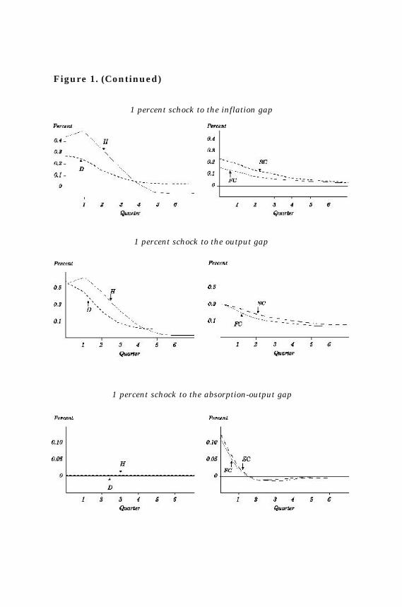
Figure 1 presents the path of interest rates between quarter 0 (onimpact) and quarter 7 following different exogenous shocks. Besidesthe six basic (structural) shocks of the model, we consider a combinedshock to output and the absorption-output gap, which can be thoughtof as the case of an overheated economy. The figure presents the reac-tions of the four central bank types to such a shock. The panels on theleft show the reactions of central bank types H and P, whereas those onthe right ones show the reactions of types SC and FC.

14. The central bank preferences are “deep” parameters unaffected by thestructure of the economy (for example, the degree of indexation). The structureof the economy modifies the optimal reaction functions, not preferences.

15. Notice that the interest rate persistence depends on both the parameterfor rt-1 and that for Rt-1.

Table 1. Preference Parameters for the Four CentralBank Types

Type of central bank µ π µ cc µy µr

Hawk 0.95 0.00 0.05 0.10Dove 0.50 0.00 0.50 0.10Strict condor 0.65 0.30 0.05 0.10Flexible condor 0.35 0.30 0.35 0.10

Source: Authors’ definitions.


The results of table 2 and figure 1 have implications in at leastthree dimensions (besides the numerical results, which may be use-ful as a benchmark for policymaking). First, once the current ac-count is part of the central bank’s objectives, optimal policy reactionschange in many respects, sometimes substantially. As expected, theSC and FC types respond to shocks to the absorption-output gap andto the terms of trade in a very different way than do types H and D.These two shocks have direct effects on the current account, for whichthe latter two central banks do not care. Interestingly, types SC andFC are less responsive to shocks to the international interest rateand the risk premium than types H and D, respectively. More impor-tant, when there is a target for the current account, monetary policyis clearly less aggressive in responding to shocks to inflation (com-pare type H with type SC) and to the output gap. All these differencesare economically relevant.

Table 2. Optimal Policy Functions by Central Bank Type

Central bank type

Strict FlexibleVariable Hawk Dove condor condor

tot t –0.02 –0.01 –0.11 –0.10

tot t -1 0.02 0.03 0.05 0.05

tot t -2 0.01 0.02 0.01 0.01

r*t 0.87 0.43 0.52 0.34

ϕ t 0.72 0.32 0.43 0.27

q t -1 –0.13 –0.06 –0.09 –0.06

q t -2 –0.09 –0.04 –0.07 –0.04

q t -3 –0.11 –0.05 –0.06 –0.04

πt 0.45 0.28 0.24 0.17

π t -1 0.32 0.19 0.17 0.11

π t -2 0.19 0.11 0.10 0.07

π t -3 0.09 0.05 0.04 0.03

y t 0.57 0.60 0.31 0.33

y t -1 0.12 0.07 0.06 0.04

r t -1 0.28 0.12 –0.04 –0.07

R t -1 –0.27 –0.37 –0.15 –0.20

y dt 0.00 0.00 0.13 0.12

Source: Authors’ calculations.

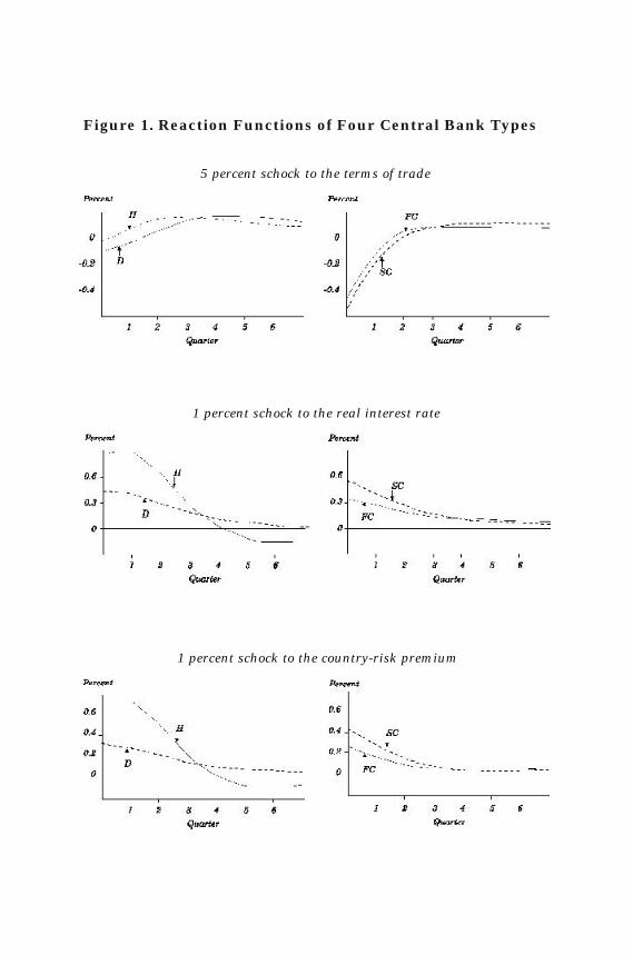
Figure 1. Reaction Functions of Four Central Bank Types

5 percent schock to the terms of trade

1 percent schock to the real interest rate

1 percent schock to the country-risk premium

1 percent schock to the inflation gap

1 percent schock to the output gap

1 percent schock to the absorption-output gap

Figure 1. (Continued)


Second, the results show that, in general, reactions are less per-sistent for shocks that directly and indirectly affect the current ac-count when the current account matters. This is probably due tothe relatively lower persistence in the absorption-output gap in com-parison to other variables. However, the reaction to inflation andoutput shocks is more persistent in types SC and FC than in typesH and D.

Finally, the differences in optimal rules that arise when the cen-tral bank incorporates the output gap among its objectives are farless dramatic when the current account is already one of its objec-tives. Indeed, the differences between the reactions of types H andD are considerably more important than the differences betweenthose of types SC and FC. One case in which this difference appearsmost clearly is in the dynamic central bank reaction to an inflationshock—probably the key issue in monetary policymaking. In thiscase type SC is only marginally more hawkish than type FC. Thusone can conclude that incorporating the output gap into the centralbank’s objectives does not appear to be crucial when the currentaccount already matters. The intuition for this result is simple: thecurrent account also presents a trade-off for monetary policy, be-cause a more aggressive response to an inflation shock generates alarger current account deviation. However, for this result to hold, itis necessary to have a symmetric current account objective. Thenext section analyzes optimal policy reactions when this objective isasymmetric.

Simultaneous 1 percent schock to the output gap and the absorption-output gap

Figure 1. (Continued)



3. OPTIMAL MONETARY POLICY WITH AN ASYMMETRIC

CURRENT ACCOUNT OBJECTIVE

Ultimately, behind the objective of keeping the current accountunder control is the notion that an “excessive” deficit usually bringsabout a serious balance of payments crisis, in which voluntary financ-ing disappears and the economy enters a deep recession. The con-verse, however, is not true: too small a deficit is not considered to bea threat to external stability. But the loss function described by equa-tion (1) is symmetric, treating positive and negative deviations asequally undesirable. Therefore the rules we have derived are, by con-struction, symmetric. This section investigates the implications formonetary policy of having an asymmetric loss function for the cur-rent account.

We analyze two issues that arise with asymmetric objectives.First, we investigate how much optimal reactions change, in responseto both price and demand (current account) shocks. Second, we ana-lyze whether optimal monetary policy changes when the volatility ofshocks increases. We evaluate both how policy changes and the eco-nomic relevance of these changes.

Departing from the linear-quadratic framework (that is, from asymmetric current account objective) has the benefit of allowing for amore realistic loss function, but at the same time, it seriously compli-cates the problem. In the linear-quadratic problem we were able tofind closed-form solutions of the form rt = FXt, whereas in this casewe have to resort to numerical simulations. To be able to solve thecentral bank’s problem, we have to simplify the model of the economysubstantially. In particular, we calibrate a simple stochastic, two-equa-tion, backward-looking economy with two state variables, namely,inflation and the absorption-output gap, and directly associate thelatter with the current account deficit. For simplicity, we assumethat a positive absorption-output gap has inflationary consequences.16

Moreover, we do not consider any preferences over interest rate vari-ability, nor do we consider bounds for possible interest rate values.Thus the rules we derive will in general prescribe a more aggressive

16. It should be stressed that this is a simplification. There is no reason for thisgap to have direct inflationary consequences. What happens is that this gap isusually highly correlated with the output gap, which does affect inflation.


monetary policy than what a central bank would normally follow.Accordingly, rather than taking the quantitative results we derive atface value, they should be analyzed relative to the baseline scenarioof rules for a symmetric current account objective (derived from astandard quadratic loss function).

3.1 A Simpler Economy

The economy is described by the following two equations:

,11π

−− ε+α+π=π tdtytt y and (22)

,11yttr

dty

dt ryy ε+β+β= −− (23)

where, as before, πt is the inflation gap in period t, dty is the absorp-

tion-output gap, rt is the real (or indexed) interest rate (again mea-sured as a deviation from its long-run trend), and πεt and y

tε areserially uncorrelated mean-zero stochastic shocks. The quantities αy,βr, and βy are constant parameters.

As before, the central bank’s problem at time t is to choose asequence of interest rates ∞

=τ+ 0ttr so as to minimize the intertem-poral loss function in equation (2). Let x t be the vector with the statevariables, . We seek to characterize the interest rate se-quence through a time-invariant (and probably nonlinear) policy func-tion for a loss function of the following type:

( ) ( ) ( )( ) ( )

∞∈+π

∞∈+π=

, 0,for ba

0,-for ba22

22

dt

dtHt

dt

dtLt

tyy

yyxl (24)

where a, bL, and bH are positive constants. The asymmetric currentaccount objective is described by bL < bH.

Therefore the central bank’s problem is to set interest rates in orderto minimize equation (2) with equation (24) subject to equations (22) and(23). We consider three alternative central bank types: quadratic, asym-metric, and one-sided. Table 3 presents the preference parametersof each. The quadratic central bank has the standard symmetric loss

( )'x dttt y,p=


function, the asymmetric central bank cares considerably more aboutpositive deviations of the current account from its target than aboutnegative ones, and the one-sided central bank dislikes positive cur-rent account deviations (and inflation) only. In all cases, on average,there is a 2:1 weight relation between inflation and current accountgap deviations.

We calibrate the model using the following parameter values:αy = 0.5, βy = 0.6, βr = _0.5, S.D.( πεt ) = 0.8 percent, S.D.( y

tε ) = 0.8percent, and zero covariance between shocks (where S.D. representsthe standard deviation). These parameters are approximately in linewith the estimation of equations (22) and (23) with Chilean data, withthe caveat that we use the output gap in the former equation (seenote 16).17 The frequency of the real-world counterpart of the modelcan be thought of as being either quarterly or semiannual.

3.2 Solution

To solve the problem we discretize the economy along the linesfollowed by Medina and Valdés (2002) and apply standard dynamicprogramming techniques. It should be mentioned that this approxi-mation yields quite accurate solutions for the linear-quadratic case.

Figure 2 shows the optimal policy functions for the central bank’sproblem under alternative combinations of inflation and the absorp-tion-output gap. In each panel the x-axis shows a gap deviation, andthe y-axis shows the optimal policy reaction (given by the interestrate deviation) of each of the central bank types.

Table 3. Loss Functions of Alternative Central Bank Types

Central bank type

Variable Quadratic Asymmetric One-sided

a 1.00 1.00 1.00bL 0.50 0.20 0.00bH 0.50 0.80 1.00δ 0.95 0.95 0.95

17. The estimation of equation (22) yields a considerably higher inflationvolatility. However, as shown by Magendzo (1998), in Chile there is close relationbetween the level and the volatility of inflation. The estimation of the same equa-tion using the difference between actual and long-run trend inflation yields astandard deviation of 0.2 percent.

Source: Authors’ definitions.

Figure 2. Optimal Policy Functions with an AsymmetricCurrent Account Objective


Reaction to inflationAbsorption-output gap = 0

Reaction to absorption-output gapinflation gap = 0

Reaction to inflation gapabsorption-output gap = 1


Reaction to inflationabsorption-output gap = _1

Reaction to absorption-output gapinflation gap = _1


The results show two interesting features. First, and more im-portant, the asymmetric current account objective generates a moreaggressive response to positive inflation shocks. The intuition for thisis straightforward: there is no trade-off involved. The differences arequite large. For example, if the current account gap is zero while theinflation gap is 3 percent, a one-sided central bank will increase in-terest rates by almost twice as much as the symmetric one, and anasymmetric central bank will increase them by one-third more thanthe symmetric one. In the case of negative inflation shocks, the asym-metry generates a less aggressive monetary policy (higher interestrates). Hence the two effects together imply that a central bank withan asymmetric current account objective can end up having inflation,on average, below its target.18

Second, at least for the case in which there is a negative or a zeroinflation gap, the asymmetric current account objective does not greatlyaffect the optimal policy response to demand (current account) shocks.The reason for this result is that even if an expenditure gap does notmatter directly, it can matter indirectly through its future impact oninflation, especially when inflation has a unit root. This is not the caseif there is a positive absorption-output gap and a positive inflation gap.In this case monetary policy is more aggressive because the no-trade-off argument applies.

Figure 3 illustrates what happens to optimal policy reactionswhen the standard deviation of current account shocks increases.As one might expect, when the standard deviation rises from 0.8percent (the baseline case) to 1.4 percent, the reactions of thecentral bank are more aggressive against inflation. However, thesechanges are not of great economic relevance. Only when the stan-dard deviation rises to 2 percent do the differences start to be-come important, although they still are less important than thedifferences created by the asymmetry itself. In the case of nega-tive inflation shocks, we find that a higher volatility of shocks alsomakes monetary policy more aggressive. One possible explanationis that when the inflation gap is very negative, a higher demandvolatility risks a movement toward an even more negative gap(through a Phillips curve effect). Acting preemptively, when vola-tility is higher, monetary policy tries to return inflation to its tar-get faster. Again, however, the differences are not that relevantfrom an economic perspective.

18. Of course, one can argue that the bias is for (not against) inflation if thecounterfactual is a central bank with no current account objective at all.

Figure 3. Effects of Volatility on Optimal Policy Functionswith an Asymmetric Current Account Objective

Reaction to inflationabsorption-output gap = 0


Reaction to inflation gapabsorption-output gap = 1


Reaction to inflationabsorption-output gap = _1

Reaction to absorption-output gapinflation gap = _1



4. CONCLUDING REMARKS

This paper has presented two different models in order to analyzethe implications for monetary policy of having a target for the cur-rent account deficit among the central bank’s objectives. The firstmodel is a simple linear-quadratic model estimated (or calibrated) forthe Chilean economy with several state variables, some of which areforward-looking. The second model is a simple two-equation model inwhich the monetary authority has an asymmetric objective for thecurrent account.

The analysis of this realistic linear-quadratic economy indicatesthat including the current account in the central bank’s objectiveshas important consequences for optimal policy reactions. Interestrates become less reactive to shocks to inflation and the output gapand, as expected, more reactive to shocks that directly affect thecurrent account. For example, the optimal reaction to a terms-of-trade shock is completely different once the central bank cares aboutthe current account.

Furthermore, the results show that optimal monetary ruleschange much less when the central bank incorporates the output gapamong its objectives if it already has a target for the current accountamong those objectives. Therefore, although the discussion of incor-porating unemployment in the central bank’s objectives is highly rel-evant in Chile, it is considerably less so than in a country in whichthe central bank has no current account objectives. Of course, thisresult hinges on having a symmetric objective for something thatoffers a trade-off to rapid inflation control.

The asymmetric nature of the current account objective has im-portant consequences for optimal policy reactions against inflationshocks. Compared with the case of a symmetric current account ob-jective, monetary policy is considerably tighter when the objective isasymmetric. When the volatility of current account shocks increasesand the central bank has an asymmetric current account objective,monetary policy becomes more aggressive (that is, more reactive).This last change, however, is quantitatively less important froman economic perspective.


APPENDIX A

Model Estimation and Calibration

This appendix describes the estimation results and calibration forthe Chilean economy of the model presented in the text. The data areof quarterly frequency, and the sample size varies according to dataavailability.

For the risk premium equation, we assume an AR(1) parameterof 0.90, equal to that estimated for the international interest rate.We calibrate the current account gap equation with a log Taylor ex-pansion in 1997 (see text for details). We estimate the inflation equa-tion using a specification in terms of levels, with international inflation(which includes nominal depreciation, foreign inflation, and changesin value added taxes and tariffs) among the explanatory variables,and we impose homogeneity in prices. We then modify the equationincorporating the inflation target and the RER. In the output equa-tion we assume elasticities with respect to the RER and estimate therest of the parameters. Here and in appendix B we denote the condi-tional expectation ( )ttx Ωτ+E as ttx τ+ .

A.1 Terms of Trade

The estimated equation for the terms of trade is

3.7)( (21.4)

0.53 0.86

. 11

−

−

ξ+ρ+ρ= ∗−−

tottt

rtotttott rtottot

The method of estimation is ordinary least squares (OLS), the sampleperiod is 1977 Q2 to 1998 Q2, and robust Newey-West t tests areused. The 2R of the equation = 0.85, the F statistic = 237.4, and theDurbin-h statistic = 1.19.

A.2 International Real Interest Rate

The estimated equation for the international real interest rate is

(18.8)

0.90

. 1rttrt rr ξ+ρ= ∗

−∗


The estimation method is OLS, the sample period is 1977 Q2 to1998 Q2, and robust Newey-West t tests are used. The 2R of theequation = 0.84, the F statistic = 443.0, and the Durbin-h statistic= 2.30.

A.3 Country Risk Premium Calibration

The country risk premium is calibrated as follows:

0.90

.1ϕ

−ϕ ξ+ϕρ=ϕ ttt

A.4 Inflation (Levels)

The estimated equation is

( )[ ]

( )[ ]

( )[ ]

( )

(2.1) (6.2) (2.1)

1.97 0.08 0.39

(2.3)

0.15

(2.0)

0.29

(3.4)

0.41

.9122/

3/

2/

3/

t54213

144112

11t2t1t1t1

143201

π−−

−−∗−−

∗−

−−+−+

−−−−−

ξ+ψ+ψ++ψ

π−−−+ψ+

π−π+πψ+

π−π+π+πψ=π−π

+ DTaxDyy

epep

tt

ttttt

t

tttttt

The method of estimation is two-stage least squares (TSLS), the sampleperiod is 1988 Q3 to 1998 Q4, and robust Newey-West t tests are used.The 2R of the equation = 0.59, and the F statistic = 11.52. The inflationtarget, wages, Rt-1 , and lags are used as instruments.


A.5 Inflation Gap (Transformation)

The equation is as follows:

( ) ( )

( ) ( )0.39 0.60

0.290.14 0.37 0.20

.2/3/

2//2

2141

1 21 142

321

10

π−−−−

−+−+π−π−−π−π

ξ++α+−α+

π+πα+πα+π+πα+πα=π

tttyttq

ttttFtLttLtLt

yyqq

A.6 Long-Term Real Interest Rate

The estimated equation is as follows:

( )

(18.8) (2.1)

0.87 0.13

.1 1 tttt RrR +λ−+λ=

The estimation method is TSLS, the sample period is 1987 Q3 to1998 Q4, and robust Newey-West t tests are used. The 2R of theequation = 0.74, the F statistic = 110.1, and the Durbin-Watsonstatistic = 1.64. Instruments used are πt,

dty , tott, and lags.

A.7 Output Gap


( ) ( )

.

2/2/

4

321

322211

020.0

015.0010.0005.0

(4.2) 1.7)( 3.3)( (11.1)

0.04 0.28 0.97 0.61

ytt

ttt

tttottrttRtyt

q

qqq

tottotrRRyy

ξ++

+++

+β+β++β+β=

−

−−−

−−−−−−

−−

−−

The method of estimation is OLS, the sample period is 1987 Q3 to1998 Q4, and robust Newey-West t tests are used. The 2R of the equa-tion = 0.57, the F statistic = 16.1, and the Durbin-h = -0.72.


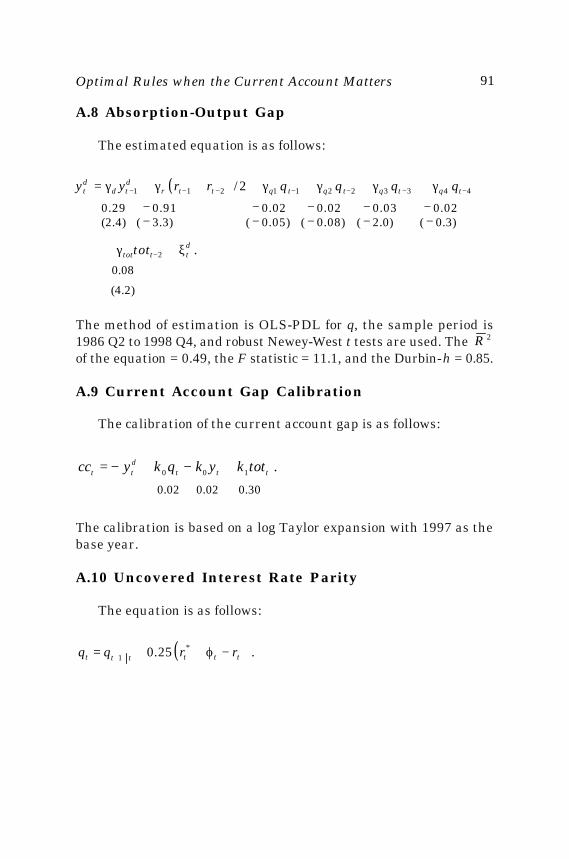
A.8 Absorption-Output Gap


The method of estimation is OLS-PDL for q, the sample period is1986 Q2 to 1998 Q4, and robust Newey-West t tests are used. The 2Rof the equation = 0.49, the F statistic = 11.1, and the Durbin-h = 0.85.

A.9 Current Account Gap Calibration

The calibration of the current account gap is as follows:

0.30 0.02 0.02

.100 tttdtt totkykqkycc +−+−=

The calibration is based on a log Taylor expansion with 1997 as thebase year.

A.10 Uncovered Interest Rate Parity

The equation is as follows:

( ) .25.01 tttttt rrqq −ϕ++= ∗+

( )

(4.2)

0.08

.

2/

2

4 43 32 21 1211

dtttot

tqtqtqtqttrdtd

dt

tot

qqqqrryy

ξ+γ+

γ+γ+γ+γ++γ+γ=

−

−−−−−−−

0.29 − 0.91 − 0.02 − 0.02 − 0.03 − 0.02(2.4) ( − 3.3) ( − 0.05) ( − 0.08) ( − 2.0) ( − 0.3)


APPENDIX B

State-Space Representation

This appendix shows how to write the model in the state-spaceform. As noted by Svensson (2000), given rational expectations, theinflation gap has the following behavior:

.111π+++ ξ+π=π tttt

Moreover, shifting the inflation equation one period forward and tak-ing expectations based on information up to time t, one arrives at anequation that can be solved for tt 3+π as a function of known variablesand of tt 2+π and tt 1+π . With these considerations one can write thematrix A of equation (15) in the following way:

( )[ ]

,

25025011

0

A

21

21

5419

18

17

18

13

13

11

10

9

20

7

6

19

5

4

2

1

41

−−λ−

ρρ

ρ+ρ

=

ϕ

AE

E.E.EE/

AE

EAEEEEEEE

EE

EE

EE

r

rtottot

.

.


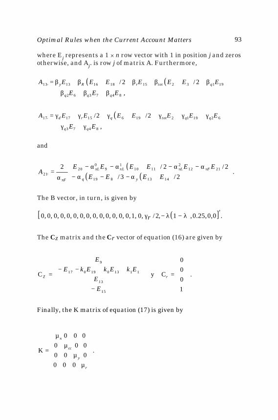
where Ej represents a 1 × n row vector with 1 in position j and zerosotherwise, and Aj. is row j of matrix A. Furthermore,

( ) ( ),

2/2/

847362

191321518161313

EEE

EEEEEEEA

qqq

qtotrRy

β+β+β+

β++β+β++β+β=

( ),

2/2/

8473

621912196151717

EE

EEEEEEEA

qq

qqtotqrd

γ+γ+

γ+γ+γ++γ+γ+γ=

and

( )( ) ( ) .

2/3/

2/2/2

1413819

21122

11101

90

2021

+α−−α−

α−α−+α−α−

α= ππππ

π EEEE

EEEEEEA

yq

FLLL

F

The B vector, in turn, is given by

( )[ ] .'0,0,25.0,1,2/ 0, 1, 0, 0, 0, 0, 0, 0, 0, 0, 0, 0, 0, 0, 0, 0, λ−λ−γr

The Cz matrix and the Cr vector of equation (16) are given by

.

1000

CyC

15

13

1113019017

9

=

−

++−−= rZ

EE

EkEkEkEE

Finally, the K matrix of equation (17) is given by

.

000000000000

K

µµ

µµ

=

π

r

y

cc

.

.

.


REFERENCES

Backus, D., and J. Driffill. 1986. “The Consistency of Optimal Policyin Stochastic Rational Expectations Models.” CEPR DiscussionPaper 124. London: Centre for Economic Policy Research.

King, M. 1999. “Challenges for Monetary Policy: New and Old.”Paper presented at a symposium on New Challenges for Mon-etary Policy, sponsored by the Federal Reserve Bank of Kan-sas City, August.

Magendzo, I. 1998. “Inflación e Incertidumbre Inflacionaria en Chile.”Economía Chilena 1(1): 29-42.

Massad, C. 1998. “La Política Monetaria en Chile.” Economía Chilena1(1): 7-27.

Medina, J. P., and R. Valdés. 2002. “Optimal Monetary Policy RulesUnder Inflation Range Targeting”. In this volume.

Ryan, C., and C. Thompson. 1999. “The Exchange Rate and MonetaryPolicy Rules.” Unpublished paper. Sydney: Reserve Bank ofAustralia (August).

Söderlind, P. 1999a. “Solution and Estimation of RE Macromodelswith Optimal Policy.” European Economic Review 43: 813-23.

. 1999b. “Algorithms for RE Macromodels with Optimal Policy-Lecture Notes.” Unpublished paper. Stockholm: Stockholm Schoolof Economics.

Svensson, L. E. O. 1994. “Why Exchange Rate Bands? Monetary In-dependence in Spite of Exchange Rate Bands.” Journal of Mon-etary Economics 33(1): 157-99.

. 1999. “How Should Monetary Policy Be Conducted in anEra of Price Stability?” Paper presented at a symposium on NewChallenges for Monetary Policy, sponsored by the Federal Re-serve Bank of Kansas City, August.

. 2000. “Open-Economy Inflation Targeting.” Journal of In-ternational Economics 50: 155-83.

Woodford, M. 1999a. “Optimal Monetary Policy Inertia.” NBER Work-ing Paper 7261. Cambridge, Mass.: National Bureau of EconomicResearch.

. 1999b. “Commentary: How Should Monetary Policy Be Con-ducted in an Era of Price Stability?” Paper presented at a sympo-sium on New Challenges for Monetary Policy, sponsored by theFederal Reserve Bank of Kansas City, August.

Optimal MOnetary Policy Rules when the Current Account Matters

Documents

Transcript of Optimal MOnetary Policy Rules when the Current Account Matters