Operational planning of herbicide-based weed management

1

OPERATIONAL PLANNING OF HERBICIDE-BASED WEED MANAGEMENT 1

2

Mariela V. Lodovichia*, Aníbal M. Blanco

b, Guillermo R. Chantre

a , J. Alberto Bandoni

b, Mario 3

R. Sabbatinia, Mario Vigna

c, Ricardo López

c, Ramón Gigón

c4

5

aDepartamento de Agronomía/CERZOS, Universidad Nacional del Sur/CONICET, Bahía Blanca 6

(8000), Buenos Aires, Argentina. 7

8

bPlanta Piloto de Ingeniería Química, Universidad Nacional del Sur/CONICET, Bahía Blanca 9

(8000), Buenos Aires, Argentina. 10

11

cEEA INTA Bordenave, Bordenave (8187), Buenos Aires, Argentina. 12

13

*Corresponding author: Mariela V. Lodovichi, Departamento de Agronomía, Universidad14

Nacional del Sur, Av. Colón 80, Bahía Blanca (8000), Argentina. Tel: +54 – 291 – 4595102; 15

Fax: 54 – 291 – 4595127. E-mail: [email protected] 16

Authors’ e-mail addresses: [email protected] (A.M. Blanco), [email protected] 17

(G.R.Chantre), [email protected] (J.A. Bandoni), [email protected] (M.R. 18

Sabbatini), [email protected] (M. Vigna), [email protected] (R. 19

López), [email protected] (R. Gigón) 20

21

22

23

24

25

26

27

28

29

30

mailto:[email protected]








http://ees.elsevier.com/agsy/viewRCResults.aspx?pdf=1&docID=4751&rev=0&fileID=98074&msid=D479D5BF-2061-4DA0-A366-FDAB7F56F281

2

Abstract 31

32

Weeds cause crop yield loss due to competition, interfere with agronomic activities and reduce 33

grain quality due to seed contamination. Among the numerous methods for weed control, the 34

use of herbicides is the most common practice. Nowadays, the optimization of herbicide 35

application is pursued to reduce the environmental impact, delay the appearance of herbicide-36

resistant weed populations, and improve the cost/benefit ratio of the agronomic business. This 37

work proposes an operational planning model, aimed at calculating the optimal application times 38

of herbicides in no-tillage systems within an agronomical season in order to maximize the 39

economical benefit of the activity while rationalizing the intensity of the applications with respect 40

to expert knowledge based recommendations. The model can decide on herbicide applications 41

on a daily basis, consistent with timing of agronomic activities, and provides an explicit 42

quantification of the environmental impact as an external cost. The proposed approach was 43

tested on a winter wheat (Triticum aestivum) - wild oat (Avena fatua) system, typical of the 44

semiarid region of Argentina. In all the studied scenarios at least two pre-sowing applications of 45

non-selective herbicides were required to effectively control early emerging weed seedlings. 46

Additional pre-sowing and post-emergence applications were also advised in cases when 47

competitive pressure was significant. 48

Keywords 49

Weed management, planning model, herbicide applications, environmental impact, winter 50

wheat, wild oat 51

52

53

1. Introduction 54

55

Weed control in crops is mainly based on the use of herbicides because they are efficient and 56

easily applied. However, nowadays, attempts are made to minimize the use of chemicals in 57

order to mitigate environmental impact and to avoid the appearance of herbicide-resistant weed 58

populations. The optimization of weed control is largely recognized to be a challenging and 59

information demanding task. As asserted in Wiles et al. (1996): “Ideally a decision maker should 60

3

know the emergence patterns of the weed, the crop’s ability to suppress weed growth, the effect 61

of different weed species on crop yield and quality, and characteristics of possible management 62

options”. 63

64

In order to integrate the available information and systematically explore weed control options, 65

several model-based decision support systems (DSS) have been developed in the last years. In 66

Table 1, some of such works are summarized. The review is not intended to be exhaustive but 67

rather to present an outlook of the developed DSS strategies. The approaches are presented in 68

tabular fashion to broadly describe their main characteristics, modeling features and devised 69

purposes. 70

71

Since weeds have specific agro-ecological adaptations, the DSSs are not supposed to be used 72

beyond their design scope, without proper adjustments. Therefore, in all cases the studied 73

weed/crop system is reported together with the country (or region within a country) of origin 74

(Table 1). Moreover, major modeling components, classified as climatic, biological and 75

economic, are also identified. The climatic component makes reference to an explicit use of 76

weather data, while the biological component reflects the quantitative modeling of some of the 77

most important eco-physiological sub-processes (emergence, seedling survival, seed 78

production, etc.). This component is further classified as empirical or mechanistic, making clear 79

that the mechanistic approach makes use, in general, of some amount of empirical information. 80

81

By inspecting Table 1, it can be observed that most DSSs are devoted to typical annual weeds 82

in wheat based rotations. Most systems were also designed in European countries although it is 83

evident that the automation of the weed control management is of worldwide interest. Regarding 84

the type of biological model, most systems are based on dynamic population balances (i.e., 85

seeds present in the seedbank, emerged seedlings, surviving of mature plants) whose flows are 86

described through empirical parameters. In the cases where the biology is more mechanistically 87

represented (Colbach et al., 2007; Parsons et al., 2009) weather data is also required. 88

89

4

Economic balances are also performed in most DSSs in order to evaluate the potential profit of 90

implementing different control procedures. Regarding the evaluation approach, most systems 91

are designed to be used in a simulation oriented fashion, meaning that a certain strategy is 92

proposed and its effect on the weed-crop system is calculated. In this way, different possible 93

scenarios can be tested and ranked according to their economic output. However, due to the 94

fact that the feasible control combinations on a long term time-horizon (i.e. several seasons, 95

considering chemical and non-chemical control treatments) are considerably extensive, some 96

DSSs also implement numerical optimization algorithms to automate the search. 97

98

Regarding the scope of application, the conducted research on DSS development has been 99

basically focused on the tactical/strategic planning problem, which addresses the weed control 100

decisions over a long-term horizon of several years. In this regard, the DSSs divide the seasons 101

into periods of biological and agronomic sense, rather than using a daily step, to perform the 102

calculations and implement the control operations. Finally, although all the DSSs are designed 103

to rationalize the chemical use and mitigate the environmental impact of weed control, only two 104

models explicitly perform some quantitative evaluation of an environmental impact related 105

indicator. Specifically, in Berti et al. (1997, 2003) the potential contamination of groundwater is 106

considered, while in Falconer and Hodge (2001) the impact of pesticides application is analyzed 107

within a bi-objective (economic-environmental) optimization approach. 108

109

Table 1 (near here) 110

111

From the above review, it can be stated that the contributions are basically focused on the 112

tactical/strategic planning problem. To the best of our knowledge, no proposals related to the 113

herbicide selection problem integrated with the calculation of the optimal application times have 114

been presented so far. Such short-term problem can be considered as an “operational planning” 115

problem of the agronomic activity. The importance of the operational planning perspective relies 116

on the fact that if herbicide applications are made too soon, later emergence will require 117

additional interventions for effective control, incurring in additional costs and environmental 118

5

impact. On the other hand, if the herbicide applications are delayed, the older weeds might 119

survive, competing with the crop and producing new seeds. 120

121

The main difficulty related to the operational planning of herbicide based weed control is that the 122

emergence pattern of the weed is uncertain. It is well known that in order to make an efficient 123

use of herbicides, an accurate prediction of the relative time of weed seedling emergence and 124

density is essential (Forcella et al., 2000). It should be pointed out that an accurate estimation of 125

weed emergence dynamics is a challenging goal since emergence onset and magnitude 126

depend on weather conditions, usually described in terms of hydrothermal time accumulation, 127

and are also modulated by complex adaptative seed dormancy traits, as stated by Chantre et al. 128

(2012, 2013) for wild oat. 129

130

This work proposes a conceptual operational planning model whose main features are 131

summarized in the last row of Table 1. The system wild oat (Avena fatua) – winter wheat 132

(Triticum aestivum), typical of the semiarid region of Argentina, is used as a case study. The 133

aim is to maximize the economic benefit of the agronomic activity with explicit consideration of 134

the environmental impact, through the selection of the proper herbicides and the corresponding 135

application times in a no-tillage system along the agronomical season. 136

137

2. Materials and Methods 138

139

2.1. Crop yield loss 140

141

Crop yield loss (yL) caused by competition with a single weed species has been described by 142

the rectangular hyperbola model of Cousens (1985): 143

144

a

i1

i

D

Dy L

(1) 145

where D is weed density in plants m-2

, and i and a are model parameters. Parameter i is the 146

percent yield loss per weed plant per unit area as weed density approaches zero and parameter 147

6

a is the upper limit of percent yield loss as weed density approaches infinity. Eq. (1) assumes 148

that all weed plants present in the field emerge simultaneously with the crop and compete with it 149

until harvest. 150

151

As yield loss cannot be observed directly, the final yield of the crop (y) has to be estimated as a 152

proportion of the weed-free crop yield (ywf) in kg ha-1

, through the following relation: 153

154

1001ywf

Lyy (2) 155

156

Since weed seedlings do not usually emerge simultaneously with the crop, the final weed 157

density is in general not adequate to calculate the actual yield loss. In fact, seedlings that 158

emerge earlier in the season cause greater yield losses than those that emerge later. Cousens 159

et al. (1987) modified model (1) to include the relative emergence time of the weed as a 160

parameter: 161

162

a

be

b

cRT D

DyL

(3) 163

164

where RT is the time interval between weed emergence and crop emergence, b is the value of i 165

when RT = 0 and c is the rate at which i decreases as RT becomes larger. RT is negative if 166

weed seedlings emerge earlier than the crop and positive if the crop emerges first. 167

168

This approach still considers that all weed seedlings emerge simultaneously. However, in 169

nature field emergence patterns are mostly determined by successive cohorts which impact on 170

crop yield differently depending on relative emergence time. Based on equation (3) Berti et al. 171

(1996) proposed the use of the concept of “time-density equivalent” (TDE) to consider both, 172

seedling emergence time and relative emergence, on the estimation of crop yield loss. For 173

weed seedlings with a given emergence time, TDE can be defined as the density of a reference 174

weed that emerges uniformly and competes with the crop until harvest causing the same yield 175

7

loss as that incurred by the actual weed. Weeds emerging earlier have a larger TDE than those 176

emerging later. TDE of each daily cohort is calculated as: 177

178

TDEt = D exp(-c RTt) (4) 179

180

In this work we used the concept of TDE to account for the effect of weed cohorts (i.e. seedlings 181

emerging at different moments). TDE was calculated in a daily basis, and then integrated to 182

obtain a global TDE. This global TDE was used instead of weed density (D) to estimate crop 183

yield loss in equation (1). 184

185

2.2. Pesticide Environmental Accounting (PEA) 186

187

To account for the environmental impact of pesticides use, Leach and Mumford (2008) 188

developed a methodology to estimate the associated external costs. External costs include 189

monitoring for contamination of soil, water and food, and poisoning of humans and fauna. Such 190

costs are usually absorbed by society and, therefore, not taken into account in individual 191

decision making so far. The approach by Leach and Mumford is based on the Environmental 192

Impact Quotient (EIQ) (Kovach et al., 1992). The EIQ describes the environmental impact of a 193

pesticide in terms of an eco-toxicological quotient. The EIQ is calculated for each pesticide 194

considering eight categories: toxicological effects on pesticide applicators, pickers and 195

consumers, ground water contamination, aquatic effects and toxicological effects on birds, bees 196

and beneficial insects. 197

198

PEA provides the external cost per kg of active ingredient of an average pesticide. This external 199

cost is distributed into the eight EIQ components. Each category is classified as having low, 200

medium or high impact according to corresponding EIQ values and the external cost is weighted 201

by a coefficient of 0.5, 1.0 or 1.5 respectively. These external costs are then adjusted for each 202

chemical by the active ingredient concentration on the formulated (or commercial) product and 203

by the field application rate for each chemical. External costs calculated by PEA (in Euros ha-1

204

application-1

) are based on average estimations from the United Kingdom, the United States of 205

8

America and Germany. To adapt this calculation to Argentina, the external costs were scaled to 206

the Argentinean Gross Domestic Product (GDP) as a proportion of the average GDP of the 207

reference countries according to the approach proposed in Leach and Mumford (2008). PEA 208

was applied to the specific case of herbicides use in sugar beet systems in Leach and Mumford 209

(2011). 210

211

2.3. Planning model development 212

213

The developed planning model is presented below. It was built on the previously described 214

elements and structured within the frame of a multi-period mathematical programming 215

formulation. A one year time horizon with a daily time step was considered for modeling 216

purposes, in order to account for the typical agronomical cycle and data availability frequency. 217

The model provides the optimum weed control strategy by selecting which herbicide to apply 218

each period of the planning horizon. For a complete description of model variables and 219

parameters see Tables 2 and 3. 220

221

2.3.1. Weed density estimation 222

223

The model predicts the evolution of weed density during the planning horizon. The number of 224

plants per square meter present in the system on day t is the sum of plants in all growth stages. 225

Density (Dt) is calculated as a plant balance among the number of seedlings emerged on day t 226

(Et) plus the weed density on the previous day (Dt-1) minus the seedlings eliminated by control 227

operations performed on day t (Mt): 228

229

Dt = Dt-1 + Et - Mt t (5) 230

231

2.3.2. Weed plants mortality 232

233

Weeds can be effectively controlled only if the plants are on the appropriate growth stage. It is 234

assumed that weed seedlings are killed only by herbicides applications, and that all susceptible 235

9

individuals present in the day of the application are effectively controlled (i.e. 100% efficiency). 236

The model calculates the number of weed plants killed by each available treatment at day t 237

(Mtht,h) as follows: 238

239

Mtht,h ≤ ∑ t- nsh2(h) ≤ t1 ≤ t-nsh1(h) EMtt1,h + bigM (1 - yhtht,h) t, h (6) 240

Mtht,h ≥ ∑ t- nsh2(h) ≤ t1 ≤ t-nsh1(h) EMtt1,h - bigM (1 - yhtht,h) t, h (7) 241

Mtht,h ≤ yhtht,h bigM t, h (8) 242

243

yhtht,h is a binary variable that is equal to 1 if herbicide h is applied on day t or becomes zero 244

otherwise. bigM is a large constant that represents an upper level for variable Mtht,h. Eqs. (6)-245

(8) constitute a big-M formulation which enforces that the number of killed plants is equal to 246

the number of plants on the proper growth stage if a herbicide application takes place, and that 247

it is equal to zero otherwise. 248

249

EMtt,h, also defined through a big-M formulation, is equal to Et if the weed seedlings emerged on 250

day t are killed by an application of herbicide h during their period of susceptibility and is zero 251

otherwise: 252

253

EMtt,h ≥ Et – bigM (1 - bight,h) t, h (9) 254

EMtt,h ≤ Et + bigM (1 - bight,h) t, h (10) 255

EMtt,h ≤ bigM bight,h t, h (11) 256

257

bight,h is a positive variable that integrates the number of herbicide applications made during the 258

susceptibility period of weed seedlings emerged on day t: 259

260

bight,h = ∑ t+nsh1h ≤ t1 ≤ t+nsh2h yhtht1, h t, h (12) 261

262

The total number of plants controlled on day t is calculated by integrating the plants controlled 263

by each particular herbicide that day: 264

265

10

Mt = ∑h Mtht,h t (13) 266

267

2.3.3. Estimation of crop yield loss and final crop yield 268

269

As mentioned above, the model adopts the TDE approach to calculate crop yield loss, in order 270

to account for the impact of weed emergence time on competition. To obtain the daily TDE 271

(TDEt) it was necessary to consider only those plants that would continue in the system until 272

harvest. For weed seedlings emerged on day t, Ettt is defined as those plants that are not killed 273

by any herbicide application, and is calculated as follows: 274

275

Ettt = Et - ∑ h EMtt,h t (14) 276

277

Ettt represents the daily density incorporated to the system. This variable replaces D in equation 278

(4) to calculate the daily TDE: 279

280

TDEt = Ettt exp(-c RTt) (15) 281

282

RTt is the relative time of emergence of weed seedlings emerged on day t with respect to the 283

crop. For each day on the planning horizon, it is calculated as: 284

285

RTt = Temt – Dec (16) 286

287

Temt is a parameter that represents the date of weed seedling emergence on day t, and Dec is 288

the day of crop emergence. Dec is calculated from sowing date (Des) and the time period from 289

sowing to crop emergence (Tec) as: 290

291

Dec = Des + Tec (17) 292

293

11

The global TDE (TDEtot) represents the total number of weed plants that will be present in the 294

system until crop harvest and will be responsible for crop yield loss. It is then calculated as 295

follows: 296

297

TDEtot = ∑t TDEt (18) 298

299

This global TDE replaces D in equation (1) to estimate the impact that these plants have on 300

crop yield. yL is obtained as a percentage of the potential yield that the crop could produce: 301

302

a

i1

i

TDEtot

TDEtotyL

(19) 303

304

Finally, it is necessary to calculate the final crop yield (y) to estimate the profit obtained at the 305

end of the season using eq. (2): 306

307

1001ywf

Lyy

(20) 308

309

2.3.4. Objective function 310

311

The herbicide application planning problem is formulated as an optimization model aimed at 312

maximizing the economical benefit (B) of the agronomical activity. The proposed objective 313

function considers an income term (Inc) related to the predicted crop yield, a cost term (Cost) 314

related to control operations (herbicide applications) and the environmental costs (Ext) of the 315

applied chemicals: 316

317

B = Inc – Cost – Ext (21) 318

319

The gross income at the end of the season depends on the final crop yield (y) and on the price 320

of the grain (pc). It is calculated as follows: 321

12

322

Inc = pc . y (22) 323

324

The application cost of the herbicides is calculated from the cost of each individual application: 325

326

Cost = ∑ h costhh (∑t yhtht,h) (23) 327

328

where costhh is the cost in $ ha-1

of one application of herbicide h. 329

330

Finally, the environmental cost (Ext) associated to herbicide applications is calculated as a 331

function of the external cost of each application (PEAh) performed by the model: 332

333

Ext = ∑ t (∑ h yhtht, h PEAh) (24) 334

335

2.3.5. Herbicides 336

337

Non-selective herbicides are available to control weeds before crop sowing, in order to early 338

eliminate plants with a great competitive advantage. Selective herbicides are available for weed 339

control purposes after the crop’s susceptibility period. Restrictions were included to avoid 340

spraying operations in periods were the different herbicides cannot be applied. Constraint (25) 341

avoids the application of non-selective herbicides after sowing: 342

343

yhtht, h = 0 t ≥ Des, hns (25) 344

345

Constraint (26) prevents the application of selective herbicides before sowing and during crop’s 346

susceptibility period: 347

348

yhtht, h = 0 t ≤ Dec+ns, hs (26) 349

350

13

Eq. (27) avoids the application of a selective herbicide more than once in the season. This is a 351

“heuristic” constraint to mimic a practice intended to mitigate the manifestation of weed 352

resistance in the long term and to avoid crop phytotoxicity. 353

354

∑ t yhthh,t ≤ 1 hs (27) 355

356

The GAMS platform and the solver Dicopt++ (GAMS 2008 a, b) were used to program and 357

solve the resulting mixed integer non-linear model. 358

359

360


362

363


365

366


368

3. Results and Discussion 369

370

3.1. Scenario analysis 371

372

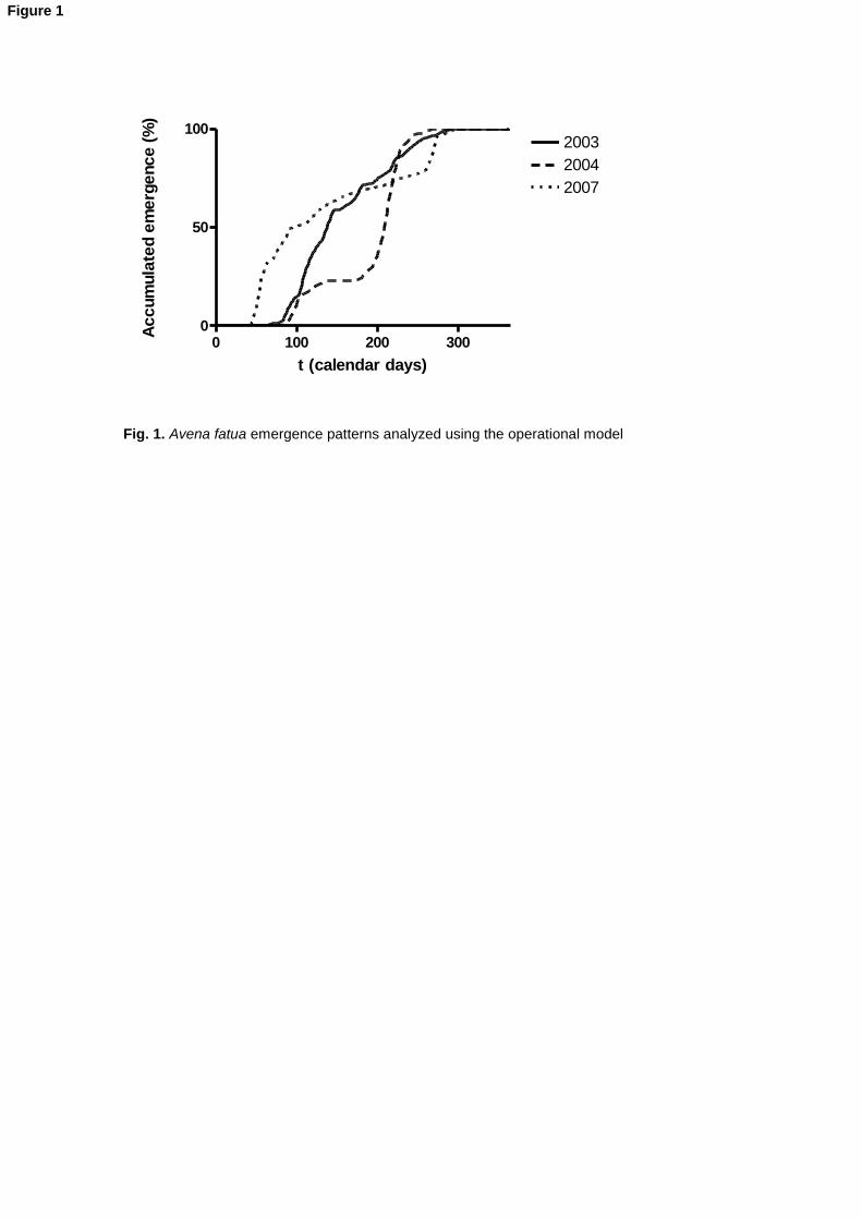
Avena fatua seedling emergence in the semiarid region of Argentina is difficult to predict 373

because it is strongly influenced by uncertain weather conditions (i.e. precipitations and 374

temperature) and highly modulated by seed-bank dormancy behavior (Chantre et al. 2012). In 375

this work, three different seedling emergence patterns registered at Experimental Station of 376

INTA at Bordenave, Argentina (37⁰50’ S; 63⁰01W) were used to test the proposed model. 377

These patterns were selected according to the time taken to reach 50% of the total emergence, 378

and are considered representative of the variability observed in the region under study. The 379

chosen scenarios correspond to years 2003 (Case 1), 2004 (Case 2) and 2007 (Case 3), where 380

14

50% of emergence was reached after 145, 215 and 110 calendar days, respectively (Fig. 1). A 381

non-dormant seed bank of 200 seeds m-2

was adopted for the base case scenario analysis. 382

383

The model parameters for the Triticum aestivum – Avena fatua system are reported in Table 2. 384

Some parameters were obtained from the literature (Cousens, 1985; Cousens et al., 1987) and 385

the others estimated from authors’ personal experience on the particular system. Eight different 386

active ingredients, commonly used for Avena fatua control in Argentina, were considered in this 387

case study. In Table 4, two non-selective pre-sowing herbicides and six selective post 388

emergence herbicides are depicted. Each herbicide has different application and environmental 389

costs and periods of weed and crop susceptibility. They were all considered as sprayed at label 390

dose recommendations. The details of the PEA calculation for each particular herbicide are 391

provided in Appendix A. 392

393

Figure 1 (near here) 394

395

396


398

Optimization results indicate that in Case 1 (Fig. 2), where 50% of wild oat emergence was 399

reached a few days before sowing, the maximum benefit was obtained after three pre-sowing 400

glyphosate treatments, and one post-emergence application of pyroxsulam. These applications 401

controlled more than half of the seedlings emerged during the considered planning horizon. 402

Although after the last application final weed density increased, the number of plants affecting 403

crop yield loss remained constant. Final weed density was 61 plants m-2

, but only 18 individuals 404

had a significant impact on final crop yield (Table 5). 405

406

In Case 2 (Fig. 3), the model proposed only two glyphosate applications in crop pre-emergence. 407

These applications were sufficient to control the few plants emerged during that period. 408

Because most weed seedlings emerged long after sowing, their impact on crop yield was not 409

significant and it would not be optimal to perform any post-emergence control action. Fig. 3 410

15

shows that although after those applications final weed density was 154 plants m-2

, only 2% of 411

the individuals actually impacted on crop yield (Table 5). 412

413

Finally, in Case 3 (Fig. 4), where 50% of emergence was reached long before sowing, three 414

applications of glyphosate were required. In this case, final weed density was 72 plants m-2

from 415

which 23 plants m-2

were responsible for the predicted crop yield loss (Table 5). Although after 416

the last application global TDE increased considerably, those plants were not controlled 417

because the post-emergence herbicide should have been applied during the crop susceptibility 418

period. 419

420

By analyzing the studied scenario it is evident that early emergent weed cohorts, which has a 421

large impact on crop yield, requires several pre sowing herbicide applications to control wild oat 422

infestation in all cases. If emergence is too early (Case 3), only pre sowing treatments are 423

required because all potentially competitive weeds are removed at this stage. If weed 424

emergence is considerably delayed (Case 2), weed seedlings emerging after crop 425

establishment do not have a significant effect on cereal yield and additional applications are not 426

required. The most challenging scenario arises when a large proportion of the weed emergence 427

is overlapped with the crop susceptibility period (Case 1). In this case, some post-emergence 428

control action is required to avoid excessive competitive pressure on the crop. 429

430

In the absence of control operations, the analyzed emergence patterns would have led to a 431

great infestation. Considering that Avena fatua is a strong competitor and can reduce crop yield 432

to around 100%, the control treatments proposed by the model were capable of reducing crop 433

yield losses to less than 15% in all cases. The environmental costs of herbicide applications 434

were considered in the objective function for the three emergence scenarios. In all cases these 435

values were much lower than the corresponding application costs and therefore had not shown 436

a considerable impact on the choice of the control strategies. 437

438

The performance of more than one application of glyphosate during the same season might be 439

considered as a non-recommendable practice because it represents a strong pressure on weed 440

16

populations that may lead to increase herbicide resistance rate. The use of the alternative non-441

selective ingredient (i.e. Paraquat) was never advised by the model due to its high relative cost 442

with respect to glyphosate. In the cases where glyphosate was constraint to be applied only 443

once along the season, negative benefits were obtained due to an unfavorable balance 444

between control costs and cereal yields (results not shown). However, in the region under 445

study, it is a common practice to repeat glyphosate applications during fallow due to necessity 446

of control of many problematic gramineous and broad-leaved weeds. 447

448

The advice given by the model of whether to apply or not the graminicide is of great practical 449

importance. This decision is one of the most difficult to make because each herbicide 450

application is expensive, and it is of great practical interest for the producer or agronomic 451

advisor to know if it is worth to implement it. 452

453


455


457


459

460


462

3.2. Sensitivity analysis 463

464

The model parameters were assumed constant in the scenario analysis but most of them have 465

a significant level of uncertainty. In order to assess the impact of parameters uncertainty on 466

model outputs, some parameters were varied individually to some extent. Specifically, the 467

sensitivity to the seed bank size and the weed susceptibility period to herbicides is reported 468

using the emergence pattern corresponding to year 2003 (Case 1) as base case scenario. 469

17

470

In Table 6 the sensitivity of most relevant variables with respect to the seed bank size is 471

presented. For increasing number of seeds in the seed bank it can be observed that the 472

application strategy did not change significantly, since three pre-sowing applications of 473

glyphosate and one post-emergence application of pyroxsulam took place approximately in the 474

same periods for all cases. Interestingly, larger benefits are observed for larger seed banks 475

(+10 and +20 %) with respect to the base case only due to the shifts in the periods of 476

application. For the 25% increased seed bank, the application strategy could not compensate 477

the weed competitive pressure and a reduced crop yield was obtained with respect to the base 478

case. 479

480

As expected, for decreasing seed banks, larger benefits with respect to the base case were 481

obtained in all scenarios. For the -10 and -25 %, the application program is the same as in the 482

base case, with minor variations in the glyphosate application periods. However, in the -20% 483

case, only the three pre-sowing glyphosate applications were required, with no post emergence 484

intervention. Although a large crop yield loss took place in this situation (14.9%), significantly 485

reduced control costs compensated the income decrease, producing a larger benefit than in the 486

base case. 487

488


490

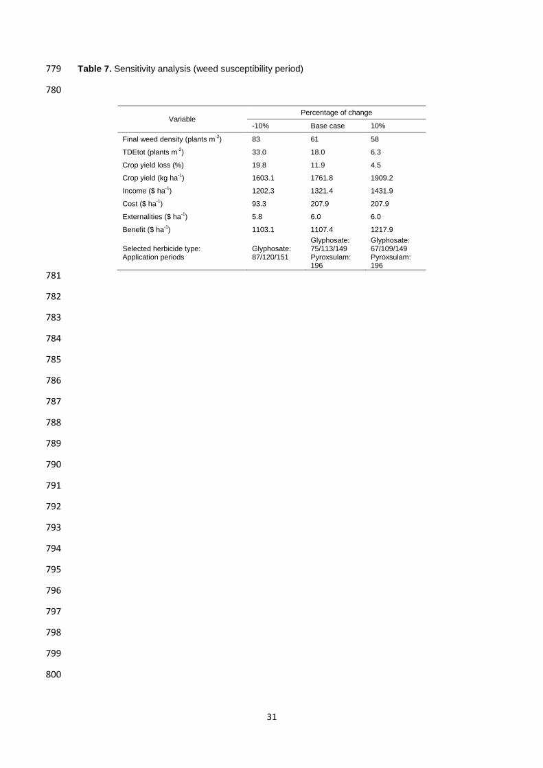
In Table 7 the sensitivity of the solution with respect to the susceptibility period of the weed to 491

the herbicides is presented. The susceptibility to all herbicides was modified simultaneously in 492

order to simulate environmental conditions that enlarges and reduces the control period of the 493

herbicides. For example, in the +10% case, nsh1h was reduced in 10% and nsh2 h incremented 494

in 10% enlarging the effectiveness periods of the herbicides. In this case, the control solution 495

remains the same as in the base case (three pre-sowing and one post-emergence treatment) 496

with some shifts in the pre-sowing applications. However, the enlarged control action of the 497

herbicides allowed a significant reduction in TDE tot (64.83%) which produced a larger cereal 498

yield with the consequent benefits. 499

18

500

A reduced herbicide efficiency (-10% case) provided an optimal treatment with only three pre-501

sowing applications and no post emergence control. The application times of the first two 502

controls were quite delayed regarding the base case in order to better control the emergent 503

weed. Although the crop yield loss increased regarding the base case, the reduced costs 504

compensated for the reduced benefits in the economic equation and only a 0.38% decrease of 505

the total profit with respect to the base case solution was observed. 506

507

By analyzing the sensitivity study it can be concluded that the solutions are quite robust in the 508

sense that basically the same treatment is obtained in most cases (three pre-sowing and one 509

post-emergence applications). The major variations are found in the application timing. By 510

adequate shifts in the application periods, the model is able to compensate for unfavorable 511

situations (i.e. increased seed banks) or to exploit favorable conditions (i.e. enlarged 512

susceptibility periods) without changing the overall herbicides combination. In the cases where 513

post emergence applications were not required (20% seed bank reduction and 10% 514

susceptibility period reduction) significant crop yield losses were compensated in both cases by 515

the a reduction of costs due to one less chemical application. 516

517

4. Conclusions and future work 518

519

The model proposed in this work automates the calculation of the optimal application times of 520

herbicides within an agronomical season. These times depend on the estimated weed 521

emergence pattern, which in turn depends on the degree of dormancy of the seeds present in 522

the seed bank and on the climatic conditions (Forcella et al., 2000). The emergence pattern was 523

treated as a single parameter in the model in order to comprise both, the biological and the 524

climatic components involved in weed emergence. If available, sub-models that relate weed 525

emergence with weather forecasts can be used. Many of these have been developed in the last 526

years for different systems (Forcella el al., 2000; Chantre et al., 2012, 2013). 527

528

19

One of the most challenging aspects was the calculation of crop yield loss according to weed 529

density. Because those weed plants that emerge earlier are more influential in competition, in 530

this work they were weighted according to their emergence time. Therefore, although the final 531

weed density is over-estimated by the model, since it considers that weeds keep emerging even 532

when the crop is already in an advanced phenological stage, the competitive influence of these 533

late emerging plants has not a significant effect on cereal yield. However, in order to make a 534

more realistic calculation, both, age and permanence in the system should be considered. 535

Moreover, the competition for nitrogen, light and water might be addressed through the 536

mechanistic modeling of the crop-weed interactions (Kropff and Van Laar, 1993). 537

538

As mentioned above, the developed model is operational in nature, meaning that only short 539

term (seasonal) decisions are considered. Moreover, only chemical control options at the 540

recommended label doses were included in the present version. Many other control methods 541

exist that should be taken into account from a strategic point of view. The importance of 542

strategic weed control planning has been largely recognized in order to account for the long-543

term effects of crop rotations and mechanical and cultural controls on weed infestation levels 544

and manifestation of chemical resistant biotypes (Pannell et al., 2003; Parsons et al., 2009). In 545

this sense the proposed model can be considered as the seasonal module of the chemical 546

control within a strategic planning system. 547

548

Practically every model parameter presents a significant uncertainty, specifically those that 549

somehow depend on climatic conditions. Sensitivity analysis on most influential parameters 550

revealed interesting behaviors, suggesting that uncertainty should be explicitly handled in real 551

applications. A practical solution could be to run the model within a model predictive control 552

framework in order to identify the short term optimal solution with the available weather forecast 553

and recalculate a new forehead solution as a new forecasts become available, taking into 554

account the already implemented control actions (Ogunnaike and Ray, 2000) 555

556

Finally, the PEA methodology was chosen among the environmental impact evaluation 557

approaches because it allowed straightforwardly including the environmental component as an 558

20

externality in the model objective function to account for the environmental impact of the 559

herbicides application. This inclusion did not produce a significant impact on the model output 560

since external costs per application of any of the herbicides considered is much lower than 561

application costs. However, the explicit inclusion of an environmental component in economic 562

terms is practical to quantify the effect of the different available chemical options and to highlight 563

the environmental concern during the agronomical decision making process. 564

565

If alternative environmental impact indicators, not formulated in economic terms, are to be 566

analyzed, a multi-objective approach should be adopted to study the trade-off between 567

maximizing the economical benefit and minimizing the environmental impact. 568

569

Acknowledgements 570

571

This work was partially supported by: Consejo Nacional de Investigaciones Científicas y 572

Técnicas (CONICET PIP Nº 11220100100222), Agencia Nacional de Promoción Científica y 573

Técnica and Universidad Nacional del Sur (Argentina) (PGI 24/A157). We are also grateful to 574

Eng. Jorge Irigoyen (in memoriam) for expert advice and fruitful discussions. 575

576

References 577

578

Berti, A., Dunan, C., Sattin, M., Zanin, G., Westra, P., 1996. A new approach to determine 579

when to control weeds. Weed Sci. 44, 496-503. 580

Berti, A., Zanin, G., 1997. GESTINF: a decision support model for post-emergence weed 581

management in soybean (Glycine max (L.) Merr.). Crop Prot. 16, 109-116. 582

Berti, A., Bravin, F., Zanin, G., 2003. Application of decision-support software for 583

postemergence weed control. Weed Sci. 52, 618-627. 584

CASAFE, 2007. Guía de productos fitosanitarios. Tomo II. Generalidades y productos para la 585

República Argentina. Cámara Argentina de Sanidad Agropecuaria y Fertilizantes (CASAFE), 586

Argentina. 587

21

Chantre, G., Blanco, A.M., Lodovichi, M.V., Bandoni, J.A., Sabbatini, M.R., Vigna, M., López, 588

R., Gigón, R., 2012. Modeling Avena fatua seedling emergence dynamics: an artificial neural 589

network approach. Comput. Electron. Agr. 88, 95-102. 590

Chantre G. R., Blanco, A.M., Forcella, F., Van Acker, R.C., Sabbatini, M.R., Gonzalez-Andujar, 591

J.L., 2013. A comparative study between Nonlinear Regression and Artificial Neural Network 592

approaches for modeling wild oat (Avena fatua) field emergence. J. Agr. Sci. (in press). 593

Colbach, N., Chauvel, B., Gauvrit, C., Munier-Jolain, N. M., 2007. Construction and evaluation 594

of ALOMYSYS modelling the effects of cropping systems on the blackgrass life-cycle: From 595

seedling to seed production. Ecol. Model. 20I, 283-300. 596

Cousens, R., 1985. A simple model relating yield loss to weed density. Ann. App. Biol. 107, 597

239-252. 598

Cousens, R., Doyle, C. J., Wilson, B. J., Cussans G. W., 1986. Modelling the Economics of 599

Controlling Avena fatua in winter wheat. Pestic. Sci. 17, 1-12. 600

Cousens, R., Brain, P., O’Donovan, J.T., O’Sullivan, P.A., 1987. The use of biologically realistic 601

equations to describe the effects of weed density and relative time of emergence on crop 602

yield. Weed Sci. 35, 720-725. 603

De Buck, A.J., Schoorlemmer, H.B., Wossink, G.A.A., Janssens, S.R.M., 1999. Risks of post-604

emergence weed control strategies in sugar beet: development and application of a bio-605

economic model. Agr. Syst. 59, 283-299. 606

Doyle, C.J., Cousens, R., Moss, S.R., 1986. A model of the economics of controlling Alopecurus 607

myosuroides Huds. in winter wheat. Crop Prot. 5, 143-150. 608

EXTOXNET. Available from: http://pmep.cce.cornell.edu/profiles/extoxnet/ . Date of last access: 609

December 2012. 610

Falconer K., Hodge, I., 2001. Pesticide taxation and multi-objective policy making: farm 611

modeling to evaluate profit/environment trade-offs. Ecol. Econ. 36, 263-279. 612

Forcella, F., Benech-Arnold, R.L., Sanchez, R., Ghersa, C.M., 2000. Modeling seedling 613

emergence. Field Crop Res. 67, 123-139. 614

GAMS. 2008a. A Users’ Guide. GAMS Development Corporation 615

GAMS. 2008b. The Solvers Manual. GAMS Development Corporation 616

http://pmep.cce.cornell.edu/profiles/extoxnet/

22

González-Andújar, J.L., Fernández-Quintanilla, C., 1991. Modelling the population dynamics of 617

Avena sterilis under dry-land cereal cropping systems. J. Appl. Ecol. 28, 16-27. 618

González-Andújar, J.L., Fernández-Quintanilla, C., 2004. Modelling the population dynamics of 619

annual ryegrass (Lolium rigidum) under various weed management systems. Crop Prot. 23, 620

723-729. 621

IPM Center. Available from: http://www.ipmcenters.org/ecotox/ . Date of last access: December 622

2012. 623

Kovach, J., Petzold, C., Degnil, J., Tette, J., 1992. A Method to measure the environmental 624

impact of pesticides. New York’s Food and Life Sciences Bulletin 139, 1-8. 625

Kropff, M. J., van Laar, H. H., 1993. Modelling Crop-Weed Interactions, CAB International, 626

United Kingdom. 627

Leach, A. W., Mumford, J. D., 2008. Pesticide Environmental Accounting: A method for 628

assessing the external costs of individual pesticide applications. Environ. Pollut. 151, 139-147. 629

Leach, A. W., Mumford, J. D., 2011. Pesticide environmental accounting: a decision making tool 630

estimating external costs of pesticides. J. Consum. Prot. Food Saf. 6 (Suppl. 1), S21-S26. 631

Mullen, J.D., Taylor, D.B., Fofana, M., Kebe, D., 2003. Integrating long-run biological and 632

economic considerations into Striga management programs. Agr. Syst. 76, 787-795. 633

Ogunnaike, B, Ray, H, 1994. Process Dynamics, Modeling, and Control, Oxford University 634

Press, New York. 635

Pannell, D.J., Stewart, V., Bennet, A., Monjardino, M., Schmidt, C., Powles, S.B., 2004. RIM: a 636

bioeconomic model for integrated weed management of Lolium rigidum in Western Australia. 637

Agr. Syst. 79, 305-325. 638

Parsons, D.J., Benjamin, L.R., Clarke, J., Ginsburg, D., Mayes, A., Milne, A.E., Wilkinson, D.J., 639

2009. Weed Manager – A model-based decision support system for weed management in 640

arable crops. Comput. Electron. Agr. 65, 155-167. 641

Rydahl, P., 2004. A Danish decision support system for integrated management of weeds. Asp. 642

Appl. Biol. 72, 43-53. 643

Sells, J. E., 1995. Optimizing Weed Management Using Stochastic Dynamic Programming to 644

Take Account of Uncertain Herbicide Performance. Agr. Syst. 48, 271-296. 645

http://www.ipmcenters.org/ecotox/

23

Torra, J., Cirujeda, A., Recasens, J., Taberner, A., Powles S. B., 2010. PIM (Poppy Integrated 646

Management): a bio-economic decision support model for the management of Papaver rhoeas 647

in rain-fed cropping systems. Weed Res. 50, 127-157. 648

US EPA Pesticide fact sheets. Available from: http://www.epa.gov/opp00001/factsheets/ . Date 649

of last access: December 2012. 650

Wiles, L. J., King, R.P., Sweizer E.E., Lybecker, D.W., Swinton, S.M., 1996. GWM: General 651

Weed Management Model. Agr. Syst. 50, 355-376. 652

653

Appendix A 654

655

In Table A1 the EIQ for each herbicide/category is reported. Data from several sources were 656

used to calculate the EIQs of the herbicides considered (CASAFE, 2007; EXTOXNET; 657

IPMcenter; US EPA Pesticide Fact Sheets). The component of each category is calculated as 658

follows (Kovach et al., 1992): 659

660

Applicator effects: (DT.5).C 661

Picker effects: (DT.P).C 662

Consumer effects: C.((S+P)/2).SY 663

Ground water: L 664

Aquatic effects: F.R 665

Bird effects: D.((S+P)/2).3 666

Bee effects: Z.P.3 667

Beneficial insects effect: B.P.5 668

669

The involved variables (Table A2), take values 1, 3 or 5 if their effects are small, medium or 670

large, respectively. Following, a weight was assigned to each category (Table A3), according to 671

the EIQ value (Leach and Mumford, 2008). Then, the average per hectare cost (in Euros kg-1

of 672

active ingredient) of each category was multiplied by the field rate (in kg active ingredient ha-1

) 673

of each herbicide and by the assigned weight to obtain an estimated external cost in Euros ha-1

. 674

http://www.epa.gov/opp00001/factsheets/

24

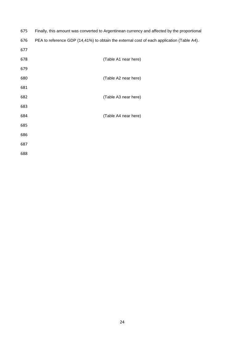
Finally, this amount was converted to Argentinean currency and affected by the proportional 675

PEA to reference GDP (14,41%) to obtain the external cost of each application (Table A4). 676

677

(Table A1 near here) 678

679


681


683


685

686

687

688

25

Table 1. Model Based Weed Management DSSs 689

690

Reference/ Denomination

Weed/Crop Country of

development

Model components Evaluation approach Scope Environmental

Impact4 Climatic

1

Biological2

Economic Simulation Optimization3 Operational Tactical/Strategic

Empirical Mechanistic

Doyle et al. (1986) Cousens et al. (1986)

Alopecurus myosuroides, Avena fatua/ Winter wheat

United Kingdom X X X X

Sells (1995) Avena fatua, Alopecurus myosuroides

United Kingdom X X X X

Wiles et al. (1996)/ GWM

General USA X X X X

Berti et al. (1997), Berti et al. (2003)/ GESTINF

16 weed species/ Soybean, wheat

Italy X X X X

De Buck et al. (1999)/ BESTWINS

4 weed species/ Sugar beet

The Netherlands

X X X X X

Falconer and Hodge (2001)

General United Kingdom

X X X X X

Mullen et al. (2003) Striga sp. Mali X X X

González- Andújar and Fernández- Quintanilla (1991, 2004)

Avena sterilis, Lolium rigidum

Spain X X X

Pannell et al. (2004) / RIM

Lolium rigidum Australia X X X X

Rydahl (2004)/ CPO 75 weed species/ 11 crops

Denmark X X X

Colbach et al. (2007)/ ALOMYSYS

Alopecurus myosuroides

France X X X X X

Parsons et al. (2009)/ Weed Manager

13 weed species/ Winter wheat

United Kingdom

X X X X X X

Torra et al. (2010)/ PIM

Papaver rhoeas Spain X X X X

This paper Avena fatua / Winter wheat

Argentina X X X X X

1: Considered in a quantitative fashion (degree days, etc.) 2: Considers items such as: seed survival, dormancy, germination, pre-emergence growth, seedling survival, tillering, heading, flowering , seed production 3: Implements a numerical optimization algorithm to perform the search 4: Considered in a quantitative fashion

26

Table 2. Model indexes and variables 691

692

Indexes

Symbol Name

t Time period (calendar days)

h hs, hns Herbicide (s: selective, ns: non-selective)

Variables

Symbol Name

Dt Weed density (plants m-2)

TDEt Daily time-density equivalent (plants m-2)

TDEtot Global TDE (plants m-2)

Ettt Weed plants emerged at day t that survive and affect crop yield (plants m-2)

EMtt,h Weed plants emerged at day t killed by application of herbicide h (plants m-2

)

bight,h Total applications of herbicide h during a period of (nsh2h – nsh1h) days

Mt Daily weed seedling mortality (plants m-2)

Mtht,h Daily weed seedling mortality due to herbicide h (plants m-2)

yL Crop yield loss (%)

y Crop yield (kg ha-1)

B Economic benefit ($ ha-1)

Inc Gross income ($ ha-1)

Cost Cost of herbicide applications ($ ha-1)

Ext Environmental cost of herbicide applications ($ ha-1)

yhthh,t Binary variable; 1 if herbicide h is applied; 0 instead

693

694

695

27

Table 3. Weed and crop parameters 696

697

Symbol Name Parameter value

Et Daily weed emergence (plants m-2

day-1) Section 3

a Parameter of equation (1) 100

i Parameter of equation (1) 0.75

c Parameter of equation (4) 0.119

Temt Day of weed emergence (days) Section 2.3

ywf Weed-free crop yield (kg ha-1) 2000

pc Crop price ($ kg-1) 0.75

ns Period of crop susceptibility to herbicides (days) 26

Tec Period of time from sowing to crop emergence (days) 17

Dec Day of crop emergence (days) Section 2.3

Des Day of crop sowing (days) 152

RTt Relative time of crop-weed emergence (days) Section 2.3

bigM Big M constant 50000

nsh1h Day of beginning of weed susceptibility to herbicide (days) Table 4

nsh2 h Day of end of weed susceptibility to herbicide (days) Table 4

PEAh External cost of one application of herbicide h ($ ha-1) Table 4

costhh Cost of herbicide ($ ha-1) Table 4

698

699

700

701

702

703

704

705

706

707

708

709

710

711

712

713

714

28

Table 4. Herbicides parameters 715

716

Type Cost ($ ha-1) nsh1 (day) nsh2 (day) PEA ($ ha

-1)

Pinoxaden selective 141.88 10 36 0.15

Clodinafop selective 161.53 10 36 0.16

Fenoxaprop selective 300.14 10 36 0.27

Pyroxsulam selective 114.60 10 36 0.21

Diclofop - methyl selective 158.26 10 27 2.40

Tralkoxydim selective 111.65 10 27 0.65

Glyphosate non-selective 31.11 1 36 1.94

Paraquat non-selective 53.48 1 36 2.08

717

718

719

720

721

722

723

724

725

726

727

728

729

730

731

732

733

734

735

736

737

738

739

29

Table 5. Results summary 740

741

Case 1 (2003) Case 2 (2004) Case 3 (2007)

Final weed density (plants m-2) 61 154 72

TDEtot (plants m-2) 18 3 23

Crop yield loss (%) 11.9 2.4 14.8

Crop yield (kg ha-1) 1761.8 1952.6 1703.9

Income ($ ha-1) 1321.4 1464.4 1277.9

Cost ($ ha-1) 207.9 62.2 93.3

Externalities ($ ha-1) 6.0 3.9 5.8

Benefit ($ ha-1) 1107.4 1398.3 1178.8

Selected herbicide type: Application days

Glyphosate: 77/114/150 Pyroxsulam: 196

Glyphosate: 110/147

Glyphosate: 79/115/151

742

743

744

745

746

747

748

749

750

751

752

753

754

755

756

757

758

759

760

761

762

30

Table 6. Sensitivity analysis (seed bank) 763

764

Variable Percentage of change

-25% -20% -10% Base Case +10% +20% +25%

Seed bank (seeds m

-2)

150 160 180 200 220 240 250

Final weed density (plants m

-2)

45 66 54 61 66 72 76

TDEtot (plants m-2) 9.3 23.4 14.7 18.0 17.9 17.4 25.0

Crop yield loss (%) 6.5 14.9 9.9 11.9 11.9 11.5 15.8

Crop yield (kg ha-1) 1869.7 1701.7 1801.9 1761.8 1762.2 1769. 2 1684.1

Income ($ ha-1) 1402.3 1276.3 1351.4 1321.4 1321.6 1326. 9 1263.1

Cost ($ ha-1) 207.9 93.3 207.9 207.9 207.9 207.9 207.9

Externalities ($ ha-1) 6.0 5.8 6.0 6.0 6.0 6.0 6.0

Benefit ($ ha-1) 1188.3 1177.1 1137.4 1107.4 1107.7 1112.9 1049.1

Selected herbicide type: Application periods








765

766

767

768

769

770

771

772

773

774

775

776

777

778

31

Table 7. Sensitivity analysis (weed susceptibility period) 779

780

Variable Percentage of change

-10% Base case 10%

Final weed density (plants m-2) 83 61 58

TDEtot (plants m-2) 33.0 18.0 6.3

Crop yield loss (%) 19.8 11.9 4.5

Crop yield (kg ha-1) 1603.1 1761.8 1909.2

Income ($ ha-1) 1202.3 1321.4 1431.9

Cost ($ ha-1) 93.3 207.9 207.9

Externalities ($ ha-1) 5.8 6.0 6.0

Benefit ($ ha-1) 1103.1 1107.4 1217.9

Selected herbicide type: Application periods




781

782

783

784

785

786

787

788

789

790

791

792

793

794

795

796

797

798

799

800

32

Table A1. EIQ Calculation 801

802

Active ingredient Pinoxaden Clodinafop Fenoxaprop Pyroxsulam Diclofop

methyl Tralkoxydim Glyphosate Paraquat

Cloquintocet

mexyl

Metsulfuron

methyl

EIQ per category

Applicator effects 5 15 5 5 15 15 5 15 5 5

Picker effects 3 9 3 3 9 9 3 9 3 3

Consumer effects 2 6 2 2 6 6 3 4 2 4

Ground water 3 1 1 1 1 1 1 1 1 3

Aquatic effects 3 25 25 3 9 15 3 1 1 3

Bird effects 6 6 6 6 6 6 9 12 6 12

Bee effects 9 9 9 9 9 9 9 9 9 9

Beneficial insects effects 15 15 15 15 45 15 15 45 15 15

EIQ 15.33 28.67 22 14.67 33.33 25.33 16 32 14 18

% a.i. in formulation 5 8 6.9 4.5 28.4 80 36a 27.6 1.25

b – 2

c –

9d

60

Rate (Kg or l formulation

per ha)

0.6 0.36 0.85 0.4 2 0.2 1.5 2 0.60b – 0.36

c

– 0.40d

0.0067

EIQ field use rating 0.46 0.83 1.29 0.26 18.93 4.05 8.64 17.66 0.11b – 0.10

c

– 0.50d

0.07

aacid equivalent concentration in formulation

b in pinoxaden formulation

c in clodinafop formulation

d in pyroxsulam formulation

33

Table A2. EIQ Variables 803

804

Symbol Name

DT Dermal toxicity

C Chronic toxicity

P Plant surface residue half-life

S Soil residue half-life

SY Pesticide mode of action

L Leaching potential

F Fish toxicity

R Surface loss potential

D Bird toxicity

Z Bee toxicity

B Beneficial arthropod toxicity

805

806

807

808

809

810

811

812

813

814

815

816

817

818

819

820

821

822

823

824

825

34

Table A3. Quotient classification for each EIQ category 826

827

EIQ categories Low range (0.5) Medium range (1) High range (1.5)

Applicator effects 5 ≤ EIQ < 25 25 ≤ EIQ < 85 85 ≤ EIQ ≤ 125

Picker effects 1 ≤ EIQ < 14 14 ≤ EIQ < 76 76 ≤ EIQ ≤ 125

Consumer effects 1 ≤ EIQ < 14 14 ≤ EIQ < 76 76 ≤ EIQ ≤ 125

Ground water 1 ≤ EIQ < 2 2 ≤ EIQ < 4 4 ≤ EIQ ≤ 5

Aquatic effects 1 ≤ EIQ < 5 5 ≤ EIQ < 17 17 ≤ EIQ ≤ 25

Bird effects 3 ≤ EIQ < 15 15 ≤ EIQ < 51 51 ≤ EIQ ≤ 75

Bee effects 3 ≤ EIQ < 15 15 ≤ EIQ < 51 51 ≤ EIQ ≤ 75

Beneficial Insects effects 5 ≤ EIQ < 25 25 ≤ EIQ < 85 85 ≤ EIQ ≤ 125

The numbers between brackets are the weights applied to each range

828

829

830

831

832

833

834

835

836

837

838

839

840

841

842

843

844

845

846

847

848

849

35

Table A4. Estimated field use external costs of eight herbicides included in the model 850

851

Active ingredient

Pinoxaden +

Cloquintocet

mexyl

Clodinafop +

Cloquintocet

mexyl

Fenoxaprop

Pyroxsulam +

Cloquintocet

mexyl +

Metsulfuron

methyl

Diclofop methyl Tralkoxydim Glyphosate Paraquat

Per hectare cost

($ARS)

Applicator effect 0.01 0.01 0.02 0.02 0.20 0.06 0.19 0.20

Picker effect 0.01 0.01 0.02 0.02 0.14 0.04 0.14 0.14

Consumer effect 0.06 0.06 0.09 0.10 0.94 0.27 0.90 0.92

Ground water 0.03 0.01 0.02 0.03 0.23 0.06 0.22 0.22

Aquatic effects 0.02 0.04 0.08 0.03 0.52 0.15 0.25 0.25

Birds effects 0.01 0.01 0.01 0.01 0.10 0.03 0.09 0.10

Bee effects 0.01 0.01 0.01 0.01 0.07 0.02 0.07 0.07

Beneficial insects

effect 0.01 0.01 0.01 0.01 0.2 0.03 0.09 0.19

Total ($ARS) 0.15 0.16 0.26 0.23 2.4 0.66 1.95 2.09

36

852

Fig. 1. Avena fatua emergence patterns analyzed using the operational model

Fig. 2. Case 1: Evolution of total weed density (D(t), plants m-2

) (solid line) and weed density

affecting crop yield (TDEtot, plants m-2

) (dashed line). Arrows indicate the time of herbicide

applications.

Fig. 3. Case 2: evolution of total weed density(D(t), plants m-2




applications.

Fig. 4. Case 3: evolution of total weed density (D(t), plants m-2




applications.

Figure captions

0 100 200 3000

50

1002003

2004

2007

t (calendar days)

Accum

ula

ted e

me

rge

nce (

%)

Fig. 1. Avena fatua emergence patterns analyzed using the operational model

Figure 1

0 100 200 3000

10

20

30

40

50

60

70D(t)

TDEtot

t (calendar days)

Pla

nts

/m2

Fig. 2. Case 1: Evolution of total weed density (D (t), plants m-2




applications.

Figure 2

0 100 200 3000

20

40

60

80

100

120

140 D(t)

TDEtot

t (calendar days)

Pla

nts

/m2

Fig. 3. Case 2: evolution of total weed density (D (t), plants m-2




applications.

Figure 3

0 100 200 300 4000

10

20

30

40

50

60

70

80

90D(t)

TDEtot

t (calendar days)

Pla

nts

/m2

Fig. 4. Case 3: evolution of total weed density (D (t), plants m-2




applications.

Figure 4

Operational planning of herbicide-based weed management

Documents

Transcript of Operational planning of herbicide-based weed management