Operational Modal Analysis in presence of dynamic interaction among adjacent buildings-an assessment

Operational Modal Analysis in presence of dynamic interaction among adjacent buildings - an assessment

C. Rainieri1, G. Fabbrocino

1, G. Manfredi

2, M. Dolce

3

1 University of Molise, Structural and Geotechnical Dynamics Lab, Department SAVA

Via Duca degli Abruzzi, 86039, Termoli, Italy

email: [email protected], [email protected]

2 University of Naples Federico II, Department of Structural Engineering

Via Claudio 21, 80125, Napoli, Italy

email: [email protected]

3 Department of Italian Civil Protection, Seismic Risk Office

Via Vitorchiano 4, 00189,Roma, Italy

email: [email protected]

Abstract Operational Modal Analysis relies upon the fundamental assumption that input is unmeasured and consists

of a Gaussian white noise characterized by a flat spectrum in the bandwidth of interest. If this assumption

is not fulfilled, the modal identification process may fail due to spurious frequencies appearing in response

spectra. It is often possible to identify such non-structural frequencies, but they can also sometimes bias

estimates. This is basically the case of spurious harmonics close to structural modes. About civil

structures, spurious frequencies can be due to rotating machines but also to interaction with adjacent

constructions, as discussed herein, where natural frequencies of a given structure are mixed together with

those ones due to interaction with similar close structures; as a result, response spectra are characterized

by several close peaks in a narrow bandwidth. An integrated use of output-only techniques is proposed to

discriminate modal from spurious frequencies and applied to a real test case.

1 Introduction

A fundamental assumption of Operational Modal Analysis (OMA) is that input, being it not measured,

consists of a Gaussian white noise with a flat spectrum in the frequency range of interest. As a

consequence, all modes are assumed to be equally excited in this range and they can be extracted by

appropriate methods. However, if this assumption is not fulfilled, the modal parameter identification

process may fail since frequencies not corresponding to actual modes appear in response spectra.

The assumption about the stochastic nature of input forces in OMA is usually fulfilled in the case of civil

engineering structures. Buildings, bridges, towers, in fact, are mainly excited by wind, traffic or seismic

micro-tremors. The problem of combination of a stochastic broadband input with harmonic components,

deterministic in nature, is more relevant in the case of mechanical structures, such as in-flight helicopters,

running engines [1] and ships in operation [2]. Nevertheless, also civil engineering structures can show

harmonic components superimposed to the stochastic response. They can be due, for example, to turbines,

generators, ventilation systems and other mechanical components and systems installed in the buildings or

in adjacent areas.

Some approaches to solve the problem of discriminating harmonic components from actual structural

modes in OMA are available in technical literature. This issue is extensively analyzed in [3], where

popular OMA methods are reviewed (Polyreference Least Square Complex Exponential [4], Ibrahim Time

743

Domain [5] and Eigensystem Realization Algorithm [6]) and modified in order to manage effects of

harmonic excitations. Influence of harmonic components on OMA carried out according to the (Enhanced)

Frequency Domain Decomposition procedure [7, 8] and the Stochastic Subspace Identification methods

[9, 10] is investigated and summarized in [11], where also a number of methods able to discriminate

harmonic components from structural modes is reported.

From a general point of view, the main drawbacks concerning the presence of deterministic signals

superimposed to the stochastic part can be summarized as follows:

Potential mistakes in identification of modes, that is to say harmonics can be erroneously

identified as structural modes;

Potential bias in mode estimation, affecting natural frequency, damping and/or mode shape, in

particular if the spurious harmonic is very close to the structural mode;

Need of a high dynamic range to extract weak modes in presence of such harmonics.

Different criteria are available to identify harmonic components. In [12] it is observed that harmonics in

response spectra can be identified as narrowband resonances whose bandwidth depends on frequency

resolution. Thus, if the bandwidth changes with frequency resolution, the resonance is likely a spurious

harmonic. Alternative strategies rely upon: 1) examination of Short Time Fourier Transform of response

signals, 2) rank estimation of the output Power Spectral Density matrix at the frequency of interest via

Singular Value Decomposition, 3) elimination of frequencies associated to unlikely modal properties

(unrealistic mode shapes, too much low damping ratios) [2, 11, 13]. More advanced strategies to identify

and remove spurious harmonics are based on checks of Probability Density Functions and, in particular, of

kurtosis [14, 15].

In the present paper, the issue of identification through OMA of structural modes in presence of spurious

dominating frequencies is addressed. It starts from the experimental campaign carried out under the

coordination of the Italian Civil Protection in the area of the Guardia di Finanza Non-Commissioned

Officers’ School in Coppito, L’Aquila, Italy.

In particular, an extensive dynamic characterization of the buildings has been carried out to support

inspections and provide information to the Civil Protection during post-mainshock emergency

management of buildings and implementation of permanent monitoring systems. The description of such a

complex activity is out of the scope of the present work, but the relevant number of performed dynamic

tests under environmental excitation provided interesting sample cases.

Among them, measures taken on four buildings in Block B1 located in the area of the Guardia di Finanza

School are analyzed in the following. Actually, the test case relevance cannot be addressed to as much

narrowband excitation due to rotating parts as to interaction effects with other close structures

characterized by similar natural frequencies. As a consequence, response spectra show several peaks in a

narrow frequency range and just a few of them are related to structural modes; the others are, conversely,

correlated to interaction effects among the close structures.

In the following sections, after a short description of constructions and of test layout, the problem of

modal identification in presence of dynamic interaction effects is analyzed and results provided by

different OMA methods are discussed.

2 Description of the construction and test layout

2.1 Block B1 overview

Block of buildings B1 is located in the area of the Guardia di Finanza Non-Commissioned Officers’

School in Coppito. It consists of nine similar reinforced concrete moment frame buildings distributed on

three lines and covers a rectangular area of 165 m by 66 m. At time of testing, they were used as residence

for cadets. Connection among the different buildings and vertical distribution are ensured by a number of

separated reinforced concrete stairs. Indoor stairs are located in the intermediate courtyards, outdoor stairs

744 PROCEEDINGS OF ISMA2010 INCLUDING USD2010

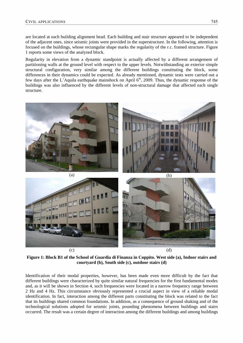
are located at each building alignment head. Each building and stair structure appeared to be independent

of the adjacent ones, since seismic joints were provided in the superstructure. In the following, attention is

focused on the buildings, whose rectangular shape marks the regularity of the r.c. framed structure. Figure

1 reports some views of the analyzed block.

Regularity in elevation from a dynamic standpoint is actually affected by a different arrangement of

partitioning walls at the ground level with respect to the upper levels. Notwithstanding an exterior simple

structural configuration, very similar among the different buildings constituting the block, some

differences in their dynamics could be expected. As already mentioned, dynamic tests were carried out a

few days after the L’Aquila earthquake mainshock on April 6th, 2009. Thus, the dynamic response of the

buildings was also influenced by the different levels of non-structural damage that affected each single

structure.

(a)

(b)

(c)

(d)

Figure 1: Block B1 of the School of Guardia di Finanza in Coppito. West side (a), Indoor stairs and

courtyard (b), South side (c), outdoor stairs (d)

Identification of their modal properties, however, has been made even more difficult by the fact that

different buildings were characterized by quite similar natural frequencies for the first fundamental modes

and, as it will be shown in Section 4, such frequencies were located in a narrow frequency range between

2 Hz and 4 Hz. This circumstance obviously represented a crucial aspect in view of a reliable modal

identification. In fact, interaction among the different parts constituting the block was related to the fact

that its buildings shared common foundations. In addition, as a consequence of ground shaking and of the

technological solutions adopted for seismic joints, pounding phenomena between buildings and stairs

occurred. The result was a certain degree of interaction among the different buildings and among buildings

CIVIL APPLICATIONS 745

and stairs (both interior and exterior) so that natural frequencies of a certain building or stair appeared in

the dynamic response in operational conditions of other close buildings in the block. A plane view of the

block is reported in Figure 2. In the same picture, tested buildings are identified by number 2, 3, 5 and 6,

whose relevant dimensions are 48,7 m by 15,40 m.

Figure 2: Plane view of tested building: nine buildings jointed among them and with stairs

2.2 Test setup

As already mentioned, measurements of the dynamic response of the structure have been carried out a few

days after the last L’Aquila earthquake in order to monitor its dynamic behavior and its health state during

aftershocks, as a support to visual inspections for structural damage detection, refined numerical analyses

for capacity assessment and eventual installation and operation of a structural health monitoring system.

Thus, measurement setup was designed in order to cover the highest number of buildings at the same time.

A moderate number of sensors has been therefore installed on each tested building, in a way able to ensure

identification of at least the fundamental modes in compliance with current seismic design guidelines.

A tern of sensors in three orthogonal directions has been also installed on the basement in order to

eventually measure input at the base of the structure due to ground motion. Even if the whole

measurement setup is described here, just records of the dynamic response of the structure in operational

conditions due to ambient vibrations are taken into account for data processing in Section 4.

Sensor layout for the four monitored buildings is reported in Figure 3. Buildings n. 2 and 3 have been

monitored at the upper level and at the intermediate level. Four sensors have been installed in two opposite

corners at each level in two orthogonal directions in order to ensure observability of both translational and

torsional modes. Buildings n. 5 and 6, instead, have been monitored by only two couples of sensors placed

according to two orthogonal directions parallel to the main axes of each building at the upper level.

However, in the data processing phase it has been recognized that sensor n. 3 in x direction on building n.

5 was out of order and it has not been used in the modal identification process. Thus, just three sensors

were available for dynamic characterization of building n. 5 and its proper modal identification has been

affected and made even more difficult by this circumstance.

Dynamic responses of buildings n. 2 and 3 have been measured by means of uniaxial force balance

accelerometers (Kinemetrics Episensors ES-U2), while piezoelectric accelerometers (PCB Piezotronics

model 393B31) have been installed on buildings n. 5 and 6. Characteristics of the installed sensors are


summarized in Table 1. They have been selected in order to ensure high quality measurements in

operational conditions but also the possibility to properly measure the structural response to expected

ground motions. The tern of sensors installed on the common basement of the building was made by three

Kinemetrics Episensors ES-U2 mounted according to three orthogonal directions in order to measure also

eventual vertical components of ground motion.

72nd floor

8

5

6

x

y1

3rd floor

2

34

(a)

52nd floor

6

7

8

x

y

3

4

3rd floor

21

(b)

3rd floor

21

x

y 3

4

(c)

3rd floor

43

x

y 1

2

(d)

Figure 3: Sensor layout for building n. 2 (a), 3 (b), 5 (c) and 6 (d)

Sensor Measurement

directions Sensitivity

[V/g]

FS range

[g]

Reso-lution [g rms]

Dynamic range [dB]

Bandwidth [Hz]

Transverse sensitivity

Non-linearity

Episensor ES-U2

1 20 0.5 - 140 0-200 ≤1% <1000 µg/g2

393B31 1 10.0 0.5 0.000001 - 0.1-200 ≤5% ≤1%

Table 1: Sensor characteristics

Recorder Measurement

channels Resolution

[bit]

Sampling frequency

[Hz]

Input coupling [g rms]

Cross-talk [dB]

CMMR [dB]

TrioGuard 32 32 16 Up to

250000 DC -90 92

Table 2: Data acquisition hardware characteristics

Vibration data have been acquired through a TrioGuard32 data acquisition recorder. It is a versatile

multifunction recorder able to acquire dynamic data from a number of different sensors including force

balance and piezoelectric accelerometers. Its characteristics are summarized in Table 2.

Sensors have been installed on steel plates screwed on the floor. Cable have been clamped to the structure

along the whole path to the data acquisition recorder in order to avoid introduction of measurement noise

by triboelectric effects due to cable motion. Careful attention has been paid to avoid as much as possible


all noise sources (including those ones due to the magnetic field induced by mobile phones and other

communication devices close to the measurement chain).

Tests have been carried out by simultaneously acquiring data, at a sampling frequency equal to 100 Hz,

from the 27 accelerometers installed over the block of buildings. Each record was 3600 sec long. The

dynamic response of the buildings has been continuously monitored for more than two consecutive days,

thus leading to more than 50 records, some of which including the structural response to ground motions.

As already mentioned, in the context of the present study, only records of the structural response to

ambient vibrations are considered.

Before processing, records have been accurately inspected in order to assess their quality. Offsets and

spurious trends in data have been removed. Data have been also decimated in order to have a final

sampling rate equal to 20 Hz. During data processing in frequency domain, spectra have been computed

by assuming a 66% overlap and using a Hanning window.

3 Modal identification procedures

Output-only modal parameter estimation has been carried out according to the Covariance Driven

Stochastic Subspace Identification (Cov-SSI) [10], the Enhanced Frequency Domain Decomposition

(EFDD) [7, 8] and the Second Order Blind Identification (SOBI) [16]. Moreover, an automated output-

only modal identification procedure, LEONIDA [17], has been also applied to the present case study. The

present section briefly reports the basics of the above mentioned reference methods.

The (Enhanced) Frequency Domain Decomposition technique is based on the Singular Value

Decomposition (SVD) of the output Power Spectral Density (PSD) matrix, which has been previously

estimated directly from the raw data at discrete frequencies ω=ωi:

Hiiiiyy USUjG

(1)

where the matrix [U]i is a unitary matrix holding the singular vector uij and [S]i is a diagonal matrix

holding the scalar singular values sij. Near a peak corresponding to the kth mode in the spectrum, this mode

will be dominant. If only the kth

mode is dominant, there will be one term in Equation (1) and the PSD

matrix approximates to a rank one matrix as:

ki

H

iiiiyy uusjG

11 (2)

In such case, the first singular vector 1iu is an estimate of the mode shape:

1ˆ

iu (3)

and the corresponding singular value belongs to the Auto Power Spectral Density function of the

corresponding Single Degree Of Freedom (SDOF) system. In case of repeated modes, the PSD matrix

rank is equal to the number of multiplicity of the modes. The Auto Power Spectral Density function of the

corresponding SDOF system is identified around the peak of the singular value plot by comparing the

mode shape estimate ̂ with the singular vectors associated to the frequency lines around the peak.

Every line characterized by a singular vector which gives a MAC value [18] with ̂ higher than a user-

defined MAC Rejection Level belongs to the SDOF PSD function. This equivalent SDOF PSD function is

used, according to the EFDD algorithm, for natural frequency and damping estimations. The former are

independent upon the frequency resolution of the spectra computed by the Fast Fourier Transform (FFT)

algorithm. In fact, the SDOF PSD function is transferred back to time domain through Inverse FFT, so that

an approximated correlation function of the equivalent SDOF system is obtained. Then a linear regression

on the zero crossing times of such correlation function is carried out in order to extract the natural

frequency, by properly taking into account the relation between damped and undamped natural frequency.


The damping ratio is also computed starting from the free decay function of the SDOF system by the

logarithmic decrement technique.

Stochastic Subspace Identification (SSI) methods work in time domain and are based on a state space

description of the dynamic problem [9, 10]. In fact, the second order problem, stated by the differential

equation of motion, is converted into two first order problems, defined by the so-called “state equation”

and “observation equation”. Such equations, in the output-only case, can be written as follows:

kkk wxAx 1 ; kkk vxCy (4)

where tkxxk is the discrete-time state vector yielding the sampled displacements and velocities,

ku and ky are the sampled input and output, A is the discrete state matrix, C is the discrete

output matrix, kw is the “process noise” due to disturbances and model inaccuracies, kv is the

“measurement noise” due to sensor inaccuracy. These vector signals are both unmeasurable: they are

assumed to be zero mean Gaussian white noise processes with covariance matrices given by:

pqT

T

q

T

q

p

p

RS

SQvw

v

wE

(5)

where E is the expected value operator, pq is the Kronecker delta (if p=q then 1pq , otherwise

0pq ), p and q are two arbitrary time instants. In the stochastic framework which characterizes OMA,

due to the lack of information about the input, it is implicitly modeled by the noise terms kw and kv .

The white noise assumption about kw and kv cannot be omitted for the proof of this class of

identification methods (see also [9]). If this assumption is violated, that is to say the input includes white

noise and some additional dominant frequency components, such components will appear as poles of the

state matrix [A] and cannot be separated from the eigenfrequencies of the system. Covariance Driven

(Cov-SSI) and Data Driven (DD-SSI) SSI are two algorithms for estimation of system matrices and,

therefore, of eigenproperties. The main difference is related to the fact that Cov-SSI works on output

correlations while DD-SSI works directly on raw data.

SOBI is a Blind Source Separation (BSS) technique for signal processing and data analysis that, given a

series of observed signals, aims at recovering the underlying sources. In [16] it is shown that, under given

assumptions, modal coordinates act as virtual sources, thus allowing application of such methodology for

modal parameter identification in output-only conditions. BSS techniques can be addressed as non-

parametric procedures for modal identification since the mixing model is the only assumption.

The SOBI algorithm finds components that approximately produce diagonal time-shifted covariance

matrices. The main steps of the algorithm can be summarized as follows:

observed data [x(t)] are centralized, removing the mean value from each component of [x(t)], and

whitened (basically through a Principal Component Analysis);

whitened data are used to build a number of time shifted covariance matrices;

a numerical algorithm based on the Jacobi rotation technique [19] is then used to recover the

mixing matrix;

mode shapes are extracted directly from the mixing matrix [A], while natural frequencies and

damping ratios are obtained through a Single Degree Of Freedom (SDOF) curve fitting of the

sources.

LEONIDA is an FDD-based algorithm for automated output-only modal identification. It is based on the

repeated computation of the SVD of the PSD matrix for a number of records and on inspection of the

sequence of MAC values computed, at each frequency line, between singular vectors obtained from two

records. An averaged MAC vs. frequency plot is also obtained. It looks like a coherence function.

Inspecting the sequence of MAC values at each frequency line it is possible to identify the actual mode

bandwidth to be used for modal parameter extraction. Currently, the algorithm refers to some limit values


affecting MAC and its first derivative. They produce identification of the frequency lines belonging to a

certain mode bandwidth. Such limits are the results of a calibration process based on records obtained

from different measurement setups, with different durations and related to different kinds of structures

[17]. Thus, an objective identification of mode bandwidth is possible.

4 Output-only modal identification and interaction effects

Starting from records of the dynamic response of the four monitored buildings due to ambient vibrations,

an output-only modal identification process has been carried out according to the previously outlined

methodologies. As already mentioned, complexity of the present case study was basically related to

dynamic interaction effects among close buildings and stairs. As a result, response spectra show several

peaks in a narrow frequency range between 2 and 4 Hz. In order to visualize it, Singular Value (SV) plots

provided by SVD of the output PSD matrix in the framework of the FDD procedure are reported in Figure

4. Complexity is increased also by the aspect of peaks due to dynamic interaction, which do not appear as

sharp-pointed resonances, such as in the case of spurious harmonics induced by rotating parts.

(a)

(b)

(c)

(d)

Figure 4: SV plots for building n. 2 (a), 3 (b), 5 (c), 6 (d)

Output-only modal identification has been therefore carried out with reference to each of the methods

described in the previous section. First stage results have been collected, compared and analyzed

according to a number of criteria. Thus, first of all a traditional identification process has been carried out.

In all cases it has been mainly based on user experience. The only exception is represented by data

processing carried out by LEONIDA, which is a fully automated OMA procedure and, as such, it does not

require any user intervention. User knowledge and best practice rules have been used first of all to identify

all peaks in the SV plots which could be probably related to structural modes. When Cov-SSI has been


applied to output-only modal identification, instead, user played a relevant role for selection of stable

poles which could most likely represent structural modes. Finally, when SOBI has been applied, sources

probably related to structural modes have been carefully considered and selected according to the specific

method best practice.

Method

Frequency [Hz] EFDD Cov-SSI SOBI LEONIDA

2.18 x - - -

2.54 x x x

(not separated from 5.28) -

2.64 - x - -

2.85 x x X x

2.98 - x - -

3.49 x x X x

5.28 x x x

(not separated from 2.54) x

7.05 x x - x

Table 3: Results of first stage modal identification (building n. 2)

Method


2.18 x - - -

2.54 x x x x

2.86 x x not well separated x

2.99 x - - -

3.19 x - - -

3.48 x x x x

5.26 x - x -


Method


2.20 x x x

(not well separated) -

2.41 x x - -

2.66 x x x x

3.16 x x - x

3.93 x x x x


After this preliminary phase, a number of candidates as structural modes have been identified for each


building. The corresponding natural frequencies are summarized in Table 3, Table 4, Table 5 and Table 6,

where crosses point out methods considering such frequency as a potential natural frequency. Selection of

structural modes has been then carried out by inspecting a number of characteristics of the candidates. In

particular, coherence among couples of channels, complexity of mode shapes, aspect of mode shape,

damping ratio value, number of methods identifying a certain mode as a structural one have been

considered as selection criteria.

Method


2.20 x x x


2.41 x x - -

2.65 x x x


2.81 x x x


3.20 x x - -

3.47 x x - -

3.93 x x x x

5.78 x x x


7.50 x x - x


However, they have been considered just in a positive sense, that is to say they have been considered as

indications of possible presence of a structural mode more than as evidence that a potential candidate is a

spurious pole. Then, only poles fulfilling all or nearly all criteria have been selected as structural modes.

This choice is justified, for example, by the fact that, being the number of sensors on some buildings very

limited (three working sensors on building n. 5) and being the number of identifiable modes lower or

equal than the number of sensors when SOBI is applied to output-only modal identification, it is likely that

some modes are missing among SOBI results but they are identified by all other methods. According to

the above mentioned criteria and comparing candidates of the different buildings, it was possible to

identify a number of modes which can be reliably considered as structural modes. The logical process and

some additional details are summarized in Table 7.

It is worth pointing out how, in the present case study, reasonable damping values were associated to

candidate modes, so their inspection has been not useful to discriminate structural modes. Also complexity

of mode shape and coherence have sometimes given inconsistent indications. In fact, modes identified as

structural by all methods can show some little imaginary components in their shapes which could be

probably due to some noise effects; conversely, real shapes can be associated to spurious frequencies.

Moreover, high values of coherence between couples of channels are not always sign of the presence of a

structural mode. Thus, potential candidates have been classified as structural modes if they complied with

most of the adopted criteria and were identified by almost all methods.

The above described inspections and comparisons allowed a reliable identification of the modes

summarized in Table 8 as structural modes of the monitored buildings. It is possible to note that the

sequence of modes is not the same among the different buildings notwithstanding their apparently similar

geometry. This circumstance can be justified in different ways. It is possible that the first mode in x

direction is missing for building n. 2 and n. 5, being the selection criteria arbitrarily defined.

Actually, observing that LEONIDA was able to identify all modes that have been then selected as


structural modes, neglecting all other candidates and with just a false positive (at 2.65 Hz for building n.

6), and that identification results provided by LEONIDA are quite stable over different records (Table 9),

it is possible that this assumption fails, unless the first mode is always very weakly excited so that

LEONIDA is not able to identify it according to its preset parameters.

Building n. 2 Building n. 3 Building n. 5 Building n. 6

Frequency (Hz) 2.18 2.18 2.20 2.20

Remarks

Pure x transl. (EFDD);

coherence 0.93 –

Interaction building n. 3

Complex mode –

Interaction building n. 5

Complex mode –

interaction building n. 6

Pure x transl.

Frequency (Hz) 2.54 2.54 2.41 2.41

Remarks

Pure x transl.;

coherence 0.99 –


Pure x transl. Interaction or x transl.

(few sensor to say)

x transl.; coherence

0.93; Interaction with unmeasured structure

Frequency (Hz) 2.64 2.86 2.66 2.65

Remarks Complex mode;

interaction buildings n.

5 and 6

Mainly y transl.; not

fully stable (SSI);

coherence 0.99

Mainly y transl. y transl.; interaction

building n. 5

Frequency (Hz) 2.85 2.99 3.16 2.81

Remarks Mainly y transl.

Mainly y transl.;

coherence 0.93;

interaction with unmeasured structure

Mainly y transl.; slightly complex

Mainly y transl.

Frequency (Hz) 2.98 3.19 3.93 3.20

Remarks Complex mode;


Complex mode;


Torsion Complex mode;


Frequency (Hz) 3.49 3.48 3.47

Remarks Torsion Torsion Complex mode;


Frequency (Hz) 5.28 5.26 3.93

Remarks Mainly x transl.

Unstable poles (SSI);

real mode; unlikely

mode shape;


Torsion

Frequency (Hz) 7.05 5.78

Remarks Torsion Pure x transl.

Frequency (Hz) 7.50

Remarks Torsion

Table 7: Summary of preliminary analysis

Another possible motivation is related to the pounding phenomena among close buildings and stairs and to

damage of partition walls caused by the mainshock of L’Aquila earthquake at a major extent for those

buildings, which could have had an effect on the original structural modes. It is less probable, instead, that

some modes are missing due to observability issues. In fact, even if the number of sensors was quite


limited, they should be enough in number and properly displaced so that observability of at least

fundamental modes is assured. This is not strictly true only for building n. 5 due to the fact that one of the

installed sensors revealed itself to be out of order.

Nevertheless, it is worth noting how the proposed approach, based on combination of results provided by

different OMA methods and on a number of selection criteria, has been able to reliably identify the

fundamental modes of the four monitored buildings of the structure under test, discriminating them from

frequencies related to dynamic interaction effects and transmitted among the different buildings so that the

input spectrum on each one of them is not strictly flat as assumed by OMA methods.

Finally, it is interesting to note how the buildings were excited also by a spurious harmonic at 6.2 Hz

which was due to some equipments (probably, a plumbing) located in the basement of the building. Such

harmonic can be clearly identified in Figure 4 as a sharp-pointed resonance. Moreover, it is important to

note that it is far enough from relevant structural modes so that their identification is not biased by its

presence.


Modal Frequency (Hz)

Remarks

2.85

Mainly y transl.

2.54

Pure x transl.

2.66

Mainly y transl.

2.20

Pure x transl.


Remarks

3.49

Torsion

2.86

Mainly y transl.

3.16

Mainly y transl.

2.81

Mainly y transl.


Remarks

5.28

Mainly x transl.

3.48

Torsion

3.93

Torsion

3.93

Torsion


Remarks

7.05

Torsion

5.78

Pure x transl.


Remarks

7.50

Torsion

Table 8: Final identification results



Leonida Stability

2.85

100%

2.54

20%

2.66

100%

2.20

85%


Leonida Stability

3.49

100%

2.86

50%

3.16

100%

2.81

85%


Leonida Stability

5.28

100%

3.48

100%

3.93

100%

3.93

100%


Leonida Stability

7.05

100%

5.78

100%


Leonida Stability

7.50

100%

Table 9. Stability of solutions provided by LEONIDA

It has been clearly identified as a spurious harmonic not only because of the shape of the peak, but also

because of its very low damping ratio value (ξ=0.005%) and because of the aspect of the identified source

provided by SOBI (Figure 5). Finally, it is worth pointing out how it has never been identified as a

structural mode by LEONIDA (Table 9), pointing out its robustness against spurious harmonics.


(a)

(b)

Figure 5: Spurious harmonic at 6.20 Hz: SOBI source (a) and spectrum (b)

5 Final remarks and conclusions

In the present paper, the issue of identification through OMA of structural modes in presence of spurious

dominating frequencies is addressed. In particular, not only spurious harmonics due to rotating parts and

superimposed to the stochastic input have been considered. Attention has been, in fact, focused mainly on

dominant frequencies close to structural modes in a narrow frequency range and induced by dynamic

interaction effects. This issue was raised by the analysis of dynamic response to ambient vibrations of four

reinforced concrete buildings belonging to block B1 of the School of Guardia di Finanza in Coppito

(L’Aquila – Italy). It is made by several similar buildings in a block whose response spectra show a

number of (not sharp pointed) resonances in the range 2 - 4 Hz, but just a few of them are actually

structural modes. The others can be, conversely, referred to as interaction effects.

Modal identification in presence of such effects has been approached via a strategy based on a careful

consideration of results provided by different methods for OMA and the definition of acceptance criteria.

In particular, potential candidates as structural modes have been ranked depending on the number of OMA

methods able to identify them and on the number of fulfilled acceptance criteria. The best candidates have

been finally selected as structural modes.

The importance of combining information provided by different OMA methods and a number of

acceptance criteria is pointed out by the fact that a single OMA method can lead to wrong identification

results due to their poor check. In fact, it has been shown that checks on modal properties to verify that

they are likely are not fruitful in the case of dominant frequencies (due to dynamic interaction effects)

whose shape resembles that one typical of actual structural resonances (see for example the peak at 5.26


Hz in the SV plots of building n. 3). Moreover, complexity of a mode seems to be not a significant

indicator for spurious harmonics. Non structural modes could have real shapes while structural modes may

show slightly complex components. This is also the case of harmonics due to interaction effects. Also

inspection of coherence between couples of channels may be insufficient by itself. Discrimination among

structural modes and externally induced resonances in a narrow frequency range must, therefore, be based

on a detailed investigation of the recorded response through several complementary tools. This is

particularly true in presence of frequencies induced in response spectra by dynamic interaction effects,

since their aspect resembles that one of actual structural resonance and also the order of magnitude of

peaks is similar.

Final results herein presented can be addressed as the most reliable ones for the present case study,

although a reduced number of sensors was installed on each building. Modal identification of building n. 5

is the only one affected by major uncertainties, mainly due to the loss of one of the four installed sensors.

In particular, identification of translational modes in x direction was characterized by a high degree of

uncertainty. In order to better clarify this concept, it can be recognized that the first SV plot for building n.

5, reported in Figure 4c, shows two resonances at 5.78 Hz and 7.50 Hz. Since only one sensor was

available in x direction, it has not been possible to discriminate them as interaction effects or as structural

modes. Even assuming that they were both structural modes, it would be impossible to define the type of

mode (x translation or torsion). It is probably because of the insufficient number of sensors in the x

direction that also LEONIDA has been unable to provide additional information. In fact, being LEONIDA

based on MAC index, it is unable to carry out a reliable identification process in presence of just one

sensor in the considered direction and negligible mode shape components in the orthogonal one.

Notwithstanding its limitations in presence of few sensors and of very weakly excited modes, the present

application points out LEONIDA as a promising tool for automated output-only modal identification, even

in presence of spurious harmonics due to rotating parts or to dynamic interaction effects in a narrow

frequency range. In fact, all modes reported in Table 8 have been identified by LEONIDA as structural

modes, with addition of just one false positive (at 2.65 Hz) occurred for building n. 6. Similarly, source

extraction by SOBI seems to be a valuable tool to visually detect spurious harmonics due to rotating parts.

Acknowledgements

The herein presented activity has been carried out in the framework of Reluis consortium under the

coordination of National Civil Protection following the L’Aquila 6th April 2009 earthquake. Authors wish

to express their gratitude to colleagues Antonio Di Carluccio, Carmine Laorenza and Mariella Mancini,

StreGa Lab (University of Molise) for their tireless and highly qualified work that made possible test

execution and a fast and careful assessment of a large number of buildings. Logistic and technical support

by Mr. Modestino Catalano, warrant officer at the Technical Division of the Guardia di Finanza School in

Coppito, is also warmly acknowledged.

References

[1] B. Peeters, B. Cornelis, K. Janssens, H. Van der Auweraer, Removing disturbing harmonics in

operational modal analysis, in R. Brincker and N. Møller editors, Proceedings of the 2nd

International Operational Modal Analysis Conference, April 30 – May 2, 2007, Copenhagen,

Denmark (2007), pp. 185-192.

[2] S.-E. Rosenow, S. Uhlenbrock, G. Schlottmann, Parameter extraction of ship structures in presence

of stochastic and harmonic excitations, in R. Brincker and N. Møller editors, Proceedings of the 2nd


Denmark (2007), pp. 203-210.

[3] P. Mohanty, Operational Modal Analysis in the presence of harmonic excitations, Ph.D. Thesis,

Technische Universiteit Delft, The Netherlands, (2005).


[4] H. Vold, J. Kundrat, G.A. Rocklin, Multi-Input Modal Estimation Algorithm for Mini-Computers,

SAE Technical Paper Series, No. 820194, International Congress and Exposition, Detroit, Michigan,

USA (1982).

[5] S.R. Ibrahim, E.C. Mikulcik, A Method for the Direct Identification of Vibration Parameters from the

Free Response, The Shock and Vibration Bulletin, Vol. 47, No. 4, (1977), pp. 183-198.

[6] J.-N. Juang, R. Pappa, An Eigensystem Realization Algorithm for modal parameter identification and

model reduction, Journal of Guidance, Control and Dynamics, Vol. 8, No. 5, (1985), pp. 620-627.

[7] R. Brincker, L. Zhang, P. Andersen, Modal identification from ambient responses using frequency

domain decomposition, Proceedings of the 18th SEM International Modal Analysis Conference,

February 7-10, 2000, San Antonio, TX, USA (2000), pp. 625-630.

[8] S. Gade, N.B. Møller, H. Herlufsen, H. Konstantin-Hansen, Frequency domain techniques for

operational modal analysis, in R. Brincker and N. Møller editors, Proceedings of the 1st

International Operational Modal Analysis Conference, April 26-27, 2005, Copenhagen, Denmark

(2005), pp. 261-271.

[9] P. Van Overschee, B. De Moor, Subspace Identification for Linear Systems: Theory –

Implementation – Applications, Kluwer Academic Publishers, Dordrecht, the Netherlands (1996).

[10] B. Peeters, System Identification and Damage Detection in Civil Engineering, Ph.D. Thesis,

Katholieke Universiteit Leuven, Leuven, Belgium (2000).

[11] N.-J. Jacobsen, P. Andersen, R. Brincker, Using Enhanced Frequency Domain Decomposition as a

robust technique to harmonic excitation in operational modal analysis, Proceedings of International

Conference on Noise and Vibration Engineering ISMA2006, September 18-20, 2006, Leuven,

Belgium (2006), pp. 3129-3140.

[12] J.S. Bendat, A.G. Piersol, Random Data: Analysis and Measurement Procedures, John Wiley &

Sons, New York, USA (1986).

[13] H. Herlufsen, P. Andersen, S. Gade, N.B. Møller, Identification techniques for operational modal

analysis – an overview and practical experiences, in R. Brincker and N. Møller editors, Proceedings

of the 1st International Operational Modal Analysis Conference, April 26-27, 2005, Copenhagen,

Denmark (2005), pp. 273-285.

[14] N.-J. Jacobsen, P. Andersen, R. Brincker, Using EFDD as a robust technique for deterministic

excitation in Operational Modal Analysis, in R. Brincker and N. Møller editors, Proceedings of the

2nd


Denmark (2007), pp. 193-200.

[15] S. Gade, R. Schlombs, C. Hundeck, C. Fenselau, Operational modal analysis on a wind turbine

gearbox, in C. Gentile, F. Benedettini, R. Brincker and N. Møller editors, Proceedings of the 3rd

International Operational Modal Analysis Conference, May 4-6, 2009, Portonovo, Italy (2009), pp.

163-170.

[16] F. Poncelet, G. Kerschen, J.-C. Golinval, D. Verhelst, Output-only modal analysis using blind source

separation techniques, Mechanical Systems and Signal Processing, Vol. 21, No. 6 (2007), pp. 2335-

2358.

[17] C. Rainieri, Operational Modal Analysis for seismic protection of structures, Ph.D. Thesis,

University of Naples "Federico II", Naples, Italy (2008).

[18] R.J. Allemang, D.L. Brown, A correlation coefficient for modal vector analysis, Proceedings of the

1st SEM International Modal Analysis Conference, Orlando, FL, USA (1982), pp. 110-116.

[19] J.F. Cardoso, A. Souloumiac, Jacobi angles for simultaneous diagonalization, SIAM Journal of

Matrix Analysis and Applications, Vol. 17, No. 1 (1996), pp. 161-164.


Operational Modal Analysis in presence of dynamic interaction among adjacent buildings-an assessment

Documents

Transcript of Operational Modal Analysis in presence of dynamic interaction among adjacent buildings-an assessment