Open Research Online oro.open.ac.uk - CORE

Open Research OnlineThe Open University’s repository of research publicationsand other research outputs

The Development and Evaluation of Non-invasiveMethods to Characterise the Disease States of PatientsUtilising Selective Discrimination, GasChromatography-Mass Spectrometry andChemometricsThesisHow to cite:

Turner, Diane Coral (2018). The Development and Evaluation of Non-invasive Methods to Characterise the DiseaseStates of Patients Utilising Selective Discrimination, Gas Chromatography-Mass Spectrometry and Chemometrics.PhD thesis The Open University.

For guidance on citations see FAQs.

c© 2017 The Author

Version: Version of Record

Copyright and Moral Rights for the articles on this site are retained by the individual authors and/or other copyrightowners. For more information on Open Research Online’s data policy on reuse of materials please consult the policiespage.

oro.open.ac.uk

http://oro.open.ac.uk/help/helpfaq.html

http://oro.open.ac.uk/policies.html

The development and evaluation of non-invasive

methods to characterise the disease states of patients

utilising selective discrimination, gas chromatography-

mass spectrometry and chemometrics

A thesis submitted for the degree of

Doctor of Philosophy

by

Diane Coral Turner

B.Sc. (Hons), University of Warwick, 1997

M.Sc., University of Warwick, 1999

31st January 2017

School of Physical Sciences

The Open University

ii

Declaration

I hereby certify that the work described in this thesis is my own, except where

otherwise acknowledged, and has not been submitted previously for a degree

at this, or any other university.

Diane Turner

iii

Abstract

The ‘smell’ of illness, disease or age has been known for many centuries, mainly created by

volatile organic compounds (VOCs). Dogs were first reported to detect cancer in 2004.

Increasingly, the profiles of VOCs are being utilised as non-invasive diagnostic methods.

The aim of the thesis was to develop and evaluate the performance of analytical methods to

characterise the disease states of patients utilising selective discrimination, gas

chromatography-mass spectrometry (GC-MS) and chemometrics. The primary analytical

technique investigated was GC-Time-of-Flight-MS coupled with headspace solid-phase

microextraction (HS-SPME-GC-ToFMS). A robust and sensitive method was developed by

optimisation of all sample analysis parameters and was applied to clinical samples from

bladder and prostate cancer patients and those with hepatic disorders. This evidence was

obtained by quantifying an internal standard, present in every sample and blank throughout

the studies. Based on these findings, large numbers of clinical samples were analysed with

confidence.

Statistically significant mathematical models were developed in partnership with Cranfield

University to classify the diseased state of samples and clinically relevant controls. PLS-

DA was determined as the best classifier. The results from the HS-SPME-GC-ToFMS

studies were highly promising. Bladder cancer gave a mean accuracy of >80 % and even

low-grade tumours gave a sensitivity of 73 %, superior to urine cytology. Higher clinical

performance was obtained in the prostate cancer study, with BPH distinguishable from

cancer. Hepatic disorders were better again (>86 %). Preliminary studies on sepsis detection

also showed promise.

Several recommendations were made to enable significant clinical results in the future based

on analytical rigour.

iv

Acknowledgements

I would like to dedicate this thesis to my children Coral, William and Rose.

Many thanks to my husband, Jake, my parents, Maureen and Cyril, and my supervisor Dr

Taff Morgan - without your encouragement and support I would never have completed this!

Thanks also to Dr Michael Cauchi, Dr Conrad Bessant and Christina Weber from Cranfield

University; Carolyn Willis and Lezlie Britton at Amersham Hospital; Dr Tom Bashford, Dr

Kevin Fong and Dr John Honour at UCLH; Dr Ellie Barnes at Nuffield Department of

Medicine; my colleagues at Anthias Consulting, in particular Dr Imran Janmohamed and

James Arnold; Nicola Watson and colleagues at Markes International.

v

Nomenclature

°C degrees Celsius

AES atomic emission spectrometry

ANN artificial neural network

ASTM American Society of the International Association for Testing and Materials

AUROC area under receiver operator characteristic

β phase ratio

bp boiling point

Co initial concentration

Cg concentration in the gas-phase

Cs concentration in the sample

C∞f concentration on the fibre at equilibrium

C∞s concentration in the sample at equilibrium

CAR Carboxen

CE capillary electrophoresis

CEN European Committee for Standardisation

cm centimetre

COW correlation optimised warping

vi

DC direct current

DI deionised

DI-SPME direct immersion solid-phase microextraction

DVB divinylbenzene

EI electron ionisation

EIC extracted ion chromatogram

ek kinetic energy

EM electron multiplier

EPA Environmental Protection Agency

FA fatty acid

FAME fatty acid methyl ester

FDR false discovery rate

FN false negative

FP false positive

GC gas chromatograph or gas chromatography

GC-MS gas chromatograph hyphenated to a mass spectrometer

GCxGC comprehensive two-dimensional gas chromatography

GLC gas liquid chromatography

GNP organically-stabilised spherical gold nanoparticle

vii

H height equivalent of a theoretical plate

HCA hierarchical cluster analysis

HCV hepatitis C virus

HED high energy dynode

HETP height equivalent of a theoretical plate

HRMS high resolution mass spectrometer

HS headspace analysis

HS-SPME headspace solid-phase microextraction

Hz hertz (one cycle per second)

i.d. internal diameter

IARTL indoor air toxic retention time locked

IR infrared

IS internal standard

ISO International Organisation for Standardisation

K partition coefficient

Kfs partition coefficient of analyte between coating and sample

L litre

LC liquid chromatography

LC-MS liquid chromatograph hyphenated to a mass spectrometer

viii

LOO-CV leave-one-out cross-validation

LV latent variable

µL microlitre

µm micrometre or micron

m mass

mg milligram

min minute

mL millilitre

mm millimetre

ms millisecond

MCP micro-channel plate

MLR multiple linear regression

MS mass spectrometer or mass spectrometry

MTBE methyl-tert-butyl ether

m/z mass to charge

MW molecular weight

n mass of analyte

NCI negative chemical ionisation

NMR nuclear magnetic resonance

ix

NPV negative predictive value

o.d. outside diameter

OU Open University

PA polyacrylate

PAH poly aromatic hydrocarbon

PC principal component

PCA principal component analysis

PCI positive chemical ionisation

PDMS polydimethylsiloxane

PEG polyethylene glycol

PLS partial least squares

PLS-DA partial least squares discriminant analysis

PNN probabilistic neural network

ppt parts-per-trillion

PPV positive predictive value

psi pound per square inch

PTR proton transfer reaction

PTV programmable temperature vapouriser

PVC poly vinyl chloride

x

qMS quadrupole mass spectrometer

RFs random forests

RF radio frequency

ROC receiver operator characteristic

RNA ribonucleic acid

rpm revolutions per minute

RSA reduced surface activity

RSD (%) percentage relative standard deviation

RTL retention time lock

s second

SN signal-to-noise

SPME solid-phase microextraction

STDDEV standard deviation

SVM support vector machine

SVM-LIN linear support vector machine

SVM-RBF radial basis function support vector machine

SVOC semi-volatile organic compound

SWCNT single-walled carbon nano-tube

TD thermal desorption

xi

ToFMS time-of-flight mass spectrometer

TN true negative

TP true positive

u unified atomic mass unit

u velocity of the mobile phase

UCLH University College London Hospital

UV-Vis ultraviolet-visible

v velocity

V volts

Vf volume of the coating

Vg volume of the gas-phase

Vs volume of the sample

vs. versus

VOC volatile organic compound

WCOT wall coated open tube

xiii

Contents

Contents ............................................................................................................................. xiii

Introduction ........................................................................................................... 1

1. Aims ................................................................................................................................... 2

1.1 Background ...................................................................................................................... 3

1.2 A background to the clinical areas of study in this thesis .............................................. 11

1.2.1 Bladder cancer ..................................................................................................... 11

1.2.1.1 Transitional cell carcinoma .......................................................................... 11

1.2.1.2 Bladder cancer diagnosis ............................................................................. 12

1.2.1.3 Diagnosis of bladder cancer using analytical chemistry .............................. 13

1.2.2 Prostate cancer .................................................................................................... 13

1.2.2.1 Prostate cancer diagnosis ............................................................................. 14

1.2.2.2 Diagnosis using analytical chemistry ........................................................... 14

1.2.3 Hepatic disorders ................................................................................................. 15

1.2.3.1 Liver fibrosis and cirrhosis........................................................................... 16

1.2.3.2 Liver cancer .................................................................................................. 17

1.2.3.3 Hepatitis and Hepatitis C ............................................................................. 17

1.2.3.4 The diagnosis of hepatic disorders ............................................................... 18

1.2.3.5 Hepatic disorders diagnosis using analytical chemistry............................... 21

1.2.4 Classification of septic infection of intensive care patients ................................ 22

1.2.4.1 Diagnosis of sepsis ....................................................................................... 23

1.2.4.2 Diagnosis using analytical chemistry ........................................................... 24

1.2.5 The analysis of VOCs for disease diagnosis ....................................................... 28

1.3 A review of the analytical techniques applied in this thesis .......................................... 29

1.3.1 Gas Chromatography (GC) ................................................................................. 29

1.3.1.1 Carrier gases ................................................................................................. 29

1.3.1.2 Liquid stationary phase ................................................................................ 30

xiv

1.3.1.3 Band broadening and column efficiency ..................................................... 32

1.3.1.4 Resolution, selectivity and the capacity factor ............................................ 35

1.3.1.5 Carrier gas flow rate .................................................................................... 38

1.3.1.6 GC inlets ...................................................................................................... 39

1.3.1.7 GC detectors ................................................................................................ 43

1.3.1.8 Qualitative and quantitative analyses .......................................................... 44

1.3.2 Mass spectrometry (MS) ..................................................................................... 46

1.3.2.1 The vacuum system ..................................................................................... 46

1.3.2.2 Ionisation ..................................................................................................... 46

1.3.2.3 The quadrupole mass analyser (qMS) ......................................................... 48

1.3.2.4 The time-of-flight (ToF) mass analyser ....................................................... 50

1.3.2.5 MS detectors ................................................................................................ 51

1.3.2.6 Accurate mass or high resolution MS .......................................................... 51

1.3.2.7 Deconvolution .............................................................................................. 52

1.3.3 Comprehensive two-dimensional gas chromatography (GCxGC) ..................... 54

1.3.3.1 GCxGC detectors ......................................................................................... 55

1.3.3.2 GCxGC modulators ..................................................................................... 56

1.3.3.3 GCxGC column sets .................................................................................... 57

1.3.3.4 GCxGC column ovens ................................................................................. 58

1.3.3.5 GCxGC chromatograms .............................................................................. 59

1.3.3.6 Summary of GCxGC ................................................................................... 63

1.3.4 Headspace (HS) analysis .................................................................................... 63

1.3.4.1 Background to HS analysis .......................................................................... 63

1.3.4.2 Static HS ...................................................................................................... 63

1.3.4.3 The instrumentation available for static HS analysis .................................. 67

1.3.4.4 Dynamic HS ................................................................................................. 69

1.3.5 Solid-Phase MicroExtraction (SPME) ................................................................ 69

xv

1.3.5.1 Background to SPME ................................................................................... 69

1.3.5.2 Headspace-SPME ......................................................................................... 70

1.3.5.3 Direct Immersion-SPME .............................................................................. 71

1.3.5.4 The SPME fibre and coatings ...................................................................... 73

1.3.6 Thermal Desorption (TD) ................................................................................... 75

1.3.6.1 Background to TD ........................................................................................ 75

1.3.6.2 Sampling for TD analyses ............................................................................ 76

1.3.6.3 Important parameters for TD analyses ......................................................... 77

1.3.6.4 TD Tubes ...................................................................................................... 78

1.3.6.5 Sorbents for TD ............................................................................................ 78

1.3.7 Bioinformatics and Chemometrics ...................................................................... 81

1.3.7.1 Bioinformatics and cheminformatics ........................................................... 82

1.3.7.2 Data mining .................................................................................................. 82

1.3.7.3 Machine learning .......................................................................................... 83

1.3.7.4 Artificial Neural Networks (ANN) and Probabilistic Neural Networks

(PNN) ....................................................................................................................... 83

1.3.7.5 Support Vector Machines (SVM) ................................................................ 84

1.3.7.6 Random forests (RFs) .................................................................................. 85

1.3.7.7 Pattern recognition ....................................................................................... 85

1.3.7.8 Cluster analysis ............................................................................................ 86

1.3.7.9 Multivariate statistics ................................................................................... 87

1.3.7.10 Principal Component Analysis (PCA) ....................................................... 87

1.3.7.11 Regression and Partial Least Squares Discriminant Analysis (PLS-DA) .. 88

1.3.7.12 Hierarchical Cluster Analysis (HCA) ........................................................ 89

1.3.7.13 Correlation Optimised Warping (COW) .................................................... 90

1.3.7.14 Data Scaling ............................................................................................... 90

1.3.7.15 Feature selection and t-tests ....................................................................... 90

xvi

1.3.7.16 Cross-Validation, Leave-One-Out Cross-Validation (LOO-CV) .............. 91

1.3.7.17 Bootstrapping or resampling methods ....................................................... 92

1.3.7.18 Monte Carlo simulation and null hypothesis model .................................. 92

1.3.7.19 Sensitivity & specificity ............................................................................ 92

1.3.7.20 Overall classification ................................................................................. 94

1.3.7.21 Positive Predictive Value (PPV) and Negative Predictive Value (NPV) .. 94

1.3.7.22 False Discovery Rate (FDR) ...................................................................... 95

1.3.7.23 Area Under Receiver Operating Characteristic (AUROC) ....................... 95

1.4 Thesis Overview ............................................................................................................ 97

Experimental ....................................................................................................... 99

2.1 Introduction .................................................................................................................. 100

2.2 Urine analysis by SPME-GC-MS ................................................................................ 100

2.2.1 Sample handling ............................................................................................... 100

2.2.2 Sample collection and storage .......................................................................... 102

2.2.3 Materials ........................................................................................................... 103

2.2.4 Sample preparation ........................................................................................... 104

2.2.5 SPME-GC-MS instrumental parameters .......................................................... 106

2.2.5.1 Preparation of the instrument for analysis ................................................. 106

2.2.5.2 SPME-GC-MS method .............................................................................. 107

2.2.6 Sample analysis ................................................................................................ 108

2.2.6.1 Replicates ................................................................................................... 108

2.2.6.2 Fibre and matrix blanks ............................................................................. 109

2.2.6.3 Procedural blanks ....................................................................................... 109

2.2.6.4 Batches and randomisation ........................................................................ 110

2.3 Bacterial analysis by HS-GC-MS and TD-GC-MS ..................................................... 112

2.3.1 Sample preparation and handling ..................................................................... 112

2.3.2 Sample analysis by HS-GC-MS ....................................................................... 112

2.3.2.1 Sample analysis ......................................................................................... 112

xvii

2.3.2.2 HS-GC-MS instrument preparation ........................................................... 113

2.3.2.3 The HS-GC-MS method ............................................................................ 114

2.3.3 Sample analysis by TD-GC-MS ....................................................................... 115

2.3.3.1 Materials ..................................................................................................... 115

2.3.3.2 Sample Analysis ......................................................................................... 116

2.3.3.3 TD-GC-MS Instrumental parameters ......................................................... 118

2.3.3.4 TD-GC-MS method ................................................................................... 119

2.4 Statistical Analysis by Cranfield University ................................................................ 120

2.4.1 Data reduction ................................................................................................... 121

2.4.2 Data normalisation and reduction ..................................................................... 123

2.4.3 Alignment .......................................................................................................... 124

2.4.4 Exploratory data analysis .................................................................................. 125

2.4.5 Pattern recognition ............................................................................................ 126

2.4.6 Evaluation process ............................................................................................ 126

2.4.7 Model performance ........................................................................................... 127

2.4.8 Statistical significance ....................................................................................... 127

2.4.9 Identification of potential biomarkers ............................................................... 128

2.4.10 Data processing workflow .............................................................................. 129

2.4.11 Summary of terms used in the discussion chapters ......................................... 130

2.4.12 Acknowledgements ......................................................................................... 131

Method development ......................................................................................... 133

3.1 Introduction .................................................................................................................. 134

3.2 Preliminary Studies on Urine ....................................................................................... 136

3.2.1 Preliminary studies on HS vs. HS-SPME and GC-ToFMS vs. GCxGC-ToFMS

.................................................................................................................................... 136

3.2.1.1 Preliminary study results ............................................................................ 137

3.2.1.2 Preliminary study summary ....................................................................... 139

xviii

3.2.2 Pilot studies using HS-SPME-GC-ToFMS and eNose ..................................... 139

3.2.2.1 HS-SPME-GC-ToFMS technique ............................................................. 139

3.2.2.2 eNose technique ......................................................................................... 142

3.2.2.3 Pilot study summary .................................................................................. 144

3.2.3 Development of a faster GC-ToFMS method .................................................. 145

3.2.3.1 Development of the chemometric methods ............................................... 146

3.2.3.2 Fast method results .................................................................................... 147

3.2.3.2 COW alignments ....................................................................................... 148

3.2.3.3 Fast analysis summary ............................................................................... 149

3.2.4 Analysis of GCxGC-ToFMS data .................................................................... 149

3.2.4.1 Results from 2D GC .................................................................................. 151

3.2.4.2 2D GC Summary ....................................................................................... 152

3.3 Further development of the HS-SPME-GC-ToFMS method for urine analysis ......... 153

3.3.1 Selection of the sampling technique and instrumentation ................................ 153

3.3.2 Development of the sample preparation method .............................................. 156

3.3.2.1 Optimisation of sample buffering .............................................................. 156

3.3.2.2 Internal standard ........................................................................................ 158

3.3.2.3 Optimisation of sample preparation ........................................................... 160

3.3.3 Optimisation of the HS-SPME sampling method ............................................. 161

3.3.3.1 Initial conditions ........................................................................................ 162

3.3.3.2 Further optimisation with the Test sample ................................................ 167

3.3.3.3 Method optimisation using the C1 control sample .................................... 174

3.3.3.4 Selection of SPME fibre type .................................................................... 179

3.3.4 Development of the HS-SPME-GC-TOFMS method ...................................... 187

3.3.4.1 GC analytical column and oven temperature program .............................. 187

3.3.4.2 GC inlet temperature .................................................................................. 189

3.3.4.2 Transfer line temperature ........................................................................... 189

xix

3.4 HS-GC-MS and TD-GC-MS of Bacterial Samples ..................................................... 190

3.4.1 Selection of the sampling technique and instrumentation ................................ 190

3.4.2 Development of the sampling methods ............................................................. 191

3.4.2.1 HS analysis ................................................................................................. 191

3.4.2.2 TD analysis ................................................................................................ 194

3.4.3 Development of the HS-GC-MS analysis method ............................................ 198

3.4.3.1 HS-GC-MS column selection .................................................................... 198

3.4.3.2 HS-GC-MS method development .............................................................. 198

3.4.4 Development of the TD-GC-MS analysis method ............................................ 201

3.4.4.1 Retention Time Locked (RTL) method and database ................................ 201

3.4.4.2 TD-GC-MS method ................................................................................... 202

Bladder Cancer Study ........................................................................................ 205

4.1 Introduction .................................................................................................................. 206

4.1.1 Participant selection .......................................................................................... 206

4.1.2 Bladder cancer and control sample types .......................................................... 207

4.1.3 Participant urinalysis results ............................................................................. 214

4.1.4 HS-SPME-GC-ToFMS study samples and analysis ......................................... 216

4.1.4.1 Samples used in the study .......................................................................... 216

4.1.4.2 Age-matched sample set ............................................................................ 219

4.2 Results and Discussion ................................................................................................. 219

4.2.1 Robustness of HS-SPME-GC-TOFMS analysis method in the bladder and

prostate cancer samples batches ................................................................................. 220

4.2.1.1 Internal standard use .................................................................................. 221

4.2.1.2 IS identification .......................................................................................... 221

4.2.1.3 IS response, all samples ............................................................................. 226

4.2.1.4 Performance checks of procedural and matrix blank samples ................... 234

4.2.1.5 Comparisons between different blanks ...................................................... 239

xx

4.2.1.6 Fibre blanks and carryover ........................................................................ 248

4.2.1.7 Replicate bladder cancer and control sample analyses .............................. 252

4.2.1.7 Comparison of the acquisition outliers to the chemometric analysis outlier

removal .................................................................................................................. 259

4.2.2 Statistical analysis of the full bladder cancer data set ...................................... 260

4.2.2.1 Exploratory analysis using PCA and HCA ................................................ 260

4.2.2.2 Pattern recognition through PLS-DA and SVM-LIN ................................ 261

4.2.3 Statistical analysis of the reduced dataset with age-matching .......................... 286

4.2.3.1 Pattern recognition using PLS-DA, SVMs and RFs on aged-matched

samples .................................................................................................................. 286

4.2.3.2 Statistical significance ............................................................................... 295

4.2.4 Biomarker discovery ......................................................................................... 296

4.3 Studies by other groups, since the project analyses ..................................................... 299

4.4 Conclusions and future work ....................................................................................... 301

Prostate Cancer Study ....................................................................................... 305

5.1 Introduction .................................................................................................................. 306

5.1.1 Participant selection and sample types ............................................................. 306

5.1.2 HS-SPME-GC-ToFMS analysis ....................................................................... 313

5.2 Results and Discussion ................................................................................................ 314

5.2.1 Robustness of HS-SPME-GC-TOFMS analysis method for prostate cancer

samples ...................................................................................................................... 315

5.2.1.1 Performance assessments using an IS ........................................................ 315

5.2.1.2 Replicate sample analyses ......................................................................... 315

5.2.2 Statistical analysis of the prostate cancer data set ............................................ 322


5.2.2.2 Pattern recognition using PLS-DA ............................................................ 322

5.2.2.3 C4 controls vs. Prostate cancer results ...................................................... 323

5.2.2.4 C4 controls vs. BPH controls results ......................................................... 324

xxi

5.2.2.5 BPH vs. Prostate cancer results .................................................................. 325

5.2.2.6 PLS-DA performance metrics for prostate cancer ..................................... 326

5.3 Studies by other groups, since this project ................................................................... 327


Hepatic Disorders Study .................................................................................... 333

6.1 Introduction .................................................................................................................. 334

6.1.2 Participant selection .......................................................................................... 334

6.1.2 Hepatic disorders and control sample types ...................................................... 335

6.1.3 Sample and data analysis .................................................................................. 341

6.2 Results and Discussion ................................................................................................. 342

6.2.1 Robustness of HS-SPME-GC-TOFMS analysis method in the hepatic disorders

sample batches ........................................................................................................... 342

6.2.1.1 IS identification .......................................................................................... 342

6.2.1.2 IS response ................................................................................................. 344

6.2.1.3 Performance checks of procedural blank samples ..................................... 346

6.2.1.4 Comparisons between different blanks ...................................................... 348

6.2.1.5 Fibre blanks and carryover ......................................................................... 350

6.2.1.6 Replicate hepatic disorder and control sample analyses ............................ 351

6.2.2 Statistical analysis of the hepatic disorders data ............................................... 356


6.2.2.2 Pattern recognition using PLS-DA, SVM and ANNs ................................ 357

6.2.2.3 CIRHepC-ve vs. CON results .................................................................... 358

6.2.2.4 CIRHepC+ve vs. CON & CIRHepC-ve results ......................................... 361

6.3 Studies by other groups, since this project ................................................................... 368

6.4 Summary and future work ............................................................................................ 370

Classification of the Septic Infection of Intensive Care Patients ...................... 371

7.1 Introduction .................................................................................................................. 372

7.1.1 Proof of concept ................................................................................................ 372

7.1.2 Sample recruitment ........................................................................................... 374

xxii

7.1.3 Study samples and analysis methods ................................................................ 374

7.1.3.1 Samples and HS-GC-MS method .............................................................. 374

7.1.3.2 Samples analysed by TD-GC-MS ............................................................. 376

7.2 Results and Discussion ................................................................................................ 379

7.2.1 HS-GC-MS data................................................................................................ 379

7.2.1.1 Method performance: blanks ..................................................................... 380

7.2.1.2 Sample bottles ............................................................................................ 381

7.2.2 TD-GC-MS data ............................................................................................... 382

7.2.2.1 Method performance: blanks ..................................................................... 382

7.2.2.2 Method performance: carryover ................................................................ 383

7.2.2.3 Aerobic sample compared to a blank aerobic bottle .................................. 387

7.2.2.4 Comparison of all aerobic samples ............................................................ 389

7.2.2.5 Anaerobic sample compared to a blank aerobic bottle .............................. 389

7.2.2.6 Comparison of all anaerobic samples ........................................................ 391

7.2.3 Exploratory analysis by PCA and HCA ........................................................... 394

7.2.3.1 HS-GC-MS data ......................................................................................... 395

7.2.3.2 TD-GC-MS data ........................................................................................ 396


Conclusions and future work ............................................................................ 401

Bibliography ...................................................................................................................... 409

Appendix A Publication ................................................................................................... 419

xxiii

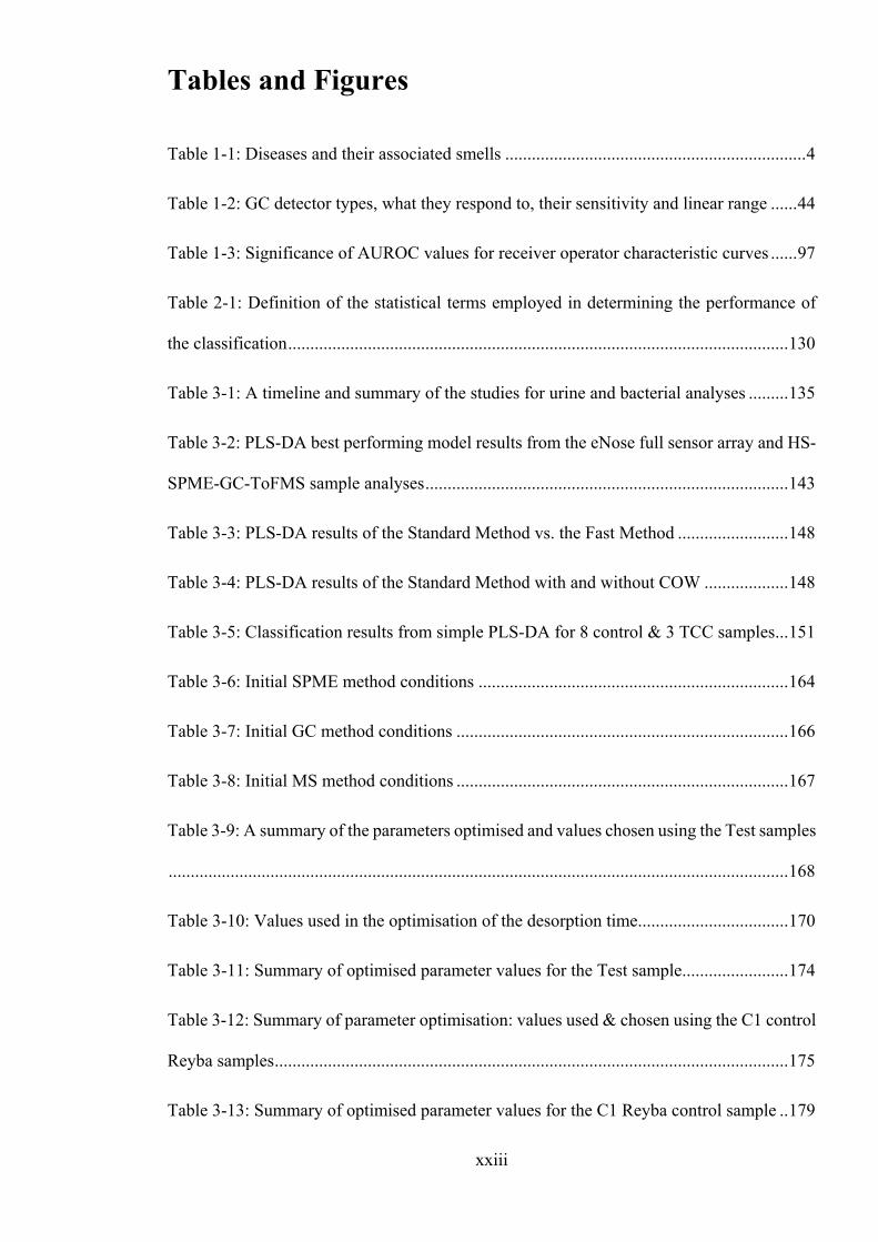
Tables and Figures

Table 1-1: Diseases and their associated smells .................................................................... 4

Table 1-2: GC detector types, what they respond to, their sensitivity and linear range ...... 44

Table 1-3: Significance of AUROC values for receiver operator characteristic curves ...... 97

Table 2-1: Definition of the statistical terms employed in determining the performance of

the classification ................................................................................................................. 130

Table 3-1: A timeline and summary of the studies for urine and bacterial analyses ......... 135

Table 3-2: PLS-DA best performing model results from the eNose full sensor array and HS-

SPME-GC-ToFMS sample analyses .................................................................................. 143

Table 3-3: PLS-DA results of the Standard Method vs. the Fast Method ......................... 148

Table 3-4: PLS-DA results of the Standard Method with and without COW ................... 148

Table 3-5: Classification results from simple PLS-DA for 8 control & 3 TCC samples ... 151

Table 3-6: Initial SPME method conditions ...................................................................... 164

Table 3-7: Initial GC method conditions ........................................................................... 166

Table 3-8: Initial MS method conditions ........................................................................... 167

Table 3-9: A summary of the parameters optimised and values chosen using the Test samples

............................................................................................................................................ 168

Table 3-10: Values used in the optimisation of the desorption time.................................. 170

Table 3-11: Summary of optimised parameter values for the Test sample ........................ 174

Table 3-12: Summary of parameter optimisation: values used & chosen using the C1 control

Reyba samples .................................................................................................................... 175

Table 3-13: Summary of optimised parameter values for the C1 Reyba control sample .. 179

xxiv

Table 3-14: Summary of the SPME fibre types and parameters ....................................... 181

Table 4-1: TCC and Control participants used in the study, no age-matching .................. 217

Table 4-2: Participants used in the study age, pH and specific gravity, no age-matching 218

Table 4-3: Participants used in the age-matched data set .................................................. 219

Table 4-4: Summary of the IS identification results for all samples ................................. 223

Table 4-5: Summary of the IS abundance and SN ratio data for all samples .................... 227

Table 4-6: Summary of the sample blanks IS identification results for all batches .......... 235

Table 4-7: Summary of the IS response in all sample blanks for all batches .................... 237

Table 4-8: IS carryover detected in the fibre blanks .......................................................... 249

Table 4-9: IS results for consecutive injections of a C3 sample from Batch 9 ................. 253

Table 4-10: IS results for consecutive injections of a C1 control sample in Batch 3 ........ 254

Table 4-11: IS results for in-batch replicate injections of a C1 sample in Batch 12 ......... 256

Table 4-12: IS results for between-batch injection of a C1 sample in Batches 9, 13 & 14

........................................................................................................................................... 258

Table 4-13: C1 vs. TCC results for PLS-DA and SVM-LIN ............................................ 262

Table 4-14: C2 vs. TCC results for PLS-DA and SVM-LIN ............................................ 263

Table 4-15: C3(full) vs. TCC results for PLS-DA and SVM-LIN .................................... 264

Table 4-16: C3(full) vs. TCC1 results for PLS-DA and SVM-LIN .................................. 266



Table 4-19: Comparison of classification algorithms across all datasets .......................... 286

Table 4-20: Comparison of the results using the C3(full) and C3(AM) data sets ............. 294

xxv

Table 4-21: Z-test statistical significance for overlapping distributions with PLS-DA ..... 296

Table 4-22: Potential biomarkers identified from the PLS-DA loadings after classification.

............................................................................................................................................ 298

Table 5-1: Participants used in the study: prostate cancer (PC) and control (C4 and BPH)....

...................................................................................................................... 312

Table 5-2: Participants used in the PC study: age, pH and specific gravity ...................... 313

Table 5-3: IS results for consecutive injections of a PC sample in Batch 1 ...................... 316

Table 5-4: IS results for in-batch replicate injections of a PC sample in Batch 2 ............. 318

Table 5-5: IS results for between-batch replicate injections of a BPH sample .................. 320

Table 5-6: Summary of performance obtained for the mean of the classification models 326

Table 6-1: Participants used in the study including patients with liver cirrhosis (CIR), with

and without HCV (HepC+ve or HepC-ve) and control (C) participants ........................... 340

Table 6-2: Participants used in the hepatic disorders study: age, pH and specific gravity 340

Table 6-3: Summary of the IS identification results .......................................................... 343

Table 6-4: Summary of the IS abundance and SN ratio data ............................................. 344

Table 6-5: Summary of the sample blanks IS identification results .................................. 346

Table 6-6: Summary of the sample blanks IS abundance and SN ratio data ..................... 347

Table 6-7: Carryover of the IS detected in the fibre blanks ............................................... 350

Table 6-8: IS results for consecutive injections of a CON sample in Batch 5 ................... 352

Table 6-9: IS results for in-batch replicates of a CIRHepC-ve sample in Batch 1 ............ 353

Table 6-10: IS reproducibility for between-batch replicates of a CIRHepC-ve sample .... 355

Table 6-11: CIRHepC-ve vs. CON using PLS-DA, SVM and ANNs ............................... 358

Table 6-12: CIRHepC+ve vs. CON & CIRHepC-ve using PLS-DA, SVM and ANNs .... 362

xxvi

Table 6-13: CIRHepC+ve vs. balanced CON & CIRHepC-ve using PLS-DA, SVM and

ANNs ................................................................................................................................. 366

Table 7-1: Summary of number of samples of each type analysed by HS-GC-MS .......... 375

Table 7-2: Summary of samples and conditions in the analysis by HS-GC-MS ............... 376

Table 7-3: Summary of number of samples of each type analysed by TD-GC-MS .......... 377

Table 7-4: Summary of samples and conditions in the analysis by TD-GC-MS. ............. 378

Table 7-5: Carryover peak data ........................................................................................ 386

Table 7-6: Plan for follow-on sepsis study ........................................................................ 400

Figure 1.1: Model of theoretical plates in an analytical column of fixed length (cm); (a) few

theoretical plates and large plate height; (b) many theoretical plates and small plate height

............................................................................................................................................. 33

Figure 1.2: Graph of HETP (H) against linear velocity for an uncoated capillary column . 35

Figure 1.3: Resolution and selectivity of chromatographic peaks ....................................... 36

Figure 1.4: Measurements on the chromatogram used in the calculation of (a) resolution,

(b)selectivity and capacity factor ......................................................................................... 37

Figure 1.5: Van Deemter plot of HETP against average linear velocity through the column

for nitrogen, helium and hydrogen carrier gases ................................................................. 39

Figure 1.6: Neutral molecules elute from the GC column and are hit by an electron with

70eV, knocking out an electron. The radical cation may then fragment. ............................ 47

Figure 1.7: Time-of-Flight mass analyser ........................................................................... 50

xxvii

Figure 1.8: Example of a 2D contour plot of diesel by GCxGC-FID: x-axis 1st dimension

retention time (s); y-axis 2nd dimension retention time (s); colour represents response: from

no response (dark blue) to highest response (red). ............................................................... 60

Figure 1.9: Example of a 3D surface plot of diesel by GCxGC-FID ................................... 61

Figure 1.10: Example of a 2D chromatogram of diesel by GC-FID .................................... 61

Figure 1.11: The stages of GCxGC. Acknowledgements to JSB UK for their kind permission

to use their diagram .............................................................................................................. 62

Figure 1.12: Receiver Operator Curves (ROC) showing AUROC values and significance 96

Figure 2.1: Flow diagram of sample vial preparation ........................................................ 106

Figure 2.2: Diagram of the sampling set-up for the BACTECTM bottle ............................ 117

Figure 2.3: A visual representation of the 3-dimensional (3D) GC-MS data: x-axis = scan

number or retention time (min or s); y-axis = intensity (arbitrary units, value manufacturer

dependent); z-axis = m/z (u) .............................................................................................. 121

Figure 2.4: Extraction of a 2D mass spectrum from the 3D data matrix for a certain scan

number or retention time: x-axis = m/z (u); y-axis = intensity (arbitrary units, manufacturer

dependent or can be normalised to the most abundant ion (%)) ........................................ 122

Figure 2.5: Extracted Ion Chromatogram (EIC) of the intensity of a certain m/z plotted

against the scan number or retention time (min or s) ......................................................... 122

Figure 2.6: Creation of a 2D Total Ion Chromatogram (TIC) from the 3-D GC-MS data,

where the abundances of all ions for each scan number are summed to produce a TIC: x-axis

= scan number or retention time (min or s); y-axis = intensity of summed ions (arbitrary

units, manufacturer dependent) .......................................................................................... 123

Figure 2.7: Alignment prior to chromatogram comparison ............................................... 125

Figure 2.8: Workflow of the chemometric data processing ............................................... 129

xxviii

Figure 3.1: Scores scatter plot after PLS-DA analysis of 5 bladder cancer positive and 10

bladder cancer negative samples from the preliminary work. Score t1 (first component)

explains largest variation in the data set, followed by t2, etc. Red circle shows the

aggregation of the 5 positive samples. ............................................................................... 138

Figure 3.2: Simple PCA score plot for 2 TCC and 4 control samples by GCxGC ........... 152

Figure 3.3: Optimisation of analyte extraction time from Test samples ........................... 169

Figure 3.4: Optimisation of fibre desorption time from Test samples .............................. 170

Figure 3.5: Optimisation of incubation speed from Test samples ..................................... 172

Figure 3.6: Optimisation of pre-incubation time and temperature from Test samples ...... 173

Figure 3.7: TICs of the fibre blanks from Test sample bakeout time optimisation ........... 173

Figure 3.8: Optimisation of extraction time using the C1 control Reyba samples ............ 176

Figure 3.9: TICs of the fibre blanks from Reyba C1 control sample bakeout time optimisation

........................................................................................................................................... 177

Figure 3.10: TICs of the C1 Reyba control samples from the desorption time optimisation

........................................................................................................................................... 178

Figure 3.11: Overlaid TICs of the fibre blanks for the three SPME fibres ....................... 182

Figure 3.12: Overlaid chromatograms of blanks (with no IS added) for the SPME fibres 183

Figure 3.13: TICs from the PDMS/DVB fibre analysis of a C1 Goutr control ................. 185

Figure 3.14: TICs from the PDMS fibre analysis of a C1 Goutr control .......................... 185

Figure 3.15: TICs from the CAR/PDMS fibre analysis of a C1 Goutr control ................. 186

Figure 3.16: TICs of the e analysis of C1 Goutr control samples using different SPME fibres

........................................................................................................................................... 186

Figure 3.17: Comparison of column bleed between the SGE and Restek columns .......... 188

xxix

Figure 3.18: TICs of the HS sampling of laboratory air vs. BACTEC bottle .................... 192

Figure 3.19: EIC m/z 149 of HS sampling of laboratory air with & without a microbial filter

............................................................................................................................................ 193

Figure 3.20: EIC m/z 43 u for the HS analysis of laboratory air with microbial filter ...... 193

Figure 3.21: TICs of the TD sampling of laboratory air vs. BACTEC bottle ................... 197

Figure 3.22: EICs m/z 43 and 57 u for the TD analysis of laboratory air with the microbial

filter .................................................................................................................................... 198

Figure 4.1: A snapshot of the metadata for TCC2 and TCC3 participants, showing sex, age,

smoker and urinalysis results ............................................................................................. 208

Figure 4.2: A snapshot of the metadata for Control 2 participants, showing diagnosis and

medication taken within 48 hours prior to study ................................................................ 209

Figure 4.3: A snapshot of the metadata for Control 3 participants, showing food and drink

intake during 48 hours prior to study ................................................................................. 210

Figure 4.4: Plot of IS retention time for all samples .......................................................... 224

Figure 4.5: Plot of the IS retention time for all samples after outlier removal .................. 225

Figure 4.6: The IS retention time for batches after outlier removal, showing the downward

linear trendline ................................................................................................................... 226

Figure 4.7: Plot of the average IS area and RSD (%) for each batch ................................. 228

Figure 4.8: The IS quantitation ion peak area for Batch 1 ................................................. 228

Figure 4.9: The IS quantitation ion peak areas for Batch 2 ............................................... 229

Figure 4.10: The IS quantitation ion peak areas for Batch 3 showing a linear trendline ... 230

Figure 4.11: The IS quantitation ion peak areas for Batch 8 ............................................. 231

xxx

Figure 4.12: The IS quantitation ion peak areas for Batch 14 showing the linear trendline

........................................................................................................................................... 231

Figure 4.13: The IS quantitation ion peak areas for the remaining batches ...................... 233

Figure 4.14: Plot of the IS average SN ratio and RSD (%) for each batch ....................... 233

Figure 4.15: The IS retention time in all sample blanks .................................................... 236

Figure 4.16: The IS peak area average and RSD (%) for all samples and sample blanks . 238

Figure 4.17: Plot of IS peak area and similarity match for all sample blanks ................... 239

Figure 4.18: Overlaid TICs of Injection 1 Fibre blanks for all batches ............................. 240

Figure 4.19: Overlaid TICs of Injection 1 (orange) & 2 (green) Fibre blanks from Batch 9

........................................................................................................................................... 241


........................................................................................................................................... 242

Figure 4.21: Overlaid Injection 2 Matrix blank TICs from Batches 2, 4-6, 8-9, 12, 14, 16-22

........................................................................................................................................... 243

Figure 4.22: Overlaid Injection 1 Fibre blank & Injection 2 Matrix blank TICs in Batch 21

........................................................................................................................................... 244

Figure 4.23: Overlaid Injection 2 Procedural blank TICs in Batches 1, 3, 7, 10-11, 13 & 15

........................................................................................................................................... 245

Figure 4.24: Overlaid Injection 2 Batch 7 & 11 Procedural & Batch 21 Matrix blank TICs

........................................................................................................................................... 246

Figure 4.25: Overlaid Batch 13 C3 sample with Injection 2 Batch 11 Procedural and Batch

21 Matrix blank TICs ......................................................................................................... 247

Figure 4.26: Percentage carryover determined from fibre blank injections ...................... 250

xxxi

Figure 4.27: Zoomed-in IS quantitation ion showing a low percentage carryover ............ 251

Figure 4.28: Zoomed-out IS quantitation ion showing a low percentage carryover of the IS

............................................................................................................................................ 251

Figure 4.29: IS quantitation ion for consecutive injections of a C3 sample from Batch 9 253

Figure 4.30: IS quantitation ion for consecutive injections of a C1 sample in Batch 3 ..... 254

Figure 4.31: Overlaid TICs of three consecutive injections of a TCC3 sample in Batch 20

............................................................................................................................................ 255

Figure 4.32: IS quantitation ion for in-batch replicate injections of a C1 sample in Batch 12

............................................................................................................................................ 256

Figure 4.33: Overlaid TICs of three in-batch injections of a TCC1 sample in Batch 10 ... 257

Figure 4.34: IS quantitation ion for between-batch injections of a C1 sample in Batches 9,

13 & 14 ............................................................................................................................... 258

Figure 4.35: Overlaid TCC2 sample TICs of between-batch injections in Batches 1, 7 & 18

............................................................................................................................................ 259

Figure 4.36: Permutation density plots for C1 vs. TCC using (a) PLS-DA, (b) SVM-LIN, (c)

RFs .................................................................................................................. 274


RFs ..................................................................................................................................... 275

Figure 4.38: Permutation density plots for C3(full) vs. TCC using (a) PLS-DA, (b) SVM-

LIN, (c) RFs ....................................................................................................................... 277

Figure 4.39: Density plots of TCC vs. C1/C2/C3 for PLS-DA, SVM-LIN and RFs ........ 278

Figure 4.40: Permutation density plots for C3(full) vs. TCC1 using (a) PLS-DA, (b) SVM-

LIN, (c) RFs ....................................................................................................................... 280

xxxii


LIN, (c) RFs ....................................................................................................................... 282


LIN, (c) RFs ....................................................................................................................... 283

Figure 4.43: Density plots C3(full) vs. TCC1/2/3 for PLS-DA, SVM-LIN and RFs ........ 285

Figure 4.44: Permutation density plots for C3(AM) vs. TCC using (a) PLS-DA, (b) SVM-

LIN, (c) RFs ....................................................................................................................... 288

Figure 4.45: Permutation density plots for C3(AM) vs. TCC1 using (a) PLS-DA, (b) SVM-

LIN, (c) RFs ....................................................................................................................... 289


LIN, (c) RFs ....................................................................................................................... 290


LIN, (c) RFs ....................................................................................................................... 291

Figure 4.48: Permutation density plots of the C3(AM) data set against all TCC data and the

TCC1 data set .................................................................................................................... 292

Figure 4.49: Permutation density plots of the C3(AM) data set against the TCC1 and TCC2

data sets .............................................................................................................................. 293

Figure 4.50: PRS PLS-DA Loading Viewer suggesting retention times of key peaks in the

C3(AM) vs. TCC1 classification ....................................................................................... 297

Figure 5.1: Snapshot of metadata for prostate cancer (PC) participants, showing sex, age,

smoker plus urinalysis results ............................................................................................ 307

Figure 5.2: Snapshot of metadata for BPH participants, showing diagnosis and medication

taken within 48 hours prior to study .................................................................................. 308

xxxiii

Figure 5.3: Snapshot of metadata for C4 participants, showing food and drink intake during

48 hours prior to study ....................................................................................................... 309

Figure 5.4: IS (peak 2) quantitation ion for consecutive injections of a Batch 1 PC sample ..

.................................................................................................................. 316

Figure 5.5: Overlaid TICs of consecutive injections of a BPH sample in Batch 2 ............ 317

Figure 5.6: IS quantitation ion for in-batch replicates of a PC sample in Batch 2 ............. 318

Figure 5.7: Overlaid TICs of in-batch replicates of a C4 sample in Batch 14 ................... 319

Figure 5.8: IS quantitation ion for between-batch injections of a BPH sample in Batches 8,

11 & 18 ............................................................................................................................... 320

Figure 5.9: Overlaid TICs of between-batch replicates of a BPH sample ......................... 321

Figure 5.10: Permutation density plots for C4 vs. PC using PLS-DA ............................... 324

Figure 5.11: Permutation density plots for C4 vs. BPH using PLS-DA ............................ 325

Figure 5.12: Permutation density plots for BPH vs. PC using PLS-DA ............................ 326

Figure 5.13: Possible future care pathway for patients with suspected prostate cancer with

the HS-SPME-GC-MS chemometric urine sample analysis .............................................. 331

Figure 6.1: Snapshot of metadata for CIRHepC-ve participants, showing sex, age, smoker

plus urinalysis results ......................................................................................................... 336

Figure 6.2: Snapshot of metadata for CIRHepC-ve and HepC+ve participants, showing

fibrosis score and medication taken within 48 hours prior to study .................................. 337

Figure 6.3: Snapshot of metadata for some Control participants, showing food and drink

intake during 48 hours prior to study ................................................................................. 338

Figure 6.4: Plot of IS retention time for all samples .......................................................... 343

Figure 6.5: Variation in the peak area of the IS quantitation ion for all samples .............. 345

xxxiv

Figure 6.6: IS peak area for Batch 1 with an exponential trendline fitted ......................... 346

Figure 6.7: IS quantitation ion peak area for procedural blanks ........................................ 348

Figure 6.8: The overlaid TICs of Injection 1 Fibre blanks ................................................ 349

Figure 6.9: The overlaid TICs of Injection 2 Procedural blanks ....................................... 349

Figure 6.10: IS quantitation ion for consecutive injections of a CON sample in Batch 5 . 351

Figure 6.11: Overlaid TICs of consecutive injections of a CIRHepC-ve sample in Batch 4

........................................................................................................................................... 352

Figure 6.12: IS quantitation ion for in-batch replicates of a Batch 1 CIRHepC-ve sample

........................................................................................................................................... 353

Figure 6.13: Overlaid TICs of in-batch replicates of a CIRHepC+ve sample in Batch 4 . 354

Figure 6.14: IS quantitation ion for between-batch replicates of a CIRHepC-ve sample . 355

Figure 6.15: TICs of between-batch replicates of a CIRHepC-ve sample in Batches 1, 4 & 5

........................................................................................................................................... 356

Figure 6.16: Permutation density plots for CIRHepC-ve vs. CON using (a) PLS-DA, (b)

SVM-LIN, (c) SVM-RBF .................................................................................................. 360

Figure 6.17: Permutation density plots for CIRHepC-ve vs. CON using ANNs with PNNs

(a) without feature selection, (b) with feature selection .................................................... 361

Figure 6.18: Permutation density plots for CIRHepC+ve vs. CON & CIRHepC-ve using (a)

PLS-DA, (b) SVM-LIN, (c) SVM-RBF ............................................................................ 364

Figure 6.19: Permutation density plots for CIRHepC+ve vs. CON & CIRHepC-ve using

ANNs with PNNs (a) without feature selection, (b) with feature selection. ..................... 365

Figure 6.20: Permutation density plots for CIRHepC+ve vs. balanced CON & CIRHepC-ve

using (a) PLS-DA, (b) SVM-RBF, (c) ANNs ................................................................... 367

xxxv

Figure 7.1: TICs of HS-GC-MS blanks (a) syringe; (b) aerobic bottle; (c) anaerobic bottle

............................................................................................................................................ 380

Figure 7.2: TICs of HS-GC-MS (a) aerobic blank; (b) aerobic Staph. aureus + alpha haem.

strept. .................................................................................................................................. 381

Figure 7.3: Comparison of Anaerobic (red) and Aerobic (blue) bottle blanks against

instrument (black) and TD tube (green) blanks ................................................................. 383

Figure 7.4: Carryover check for anaerobic bacteria ........................................................... 385

Figure 7.5: Zoomed in comparison of an aerobic sample vs. blank aerobic bottle by TD-GC-

MS ...................................................................................................................................... 388

Figure 7.6: Zoomed in comparison of all aerobic samples by TD-GC-MS ....................... 390

Figure 7.7: Zoomed in comparison of an anaerobic sample vs. blank anaerobic bottle by TD-

GC-MS ............................................................................................................................... 392

Figure 7.8: Zoomed in comparison of all anaerobic samples by TD-GC-MS ................... 393

Figure 7.9: PCA plot of the HS samples ............................................................................ 395

Figure 7.10: HCA dendrogram of the HS samples ............................................................ 396

Figure 7.11: PCA analysis of data files from TD-GC-MS, no scaling .............................. 396

Figure 7.12: HCA dendrogram of the TD samples and blanks .......................................... 397

Figure 7.13: Timetable for follow-on sepsis study ............................................................ 399

1

Introduction

2

1. Aims

The aim of the thesis is to develop and evaluate the performance of non-invasive methods to

characterise the disease states of patients utilising selective discrimination, gas

chromatography-mass spectrometry and chemometrics.

The primary analytical method to be investigated is gas chromatography-time-of-flight mass

spectrometry coupled with solid-phase microextraction. The hypothesis is:

i) As previously demonstrated by dogs, the headspace above a urine sample will

contain a profile of volatile organic compounds that can be utilised to diagnose

the presence or absence of disease.

ii) The sampling method parameters and the SPME fibre coatings can be optimised

to reproducibly extract a wide range of volatile organic compounds from the

headspace above complex matrices, such as urine.

iii) Harnessing the separating power of gas chromatography will enable very similar

compounds to be resolved temporally, enabling the wide range of volatile organic

compounds to be characterised and their abundance to be compared between

samples.

iv) Coupling of the chromatography eluent with the fast acquisition rate of a time-

of-flight mass spectrometer further enhances the resolving power, by enabling

the capture of the full mass spectrum at such a rate that peak deconvolution is

also possible.

v) Analysis of the rich data sets produced, by bespoke algorithms, will allow the

disease state of a patient to be accurately determined.

3

1.1 Background

The ‘smell’ of illness, disease or age has been known for many centuries, with some smells,

such as stale sweat, mucus and cough medicine being easily identifiable as likely to be from

someone with a bad cold or flu. Whereas, other smells, much like those associated with

decay, indicate that someone doesn’t smell ‘right’ without knowing the cause - illness or

disease. Some diseases and their associated smells are listed in Table 1-1 (Wilson & Baietto,

2011).

Until recently, malodour hasn’t been investigated for use in clinical medicine as a

quantifiable diagnostic tool, to tell if someone is sick or to diagnose which illness or disease

that person suffers from (Kusuhara, et al., 2010). There are notes in medical textbooks

referring to the fact that patient odour is useful, particularly in the diagnosis of congenital

metabolic diseases in infants. An example is Maple Syrup disease, where the urine is very

sweet smelling, like maple syrup, after birth (NHS Choices information, 2015). However, it

is mainly in the last couple of decades that ‘smell’ has been investigated as a diagnostic tool

and clinicians have gathered evidence in a scientific manner (Wilson & Baietto, 2011). The

profiles of volatile organic compounds (VOCs) are increasingly being utilised as non-

invasive diagnostic methods for determining the presence, or absence, of an illness or

disease.

Smells are created by volatile compounds, usually with a low molecular weight of 350 g or

less. Olfactory detection is the term that covers the study of compounds responsible for

smell and it has been widely applied in the food and fragrance sector, with over 8,000

volatiles detected and identified; however, less than 5 % of these compounds contributed to

the aromas of these foods (Grosch, 2001).

4

Table 1-1: Diseases and their associated smells

Disease/ Disorder Body source Descriptive aroma Acromegaly Body Strong, offensiveAnaerobic infection Skin, sweat Rotten applesAzotemia (prerenal) Urine Concentrated urine odourBacterial proteolysis Skin Over-ripe CamembertBacterial vaginosis Vaginal discharge Amine-likeBladder infection Urine Ammonia Bromhidrosis Skin, nose UnpleasantDarier’s disease Buttocks Rank, unpleasant odourDiabetic ketoacidosis Breath Rotting apples, acetoneCongestive heart failure Heart (portcaval shunts) Dimethyl sulphideCystic fibrosis Infant stool FoulDiabetes mellitus Breath Acetone-likeDiphtheria Sweat SweetEmpyema (anaerobic) Breath Foul, putridEsophageal diverticulum Breath Feculent, foulFetor hepaticus Breath Newly-mown clover, sweetGout Skin Gouty odourHydradenitis suppurativa Apocrine sweat glands Bad body odourHyperhydrosis Body Unpleasant body odourHyperaminoaciduria Infant skin Dried malt or hopsHypermethioninemia Infant breath Sweet, fruity, fishy, boiled cabbage, rancid

butterIntestinal obstruction Breath Feculent, foulIntranasal foreign body Breath Foul, feculentIsovaleric academia Skin, sweat, breath Sweaty feet, cheesyKetoacidosis (starvation) Breath Sweet, fruity, acetone-likeLiver failure Breath Musty fish, raw liver, mercaptans, dimethyl

sulphideLung abscess Sputum, breath Foul, putrid, fullMaple syrup urine disease Sweat, urine, ear wax Maple syrup, burnt sugarPhenylketonuria Infant skin Musty, horsey, mousy, sweet urine Pneumonia (necrotizing) Breath PutridPseudomonas infection Skin, sweat GrapeRenal failure (chronic) Breath Stale urineRotavirus gastroenteritis Stool FullRubella Sweat Freshly plucked feathersSchizophrenia Sweat Mildly aceticScrofula Body Stale beerScurvy Sweat PutridShigellosis Stool RancidSmallpox Skin Pox stenchSquamous-cell carcinoma Skin Offensive odourSweaty feet syndrome Urine, sweat, breath Foul aceticTrench mouth Breath HalitosisTrimethylaminuria Skin, urine FishyTB lymphadenitis Skin Stale beerTubular necrosis (acute) Urine Stale waterTyphoid Skin Freshly-baked brown breadUremia Breath Fishy, ammonia, urine-likeVagabond’s disease Skin UnpleasantVaricose ulcers, malignant Leg Foul, unpleasantYellow fever Skin Butcher’s shop

5

Volatile compounds can emerge from the body in several ways including: excretion in the

breath; secretions from the skin as sweat; secretions from mucous membranes in the nose,

mouth, ears and urogenital area; and excretion in the urine and faeces. In the 1960s rats were

trained to differentiate the sweat between schizophrenic patients and non-schizophrenic

people (Smith, et al., 1969) and the compound was reportedly isolated and identified by gas

chromatography-mass spectrometry (GC-MS) and nuclear magnetic resonance (NMR).

Various reports followed, with a paper published in 2005 (Di Natale, et al., 2005) which

reported that no single biomarker could be identified to differentiate between the three

sample classes of schizophrenics, other mental disorders and controls using GC-MS and a

chemical sensor array. However, by considering the whole sample the classification could

be achieved.

There has been much research studying breath in recent years, with around 3,000 volatile

organic compounds (VOCs) being detected in breath but only 20-30 of these being present

in all humans (Phillips, et al., 1999). Numerous examples of conditions which induce VOC

changes, often manifested through odour in the breath, have been documented. Arguably

the most familiar breath analysis application is the diagnosis of diabetic ketoacidosis, where

the breath acquires a characteristic ‘pear drop’ odour (Probert, et al., 2009). However, lung

cancer (Horvath, et al., 2009), breast cancer (Philips, et al., 2006), gastric cancer (Amal, et

al., 2015), colorectal cancer (Amal, et al., 2016) and other diseases (Lourenco & Turner,

2014) have also been studied, .

The excreted or secreted odorous compounds causing the smell can be because of the intake

of chemicals into the body. For example, eating garlic or smoking. They can also be caused

by chemical reactions occurring inside the body caused by bacteria, cancers and diseases.

Cancer is the largest cause of death in the world, with malignant neoplasms causing 7.87

million deaths in 2011, compared to 7.02 million caused by ischaemic heart disease and 6.25

6

million caused by stroke (World Health Organization, 2014). Cancer causes changes in

genes, which results in changes to the proteins and enzymes within the cells that eventually

produce modified metabolites. These metabolites are then excreted from the body through

urine or from the lungs in the patient’s breath, or can be secreted from the skin and mucous

membranes. Endogenous bacteria, within different organs within the body, can also

metabolise some of these modified metabolites, producing different volatile organic

compounds (VOCs). These metabolites can differ, depending on which organ the cancerous

cells are present in, and hence can be a route to determining which cancer type is present.

Necrosis or tissue death from the cancer can also produce volatile compounds (Mazzone,

2008).

Bacterial cultures produce hundreds of volatile compounds. In the past, the unique smells

of different bacteria enabled identification, for example Pseudomonas aeruginosa smells

like grapes, Streptococcus anginosus smells like caramel or butterscotch, Clostridium

difficile like a ‘barnyard’ and other anaerobic and enteric bacteria (from the intestines) like

Salmonella smell terrible (Bawdon, et al., 2015). On the body, bacteria make humans smell

‘bad’, for example Staphylococcus hominis is responsible for the body odour (BO) smell

when sweat is digested by this bacterium on the skin (Bawdon, et al., 2015).

In humans, olfactory detection of volatile compounds is through olfactory receptors in the

nasal cavity. The volatile compounds in the air dissolve into the mucus and bind with the

receptors. There are 390 known functional olfactory receptor genes in humans and 299

subfamilies; however, in dogs there are 872 genes and 300 subfamilies (Niimura & Nei,

2006). Humans have around 10 million olfactory cells with 8-12 microvilli (microscopic

cellular membrane protrusions) each, whereas dogs have around 200 million cells with

around 125 microvilli each. However, the number of receptors, cells and microvilli is

reportedly not a definitive indicator of how good the species is at detecting smells (Shepherd,

2004), as it is also attributed to the perception and recognition of the smell by the brain.

7

Dogs have been used in many roles, that rely on their excellent sense of smell. ‘Sniffer’

dogs have been trained to detect explosives, illegal drugs, arson, food, human remains and

even bed bugs (Lewis, et al., 2013).

Dogs were first reported to be able to detect cancer in a report in the Lancet in 1989

(Williams & Pembroke, 1989), where a dog discovered a malignant melanoma. Since then,

dogs have been trained to detect cancer by sniffing the headspace above the urine of bladder

cancer patients. Willis and colleagues (Willis, et al., 2004) trained six dogs of varying ages

and breeds to distinguish between urine samples from 36 male and female patients suffering

from new or recurrent transitional cell carcinoma of the bladder (TCC) and 108 male and

female controls, who were healthy or were diseased but did not have bladder cancer.

Twenty-seven of the TCC samples and 54 control samples were used in the training. The

remaining 9 TCC samples and 54 control samples were used in the evaluation. The aim was

to train the dogs to identify the urine from the bladder cancer patients based on the cancer

status alone, rather than the secondary effects of bleeding, inflammation, infection and

necrosis. Six dogs of different breeds and ages were trained over 7 months. For the

evaluation, one TCC sample was placed amongst six control samples and each dog assessed

for correctly selecting the TCC sample. Nine test panels, each with one bladder cancer and

six control samples, were run, giving a total of 54 assessments in all. The dogs used their

highly acute sense of smell and their ability to recognise complex patterns to correctly select

the urine from bladder cancer patients on 22 out of 54 occasions giving a 41 % mean success

rate. With 95 % confidence intervals (CI) giving values of 23-58 % under assumptions of

normality and 26-52 % from bootstrap methods. This finding was much higher than a

determined success rate of 14 %, based on chance alone. Multivariate analysis indicated that

the dogs could detect volatiles coming from the bladder cancer rather than other chemicals

detectable by urinalysis. Therefore, this seminal proof of principle study was deemed to be

successful.

8

However, the accuracy, sensitivity and reproducibility is dog dependent and dogs can’t

currently be used in a clinical setting. Commercial analytical instruments can be configured

to mimic the sampling and pattern recognition capabilities of dogs and distinguish between

patients presenting with a disease and those without. To replace dogs with an analytical

instrument, capable of analysing the volatile organic compounds from urine samples, then

we would need to develop a method that is:

• Accurate and specific, to correctly identify the disease;

• Reproducible, day in and day out with no ‘off’ days;

• Sensitive, to obtain early diagnosis for a better prognosis;

• A fast analysis, to obtain an answer quickly and at lower cost;

• Suitable as a routine screen for diseases.

There are now multiple different techniques reported for analysing VOCs for the detection

of cancer (Haick, et al., 2014). Cross-reactive nanoarrays combined with pattern recognition

have been used for the detection of precancerous gastric lesions and gastric cancer (Amal,

et al., 2015) and colorectal cancer (Amal, et al., 2016) through exhaled breath. There are

several problems, when using breath samples as a diagnostic tool for cancer and diseases,

these include: the interferences from exogenous volatiles from the air, food and smoking

(Horvath, et al., 2009); the low concentration of VOCs in breath and the level of water

vapour within the samples. Amal and colleagues collected two samples (750 mL GaSampler

collection bag) of exhaled breath, after the patient had inhaled through a filter cartridge for

3 minutes, to minimise exogenous VOCs. The alveolar air from the lungs, was collected

into a separate bag and then the contents were transferred and concentrated onto a thermal

desorption (TD) tube containing two hydrophobic sorbents, so that the water vapour was not

trapped. One TD tube was analysed by GC-MS and the other by the cross-reactive

nanoarrays. The nanoarrays consisted of eight sensors based on either organically-stabilised

9

spherical gold nanoparticles (GNPs) or single-walled carbon nano-tubes (SWCNTs) covered

with different ligands. The TD tube was heated and the vapour stored in a heated metal

column until it was sucked into a vacuum chamber containing the sensors. The ligands on

the different sensors then adsorbed different VOCs, generating different electrical signals

that were recorded. The data was then analysed using chemometrics.

Selected-ion flow-tube MS (SIFT-MS) has recently been reported for the detection of

cancers through breath analysis (Kumar, et al., 2015), along with other applications (Smith

& Spanel, 2015). SIFT-MS analyses the sample directly, in real-time, with no

chromatographic separation. It produces soft ionisation, with little fragmentation of the

molecule and works well in a well-characterised matrix. However, when analysing complex

matrices there are many masses that overlap, resulting in isobaric interference and the

incorrect quantification of compounds. It is also believed that the sensitivity is not high

enough for many trace compounds present in breath (Smith & Spanel, 2015).

GC-MS is an analytical technique that has been successfully used for the separation and

detection of volatile organic compounds for decades. In more recent years, GC-MS is one

of the fundamental techniques (Childs & Williams, 2014), along with LC-MS, that has been

adopted and used in metabolomics profiling, the study of small molecule metabolites that

are produced by and influence cellular processes. It is utilised to learn about cellular biology,

systems biology and disease. Metabolomics is mostly used in the study of plants in the agro-

biotechnology field (Hall & Hardy, 2012) and in the biomedical industry looking at health

and disease in humans and animals (Weckwerth, 2006).

GC-MS is a highly sensitive and selective analytical technique for resolving and identifying

large numbers of organic compounds present in complex samples. By carefully choosing

the sampling and sample introduction techniques, used to transfer the analytes into the GC,

the volatility and nature of the compounds can be selected to only introduce the compounds

10

of interest while leaving behind matrix and any interferents within the sample. The flexibility

of this capability is key when analysing urine and blood samples. Analytes eluting from the

GC are already in the gas-phase and are therefore compatible with the mass spectrometer for

qualitative or quantitative analysis. The parameters in the MS can be chosen to either detect

target compounds selectively with high sensitivity or to rapidly collect large amounts of data

looking at all the compounds separated by the GC, which may be many hundreds.

Chemometric techniques are then used to extract information from the GC-MS or LC-MS

data. For example, to identify patterns or classes within a data set. It is particularly useful

where the data set is large or contains large amounts of information. Clinical samples

generally are complex, containing organic compounds with a wide volatility range as well

as inorganic compounds.

The potential of using GC-MS as a non-invasive, sensitive diagnostic method to characterise

diseases will be investigated in this thesis, through the utilisation of a combination of:

• Selective discrimination, to select the optimal sampling and sample introduction

techniques;

• Gas chromatography, to separate the selected analytes;

• Mass spectrometry, to detect all the resolved analytes;

• Chemometrics, to identify differences between the clinical samples

The approach explored will include the development of the methodology to analyse the

headspace above urine samples and its application and evaluation for the diagnosis of

bladder cancer, prostate cancer and hepatic disorders and a separate method for the analysis

of the headspace above bacteria, for the classification of septic infection. A brief introduction

to each of the clinical areas of study will be provided in Section 1.2.

11

1.2 A background to the clinical areas of study in this thesis

1.2.1 Bladder cancer

There are over 200 different types of cancer; bladder cancer is the ninth most common cancer

worldwide and the thirteenth most common cause of cancer death (World Health

Organization, 2014). In the UK, it is the eighth most common type (Office for National

Statistics, 2014) and the seventh most common cause of cancer death (Cancer Research UK,

2014). Transitional cell carcinoma (TCC), also known as urothelial cell carcinoma (UCC),

is the most common type of bladder cancer, accounting for >90 % of cases in 2014.

1.2.1.1 Transitional cell carcinoma

TCC begins in the cells, called transitional cells, of the bladder wall or lining called the

urothelium (Bassi, et al., 2005). These cells come into contact with waste products in the

urine that may cause cancer, such as the chemicals in tobacco smoke which are a known

cause of bladder cancer (World Health Organization, 2014). Bladder cancer tumour staging

is based on the extent of penetration into the bladder wall and adjacent structures.

Superficial, otherwise known as early or non-muscle invasive, bladder cancer, is a cancer

that has not invaded the bladder smooth muscle. It includes the following stages: Ta is non-

invasive papillary carcinoma that appear as small, removable growths; Tis is carcinoma in-

situ (CIS) where the growths come back after removal; and T1 is where the tumour starts to

grow into the sub-epithelial connective tissue beneath the bladder lining. Stage 2 tumours

and higher are muscle-invasive: T2 is where the cancer has grown into the muscle; T3 is

where the cancer has grown through the muscle into the fat layer; and T4 is where the cancer

has grown outside of the bladder. Approximately 70-80 % of newly diagnosed TCCs present

as non-invasive and low-grade tumours and after treatment 50-70 % of these tumours recur

12

and require further treatment, with 10-20 % progressing to invasive tumours, despite

improvements in diagnosis and treatment. Invasive tumours in the muscle quickly progress

and metastasize, they have poor prognosis with only 30-40 % of patients surviving for longer

than five years. Therefore, the earlier bladder cancer can be diagnosed, if possible before

symptoms appear, the better the prognosis.

1.2.1.2 Bladder cancer diagnosis

Usually, the first indication of bladder cancer is blood in the urine (haematuria). This is

confirmed by carrying out urinalysis that can detect small amounts of blood, at which point

a cystoscopy is arranged. Cystoscopy is the gold standard for the diagnosis of bladder cancer

and is reliable. However, it uses invasive techniques to obtain a biopsy, which is both a

higher risk and causes discomfort for the patient. It is also expensive, at around £400 per

patient, when one considers that only around 20 % of haematuria patients have bladder

cancer. Infections are the most common causes of haematuria (NHS Choices, 2015).

Urine cytology can also be used to look for cancer cells using a microscope. It can be very

specific to identify the type of cancer (90-96 %), but it suffers from low sensitivity (20-50

%) (Bassi, et al., 2005). It requires an expert to interpret the results, can take several days to

get an answer and is not recommended for routine screening. More recent tests have been

approved; for example, looking for chromosome changes, various bladder tumour-

associated antigens, such as BTA (Glas, et al., 2003) or proteins in the urine (Poulakis, et

al., 2001). Although they are more sensitive, with reported sensitivities of 50-70 % and 50-

85 % respectively, they have poorer specificity (60-70 %) when compared to cytology. This

can result in false positives and false negatives and they are now not being recommended

for routine screening (American Cancer Society, 2016). Therefore, an early screening test

is required that is sensitive, specific, non-invasive and is inexpensive.

13

1.2.1.3 Diagnosis of bladder cancer using analytical chemistry

Since the publication by Willis and colleagues, there have been multiple studies published

involving the diagnosis of bladder cancer using non-invasive urinary metabonomics - the

quantitative measurement of the metabolic response to the pathophysiological stimuli.

Pasikanti and colleagues analysed samples from 24 bladder cancer patients and 51 controls

using a lengthy sample preparation method involving derivatisation followed by a liquid

injection into a GC-ToFMS. They reported 100 % sensitivity and specificity, compared to

33 % sensitivity and 100 % specificity for urine cytology (Pasikanti, et al., 2010). However,

the study was unclear about the type of controls used, there was no mention of TCC and no

retention time shift corrections were applied in the data analysis.

The use of a metabonomic approach for liquid chromatography-mass spectrometry (LC-MS)

has also been documented (Issaq, et al., 2008). They compared 41 healthy controls to 48

TCC patients and reported 100 % specificity and 100 % sensitivity. However, urine samples

were injected neat into the LC-MS and a scan range of m/z 100-2,000 u analysed less volatile

analytes rather than investigating the olfactory profile given by urine and detected by the

dogs.

1.2.2 Prostate cancer

Of the 200 different types of cancer, prostate cancer is the most common cancer in males

and the second most common cancer in males in the UK. Overall, it is the fourth most

common cause of cancer death in the UK and the second most common in males, accounting

for 13 % of all cancer deaths in males in the UK in 2014 (Cancer Research UK, 2014).

During their lifetime, 1 in 8 men will be diagnosed with prostate cancer. Prostate cancer is

incurable when diagnosed at a late stage; hence, an accurate method of detecting it early,

when treatable, is key.

14

1.2.2.1 Prostate cancer diagnosis

There are three tests used for prostate cancer screening and diagnosis. When the patient

first presents to the general practitioner (GP) they are given a Prostate Specific Antigen

(PSA) test. If this gives a positive result, a Digital Rectal Examination (DRE) is given by

the GP and those with a positive result are referred to the consultant. The consultant then

also gives a DRE before progressing to a trans-rectal ultrasound (TRUS). Both the DRE and

TRUS are highly invasive, embarrassing and inconvenient and in the case of the TRUS it is

also expensive.

The least invasive test is the first conducted, the PSA test. PSA is an enzyme produced by

the prostate gland cells, which circulates the body in the blood, either bound to other proteins

or on its own. There are two different tests, the PSA test measures the total of both free and

bound PSA, whereas the free-PSA test only measures the percentage of unbound PSA. Their

use is controversial, with this test being named as an unnecessary treatment by The Royal

College of Pathologists in October 2016 (BBC News, 2016). Unfortunately, factors such as

age, obesity and the presence of benign prostatic hyperplasia (BPH) can also affect the levels

of PSA (Banez, et al., 2007). It suffers from a lack of sensitivity, at 30-35 %, with around

15 % of men with a normal level of PSA having prostate cancer (Thompson, et al., 2004).

It also suffers from a lack of specificity, at only 63 %, with other conditions such as BPH,

prostatitis and lower urinary infections giving elevated levels of PSA (Selley, et al., 1997).

This results in 66 % of men with elevated PSA levels going through the discomfort of DRE

and the expense of TRUS but not having prostate cancer. DRE itself only has an overall

accuracy of around 59 % and TRUS will miss 13 % of cancers at the first test.

1.2.2.2 Diagnosis using analytical chemistry

In 2009, US researchers identified a possible biomarker in urine called sarcosine which could

be used to identify the aggressiveness and the invasiveness of the prostate cancer

15

(Sreekumar, et al., 2009). Sreekumar and colleagues profiled more than 1,000 metabolites

in 2009, by analysing tissues, urine and plasma samples related to prostate cancer using GC-

MS and LC-MS. Only 15 % of these metabolites were shared across the different types of

samples. Samples were compared between benign adjacent prostate (not dangerous to

health), clinically localised prostate cancer (cancer only within the prostate) and metastatic

prostate cancer (where the cancer has spread outside the prostate). Sarcosine, an N-methyl

derivative of glycine, was identified in urine. The samples were derivatised using

bistrimethyl-silyl-trifluoroacetamide (BSTFA) and sarcosine, cysteine, glutamic acid,

thymine and glycine were quantified by isotope dilution GC-MS using selected ion

monitoring. The results showed that sarcosine levels were significantly higher in the

clinically localised prostate cancer compared to benign adjacent prostate samples and there

was an even larger increase when comparing metastatic prostate cancer compared to the

clinically localised prostate cancer. However, this result was disputed with a paper published

in 2010 (Jentzmik, et al., 2010). They determined that sarcosine in urine could not be used

as a marker for prostate cancer diagnosis in their studies to compare sarcosine levels in 106

prostate cancer patients, 33 patients with no prostate cancer and 12 healthy men and women.

1.2.3 Hepatic disorders

The liver is the second largest organ in the body and is responsible for removing toxins,

controlling cholesterol levels, fighting infections and illnesses, helping to clot the blood and

producing bile to break down fats and acids in the digestion system (Kuntz & Kuntz, 2008).

The liver can regenerate itself by developing new cells after, for example, filtering alcohol.

Unfortunately, serious damage to the liver through prolonged alcohol misuse or viral

infection can cause permanent damage to the liver and reduce its ability to regenerate.

Reduced functioning of the liver can lead to internal (variceal) bleeding, a build-up of toxins

16

in the brain (encephalopathy), fluid accumulation in the abdomen (ascites) that is associated

with kidney failure and, liver cancer (LC).

There are more than 100 different types of diseases that affect the liver (hepatic disorders)

and reduce its ability to regenerate and function correctly (NHS Choices, 2014). Hepatitis

is the inflammation of the liver and can be virus-induced, caused by the hepatitis A, B or C

virus, or caused by alcohol misuse (NHS Choices, 2016). Alcohol-induced liver disease

(ARLD) can lead to alcoholic fatty liver disease, alcohol hepatitis and eventually cirrhosis

(NHS Choices, 2015). Non-alcoholic fatty liver disease (NAFLD) is the build-up of fat

within the liver cells and is often caused by obesity (NHS Choices, 2016). NAFLD can lead

to non-alcoholic steatohepatitis (NASH) a more serious condition where the liver is also

inflamed. NASH can lead to fibrosis and eventually cirrhosis. Primary biliary cirrhosis,

otherwise known as primary biliary cholangitis (PBC) is the damage of the bile ducts in the

liver caused by the immune system attacking them. Bile builds-up in the liver and can lead

to cirrhosis (NHS Choices, 2014). Its cause is unknown. The congenital disorder

haemochromatosis causes the absorption of too much iron from food (NHS Choices, 2014).

Iron levels gradually build up, usually in the liver and the heart, leading to heart failure, liver

cirrhosis or liver cancer. Liver diseases are a major health problem with high mortality rates,

as the only cure is a transplant.

1.2.3.1 Liver fibrosis and cirrhosis

Fibrosis is the first stage of scarring of the liver, where healthy tissue is replaced by scar

tissue that doesn’t perform its function or regenerate healthy cells. Cirrhosis occurs when

scar tissue builds-up and takes over most of the liver. It is caused by long-term damage to

the liver that cannot be reversed. If too much of the liver is cirrhotic then the whole liver

stops functioning, resulting in liver failure. There is no cure for cirrhosis, therefore

determining and treating the cause, whether that is anti-viral medication, losing weight or

17

reducing alcohol intake, slows the progression. Approximately 4,000 people die in the UK

each year from liver cirrhosis and 700 people are saved by liver transplants (NHS Choices,

2015).

1.2.3.2 Liver cancer

Liver cancer (LC) is the eighteenth most common cancer in the UK and the ninth most

common cause of cancer death, accounting for 3 % of all cancer deaths in the UK in 2014

(Cancer Research UK, 2014). Worldwide, it accounts for 6 % of all cancer cases and 9 %

of cancer deaths (World Health Organization, 2014). In Asia, chronic hepatitis B (HBV)

and C (HCV) virus infections are the major cause of LC. In North America and parts of

Europe LC caused by HCV infection is increasing, along with NAFLD.

The most common cause of a cancerous tumour in the liver is metastatic disease, where

cancer has spread to the liver from elsewhere in the body, known as secondary LC (World

Health Organization, 2014).

Primary LCs mostly occur in the liver cells or the intrahepatic bile ducts and both are

associated with cirrhosis. Hepatocellular carcinoma (HCC) is the most common primary

malignancy occurring in the cells or hepatocytes of the main liver tissue, which makes up

70-85 % of the liver’s mass. HCC represents around 80 % of liver tumours and

cholangiocarcinoma or bile duct cancer that starts in the lining of the bile duct, is the second

most common.

1.2.3.3 Hepatitis and Hepatitis C

There are three different types of hepatitis viruses, A (HAV), B (HBV) and C (HCV), all of

which result in similar symptoms but are transmitted differently and have different effects

on the liver. HAV is usually transmitted by close personal contact or through contaminated

food or drink. HAV only results in an acute infection that doesn’t usually require treatment.

18

HBV and HCV can both remain in the body and result in chronic infection of the liver

leading to long-term liver damage. There are vaccines for HAV and HBV but not HCV

(Immunization Action Coalition, 2014).

The hepatitis C virus (HCV) causes hepatitis C disease, it is blood borne and can cause acute

or chronic infection of the liver. Usually infection of the hepatitis C virus is through blood,

for example transfusions of unscreened blood and the use of unclean medical equipment.

Acute HCV can cause a mild illness lasting for only a few weeks and requiring no treatment,

but chronic HCV infection can be serious, causing a lifelong illness. 130-150 million people

globally suffer from chronic hepatitis C, a significant number of whom will develop liver

cirrhosis (15-30 % within 20 years) or LC (World Health Organisation, 2016). Around 0.7

million people die each year from hepatitis C-related liver diseases (Lozano, et al., 2012).

There is currently no vaccine for hepatitis C but it can be cured in 90 % of cases by using

direct antiviral agents (DAA) medicines. The problem is that acute HCV infection is usually

asymptomatic and therefore early diagnosis of HCV, which is easily treatable, frequently

doesn’t occur. Currently, a blood sample is taken and screened for anti-HCV antibodies. A

positive result leads to a nucleic acid test for HCV ribonucleic acid (RNA) to confirm chronic

infection. A positive result then leads to an assessment of the degree of liver fibrosis and

cirrhosis through either a biopsy or a series of non-invasive tests. Identification of the HCV

genotypes, of which there are six possibilities, is determined as each genotype responds

differently to treatment.

1.2.3.4 The diagnosis of hepatic disorders

Diagnosis of liver problems is first based on physical signs and a variety of symptoms, from

nausea and vomiting to swelling of the abdomen and unintentional weight loss, itchy and in

the later stages jaundice skin. Unfortunately, signs of hepatic disorders are usually vague

until the disorder becomes more advanced.

19

On presenting to the GP, the patient suspected of having a hepatic disorder will be sent for

tests. Individual tests often have limited sensitivity and specificity towards the exact cause

of the problem, therefore a combination of tests is used to determine the cause and severity

of the disorder. A series of blood tests are used to determine if the liver is functioning

properly and to distinguish between acute and chronic disorders and between hepatitis and

cholestasis (where the bile duct from the liver is blocked). Each test looks at a different

enzyme or protein, therefore it can take several blood tests to determine if the liver has a

problem and what it is. For example, protein is made by the liver and therefore the albumin

and total protein tests check how well the liver is functioning.

Bilirubin is a waste product made from old blood cells. Bilirubin conjugated with glucuronic

acid is produced in the liver and is not usually detected in the urine of normal, healthy

individuals. This ‘direct’ conjugated bilirubin is water soluble and passes out through the

bile duct and into the colon where it is metabolised into urobilinogen. This is then oxidised

to form urobilin and stercobilin which are then excreted in the faeces. The presence of excess

conjugated bilirubin in the urine is an early indicator of the liver not functioning properly,

as it leaks out of the liver through the hepatocytes. As bilirubin is yellow in colour, it is

visible when present in increased amounts as dark urine and jaundice. The total bilirubin test

measures all the bilirubin in the blood and the conjugated bilirubin test measures the form

that is made in the liver. If conjugated bilirubin is high in both blood and urine then this is

indicative of liver disease (Lab Tests Online, 2015).

Haemolytic anaemia is the abnormal breakdown of red blood cells, leading to higher levels

of unconjugated bilirubin in the blood and can cause jaundice. This doesn’t increase the

amount of bilirubin in the urine, as unconjugated bilirubin isn’t water soluble, but it gets

conjugated by the liver as usual, as it isn’t caused by a liver problem. Urobilinogen is

normally present in urine at low concentrations and by comparing the amount of conjugated

20

bilirubin against the amount of urobilinogen other disorders such as haemolytic anaemia can

be determined.

The levels of the liver enzymes alanine transaminase (ALT) and aspartate transferase (AST)

indicate hepatitis if they are raised and at the same time alkaline phosphatase (ALP) levels

are checked as this often increases when bile ducts are blocked (Lab Tests Online, 2015).

Transferrin saturation and serum ferritin tests are performed to check the body’s iron

metabolism and the amount of iron stored. These tests are used in the diagnosis of

haemochromatosis.

An ultrasound scan; a transient elastography scan (also known as a Fibroscan) that is based

on ultrasound; a computerised tomography (CT) scan; or magnetic resonance elastrography

(MRE) scan, that is based on magnetic resonance imaging (MRI); all can also be carried out

on the liver to produce detailed images and to look for abnormalities (Venkatesh, et al.,

2013). For example, using the Fibroscan or MRE to look at liver stiffness can indicate

scarring and be used to determine the extent of the fibrosis or cirrhosis (NHS Choices, 2015).

A biopsy can be performed to remove a small sample of liver cells for testing to confirm

cirrhosis or cancer and this can also be used to indicate the cause. A Fibroscan is increasingly

being used as an alternative to biopsy to diagnose cirrhosis in the UK. An endoscopy can

also be used to check for swollen vessels (varices) in the stomach that are a sign of cirrhosis.

A laparoscopy can be used to examine the liver using an endoscope (NHS Choices, 2016).

The information from these tests is then used to determine the nature of the hepatic disorder

and if it is cirrhosis or cancer to grade it. Cirrhosis is graded from A (meaning relatively

mild and the liver is working normally), to C (meaning severe and liver function is poor

using the Child-Pugh score) (Cancer Research UK, 2015). In LC, it is graded to indicate

how far the cancer has spread. The Barcelona Clinic Liver Cancer (BCLC) staging system

grades it from Stage 0 (where the tumour is less than 2 cm and the patient is well with normal

21

liver function) up to Stage D (where the cancer has spread through the lining of the abdomen

or into organs close to the liver, the liver is barely functioning and the patient starts to have

end-stage liver disease) (Cancer Research UK, 2015).

Currently there isn’t a general screening method available for hepatic disorders and it is often

only suspected when tests for other conditions show that there is a liver problem. Patients

identified as having liver cirrhosis, or other disorders that have a high risk of developing LC

are regularly screened (known as surveillance). Every six months, patients undergo

ultrasound scans of the liver to look for abnormalities and blood tests to check for the alpha-

fetoprotein (AFP) that is an indicator of LC.

1.2.3.5 Hepatic disorders diagnosis using analytical chemistry

Patients with hepatic disorders often report dark urine and changes in the odour of their

breath which may be sweet, musty or have a slight faecal aroma (Probert, et al., 2009).

Exhaled volatile organic compounds have been detected in the breath of patients suffering

from hepatic disorders and have been reported as sulphur containing VOCs for many decades

(Kaji, et al., 1978), (Tangerman, et al., 1983), (Hisamura, 1979). It is thought that the change

in breath VOCs is caused by metabolic processes, inflammation and/or oxidative stress

(Parola & Robino, 2001), (Nitti, et al., 2008).

A range of analytical techniques including ion-molecular reaction-MS (Netzer, et al., 2009)

and GC-MS (van den Velde, et al., 2008) have been used to study breath samples from

patients with liver disease. Van den Velde and colleagues, analysed the alveolar air of 52

patients with liver disease and 50 healthy volunteers by GC-MS before analysing the data

using discriminant analysis. Dimethyl sulphide, acetone, 2-butanone and 2-pentanone were

found to increase in concentration and indole and dimethyl selenide decreased when

compared to the healthy patient samples, with a sensitivity of 100 % and specificity of 70

%.

22

The results from the investigations of volatile metabolites in the blood of hepatic patients

have been conflicting, with Goldberg and colleagues using a GC-MS method to identify a

possible biomarker, 3-methylbutanal, at a raised level for hepatic cirrhosis (Goldberg, et al.,

1981); whereas, Marshall and colleagues found no difference between patients and controls

(Marshall, et al., 1985).

Hepatic encephalopathy (HE) is the change in the brain that occurs with chronic liver

disease. The volatiles from plasma samples, in particular isovaleraldehyde, have been

studied using TD-GC-MS (Mardini, et al., 1987). Although there were significant

differences between healthy controls and patients with LC or liver failure, comparisons of

patients with hepatic encephalopathy and those in a coma (with no encephalopathy) were

similar. The volatiles in the headspace above the blood of patients with hepatic disorders,

to identify possible biomarkers, has also been studied using SPME-GC-MS (Xue, et al.,

2008). A small study of 19 LC patients and 18 healthy patients were studied, with three

potential biomarkers identified, being hexanal, 1-octen-3-ol and octane, each giving

sensitivities of 84.2-94.7 % and specificities of 100 %.

1.2.4 Classification of septic infection of intensive care patients

Sepsis, otherwise known as blood poising or septicaemia, is a serious medical condition

caused by a bacterial infection or injury. When an infection spreads through the blood, the

body’s immune system tries to fight the infection and can go into over-drive. This can cause

problems throughout the whole body, resulting in widespread inflammation, leaking blood

vessels, abnormal blood clotting and it affects blood pressure, breathing and organ function

due to reduced blood supply. When the blood pressure drops to a dangerously low level,

septic shock can occur resulting in multiple organ failure and death (NHS Choices, 2016).

Unfortunately, the mortality rate of patients with severe septic shock is reported as 28-50 %,

with the chance of survival depending on the cause of infection, the number of organs that

23

have failed and how soon treatment is started (Daniels, 2011). There are estimated to be

more than 100,000 cases of sepsis in the UK every year leading to approximately 31,000

deaths (NHS Choices, 2016).

Sepsis is caused by the body over-reacting to an infection. The most common sites of

infection are the lungs, urinary tract, abdomen, pelvis or sites of surgery. The infection is

usually caused by pneumonia, appendicitis, peritonitis (tissue lining the abdomen), urinary

tract infection, cholecystitis (gall bladder), cholangitis (bile ducts), cellulitis (skin infection),

osteomyelitis (bone infection), endocarditis (heart infection), influenza, meningitis,

encephalitis (inflammation of the brain) and other bacterial infections such as MRSA.

However, in one in five cases the infection type and source of the sepsis cannot be

determined.

1.2.4.1 Diagnosis of sepsis

Sepsis is usually diagnosed through body temperature, heart rate, breathing rate and blood

pressure. The cause and source of the sepsis is diagnosed through several tests including:

blood, urine and stool samples; a wound culture test from a visibly affected area; a

respiratory secretion test to analyse saliva, phlegm or mucus; organ function tests; or a spinal

tap. X-ray, ultrasound and CT scans may also be used.

Most of these tests involve culturing of the sample to determine the type of bacterial

infection. Blood samples for culture must be taken before antibiotics are administered to

fight the infection to improve the chances of successful identification. Treatment is

recommended to be started within 1 hour of sepsis onset. At least two blood cultures are

recommended to be taken; however, with automated culture, two samples result in only 80

% sensitivity and three samples in 96 %, therefore four samples are suggested to be necessary

for reliable detection, which isn’t practicable (Daniels, 2011).

24

Unfortunately, identification of the bacteria causing the infection usually takes 48 hours and

therefore a broad spectrum of antibiotics is prescribed to treat a wide range of known

infectious bacteria, along with some fungal infections. Once identified, specific antibiotics

are given to fight that bacteria, or if the sepsis is caused by a virus, anti-viral medication may

be given.

The widespread use of antibiotics both within and outside of medicine is playing a significant

role in the emergence of antibiotic-resistant bacteria (Goossens, et al., 2005) (Gootz, 2010).

Therefore, the prescription of a broad spectrum of antibiotics in the treatment of sepsis and

any bacterial infection, while awaiting identification, is of concern. In addition, if the sepsis

is caused by a virus or unknown bacteria the treatment may not help.

The standard method for analysing bacteria in blood is to add between 3 and 10 mL of blood

to a bottle containing a culture medium. There are several different bottles suitable for

aerobic (containing CO2 and O2) or anaerobic (containing CO2 and N2) bacteria, usually at

least two different culture bottles are used per patient. The bottle is then incubated at 37 °C

and readings made with a fluorescence detector, which is sensitive to the concentration of

CO2, every 10 minutes. The presence of microorganisms either increases the amount of CO2

or decreases the amount of O2 present in the vial, the rate and amount the fluorescence

changes determines if the vial is positive. Positive samples then undergo a gram stain and

subculture for identification of the bacteria. It is recommended that samples are cultured for

up to 4 days to confirm negativity, with detection taking 10 to 70 hours depending on the

type of organism (Gopi, et al., 2011).

1.2.4.2 Diagnosis using analytical chemistry

The research into the diagnosis of anaerobic and aerobic bacterial infections using separation

science has been gradually happening over many decades. In the late 1970s and 1980s there

was much research carried out into the identification of bacteria using headspace-gas

25

chromatography (HS-GC). Amongst these, alcohols and volatile fatty acids (VFA) were

studied from the headspace above three different anaerobic bacteria culture mediums and

compared to the detection of these compounds against a direct injection of liquid culture

medium and solvent extracts of (Larsson, et al., 1978). All three methods could detect the

volatile fatty acids, but only HS-GC could detect the alcohols. The HS-GC method was also

determined to be less laborious. Larsson and colleagues then went on to publish multiple

papers using this technique for anaerobic bacterial identification in culture mediums. The

technique was then used for the analysis of the headspace above 59 microbial isolates

cultured in blood (Huysmans & Spicer, 1985). HS-GC could detect the growth of 46 of

these but it was concluded that it did not reduce the detection time when compared to visual

inspection. HS-GC was then used for the analysis of blood from patients with intraperitoneal

and intrapleural infections (Vitenberg, et al., 1986). Despite discrepancies between the HS-

GC and bacteriological analysis results, the method was reported as being reliable. These

findings were backed-up by a similar study, where 445 strains of common aerobic and

anaerobic bacteria were cultured in blood and the volatiles analysed by HS-GC (Ho, 1986).

The method reportedly characterised most strains for presumptive identification. An earlier

study by Watt and colleagues had claimed that, although GC analysis was of use in the rapid

presumptive diagnosis of anaerobic infections with very few false-positives and false-

negatives and can sometimes distinguish between aerobic and anaerobic infections by the

presence of acetic acid, there was poor correlation of volatile fatty acids (VFA) patterns to

identify the type of bacteria, compared to the culture results (Watt, et al., 1982).

In the 1990s, following on from the work by Larsson and colleagues, the direct GC injection

of volatile fatty acids in the aqueous liquid-phase was compared to their liquid extraction

using methyl-tert-butyl ether (MTBE) (Socolowsky, et al., 1990). The aqueous method was

found to be less sensitive, although it was much simpler. At the same time, it identified

some key VFAs in the detection of anaerobic microorganisms.

26

In another study, comparisons were made between three analysis methods for the

identification of 52 clinical Clostridium difficile isolates and 17 non-C. difficile isolates after

24 hours of culturing (Cundy, et al., 1991). The traditional GC method performed a solvent

extraction of the positive cultured sample with MTBE and injected the solvent extract into

the GC for analysis. The HS-GC method placed some of the positive cultured sample into a

headspace vial with salt and acid to analyse the headspace above the culture. The Microbial

Identification System (MIS) GC method, cultured the microbes in special tubes followed by

a laborious sample preparation method before solvent extraction and injection into the GC

and identification through a special anaerobe library. Both the HS-GC and MIS-GC methods

gave equivalent accuracy against the traditional GC method, but the MIS-GC method

incorrectly identified 8 of the 17 non-C. difficile strains. It was concluded that the HS-GC

method had by far the fastest sample processing time, simplest method with equivalent

accuracy against the traditional GC method or the MIS-GC method.

Liquid injection has then been used for a further study of 375 positive and negative blood

cultures using solvent extraction and GC analysis (Julák, et al., 2000). Blood samples were

cultured in a BacT/AlertTM system which took between 6-24 hours. After a positive signal

alert, some blood culture was removed, acidified, internal standard (IS) added, extracted with

MTBE, vortexed and the organic phase removed for liquid injection into the GC. The data

was analysed by measuring peak heights of eight VFAs and comparing to the IS. VFAs

were lower in aerobic samples than in anaerobic samples that had more distinctive profiles.

The GC method also detected anaerobes in 11 % of blood cultures that were not determined

by routine microbiological analysis.

Other non-GC techniques have been used for the analysis of bacteria. SIFT-MS was used

to evaluate bacterial growth blood cultures and compared to the BacT/ALERTTM system

(Scotter, et al., 2006). Sixty infected samples were analysed and SIFT-MS gave positive

results for 53 samples after 8 hours and 58 samples after 24 hours. Matrix-assisted laser

27

desorption/ionisation couple with time-of-flight MS (MALDI-ToFMS) has been used for the

rapid characterisation for Staphylococcus aureus (Goldstein, et al., 2013). The culture

conditions and sample preparation methods were found to have a large effect on the spectral

quality and reproducibility for this technique.

More recently, the improvements in analytical techniques, for example the development of

solid-phase microextraction (SPME) and the widespread use of GC-MS, have enabled more

sensitive methods with better detection and identification to be developed. In 2005, SPME-

GC analysis was compared against HS-GC and traditional solvent extraction GC for the

analysis of 375 blood cultures, 205 exudates and 210 bronchoalveolar lavages (BAL), MS

was also used (Julák, 2005). The study again looked at VFAs, which gave approximate

agreement between the GC techniques, however 11.2 % of blood cultures, 20 % of exudates

and 9-20 % of BALSs were not found by cultivation but were identified by GC. SPME-GC

found the most samples that gave false-negative cultivations, meaning that it was more

sensitive. Using MS as the detector also identified several other components that had not

yet been studied in the identification of bacteria.

SPME-GC-MS analysis has also used to analyse VOCs in human breath for the diagnosis of

bacterial infections (Ulanowska, et al., 2011). A small group of six patients, with

Helicobacter pylori in their stomach, was studied and compared to 23 controls. A

Carboxen/PDMS SPME fibre was used to extract the volatiles with analysis by GC-MS,

with data analysis using discriminant analysis and factor analysis. Three potential markers

were identified, however the statistical analysis didn’t support the speculation and the focus

of the research group then moved onto the VOC breath analysis of patients, using SPME-

GC-MS, with lung cancer (Ulanowska , et al., 2011) and chemotherapy controls (Ulanowska,

et al., 2012).

28

Breath has also been studied for bacterial infections in the cystic fibrosis (CF) lung (Scott-

Thomas, et al., 2010). A carbowax SPME fibre was used to extract the volatiles from the

breath from:

• 16 CF patients, where Pseudomonas aeruginosa had colonised;

• 13 CF patients, where Pseudomonas aeruginosa hadn’t colonised; and

• 17 healthy controls.

The fibre was desorbed in a GC-MS inlet and the data was analysed using chemometric

techniques. 2-Aminoacetophenone (2-AA) was identified as a potential biomarker.

Comparison of 2-AA in the breath to the isolation of Pseudomonas aeruginosa in sputum

gave 93.8 % sensitivity and 69.2 % specificity.

Recently, the successful analysis of Clostridium difficile, using a designer enzyme to create

a unique VOC profile in stool samples that was subsequently analysed by HS-SPME-GC-

MS has been described (Dean, et al., 2014). One hundred stool samples were tested, of

which 77 were positive by culture. After 18 hours of incubation, Clostridium difficile was

confirmed with 83.1 % sensitivity and 100 % specificity (Tait, et al., 2014).

1.2.5 The analysis of VOCs for disease diagnosis

There are many techniques that could be used to analyse volatile compounds produced by

bladder and prostate cancers, hepatic disorders and microbiology samples. The key

techniques for the extraction of volatile compounds are: headspace analysis (HS), solid-

phase microextraction (SPME) and thermal desorption (TD). Gas chromatography (GC) is

designed to separate volatile compounds that easily move into the gas-phase. Mass

spectrometry (MS) gives an additional dimension of separation when hyphenated to GC,

along with the ability to identify compounds. Chemometric techniques have been used in

more recent years to analyse the data, enabling more complex chromatograms and data sets

29

to be compared and reducing the need to identify biomarkers or a small number of different

peaks for the comparison between sample classes. A more detailed explanation of these

techniques is given in Section 1.3.

1.3 A review of the analytical techniques applied in this thesis

1.3.1 Gas Chromatography (GC)

Gas chromatography (GC) is an analytical separation technique, used to separate chemical

constituents in a sample mixture. It was invented in 1951 by Martin and James (Ettre, 1991).

These chemical constituents are usually gases or organic compounds that must be volatile

enough to be vapourised and move through the gas chromatograph at temperatures below

480 °C. They should also not decompose at the temperature required to vapourise the

sample. Gas chromatography is used to separate and detect organic compounds and gases,

otherwise known as analytes, with molecular weights below 1250 g.

1.3.1.1 Carrier gases

The carrier gas transports the vapourised sample through the gas chromatograph, from the

sample introduction device, through the analytical column (holding the stationary phase) and

into the detector. The most common type of carrier gas used in GC is helium, as: it is inert

and therefore doesn’t react with the sample constituents or the stationary phase; it has good

diffusivity and therefore is able to transport the analytes between the mobile and stationary

phases at reasonably high flow rates, resulting inefficient and relatively fast separations; and

it has a moderate viscosity, meaning that when the GC oven temperature is increased the

pressure doesn’t need to be increased excessively to maintain a constant linear velocity

through the analytical column.

30

Other carrier gases commonly used, include hydrogen and nitrogen. Hydrogen has a higher

efficiency of separation in shorter run times than helium, but is flammable and reactive.

Nitrogen has a higher efficiency of separation than helium but only at low flow rates, due to

its poor diffusivity. It also has high viscosity and isn’t compatible with mass spectrometers,

due to space charging effects within the ion source.

1.3.1.2 Liquid stationary phase

The most common type of gas chromatography, used to separate volatile organic compounds

(VOCs), is gas-liquid chromatography (GLC). In GLC, separation is achieved through

partitioning of the analytes between the mobile phase and the stationary phase, which is a

viscous liquid coated onto the inside of a very narrow tube. This configuration is known as

a Wall Coated Open Tube (WCOT). The tube itself is a long narrow length of deactivated

fused silica, coated on the outside with polyimide to protect the silica and to make it flexible,

with internal diameters commonly ranging from 0.1-0.53 mm and lengths commonly

between 10-150 m. The most common dimensions are 0.25 mm internal diameter and 30 m

long, enabling fast separations with good efficiency, peak shapes and sensitivity.

The stationary phase itself is usually polydimethylsiloxane (PDMS), which is non-polar.

Separation is through dispersion interactions and based on volatility of the analytes. The

GC oven temperature is started low (usually below 100 °C) and then ramped to higher

temperatures to separate the less volatile analytes.

The dimethyl groups can be replaced with different percentages of different functional

groups, to change the interactions. For example, 5 % diphenyl 95 % dimethylpolysiloxane

is still deemed a non-polar column but 50 % diphenyl 50 % dimethyl polysiloxane is a mid-

polar column with separation primarily on volatility but also on π-π interactions between the

analyte’s π bonds and those in the phenyl groups of the stationary phase. Other polysiloxane

based stationary phase functional groups include biscyanopropyl, trifluoropropylmethyl and

31

cyanopropylmethyl-phenylmethyl, with interactions dependent on the characteristics of the

functional groups present in the analytes and those on the stationary phase. These

interactions include dipole-dipole and dipole-induced dipole as well as the dispersion and π-

π interactions. Another common class of capillary column stationary phase is the

unsubstituted polyethyleneglycol (PEG) that enables the additional interaction of hydrogen

bonding of the –OH group with relevant functional groups in the analyte molecules.

The type of stationary phase selected for the application is dependent on the chemistry of

the analytes – their functional groups and their volatility. To separate analytes in the sample,

their volatility and/or their interaction with the stationary phase must differ. The temperature

required to elute all analytes from the analytical column, must always be a factor when

selecting the phase type, as generally the more polar the analytical column, the lower the

maximum temperature. The maximum temperature of the column must not be exceeded,

otherwise the stationary phase will be damaged causing excess column bleed and higher

baselines, greater activity within the column and generally poor peaks shapes, resolution and

sensitivity.

The phase ratio is the ratio between the column internal diameter and the stationary phase

thickness. Columns with lower phase ratios have a greater retention of analytes within the

analytical column and therefore longer retention times; conversely, higher phase ratios have

a lower retention and result in shorter retention times. Very volatile (low molecular weight)

analytes are separated using columns with lower phase ratios which means they have thicker

stationary phases to trap the analytes. Less volatile (higher molecular weight) analytes are

separated using thinner stationary phases, which allow faster mass transfer of the analyte

between the mobile and stationary phases, resulting in sharper peaks and better resolution.

32

1.3.1.3 Band broadening and column efficiency

The key to good chromatography is to maintain narrow sample bands throughout the

analytical run, which means that all the molecules of the same analyte remain close together,

eluting as a sharp, Gaussian-shaped peak. If good separation and sensitivity are to be

achieved, then band broadening needs to be minimised.

Band broadening can be caused by many factors, including: poor introduction of the analyte

onto the analytical column resulting in the analyte molecules spreading out; dead volumes

within the system that are poorly swept by carrier gas, the analyte molecules diffuse into

these areas making slower progress; and irregular residence time in the stationary and mobile

phases for each molecule of an analyte. Some may spend a greater than average length of

time in the mobile or stationary phases, depending on whether they remain close to the

mobile phase:stationary phase interface, or diffuse deeper into the stationary phase or into

the centre of the analytical column.

The Height Equivalent of a Theoretical Plate (HETP otherwise known as H) is a measure of

the resolving power of a column. A theoretical plate is a hypothetical concept, in which the

two GLC phases establish an equilibrium with each other and is frequently put into context

by thinking about a distillation processes. This process can be seen as one movement of the

analytes from the stationary phase into the mobile phase and back into the stationary phase

again, as is shown in Figure 1.1 (a).

The more theoretical plates, the greater the number of separate equilibrations of the analytes

between the stationary and mobile phases, resulting in a greater separation of the analytes

and hence better resolving power of the column. As a metaphor, this can be seen as a group

of sprinters running down a track, with equal speed. However, if one hurdle is put in their

way, this will separate them; if more hurdles are placed, one would get a much better

separation of these sprinters, as they are not equally capable of jumping over hurdles!

33

Figure 1.1: Model of theoretical plates in an analytical column of fixed length (cm); (a) few

theoretical plates and large plate height; (b) many theoretical plates and small plate height

The number of theoretical plates (N) can be calculated chromatographically, by examining

the retention time (tR in minutes) and the peak width at half height (w½ in minutes): = 5.55 ½ (1.1)

From this, the HETP (H in mm) can be calculated from the length of the analytical column

(L in cm): = (1.2)

The column efficiency is a measure of an analyte’s dispersion band using N or HETP. A

completely efficient peak would be a single linear line, that is non-Gaussian, with all

molecules of an analyte arriving at the detector at the same time. However, in

chromatography, there is always some band broadening, therefore a completely efficient

peak is never possible. The factors that contribute to band broadening within the column are

described by the Van Deemter equation (Van Deemter & Zuiderweg, 1956), for the HETP

(H in m): = + +( + ) (1.3)

Where:

u (m/s) is the average velocity of the mobile phase.

34

A (m) is the Eddy diffusion parameter. For a packed column, the analyte molecules may

take longer or shorter pathways, through the stationary phase packing. To minimise this

term, the diameters of the particles in the column packing should be as small as possible

(although this increases back pressure); they should be consistent in size and shape; and be

packed with a constant density, with no empty spaces.

B (m2/s) is the longitudinal diffusion coefficient. The process of migration from the

concentrated analyte band centre to the more dilute regions on both sides. This is dependent

on the diffusivity of the analyte in the mobile phase, being inversely proportional to the linear

velocity and therefore later eluting peaks are the most affected. To minimise band

broadening from this term, peaks should be eluted from the column as quickly as possible.

C (s) is the resistance to mass-transfer coefficient of the analyte between the mobile phase

(Cm) and the stationary phase (Cs). It is proportional to the thickness of the stationary phase:

those molecules that travel deeper into the stationary phase to interact will take longer to

reach the stationary/mobile phase interface than those interacting on the surface. To

minimise this term, the stationary phase should be as thin as possible.

For WCOT columns, where a liquid is the stationary phase rather than particles, Eddy

diffusion is not applicable. Therefore, the Golay equation can be used instead: = + + (1.4)

Each of these terms and their overall effect can be seen in the graph of HETP against linear

velocity in Figure 1.2.

To minimise band broadening from the longitudinal diffusion term, the column should have

dimensions that allow a short run time to elute the analytes quickly before they broaden,

whilst being just long enough to obtain the required separation.

35

Figure 1.2: Graph of HETP (H) against linear velocity for an uncoated capillary column

To minimise broadening from the mass-transfer term, the column should have the minimum

internal diameter but still be wide enough for the required capacity for the analysis, without

overloading the column. In addition, the stationary phase should be just thick enough to trap

and separate the more volatile analytes.

1.3.1.4 Resolution, selectivity and the capacity factor

The number of theoretical plates or the HETP are a measure of the ability of the column to

produce sharp peaks. The selectivity measures how far apart the peak apexes are, as shown

in Figure 1.3 (a). This is particularly important for identifying that there are two peaks, even

if they are co-eluting. The resolution measures the difference between how far apart the

peak bases are by considering the difference in the apexes and the peak widths, i.e. how well

the two peaks are resolved, as shown in Figure 1.3 (b). This is particularly important for

36

quantitation, to accurately determine the area under the peak. Having good selectivity

doesn’t mean that peaks are always well resolved, as shown in Figure 1.3 (c) and (d). The

column stationary phase may be capable of separating peaks, but other factors come into it,

such as band broadening, which may also affect the analytes’ separation.

Figure 1.3: Resolution and selectivity of chromatographic peaks

The resolution (RS) can again be calculated from the chromatogram, as shown in Figure 1.4

(a). The difference in the retention times of the two peaks, ΔZ (minutes), is compared to the

sum of the two peak widths at the baseline, WA and WB (minutes) using:

= 2 ∆ ( + ) (1.5)

A resolution of ≥1.5 means the peaks are baseline separated. The resolution of a method can

be improved by increasing the number of theoretical plates. This can be achieved by: (i)

lengthening the column, however this can also lead to longer analysis times and increased

longitudinal diffusion; (ii) reducing the column internal diameter, which enables analyte

molecules to reach the mobile to stationary phase interface faster and reduces the mass

transfer term of the Van Deemter equation; (iii) by changing the selectivity of the column;

or (iv) by controlling the capacity factor.

37

Figure 1.4: Measurements on the chromatogram used in the calculation of (a) resolution, (b)selectivity and capacity factor

The capacity (or retention) factor (k’) of the analyte, describes the analyte’s distribution

between the two mobile and stationary phases and is a measure of its migration rate or

retention on the chromatographic column. It is independent of the column dimensions and

the mobile phase flow rate. The capacity factor is calculated from the retention time of the

peak, (tR)A (minutes) and the retention time of an unretained peak or dead time of the column,

tM (minutes), determined from the chromatogram, Figure 1.4 (b).

′ = (( ) − ) (1.6)

The capacity factor optimal value is between 1-10. By increasing the temperature of the

analytical column, the capacity factor decreases, as the retention of the peak reduces and the

analyte elutes earlier.

Selectivity is the preference for the stationary phase (or for the mobile phase too, in HPLC)

for one analyte over another in a separation, distinguishing those peaks ‘chemically’. The

selectivity factor, α, is calculated based on the retention times of the two peaks, (tR)A and

(tR)B (minutes), and the retention time of an unretained peak, tM (minutes). These values are

38

determined from the chromatogram, as shown in Figure 1.4 (b) and the selectivity factor is

calculated using:

= (( ) − ) (( ) − ) (1.7)

The selectivity factor, α, is greatly affected by changing the stationary phase composition

and this is one of the most powerful separation factors in gas chromatography. The phase

ratio, β, of the stationary phase thickness to the column internal diameter also has an impact,

as this alters the distribution of the analyte between the two phases. The diffusivity of the

analyte in both the mobile and stationary phases, the radius of the column, the column

temperature and oven temperature ramp rate all have an influence on the selectivity of some

analytes.

1.3.1.5 Carrier gas flow rate

The flow rate of the carrier gas through the analytical column affects the separation of the

analytes and the time taken for the analysis. As shown in Figure 1.5, the Van Deemter plot

is a visual representation of the respective equations and relate the HETP to the average

linear velocity of the carrier gas through the column and allow the conditions for the optimal

column efficiency to be determined. To obtain the optimal column efficiency, the optimal

mobile phase linear velocity is mostly dependent on the carrier gas type. Helium has an

optimum linear velocity of around 22 cm/s, with typical operating conditions of 20-25 cm/s.

However, due to the broader curve for helium, a shorter GC run time can be obtained by

using a faster velocity of up to 35 cm/s with a slight increase of the HETP value. This

increase in HETP results in a very slight decrease in the column efficiency, however it is

still more than adequate for many applications.

The linear velocity and the volumetric flow rate through the column are both calculated from

the carrier gas type, the analytical column dimensions and the oven temperature and are

controlled by adjusting the head pressure (the gas pressure at the head of the analytical

39

column) using an electronic pressure or flow control module within the GC. The GC method

can be run in constant pressure, ramped pressure or constant flow modes throughout the

analysis, depending on the application. Maintaining a constant flow through the column,

while the oven temperature increases, reduces run times and longitudinal diffusion.

Figure 1.5: Van Deemter plot of HETP against average linear velocity through the column

for nitrogen, helium and hydrogen carrier gases

1.3.1.6 GC inlets

The head of the analytical column connects to the GC inlet, which introduces the carrier gas

and enables the transfer of the vapourised sample, in a narrow sample band, onto the column

for separation. There are three common methods of transferring the analytes onto the

column: cold on-column, split and splitless injection.

40

Cold on-column injection is performed by injecting the sample directly into the analytical

column using a narrow syringe needle. The column is positioned into the inlet, that may be

a cold on-column inlet, or a programmable temperature vapouriser (PTV) with an inlet liner

insert that holds the head of the analytical column in position for the syringe needle to be

inserted. The inlet is held at a temperature of 10-20 °C below the boiling point of the solvent

(hence it is known as a ‘cold’ injection). Once injected, the inlet and the column oven are

heated together to first evaporate the solvent and then perform the separation. On-column

injection is useful for: thermally labile compounds, as the sample is injected at a cool

temperature before being gently heated; high molecular weight compounds, as they are not

subject to mass discrimination when being transferred onto the column; and trace level

analytes, as they are far less likely to suffer from losses. However, on-column injection is

unsuitable for dirty samples, as the dirt and unwanted matrix is also transferred to the

column.

Split and splitless methods are vapourising injections, the sample is in the gas-phase before

it is transferred onto the column, leaving behind the dirt and unwanted matrix. The inlet is

installed with a removable inlet liner. The sample is injected into the top half of the liner,

the inlet heated and the vapourised sample is transferred into the head of the analytical

column, positioned near the bottom of the inlet liner. The whole, introduced sample may be

transferred onto the column in splitless mode. For higher concentration samples, only a

portion of the sample may be introduced in split mode, while most of the vaporised sample

is sent to waste through the split exit. The split ratio is the proportion of the sample amount

that goes to waste out of the split exit compared to the amount that is transferred to the

analytical column. For example, a 20:1 split ratio means that the flow through the split exit

is 20 mL/min if the flow through the column is 1 mL/min.

Samples may be immediately vapourised on introduction into a hot inlet; or they may be

introduced into a cold inlet (below the boiling point of any solvent) which is then heated to

41

vapourise the analytes and transfer them to the column. This PTV technique is better for

high molecular weight and thermally labile analytes, which may suffer from mass

discrimination or thermal degradation by introducing into a hot inlet.

Liquid injection volumes for split and splitless injections are usually between 0.1-3 µL. If

the injection volume is too large, the vapour volume may exceed the capacity of the inlet

liner, causing contamination of the system. Too much solvent condensing on the walls of

the analytical column can also cause wide sample bands, resulting in poor peak shapes.

Trace analytes in liquid samples may also be concentrated in the inlet when introducing

larger volumes of solvent from 10-850 µL with a large volume injection (LVI). The excess

solvent is evaporated in the inlet and sent to waste out of the split exit when injected under

cold conditions. The large sample volume injected, is either held within a liner packed with

an absorbent or adsorbent, that increases the surface area and can interact with the sample

depending on the type, being called a rapid or at-once LVI; or the solvent is evaporated as it

is slowly injected, this is called speed-controlled LVI. Once most solvent has been

evaporated and the analytes are concentrated in only 1-3 µL of remaining solvent, the split

exit is closed and the inlet is heated to transfer the analytes in splitless mode onto the

analytical column for separation.

The temperature of the inlet is dictated by the volatility of the analytes of interest. The inlet

should be hot enough to obtain total transfer of the least volatile analyte of interest; while

keeping it as low as possible, to minimise the likelihood of any thermal degradation and

minimise the transfer of any unwanted matrix onto the column. This unwanted matrix can

be more difficult and time consuming to remove, increasing the run times and the final oven

temperature, but also causing potential damage to the column and dirtying the detector. An

inlet liner is cheaper, easier and faster to replace.

42

There are different styles of liners, depending on the type of inlet, the introduction technique,

the nature of the analytes and the vapour volume. Liquid samples are vapourised within the

inlet for split and splitless injections and therefore the liner volume must be a third greater

than the vapour volume produced for the solvent used at that temperature and pressure.

Usually, gas-phase samples, especially those that contain higher amounts of water vapour,

use a similar size of liner. For splitless injection, the aim is to transfer all the sample onto

the column and therefore a taper is used to direct the vapour onto the head of the analytical

column. Inversely, for split injections, especially those with high split ratios, most of the

sample will go to waste and therefore the taper is not required. The aim of a split injection

is to obtain a homogenous mixture of sample vapour and carrier gas between the point of

injection and the head of the analytical column where it is proportioned between the split

exit and column, to obtain reproducible analyses. On vapourisation, turbulent flow occurs

that mixes them, however the flow through the liner in a split injection can be very high and

therefore a liner with a plug of glass wool in the centre of the liner is used to improve the

mixing and hence the reproducibility.

Solventless injections, do not require a liner with a large volume. Narrow liners vapourise

the analytes faster and much improve the transfer to the analytical column, resulting in

narrower sample bands and sharper peaks.

Active compounds interact with active sites within the GC system, resulting in those

molecules travelling slower than average and resulting in tailing peaks. Active compounds

are usually more polar in nature. Those with an active hydrogen, for example in a hydroxyl

group, form hydrogen bonds with silanol (-Si-O-H) groups on glass surfaces. Glass is used

through the GC system, from the autosampler vials, to the autosampler syringes, inlet liners

and analytical columns. After the column has been coated with the stationary phase, it is

deactivated to remove the active silanol groups; however, damage to the column can result

in it becoming active again.

43

The main place for activity is within the GC inlet. The inlet liner is the site of sample

injection, analyte evaporation and transfer onto the analytical column. It is where dirt and

unwanted matrix accumulates, becoming active sites for these active compounds. For

analyses of active compounds, especially those at trace levels, it is essential to use a

deactivated inlet liner, to improve peak shapes and reduce analyte losses. There are multiple

different techniques for deactivation, but most of them include silanisation to remove the

active hydrogen.

Some solventless injection techniques do not use a GC inlet, but connect the source of the

sample, such as a thermal desorption or headspace autosampler, through a heated transfer-

line directly to the head of the analytical column.

1.3.1.7 GC detectors

The separated analytes elute from the analytical column into the detector. Depending on the

chemical composition and the quantity of the analytes eluting the detector produces a

response and the signal produced is used to create a chromatogram – a graph of the detector

response versus the retention time of the analyte.

There are over 20 different types of detectors in gas chromatography that can respond to

specific elements, bonds or functional groups in a molecule or its physical properties such

as electronegativity or thermal conductivity. As shown in Table 1-2, some GC detectors

give a similar response to all analytes, others are selective to one or more classes of analytes.

All detectors have varying sensitivities and dynamic ranges. Universal detectors are good

for seeing most organic compounds in a sample, whereas selective detectors can reduce

matrix interferences and improve detection limits.

44

Table 1-2: GC detector types, what they respond to, their sensitivity and linear range

Detector Known as Analytes/atoms/bonds Sensitivity Linear range

Flame Ionisation Detector FID C-H bonds 100 pg C 107

Pulsed Flame Photometric Detector

PFPD Sulphur/Phosphorus/other elements

S & P fg S:103

P:103

Photo Ionisation Detector PID VOCs 25-50 pg 105-7

Vacuum Ultra-Violet VUV Functional groups, isomers pg 104

Infra-Red Detector IRD Functional groups, isomers ng 103

Sulphur/Nitrogen Chemiluminescence Detector

SCD/NCD Sulphur/Nitrogen pg 104

Thermal Energy Analyser TEA Nitrogen groups pg 104

Atomic Emission Detector AED Heteroatoms & other elements

<pg 104

Thermal Conductivity Detector

TCD Organic & inorganic <ng 105

Nitrogen Phosphorus Detector NPD Nitrogen/Phosphorus 50-500 fg 105

Barrier discharge Ionisation Detector

BID Organic low pg 105

Helium/Discharge Ionisation Detector

HID/DID Gases 0.1 ppm 102

Electron Capture Detector ECD Electron capturing, halides…

<50 fg 104

Electrolytic Conductivity Detector

ELCD Halogens, sulphur, nitrogen

5 ppb 103

1.3.1.8 Qualitative and quantitative analyses

For most GC detectors, the only information that they can give about an analyte is that they

respond on that detector with a given response and the length of time that the analyte is

retained by that column with that method, i.e. the retention time and signal response.

Therefore, GC detectors are mainly used to determine if a known analyte is potentially

present in a sample, by comparing the retention time of a peak in the sample to that of a

45

standard, analysed using the same method. This mode of operation is known as qualitative

analysis.

If required, the amount of an analyte in the sample can be determined by comparing the area

(or less commonly the height) of the peak in the sample and the same peak in the standard.

This mode of operation is known as quantitative analysis. Peaks must be well resolved and

known, to ensure there are no co-eluting peaks which could give false results. There are

several different methods utilised to perform quantitation. External standards are prepared

at one, or more, concentrations around the expected concentration in the sample and are

analysed separately to the samples. A calibration curve is then plotted of the target analyte

response against the known concentration. When the sample is analysed and the target

analyte identified, the calibration curve is then used to determine the concentration using the

response seen in the sample. The standard addition method adds the standard solution at

different concentrations to portions of the same sample, these are then plotted and the trend

line is extended to determine the concentration of the analyte in the original sample. This is

the most accurate determination of concentration, especially for sample with high matrix

interferences; however, each sample must be analysed a minimum of three times.

The internal standard (IS) method analyses standards in the same way as external standards;

however, compound(s), chosen as internal standard(s), must not be present in the sample.

The same concentration of the IS is added to all external standards and samples. The

response of the target analytes are then normalised against the IS response before calibration

to correct for any potential problems with the specific analysis. This approach can reduce

the percentage relative standard deviation (RSD (%)) down to 1-2 % or less. GC detectors

cannot be used to identify unknown peaks in the sample, or identify or quantify closely co-

eluting peaks. MS can be used for this and can be hyphenated to GC to give us GC-MS.

46

1.3.2 Mass spectrometry (MS)

Mass spectrometry (MS) is an analytical technique that can be used to identify unknown

analytes, quantify known analytes and determine the structural and chemical properties of

molecules, usually organic.

1.3.2.1 The vacuum system

The separated analytes elute from the GC as neutral molecules and pass through a heated

transfer line into the mass spectrometer which is under a vacuum, at around 1 x 10-5 to 1 x

10-7 mbar, depending on the vacuum pumps. The vacuum provides a collision-free path for

the ions generated from the analyte molecules, thus reducing ion-molecular reactions,

background interferences and electrical discharge, thereby improving sensitivity and the

lifetime of the MS components. The type and size of the vacuum pumps limits the upper

column flow rate and total volume of carrier gas into the MS, with typical maximum flow

rates of 1.5 to 4 mL/min and maximum column internal diameters of 0.25 mm. Too much

carrier gas compromises the vacuum system and severely reduces the sensitivity and the

resolving power of the MS.

1.3.2.2 Ionisation

The neutral analyte molecules first enter the ion source, where they undergo ionisation. The

most common ionisation technique, which produces good structural and library searchable

information is electron ionisation (EI). Here, a platinum or rhenium filament generates

electrons which are accelerated to 70 eV and hit the neutral analyte molecules. The electron

interaction energy is higher than the bond energy and so an electron is knocked out to

produce a positive molecular ion in the excited state: M + e- → M+• + 2e-.

47

The excited molecular ion can be unstable and the excess energy present breaks chemical

bonds predictably. Depending on the structure of the ion, it can either fragment, to lose a

neutral, or undergo molecular rearrangements to become more stable. The steps of ionisation

are shown in Figure 1.6. For some analytes, where they have no structural features to

disperse the excess energy, such as saturated hydrocarbons, all the molecular ions produced

will undergo fragmentation with no molecular ions passing through the remainder of the MS.

Figure 1.6: Neutral molecules elute from the GC column and are hit by an electron with

70eV, knocking out an electron. The radical cation may then fragment.

The fragmentation pattern produced along with the molecular ion (if present) is called the

mass spectrum and is a characteristic fingerprint for the molecule. This mass spectrum can

be interpreted to determine the molecular formula and structure of the analyte, or compared

to large libraries of EI mass spectra, produced using 70 eV, to identify the unknown analyte.

Electron impact sources can also utilise lower potential differences (eVs) or softer ionisation

techniques, such as positive or negative chemical ionisation (PCI & NCI), to produce mass

spectra that usually have less fragmentation and stronger molecular ions, for confirmation

of the molecular weight or for targeted analysis.

Once the molecular ions and fragment ions are formed in the ion source, they are extracted

through a series of lenses (Einzel) to produce a tight ion beam and to remove unwanted ions,

before being separated in the mass analyser according to their mass-to-charge ratio (m/z).

48

There are several different mass analysers that work in different ways to perform the

separation. Some use electric or magnetic fields others use direct current (DC) and radio

frequency (RF) voltages.

1.3.2.3 The quadrupole mass analyser (qMS)

The most common (and cheapest) MS for GC is the single quadrupole. This has four parallel

rods arranged in a square cuboid, to which a positive DC voltage is applied to two opposing

rods and a negative DC voltage is applied to the remaining two. A RF voltage is applied to

all the rods. The DC & RF voltages are varied to allow a certain m/z value to have a stable

trajectory through the space between the rods to the detector. The remaining ions hit the rods

and are not detected, hence the systems are commonly known as mass selective detectors

(MSD).

The quadrupole instrument is a scanning instrument. Once one m/z value is recorded, the

voltages are then varied to allow the next m/z ions through, and so on. One of the drawbacks

with single quadrupoles, is the time taken to scan through all the voltages to allow all the

ions through to produce a single mass spectrum of sufficient quality for identification of the

peak. If the scan speed is too slow, peaks may be missed or there may not be sufficient data

points across the GC peaks to produce a high-quality chromatogram and insufficient

information to enable quantitation. Conversely, if the scan speed is too fast, then sensitivity

is lost as the number of ions reaching the detector reduces before the voltage is changed to

allow a different m/z through. Stabilisation time is also needed for any large changes in

voltages, for example between scans, before signal collection can begin. Therefore, the more

frequent the scans, the longer the time is spent stabilising rather than collecting.

If the mass range acquired is too narrow, important information such as the molecular ion or

low mass ions, used for identification, may be lost. Conversely, a wide mass range, which

would allow these parameters to be collected, will take longer with the result that the number

49

of data points output per second will be smaller and this could result in a poorer

representation of the chromatographic peak shapes.

The desired scan or acquisition rate is dependent on the average peak widths in the

chromatogram. Ideally, 15-25 data points across the peak from baseline to baseline are

required for good qualitative and quantitative analysis. In standard GC-MS, the average

peak width is usually around 3 s, therefore for an average of 20 data points across the peak,

the desired acquisition rate would be approximately 7 scans/s. Once optimised, the scan

range is usually fixed, therefore how long the ions are allowed through to the detector before

the voltages are changed is adjusted to reach the desired acquisition rate. How this is done

depends on the manufacturer of the MS, for example it could be the sampling rate or the

event time (ms).

With qualitative and quantitative target analysis, the ions of interest are known and therefore

a MS method can be optimised to only look for the target ions at the expected retention

times. The use of selected ion monitoring (SIM) mode, rather than a full scan method,

improves sensitivity and the chromatographic peak shapes as less time is spent jumping

between the voltages and more time detecting the ions of interest. In each timed group, only

the 2-4 key ions are acquired for each analyte that elute in close proximity. A space in the

baseline enables a different timed group to be acquired. Larger numbers of timed groups

result in less ions to be acquired for each group, enabling the voltages to be held for longer

(dwell times), to allow more ions of that m/z to reach the detector and therefore improve

sensitivity for each ion. Identification is based on the retention time, presence and ratios of

the 2-4 ions collected for each analyte. It is common for this mode to lead to an order of

magnitude reduction in the baseline noise for targeted species, when compared to the full

scan mode. This SIM mode is not applicable when analysing unknown compounds.

50

1.3.2.4 The time-of-flight (ToF) mass analyser

Another type of mass analyser is the time-of-flight (ToF) mass spectrometer, which enables

the simultaneous acquisition of all the ions and is therefore not a scanning instrument. All

ions, of varying m/z values, are pulsed out of the ionisation source in packets, with

effectively the same kinetic energy, and are accelerated and focused into a flight tube. With

the ions having the same kinetic energy (ek = ½ mv2), ions with different mass (m) will have

different velocities (v). The lighter ions travel through the flight tube faster and will arrive

at the detector first, whereas the heavier ions are slower, hence the name given to the type

of analyser, as shown in Figure 1.7.

Figure 1.7: Time-of-Flight mass analyser

Depending on their proximity to the push plate in the ion source, when the voltage was

applied, ions of the same m/z may have slightly different kinetic energies, giving them very

slightly different flight times. This variability is corrected by an ion mirror or reflectron

further down the flight tube, where a series of metal plates with increasing voltages create

an electric field. Those ions with slightly higher kinetic energy travel further into the

reflectron before being deflected. Having a longer path length, than those ions with slightly

lower kinetic energy, means that all ions with the same m/z will arrive at the detector

simultaneously.

51

1.3.2.5 MS detectors

The detector in a MS responds to the ions reaching it, this produces a signal which is

amplified and recorded, then used to create a mass spectrum and consequentially a

chromatogram. Single quadrupole mass spectrometers usually use electron multipliers (EM)

and ToFMS systems micro-channel plates (MCP). Both are coated with a high secondary

electron yield material, but the EM is a funnel or horn shape whereas the MCP has two plates

in a chevron shape with many tiny slots, each one a continuous-dynode electron multiplier.

When the ion (or electron, if the ion has been converted to an electron on exiting the mass

analyser by, for example, a high-energy dynode (HED)) hits the material, secondary

electrons are liberated. These then go on to liberate more electrons and so on, until there is

a cascade of electrons that produce a signal by hitting a metal anode that measures the total

current. The number of electrons liberated is proportional to the voltage applied to the

detector, however higher voltages doesn’t necessarily mean better sensitivity, as they also

respond to chemical noise such as column bleed too.

1.3.2.6 Accurate mass or high resolution MS

The ability of a mass spectrometer to distinguish between two ion peaks of slightly different

m/z ratio in a spectrum depends on the type of MS. Quadrupoles have unit mass resolution,

for example being able to distinguish between 50 and 51 u, or slightly better to 0.1 u. ToFs

can be configured to have unit mass or high resolution (HRMS). ToFs with high acquisition

rates of 250 spectra/s or higher, accelerate the ions into the flight tube with high velocities,

which prevents such a good separation of the masses and therefore are usually unit mass

instruments. To obtain high mass resolution, the ions must have slower velocities and

therefore the acquisition rate is not as high, limited by the refresh rate of the detector. High

mass resolution has the added advantages of more accurate identification of analytes with

the same nominal mass but different molecular formula.

52

Atomic masses are not whole numbers. Based on carbon-12, where 12C = 12.0000 g,

hydrogen and oxygen have masses of 1H = 1.00794 g and 16O = 15.9994 g respectively. The

mass defect is the difference between the nominal and exact or accurate masses.

Small differences in the accurate mass of molecular and fragment ions can be used to resolve

co-eluting compounds and to minimise the influence of background interferences, but this

can often be at the expense of reduced dynamic range, reduced sensitivity and higher cost,

as well as lower acquisition rates. High acquisition rates enable narrower peaks from the

GC to be detected, enabling fast GC separations to be performed and therefore shorter

analysis times. The number of data points across peaks can also be higher which can aid in

the detection of co-eluting peaks with spectral resolution, this can be useful when analysing

complex samples containing hundreds of different compounds.

1.3.2.7 Deconvolution

Spectral resolution can only be used as an additional separation method where a mass

spectrometer is hyphenated to a GC, not with GC detectors. Analytes only partially

separating on a GC column can usually be identified and quantified by the differences in

their mass fragmentation patterns. The exceptions are isomers, as they have the same or

similar mass spectra and ions. If all the ions in a mass spectrum belong to the same peak

(analyte), then their concentration will increase and decrease at the same rate, after spectral

deskewing of the data.

Scanning instruments such as the quadrupole MS, allow ions of different m/z through the

mass analyser and into the detector at slightly different times. If all the ions acquired were

overlaid, it would be noticed that the ions, even if belonging to the same peak, would go up

and down at very slightly different times, in the order that they were acquired, for example

high to low mass or low to high mass depending on the manufacturer. Deskewing is the act

of aligning all the ions to remove the acquisition time differences.

53

After deskewing, the ions belonging to the same peak will have the same apex and peak

shape. Therefore, if an ion has a different apex or shape, it is very likely to come from a

different analyte, the matrix or baseline that has a similar retention time on the analytical

column.

The act of monitoring the rate of the rise and the fall of all the ions collected and then putting

together a cleaned-up mass spectrum for each analyte, that is also library searchable, is called

deconvolution. Analyte peaks that have the same apex and shape cannot be deconvoluted

and will result in a mixed mass spectrum that is difficult to interpret and will make the

compounds difficult to correctly identify. This situation could arise due to a lack of

chromatographic resolution and therefore the GC separation conditions should be optimised.

Alternatively, there may not be enough data points across the peaks for accurate

determination of the apex, in which case the mass spectral method must be optimised. The

use of deconvolution is critical in: fast GC analyses, where total chromatographic resolution

is not always achieved; in the analysis of samples with complex matrices, especially with

large differences in the concentration of peaks, where small peaks of interest can often be

masked by large, overloaded matrix components which cannot be chromatographically

separated on a single column stationary phase; and for finding small peaks under the

baseline. For good deconvolution, the chromatographic peaks should be sharp, giving a

good signal-to-noise (SN) ratio and peak shape; and there must be enough data points across

the peaks to enable the deconvolution of closely co-eluting peaks. In practice, 15 to 25 data

points across the peak is optimal.

54

1.3.3 Comprehensive two-dimensional gas chromatography

(GCxGC)

Gas chromatography is a powerful separation technique, but for samples containing many

hundreds or thousands of peaks a single dimension column doesn’t have enough resolving

power to separate all the components with a single type of stationary phase.

Multi-dimensional chromatography is the act of using more than one type of separation step,

or stage, based on different mechanisms that are linked. For example, using volatility,

polarity, shape selectivity or linking two different separation techniques such as liquid

chromatography (LC) and GC to give LCxGC. GCxGC is usually achieved by using

columns with two different stationary phases, each with different selectivities for separation,

in a single analytical run.

Heart cutting has been used for decades in the petroleum industry to take a small fraction,

otherwise known as ‘cut’, of partially resolved analytes eluting from the primary column

and transfer them to a second column of a different selectivity. Multiple cuts can be taken

across the run, depending on the separation time on the second column – for simplicity,

separation should be complete before transferring the next cut. A switching device, most

commonly a Deans’ switch, switches the primary column effluent (only during the heart cut

times) away from the primary detector and into the secondary column, from where it elutes

into a secondary detector (Deans, 1968). With developments in technology resulting in the

availability of commercial solutions, heart cutting is now used in many industries, when

there are multiple groups of partially resolved analytes that need further separation with a

different stationary phase selectivity.

However, there are many samples that have partially resolved analytes throughout the

primary separation and continuous heart cutting is required. Comprehensive two-

55

dimensional gas chromatography (GCxGC) continuously traps, focuses and re-injects

aliquots of the primary column effluent into the secondary column, usually at 1 to 10 s

intervals, using a modulator. The technique was originally described by Phillips and Liu, in

1991 (Liu & Phillips, 1991). It has been extensively applied to solve complex problems

such as separating thousands of peaks in diesel or meteorite samples or for the trace analysis

of analytes in high matrix samples such as drugs of abuse (Watson, et al., 2007), (Guthery,

et al., 2010). Two columns are placed in series, with the primary column connected between

the GC inlet and the secondary column. The connection is made using a press-fit connector

or a similar low-thermal mass, low-dead volume, leak tight union. The outlet of the

secondary column is connected to the detector, this must have a low internal volume to avoid

band broadening and have a fast acquisition rate of 100 Hz or higher to be able to detect the

narrow peaks eluting from the secondary column, which can have peak widths down to 30-

40 ms, depending on the modulator.

1.3.3.1 GCxGC detectors

There are many universal and specific GC detectors that are fast enough for GCxGC and

some mass spectrometers. Slower scanning quadrupole and high resolution ToFs can be

used with GCxGC, but mainly for identification of well separated peaks, as they may not

give enough data points across the peaks for quantitation and deconvolution. Their

applicability will depend on the application, modulator and MS. Fast scanning ToFs are

more suited due to their high acquisition rate, with the added advantage of deconvolution

should any peaks not give total separation even with GCxGC. Unlike heart cutting, only a

single detector is required, as all the transferred sample moves through the primary column

and through the secondary column into the same detector.

56

1.3.3.2 GCxGC modulators

The modulator is the key to successful GCxGC. It is a repetitive injector for the secondary

column and is usually configured with the head of the secondary column passing through it.

This enables it to refocus the sample band, should band broadening occur between the

primary and secondary columns. The modulator continuously collects, or traps, small

fractions of effluent from the primary column; focuses and with some modulators refocuses

the fraction into a narrow band; then very quickly it transfers the whole focused fraction into

the secondary column before collecting or trapping the next fraction. This modulation cycle

is repeated every 1-10 s. With some modulators, some effluent goes to waste as the fraction

is transferred to the secondary column.

Modulators should have:

• a high sampling frequency, in that they have fast heating and cooling;

• good sampling efficiency or focusing effect;

• a high temperature range that matches the GC oven temperature;

• no dead volumes, to maintain peak shape; and

• been designed to be robust and easy to maintain.

There are two main groups of thermal modulators. Those that use a non-cryogenic coolant

system, operating at -90 °C, or those that use a cryogenic liquid to trap and focus the cut.

The former release the analytes using heaters whilst the latter use hot air to release the

analytes.

The modulator with the highest sampling efficiency (i.e. the highest secondary column peak

capacity) uses liquid nitrogen (LN2) cooling to trap at around -180 °C. It is dual stage and

can modulate down to C3 compounds. It uses either two cold & hot jets to trap and then

release the cut, or the secondary column loops around and passes through the hot & cold jets

57

a second time. A sample path of 50-100 cm, between the upper and lower modulation points,

allows further focusing.

Air for the hot jet is heated through the modulator. The thermal modulators are usually

operated at 30-100 °C above the primary oven temperature, to heat the air sufficiently and

to prevent cold areas forming around the columns that could cause band broadening.

Valve-based or capillary flow modulators trap and compress the cut in a collection loop or

tube that is quickly flushed onto a secondary column with the same or a slightly larger

diameter, so that there is no back pressure. The flow through the primary column is low, at

around 1 mL/min, to trap the cut in the wide i.d. collection tube under almost stop flow

conditions. Typically, a very high flow rate (~20 mL/min) is diverted through the collection

tube, for the sweep time. The peaks are compressed and the cut is swept onto the secondary

column. It performs the secondary separation at high flow, making it unsuitable for the total

flow of the secondary column effluent to directly enter a mass spectrometer for detection.

Therefore, when a GC-MS is used with a capillary flow modulator the effluent is split or

more usually a GC detector is also used. This splitting of the flows results in lower

sensitivity for the MS output.

1.3.3.3 GCxGC column sets

For GCxGC, two columns must be chosen with different selectivities. The most

conventional set, where most of the separation can be performed based on the volatility of

the analytes, is a non-polar primary column, followed by a polar secondary column (Turner,

2002). Separation on this second column is based on the polarity and functional groups of

the analytes. A reversed phase column set, using a polar primary column followed by a non-

polar secondary column can be selected for specific applications, usually those that contain

a large proportion of more polar analytes and are separated in 1D on a polar column. For

58

the separation of stereo or positional isomers, the chiral column is usually installed as the

primary column, followed by a non-polar or PEG secondary column (Hilton, 2008).

Columns with different selectivities can have large differences in their maximum operating

temperatures; for example, non-polar columns could have a maximum temperature of 350-

370 °C, whereas, polar PEG columns have a maximum temperature of 260-280 °C. These

differences can cause a problem if the sample has a wide volatility range, thus the oven

temperature needs to ramp high to elute the least volatile analytes. Therefore, for some

applications, although not optimal, a mid-polar column with 50 % diphenyl 50 % dimethyl

polysiloxane must be chosen instead of a PEG column, due to the higher column temperature

limits of 360-370 °C. This enables lower volatility analytes to be separated by GCxGC for

example in diesel analysis.

1.3.3.4 GCxGC column ovens

Both columns can be heated in the same GC oven. Alternatively, the secondary column can

be heated in a second GC oven or even in a small oven sited within the main GC oven. A

second oven provides the maximum flexibility as it enables the secondary column to be

heated above the temperature of the primary oven, to speed-up the separation in the second

dimension. For example, an increase of 15 °C would ensure that the separation on the

secondary column, of a conventional column set, would be purely based on the interaction

of the functional groups and not volatility. Use of a separate GC oven would enable the

secondary column separation to be at a higher or lower temperature than the primary

separation, but it significantly increases the cost of the instrument and the bench space

required.

Both thermal and flow modulators use a conventional column for the first-dimension

separation, with a length of 20-30 m and an i.d. of 0.18-0.25 mm. A lower flow rate of 0.6-

1 mL/min is combined with a slow oven temperature program of 2-10 °C/min, to broaden

59

the eluting peaks so that multiple cuts can be taken across the peak but still get good

resolution. For thermal modulators, the second column is much shorter (0.5-2 m) and

narrower (0.1 mm i.d.) with a thin stationary phase film thickness (usually 0.1 µm). This

allows the modulator to efficiently cool and heat a small area of the column, trapping the

analytes into a very narrow sample band and efficiently releasing them.

Coupling the narrow bore secondary column with the primary column also results in a faster

flow rate through the secondary column and a fast analysis of the cut before the next cut is

transferred. The coupling also results in a high back pressure, greatly increases the pressure

required to obtain an average flow rate of 1 mL/min through the column set and making it

more difficult to get a leak-free connection at the press-fit. The volumetric flow rate of gas

eluting from the secondary column is low enough for the column to be installed directly into

an MS, although a high-performance vacuum system is recommended for maximum

flexibility in flow rate and stability.

Flow modulators use a secondary column of the same, or a slightly wider i.d., than the

primary column. Usually they are 5 m in length, with a 0.25 mm i.d. and with a 0.15 µm

stationary phase film thickness. Having the same diameter there is no increase in the back

pressure, the primary column usually has a flow rate of 0.8-1 mL/min, to slow the separation;

whereas, a fast separation is performed on the secondary column using a high flow rate of

around 20 mL/min, making it unsuitable for direct installation of the column into an MS, as

previously discussed.

1.3.3.5 GCxGC chromatograms

GCxGC with a GC detector produces data that is three dimensional: retention time on

column 1; retention time on column 2; plus, the intensity of the signal. If coupled to an MS,

the data is four dimensional: retention time on column 1; retention time on column 2;

intensity of the signal; plus, the m/z ratio.

60

The instrument acquisition software produces three-dimensional data that can be viewed as

a conventional two-dimensional chromatogram that the detector sees, of the intensity against

the total retention time from the start of the run, as shown in Figure 1.11 (b). However,

GCxGC data is easier to visualise through the GCxGC software, either as a 2D contour plot,

as shown in Figure 1.8, or as a 3D surface plot, as shown in Figure 1.9.

Figure 1.8: Example of a 2D contour plot of diesel by GCxGC-FID: x-axis 1st dimension

retention time (s); y-axis 2nd dimension retention time (s); colour represents

response: from no response (dark blue) to highest response (red).

In the 2D contour plot, the 1st dimension (non-polar column) retention time is shown on the

x-axis, the 2nd dimension (polar column) retention time on the y-axis and the intensity of the

ion signal is represented by colouration. The horizontal green line that is increasing in

intensity (bottom right) is the modulated column bleed from the 1st dimension column; above

61

this are non-polar alkanes, moving up in bands to polycyclic aromatic hydrocarbons (top

right). In the 3D surface plot, the 1st dimension retention time is shown on the x-axis, the

2nd dimension retention time on the y-axis and the intensity of the ion signal is clearly seen

on the z-axis.

Figure 1.9: Example of a 3D surface plot of diesel by GCxGC-FID

The additional separation abilities of GCxGC compared to conventional 1D GC can be seen

from the examples of diesel analysis using GC-FID shown in Figure 1.10; and diesel by

GCxGC-FID as contour and surface plots are shown in Figure 1.8 and Figure 1.9

respectively.

Figure 1.10: Example of a 2D chromatogram of diesel by GC-FID

Peaks eluting from the primary column are modulated into multiple slices. Optimally, a

minimum of 3 slices are required for small peaks and possibly dozens for wide peaks. When

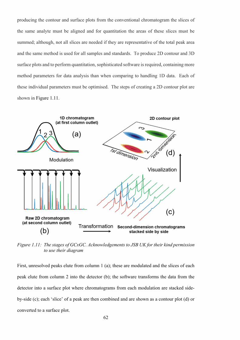
62

producing the contour and surface plots from the conventional chromatogram the slices of

the same analyte must be aligned and for quantitation the areas of these slices must be

summed; although, not all slices are needed if they are representative of the total peak area

and the same method is used for all samples and standards. To produce 2D contour and 3D

surface plots and to perform quantitation, sophisticated software is required, containing more

method parameters for data analysis than when comparing to handling 1D data. Each of

these individual parameters must be optimised. The steps of creating a 2D contour plot are

shown in Figure 1.11.

Figure 1.11: The stages of GCxGC. Acknowledgements to JSB UK for their kind permission

to use their diagram

First, unresolved peaks elute from column 1 (a); these are modulated and the slices of each

peak elute from column 2 into the detector (b); the software transforms the data from the

detector into a surface plot where chromatograms from each modulation are stacked side-

by-side (c); each ‘slice’ of a peak are then combined and are shown as a contour plot (d) or

converted to a surface plot.

63

1.3.3.6 Summary of GCxGC

GCxGC is very good for solving complex separation problems and is also good for

improving sensitivity, with very sharp peaks of approximately 30-40 ms wide, whereas

standard 1D GC produces peaks 2-3 seconds wide. However, thermally labile, active and

high molecular weight analytes can still be a problem. Matrix compounds can still cause

frequent maintenance of the instrument and enantiomers can still only be separated with the

use of a chiral column, therefore the sample preparation, sample introduction and detection

techniques must still be carefully selected and optimised.

1.3.4 Headspace (HS) analysis

1.3.4.1 Background to HS analysis

Headspace (HS) can be defined as the gas space above a sample when placed in a

chromatography vial and therefore HS analysis is the analysis of the analytes present within

that gas. Samples that can be analysed by HS analysis include anything that can fit in the

vial and release volatile compounds, these include liquids and solids. Usually, heat is applied

to the vial to assist in the release of the compounds. How much heat can be applied depends

on the boiling point of any solvent in the sample and the maximum temperature of the

instrument and the vial. For most HS analyses, it is always in the thermal desorption region,

below 350 °C, where carbon-carbon bonds are not broken.

1.3.4.2 Static HS

Static HS analysis takes place in a sealed vial. The sample plus any matrix modifier are

placed into the vial, which is then sealed with a septum and cap. Volatile analytes migrate

from the sample into the headspace and reach equilibrium, where the rate of analyte

molecules leaving the sample is equal to the rate of analyte molecules re-entering the sample.

64

A portion of the equilibrated headspace is then taken and injected into the GC for analysis.

Not all analytes are distributed equally between the sample phase and the gas-phase. The

equilibrium will depend on the volatility of the analyte, the temperature and matrix

properties and its affinity for the sample phase. The ratio of the analyte in the headspace to

the sample, under the chosen conditions, at equilibrium, is given by the partition coefficient

(K), where Cs is the concentration of the analyte in the sample phase and Cg is the

concentration of the analyte in the gas-phase:

= (1.8)

If K is large (>1) then analytes prefer the sample and a good recovery will not be obtained

in the analysis; if K is small (<1) then there is a higher concentration of analytes in the

headspace, resulting in a more sensitive analysis. For example, if the sample is hexane in

water, at 40 °C the partition coefficient is 0.14. A good recovery can be obtained, as the

hexane moves easily into the headspace as it is a non-polar analyte in a very polar

environment. Whereas, for methanol the partition coefficient is 1670, meaning that a very

low proportion of the analyte molecules will migrate into the headspace and be available for

analysis. Methanol is a very polar molecule in a very polar environment and as hydrogen

bonding is a very strong interaction it will keep the analyte molecules in the matrix, resulting

in an analysis with poor sensitivity.

There are several techniques to improve the detection limits of analytes with poor K values,

by increasing the concentration of the analytes in the headspace and thus lowering their K

values.

Raising the equilibration temperature reduces the solubility of analytes in the sample matrix

as well as reducing the time to reach equilibrium. For example, ethanol in water at 40 °C

has a K value of 1355, but at 80 °C the K value is reduced to 328, which would give a large

improvement in sensitivity (factor of ~4). The boiling point of the solvent should always be

65

considered, as a high concentration of solvent vapour in the headspace can reduce analyte

concentration in the gas-phase and affect the GC(-MS) separation and detection. For

example, the concentration of water vapour doubles with each 10 °C increase and therefore

an equilibration temperature of 60-80 °C is fine for most applications, but needs to be

optimised.

Another method of reducing the K values is to modify the matrix. The addition of salt to

aqueous samples decreases the analyte solubility by reducing hydrogen bonding. However,

there isn’t an equal effect on all analytes. The largest effect is on polar analytes with high K

values, but for those analytes with low K values it has little effect. There are several different

salts that can be used, including sodium chloride, sodium sulphate, sodium citrate,

ammonium chloride or sulphate and potassium carbonate. Which salt to use depends on the

properties of the analyte and the matrix. For example, in aqueous samples, at 60 °C, the

addition of ammonium chloride makes the ethanol peak area two times larger than with no

salt; whereas, the addition of potassium carbonate makes the peak area eight times larger

(PerkinElmer, Inc., 2014). The salt should not react with the sample or analytes, for example

sodium chloride reacts with brominated analytes, and it must be readily available with high

purity so as not to contaminate the sample.

Another example of matrix modification is changing the pH, which can minimise the

solubility of some analytes. Acidic analytes are more effectively extracted at acidic pH and

basic compounds are more effectively extracted at basic pH. For example, an acid present

in a sample at a basic pH with insufficient protons will dissociate into its conjugate base:

⇋ + (1.9)

The acidic analyte will become ionised, which makes it more polar, and therefore it will be

more difficult to move into the headspace in a polar environment. In an acidic sample, there

will be enough protons in solution for the acidic analyte to retain its proton, so it will be ion-

66

suppressed and remain in the neutral form. It is still polar in a polar environment, but less

polar than in its dissociated form. Partially ionised analytes do not have constant K values

and therefore the sample must be buffered to be either suitably acidic (pH 2-3) or basic (pH

8-9).

The addition of a co-solvent is a third matrix modification method used to enhance or

suppress the response of one analyte in comparison to another. For example, the addition of

dimethylformamide (DMF) to a water sample increases the recovery of acetonitrile, up to a

certain concentration. This is a useful method where there are only a few analytes that are

of interest, as it is difficult to find a co-solvent that only enhances and doesn’t suppress any

analytes of interest in the sample.

Analytes with reactive hydrogen atoms, such as acids, alcohols and amines can be

derivatised to improve their volatility, reactivity and solubility and thereby improve their K

values. For example, fatty acids (FAs) can be esterified in methanol with boron trifluoride

to become fatty acid methyl esters (FAMEs) or the acetylation of glycerol in acetic anhydride

with sodium carbonate. Derivatisation can be performed offline or automatically online,

using a GC autosampler as part of the HS analysis prior to analysis by GC.

After optimisation of the HS temperature and matrix modification, another parameter to

improve the sensitivity of the static HS method is to consider the phase ratio, β. β, is defined

as the relative volume of headspace (Vg) compared to the volume of sample (Vs) in the HS

vial: = (1.10)

Larger sample sizes result in lower β values and yield higher responses for volatile analytes,

however this is dependent on their K value. The impact of both β and K on the concentration

in the gas-phase, Cg, can be described by:

67

= ( ) (1.11)

The concentration of an analyte in the gas-phase is directly proportional to the initial

concentration (Co). If K is large then β is unimportant, the analyte molecules will stay in the

sample no matter what the phase ratio. If K is small, then β dominates and increasing the

amount of sample not only increases the concentration of analyte molecules in the headspace

but also the number of analyte molecules placed in the HS vial. Also, a larger proportion of

the headspace is removed for injection into the GC for analysis, overall resulting in a higher

concentration injected. Therefore, the key to a sensitive HS method is to obtain low K values

for all analytes by optimising the method and performing matrix modification.

Environmental and biological samples can contain variable amounts of salt and have variable

pH before any matrix modification is performed. Variable pH and salt content can have a

significant impact on the partition coefficient, partially ionised analytes don’t have constant

K values, therefore it is necessary to normalise samples to ensure consistency. It is relatively

easy to check the pH and adjust, but salt content is more difficult to determine, therefore it

is better to add salt to saturation. The volume of sample plus matrix modifier in the vial

must always be constant, to make sure β is reproducible, therefore care must be taken when

changing the pH to ensure a constant sample volume is maintained. These principles were

applied in Chapter 3.

1.3.4.3 The instrumentation available for static HS analysis

There are three types of instruments available to perform automated HS analysis into a GC:

• The gas-tight syringe instrument is an XYZ robot that uses an incubator to heat and

shake the HS vial for a given time and temperature. The heated syringe, which is at

a temperature higher than the sample to prevent condensation, takes an aliquot of the

headspace from the vial, moves to the GC inlet and injects the sample. Some sample

68

can be lost between the incubator and inlet due to pressure differences between the

vial and atmosphere. This loss can be reduced by minimising the syringe

temperature.

• The balanced pressure system heats the HS vial in a thermostatted oven before a

needle is inserted and the vial is pressurised with carrier gas. After equilibration, a

valve is switched for a fixed time, allowing the sample from the vial onto the column

through a heated transfer line. The total volume transferred is unknown.

• The pressurised loop system is similar to the balanced pressure system, however after

pressurisation the valve is turned and a loop of fixed volume is filled. The valve is

then turned again and the loop contents flushed onto the column with carrier gas

Both the valve systems have multiple connections with a complicated flow path that can

cause problems and can only be used for HS analysis. Whereas, in the gas tight syringe

system the sample pathway is very simple and the syringe can be changed to enable the XYZ

robot to perform other sample preparation and injection techniques, for example liquid

injection or SPME analysis.

Even with careful optimisation of the parameters, static HS is not a very sensitive technique,

as multiple dilutions occur between the sample and the column. Even with low K values,

not all the analyte molecules will be present in the headspace at equilibrium. In addition,

only a portion of the headspace is taken for injection, not the whole of it. Finally, the

headspace aliquot is injected under split conditions, to ensure a fast transfer to the column

and obtain narrow sample bands and therefore sharp peaks for the very volatile analytes.

This inevitably results in most of the sample making its way down the split-line and not

being available for analysis. As discussed in the following section, other techniques can

concentrate the headspace, where the analysis of species at trace level is necessary.

69

1.3.4.4 Dynamic HS

Dynamic HS takes place in a purged vial. A flow of carrier gas is purged over the sample

and continuously transfers the volatile analytes emerging from the sample to a trap, where

they are concentrated. Equilibrium is never reached and after a fixed period the purging

stops and the trap is thermally desorbed, to transfer the analytes to the GC column for

analysis. Alternatively, it can be eluted with an organic solvent for analysis using different

techniques. As most the analyte molecules are recovered, dynamic HS is more sensitive

than static HS, but only for those analytes with low partition coefficients. The sample is

treated in the same way as for static HS, with heating of the sample vial and matrix

modification to release the analytes from the sample matrix. This approach requires a further

step to be optimised. Namely, the selection of the optimal trap adsorbent(s) that both traps

and releases the analytes quantitatively with no break-through, irreversible adsorption or

catalytic breakdown, while providing the best recovery of the analytes. It is also

advantageous to choose a selective adsorbent that doesn’t trap the matrix, for example a

hydrophobic adsorbent for aqueous samples. The optimal adsorption and desorption

temperatures and flows must also be determined and care taken to minimise activity, dead

volumes and cold spots through the more complicated flow path and valve.

1.3.5 Solid-Phase MicroExtraction (SPME)

1.3.5.1 Background to SPME

Solid-phase microextraction (SPME) is a separation method that uses a solid phase to extract

analytes from a sample, based on their preferential affinity for the phase over the sample

matrix. It was developed in 1989, at the University of Waterloo, by R.P. Belardi and J.

Pawliszyn (Pawliszyn, 2011). It uses a fibre that is coated with a stationary phase that is

similar to the GC column stationary phase and can be a liquid polymer or a solid sorbent.

70

It can be used to extract and concentrate analytes from both liquid and gas-phase samples,

which includes the headspace above liquid and solid samples. The fibre is then inserted into

the GC inlet where it is thermally desorbed directly onto the analytical column, or it can be

desorbed with a liquid solvent, including within an HPLC interface. It is primarily a

solventless technique, therefore the vapour volume from a liquid injection and the solvent

vapour from a headspace injection are not problematic, if the correct fibre phase is selected

for the application. It can be a manual or an automated process and onsite sampling is

possible, if the fibres are appropriately stored for transport back to the laboratory. It is a fast

and simple technique for both rapid screening and quantitative analysis. For most methods,

it is recommended to use an IS for quantitation or semi-quantitation to reduce errors.

There is a linear relationship between the initial concentration of the analyte in the sample

and the amount adsorbed or absorbed by the fibre. The amount of analyte extracted is not

related to the sample volume, which means that the technique can be used for field sampling

in e.g. lakes, air, trees. VOCs require a thick phase, semi-volatile organic compounds

(SVOCs) and less-volatile analytes require a thin phase. By selecting the correct fibre,

analytes can be sampled with a precision of <12 % and certain analytes have parts-per-

trillion (ppt) detection limits. With headspace SPME (HS-SPME), any sample type can be

analysed that fits in a HS vial. With direct immersion SPME (DI-SPME), where the fibre is

inserted into the sample for extraction, the sample can be any liquid or slurry that is placed

into the HS vial and doesn’t damage the fibre when extracting.

1.3.5.2 Headspace-SPME

HS-SPME is more sensitive for volatile analytes that are predominantly in the headspace

above the sample. Prior to analyses, the fibre must be conditioned at the recommended

temperature and for the specified time for the phase type and thickness. The sample is pre-

shaken at high rpm and heated to establish an equilibrium between the sample and

71

headspace. The needle is then inserted into the vial and the fibre exposed to the sample

headspace while the vial continues to be heated and is shaken gently for 2-30 minutes to

concentrate the analytes onto the fibre phase.

The analytes form an equilibrium between the sample and headspace and between the

headspace and the fibre, respectively. It is a tri-phase system. As with HS analysis, the

release of the analytes into the headspace is improved with matrix modification, increasing

the temperature and by optimising the phase ratio. The fibre phase must be carefully selected

so that there is preferential affinity for it rather than the analytes returning to the sample at

equilibrium.

At the end of the extraction time, the fibre is retracted inside the needle, removed from the

sample vial and inserted directly into the hot GC inlet installed with a very narrow liner of

0.75 mm i.d. as it is a solventless injection and this also aids in a fast transfer onto the column.

The fibre is exposed and the analytes are quickly desorbed onto the column within 1-2

minutes.

1.3.5.3 Direct Immersion-SPME

DI-SPME is more sensitive for analytes predominantly in the liquid-phase. The fibre is

again pre-conditioned and the sample pre-shaken and heated. This time the needle is inserted

into the vial and the fibre exposed directly into the liquid sample to extract the analytes. The

analytes form an equilibrium between the liquid and fibre and between the liquid and

headspace. Unlike in HS analysis, there is no need for matrix modification, if there is

preferential affinity, through correct phase selection, for the fibre over the sample. The loss

of the analytes to the headspace is minimised by keeping the temperature low. Although, it

needs to be reproducible and therefore the lowest programmable temperature for the

instrument is set. Maximising the sample volume in the vial also minimises losses to the

headspace volume. After 2-30 minutes, depending on the application and the sample matrix,

72

the fibre and then the needle are retracted and quickly desorbed directly in the GC inlet. HS-

SPME keeps the fibre cleaner, minimises interferences and prolongs the life of the SPME

fibre versus DI-SPME.

For SPME, the distribution constant (Kfs) of the analyte between the fibre coating and the

sample is defined as:

= (1.12)

Where C∞s is the concentration in the sample at equilibrium, C∞f is the concentration on the

fibre at equilibrium, Vs is the volume of the sample and Vf is the volume of the fibre coating.

Nernst’s partition law for liquid polymeric coatings states that the mass of analyte absorbed

(n) by a single, homogenous liquid-phase coating at equilibrium where no headspace is

present is linearly proportional to the initial concentration (Co) in the sample, given as:

= = (1.13)

Where there is headspace present, the equation becomes:

= = (1.14)

The amount of an analyte extracted by the fibre coating doesn’t depend on the location of

the fibre, whether it is in the liquid-phase in DI-SPME or gas-phase in HS-SPME, if the

volumes of the two phases are the same in both sampling modes. Analytes can diffuse more

rapidly into the coating in HS-SPME than DI-SPME, with diffusion coefficients up to four

times higher in the gas-phase. Therefore, equilibrium is reached more rapidly in HS-SPME,

especially for volatile analytes that are already significantly in the headspace prior to

extraction.

73

1.3.5.4 The SPME fibre and coatings

The SPME fibre is 1-2 cm of fused silica bonded to a stainless-steel plunger or a length of

flexible metal alloy on which the phase is coated. The plunger is held within a needle which

is retracted to protect the fibre, especially when piercing a vial and the GC inlet septa. The

fibre is then exposed to extract the analytes from the headspace above or directly from the

sample. The phase coated onto the fibre can be non-bonded or bonded. Non-bonded fibres

are stable with some water-miscible organic solvents but swelling may occur and they can’t

be used with non-polar organic solvents. Bonded phases are more stable with all organic

solvents, although slight swelling with non-polar solvents is possible. The most stable

coating is cross-linked with bonding to the fibre core, these are stable in most solvents, with

slight swelling possible in some non-polar solvents.

The phase type and thickness are selected to absorb or adsorb the target analytes, the amount

of analyte extracted is dependent on the thickness of the phase and the partition coefficient

of the analyte. The SPME phase should be selected to match the chemistry of the analytes

to be extracted, i.e. their molecular weight (MW) and polarity. Unlike GC columns, small

changes in stationary phase polarity doesn’t give large selectivity differences, but the

addition of a sorbent onto a coating, for example strongly polar carbowax PEG onto a divinyl

benzene (DVB) polymer, increases the surface area and improves the extraction efficiency

of polar molecules.

Absorption describes the process of analytes dissolving into the coating or diffusing into the

bulk phase. The absorbent takes in the analytes in a non-competitive process and quantitative

analysis is usually unaffected by matrix composition. Absorptive fibres have a greater

capacity and broad linearity, as extraction is through partitioning of the analyte between the

two immiscible phases, e.g. the sample/liquid and the fibre/liquid-phase coating, which

could be PEG, PDMS or polyacrylate (PA).

74

Adsorption is the process of analytes interacting with the surface of a solid, usually through

physisorption, chemisorption or electrostatic attraction, depending on the analytes. The

analytes do not diffuse into the sorbent, unless there are pores. Adsorption is a competitive

process, as there are a limited number of surface sites, and the matrix composition and

extraction conditions affect the amount of analyte extracted by the fibre. Adsorptive-fibres,

such as Carboxen (CAR) and DVB, are better for extracting low concentration analytes,

Quantitation is linear only in narrow concentration ranges.

There are two main types of fibres: homogeneous pure polymer coatings or fibres with

porous particles embedded in the partially cross-linked polymeric phase. Homogeneous

pure polymer coatings, include PDMS, which is available in three different thicknesses to

match the volatility of the analytes, PEG and PA. Fibres with porous particles embedded in

the partially cross-linked polymeric phase have lower stability but high selectivity and are

usually a PDMS or PEG polymer with either Carboxen, DVB or a template resin porous

particles embedded. It is also possible for both DVB and CAR to be embedded in a PDMS

fibre. A fibre containing a mixture of different phases with different polarities benefits from:

a higher extraction selectivity, to increase recovery of specific analytes with a matched

polarity fibre; a reduced possibility of extracting interferences; enabling the extraction of

polar analytes from organic matrices.

Coating the fibre with a mixture of polymer and porous particles increases the porosity of

the fibre coating and hence its total capacity and its ability to retain analytes more tightly, as

well as increasing the pore size in the coating, thus increasing the analyte selectivity.

Thick phase coatings are selected to give higher sensitivity, as more molecules can be

extracted, or to retain VOCs without loss. However, the thicker phase has longer desorption

times for higher molecular weight (MW) analytes, carryover is also more likely to occur and

the phase bleeds more. Thin phase coatings ensure a faster diffusion and release of higher

75

MW analytes, have lower bleed but also results in lower sensitivity. The efficiency of the

analyte extraction and desorption from the fibre depends on several factors including: the

MW and size of analyte molecules; boiling point and vapour pressure of the analyte; polarity

and functional groups present in the analyte molecules and fibre phase(s); concentration in

the sample and the instrument used for separation and detection. Different fibres have

different operating temperatures and are conditioned for different lengths of time at different

conditioning temperatures, depending on the stability and thickness of the phase.

1.3.6 Thermal Desorption (TD)

1.3.6.1 Background to TD

Thermal desorption (TD) is a physical separation process, where heat is applied to a sample

to transfer analytes, that are adsorbed or absorbed in the sample, into the gas-phase so that

they can be analysed using gas chromatography. TD only uses temperatures up to 350 °C

and therefore no chemical bonds are broken in the process, only interactions. TD can be

used to analyse a range of species, from those as volatile as acetylene (with two carbon

atoms) up to molecules with forty carbons, such as polyaromatic hydrocarbons (PAHs) and

phthalates.

Small solid or viscous liquid samples can be directly thermally desorbed by placing in a

conditioned TD tube. Gas-phase analytes can be concentrated by drawing the gas-phase

sample through a conditioned TD tube packed with a sorbent. For example, parts-per-trillion

(ppt) levels of PAHs can be detected in air analysis, by drawing 100 L of air through a packed

TD tube.

After placing the sample in the tube, or concentrating the gas-phase sample in a packed tube,

the tube is placed in the TD instrument and leak checked. On passing, it is pre-purged with

76

carrier gas, usually helium, to remove atmospheric oxygen and to prevent oxidation of the

sample on heating. The TD tube is then heated to a temperature dependent on the maximum

temperature of the sorbent, the volatility of the analytes and the nature of the sample. It is

then held at that temperature, for usually 5-30 minutes, to fully desorb the sample or sorbent.

The TD tube is continuously purged while heated and the emerging analytes are back-flushed

off the TD tube and selectively concentrated on a narrow cold trap, containing a small

amount of sorbent. During this process, unwanted gases, water and matrix are removed. If

the sample is very concentrated, the analytes can be transferred to the cold trap in split, rather

than the usual splitless mode. After the TD tube is fully desorbed, the cold trap is rapidly

heated and the concentrated analytes are back-flushed through a heated transfer line, usually

as a split injection, onto the GC analytical column in a narrow sample band for separation

and detection.

1.3.6.2 Sampling for TD analyses

Gas-phase samples can be sampled in-situ by drawing the sample through a conditioned,

packed TD tube using a constant pressure or constant flow pump. The tube is then sealed,

to prevent the loss of analytes and the ingress of contaminants, and returned to the lab for

analysis. Tubes can be stable for several weeks.

Passive sampling is frequently used for occupational hygiene to monitor indoor and ambient

air, by using a packed TD tube with an axial diffusive sampler to enable exposure of the tube

sorbent to the sample. Radial diffusive samplers, after sampling, can also be analysed by

TD-GC by placing them in an empty TD tube for analysis.

On-line instruments continuously pump the sample directly onto a pair of cold traps,

switching between collection and analysis as frequently as required. No TD tubes are

required for this mode of operation.

77

Gas-phase samples can also be sub-sampled by filling Tedlar, Teflon, polyvinyl chloride

(PVC), charcoal-filled or multi-layer foil bags, or canisters, with the sample. Which type of

container is used depends on the nature of the sample and the field site. It is important to

ensure that the container has low permeability and has high inertness to the sample. It must

be leak-tight and shouldn’t be damaged in the sampling location, to ensure analytes do not

become stuck or lost. The container should also not contaminate the sample.

1.3.6.3 Important parameters for TD analyses

Before use, TD tubes must be conditioned and sealed before taking to the sampling location.

Those packed with a sorbent, must be conditioned at the optimal temperature for the required

time for the specific sorbent(s) used.

The break-through volume for the samples and analytes to be sampled must be determined

before sample collection, so that a known volume of sampled gas can be taken that is below

the break-through volume. Break-through volume can simply be checked for by attaching

two sampling tubes in series; if the first tube becomes saturated any analytes breaking-

through will be trapped by the second tube, this can then be analysed to determine if the

break-through volume has been exceeded.

When sampling, the optimal flow rate through the tube affects the interaction of the analyte

with the sorbent and therefore the amount that can be trapped. The optimal sampling rate

through a standard 5 mm i.d. packed TD tube is 50 mL/min, with a working range of 10-200

mL/min which can increase to 500 mL/min for a maximum of 10 to 15 minutes. Sample

volumes range from 500 mL to 100 L.

There are improved adsorption efficiencies at lower temperatures, however the ambient

temperature during sampling must be considered when selecting the sorbent(s). Where there

is a wide range of analyte physical and chemical properties, a tube can be packed with

78

multiple sorbent beds, usually up to three, so that there can still be enough mass of each

sorbent for the capacity required. The weakest sorbent is packed closest to the sample, with

the strongest sorbent packed furthest from the sampling end of the tube to enable the fast

and efficient release of the analytes in the reverse direction. The analytes are back-flushed

to the next stage of the TD process.

Where replicate sample aliquots are required, a manifold sampling system can be used where

there are multiple tubes, either containing the same sorbent(s) for repeatability checks or

containing different sorbents to sample for different analytes. These are set-up in parallel

and are all connected to the same pump, but with flow control valves for each, to either

balance the flows or to set individual flows for each TD tube.

1.3.6.4 TD Tubes

The TD tube itself can be made from: glass, which is good to see the position of samples

placed directly into the tube; stainless steel which makes it very robust, especially for those

tubes sampled away from the lab; or coated (silco) steel, which makes the tube very inert

and is much better for active analytes such as those molecules containing sulphur.

The tubes vary in size depending on the manufacturer, but the industry standard TD methods,

such as ISO, CEN, ASTM and EPA, use 3.5 inch x ¼ inch outside diameter (o.d.) tubes.

Tubes should have a unique identifier, which enables the sample to be matched to the tube

and the sampling direction must be known so the tube is desorbed in the reverse direction to

ensure that all the sampled analytes are recovered.

1.3.6.5 Sorbents for TD

Similar to SPME, the sorbents placed into the TD tube and the cold trap can either interact

with the analytes through absorption or adsorption. The sorbent(s) selected is dependent on

the target analytes. It must trap the target analytes at the ambient temperature of the sampling

79

location and easily release them again when rapidly heated. This temperature must be no

higher than the maximum temperature of the sorbent, with no irreversible ad/absorption or

catalytic breakdown.

Common sorbents are polymers such as Tenax ®, Porapak, Hayesep or Chromosorb, a styrene

DVB polymer; carbon molecular sieves such as Sulficarb, Carbosieve or Carboxen; zeolite

molecular sieves; graphitised carbon black such as Carbopack, Carbotrap or Carbograph.

Tenax® and graphitised carbon blacks are hydrophobic and therefore good for ‘wet’ samples.

Carbon molecular sieves are mostly hydrophilic with Carboxen being the most hydrophobic.

Zeolite molecular sieves are very hydrophilic and can collect water up to mg levels, in a

typically sized TD tube.

Different types of sorbents are good for different volatilities and polarities of analytes and

have different retention volumes and maximum temperatures (ranging from 190-400 °C).

Even when the maximum temperatures are not exceeded, some sorbents can produce

artefacts – the release of molecules, that are focused, separated and detected by GC. Carbon

molecular sieves have minimal artefact levels, whereas Tenax® has a low artefact level when

new; however, as the sorbent ages the artefact level increases.

Porous polymers and carbonised molecular sieves are more inert than graphitised carbon

blacks such as Carbograph 1TD. Generally, the more volatile the analyte(s), the stronger the

sorbent must be. For analytes with a boiling point (bp) > 100 °C a weak sorbent such as

Tenax® TA is used. Those analytes with a boiling point of between 30-100 °C require the

use of a medium strength sorbent such as Carbograph 1TD and very volatile analytes with a

boiling point between 30-50 °C require the of use a strong sorbent such as Sulficarb or

Carboxen 1000.

80

The mesh size of the packing material affects the packing density and the back pressure that

it creates. A mesh size of 20/40 has larger particles than 60/80 and therefore can be sampled

using higher flow rates.

The sorbent life of the tube is dependent on the type of sorbent(s) used, the maximum and

routine desorption temperatures it has been exposed to and the number of desorption cycles,

which includes conditioning of the tubes. Tenax® and carbon-based sorbents are usually

good for 100-200 cycles, whereas porous polymers are less stable, usually with a life of 100

cycles.

A trap is used to collect and focus analytes between the TD tube and the GC analytical

column. Without it, the long TD tube desorption times would result in long transfer times to

the column, producing broad sample bands and poor chromatographic resolution and peak

shapes. The analytes can be trapped through cryofocusing in the inlet liner or on a GC pre-

column using cryogens or through cold trapping with a Peltier cooled trap (cold trap). The

cold trap enables the use of a small amount of sorbent in a narrow tube to selectively

concentrate the analytes, but unlike the TD tube, the cold trap is cooled below ambient

reducing the likelihood of breakthrough even though less sorbent is used. With

cryofocusing, everything released from the TD tube is trapped, but with the cold trap the

sorbent can be selected to not trap unwanted gases such as water, solvents, etc. Like with

the TD tube sorbent, it must trap the target analytes at the (lower) temperature chosen and

then easily release them with no catalytic breakdown when the trap is rapidly heated. As the

cold trap is backflushed, multiple sorbents can be chosen, usually up to three, to match the

target analytes. On rapidly heating the narrow cold trap, the analytes are usually transferred

to the GC column in split mode to increase the flow through the cold trap when desorbing,

resulting in a faster transfer to the GC column and therefore a narrow sample band. Even

with a low split ratio, the sample flow to waste is higher than that onto the column. More

recent instrumentation can automatically enable the split flow effluent from the cold trap

81

desorption to pass back through the original sample TD tube or through a new, conditioned

TD tube to re-collect the sample. This means that TD samples are no longer one-shot, where

if something went wrong with the analysis of that sample it could not be re-analysed. In

addition, the recovery is quantitative, therefore if the sample does have to be re-analysed the

original concentration can be determined based on the split ratio. Sample re-collection can

also be achieved through the trapping of the split effluent from the TD tube desorption onto

a new, conditioned TD tube if a split method was used.

Quantitation can be performed, as in other techniques, by analysing the standards using the

same method as the samples. A maximum of 1-2 µL of standard solution, preferably in a

solvent that is not trapped by the sorbent and has a low vapour expansion coefficient, or its

headspace is directly spiked onto the TD tube using a spiking rig. The rig enables the

standard to be injected into a carrier gas so that the analytes are blown through the TD tube

sorbent and then any solvent is purged before analysis. The automatic addition of IS to the

TD tube and/or the cold trap is possible and is instrument dependent.

1.3.7 Bioinformatics and Chemometrics

Analytical techniques, such as GC-MS, can generate large volumes of information and can

be thought of as a method of data generation and collection. Several chromatograms can

manually be compared to identify patterns, but multiple complex chromatograms or

hundreds of simple chromatograms can be far more difficult. The processing of large data

sets of complex chromatograms can take as long as, if not even longer than the sample

analyses. This can happen, especially, when making sense of and trying to find the answer

to the question(s) asked, when there are many variables generated for each sample and large

numbers of samples analysed. There are multiple steps to the processing of that data,

including data preparation or pre-processing, extraction of the information, processing of the

information, interpretation and then reporting of the result. It is very important to both

82

design and evaluate experiments, there are multiple different techniques used to validate

results throughout the process (Broadhurst & Kell, 2006).

1.3.7.1 Bioinformatics and cheminformatics

Bioinformatics and cheminformatics are general terms that describe the use of computer

programming as part of the methodology in the analysis of biological or chemical data. They

develop methods and software tools using computer science, mathematics, statistics and

engineering to process, analyse and interpret the data that can come from a variety of sources,

not just for one-off investigations but also in routine analysis. Bioinformatics uses

computation to better understand biology by analysing biological data rather than building

theoretical models of biological systems and therefore relies on the generation of sometimes

large amounts of high quality data. This data is inputted to the computer system that uses

algorithms generated from artificial intelligence and data mining that depend on discrete

mathematics and statistics to process that data. Originally, bioinformatics was invented by

Paulien Hogeweg and Ben Hesper in 1970 to describe the study of information processes in

biotic systems parallel to the biophysics field and biochemistry. Today, bioinformatics is

used in many areas of biology, including molecular biology, genetics and genomics.

Bioinformatics can use a variety of techniques to understand the biological processes and is

mostly involved in the study of genes and large proteins, whereas cheminformatics has its

roots in chemometrics, chemical information and computational chemistry focusing on the

study of small molecules.

1.3.7.2 Data mining

Data mining, otherwise known as knowledge discovery, is a sub-field of computer science

that appeared around 1990. It is the automatic or semi-automatic analysis of large data sets

to discover previously unknown patterns of interest, the extraction of the information and

83

the presentation of it for further use, for example in machine learning. Data mining methods

and tasks can be artificial neural networks (ANN), support vector machines (SVM), outlier

detection, association rule learning to discover interesting relationships between variables,

cluster analysis and classification, regression to find a model with the least error and

summarisation.

1.3.7.3 Machine learning

Machine learning is also a sub-field of computer science that enables the computer to learn

without being explicitly programmed, by using algorithms that can learn from and make

predictions with the data. The algorithm builds a model with the data that it is given and

uses this to make the predictions or decisions. The accuracy of these are very dependent on

both the quality and the quantity of the data that is used to generate the model, plus the

testing of the hypothesis. The algorithms used can be very complex, generating very

complex models which can then be used to produce reliable, repeatable decisions and results.

1.3.7.4 Artificial Neural Networks (ANN) and Probabilistic Neural

Networks (PNN)

Artificial neural networks (ANN) were created to process information and there are a wide

variety of ANNs to model, for example, behaviour and control in animals and machines, but

they are also used in pattern recognition, forecasting and data compression. They were

inspired by the human central nervous system and are used in machine learning to describe

relationships in a network of variables where there are many, usually unknown inputs which

the estimated functions depend on. The architecture of the ANN is similar to a neural

network, an interconnected group of nodes (neurons) that specify the variables involved in

the network and their relationships. For each neuron, there are large number of inputs, these

are similar to synapses, which are multiplied by weights, for example the strength of the

84

respective signals, and then a mathematical function is applied to determine the activation

of the neuron or to compute the output. The weights can be adjusted to obtain the output

that is wanted for the specific inputs. The higher the weight the stronger the input, or a signal

can be inhibited by a negative weight. An ANN can have hundreds to thousands of neurons,

the activities of which will affect each other, therefore algorithms are required to adjust the

different weights to obtain the desired total output.

Probablistic neural networks (PNNs) are used for classification and they are much faster to

train. The radial base layer makes PNNs different to other networks, which calculates the

distances between the input vectors and the input weights. If these are very close together

the output is 1. All outputs are then summed to attain a vector of probabilities. A competitive

layer is then applied where the maximum of the probabilities is selected to produce a total

of 1 for a target class and 0 for all others.

1.3.7.5 Support Vector Machines (SVM)

Support vector machines (SVM) are used for classification and regression analysis by

constructing a hyperplane, or set of hyperplanes, in a high or infinite dimensional space.

However, they are only directly applicable for two-class tasks rather than multi-class. They

are supervised learning models that can use a SVM training algorithm to build a model based

on a given set of labelled training data with, for example, assigned classifications. The

classifications are then mapped in the space, as far apart as possible. When new samples are

mapped into the same space they can then be correctly classified. Unlabelled data cannot be

modelled with supervised learning by SVMs. Unsupervised learning, called support vector

clustering, attempts to find natural clustering within the data, it splits them into groups and

maps them in the space, which can then be used to map and classify new, unknown data.

There are multiple different types of SVM kernels, the linear (SVM-LIN) and radial basis

function (SVM-RBF) kernels were used in this thesis.

85

1.3.7.6 Random forests (RFs)

In machine learning, the random forests or random decision forests algorithm uses many

uncorrelated decision trees for the training in regression, classification and other

bioinformatics tasks. These are used to combine learning models and output the mode (most

frequent value) in classification or the mean prediction in regression to increase the accuracy

of the classification or prediction by averaging noisy and unbiased models to create a model

with low variance and that doesn’t overfit the training set.

1.3.7.7 Pattern recognition

Pattern recognition focuses on the similarities – patterns and regularities - in the data and is

a branch of machine learning. Supervised learning is when labelled ‘training’ data is used

in the machine learning, for example if the data from ‘good’ samples and ‘bad’ samples is

used to generate the model. This model can then be used to classify if an unknown sample

is statistically ‘good’ or ‘bad’. Unsupervised learning is when there is no labelled data and

therefore other algorithms must be used to discover previously unknown patterns in the data.

Semi-supervised learning is when there is a combination of labelled and unlabelled data.

All models created must be tested and therefore the data is usually split into a training set

and a test set. Once a model has been created with the training set, the test set can then be

used to test the model and check for model error, this is called cross-validation. Overfitting

happens where the statistical model describes the random error or noise, rather than the

underlying relationships and can occur where there are far too many parameters relative to

the number of samples, resulting in a very complex model that has poor predictive

performance and exaggerates the minor differences in the training data. By testing the model

on unused data, these exaggerations can be ruled out, a different selection of training data

and test data can be chosen from the data set, a new model created and tested. Multiple

rounds of cross-validation are performed to reduce variability and the validation results are

86

averaged. With very large data sets, the data can be partitioned with usually 70 % for training

and 30 % for testing, however for smaller data sets cross-validation is better as it ensures

enough data for significant modelling and testing.

1.3.7.8 Cluster analysis

Cluster analysis is the organisation of samples into groups that are more similar to each other

than other samples in different groups, it is also known as unsupervised classification. It is

a significant task in data mining and is used in machine learning and pattern recognition.

Cluster analysis isn’t a single algorithm, there are many algorithms that could be used. The

cluster models presented in the data depend on the algorithm used to define a cluster and

how it finds them. Cluster models include models based on distance connectivity such as

hierarchical cluster analysis (HCA); centroid models where a cluster is represented as a

single mean vector; distribution and density models; subspace and group models; and graph-

based models. Clustering can be ‘hard’, where each sample either belongs to a cluster or

not; or ‘soft’, where the sample belongs to each cluster by a certain degree. Clusters may

have: strict partitioning, where each sample belongs to one cluster; overlapping clustering,

where samples may belong to more than one cluster; hierarchical clustering, where samples

belonging to a child cluster also belong to a parent cluster; or subspace clustering, where

samples are not expected to overlap in a uniquely defined subspace, even though there is

overlapping clustering. Outliers are those samples that do not belong to any cluster. Cluster

analysis isn’t an automatic task, as the algorithm chosen or algorithm’s parameters may need

to be changed or the data pre-processing or model parameters modified to obtain the optimal

result.

87

1.3.7.9 Multivariate statistics

Multivariate statistics is the simultaneous analysis of more than one statistical outcome

variable and has always been a large part of chemometrics, as the data from these analytical

techniques is multivariate with potentially thousands of data points per sample. Multivariate

techniques construct a mathematical model that relates the multivariate data to the sample.

There are different approaches in the analysis of the data - those which are good at describing

the measured analytical response, known as the classical methods, or those that are good at

predicting the property of interest, known as the inverse methods.

1.3.7.10 Principal Component Analysis (PCA)

Principal component analysis (PCA) was invented in 1901 by Karl Pearson. It reduces the

number of dimensions of a data set, the predictive variables, by building a new set of co-

ordinates known as principal components (PC). The number of PCs cannot exceed the

number of variables or samples, whichever is smaller. PCs are linear combinations of the

original variables which are orthogonal to each other and therefore uncorrelated, which can

be used to summarise the data without loss of too much information. The first principal

component, PC1, accounts for the greatest amount of variability within a data set. PC2

accounts for the second largest amount of variability and is orthogonal to PC1, and so on for

PC3, PC4, etc. PCA analysis is mostly used in exploratory data analysis and for making

predictive models to identify outliers, determine patterns of association – natural groups

(clusters) within a data set and to determine variability. The results of PCA analysis can be

visualised with a scatterplot, for example a two-dimensional scatter for PC1 vs. PC2, or a

three-dimensional scatter plot for PC1 vs. PC2 vs. PC3 in which it is easy to see clusters of

data, if they are present. PCA is an unsupervised dimension reduction method that doesn’t

consider the correlation between the dependent and independent variables. It is the most

widely used multivariate statistical technique (Brereton, 2007).

88

1.3.7.11 Regression and Partial Least Squares Discriminant Analysis

(PLS-DA)

Statistical regression analysis is a generic name for all methods that attempt to fit a model to

observed data so that a relationship between two groups of variables can be quantified. This

model can then be used to describe their relationship or predict new values. The two data

matrices are usually denoted X and Y, regression attempts to build a model Y = f(X) to

explain or predict variations in the dependent variable(s) Y, from variations in the

independent variable(s) X, by applying the function f. Univariate data has a single predictor

X, whereas multiple linear regression (MLR) simultaneously considers multiple predictive

X variables resulting in a more accurate model.

Partial least squares (PLS) Regression combines the output from PCA with multiple

regression and is particularly useful when multiple dependent variables need to be predicted

from a very large set of independent variables. PLS is a supervised dimension reduction

method as it looks at the correlation between the dependent and independent variables and

unlike PCA, all variance in the data is explained and it is considered to be better at explaining

complex relationships (Maitra & Yan, 2008). PLS is good when there are more predictor

variables than observations and when there are multiple predictor variables with high

correlation, meaning that one can be correctly predicted from the others.

Partial least squares-discriminant analysis (PLS-DA) (Barker & Rayens, 2003) replaces the

dependent variable with a categorical one that describes the cluster. The clusters are already

known and therefore PLS-DA is used to determine if the clusters are actually different and

what features best describe the differences between the groups. It can improve the resolution

between clusters by rotating the PCA components to obtain maximum separation between

the classes and determine the variables that can separate those classes. This is particularly

useful in analytical chemistry to identify the experimental variables that contribute to the

89

difference. However, PLS-DA is prone to overfitting the data and therefore must be properly

validated (Westerhuis, et al., 2008).

The key information that can be gained from PLS-DA are the scores and weights of the

model. The score describes the position of each sample in each determined component,

otherwise known as a latent variable (LV). Latent variables are not observed but are shared

variance from other variables that are directly measured and that can be grouped together in

a model representing an underlying hypothesis, they are good at reducing the dimensionality

of the data. The most important information or characteristics should typically be held in a

low number of LVs, such as important chromatographic peaks, for example in LVs 1-4. The

less important information, such as noise, is held in the higher LVs, for example in greater

than 20 LVs. The weights describe the contribution of each variable to each LV. The PLS

loadings plot enables visualisation of the most significant features of the sample data file

from the PLS-DA.

1.3.7.12 Hierarchical Cluster Analysis (HCA)

Hierarchical cluster analysis (HCA) is also an exploratory algorithm that is used to assure

the validity of raw data by finding outliers and to show clusters of data. It arranges the

network into a hierarchy of groups, usually a dendrogram is produced that shows the

hierarchy of the individual samples and clusters those samples according to their similarities.

Agglomerative HCA starts at the bottom in a cluster and then pairs of clusters are merged

while moving up the hierarchy. Divisive HCA starts in the cluster of all samples and then

the clusters are split while moving down the hierarchy. The splitting or combining of clusters

relies on a measure of dissimilarity between the samples, usually in HCA this is the

connectivity distance.

90

1.3.7.13 Correlation Optimised Warping (COW)

There are multiple methods for data alignment, including dynamic time warping (DTW),

local warping and parametric time warping (PTW). Correlation optimised warping (COW)

(Tomasi, et al., 2004) is the preferred route for aligning data from analytical instruments that

has suffered drift, such as shifts in retention time, as it preserves the peak shape and area.

One data file is chosen to be the reference and is used to align the whole data set. The

reference data file and the sample data file are both divided into segments. Each segment of

the sample data file is then compressed or extended compared with interpolation and

converged to the reference data file. The two parameters optimised in this procedure are the

segment length (the number of data points in each segment), and the slack size (the number

of data points that can move between the segment boundaries). The parameters can be

selected using an automated method to compute a ‘simplicity’ value for each segment and

slack parameter combination for a discrete number of chromatograms. This is used to

measure how accurately those chromatograms are aligned. The best combination can then

be used to align the full data set using the optimal parameters.

1.3.7.14 Data Scaling

Data within a data set can be scaled to normalise the range of independent variables or

features. For example, with GC-MS data the abundance can be normalised against the

internal standard. Several different methods (and therefore equations) can be used for

scaling, including auto-scaling, mean-centring, range scaling between 0 and 1 and range-

scaling between -1 and +1 (Otto, 2007).

1.3.7.15 Feature selection and t-tests

Feature selection is a filter method that selects the variables that are most distinctive for each

class of samples or deselecting the features that are not at all significant. It is a crucial step

91

before sending data to a classifier algorithm, so that only the most significant data is sent

and therefore a higher classification accuracy can be achieved. A decision rule is applied to

decide if two variables belong to the same population (Glantz, 2005) or not. The Student t-

test tests the hypothesis about the mean of a small sample drawn from a normally distributed

population, when the population standard deviation is unknown. The Wilcoxon test is non-

parametric, meaning that it doesn’t assume the data is normally distributed.

1.3.7.16 Cross-Validation, Leave-One-Out Cross-Validation (LOO-CV)

Cross-validation, otherwise known as rotation estimation is a way of validating a model to

estimate how accurately a predictive model performs in practice. When an algorithm is

trained with a training dataset it is then usually tested with a testing data set. Cross-

validation, defines a validation dataset to test the model while it is being trained, to minimise

problems such as overfitting of the data and to see how the model will generalise to

unknown, real data.

Leave-one-out cross-validation (LOO-CV) (Hastie, et al., 2009) uses one sample as the

validation set and the remaining samples for the training set. For a dataset of n samples the

learning and validating process then occurs n times to classify 1 sample against a model built

using n-1 samples and therefore n models are built. Data is then produced about the true

positive rate (if the 1 validation sample is positive and is predicted as positive in the

validation) and the true negative rate (if the 1 validation sample is negative and is predicted

as negative in the validation).

Where there are very large data sets, leave-five-out cross-validation (LFO-CV) may also be

used to speed up the validation process.

92

1.3.7.17 Bootstrapping or resampling methods

Bootstrapping is a resampling technique that is good at determining accuracy, for example

variance, bias, confidence intervals or prediction error. It is a test or metric that relies on

random sampling with replacement, where it selects a subset from the dataset or statistical

population, called the resample or bootstrap sample, to estimate characteristics of the whole

population. As the randomly selected sample is replaced before the next random sample is

selected, it is probable that at least one sample is reselected. The process is repeated many

times and, for each subset generated, the standard errors can be calculated.

1.3.7.18 Monte Carlo simulation and null hypothesis model

A Monte Carlo simulation (Brereton, 2009) carries out repeated random sampling by

assigning a random class (in this work, disease positive or disease negative) to each sample,

generating many data sets, each is then used to produce a null model. The null model is

generated from a set of data that is statistically similar, but from which a meaningful

classification model is not expected. For a disease discriminant model using the real sample

classes to be considered significant, it must achieve a classification accuracy far higher than

that produced by the null models.

1.3.7.19 Sensitivity & specificity

When evaluating clinical data, the sensitivity and the specificity are calculated and reported

for the test (Lalkhen & McCluskey, 2008). These values are independent of the population,

the defined groups of patients, and do not consider the cut-off point for a particular test.

To calculate the sensitivity and specificity, the following must be determined:

• Number of true positives (TP): those patients with the disease and the test results in

a positive outcome.

93

• Number of true negatives (TN): those patients who do not have the disease and the

test results in a negative outcome.

• Number of false positives (FP): those patients who do not have the disease but the

test results in a positive outcome.

• Number of false negatives (FN): those patients with the disease but the test results in

a negative outcome.

Sensitivity is defined as the ability of the test to accurately identify patients with the disease: (%) = 100 (1.15)

A sensitivity of 100 % means that all patients with the disease were correctly identified. A

sensitivity of 75 % means that 75 % of the diseased patients were correctly identified as

positive. However, 25 % of the diseased patients were not identified as having the disease,

resulting as false negatives. A high sensitivity test result means that patients that have or

might have the disease will be identified for further tests and it is unlikely that patients with

the disease will be incorrectly identified as being negative.

Specificity is defined as the ability of the test to accurately identify patients who do not have

the disease: (%) = 100 (1.16)

A specificity of 100 % means that all patients without the disease were correctly identified.

A specificity of 75 % means that 75 % of the non-diseased patients were correctly identified

as negative. However, 25 % of the non-diseased patients were identified as possibly having

the disease, resulting as false positives. A low specificity test results in many patients that

do not have the disease being identified as possibly having it. This results in further worry

and discomfort for the patient who is then sent for further tests at more expense, when they

do not have the disease.

94

A test with high sensitivity and low specificity results in few patients with the disease being

mis-diagnosed, but many disease-free patients being sent for unnecessary further tests. With

a high cut-off point, there are fewer FPs but more FNs resulting in a highly specific but not

very sensitive test. With a low cut-off point, there are less FNs but more FPs resulting in a

highly sensitive but not very specific test.

1.3.7.20 Overall classification

It is useful to know the overall number of samples that are correctly classified (CC) either as

TP or TN with a model: (%) = 100 (1.17)

If the sensitivity and the specificity values are similar, then the overall classification will

give a similar, mean value. If sensitivity is low and specificity is high, or vice versa, the

overall classification is higher than the average of the two values.

1.3.7.21 Positive Predictive Value (PPV) and Negative Predictive Value

(NPV)

The positive predictive value (PPV) is useful for judging the likelihood that the patient has

the disease if the test result is positive: (%) = 100 (1.18)

The negative predictive value (NPV) is useful for judging the likelihood that the patient does

not have the disease if the test result is negative:

(%) = 100 (1.19)

The higher the PPV or NPV, the more believable the result. However, both the PPV and

NPV are also dependent on the prevalence of the disease in the population. If the population

has equal numbers of diseased and non-diseased patients and the sensitivity and specificity

95

are very high, the PPV is very high. If the number of diseased patients is low compared to

the number of non-diseased patients, then the PPV falls. Therefore, the prevalence of the

disease in the population must also be considered when examining PPV and NPV values.

1.3.7.22 False Discovery Rate (FDR)

The false discovery rate was formally described by Yoav Benjamini and Yosi Hochberg in

1995. It is used when conducting multiple comparisons to hypothesise the rate of false

positives in null hypothesis testing. This is important to check that significant features are

not rejected in any filter methods such as feature selection using the Wilcoxon test

(Motulsky, 2010).

The FDR is a measure of the overall number of diseased samples that have been incorrectly

classified as diseased (FPs) out of all samples that have been classified as diseased:

(%) = 100 = 100 − (%) (1.20)

1.3.7.23 Area Under Receiver Operating Characteristic (AUROC)

Receiver operator characteristic (ROC) curves were originally produced by radio receiver

operators to determine the reason why US radar had failed to detect the Japanese aircraft

after the attack on Pearl Harbour (Ekelund, 2012).

The receiver operating characteristic is a graphical plot of true positive rate (TPR) against

false positive rate (FPR) at various threshold settings, that is used to illustrate the

performance of a classifier, as shown in Figure 1.12.

It is used to determine the best cut-off for a test, with the highest TPR and lowest FPR. The

TPR is the equivalent of sensitivity and FPR is calculated as (1 – specificity). The area under

96

the receiver operating characteristic (AUROC) curve measures the test’s discriminative

ability.

Figure 1.12: Receiver Operator Curves (ROC) showing AUROC values and significance

When using normalised units, the AUROC curve is equal to the probability that a classifier

will rank a randomly chosen positive instance higher than a randomly chosen negative one.

It is equivalent to the Wilcoxon signed-rank test.

The AUROC curve can be calculated using the trapezoid rule, meaning the region under the

graph is approximated using the equation for a trapezoid.

97

A perfect test results in an AUROC value of 1.0. Whereas, a test that is not at all useful

results in an AUROC value of 0.5, meaning the test is as likely to produce the correct result

as flipping a coin, see Table 1-3.

Table 1-3: Significance of AUROC values for receiver operator characteristic curves

Category Fail Poor Fair Good Very good

AUROC 0.5-0.6 0.6-0.7 0.7-0.8 0.8-0.9 0.9-1.0

1.4 Thesis Overview

All analyses were performed at the School of Physical Sciences, (formerly Planetary and

Space Sciences Research Institute (PSSRI) in the Faculty of STEM), at The Open University.

Prior to the work reported in this thesis, there was no tradition of utilisation of GC-MS for

medical diagnostics.

The foregoing chapters describe a journey from the initial challenges of developing the

methods to a solution which combines the selectivity of a HS-SPME and the separation

capabilities of GC-ToFMS. The optimised method will be evaluated for its suitability for

detecting patients with bladder cancer, prostate cancer and hepatic disorders. Separate

methods were developed for the identification of the causative agents of sepsis, from the

profile of the volatile compounds present in the headspace above culture samples.

Chapter 2: Outlines the optimised experimental methods, the chemicals and reagents, the

instrumentation and the preparative procedures used for clinical studies reported in this

thesis.

Chapter 3: Summarises the development of the optimised methods reported in Chapter 2.

The extraction methods and instrument operating conditions have been developed by a

98

mixture of experience, critical review of published literature, personal communications and

a degree of trial and error.

Chapter 4: The optimised HS-SPME-GC-ToFMS method developed in Chapter 3 and

reported in Chapter 2 was applied to the study of a cohort of urine samples collected from

patients with bladder cancer or controls.

Chapter 5: The optimised method HS-SPME-GC-ToFMS developed in Chapter 3 and

reported in Chapter 2 was then applied to the study of a cohort of urine samples collected

from patients with prostate cancer. A mathematical model was then developed to determine

if the cancer positive samples could be distinguished from those from patients with benign

prostate hyperplasia (BPH) and controls.

Chapter 6: The optimised HS-SPME-GC-ToFMS method developed in Chapter 3 and

reported in Chapter 2 was also applied to the study of a cohort of urine samples collected

from patients with hepatic disorders. A model was then developed to determine if the

samples could be distinguished from those controls.

Chapter 7: Reports on a pilot study that utilised the HS-GC-MS and HS-TD-GC-MS method

reported in Section 2.3. The method was applied to the study of the profile of volatile organic

compound present in the headspace above a range of bacteria that are known to cause sepsis.

A model was then developed to determine if the bacteria samples could be distinguished

from each other and from controls.

Chapter 8: Conclusions and future work

99

Experimental

100

2.1 Introduction

This chapter is divided into three sections, based on the individual studies conducted within

this thesis and the methodologies used. Section 2.2 summarises the optimised methods

applied to the analysis of the headspace of clinically relevant urine samples by SPME,

followed by analysis by GC-MS (SPME-GC-MS). The section is organised to provide a full

description of materials and equipment used in each study, any sample handling or

preparative methods applied and the instrumental settings used. This section is the basis of

the studies on clinical samples reported and discussed in Chapters 4, 5 and 6, respectively.

It should be noted that it is Chapter 3, the Method Development chapter, which summarises

how the parameters reported in this chapter were initially conceived, developed and

optimised.

Section 2.3 describes the materials, apparatus and methods used as part of a pilot study to

evaluate the detection and quantitation of the volatiles present in the headspace above

bacterial samples, for the classification of septic infection. The analysis was performed by

HS-GC-MS and TD-GC-MS. The results of this pilot study are reported and discussed in

Chapter 7.

The final section in this chapter (Section 2.4) describes the statistical analysis performed on

the data reported in the clinical studies in Chapters 4, 5, 6 and 7, respectively.

2.2 Urine analysis by SPME-GC-MS

2.2.1 Sample handling

Urine is not generally regarded as being hazardous; however, when it visibly contains blood

the same measures must be taken for its handling as for tissue and whole blood. The clear

101

majority of urine samples in the three studies were not blood-stained; however, a few of the

more advanced bladder cancer samples were. Thus, all samples were regarded as potentially

hazardous and a detailed risk assessment was performed and independently evaluated, prior

to conducting any experimentation. Although all samples arrived as lab codes and hence

were analysed ‘blind’, the codes were readily traceable back to the original patient should

an incident happen.

Prior to handling the human urine samples, a risk assessment was performed and biological

agents were categorised against the human pathogen hazard group according to the Health

and Safety Executive (HSE) (Advisory Committee on Dangerous Pathogens, 2016).

The risk assessment identified the following potential hazards:

• Hepatitis B - classified as a Group 3* risk (vaccine available and I was vaccinated);

• HIV - classified as a Group 3* risk;

• Cytomegalovirus - classified as a Group 2 risk;

• Hepatitis C – classified as a Group 3* risk even though there is no vaccine or effective

immediate prophylaxis. However, there is no clinical evidence of transmission of

Hepatitis C from urine specimens.

The HSE definitions for Groups 2 and 3 (Advisory Committee on Dangerous Pathogens,

2016) are as follows:

• Group 2: Can cause human disease and may be a hazard to employees; it is unlikely

to spread to the community and there is usually effective prophylaxis or treatment

available.

• Group 3: Can cause severe human disease and may be a serious hazard to employees;

it may spread to the community, but there is usually effective prophylaxis or

treatment available.

• Group 3*: As for Group 3, but not normally infectious by the airborne route.

102

All samples were handled in fume cupboards in a Containment Level 2 (CL2) facility,

wearing gloves, wrap-around safety glasses and a lab coat. Prior to sample preparation and

post sample disposal the fume hood was cleared and cleaned, with a 1% Virkon solution

(Antec International, Sudbury, Suffolk, UK) and finally with isopropyl alcohol. All items

encountering the urine were also neutralised with 1% Virkon solution prior to disposal in the

sharps bins or before further cleaning for re-use. As soon as possible after sample analysis,

samples were flushed to waste in the fume hood with plenty of water followed by Virkon

solution. After sample preparation or sample disposal the fume hood was again cleared and

cleaned as above.

The addition of salt and acid to the sample followed by heating at 70 °C for 22 minutes

should have inactivated any agents in the sample HS vial and therefore disposal to waste was

deemed acceptable.

2.2.2 Sample collection and storage

Urine samples were collected by Amersham Hospital or the John Radcliffe Hospital,

depending on the project. Please see Chapters 4, 5 and 6 for further details. Following

urinalysis (Multistix 10 SG, Bayer Corporation, NY, USA) by Wycombe hospital or the

John Radcliffe Hospital, fresh urine specimens were refrigerated immediately. Within 24

hours, they were divided into 0.5-1 mL aliquots and placed in vials (2 mL glass, screw-top,

source unknown) then stored in a freezer at -80 °C until required. Where possible, 10

aliquots of each sample were stored. Samples were then transported in ice packs to The

Open University.

103

2.2.3 Materials

The night before analysis, anhydrous sodium sulphate (≥99 %, Sigma-Aldrich, Gillingham,

UK) was prepared by placing approximately 70 g in a 10 mL beaker. It was baked in a

muffle furnace above 100 °C overnight. On removal from the oven, it was sealed with clean

foil and allowed to cool, in a clean environment.

A 0.1 M solution of hydrochloric acid (HCl) was prepared by placing around 50 mL of

deionised (DI) water, from a Synergy 185 Water Purification System (Merck Millipore Ltd.,

Watford, Hertfordshire, UK), into a clean volumetric flask. 8.5 mL of 36 % HCl (Fisher

Scientific UK Ltd., Loughborough, Leicestershire, UK) was carefully added. The

volumetric flask was then topped up to the line with DI water. The contents were transferred

to a clean DURAN® (Duran Group, Mainz, Germany) bottle (100 mL) and stored in the

refrigerator.

The internal standard (IS) solution of 100 µg/mL of phenol-d6 was prepared by carefully

weighing 2.5 mg of phenol-d6 (> 98 % ISOTEC, Miamisburg, Ohio, USA) into a clean foil

weighing boat using a 4-decimal place BP211D high sensitivity balance (Sartorius AG

Gottingen, Germany). The contents of the foil weighing boat was then transferred into a 25

mL volumetric flask. Pesticide residue grade methanol (Fisher Scientific, Loughborough,

Leicestershire, UK) was then carefully added up to the mark. The flask was sealed and

shaken gently, to dissolve the IS. The top was sealed with Parafilm (Bemis Flexible

Packaging, Oshkosh, Wisconsin, USA) and the flask stored in the fridge.

Prior to batch sample preparation, the volumetric flask was removed from the fridge and

transferred to a fume cupboard. The flask was thoroughly mixed and 1 mL of IS was

transferred to a clean 2 mL screw-top vial and immediately capped. The stock solution was

then sealed and returned to the fridge along with the 2 mL vial; unless it was for immediate

use, in which case it was placed in a cool box with ice packs.

104

2.2.4 Sample preparation

Screw-top, 10 mL headspace vials (VWR International, Lutterworth, Leicestershire, UK)

were used for the sample analysis. The vials were sealed with screw-top silver caps with an

8 mm central hole (VWR International, Lutterworth, Leicestershire, UK). The caps were

fitted with a 1.5 mm thick, silicone (white) / PTFE (blue) septum (VWR International,

Lutterworth, Leicestershire, UK) making them suitable for use with the SPME fibre

assembly.

Enough vials and caps for the batch, including blanks, were placed in clean glass jars in a

GC oven and heated to 80°C for 1 hour, along with a 2 mL vial and cap for the IS solution

for that batch. The oven was then cooled to 30°C and the glass jars sealed with a cardboard-

lined lid.

To each HS vial, 1.00 ± 0.01 g of conditioned, anhydrous sodium sulphate was weighed,

using a PT210-000V1 balance (Sartorius AG, Gottingen, Germany). The vial was sealed

(not tightly) with a cap and placed into a removable autosampler tray for transport to the

fume hood in the CL2 facility.

The chilled 2 mL vial of IS solution and 0.1 M HCl were removed from the fridge and placed

in a cool box containing ice packs. The bag containing the urine samples for that batch were

removed from the -80 °C freezer and placed on the ice packs in the cool box for transport to

the CL2 fume hood. At the fume hood, a bucket containing Virkon solution was prepared

(2 x 5 g tablets into 1 L of lukewarm water) ready for the empty sample vials and used

pipettes. The sample vials were then removed from the cool box and placed upright in the

fume hood to defrost. If the batch size was large then only half of the sample vials were

removed to ensure that all samples could be processed in the time available, enabling the

urine samples to defrost but remain very cold, to minimise losses of VOCs into the

headspace.

105

Each of the samples were prepared by:

• Labelling the HS vial with the sample name;

• Removing the cap of the HS vial containing the salt;

• Accurately adding 1.5 mL of 0.1 M HCl with an adjustable pipette (Acura 835, 0.5-

5 mL Macro pipette with Pasteur pipette adapter, Socorex Isba S.A., Switzerland)

fitted with a disposable glass Pasteur pipette (Fisher Scientific UK Ltd.,

Loughborough, Leicestershire, UK);

• Adding 1 µL of the IS solution using a 10 µL glass syringe (SGE, Milton Keynes,

UK);

• Adding 0.5 mL of the urine sample with a new disposable glass Pasteur pipette. The

sample had just defrosted but was still very cold and was lightly shaken to mix the

contents before the cap was removed;

• Immediately capping and sealing the vial - to ensure no leaks would occur;

• Placing the used urine vial and cap and the pipette tip into the Virkon bucket, before

moving onto the next vial.

Once an autosampler tray was full, it was placed back into the cool box before continuing

with the sample preparation. Once sample preparation was complete, all the samples were

stored in the cool box while the fume hood was cleaned, before immediate transportation to

the instrument laboratory for analysis. A summary flow chart is shown in Figure 2.1.

106

Figure 2.1: Flow diagram of sample vial preparation

2.2.5 SPME-GC-MS instrumental parameters

2.2.5.1 Preparation of the instrument for analysis

The SPME-GC-MS analyses, for the bladder and prostate cancers and hepatic disorder

studies, were performed with a CombiPAL autosampler (CTC Analytics AG, Zwingen,

Switzerland) injecting into an Agilent 6890 gas chromatograph (GC) (Agilent Technologies,

Santa Clara, California, USA) hyphenated to a Leco Pegasus® IV time-of-flight mass

spectrometer (ToFMS) (Leco Corporation, St Joseph, Michigan, USA) fitted with a high

performance (10 mL/min) vacuum system. The autosampler was equipped with a SPME

fibre syringe holder and a SPME fibre conditioning station (CTC Analytics AG, Zwingen,

Switzerland) connected with a helium purge gas. The GC was equipped with a split/splitless

inlet. Data acquisition and instrument control was through the Leco ChromaToF® software

(Leco Corporation, St Joseph, Michigan, USA).

107

A new SPME fibre was used for each batch of samples. Prior to use, it was conditioned in

the fibre conditioning station at the recommended temperature and for the recommended

time. For this method, a 75 μm polydimethylsiloxane-Carboxen (PDMS/Car) SPME fibre

(Sigma-Aldrich, Gillingham, UK) was used and it was conditioned at 300°C for 2 hours.

The GC-ToFMS was leak checked and an instrument blank was run, to check for

contamination. The ToFMS was then tuned with an Autotune method before a SPME fibre

blank was analysed using the new, conditioned SPME fibre. The fibre blank was to check

that the fibre was also clean and that it did not require any further conditioning. In a fibre

blank, only the fibre was desorbed in the GC inlet, no sample was extracted. If the blanks

failed, then further blanks were run following maintenance or further conditioning.

2.2.5.2 SPME-GC-MS method

The autosampler placed the HS vial into the incubator, heated at 70°C, and the sample was

agitated at 750 rpm for 10 minutes, with a duty cycle of 10 seconds on and then 2 seconds

off. The analytes were extracted from the headspace with a 75 μm Polydimethylsiloxane-

Carboxen (PDMS/Car) SPME fibre that was inserted into the headspace above the liquid

sample with a 22 mm vial penetration and 12 mm needle penetration. The volatile analytes

were extracted for 12 minutes, at 70°C, with agitation at 100 rpm and with a duty cycle of

10 seconds on and 2 seconds off.

The SPME fibre was desorbed by penetrating the injector by 54 mm along with a needle

penetration of 32 mm. The GC inlet was fitted with a SPME liner (0.75 mm i.d.) and o-ring

(Supelco, Sigma-Aldrich, Gillingham, UK) and a pre-pierced Thermogreen septum (11 mm,

Thames Restek, Saunderton, Buckinghamshire, UK). It was heated to 280°C in splitless

mode for 3 minutes. The fibre was then withdrawn and baked out in the SPME conditioning

station, set at 300 °C, for 15 minutes with an injector penetration of 44 mm and needle

108

penetration of 25 mm. The GC inlet split exit opened at 3 minutes with a purge flow of 40

mL/min before going into gas saver mode at 5.5 minutes with a flow of 20 mL/min.

The analytes were separated on an Rxi-624Sil (30 m x 0.25 mm i.d. x 1.4 μm film thickness)

column (Thames Restek, Saunderton, Buckinghamshire, UK). The column was held at 30°C

for 2 minutes and then ramped to 300°C at 20°C/min. The column was not held at the upper

temperature. The carrier gas used was helium with a constant flow rate of 1 mL/min.

The separated analytes entered the ToFMS ion source, held at 230°C, through a heated

transfer line held at 280°C. After a 60 second solvent delay, the ToFMS collected data at 10

spectra/s over the mass range m/z 33 to 350 u. The detector voltage was set at 1,650 V.

Once the batch had been acquired, the data files were converted to NetCDF (network

common data form) format and uploaded to Cranfield University servers for analysis using

chemometric techniques.

2.2.6 Sample analysis

2.2.6.1 Replicates

Where possible (if there was enough sample) all samples were analysed in triplicate. This

approach checks sample, sample preparation and instrument variability and should an

individual analysis of a sample fail, then the sample should not need to be re-analysed later.

The replicates took place either:

• In-batch together (one after the other)

• In-batch scattered (throughout the batch randomly)

• Between batches (randomly)

Further information on the method for randomisation is provided in Section 2.2.6.4.

109

2.2.6.2 Fibre and matrix blanks

After every 10 samples a blank analysis was carried out. The blank alternated between a

fibre blank and a matrix blank.

Using the fibre blank method, the fibre was desorbed in the GC inlet only, with no extraction

in the HS vial, but the remainder of the method was the same as for the sample analysis.

This was used to check for any carryover on the fibre, fibre bleed and to check if any

contaminants were ad/absorbed from the laboratory air above the instrument between the

end of the fibre bake out and being inserted into the HS vial for the next analysis.

Matrix blanks were prepared at the same time as the samples and in the same way. Instead

of 0.5 mL urine being added to the HS vial, 0.5 mL of deionised water was added instead.

The matrix blank was used to check for contamination or carryover in the sample preparation

procedure, including: contamination of the reagents used in the HS vial; contamination of

the tools and consumables used for the sample preparation; air contamination in the

environment the sample preparation took place in; as well as contamination or carryover

during the sample analysis.

2.2.6.3 Procedural blanks

Procedural blanks took a sample of DI water through the whole analytical procedure, from

sample collection, sample storage, sample preparation and sample analysis. Procedural

blanks were mainly used to check for contamination from the sample collection and storage

parts of the procedure. One or two procedural blanks were analysed per batch, where

possible, as limited numbers had been collected by the hospitals.

110

2.2.6.4 Batches and randomisation

The autosampler could hold a maximum of 64 HS vials in two sample trays, including blanks

and replicates; therefore, the samples were analysed randomly in multiple batches.

Each batch contained 69 runs, as the fibre blanks did not require a vial. Each batch included:

• 1 procedural blank;

• 3 matrix blanks (although if no procedural blanks were available, 4 matrix blanks

were analysed);

• 5 fibre blanks;

• 60 samples, including any replicates.

The first and last injections in the batch were always fibre blanks with a matrix or procedural

blank immediately after or before them. Fibre blanks were therefore runs 1, 13, 35, 57 and

69. Matrix or procedural banks were therefore runs 2, 24, 46, 68. Where possible, each

batch was prepared and then analysed one after the other, without any instrument

reconfiguration except for leak check, tuning and a new conditioned fibre for each batch.

To randomise the samples being analysed, one vial of each sample was placed into a bag

called the ‘mixed sample bag’. Separate bags were labelled for each batch, with the batch

number. A template of the sequence for each batch was printed out showing the positions

of the different blanks within the sequence and where the samples would be analysed. The

sequence tables were then completed with the order that the samples were withdrawn in

(randomised) and which type of replicate they would be (same batch together/same batch

scattered/different batches).

The first random sample was withdrawn from the mixed sample bag and placed into Batch1

bag, a note was made of the sample’s name and if there were enough aliquots of the sample

it was noted that a further 2 replicates were required and these were in-the-batch and

111

analysed together. If there were not enough aliquots of this sample, then this type of replicate

would pass to the next sample.

The second random sample was then withdrawn from the mixed sample bag, placed into the

Batch1 bag, notes made, and if there were enough aliquots of the sample it was noted that a

further 2 replicates were required but these should be scattered through the same batch. The

position of those further replicates was then noted in the Sequence Template by evenly

spacing them throughout the rest of the batch.

The third random sample was then withdrawn from the mixed sample bag, placed in the

Batch1 bag, notes made and if there were enough aliquots of the sample it was noted that a

further 2 replicates were required and that these should be scattered between the batches.

The batch now had 7 samples. The process was repeated until all 60 sample places were

completed on the Sequence Template for the batch. The mixed sample bag and batch bag

were then returned to the freezer. Those samples with replicates in the same batch were

located and two additional aliquots were added to the batch bag for each. Those samples

with replicates scattered between the batches had 1 new sample vial each added into the

mixed sample bag. The process was then repeated for the next batch and when a sample was

withdrawn that was already a different batches replicate, a note was made to place the final

aliquot vial into the mixed sample bag after completion of the batch.

The allocation process was performed quickly to ensure the samples didn’t melt, the samples

being placed back into the -80°C freezer after the completion of each batch to allow the

samples to completely freeze. Bags with completed batches were placed back into the

freezer immediately.

112

2.3 Bacterial analysis by HS-GC-MS and TD-GC-MS

2.3.1 Sample preparation and handling

BACTECTM (Becton, Dickinson and Company (BD), is a blood culture system for microbial

growth from blood samples. An optimum of 8-10 mL of a blood sample is added to a sealed

BACTECTM bottle that contains 30-40 mL of the optimum medium for growing any bacteria

present in the blood.

BD BACTECTM Lytic/10 Anaerobic/F and BD BACTECTM Plus + Aerobic/F (Becton,

Dickinson and Company (BD), New Jersey, USA) bottles containing positive samples that

had been cultured and identified in the Microbiology Department of University College

London Hospital (UCLH) were analysed. At the time of sampling and analysis by HS-GC-

MS and TD-GC-MS the microbiological results were unknown, and so analyses were

preformed blind.

All TD tubes were heat treated in a GC oven at 65°C for 1 hour to sterilise them prior to

transport back to The Open University for analysis, as recommended by a microbiologist at

UCLH.

2.3.2 Sample analysis by HS-GC-MS

2.3.2.1 Sample analysis

Unfortunately, replicate samples were not analysed during the pilot study, due to the small

number of samples available and the limited time available on the GC-MS instrument at

UCLH.

Headspace syringe blanks were analysed to check for carryover and contamination of the

syringe, filter and GC-MS system. Procedural blanks (containing the medium but no blood)

113

were also analysed to check for interferences and contaminants from the two different types

of BACTECTM bottles, aerobic and anaerobic. As the number of samples were small, all

samples were analysed in one batch.

Positive sample bottles and procedural blank bottles were collected from the Microbiology

Department of UCLH, where they had been stored in an incubator after microbial analysis.

The BACTECTM bottles were transferred to the Biochemistry Department of UCLH in

insulated bags. The headspace was sampled at ambient temperature, as a heated HS system

was unavailable. Samples were also analysed after incubation at 37°C for 1-3.25 hours and

after incubation at 56°C in a water bath.

A 2.5 mL headspace aliquot, from near the top of the BACTECTM bottle, was withdrawn

using a 2.5 mL gas-tight HS syringe (Hamilton, Bonaduz, GR, Switzerland) and immediately

injected into the heated injection port of the GC, using the parameters detailed in Section

2.3.2.3. The syringe was then immediately placed into a separate GC oven heated to 80°C.

After the first sample, the syringe was removed from the oven and while still hot an air

sample was drawn into the syringe and immediately injected to check for carryover. This

was known as a ‘hot’ blank. After four samples, the procedural blank for an anaerobic

sample was analysed, followed by another ‘hot’ blank.

2.3.2.2 HS-GC-MS instrument preparation

The HS-GC-MS analyses for the bacterial samples, were performed with a Shimadzu

QP2010 gas chromatograph (GC) hyphenated to a single quadrupole mass spectrometer

(MS) (Shimadzu UK Ltd., Milton Keynes, UK). The GC was equipped with a split/splitless

inlet. The data was acquired and the instrument controlled using GCMS solution version

2.53 software (Shimadzu UK Ltd., Milton Keynes, UK).

114

The GC-MS was leak checked and an instrument blank run to check for contamination. The

MS was then tuned with an Autotune method. Further blanks were run following

maintenance or further conditioning, if the initial blanks failed.

The HS syringe plunger was removed from the barrel and both were heated in a GC oven, at

80°C for 15 minutes, to remove any carryover and to sterilise them. This procedure was

carried out between samples and before the start of analysis.

2.3.2.3 The HS-GC-MS method

The 2.5 mL of headspace was injected into the GC inlet, held at 220°C, with either a 10:1 or

a 5:1 split ratio and a purge flow of 3 mL/min.

The analytes were separated on a BP624 (30 m x 0.25 mm i.d. x 1.4 μm film thickness)

column (SGE, Milton Keynes, UK), held at 50°C for 0.5 minutes, and then ramped to 240°C

at 15°C/min and held for 1 minute. The carrier gas used was helium at 54.7 kPa, resulting

in a column flow of 0.98 mL/min.

The separated analytes entered the MS ion source, held at 220°C, through a heated interface

held at 220°C. There was no solvent delay and the run was acquired with a threshold value

of 10 (arbitrary units) and an event time of 0.25 ms across a mass range of 33 to 300 u.

The data was exported in NetCDF format and uploaded to servers at Cranfield University

for analysis using chemometric techniques.

115

2.3.3 Sample analysis by TD-GC-MS

2.3.3.1 Materials

Samples were trapped and concentrated using standard sized stainless steel TD tubes packed

with Tenax® TA (35/60) / Carbograph 5TD (40/60) (Markes International, Pontyclun,

Wales) sorbent. New pre-conditioned tubes were ready for analysis and used as received.

Used TD tubes were reconditioned and sealed with a Swagelok fitting at the OU, before

visiting UCLH.

Reconditioning of the TD tubes was performed, per the manufacturer’s parameters (Markes

International Ltd., 2014) for the sorbent types, using the ULTRA 50:50 thermal desorption

autosampler (Markes International, Pontyclun, Wales). DiffLok caps were placed onto the

end of each TD tube and they were placed into the ULTRA autosampler. After purging with

helium carrier gas, each TD tube was heated to 335 °C for 30 minutes.

Any tubes that showed increased signs of artefacts, of contamination or that hadn’t been

used for a month or more, were conditioned using the full tube conditioning cycle. This

cycle required 2 hours at 320 °C followed by a further 4 hours at 335 °C.

Following conditioning, the DiffLok caps were removed one at a time and immediately

replaced with a ¼-inch brass storage cap with a ¼-inch combined PTFE ferrule to completely

seal the TD tube. These are better for long term storage and for transportation both before

and after sampling onto the tube, especially after sampling complex samples. Any storage

caps that had previously been used on a tube containing a sample, were first heated to 100

°C in a GC oven to ensure they were clean before re-use.

116

2.3.3.2 Sample Analysis

Unfortunately, replicate samples were not analysed in the pilot study, due to the small

number of samples available and the limited number of TD tubes available. As the aim was

for this pilot study to be a proof-of-principle study for a larger follow-on study this was not

considered an issue.

TD-GC-MS blanks were analysed to check for carryover and contamination of the TD and

GC-MS system. Procedural blanks were analysed to check for interferences and

contaminants from both aerobic and anaerobic BACTECTM bottles.

As the number of samples available were small, all samples were analysed in one batch with

samples (aerobic and anaerobic) and blanks analysed randomly. After the analysis of two

sample tubes, each was analysed twice more to check for carryover, artefacts from the TD

tubes after sampling and the stability of the sorbents.

Positive aerobic and anaerobic sample BACTECTM bottles plus blank BACTECTM bottles

containing the aerobic or anaerobic medium, but no blood, were collected from the

microbiology department, transferred to the biochemistry department in insulated bags and

then re-heated to 37 °C for a minimum of 10 minutes prior to sampling in a water bath.

Sampling method

The headspace was extracted by connecting the sampling end of the TD tube to a needle

(Terumo Europe N.V., Leuven, Belgium), using medical grade tubing. A 0.22 µm filter unit

(Merck Millipore, Billerica, Massachusetts, USA) was installed between the needle and the

TD tube. The needle was inserted into the BACTECTM bottle. The other end of the TD

tube was connected to a sampling pump (AirChek 2000, SKC Inc., Eighty Four,

Pennsylvania, USA) via low flow tubing.

117

While the BACTECTM bottle was still in the incubator, the headspace was extracted under

static conditions pumping at 20 mL/min for 10 minutes. A second, 5 micron filter needle

(B. Braun Medical Inc., Bethlehem, Pennsylvania, USA) was then inserted through the

septum of the BACTECTM. This allowed for air replacement, while keeping bacteria within

the bottle. The system set-up is shown in Figure 2.2. The sample was then extracted under

dynamic HS conditions for a further 10 minutes. The TD tubes were then immediately sealed

with brass storage caps.

Figure 2.2: Diagram of the sampling set-up for the BACTECTM bottle

The TD tube fittings, between the TD tube and BACTECTM bottle were sterilised between

analyses by placing them into a GC oven set at 80°C. The needles and filters were disposed

of in the microbial waste and new ones were used for each BACTECTM bottle.

118

Sterilising method

The TD tubes were placed into the GC oven and heated at 65 °C, for 1 hour, to sterilise prior

to returning them to The OU for analysis. The tubes were not purged with inert gas prior to

heating and therefore contained air. Heating to higher temperatures could have damaged the

sorbent inside the TD tube through oxidation; whereas, 65 °C was advised to be high enough

to kill any live bacteria that potentially could have been trapped on the tube.

2.3.3.3 TD-GC-MS Instrumental parameters

The TD tubes were analysed at The OU using a Unity Thermal Desorber (Markes

International Ltd., Pontyclun, Wales) and an 7890A GC coupled with a 5975C MS detector

(Agilent Technologies, Santa Clara, California, USA) following a standard Indoor Air

Toxics method for this instrumentation set-up (Wylie, et al., 5989-5435EN).

The instrument was controlled by and the data acquired using MSD Chemstation with

Deconvolution Reporting Software and the Indoor Air Toxics Library (Agilent

Technologies, Santa Clara, California, USA). Later, analyses were performed using the

Ultra Autosampler (Markes International Ltd., Pontyclun, Wales) coupled to the Unity TD

and a 6890N GC with a 5973N MS (Agilent Technologies, Santa Clara, California, USA).

Instrument preparation for analysis

The GC-MS was leak checked and an instrument blank run to check for contamination of

the TD cold trap, GC and MS. This procedure included a pre-trap fire and trap heat in the

Unity TD, followed by analysis by GC-MS. The MS was then tuned with an Autotune

method. Repeat blanks were run followed by maintenance or further conditioning, if the

initial blanks failed.

119

The retention time locked Indoor Air Toxics method was loaded and a run was acquired to

analyse the retention time locking compound, toluene, that had been spiked onto a TD tube

using the spiking rig. On identifying the retention time of the toluene peak, the software

could then calculate the pressure required to enable the toluene peak to elute back at the

locked retention time of 12.468 minutes and the pressure was automatically updated in the

method. A second run using the updated method confirmed that the toluene peak did elute

at the locked retention time of 12.468 minutes.

2.3.3.4 TD-GC-MS method

TD Tube desorption: The tube was pre-purged in the Unity (or Ultra) under helium for 1

minute with the trap inline and the split on. A general purpose cold trap was used containing

hydrophobic Tenax® TA (Markes International Ltd., Pontyclun, Wales), held at -10 °C to

trap and concentrate the analytes released from the TD tube. The flow path temperature was

set at 150 °C. The TD tube was desorbed at 300 °C for 10 minutes with the trap inline and

no split, meaning that all the analytes from the TD tube were trapped on the cold trap. The

desorption flow was set at 20 mL/min. There was a pre-trap fire purge for 1 minute before

the trap was heated from -10 °C to 300 °C at the maximum heating rate for the instrument

and held for 3 minutes. The split was set at 40 mL/min, to transfer the analytes directly onto

the GC column as a narrow sample band, giving an overall method split ratio of 18.6:1. The

split effluent was unable to be automatically re-collected using the Unity.

GC-MS analysis: The analytical column used was the same as the Indoor Air Toxic method

(Wylie, et al., 5989-5435EN), a J&W DB-VRX (60 m x 0.25 mm x 1.4 μm film thickness)

column (Agilent Technologies UK, Ltd). The carrier gas used was helium, at a constant

pressure of 33.21 psi. The pressure was calculated from retention time locking for toluene

to elute at 12.468 minutes, giving an initial flow of 2.21 mL/min. The oven temperature was

initially held at 45 °C for 3 minutes before heating at 10 °C/min to 190 °C, then 20 °C/min

120

to 250 °C where it was held for 8 minutes, the maximum ramping temperature of this column

is 260 °C. This gave a GC-MS run time of 28.5 minutes and a GC cycle time of 31 minutes

with the 7890A GC and 34 minutes with the 6890A GC.

The analytes eluted from the GC into the MS through a heated transfer line set at 220°C, to

minimise column bleed into the ion source. The ion source temperature was set at 230°C

and the quadrupole temperature set at 150°C. The MS acquired data from 0 minutes with

no solvent delay, across a mass range of 33-300 u with a threshold value of 10, sampling

rate of 1 and the detector set with a gain factor of 5, with trace ion detection (TID) on and

using the autotune.

The data files (.csv) were then uploaded to the servers at Cranfield University for analysis

using chemometric techniques.

Instrument data analysis

The data files from the TD-GC-MS analyses were analysed using MSD Chemstation with

DRS and the IARTL retention time locked library. Identification of the target compounds

was checked using AMDIS and peaks not in the IARTL library were library searched using

the NIST algorithm against the NIST14 library (National Institute of Standards and

Technology, USA).

2.4 Statistical Analysis by Cranfield University

At Cranfield University, the NetCDF data files were processed and analysed using

MATLAB (MathWorks Inc, USA). Each data file contained the information from the

analysis of one sample, including the full spectral information stored as a data matrix of size

m/z_values x scans x intensity.

121

2.4.1 Data reduction

GC-MS data files are three dimensional (3D) with the x-axis displaying the scan number,

the y-axis displaying the abundance or intensity (arbitrary units, value is manufacturer

dependent) and the z-axis displaying the mass to charge ratio (m/z), the charge for GC-MS

data is +1 and therefore this is the mass (u), as shown in Figure 2.3.

Figure 2.3: A visual representation of the 3-dimensional (3D) GC-MS data: x-axis = scan number or retention time (min or s); y-axis = intensity (arbitrary units, value manufacturer dependent); z-axis = m/z (u)

Taking a single scan number from the x-axis, a two-dimensional (2D) plot can be extracted

of the mass spectrum from the z- and y-axis, as shown in Figure 2.4. Depending on the

software, the y-axis may be the intensity of the ion (arbitrary units, value manufacturer

dependent) or the mass spectrum may be normalised to the most abundant ion called the base

peak, where this ion is 100% and therefore the y-axis units are %. The mass spectrum is in

effect the fragmentation pattern of each compound eluting from the GC column.

122

Figure 2.4: Extraction of a 2D mass spectrum from the 3D data matrix for a certain scan number or retention time: x-axis = m/z (u); y-axis = intensity (arbitrary units, manufacturer dependent or can be normalised to the most abundant ion (%))

A single m/z value from the z-axis can be extracted. The intensity of this ion can then be

plotted against the scan number or retention time. This is useful to see which peaks this ion

is present in throughout the GC run. This produces a 2D extracted or single ion

chromatogram (EIC or SIC), as shown in Figure 2.5.

Figure 2.5: Extracted Ion Chromatogram (EIC) of the intensity of a certain m/z plotted against the scan number or retention time (min or s)

123

Most multivariate data analysis techniques require only 2D data; therefore, data reduction is

required to reduce the 3D GC-MS data down to two dimensions. Having evaluated the

various options as discussed, this is achieved by summing the abundances of all ions present

at each scan number, as shown in Figure 2.6 to produce a total ion chromatogram (TIC).

Figure 2.6: Creation of a 2D Total Ion Chromatogram (TIC) from the 3-D GC-MS data, where the abundances of all ions for each scan number are summed to produce a TIC: x-axis = scan number or retention time (min or s); y-axis = intensity of summed ions (arbitrary units, manufacturer dependent)

All data files processed by Cranfield University, underwent data reduction to produce a 2D

data matrix before further processing. Where the data could be normalised, through use of

an IS, data reduction was applied after normalisation, as discussed in Section 2.4.2.

2.4.2 Data normalisation and reduction

On receipt of each data file, the data matrix was reconstructed to the order of m/z_values x

scans (scan number). To ensure that each data matrix was the same size, zero values were

inserted where appropriate into the EIC chromatograms. Phenol-d6, had been used as an IS.

All the abundance values were normalised against the abundance values of the deuterated

phenol using m/z 99 u, the most unique (i.e. not present in coeluting peaks or baseline noise),

124

and the highest abundance ion for this compound and therefore used as the quantitation ion.

This allowed any variations in the analysis method to be accounted for.

Scaling was also explored for the data set, with auto-scale, mean-centred scaling, no scaling,

range-scaling (-1 to 1) and range-scaling (0 to 1) being applied. This allowed differences in

the concentrations of the individual samples to be accounted for.

The intensities of the m/z values were then summed to generate a row vector of length equal

to the number of scans, i.e. the TIC. Finally, all row vectors (TICs) were combined into a

data matrix of the order samples x scans.

2.4.3 Alignment

Slight retention time shifts can be seen in GC chromatograms due to very slight differences

in sample introduction and when the instrument starts acquiring data; instrumental drift for

example very slight differences in pressure and flow in the control of the carrier gas,

temperature differences and a gradual reduction in the amount of stationary phase left in the

analytical column; and matrix effects from different samples, where large concentrated

matrix peaks shifts the retention time of neighbouring small peaks, or less volatile matrix

builds-up on the analytical column, shifting retention times. This can be particularly

apparent over larger periods of time when analysing large batches and from batch-to-batch.

Each scan represents 1/10th s and so very small variations in instrument performance are

detected. Therefore, it is necessary to align each chromatogram before any comparisons

between them can be made, Figure 2.7.

125

Figure 2.7: Alignment prior to chromatogram comparison

Correlation optimised warping (COW) was applied to the data sets to align corresponding

peaks. COW was used, rather than other warping methods, as it preserves peak shape and

the areas under the peaks, plus optimal parameters for alignment can be determined easily.

The segment (the number of data points per interval) and the slack (the extent of

warping/shifting of the peaks in any direction) were optimised and applied for each data file.

2.4.4 Exploratory data analysis

After data reduction, normalisation and alignment, exploratory data analysis was performed

to reveal any natural groupings of the data set, based on the characteristics that caused the

greatest variance. The most widely used techniques principal component analysis (PCA)

and hierarchical cluster analysis (HCA) were performed on the data sets to accomplish this.

PCA analysis was also used to detect any outliers in the data set.

126

2.4.5 Pattern recognition

Three different pattern recognition techniques were used, partial least squares discriminant

analysis (PLS-DA) and the machine learning algorithms random forests (RFs) and support

vector machines (SVMs). To train the algorithms, the known characteristic of each sample

was used, for example the cancer status, the hepatic disorder type or the type of bacteria.

Classification models were built through using custom-written scripts for each technique,

PLS Toolbox 3.5 (Eigenvector Research Inc., USA) for PLS-DA, libsvm3.20 toolbox for

SVMs and the RandomForest package in R (3.0.2) in MATLAB for RFs.

For RFs, the number of trees were varied from 50 to 450 in steps of 100, to ensure that the

optimum number of trees were used. For SVMs, the linear kernel was used and optimised

by applying cost values of 0.5, 1.0, 2.0, 4.0 and 8.0.

PLS-DA is prone to overestimating the accuracy of the classification, therefore the number

of latent variables (LV) was varied from 1 to 20 for each test run. The performance of the

PLS-DA classifier was also assessed.

2.4.6 Evaluation process

The accuracy of the PLS-DA was validated and the machine learning approaches were

integrated into the procedures of using bootstrapping with optimisation by leave-one-out

cross-validation (LOO-CV) or leave-five-out cross-validation (LFO-CV), depending on the

size of the data set. For each bootstrap evaluation, the data set was randomly split into two

subsets:

• Subset one: the bootstrap training set. This was used to determine the optimum

model parameters using LOO-CV. Subset one was made up of 70 % of the original

data set.

127

• Subset two: the bootstrap testing set. This was used to evaluate the model at the

determined optimum number of LVs. Subset two was made up of 30 % of the

original data set.

This whole process was repeated for multiple bootstrap evaluations, with up to 300

repetitions.

2.4.7 Model performance

The performance of the models generated were assessed by calculating the overall accuracy,

specificity, sensitivity and the area under the receiver operating characteristic (AUROC)

curve, which uses the trapezoid rule. Using a model that excludes the data from the sample

ensured that validation was sequentially performed on each sample.

2.4.8 Statistical significance

The final step in the data analysis procedures was to determine the statistical significance of

the results. Permutation testing with a Monte Carlo simulation was used, involving repeated

random sampling. A data set was created that was statistically similar to the data under

study, but for which it was not expected to be able to build a meaningful classification model.

Each sample in the data set was assigned a random class assignment and the data set was

then used to generate the null model, which was subjected to the bootstrap procedure. This

was carried out hundreds of times.

A good null hypothesis model should produce a mean percentage correctly classified (%CC)

of 50 %. For random assignment, there is a 50/50 chance of getting the answer correct, like

when tossing a coin. Therefore, a null model that is not biased, when repeated many times,

should generate a distribution around the 50 %CC mark.

128

For a disease discriminating model that is trained on the data with real sample classes to be

statistically significant, it needs to achieve a classification accuracy that is at the farthest

point from that produced from the null models.

The percentage of samples correctly classified (%CC) by the null models and the

classification models are plotted as permutation density plots. They show the distribution of

the %CC against the frequency and are useful for visualising how broad or how narrow the

null or classification distributions are, plus how close the classification models distribution

is to the null models distribution.

The statistical significance of the overlapping null and classification distributions is

determined by using the Z-test or the t-test. Where there are less than 30 samples for each

of the distributions the t-test is used. Where there are more than 30 samples for each of the

distributions the Z-test is used to compare the means of the distributions.

2.4.9 Identification of potential biomarkers

A PCA or PLS loadings plot is used for interpreting relationships among the variables in the

data. It is a graphical plot of the relationship between the original variables and the subspace

dimensions.

The PLS-DA loadings were used to identify scan numbers from the data that showed the

greatest variance between the data sets, for example the diseased data set against the non-

diseased data set. Once the scan numbers were known from these plots, the mass spectrum

could be extracted and library searched against the NIST (National Institute of Standards

and Technology, USA) library and/or the MassBank (National Institute of Biomedical

Innovation, Japan) library. The results of which, were used to suggest possible biomarkers

– compounds that could be used to differentiate between diseased and non-diseased samples.

129

2.4.10 Data processing workflow

A summary of the data processing work flow can be seen in Figure 2.8.

Figure 2.8: Workflow of the chemometric data processing

130

2.4.11 Summary of terms used in the discussion chapters

A summary, description and calculation of the terms used in subsequent chapters is presented

in Table 2-1.

Table 2-1: Definition of the statistical terms employed in determining the performance of the classification

Terms Description Formula True

Negatives The number of healthy samples correctly

classified as healthy TN

False Negatives

The number of diseased samples incorrectly classified as healthy

FN

True Positives The number of diseased samples correctly classified as diseased

TP

False Positives

The number of healthy samples incorrectly classified as diseased

FP

Correctly classified (CC) (%)

The overall number of samples correctly classified out of all the samples: 100 % = perfect

test

100×(TN+TP)/ (TN+TP+FP+FN)

Specificity (SPEC) (%)

The overall number of healthy samples correctly classified out of all the would-be healthy

samples: 100 % = perfect test

100×TN/(TN+FP)

Sensitivity (SENS) (%)

The overall number of diseased samples correctly classified out of all the would-be diseased

samples: 100 % = perfect test

100×TP/(TP+FN)

Negative predictive

value (NPV) (%)

The overall number of healthy samples correctly classified out of all samples classified as healthy:

100 % = perfect test

100×TN/(TN+FN)

Positive predictive

value (PPV) (%)

The overall number of diseased samples correctly classified out of all samples classified as

diseased: 100 % = perfect test

100×TP/(TP+FP)

False discovery rate

(FDR) (%)

The overall number of diseased samples incorrectly classified as diseased out of all

samples classified as diseased: 0 % = perfect test

100×FP/(TP+FP) or

100 % - %PPV LV Number of latent variables for the optimum

model LV

AUROC The area under the receiver operating characteristic (ROC) curve; a further indication of how good the classification system is: 1.0 =

very good test; 0.5 = very poor test.

Trapezoid Rule

131

2.4.12 Acknowledgements

Acknowledgements for the data processing information go to Dr Michael Cauchi and

Christina Weber from Cranfield Biotechnology Centre, Cranfield University, Bedfordshire,

MK43 0AL.

133

Method development

134

3.1 Introduction

The method to analyse the headspace above urine samples was developed over a long period,

starting before my PhD. The results from those preliminary studies very much influenced

the method development, final analysis methods and the data analysis process used during

the period of study. Therefore, in this chapter, I will discuss those early studies and the

methods developed during my PhD.

This chapter on method development is divided into three sections. The first section will

discuss the preliminary and pilot studies I undertook for the analysis of the headspace above

urine, carried out prior to my PhD. The second section will discuss the development of the

HS-SPME-GC-ToFMS method, which was subsequently used to analyse the bladder cancer,

prostate cancer and hepatic disorders projects urine samples. The final section will discuss

the selection of the techniques and method development carried out for the analysis of the

headspace above bacterial cultures by HS-GC-MS and TD-GC-MS.

A summary of the studies and their timeline is shown in Table 3-1.

135

Table 3-1: A timeline and summary of the studies for urine and bacterial analyses

Date Projects

2006-2007 HS-SPME vs. HS analysis of urine comparison. GC-ToFMS vs. GCxGC-ToFMS comparison. Batch of 7xC1, 3xC2, 3xTCC1, 1xTCC2 & 1xTCC3 analysed by HS-SPME-ToFMS Data processing via ChromaTOF then SIMCA-P.

2008 February Analysis of batch of 30xTCC3, 20xC1, 20xC2, 19xC3 & 10xBPH samples by HS-SPME-ToFMS. Data processing initially attempted using ChromaTOF. Collaboration resulted in data being analysed late 2008 by Christina Weber at Cranfield University.

2008 Late The eNose was used by Dr Claire Turner and colleagues to analyse the headspace above the urine samples. The data was also processed by Christina Weber at Cranfield University and the eNose and HS-SPME-GC-ToFMS results were compared.

2008 December Faster HS-SPME-ToFMS method developed. Batch of 11xC1, 7xC2, 7xC3, 5xBPH, 2xTCC1, 1xTCC2, 8xTCC3. Data processed by Michael Cauchi at Cranfield University, TCC samples combined.

2009 January Batch of 5xC1, 5xC2, 5xC3, 3xBPH, 6x TCC3 samples analysed by HS-SPME-GCxGC-ToFMS. Data processed by Michael Cauchi at Cranfield University.

2009 May PhD started. 2009-2011 HS-SPME-ToFMS method further developed for urine samples. 2010 Method developed for bacterial analysis by HS-GC-MS and TD-GC-

MS.

2011 Hundreds of bladder & prostate cancer samples analysed – the results are discussed in Chapters 4 and 5.

2011 Bacterial samples analysed by HS-GC-MS and TD-GC-MS – the results are discussed in Chapter 7.

2012 Hepatic samples analysed by HS-SPME-GC-ToFMS – the results are discussed in Chapter 6.

136

3.2 Preliminary Studies on Urine

3.2.1 Preliminary studies on HS vs. HS-SPME and GC-ToFMS

vs. GCxGC-ToFMS

In 2004 Willis and colleagues published a study that dogs can be trained to detect bladder

cancer from the odour of urine samples (Willis, et al., 2004). Following discussions between

Dr Morgan and Dr Willis, The Open University began to explore the development of

analytical methods aimed at identifying markers or patterns of volatile organic compounds

as indicators of bladder cancer, utilising the same samples as analysed by the dogs.

In 2006, I was engaged by Dr Morgan to carry out a preliminary study to determine the

profile of volatile organic compounds in the headspace above bladder cancer and control

samples. The study compared the results from a 0.5 mL headspace injection to a headspace-

solid phase micro-extraction (HS-SPME) injection using a Carboxen/PDMS fibre. The

separation and detection of the extracted analytes was also compared for comprehensive

multi-dimensional gas chromatography with time-of-flight mass spectrometry (GCxGC-

ToFMS) against the more usual one dimensional GC with ToFMS (GC-ToFMS) separation

for some samples.

At that time, data analysis was performed manually using the Leco ChromaTOF software

comparison feature. A C1 healthy control sample was selected as a reference. The data file

was processed by ChromaTOF using the Peak Find and Deconvolution algorithms to define

coeluting peaks and to deconvolute their mass spectra, before performing a library search

against the NIST library. Identified peaks were added to a reference file within the software.

Other samples were then processed and compared to this reference, any additionally

137

identified peaks found were then added and this larger reference file was then used to process

the next data file, and so on, until all data files had been processed.

3.2.1.1 Preliminary study results

Far more peaks were identified using HS-SPME than using headspace as the extraction

technique and therefore all future studies used HS-SPME. In this way, 972 compounds were

identified as possible markers in one-dimension of GC separation (1D GC) and over 3,000

compounds in two-dimensions (2D GC).

After all new peaks in all data files had been found and added to the reference file, each data

file was then re-analysed and compared against this final reference file. The results for each

HS-SPME data file, containing the peak retention times and abundances, was then exported

in .CSV format for further evaluation. Automated processing using MZmine (open source

software originally by Matej Oresic) and Umetrics SimcaP (MKS Data Analytics Solutions,

Umea, Sweden) was originally attempted on the data files directly from the ChromaTOF

software. The ChromaTOF raw (.peg) or processed (.smp) data file formats could not be

used and therefore they were exported in a common format as NetCDF files. However, the

size of the NetCDF data files generated by the GC-ToFMS (~15 MB) and especially

GCxGC-ToFMS (~900 MB), plus the large number of files in the data sets for these

comparatively small studies, crashed both software programs on the computer and were

unable to be used.

The exported .CSV files were used instead, but even then, the processing took three days for

the 1D GC data alone! The 2D GC data files could not be processed and therefore even

though the HS-SPME-GCxGC-ToFMS analyses gave very large amounts of information

that could potentially give very good results, the data could not be used with the computers

and software available at the time.

138

Some useful data was obtained from the PLS-DA analysis of the HS-SPME-GC-ToFMS

data using Simca-P, as shown in Figure 3.1. This shows that there is a natural grouping of

the cancer status, where the five positive cancer samples in the circle bottom left are clearly

separated from the ten negative cancer samples, when using the pre-processed data and

considering the 972 compounds identified. No further information could not be obtained as

to possible biomarkers when using this software.

Figure 3.1: Scores scatter plot after PLS-DA analysis of 5 bladder cancer positive and 10 bladder cancer negative samples from the preliminary work. Score t1 (first component) explains largest variation in the data set, followed by t2, etc. Red circle shows the aggregation of the 5 positive samples.

139

3.2.1.2 Preliminary study summary

Based on the results from these preliminary studies it can be concluded that:

• HS-SPME was far more sensitive and more peaks were identified than when using

HS analysis.

• Although GCxGC-ToFMS gave much better separations and sensitivity, enabling

three times more peaks to be identified than GC-ToFMS, the data could not be

processed using the available computers and software.

• GC-ToFMS data was still difficult, but more manageable to handle.

• The extensive data processing using ChromaTOF software, taking many months for

this comparatively small study along with the difficulty in analysing the processed

data, indicated that an alternative method for future studies was required.

Therefore, Cranfield University were enlisted to help on the chemometrics side for data

processing as they could use the exported NetCDF format with no pre-processing through

ChromaTOF.

3.2.2 Pilot studies using HS-SPME-GC-ToFMS and eNose

3.2.2.1 HS-SPME-GC-ToFMS technique

Following on from the preliminary study, a pilot study, to further evaluate the effectiveness

of the HS-SPME-GC-ToFMS analysis, was carried out from 2008-2009. Samples were

provided by Dr Carolyn Willis (Amersham Hospital). Diseases classifications of the

samples were conducted by Dr Michael Cauchi and Christina Weber, from Dr Conrad

Bessant’s Bioinformatics Group at Cranfield University. At the same time, a parallel study

was performed by Dr Claire Turner and colleagues on the same batch of urine samples. The

140

analyses utilised an eNose rather than HS-SPME-GC-ToFMS. Once again, the data

generated was analysed using the same techniques at Cranfield University by Dr Michael

Cauchi and Christina Weber.

The studies analysed samples from a total of 30 patients aged between 50-88 with new or

recurrent transitional cell carcinoma (TCC) bladder cancer, graded as TCC1-3. In addition,

59 control samples, divided into three control groups of 20 C1 (healthy individuals aged

between 18-31 with no positive urine dipstick test); 20 C2 (individuals aged between 18-32

who had any non-cancerous condition or disease that produced a dipstick reading that was

positive for leucocytes, blood and/or protein, including menstruating women and those with

suspected urinary tract infections); and 19 C3 (patients aged between 24-89 with a confirmed

non-cancerous urological disease including renal and ureteric stones, renal cysts and

polypoid cystitis that did or did not produce a positive dipstick test result). All participants

over the age of 32 had a recent cystoscopy to check for visible signs of bladder cancer and

all men over 50 were also checked for prostate cancer, as prostate cancer could give a false

positive. Those with other urological cancers or bladder cancers other than TCC were

excluded; whereas, those with a history of other cancers that had been disease free for more

than 5 years were included. Data had also been collected on the participant’s age, smoking

habits, medication, menstrual cycle, diet, alcohol consumption and chemical exposure, in

case this influenced the odour or composition of the urine.

The headspace above the urine samples was analysed using HS-SPME-GC-MS using the

optimised method I had previously developed. The 0.5 mL urine sample was placed into a

headspace vial with sodium sulphate and 0.1 M hydrochloric acid. This vial was then heated

for 10 min at 60 °C before the Carboxen/PDMS SPME fibre was inserted into the headspace

above the sample and the VOCs extracted for 5 minutes. The fibre was then desorbed in the

GC inlet and analytes were transferred for separation on the GC analytical column with

detection by ToFMS.

141

Initially, an attempt was made to process the data using ChromaTOF software, as described

in the previous experiment. However, there was far too much data. It was at this point that

it was decided to exploit a recently established collaboration with Cranfield University, to

use their expertise and computers to develop methods to process the data and to compare the

data sets in a more statistically rigorous manner.

The data was exported in NetCDF (network common data form) format and uploaded to

Cranfield University servers, ready for chemometric analysis. The methodology for

processing the data was developed at the same time as the comparative study discussed in

Section 3.2.3. In this section, I will just discuss the final data processing method and the

results produced from its application.

At Cranfield University, the data files were analysed using MATLAB by first summing the

abundances of the m/z at each data point to produce a total ion chromatogram (TIC), as

previously discussed in Chapter 2 (Weber, et al., 2011). Correlation optimised warping

(COW) was then applied to align the data on the x-axis, to consider any shifts in the retention

time while maintain the peak shape and peak area (Tomasi, et al., 2004). The effect of data

scaling was explored to normalise the data. Exploratory data analysis was performed by

principal component analysis (PCA), to determine the characteristics that caused the greatest

variance within the data set. Feature selection was then performed to extract the most

significant features, using univariate statistics, the Wilcoxon test, followed by the false

discovery rate (FDR) statistical method to correct for the multiple comparisons performed

by the Wilcoxon t-test.

Partial least squares discriminant analysis (PLS-DA) was then used to build a classification

model, using the clinical status of the patient providing the sample to train the algorithm to

differentiate between the classes. Differentiating between those samples from bladder

cancer patients and those with no bladder cancer and which compounds could be used to

142

separate the classes. Due to overfitting of the data by PLS-DA, the classification was

validated by varying the number of latent variables and by performing leave-one-out cross-

validation (LOO-CV). A Monte Carlo Simulation was finally used to validate the results

and to determine their significance. These statistical techniques are described in Section 2.4.

3.2.2.2 eNose technique

The eNose or gas sensor array, used by Dr Claire Turner and colleagues, was made up of

twelve metal oxide semi-conductor (MOS) sensors along with an array of ten individual

metal oxide semi-conductor field-effect transistor (MOSFET) sensors, a capacitance-based

humidity sensor and an infrared-based CO2 sensor.

The urine samples, that had been stored in a freezer at -80 °C were randomised and allowed

to defrost. 2.5 mL of urine from each patient was placed into two HS vials for duplicate

analysis and the vials incubated for 1 hour at 38 °C before being analysed by the eNose. The

24 sensors responded to the compounds in the urine headspace and eight characteristic signal

parameters were estimated from the raw data by the eNose software. The data for 178

samples, including duplicates, were then exported into Microsoft Excel ready for

chemometric analysis. The interpretation of this data was published in 2011 (Weber, et al.,

2011).

For the method using the gas sensor array, a total of 152 sensor variables were used in the

data analysis, after the removal of some noisy sensors. Models were built on the data from

the full array, as well as from only the MOS or the MOSFET sensors. PCA analysis did not

produce any natural groupings related to the cancer status, even though the first three

principal components captured 98 % of the variance. The data from the full sensor array,

rather than the MOSFET or MOS sensors, gave better results for the classifications using

PLS-DA, after data scaling between zero and one, performing feature selection and LOO-

CV for all sample categories. The results from PLS-DA classification of the different sample

143

categories using eNose with the data from the full sensor array are presented in Table 3-2.

As expected, the C1 healthy controls vs. TCC gave the best results with a total accuracy,

sensitivity and specificity all at 70.0 %. C2 vs. TCC gave similar sensitivity but lower

specificity. C3 vs. TCC gave lower performance, but this is to be expected, as the C3 control

samples are the most similar to the TCC samples and therefore would be more difficult to

differentiate. Using all the data from samples C1-3 vs. TCC gave lower sensitivity but higher

specificity than the C3 controls alone. The Monte Carlo simulation to assess the significance

of the results of the four experiments, each attained with 250 random runs, showed that C1

vs. TCC was very significant; C2 vs. TCC and all sample classes were all deemed significant,

and C3 vs. TCC was just below the 95.0 % confidence limit of 62.5 %.

Table 3-2: PLS-DA best performing model results from the eNose full sensor array and HS-SPME-GC-ToFMS sample analyses

eNose: full sensor array HS-SPME-GC-ToFMS Sensitivity

(%) Specificity

(%) Total

accuracy (%)

Sensitivity (%)

Specificity (%)

Total accuracy

(%)

C1 vs. TCC 70.0 70.0 70.0 90.0 89.5 89.8 C2 vs. TCC 71.7 60.0 67.0 90.0 80.0 85.0 C3 vs. TCC 68.3 52.6 62.2 86.7 68.4 79.6

All C vs. TCC 60.0 66.9 64.6 73.3 82.8 79.6

Data from the HS-SPME-GC-ToFMS method, did not produce any natural groupings related

to the cancer status when PCA data analysis was performed by Cranfield University. The

metadata such as diet could have been responsible for the largest variance in PCs 1-3, within

the dataset. The data was very much multivariate rather than univariate and therefore

univariate feature selection was not used on this dataset. The results from PLS-DA

classification of the different sample categories from the analysis of the samples by HS-

SPME-GC-ToFMS are presented in Table 3-2. The PLS-DA classifier showed that the two

most dissimilar groups, as expected, were C1 versus TCC samples. A total of 90.0 % of

144

cancer patients (sensitivity) and 89.5 % of non-cancerous patients (specificity) were

correctly classified using PLS-DA, with range-scaling [0 to 1], feature selection and 8 latent

variables, producing a total accuracy of 89.8 %.

It was predicted that it would be relatively easy to differentiate between healthy participants

and those with tumours in the late stage, but more difficult to differentiate between patients

with bladder cancer and those controls with haematuria (C2) or other urological non-

cancerous diseases (C3). C2 versus TCC patients were classified with a total accuracy of

85.0 %, a sensitivity of 90.0 % and a specificity of 80.0 % again using range-scaling [0 to

1], feature selection and with 14 latent variables.

C3 versus TCC patients were more difficult to classify. PLS-DA with mean centred scaling,

feature selection and 2 latent variables was used, producing a total accuracy of 79.6 %, a

sensitivity of 86.7 % and a specificity of 68.4 %. Using this data analysis technique and all

the sample categories: C1, C2, C3 and TCC; classification models were built using PLS-DA,

with mean centred scaling, feature selection and 12 latent variables to produce a total

accuracy of 79.6 %, sensitivity of 73.3 % and 82.8 % specificity.

The Monte Carlo simulation to assess the significance of the results of the four experiments,

each attained with 500 random runs, showed that C1 vs. TCC was very significant; C2 vs.

TCC, C3 vs. TCC and the combined sample categories were all deemed significant,

comfortably exceeding the 95.0 % confidence limit at 62.5 %.

3.2.2.3 Pilot study summary

The conclusions from this pilot study were:

• There was a clear relationship between the profile of VOCs in the headspace above

the urine samples and the clinical status of the patient (presence or absence of bladder

cancer).

145

• The HS-SPME-GC-ToFMS sample analysis method could extract and analyse the

VOCs quickly and reproducibly.

• Compared to the eNose, the HS-SPME-GC-ToFMS sample analysis used less

sample, the sample preparation time was shorter, and the sample analysis

methodology produced data for the controls and TCC samples that gave better

classification results.

• The specificity from the HS-SPME-GC-ToFMS method was slightly lower than

urine cytology but the sensitivity was much higher.

These positive results led to further development in the methodology and larger studies

through my PhD.

3.2.3 Development of a faster GC-ToFMS method

Even though sample preparation time was shorter for HS-SPME-GC-TOFMS than eNose,

the sample analysis time was longer. Therefore, an attempt was made to shorten the GC-

MS runtime, by increasing the oven temperature ramp rate.

The original method had an oven temperature program of 30 °C (2 minutes hold) then

ramped at 20 °C/min to 240 °C and held for 2.5 minutes. The faster method had an oven

temperature program of 50 °C (1 minute hold) then ramped at 50 °C/min to 240 °C and held

for 1.2 minutes. The original method had a column flow of 1 mL/min and the faster method

a flow of 4 mL/min. This resulted in the GC-ToFMS analysis reducing from 15 to 6 minutes.

From here on this is referred to as the ‘Fast Method’ compared to the original ‘Standard

Method’.

By reducing the analysis time, the peaks eluted faster and were narrower. To maintain the

number of data points across the peaks, for accurate quantitation, the ToFMS acquisition

146

rate was increased from 10 to 15 spectra/s. Ultimately, this resulted in each data file

containing around 6,300 scans rather than around 8,390 scans, from the Standard Method.

A batch of eleven C1, seven C2, seven C3, five BPH, two TCC1, one TCC2 and eight TCC3

urine samples were analysed using the Fast HS-SPME-GC-ToFMS Method.

3.2.3.1 Development of the chemometric methods

The data was uploaded to the servers at Cranfield University and processed by Dr Michael

Cauchi. The data produced from the Fast Method was compared to the data produced from

the Standard Method, acquired in the pilot study covered in Section 3.2.2.1. Both sets of

data were processed together using the same techniques. These sets of data were also used

in the development of the processing method by Cranfield University.

The GC-MS data files are effectively three dimensional (3D), with each scan number

containing information on the intensity of the signal for each fragment ion. An attempt was

made to import and process these files using PCA and HCA; however, their hardware

restrictions were encountered with a lack of physical memory preventing processing of this

more complex 3D data.

It was also found that each data file generated using the same acquisition method had very

slightly different mass ranges and number of scans. This led to the development of the best

way to create the data matrix for each file to be the same size.

To reduce the complexity of the data files, the data could be reduced to two-dimensions

(2D):

• m/z vs. intensity: resulting in no chromatographic resolution

• scan number vs. intensity: resulting in a total ion chromatogram (TIC)

147

PCA and HCA were initially used to compare the 2D data. The intensity vs. scan number

was found to give better results than the intensity vs. m/z. This fits in well with the results

of the HS-SPME-GC-TOFMS vs. eNose experiment, where the chromatographic method

gave better results than the eNose. One of the main differences is that it uses

chromatographic separation of the compounds in the analysis.

Next, the removal of the noisy background air and hydrocarbon mass ions, m/z 36, 40, 43

and 44 u, were investigated, along with the use of scaling, PLS-DA for classification and

LOO-CV. Null models were generated with and without removing ions and using no scaling

against auto-scaling. Outlier removal and cropping of ions up to/from m/z 170 u were also

tried. The results from cropping implied that more representative ions, as potential

biomarkers, were in the mass range of m/z 170 to 350 u. Outlier removal occasionally led

to improved classifications. Alignment was identified as being necessary to greatly improve

results.

3.2.3.2 Fast method results

The results of PLS-DA classification of the C1, C2 and TCC samples are shown in Table

3-3. The results are shown for the data sets from both methods, analysed in the same way

(comparative), using the TIC with auto-scaling, no outlier removal and no cropping plus the

results using the optimal processing method for the data set from each method.

As can be seen, when comparing the results from the two different GC-ToFMS methods

using the same data processing methods, the standard method gives better results than the

Fast Method. The TN/FP and TP/FN are very similar and are therefore consistent when

using the standard method. Whereas the Fast Method, although being very good at

classifying the TN/FP, is poor in comparison at classifying the TP/FN. Even when

optimising the data processing methods by removing noisy ions and, as in the case of the

148

Fast Method, cropping ions and removing outliers, with LOO-CV the results are still better

for the standard method than the Fast Method.

Table 3-3: PLS-DA results of the Standard Method vs. the Fast Method

Standard Method Fast Method Comparative Optimal* Comparative Optimal** Overall % 77.14 82.86 72.41 81.48 TN % 77.5 85 88.9 82.4 FP % 22.5 15 11.1 17.6 TP % 76.7 80 45.5 80 FN % 23.3 20 54.5 20

Classification of the C1, C2 and TCC samples, using TIC and auto-scaling; *LOO-CV and ions m/z 36, 40, 43, 44 u removed; ** LOO-CV, ions m/z 36, 40, 43, 44 u removed, cropping m/z 170-350 u; plus, outliers removed.

3.2.3.2 COW alignments

Alignment of the data using COW was also investigated using the data from the Standard

Method. The results of alignment using PLS-DA for C1 vs. TCC samples is presented in

Table 3-4. COW did improve the percentage classification.

Table 3-4: PLS-DA results of the Standard Method with and without COW

No COW COW aligned Overall % 78 81.63 TN % 75 84.2 FP % 25 15.8 TP % 80 80 FN % 20 20

Classification of the C1 and TCC samples; using TIC and auto-scaling; no outliers removed.

149

3.2.3.3 Fast analysis summary

To summarise, the reduction in chromatographic separation, from a 15 minute Standard

Method to a 6 minute Fast Method, although partially compensated for by increasing the

ToFMS acquisition rate to maintain the number of data points across the peak, resulted in

poorer classification results. Therefore, from this point on, the amount of chromatographic

resolution was maintained and deemed important to the classification of bladder cancer

samples. This was also backed up in the data processing optimisation, when the 2D m/z vs.

intensity was compared to the 2D scan number vs. intensity data.

The optimisation of the chemometric data processing methods using this data showed how

important it was:

• to investigate and implement alignment, scaling and LOO-CV;

• to import data into the same size matrix and to produce null models; and

• to consider cropping of fragment ions and removal of noisy ions.

Optimised data processing techniques were then used to analyse the full standard method

data set, as previously discussed in Section 3.2.2.1 HS-SPME-GC-ToFMS technique.

3.2.4 Analysis of GCxGC-ToFMS data

The previous studies had shown that chromatographic separation was an important factor in

the quality of the disease state classification of the patient samples. In gas chromatography,

the ultimate chromatographic or temporal resolution is obtained using comprehensive

(GCxGC) chromatography. The preliminary studies reported in Section 3.2.1 had shown

that the 2D GC method produced far more peaks than the 1D method, but the data processing

had inhibited its use.

150

From previous experience of using comprehensive chromatography (GCxGC), to separate

and detect 5-6,000 analytes in diesel and meteorite samples, amongst others, I used my

default volatiles method for the analysis. The aims of the analyses were to produce enough

data files for Cranfield University to attempt classification of the 2D data.

The primary column was the same as that used in the 1D GC separation, the SGE BP624 (30

m x 0.25 mm x 1.4 µm film), a mid-polar column. For the secondary column, a more polar

SGE BP20 (2 m x 0.1 mm x 0.1 µm film) was selected. The main oven temperature program

had the same initial temperature and hold time as the 1D method; however, the ramp rate

was set at 5 °C/min to slow the separation on the primary column to produce more

modulation ‘slices’ for separation on the secondary column. The final main oven

temperature was 230 °C and initially held for 6 minutes, this ensured that the secondary

column in the secondary oven did not exceed its maximum temperature. The final hold time

was then increased to 10 minutes to ensure all peaks eluted. This produced a 52 minute total

run time and a 95 minute cycle time, as the secondary oven and modulator take a long time

to cool. The secondary oven had a +15 °C offset to the main oven, to produce a fast

separation that was not related to volatility and the modulator had a +15 °C offset to the

secondary oven, to ensure fast transition of the molecules from the modulator into the

secondary oven. An initial modulation frequency of 4 seconds with a hot pulse time of 0.4

seconds was used. This was then reduced to 3 seconds, which enabled separation of the

analytes on the secondary column without wrap-around, while producing as many

modulations as possible. The remaining GC parameters were the same as the 1D method.

The peaks eluting from the secondary column are much narrower than for a 1D separation.

Initially, a ToFMS acquisition rate of 100 spectra/s was used. After the first analysis, on

inspection of the peak width, this was increased to 150 spectra/s to obtain the optimal number

of data points across the peak (~20). The remaining ToFMS parameters were the same as

the 1D method.

151

This 2D HS-SPME-GCxGC-ToFMS method was used to analyse a batch of five C1, five

C2, five C3, three BPH and six TCC3 urine samples. The data files were exported in

NetCDF format and uploaded to the servers at Cranfield University.

Due to the size of the 2D data files (~900 MB) compared to the 1D data files (~15 MB), the

departmental computers at Cranfield University could not be used. ‘The GRID’, Cranfield’s

super computer was used, but even importing the data into memory was very slow. The

number of scans (mass spectra) in the 2D data file was ~312,000 compared to ~8,400 in the

1D data files.

3.2.4.1 Results from 2D GC

A simple PLS-DA classification was performed on six 2D samples: one C1, one C2, two C3

and two TCC resulting in 100 % correctly classified. The same classification when

performed on the same 1D samples produced a 66.67 % correctly classified result. The PCA

scores plot is shown in Figure 3.2.

However, this data set was too small for statistically representative results, plus the pre-

processing had not been carried out, as had been found to be important with the 1D data in

previous studies. A larger number of sample data files were successfully imported and

processed making a total of eleven samples (two C1, two C2, four C4 and three TCC). The

simple PLS-DA classification with auto-scaling for 8 control and 3 TCC sample results are

shown in Table 3-5.

Table 3-5: Classification results from simple PLS-DA for 8 control & 3 TCC samples

Data set Correctly classified (%) 2D* 63.64

1D Standard* 63.64 1D Fast 72.73

* one data file cropped

152

Figure 3.2: Simple PCA score plot for 2 TCC and 4 control samples by GCxGC

The results show the comparison between the three different analysis methods, which

indicate that the 2D method gives no better classification result than the 1D standard method,

but only three of these samples were diseased and no alignment had been carried out.

The next step was alignment of the 2D data files using COW. Alignment using COW but

with no optimisation produced no further improvements in the classification results.

Attempts to optimise the segment and slack combination for the 2D data files using the

GRID, resulted in the system crashing, even when employing all eight cores.

3.2.4.2 2D GC Summary

Owing to the limitations of the hardware, the classification using 2D data was abandoned.

In the future, this will be re-visited as the memory in computers has greatly improved in the

last eight years.

153

From these preliminary studies, it was concluded that the best techniques available for the

analysis of the headspace above urine samples was HS-SPME-GC-ToFMS and this is what

was employed for my PhD studies.

3.3 Further development of the HS-SPME-GC-ToFMS

method for urine analysis

The purpose of method development is to determine the optimal combination of parameters

that will result in a robust method that will produce analytically sensitive and reproducible

results and ultimately produce results that have high clinical sensitivity and specificity and

enable informed decisions to be made by clinicians. Many people believe that method

development is, for example, solely selecting and optimising the temperatures for the

analysis. However, it starts before that, in selecting the best instrumentation and techniques

and should be considered at every step, including data analysis.

3.3.1 Selection of the sampling technique and instrumentation

Dogs have been trained to sniff the headspace above urine samples to detect patients who

have cancer. This ability would suggest that the compounds that are indicative of cancer

must be volatile or semi-volatile. There are several techniques that are available to sample

the headspace above a liquid prior to analysis, including: static and dynamic headspace, HS-

SPME, purge-and-trap, thermal desorption and thermal extraction techniques. The relative

merits of each technique, in the context of the clinical application under consideration, will

now be explored:

Thermal extraction techniques, where the sample is placed in a TD tube or micro-chamber

and heated, with the volatile analytes being trapped and concentrated before transfer to a

154

GC-MS for analysis, is better for solid samples with low solvent content and is not applicable

to liquid samples.

TD tends to be more of a manual process, with the volatile analytes purged and trapped onto

a TD tube sorbent before transfer to an autosampler. This is a very useful technique for

sources of samples that cannot be taken to the lab, as once analytes are trapped on the

sorbent, the TD tube can be shipped anywhere for analysis. Very large volumes, >100 L of

gases, can also be sampled. In contrast, urine samples can be easily stored and transferred

to the laboratory for automated analysis, the sample volume can be optimised and the

headspace above the sample should be reasonable concentrated, therefore TD is not the first

method to try for this analysis.

Purge and trap is a highly sensitive technique, where an inert gas is bubbled through the

sample to sweep out the volatiles and concentrate them on a trap. The technique is fully

automated after placing the sample in a vial; however, it can easily be overloaded producing

carryover from high concentration samples, including those with high amounts of volatile

matrix and samples that foam, which could be the case with urine samples.

Static HS is a less sensitive technique; whereas, dynamic HS is more sensitive, as the

analytes are trapped and concentrated on a trap before being rapidly heated to transfer them

to the GC-MS for analysis. The technique can also be completely automated.

During the urine analysis project, dynamic HS wasn’t a readily available technique.

Therefore, HS-SPME was selected as:

• The fibre phase can be chosen to selectively trap a wide range of volatilities and

polarities of analytes, with higher molecular weight, semi-volatile compounds more

detectable than with HS analysis;

155

• After placing the urine sample in a HS vial, the whole sample analysis process can

be automated;

• The fibre extracts the analytes quickly (< 30 minutes) and is desorbed rapidly (~2

minutes) in the GC inlet;

• Splitless mode can be used for analyte transfer to the column due to the fast

desorption and the use of a very narrow inlet liner, unlike HS analysis that must use

a split injection to obtain sharp peaks;

• It is a solventless injection, therefore large amounts of vapour in the headspace are

not transferred to the GC column where it can interfere with the analytical separation,

although it can still interfere with the extraction.

The GC-MS selected for the urine analysis work was an Agilent 6890 GC with a Leco

ToFMS capable of GCxGC-ToFMS analysis. The reasons that this instrument was selected

for this study are:

• ToFMS is not a scanning instrument, therefore full mass spectra can be acquired

across the mass range required without compromising the sensitivity.

• ToFMS has very little spectral skewing, unlike scanning instruments. Therefore, for

deconvolution and chemometric analysis the data doesn’t have to be deskewed.

• The Leco ToFMS has a high acquisition rate of up to 500 spectra/s, therefore fast

chromatography with narrow peaks and GCxGC separations could both be acquired

without compromising the number of data points across the peak or the sensitivity.

• It was available in the laboratory.

156

3.3.2 Development of the sample preparation method

3.3.2.1 Optimisation of sample buffering

In any HS analysis, whether the headspace above a sample is sampled by heated syringe (HS

analysis) or fibre (HS-SPME analysis), the release of analytes out of the sample matrix, when

they have similar polarities, is difficult. Urine samples are mostly aqueous. Water is the

most polar solvent and therefore polar analytes that can undergo hydrogen bonding with the

sample makes the extraction of these analytes very difficult and results in low recoveries.

Matrix modification can break or reduce these interactions to release the analyte molecules

from the aqueous matrix, enabling them to form an equilibrium with the headspace above it,

from where they can be extracted. The exact classes of analytes of interest in the urine

sample is not completely known; therefore, the aim was to consistently extract as wide a

volatility and polarity range of analytes as possible.

The two main methods of improving the partition coefficient, for the extraction of polar

analytes from water, is the addition of salt and the changing of the pH. The addition of acid

and heating of the sample would sterilise the sample. From previous experience, as well as

a review of multiple methods published on the headspace analysis of aqueous samples, an

adjustment to pH 2 was selected.

The urine samples were provided in 0.5 mL aliquots. The addition of salt to the vial increases

the volume, as well as affecting the pH; therefore, pH adjustment and salt addition had to be

optimised simultaneously. For HS-SPME there needs to be sufficient space in the headspace

vial for the fibre to be inserted to extract the VOCs without touching the vial septum, fibre

needle or the liquid sample, while it is being gently shaken. In addition, the phase ratio

needs to be considered, as excessive headspace reduces the analyte concentration in the

headspace and therefore the extraction efficiency.

157

The autosampler takes 10 and 20 mL HS vials, 2 mL vials were deemed too small and

although 4 mL vials fit in a tray, there are not enough positions for the large quantities of

samples that needed to be analysed. When taking all these factors into consideration, a 10

mL HS vial was chosen, as the sample volume was small, and the pH adjustment would

sufficiently increase the sample volume within the vial, for a more efficient extraction.

A concentration of 0.1 M HCl was chosen to adjust the sample pH, as it was sufficiently

dilute to adjust the pH of the sample with the addition of only a moderate volume. A control

sample was prepared and the volume of 0.1 M HCl solution required to adjust to pH 2 was

recorded and the pH checked with pH indicator paper (pH-Fix 0-14, Fisher Scientific UK

Ltd., Loughborough, Leicestershire, UK). Ideally, each sample should have the pH checked

after preparation; however, the sample volume is very small and the risk of losing VOCs

from the sample once prepared is high; therefore, it was concluded that it was better to add

a fixed volume of acid to all samples and blanks.

Different salts can increase the concentration in the headspace by different amounts,

however it was unknown which analytes were of interest. Sodium sulphate was chosen

rather than sodium chloride, to reduce the likelihood of unwanted reactions, it was readily

available in high purity and has been proven to give a good increase in peak area for alcohols,

amongst other compounds (PerkinElmer, Inc., 2014). For samples to be reproducible they

should be normalised to have the same concentration of salt; however, biological samples

can slightly vary in their salt concentration, as well as pH; therefore, it is easier to add a fixed

mass of salt until it is just past the saturation point.

Anhydrous sodium sulphate was gradually weighed and shaken into a vial containing 0.5

mL of deionised (DI) water plus the volume of 0.1 M HCl determined from the above

experiment. It was added to past saturation point at room temperature and then was heated

and shaken (60 °C for 15 minutes) to ensure that the sample was still just saturated at the

158

higher temperature and adjustments were made. The same mass of salt was then added to

the vial containing the control sample and acid solution and the pH checked and the 0.1 M

HCl solution volume adjusted. Back to the blank sample and the volume of acid was

adjusted and then the mass of salt. This process was repeated until it was determined that

the addition of 1.5 mL of the 0.1 M acid solution to the 0.5 mL urine sample plus 1.0 g of

sodium sulphate saturated the 2 mL of sample to pH 2 when heated to 60 °C. Two different

control samples were then prepared, the pH checked and then the vials heated and shaken to

check saturation to ensure this matrix modification amounts would work for other samples.

After the incubation temperature was raised to 70 °C during the method development, the

pH and salt saturation were checked again and the volume and mass were still found to be

applicable.

3.3.2.2 Internal standard

In quantitative analysis, the addition of a fixed known concentration of an internal standard

(IS) to every standard and sample enables normalisation of the data to the IS’s response to

account for errors. For example, problems in sampling such as a leak, problems in

transferring the method sample volume into the GC and transferring to the column, retention

time drifts and detector drift. Use of an IS can reduce the RSD for an instrument or reduce

the method error down to 1-2 %. IS can also be used in semi-quantitation, where analytes

detected in a sample can be semi-quantified against the internal standard. This may not be

very accurate in determining the absolute concentration of a specific analyte, but is useful

for comparing the relative concentration of the analyte between samples in large data sets.

In HS-SPME-GC-MS there are many steps where analytes could be lost, resulting in a loss

in sensitivity for that analysis. Addition of an internal standard can be used to normalise the

responses of analytes, for comparison between the patient samples. Thus, reducing the

likelihood of data from runs that had even a small problem being unusable and the number

159

of outliers from a poor injection. They can also be used to monitor the robustness of the

method within a batch and between batches, helping to identify instrument trends; for

example, the gradual loss of sensitivity from the SPME fibre becoming less effective at

extracting analytes and the IS throughout a batch.

When selecting a suitable internal standard, it should:

• have similar chemical and physical properties to the analytes,

• have a similar extraction efficiency to the analytes,

• elute towards the centre of chromatogram,

• give a similar response to the detector,

• not react with the sample or degrade any differently in the GC than the analytes,

• be distinguishable from the other analytes and matrix compounds in the sample,

• have a good peak shape and be relatively easy to determine the retention time and

peak area,

• not be present in any of the samples.

When analysing biological samples, it is difficult to identify a compound with a similar

volatility to the analytes that is not present in the sample; therefore, isotopically labelled IS

are frequently used, as they are chemically and physically similar but are not present in

nature. However, they are expensive to purchase and therefore only one IS was selected.

Common isotopically labelled IS for VOC analyses include toluene-d8, 1,4-

dichlorobenzene-d4 or chlorobenzene-d5; however, an IS was needed that could identify

errors for the more difficult polar analytes with a molecular weight of around 100 g.

Phenol-d6 was selected as it isn’t present in nature, has a similar volatility and was probably

slightly more polar than the compounds of interest and therefore was good for optimising

the extraction from the sample and the separation on the column. It can easily be identified

160

with the mass spectrometer with an abundant fragment ion at m/z 99 u and does not interfere

with co-eluting analytes. It also eluted towards the far end of the middle of the

chromatogram and therefore was more likely to suffer from poor peak shape if activity within

the system occurred.

The internal standard was prepared and added to the sample vials, as previously described

in Section 2.2.4.

3.3.2.3 Optimisation of sample preparation

Sample preparation of biological samples, particularly those for analysis by LC-MS, usually

use plastic disposable autosampler vials and pipette tips. Plastics usually contain

plasticisers, which are additives to increase the plasticity or viscosity of the material, the

most common plasticisers being phthalate esters. Unfortunately, phthalate esters can leach

into samples and they are very GC-amenable, being easily detected. Therefore, from the

sample collection and storage to the transfer of the sample to the headspace vial, high quality

glass consumables were used. These included the 2 mL sample vials for storage of the urine

samples in the freezer to the use of headspace vials, disposable glass pipette tips and a glass

syringe for the transfer of the internal standard. Glass itself has its problems, with the

potential for breakages and injury during the sample preparation stage and needle pricks

from the IS syringe. It goes without saying that great care was taken. It also has silanol

groups that can form strong hydrogen bonding interactions with polar species such as

alcohols and amines and can be particularly problematic if these are trace analytes in the

sample. At the time of method development and sample analysis, reduced surface activity

(RSA) glass vials were not readily available, they have significantly reduced surface silanol

groups and surface ions that reduces the interaction. Future studies should use these sample

and HS vials and if possible glass pipette tips should be deactivated, as I have suggested to

the UK distributor Hichrom, Theale, UK.

161

The 2 mL sample vials and HS vials were selected with screw-top caps. This enabled the

caps to be easily fitted and the vial sealed after filling. The cap could also be easily and

safely removed for sample transfer to the HS vial or for sample disposal. The alternative

was to use crimp caps, that can be more difficult to seal consistently, particularly without

spillage. They are difficult and time consuming to remove with the possibility of breaking

the vial when removing increasing the risk of cuts, sample loss and sample contamination.

The screw-top HS vials are generally easier to seal than crimp-top vials, leaks result in

sample loss particularly for vials that are heated with water-based samples that result in a

pressure build-up within the vial. The CTC autosampler also transfers the HS vials from the

sample tray to the incubator and back using magnets. It requires a cap that is made of steel

or has a steel insert, which can make it more difficult to crimp. In addition, if the cap is not

horizontal then the vial will not be vertical, making it difficult to insert the vial into the

incubator or the tray without an error.

The septa for the sample and HS vials must be inert to the sample, seal in the -80 °C freezer

or warm incubator and be thin enough not to damage the SPME fibre on insertion of the

blunt, fibre needle (23 Gauge) without coring. PTFE is very inert but is not good at sealing,

silicone is good at sealing but will absorb the sample or volatile analytes from the vial.

Therefore, PTFE lined silicone septa were carefully selected and used.

3.3.3 Optimisation of the HS-SPME sampling method

There were a limited number of clinical sample aliquots available for method development.

Therefore, it was not possible to perform all the optimisation on clinical control samples. As

much method development as possible was performed on matrix blanks. The method

parameters and the optimised values chosen are summarised later in the chapter in Table 3-9.

162

When beginning method development, the initial method sensitivity is relatively poor,

because the parameters have not yet been optimised. Matrix blanks were prepared as

described in Section 2.2.6.2, however 10 µL of the IS solution, rather than 1 µL, was spiked

into the vial, to be able to see the peak clearly. From here on the matrix blank spiked with

10 µL of the IS solution is referred to as the Test sample.

Most the method development and as many parameters as possible were optimised by

comparing the response of the IS for a wide range of values for each parameter and selecting

the value that gave the best response. Once completed and the conditions selected, many of

these parameters were then checked by analysing a control sample spiked with 1 µL of the

IS.

3.3.3.1 Initial conditions

HS-SPME method parameters and initial values

A CAR/PDMS SPME fibre was used for the pilot studies, this was selected by considering

the chemistries of the potential analytes, matrix and fibre, as discussed later in this chapter.

For the SPME method an incubation temperature of 60 °C was selected based on previous

experience, as this was moderately hot but was also not too close to the boiling point of the

aqueous matrix that would produce excessive amounts of water vapour in the headspace.

A pre-incubation time of 10 minutes had been used in the pilot studies; however, for the

initial method development 5 minutes was used to speed up the first method development

parameters.

In the pilot studies an incubation speed of 500 rpm had been used; however, for the initial

method development runs 750 rpm was used, as the pre-incubation time had been reduced.

163

The default values for the mixing function of the incubator are 5 seconds on and 2 seconds

off; however, previous studies indicated that this was not long enough to get substantial

mixing. Based on these previous experiences, the incubator was run for 10 seconds and then

switched off for 2 seconds, prior to changing direction. These parameters did not require

further optimisation.

An initial fibre extraction time of 5 minutes was used at the instrument default setting of 100

rpm and the fibre was desorbed in the GC inlet for 2 minutes. The manufacturer recommends

a desorption time of between 1-2 minutes. 2 minutes was selected as it would ensure total

desorption of the fibre. This assumption was checked by analysing a fibre blank directly

after the first analysis to check for carryover, no carryover was detected.

A vial penetration of 22 mm and a needle penetration of 12 mm were determined as being

optimal and checked by extracting from a vial in the autosampler tray, where the depth of

the needle and fibre could be seen above the sample. A GC inlet (injector) penetration of 54

mm and a needle penetration of 32 mm were determined as optimal by removing the top of

the inlet, holding the liner in place, inserting the SPME fibre manually and measuring the

depth with a ruler to ensure that the fibre had been exposed and was being desorbed in the

centre of the SPME liner, to avoid the temperature gradient of the inlet.

The pilot studies used a bakeout time of 20 minutes at 300 °C, the manufacturer

recommended fibre conditioning temperature for the CAR/PDMS fibre. However, for the

initial method development, with only the IS and co-extractives on the fibre, this period was

reduced to 10 minutes for the earlier experiments. This was checked with a fibre blank after

the first extraction and this period was further optimised with the C1 controls in later

experiments.

164

A summary of the initial SPME method conditions is presented in Table 3-6. This table

shows which parameters which were fixed throughout method development and

optimisation.

Table 3-6: Initial SPME method conditions

Method parameter Parameter value SPME fibre type CAR/PDMS Incubation temperature 60 °C Pre-incubation time 5 min Incubation speed 750 rpm Extraction time 5 minutes Desorption time 2 minutes Bakeout time 10 minutes Incubator on / off * 10 s / 2 s Extraction speed * 100 rpm Vial/needle penetration * 22 mm / 12 mm Injector/needle penetration * 54 mm / 32 mm Bakeout temperature * 300 °C Bakeout/needle penetration * 44mm / 25 mm

* Those parameters that were fixed throughout method development and optimisation.

The stationary phase selected for the pilot studies was a 624 GC column, which is mid-polar

and therefore was a good compromise for both non-polar and polar analytes. The column

phase separates using a range of different interactions, it is also the most common column

used for VOC analysis. An SGE BP624 was used with a length of 30 m, as a short runtime

was required but this also gave good separation. An internal diameter of 0.25 mm was

selected so that it was applicable for use with MS. A 1.4 µm phase thickness was chosen,

as it is thick enough to trap the more volatile compounds, but not too thick, which could lead

to longer run times and band broadening of semi-volatile analytes.

165

The initial oven temperature was set to 30 °C, as this was the lowest temperature that could

be routinely reached in a reasonable timeframe, with the type of gas chromatograph used at

ambient temperature. The initial hold time was 2 minutes to match the SPME desorption

time. The oven was ramped at 20 °C/min as it gave a reproducible rate of increase in

temperature, up to the final oven temperature used. The GC was fitted with a GCxGC

module and therefore had extra mass within the GC oven, that limited the maximum ramp

rate. The selected ramp rate also separated the analytes relatively quickly within a total run

time of 15 minutes. A final oven temperature of 240 °C was used, which is the maximum

ramped temperature recommended by the manufacturer for this column. This temperature

was held for 2.5 minutes to ensure that all peaks had eluted from the analytical column.

Helium carrier gas was used, as it is inert, suitable for the GC-MS and gives good resolution

of the analytes. The flow rate was set at 1 mL/min constant flow to obtain optimal resolution.

The GC inlet temperature was set at 230 °C, the maximum isothermal temperature of the

analytical column. The inlet was installed with a SPME liner of 0.75 mm i.d. This narrow

liner is suitable for solventless injections and it maximises the efficiency of the analyte

transfer from the SPME fibre to the GC column. The analytes were transferred in splitless

mode, to obtain the optimal sensitivity, with a splitless time of 2 minutes. The split line was

then opened at 40 mL/min to flush the liner for 3.5 minutes to prepare for the next injection.

Once the inlet had been flushed, the split flow was reduced to 20 mL/min in gas saver mode

for the remainder of the sample run. The transfer line to the MS was set at 220 °C to

minimise column bleed into the MS, while ensuring the peaks didn’t broaden.

A summary of the initial GC method conditions is presented in Table 3-7. This table also

shows which parameters were fixed throughout method development and optimisation.

166

Table 3-7: Initial GC method conditions

Method parameter Parameter value GC column SGE BP 624 30 m x 0.25 mm x 1.4 µm Carrier gas type * Helium Carrier gas flow * 1 mL/min constant flow Inlet liner type * Supelco 0.75 mm i.d. Inlet temperature 230 °C Inlet mode * Splitless Split open time 2 minutes Purge flow * 40 mL/min Gas saver flow * 20 mL/min Gas saver time * 5.5 minutes Initial oven temperature * 30 °C Initial hold time 2 min Ramp rate 20 °C/min Final hold time 2.5 minutes Total run time 15 minutes Transfer line temperature 220 °C

* Those parameters that were fixed throughout method development and optimisation.

MS method parameters and initial values

The ion source was set at 230 °C, the default temperature for EI ion sources. A solvent delay

of 60 seconds was used, as no peaks would be seen during this time as the hold-up time of

an unretained compound on this column, under these conditions was longer than 60 seconds.

This solvent delay reduced the data file size, but by switching the MS on after this selected

period, allowed it to stabilise before any peaks eluted.

The mass range acquired was m/z 33 to 350 u, with the low mass selected to avoid m/z 28 u

for nitrogen and m/z 32 u for oxygen, which would increase the baseline noise. The optimal

acquisition rate was calculated as being 10 spectra/s, which gave 15-30 data points across a

peak, for the range in peak widths seen in a test run using the method. A detector voltage of

167

1650 V was used, 50 V above the tuning voltage which meant the peaks doubled in size and

therefore was better for trace analysis.

A summary of the initial MS method conditions is presented in Table 3-8. These parameters

were fixed throughout method development and optimisation.

Table 3-8: Initial MS method conditions

Method parameter Parameter value Ion source temperature 230 °C Solvent delay 60 seconds Mass range 33-350 u Acquisition rate 10 spectra/s Detector voltage 1650 V

3.3.3.2 Further optimisation with the Test sample

SPME is an equilibration technique. For HS-SPME, equilibration initially occurs between

the sample and the headspace and then when the fibre is inserted, between the headspace

and the fibre. For the analytes to be extracted, they must move into the headspace first.

Matrix modification was covered in the previous section, where the pH and addition of salt

improves the partition coefficients of the more polar species from the polar matrix. As also

previously discussed, the phase ratio (volume of headspace compared to the volume of

sample) also affects the efficiency of the extraction of VOCs by the fibre. These parameters

were optimised before moving onto the instrument parameters. As summarised in Table 3-9,

many parameters directly influence each other and so they were optimised sequentially.

168

Table 3-9: A summary of the parameters optimised and values chosen using the Test samples

Parameter optimised Pre-inc. time (min)

Inc. temp. (°C)

Inc. speed (rpm)

Extrac. time (min)

Desorp. time (min)

Bakeout time (min)

Extraction time 5 60 750 3 2 10 5 60 750 5 2 10 5 60 750 10 2 10 5 60 750 15 2 10

Desorption time 5 60 750 10 5 10 5 60 750 10 3 10 5 60 750 10 2 10 5 60 750 10 1 10

Incubation speed 10 60 500 10 2 10 10 60 750 10 2 10

Incubation time and temperature

5 60 750 10 2 10 10 60 750 10 2 10 15 60 750 10 2 10


5 50 750 10 2 10 10 50 750 10 2 10 15 50 750 10 2 10


5 70 750 10 2 10 10 70 750 10 2 10 15 70 750 10 2 10

Bakeout time 10 70 750 10 2 5 10 70 750 10 2 10 10 70 750 10 2 15

Parameter values selected are highlighted in yellow. Parameters optimised: Pre-incubation (Pre-inc.) time; Incubation (Inc.) Incubation (Inc.) speed; Extraction (Extrac.) time; Desorption (Desorp.) time; Bakeout time. Sample: Test sample spiked with 10 µL of phenol-d6.

169

Extraction time

The first step in the optimisation was to optimise the extraction time of the sample by the

SPME fibre. If the fibre wasn’t inserted into the headspace for long enough, the IS peak

would not be as large and it would make determining the results from subsequent

experiments more difficult. The Test sample was analysed with extraction times of 3, 5, 10

and 15 minutes. As shown in Figure 3.3, the response increased up to 10 minutes from

where it levelled off, therefore ten minutes was chosen as the optimal value.

Figure 3.3: Optimisation of analyte extraction time from Test samples

Desorption time

The next step was to optimise the desorption time of the fibre in the GC inlet. Desorption

times of 1, 2, 3 and 5 minutes were used. The initial oven temperature hold time and inlet

splitless time parameters are related to the desorption time and to get the best results these

both need to match the desorption time, as illustrated in Table 3-10.

0

5000000

10000000

15000000

20000000

25000000

0 2 4 6 8 10 12 14 16

IS p

eak

area

(arb

itrar

y un

its)

Extraction time (min)

170

Table 3-10: Values used in the optimisation of the desorption time

Desorption time (min)

Oven initial temperature hold time (min)

Splitless (split open) time (min)

1 1 1 2 2 2 3 3 3 5 5 5

As can be seen in Figure 3.4, the response rapidly increased from 1 to 2 minutes and then

started to plateau, therefore two minutes was selected for the next series of experiments.

Figure 3.4: Optimisation of fibre desorption time from Test samples

Sample pre-incubation

An increase in the sample temperature reduces the solubility of analytes in the matrix and

by agitating the sample equilibration can be reached faster. When the fibre is inserted into

the sample vial the agitation speed must be low, as the fibre is quite delicate and fast agitation

is more likely to break the SPME fibre. Also, as the fibre extracts analytes from the

0

5000000

10000000

15000000

20000000

25000000

0 1 2 3 4 5 6

IS p

eak

area

(arb

itrar

y un

its)


171

headspace in this method, fast agitation speeds risk the fibre becoming exposed to liquid

sample. The instrument default agitation speed of 100 rpm was used when extracting the

sample with the fibre in the vial; however, at this speed reaching an equilibrium between the

sample and the headspace, and the headspace and the fibre would take a long time. It is

preferably to pre-incubate the sample, heating it for a fixed time at a faster speed to reach

equilibrium, before the fibre is inserted for extraction, thus reducing the total duty cycle for

the analysis.

Incubation (agitation) speed

Next, the incubation speed was optimised. The pilot studies used an incubation speed of 500

rpm; however, the agitator can go up to a maximum of 750 rpm. Ideally, when agitating,

the sample shouldn’t touch the septum because artefacts could occur through extraction of

the septum material. Although, the impact depends on the sample and the septum type. A

test was run by placing a piece of paper inside the cap with the Test sample and agitating at

750 rpm, without heating, for a couple of minutes. On removal, the paper was not wet and

therefore it was concluded that the volume of sample, even with matrix modification

reagents, did not touch the vial septum. The Test sample was then extracted with agitation

speeds of 500 rpm and 750 rpm. As shown in Figure 3.5, a larger response was achieved at

750 rpm. An incubation speed of 750 rpm was therefore selected.

172

Figure 3.5: Optimisation of incubation speed from Test samples

Pre-incubation time and temperature

The next step was to optimise the pre-incubation time and temperature. These are dependent

on each other, therefore for each incubation temperature of 50, 60 and 70 °C samples were

pre-incubated for 5, 10 or 15 minutes. As shown in Figure 3.6, at both 50 and 60 °C a pre-

incubation time of 15 minutes gave the highest response. At 70 °C the response plateaued

at 10 minutes.

Comparing each temperature with the optimal pre-incubation time, the pre-incubation time

and temperature that gave the highest response was 10 minutes at 70 °C. A pre-incubation

temperature of 80 °C was not considered in this experiment. Previous experience with

aqueous samples had indicated that at this temperature too much water vapour is present in

the headspace and this interfered with the extraction.

0

5000000

10000000

15000000

20000000

25000000

0 100 200 300 400 500 600 700 800

IS p

eak

area

(arb

itrar

y un

its)

Agitation speed (rpm)

173

Figure 3.6: Optimisation of pre-incubation time and temperature from Test samples

Bakeout time

The final experiment with the Test sample was to optimise the bakeout time. Following Test

sample extractions, using the optimised conditions above, the fibre was baked out for 5, 10

or 15 minutes before a fibre blank was analysed. As shown in Figure 3.7, the IS peak was

seen after a 5 minutes bakeout (orange), but not after a 10 (green) or 15 (blue) minutes

bakeout time. Therefore, a 10 minute bakeout time was selected to minimise the overall

cycle time while ensuring carryover was not likely.

Figure 3.7: TICs of the fibre blanks from Test sample bakeout time optimisation

0

5000000

10000000

15000000

20000000

25000000

30000000

0 2 4 6 8 10 12 14 16

IS p

eak

area

(arb

itrar

y un

its

Extraction time (min)50 °C 60 °C 70 °C

174

A summary of the method optimisation with the Test sample

Optimisation, using the Test sample (IS spiked matrix blank), resulted in the parameter

values summarised in Table 3-11.

Table 3-11: Summary of optimised parameter values for the Test sample

Parameter Optimised value Incubator speed 750 rpm

Incubation temperature 70 °C Pre-incubation time 10 minutes

Extraction time 10 minutes Desorption time 2 minutes

Bakeout time 10 minutes

These parameter values gave the best sensitivity for the matrix blank (DI) spiked with IS

solution; however, matrix effects may also affect the extraction and desorption of analytes

from urine samples. The next step was to re-evaluate sub-sets of these parameters using

urine samples rather than the matrix blank.

3.3.3.3 Method optimisation using the C1 control sample

More C1 control samples were obtained than other sample types. Therefore, aliquots of two

C1 control samples, called Reyba and Goutr, were selected for use in the optimisation of the

method parameters using urine samples. These urine samples were prepared as described in

Section 2.2.4, by spiking them with 1 µL of the internal standard solution. The optimised

parameters from the Test sample experiments, as summarised in Table 3-11, were used as

the starting point. The phenol-d6 peak was used, as before, to quantify the change in

response; however, the whole chromatogram was also used to evaluate the effect of the

parameter values on the extraction of all volatile peaks appearing in the chromatogram, by

overlaying their TICs. The parameters optimised with the Reyba C1 control samples are

summarised in Table 3-12.

175

Table 3-12: Summary of parameter optimisation: values used & chosen using the C1 control Reyba samples

Parameter optimised



Bakeout time (min)

Oven initial hold time (min)

Extraction time 5 2 10 2 10 2 10 2 15 2 10 2

Bakeout time 12 2 5 2 12 2 10 2 12 2 15 2

Desorption time 12 5 15 5 12 3 15 3 12 2 15 2

Oven initial hold time

12 3 15 2 12 3 15 3

Parameter values selected are highlighted in yellow.

Extraction time

The first parameter optimised was the extraction time, with C1 control samples analysed

using extraction times of 5, 10 or 15 minutes. Fibre blanks were analysed between each

sample to check for carryover. The response of the IS at each extraction time is shown in

Figure 3.8.

The response plateaued for 10 and 15 minutes, however there was steep rise in response from

5 to 10 minutes. From previous experience, a 10 minute extraction might be on the ‘cliff

edge’ meaning that slight fluctuations in instrument stability could cause a large drop in

response. However, a 15 minute is 50 % longer, resulting in significantly longer SPME

analysis time. Therefore, an extraction time of twelve minutes was chosen, to be away from

the ‘cliff edge’ whilst minimising extraction time.

176

Figure 3.8: Optimisation of extraction time using the C1 control Reyba samples

Complex sample carryover

The next part of the optimisation was to ensure there was no carryover from the most

complex urine samples. Although desorption of the fibre was optimised to transfer the

analytes onto the GC column for most samples, the occasional very high concentration

sample could cause carryover and reduce the sensitivity of extraction of the next sample.

Use of the fibre conditioning station, which is held at a higher temperature than the GC inlet,

reduces the likelihood of this.

C1 Reyba control samples were extracted and analysed with post-desorption bakeout times

of 5, 10 and 15 minutes. As seen in Figure 3.9, a ten minute bakeout (green) still left very

small traces of some analytes from a particularly dirty sample, whereas fifteen minutes (blue)

did not. Therefore, a fifteen minute bakeout time was selected, which didn’t affect the

overall GC cycle time (GC run time plus oven cool-down time).

0

5000000

10000000

15000000

20000000

25000000

30000000

0 2 4 6 8 10 12 14 16

IS p

eak

area

(arb

itrar

y un

its)


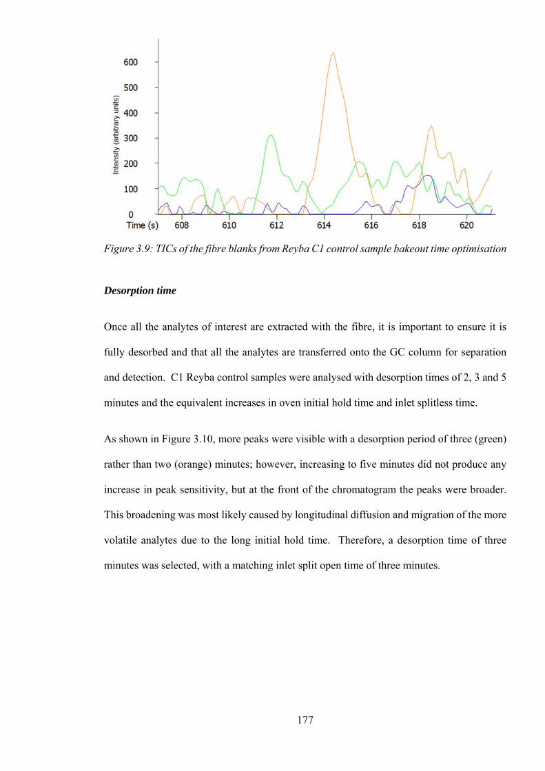
177

Figure 3.9: TICs of the fibre blanks from Reyba C1 control sample bakeout time optimisation

Desorption time

Once all the analytes of interest are extracted with the fibre, it is important to ensure it is

fully desorbed and that all the analytes are transferred onto the GC column for separation

and detection. C1 Reyba control samples were analysed with desorption times of 2, 3 and 5

minutes and the equivalent increases in oven initial hold time and inlet splitless time.

As shown in Figure 3.10, more peaks were visible with a desorption period of three (green)

rather than two (orange) minutes; however, increasing to five minutes did not produce any

increase in peak sensitivity, but at the front of the chromatogram the peaks were broader.

This broadening was most likely caused by longitudinal diffusion and migration of the more

volatile analytes due to the long initial hold time. Therefore, a desorption time of three

minutes was selected, with a matching inlet split open time of three minutes.

178

Figure 3.10: TICs of the C1 Reyba control samples from the desorption time optimisation

GC oven initial temperature hold time

Usually, the oven initial hold time will be the same length of time as the splitless time.

During the splitless period analytes are being transferred onto the GC column and if this is

increasing in temperature the transferred analyte molecules, especially those that take longer

to vapourise and transfer such as semi-volatile analytes, will not condense in the same place.

This results in band broadening of those analyse at the front end of the column before they’ve

started to be separate.

Due to the band broadening seen in the earlier experiment, the chromatograms produced

from an initial oven temperature time of two or three minutes were compared and for three

minutes the mid-later eluting peaks were no narrower than for two minutes, but the early

eluting peaks were slightly broader. Therefore, an oven initial hold time of two minutes was

chosen.

179

Summary of optimisation with the C1 Reyba control sample

A summary of the parameters optimised using the C1 Reyba control sample and used in

subsequent analyses is given in Table 3-13.

Table 3-13: Summary of optimised parameter values for the C1 Reyba control sample

Parameter Optimised value (minutes) Extraction time 12 Desorption time 3

Bakeout time 15 GC inlet split open time 3 Oven initial hold time 2

3.3.3.4 Selection of SPME fibre type

Previous method development and experience, prior to my PhD, had determined that the

CAR/PDMS was the SPME fibre that extracted the largest range of volatilities and polarities

from aqueous samples that could be seen using this analytical column. However, as will be

discussed in Section 3.3.4.1, a change in the analytical column manufacturer enabled the

maximum oven and the inlet temperatures to be raised, enabling the separation and detection

of less volatile analytes. Therefore, it was decided to compare the range of analytes that

could be extracted with three different fibres, using the conditions that had been optimised

up until this point, but with the new Restek Rxi-624Sil column. The new column enabled

the final oven temperature to be increased to 300 °C (rather than 240 °C); where it was held

for 0 minutes (rather than 2.5 minutes); making a total run time of 15.5 minutes (rather than

15 minutes).

Before experimenting with different fibre types, the chemistries of the fibre coatings and the

potential analytes were considered to determine the best three phases to try, as there are ten

different SPME fibres commercially available. A phase was required that could extract a

180

wide volatility range, a wide polarity range and extract analytes at trace levels. All the

commercially available SPME fibres were considered:

• 75/85 µm Carboxen/Polydimethylsiloxane (CAR/PDMS) is an adsorption type fibre,

which is better for trace-level analysis and good for the adsorption of volatiles with

a MW 30-225 u. This was selected as the first choice of fibre and is what had been

used in previous studies.

• 30 or 7 µm Polydimethylsiloxane (PDMS) are good for non-polar semi-volatile

analytes (Sigma-Aldrich, 2009), but a thicker coating can be used to trap any volatile

analytes, therefore a 100 µm PDMS coating was selected to extract volatile analytes

with a molecular weight (MW) between 60-275 u

• 60 µm Carbowax (CW) and 85 µm Polyacrylate (PA) are good for extracting polar

analytes such as alcohols with a MW of 40-275 u and 80-300 u. However, since the

extraction of a wide range of polarities was required, these fibres were considered

but were not tried.

• 65 µm Polydimethylsiloxane/Divinylbenzene (PDMS/DVB) is good for the analysis

of polar volatiles, amines and nitro-aromatic compounds with a MW 50-300 u.

• 50/30 µm Divinylbenzene/Carboxen on Polydimethylsiloxane (DVB/CAR/PDMS)

is good for the analysis of flavour compounds with a MW of 40-275 u.

The three fibres selected for comparison were:

• 75/85 µm CAR/PDMS

• 100 µm PDMS

• 65 µm PDMS/DVB

181

For each fibre, the first step was their conditioning in the fibre conditioning station. The

PDMS/DVB and PDMS fibres were conditioned at 250 °C for 30 minutes and the

CAR/PDMS at 300 °C for 1 hour (SUPELCO, 1999).

The inlet temperature previously had been limited to 230°C, by the maximum isothermal

temperature of the analytical column. As the fibre optimisation was carried out after the

analytical column was changed from the SGE column to the Restek column, the GC inlet

temperature could be increased to the optimal desorption temperatures for the different

fibres. They each had different maximum and recommended desorption temperatures of 270

°C (PDMS/DVB), 280 °C (PDMS) and 310 °C (CAR/PDMS), respectively. The maximum

isothermal temperature for the new column was 300 °C and to minimise bleed, a final oven

temperature of 300°C had been chosen. The inlet temperature should be below the final

oven temperature, to ensure that any higher MW analytes desorbed onto the column can

easily be eluted. Therefore, an inlet temperature of 280 °C was used for the CAR/PDMS

fibre and the PDMS fibre and a slightly lower temperature of 270 °C for the PDMS/DVB.

A summary of the fibres can be seen in Table 3-14.

After conditioning, each fibre was analysed twice, except for the PDMS/PVB that was

desorbed thrice, as it had higher bleed. No sample was extracted. The last fibre blank for

each SPME fibre was overlaid and is shown in Figure 3.11.

Table 3-14: Summary of the SPME fibre types and parameters

Parameter optimised

SPME fibre type

Conditioning temperature

(°C)

Conditioning time (min)

GC inlet temperature

(°C) Fibre type: PDMS/DVB

PDMS/DVB 250 30 270

Fibre type: PDMS

PDMS 250 30 280

Fibre type: CAR/PDMS

CAR/PDMS 300 60 280

182

Figure 3.11: Overlaid TICs of the fibre blanks for the three SPME fibres

The chromatograms were used to compare each fibre for artefacts and background noise

levels, which add extra peaks to the chromatogram and reduce the method sensitivity,

therefore a fibre with a low bleed and background was preferred. As shown in Figure 3.11,

the PDMS/DVB fibre showed by far the highest background signal throughout the

chromatogram, even after three desorptions, compared to two desorptions for the other two

fibres. The CAR/PDMS had fewer artefact peaks and they were present at much lower levels

than the PDMS/DVB. The PDMS fibre had artefact peaks present at lower concentrations

than the CAR/PDMS, but there were a few more of them. From this experiment, the

PDMS/DVB was the worst performing fibre.

Next, each fibre was used to analyse a blank, this was a prepared vial with matrix modifiers,

but the urine sample was replaced by an equivalent volume of DI water and no IS solution

was added. The chromatograms were compared between fibres and with the fibre’s fibre

blanks to check for further artefacts that could be caused by the matrix modifiers and water

183

vapour. The chromatograms from the analysis of these matrix blanks (with no IS solution),

for each of the three different fibres are overlaid in Figure 3.12.

Figure 3.12: Overlaid chromatograms of blanks (with no IS added) for the SPME fibres

The source of the additional peaks was tricky to determine, as additional peaks could have

been additional fibre artefacts or the fibre being very sensitive and picking up traces from

the matrix blank. The known artefacts from the fibre blanks were compared to see if they

were larger in the matrix blank. Although the peaks seen in the fibre blanks, for example

the two peaks between 425-450 seconds, were present in the matrix blank, they appeared to

be comparable in size. Some peaks, for example the peak at 900 seconds in the PDMS/DVB

fibre blank was much smaller in the matrix blank, this could be because repeated desorptions

had reduced the bleed.

Comparing the chromatograms in Figure 3.12, the PDMS/DVB extracted analytes around

the middle of the chromatogram, mostly from 550-860 seconds. This fibre also gave the

largest peaks between 700-800 seconds. The PDMS fibre mainly extracted analytes that

184

eluted later in the chromatogram from 740-1020 s, overall this fibre produced the smallest

peaks of the three. The CAR/PDMS extracted the most volatile analytes, producing large

peaks, with most peaks eluting between 200-800 seconds. This fibre seemed to extract the

largest range of volatilities, although it didn’t give large peaks for analytes eluting after 800

seconds compared to the PDMS fibre. If it was impurities in the matrix blank that were

being extracted, then the CAR/PDMS or PDMS/DVB fibre were better.

Finally, each fibre was used to analyse two aliquots of a clinical control sample, labelled

Goutr. These duplicates for each fibre were compared against each other for reproducibility

(there were a limited number of replicate samples from each patient and therefore further

replicates could not be analysed). The overlaid replicates for PDMS/DVB is shown in Figure

3.13; PDMS in Figure 3.14 and CAR/PDMS in Figure 3.15.

The overall reproducibility was good for all fibres, with all analytes extracted in both

replicates. There were some slight variations in response for some peaks for each fibre, but

these didn’t show a significant trend.

As seen before with the matrix blanks, CAR/PDMS appeared to extract the more volatile

analytes more effectively, with higher responses than the other two fibres. The PDMS/DVB

did not extract many volatile peaks, with the majority eluting between 500-800 s. The profile

of peaks between 500-800 s was very similar for all three fibres, this could be because all

contained PDMS. However, this is more difficult to see for the CAR/PDMS replicate

overlays, because the scale is very different.

185

Figure 3.13: TICs from the PDMS/DVB fibre analysis of a C1 Goutr control

Figure 3.14: TICs from the PDMS fibre analysis of a C1 Goutr control

186

Figure 3.15: TICs from the CAR/PDMS fibre analysis of a C1 Goutr control

The maximum response for an analyte extracted with the PDMS/DVB fibre was just over

8x10-7; PDMS just over 1x10-7; and for CAR/PDMS 1.4x10-8(all measured in arbitrary

units). This variation in response is more easily seen in the overlays of the first replicate for

each fibre, as shown in Figure 3.16.

Figure 3.16: TICs of the e analysis of C1 Goutr control samples using different SPME fibres

187

Summary

To summarise, the PDMS was good for analysing non-polar analytes but gave very poor

sensitivity for other, more polar analytes, especially the more volatile components of the

sample. PDMS/DVB gave good sensitivity for analytes with a wide range of polarities,

however it gave a high amount of fibre bleed and could only analyse a limited volatility

range. The CAR/PDMS fibre, used in the previous study, extracted analytes with a wide

range of volatilities and polarities but also had a high maximum temperature of 310 °C

making it more stable and less prone to bleed, resulting in a lower background and making

it more suitable for longer use. Therefore, it was decided to continue with the Car/PDMS

fibre as determined in previous studies.

3.3.4 Development of the HS-SPME-GC-TOFMS method

3.3.4.1 GC analytical column and oven temperature program

Initial studies had suggested that the SGE BP 624 (30 m x 0.25 mm x 1.4 µm film) gave

good separation of the analytes indicating that the stationary phase type selected was correct

for the proposed method. However, the column maximum temperature of 240 °C was being

reached and held to elute all analytes extracted with the SPME fibre. This resulted in a high

amount of column bleed at the end of the analysis and the temperature hold meant that any

less volatile analyte peaks broadened, reducing their sensitivity. After the method

development phase and first study of 4 batches of samples, but before the large study of 22

batches of samples, the column had deteriorated significantly and was causing excessive

bleed. An alternative manufacturer of the same column phase and dimensions was

identified. A column was purchased from Thames Restek (Saunderton, Buckinghamshire,

UK) and evaluated. With a maximum temperature of 320 °C, this enabled the column

temperature to be ramped to elute all the analytes desorbed by the fibre before the final

188

temperature was reached. This minimises the band broadening of peaks towards the end of

the run and ensures maximum sensitivity, if there isn’t excessive column bleed.

The bleed profile of the two columns, when new and after conditioning were compared and

it was found that the Restek column had lower bleed even though it was being heated to a

higher final oven temperature. After being used for the analysis of 22 batches of samples

for the bladder and prostate cancer projects, the Restek column was still found to have low

bleed. It was then used for the hepatic disorders project and is still in use today for relevant

projects.

With optimisation, a final column temperature of 300 °C was selected with no final hold,

which ensured that all extracted and desorbed analytes were separated and detected. No

sample analyte peaks were seen above this temperature and this allowed the column to be

kept at a temperature that minimised column bleed. The analysis of fibre blanks on the SGE

(orange) and Restek (green) columns is shown in Figure 3.17. Even though the Restek

column final oven temperature was higher temperature, there was still significantly lower

bleed than the previous column used. The final run time was 15.5 minutes.

Figure 3.17: Comparison of column bleed between the SGE and Restek columns

189

3.3.4.2 GC inlet temperature

The GC inlet and MS transfer line temperatures are limited by the maximum temperature of

the stationary phase, as the column passes into them and the temperature is held constant.

The maximum isothermal temperature of the SGE column was 230 °C which meant that the

GC inlet temperature could not be raised to the optimal desorption temperature for the SPME

fibre chosen. Ideally, the SPME fibre should be desorbed as quickly as possible and all

analytes that had been extracted from the sample with the fibre should be desorbed into the

GC, with a volatility range that can then be eluted by the column. The maximum temperature

the CAR/PDMS SPME fibre could be desorbed at was 310 °C. By changing to the Restek

column, the maximum isothermal temperature was now 300 °C.

The GC inlet temperature was optimised to fully desorb all the analytes extracted while

keeping all temperatures at a minimum, to minimise both fibre and column bleed. A value

of 280 °C was chosen, as at higher temperatures there were no noticeable improvements to

the number or size of the peaks detected.

After changes to the inlet temperature were made, there was a final check of the optimal

fibre desorption time. This was kept at three minutes, with a splitless time of three minutes.

3.3.4.2 Transfer line temperature

With an increase in the final oven temperature from 240 °C to 300 °C it is important that the

less volatile analytes eluting through the analytical column do not condense or slow their

progress when passing through the transfer line into the MS, as band broadening will occur.

As discussed in the previous section, the Restek column has a higher maximum isothermal

temperature. Subsequently, the transfer line temperature was increased from 220 °C to 280

°C to ensure all analytes eluted into the ToFMS with minimal band-broadening.

190

3.4 HS-GC-MS and TD-GC-MS of Bacterial Samples

3.4.1 Selection of the sampling technique and instrumentation

The method of sampling from BACTECTM bottles was developed at The Open University

using clean BD BACTECTM Lytic/10 Anaerobic/F and BD BACTECTM Plus + Aerobic/F

bottles (Becton, Dickinson and Company (BD), New Jersey, USA), containing only the

medium and no blood sample. Due to the difficulty in obtaining samples, especially any

replicates for the pilot study, the parameters were not optimised but were selected based on

calculations and available information.

Due to the nature of the samples, a sampling technique for the pilot project was required that

could sample directly from the BACTECTM bottles that had been prepared and analysed

using conventional methods for identification of the bacteria type, rather than taking a sub-

sample of this for analysis. The BACTECTM bottles are too large to fit into the autosampler

without modification, therefore a more manual technique was required.

Manual headspace, SPME and TD sampling were the three techniques evaluated for volatiles

analysis. Manual SPME analysis can be more difficult, as the sample needs to be heated and

shaken for a period with the SPME fibre inserted in the sample, before being retracted and

inserted into the GC inlet. Manual HS, in some ways is more simple, as the headspace can

be removed and injected directly into the GC inlet; although, if the sample is at a higher

temperature the syringe would need to be at a higher temperature to prevent condensation of

less volatile analytes. HS analysis would require the sample to be next to the instrument,

whereas sampling with SPME fibres enables sampling in a remote location before being

thermal desorbed in the GC inlet.

191

Due to the nature of the samples and the fact that the instrument was not in a fume hood, nor

could a filter be employed to prevent sampling of bacteria directly onto the fibre, it was

decided that SPME should not to be used for the pilot study.

TD uses active sampling onto a tube, through a filter to prevent the sampling of bacteria into

the tube. Sampling can also be carried out at a remote location away from the instrument,

as the TD tubes can be sealed and heat treated to sterilise any live bacteria, which could

possibly have transferred to the tube during the sampling process. Two different candidate

sampling methods were developed, HS and TD.

The Unity TD system was connected to an Agilent 7890-5975C GC-MS for the initial pilot

project. The Unity TD was evaluated with the addition of an ULTRA autosampler and these

were then semi-permanently installed on an Agilent 6890-5973 GC-MS. The Leco GC-

ToFMS was unavailable for the pilot project as it was being used for the urine projects.

3.4.2 Development of the sampling methods

3.4.2.1 HS analysis

At the Open University (OU), the first method was developed using HS analysis. The aims

were to see if volatile analytes could successfully be removed and analysed by the technique

and to see if there were any large interference peaks from the sampling technique or the

BACTECTM bottle, such as plasticisers.

Sampling method

A 2.5 mL gas-tight HS syringe fitted with a 0.22 µm filter (Merck Millipore, Billerica,

Massachusetts, USA), was used to withdraw 2.5 mL of the headspace from the blank

BACTECTM bottle. It was directly injected and analysed using the same method for HS-

GC-MS as described in Section 2.3.2.3. The same column was used as at UCLH. The only

192

difference was that the injections were made into the injection port of an Agilent 7890-

5975C GC-MS instead of a Shimadzu QP2010 GC-MS.

Analysis of blank BACTECTM bottles

Comparisons were made between sampling the headspace in the BACTECTM bottle and the

laboratory air. As is shown in Figure 3.18, there is a clear difference with more peaks from

the BACTECTM bottle headspace (blue), but fortunately there are no large interfering peaks.

This result meant that we were successfully removing VOCs from the BACTECTM bottle

with both the bottle and the syringe at ambient temperatures.

Figure 3.18: TICs of the HS sampling of laboratory air vs. BACTEC bottle

Microbial filter contamination check

Comparisons were also made between sampling the laboratory air with and without a

microbial filter to check for contaminants such as phthalates, from the filter. The m/z 149

ion, the common fragment ion for phthalates, was extracted from the chromatogram (an EIC)

to look for these contaminants. As can be seen in Figure 3.19, none were visible.

2.00 4.00 6.00 8.00 10.00 12.00 14.00 16.000

100000

200000

300000

400000

500000

600000

700000

800000

900000

Time-->

Abundance

TIC: LabAir2.D\data.msTIC: BACTEC.D\data.ms (*)

193

Figure 3.19: EIC m/z 149 of HS sampling of laboratory air with & without a microbial filter

The key ions for hydrocarbons, m/z 43 (black) and 57 (blue), were also extracted. As can

be seen in Figure 3.20 some hydrocarbons were present, as expected, but not in large,

problematic amounts. Also, not all peaks are hydrocarbons, for example the peak at 6.6

minutes is acetone from the laboratory air.

Figure 3.20: EIC m/z 43 u for the HS analysis of laboratory air with microbial filter

2.00 4.00 6.00 8.00 10.00 12.00 14.00 16.000

500

1000

1500

2000

2500

3000

3500

4000

4500

5000

5500

6000

6500

7000

7500

8000

8500

9000

9500

10000

10500

11000

Time-->

Abundance

Ion 149.00 (148.70 to 149.70): LabAir.D\data.msIon 149.00 (148.70 to 149.70): LabAir2.D\data.ms (*)

2.00 4.00 6.00 8.00 10.00 12.00 14.00 16.000

500

1000

1500

2000

2500

3000

3500

4000

4500

5000

Time-->

Abundance

Ion 43.00 (42.70 to 43.70): LabAir2.D\data.msIon 57.00 (56.70 to 57.70): LabAir2.D\data.ms

194

3.4.2.2 TD analysis

Sorbent selection

The second method involved concentrating a sample using a TD tube packed with a sorbent.

The sorbent was selected by considering the volatility and polarity of the analytes and the

nature of the matrix. Blood contains water and on heating of the sample to 37 °C, the

incubation temperature of the bacterial samples, would cause a humid environment.

Therefore, the best sorbent type would be hydrophobic. We had no idea what the volatility

range of the analytes present would be, at 37 °C they would be volatile to semi-volatile

compounds and therefore would require more than one sorbent. Analytes could have a range

of polarities, with likely compound classes being more polar species such as acids,

aldehydes, ketones, etc. (Schulz & Dickschat, 2007). The main two options for sorbents,

were Tenax® TA/Unicarb or Tenax® TA/Carbograph 5TD.

Unicarb is a carbonised molecular sieve that has been subsequently replaced by Sulficarb, it

is good at trapping light VOCs from C3-C8 with boiling points of -30 to 150 °C and sulphur

species as it is inert. It is a stronger sorbent than Carbograph 5TD, giving better

breakthrough volumes, but it also absorbs water as it is slightly hydrophilic. Carbograph

5TD is a medium-strong sorbent, suitable for the light hydrocarbon range of analytes from

C3/4-C8 with boiling points of 50 to 150 °C, but is also good for trace-level applications as it

gives minimum artefacts on heating and is hydrophobic. However, it can have some activity

with labile compounds. Tenax® TA is a porous polymer that has a weak strength with low

inherent artefacts. It is inert and is hydrophobic and it is good for trapping and releasing

analytes from C6-C26 with boiling points from 100 to 450 °C (Markes International Ltd.,

2012). After considering the possible analytes and matrix and with advice from the

manufacturer (Markes International Ltd., Pontyclun, Wales), for the preliminary studies a

dual-sorbent TD tube was selected. This contained Tenax® TA with a mesh size of 35/60 to

195

ensure small particles of Tenax® didn’t leak through the retaining gauze at the

sampling/desorption end of the TD tube, and Carbograph 5TD with a mesh size of 40/60

sorbents were selected. The sorbents were held in stainless steel TD tubes. These were

originally purchased as pre-conditioned tubes from the manufacturer, due to the urgency of

the project at the time and the fact that no autosampler was available for automated

conditioning. After use, the tubes were re-conditioned ready for re-use by following the

manufacturer’s recommendations.

Sampling system set-up

In the OU laboratory, various ways were tried to successfully connect the pump to the TD

tube and then the sampling end of the TD tube to the syringe, via a filter, without any

leakages occurring. Medical grade tubing was used between the needle and the TD tube, as

this produces low artefacts and should be inert. The final set-up, as shown in Figure 2.2,

included the pump connected to the TD tube using low flow tubing, as only small volumes

of headspace would be collected, unlike other TD applications where litres of gas-phase

samples are frequently collected. The sampling end of the TD tube was then connected to a

disposable filter system using a short length of medical grade tubing which was connected

to the disposable needle. The needle was then inserted into the BACTECTM bottle.

Selection of sampling parameters

After incubation of the BACTECTM bottle there would be a high concentration of volatiles

in headspace above the medium, therefore it was decided to extract these under static HS

conditions but drawing out the headspace through the TD tube using the pump, to ensure no

volatiles were lost to the atmosphere. Once the pump was drawing out the headspace, a

second needle could be inserted to replace the air being withdrawn from the bottle and

therefore now the sampling would be dynamic HS, where volatile analytes emerging from

the sample would immediately be swept away to the TD tube. The volume of the

196

BACTECTM bottle is 80 mL. It is filled with 30 mL of aerobic bacteria growing medium or

40 mL of anaerobic bacteria growing medium. With a maximum sample of 10 mL, this

leaves 30-40 mL of headspace, depending on the type of bottle.

This is a small volume for TD sampling and sampling is through a narrow i.d. needle.

Usually, the optimal sampling rate through a standard 5 mm i.d. packed TD tube is 50

mL/min, with a working range of 10-200 mL/min for sample volumes of 500 mL and higher.

The minimum flow for trapping is 10 mL/min, therefore a flow rate of 20 mL/min was

selected, to allow for any variation in pump flow, sampling set-up, etc. The amount of time

sampling under static flow conditions needs to exceed the time taken to remove the volume

of headspace, again to account for any variability. 40 mL of headspace sampled at 20

mL/min would take 2 minutes to evacuate, therefore a time of 10 minutes was selected, for

both the static HS and then the dynamic HS sampling. These values were not optimised for

the pilot study, but were on the list for optimisation for the full study. This method was then

applied to check that volatiles were extracted from the blank BACTECTM bottles.

Analysis of blank BACTECTM bottles

As shown in Figure 3.21, comparisons were made between sampling the headspace in the

BACTECTM bottle (black) and the laboratory air (blue). A clear difference can be seen with

more peaks present than in the headspace method and some different peaks which were

identified as TD tube artefacts, by comparison with a conditioned TD tube that had not been

exposed to samples.

The TD method was, as expected, more sensitive than the HS method for concentrating

peaks from the BACTECTM bottle.

197

Figure 3.21: TICs of the TD sampling of laboratory air vs. BACTEC bottle

Tubing and microbial filter contamination check

Comparisons were also made between sampling the laboratory air with and without the

tubing and microbial filter, to check for contaminants such as phthalates, etc. from the tubing

and filter. No ions of m/z 149 u were seen, the EICs for m/z 43 and 57 u are shown in Figure

3.22 . Some small hydrocarbon peaks were seen, but again these peaks from the tubing and

filter were minimal.

2.00 4.00 6.00 8.00 10.00 12.00 14.00 16.00 18.00 20.00 22.000

50000

100000

150000

200000

250000

300000

350000

400000

450000

500000

550000

600000

650000

700000

Time-->

Abundance

TIC: TD_BACTEC.D\data.msTIC: TD_LabAir.D\data.ms (*)

198

Figure 3.22: EICs m/z 43 and 57 u for the TD analysis of laboratory air with the microbial

filter

3.4.3 Development of the HS-GC-MS analysis method

The HS-GC-MS method needed to have a fast analysis time, as we only had access to the

Biochemistry Department GC-MS instrument for 1 day, which had to include the HS and

TD sampling methods too.

3.4.3.1 HS-GC-MS column selection

The standard 624 column phase for VOCs analysis was chosen again. A spare SGE BP624

column (30 m x 0.25 mm i.d. x 1.4 µm) from the urine sample work was sent down in

advance for installation into the Shimadzu GC-MS at UCLH.

3.4.3.2 HS-GC-MS method development

A fast method was developed at the OU for the analyses at the same time as the sampling

method was developed.

2.00 4.00 6.00 8.00 10.00 12.00 14.00 16.00 18.00 20.00 22.000

2000

4000

6000

8000

10000

12000

14000

Time-->

Abundance

Ion 43.00 (42.70 to 43.70): TD_LabAir2.D\data.msIon 57.00 (56.70 to 57.70): TD_LabAir2.D\data.ms

199

GC inlet mode and parameters

HS analyses uses a split injection to transfer the volatile analytes very quickly onto the

analytical column for separation. The higher the split ratio, the faster the transfer but also

more of the sample goes to waste and therefore sensitivity drops. A split ratio of 10:1 was

selected as a compromise but this could not be tested at The OU as there were no ‘real’

samples. During the sample analysis at UCLH, the sensitivity of the first sample analysed

was low and so the split ratio was reduced to 5:1 to help improve the sensitivity of the

method, through an increase in the sample transferred on to the column.

GC oven temperature program

With split injections, the transfer to the column is very fast and therefore the focusing of the

more volatile analytes on the front end of the column is less necessary. An initial oven

temperature of 50 °C with a hold time of 0.5 minutes was long enough to give more than

two flushes of the liner volume and to separate the more volatile analytes on the column,

while minimising the run time and the oven cool-down time. A ramp rate of 15 °C was a

compromise between getting a good separation of the analytes while minimising the run

time, this value was selected based on previous experience. The maximum ramping

temperature of the SGE BP624 column is 240 °C and therefore during the run, the oven

temperature was ramped to 240 °C and held for 1 minute.

A column flow of 1 mL/min in helium was selected to give an average velocity of around

36 cm/s, the optimal velocity range for helium is 20-40 cm/s and therefore 36 cm/s would

still give a good resolution while minimising run time. On inputting this method into the

Shimadzu instrument, the software preferred 0.98 mL/min calculating the pressure to be at

54.7 kPa.

200

MS transfer line (interface) temperature

The GC-MS interface temperature was selected as 220 °C to give minimal bleed into the

MS, while not allowing condensation of the analytes while moving through the transfer line.

MS method

The low mass of m/z 33 u was selected to be as low as possible to see more ions in the mass

spectra of the more volatile analytes, while avoiding acquiring the oxygen molecular ion at

m/z 32 u and nitrogen molecular ion at m/z 28 u. Both of which are abundant when analysing

samples that can contain air (as these were used BACTECTM bottles). Their exclusion avoids

saturating the MS and causing noisier baselines. Also, a solvent delay of 0 was selected, due

to the lack of a solvent peak, the scan range starting higher than the sample matrix (air) and

to ensure no very volatile analytes were missed with the higher initial oven temperature. A

high mass of 300 u was selected, as this was believed to be the maximum MW of analytes

sampled by HS analysis. Dr John Honour, the operator of the Shimadzu GC-MS,

recommended an ion source temperature of 220 °C, a threshold value of 10 and event time

of 0.25 s for the mass range acquired and for the chromatographic peak widths of the analytes

as seen during the method development at the OU laboratory.

HS injection volume

A maximum of 2.5 mL of headspace was injected, as this was the maximum volume of the

HS syringe and a larger headspace injection volume would also increase the volume of water

vapour injected into the GC, that could cause interferences with the separation of the

analytes.

201

3.4.4 Development of the TD-GC-MS analysis method

The analysis of volatile analytes by TD-GC-MS is a common application. The GC-MS

separation suffers little from matrix effects, if the TD tube sorbent is carefully selected for

the application and the amount of sample transferred to the GC column is optimal.

Therefore, matrix effects affecting retention time reproducibility should be relatively low.

Alignment of the GC-MS traces is one of the first steps in chemometric analyses and is

important for detecting differences between the samples. Therefore, reproducible retention

times can minimise the effort required and make the alignment easier.

3.4.4.1 Retention Time Locked (RTL) method and database

RTL

The TD-GC-MS analyses were performed on a Markes International TD system, hyphenated

to an Agilent GC-MS system. The accuracy of the EPC pressure control, in psi, is 2 decimal

places on the older 6890N GCs and 3 decimal places on the newer Agilent 7890 GC.

One of the key features of the Agilent acquisition software is the ability to retention time

lock (RTL) the method to one analyte (RTL compound), preferably eluting around the

middle of the chromatogram. The method is then always locked to that analyte eluting at

that retention time enabling all the other analytes to have the same retention times from run-

to-run, batch-to-batch, instrument-to-instrument and after maintenance by relocking the

method. The method is retention time locked by acquiring five runs in constant pressure

mode, which is more accurate than constant flow mode as flow is a calculated value whereas

pressure is absolute. In each run the pressure is changed and an analysis is performed of a

conditioned TD tube, spiked with the RTL compound using the spiking rig. This results in

the generation of a 5-point calibration of the retention time of the RTL compound versus

202

pressure. From that, the software can then calculate the pressure required to enable the

locking compound to elute at the locked retention time.

RTL library

Agilent has developed multiple libraries for different industries using a locked method and

therefore the retention times of the compounds along with the mass spectrum can be used

for the identification of target analytes in screening and quantitative analyses. This is

particularly useful when analysing suites of compounds containing isomers, that have the

same mass spectra and therefore the exact isomer must be identified by its retention time.

A locked method and library for use with TD-GC-MS is the indoor air toxics retention time

locked library (IARTL) (Wylie, et al., 5989-5435EN) containing 171 compounds. This RTL

database was available for use on the TD-GC-MS instrument used for the bacteria samples.

The library was designed for the analysis of indoor air toxic volatiles, however many of the

analytes present are common VOCs and I have used it for many applications during my

work.

RTL compound

The method is retention time locked to toluene-d8 or toluene. I chose toluene as this was

available in the laboratory. The method was locked to toluene at 12.468 minutes. This

means that the remaining 170 compounds in the IARTL library will then elute at the retention

times suggested in the library, if the same analytical column and analysis parameters are

used.

3.4.4.2 TD-GC-MS method

As the IARTL method was being followed, the GC separation and MS detection parameters

were taken from this and therefore did not require optimisation. These parameters are

203

specified in Section 2.3.3.4. This includes the DB-VRX column that is a manufacturer

specific modified version of a 624 column for VOC analysis.

Many parameters were taken from the TD method, however the IARTL method uses a TD

tube packed with Tenax® TA only, whereas the best sorbents for this application were

determined to be Tenax® TA/Carbograph 5TD.

Optimisation of the TD method

The Tenax® TA/Carbograph 5TD sorbent combination has a maximum desorption

temperature of 350 °C and a maximum recommended temperature of 320 °C (Markes

International Ltd., 2014). Lower desorption temperatures reduce artefacts and extend

sorbent lifetime.

For the method, a TD tube desorption temperature of 300 °C was set and held for 10 minutes

to ensure the tube was fully desorbed onto the cold trap, while minimising the temperature.

The cold trap desorption split ratio was a comprise between ensuring a rapid transfer to the

analytical column to obtain narrow sample bands and therefore sharp peaks and a large

proportion of the sample going to waste and reducing sensitivity. An optimal 15:1 to 20:1

split ratio should ensure good sensitivity and fast transfer through the long transfer line from

the TD instrument to the column, however on the Unity the flows are set using a flow meter

and needle valves and therefore it is easier to set the cold trap desorption split flow at a

rounded up or down number to ensure reproducible set-up batch-to-batch. The split flow

was set at 40 mL/min, resulting in an 18.6:1 split ratio.

Summary of the TD-GC-MS RTL method

The reasons for using this RTL method rather than developing a separate method based on

the urine methods are that the RTL reduces data alignment in chemometric analysis. This is

especially useful if batches of samples were to be analysed periodically, with the analytical

204

instrument used for other applications with different set-ups in-between. Also, if after

chemometric analysis peaks were highlighted that could be potential biomarkers, these could

quickly be identified if they were either already within the library, or they could be easily

added to the library for subsequent routine screening and quantitation. As this was a pilot

study, using the RTL method saved lots of time rather than developing the GC-MS method.

The RTL method had already been developed, optimised and proven for VOCs in TD-GC-

MS analysis using a single quadrupole MS. The method I had developed for urine analysis

by HS-SPME-GC-MS was using a ToFMS that has a higher acquisition rate then SQMS and

therefore can detect narrower peaks and produce more data throughout a shorter run time.

Therefore, the use of the urine method for this study was not applicable for the instruments

used.

205

Bladder Cancer Study

206

4.1 Introduction

Dogs have been trained to recognise specific volatiles from the headspace above urine

samples to detect bladder cancer (Willis, et al., 2004), but their use for routine clinical

analysis is limited. GC-MS is an analytical technique that is already used in hospital

laboratories that is also good at separating and detecting volatile organic compounds

(VOCs). SPME is a technique that is good at extracting and concentrating VOCs for

desorption into a GC-MS (Pawliszyn, 2011).

Following on from the promising results of the preliminary trial described in Chapter 3, a

much larger study of the samples was analysed by HS-SPME-GC-ToFMS using the

optimised method described in Chapter 2.

4.1.1 Participant selection

Participants were recruited for both the bladder cancer and prostate cancer studies at the

same time. Patients presented with new or recurrent transitional cell carcinoma (TCC) of

the bladder or prostate cancer at Buckinghamshire Healthcare NHS Trust. The study was

given favourable ethical opinion by the Mid and South Buckinghamshire Local Research

Ethics Committee (04/Q1607/65) and all participants gave written informed consent.

Participants completed a Case Report Form (CRF) providing considerable detail about their

medical, personal and social histories to enable any medical or lifestyle factors to be taken

into consideration that might influence the chemical composition of their urine.

The co-ordination of taking, processing and storing the samples and patient details was

undertaken by Dr Carolyn Willis and Mrs Lezlie Britton at Amersham Hospital. Samples

were taken in the Urology Department before any surgical or therapeutic intervention. Urine

cytology and biochemistry tests were conducted at Wycombe Hospital. This process was

207

described in Section 2.2.2. The data was then anonymised before information and samples

were sent to The Open University for analysis.

4.1.2 Bladder cancer and control sample types

The samples for the bladder cancer study were divided into two classes, those with

transitional cell carcinoma bladder cancer (TCC) and controls (C) with no bladder cancer.

Each of the classes were sub-divided into categories.

For the study, samples from all TCC participants were used. Participants from each of the

three control categories were randomly selected to match the total number of TCC

participants, as advised by Cranfield University to reduce any bias in the data analysis.

For all the samples analysed, I extracted the metadata by highlighting the range of values

from each data type or highlighting those that tested positive for a feature. A screenshot of

the sex, age, smoking status and dipstick measurements for some of the TCC2 and TCC3

participants can be seen in Figure 4.1. A screenshot of the diagnosis and the medication

taken up to 48 hours before the study sampling, for some of the C2 participants, can be seen

in Figure 4.2. A screenshot of the food and drink intake up to 48 hours before the study

sampling for some of the C3 participants can be seen in Figure 4.3.

Some of the participants had drunk alcohol within 24 hours, most had eaten cooked garlic,

raw garlic, cooked onion, raw onion, brassicas, mustard, mint, fish, strong cheese or other

strong food, for example ginger and spices. A handful of participants across all classes had

eaten asparagus, aniseed or liquorice in the previous 48 hours.

208

Figure 4.1: A snapshot of the metadata for TCC2 and TCC3 participants, showing sex, age, smoker and urinalysis results

209

Figure 4.2: A snapshot of the metadata for Control 2 participants, showing diagnosis and medication taken within 48 hours prior to study

210

Figure 4.3: A snapshot of the metadata for Control 3 participants, showing food and drink intake during 48 hours prior to study

211

TCC samples were taken from patients with new or recurrent bladder cancer and included

male and female patients aged over 18 years. TCC samples can be divided into three

categories by the stage of the cancer with TCC1 being early stage and TCC3 being late stage:

• TCC1 – low grade or well differentiated transitional cell carcinoma. These were

male and female patients aged between 58-87; the majority were non-smokers.

TCC1 patients had no positives on the urine dipstick test for glucose, bilirubin or

nitrite; some had trace amounts of ketones and some tested positive for leucocytes;

most tested positive for protein and/or blood; they had normal urobilinogen levels

except for one patient; their urine ranged from pH 5-7; the majority were taking

prescription medication; half were taking over the counter medication pain relief or

indigestion; some were on vitamin or mineral supplements; no one had taken

recreational drugs.

• TCC2 – moderately differentiated transitional cell carcinoma. These were male and

female patients aged between 49-86; a mixture of smokers and non-smokers. TCC2

patients had no positives on the urine dipstick test for nitrite; some had trace amounts

of ketones and some tested positive for glucose and/or leucocytes; most tested

positive for protein and/or blood; one tested positive for bilirubin and two for high

urobilinogen levels; their urine ranged from pH 5-7.5; the majority were taking

prescription medication; most were not taking over the counter medication, a few

had pain relief or indigestion medication; some were on vitamin or mineral

supplements; no one had taken recreational drugs.

• TCC 3 – high grade or poorly differentiated transitional cell carcinoma. These were

male and female patients aged between 49-91; a mixture of smokers and non-

smokers. Some TCC3 patients had trace amounts of glucose and ketones in their

urine; some tested positive for bilirubin and nitrite; the majority tested positive for

leucocytes, protein and blood; two had high urobilinogen levels; their urine ranged

212

from pH 5-7.5; the majority were taking prescription medication; most were not

taking over the counter medication but a few had pain relief medication; some were

on vitamin or mineral supplements; no one had taken recreational drugs.

For the control samples, it was important to include patients with inflammation, infection

and necrosis that did not have bladder cancer, so that samples were classified purely based

on the cancer volatiles rather than volatiles that were symptoms but not specifically

attributed to the cancer. The control samples for bladder cancer included male and female

participants aged over 17 years who had a non-malignant urological disease or were healthy.

The control (C) class was divided into three categories:

• C1 – male and female healthy individuals aged between 18-34; a mixture of smokers

and non-smokers. C1 controls had no positives on the urine dipstick test for glucose,

bilirubin, ketones, protein, nitrite; leucocytes were negative but there were a few with

a trace and one with a moderate amount; they had normal urobilinogen levels; their

urine ranged from pH 5-8; most were not taking prescription medication, but some

were on asthma medication or contraceptives; most were not taking over the counter

medication but some were on pain relief; some were on vitamin or mineral

supplements; a few had taken recreational drugs.

• C2 - male and female individuals aged between 17-31; a mixture of smokers and

non-smokers. C2 controls had normal levels of urobilinogen; were negative for

bilirubin; but their urine had produced a dipstick reading that was positive for

glucose, ketones, leucocytes, nitrite and/or blood; or who had trace amounts of

protein; their urine ranged from pH 5-8; many were not taking prescription

medication the rest were on contraceptives or antibiotics; most were not taking over

the counter medication but some were on pain relief; some on vitamin or mineral

supplements; a few had taken recreational drugs. This category included any non-

cancerous condition or disease, including menstruating women, pregnancy, eczema,

213

irritable bowel syndrome, psoriasis, penile warts, thrush and those with suspected

urinary tract infections.

• C3 - male and female patients aged between 24-88; a mixture of smokers and non-

smokers. Except for 2 patients, all C3 controls had normal levels of urobilinogen.

Their urine had produced a dipstick reading that was positive for glucose, bilirubin,

ketones, leucocytes, nitrite, protein and/or blood; their urine ranged from pH 5-8.5;

most were taking prescription medication; most were not taking over the counter

medication but some were on pain relief; some on vitamin or mineral supplements;

a few had taken recreational drugs. This category included patients with a confirmed

non-cancerous urological disease including renal and ureteric stones, renal cysts,

renal colic, urethral stricture, nephrectomy, polypoid, interstitial or catheter cystitis

or stress incontinence and some were diabetic.

Control participants over the age of 32 were required to have been screened with a recent

cystoscopy to check that there were no visible signs of bladder cancer, otherwise they were

excluded.

For both control and TCC participants, men over the age over 50 were only included in the

study if they had recently been checked for prostate cancer and received a negative result.

Participants with current history of malignancy or pre-malignancy elsewhere in the body, a

pre-malignant urological disease or a history of bladder cancer other than TCC were

excluded from the study. Participants who had suffered from a different cancer elsewhere

in the body more than five years previously and were considered disease-free were included

in the study. Participants with mental incapacity or who had participated in another clinical

trial during the study period and three weeks prior to inclusion were also excluded.

214

4.1.3 Participant urinalysis results

Control 1 samples showed no urine abnormalities on dipstick. However, C2, C3 and TCC

categories did show urine abnormalities. These urinalysis abnormalities can indicate a range

of problems. The presence of:

• Blood could be caused by several disorders, including menstruation, trauma,

infection, inflammation, infarction (blood supply obstruction), neoplasia (abnormal

tissue growth). Transient blood could also be due to recent strenuous physical

activity.

• Leucocytes and/or nitrites could indicate an infection, whereas blood, leucocytes,

protein and nitrites could indicate a urinary tract infection.

• Protein could be from a range of causes, including high urine concentration, the use

of antibiotics, renal problems or recent sexual activity.

• Glucose is usually caused by diabetes or certain drugs.

• Ketones could be caused by diabetes, pregnancy, a high fat diet or starvation.

• Bilirubin and/or high urobilinogen indicates various liver problems.

The normal urine pH range is 5.5 – 6.5, but can vary from 4.5 – 8.5. High pH (alkaline) can

be caused by diet, certain drugs and several conditions, including:

• A vegetarian diet which is rich in citrus fruits, most vegetables and legumes.

• Urinary tract infections.

• Pyloric (or gastric outlet) obstructions.

• The use of certain prescription drugs that make the urine more alkaline to help

prevent kidney stones.

• Kidney failure.

• Certain metabolic disorders.

215

Low pH (acidic) can be caused by diet and several conditions, including:

• A high protein diet or certain fruits like meat and cranberries.

• Certain metabolic disorders.

• Diabetes.

• Kidney stones.

• Dehydration, starvation, diarrhoea or malabsorption.

• Certain rare conditions.

In the Control 1 group the urine pH ranged from 5 to 8. All those participants with acidic

urine of pH 5, were taking salbutamol or a similar prescription medicine. Those participants

with an alkaline urine of more than pH 6.5 had no other metadata that could explain the high

pH, therefore this could be assumed to be due to diet.

The other two control categories C2 and C3 both showed a similar trend, with pH ranging

from 5 to 8 or 8.5, respectively. Those with acidic pH had urinary tract infections, kidney

problems or were taking prescription medicines. Those with alkaline pH could not be

explained by the metadata and so this was also assumed to be due to diet.

The three TCC categories, showed a narrow range of pH, from 5 to 7.5. Acidic pH can be

explained as before. The pH neutral urine samples showed no match to the metadata and

therefore again was assumed to be diet related.

The specific gravity measures the ability of the kidney to concentrate or dilute the urine. It

measures the amount of solute dissolved in urine and is compared to the density of water

(1.000). A normal range is 1.002 to 1.035 for adults, if kidney function is normal (Fischbach,

2004).

A low specific gravity can be caused by:

• An inability to concentrate urine or excessive hydration.

216

• A range of conditions, including diabetes, renal diseases, kidney infections.

• Alkaline urine.

A high specific gravity can be caused by:

• An inability to dilute urine or dehydration.

• A range of conditions, including diabetes.

• Protein in the urine.

Across all the categories there was only one sample outside of the normal range. This was

a Control 1 participant with a specific gravity of 1. This could be assumed to be a typo in

the data or be caused by excessive hydration. However, the sample was alkaline, at pH 7.5,

with a moderate amount of leucocytes and blood. This patient was excluded in the outlier

removal.

4.1.4 HS-SPME-GC-ToFMS study samples and analysis

4.1.4.1 Samples used in the study

A total of 86 bladder cancer samples and 219 control samples were analysed in triplicate,

where the quantity of sample allowed. Analyses were conducted in 22 batches, including

fibre blanks, sample blanks and procedural blanks. The samples were prepared and analysed

using HS-GC-MS as described in Section 2.2. The total number of participants and total

number of samples analysed, including replicates for each category, along with the metadata

is presented in Table 4-1 and Table 4-2.

The data was processed using the methods described in Section 2.4. In brief, a consistency

test was initially performed on the data files to ensure that they had roughly the same number

of scans. Any files that had too few scans for alignment, were removed. Generally, these

data files were from samples that had failed to acquire on the GC-MS instrument. This

217

consistency test was performed when importing the data files into the data analysis software.

The total number of sample data files data processed beyond this step is shown in Table 4-1.

Next, the data was standardised against the IS, phenol-d6, quantitation ion. Exploratory

PCA analysis was performed and outliers were removed. Outlying samples were identified

visually and statistically, leaving the total number of participants for each category as shown

in Table 4-1.

Table 4-1: TCC and Control participants used in the study, no age-matching

Category Number: C1 C2 C3 TCC1 TCC2 TCC3 Participants 73 73 73 21 32 33 Total samples analysed 218 212 208 53 90 83

Males 26 13 26 15 21 20 Females 47 60 47 6 11 13

Smokers 23 17 25 2 11 6 With blood detected 4

(*) 41

(*-***) 52

(*-***) 9

(*-***) 14

(*-***) 31

(*-***) With glucose detected 0 2

(**-***) 3

(*-***) 0 3

(**-***) 1

(*) With protein detected 3

(*) 17 (*)

25 (*-***)

8 (*-***)

11 (*-***)

22 (*-**)

With bilirubin detected 0 0 5 (*)

0 1 (*)

5 (*-***)

With high urobilinogen 0 0 2 1 2 2 With nitrite detected 0 4

(*-***) 8

(*) 0 0 6

(*-***) With leucocytes detected 3

(*-**) 31

(*-***) 36

(*-***) 3

(*) 5

(*-**) 24

(*-***) With ketones detected 0 3

(*) 7

(*) 3

(*) 2

(*) 6

(*-**)

Total samples data processed

210 204 195 53 84 80

Participants after outlier removal

70 71 64 17 28 27

* = trace or small amount, ** = moderate amount, *** = large amount

218

The chromatographic peaks were aligned using COW. Different types of scaling and feature

selection were investigated. Classification was performed using PLS-DA, SVM-LIN and

RFs with cross-model validation through bootstrapping with LOO-CV and LFO-CV. Each

of these approaches were previously described in detail in Chapter 2.

Generally, the control samples included a higher proportion of females to males, whereas

the TCC samples had a higher proportion of males to females. Most participants in each

category were non-smokers. The percentage of smokers in each category ranged from 9 to

34 %.

Table 4-2: Participants used in the study age, pH and specific gravity, no age-matching

Category Age range (years) pH range Specific gravity range C1 18-34 5-8 1.005-1.030 C2 17-31 5-8 1.005-1.030 C3 23-88 5-8.5 1.005-1.030 TCC1 58-87 5-7 1.005-1.030 TCC2 49-86 5-7.5 1.005-1.030 TCC3 49-91 5-7.5 1.005-1.030

As shown in Table 4-2, C1 and C2 controls were all under the age of 35, as they were far

less likely to have a urological disorder. C3 controls with non-cancerous urological

disorders had a much wider age range.

It can also be seen that the pH range of the samples for each category was similar. The most

acidic pH for each category was pH 5, whereas the most basic samples ranged from pH 7 to

8.5, with controls pH 8-8.5 and TCC samples pH 7-7.5. The specific gravity for each

category had the same range of 1.005-1.030.

219

4.1.4.2 Age-matched sample set

A paper was submitted for publication about this work. Following feedback from one

reviewer, it was decided to reduce the C3 data set to only classify samples from participants

in the C3 category within the same age range as the TCC class of samples. Information on

the age-matched data set (C3(AM)) used for pattern recognition is presented in Table 4-3

and the results are discussed in Section 4.2.3. The paper, utilising the age-matched C3(AM)

data set, was subsequently accepted for publication in May 2016 (Cauchi, et al., 2016) by

Analytical Methods. This paper is in Appendix A.

Table 4-3: Participants used in the age-matched data set

Category: C1 C2 C3 TCC1 TCC2 TCC3

No. of participants after age-matching

70 71 46 17 28 27

Age range (years) 18-34 17-31 50-88 58-87 49-86 49-91

4.2 Results and Discussion

The results and discussion section is divided into four sections:

• The raw data that was processed using the Leco ChromaTOF software and was not

processed by Cranfield University will be discussed in Section 4.2.1. This data was

used to assess the reproducibility of the analytical method across all 22 batches of

samples and to evaluate the importance of using an IS. Different types of blanks

were also used to look for carryover within the analytical instrument and the sample

preparation. As both the bladder cancer study and prostate cancer study samples

were analysed together, the results for both studies will be presented here, as they

cannot be separated for certain tests. Where possible, any data that could be

separated for the prostate cancer samples, will be presented in Chapter 5.

220

• The results obtained by Cranfield University on the statistical analysis of the disease

classification models, developed using the above analytical data, will be shown and

discussed in Section 4.2.2. This section will give the results from each step of the

development of the data processing algorithms.

• The statistical analysis results from the use of the age-matched C3 samples will be

shown and discussed in Section 4.2.3.

• Finally, the results from biomarker discovery by Cranfield University will be shown

and discussed in Section 4.2.4.

4.2.1 Robustness of HS-SPME-GC-TOFMS analysis method in

the bladder and prostate cancer samples batches

As previously determined by HS-SPME-GCxGC-MS, in the method development chapter,

there are thousands of VOCs present in the headspace above urine. The GC method was

optimised to get the best resolution of all peaks seen. However, as to which peaks are the

most important ones is unknown, the calculation of the resolution of those peaks was not

possible, as would be carried out in target analysis. In this study, the analytes of clinical

interest present in the samples are unknown; therefore, standards could not be prepared to

check the linearity of the instrument for those analytes, their reproducibility nor their limits

of detection.

However, the quality control checks that could be carried out for this analysis method for

‘unknowns’ included: making sure that the instrument operated reproducibly, with similar

sensitivity between batches as well as across batches; checking that carryover was not

present or was at a very low level that didn’t interfere with the next analysis; ensuring that

any differences between samples was due to the characteristics of the sample rather than the

analysis method. In order to achieve this, an IS was used.

221

4.2.1.1 Internal standard use

The purpose of the IS is to normalise the data to correct for error in the HS-SPME-GC-

TOFMS sample analysis, both run-to-run and batch-to-batch. These errors could include

variability in analyte extraction, desorption, separation, retention time or detector drift. Any

of these can result in shifts in retention time of the analyte and method sensitivity, causing

increases or decreases in abundance that is not related to the clinical sample.

As discussed in Chapter 3, the IS, phenol-d6, was chosen as it is not present in nature and

therefore will only be detected after spiking of the sample or blank or is due to carryover

from the previous sample. Phenol is polar; therefore, the peak shape can also be used to

check for activity within the analysis system. The IS was added to every sample and every

sample blank. The only analyses that did not contain phenol-d6 were the fibre blanks, where

the SPME fibre was desorbed in the GC inlet without extracting a sample. This was used to

test for carryover from the SPME fibre through to the MS.

4.2.1.2 IS identification

The IS was looked for in all 69 injections in every batch of samples, resulting in 1,454 data

files including: bladder cancer and prostate cancer samples, C1-C4 controls, matrix,

procedural and fibre blanks. Only data from the extracted ‘samples’, which excludes the

fibre blanks, is presented in this section. The presence of IS in fibre blank analyses, from

carryover, is discussed later.

Some of the data files failed to acquire. This is a known intermittent problem with this

instrument. The autosampler triggers the GC at the start of desorption of the SPME fibre;

however, the MS fails to be triggered to acquire the data. Fortunately, this does not result in

a mis-matched sequence (where the data files do not match the samples), not carryover to

222

the next run as sample extraction, desorption and separation is still performed. A data file

is created by the software for that analysis, but it contains no data from the ToFMS.

The automatic peak find, deconvolution and library search was used to find peaks, extract

their mass spectra and search them against the NIST library. This was performed for all data

files on all peaks eluting around the expected retention time of phenol-d6. In this method, it

was expected to elute at 610-611 s.

The similarity match criteria of the deconvoluted mass spectrum against the NIST library

was 600 out of a maximum of 1,000. This is the equivalent of a 60 % similarity match and

is normal for this instrument, as the Leco ToFMS gives lower similarity matches against the

NIST library than other types of MS. This is partly due to the ToFMS’ bias against the

higher mass ions and it is partly due to a difference in the library search algorithm that the

Leco software uses in the matching.

The highest similarity match of the IS mass spectrum against the NIST library for a matrix

blank, with no sample, was 885, the equivalent of 88.5 %. The average identification

similarity match, of the IS for all data files (samples and sample blanks) in each batch, is

given in Table 4-4. As is shown, for most batches the average similarity match is in the mid-

to-high 80 % range, which is narrow enough to produce low RSD (%) of 5 % or less for

most batches. Batches 3 and 8 did have lower average similarity match across the batch with

a higher RSD (%), this will be discussed later. The average value across all data files was

85 % with a RSD (%) of 9 %. This reproducible similarity match shows that the

concentration of the phenol-d6 was high enough to reduce the likelihood of data analysis

error when processing the phenol-d6 peak.

223

Table 4-4: Summary of the IS identification results for all samples

Batch number

No. of sample* data files

Average similarity

match

Similarity RSD (%)

Average retention time (s)

Retention time RSD

(%) 1 64 858.8 1.700 610.55 0.0363 2 60 858.6 3.648 611.85 1.2534 3 64 589.8 20.781 611.47 0.0242 4 64 864.7 1.444 611.10 0.0507 5 64 870.2 1.555 611.34 0.0928 6 64 858.9 8.171 611.16 0.0482 7 62 860.1 2.362 611.04 0.0328 8 48 789.5 18.835 610.85 0.0138 9 64 878.1 1.422 610.73 0.0184 10 64 852.6 1.616 610.67 0.0195 11 60 841.7 1.386 610.70 0.0504 12 63 859.2 4.865 610.81 0.0755 13 63 861.1 4.854 610.49 0.0531 14 60 869.1 1.294 610.52 0.0515 15 53 859.2 2.122 610.78 0.0694 16 55 866.1 1.236 610.47 0.0508 17 64 870.8 0.983 610.47 0.0637 18 59 875.4 1.055 610.24 0.0213 19 63 877.1 1.110 610.66 0.0689 20 62 866.4 3.806 610.48 0.0310 21 61 875.2 1.059 610.54 0.0548 22 3 849.7 1.155 610.47 0.0473

Average of all samples

1284 848.17 9.0153 610.809 0.28096

* Refers to bladder cancer, prostate cancer, control samples, matrix and procedural blanks

The average retention time across each batch, along with the RSD (%), is shown in Table

4-4. Batch 2 shows a much higher average retention time of 611.85 seconds than the other

batches with a much higher RSD of 1.25 % when the others have <0.1 %. The scatter plot

of the retention times for all sample data files, as shown in Figure 4.4, reveals an IS retention

time outlier in Batch 2, with a retention time of 670 seconds.

224

Figure 4.4: Plot of IS retention time for all samples

The similarity match of the IS is very high in this data file at 87.5 %. On closer inspection,

the chromatogram shows lower abundance compared to the other two replicates for this

sample and the retention time has greatly shifted. This shows the importance of using an IS

to monitor retention time shifts and the use of replicates to monitor reproducibility of

injection. Large retention time shifts, as in this case, is usually due to a flow inconsistency

or the MS starting to acquire data later than the GC starts.

Removal of this outlier from the batch, shifted the average retention time to 610.86 s with a

RSD of 0.0257 %, in line with the other batches.

The plot of the IS retention time for all samples, excluding fibre blanks, across the 22

batches, with this outlier removal, is shown in Figure 4.5. Examination of the plot shows no

major outliers, with the IS peak eluting between 610-613 s. The earlier batches 4-6 show

the latest retention times whereas the later batches 17-22 show the IS eluting at the earliest

time and there is an overall downward trend in IS retention time, as shown in Figure 4.6.

610

620

630

640

650

660

670

0 5 10 15 20 25 30 35 40 45 50 55 60 65

Rete

ntio

n tim

e (s

)

Sample injection number

Batch 1 Batch 2 Batch 3 Batch 4 Batch 5 Batch 6 Batch 7 Batch 8


Batch 17 Batch 18 Batch 19 Batch 20 Batch 21 Batch 22

225

Figure 4.5: Plot of the IS retention time for all samples after outlier removal

This is as to be expected, because, over time and after lots of temperature cycling of the

analytical GC column the amount of retentive stationary phase reduces. In this study,

column maintenance, in the form of trimming of the front end, was not performed. There

were several reasons including: the fact that the column was not changed during the study;

the analytes were not of high molecular weight; neither dirt nor involatile material was

expected to be transferred to the column using SPME; the injection was solventless.

Therefore, the gradual overall reduction in retention time, as highlighted by the trend across

the batches, is essentially due to thermal loss of stationary phase, a process known as column

bleed.

610

610.5

611

611.5

612

612.5

613

0 5 10 15 20 25 30 35 40 45 50 55 60 65

Rete

ntio

n tim

e (s

)





226

Figure 4.6: The IS retention time for batches after outlier removal, showing the downward

linear trendline

There is little retention time drift across the samples and batches considering the number of

injections performed, with a maximum of 2.8 seconds across 1,283 sample runs. However,

with a method acquisition rate of 10 spectra/s, this equates to a shift of 28 mass spectra or

data points, meaning that COW alignment is necessary to compare all the data files against

each other.

If this method was to be used for routine cancer diagnosis, it is likely that the column would

be changed and maintenance performed on the instrument on a regular basis, resulting in

much larger shifts in retention time. Therefore, the development of a robust method would

require the use of an IS to monitor retention time, along with retention time alignment in the

chemometric analysis.

4.2.1.3 IS response, all samples

After the IS had been identified in each data file, the peak area and signal-to-noise (SN) ratio

were calculated. The base peak in the mass spectrum of phenol-d6 is the m/z 99 u ion and

609.5

610

610.5

611

611.5

612

612.5

613

613.5

1 6 11 16 21

Rete

ntio

n tim

e (s

)

Batch number

227

in most data files this was also the unique mass for this compound, meaning that it was the

most abundant ion not found in co-eluting peaks. Therefore, this ion was also used as the

quantification ion. A summary of the IS abundance and SN ratio for the quantitation ion,

for all samples, matrix and procedural blanks in each batch, is shown in Table 4-5.

Table 4-5: Summary of the IS abundance and SN ratio data for all samples

Batch number Average peak area (arbitrary units)

Area RSD (%)

Average SN ratio

SN ratio RSD (%)

1 35344381 38.09 44367 32.43 2 32540156 38.22 44266 39.70 3 134710 48.66 177 44.01 4 29561562 20.71 37407 25.38 5 33260033 13.68 38954 23.92 6 33355195 28.19 44264 30.43 7 23180898 26.55 32067 30.07 8 23653266 76.45 33099 76.91 9 42486961 25.49 61819 25.74 10 31323911 19.57 46863 19.15 11 24939740 19.82 35698 24.35 12 25097664 29.05 31892 33.39 13 32319314 28.64 41514 34.76 14 31991051 37.92 44062 35.47 15 27454555 26.52 42382 30.95 16 36685661 31.70 56401 32.07 17 37329101 23.86 53480 27.49 18 43604237 24.30 59528 26.48 19 58404767 22.18 71210 33.49 20 66108808 30.27 91603 36.23 21 61623368 24.06 78013 34.00 22 33972063 12.54 37993 18.76

Average of all samples

34876693 50.89 47112 52.99

When looking at the IS average peak area and RSD (%) for each batch, immediately, Batch

3 jumps out as having a much lower average peak area and a high RSD (%). Batch 8,

228

although having a similar average peak area to Batch 7, has a much higher RSD (%). The

relationship between the average IS area and the RSD (%) of the area can be more clearly

seen in Figure 4.7.

Figure 4.7: Plot of the average IS area and RSD (%) for each batch

There is clearly a problem with the area of the IS in Batch 3, which is probably causing the

high RSD (%). From Batch 3 onwards, the RSD (%) generally stabilises, except for the high

RSD (%) in Batch 8. Batches 1, 2 and 14 also show RSD (%) above 30% and warrant a

closer look. The variation in the IS area across Batch 1 can be seen in Figure 4.8.

Figure 4.8: The IS quantitation ion peak area for Batch 1

0.00

10.00

20.00

30.00

40.00

50.00

60.00

70.00

80.00

90.00

0

10000000

20000000

30000000

40000000

50000000

60000000

70000000

1 2 3 4 5 6 7 8 9 10 11 12 13 14 15 16 17 18 19 20 21 22

RSD

(%)

Aver

age

IS p

eak

area

(arb

itrar

y uni

ts)

Batch numberAverage %RSD

0

20000000

40000000

60000000

80000000

100000000

120000000

1 3 5 7 9 11 13 15 17 19 21 23 25 27 29 31 33 35 37 39 41 43 45 47 49 51 53 55 57 59 61 63

Peak

are

a of

IS (a

rbitr

ary u

nits

)


229

Injections 2, 15 and 16 show low responses, whereas 45 appears to be abnormally high.

Removal of these four outliers improved the RSD to 21.46 %. The remainder of the plot

shows a very slight upward trend in area, this will be discussed later. The variation in the IS

area across Batch 2 can be seen in Figure 4.9.

Figure 4.9: The IS quantitation ion peak areas for Batch 2

Injections 1, 27, 41, 43, 44, 48 and 49 show low responses, whereas 12, 50 and 60 appear to

be abnormally high. Removal of these ten outliers, improved the RSD to 13.49 %. Again,

the remainder of the plot shows a very slight upward trend. In real world applications,

removal of these outliers may not be feasible, depending on replicates analysed and whether

it is possible to analyse further aliquots of those samples. The variation in the IS area across

Batch 3 can be seen in Figure 4.10.

Although the variability can be seen, there are no clear outliers, as was the case with Batches

1 and 2. The high RSD (%) is more likely to be caused by the low abundance in the area

counts. Adding a trendline shows there is a gradual downward trend in the IS area, which

occurred from the beginning of the batch. The first IS injection, within the procedural blank,

had shown a much higher abundance; however, this was still around forty times lower than

other batches.

0

10000000

20000000

30000000

40000000

50000000

60000000

70000000

80000000

1 3 5 7 9 11 13 15 17 19 21 23 25 27 29 31 33 35 37 39 41 43 45 47 49 51 53 55 57 59

Peak

are

a of

IS (a

rbitr

ary u

nits

)


230

Figure 4.10: The IS quantitation ion peak areas for Batch 3 showing a linear trendline

Removal and examination of the SPME fibre after the batch had finished acquiring and the

problem had been identified, revealed a fibre that appeared to have less stationary phase than

other fibres in the batch. It was also discoloured. These would affect the extraction of the

analytes from the sample and result in a large drop in sensitivity. A damaged fibre would

also give a decline in extraction efficiency throughout the batch. Due to the use of an IS this

problem could easily be identified, even though this was post-batch analysis. The samples

were prepared again and re-analysed as Batch 21. Method validation by running many

batches, helps to identify what is a ‘typical’ response for analytes such as the IS. Therefore,

this can be used to quickly identify when there is a problem, by running the IS in a typical

matrix, such as a system suitability check, before the batch is analysed, reducing the

likelihood of having to re-run it. This procedure could easily be introduced in to any future

standard operating procedure. Through the analysis of all these batches, the typical response,

typical retention time, along with the following data can be determined. The variation in the

IS area across Batch 8 can be seen in Figure 4.11.

0

50000

100000

150000

200000

250000

300000

350000

400000

450000

1 3 5 7 9 11 13 15 17 19 21 23 25 27 29 31 33 35 37 39 41 43 45 47 49 51 53 55 57 59 61 63

Peak

are

a of

IS (a

rbitr

ary u

nits

)


231

Figure 4.11: The IS quantitation ion peak areas for Batch 8

From the beginning of the batch, just like with Batches 1 and 2, there is a gradual increase

in response. Looking at Injections up to 31, Injections 23 and 24 show a large drop in

response, not to 0 as it appears, but to a value around 200 times lower and these could be

considered outliners. However, from Injection 32 onwards, the response drops again and

remains low, with occasional blips of increased response, but nowhere near the response

seen earlier in the batch. This is most likely to have been caused by a SPME fibre failure or

an instrument leak. The final batch to be checked was Batch 14, shown in Figure 4.12.

Figure 4.12: The IS quantitation ion peak areas for Batch 14 showing the linear trendline

0

5000000

10000000

15000000

20000000

25000000

30000000

35000000

40000000

45000000

1 3 5 7 9 11 13 15 17 19 21 23 25 27 29 31 33 35 37 39 41 43 45 47

Peak

are

a of

IS (a

rbitr

ary u

nits

)


9000000

14000000

19000000

24000000

29000000

34000000

39000000

44000000

49000000

54000000

59000000

1 3 5 7 9 11 13 15 17 19 21 23 25 27 29 31 33 35 37 39 41 43 45 47 49 51 53 55 57 59

Peak

are

a of

IS (a

rbitr

ary u

nits

)


232

Looking at the data, again there appears to be no obvious outliers, with just an upward trend

in response that plateaus from around Injection 41, with possibly an outlier at Injection 49.

There is also a general increase in variability, particularly from Injection 29 onwards.

Reviewing the remainder of the batches, as shown in Figure 4.13, the majority follow a

horizontal, linear trend. In Batch 9, Injection 57 appears to be an outlier; in Batch 6

Injections 27, 60 and 61 are very low. Batches 19, 20 and 21 appear to have consistent

higher responses across the batches, which corroborates the conclusions drawn for Figure

4.7 and Table 4-5.

The variability in the IS response could be caused by several problems, including: incorrect

addition of the IS or a problem in the sample preparation; the IS extraction or desorption

using HS-SPME; or the separation and detection.

The variability of the IS response, highlights the importance of using an IS for normalisation.

It is recommended to use an IS when performing quantitation with SPME (Pawliszyn, 2011),

due to the potential variability in the extraction of analytes from sample to sample. In

November 2016, Chris Mussell from the Laboratory of the Government Chemist (LGC) gave

a presentation on measurement uncertainty in clinical analysis at the Advances in Clinical

Analysis meeting (RSC, 2016). Although he focused on LC-MS analysis rather than GC-

MS, he concluded that the mass spectrometer alone can introduce variability around the 22

% level.

It should also be remembered that this method is not being used to perform quantitation on

individual samples; rather, they are being compared to each other. With one batch taking

over 12 hours to acquire and many batches taking many weeks. To compare the peak

responses and identify potential biomarkers, the data files must be normalised to take into

account any variation in the analytical method performance; therefore, an internal standard

must be used.

233

Figure 4.13: The IS quantitation ion peak areas for the remaining batches

The signal-to-noise ratio is a measure of the sensitivity of the instrument. As the name

suggests, both the response of the analyte and the noise level affect the SN ratio. A plot of

the average SN ratio for the IS quantitation ion for each batch is plotted, along with the

average RSD (%) in Figure 4.14.

Figure 4.14: Plot of the IS average SN ratio and RSD (%) for each batch

300000

20300000

40300000

60300000

80300000

100300000

120300000

0 10 20 30 40 50 60

Peak

are

a of

IS (a

rbitr

ary u

nits

)


Batch 4 Batch 5 Batch 6 Batch 7 Batch 9 Batch 10 Batch 11 Batch 12 Batch 13Batch 15 Batch 16 Batch 17 Batch 18 Batch 19 Batch 20 Batch 21 Batch 22

0.00

10.00

20.00

30.00

40.00

50.00

60.00

70.00

80.00

90.00

0

10000

20000

30000

40000

50000

60000

70000

80000

90000

100000

1 2 3 4 5 6 7 8 9 10 11 12 13 14 15 16 17 18 19 20 21 22

RSD

(%)

Aver

age

SN ra

tio

Batch number Mean %RSD

234

The average SN ratio for Batch 3 is not visible in the graph and this is understandable from

the numbers presented in Table 4-5. The SN ratio is only 177, compared to 44,000 in Batch

2, approximately 250 times smaller. Just as for the IS area, the highest RSD (%) is from

Batch 8, where, as previously discussed, there was a large drop in sensitivity part-way

through the batch. Batches 19-21 also show an increase in SN ratio, as was seen when

considering the IS area response for the quantitation ion.

The batch-to-batch profile of the average SN variation, for each batch, is very similar to the

batch-to-batch profile of the average area response (Figure 4.7). This would suggest that the

average SN variation is most likely to be from variation in the signal response, rather than

any change in the noise.

4.2.1.4 Performance checks of procedural and matrix blank samples

There were two types of sample blanks used in the study: matrix blanks, that replaced the

urine with deionised water during the sample preparation process; and procedural blanks,

that were taken when the urine samples were collected and treated in the same manner.

There were a limited number of procedural blanks; therefore, these were distributed

throughout the batches. Matrix blanks were used when procedural blanks weren’t available.

Four sample blanks were analysed throughout each batch, comprising a total of 69 injections.

The blanks were always performed as the second, twenty-fourth, forty-sixth and sixty-eighth

injections in a batch. The sample blanks contained internal standard but no matrix; therefore,

they were the best type to check the performance of the internal standard, throughout the

batch and between batches, as they shouldn’t have any sources of matrix interferences.

The results for the IS in all sample blanks, for each batch, and all injections, is shown in

Table 4-6 and Table 4-7.

235

Table 4-6: Summary of the sample blanks IS identification results for all batches

Batch number

Number of Sample blanks

Average Retention time (s)

Retention time RSD

(%)

Average Similarity

Similarity RSD (%)

1 4 610.53 0.008 858.8 0.77 2 4 610.85 0.021 859.3 2.75 3 4 611.55 0.041 619.5 25.25 4 4 611.23 0.077 860.5 2.56 5 4 611.43 0.118 863.5 2.14 6 4 611.08 0.016 871.0 2.40 7 4 611.08 0.047 873.5 0.38 8 4 610.90 0.013 693.5 30.22 9 4 610.73 0.008 868.5 1.82 10 4 610.63 0.008 860.5 1.22 11 4 610.63 0.025 846.5 1.01 12 4 610.70 0.098 864.5 1.37 13 4 610.48 0.025 856.0 1.46 14 4 610.48 0.008 864.5 2.29 15 3 611.23 0.093 853.0 1.06 16 4 610.40 0.013 860.8 1.38 17 4 610.33 0.008 866.3 1.29 18 3 610.30 0.016 875.0 0.82 19 4 610.50 0.019 876.0 0.77 20 4 610.60 0.013 876.0 0.75 21 4 610.63 0.008 878.5 0.53 22 1 610.30 844.0

Average of all sample

blanks

83 610.77 0.070 844.6 9.65

Within a batch, the trend of variability in the retention times and similarity matches of the

IS in the matrix blanks follows very similar trends to the variability seen for all samples

including the blanks that was discussed in Section 4.2.1.2. This implies that the variability

in these performance parameters for the IS, is systematic and caused by the analysis rather

than being matrix related.

236

A plot of the IS retention time in all sample blanks across all batches is shown in Figure

4.15.

Figure 4.15: The IS retention time in all sample blanks

At the beginning, there is a gradual increase in retention time. The first four batches were

analysed slightly earlier, with maintenance performed between batches four and five. From

Batch 7 onwards, these is a gradual reduction in retention time, which is to be expected and

is discussed previously.

The IS peak area and SN ratio for the sample blanks also follows similar within a batch and

batch-to-batch trends as was previously discussed for all samples. For example, the peak

area reproducibility in Batch 8 is very poor for the sample blanks, as it was for all samples,

due to the fibre failure, part-way through the batch. A comparison of the IS mean peak area

and RSD (%) between the sample blanks and all samples is shown in Figure 4.16. There are

far more data files used in the generation of the results for all samples (up to 64) compared

to the sample blanks (up to 4).

610

610.5

611

611.5

612

612.5

0 10 20 30 40 50 60 70 80

Rete

ntio

n tim

e of

IS (s

)

Sample blank injection number

237

Table 4-7: Summary of the IS response in all sample blanks for all batches

Batch number Average peak area

Area RSD (%)

Average SN ratio

SN ratio RSD (%)

1 29353789.8 35.10 38154.3 33.43 2 37450877.3 55.22 50015.3 54.06 3 236042.5 47.59 241.2 61.08 4 28893720.5 36.79 34903.0 38.20 5 30060449.3 23.52 37332.5 20.83 6 28291069.8 29.68 39256.5 24.07 7 24110379.8 20.09 33035.5 19.52 8 14098898.0 115.61 19104.8 114.39 9 36215496.3 42.01 50691.8 38.22 10 27066494.8 11.93 38949.0 7.64 11 22880135.5 17.95 31826.8 19.06 12 23218796.5 19.84 30657.8 23.08 13 21558153.8 8.40 25784.3 11.46 14 22643104.5 34.46 28544.5 25.67 15 17447033.0 32.37 23481.0 24.02 16 32933970.0 21.10 46005.8 26.54 17 32325063.5 23.77 43547.5 16.32 18 22463154.7 21.95 26148.0 18.46 19 49420796.5 19.76 57295.0 13.17 20 46214074.8 25.97 49882.0 23.52 21 48421301.5 20.05 48094.5 21.75 22 29773796.0 29902.0

Average of all sample blanks

28567166.5 49.04 36049.1 45.35

The IS mean peak area for all samples is slightly higher than for the sample blanks only for

most batches, but they both follow the same trend. The RSD (%) is slightly higher for all

samples than the sample blanks only, but again they both follow the same trend. This again

indicates that errors are systematic rather than caused by matrix interferences. Generally,

reproducibility improved batch-to-batch which is most likely, particularly after the first three

batches, the result of practice of preparing samples and analysing the samples. This could

also have resulted in improved sensitivity of the method as is shown from batch 16 onwards.

238

Figure 4.16: The IS peak area average and RSD (%) for all samples and sample blanks

There is a correlation between the IS peak area and similarity match, as shown in Figure

4.17. This is to be expected, as small peaks generally have a poorer quality mass spectrum.

When library searching that mass spectrum, the similarity match will therefore not be as

high. This plot is helpful in determining the minimum area that is required to obtain a mass

spectrum for the IS that is of high enough quality to obtain a library search match that is

deemed high enough to have confidence that the peak is that which has been identified. For

this method and using this instrument, a similarity match of 600, which is the equivalent of

a 60 % match, would require an area count of 42,000,000 (arbitrary units). This information

could then be used for quality control, as one of the parameters, to determine if a sample or

matrix blank has been analysed correctly.

0

20

40

60

80

100

120

0

10000000

20000000

30000000

40000000

50000000

60000000

70000000

1 2 3 4 5 6 7 8 9 10 11 12 13 14 15 16 17 18 19 20 21 22

RSD

(%)

Peak

are

a of

IS (a

rbitr

ary u

nits

)

Batch number

Sample blanks average Average all samples Sample blanks RSD RSD all samples

239

Figure 4.17: Plot of IS peak area and similarity match for all sample blanks

To summarise, there is variability of the IS in sample blanks, both within a batch as well as

batch-to-batch. Again, this highlights the importance of using an IS even in non-quantitative

studies, to normalise the data generated so that comparisons can be made between data files

acquired both within a batch as well as between batches.

4.2.1.5 Comparisons between different blanks

Within the study three different types of blanks were acquired:

• Fibre blanks, to check for carryover or contamination within the SPME-GC-ToFMS

system.

• Matrix blanks, to check for contamination through sample preparation and analysis.

• Procedural blanks, to check for contamination from sample collection through

analysis.

By comparing these blanks, analysed at different times, sources of contamination can be

determined. Before a new batch of samples was analysed, any instrument maintenance was

performed and a couple of fibre blanks were then analysed to purge the system and check

0

100

200

300

400

500

600

700

800

900

1000

0

10000000

20000000

30000000

40000000

50000000

60000000

70000000

1 4 7 10 13 16 19 22 25 28 31 34 37 40 43 46 49 52 55 58 61 64 67 70 73 76 79 82

IS si

mila

rity

mat

ch (o

ut o

f 100

0)

Peak

are

a of

IS (a

rbitr

ary u

nits

)

Sample blank injection numberPeak area Similarity match

240

for contamination before the sequence was started. At the start of a sequence, the first

analysis was a fibre blank followed by a sample blank (Matrix or Procedural). The overlaid

total ion chromatograms (TICs) for Injection 1 (Fibre blanks) is shown in Figure 4.18.

Figure 4.18: Overlaid TICs of Injection 1 Fibre blanks for all batches

All the fibre blanks were consistent, with the same main peaks seen in each data file. These

were identified as different types of siloxanes, for example hexamethyl-cyclotrisiloxane,

dimethylsilanediol and octamethyl-cyclotetrasiloxane. There were also additional siloxanes

towards the end of the run for some fibres. Siloxane peaks are to be expected, as the

CAR/PDMS fibre will bleed to produce these peaks. The levels of each varied, as some

fibres produced more bleed than others. The first large peak is air that was trapped within

the fibre phase. The amount of air desorbed was slightly different for different fibres. Some

smaller peaks in some fibre blanks, between the air peak and main siloxane peak at ~450

seconds, were identified as solvents, including acetone, pentanol, dichloromethane, hexane

241

and acetonitrile. The source of these is most likely to be the laboratory air, which the fibre

extracts before injection. There were also a few tiny other peaks, most of which could not

be identified, but one was identified as benzaldehyde. The source of these is unknown but

could be from either of the sources discussed above, particularly fibre bleed.

After conditioning of the SPME fibre for each batch, the amount of bleed produced by a

fibre was stable at the start of that batch, as shown in Figure 4.19, where two fibre blanks

were analysed at the start of the batch for Batch 9.


242

Of course, contamination from the sample matrix, along with repeated heating could cause

excess bleed to be produced later in the batch. Also, the amount of bleed could reduce as

the fibre becomes more ‘conditioned’, as shown in Figure 4.20, where the Injection 1 and

Injection 69 Fibre blank chromatograms are overlaid.

Figure 4.20: Overlaid TICs of Injection 1 (orange) & 69 (green) Fibre blanks from Batch

19

The additional contamination peaks from the matrix blank samples can be seen in the

overlaid chromatograms of the Injection 2 Matrix blanks for each batch, as shown in Figure

4.21. The reproducibility of the matrix blanks and the peaks present, are similar for most

batches.

243

Figure 4.21: Overlaid Injection 2 Matrix blank TICs from Batches 2, 4-6, 8-9, 12, 14, 16-22

The matrix blank can then be compared to the fibre blank to determine and identify the

additional peaks from the sample preparation steps, as shown for the most contaminated

matrix blank from Batch 21 (green) in Figure 4.22.

The additional peaks found in the matrix blanks were identified as various methyl, ethyl,

butyl and larger esters; larger amounts of solvent than were seen in the fibre blanks, for

example acetone, ethyl-alcohol, isopropyl-alcohol, dichloromethane, methyl-propanol,

pentane, n-hexane, heptane, decane, ethylacetate, benzene, toluene, ethylbenzene, xylenes;

larger siloxane peaks, for example trimethyl-silanol, dimethyl-silanediol, octamethyl-

cyclotetrasiloxane; some additional peaks for example propenenitrile, tetrahydrofuran,

244

hexanal, nonanal, p-tert-butyl phenol, various ketones like butanone and pentanone and of

course the IS, that was not present in the fibre blank.

Figure 4.22: Overlaid Injection 1 Fibre blank & Injection 2 Matrix blank TICs in Batch 21

These contamination peaks can come from several different places in the sample preparation

process, including: glassware used; matrix modification reagents; consumables, for example

HS vials, caps and septa; facilities used for the sample preparation. The presence of higher

amounts and different types of solvents, is most likely from the sample preparation stages.

The contaminant peak p-tert-butyl-phenol is most commonly used as a flame retardant.

Aldehydes and methyl esters are most commonly linked as contaminants from plastics, along

with some of the additional solvents identified, especially on heating of the plastic (Bach, et

245

al., 2012). The HS vial cap inserts were lined with PTFE and the vial was heated. Future

work would be to analyse an empty HS vial to identify if these were the source of some of

these contaminant peaks found. The sample vials also had PTFE lined cap inserts and some

of the reagents used were sourced in plastic containers.

The procedural blanks can be used to determine additional compounds that come from the

sample collection, urinalysis, transport and storage. The overlaid chromatograms of the

Injection 2 Procedural blanks for the batches are shown in Figure 4.23.

Figure 4.23: Overlaid Injection 2 Procedural blank TICs in Batches 1, 3, 7, 10-11, 13 & 15

The procedural blanks mostly had the same peaks present as the matrix blanks. The most

contaminated Injection 2 Procedural blanks from Batch 7 and Batch 11 were compared to

the most contaminated Injection 2 Matrix blank from Batch 21, as shown in Figure 4.24.

246

Figure 4.24: Overlaid Injection 2 Batch 7 & 11 Procedural & Batch 21 Matrix blank TICs

Most peaks present in the procedural blanks (green and blue) were also present in the matrix

blank (orange), but the peak sizes were slightly different.

The additional peak found in the procedural blank from Batch 11 (green) was identified as

2-nitrobutane with a 97% similarity match, the source is unknown. Ethanol and acetone

were also found in much higher concentrations in the procedural blanks than seen in the

matrix blank. These could be a result of the higher levels of these solvents present in the

laboratory air or glassware used in the collection of the samples.

This concludes that most contamination occurs from the sample preparation and analysis

steps, rather than the sample collection, urinalysis, sample transport and storage. In the

sample preparation, efforts were made to ensure that the matrix modification reagents,

247

glassware and sample preparation areas were clean as clean as possible. However, the

technique is very sensitive and therefore some background will always be generated.

Figure 4.25 shows the overlaid chromatograms from a sample (blue), a matrix blank (orange)

and a procedural blank (green). There is clearly a large difference in the number and size of

the peaks when extracting a sample compared to a blank.

Figure 4.25: Overlaid Batch 13 C3 sample with Injection 2 Batch 11 Procedural and Batch

21 Matrix blank TICs

Ideally, any contamination peaks that vary in response should be excluded in the data

analysis. Those contamination peaks that have a constant value should automatically be

ignored by the chemometrics techniques. Any potentially identified biomarkers should be

looked for in these sample blanks to ensure they are not a result of contamination but are

coming from the urine.

248

4.2.1.6 Fibre blanks and carryover

A fibre blank is an injection where the fibre is desorbed directly in the GC inlet without

extracting a sample. It checks for carryover and contamination coming from the SPME fibre,

GC inlet, column and detector. Another source of contamination is the laboratory air around

the instrument, as between injections the fibre is not sealed and can extract any solvents, etc.

that are present.

As previously discussed, before a batch was analysed the system was purged by analysing

two fibre blanks. As well as a final check that there is no contamination, the fibre blank at

the start of a batch can also be used to check for bleed, including fibre bleed and inlet septum

bleed. These usually appear as discrete peaks through cold trapping at the front of the

analytical column at the start of a run; also, column bleed that raises the baseline, particularly

towards the end of the run when the oven is hot. Bleed levels indicate if maintenance is

required; for example, fibre, septum or column replacement.

The overlaid chromatograms of the Injection 1 Fibre blanks were shown and discussed in

Figure 4.18. As is expected, there was no presence of the IS in the Injection 1 fibre blanks.

Further fibre blanks were analysed as Injections 13, 35, 57 and 69. These were used to check

for carryover from the previous sample analysis. Injection 69 was also used to check the

system cleanliness at the very end of the batch and was used to indicate how much

maintenance was required before the next batch was analysed.

The chromatograms of each of these fibre blanks were compared to the chromatograms from

the previous injection, as well as against the Injection 1 Fibre blank. Any IS peaks identified

indicated the presence of carryover. The details of where carryover was detected, along with

the calculated percentage carryover, is summarised in Table 4-8.

249

Table 4-8: IS carryover detected in the fibre blanks

Batch number Injection no. Injected after: Carryover (%) 1 13 Sample 0.330 1 35 Sample 0.261 1 57 Sample 0.162 1 69 Procedural 0.260 2 13 Sample 0.306 2 35 Sample 0.233 2 50 Sample 0.143 2 57 Sample 1.056 2 69 Matrix 0.165 4 13 Sample 0.250 4 35 Sample 0.292 4 57 Sample 0.215 4 69 Matrix 0.235 6 13 Sample 0.246 6 35 Sample 0.184 6 57 Sample 0.219 6 69 Matrix 0.288 7 13 Sample 0.208 7 35 Sample 0.190 7 57 Sample 0.103 7 69 Procedural 0.238 8 13 Sample 0.156 8 35 Sample 0.093 9 13 Sample 0.272 9 35 Sample 0.245 9 57 Sample 0.222 9 69 Matrix 0.205 10 13 Sample 0.854 10 35 Sample 0.688 10 57 Sample 1.590 10 69 Procedural 0.913 11 13 Sample 1.405 11 69 Procedural 0.305 19 57 Sample 0.116

250

If present, the amount of carryover from samples and sample blanks was determined by

comparing the peak area of the IS quantitation ion detected in the fibre blank against the

peak area from the previous injection. Some carryover was detected in the earlier batches

of the study, as shown. However, no carryover was detected from Batch 12 onwards, except

for one sample in Batch 19, even though the IS peak area was larger, indicating higher

method sensitivity and therefore the ability to detect carryover for these later batches. The

percentage carryover is measured for each of the fibre blanks and illustrated in Figure 4.26.

Figure 4.26: Percentage carryover determined from fibre blank injections

Where detected, most carryover was far <1 %. The overlaid chromatograms in Figure 4.27,

show how small the IS quantitation peak carried over in the Batch 2 Injection 69 Fibre blank

(green) is compared to the IS peak in the Injection 68 Matrix blank (orange).

0

0.2

0.4

0.6

0.8

1

1.2

1.4

1.6

1-13

1-35

1-57

1-69

2-13

2-35

2-50

2-57

2-69

4-13

4-35

4-57

4-69

6-13

6-35

6-57

6-69

7-13

7-35

7-57

7-69

8-13

8-35

9-13

9-35

9-57

9-69

10-1

310

-35

10-5

710

-69

11-1

311

-69

19-5

7

Carr

yove

r (%

)

Batch-injection number

251

Figure 4.27: Zoomed-in IS quantitation ion showing a low percentage carryover

Overlaid chromatograms of the Batch 6 Injection 56 C2 sample (orange) and subsequent

Injection 57 Fibre blank (green) are shown in Figure 4.28. The carryover peak is not visible.

Figure 4.28: Zoomed-out IS quantitation ion showing a low percentage carryover of the IS

Even carryover present in Batches 10 and 11 were lower than 1.6 % and this level was

deemed acceptable. Those blanks that detected carryover >1 % were mostly analysed after

the analysis of samples with a high specific gravity. This means that they are more

concentrated and likely to contain a higher concentration of analytes that could cause

carryover. Considering the concentration of the IS and the level of carryover of this less

252

volatile analyte seen throughout the batches, the potential level of carryover from sample to

sample was deemed acceptable for this study. Further method validation would include the

monitoring of carryover from injection-to-injection with even more use of blanks,

particularly for more concentrated urine samples with high specific gravity which are more

likely to cause carryover.

4.2.1.7 Replicate bladder cancer and control sample analyses

Where there was sufficient quantity of sample provided, participants’ samples were

analysed in triplicate. This was useful for several reasons:

• In the event of sample acquisition failure, it was still highly likely to have at least

one data file per participant for disease classification.

• It provided a reproducibility check for consecutive injections and for injections

distributed throughout a batch and between batches.

The value of evaluating the reproducibility of the retention time, peak area and SN ratio,

using the IS, have previously been discussed. This section will focus on the visual

reproducibility of the IS in sample chromatograms. As most samples were acquired in

triplicate there is far too much data to show; therefore, some good and poor chromatograms

have been selected as exemplars. The overlaid IS quantitation ion for three consecutive

injections in Batch 9 of a C3 sample is shown in Figure 4.29.

253

Figure 4.29: IS quantitation ion for consecutive injections of a C3 sample from Batch 9

The IS peak (2) is coeluting with a neighbouring sample peak (3). As can be seen in Figure

4.27, this peak is not seen in the sample blanks. For each injection, the IS retention times

and peak responses are very similar. A summary of the IS retention times and quantitation

ion areas is given in Table 4-9.

Table 4-9: IS results for consecutive injections of a C3 sample from Batch 9

Replicate Retention time (s) Peak area (arbitrary units) 1 610.7 33856439 2 610.8 32530947 3 610.8 32758993

Average: 610.77 33048793.0 RSD (%): 0.009 2.14

The reproducibility of the replicate injections is less than that seen for in-batch sample

blanks. As previously discussed, Batch 3 had problems with sensitivity and thus the whole

batch was re-analysed. However, despite the lack of sensitivity, relatively good

reproducibility for three consecutive injections was produced, as shown for a Batch 3 C1

sample in Figure 4.30.

254

Figure 4.30: IS quantitation ion for consecutive injections of a C1 sample in Batch 3

As is shown from the data summarised in Table 4-10, the retention time of each injection is

the same. The peak areas are relatively close, even though they are gradually reducing.

Generally, smaller peaks tend to show poorer peak area reproducibility, partly due to the

reproducibility of the integration and the lack of resolution of the IS peak (1) from the matrix

peak (2).

Table 4-10: IS results for consecutive injections of a C1 control sample in Batch 3

Replicate Retention time (s) Peak area (arbitrary units)

1 611.4 221373

2 611.4 197315

3 611.4 176272

Average: 611.4 198320.0

RSD (%): 0.00 11.38

Full chromatograms of three consecutive injections of a TCC3 sample in Batch 20 is shown

in Figure 4.31.

255

Figure 4.31: Overlaid TICs of three consecutive injections of a TCC3 sample in Batch 20

The chromatograms of the three consecutive injections are very similar. The largest

variability is in the more volatile region, where the solvent background peaks seen in the

sample blanks is present.

The overlaid IS quantitation ion for the replicate Injections 19, 50 and 58 of a C1 sample

scattered throughout Batch 12 is shown in Figure 4.32. The peak area and retention time

results can be seen in Table 4-11.

256

Figure 4.32: IS quantitation ion for in-batch replicate injections of a C1 sample in Batch 12

The IS elutes earlier in the first injection (orange) compared to the later injections, however

it is almost identical in size to the third injection (blue).

Table 4-11: IS results for in-batch replicate injections of a C1 sample in Batch 12

Batch injection no. Retention time (s) Peak area (arbitrary units)

19 610.4 21631334

50 611.4 28460583

58 611.3 22228171

Average: 611.03 24106696.0

RSD (%): 0.09 15.69

The in-batch replicates data shown here, is no worse than that seen for the in-batch sample

blanks. This indicates that the variability is due to random error rather than being matrix-

related. Full chromatograms of a TCC1 sample in Batch 10, Injections 39, 50 and 55 is

shown in Figure 4.33. There is a very slight variation in response for each injection.

However, this is for all peaks including the IS and therefore any differences can be

normalised against the IS.

257

Figure 4.33: Overlaid TICs of three in-batch injections of a TCC1 sample in Batch 10

The third reproducibility check was through analysing replicate samples scattered between

multiple batches. The overlaid IS quantitation ion for the between-batch replicates of a C1

sample analysed in Batches 9, 13 and 14 as Injections 17, 61 and 36 respectively is shown

in Figure 4.34.

258

Figure 4.34: IS quantitation ion for between-batch injections of a C1 sample in Batches 9, 13 & 14

The reproducibility is good, with similar areas and retention times, which is corroborated in

the results shown in Table 4-12. The IS elutes slightly later in Batch 9 (orange). The peak

area RSD (%) is better than has been shown for some in-batch sample blanks.

Table 4-12: IS results for between-batch injection of a C1 sample in Batches 9, 13 & 14

Batch no. Injection no. Retention time (s) Peak area (arbitrary units) 9 17 610.8 45142407

13 61 610.4 42060356 14 36 610.5 42996074

Average: 610.57 43399612.3 RSD (%): 0.034 3.64

Full chromatograms of a TCC2 sample in Batches 1, 7 and 18, Injections 41, 33 and 39

respectively is shown in Figure 4.35. Batch 18 was analysed two months after Batch 1,

therefore some variability could be expected. There was some variability in the sample

peaks. However, on comparison to the IS variability a similar pattern was seen, indicating

that differences could be removed by normalising against the IS.

259

Figure 4.35: Overlaid TCC2 sample TICs of between-batch injections in Batches 1, 7 & 18

4.2.1.7 Comparison of the acquisition outliers to the chemometric analysis

outlier removal

Throughout the discussion in this section, numerous data files have been identified from the

performance data that are potential outliers. For example, those data files where the IS

retention time has greatly differed, as seen in Figure 4.4, or the IS quantitation ion peak area

has changed more than average, as seen in Figure 4.7.

260

The next step would be to see if the outliers identified from the performance data compared

significantly to those outliers identified by Cranfield University in the chemometric analysis.

This would be a great test to see if the data processing steps flagged inconsistencies in the

acquisition of those data files. Unfortunately, due to the closure of the bioinformatics group

at Cranfield University some time ago, we have been unable to access the data to make this

comparison. Dr Michael Cauchi has very recently (Autumn 2016) taken up a new position

at the University of Limerick and hopes to both have access to the processed data and to

process it further in the future.

4.2.2 Statistical analysis of the full bladder cancer data set

The full set of data files that had been uploaded to the servers at Cranfield University, as

described in Table 4-1, were first normalised against the IS. Any data files that did not

contain the correct number of scans of approximately 8,700 were removed at this point. The

next step was exploratory analysis using PCA and HCA. A summarising table of the

statistical terms used throughout this section can be found in Table 2-1.

4.2.2.1 Exploratory analysis using PCA and HCA

The unsupervised, independent exploratory techniques PCA and HCA were used to

determine if there were any natural groupings of the data in the data set. The first three PCs

didn’t show any separation of the data files according to their cancer status when using PCA,

and not even when investigating past the first three PCs responsible for the greatest part of

the variance. The dendrogram from HCA also didn’t show any natural groupings. Outliers

identified by the PCA were removed at this point, leaving the number of participants and

samples for classification as previously described in Table 4-1.

261

4.2.2.2 Pattern recognition through PLS-DA and SVM-LIN

The remaining data set, with the outliers removed, was divided into the different categories

based on their clinical classification. Pattern recognition was then performed between the

following pairs of categories:

• C1 vs. TCC (all three categories combined)



• C3 vs. TCC1

• C3 vs. TCC2

• C3 vs. TCC3

Different types of scaling were investigated, including auto-scaling (AS), mean-centred

(MC), no scaling, normalised (Norm), pareto, range-scaled (RS) (-1 to 1) and (0 to 1).

Feature selection was also investigated, with the results from no feature selection, feature

selection using the Wilcoxon t-test (WTT) and Student t-test (STT) being compared. These

were then compared using the two classifiers PLS-DA and SVM-LIN.

Only the results for the best scaling technique, with and without feature selection, are shown

for each classifier. The results shown in the following tables are the mean of all models

produced, therefore selecting the best performing model would give better results than the

performance shown here.

Results from classification of C1, C2 or C3 against TCC

The summary of the results for the comparisons of each control (C1, C2, C3) against all of

the cancer samples (TCC) are shown in Table 4-13, Table 4-14 and Table 4-15, respectively.

In these results, all the C3 controls are used, they are not age-matched. The results from the

mean of the classification models produced for C1 vs. TCC is shown in Table 4-13.

262

Table 4-13: C1 vs. TCC results for PLS-DA and SVM-LIN

Classifier PLS-DA SVM-LIN Feature

selection* None WTT

p=0.05 STT

p=0.05 None WTT

p=0.05 STT

p=0.05 No. scans 8721 1458 1067 8721 1458 1067

Scaling** AS Norm Pareto AS Norm RS (-1 to 1)

%CC 87.53 87.48 84.29 88.99 88.82 88.05 %Spec 87.23 85.06 83.37 88.84 86.37 86.97 %Sens 87.82 89.79 85.17 89.13 91.15 89.07 %NPV 87.45 89.05 84.49 88.83 90.45 88.56 %PPV 87.94 86.46 84.47 89.48 87.66 87.93 %FDR 12.06 13.54 15.53 10.52 12.34 12.07

LV 16 19 9 1 1 1 AUROC 0.9055 0.9124 0.9040 0.9350 0.9170 0.9281

*WTT = Wilcoxon t-test; STT = Student t-test; **Norm = normalised; RS = Range-scaled;

MC = mean-centred; AS = auto-scaled.

The performance for C1 controls against all TCC samples gives similar results for both PLS-

DA and SVM-LIN, with SVM-LIN performing slightly better. Auto-scaling with no feature

selection gave the best classification results for both classifiers, using the maximum number

of scans of 8,721.

C1 controls are from healthy participants, therefore it should be relatively easy to

differentiate these data sets from TCC and the results clearly show this, even though the

performance of the algorithms are not 100 %. There are a multitude of parameters in the

analysis of these samples, as previously discussed in Chapter 3. 1D GC identified over 900

individual analytes in the headspace above urine, whereas 2D GC identified over 3,000;

therefore, it is probable that not all the analytes that can differentiate the controls from the

cancer patients can be seen using the TIC in this 1D GC method. The chemometrics analysis

also has many parameters to be optimised, which is very much limited by computer

processing power. It is possible that even the best performing models are not fully optimised

263

for these data sets and more could be achieved. In addition, the samples themselves and the

impact of the metadata has not been assessed, as it was beyond the scope of this project, but

it should be investigated further in the future.

The AUROC values are all above 0.9, meaning very good from Table 1-3; the total correctly

classified, sensitivity, specificity, negative and positive predictive values are all above 87 %;

and the false discover rate is 12 % or less.

The results from the mean of the classification models produced for C2 controls against the

total TCC is shown in Table 4-14.

Table 4-14: C2 vs. TCC results for PLS-DA and SVM-LIN

Classifier PLS-DA SVM-LIN Feature selection

None WTT p=0.05

STT p=0.05

None WTT p=0.05

STT p=0.05

No. scans 8721 4274 4119 8721 4274 4119

Scaling AS MC Pareto RS (0 to 1) RS (-1 to 1) RS (-1 to 1)

%CC 88.35 85.09 85.26 89.18 87.82 88.10 %Spec 88.21 83.03 84.83 88.00 86.43 87.57 %Sens 88.48 87.08 85.68 90.33 89.17 88.61 %NPV 88.30 86.43 85.34 90.01 88.73 88.36 %PPV 88.71 84.29 85.54 88.74 87.30 88.21 %FDR 11.29 15.71 14.46 11.26 12.70 11.79 LV 12 19 15 1 1 1 AUROC 0.9276 0.9087 0.9058 0.9220 0.9223 0.8795

Again, the performance for C2 controls against all TCC samples gives similar results for

both PLS-DA and SVM-LIN. Auto-scaling with no feature selection again gave the best

classification results for PLS-DA; whereas, range scaling was the best technique for SVM-

LIN, with again no feature selection and therefore using the maximum of 8,721 scans. C2

controls are from participants with a urine abnormality that could be caused by menstruation,

urinary tract infections, pregnancy, dermatological conditions, diabetes and other non-

264

cancerous, non-serious illnesses. Symptoms such as blood in the urine of bladder cancer

patients is quite common, as can be seen from Table 4-1. Therefore, it would be thought to

be more difficult to differentiate TCC samples from C2 controls than it was from C1 controls.

However, the AUROC values are all above 0.9, meaning very good; the total correctly

classified, sensitivity, specificity, negative and positive predictive values are all above 88 %;

and the false discover rate is 11 %. Therefore, classification of the C2 controls from the

TCC samples resulted in generated models giving slightly better performance than when

comparing C1 controls and TCC samples.

The results from the mean of the classification models produced for all the C3 controls

(C3(full)), with no age-matching, against the total TCC is shown in Table 4-15.

Table 4-15: C3(full) vs. TCC results for PLS-DA and SVM-LIN


None WTT p=0.05

STT p=0.05

None WTT p=0.05

STT p=0.05

No. scans 8721 553 2641 8721 553 2641

Scaling Norm RS (-1 to 1) AS AS AS AS


Again, the performance for all C3 controls against all TCC samples gives similar results for

both PLS-DA and SVM-LIN, with similar specificity and AUROC values. However, SVM-

LIN gave slightly better sensitivity, a slightly higher overall correct classification and

therefore a slightly lower false discovery rate. Auto-scaling (with no feature selection) again

265

gave the best classification results for SVM-LIN, whereas normalised scaling was the best

technique for PLS-DA (with no feature selection).

C3 controls are from patients with a urological disorder requiring hospital treatment. Urine

abnormalities may or may not be apparent, as previously indicated in Table 4-1. These

patients do not have bladder cancer but do have disorders which can give similar symptoms;

for example, kidney stones, renal cysts, urethral stricture or chronic urinary tract infections.

Therefore, out of the three different control categories this is the most likely group to be

more difficult to classify from the TCC patient samples. These results were not age-

matched.

As expected, the classification performance results are not quite as good as for the C1 or C2

control samples. The AUROC values for both classifiers were both above 0.83 and are

therefore still classed as good. The specificity was >74%; the total correctly classified,

sensitivity, specificity, negative and positive predictive values all above 78 % for SVM-LIN

and 75 % for PLS-DA. The FDR is 20 % for SVM-LIN and 21 % for PLS-DA; which are

all still classed as good.

Results from classification of C3(full) against TCC1, TCC2 and TCC3 individually

In the initial studies, TCC samples were combined and the performance of the models were

determined for each of the three control categories. Combining the TCC categories would

have included samples from patients with both low-grade and high-grade tumours. As the

TCC samples had been sub-categorised into TCC1 to TCC3, the next step was to classify

each of these sub-sets against the C3(full) set, the most difficult control group.

It was expected that the two most difficult categories to classify, across all the control groups

and the TCC sub-categories, would be the TCC1 vs. C3, that is low-grade tumour cancer

patients against the C3 patients with non-cancerous urological disorders. Many of the urine

266

abnormalities on the dipstick are similar but do vary for both groups, this warrants

comparison against the results as future work. The results from the mean of the classification

models produced for C3(full) vs. TCC1 can be seen in Table 4-16.

Table 4-16: C3(full) vs. TCC1 results for PLS-DA and SVM-LIN


None WTT p=0.05

STT p=0.05

None WTT p=0.05

STT p=0.05

No. scans 8721 917 218 8721 917 208

Scaling AS MC RS (-1 to 1) Norm RS (0 to 1) RS (0 to 1)


Although the AUROC value is similar for both the PLS-DA and SVM-LIN classifiers, there

is a lot of variability in the other performance metrics. Again, both classifiers performed

best with no feature selection, so that all 8721 scans were used in the classification. Auto-

scaling gave the best results for PLS-DA and normalised scaling for SVM-LIN.

Overall, the performance for classifying C3 against TCC1 is not as good as when classifying

C3 against all TCC samples. This is to be expected, as the two sets of data would be far

more similar as one might expect them to be clinically more similar and therefore the

chemical profile should be more similar. The AUROC values for both classifiers are both

above 0.6, this is a poor result but not a fail. Although the total correctly classified, the

specificity, the positive predictive value and false discovery rate is better for SVM-LIN than

PLS-DA, the sensitivity is very poor at only 18 % compared to 57 % for PLS-DA. Use of

267

the SVM-LIN classifier would result in high specificity at 98 % but poor sensitivity at only

18 %.

These results emphasise that when comparing the performance of different classifiers and

different models, selection of the best classifier, as well as the best scaling technique cannot

be based on just one performance metric, for example the AUROC value. Calculation of

different performance monitors, comparison and consideration of the impact that high or low

values of each has, should also be made.

From a clinicians’ point of view, the most important performance metrics of a test are the

NPV and PPV, meaning a calculation of the likelihood of a given negative or positive test

result for the patient to be correct. The PLS-DA is good at giving a correct negative test

result but not positive with 87.37 % and 46.61 % NPV and PPV respectively. Whereas

SVM-LIN with STT feature selection is almost equally good at correct positive and negative

results with 71.81 % and 79.88 % PPV and NPV values, respectively.

Overall, for classification of C3 against TCC1, the PLS-DA classifier gave the best

performance, with 81 % specificity, 57 % sensitivity and an AUROC value of 0.62. The

specificity is slightly less than conventional urine cytology which is > 90 %. However, for

low-grade tumours, this classifier gave better sensitivity at 57 % compared to 20-50 %

(Bassi, et al., 2005). Once again it should be noted that these results are based on the mean

value of the all the classification models and so some the models developed actually perform

better, this will be discussed in more detail later in this chapter.

The results from the mean of the classification models produced for the comparison of all

the C3 controls against the TCC2 moderate-grade tumours can be seen in Table 4-17.

268



None WTT p=0.05

STT p=0.05

None WTT p=0.05

STT p=0.05

No. scans 8721 389 629 8721 389 629

Scaling Norm AS RS (0 to 1) Norm Norm Norm


TCC2 patients have moderate-grade tumours that have grown into the muscle and therefore

should be easier to detect than TCC1 low-grade tumours. The cancer is more established

and biologically active and could be potentially producing more metabolites that could be

used as biomarkers or could be producing a higher increase or reduction in other metabolite

concentrations. This is reflected in the results, with an AUROC value of greater than 0.8 for

PLS-DA, meaning good. Both classifiers performed better with no feature selection, using

the full 8721 scans, and with normalised scaling. The PLS-DA classifier performed better

overall than SVM-LIN. SVM-LIN again had better specificity, but poor sensitivity. PLS-

DA had sensitivity, specificity, total correct classification and negative predictive values all

above 75 %, which is good. However, the model was not so good at predicting positives

correctly, with a lower PPV and had a higher false discovery rate. The results from the mean

of the classification models produced for the comparison of all the C3 controls against the

TCC3 high-grade tumours can be seen in Table 4-18.

269


Classifier PLS-DA SVM-LIN

Feature selection

None WTT p=0.05

STT p=0.05

None WTT p=0.05

STT p=0.05

No. scans 8721 1548 992 8721 1548 992

Scaling AS AS AS RS (0 to 1) RS (-1 to 1) RS (-1 to 1)

%CC 80.75 75.99 74.15 82.67 76.17 73.32

%Spec 84.94 77.33 74.74 94.28 93.99 95.58

%Sens 71.20 72.93 72.80 56.19 35.55 22.56

%NPV 87.27 86.86 86.50 83.26 77.14 73.91

%PPV 67.97 59.00 56.21 82.25 75.21 73.99

%FDR 32.03 41.00 43.79 17.75 24.79 26.01

LV 7 18 20 1 1 1

AUROC 0.8592 0.7916 0.7789 0.8122 0.7081 0.5950

When classifying the TCC3 against C3 controls, again, the best results for both classifiers

were with no feature selection, using the full 8721 scans. Auto-scale was best for the PLS-

DA classifier and range scaling for SVM-LIN. As found for the TCC1 and TCC2, the best

overall results were using PLS-DA, with SVM-LIN giving better specificity but a much

lower sensitivity.

The ability to classify TCC3 patients with high-grade tumours against the full C3 control

data set, was expected to be easier than when classifying TCC1 or TCC2. The cancer is

large and fully established both inside and outside of the bladder and therefore would be

thought to significantly change the metabolites concentration when compared to a patient

without TCC. This is again reflected in the results, with slightly better classification for

C3(full) vs. TCC3 than for C3(full) vs. TCC2. Using the PLS-DA classifier, an AUROC

value of greater than 0.85 was obtained, meaning good; the total correctly classified,

specificity and negative predictive value were all better than 80 %; the sensitivity better than

270

70% compared to only 56 % for SVM-LIN; but again, the positive predictive value and false

discovery rates didn’t perform as well.

A discussion of the classifications using PLS-DA and SVM-LIN

These summaries show the importance of optimising the scaling and whether to use feature

selection. Feature selection, using the Wilcoxon t-test or the Student t-test methods, reduces

the number of features or scans that are used by the classifier, by only selecting the ones that

appear to have the most significance. In the GC-MS data files, there were over 8700 scans

(mass spectra). The abundancies of the m/z at each scan had been summed to produce the

TIC, which is two-dimensional data, for multivariate data analysis to be performed. Feature

selection reduced these 8700+ scan numbers down to 200 in some cases, indicating that

classification between the data sets could be performed by only considering some peaks in

the chromatograms, which could lead to identification of biomarkers.

However, when examining each of the data sets that had been compared, reducing the

number of features using either the Wilcoxon t-test or Student t-test methods, reduced the

accuracy of the models for both the classifiers used. This indicates that all data points need

to be considered to obtain the best accuracy of classification. Therefore, the differences

between the cancer and control data sets cannot be reduced to such a low number of features

and indicates that the whole profile must be considered. Subsequently, feature selection was

no longer used for data analysis.

It should also be noted that within this chemometric data analysis, the use of the TIC is

already a significant reduction in the data potentially available for the classification model.

Effectively, this does not allow individual fragment ions and therefore co-eluting compounds

to be monitored. Unfortunately, this was dictated by the computing processing power;

however, in the future this should become less of an issue and therefore the existing

analytical data sets may still have the potential to produce even better clinical performances.

271

In addition, if the issues with processing power and COW alignment can be overcome then

GCxGC opens even greater potential for better clinical diagnostic performance.

Permutation density plots for the PLS-DA, SVM-LIN and Random Forest classifiers

The Random Forests (RFs) machine learning algorithm is useful in creating models with low

variance that don’t overfit the training set. Classification using RFs was compared to

classification using PLS-DA and SVM-LIN. No feature selection was performed and the

results using the best scaling technique for each classifier is presented.

Previously, we have compared the performance of the different classifiers by summarising

the results in tables. It is easier to compare visually the success of the three different

classifiers, PLS-DA, SVM-LIN and RFs and the different models that they have generated.

The performance tables previously reported, showed the data from the peak maxima of these

permutation density plots. Effectively, this is the mean performance of all the models

generated by the classifier. For each model the files selected to develop the training set

changed each time; whereas, some of the individual analysis models performed better than

the values previously reported. So, if you were to take the algorithms generated for any one

of these better preforming models and apply it to real world samples then you might get

better results than previously reported.

The permutation density plots, shown in Figure 4.36 to Figure 4.39, show the frequency

distribution of the overall number of samples correctly classified out of all the samples (%

CC) for the 150 classification models in red. The bars in blue show the distribution of the

overall percentage classified after randomised assignation of clinical classes to the samples,

to generate the 300 null models.

It is important to generate many null models and compare them to the classification models.

The likelihood of correctly identifying a sample as positive or negative, by randomly

272

assigning it a value, is the same as correctly guessing heads or tails when flipping a coin. At

first, you may be lucky or unlucky in guessing it correctly; however, over many guesses it

should average out as 50 % correct and 50 % incorrect guesses, if the coin and the flipping

of the coin have no bias. Therefore, by producing many null models, the chemometric

techniques and models used in the data analysis can be checked for any bias.

Most of the null models (blue) show a tight distribution around the 50 % mark. In the null

hypothesis, each sample is randomly assigned as being a cancer sample or a cancer free

sample before the model is built, therefore there is a 50 % chance of the assignment being

correct. This was repeated 300 times to generate 300 individual null models. For example,

in Figure 4.36, the distribution on the left are the null models (n = 300); the black vertical

line is the mean; the green dashed vertical lines either side of the mean are the standard

deviation (STDDEV); the blue vertical lines either side are two times the STDDEV.

There were 150 classification models (red) generated using the clinical classification data,

where the category was known. Each model was produced by randomly selecting data files

for the training set used to generate the model and the remainder used to test the model. For

each model a different set of data files were randomly selected for the training set, from all

the possible data files. As discussed previously in this chapter, the data files that had been

acquired showed slight variations. By randomising these data files and using 70 % for the

training set and 30 % for the testing of the model, ensured the models were not generated

using only the ‘best’ data files or the testing of the performance of the model carried out

using the ‘best’ samples. There will always be some data files that are of higher diagnostic

quality than others and some samples that are more representative of the category than

others; therefore, by generating 150 models using the best and the worst data there will be a

spread in the performance of the models, but these are more representative of real-world

samples. In Figure 4.36, the distribution on the right are the classification models (n = 150);

273

the black vertical line is the mean; the cyan dashed vertical lines either side of the mean are

the STDDEV; the purple vertical lines either side are two times the STDDEV.

A comparison of the three different classifiers for the classification of C1 against TCC is

shown in Figure 4.36. There is complete separation between all null models (blue) and

analysis models (red). The SVM-LIN classifier (Figure 4.36(b)) produces the best

performance: the null models are more tightly clustered around 50 %; the mean for the

analysis models is 89 %; and the models are more tightly clustered around that mean. The

best performing models are at 96 %. It is the means for these models that is shown in the

tables and previously discussed earlier in this chapter.

The comparison of the three different classifiers for the classification of C2 against TCC is

shown in Figure 4.37. Once again there is complete separation between all null models

(blue) and analysis models (red). The SVM-LIN classifier again (Figure 4.37 (b)) produces

the best performance: the null models are more tightly clustered around 50 % showing no

bias; the mean for the analysis models at 89 %; and the models are more tightly clustered

around that mean. The best performing models are at 96 %, meaning that these randomly

selected training sets better captured the variability in the TIC of cancer positive samples

than the less well performing models.

Comparing the null and classification models for C2 vs. TCC very similar profiles are shown

to those of the C1 vs. TCC. C2 controls had produced a positive dipstick reading and could

have been suffering from, for example urinary tract infections. This could make it more

difficult to differentiate them from the cancer samples, however neither the PLS-DA

classifier, the SVM-LIN classifier nor the RFs classifier had any more difficulty than when

differentiating the cancer samples from the healthy C1 controls.

274


RFs

275


RFs

276

The comparison of the three different classifiers for the classification of C3 against TCC is

shown in Figure 4.38. As expected, it was more difficult to separate the cancer samples

from the C3 control samples from patients suffering from other non-cancerous urological

diseases, as expected. Once again there is complete separation between all null models

(blue) and analysis models (red); however, the RFs classifier does not produce such a large

separation for this classification and was the worst performing classifier. The PLS-DA and

SVM-LIN classifiers gave very similar results but the SVM-LIN (Figure 4.38 (b)) produced

a slightly narrower distribution of the null models, but a slightly wider distribution of the

classification models, whereas the PLS-DA classifier had the opposite problem. The SVM-

LIN classifier produced a mean for the analysis models of 79 % with the best performing

models at 86 %.

However, the mean of the null models is around 53% rather than 51% for PLS-DA, showing

there is some bias in the classification models. But it is more tightly clustered around that

mean than PLS-DA which has some null models up to 58%. Up until this point, SVM-LIN

appears to be the better classifier visually, but it is struggling more with the classification of

C3 controls against TCC samples.

An overview of all the permutation density plots for %CC generated for each of the

classifiers for each of the control categories vs. TIC (combined) can be seen in Figure 4.39.

Comparing the PLS-DA, SVM-LIN and RFs classifiers for each control category against all

TCC samples, they gave a very similar performance, although the RFs is not quite as good

as the PLS-DA or SVM-LIN.

277

Figure 4.38: Permutation density plots for C3(full) vs. TCC using (a) PLS-DA, (b) SVM-

LIN, (c) RFs

278

Figure 4.39: Density plots of TCC vs. C1/C2/C3 for PLS-DA, SVM-LIN and RFs

279

The greatest difference in %CC between the null and the analysis models is between the C1

controls and the TCC samples for all classifiers, as expected, as it is much easier to

distinguish between healthy and diseased samples. Many of the early publications in disease

diagnosis have used controls from healthy participants or have not specified what types have

controls have been used, leading to the conclusion that they had been from healthy

participants (Issaq, et al., 2008), (Pasikanti, et al., 2010). In the real world, the models they

generated would not work, as usually tests are performed because the patient is unwell and

is therefore likely to have conditions such as those present in the C2 and C3 controls.

The next stage was to compare each of the TCC categories individually against the C3(full)

controls, this can be seen in Figure 4.40 to Figure 4.43. The most difficult categories to

separate are the more complex C3 control samples with non-cancerous urological diseases

against the TCC1 early stage cancer sufferers, Figure 4.40 (a), (b) and (c). The analysis

models and the null models completely overlap for the SVM-LIN and RFs classifiers. PLS-

DA gives a better separation but still has overlapping distributions, with a mean of 76 % for

the analysis and 69 % for the null models. The best performing analysis models are at 87 %

which are separate from the worst performing null models. The null models are more tightly

clustered for SVM-LIN and RFs, with the mean at 78 % and 76 % respectively. The best

performing analysis models are at 87 % and 89 % respectively. However, as discussed

before, this does not reflect the very poor sensitivity of the SVM-LIN classifier for this

classification and so these visual representations of the density plots of %CC must also be

regarded as indicative.

There is more difficulty in distinguishing these two similar groups, C3 and TCC1, suggesting

that a more rigorous modelling algorithm or machine learning technique is required for this

data. In addition, the GC-MS data needs to be modelled using all fragment ions rather than

just the TIC, especially as the data is already available. Also, GCxGC-ToFMS data could

be used, provided the issues described previously are resolved.

280


LIN, (c) RFs

281

The permutation density plots of C3(full) against TCC2 are shown in Figure 4.41. PLS-DA

shows complete separation of the null and analysis models, with the mean of the null models

at 61 % and the analysis models at 78 %. The best performing models were at 89 %.

Although having null models more tightly clustered, the SVM-LIN and RFs classifiers gave

mean null models of 68 % and 65 % respectively, both of which overlapped with the analysis

models distribution. Therefore visually, as well as examining the performance values of the

various classifiers for this classification, the best classifier was again PLS-DA.

Visually, the best classifier for the classification of C3(full) and TCC3 samples was SVM-

LIN, as shown in Figure 4.42. The null models are more tightly clustered and separate from

the analysis models; however, all null models have a higher %CC than the other classifiers.

The mean correctly classified of the 150 analysis models is 85 % with the best performing

model at 95 %. The RFs classifier gave similar distributions but not such a good

performance. The PLS-DA classifier gave a broader distribution for the null models,

however the mean of the null models was 63 %, compared to 69 % for SVM-LIN and 65%

for RFs. The analysis models gave similar performance to the SVM-LIN. Again, the total

correctly classified hides the very poor sensitivity of the SVM-LIN classifier when compared

to the PLS-DA classifier and therefore the PLS-DA classifier is the better performer overall.

All nine permutation density plots for the three classification of all the C3 controls against

the various TCC sub-categories can be seen in Figure 4.43. The similarities of the

distributions between C3(full) against TCC2 ((d), (e) and (f)) and TCC3 ((g), (h) and (i)) for

all three classifiers can easily be seen in (d) to (i). C3(full) against TCC1 is clearly the most

difficult to classify, as was also indicated by the performance metrics for the different

classifiers. Going from TCC1 to TCC3 the performance of the models improves for all three

classifiers. The %CC performance of the classification models are consistent for all TCC

categories but it is the %CC performance of null models that improve on going from TCC1

to TCC3.

282


LIN, (c) RFs

283


LIN, (c) RFs

284

This indicates that the data sets and/or chemometric techniques are being influenced by an

external factor, providing bias and resulting in the null models not clustering around 50 %.

Moving from TCC1 to TCC3 this has less of an influence. Further work needs to be carried

out on the data analysis to determine the source of this bias.

The use of the RFs classifier has not improved the ability to classify these samples.

Separation of the distributions is achieved by PLS-DA, but not by the RFs classifier, with

the SVM-LIN’s performance in-between them. The RFs classifier may not have been

optimised, due to very slow processing by the computer, even when choosing small numbers

of trees. Eventually, by cropping from greater than 8,700 scans down to 8,500 scans,

classification models were built using 150 evaluations for 50, 150, 250, 350 and 450 trees

which enabled processing of the data, but the RFs classifier may not have been fully

optimised and improved performance may be achieved with a larger number of trees.

Overall, the PLS-DA classifier appears to give consistence performance, no matter what the

data sets are.

285

Figure 4.43: Density plots C3(full) vs. TCC1/2/3 for PLS-DA, SVM-LIN and RFs

286

4.2.3 Statistical analysis of the reduced dataset with age-matching

It was hypothesised that much of the source of the statistical variation between C3 controls

and TCC samples was potentially thought to be age related. To test that theory the C3 control

data set was filtered to only include patients in the same age range as those in the TCC data

sets. The number of participants used in the C3 age-matched classification can be seen in

Table 4-3. This reduced C3 data set (C3(AM)) was processed as before, using the three

classifiers PLS-DA, SVM-LIN and RFs for pattern recognition.

4.2.3.1 Pattern recognition using PLS-DA, SVMs and RFs on aged-

matched samples

The revised data set C3(AM) was processed against all TCC samples, and individually

against TCC1, TCC2 and TCC3 using PLS-DA, SVM-LIN and RFs. As before, the scaling

method was optimised but feature selection was not tried, due to the poor results obtained

with the previous data set. The results from the mean of the classification models are

summarised in Table 4-19.

For all data sets, the RFs classifier gave poorer results than the PLS-DA or SVM-LIN. The

PLS-DA and SVM-LIN gave similar results for all data sets, with SVM giving slightly better

results than PLS-DA for most. The exception was the most difficult data set C3(AM) vs.

TCC1 where PLS-DA gave a higher overall accuracy of 69 % compared to 67 % for SVM-

LIN and RFs and an AUROC score of 0.74 compared to 0.63 and 0.71, respectively.

The permutation density plots of the different classifiers and classification models against

the null models can be visualised in Figure 4.44 to Figure 4.49 for the age-matched C3(AM)

data set. As can be seen in Figure 4.44 for C3(AM) vs. TCC, there are overlapping

distributions at a CI of 95 % for PLS-DA but not for SVM-LIN or RFs. Again, the

287

classification distributions are very broad and the null models very narrow for the machine

learning algorithms. There is overlap for all 3 classifiers for the most difficult comparison

of C3(AM) vs. TCC1, as shown in Figure 4.45. However, visually there is improvement in

the classification of the age related C3(AM) data set when comparing against the full

C3(full) data set. For all data sets, RFs again gave the worst performance.

Table 4-19: Comparison of classification algorithms across all datasets

Dataset Classifier %CC %Spec %Sens LV or Tree* AUROCC1 v TCC PLS-DA 87.53 87.23 87.82 16 0.9055

SVM-LIN 88.99 88.84 89.13 -- 0.9350

RFs 80.91 80.28 81.75 450 0.892

C2 v TCC PLS-DA 88.35 88.21 88.48 12 0.9276 SVM-LIN 89.18 88.00 90.33 -- 0.9220 RFs 82.70 82.93 82.72 450 0.865

C3 v TCC PLS-DA 83.01 66.06 88.66 8 0.8680 SVM-LIN 83.48 44.36 96.52 -- 0.9023 RFs 83.57 42.90 86.99 150 0.8427

C3 v TCC1 PLS-DA 69.18 66.18 73.29 13 0.7424 SVM-LIN 67.30 86.15 41.38 -- 0.6363 RFs 67.33 77.63 54.03 450 0.7102



*Denotes the optimum number of trees for Random Forests.

Comparing the age-matched data set with the full data set for the comparisons that used the

C3 control category, as summarised in Table 4-20, for all data set comparisons where the

mean of all classification models is given, there was an improvement in the AUROC score,

meaning that the classification system improved on considering the age in selecting the

control samples for C3.

288

Figure 4.44: Permutation density plots for C3(AM) vs. TCC using (a) PLS-DA, (b) SVM-

LIN, (c) RFs

289


LIN, (c) RFs

290


LIN, (c) RFs

291


LIN, (c) RFs

292

Figure 4.48: Permutation density plots of the C3(AM) data set against all TCC data and the TCC1 data set

293

Figure 4.49: Permutation density plots of the C3(AM) data set against the TCC1 and TCC2 data sets

294

Looking at the most difficult comparison of C3 against TCC1 data, the sensitivity was not

so good for either classifier in the full data set but the specificity was good. For the age-

matched data set, for example for the PLS-DA, the overall accuracy reduced, the specificity

reduced but the sensitivity and AUROC scores greatly increased. This means that the overall

number of TCC samples correctly classified greatly increased; however, the number of

C3(AM) samples incorrectly classified as cancer samples slightly increased. Depending on

the operational model for the screening programme, this could be considered a benefit, as

more positive patients would be identified. Conversely, this would mean that more negative

patients would receive further tests.

Table 4-20: Comparison of the results using the C3(full) and C3(AM) data sets

Dataset Model %CC %Spec %Sens AUROC C3 v TCC Full PLS-DA 76.85 74.41 78.95 0.8399 SVM-Lin 78.78 74.51 82.46 0.8332 Age-

matched PLS-DA 83.01 66.06 88.66 0.8680

SVM-Lin 83.48 44.36 96.52 0.9023

C3 v TCC1 Full PLS-DA 75.78 80.91 57.50 0.6193 SVM-Lin 80.47 97.94 18.25 0.6079

Age-matched

PLS-DA 69.18 66.18 73.29 0.7424 SVM-Lin 67.30 86.15 41.38 0.6363


Age-matched

PLS-DA 80.51 71.39 88.23 0.8985 SVM-Lin 81.44 72.15 89.31 0.9040


Age-matched

PLS-DA 79.70 73.48 85.17 0.8580 SVM-Lin 81.46 73.91 88.11 0.9280

For the other data set comparisons, the overall accuracy stayed the same or improved, the

specificity slightly reduced but the sensitivity improved. This shows that the metadata such

as age, should be taken into consideration when classifying samples.

295

Future work, using this data set alone, would be to explore the influence of other metadata,

such as smoking status, the presence of blood, glucose and other dipstick text positives on

the data.

In future studies, controls should not only be matched in terms of illnesses and other diseases

that could influence the classification, i.e. samples from healthy individuals should not be

used or should be used along with other controls, but also, as far as possible, controls should

be recruited that match the age group of the diseased or cancer positive patients.

4.2.3.2 Statistical significance

Visually, significant results had been achieved using the PLS-DA classifier for all age-

matched data set comparisons in Figure 4.44 to Figure 4.47. This means that the accuracy

of the classification models (shown as solid black lines in the red distribution) is beyond two

STDDEVs of the respective null model means (shown as the solid blue lines) and vice versa

for the null hypothesis models (mean shown as a solid black line in the blue distribution)

which is beyond two STDDEVs of the classification model means (shown as solid pink line).

These show that significant results had been achieved at the 95% confidence level, even for

the age-matched C3(AM) data set against the TCC1 cancer categories, as shown in Figure

4.45.

This is further corroborated with the calculation of the statistical significance of the data set

comparisons, shown in Figure 4.48 and Figure 4.49, for the C3(AM) data set, as summarised

and shown in Table 4-19. The significance was determined using the Z-test for overlapping

distributions using the PLS-DA classifier, which was the most consistent classifier for all

comparative data sets.

The p-value was calculated at the 95 % confidence level where α = 0.05 and the results are

shown in Table 4-21. The null hypothesis would state that there is no difference between

296

the two means. However, since the calculated probability is << 0.05 (95%) then the null

hypothesis is rejected implying statistical significance.

Table 4-21: Z-test statistical significance for overlapping distributions with PLS-DA

Data set Overall accuracy (%)

Z value (Zcrit = 1.96)

p-Value (α = 0.05)

Significant difference

C1 vs TCC 87.53 143.61 <0.0001 Yes C2 vs TCC 88.35 147.54 <0.0001 Yes C3(AM) vs TCC 83.01 32.02 <0.0001 Yes C3(AM) vs TCC1 69.18 24.42 <0.0001 Yes C3(AM) vs TCC2 80.51 66.07 <0.0001 Yes C3(AM) vs TCC3 79.70 56.70 <0.0001 Yes

As shown, all the classifications were determined to have significant difference between the

classification and the null models for PLS-DA, even though there was some overlap for C3

vs. TCC1.

4.2.4 Biomarker discovery

The advantage of the PLS-DA classifier is the ability to view the loadings to reveal possible

regions of the TIC chromatogram indicative of metabolites or compounds that could be

potential biomarkers to diagnose TCC. A PRS PLS-DA Loadings Viewer (Dr Michael

Cauchi, Bruce Bolt and Philip Spratt, Cranfield University) was used to plot the LV against

the retention time and suggested the retention times of peaks that provided the largest

differences between the C3(AM) controls and TCC data sets. An example is shown in Figure

4.50 for C3(AM) vs. TCC1. From there library searches against the NIST (National Institute

of Standards and Technology, USA) and MassBank (National Institute of Biomedical

Innovation, Japan) libraries are possible. The negative peaks indicate a decrease in

abundance between C3(AM) and TCC1, whereas the positive peaks indicate an increase in

abundance between C3(AM) and TCC1.

297

Figure 4.50: PRS PLS-DA Loading Viewer suggesting retention times of key peaks in the C3(AM) vs. TCC1 classification

A summary of possible biomarkers, identified using this viewer, are presented in Table 4-22.

However, as is shown in Figure 4.50, there are a very large number of negative and positive

peaks, more than listed in the table.

When comparing these to the peaks identified in the fibre, matrix and procedural blanks

there several compounds that were identified in these blanks. This doesn’t mean that they

are still not potential biomarkers, but their relevance needs to be investigated, by checking

retention times to ensure that they were identified as the same compounds and by comparing

the peak areas in the samples to the blanks. This should be carried out as future work.

The remaining metadata has also not been used in the classification and therefore this needs

to be examined in relation to the peaks shown and identified here. But even after potentially

many of these being ruled out, as not being related to the cancer status, it would still leave

many peaks. Therefore, reducing the amount of information, by selecting only peaks of

interest no longer uses pattern recognition for classification, but distinct peaks. This goes

298

back to the reason that feature selection was determined to give poorer classification results,

as it reduced the amount of data used in the classification.

Table 4-22: Potential biomarkers identified from the PLS-DA loadings after classification.

Compound Database Change* 2-Pentanone NIST & MassBank Decrease 2,3-Butanedione MassBank Decrease 4-Heptanone MassBank Decrease Dimethyl disulphide NIST Decrease Hexanal NIST Increase Benzaldehyde MassBank Increase Butyrophenone MassBank Increase 3-Hydroxyanthranilic acid MassBank Increase Benzoic acid MassBank Increase Trans-3-Hexanoic acid MassBank Increase Cis-3-Hexanoic acid MassBank Increase 2-Butanone NIST Increase 2-Propanol NIST Decrease Acetic acid NIST Decrease Piperitone MassBank Decrease Thujone MassBank Decrease

*Indicates the increase or decrease of the abundance from C3(AM) to TCC.

The list of potential biomarkers was compared against bladder cancer publications that

mention biomarkers, of which there are very few. The list of potential markers published by

Pasikanti and colleagues (Pasikanti, et al., 2010), has no overlap, although there are some

compounds listed in both that are of the same class. Most metabolites listed by Pasikanti

and colleagues are volatile acids and we found four acids, although not the same ones. Tsai

and colleagues suggested that the listed 3-hydroxyanthranilic acid (3-HAA) is a potential

biomarker of bladder cancer, with raised levels in those with bladder cancer (Tsai, et al.,

2015). This was also shown in our results. Reduced levels of 4-heptanone were also reported

as a bladder cancer biomarker by Zhu and colleagues (Zhu, et al., 2007). Therefore, it is

299

possible that some of the biomarkers that we identified are linked to bladder cancer, but this

requires further investigation.

4.3 Studies by other groups, since the project analyses

Since the method was developed and optimised and the analysis of the samples by HS-

SPME-GC-TOFMS was completed, there have been several publications released on

bladder cancer analysis.

A GC-sensor device has been proposed along with a statistical model for the identification

of bladder cancer from urine headspace (Khalid, et al., 2013). This project studied 24

patients with bladder cancer and 74 controls. The urine samples were prepared using sodium

hydroxide and after placing in a water bath at 60 °C for 50 minutes, a 2 mL aliquot of

headspace was removed using an unheated, gas-tight syringe and injected into the GC. The

VOCs were separated using compressed air as a carrier gas and the eluted peaks were

detected with a metal oxide sensor. The total run time was 42 minutes and the data was

processed using two different methods. The first using two-group linear discriminant

analysis with leave-one-out cross-validation (LOO-CV). This approach resulted in a

sensitivity of 95.8 % and a specificity of 93.2 %. The second method used PLS-DA with 10

latent variables (LVs) and LOO-CV, this resulted in a sensitivity of 95.8 % and a specificity

of 95.9 %.

On the face of it these results appear excellent; however, this analysis method takes much

longer and is more manual than the method developed during my period of study. There is

no mention of method controls within the paper to ensure accuracy of the sample analysis,

even though they mention their instrument as being ‘reliable’.

300

In terms of the participants, the control samples were not categorised. The 24 bladder cancer

patients were graded, similarly to my project, however, this resulted in very few participants

for each type. As advised by the project partners at Cranfield University, for statistical

significance, there needs to be a minimum of 30 positive and 30 negative for comparative

purposes, the small study was acknowledged by the author. Also, the number of participants

for each group should be balanced, to reduce bias, which was not the case in this study.

In terms of the statistical analysis conducted by Khalid and colleagues, both discriminant

analysis techniques used only LOO-CV with no cross-model validation or permutation

testing. This simpler analysis approach has previously been shown to give over-optimistic

results and a more thorough validation approach should be used, as employed here

(Westerhuis, et al., 2008).

The same group then went on to publish a paper on the diagnosis of urological malignancies

using a GC-sensor system including bladder cancer and prostate cancer (Aggio, et al., 2016).

The paper will be discussed in the next chapter.

Studies have also been published on the potential of using polymerase chain reaction (PCR)

techniques as a non-invasive diagnostic technique for bladder cancer. Perez and colleagues

(Perez, et al., 2014) published the results of a pilot study identifying four genes involved in

differentiating between cancer and non-cancer urinary vesicles. Since then, there have been

multiple publications on using multiplex PCR which is described as ‘a useful tool for staging

and monitoring purposes’ (Leotsakos, et al., 2014) and it has been reported to need more

research to be carried out using this technique, due to the genomic complexity (Togneri, et

al., 2016).

301

4.4 Conclusions and future work

The aims of assessing the performance of the analytical method, by quantifying the IS

present in every sample and sample blank, was to determine if the HS-SPME-ToFMS

method developed was reproducible and sensitive enough to enable comparisons of the data

files of the different types of clinical samples that would show differences in the analytes

detected due to the differences in the clinical status of the sample rather than instrument

and/or sample analysis error. In summary, we can conclude the following:

• The components of samples given in Table 4-1, for example blood or bilirubin, are

present in variable amounts both in control and diseased samples and therefore are

not indicative of the disease state. Care should be taken to ensure the samples used

for modelling reflect this variation so that the presence or absence of these

components do not influence the classification models.

• The analysis of replicate samples, with consecutive and non-consecutive injections

in a batch and between-batch replicates showed no reduction in performance between

these types of replicates.

• The IS quantitation ion peak areas showed better reproducibility for the replicates

than it did when comparing the area throughout all samples in a batch or between

batches, most likely due to drift.

• When excluding the batches with SPME fibre failure, the RSD of the IS quantitation

ion peak area was less than 30 % for most batches.

• The variation in the response of the unknown analytes in the replicate injections

matched the IS response variation and therefore normalisation against the chosen IS

would be possible.

• Assessing the library similarity match of the IS helps to assess the sensitivity of the

method, alongside the IS peak areas and SN ratio.

302

Therefore, normalisation of the data against the IS is highly recommended:

• To align the retention times, thus enabling comparison of the peaks in each data file

based on their scan number.

• To compare the response of the peaks in each data file more accurately, leading to

the generation of more significant classification results.

The PLS-DA classifier produced models that gave a mean accuracy of 80 % or greater for

C1, C2 or C3 (age-matched controls) vs. all TCC samples and for C3(AM) vs. TCC2 and

TCC3. The C2 vs. TCC specificity of 88 % and sensitivity of 89 % was comparable to those

achieved for high grade tumours using urine cytology of 90 % and 80-90 % respectively.

However, for low grade tumours, C3 vs. TCC1 gave a sensitivity of 73 % which is much

better than 20- 50 % obtained when using the urine cytology. Future work to improve these

results further is still possible.

A large amount of high quality data was collected through this study. However, I feel that a

large amount of this valuable information has still not been used. Further chemometric

analysis of the data should be focused on:

• Finding out which samples were classified as outliers and investigating the reasons

why they were classified as such. Potential reasons could be instrument acquisition

problems, IS concentration, or it could be related to the metadata from the

participants.

• Making more use of the metadata. Age-matching improved the classification of C3

controls, in particular against TCC1 cancer participants. For example, would

considering the gender of the participants or smoking status improve it further?

Other metadata would include dipstick test results, drugs taken and even food and

drink intake. The previous point may help to determine this.

303

• Investigating if the specific gravity can be successfully used for normalising the urine

sample concentration.

• Using three-dimensional data for multivariate analysis of retention time, abundance

and mass to charge ratio, rather than two-dimensional data of retention time and TIC

abundance, where the abundance of each mass was summed. This should be possible

now, due to improvements in computing power since this data was analysed.

• Validation of the models created here by analysing and classifying new, independent

urine samples, both positive and negative. These had been requested but did not

materialise before my PhD ended.

305

Prostate Cancer Study

306

5.1 Introduction

After the success of training dogs to identify bladder cancer from sniffing the headspace

above urine (Willis, et al., 2004) and the successful preliminary studies in using SPME-GC-

MS to classify the bladder cancer samples from controls, Willis and colleagues wanted to

apply these techniques (both dogs and analytical instrumentation) to other cancer studies. In

prostate cancer (PC) diagnosis, there is a lack of non-invasive, sensitive and specific

techniques to identify prostate cancer. The differentiation between prostate cancer and

benign prostatic hypertrophy (BPH) is very difficult.

5.1.1 Participant selection and sample types

Participants were recruited for both the bladder cancer and prostate cancer studies at the

same time. Further details on selecting participants for this study can be found in Section

4.1.1. As reported for the bladder cancer data, metadata was collected and urinalysis

performed. As can be seen in Figure 5.1 to Figure 5.3, the metadata was extracted, for all

samples analysed, by highlighting the range of values from each data type, or highlighting

those that tested positive for a feature. A screenshot of the sex, age, smoking status and

dipstick measurements for the PC participants can be seen in Figure 5.1, further information

on these different urinalysis abnormalities can be found in Section 4.1.3. A screenshot of

the diagnosis and the medication taken up to 48 hours before the study sampling for the BPH

participants can be seen in Figure 5.2. A screenshot of the food and drink intake up to 48

hours before the study sampling for the C4 participants can be seen in Figure 5.3.

307

Figure 5.1: Snapshot of metadata for prostate cancer (PC) participants, showing sex, age, smoker plus urinalysis results

308

Figure 5.2: Snapshot of metadata for BPH participants, showing diagnosis and medication taken within 48 hours prior to study

309

Figure 5.3: Snapshot of metadata for C4 participants, showing food and drink intake during 48 hours prior to study

310

All participants were questioned about their intake in the previous 48 hours with a mixture

of participants having drunk alcohol within 24 hours, most having eaten cooked garlic, raw

garlic, cooked onion, raw onion, brassicas, mustard, mint, fish, strong cheese or other strong

flavours, for example ginger and spices. A handful of participants across all classes had

eaten asparagus, aniseed or liquorice in the previous 48 hours.

A summary of the metadata for the participants in this study is provided in Table 5-1 and

Table 5-2. The range of values, for each parameter and their relevance is discussed in this

section.

All participants in this study were male. There were three types of samples: those with

prostate cancer (PC) and two types of controls (BPH and C4). PC samples were taken from

patients with new or recurrent prostate cancer and included the recruitment of male patients

over the age of 18 years. Based on a review of the urinalysis results and metadata collected

for each of the patients, we can conclude the following:

• These were male patients aged between 48-77; a mixture of smokers and non-

smokers. All PC patients tested negative for bilirubin and nitrite; all had normal

urobilinogen levels; one had small amounts of ketones in his urine; another had a

large amount of glucose in his urine; some tested positive for blood, protein and/or

leucocytes; their urine ranged from pH 5-7.5; their specific gravity ranged from 1.01-

1.03; the majority were taking prescription medication; most were not taking over

the counter medication but a few had pain relief medication; some were on vitamin

or mineral supplements; no one had taken recreational drugs.

For the control samples, it was important to include participants with benign prostatic

hypertrophy (BPH) to classify cancer samples based purely on the volatiles present rather

than the volatiles that were not specifically attributed to cancer. Along with the BPH controls

another group of controls were identified from the non-cancer participants recruited in the

311

bladder cancer and prostate cancer studies. The number of participants in the C4 control

category were selected to match those of the participants in the BPH and PC categories, in

addition to age range and gender (male). As is shown in Table 5-2, the median age is very

similar. Based on a review of the urinalysis results and metadata collected for each of the

patients, we can conclude the following:

• BPH - These were male patients aged between 55-86; a mixture of smokers and non-

smokers. Some BPH patients had trace amounts of glucose in their urine; one patient

tested positive for bilirubin; some tested positive for ketones, protein and/or nitrite;

over half tested positive for leucocytes and/or blood; they all had normal

urobilinogen levels; their urine ranged from pH 5-8; their specific gravity ranged

from 1.005-1.03; the majority were taking prescription medication; most were not

taking over the counter medication but a few had pain relief medication; some were

on vitamin or mineral supplements; no one had taken recreational drugs.

• C4 - male participants aged between 54-79; a mixture of smokers and non-smokers.

C4 controls had normal levels of urobilinogen; were negative for bilirubin, nitrite

and ketones; one patient had a dipstick test that was strongly positive for glucose,

another patient had a trace of protein; a fifth had produced a dipstick reading that had

trace amounts of leucocytes, and/or moderate amounts of blood; their urine ranged

from pH 5-7; their specific gravity ranged from 1.005-1.03; they were all taking

prescription medication; most were not taking over the counter medication but some

were on pain relief; some on vitamin or mineral supplements; one had taken

recreational drugs. This category included patients with focal atrophy and chronic

inflammation only.

As all control participants were over the age of 32, they were required to have been screened

with a recent cystoscopy to check that there were no visible signs of bladder cancer,

otherwise they were excluded. As all control participants were over the age over 50, they

312

were only included if they had recently been checked for prostate cancer with a negative

result.

Participants with current history of malignancy or pre-malignancy elsewhere in the body, a

pre-malignant urological disease or a history of bladder cancer other than TCC were

excluded from the study. Participants who had suffered from a different cancer elsewhere

in the body more than five years previously and were considered disease-free were included

in the study. Participants with mental incapacity or who had participated in another clinical

trial during the study period and three weeks prior to inclusion were also excluded.

Table 5-1: Participants used in the study: prostate cancer (PC) and control (C4 and BPH)

Category Number: C4 BPH PC Participants 39 36 39 Total samples analysed 117 104 117

Smokers 4 9 4 With blood detected 6 (*-***) 23 (*-***) 10 (*-***) With glucose detected 1 (***) 2 (*) 1 (***) With protein detected 1 (*) 13 (*-**) 4 (*) With bilirubin detected 0 1 (*) 0 With high urobilinogen 0 0 0 With nitrite detected 0 9 (*-***) 0 With leucocytes detected 6 (*-**) 21 (*-***) 10 (*-**) With ketones detected 0 4 (*-**) 1 (*)

Total samples data processed 109 99 104

Participants after outlier removal 38 36 37


Most participants in each category were non-smokers, ranging from 10 to 25 %. As can be

seen in Table 5-2, the pH range of the samples for each category was also similar. The most

acidic pH for each category was pH 5, whereas the most basic samples ranged from pH 7 in

313

C4 controls to pH 8 in BPH samples. The specific gravity for each category was normal,

with all categories within the range of 1.005-1.030.

Table 5-2: Participants used in the PC study: age, pH and specific gravity

Category Data C4 BPH PC Age range (years) 54-79 55-86 48-77 Median age (years) 64.2 70.4 66.8

pH range 5-7 5-8 5-7.5

Specific gravity 1.005-1.030 1.005-1.030 1.010-1.030

5.1.2 HS-SPME-GC-ToFMS analysis

A total of 39 prostate cancer samples along with 75 control samples (39 C4 and 36 BPH)

were analysed, in triplicate where the quantity of sample allowed. Analyses were conducted

along with bladder cancer samples and controls. As reported in Chapter 4, analyses were

conducted in 22 batches, including fibre blanks, sample blanks and procedural blanks. The

samples were prepared and analysed using HS-SPME-GC-ToFMS as described in Section

2.2. The total number of participants and total number of samples analysed, including

replicates, along with the metadata, has been presented in Table 5-1.

The data was processed using the statistical methods described in Section 2.4. To

summarise:

• A consistency test was performed on the data files to ensure that they had roughly

the same number of scans. Any files that had too few scans for alignment, were

removed. Generally, these files were samples that had failed to acquire on the GC-

MS instrument. This consistency test was performed when importing the data files

into the data analysis software.

314

• The data was standardised against the IS, phenol-d6, quantitation ion. Exploratory

PCA analysis was performed and outliers were removed. Outlying samples were

identified visually and statistically, leaving the total number of data files and

participants for each category as shown in Table 5-1.

• The chromatographic peaks were aligned using COW. Different types of scaling and

feature selection were investigated. Classification was performed using PLS-DA,

SVM-LIN and RFs with cross-model validation through bootstrapping with LOO-

CV and LFO-CV.

Each of these approaches were previously described in Chapter 2.


The results and discussion is divided into two sections:

The raw data that was processed using Leco ChromaTOF software will be discussed in

Section 5.2.1. This section will look at the use of the IS for assessing the reproducibility of

the method. As both the bladder cancer and prostate cancer study samples were analysed

together, the results from the use of the IS for both studies were presented in Section 4.2.1,

as they cannot be separated for certain tests. In this chapter, only results relevant to the

prostate cancer study are presented.

The results of the statistical analysis by Cranfield University will be shown and discussed in

Section 5.2.2. This section will give the results from each step of the data processing.

315

5.2.1 Robustness of HS-SPME-GC-TOFMS analysis method for

prostate cancer samples

5.2.1.1 Performance assessments using an IS

The IS was added to all C4, BPH and PC samples analysed in this study. This enabled an

assessment of the performance of the method, as well as enabling alignment and

normalisation of the results in the data processing. All the prostate cancer study samples

were analysed in the batches alongside the bladder cancer study samples and blanks. The

performance of the method, using the IS, was discussed in Section 4.2.1. In brief, it

concluded that retention time reproducibility was very good and normalisation of the

response against the IS improved the ability to compare data files acquired across many

batches.

5.2.1.2 Replicate sample analyses

As discussed in Chapter 4, replicate sample analysis enabled the reproducibility to be

assessed. As most PC study samples were acquired in triplicate there is far too much data

to show here, therefore I’ve selected some good and poor PC, BPH and C4 chromatogram

overlays.

The overlaid IS quantitation ion chromatograms for three consecutive injections in Batch 1

of a PC sample is shown in Figure 5.4. The peak shapes, resolution and baseline are very

similar for all 3 injections, although Injection 2 (green) has a later retention time and

Injection 1 (orange) has a lower response.

316

Figure 5.4: IS (peak 2) quantitation ion for consecutive injections of a Batch 1 PC sample

The results of the IS retention times and quantitation ion areas is given in Table 5-3.

Table 5-3: IS results for consecutive injections of a PC sample in Batch 1


Average: 610.8 47815103.7 RSD (%): 0.07 18.60

The retention time reproducibility of these replicate injections, is similar to those seen for

replicate, in-batch analyses of the sample blanks, as shown in Table 4-6. The IS peak area

replicate injections for this sample is less than that seen for in-batch sample blank replicates,

of around 20 %, as shown in Table 4-7. The differences are mostly likely caused by

variations in the extraction and desorption of the fibre or inconsistent spiking of the IS into

the vials. Chromatograms from three consecutive injections of a BPH sample in Batch 2 is

shown Figure 5.5.

317

Figure 5.5: Overlaid TICs of consecutive injections of a BPH sample in Batch 2

The second injection (green) and third injection (blue) are very similar throughout the

chromatogram. The first injection (orange) has a slightly lower response, which is most

apparent at the front. It is possible that this sample was more defrosted on transferring to

the HS vial, losing some volatiles, or there is less solvent contamination, as seen in the

sample blanks. On extracting the IS quantitation ion, this also had a slightly lower response,

therefore, normalisation against the IS should align the intensities for most peaks.

The peak area and retention time reproducibility can be seen for the analysis of three

replicate injections of a PC sample scattered throughout a batch. The IS quantation ions for

Injections 10, 15 and 45 in Batch are shown in Figure 5.6.

318

Figure 5.6: IS quantitation ion for in-batch replicates of a PC sample in Batch 2

The first injection (orange) and second injection (green) are very similar, with almost

identical retention times and area. The third injection (blue) that was injected much later in

the batch shows a little more variation. The data is summarised in Table 5-4.

Table 5-4: IS results for in-batch replicate injections of a PC sample in Batch 2

Batch injection no. Retention time (s) Peak area (arbitrary units) 10 610.7 31634744 15 610.7 32150386 45 610.9 36195805

Average: 610.8 33326978.3 RSD (%): 0.02 7.49

The in-batch replicates data shown here, is better than the data from the consecutive

injections discussed previously. This indicates that any changes in repeatability is more

likely to be due to random error, not through any reduction in sensitivity or carryover

throughout a batch. The TICs from in-batch replicates of a C4 sample in Batch 14, Injection

41, 52 and 64 can be seen in Figure 5.7.

319

Figure 5.7: Overlaid TICs of in-batch replicates of a C4 sample in Batch 14

From 300 seconds, onwards, the replicates are very similar, with the second injection (green)

showing a slightly better response. Once again, at the front of the chromatogram the first

injection shows a lower baseline, but the peaks are the same size. Again, the result shows

that the response does not systematically reduce or increase throughout a batch.

The reproducibility of the peak area and retention time can be seen for the analysis of three

replicate injections of a BPH sample scattered between batches. The IS quantiation ion in

Batches 8, 11 and 18, respectively, are shown in Figure 5.8.

320

Figure 5.8: IS quantitation ion for between-batch injections of a BPH sample in Batches 8, 11 & 18

Slight variability in the retention times can be seen; however, the responses are very similar.

The results are summarised in Table 5-5.

Table 5-5: IS results for between-batch replicate injections of a BPH sample

Batch no. Injection no. Retention time (s) Peak area (arbitrary units) 8 8 610.9 35917615

11 59 610.4 33898021 18 50 610.3 41308831

Average: 610.5 37041489.0 RSD (%): 0.05 10.34

The between-batch replicates data shown here, is better than the data from the consecutive

injections discussed previously. Again, this indicates that any changes in repeatability is

more likely to be due to random error, if, prior to analysing a batch, the analytical instrument

is suitably prepared. The small reduction in the retention time between batches could

indicate that there has been column bleed, resulting in a loss in the stationary phase; though

this would appear to have been more significant between Batches 8 and 11 rather than

between Batches 11 and 18.

321

Overlaid TICs from Batches 7, 19 and 20 BPH between-batch sample replicates is shown in

Figure 5.9.

Figure 5.9: Overlaid TICs of between-batch replicates of a BPH sample

The reproducibility of these replicate injections is good considering they were analysed

nearly 2 months apart. Slight variation for injection three (blue) exists towards the end of

the chromatogram, the main variable is a contamination peak.

To summarise, the IS measurements between batches are good, if not better than consecutive

and in-batch replicates, even over 22 batches and over 2 months of continual instrument

analyses.

322

5.2.2 Statistical analysis of the prostate cancer data set

The full set of data files that had been uploaded to the servers at Cranfield University, were

processed as described in Section 2.4, with the steps summarised in the Flow Chart in Figure

2.8.


The unsupervised, independent exploratory techniques PCA and HCA were used to

determine if there were any natural groupings in the data sets. The PCA plot showed no

linear separation between different types of samples, but it did show that the C4 controls

were much more tightly clustered than the BPH or PC samples that showed greater variance.

The HCA dendrogram also showed this, with potential separation of the diseased samples

from the control categories, that were more tightly clustered.

Outliers were visually identified from a PCA Scores Plot in conjunction with the Hotelling’s

T2 statistic (equivalent to a multivariate Student t-test) and were removed at this point,

leaving the total number of participants and data files for classification as described in Table

5-1.

5.2.2.2 Pattern recognition using PLS-DA

For each sample, the TIC data was extracted into a data matrix and the alignment of the

chromatographic peaks was performed using COW. Different types of scaling were

investigated: auto-scaling (AS), mean-centring (MC), normalisation (Norm) and range-

scaling (RS).

The data set was divided into the different categories based on their clinical classification.

Pattern recognition, using PLS-DA, was then performed between the following pairs of

categories:

323

• C4 vs. PC

• C4 vs. BPH

• BPH vs. PC

The models were built as described in Section 2.4.5. To summarise, bootstrapping with

LOO-CV was used, with at least 150 models built. The required number of latent variables

(LV) was typically 20, and the lowest number of LVs was chosen for the highest overall

classification accuracy.

Permutation testing, through the generation of 300 null models, was also used to test the

significance of the results and to also check for bias of the models. Performance metrics

were then generated.

5.2.2.3 C4 controls vs. Prostate cancer results

The permutation density plots for the C4 vs. PC samples is shown in Figure 5.10. Blue bars

are the 300 null models; red bars are the 150 analysis models generated. The dotted lines are

one standard deviation (STDDEV) and solid lines are two STDDEVs at 95% confidence

interval (CI).

The null models are tightly clustered around 50 % CC, indicating no bias in the models. The

mean performance of the 150 sample analysis models is 72 %, although many models had

higher performance of up to 83 % CC, within two STDDEVs of the mean at 95 % CI. The

analysis models, at this CI, are separate from the null models, indicating significance in the

results.

324

Figure 5.10: Permutation density plots for C4 vs. PC using PLS-DA

5.2.2.4 C4 controls vs. BPH controls results

The permutation density plots for the C4 vs. BPH samples is shown in Figure 5.11.

The null models are again tightly clustered around 50 % CC, indicating no bias in the models.

The mean performance of the 150 sample analysis models is 84 %, although many models

had higher performance of up to 93 % CC, within two STDDEVs of the mean at 95 % CI.

The analysis models are all separate from the null models, indicating significance in the

results and therefore this shows potential as a diagnostic technique.

40 50 60 70 80 900

10

20

30

40

% CC

Freq

uenc

y

325

Figure 5.11: Permutation density plots for C4 vs. BPH using PLS-DA

5.2.2.5 BPH vs. Prostate cancer results

The permutation density plots for the BPH vs. PC samples is shown in Figure 5.12.

The null models are again tightly clustered around 50 % CC, indicating no bias in the models.

The mean performance of the 150 sample analysis models is 83 %, although many models

had higher performance of up to 91 % CC, within two STDDEVs of the mean at 95 % CI.

The analysis models are all separate from the null models, indicating significance in the

results and therefore this shows potential as a diagnostic technique.

40 50 60 70 80 90 1000

5

10

15

20

25

30

35

% CC

Freq

uenc

y

326

Figure 5.12: Permutation density plots for BPH vs. PC using PLS-DA

5.2.2.6 PLS-DA performance metrics for prostate cancer

Performance metrics were calculated for the mean of all the classification models generated

and are presented in Table 5-6. The definition of each performance metric has been

discussed previously in Table 2-1.

Table 5-6: Summary of performance obtained for the mean of the classification models

C4 vs. BPH C4 vs. PC BPH vs. PC Overall (%CC) 83.5 71.6 82.9 Specificity (%) 85.8 71.7 81.1 Sensitivity (%) 80.8 71.5 84.6 NPV (%) 84.4 73.1 83.7 PPV (%) 83.3 70.7 83.2 FDR (%) 16.7 29.3 16.8 LV 14 19 16 AUROC 0.903 0.756 0.900

327

Of the three pairs of categories compared, the best performance is produced from the pairs

including the BPH data set. The C4 vs. BPH and BPH vs. PC both gave >80 % overall CC,

specificity, sensitivity, NPV and PPV. The AUROC values were also greater than 0.9,

which, from Table 1-3 means very good. The results from the C4 vs. PC categories was still

good, with >70 % success rates and an AUROC value of greater than 0.75 meaning fair.

When a patient is presenting to a GP with symptoms of possible prostate cancer, it is quite

likely that the patient will have prostate cancer and/or BPH. Therefore, a test that can

differentiate between these two conditions with high sensitivity and specificity is important.

The results shown for BPH vs. PC show the potential for this technique to do that with a

good prediction. When comparing these results to the PSA and DRE tests, this technique

out-performs them both. The sensitivity and specificity of this method, are much higher than

the 30-35 % sensitivity and 63 % specificity given by the PSA test and the overall CC is

higher than that obtained for DRE of 59 % (Thompson, et al., 2004). Also, these statistical

models were generated using the TIC and not the full 3D data that is available, due to

limitations in the computing processing power. Even better, would be the use of GCxGC-

ToFMS data that can be generated and was discussed in Chapter 3.

5.3 Studies by other groups, since this project

In 2012, capillary electrophoresis MS (CE-MS) was shown to be a potentially cost-effective

method for prostate cancer diagnosis (Schiffer, et al., 2012). Proteome analysis was

performed on the urine of 211 patients with suspected prostate cancer. The data for 184 of

these patients was received about their cancer status after biopsy (the remaining samples

were unconfirmed), with 49 positive and 135 prostate cancer negative. The proteome

method had correctly identified 42 of the 49 patients with prostate cancer giving a sensitivity

of 86 %. For the negative patients, the method identified 79 out of 135 correctly, giving a

328

specificity of 59 %. Against the results from the biopsy, the proteome method gave a total

accuracy of 65.7 %, compared to 33.3 % by the PSA test and 42.7 % by the free-PSA test.

However, this method is still not very specific and would result in many patients undergoing

unnecessary treatment, despite being negative.

More recently, GC-MS has been used to analyse the VOCs in the headspace above urine to

diagnose prostate cancer (Khalid, et al., 2015). Urine was analysed from 59 prostate cancer

patients, confirmed by biopsy, and 43 cancer-free controls. The urine samples were basified

with sodium hydroxide and heated in a water bath at 60 °C for 30 minutes. The headspace

VOCs were extracted using SPME with an 85 µm Carboxen/polydimethylsiloxane fibre that

was inserted into the headspace for 20 minutes. The fibre was then desorbed in the GC inlet

and the VOCs separated and detected by GC-MS. The GC-MS data was then analysed using

deconvolution and library searching against a library of 197 VOC metabolites developed

through the study. Those compounds found in <20 % or >90 % of all samples were then

removed from the results. The remaining data underwent feature selection before being

processed using the random forests (RFs) and linear discriminant analysis (LDA)

classification techniques. Compared to the PSA test with a total accuracy of 62-64 %, a

classification model based on only four VOCs had a total accuracy of 63-65 %. When the

PSA level and the four VOCs data was combined, the RFs classification method gave a total

accuracy of 71 % after double cross-validation and the LDA method gave 65 % total

accuracy after double cross-validation. These results were marginally better than the CE-

MS method but only after combining the data with the PSA level method. However,

bootstrapping was not used in the process and the AUROC value was only 0.76 for RFs and

0.71 for linear discriminant analysis with NPV and PPV percentages not given.

The same group then went on to publish a paper on the diagnosis of urological malignancies

using a GC-sensor system (Aggio, et al., 2016). The statistical analysis was the same as used

for the analysis of bladder cancer (Khalid, et al., 2013), discussed previously. This paper

329

analysed urine samples from 58 male patients with prostate cancer, 24 with bladder cancer

and 73 controls with haematuria (cancer-free). After analysis by the GC-sensor system, the

data underwent PCA followed by various methods of classification. Prostate cancer

diagnosis with classification against the controls, using a SVM and validation by LOO-CV

gave 95 % sensitivity and 96 % specificity. Bladder cancer diagnosis with classification

against the controls using SVM and validation by LOO-CV gave 96 % sensitivity and 100

% specificity, whereas using the validation technique repeated double cross validation

(DoubleCV) reported 87 % sensitivity and 99 % specificity. Classification of the prostate

and bladder cancer samples by SVM gave 78 % and 98 % sensitivity respectively, with

evaluation of the significance of the results using a Monte Carlo simulation reported that the

results were not due to over fitting of the data.

However, the number of samples in the control and cancer data sets were very different and

not balanced, meaning that the models could have learned to recognise the cancer samples

better than the controls. LOO-CV was used rather than bootstrapping with LOO-CV,

meaning that the process was not as thorough and the results can be over-optimistic as the

subset taken out for evaluation purposes is not random. Our cross-model validation

randomly split the data set into a 70 % bootstrap set for training and a 30 % independent set

for testing. The bootstrap set was used to develop an optimised model that was tested by

LOO-CV and then used to classify the testing set. This process was then repeated 150 times

to obtain a mean accuracy, specificity, sensitivity, etc. which has been reported, rather than

the results from the best model. Our process is more robust than purely using LOO-CV and

produces more confidence in our results.

330


Looking at the replicate sample analysis with consecutive, scattered in-batch and scattered

between-batch injections, no patterns can be seen to show an increase (from carryover) or

decline in the method performance. This indicates that any variability is not systematic and

is random, even over long periods and so are likely to be due to errors in placing the collected

sample into the vial, sample preparation or extraction and injection.

The results for the prostate cancer study look very promising and give higher clinical

performance than the current gold standards. It was also concluded that other benign

genitourinary tract diseases (e.g. BPH) did not affect the performance of the classifier and

classification of BPH against PC produced equally good performance which can be used for

the differentiation of these two conditions that cause similar symptoms.

The possibility of a relatively cheap test, that can be performed non-invasively on the

production of a urine sample and give good results would be of great benefit as is outlined

in Figure 5.13. The Service Blueprint has been developed in consultation with Dr Linda

Mahon-Daly (Macmillan Cancer Specialist GP) and Dr Malcolm Mason (Wales Cancer

Bank).

331

Figure 5.13: Possible future care pathway for patients with suspected prostate cancer with the HS-SPME-GC-MS chemometric urine sample analysis

333

Hepatic Disorders Study

334

6.1 Introduction

The VOCs present in the urine of patients with hepatic disorders has not been investigated

to the same level as that in breath or blood. It is logical to think that patients reporting

changes in their urine as well as in their breath, along with the investigated changes in the

VOC content in breath and blood will show changes in the VOC content in urine too. The

bladder cancer method was developed and optimised to analyse volatile organic compounds

in the headspace above urine. Following on from the promising results described in Chapters

4 and 5, this was thought to be an ideal method to investigate whether there are any changes

in VOC content and identify possible volatile biomarkers from urine for hepatic disorders.

6.1.2 Participant selection

Participants were recruited from the Hepatology Clinic at the John Radcliffe Hospital,

Oxford. Patients with non-hepatitis C virus (HCV) liver disease were recruited, along with

HCV infected patients with cirrhosis. All who had given written informed consent.

For comparative control purposes, a similar number of healthy volunteers, without risk

factors for liver disease were recruited from the laboratory and hospital staff. A short

medical history was taken to ensure that they had no risk factors for liver disease.

Participants completed a Case Report Form (CRF) providing considerable detail about their

medical, personal and social histories to enable any medical or lifestyle factors to be taken

into consideration that might influence the chemical composition of their urine. Samples

were taken before any surgical or therapeutic intervention and urine cytology and

biochemistry tests were performed before the sample aliquots were frozen.

The co-ordination of taking, processing and storing the samples and patient details was

undertaken by Dr Ellie Barnes at the Nuffield Department of Medicine at Oxford University.

335

This process was described in Section 2.2.2. The data was then anonymised before

information and samples were sent to The Open University for analysis.

6.1.2 Hepatic disorders and control sample types

The samples for the hepatic disorders study was divided into two classes, those with liver

cirrhosis (CIR) and controls (CON), with no liver cirrhosis. The liver cirrhosis class was

sub-divided into categories, those that were negative for HCV (HepC-ve) and those that were

positive (HepC+ve).

For all the samples analysed, the metadata was extracted by highlighting the range of values

from each data type, or highlighting those that tested positive for a feature. A screenshot of

the sex, age, smoking status and dipstick measurements for some of the CIRHepC-ve

participants can be seen in Figure 6.1. A screenshot of the fibrosis score and the medication

taken up to 48 hours before the study sampling for some of the CIR participants (both -ve

and +ve) can be seen in Figure 6.2. A screenshot of the food and drink intake up to 48 hours

before the study sampling for some of the Control participants can be seen in Figure 6.3.

Most participants had not drunk alcohol but had eaten cooked onion within 48 hours; a third

had eaten cooked garlic, strong cheese, fish or brassicas; some had eaten raw onion, mustard,

chilli, curry or mint. A handful of participants across all classes had eaten raw garlic,

asparagus, aniseed or liquorice in the previous 48 hours.

The exact metadata of the participants used in the study is summarised in Table 6-1 and

Table 6-2. The different urinalysis abnormalities were previously discussed in Section 4.1.3.

336

Figure 6.1: Snapshot of metadata for CIRHepC-ve participants, showing sex, age, smoker plus urinalysis results

337

Figure 6.2: Snapshot of metadata for CIRHepC-ve and HepC+ve participants, showing fibrosis score and medication taken within 48 hours prior to study

338

Figure 6.3: Snapshot of metadata for some Control participants, showing food and drink intake during 48 hours prior to study

339

CIR samples were taken from patients with fibrosis scores of 5 or 6 and included male and

female patients aged over 28 years. CIR samples were divided into two categories those

with and those without HCV. A review of the metadata and the urinalysis results enabled

the following conclusions to be drawn about each of the CIR patient categories:

• CIRHepC-ve – these were 52 male and female patients aged between 28-75; the

majority were non-smokers. Over a third of CIRHepC-ve patients had a high level

of urobilinogen, which is to be expected for those with liver problems; some had

trace amounts of ketones and some tested positive for nitrite, glucose and/or

bilirubin; many tested positive for leucocytes, protein and/or blood. Their urine

ranged from pH 5-8.5 and specific gravity from 1.000-1.030; the majority were

taking prescription medication and over the counter pain relief; some were on

vitamin or mineral supplements; no one had taken recreational drugs.

• CIRHepC+ve – these were 5 male and 1 female patients aged between 54-62; all 5

male patients smoked and the female patient was a non-smoker. Two thirds had high

urobilinogen levels; all tested negative for blood, protein, nitrite, ketones and

bilirubin; one had a trace of leucocytes; two thirds had moderate to high levels of

glucose. Their urine ranged from pH 5-8 and specific gravity from 1.000-1.010; two

thirds were taking prescription medication, including insulin for two patients; one

patient had taken recreational drugs.

The control samples were collected from relatively healthy patients who did not suffer from

liver problems. As with the CIR patient cohort, a review of the metadata enabled the

following conclusions to be drawn:

• CON – these were 51 male and female patients aged between 20-63; the majority

were non-smokers. A third tested positive for leucocytes; a quarter tested positive

for protein and/or blood; some tested positive for ketones; two had slightly high

340

levels of urobilinogen; all tested negative for nitrite, glucose and bilirubin. Their

urine ranged from pH 5-8 and specific gravity from 1.000-1.030; a third were taking

prescription medication including hormone replacement therapy, contraceptive pill,

cholesterol and/or blood pressure medication, anti-epileptic or asthma medication

and antibiotics used to treat urinary tract infections; no one had taken vitamin or

mineral supplements or recreational drugs.

Table 6-1: Participants used in the study including patients with liver cirrhosis (CIR), with and without HCV (HepC+ve or HepC-ve) and control (C) participants

Category Number of: CON CIRHepC-ve CIRHepC+ve Participants 51 50 6 Total samples analysed 157 151 20

Smokers 12 13 5 With blood detected 14 (*-**) 11 (*) 0 With glucose detected 0 4 (**-***) 4 (**-***) With protein detected 12 (*) 10 (*-**) 0 With bilirubin detected 0 6 (*-**) 0 With high urobilinogen 2 (*) 19 (*-***) 4 (*) With nitrite detected 0 5 0 With leucocytes detected 16 (*-***) 16 (*-**) 1 (*) With ketones detected 3 (*) 6 (*) 0

Total samples data processed 145 148 18

Participants after outlier removal 49 50 6


Table 6-2: Participants used in the hepatic disorders study: age, pH and specific gravity

Category Data CON CIRHepC-ve CIRHepC+ve Age range (years) 20-63 28-75 54-62 Median age (years) 39.2 58.7 59.2

pH range 5-8 5-8.5 5-8

Specific gravity 1.000-1.030 1.000-1.030 1.000-1.010

341

6.1.3 Sample and data analysis

Samples from a total of 51 controls, 50 CIRHepC-ve and 6 CIRHepC+ve participants were

analysed in triplicate. Analyses were conducted in 6 batches, including fibre blanks and

procedural blanks. Problems in the analysis of one batch, resulted in more than three

analyses for some samples, this is discussed later. The samples were prepared and analysed

using HS-GC-MS as described in Section 2.2. The total number of samples analysed is

shown in Table 6-1.

The data was processed using the methods described in Section 2.4. First, a consistency test

was performed on the data files to ensure that they had roughly the same number of scans, a

total of 8,708. Any files that had too few scans for alignment were removed. Generally,

these files were samples that had failed to acquire on the GC-MS instrument. This

consistency test was performed when importing the data files into the data analysis software.

Next, the data was normalised against the IS, phenol-d6, quantitation ion. This was also

performed as the data was imported. Exploratory PCA analysis was performed and outliers

were removed. Outlying samples were identified visually and statistically via Hotelling’s

T2, leaving the total number of data files and participants for each category as shown in Table

6-1.

The chromatographic peaks in the TICs were aligned using COW. Feature selection was

investigated using the Wilcoxon t-test. Classification was performed using PLS-DA, SVM

and ANNs with cross-model validation through bootstrapping with LOO-CV for

optimisation and different types of scaling were considered. The final step was permutation

testing using the best scaling method. Each of these approaches were previously described

in Chapter 2 and were implemented in Chapters 4 and 5.

342


The results and discussion is divided into two sections:

The raw data that was processed using Leco ChromaTOF will be discussed in Section 6.2.1.

This data was used to assess the reproducibility of the method across all 6 batches of samples

and again will illustrate the importance of using an IS. The different types of blanks are used

to look for carryover within the analytical instrument as well as the sample preparation.

Next, the results of the statistical analysis by Cranfield University will be shown and

discussed in Section 6.2.2. This section will systematically review the results from each step

of the data processing.

6.2.1 Robustness of HS-SPME-GC-TOFMS analysis method in

the hepatic disorders sample batches

Fibre and procedural blanks were analysed within the batches and along with the addition of

IS to all samples and sample blanks, the performance of the analyses was assessed.

6.2.1.1 IS identification

A summary of the results for the identification of the IS, across the six batches, is shown in

Table 6-3. The retention times are earlier than that seen in the bladder and prostate cancer

studies, of 610-611 seconds. This is to be expected, as these samples were analysed more

than a year later, using the same column. In this period, the column had undergone several

maintenance procedures, mainly in the form of column trimming. It has also been used for

a range of other studies.

343

Table 6-3: Summary of the IS identification results

Batch number

Number sample* data files


Retention time RSD

(%)

Average similarity

match

Similarity RSD (%)

1 64 596.71 0.016 831.2 4.29 2 64 596.64 0.014 824.1 4.86 3 68 596.51 0.023 826.4 6.37 4 64 596.39 0.014 821.5 4.96 5 60 596.36 0.020 823.2 6.73 6 33 595.58 0.027 700.6 10.68

Average for all

samples

353 596.44 0.054 813.7 7.47

* Refers to hepatic disorders, control samples, matrix and procedural blanks

A plot of the retention time of the IS in all samples in each batch is shown in Figure 6.4.

Batches 1-5 show good reproducibility, with a gradual decline of retention time through each

batch and a gradual decline from batch-to-batch. This is to be expected, as the column

stationary phase is always bleeding, resulting in less retention with each injection.

Figure 6.4: Plot of IS retention time for all samples

595.2

595.4

595.6

595.8

596

596.2

596.4

596.6

596.8

597

597.2

0 10 20 30 40 50 60 70

Rete

ntio

n tim

e (s

)

Sample injection numberBatch 1 Batch 2 Batch 3 Batch 4 Batch 5 Batch 6

344

Batch 3 had a few outliers around Injection 40, but there were a few problems with the

analysis in Batch 3, as is discussed later. Batch 6 didn’t follow the trends and resulted in an

earlier retention time of approximately 1 second. This was probably because of essential

column maintenance deemed necessary after Batch 5.

6.2.1.2 IS response

A summary of the response of the IS quantitation ion for each batch is shown in Table 6-4.

Table 6-4: Summary of the IS abundance and SN ratio data


Area RSD (%)

Average SN ratio

SN ratio RSD (%)

1 32897544.6 40.32 52480.2 37.28 2 70345484.7 26.94 107329.6 27.71 3 74697253.9 23.43 107467.9 25.57 4 90888220.7 17.35 130079.0 17.01 5 58903673.5 19.55 96402.2 20.64 6 2288556.0 32.31 8909.4 31.94

Average for all samples

59811773.4 50.20 90727.4 46.67

Batch 1 has the greatest variability, followed by Batch 6. A plot of all the IS quantitation

ion areas is shown in Figure 6.5. The IS had a much lower response in Batch 6 than in the

other batches. This was later determined to be a problem with the MS filament. As discussed

in previous chapters, greater variability is shown in data files where the peak is smaller and

this is seen when comparing the Batch 6 responses to those seen in Batches 2-5. However,

these data files can still be used in the data analysis, as sensitivity issues can be overcome

by normalising against the IS.

345

Figure 6.5: Variation in the peak area of the IS quantitation ion for all samples

Examining the Batch 1 data, there are no overall outliers, just a gradual increase in response,

as shown in Figure 6.6. These are possibly due to the variability in the sensitivity of the

Leco ToFMS. It is known to have poor sensitivity if not used for a period of time, as was

the case before this study. This is well documented and has been identified in other studies

within the laboratory and for other laboratories. Its cause is not clear, but is thought to be a

build-up of contamination within the ion source or detector, that the manufacturer

recommends not to clean. On use, this contamination gradually disappears, as was seen in

the analysis of subsequent Batches 2-4 that show an improvement, up to a certain point

before filament problems occurred in Batch 6. Again, normalisation of the data file against

the IS during the data processing, overcomes this detector drift.

0

20000000

40000000

60000000

80000000

100000000

120000000

140000000

0 10 20 30 40 50 60 70

IS p

eak

area

(arb

itrar

y un

its)



346

Figure 6.6: IS peak area for Batch 1 with an exponential trendline fitted

6.2.1.3 Performance checks of procedural blank samples

A summary of the performance data for the identification of the IS in the sample blanks run

in each batch is shown in Table 6-5.

Table 6-5: Summary of the sample blanks IS identification results

Batch number

Number sample blanks


Retention time RSD

(%)

Average similarity

match

Similarity RSD (%)

1 4 596.70 0.024 860.0 2.28 2 4 596.60 0.024 815.3 2.50 3 5 596.46 0.015 844.6 4.33 4 4 596.35 0.010 837.5 3.41 5 5 596.28 0.018 862.6 2.23 6 2 595.70 0.000 756.5 13.93

Average for all

samples

24 596.40 0.047 837.5 5.18

0

10000000

20000000

30000000

40000000

50000000

60000000

70000000

80000000

0 10 20 30 40 50 60

IS p

eak

area

(arb

itrar

y un

its)


347

A SPME fibre failure during Batch 3, resulted in an additional procedural blank to be

analysed, along with additional samples, as shown in Table 6-3. The procedural blanks

showed a similar trend to the full sample data, with Batch 6 producing poorer similarity

reproducibility, due to the smaller peaks.

A summary of the response of the IS quantitation ion in the procedural blanks is shown in

Table 6-6.

Table 6-6: Summary of the sample blanks IS abundance and SN ratio data


Area RSD (%)

Average SN ratio

SN ratio RSD (%)

1 33434429.8 61.28 49831.3 53.43 2 46969414.8 44.95 61349.8 47.44 3 60935877.0 41.43 80062.2 38.90 4 91853567.5 42.18 122332.0 40.07 5 53442773.2 40.30 81623.4 37.68 6 2277856.5 78.57 7329.9 87.58

Average for all samples

52728275.5 62.13 73214.2 57.84

As the procedural blanks are scattered throughout a batch, the variability in response through

a batch, as previously described, is enhanced when taking this small number of samples into

account. As is shown in Figure 6.7, the sensitivity improves through the batch. However,

as is apparent from the plots for all samples, the last procedural blank at the end of the batch

reduces in sensitivity again. This requires further investigation, most likely it is an error in

preparing the IS injection, potentially an issue with the syringe.

348

Figure 6.7: IS quantitation ion peak area for procedural blanks

6.2.1.4 Comparisons between different blanks

Within the study two different types of blanks were acquired:

• Fibre blanks: to check for carryover or contamination within the SPME-GC-

ToFMS system.

• Procedural blanks: to check for contamination from sample collection through

analysis.

By comparing these blanks analysed at different times, sources of contamination can be

determined. As contamination peaks were identified and the source discussed in Section

4.2.1.5, only additional contaminant peaks found in this study will be discussed in this

section.

The overlaid Injection 1 Fibre blanks for all batches is shown in Figure 6.8. As discussed in

Chapter 4, the peaks identified were siloxane fibre bleed and solvent contaminants.

However, in this study, a higher abundance of higher MW siloxane peaks were seen than

before.

0

20000000

40000000

60000000

80000000

100000000

120000000

140000000

1 1.5 2 2.5 3 3.5 4 4.5 5

IS p

eak

area

(arb

itrar

y un

its)

Procedural blank injection number


349

Figure 6.8: The overlaid TICs of Injection 1 Fibre blanks

The overlaid Injection 2 Procedural blanks for all batches is shown in Figure 6.9. The peaks

identified were again the same as those previously discussed. The additional peak seen in

yellow is the solvent contaminant n-hexane, which had a higher concentration for that blank.

Figure 6.9: The overlaid TICs of Injection 2 Procedural blanks

The remaining peaks were identified in both types of blanks and these were present at similar

levels in each data file.

350

On comparison to the previous study the same profile was seen, however in this study there

appeared to be a lower abundance of the solvent contaminants. This could be due to new

reagents used, more rigorous protocols used to reduce contamination after the previous

experiences or a cleaner environment for sample preparation. No additional contaminants

were identified from the sample collection.

6.2.1.5 Fibre blanks and carryover

As in previous studies, the fibre blanks analysed throughout a batch were used to check for

and quantify carryover. The details of where carryover was detected is shown in Table 6-7.

Table 6-7: Carryover of the IS detected in the fibre blanks

Batch number Injection no. Injected after: IS similarity (out of 1,000)

Carryover (%)

1 13 Sample 641 0.366 1 35 Sample 472 0.361 1 57 Sample 593 0.304 1 69 Procedural 544 0.235 2 13 Sample 722 0.310 2 35 Sample 687 0.336 2 57 Sample 516 0.248 2 69 Procedural 695 0.310 3 35 Procedural 668 0.351 3 57 Sample 655 0.268 3 69 Procedural 644 0.251 4 35 Sample 752 0.507 4 57 Sample 723 0.368 4 69 Procedural 757 0.336 5 13 Sample 691 0.573 5 35 Sample 713 0.525 5 57 Sample 567 0.317 5 69 Procedural 649 0.289 6 13 Sample 591 1.236

351

Except for Batch 6, any carryover detected was 0.5 % or less. The IS detected in the fibre

blank in Batch 6, was only identified with a mass spectral similarity match of 59 % which is

borderline for identification purposes, plus the carryover was also still low at 1.2 %, which

was deemed acceptable.

6.2.1.6 Replicate hepatic disorder and control sample analyses

All samples were analysed in triplicate. Where there were instrumental problems, some

additional replicates had also been analysed. As before, there is far too much data to show,

therefore I’ve selected some good and poor chromatogram overlays.

The overlaid IS quantitation ion chromatograms for three consecutive injections in Batch 5

of a CON sample is shown in Figure 6.10.

Figure 6.10: IS quantitation ion for consecutive injections of a CON sample in Batch 5

The reproducibility of the IS for this sample is excellent. A summary of the retention time

and IS peak areas are given in Table 6-8.

352

Table 6-8: IS results for consecutive injections of a CON sample in Batch 5


Average: 596.37 65378712.0 RSD (%): 0.010 3.71

The results reflect the reproducibility shown in the chromatogram, with good retention time

and peak area reproducibility. The coeluting peak also shows a similar profile.

Chromatograms from three consecutive injections of a CIRHepC-ve sample in Batch 4 is

shown Figure 6.11.

Figure 6.11: Overlaid TICs of consecutive injections of a CIRHepC-ve sample in Batch 4

All three injections show good reproducibility with the second injection (green) giving

slightly better responses for all peaks. This was also seen for the IS; therefore, normalisation

would fix this. The main difference is the large solvent peak in the first injection (orange).

353

As seen and discussed before, this is a contaminant peak which could come from the sample

collection or preparation steps.

The overlaid IS quantitation ion chromatograms for replicate injections, scattered throughout

Batch 1 of a CIRHepC-ve sample, analysed as Injections 15, 53 and 65 is shown in Figure

6.12.

Figure 6.12: IS quantitation ion for in-batch replicates of a Batch 1 CIRHepC-ve sample

Although the retention times are reproducible, there is variability in the response from the

first injection (orange) to the second and third injections (green and blue). A summary of

the IS retention times and quantitation ion areas is given in Table 6-9.

Table 6-9: IS results for in-batch replicates of a CIRHepC-ve sample in Batch 1


Average: 596.63 42683877.7 RSD (%): 0.010 43.04

The cause of the response variability is most likely instrument related, as discussed earlier

in this chapter. The change in response is also reflected in the matrix peaks and therefore

354

can be normalised. Chromatograms from in-batch replicate injections of a CIRHepC+ve

sample in Batch 4, analysed as Injections 54, 60 and 67 is shown Figure 6.13.

Figure 6.13: Overlaid TICs of in-batch replicates of a CIRHepC+ve sample in Batch 4

The response variability appears to be consistent for all peaks in each injection. However,

there appears to be more variability of the volatile peaks and less towards the end of the

chromatogram and therefore this is volatility related. This could be caused by the sample

preparation or when aliquoting the samples into vials after collection. If it is extraction and

analysis related, then the use of a second IS, eluting towards the front of the chromatogram

would help to overcome this.

The overlaid IS quantitation ion chromatograms for replicate injections, scattered between

Batches 1, 4 and 5 of a CIRHepC-ve sample analysed as Injections 14, 8 and 33 respectively

is shown in Figure 6.14.

355

Figure 6.14: IS quantitation ion for between-batch replicates of a CIRHepC-ve sample

Variability can be seen for both the retention time and the response from the first injection

(orange) to the second (green) and third (blue) injections. A summary of the IS results is

given in Table 6-10.

Table 6-10: IS reproducibility for between-batch replicates of a CIRHepC-ve sample

Batch no. Injection no. Retention time (s) Peak area (arbitrary units) 1 14 596.8 31726529 4 8 596.4 73820208 5 33 596.4 51992607

Average: 596.53 52513114.7 RSD (%): 0.039 40.09

This profile follows the same pattern seen for the in-batch replicates for Batch 1 (Figure

6.12). As previously discussed, the instrument sensitivity improvements after Batch 1

accounts for a large proportion of the variability. Again, the co-eluting matrix peak shows

the same variability which will enable normalisation against the IS for better classification

or these data files. The TICs of the three replicates of this sample is shown Figure 6.15.

356

Figure 6.15: TICs of between-batch replicates of a CIRHepC-ve sample in Batches 1, 4 & 5

The between-batch replicate TICs show no greater variation than the in-batch replicates

shown and discussed in Figure 6.13 and they follow a very similar pattern.

6.2.2 Statistical analysis of the hepatic disorders data

The full set of data files that had been uploaded to the servers at Cranfield University, as

described in Table 6-1, were pre-processed, as described in Section 6.1.3. During this step,

15 data files were removed. This was either due to data files not being acquired, due to the

software hanging, fibre failure or the file not containing approximately enough scans.

The next step was exploratory analysis using PCA, before pattern recognition through PLS-

DA, SVM and ANNs.


The unsupervised, independent exploratory technique, PCA, was used to determine if there

were any natural groupings of the data in the data sets, as in previous studies none were seen.

Outliers were visually identified from a PCA Scores Plot in conjunction with the Hotelling’s

T2 statistic (equivalent to a multivariate Student t-test) and were removed at this point,

357

leaving the number of participants and samples for classification as described in Table 6-1.

Two outliers were identified in the CIRHepC-ve category.

The data set was then divided into the different categories based on their clinical

classification. Feature selection, then pattern recognition, was performed between the

following pairs of categories:

• CIRHepC-ve vs. CON, i.e. the HCV negative cirrhotic samples against the controls

• CIRHepC+ve vs. CON & CIRHepC-ve, i.e. the HCV positive cirrhotic samples

against the controls plus the HCV negative cirrhotic samples

6.2.2.2 Pattern recognition using PLS-DA, SVM and ANNs

For each sample, the TIC data was extracted into a data matrix and alignment of the

chromatographic peaks was performed using COW. Feature selection was performed

through the Wilcoxon t-test (WTT), with optimisation of the P-value, to reduce the number

of mass spectral scans down to the most significant.

The models were built as described in Section 2.4.5. To summarise, bootstrapping with

LOO-CV for optimisation was used. Different types of scaling were investigated: auto-

scaling (AS), mean-centring (MC), normalisation (Norm), pareto and range-scaling (RS),

prior to pattern recognition, using PLS-DA, SVM and ANNs via PNNs. The required

number of latent variables was typically 20, and the lowest number of LVs was chosen for

the highest overall classification accuracy. At least 150 models were built for each classifier.

Permutation testing, through the generation of 300 null models, was also used to test the

significance of the results and to also check for bias of the models. Performance metrics

were then generated.

A summarising table of the terms and calculations used here can be found in Table 2-1.

358

6.2.2.3 CIRHepC-ve vs. CON results

The results from the mean of all classification models produced for CIRHepC-ve vs. CON,

using the optimal scaling techniques, is shown in Table 6-11.

Table 6-11: CIRHepC-ve vs. CON using PLS-DA, SVM and ANNs

Classifier PLS-DA SVM-LIN SVM-RBF ANNs via PNNs

Feature selection

None None WTT p=0.001

None WTT p=0.001

No. scans 8708 8708 1403 8708 1403

Scaling AS RS (0 to 1) AS Norm Norm

%CC 88.21 89.76 84.04 78.61 81.33

%Spec 89.92 89.05 83.70 89.59 79.53

%Sens 86.53 90.46 84.37 67.88 83.10

%NPV 86.95 90.32 84.28 73.38 82.33

%PPV 90.00 89.67 84.39 87.17 80.88

%FDR 10.00 10.33 15.61 12.83 19.12

LV 9

AUROC 0.9279 0.9585 0.8958 0.8034 0.8519

When using the ANNs classifier via PNNs, using all scans with no feature selection gave a

higher specificity than with feature selection; however, when feature selection was used,

better sensitivity was achieved. Overall, reducing the number of mass spectral scans from

8,708 to 1,403 gave a higher %CC and AUROC value, which signified good from Table 1-3.

It is worth noting that ANNs via PNNs, with no feature selection and range scaling (-1 to 1)

gave 100 % specificity and 100 % PPV but poor sensitivity, with an overall result of 55 %

CC. This shows that models can be created than give very good performance for some

performance monitors; however, it is the models that perform the best across multiple

performance monitors that will give the most robust performance for any sample.

359

Linear SVM with no feature selection and range-scaling (0 to 1) gave better performance for

all monitors than when using RBF with feature selection. As seen in Chapters 4 and 5, the

best performing classifiers were with no feature selection. Again, SVM-LIN gave very

similar performance to PLS-DA, with PLS-DA giving very slightly better specificity and

%PPV. SVM-LIN gave slightly better overall %CC of 89 % and AUROC value of 0.96,

meaning very good.

The permutation testing models are shown in the permutation density plots in Figure 6.16

for PLS-DA, SVM-LIN and SVM-RBF. Blue bars are the 300 null models; red bars are the

150 analysis models. Dotted lines are one STDDEV and solid lines are two STDDEVs at

95% CI.

The null models are clustered around the 50 % CC for all classifiers, with a slightly wider

distribution for PLS-DA. There is complete separation of the null and sample models for all

classifiers. The sample distributions for the PLS-DA and SVM-LIN are similar, however

the PLS-DA has a high frequency for the model producing 89 % CC and has the best

performing model at 97 %. Whereas SVM-LIN has a slightly higher mean, as shown by the

data in Table 6-11. Overall, considering both the data and permutation density plots, PLS-

DA gave the best performance.

The permutation density plots for ANNs with PNNs, both with and without feature selection,

is shown in Figure 6.17.

Again, the null models are clustered around 50 % CC, showing no significant bias in the

models generated. The sample models are well separated from the null models. The

distribution of sample models is similar to PLS-DA and SVM, however, the performance is

not as good, with the best performing models below 90 % CC.

360

Figure 6.16: Permutation density plots for CIRHepC-ve vs. CON using (a) PLS-DA, (b)

SVM-LIN, (c) SVM-RBF

40 50 60 70 80 90 1000

10

20

30

40

50

% CC

Freq

uenc

y;

40 50 60 70 80 90 1000

10

20

30

40

50

60

70

% CC

Freq

uenc

y

40 50 60 70 80 90 1000

10

20

30

40

50

60

% CC

Freq

uenc

y

;

(a)

(b)

(c)

361

Figure 6.17: Permutation density plots for CIRHepC-ve vs. CON using ANNs with PNNs (a)

without feature selection, (b) with feature selection

6.2.2.4 CIRHepC+ve vs. CON & CIRHepC-ve results

Full data set

The results from the mean of all classification models produced for CIRHepC+ve vs. CON

& CIRHepC-ve using the optimal scaling techniques and different feature selections is

shown in Table 6-12.

40 50 60 70 80 900

10

20

30

40

50

% CC

Freq

uenc

y

40 50 60 70 80 90 1000

5

10

15

20

25

30

35

40

% CC

Freq

uenc

y

(a)

(b)

362

Table 6-12: CIRHepC+ve vs. CON & CIRHepC-ve using PLS-DA, SVM and ANNs


Feature selection

None None WTT p=0.01

WTT p=0.05

None WTT p=0.05

No. scans 8708 8708 217 1353 8708 1353

Scaling AS RS (-1 to 1) RS (0 to 1) Norm Norm RS (0 to 1)

%CC 96.28 97.09 95.23 97.30 97.62 97.33

%Spec 97.42 99.48 99.81 99.92 99.34 99.85

%Sens 79.56 62.11 28.00 58.89 72.44 60.44

%NPV 98.61 97.49 95.33 97.29 98.16 97.39

%PPV 70.80 88.90 77.15 97.44 89.56 96.94

%FDR 29.20 11.10 22.85 2.563 10.44 3.057

LV 19

AUROC 0.9840 0.8228 0.7351 0.9067 0.8290 0.7464

When using the ANNs classifier via PNNs, both with and without feature selection, gave

similar for most performance monitors. However, the sensitivity and AUROC value were

better when using all scans even though %PPV and %FDR were better when using only

1,353 scans. Overall, no feature selection gave a slightly higher %CC and higher AUROC

value, which signified good.

Linear SVM (with no feature selection) and SVM-RBF (with feature selection) gave similar

performance. SVM-RBF (with 217 scans) gave similar %CC, specificity and %NPV but

was much poorer for the other performance monitors. Even though SVM-LIN produced a

slightly better sensitivity, SVM-RBF (with 1353 scans) produced a better %PPV, %FDR

and AUROC value of very good. SVM-RBF gave a similar performance to PLS-DA, with

SVM-RBF giving very slightly better %CC and specificity and better %PPV and %FDR.

PLS-DA gave much better sensitivity and gave an AUROC value of 0.98, meaning very

good.

363

The permutation testing models are shown in the permutation density plots in Figure 6.18

for PLS-DA, SVM-LIN and SVM-RBF. As before, blue bars are the null models; red bars

are the analysis models, dotted lines are one STDDEV and solid lines are two STDDEVs at

95% CI.

The classification sample models show a similar distribution to the CIRHepC-ve vs. CON

and the mean of the models is above 95 % for all classifiers, as shown in the data in Table

6-12, with the best performing models around 100%.

However, there are far fewer sample models generated and the null models show a mean of

85 % or higher, with complete overlapping for SVM, although not for PLS-DA. This shows

the importance of not just relying on the best performing model or even the mean of all

models, but permutation testing is needed to find out really how significant the models are.

Both can be explained by the small number of data files analysed and used for CIRHepC+ve

(18) especially when compared to the number of CIRHepC-ve plus CON (293) used for the

classification. This lack of balance between the number of controls and diseased samples is

very apparent in the amount of bias generated by the models. This is also reflected in the

permutation density plots for ANNS, shown in Figure 6.19.

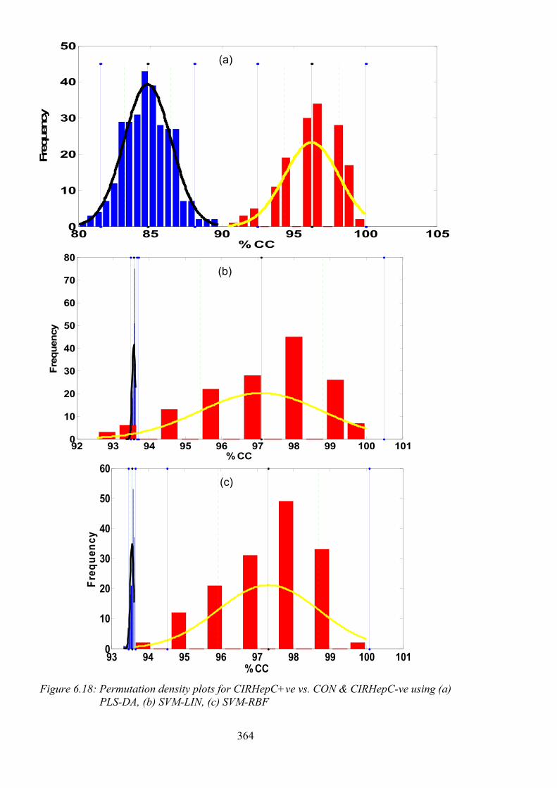
364

Figure 6.18: Permutation density plots for CIRHepC+ve vs. CON & CIRHepC-ve using (a)

PLS-DA, (b) SVM-LIN, (c) SVM-RBF

80 85 90 95 100 1050

10

20

30

40

50

% CC

Freq

uenc

y;

92 93 94 95 96 97 98 99 100 1010

10

20

30

40

50

60

70

80

% CC

Freq

uenc

y

93 94 95 96 97 98 99 100 1010

10

20

30

40

50

60

% CC

Freq

uenc

y

(a)

(b)

(c)

365

Figure 6.19: Permutation density plots for CIRHepC+ve vs. CON & CIRHepC-ve using

ANNs with PNNs (a) without feature selection, (b) with feature selection.

Balanced data set

Because of the biased results discussed, a smaller, balanced number of controls (CON &

CIRHepC-ve) were used in the classification against CIRHepC+ve. The results for the mean

of the classification models when using the classifiers, PLS-DA, SVM and ANNs, with and

without feature selection, can be seen in Table 6-13.

For all three classifiers, feature selection through the Wilcoxon t-test with p=0.05 gave the

best results, with ANNs consistently producing the highest performance for all monitors,

85 90 95 100 1050

10

20

30

40

50

% CC

Freq

uenc

y

85 90 95 100 1050

10

20

30

40

50

% CC

Freq

uenc

y

(a)

(b)

366

except specificity, where SVM-RBF was slightly better. SVM-RBF gave a much higher

performance than SVM-LIN.

Table 6-13: CIRHepC+ve vs. balanced CON & CIRHepC-ve using PLS-DA, SVM and ANNs


Feature selection

None WTT p=0.05

None WTT p=0.05

None WTT p=0.05

None WTT p=0.05

No. scans 8701 290 8701 290 8701 290 8701 290

Scaling None Norm MC Norm AS AS Norm RS (0 to 1)

%CC 70.87 73.00 60.13 63.53 65.47 74.6 59.93 82.8

%Spec 60.13 61.20 56.53 56.93 75.87 75.87 100.00 73.33

%Sens 81.60 84.80 63.73 70.13 55.07 73.33 19.87 92.27

%NPV 78.11 81.53 67.09 70.16 66.48 77.09 55.94 92.91

%PPV 69.27 70.02 57.88 61.55 63.56 72.75 72.00 79.56

%FDR 30.73 29.98 42.12 38.45 36.44 27.25 28.00 20.44

LV 11 2

AUROC 0.8325 0.8564 0.6245 0.6967 0.5056 0.8383 0.5993 0.9501

The permutation density plots for the three best classifiers of the balanced data sets is shown

in Figure 6.20. As before, the performance data from the mean of the models shown in the

table, does not completely reflect the performance when comparing against the null models.

When the full control data set was used, the mean of the null models was 85 % or higher,

showing considerable bias. For the balanced data sets, the mean of the null models is where

they should be, centred on 50% CC.

367

Figure 6.20: Permutation density plots for CIRHepC+ve vs. balanced CON & CIRHepC-ve

using (a) PLS-DA, (b) SVM-RBF, (c) ANNs

30 40 50 60 70 80 90 100 1100

5

10

15

20

25

30

35

40

45

% CC

Freq

uenc

y

40 50 60 70 80 90 100 1100

20

40

60

80

100

120

% CC

Freq

uenc

y

;

30 40 50 60 70 80 90 100 1100

10

20

30

40

50

% CC

Freq

uenc

y

;

(a)

(b)

(c)

368

The distribution of the null models for PLS-DA and ANNs is very similar and quite broad,

with a few models over 75 %, whereas the SVM-RBF is much narrower, but still has a null

model at 70 %. The distribution of the sample classification models is similar for all three

classifiers, with the worst performing models around 40% and the best near 100 %.

However, the mean is better for ANNs than the other classifiers. Although there is no

complete separation of all models, each classifier produced separation of the mean null and

mean analysis models at greater than two STDDEV. Visually, ANNs is still the best

performing classifier.

The only way to improve the density plots, is to acquire more CIRHepC+ve samples to

compare against the control samples. This will enable more sample models to be generated

and hopefully narrow the distributions seen while maintaining or improving further the mean

of and the top performing models.

6.3 Studies by other groups, since this project

VOCs in the breath have also been studied pre- and post-liver transplant (Fernández del Río,

et al., 2015). First, the alveolar breath from 31 patients with liver cirrhosis and 30 healthy

controls was analysed by proton transfer reaction-MS (PTR-MS). PTR-MS is used for the

real-time monitoring of volatile compounds without any sample preparation or separation.

The neutral molecules in the breath are ionised through chemical ionisation by reacting with

protonated water before separating the ion by quadrupole-MS (qMS) or time-of-flight-MS

(ToFMS). In this study qMS was used and statistical techniques were used to compare the

data. Seven volatiles were found to be at higher concentrations in the liver cirrhosis patients.

The breaths of 12 of these patients were then analysed after having liver transplants. Five

of the previously observed raised volatiles had reduced significantly between pre-transplant

and post-transplant, with three of these volatiles resulting in an area under a receiver

369

operating characteristic curve (AUROC) of 0.95, a sensitivity of 97 % and a specificity of

70 %. On comparing the VOCs identified by Van den Velde (van den Velde, et al., 2008)

and Fernandez del Rio (Fernández del Río, et al., 2015), three of the four volatiles identified

in the early study were in the seven volatiles identified in the pre-transplant study by

Fernandez del Rio and colleagues. However, only one, 2-pentanone, was in the group of

three significant VOCs identified post-transplant.

Also, the analysis of plasma samples by GC-MS has been revisited (Nezami Ranjbar, et al.,

2015). The plasma from 40 hepatocellular carcinoma (HCC) patients and 49 patients with

liver cirrhosis were analysed by derivatisation using MSTFA followed by GC-qMS and GC-

ToFMS analysis. Metabolites were identified by metabolomics libraries and statistical

analysis using two-way analysis of variance (ANOVA) models to select those metabolites

with the highest statistical differences, resulting in nine potential biomarkers for HCC with

false discovery rate (FDR) values of <10 %. In a similar study, serum was analysed from

49 HBV, 52 liver cirrhosis (LC), 39 HCC and 61 healthy non-cancer (NC) patients by

derivatisation with MSTFA followed by GC-ToFMS analysis (Gao, et al., 2015). The data

was then analysed using PCA, PLS-DA, RFs and HCA to identify possible metabolites.

Binary logistic regression of the validation sets gave a classification sensitivity of 100 % and

specificity of 95.2 % for HBV vs. NC. A sensitivity of 83.3 % and specificity of 100 % for

LC vs. HBV. A sensitivity of 76.9 % and specificity of 83.3 % for HCC vs. LC. Combined,

the classification accuracies were 100 % for NC, 94.12 % for HBV, 100 % for LC and 76.92

% for HCC. The focus of these studies was the identification of biomarkers for these

different hepatic disorders.

The focus of these publications has been the sensitivity and specificity, when from previous

discussions the performance monitors should also be focussed on the %PPV and %NPV for

the clinicians along with the AUROC value. None of the publications mention permutation

370

testing which, from our studies, is very important to determine how significant the results

really are.

6.4 Summary and future work

The results for the hepatic disorders study look even more promising than the two previous

studies for bladder and prostate cancers. We could differentiate between those with liver

cirrhosis and various other illnesses with all performance monitors of 86 % or greater and a

‘very good’ AUROC score using PLS-DA, which is very similar to other publications.

However, the excellent results from the permutation testing underlines the significance and

lack of bias of the models generated by our analyses.

The ability to differentiate between those with liver cirrhosis caused by HCV and non-HCV

cirrhosis combined with controls, also looks promising, but far more data is required.

Biomarker identification on the current data sets, by using the PLS loadings plot to determine

retention times of potential biomarkers and then performing library searching on their mass

spectra needs to be performed. These can then be compared to potential biomarkers

published by other groups.

Urine samples are easier to collect, transport and store than breath samples, therefore the

possibility to identify not only liver cirrhosis but the source of that cirrhosis, particularly for

HCV would be very beneficial.

371

Classification of the Septic Infection of

Intensive Care Patients

372

7.1 Introduction

Although many of the methods investigated over the past 30 years for the diagnosis of

bacteria have not made it into the routine lab environment, much of the research was carried

out using less sensitive instrumentation unable to detect, analyse and identify compounds

like we can today. Chemometric techniques, for pattern recognition in complex and large

data sets, were either not available, or were in their earlier stages of development. The

widely-reported potential of HS-GC techniques for identification of bacterial infections, fits

well with the methods developed in this thesis. It was also appropriate to explore the

application of TD as an alternative sampling methodology to HS-SPME. Therefore, it is

well worth revisiting this area, especially considering the development of the sample analysis

techniques performed for bladder and prostate cancers and hepatic disorders studies, as well

as the chemometric techniques by Dr Michael Cauchi of Cranfield University.

It was hypothesised that analysis of the headspace above bacterial cultures by GC-ToFMS

would provide plenty of data to be analysed using chemometric techniques, which we hoped

would at least confirm the presence or absence of bacteria and hopefully identify the type of

bacteria the patient is infected with. Further investigation for the identification of specific

biomarkers would be advantageous too.

7.1.1 Proof of concept

A proof of concept was carried out to determine if this project was worth pursuing. Although

protocols are in place to analyse urine samples in the department, the research into

microbiology samples involved the analysis of the headspace above blood cultures.

Therefore, considering Health & Safety in addition to practical sampling collection and

analysis, we decided to analyse some samples, containing a variety of bacteria, in-situ in the

labs of our project partners, Dr Kevin Fong and Dr Tom Bashford, at University College

373

London Hospital (UCLH), London. The headspace of the blood cultures could be sampled

using the following techniques:

• HS analysis: this sample had to be taken from the sample bottle and injected straight

into the GC-MS. A GC-MS instrument was used in the Biochemistry Department at

UCLH, but the sampling had to be carried out manually, as a HS autosampler wasn’t

available.

• TD analysis: UCLH didn’t have the equipment to perform TD analysis in their labs,

so the headspace was: sampled onto a clean TD tube and sealed; heated to kill any

possible bacteria drawn onto the tube; and taken back to The Open University for

analysis by GC-MS. One batch (10 tubes) was purchased for the study.

• SPME analysis: UCLH didn’t have the equipment to perform this in their labs;

manual sampling would take a long time with a single SPME fibre; the main problem

was the possible exposure to bacteria. Therefore, we decided not to investigate this

technique during the preliminary study.

Risk assessments were carried out for the analysis of the blood cultures using the two

techniques applied.

The objectives of the preliminary study were to:

• Analyse as many samples using the two techniques in the one day available.

• Observe any differences in the profile of VOCs in the headspace between blank

aerobic and anaerobic bottles plus and cultured bacteria samples.

• Observe any differences between the different types of bacteria.

• Determine which method was better: HS or TD.

374

7.1.2 Sample recruitment

Samples were obtained from the Microbiology Department at UCLH. Prior to analysis it

was unknown which bacteria, or how many of each type, would be present in any sample on

any one day. Therefore, it was very much a matter of luck if there would be enough samples

giving a positive reading in their BACTECTM system on that or the previous day.

Microbiologists on the day and the day before the preliminary study, on confirmation of a

positive result kept samples in the incubator ready for collection. As it can take 1-2 days for

the gram stain and subculture to identify the bacterium present, the HS-GC-MS samples

were analysed blind.

Anaerobic and Aerobic BACTECTM bottles containing positive samples that had been

cultured and identified at UCLH were analysed.

7.1.3 Study samples and analysis methods

7.1.3.1 Samples and HS-GC-MS method

There were three different types of bacteria that were analysed by HS-GC-MS following the

method described in Section 2.3.2.2. The bacteria were identified as:

• Escherichia coli (E. coli)

• Coagulase-negative Staphylococcus (Coag. neg. staph.)

• Staphylococcus aureus and alpha-haemolytic streptococcus (Staph. aureus & Alpha

haem. strept.)

The number of samples analysed from Aerobic and Anaerobic BACTECTM bottles

containing different bacteria are summarised in Table 7-1.

375

Table 7-1: Summary of number of samples of each type analysed by HS-GC-MS

Blank or bacteria type Aerobic bottles Anaerobic bottles

E. coli 3 2

Coag. neg. staph 0 2

Staph. aureus & Alpha haem. strept. 1 1

Failed to grow by GPC 0 1

Blank bottle 2 2

The samples, data file names and conditions used in the figures are summarised in Table 7-2.

As is shown, the samples were analysed randomly (bacteria type unknown) with blanks

interspersed, including syringe blanks (SyrBlk) of air and BACTECTM bottle blanks (Blank

or Blk).

The method was being developed as the samples were injected, hence the variations in the

incubation temperature, time and split ratio while sampling. All samples had been incubated

at 37 °C before being taken to the lab in an insulated bag for analysis.

After injection of the first sample very few peaks were seen. It was unknown at the time

that this sample had also failed to grow by gel-permeation chromatography (GPC), meaning

that there might not have been any bacteria present in the bottle. Based on the assumption

that the cultured bacteria should have been present, the split ratio was reduced from 10:1 to

5:1 to improve the sensitivity. The temperature was also changed throughout the process

from the majority being analysed at room temperature, then incubation at 37 °C and finally

56 °C to see if more volatiles analytes could be sampled.

376

Table 7-2: Summary of samples and conditions in the analysis by HS-GC-MS

Inj. no. Data file name Bacteria type Bottle Type

Inc. T (°C)

Inc. time (hr)

Split ratio

2 SyrBlk1 None NA NA NA 10:1

8 SyrBlk2 None NA NA NA 5:1

10 Blank_Aerobic None Aerobic Room T 0 5:1

14 Blk_A_Hot None Aerobic 37 1.5 5:1

5 X576_A E. coli Aerobic Room T 0 5:1

11 H38707_Aerobic E. coli Aerobic 37 3 5:1

15 M41244_A_56 E. coli Aerobic 56 1 5:1

4 X13_A Staph. aureus + alpha haem. strept.

Aerobic Room T 0 5:1

7 Blank_An None Anaerobic Room T 0 5:1

13 Blk_An_Hot None Anaerobic 37 2.25 5:1

12 H38707_An E. coli Anaerobic 37 3.25 5:1

16 M42051_An E. coli Anaerobic 56 1.25 5:1

6 X12_An Coag neg. staph. Anaerobic 37 1 5:1

9 S12805_An Coag neg. staph. Anaerobic 37 2 5:1

3 X13_An Staph. aureus + alpha haem. strept.

Anaerobic Room T 0 5:1

1 T64012_An GPC - failed to grow

Anaerobic Room T 0 10:1

Shows Injection number (Inj. no.), incubation temperature (Inc. T) and time (Inc. time), inlet

split ratio (split ratio).

7.1.3.2 Samples analysed by TD-GC-MS

There were six different types of bacteria analysed by TD-GC-MS, following the method

described in Section 2.3.3.3.

• Escherichia coli (E. coli)

• Coagulase-negative staphylococcus (Coag. neg. staph.)

• Staphylococcus aureus and Alpha-haemolytic streptococcus (Staph. aureus & Alpha

haem. strept.)

377

• Microcococcus species (Micrococcus spp.)

• Klebsiella pneumoniae

• Vancomycin-resistant enterococci (Vanc. resistant enterococcus)

The number of samples analysed from Aerobic and Anaerobic BACTECTM bottles,

containing the different bacteria, are summarised in Table 7-3.

Table 7-3: Summary of number of samples of each type analysed by TD-GC-MS

Blank or bacteria type Aerobic bottles Anaerobic bottles

E. coli 1 1

Coag. neg. staph 1 0

Micrococcus spp. 1 0

Staph. aureus & Alpha haem. strept. 1 1

Klebsiella pneumoniae 1 1

Vanc. resistant enterococcus 0 1

Failed to grow by GPC 0 0

Blank bottle 1 1

A summary of the samples and their analysis conditions are given in Table 7-4.

Unfortunately, no replicates for each of the bacteria types, in each of bottles, were available

for comparison.

The instrument was checked for contamination by analysing two instrument blanks

(TD_GCMS_Blk), where the TD trap was fired and the GC-MS acquired the data files. After

the first sample (Injection 3) was analysed, the TD tube that had been used was re-analysed

two further times to check for carryover (Injections 4 and 5). No carryover was seen and

therefore the remainder of the samples were analysed randomly. The TD tube used for

Injection 10 was again re-analysed (Injections 11 & 12) to confirm the previous findings.

378

Table 7-4: Summary of samples and conditions in the analysis by TD-GC-MS.

Inj. No. Data file name Bacteria type Bottle Inc. T (°C) Inc. time (hr) Static HS Dynamic HS Used for HS? 1 TD_GCMS_Blk1 None NA NA NA NA NA NA 2 TD_GCMS_Blk2 None NA NA NA NA NA NA 4 Mi167821 None NA NA NA NA NA NA 5 Mi167821_2 None NA NA NA NA NA NA 11 Mi167822_1 None NA NA NA NA NA NA 12 Mi167822_2 None NA NA NA NA NA NA

18 TD_Blank_A None Aerobic Room temp. NA 10 10 Yes 14 TD_X576_A E. coli Aerobic 37 4.25 10 0 Yes 7 TD_F66318_A Coag neg staph Aerobic 37 2.75 10 10 No 8 TD_H39091_A Klebsiella pneumoniae Aerobic 37 3.25 10 10 No 10 TD_S12901_A Micrococcus spp Aerobic 37 4 10 0 No 16 TD_X13_A Staph aureus + alpha haem strept Aerobic 56 4.75 10 0 Yes

17 TD_Blank_An None Anaerobic Room temp. NA 10 10 Yes 6 TD_M41244_An E. coli Anaerobic 37 2.25 10 10 No 9 TD_H39091_An Klebsiella pneumoniae Anaerobic 37 3.75 10 0 No 15 TD_X13_An Staph aureus + alpha haem strept Anaerobic 56 4.5 10 0 Yes 3 TD_X583_An Vanc resistant Enterococcus Anaerobic 37 2 10 10 No 13 TD_T64012_An GPC - failed to grow Anaerobic 37 4 10 0 Yes

Shows: Injection number (Inj. no.), bottle type (Bottle), incubation temperature (Inc. T) and time (Inc. time), how long the bottle was sampled under static and dynamic HS conditions; if the sample had previously been analysed by HS-GC-MS.

379

The method was also being developed further while sampling the sample bottles, therefore

some samples were sampled by:

• Static HS: where the static volume above the culture in the BACTECTM bottle was

sampled at 20 mL/min for 10 minutes.

• Dynamic HS: with 10 minutes of static HS followed by 10 minutes of dynamic HS,

where the second needle was inserted to draw air through the bottle.

Full details for both methods were provided in Chapters 2 and 3. Due to the limited

availability of samples, some samples collected onto a TD tube had been previously analysed

by HS-GC-MS.


The results and discussion are divided into three sections:

• The performance of the HS-GC-MS analysis will be discussed in Section 7.2.1, with

data analysis performed using NIST AMDIS software. There were no spectral

libraries present in the Shimadzu software and the data files could not be used with

Agilent software.

• The performance of the TD-GC-MS method will be discussed in Section 7.2.2, with

data analysis performed using Agilent MSD Chemstation software.

• Chemometric analysis of both data sets by Cranfield University will be discussed and

compared in Section 7.2.3.

7.2.1 HS-GC-MS data

There weren’t many samples to compare or data to generate performance data as this was

conceived as a proof of concept study. Contractual issues prevented the larger follow-on

380

study from taking place. However, blanks were assessed and sample chromatograms

compared and discussed in this section.

7.2.1.1 Method performance: blanks

The syringe blank data file was analysed and along with the air peak the solvents acetone,

ethanol, n-hexane and cyclohexane were identified, plus some small siloxane peaks. On

comparison with the aerobic and anaerobic blank bottles, no additional peaks were identified

in the aerobic blank bottle except for larger siloxane peaks and ethanol peaks. In the

anaerobic blank bottle, 1,3-dimethyl benzene and methyl-cyclopentane were also identified.

The chromatograms are shown in Figure 7.1.

Figure 7.1: TICs of HS-GC-MS blanks (a) syringe; (b) aerobic bottle; (c) anaerobic bottle

381

7.2.1.2 Sample bottles

As shown in Figure 7.2, when comparing the aerobic samples to the aerobic blank there was

very little difference in the chromatograms. Even when using deconvolution, except for

siloxane peaks, the only additional peak seen and identified was acetic acid, present in the

Staph. aureus + alpha haem. strept. sample, with a smaller peak present in an E. coli sample.

On comparison of the anaerobic samples to the anaerobic blank, again there were no

significant differences seen, with only slight variations in the solvents and siloxane peaks

previously discussed for the anaerobic bottle.

Figure 7.2: TICs of HS-GC-MS (a) aerobic blank; (b) aerobic Staph. aureus + alpha haem.

strept.

Overall, the HS-GC-MS method showed very poor sensitivity, with very few peaks seen in

the chromatograms or extracted using deconvolution.

382

7.2.2 TD-GC-MS data

7.2.2.1 Method performance: blanks

Manual comparisons and peak identification was made using the instrument software.

Chromatograms comparing an instrument blank with a TD tube blank, aerobic and anaerobic

bottle blanks are shown in Figure 7.3.

Background from the instrument was very low, with only a couple of peaks identified as

siloxanes and sulphur dioxide, most likely to be artefacts from the TD cold trap sorbent.

Analysis of a conditioned TD tube produced the same siloxanes and sulphur dioxide at a

higher abundance, plus the extra peaks: benzene and styrene, which are known artefacts of

the TD tube sorbents.

On the analysis of the blank aerobic and anaerobic BACTECTM bottles, with no sample only

the culture medium, the background was much higher. This is to be expected, as all tubing

used in the sampling system, the bottle itself (including septum and the medium) will

produce volatiles. For example, both ethanol and acetone were analysed from the culture

medium, multiple branched and cyclic hydrocarbons from either the medium or the sampling

parts, low level phthalates and plasticisers from the tubing and bottle septum. Comparing

the aerobic and anaerobic bottle chromatograms, the peaks were identified as being the same

compounds, they were just present at different concentrations.

Future work, in a larger scale project, would need to include the analysis of multiple blank

bottles and a comparison between the sample bottles themselves and those bottles that do

not contain medium, to see how consistent the background signal is.

383

Figure 7.3: Comparison of Anaerobic (red) and Aerobic (blue) bottle blanks against instrument (black) and TD tube (green) blanks

7.2.2.2 Method performance: carryover

After the first sample (Vanc. resistant enterococcus from the anaerobic bottle) was analysed,

the same TD tube was analysed twice more. This was to determine if there had been any

carryover. If in the first desorption, all the analytes from the TD tube had not been fully

desorbed, or the system had been left contaminated after sample analysis, peaks would still

384

be present on the second desorption of the TD tube. The third desorption would then show

fewer peaks again at lower abundancies. Carryover was checked for, before the remaining

samples were analysed. The chromatograms from the sample and subsequent desorptions

of the TD tube are shown in Figure 7.4. The second blank desorption chromatogram was

already compared to an instrument blank and BACTECTM bottle blanks in Figure 7.3.

Comparing the chromatogram of the sample against the two TD tube blanks, there were

many large peaks in the sample chromatogram and very few peaks in the TD tube blanks.

The peaks present in the TD tube blank were also much lower in abundance. Comparing the

chromatograms of the two TD blank analyses, they are very similar in terms of the number

of peaks and the abundances of those peaks. The three chromatograms were integrated using

the real-time execution (RTE) integrator and the results determine for all peaks present in all

three chromatograms are presented in Table 7-5.

The percentage carryover was calculated by comparing the peak areas from the first blank

TD tube desorption against the areas of the same peaks from the sample analysis. The areas

of the first and second blank TD tube desorptions were then compared and presented, where

a value of 1 means the areas are comparable and 0.5 means the second desorption area is

half the size of the first desorption area. Many of the peaks from both desorptions were very

small, therefore the accuracy of integration, which was not optimised, may cause much of

the difference.

The TD tube blanks will never be completely peak-free, due to sorbent heating artefacts, as

discussed previously. Out of the 24 integrated peaks, nine had a carryover of < 1 %, a further

nine had a carryover of < 10 %.

The peak at 15.58 minutes, tentatively identified as styrene, had a consistent size in all three

analyses, indicating it must be an artefact of the method, rather than coming from a sample.

385

Figure 7.4: Carryover check for anaerobic bacteria

386

Table 7-5: Carryover peak data

Sample desorption 2nd desorption 3rd desorption Retention

Time (min)

Area (arbitrary

units)

Area (arbitrary

units) Carryover

(%)

Area (arbitrary

units)

Ratio of areas

3rd cf. 2nd Tentative

Identification

2.633 1758999 12342 0.70 8764 0.71 Argon

2.716 2918097 8024 0.27 3674 0.46 Carbon dioxide

3.37 3027708 692756 22.88 572099 0.83 Sulphur dioxide

3.805 1328062 74715 5.63 46284 0.62 Acetaldehyde

3.856 1322680 44578 3.37 33803 0.76 2-Butene

4.476 25388094 57794 0.23 24130 0.42 Ethanol

5.141 1069004 27987 2.62 21331 0.76 ?

5.27 7419961 33672 0.45 5027 0.15 Acetone

5.944 472322 4105 0.87 7576 1.85 Siloxane

6.618 7523368 42765 0.57 3773 0.09 Siloxane

9.015 1262945 5040 0.40 3968 0.79 ?

9.549 2256760 827250 36.66 658854 0.80 Benzene

10.034 196186 7870 4.01 0 0.00 ?

12.453 337902 81324 24.07 25736 0.32 Toluene

12.615 188026 12302 6.54 27773 2.26 ?

12.87 108093 9048 8.37 19195 2.12 Siloxane

13.137 230630868 2271622 0.98 1696316 0.75 Siloxane

14.793 2417202 63492 2.63 49472 0.78 Ethylbenzene

15.079 5838192 75523 1.29 34502 0.46 m-Xylene

15.577 179814 163417 90.88 145433 0.89 Styrene

15.687 1355468 32704 2.41 8880 0.27 o-Xylene

16.805 350686968 528199 0.15 387213 0.73 Siloxane

17.217 114170 19371 16.97 7820 0.40 Benzaldehyde

19.748 23454253 413114 1.76 314081 0.76 Siloxane

Two peaks, tentatively identified as sulphur dioxide and benzene, had an initial carryover on

the first desorption; however, on the second desorption the peak was approximately the same

size, again meaning that it was likely these compounds were artefacts.

Two peaks had carryover of 17-24 %, but then reduced again in size by 80 %. This cannot

be explained, however, after sampling the headspace from the bacterial culture bottles onto

the TD tubes, they were sealed with air inside and heated to 60 °C to kill any potential

387

bacteria present. This would potentially cause some damage to the sorbents due to oxidation

by the oxygen present and would explain some of these results.

For future work the damage to the tube on carrying out this process, needs to be investigated,

by conditioning and then analysing a clean TD tube. Sampling air onto the tube at the

flowrate and for the time described in the method. Sealing the tube and heating to the method

temperature for the method time. Then finally analysing the TD tube and comparing to the

first analysis.

On comparison of the second and third desorptions of the TD tube against the sample

desorption, it was deemed that there was negligible carryover caused by the sample analytes

and therefore the remainder of the samples were analysed as described in Section 2.3.3.2.

7.2.2.3 Aerobic sample compared to a blank aerobic bottle

A zoomed in chromatogram of an aerobic sample containing Klebsiella pneumoniae (black

trace) compared to a blank aerobic bottle (blue trace) is shown in Figure 7.5. The headspace

from the sample and blank bottles had both been extracted for a total of 20 minutes. The

blank bottle was incubated at room temperature, while the sample bottle was incubated at 37

°C. Many small peaks from the blank bottle were much larger from the sample bottle plus

there were many additional peaks. For example, the peak at 6.41 minutes was only present

in the sample trace and was identified through the RTL database as 1-propanol. Another

peak at 6.90 minutes was identified as MTBE and 3-methyl hexane at 9.64 minutes. The

peak at 4.87 minutes in the sample trace was not identified by the IARTL library. The mass

spectrum was therefore sent to the NIST library search algorithm and identified as 2-methyl

butane. Going back to the IARTL library this mass spectrum was not present and therefore

not identified as a target.

388

Figure 7.5: Zoomed in comparison of an aerobic sample vs. blank aerobic bottle by TD-GC-MS

389

Identification of the peaks against the retention time locked library means more certainty in

identification because retention time is used as a qualifier. A total of 55 target peaks were

automatically identified using this technique. However, manual comparison of these peaks

as well as the manual identification of peaks not identified by this limited library would be

very lengthy. Hence, it is much easier to do the comparison using chemometric techniques

which can also reveal hidden differences between the blanks and samples.

7.2.2.4 Comparison of all aerobic samples

An overlay of all five aerobic samples can be seen in Figure 7.6. As to be expected, in

general the two samples extracted for a total of 20 minutes showed higher abundances of

peaks than the three samples extracted for a total of 10 minutes. However, this was not the

case for all peaks, with the peak at 3.35 minutes showing a much higher concentration of

sulphur dioxide for Staph. aureus + Alpha haem. strept. (green trace) compared to other

samples. The 1,4-dioxane peak at 10.61 minutes was also higher for this sample. The Coag.

neg. staph. (blue trace) appeared to have the highest concentration of peaks.

7.2.2.5 Anaerobic sample compared to a blank aerobic bottle

A zoomed in chromatogram of an anaerobic sample containing E. coli (black trace)

compared to a blank anaerobic bottle (blue trace) is shown in Figure 7.7. The headspace

from the sample and blank bottles had both been extracted for a total of 20 minutes.

However, the blank bottle was incubated at room temperature, while the sample bottle was

incubated at 37 °C.

390

Figure 7.6: Zoomed in comparison of all aerobic samples by TD-GC-MS

391

Just as for the aerobic bottle comparisons, most small peaks from the blank bottle were much

larger from the sample bottle plus there were many additional peaks. For example, the peak

at 6.41 minutes was only present in the sample trace and was again identified through the

RTL database as 1-propanol. Other peaks identified were ethyl acetate (8.01 minutes), 1,1,1-

trichloroethane (9.01 minutes) and 1-butanol (9.09 minutes). All of them were identified

through deconvolution in the sample trace but not the bottle blank. Automatic deconvolution

and identification against the 171 compound IARTL library identified 58 targets, however

many of these were present in both sample and bottle blank.

7.2.2.6 Comparison of all anaerobic samples

An overlay of all five aerobic samples can be seen in Figure 7.8. In general, the two samples

extracted for a total of 20 minutes (black and red traces) showed higher concentrations of

peaks than the three samples (yellow, green and blue traces) extracted for a total of 10

minutes. This is to be expected. However, this was not the case for all peaks, the peak at

4.15 minutes, identified by IARTL as methanethiol, was only present in the Klebsiella

pneumoniae (blue trace) and E. coli (red trace) samples. The peak at 7.40 minutes, identified

by IARTL as possibly vinyl acetate, was only present in the Vanc resistant Enterococcus

(black trace) sample. 1-propanol, at 6.41 minutes was only detectable in the E. coli (red

trace) as a large peak and Klebsiella pneumoniae (blue trace) as a small peak. It was not

detected in the other three samples. The peak at 11.03 minutes was 3-methyl butanol, which

was present in all traces except for the GPC (failed to grow) data file.

Peaks from 14 minutes onwards, were much smaller with the small peaks barely detectable

for the samples that were extracted for 10 minutes rather than 20 minutes, showing the need

to optimise this part of the method in the future with real samples rather than just blank

aerobic and anaerobic bottles in the lab.

392

Figure 7.7: Zoomed in comparison of an anaerobic sample vs. blank anaerobic bottle by TD-GC-MS

393

Figure 7.8: Zoomed in comparison of all anaerobic samples by TD-GC-MS

394

As expected, the failed to grow by GPC sample (green trace) had by far the lowest number

and lowest abundances of peaks. The E. coli (red trace) appeared to have the highest number

and abundances of peaks.

7.2.3 Exploratory analysis by PCA and HCA

Data files were uploaded to the servers at Cranfield University, in .CSV format, in the future

NetCDF format will be used. Dr Michael Cauchi then processed them using chemometrics

techniques. There were not enough data files of any one type to perform supervised learning;

therefore, only exploratory analysis could be performed to look for any statistical differences

between the samples.

The TD-GC-MS data files had a total of ~14,900 scans, far more than the urine study samples

by HS-SPME-GC-ToFMS of ~8,700. This was due to the analysis time being longer, 28.5

compared to 15 minutes. However, the data files were treated in the same way as for the

urine analysis.

The blanks were treated as samples to determine if they could be differentiated from the

samples through natural groupings. There was no IS present for normalisation, but for future

work the TD autosampler has the possibility of using the automatic addition of an IS.

Usually toluene-d8 is used as it is volatile and not present in the samples. A TIC trace was

created by summing the abundances of the m/z, as previously described. The data files were

aligned using COW and no feature selection was performed. Multiple different scaling

methods were compared, including no scaling, mean-centre, auto-scale, range-scale (0 to 1),

range-scale (-1 to 1) and normalisation. HCA was performed using the Euclidean distance

and Ward linkage methods.

395

7.2.3.1 HS-GC-MS data

The first 150 scans were removed, as the air peak had a large influence on the data analysis,

producing no classification. Through implementing this method, discrimination improved

and gave similar results for no scaling, mean-centring and range-scaling (0 to 1). The PCA

plot with no scaling is shown in Figure 7.9. See Table 7-2 for the key to data file names.

Figure 7.9: PCA plot of the HS samples

88 % of the variance in the data set is captured in PC1, with a further 10 % in PC2. The

relationship between the samples can more clearly be seen from the HCA dendrogram in

Figure 7.10, with no scaling.

There is clearly a relationship between all the aerobic samples and the anaerobic samples,

except for the anaerobic blank. However, for some samples that are the same type, for

example the E. coli aerobic samples H38707 and M41244, they are more similar to the

blanks than they are to each other.

-6 -4 -2 0 2 4 6 8

x 105

-1

-0.5

0

0.5

1

1.5x 106

Blank_Aerobic

Blk_A_Hot

H38707_AerobicM41244_A_56

X13_AX576_A

Blank_AnBlk_An_Hot

H38707_An

M42051_An_56S12805_An

T64012_An

X12_An

X13_An

SyrBlk1

SyrBlk2

PC1 (88.3%)

PC

2 (9

.82%

)

PCA of Bacterial samples: HS

396

Figure 7.10: HCA dendrogram of the HS samples

7.2.3.2 TD-GC-MS data

The resultant PCA plot for the TD samples, with no scaling is shown in Figure 7.11. See

Table 7-4 for the key to data file names.

Figure 7.11: PCA analysis of data files from TD-GC-MS, no scaling

-2 -1 0 1 2 3 4 5

x 108

-1.5

-1

-0.5

0

0.5

1x 108

TD_Blank_A.CSV

TD_F66318_A.CSV

TD_H39091_A.CSV

TD_S12901_A.CSVTD_X13_A.CSVTD_X576_A.CSV

TD_Blank_An.CSV

TD_H39091_An.CSV

TD_M41244_An

TD_T64012_An.CSV

TD_X13_An.CSV

TD_X583_An.CSV

Mi167821_1.CSVMi167821_2.CSVMi167822_1.CSVMi167822_2.CSVTD-GCMS_Blk1.CSVTD-GCMS_Blk2.CSV

PC1 (91.2%)

PC

2 (3

.87%

)

PCA of Bacterial samples: TD

397

91 % of the variance in the data is captured in PC1 and a further 4 % in PC2. From this plot,

there are no clear clusters of data. Any relationships between the samples is easier to

visualise from the HCA dendrogram, shown in Figure 7.12.

Figure 7.12: HCA dendrogram of the TD samples and blanks

The different types of samples: instrument blanks, aerobic and anaerobic samples are very

well clustered together. However, differences can be seen between the individual samples.

Unfortunately, there were no duplicates of any bacteria type in the same medium to see if

they clustered together, as they should.


Although the data set was small, the data analysis using chemometric techniques could

provide answers to the objectives of the pilot study:

• We could observe differences in the headspace between the blank aerobic and

anaerobic bottles using both HS and TD.

• We could observe differences between the different types of bacteria when using

TD-GC-MS.

398

• The TD method was far more sensitive than the HS method, showing far more

differences between the different types of blanks and bacteria and better clustering

of samples from blanks. The GC-MS method used also provided around four times

more scans, providing more data to see any patterns and differentiate between the

samples.

The next steps would be to:

• Seek ethical approval.

• Decide the key bacteria to focus on and the number of samples and blanks to analyse.

• Write protocols for sample collection, transportation and analysis.

• Optimise the TD sampling, desorption and GC-ToFMS analysis, including use of

automatic IS addition for normalisation.

• Optimise chemometric techniques and biomarker identification.

Unfortunately, this project could not be taken any further at the time, despite having secured

funding for the next study. More sensitive instrumentation TD-GC-ToFMS had been

organised with the manufacturer for the sample analysis, along with trained staff to regularly

sample the BACTECTM bottles over a four-month study. The plan for this work can be seen

in Figure 7.13 and Table 7-6. However, the material transfer agreement for the samples

could not be agreed upon between The OU and UCLH.

399

Monday Tuesday Wednesday Thursday Friday Saturday Sunday May-13

1 2 3 4 5 Sample collection: UCLH

6 7 8 9 10 11 12 Sample analysis: ALMSCO

13 14 15 16 17 18 19 Data analysis/report writing: Cranfield

20 21 22 23 24 25 26 Finalise report: OU

27 28 29 30 31 Submit report: ISIC

Jun-13

1 2

3 4 5 6 7 8 9

10 11 12 13 14 15 16

17 18 19 20 21 22 23

24 25 26 27 28 29 30

Jul-13 1 2 3 4 5 6 7

8 9 10 11 12 13 14

15 16 17 18 19 20 21

22 23 24 25 26 27 28

29 30 31

Jul-13

1 2 3 4

5 6 7 8 9 10 11

12 13 14 15 16 17 18

19 20 21 22 23 24 25

26 27 28 29 30 31

Figure 7.13: Timetable for follow-on sepsis study

400

Table 7-6: Plan for follow-on sepsis study

End of: Max. no. TD tubes Max. no. samples Min. no. samples

Week 1 Extract up to 40 samples including max. of 5 no-grows 40 40 15


Week 3 Extract up to 40 samples including max. of 5 no-grows & ship to ALMSCO 120 120 45

Week 4 120 samples analysed by ALMSCO, tubes reconditioned & shipped back 160

Extract up to 40 samples including max. of 5 no-grows 40 160 60











Week 13 120 samples analysed by ALMSCO, tubes reconditioned & shipped back

Notes: Up to 40 collected per week - a mixture of bacteria and no-grows (control max. 5 per week)

At end of each week all samples headspace is extracted onto TD tubes = max. 40 tubes needed

After 3rd extraction all tubes are sent to ALMSCO for analysis, reconditioned and returned, meanwhile spare set of tubes are used

401

Conclusions and future work

402

The aim of the thesis was to develop and evaluate the performance of non-invasive methods

to characterise the disease states of patients utilising selective discrimination, gas

chromatography-mass spectrometry and chemometrics.

The primary analytical method that was investigated was gas chromatography-time-of-flight

mass spectrometry coupled with headspace solid-phase microextraction (HS-SPME-GC-

ToFMS); in addition, comprehensive gas chromatography (GCxGC) was also evaluated, as

were headspace (HS) and thermal desorption (TD) sampling techniques.

The main studies reported evaluations of the profiles of the headspace above urine samples

to classify the presence or absence of disease, as had previously been demonstrated by dogs.

Nearly 1,000 volatile organic compounds (VOCs) were observed using 1D GC and over

3,000 VOCs using GCxGC techniques. However, the inability to process the large GCxGC

data files restricted the use of the latter technique.

Therefore, the main focus of the method development, in Chapter 3, was on HS-SPME-GC-

ToFMS. A robust and sensitive method was developed by optimisation of all sample

analysis parameters. Its application for clinical samples was demonstrated through Chapters

4, 5 and 6, where the optimised method was evaluated for its suitability for detecting patients

with bladder cancer, prostate cancer and hepatic disorders.

The performance of the analytical method was assessed to determine if it was reproducible

and sensitive enough to enable classification of the different types of clinical samples. It

was shown that the differences in the analytes detected were due to the differences in the

clinical status of the sample, rather than any instrument and/or sample analysis error. This

evidence was obtained by quantifying the IS present in every sample and sample blank and

through the comparison of replicate samples in each study.

To summarise, the following conclusions were drawn about the method developed and

applied:

403

• The analysis of replicate samples, with consecutive and non-consecutive injections

in a batch and between-batch replicates showed no reduction in performance between

these types of replicates.

• The variability seen was not systematic, it was random, even over long periods and

so was likely to be due to errors in placing the collected sample into the vial, sample

preparation or extraction and injection.

• The variation in the response of the unknown analytes in the replicate injections

matched the IS response variation and therefore normalisation against the chosen IS

was possible.

• Assessing the library similarity match of the IS enabled an assessment of the

sensitivity of the method, alongside the IS peak areas and SN ratio.

Based on these findings, this analytical method was used to explore clinical samples with

confidence. A recommendation, for all future work, is that normalisation of the data against

the IS is necessary and highly recommended:

• To align the retention times, thus enabling comparison of the peaks in each data file

based on their scan number.

• To compare the response of the peaks in each data file more accurately, leading to

the generation of more significant classification results.

Further improvements to the sample analysis method, developed in this thesis, would

include:

• Using a well-characterised urine sample as a system suitability check before the start

of each batch. This would ensure the new SPME fibre is functioning properly as well

as checking the sensitivity of the whole GC-MS across the full volatility range, rather

than relying on just the single IS.

404

• Looking into more automated preparation of the internal standard. The latest CTC

autosampler enables the automatic changing of the syringe. This would enable

automatic addition of the IS prior to SPME analysis and could potentially improve

reproducibility over the manual method. However, the piercing of the vial septum

prior to pre-incubation, could potentially cause losses of some volatile analytes into

the vial septum, which would have to be investigated.

• The automatic addition of the acid solution and potentially a concentrated saline

solution, rather than solid sodium sulphate should be investigated, to automate the

sample preparation further and potentially reduce contamination. When to add these

in the process, for example as soon as the vials are loaded or as they are being

prepared; the effects of automation on the samples (and vial seals); as well as the

health and safety implications of the sample on the autosampler before it has been

neutralised; would all need to be investigated. Automation could improve

reproducibility in some ways, but reduce it in other ways.

Separate analytical methods were developed for the identification of the causative agents of

sepsis, from the profile of the volatile compounds present in the headspace above culture

samples, using HS-GC-MS and TD-GC-MS, as discussed in Chapter 7. Although the pilot

study was small, it was clear that the TD-GC-MS method provided better sensitivity.

Contractual issues curtailed the development and so future work should concentrate on

developing this method further with more samples and instrument time.

Mathematical models were then developed by Cranfield University for all four studies, to

determine if the diseased samples could be distinguished from the control samples, or in the

case of sepsis if the different bacteria could be distinguished from each other.

The classification results, for all three HS-SPME-GC-ToFMS studies, looked very

promising:

405

For bladder cancer, the comparison of most categories gave a mean accuracy of 80 % or

better using the PLS-DA classifier. For low grade tumours, C3 vs. TCC1 gave a sensitivity

of 73 % which is much better than 20- 50 % obtained when using the urine cytology.

The prostate cancer study produced very promising results, with even higher clinical

performance than the current gold standard diagnosis methods. Also, other benign

genitourinary tract diseases (e.g. BPH) did not affect the performance of the classifier and

classification of BPH against PC produced equally good performance, which has the

potential to be used for the differentiation of these two conditions that cause similar

symptoms. Discussions have begun with clinical partners to take this evaluation forward.

The results for the hepatic disorders study looked better still, with the ability to differentiate

between liver cirrhosis and various other illnesses with all performance monitors of 86 % or

greater and a ‘very good’ AUROC score using PLS-DA. Those with liver cirrhosis caused

by HCV could be differentiated from non-HCV cirrhosis and healthy controls; however, far

more data is required to fully validate the statistical significance of the findings.

Although only a very small study on sepsis was possible, differences between the different

types of bacteria when using TD-GC-MS were observed.

A large amount of high quality data was collected through these studies. However, I feel

that a large amount of this valuable information has still not been used. Further chemometric

analysis of the data should be focused on:

• Finding out which samples were classified as outliers and investigating the reasons

why they were classified as such. Potential reasons could be instrument acquisition

problems, IS concentration, or it could be related to the metadata from the

participants.

• Making more use of the metadata.

406

• Investigating if the specific gravity can be successfully used for normalising the urine

sample concentration.

• Using three-dimensional data for multivariate analysis rather than the two-

dimensional TIC data. This should be possible now, using the large amounts of high

quality data already generated, due to improvements in computing power since this

data was analysed.

• As all three urine studies used the same analysis method, classification of all these

samples together.

To be able to successfully classify and diagnose diseases and disorders, there are two parts

to the methodology:

Firstly, a robust, acquisition method to analyse the sample and to produce high quality

analytical data is required. This needs stringent quality control, using an IS, to check for

carryover and to correct for any drift in instrumentation and analyte extraction. Large,

balanced data sets are required to consider all differences between the samples and to

investigate the metadata, where age, smoking status, dipstick test results and even food and

drink intake may have an influence.

Secondly, experts in chemometric analysis techniques are required, to develop the data

processing methodology. Exploratory algorithms such as PCA and HCA didn’t reveal any

natural groupings and therefore pattern recognition techniques are required to train the

algorithms with known data sets, that need to be large enough to have statistical significance.

The scaling technique needs to be considered and assessed. Feature selection should be

considered, although it was generally deemed to be unsuitable, meaning that data reduction

generated poorer performing models. Bootstrapping, cross-validation and permutation

testing, using different classifiers and generating many classification models and null models

are necessary to thoroughly quantify the data and to make the results significant.

407

Finally, as much data as possible about the samples need to be acquired and used. For

example, dogs do not sniff individual compounds, they look at the whole profile. Putting

this into the laboratory means that all volatile compounds in the headspace above the sample

need to be extracted and analysed. Following on from this, all acquired data, with no data

reduction, needs to be used in statistical pattern recognition techniques, to obtain the best

classification of diseased vs. non-diseased samples with the highest accuracy and specificity.

Identification of potential biomarkers, reveals that there are many compounds, increasing or

decreasing in abundance throughout the whole analysis that contribute to the classification.

It would be good to identify, 1 or 10 or 50 biomarkers that enable the diagnosis of the disease,

but all evidence throughout these studies have revealed that although some compounds may

have more influence, they do not add up to most of the variance in the data and so the

comprehensive approach reported in this thesis is essential going forward.

409

Bibliography

Advisory Committee on Dangerous Pathogens, 2016. The Approved List of biological agents. misc208(rev3) ed. s.l.:Health and Safety Executive.

Aggio, R. B. M. et al., 2016. The use of a gas chromatography-sensor system combined with advanced statistical methods, towards the diagnosis of urological malignancies. Journal of Breath Research, 10(1), p. e017106.

Amal, H. et al., 2015. Detection of precancerous gastric lesions and gastric cancer through exhaled breath. BMJ, Volume 0, pp. 1-8.

Amal, H. et al., 2016. Breath testing as potential colorectal cancer screening tool. International Journal of Cancer, 138(1), pp. 229-236.

American Cancer Society, 2016. Can bladder cancer be found early?. [Online] Available at: http://www.cancer.org/cancer/bladdercancer/detailedguide/bladder-cancer-detection [Accessed 10 2016].

Bach, C., Dauchy, X., Chagnon, M.-C. & Etienne, S., 2012. Chemical migration in drinking water stored in polyethylene terephthalate (PET) bottles: a source of controversy. Water Research, 46(3), pp. 571-583.

Banez, L. L. et al., 2007. Obesity-related plasma hemodilution and PSA concentration among men with prostate cancer. Jama, 298(19), pp. 2275-80.

Barker, M. & Rayens, W., 2003. Partial least squares for discrimination. Journal of Chemometrics, 17(3), pp. 166-173.

Bassi, P. et al., 2005. Non-invasive diagnostic tests for bladder cancer: a review of the literature. Urologia Internationalis, 75(3), pp. 193-200.

Bawdon, D. et al., 2015. Identification of axillary Staphylococcus sp. involved in the production of the malodorous thioalcohol 3-methyl-3-sufanylhexan-1-ol. FEMS Microbiology Letters, 362(16), p. fnv111.

BBC News, 2016. Doctors name treatments that bring little or no benefit. [Online] Available at: http://www.bbc.co.uk/news/health-37732497 [Accessed 24 10 2016].

Brereton, R. G., 2007. Applied Chemometrics for Scientists. Chichester: Wiley.

Brereton, R. G., 2009. Chemometrics for Pattern Recognition. s.l.:Wiley.

Broadhurst, D. I. & Kell, D. B., 2006. Statistical strategies for avoiding false discoveries in metabolomics and related experiments. Metabolomics, 2(4), pp. 171-196.

Cancer Research UK, 2014. Bladder cancer statistics. [Online] Available at: http://www.cancerresearchuk.org/health-professional/cancer-statistics/statistics-by-cancer-type/bladder-cancer#heading-One [Accessed 10 2016].

Cancer Research UK, 2014. Liver cancer statistics. [Online] Available at: http://www.cancerresearchuk.org/health-professional/cancer-

410

statistics/statistics-by-cancer-type/liver-cancer#heading-Six [Accessed 10 2016].

Cancer Research UK, 2014. Prostate Cancer Statistics. [Online] Available at: http://www.cancerresearchuk.org/health-professional/cancer-statistics/statistics-by-cancer-type/prostate-cancer#heading-One [Accessed 10 2016].

Cancer Research UK, 2015. More about the stages of primary liver cancer. [Online] Available at: http://www.cancerresearchuk.org/about-cancer/type/liver-cancer/treatment/more-about-the-stages-of-primary-liver-cancer [Accessed 10 2016].

Cancer Research UK, 2015. The stages of primary liver cancer. [Online] Available at: http://www.cancerresearchuk.org/about-cancer/type/liver-cancer/treatment/the-stages-of-primary-liver-cancer [Accessed 10 2016].

Cauchi, M. et al., 2016. Evaluation of gas chromatography mass spectrometry and pattern recognition for the identification of bladder cancer from urine headspace. Analytical Methods, Volume 8, pp. 4037-4046.

Childs, S. & Williams, L., 2014. An Introduction into the Role of Gas Chromatography - Mass Spectrometry (GC-MS) in Metabolomic Analysis. Chromatography Today, February/March, pp. 3-4.

Cundy, K. V. et al., 1991. Comparison of traditional gas chromatography (GC), headspace GC, and the microbial identification library GC system for the identification of Clostridium difficile. Journal of Clinical Microbiology, 29(2), pp. 260-263.

Daniels, R., 2011. Surviving the first hours in sepsis: getting the basics right (an intensivist's perspective). Journal of Antimicrobial Chemotherapy, 66(2), pp. 11-23.

Dean, J. R., Tait, E., Stanforth, S. P. & Perry, J. D., 2014. Volatile Organic Compound Determination in Health-related Research: A Review. Chromatography Today, February/March, pp. 12-18.

Deans, D. R., 1968. A new technique for heart cutting in gas chromatography. Chromatographia, 1(1), pp. 18-22.

Di Natale, C. et al., 2005. Identification of schizophrenic patients by examination of body odor using gas chromatography-mass spectrometry and a cross-selective gas sensor array. Medical Science Monitor, 11(8), pp. CR366-75.

Ekelund, S., 2012. ROC Curves — What are They and How are They Used?. Point of Care: The Journal of Near-Patient Testing & Technology, 11(1), pp. 16-21.

Ettre, L. S., 1991. 1941–1951: The golden decade of chromatography. Analyst, Volume 116, pp. 1231-1235.

Fernández del Río, R. et al., 2015. Volatile biomarkers in breath associated with liver cirrhosis - comparisons of pre- and post-liver transplant breath samples. EBioMedicine, Volume 2, pp. 1243-1250.

411

Gao, R. et al., 2015. Serum metabolomics to identify the liver disease-specific biomarkers for the progression of hepatitis to hepatocellular carcinoma. Scientific Reports, Volume 5, p. 18175.

Glantz, S. A., 2005. Primer of Biostatistics. 6th ed. London: McGraw-Hill.

Glas, A. S. et al., 2003. Tumor markers in the diagnosis of primary bladder cancer. A systematic review. Journal of Urology, 169(6), pp. 1975-82.

Goldberg, E. M., Blendis, L. M. & Sandler , S. A., 1981. A gas chromatographic- mass spectrometric study of profiles of volatile metabolites in hepatic encephalopathy. Journal of Chromatography, Volume 226, pp. 291-299.

Goldstein, J. E. et al., 2013. Culture conditions and sample preparation methods affect spectrum quality and reproducibility during profiling of Staphylococcus aureus with matrix-assisted laser desorption/ionization time-of-flight mass spectrometry. Letters in Applied Microbiology, 57(2), pp. 144-50.

Goossens, H., Ferech, M., Van der Stichele , R. & Elseviers, M., 2005. Outpatient antibiotic use in Europe and association with resistance: a cross-national database study. Lancet, 365(9459), pp. 579-87.

Gootz, T. D., 2010. The global problem of antibiotic resistance. Critical Reviews in Immunology, 30(1), pp. 79-93.

Gopi, A. et al., 2011. Time to Positivity of Microorganisms with BACTEC 9050:- An 18-month Study Among Children of 28 Days to 60 Months in an South Indian Tertiary Hospital. International Journal of Microbiology Research, 2(1), pp. 12-17.

Grosch, W., 2001. Evaluation of the Key Odorants of Foods by Dilution Experiments, Aroma Models and Omission. Chemical Senses, Volume 26, pp. 533-545.

Guthery, B. et al., 2010. Qualitative drug analysis of hair extracts by comprehensive two-dimensional gas chromatography/time-of-flight mass spectrometry. Journal of Chromatography A, 1217(26), pp. 4402-10.

Haick, H. et al., 2014. Assessment, origin, and implementation of breath volatile cancer markers. Chemical Society Reviews, 43(5), pp. 1423-1449.

Hall, R. D. & Hardy, N. W., 2012. Practical applications of metabolomics in plant biology. Methods in Molecular Biology, Volume 860, pp. 1-10.

Hastie, T., Tibshirani, R. & Friedman, J., 2009. The Elements of Statistical Learning: Data Mining, Inference and Prediction. 2nd ed. New York: Springer.

Hilton, D., 2008. Analysis of Essential Oil Enantiomers by Chiral GCxGC-TOFMS, St Joseph, MI: Leco.

Hisamura, M., 1979. Quantitative analysis of methyl mercaptan and dimethyl sulfide in human expired alveolar gas and its clinical application: study in normal subjects and patients with liver diseases. Nippon Naika Gakkai Zasshi, Volume 68, pp. 1284-1292.

Horvath, I. et al., 2009. Exhaled biomarkers in lung cancer. European Respiratory Journal, Volume 34, pp. 261-275.

412

Ho, S. W., 1986. Head-space gas-liquid chromatographic analysis for presumptive identification of bacteria in blood cultures. Chinese Journal of Microbiology and Immunology, 19(1), pp. 18-26.

Huysmans, M. B. & Spicer, W. J., 1985. Assessment of head-space gas-liquid chromatography for the rapid detection of growth in blood culture. Journal of Chromatography, 337(2), pp. 223-9.

Immunization Action Coalition, p4075. Hepatitis A, B, and C: Learn the Differences, Saint Paul, Minnesota: http://www.immunize.org/.

Issaq, H. J. et al., 2008. Detection of human bladder cancer by LC-MS analysis of urine. Journal of Urology, 179(6), pp. 2422-2426.

Jentzmik, F. et al., 2010. Sarcosine in Urine after Digital Rectal Examination Fails as a Marker in Prostate Cancer Detection and Identification of Aggressive Tumours. European Urology, 58(5), pp. 12-18.

Julák, J., 2005. Chromatographic analysis in bacteriologic diagnostics of blood cultures, exudates, and bronchoalveolar lavages. Prague Medical Report, 106(2), pp. 175-94.

Julák, J., Stránská, E., Procházková-Francisci, E. & Rosová, V., 2000. Blood cultures evaluation by gas chromatography of volatile fatty acids. Medical Science Monitor, 6(3), pp. 605-10.

Kaji, H., Hisamura, M., Saito, N. & Murao, M., 1978. Evaluation of volatile sulfur compounds in the expired alveolar gas in patients with liver cirrhosis. Clinica Chimica Acta, Volume 85, pp. 279-284.

Khalid, T. et al., 2015. Urinary Volatile Organic Compounds for the Detection of Prostate Cancer. PLoS One, 10(11), p. e0143283.

Khalid, T. et al., 2013. A Pilot Study Combining a GC-Sensor Device with a Statistical Model for the Identification of Bladder Cancer from Urine Headspace. PLoS One, 8(7), p. e69602.

Kumar, S. et al., 2015. Mass Spectrometric Analysis of Exhaled Breath for the Identification of Volatile Organic Compound Biomarkers in Esophageal and Gastric Adenocarcinoma. Annals of Surgery, 262(6), pp. 921-90.

Kuntz, E. & Kuntz, H. D., 2008. Hepatology Textbook and Atlas. 3rd ed. s.l.:Springer.

Kusuhara, M., Urakami, K., Zangiacomi, V. & Hoshino, K., 2010. Disease and Smell "Byoshu". Anti-Aging Medicine, 7(6), pp. 66-72.

Lab Tests Online, 2015. ALT Test. [Online] Available at: http://labtestsonline.org.uk/understanding/analytes/alt/tab/test [Accessed 10 2016].

Lalkhen, A. G. & McCluskey, A., 2008. Clinical tests: sensitivity and specificity. Continuing Education in Anaesthesia, Critical Care and Pain, 8(6), pp. 221-223.

Larsson, L., Mardh, P. A. & Odham, G., 1978. Detection of Alcohols and Volatile Fatty Acids by Head-Space Gas Chromatography in Identification of Anaerobic Bacteria. Journal of Clinical Microbiology, 7(1), pp. 23-27.

413

Leotsakos, I. et al., 2014. Detection of Circulating Tumor Cells in Bladder Cancer Using Multiplex PCR Assays. Anticancer Research, Volume 34, pp. 7415-7424.

Lewis, V. R. et al., 2013. Researchers combat resurgence of bed bug in behavioral studies and monitor trials. California Agriculture, 67(3), pp. 172-178.

Liu, Z. & Phillips, J. B., 1991. Comprehensive Two-Dimensional Gas Chromatography using an On-Column Thermal Modulator Interface. Journal of Chromatographic Science, 29(6), pp. 227-231.

Lourenco, C. & Turner, C., 2014. Breath Analysis in Disease Diagnosis: Methodological Considerations and Applications. Metabolites, Volume 4, pp. 465-498.

Lozano, R. et al., 2012. Global and regional mortality from 235 causes of death for 20 age groups in 1990 and 2010: a systematic analysis for the Global Burden of Disease Study 2010. Lancet, Volume 380, pp. 2095-2128.

Maitra, S. & Yan, J., 2008. Principal Component Analysis and Partial Least Squares: Two Dimension Reduction Techniques for Regression. Discussion Paper Program, Casualty Actuarial Society.

Mardini, H. A. et al., 1987. Thermal desorption—gas chromatography of plasma isovaleraldehyde in hepatic encephalopathy in man. Clinica Chimica Acta, 165(1), pp. 61-71.

Markes International Ltd., 2012. Note 5: Advice on Sorbent Selection and Conditioning Sample Tubes, s.l.: Markes International Ltd..

Markes International Ltd., 2014. How to condition your sorbent tubes QQR-0287 Issue 1, s.l.: Markes International Ltd..

Marshall, A. W., DeSouza, M. & Morgan, M. Y., 1985. Plasma 3-methylbutanal in man and its relationship to hepatic encephalopathy. Clinical Physiology, Volume 5, pp. 53-62.

Mazzone, P. J., 2008. Analysis of volatile organic compounds in the exhaled breath for the diagnosis of lung cancer. Journal of Thoracic Oncology, 3(7), pp. 774-80.

Medscape, 2004. Manual of Laboratory & Diagnostic Tests. 7th ed. Philadelphia, Pa: Lippnicott, Williams & Wilkins.

Motulsky, H., 2010. Intuitive Biostatistics: A Nonmathematical Guide to Statistical Thinking. 2nd ed. Oxford: Oxford University Press.

Netzer, M. et al., 2009. A new ensemble-based algorithm for identifying breath gas marker candidates in liver disease using ion molecule reaction mass spectrometry. Bioinformatics, 25(7), pp. 941-7.

Nezami Ranjbar, M. R. et al., 2015. GC-MS Based Plasma Metabolomics for Identification of Candidate Biomarkers for Hepatocellular Carcinoma in Egyptian Cohort. PLoS One, 10(6), p. e0127299.

NHS Choices information, 2015. NHS choices. [Online] Available at: http://www.nhs.uk/Conditions/maple-syrup-urine-disease/Pages/Introduction.aspx [Accessed 09 2016].

414

NHS Choices, 2014. Haemochromatosis. [Online] Available at: http://www.nhs.uk/conditions/Haemochromatosis/Pages/Introduction.aspx [Accessed 10 2016].

NHS Choices, 2014. Liver disease. [Online] Available at: http://www.nhs.uk/conditions/liver-disease/Pages/Introduction.aspx [Accessed 10 2016].

NHS Choices, 2014. Primary biliary cirrhosis (primary biliary cholangitis). [Online] Available at: http://www.nhs.uk/conditions/Primary-biliary-cirrhosis/Pages/Introduction.aspx [Accessed 10 2016].

NHS Choices, 2015. Alcohol-related liver disease (ARLD). [Online] Available at: http://www.nhs.uk/conditions/Liver_disease_(alcoholic)/Pages/Introduction.aspx [Accessed 10 2016].

NHS Choices, 2015. Blood in urine (haematuria). [Online] Available at: http://www.nhs.uk/conditions/blood-in-urine/Pages/Introduction.aspx [Accessed 10 2016].

NHS Choices, 2015. Cirrhosis. [Online] Available at: http://www.nhs.uk/conditions/cirrhosis/Pages/Introduction.aspx [Accessed 10 2016].

NHS Choices, 2016. Hepatitis. [Online] Available at: http://www.nhs.uk/conditions/Hepatitis/Pages/Introduction.aspx [Accessed 10 2016].

NHS Choices, 2016. Liver cancer - diagnosis. [Online] Available at: http://www.nhs.uk/Conditions/Cancer-of-the-liver/Pages/Diagnosis.aspx [Accessed 10 2016].

NHS Choices, 2016. Non-alcoholic fatty liver disease (NAFLD). [Online] Available at: http://www.nhs.uk/Conditions/fatty-liver-disease/Pages/Introduction.aspx [Accessed 10 2016].

NHS Choices, 2016. Sepsis. [Online] Available at: http://www.nhs.uk/Conditions/Blood-poisoning/Pages/Introduction.aspx [Accessed 10 2016].

Niimura, Y. & Nei, M., 2006. Evolutionary dynamics of olfactory and other chemosensory receptor genes in vertebrates. Journal of Human Genetics, Volume 51, pp. 505-517.

Nitti, M., Pronzato, M. A., Marinari, U. M. & Domenicotti, C., 2008. PKC signaling in oxidative hepatic damage. Molecular Aspects of Medicine, 29(1-2), pp. 36-42.

Office for National Statistics, 2014. Cancer Registration Statistics, England: 2014. [Online] Available at: http://www.ons.gov.uk/peoplepopulationandcommunity/healthandsocialcare/conditionsanddiseases/bulletins/cancerregistrationstatisticsengland/2014 [Accessed 10 2016].

415

Otto, M., 2007. Chemometrics: Statistics and Computer Application in Analytical Chemistry. 2nd ed. Chichester: Wiley-VCH.

Parola, M. & Robino, G., 2001. Oxidative stress-related molecules and liver fibrosis. Journal of Hepatology, Volume 35, pp. 297-306.

Pasikanti, K. K. et al., 2010. Noninvasive Urinary Metabonomic Diagnosis of Human Bladder Cancer. Journal of Proteome Research, 9(6), pp. 2988-2995.

Pawliszyn, J., 2011. Handbook of Solid Phase Microextraction. s.l.:Elsevier.

Perez, A. et al., 2014. A Pilot Study on the Potential of RNA-Associated to Urinary Vesicles as a Suitable Non-Invasive Source for Diagnostic Purposes in Bladder Cancer. Cancers (Basel), 6(1), pp. 179-92.

PerkinElmer, Inc., 2014. An Introduction to Headspace Sampling in Gas Chromatography, s.l.: PerkinElmer, Inc..

Philips, M. et al., 2006. Prediction of breast cancer using volatile biomarkers in the breath. Breast Cancer Research and Treatment, Volume 99, pp. 19-21.

Phillips, M. et al., 1999. Variation in volatile organic compounds in the breath of normal humans. Journal of Chromatography B Biomedical Science Applications, 729(1-2), pp. 75-88.

Poulakis, V. et al., 2001. A comparison of urinary nuclear matrix protein-22 and bladder tumour antigen tests with voided urinary cytology in detecting and following bladder cancer: the prognostic value of false-positive results. BJU International, 88(7), pp. 692-701.

Probert, C. S. J. et al., 2009. Volatile Organic Compounds as Diagnostic Biomarkers in Gastrointestinal and Liver Diseases. Journal of Gastrointestinal Liver Diseases, 18(3), pp. 337-343.

RSC, 2016. Advances in Clinical Analysis 2016. [Online] Available at: http://www.rsc.org/events/detail/23842/advances-in-clinical-analysis-2016 [Accessed 2016].

Schiffer, E. et al., 2012. Urinary proteome analysis for prostate cancer diagnosis: cost-effective application in routine clinical practice in Germany. International Journal of Urology, 19(2), pp. 118-25.

Schulz, S. & Dickschat, J. S., 2007. Bacterial volatiles: the smell of small organisms. Natural Product Reports, 24(4), pp. 814-42.

Scotter, J. M. et al., 2006. The rapid evaluation of bacterial growth in blood cultures by selected ion flow tube-mass spectrometry (SIFT-MS) and comparison with the BacT/ALERT automated blood culture system. Journal of Microbiological Methods, 65(3), pp. 628-31.

Scott-Thomas, A. J. et al., 2010. 2-Aminoacetophenone as a potential breath biomarker for Pseudomonas aeruginosa in the cystic fibrosis lung. BMC Pulmonary Medicine, 10(1), p. 56.

Selley, S. et al., 1997. Diagnosis, management and screening of early localised prostate cancer. Health Technology Assessment, 1(2), pp. 1-96.

416

Shepherd, G. M., 2004. The human sense of smell: are we better than we think?. PLoS Biology, 2(5), p. e146.

Sigma-Aldrich, 2009. Selection Guide for Supelco SPME Fibers. [Online] Available at: http://www.sigmaaldrich.com/technical-documents/articles/analytical/selecting-spme-fibers.html [Accessed 10 2016].

Smith, D. & Spanel, P., 2015. SIFT-MS and FA-MS methods for ambient gas phase analysis: developments and applications in the UK. Analyst, Volume 140, pp. 2573-2591.

Smith, K., Thompson, G. & Koster, H., 1969. Sweat in Schizophrenic Patients: Identification of the Odorous Substance. Science, 166(3903), pp. 398-399.

Socolowsky, S., Höhne, C. & Sandow, D., 1990. The direct detection of volatile fatty acids by gas chromatography in microbiological diagnosis. Z Med Lab Diagn, 31(8), pp. 445-52.

Sreekumar, A. et al., 2009. Metabolomic profiles delineate potential role for sarcosine in prostate cancer progression. Nature, Volume 457, pp. 910-914.

SUPELCO, 1999. Solid Phase Microextraction Fiber Assemblies, Bellefonte, PA: Sigma-Aldrich Co..

Tait, E. et al., 2014. Development of a novel method for detection of Clostridium difficile using HS-SPME-GC-MS. Journal of Applied Microbiology, 116(4), pp. 1010-9.

Tangerman, A., Meuwese-Arends, M. T. & van Tongeren, J. H., 1983. A new sensitive assay for measuring volatile sulphur compounds in human breath by Tenax trapping and gas chromatography and its application in liver cirrhosis. Clinica Chimica Acta, Volume 130, pp. 103-110.

Thompson, I. M. et al., 2004. Prevalence of prostate cancer among men with a prostate-specific antigen level < or =4.0 ng per milliliter. New England Journal of Medicine, 350(22), pp. 2239-46.

Togneri, F. S. et al., 2016. Genomic complexity of urothelial bladder cancer revealed in urinary cfDNA. European Journal of Human Genetics, Volume 24, pp. 1167-1174.

Tomasi, G., van den Berg, F. & Andersson, C., 2004. Correlation optimized warping and dynamic time warping as preprocessing methods for chromatographic data. Journal of Chemometrics, 18(5), pp. 231-241.

Tsai, Y.-S.et al., 2015. Development of 3-Hydroxyanthranilic acid-based Integrated Non-invasive Biosensor for Bladder Cancer Detection. Urological Science, Volume 26, pp. S36-S49.

Turner, D. C., 2002. GCxGC-TOFMS and the Pegasus 4D for the Analysis of Pesticides in a Tobacco Extract, Cambridgeshire, UK: Anatune.

Ulanowska , A., Kowalkowski, T., Trawińska , E. & Buszewski , B., 2011. The application of statistical methods using VOCs to identify patients with lung cancer. Journal of Breath Research, 5(4), p. e046008.

Ulanowska, A. et al., 2011. Determination of volatile organic compounds in human breath for Helicobacter pylori detection by SPME-GC/MS. Biomedical Chromatography, Volume 3, pp. 391-7.

417

Ulanowska, A., Trawińska, E., Sawrycki , P. & Buszewski , B., 2012. Chemotherapy control by breath profile with application of SPME-GC/MS method. Journal of Separation Science, 35(21), pp. 2908-13.

Van Deemter, J. J. & Zuiderweg, F. J., 1956. Longitudinal diffusion and resistance to mass transfer as causes of nonideality in chromatography. Chemical Engineering Science, Volume 5, pp. 271-289.

van den Velde, S. et al., 2008. GC-MS analysis of breath odor compounds in liver patients. Journal of Chromatography B, 875(2), pp. 344-348.

Venkatesh, S. K., Yin, M. & Ehman, R. L., 2013. Magnetic Resonance Elastography of Liver: Technique, Analysis and Clinical Applications. Journal of Magnetic Resonance Imaging, 37(3), pp. 544-555.

Vitenberg, A. G. et al., 1986. Head-space gas chromatographic analysis in the rapid diagnosis of anaerobic infections. Zh Mikrobiol Epidemiol Immunobiol, Volume 1, pp. 20-24.

Watson, J. et al., 2007. Application of GCxGC-ToFMS in the analysis of meteoritic organic macromolecules. Torquay, 23rd International meeting on Organic Geochemistry.

Watt, B. et al., 1982. Can direct gas-liquid chromatography of clinical samples detect specific organisms?. Journal of Clinical Pathology, Volume 35, pp. 706-708.

Weber, C. M. et al., 2011. Evaluation of a gas sensor array and pattern recognition for the identification of bladder cancer from urine headspace. Analyst, 136(2), pp. 359-364.

Weckwerth, W., 2006. Metabolomics Methods and Protocols. s.l.:Humana Press.

Westerhuis, J. A. et al., 2008. Assessment of PLSDA cross validation. Metabolomics, 4(1), pp. 81-89.

Williams, H. & Pembroke, A., 1989. Sniffer dogs in the melanoma clinic?. Lancet, 1(8640), p. 734.

Willis, C. M. et al., 2004. Olfactory detection of human bladder cancer by dogs: proof of principle study. BMJ (Clinical Research ed.), 329(7468), pp. 712-714.

Wilson, A. D. & Baietto, M., 2011. Advances in Electronic-Nose Technologies Developed for Biomedical Applications. Sensors, Volume 11, pp. 1105-1176.

World Health Organisation, 2016. Hepatitis C. [Online] Available at: http://www.who.int/mediacentre/factsheets/fs164/en/ [Accessed 10 2016].

World Health Organization, 2014. World Cancer Report 2014, Lyon: edited by Bernard W. Stewart and Christopher P. Wild.

Wylie, P. L., Bates, M. & Woolfenden, E., 5989-5435EN. Screening for 171 Volatile Organic Air Pollutants Using GC/MS with Deconvolution Reporting Software and a New Indoor Air Toxics Library, s.l.: Agilent Technologies.

Xue, R. et al., 2008. Investigation of volatile biomarkers in liver cancer blood using solid-phase microextraction and gas chromatography/mass spectrometry. Rapid Communications in Mass Spectrometry, Volume 22, pp. 1181-1186.

418

Zhu, F.-Y.et al., 2007. Study on the Characteristic Components in the Human Urine with Bladder Cancer. Analytical Chemistry, 35(8), pp. 1132-1136.

419

Appendix A Publication

Evaluation of gas chromatography massspectrometry and pattern recognition for theidentification of bladder cancer from urineheadspace

M. Cauchi,*a C. M. Weber,a B. J. Bolt,a P. B. Spratt,a C. Bessant,b D. C. Turner,c

C. M. Willis,d L. E. Britton,d C. Turnerc and G. Morganc

Previous studies have indicated that volatile organic compounds specific to bladder cancer may exist in

urine headspace, raising the possibility that they may be of diagnostic value for this particular cancer. To

further examine this hypothesis, urine samples were collected from patients diagnosed with either

bladder cancer or a non-cancerous urological disease/infection, and from healthy volunteers, from

which the volatile metabolomes were analysed using gas chromatography mass spectrometry. The

acquired data were subjected to a specifically designed pattern recognition algorithm, involving cross-

model validation. The best diagnostic performance, achieved with independent test data provided by

healthy volunteers and bladder cancer patients, was 89% overall accuracy (90% sensitivity and 88%

specificity). Permutation tests showed that these were statistically significant, providing further evidence

of the potential for volatile biomarkers to form the basis of a non-invasive diagnostic technique.

Introduction

Bladder cancer is the seventh most common cancer in the UK,with over 10 700 new cases diagnosed in 2012.1 As with mostcancers, early diagnosis greatly increases the chances ofsurvival; individuals presenting with stage I tumours havinga one year relative survival rate of around 97%, compared to26% for those with stage IV disease.2 For people exhibitingsymptoms or requiring surveillance, cystoscopy with biopsyremains the “gold standard” investigative technique for bladdercancer detection, but is invasive, expensive and time-consuming. Urine cytology can be a useful non-invasive adjunctto diagnosis, since it has a high specicity for bladder cancer(96–98%), but its sensitivity is low (22–52%), especially for low-grade tumours which shed proportionally fewer cells into theurine. Furthermore, an experienced cytologist or pathologist isneeded to perform the cytological evaluation, making the testrelatively expensive and slow.3

Utilisation of molecular biomarkers present in urine offersa promising alternative non-invasive approach to diagnosis,

which if sufficiently accurate, rapid and cheap has the potentialto be used for mass screening of the population. Of the proteinmarkers which have so far been investigated in depth, threehave achieved FDA approval as assays for diagnosis and/orfollow-up – nuclear mitotic apparatus protein (NMP22),complement factor H-related protein and complement factor H(BTA stat® and BTA TRAK®), and carcinoembryonic antigencombined with two bladder tumour cell-associated mucins(ImmunoCyt™/uCyt+™).4,5 Whilst these are more sensitivethan urine cytology, having reported sensitivities of 47–100%,53–83% and 50–100%, respectively, specicities are signi-cantly lower at 60–90%, 51–75% and 69–79%, respectively.

Recently, it has been suggested that volatile organiccompounds (VOCs) present in the headspace of urine frombladder cancer sufferers may be used as diagnostic biomarkers.This concept was initially demonstrated in a canine olfactoryproof-of-principle study by Willis et al.6 and subsequently sup-ported by ndings using a metal oxide semiconductor (MOS)and eld effect transistor (MOSFET) gas sensor array,7 wheresensitivity and specicity rates of up to 70% were achieved. Amore recent pilot study by Khalid et al.8 involving 24 bladdercancer patients and 74 control patients with non-malignanturological disease, utilised an in-house fabricated combinedgas chromatography (GC) MOS-sensor device with patternrecognition, reporting accuracies of between 93% and 100% forthe correct assignment of urine samples. Although very prom-ising, the authors acknowledge that larger sample sizes areneeded to conrm the results.

aCraneld Biotechnology Centre, Craneld University, Bedfordshire, MK43 0AL, UK.

E-mail: [email protected] of Biological and Chemical Sciences, Queen Mary University of London, Mile

End Road, London E1 4NS, UKcDepartment of Life, Health and Chemical Sciences, Open University, Milton Keynes,

MK7 6AA, UKdDepartment of Dermatology, Amersham Hospital, Amersham, Buckinghamshire, HP7

0JD, UK

Cite this: Anal. Methods, 2016, 8, 4037

Received 9th February 2016Accepted 1st May 2016

DOI: 10.1039/c6ay00400h

www.rsc.org/methods

This journal is © The Royal Society of Chemistry 2016 Anal. Methods, 2016, 8, 4037–4046 | 4037

AnalyticalMethods

PAPER

http://crossmark.crossref.org/dialog/?doi=10.1039/c6ay00400h&domain=pdf&date_stamp=2016-05-14

Gas sensor arrays undoubtedly offer practical advantagesover trained dogs for the detection of the urinary VOCs associ-ated with bladder cancer. However, they currently exhibitperformance limitations, including sensor dri and a lack ofinter-device reproducibility, and, furthermore, cannot be usedto identify the chemical nature of individual volatilebiomarkers. In the present study, we apply a more revealinganalytical technique; that of gas chromatography mass spec-trometry (GC-MS), and further demonstrates the potential forVOCs as a diagnostic approach to bladder cancer. GC-MS hasalready shown promise in the early diagnosis of lung cancerbased on the analysis of VOCs contained in breath samples.9 Itis now an important analytical technique in the eld ofmetabolomics due to its high sensitivity, reproducibility andpeak resolution.10 As early as 1980, methods had been estab-lished that could identify up to 155 metabolites in samplesoriginating from urine.11,12

A number of different mass spectrometry systems are avail-able for such analysis, including time-of-ight (ToF) andquadrupoles coupled with a database containing a library ofspectral data for the identication of compounds.13 Recentadvances have been seen in the separation of compounds withthe advent of GCx-GC coupled with ToF-MS.14 In this regard,copious amounts of data are generated which require a robuststatistical analytical approach, such as chemometrics,15 and, inparticular, multivariate data analysis. This can sometimesinvolve an exploratory approach typically using principalcomponents analysis (PCA) to identify possible trends andoutlying samples16 which is followed by pattern recognition.17

The latter, in the form of multivariate classication with partialleast squares discriminant analysis (PLS-DA), can deduce whichtype of class a particular sample belongs to, for example,healthy or diseased.18,19 Although there are other machinelearning algorithms available, e.g. articial neural networks(ANNs),20 random forests21 and support vector machines(SVMs),22,23 PLS-DA permits visualisation of the most signicantfeatures in a given chromatogram via the PLS loadings.19,24

This paper presents the identication and classication ofbladder cancer via the multivariate statistical technique ofpartial least squares discriminant analysis (PLS-DA) and themachine learning approaches of support vector machines andrandom forests, on GC-MS data acquired from urine samples.

ExperimentalReagents

Analytical grade reagents and solvents were employed, unlessotherwise stated.

Participant selection

A total of 72 patients (Table 1) presenting at BuckinghamshireHealthcare NHS Trust with new or recurrent transitional cellcarcinoma (TCC) of the bladder donated urine prior to surgicalintervention. Grade and stage of the tumour were recorded, andthree groups drawn up based on grade: TCC1 – low grade or welldifferentiated; TCC2 – moderately differentiated; TCC3 – high

grade or poorly differentiated. An additional 205 controlsubjects, categorised into one of three groups (controls 1, 2 and3, depending upon age and disease status), also provided urinesamples. The control groups were split as follows: control group1 (C1) – no urine abnormality on dipstick analysis; Controlgroup 2 (C2) – any non-urological non-cancerous condition ordisease, and/or one or more positive dipstick ndings ofa minor nature. Menstruating women with blood in their urinewere included in this group, for example, as were individualswith suspected urinary tract infection, positive for leucocytes,blood and/or protein.

Control group 3 (C3) – conrmed non-cancerous urologicaldisease, with or without urine dipstick abnormalities. Urolog-ical conditions included renal and ureteric stones, renal cystsand polypoid cystitis.

As criteria for inclusion/exclusion, controls over 32 years ofage were required to have had recent cystoscopy to excludevisible bladder malignancy. For both controls and the cancerpositive group (TCC), men over 50 years were only included ifrecent cancer-negative prostate histology had been demon-strated. Individuals with pre-malignant urological disease ora history of urological carcinoma other than TCC were excluded.A history of malignancy in other organ systems (>5 yearspreviously) was acceptable, providing the individual was nowconsidered disease-free. All other past and/or present medicalconditions were permissible. There were no exclusions on thebasis of medication, menstrual cycle, diet, alcohol consump-tion, or chemical exposure. However, details of all of thesefactors were recorded for each participant, should their inu-ence on the composition and odour of the urine need to beconsidered at any stage. Special attention was paid to smokinghabits, with 28% of those with bladder cancer being currentcigarette smokers, as compared to 31% control subjects. Finally,in order to ensure that age would not be a main contributoryfactor when comparing the C3 group against the TCC groups, 18subjects under the age of 50 were omitted from the C3 group.

The study was given favourable ethical opinion by the Midand South Buckinghamshire Local Research Ethics Committee(04/Q1607/65), and all participants gave written informedconsent; aer samples were taken, they and all subsequent datawere anonymised.

Analysis and processing of urine samples

Following urinalysis (Multistix 10 SG, Bayer Corporation, NY,USA), fresh urine specimens were refrigerated immediately, andfrozen as soon as possible as 0.5 ml aliquots in glass vials. Themedian time interval between refrigeration and freezing was 3hours (range 1–24 hours). Samples were then stored at �80 �Cuntil required. It was found in a recent study that the effect offreezing samples had no noticeable effect on the volatilecomposition of the samples.25 The use of glass vials has recentlybecome of concern due to it being able to absorb volatiles.26

However the absorption of analytes onto the glass is dependenton a very large range of factors including concentration, func-tional groups, etc. Generally, freezing reduces the likelihood ofinteraction with the glass vials. Though reduced surface activity

4038 | Anal. Methods, 2016, 8, 4037–4046 This journal is © The Royal Society of Chemistry 2016

Analytical Methods Paper

(RSA) vials are readily available which signicantly reducessilanols and surface ions on the glass surface,27 they were notavailable during the initial stages of the work and thus glassvials were employed. However, it is stressed that the smallestglass vials were utilised to minimise the headspace and thesurface area therefore resulting in minimal losses. Incidentally,plastic vials would not be suitable for GC analyses.

Headspace analysis

Gas chromatography mass spectrometry was used to charac-terise the VOC (volatile organic compound) content of urine.Measurements were performed using the followinginstrumentation:

� CTC CombiPal Autosampler (CTC Analytics, Switzerland):to automatically introduce the sample into the inlet.

� Agilent 6890 GC with S/SL inlet (Agilent Technologies, CA,USA): a gas chromatograph with an injector to introduce thevaporised sample onto the column.

� Leco Pegasus 4D ToFMS (Leco Corp., MI, USA): a time ofight mass spectrometer.

A total of 832 urine (C1, C2, C3, TCC1, TCC2 and TCC3)samples were randomly analysed over 9 batches and inter-spersed with either a bre blank (no sample) or sample blank(urine replaced with 0.5 ml deionised water) aer every 5injections. All samples were prepared by placing a 0.5 mlsample in a pre-conditioned 10ml headspace vial containing 1 ganhydrous sodium sulphate (Fisher Scientic UK Ltd., Lough-borough, UK) conditioned overnight at 100 �C and 1.5 ml of 0.1M hydrochloric acid (Fisher Scientic UK Ltd., Loughborough,UK). An internal standard in the form of deuterated (d6-) phenol(ISOTEC, Miamisburg, Ohio, USA) at a concentration of 100 mgml�1 was spiked (10 ml) into the vial which was immediatelycapped. This mixture was pre-equilibrated for 10 minutes at 60�C. A pre-conditioned 75 mm carboxen/PDMS ber (Sigma-Aldrich, Dorset, UK) was inserted for 5 minutes to extract thevolatile organic compounds and then the ber was exposed inthe GC inlet at 280 �C for 2 minutes under splitless conditionsto desorb the analytes onto the column. In this work, only onecolumn was employed in the GC-ToF-MS instrument. The ana-lytes were thus separated on a BP624 30 m � 0.25 mm internaldiameter with a 1.4 mm lm thickness column (SGE AnalyticalScience, Victoria, Australia) with the oven programmed from 30�C (2 minute hold) to 240 �C at 20 �C min�1 (hold 1.5 min). Thedata were collected at 10 spectra per second across the massrange 33–350 m/z. The mass range started at m/z 33 so as to

avoid background interferences and higher baselines from theoxygen (m/z 32) and nitrogen (m/z 28) and using this headspacetechnique in order that analytes with amolecular weight greaterthan 350 amu would not be introduced into the GC. Thereproducibility of the method was checked before measure-ments of the samples were made in triplicate.

Finally, the data were stored in NetCDF format (NetworkCommon Data Form). These are binary les (i.e. cannot beopened in a standard text editor, such as NotePad) in whichspecic information is stored and all zero values are removed inorder to minimise the storage space used on a hard drive. Allinformation is stored as row vectors. Information includessome of the following:

� Total_intensity: the sum of the abundances across all of theretention times. The length of the vector is the number ofretention time scans.

� Scan_acquisition_time: the vector of retention time valuescontaining the time values in minutes.

� Scan_index: the index values indicating the starting posi-tions of each retention time scan in the mass_values andintensity_values vectors (see below). The length of the vector isthe number of retention time scans.

� Point_index: this gives the number of non-zero data pointsfor each retention time value. The length of the vector is thenumber of retention time scans.

� Mass_values: the actual mass-to-charge (m/z) values corre-sponding to the non-zero values. The length of the vector is thesum of all the numerical values in the point_index vector.

� Intensity_values: the corresponding intensity values foreach of the respective mass values. The length of the vector isthe sum of all the numerical values in the point_index vector.

Data analysis

The provided NetCDF data les were processed and analysedusing MATLAB (R2011a, MathWorks Inc, USA). Each le con-tained the information of the full spectral information of onesample, a chromatogram, which was stored in a data matrix ofsize m/z_values � scans. From a data storage point of view, allsamples build a cube – one chromatogram arranged behind theother. Every single entry of the data matrix of one samplerepresents the abundance of a specic ion at a certain point oftime. Each column in the matrix can be interpreted as a massspectrum. A typical mass spectrum is usually represented asa “stick diagram”, displaying the relative current induced byions of alternating mass-to-charge ratio. But when it comes to

Table 1 Baseline characteristics of the subjects within each transitional cell carcinoma of the bladder (TCC) and control (C) group (N ¼ 259)

Group No. of subjects No. of males No. of females Age range (y) Median age (y)

TCC1 17 12 5 59–82 74.0TCC2 28 19 9 50–86 66.5TCC3 27 15 12 56–88 75.5C1 70 29 41 18–31 26.0C2 71 35 36 18–32 25.0C3 46 8 38 50–89 66.0


Paper Analytical Methods

the storage of the data and the computational data processingpoint of view, each mass spectrum is represented as an array ofnumbers. The rows of a GC-MS chromatogram represent singleion count (SIC) chromatograms. This fact allows inferring thetotal ion count (TIC) chromatogram by summing up thecolumns. This data reduction was necessary, as the majority ofmultivariate data analysis techniques require two-dimensionaldata.

For each NetCDF data le that was imported into the MAT-LAB environment, and based on the knowledge of the contentsof the NetCDF le given previously, the GC-MS data matrix wasreconstructed to the order of m/z_values � scans re-insertingzero values where appropriate into the single ion count (SIC)chromatograms. All of the abundance values were normalisedagainst the abundance values of the deuterated (d6-) phenolinternal standard (atm/z 99). Them/z values are summed so thata row vector is generated whose length is the number of scans(i.e. the retention time values). The same process is repeatedwith the remaining NetCDF les. Finally, all row vectors arecombined into a data matrix of the order samples � scans. Fig. 1illustrates the relationship among the elements within a singledata matrix and demonstrates the formation of the datasetcontaining the TIC of each sample.

As the process required chromatograms to be warped in timeto align corresponding peaks, correlation optimised warping(COW) was applied28,29 on these data prior to further dataanalysis. The “retention time shis” can be caused by physicalchanges in the column, mobile phase composition, instru-mental dri and interaction between analytes, and these mustbe corrected.30 Although other warping methods exist,31–34 COWwas employed due to the ability to preserve peak shape andarea, in addition to the ability to deduce the optimal parametersrequired for alignment of the retention time peaks.29 Thededuced optimal parameters are the segment (the number ofdata points per interval) and the slack (the extent of warping/shiing of the peaks in any direction). The segment and slackvalues attained for C1 v TCC, C2 v TCC, C3 v TCC, C3 v TCC1, C3

v TCC2, and C3 v TCC3 were {31, 1}, {23, 1}, {6, 1}, {23, 1}, {19, 1}and {6, 1} respectively.

Exploratory data analysis was accomplished via principalcomponents analysis (PCA) and hierarchical cluster analysis(HCA), which are the most widely used multivariate statisticaltechniques.15,35 This was performed to reveal natural groupingsbased on the chromatograms of the GC-MS via the character-istics that cause the greatest variance in the dataset.

Next, three pattern recognition tools were employed viacustom-written scripts to build classication models using thecancer status of the samples: partial least squares discriminantanalysis (PLS-DA), random forests (RFs) and support vectormachines (SVMs). For PLS-DA, the PLS Toolbox 3.5 (EigenvectorResearch Inc., USA) was employed in MATLAB R2011a (Math-Works Inc., Nattick, USA); for SVMs the libsvm3.20 toolbox wasemployed; for RFs, MATLAB wasmade to call the RandomForestpackage in R (3.0.2). All three techniques call for informationabout the parameter of interest (the cancer status) to be knownin order to train the algorithm to identify those molecules thatdifferentiate between the classes.

PLS-DA is considered to be a dimensionality reductionmethod and can be seen as the regression extension of principalcomponents analysis.36 Unlike PCA, which attempts to describethe maximum variation in the measured data, PLS-DA tends tomaximise the covariance between the input data and the outputclass. The information returned by PCA is that which wascaused by the attribute with the biggest variance. In contrast,PLS-DA returns only data that were caused by the propertyunder investigation.

It is known that PLS-DA is prone to overestimate the accuracyof classication if it is not accurately validated.37 For this reasonthe number of latent variables (LVs) was varied from 1 to 20 ineach test run. Furthermore a very thorough evaluation process –bootstrapping with optimisation by leave-one-out cross-valida-tion (LOOCV)38,39 – was implemented to assess the performanceof the PLS-DA classier. In each bootstrap evaluation, thedataset was randomly split into two subsets: the rst subset wasthe bootstrap training set which would be used to determine theoptimum model parameters via LOO-CV and was made up of70% of the original dataset; the remaining 30% formed thebootstrap testing set which would be used to evaluate the modelat the determined optimum LV. This whole process wasrepeated for the next bootstrap evaluation until all 150 evalua-tions had taken place. A set of statistical parameters are thencalculated such as the overall accuracy, specicity, sensitivityand the area under the receiver operating characteristic(AUROC) curve which uses the trapezoid rule.40 This methodensures that validation is sequentially performed on eachsample using a model that excludes the data from that sample.

Two machine learning algorithms were also employed:random forests21 and support vector machines.23 In order toensure the optimum number of trees was employed for randomforests, they were varied from 50 up to 450 in steps of 100. Thelinear kernel was employed for SVM. During the optimisationprocess of the linear kernel the cost values applied were 0.5, 1.0,2.0, 4.0 and 8.0. These two machine learning approaches were

Fig. 1 Storage of the full spectral information of one GC-MS datasample. Each column of the data matrix represents a single massspectrum. Every row can be seen as a single ion count (SIC) chro-matogram. Therefore the sum of all columns results in the total ioncount (TIC) chromatogram.



integrated into the bootstrapping procedures described in theprevious paragraph.

As nal validation of the results, and to attain an indicationof the statistical signicance of the results, permutation testinginvolving a Monte Carlo simulation was used to evaluate theobtained results.38 This involved repeated random sampling. Inthis context a null model was generated from a set of data thatwas statistically similar to the data under study, but for which itwas not expected to be able to build a meaningful classicationmodel. For each of the 6 datasets (C1 v TCC, C2 v TCC, C3 v TCC,C3 v TCC1, C3 v TCC2, and C3 v TCC3), random class assigna-tions were made to the samples in the datasets 300 times.Within each random assignation, the datasets were subjected tothe bootstrap procedure described previously. For a diseasediscriminating model trained on the real sample classes to beconsidered statistically signicant it needs to achieve a classi-cation accuracy towards the extremities of those produced bythe null models.

Results and discussionExploratory analysis via PCA and HCA

The visual outputs of the two independent exploratory tech-niques of principal components analysis (PCA) and hierarchicalcluster analysis (HCA) did not disclose any separation by cancerstatus of the samples, in any of the experiments. Other inu-ences such as age, diet or gender may be responsible for thegroupings obtained. However, this does not mean that the datado not contain any information concerning bladder cancer. ThePCA was able to demonstrate that the cancer status was notresponsible for the bigger part of the variance, captured by therst two or three principal components (PCs). Nevertheless,investigating principal components of lower variance did notlead to an explicitly disease-related differentiation, either.

Pattern recognition via PLS-DA, SVMs and RFs

Table 2 compares the results attained via the machine learningalgorithms of support vector machines (SVMs) and randomforests (RFs) along with the multivariate statistical technique ofpartial least squares discriminant analysis (PLS-DA). Eachchromatogram contained approximately 8400 data points, i.e.all of the features. This enables multivariate methods such asPLS-DA to be able to detect “hidden features” that are crucial forthe model to distinguish between cancer and control samples,which univariate methods are not able to identify properly.

It is clear to see that the C3 v TCC1 dataset has been the mostdifficult to classify due to the nature of the datasets: TCC1 beingthe low grade and C3 other urological diseases. The randomforests and support vector machines algorithms have not per-formed as well as the partial least squares discriminant analysisalgorithm in this instance. As far as the classication modelsare concerned, the classiers were trained with the two mostdisparate groups: control 1 (C1), representing healthy males orfemales, and the TCC groups incorporating people sufferingfrom bladder cancer. Since group C1 possesses the mostdifferences compared to the cancer group, the classication

outcome of this sample set was expected to be the best. Howeverthis was surprisingly not the case. A mean total accuracy of87.5%, 89.0% and 80.9% were attained for PLS-DA, SVM and RFrespectively.

Next, the classier with control 2 (C2) and the cancer group(TCC) data was trained. Urine samples within this controlsubgroup showed similar abnormalities on dipstick analysis tosome cancer samples, such as blood, for example, and weretherefore more difficult to distinguish from cancerous samplesthan control 1 (C1) samples. However, the achieved specicitycontradicts this (for example, PLS-DA at 88.2% compared with87.2% for C1). The overall classied accuracies attained weregreater for each classier than C1.

In the third experiment, the classier had to distinguishbetween samples with conrmed non-cancerous urologicaldiseases (control 3) and cancerous samples (TCC). This wasexpected to be the most difficult combination, as diseasemarkers not specic to bladder cancer are likely to be present.The achieved total accuracies appeared to perform better thanexpected as they attained values of 83.0%, 83.5% and 83.6% forPLS-DA, SVM and RF respectively. However it is noted that thespecicities attained were especially poor for SVM Lin and RF(<50%) yet PLS-DA was at 66.1% suggesting that PLS-DA is thebetter algorithm. The specicity values attained can be attrib-uted to the unbalanced nature of the data since the TCCsubgroup is far greater (combining TCC1, TCC2 and TCC3) thanthe C3 subgroup (Table 1) suggesting that the models learnbetter the patterns attributed to the TCC groupmore so than theC3 group.

The remaining experiments focusing on C3 versus the TCCcancer grades (TCC1, TCC2 and TCC3) show that SVM-Lin wasbetter than PLS-DA and RF at discriminating the control (C3)from the TCC grades due to the overall and sensitivities attainedfor C3 v TCC2 and C3 v TCC3 (SVM > PLS-DA > RF). However, forC3 v TCC1, PLS-DA was shown to be better than SVM and RF,especially as the latter two only achieved sensitivities of 41.4%and 54.0% respectively. This suggests that the PLS-DA classierwas able to distinguish to a certain extent the C3 control fromthe low grade TCC (TCC1) whilst SVM and RF could not. Froma clinical perspective, the ability to distinguish between the C3control and TCC1 is of paramount importance.

To assess the signicance of the presented results, permu-tation testing via a Monte Carlo simulation was carried out.Fig. 2 shows the results attained for each of the six experimentseach with 300 random runs (dark grey vertical bars) for the PLS-DA classier. It also shows the respective distributions of theobserved analytical accuracies attained via the 150 classicationmodels generated (light grey vertical bars) during the analysis.

Although overlap had been observed in the distributions forC3 v TCC and C3 v TCC1 (Fig. 2), the Z-test41 was carried out totest for signicance between themeans of the two distributions.As Table 3 shows, all calculated probability (p) values were lowerthan the critical value (a ¼ 0.05) indicating that the means ofthe two distributions are statistically signicantly different.This implies that the controls can be distinguished from TCC aswell as C3 against all of the TCC grades. Furthermore, the areaunder the receiver operating characteristic (AUROC) curve



values calculated for each of the experiments (Table 2) givefurther support to the ndings with values ranging from 0.93 forC2 v TCC to 0.74 for C3 v TCC1 for the PLS-DA classier.

Diagnostic potential

By combining gas chromatography mass spectrometry withpattern recognition techniques, progress towards a newinstrumental method of bladder cancer detection based onvolatile biomarkers has been made. The obtained resultsconrm that there is a clear relationship between the acquiredGC-MS data and the cancer status of the respective samples.This relationship shows promise as the basis of a non-invasivediagnostic technique. As many as 88.5% of cancer patients and88.2% of non-cancerous subjects were correctly classied whenthe classier was trained with a combination of TCC positiveurine samples and samples from healthy control groups con-taining patients diagnosed with some form of non-cancerousdisease such as urinary tract infections (C2).

Samples from group C2 showed abnormalities such asblood, for example haematuria – blood in the urine – is the mostcommon symptom of bladder cancer. Samples containingtraces of blood therefore represent a challenge for the distinc-tion between control samples and bladder cancer samples.However, the major contributor to this classication outcomewas control group 3. All subjects within this subgroup hadconrmed non-cancerous urological disease, the pathologicaleffects of which are likely to be similar to the secondary effectsof bladder cancer. Within both these groups, varying amountsof metabolic products associated with inammation, infectionand/or necrosis will almost certainly be present. Because of this,control 3 samples form the most important control subset andcontain the most relevant information. Training the classierwith this kind of data is therefore fundamental in order to be

able to subtract general disease compounds present in the urinefrom those specic for bladder cancer. Accurate diagnosis of thecontrol subjects is, of course, paramount to this process, sincethe inclusion of false negative individuals would lead to incor-rect classication rules.

Interestingly, within the TCC sample group, the majority ofthose incorrectly classied as negative were from patients withmore advanced tumours. In these cases, it is possible thatmetabolic products generated secondarily to the tumour mayoverwhelm or mask the volatile cancer biomarkers within theurine, giving rise to a urine headspace more closely resemblingthat of control 3 samples. Canine olfactory studies support thishypothesis; high grade TCCs with a signicant level of invasionare missed more frequently by trained dogs than low-gradesupercial tumours.42

Fig. 2 also showed the increase in complexity of the controlsamples (C1 to C3) as reected in the poorer performing modelswith overall classications of �80%, �80% and �73% for C1,C2 and C3 respectively. In most cases, the best performingmodels were shown to achieve an overall classication of �95%for both C1 and C2, and 92% for C3. More so, Fig. 2 clearlyillustrates the difficulty in distinguishing the C3 control groupfrom the TCC1 cancer group via PLS-DA. This was also observedvia support vector machines (SVMs) and random forests (RFs)suggesting that a more rigorous modelling algorithm/machinelearning technique is warranted in conjunction with data pre-processing and pre-treatment methods.

Visualisation of the PLS-DA loadings revealed a number ofpossible metabolites/compounds which could be potentialbiomarkers for the determination of TCC. These are summar-ised in Table 4. As is oen the case with complex samplesanalysed by GC-MS, the identity of some compounds deter-mined through using NIST (National Institute of Standards andTechnology) and MassBank (http://www.massbank.jp) is less

Table 2 Performances of machine learning algorithms. LV denotes the best number of latent variables (PLS-DA); tree denotes the optimumnumber of trees for Random Forest (RF). Lin denotes Linear kernel for support vector machines (SVMs); TCC implies TCC1, TCC2 and TCC3combined; AUROC is the area under the receiver operating characteristic curve

Dataset Model comparison % overall % spec % sens LV or tree AUROC

C1 v TCC PLS-DA 87.53 87.23 87.82 16 0.906SVM Lin 88.99 88.84 89.13 — 0.935RF 80.91 80.28 81.75 450 0.892



C3 v TCC1 PLS-DA 69.18 66.18 73.29 13 0.7424SVM Lin 67.30 86.15 41.38 — 0.6363RF 67.33 77.63 54.03 450 0.7102





certain due to incomplete separation and similar library spectrafor different (but related) compounds. However, based on themost likely compound identication, the list does not seem toconcur with the list of biomarkers suggested by Pasikanti et al.43

Yet some of the suggested compounds in Table 4 have been

identied as being signicant in colo-rectal cancer, i.e. 2-pen-tanone, hexanal and 2,3-butanedione44 (suggested in Table 4 todecrease from C3 to TCC); 3-hydroxyanthranilic acid has beenfound in bladder cancer45 (suggested in Table 4 to increase fromC3 to TCC). In addition, 4-heptanone (suggested in Table 4 to

Fig. 2 Distribution of the overall percentage classified after randomised assignation of classes to the samples (dark grey vertical bars) corre-sponding to each of the six experiments via the PLS-DA classifier. Number of runs: 300. The light grey vertical bars denote distribution of theobserved accuracies attained via the classification models (150 runs). It can be seen that the respective means of the accuracy attained (themaxima of the rightmost distribution curve) is beyond two standard deviations of the respective permutation means (the maxima of the leftmostdistribution curve) indicating that statistically significant results had been achieved at the 95% confidence level. This is further corroborated inTable 3. Confidence intervals (CI) for evaluations: (C1 v TCC: mean: 87.5%; CI (95%): 82–94%); (C2 v TCC: mean: 88.4%; CI (95%): 82–95%); (C3 vTCC: mean: 83.0%; CI (95%): 75–91%); (C3 v TCC1: mean: 69.2%; CI (95%): 54–84%); (C3 v TCC2: mean: 80.5%; CI (95%): 70–90%); (C3 v TCC3:mean: 79.7%; CI (95%): 68–91%).



decrease from C3 to TCC) was reported to be a marker forbladder cancer when human urine was analysed via headspaceGC-MS.46 Other chemicals have been reported in the medicalliterature, but not as cancer markers. For example, piperitonehas been reported to inhibit the cervical cancer cell-linegrowths,47 benzoic acid (suggested in Table 4 to increase fromC3 to TCC) reduces bladder cancer when as a functional groupwithin the retinoid-related molecule AGN193198,48 and butyro-phenone (suggested in Table 4 to increase from C3 to TCC) isemployed in the treatment of schizophrenia and other centralnervous disorders49 though it is unclear if any patients weretaking this medication.

It should be noted that some biomarkers are almost ubiq-uitous biomarkers and can be seen as volatile compoundsemanating from biological systems; examples include: dimethyldisulphide, 2-butanone, 2-propanol, acetic acid, etc. However,their relative concentrations may alter due to the presence ofabnormal metabolism, and this may give information aboutchanges occurring in that system. Though use of an internalstandard had been employed (deuterated phenol), it may nothave accounted for differing concentrations – where it had beenobserved during sample preparation that some urine samples

were very watery whilst others more concentrated. However thesame volume of urine was always taken therefore it is possibleto make use of a naturally occurring internal standard such ascreatinine. Furthermore, the concentration of acetic acid in theheadspace may increase if the pH surrounding a tumour islowered because it pushes the chemical equilibrium away fromthe acetate ion and to the acetic acid molecule which is muchmore volatile and hence detectable by this method. For thisreason, it is quite reasonable that some “cancer biomarkers” arein fact compounds found under non-cancerous circumstances,but with varying relative concentrations; these can still form thebasis for a diagnostic test.

Although Pasikanti and colleagues claim 100% sensitivity inidentifying human bladder cancer,43 there is no specicmention of identifying transitional cell carcinoma (TCC) inconjunction with applying any retention time shi corrections.The authors have also not specied the clinical diagnoses of anyof their controls (only that they had bladder cancer symptoms,but were cystoscopy negative), so the nature, severity or chro-nicity of their urological conditions are currently not known.

Though the article by Khalid et al.8 reported a success of 96%accuracy using two alternative statistical approaches, the rstinvolving a simple linear discriminant analysis on 9 selectedtime points, and the second employing PLS-DA on all timepoints, both approaches only employed leave-one-out cross-validation. This has been shown to give overoptimistic resultsand it is thus recommended to employ a more thorough vali-dation approach employing cross-model validation andpermutation testing37 as has been employed in this work, andthus permitting greater condence and reliability in the resultspresented. Finally, recent work has been reported in whichnanoparticles are employed in conjunction with cystoscopy toimprove the recognition of tumours, for example distinguishingat lesions from non-malignant cells, yet though outcomes arepositive, there is still an invasive element to the procedure.50

Finally, in a recent paper by Aggio et al., it was reported thata GC-sensor was able to distinguish in urine prostate cancerfrom controls, bladder cancer from controls, and bladdercancer from prostate cancer via an in-house data processingand analysis pipeline reporting very high ([90%) accuracies,sensitivities and specicities.51 It was stated that “differentVOCs are associated with the two urological disorders” howeverit must be suggested that it is very likely that there will also bethe same VOCs present in both cancers. Both statements can becorroborated via the use of mass spectrometry in order toidentify compounds, the potential of which have been demon-strated in this work, and are acknowledged by the authors fortheir future work.

Conclusions

PLS-DA-derived models gave a mean accuracy for patients pre-senting with other non-cancerous urological disease of 88.4%,with 88.5% sensitivity and 88.2% specicity for C2 versus TCC(TCC1, TCC2 and TCC3 combined). SVM-derived models hadgiven a mean accuracy of 89.2%, with a sensitivity of 90.3% andspecicity of 88.0%. Although the specicities achieved were

Table 3 Determination of statistical significance via the Z-test for theoverlapping distributions in Fig. 2 (permutation “null” models in darkgrey and observed classification in light grey) for PLS-DA. Calculatedp-value is the probability at the 95% confidence level (a ¼ 0.05)

CaseOverall accuracy(%)

Z value(Zcrit ¼ 1.96)

p-Value(a ¼ 0.05)

Signicantdifference

C1 v TCC 87.53 143.61 <0.0001 YesC2 v TCC 88.35 147.54 <0.0001 YesC3 v TCC 83.01 32.02 <0.0001 YesC3 v TCC1 69.18 24.42 <0.0001 YesC3 v TCC2 80.51 66.07 <0.0001 YesC3 v TCC3 79.70 56.70 <0.0001 Yes

Table 4 A list of possible biomarkers identified from the PLS-DAloadings in conjunction with the NIST and MassBank databases.Change denotes the median value of abundance from control (C3) tocancer (TCC)

Compound Database Change

2-Pentanone NIST & MassBank Decrease2,3-Butanedione MassBank Decrease4-Heptanone MassBank DecreaseDimethyl disulphide NIST DecreaseHexanal NIST IncreaseBenzaldehyde MassBank IncreaseButyrophenone MassBank Increase3-Hydroxyanthranilic acid MassBank IncreaseBenzoic acid MassBank Increasetrans-3-Hexanoic acid MassBank Increasecis-3-Hexanoic acid MassBank Increase2-Butanone NIST Increase2-Propanol NIST DecreaseAcetic acid NIST DecreasePiperitone MassBank DecreaseThujone MassBank Decrease



marginally less than that of conventional urine cytology (typi-cally >90% specicity), sensitivity was very close to typical rangeof 80–90% for high-grade tumours52 and thus better than thetypical range of 20–50% for low-grade tumours,3 case in point,the sensitivity attained for C3 v TCC1 was 73.3% which isconsiderably better than the “gold-standard” of 20–50%. Ofcourse, further improvement is still highly warranted.

Acknowledgements

The authors would like to thank the staff of the UrologyDepartment, Buckinghamshire Healthcare NHS Trust for theirenthusiastic support.

References

1 CRUK, Bladder cancer incidence statistics, http://www.cancerresearchuk.org/health-professional/cancer-statistics/statistics-by-cancer-type/bladder-cancer/incidence#heading-Zero, accessed 13 January 2016, 2016.

2 CRUK, Bladder cancer survival statistics, http://www.cancerresearchuk.org/health-professional/cancer-statistics/statistics-by-cancer-type/bladder-cancer/survival#heading-Three, accessed 13 January 2016, 2016.

3 P. Bassi, V. De Marco, A. De Lisa, M. Mancini, F. Pinto,R. Bertoloni and F. Longo, Urol. Int., 2005, 75, 193–200.

4 Z. L. Smith and T. J. Guzzo, F1000Prime Rep., 2013, 5, 21.5 E. Xylinas, L. A. Kluth, M. Rieken, P. I. Karakiewicz, Y. Lotanand S. F. Shariat, Urol. Oncol.: Semin. Orig. Invest., 2013, 32,222–229.

6 C. M. Willis, S. M. Church, C. M. Guest, W. A. Cook,N. McCarthy, A. J. Bransbury, M. R. T. Church andJ. C. T. Church, BMJ, 2004, 329, 712–716.

7 C. M. Weber, M. Cauchi, M. Patel, C. Bessant, C. Turner,L. E. Britton and C. M. Willis, Analyst, 2011, 136, 359–364.

8 T. Khalid, P. White, B. De Lacy Costello, R. Persad, R. Ewen,E. Johnson, C. S. Probert and N. Ratcliffe, PLoS One, 2013, 8,e69602.

9 G. Song, T. Qin, H. Liu, G.-B. Xu, Y.-Y. Pan, F.-X. Xiong,K.-S. Gu, G.-P. Sun and Z.-D. Chen, Lung Cancer, 2009, 67,227–231.

10 K. K. Pasikanti, P. C. Ho and E. C. Y. Chan, J. Chromatogr. B:Anal. Technol. Biomed. Life Sci., 2008, 871, 202–211.

11 K. Tanaka, D. G. Hine, A. West-Dull and T. B. Lynn, Clin.Chem., 1980, 26, 1839–1846.

12 K. Tanaka, A. West-Dull, D. G. Hine, T. B. Lynn and T. Lowe,Clin. Chem., 1980, 26, 1847–1853.

13 E. J. Want, A. Nordstrom, H. Morita and G. Siuzdak, J.Proteome Res., 2007, 6, 459–468.

14 W. Welthagen, R. Shellie, J. Spranger, M. Ristow,R. Zimmermann and O. Fiehn,Metabolomics, 2005, 1, 65–73.

15 R. G. Brereton, Applied Chemometrics for Scientists, Wiley,Chichester, 2007.

16 S. Wold, K. Esbensen and P. Geladi, Chemom. Intell. Lab.Syst., 1987, 2, 37–52.

17 M. Otto, Chemometrics: Statistics and Computer Applicationsin Analytical Chemistry, Wiley-VCH, Weinheim, 2nd edn,2007.

18 M. Barker and W. Rayens, J. Chemom., 2003, 17, 166–173.19 S. Wiklund, E. Johansson, L. Sjostrom, E. J. Mellerowicz,

U. Edlund, J. P. Shockcor, J. Gottfries, T. Moritz andJ. Trygg, Anal. Chem., 2007, 80, 115–122.

20 M. T. Hagan, H. B. Demuth and M. Beale, Neural NetworkDesign, International Thompson Publishing, Boston, 1996.

21 L. Breiman, Mach. Learn., 2001, 45, 5–32.22 M. Sattlecker, C. Bessant, J. Smith and N. Stone, Analyst,

2010, 135, 895–901.23 V. Vapnik, The Nature of Statistical Learning Theory, Springer,

New York, 1st edn, 1995.24 J. Trygg, E. Holmes and T. r. Lundstedt, J. Proteome Res.,

2007, 6, 469–479.25 S. Smith, H. Burden, R. Persad, K. Whittington,

B. d. L. Costello, N. M. Ratcliffe and C. S. Probert, J. BreathRes., 2008, 2, 037022.

26 MTC-USA, Compound-Dependent Vial Adsorption Studies -Comparison to Conventional glass, http://www.microsolvtech.com/PDF/No-277-Compound-Dependant-Adsorption-Studies-RSA-DH-C18-ANP.pdf,accessed 12 December 2015, 2015.

27 MTC-USA, RSA – Reduced Surface Activity Glass, http://wwwmicrosolvtech.com/rsa_chart.asp, accessed 12December 2015, 2015.

28 T. Skov, F. van den Berg, G. Tomasi and R. Bro, J. Chemom.,2006, 20, 484–497.

29 G. Tomasi, F. van den Berg and C. Andersson, J. Chemom.,2004, 18, 231–241.

30 N.-P. V. Nielsen, J. M. Carstensen and J. r. Smedsgaard, J.Chromatogr. A, 1998, 805, 17–35.

31 N. Hoffmann and J. Stoye, Bioinformatics, 2009, 25, 2080–2081.

32 K. J. Johnson, B. W. Wright, K. H. Jarman and R. E. Synovec,J. Chromatogr. A, 2003, 996, 141–155.

33 A. Kassidas, J. F. MacGregor and P. A. Taylor, AIChE J., 1998,44, 864–875.

34 B. Walczak and W. Wu, Chemom. Intell. Lab. Syst., 2005, 77,173–180.

35 R. O. Duda, P. E. Hart and D. G. Stork, Pattern Classication,Wiley, Chichester, 2001.

36 K. Yuan, H. Kong, Y. Guan, J. Yang and G. Xu, J. Chromatogr.B: Anal. Technol. Biomed. Life Sci., 2007, 850, 236–240.

37 J. Westerhuis, H. Hoefsloot, S. Smit, D. Vis, A. Smilde, E. vanVelzen, J. van Duijnhoven and F. van Dorsten,Metabolomics,2008, 4, 81–89.

38 R. G. Brereton, Chemometrics for Pattern Recognition, Wiley-Blackwell, Chichester, 2009.

39 T. Hastie, R. Tibshirani and J. Friedman, The Elements ofStatistical Learning: Data Mining, Inference and Prediction,Springer, Berlin, 2001.

40 Q. Rahman and G. Schmeisser, Numerische Mathematik,1990, vol. 57, pp. 123–138.



41 M. J. Campbell and D. Machin, Medical Statistics: a CommonSense Approach, John Wiley & Sons Ltd, Chichester, UK, 3rdedn, 1999.

42 C. M. Willis, R. Harris, L. E. Britton, C. M. Guest andJ. J. Wallace, Cancer Markers, 2010, 8, 145–153.

43 K. K. Pasikanti, K. Esuvaranathan, P. C. Ho, R. Mahendran,R. Kamaraj, Q. H. Wu, E. Chiong and E. C. Y. Chan, J.Proteome Res., 2010, 9, 2988–2995.

44 R. Arasaradnam, P. M. J. McFarlane, C. Ryan-Fisher,E. Westenbrink, P. Hodges, M. G. Thomas, S. Chambers,N. O'Connell, C. Bailey, C. Harmston, C. U. Nwokolo,K. D. Bardhan and J. A. Covington, PLoS One, 2014, 9,e108750.

45 Y.-S. Tsai, Y.-C. Jou, Y.-P. Tsai, B.-D. Liu, H.-I. Lin, C.-L. Wei,S.-Y. Chen, H.-T. Tsai, C.-H. Ou, W.-H. Yang and Z.-S. Tzai,Urol. Sci., 2015, 26, S36–S49.

46 F.-Y. Zhu, A.-N. Yu, Y.-H. Qiu, Y.-L. Sa and F. Wang, Chin. J.Anal. Chem., 2007, 35, 1132–1136.

47 R. Ali, Z. Mirza, G. M. D. Ashraf, M. A. Kamal, S. A. Ansari,G. A. Damanhouri, A. M. Abuzenadah, A. G. Chaudharyand I. A. Sheikh, Anticancer Res., 2012, 32, 2999–3006.

48 A. Reitmair, D.-L. Shurland, K.-Y. Tsang, R. Chandraratnaand G. Brown, Int. J. Cancer, 2005, 115, 917–923.

49 R. Cacabelos, P. Cacabelos and G. Aliev, Open J. Psychiatr.,2013, 3, 46–139.

50 B. Tomlinson, L. Tzu-yin, M. Dall'Era and C.-X. Pan,Nanomedicine, 2015, 10, 1189–1201.

51 R. B. M. Aggio, C. Ben de Lacy, P. White, T. Khalid,N. M. Ratcliffe, R. Persad and C. S. J. Probert, J. BreathRes., 2016, 10, 17106–17121.

52 P. S. Sullivan, J. B. Chan, M. R. Levin and J. Rao, Am. J. Transl.Res., 2010, 2, 412–440.



Open Research Online oro.open.ac.uk - CORE

Documents

Transcript of Open Research Online oro.open.ac.uk - CORE