Journal of Applied Mathematics and Physics, 2020, 8, 2526-2539 https://www.scirp.org/journal/jamp

ISSN Online: 2327-4379 ISSN Print: 2327-4352

DOI: 10.4236/jamp.2020.811188 Nov. 26, 2020 2526 Journal of Applied Mathematics and Physics

A Computational Study of Interaction of Main Channel and Floodplain: Open Channel Flows

Prateek Kumar Singh, Xiaonan Tang, Hamidreza Rahimi

Department of Civil Engineering, Xi’an Jiaotong-Liverpool University, Suzhou, China

Abstract The assumption of steady uniform flow permits the computation of the ve-locity isoline, secondary current and turbulent statistics in open channel flows. However, it becomes important to choose appropriate turbulence models to capture the length scale of turbulence near the interfacial zone of compound channels. This paper not only focusses on capturing the longitu-dinal vortex and primary mean velocity but also extrapolates the results of numerical analysis to understand the interaction between the main channel and floodplain in asymmetric compound channels. The results of computa-tional fluid dynamics simulation showed that the velocity isoline bulging near the bed of the floodplain and sidewall at the junction, due to high-momentum transport by secondary current, can be captured with Reynolds stress model. Furthermore, by applying the three different cases of channels with varying geometrical aspects, the maximum velocity simulated showed similar results to the experiments where the structure of primary mean velocity is seen to be influenced by momentum transport due to the secondary current.

Keywords Computational Fluid Dynamics, Reynolds Shear Model, Secondary Current, Compound Channels

1. Introduction

The turbulent structures in compound open channels are characterized by large shear layers generated by the difference of velocity between main channel and floodplain flows. Differential flow velocities in these two different sections create vortices with vertical and longitudinal axis. Due to the in homogeneity of turbu-lence created in the shear layer region, these induced vortices are latterly defined as plan form vortices and secondary currents, respectively. The secondary cur-

How to cite this paper: Singh, P.K., Tang, X.N. and Rahimi, H. (2020) A Computa-tional Study of Interaction of Main Chan-nel and Floodplain: Open Channel Flows. Journal of Applied Mathematics and Phys-ics, 8, 2526-2539. https://doi.org/10.4236/jamp.2020.811188 Received: August 28, 2020 Accepted: November 23, 2020 Published: November 26, 2020

P. K. Singh et al.

DOI: 10.4236/jamp.2020.811188 2527 Journal of Applied Mathematics and Physics

rents are found to influence the primary mean velocity field, which was experi-mentally explored by Tominaga and Nezu [1]. Many other researchers lately have investigated on this topic and clarified the mean velocity and boundary shear stress in compound channel flows [2]-[7]. In retrospect, the idea of map-ping the channel cross section and defining these sub-regions by bounding or-thogonal to the isovels is attributed to Leighly [8].

In experiments, it is quite difficult to obtain accurate secondary velocity com-ponents in open channel flows, because their order of magnitude is only 1% - 3% of the primary mean velocity [1]. However, the understanding of experimental techniques has evolved tremendously in these time using non-intrusive tech-niques of measurements. Nevertheless, it comes with costs and the technical su-periority of intertwined interdisciplinary knowledge. In these cases computa-tional fluid dynamics plays a pivotal role. Previously, researchers have detailed studies on turbulence closure models, which have eased the process of modelling [9] [10] [11] [12]. Furthermore, recent application of these models on the open channel flow has intimidated researchers with producing better results for a wide range of channels including complex geometries like meandering, gravel bed and complex flows in vegetation [13] [14] [15] [16] [17].

In this study, the main focus was to simulate three conditions of asymmetric compound channels taken from Tominaga and Nezu [1]. These channels are smooth homogeneous and have the bank full height of 20 mm (S1), 40 mm (S2) and 60 mm (S3). The first model which was tested to verify the primary velocity isolines and secondary current using the k-ϵ model, which was repeatedly simu-lated is S1. However, the results of the two aforementioned characteristic hy-drodynamic variables were found to be sublimed. Basically, the modelling results showed that the model was unable to capture the bulging near the junction of two sections, and that the secondary currents were not visible in the contour plots. Nevertheless, the maximum mainstream velocity Umax obtained in the si-mulation for S1 was 0.411 m/s, which was experimentally reported as 0.409 m/s. The percentage is overestimated around 1.2% which seemingly outcasts the above argument. Thus, a question raised here is whether or not the results ob-tained in these models are permissible without identifying the critical mechan-ism of flow?

To answer this question, another model Reynolds stress turbulence (RSS) was used and found to give a better outlook of quasi-2D structures in the cross sec-tion for better understanding. It has already been justified and proposed that these seven-equation models are more robust on the modelling of open channel flows through commercial generic CFD packages [18]. Thus the key idea of this study is to capture secondary shear effects closely and then reveals these simu-lated results to understand the interaction between the main channel and flood-plain.

The main aim of this paper is to study three dimensional structures of mean velocity and turbulence via CFD, in which the RSS model was used to produce

P. K. Singh et al.

DOI: 10.4236/jamp.2020.811188 2528 Journal of Applied Mathematics and Physics

the distribution of Reynolds shear stress, turbulent kinetic energy, and turbu-lence intensity. This analysis will overlay the impact of 3D structures in com-pound channel infused with insight of computational ability for simulation in ANSYS [18]. The simulations showed good results for the mean velocity isoline and secondary currents for S1, S2 and S3. In addition, results of the turbulent statistics were discussed keeping the aforementioned corroboration as zero ground.

2. Turbulence Closure Models

The governing Reynolds averaged Navier-Stokes equation (RANS) is derived from fundamental fluid flow equation, which is theoretically and physically based equation of governing fluid flow. Through the control volume and force balance for an incline bed of open-channel in the stream wise direction, RANS equation can be combined with the continuity equation to give:

( ) ( ) yx zxoUV UW gS

x x y zδτ δτ

ρ ρδ δ

∂ ∂ + = + + ∂ ∂ (1)

Thus, Equation (1) is a force balance equation where the secondary flows are considered to equal the weight and gradient of (lateral + vertical) Reynolds stresses forces. Here U, V, W are the velocity components in the x-longitudinal, y-lateral, z-vertical directions respectively with respect to bed. Furthermore, ρ, g, oS are the fluid density, gravitational acceleration and channel bed slope re-spectively. Second order tensor ,ij yx zxτ τ τ= are the Reynolds stresses in the di-rection x with its plane perpendicular to y and z, respectively.

2.1. K-ε Model

The K-ε is the most famous two-equation turbulence closure model, which is found in many CFD commercial codes, e.g. in ANSYS-Fluent. High-frequency fluctuation can be seen in the steady state analysis, commonly. To encapsulate this issue, time-averaging methodology is used, which gives additional terms that need empiricism. For the closure of solution, these additional terms are to be expressed as empirical approximations. The transport equations for the tur-bulent-kinetic energy k and its dissipation rate ε based semi-empirical model is expressed by the following equations:

2i j i i i

i i i ji i j j j

u' u' U u' u'k kU u' u't x

ux

pX x x

νρ

∂ ∂ ∂∂ ∂ ∂ + = − + − − ∂ ∂ ∂ ∂ ∂ ∂

(2)

( )1 2t

ii i t i

kU C P Ct x k x xε ε

νε ε ε εσ ∂ ∂ ∂ ∂

+ = − + ∂ ∂ ∂ ∂ (3)

where k is the turbulent kinetic energy, defined as / 2i ik u' u'= ; iU is the fluid velocity ( , ,i x y z= ); iu' is the fluctuating quantity of velocity; p is the in-stantaneous pressure; u′ is treated as the time and average velocity component;

j ju' u' is the Reynolds stress and tν is the eddy viscosity. The eddy viscosity

P. K. Singh et al.

DOI: 10.4236/jamp.2020.811188 2529 Journal of Applied Mathematics and Physics

employed in the calculation is quantified as Equation (4):

2 /t C kµν = (4)

The exact k-equation does not help for the closure of the model since other unknown correlations appear in the turbulent transport and dissipation terms, which lead to more unknown beside 10 unknowns of Navier-Stokes equation it-self (three velocity components, one pressure term and six Reynolds stresses). To counter this problem empiricism and assumptions are used for the parameters.

2.2. Reynolds Shear Stress Turbulence Model (RSS)

To account for turbulence, the momentum and continuity equations are time averaged and the velocity as a whole is apportioned as fluctuation and sum of a mean component, which is established under Reynolds-averaging process. This leads to an extra term in the momentum equation as a consequence of the non-linearity of the advection term. This extra term is identified as the Reynolds stress which needs a mathematical closure together with additional transport equations. Thus, the RSS turbulence closure model consists of six Reynolds stresses (due to symmetry and one equation for the dissipation of turbulent energy making it a seven-equation model).

In the present analysis, Speziale, Sarkar and Gatski [19] (SSG) Reynolds shear stress turbulence model was used. The transport equation for the model is:

( ) 23

i j k i j j ii k i k

k k k

jt ii j ij

k k k j i

u' u' u u' u' u uu' u' u' u'

t x x x

u'u'u' u' p

x x x x

ρ ρρ

µµ δ ρ

σ

∂ ∂ ∂ ∂+ = − + ∂ ∂ ∂ ∂

∂ ∂∂ ∂− + + + − ∈ ∂ ∂ ∂ ∂

(5)

where ijδ is the kronecker delta ( 1ijδ = for i j= ; and 0ijδ = for i j≠ ); the right hand side of the equation has stress production, diffusion, pres-sure-strain, dissipation terms with µ and tµ being dynamic and eddy viscos-ity, respectively. In this specific model, the pressure strain term is modeled as:

( )( )

1 2 1

2 3 4

5

13

23

jis ij s ik kj mn mn ij r ij

j i

ij s r ij ij r ik jk ik jk mn mn ij

r ik jk jk ik

u'u'p C a C a a a a C Pa

x x

kS C C a a C k a S S a a S

C k a a

ρ δ

ρ ρ δ

ρ

∂∂ + = − − + − ∂ ∂ + − + + −

+ Ω + Ω

(6)

where ija is the Reynolds-stress anisotropy term, ijS the strain rate, and ijΩ is vorticity, which are defined as:

23

i kij k

u' u'a u

kρ= − ∈ ; 1

2j i

iji j

u uS

x x ∂ ∂

= + ∂ ∂ ; 1

2ji

ijj i

uux x

∂∂Ω = − ∂ ∂

(7)

and (1/ 2) kkP P= , “k” is the turbulent kinetic energy and ε is the dissipation rate computed from the additional transport Equation (8).

P. K. Singh et al.

DOI: 10.4236/jamp.2020.811188 2530 Journal of Applied Mathematics and Physics

( ) ( )1 2k t

k k k k

uC P C

t x k x xε ε

ρ ε µρε ε ε µσ

∂ ∂ ∂ ∂+ = − + + ∂ ∂ ∂ ∂

(8)

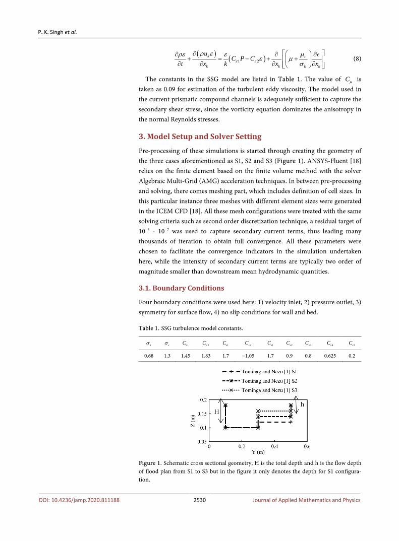
The constants in the SSG model are listed in Table 1. The value of Cµ is taken as 0.09 for estimation of the turbulent eddy viscosity. The model used in the current prismatic compound channels is adequately sufficient to capture the secondary shear stress, since the vorticity equation dominates the anisotropy in the normal Reynolds stresses.

3. Model Setup and Solver Setting

Pre-processing of these simulations is started through creating the geometry of the three cases aforementioned as S1, S2 and S3 (Figure 1). ANSYS-Fluent [18] relies on the finite element based on the finite volume method with the solver Algebraic Multi-Grid (AMG) acceleration techniques. In between pre-processing and solving, there comes meshing part, which includes definition of cell sizes. In this particular instance three meshes with different element sizes were generated in the ICEM CFD [18]. All these mesh configurations were treated with the same solving criteria such as second order discretization technique, a residual target of 10−5 - 10−7 was used to capture secondary current terms, thus leading many thousands of iteration to obtain full convergence. All these parameters were chosen to facilitate the convergence indicators in the simulation undertaken here, while the intensity of secondary current terms are typically two order of magnitude smaller than downstream mean hydrodynamic quantities.

3.1. Boundary Conditions

Four boundary conditions were used here: 1) velocity inlet, 2) pressure outlet, 3) symmetry for surface flow, 4) no slip conditions for wall and bed.

Table 1. SSG turbulence model constants.

kσ εσ 1Cε 2Cε 1sC 2sC 1sC 2sC 3sC 4sC 5sC

0.68 1.3 1.45 1.83 1.7 −1.05 1.7 0.9 0.8 0.625 0.2

Figure 1. Schematic cross sectional geometry, H is the total depth and h is the flow depth of flood plan from S1 to S3 but in the figure it only denotes the depth for S1 configura-tion.

P. K. Singh et al.

DOI: 10.4236/jamp.2020.811188 2531 Journal of Applied Mathematics and Physics

3.2. Inlet (Velocity) and Outlet (Pressure)

At the inlet, turbulence properties i.e. k (turbulence kinetic energy) and (ε tur-bulence dissipation rate) must be specified. These were calculated as [20]:

2k IU= (9) 2

inlett

kCµε ρµ

= (10)

where I is the turbulence intensity, U is the mean value of stream wise velocity and 1000t Iµ µ= .

At the outlet, the pressure condition was given as the boundary condition, and pressure was fixed at zero.

3.3. Wall, Bed and Surface

A no-slip boundary condition was applied at the walls. This means that the ve-locity components should be zero on the walls. Furthermore, the standard wall-function which uses log-law of the wall to compute the wall shear stress was used.

The water surface was defined as a plane of symmetry, which means that the normal velocity and normal gradients of all variables are zero at this plane.

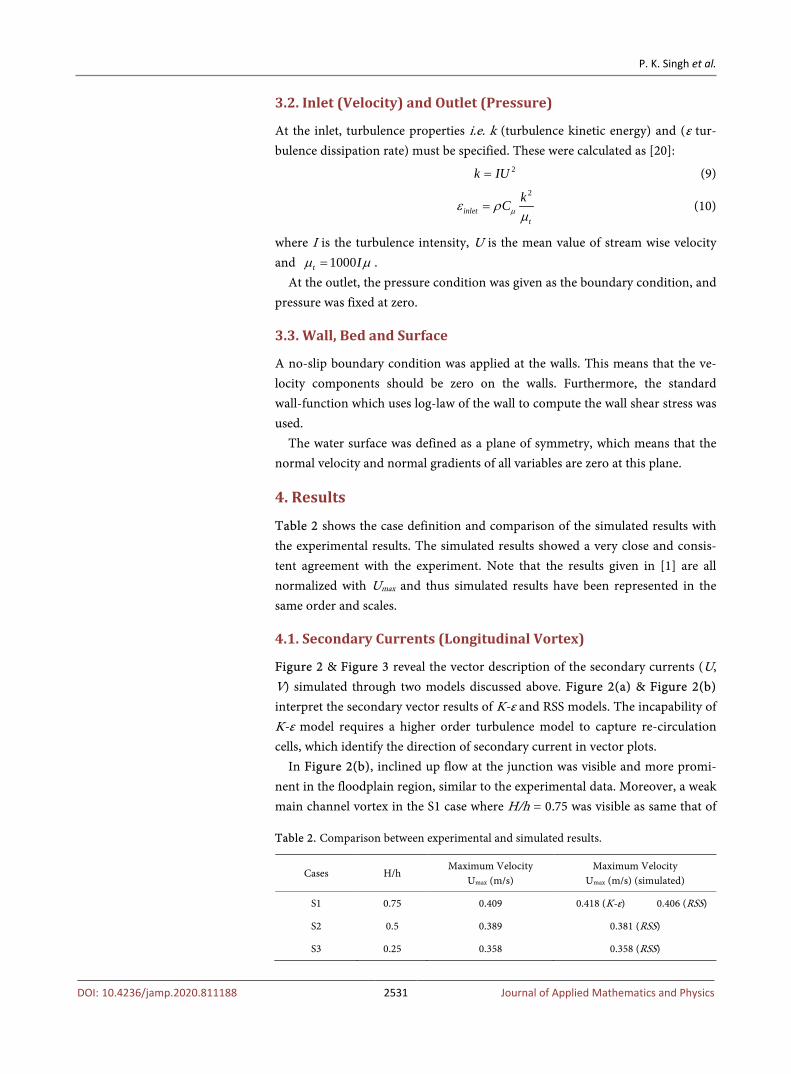
4. Results

Table 2 shows the case definition and comparison of the simulated results with the experimental results. The simulated results showed a very close and consis-tent agreement with the experiment. Note that the results given in [1] are all normalized with Umax and thus simulated results have been represented in the same order and scales.

4.1. Secondary Currents (Longitudinal Vortex)

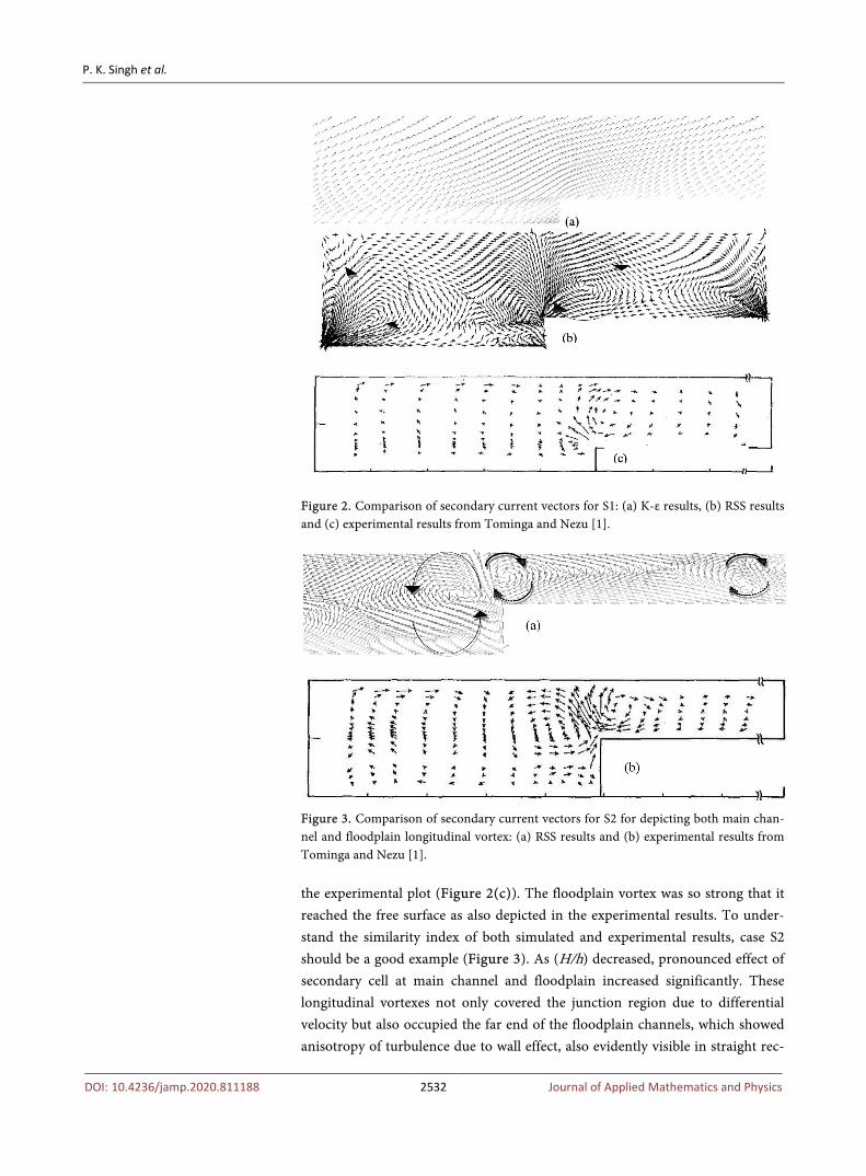
Figure 2 & Figure 3 reveal the vector description of the secondary currents (U, V) simulated through two models discussed above. Figure 2(a) & Figure 2(b) interpret the secondary vector results of K-ε and RSS models. The incapability of K-ε model requires a higher order turbulence model to capture re-circulation cells, which identify the direction of secondary current in vector plots.

In Figure 2(b), inclined up flow at the junction was visible and more promi-nent in the floodplain region, similar to the experimental data. Moreover, a weak main channel vortex in the S1 case where H/h = 0.75 was visible as same that of

Table 2. Comparison between experimental and simulated results.

Cases H/h Maximum Velocity

Umax (m/s) Maximum Velocity

Umax (m/s) (simulated)

S1 0.75 0.409 0.418 (K-ε) 0.406 (RSS)

S2 0.5 0.389 0.381 (RSS)

S3 0.25 0.358 0.358 (RSS)

P. K. Singh et al.

DOI: 10.4236/jamp.2020.811188 2532 Journal of Applied Mathematics and Physics

Figure 2. Comparison of secondary current vectors for S1: (a) K-ε results, (b) RSS results and (c) experimental results from Tominga and Nezu [1].

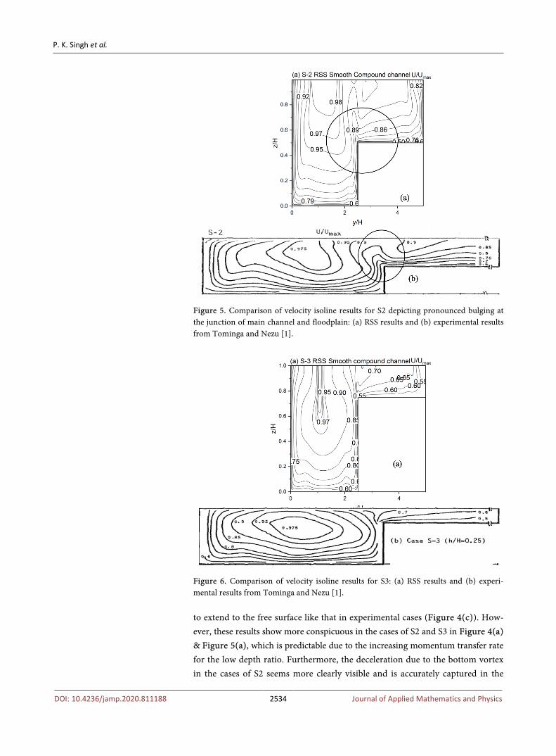
Figure 3. Comparison of secondary current vectors for S2 for depicting both main chan-nel and floodplain longitudinal vortex: (a) RSS results and (b) experimental results from Tominga and Nezu [1].

the experimental plot (Figure 2(c)). The floodplain vortex was so strong that it reached the free surface as also depicted in the experimental results. To under-stand the similarity index of both simulated and experimental results, case S2 should be a good example (Figure 3). As (H/h) decreased, pronounced effect of secondary cell at main channel and floodplain increased significantly. These longitudinal vortexes not only covered the junction region due to differential velocity but also occupied the far end of the floodplain channels, which showed anisotropy of turbulence due to wall effect, also evidently visible in straight rec-

P. K. Singh et al.

DOI: 10.4236/jamp.2020.811188 2533 Journal of Applied Mathematics and Physics

tangular channels [21]. These secondary cells were easily captured in the simu-lated results, although they were missing in the experimental results due to the inability of the data from the weak spots. The two vortices that reached the free surface and covered the junction edge in Figure 3(a) are called main-channel and floodplain vortex, respectively.

Experimentally, the region of vortex given in [1] was in between 1.6 / 3.0y H≤ ≤ which is the same region speculated in our simulation. These results showed the potential of the RSS over the K-ε model and also depicted that the results prom-ise for further investigation on turbulence characteristics in depth for under-standing the interaction of main channel and floodplain flow on simulation ground.

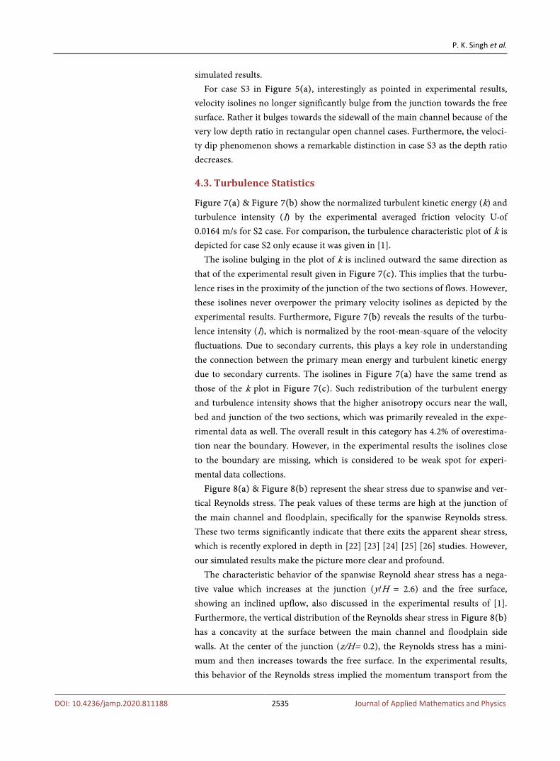
4.2. Distribution of Primary Mean Velocity

For clarity and affirmation on the simulated results for the smooth asymmetric channels, the contour mappings of primary mean velocity are illustrated in Fig-ures 4-6. The experimental results in Figure 4(c), Figure 5(b) & Figure 6(b) show that the isovel line bulges upward in the vicinity of junction edge as a re-sult of the deceleration of velocity, thus pushing towards the bed of the flood-plain and sidewall at the junction. This phenomenon was appropriately mi-micked in the simulated results of the RSS model (Figure 4(b)). This is not sur-prising that the K-ε model in Figure 4(a) was not able to produce the bulging because the high momentum transport at the junction is secondary current in-duced, as not shown before.

In Figure 4(b), in spite of large flow depth at the floodplain, the primary mean velocity isolines are shown with the bulge upward at the junction, while the deceleration due to the low momentum transport from junction edge seems

Figure 4. Comparison of velocity isoline results for S1: (a) K-ε results, (b) RSS results, and (c) experimental results obtained from Tominga and Nezu [1].

P. K. Singh et al.

DOI: 10.4236/jamp.2020.811188 2534 Journal of Applied Mathematics and Physics

Figure 5. Comparison of velocity isoline results for S2 depicting pronounced bulging at the junction of main channel and floodplain: (a) RSS results and (b) experimental results from Tominga and Nezu [1].

Figure 6. Comparison of velocity isoline results for S3: (a) RSS results and (b) experi-mental results from Tominga and Nezu [1].

to extend to the free surface like that in experimental cases (Figure 4(c)). How-ever, these results show more conspicuous in the cases of S2 and S3 in Figure 4(a) & Figure 5(a), which is predictable due to the increasing momentum transfer rate for the low depth ratio. Furthermore, the deceleration due to the bottom vortex in the cases of S2 seems more clearly visible and is accurately captured in the

P. K. Singh et al.

DOI: 10.4236/jamp.2020.811188 2535 Journal of Applied Mathematics and Physics

simulated results. For case S3 in Figure 5(a), interestingly as pointed in experimental results,

velocity isolines no longer significantly bulge from the junction towards the free surface. Rather it bulges towards the sidewall of the main channel because of the very low depth ratio in rectangular open channel cases. Furthermore, the veloci-ty dip phenomenon shows a remarkable distinction in case S3 as the depth ratio decreases.

4.3. Turbulence Statistics

Figure 7(a) & Figure 7(b) show the normalized turbulent kinetic energy (k) and turbulence intensity (I) by the experimental averaged friction velocity U*of 0.0164 m/s for S2 case. For comparison, the turbulence characteristic plot of k is depicted for case S2 only ecause it was given in [1].

The isoline bulging in the plot of k is inclined outward the same direction as that of the experimental result given in Figure 7(c). This implies that the turbu-lence rises in the proximity of the junction of the two sections of flows. However, these isolines never overpower the primary velocity isolines as depicted by the experimental results. Furthermore, Figure 7(b) reveals the results of the turbu-lence intensity (I), which is normalized by the root-mean-square of the velocity fluctuations. Due to secondary currents, this plays a key role in understanding the connection between the primary mean energy and turbulent kinetic energy due to secondary currents. The isolines in Figure 7(a) have the same trend as those of the k plot in Figure 7(c). Such redistribution of the turbulent energy and turbulence intensity shows that the higher anisotropy occurs near the wall, bed and junction of the two sections, which was primarily revealed in the expe-rimental data as well. The overall result in this category has 4.2% of overestima-tion near the boundary. However, in the experimental results the isolines close to the boundary are missing, which is considered to be weak spot for experi-mental data collections.

Figure 8(a) & Figure 8(b) represent the shear stress due to spanwise and ver-tical Reynolds stress. The peak values of these terms are high at the junction of the main channel and floodplain, specifically for the spanwise Reynolds stress. These two terms significantly indicate that there exits the apparent shear stress, which is recently explored in depth in [22] [23] [24] [25] [26] studies. However, our simulated results make the picture more clear and profound.

The characteristic behavior of the spanwise Reynold shear stress has a nega-tive value which increases at the junction (y/H = 2.6) and the free surface, showing an inclined upflow, also discussed in the experimental results of [1]. Furthermore, the vertical distribution of the Reynolds shear stress in Figure 8(b) has a concavity at the surface between the main channel and floodplain side walls. At the center of the junction (z/H= 0.2), the Reynolds stress has a mini-mum and then increases towards the free surface. In the experimental results, this behavior of the Reynolds stress implied the momentum transport from the

P. K. Singh et al.

DOI: 10.4236/jamp.2020.811188 2536 Journal of Applied Mathematics and Physics

Figure 7. Comparison of RSS results for S2 case: (a) turbulent kinetic energy (k), (b) tur-bulent intensity, and (c) experimental results from Tominga and Nezu [1].

Figure 8. (a) Spanwise and (b) vertical Reynolds shear stress terms in case S1, illustrated to be strong at the junction between the sections and near walls.

P. K. Singh et al.

DOI: 10.4236/jamp.2020.811188 2537 Journal of Applied Mathematics and Physics

main channel to floodplain. Thus Figure 8 demonstrates that the momentum transport over the two sections was well captured in this study.

5. Conclusion

The numerical modelling in this study for the smooth asymmetric open channel flows showed consistent results with the experiments. We have discussed the hydrodynamic parameters like secondary current and primary velocity isolines, which showed near exceptional results in capturing major features of flow using the Reynolds shear stress model in CFD. Further analysis of turbulence statistics was given about the interaction of main channel and floodplain flow. The results obtained in this study have shown the capability of the RSS model in capturing the momentum transfer phenomenon at the junction of the edge of the two sec-tions. However, overestimation in the turbulence characteristics has been identi-fied over the bed and wall region. The overall results showed that the internal shear and secondary currents are not negligible and hence should be included in any kind of hydrodynamic studies in compound channels. The distribution of Reynolds shear stress notably indicated the increase in anisotropy at the junction edge, as pointed in the experimental analysis and replicated as well in our simu-lation. In addition, the values near the boundaries were noteworthy in the simu-lated results, which were not visible in the experimental analysis, since these points close to borders are identified and generally overlooked as weak spots.

Acknowledgements

The authors would like to acknowledge the financial support by the National Natural Science Foundation of China (11772270) and the Key Special Fund (KSF-E-17). Furthermore, the authors would also like to thank Akihiro Tomi-naga and Iehisa Nezu for providing in-depth knowledge of compound channel flows via the detailed measurement in their paper.

Conflicts of Interest

The authors declare no conflicts of interest regarding the publication of this paper.

References [1] Tominaga, A. and Nezu, I. (1991) Turbulent Structure in Compound Open-Channel

Flows. Journal of Hydraulic Engineering, 117, 21-41. https://doi.org/10.1061/(ASCE)0733-9429(1991)117:1(21)

[2] Myers, W.R.C. (1978) Momentum Transfer in a Compound Channel. Journal of Hydraulic Research, 16, 139-150. https://doi.org/10.1080/00221687809499626

[3] Tominaga, A. and Knight, D.W. (2004) Numerical Evaluation of Secondary Flow Effects on Lateral Momentum Transfer in Overbank Flows. In River Flow 2004, Proc., 2nd Int. Conf. on Fluvial Hydraulics, Vol. 1, 353-361. https://doi.org/10.1201/b16998-47

[4] Van Prooijen, B.C., Battjes, J.A. and Uijttewaal, W.S. (2005) Momentum Exchange

P. K. Singh et al.

DOI: 10.4236/jamp.2020.811188 2538 Journal of Applied Mathematics and Physics

in Straight Uniform Compound Channel Flow. Journal of Hydraulic Engineering, 131, 175-183. https://doi.org/10.1061/(ASCE)0733-9429(2005)131:3(175)

[5] Tang, X. and Knight, D.W. (2009) Analytical Models for Velocity Distributions in Open Channel Flows. Journal of Hydraulic Research, 47, 418-428. https://doi.org/10.1080/00221686.2009.9522017

[6] Proust, S., Fernandes, J.N., Leal, J.B., Rivière, N. and Peltier, Y. (2017) Mixing Layer and Coherent Structures in Compound Channel Flows: Effects of Transverse Flow, Velocity Ratio, and Vertical Confinement. Water Resources Research, 53, 3387-3406. https://doi.org/10.1002/2016WR019873

[7] Proust, S. and Nikora, V.I. (2020) Compound Open-Channel Flows: Effects of Transverse Currents on the Flow Structure. Journal of Fluid Mechanics, 885. https://doi.org/10.1017/jfm.2019.973

[8] Leighly, J.B. (1932) Toward a Theory of the Morphologic Significance of Turbulence in the Flow of Water in Streams. University of California Press.

[9] Patankar, S. (2018) Numerical Heat Transfer and Fluid Flow. Taylor & Francis. https://doi.org/10.1201/9781482234213

[10] Ferziger, J.H., Perić, M. and Street, R.L. (2002) Computational Methods for Fluid Dynamics. Springer, Berlin, Vol. 3, 196-200. https://doi.org/10.1007/978-3-642-56026-2

[11] Morvan, H., Pender, G., Wright, N.G. and Ervine, D.A. (2002) Three-Dimensional Hydrodynamics of Meandering Compound Channels. Journal of Hydraulic Engi-neering, 128, 674-682. https://doi.org/10.1061/(ASCE)0733-9429(2002)128:7(674)

[12] Morvan, H.P. (2005) Channel Shape and Turbulence Issues in Flood Flow Hydrau-lics. Journal of Hydraulic Engineering, 131, 862-865. https://doi.org/10.1061/(ASCE)0733-9429(2005)131:10(862)

[13] Singh, P.K., Banerjee, S., Naik, B., Kumar, A. and Khatua, K.K. (2018) Lateral Dis-tribution of Depth Average Velocity & Boundary Shear Stress in a Gravel Bed Open Channel Flow. ISH Journal of Hydraulic Engineering, 1-15. https://doi.org/10.1080/09715010.2018.1505562

[14] Singh, P.K., Khatua, K.K. and Banerjee, S. (2018) Flow Resistance in Straight Gravel Bed in Bank Flow with Analytical Solution for Velocity and Boundary Shear Distri-bution. ISH Journal of Hydraulic Engineering, 1-14. https://doi.org/10.1080/09715010.2018.1505561

[15] Rahimi, H.R., Tang, X. and Singh, P. (2020) Experimental and Numerical Study on Impact of Double Layer Vegetation in Open Channel Flows. Journal of Hydrologic Engineering, 25, 04019064. https://doi.org/10.1061/(ASCE)HE.1943-5584.0001865

[16] De Cacqueray, N., Hargreaves, D.M. and Morvan, H.P. (2009) A Computational Study of Shear Stress in Smooth Rectangular Channels. Journal of Hydraulic Re-search, 47, 50-57. https://doi.org/10.3826/jhr.2009.3271

[17] Knight, D.W., Wright, N.G. and Morvan, H.P. (2005) Guidelines for Applying Commercial CFD Software to Open Channel Flow. Report Based on Research Work Conducted under EPSRC Grants GR, 43716, 31.

[18] ANSYS (2018) ANSYS Fluent User’s Guide, Release 19.0. ANSYS, Canonsburg, PA.

[19] Speziale, C.G., Sarkar, S. and Gatski, T.B. (1991) Modelling the Pressure-Strain Correlation of Turbulence: An Invariant Dynamical Systems Approach. Journal of Fluid Mechanics, 227, 245-272. https://doi.org/10.1017/S0022112091000101

[20] Filonovich, M.S., Azevedo, R., Rojas-Solórzano, L.R. and Leal, J.B. (2013) Credibility Analysis of Computational Fluid Dynamic Simulations for Compound Channel

P. K. Singh et al.

DOI: 10.4236/jamp.2020.811188 2539 Journal of Applied Mathematics and Physics

Flow. Journal of Hydroinformatics, 15, 926-938. https://doi.org/10.2166/hydro.2013.187

[21] Nezu, I., Nakagawa, H. and Rodi, W. (1989) Significant Difference between Second-ary Currents in Closed Channels and Narrow Open Channels. The 23rd IAHR Congress, Ottawa, Canada, 125-132.

[22] Singh, P., Tang, X. and Rahimi, H.R. (2019) Apparent Shear Stress and Its Coeffi-cient in Asymmetric Compound Channels Using Gene Expression and Neural Network. Journal of Hydrologic Engineering, 24, 04019051. https://doi.org/10.1061/(ASCE)HE.1943-5584.0001857

[23] Singh, P.K. and Tang, X. (2020) Estimation of Apparent Shear Stress of Asymmetric Compound Channels Using Neuro-Fuzzy Inference System. Journal of Hy-dro-Environment Research, 29, 96-108. https://doi.org/10.1016/j.jher.2020.01.007

[24] Tang, X. (2019) Lateral Shear Layer and Its Velocity Distribution of Flow in Rec-tangular Open Channels. Journal of Applied Mathematics and Physics, 7, 829-840. https://doi.org/10.4236/jamp.2019.74056

[25] Tang, X. and Knight, D.W. (2008) A General Model of Lateral Depth-Averaged Ve-locity Distributions for Open Channel Flows. Advances in Water Resources, 31, 846-857. https://doi.org/10.1016/j.advwatres.2008.02.002

[26] Singh, P. and Tang, X. (2020) Zonal and Overall Discharge Prediction Using Mo-mentum Exchange in Smooth and Rough Asymmetric Compound Channel Flows. Journal of Irrigation and Drainage Engineering, 146, 05020003. https://doi.org/10.1061/(ASCE)IR.1943-4774.0001493