On the Use of Formative Measurement Specifications in Structural Equation Modeling: A Monte Carlo...
43
Christian M. Ringle, Oliver Götz, Martin Wetzels, Bradley Wilson On the Use of Formative Measurement Specifications in Structural Equation Modeling: A Monte Carlo Simulation Study to Compare Covariance-Based and Partial Least Squares Model Estimation Methodologies RM/09/014
-
Upload
tu-harburg -
Category
Documents
-
view
1 -
download
0
Transcript of On the Use of Formative Measurement Specifications in Structural Equation Modeling: A Monte Carlo...

Christian M. Ringle, Oliver Götz, Martin Wetzels, Bradley Wilson On the Use of Formative Measurement Specifications in Structural Equation Modeling: A Monte Carlo Simulation Study to Compare Covariance-Based and Partial Least Squares Model Estimation Methodologies RM/09/014

On the Use of Formative Measurement Specifications in Structural
Equation Modeling: A Monte Carlo Simulation Study to Compare
Covariance-Based and Partial Least Squares Model Estimation
Methodologies
Christian M. Ringle; University of Hamburg; Faculty of Business, Economics and Social
Sciences; Von-Melle-Park 5; 20146 Hamburg; Germany; e-mail: [email protected]
hamburg.de
Oliver Götz; University of Münster; Marketing Centrum Münster;
Am Stadtgraben 13-15; 48143 Münster; Germany; e-mail: [email protected]
Martin Wetzels; Maastricht University; Faculty of Economics and Business Administration;
P.O. Box 616; 6200 MD Maastricht; The Netherlands; e-mail: [email protected]
Bradley Wilson; RMIT University; School of Applied Communication;
GPO Box 2476V; Melbourne VIC 3001; Australia; e-mail: [email protected]

1
On the Use of Formative Measurement Specifications in Structural
Equation Modeling: A Monte Carlo Simulation Study to Compare
Covariance-Based and Partial Least Squares Model Estimation
Methodologies
Abstract
The broader goal of this paper is to provide social researchers with some analytical guidelines
when investigating structural equation models (SEM) with predominantly a formative
specification. This research is the first to investigate the robustness and precision of
parameter estimates of a formative SEM specification. Two distinctive scenarios (normal and
non-normal data scenarios) are compared with the aid of a Monte Carlo simulation study for
various covariance-based structural equation modeling (CBSEM) estimators and various
partial least squares path modeling (PLS-PM) weighting schemes. Thus, this research is also
one of the first to compare CBSEM and PLS-PM within the same simulation study. We
establish that the maximum likelihood (ML) covariance-based discrepancy function provides
accurate and robust parameter estimates for the formative SEM model under investigation
when the methodological assumptions are met (e.g., adequate sample size, distributional
assumptions, etc.). Under these conditions, ML-CBSEM outperforms PLS-PM. We also
demonstrate that the accuracy and robustness of CBSEM decreases considerably when
methodological requirements are violated, whereas PLS-PM results remain comparatively
robust, e.g. irrespective of the data distribution. These findings are important for researchers
and practitioners when having to choose between CBSEM and PLS-PM methodologies to
estimate formative SEM in their particular research situation.

2
Introduction
Structural Equation Modeling (SEM) with latent variables is becoming increasingly popular
in social and behavioral science (Boomsma, 2000) . The literature on SEM distinguishes
between two different operationalizations of the relationships between latent variables and
their observed indicators: the reflective (principal factor) and the formative (composite index)
measurement models of latent variable. Numerous studies have by default or erroneously by
design incorrectly specified their items as reflective when they should have used a formative
measurement model operationalization (Jarvis, MacKenzie, & Podsakoff, 2003). This is
somewhat surprising considering the fact that the understanding of formative indicator
orientation is not new (Blalock, 1971) and previous research has focused on the nature,
identification, and validation issues of formative indicators (Bollen & Lennox, 1991;
Diamantopoulos & Winklhofer, 2001; Edwards & Bagozzi, 2000; MacCallum & Browne,
1993).
There are two statistical methodologies for estimating SEM with latent variables
incorporating formative measurement models: the covariance-based (CBSEM) and the partial
least squares path modeling (PLS-PM). A common misunderstanding found in the literature
is that only PLS-PM allows the estimation of SEM that includes formative measurement
models. Even though it has often been neglected, CBSEM is also capable of handling
formative specifications, but requires that the model’s identification be guaranteed and, thus,
that certain model specification rules are followed. These CBSEM specification issues have
been thoroughly addressed by MacCallum & Browne (1993).
Despite the broad discussion and establishment of the formative measurement model
operationalization as a reasonable alternative to the reflective SEM mode, little attention has

3
so far been devoted to the conditions under which formative measures and their estimation
method lead to precise and robust coefficients for the population sample (Browne, 1984).
Some CBSEM estimators require the observed variables to be multivariate normally
distributed. Violation of this assumption may distort the standard error of the path coefficient
and parameters of the measurement models. However, the majority of data collected in
behavioral research do not follow multivariate normal distributions (Micceri, 1989). This
property is exacerbated with the use of formative indicators. It would be unreasonable to
expect the observed data to follow a multivariate normal distribution in the population when
using formative indicators.
Consequently, it is important to fully understand the effects of non-normality with respect to
the accuracy and robustness of formative indicators in SEM. Our research is positioned to fill
this gap in the literature, and this paper aims to contribute to the body of knowledge on the
structural equation model specifications with formative (cause) indicators. The uniqueness of
this study is twofold. It is the first one to investigate a model that primarily consists of
formative measurement models by conducting a Monte Carlo simulation study to investigate
the use of formative measurement model operationalization. Secondly, it is also the first one
to compare the robustness and performance of CBSEM with respect to different estimator
discrepancy functions, in concert with PLS-PM and its’ different path weighting schemes. In
this paper, we are mindful of the advice of Boomsma & Hoogland (2001) who, referring to a
CBSEM context, stated that:
The key objective of robustness research is to offer practical guidelines for applied work, so as to prevent non-robust analyses that would inevitably lead to wrong substantive inferences. Within that framework, a predominant question is: if structural models are to be analyzed, what estimation methods have to be preferred under what conditions? (p. 22)

4
Therefore, the objectives of this research are: (a) to demonstrate the implications of formative
measurement model use in SEM, (b) to systematically and empirically test the accuracy and
robustness of SEM methods with formative measurement models by using Monte Carlo
simulations, and (c) to provide recommendations regarding the appropriate selection of SEM
methods, given their specific research requirements.
This paper is organized as follows: We outline issues relevant to the operationalizing of
formative measurement models and then address the methodological aspects of CBSEM and
PLS-PM with regard to estimating formative relationships within SEM. Building on the
findings of a literature review, we explain the design of our primary Monte Carlo simulation
study on estimating a SEM that predominantly involves formative measurement model
operationalizations by the means of the CBSEM and PLS-PM methodologies. Then, we
highlight the pertinent results for each method and present a comparison of these analytical
outcomes. Finally, we discuss the substantive implications of our findings for SEM
applications and suggest future avenues for further research.
Formative Measurement Model Operationalization
Structural equation modeling applications often involve latent constructs with multiple
indicators. The measurement or outer model specifies the relationship between observable
variables (i.e., indicators) and latent variables. The direction of relationships and their
causality is either in an effect (reflective) or a cause (formative) mode (Bollen, 1989;
MacCallum & Browne, 1993). When discussing the nature and direction of relationships
between constructs and observed measures, the literature on construct validity and associated
measurement issues primarily emphasizes the reflective mode. The reflective measurement
model has its roots in traditional test theory and psychometrics (Nunnally & Bernstein, 1994).

5
Each indicator represents an error-afflicted measurement of the latent variable. The direction
of causality is from the construct to the indicators and observed measures are assumed to
reflect variation in latent constructs. Altering the construct is therefore expected to manifest
in changes in all the multi-item scale indicators.
Research on SEM recognizes that in the early stages of model development and in some
situations, it is appropriate to determine causality from the measures to the construct, rather
than vice versa (Blalock, 1971). Therefore, formative constructs have to be modeled as a
(usually linear) combination of their indicators plus a disturbance term (Diamantopoulos,
2006). A frequently cited example of formative measurement is socio-economic status (SES),
which is viewed as a composite of social and economic indicators such as occupation,
education, residence, and income. If any one of these measures decreases, SES would
decline. Figure 1 clarifies this issue: the arrows either point from the construct to the
(reflective mode) indicators, or in the opposite direction.
-----------------------------------
Insert Figure 1 about here
-----------------------------------
Some researchers provide a conceptual discussion of the differences between formative and
reflective measurement models (Bollen & Lennox, 1991; Diamantopoulos & Winklhofer,
2001; Edwards & Bagozzi, 2000) and design rules for determining the specific type of
measurement model (Jarvis, MacKenzie, & Podsakoff, 2003). Based on these studies, the
decision to use formative measurement models in SEM has specific implications for
researchers.

6
One implication of the direction of causality is that omitting one indicator could omit a
unique part of the formative measurement model and change the meaning of the variable
(Diamantopoulos & Winklhofer, 2001). Thus, some researchers maintain that a formative
measurement model requires a census of all indicators that determine the construct (Jarvis,
MacKenzie, & Podsakoff, 2003). It is therefore quite obvious that formative indicators
frequently do not follow a multinormal distribution. The response profile of our previous
example leads to non-normal item distribution curves with varying degrees of skewness and
kurtosis. This violation of multivariate normality can invalidate statistical hypothesis testing
and strongly influence the choice of SEM estimations (Browne, 1984). It is clear that this
area requires more research attention. Consequently, simulation studies need to investigate
the different CBSEM and PLS-PM statistical estimation techniques to compare their relative
performance in situations involving non-normal formative indicators. This type of research
will lead to a better understanding of each method’s robustness and precision in this specific
research situation.
Formative Structural Equation Modeling Techniques
Two main approaches have been used to estimate formative measurement models within
structural models: the CBSEM and the PLS-PM methods. Both methods have distinctive
statistical characteristics (Fornell & Bookstein, 1982; Schneeweiß, 1991) and selecting an
approach to SEM depends on the particular research situation. CBSEM is the method of
choice for theory testing, while PLS-PM is appropriate for prognosis-oriented applications
(Wold 1982b).
In CBSEM (see Rigdon, 1998), the parameter estimation of a given model minimizes the
difference between the implied covariance matrix and the sample covariance matrix, with the

7
final result permitting the appropriate model fit to be determined. There are alternative
CBSEM estimation techniques available to the researcher. The most commonly used
approaches include: maximum likelihood (ML), generalized least squares (GLS), unweighted
least squares (ULS), and asymptotic distribution free (ADF) estimation (Marcoulides &
Hershberger, 1997). These CBSEM methods vary in their particular minimization of the
discrepancy function, thereby including specific assumptions, for example, regarding sample
size or the multivariate
(non-) normality of data.
The inclusion of formative measures in CBSEM has been well documented by Jöreskog &
Sörbom (2001) and Jöreskog & Goldberger (1975). Williams, Edwards, & Vandenberg
(2003) point out that formative indicators could be modeled in CBSEM by respecifying the
formative indicators as latent exogenous variables with single indicators, fixed unit loadings,
and a fixed measurement error. MacCallum & Brown (1993) illustrate various other
formative model specifications that have adequate model identification. Consequently, if the
hypothesized structural and measurement model is correct in the sense that it explains the
covariance of all the indicators under the given assumption of different estimation methods, it
is believed that the covariance-based methods should provide optimal estimates of the model
parameters.
Instead of using the model to explain the covariance of all the indicators, the PLS-PM
methodology (Wold, 1973, 1974, 1982a, 1982b) maximizes the variance of all dependent
variables. Thus, parameter estimates are obtained based on the ability to minimize the
residual variances of dependent (latent and observed) variables. To obtain the weights and
subsequent loadings and structural estimates, the PLS-PM approach uses a two-stage

8
estimation algorithm (Lohmöller, 1989). In the first stage, after an initial, rather arbitrary,
estimation of the latent variables, the process iteratively switches between the measurement
and the structural model approximation by means of simple and/or multiple regressions until
the parameter estimates converge into a set of weights used for estimating the latent variable
scores. The PLS algorithm thereby aims at minimizing the residual variance of latent
endogenous variables. The second stage involves a non-iterative application of ordinary least
squares regression to obtain the loadings, weights, structural estimates, mean scores, and
location parameters of the latent and observed variables. Three different kinds of weighting
schemes have been used in this context: centroid, factor, and path weighting. Lohmöller
(1989) and Tenenhaus, Vinzi, Chatelin, & Lauro (2005), for instance, present a general
descriptions of the PLS methodology, particularly of the estimation of formative
measurement models, whilst Chin (1998) presents a catalog of non-parametric model PLS-
PM evaluation criteria as this statistical approach does not offer global goodness of fit criteria
as CBSEM does.
In respect of a comparison of CBSEM and PLS (see Lohmöller, 1989), McDonald (1996)
points out that Wold’s (1980) (reflective) PLS Mode-A algorithm, like the ULS Method in
CBSEM, maximizes the sum of the covariances of directly connected composites (subject to
normalized weights). It furthermore allocates a (generally under-identified) rank one
approximation to the individual correlations across the connected blocks of latent variables
and their respective measurement models. On the other hand, Wold’s (1980) (formative) PLS
Mode-B algorithm maximizes the sum of correlations between connected blocks. It has no
exact counterpart in CBSEM and McDonald (1996) conjectures that it would be difficult to
empirically find or construct cases in which the results of PLS Mode-B and certain CBSEM
methods (other than ULS) differ notably. Hence, we designed a simulation study and

9
conducted computational experiments to provide both researchers and practitioners with
additional confidence regarding their decision to select an appropriate estimation technique
for SEM incorporating formative measurement models.
Literature Review
A substantial number of simulation studies on CBSEM (e.g. Boomsma, 1983; Boomsma &
Hoogland, 2001; Paxton, Curran, Bollen, Kirby, & Chen, 2001; Satorra, 1990; Stephenson &
Holbert, 2003) primarily compare alternative CBSEM discrepancy functions and investigate
their estimation bias, accuracy, and robustness with respect to sample size, and third and
fourth-order data moments. Paxton, Curran, Bollen, Kirby, & Chen (2001), for example,
provide an introduction to the design and implementation of a Monte Carlo simulation within
the SEM area. These authors also present a comparison of the maximum likelihood and two-
stage least squares with regard to different sample sizes and misspecifications. Boomsma &
Hoogland (2001) conclude that there are non-convergence problems and improper CBSEM
solutions in small samples (200 and less). Furthermore, under various non-normal conditions,
maximum likelihood estimators in respect of large models have relatively good statistical
properties compared to other CBSEM estimators. Satorra (1990) indicates that generally
maximum likelihood and weighted least squares are robust against the violation of
distributional assumptions. We do not intend to review the whole plethora of CBSEM
robustness studies (especially those with reflective specifications) as this knowledge is
assumed of the reader. Instead, focus is given to the discussion of previous study results
centered on formative model specifications. Even a cursory review will reveal that the
majority of analyses have been presented with models dominant in reflective specifications.

10
With respect to PLS-PM, it is difficult to find published robustness studies compared with the
vast work already completed in the CBSEM realm. There are only a few publications
utilizing PLS-PM that follow this line of research. Cassel, Hackl, & Westlund (1999) have
performed a robustness simulation study on PLS-PM estimates by concentrating on varying
the skewness of reflective indicators and having multicollinearity between latent variables
and an artificial model misspecification. Their simulation results indicate that PLS-PM based
on reflective measurement models is quite robust against skewness, as well as against
multicollinearity between latent variables and misspecification due to the omission of a latent
variable in the structural model. In respect to inner model coefficients, substantial effects are
only observed on the estimates of extremely skewed data and for the erroneous omission of a
highly relevant exogenous latent variable.
Chin & Newsted (1999) employ a Monte Carlo simulation for their analysis on PLS-PM with
small samples. They find that the PLS approach can provide information about the
appropriateness of indicators at sample size as low as 20. This study confirms the consistency
at large (Jöreskog & Wold, 1982) in that the PLS-PM estimates will be asymptotically correct
under the joint conditions of consistency: large sample size and large number of indicators
per latent variable. Moreover, Chin, Marcolin, & Newsted (2003) employ a PLS-PM Monte
Carlo simulation for an interactions effect model for varied sample sizes, altered numbers of
indicators, and for the loading structure of manifest variables in respect of each of the
constructs in their model. They finally provide a comparison of the SEM that incorporates
latent variables with a summated scales approach. The authors provide evidence that
increasing the number of reflective indicators will have a stronger impact on consistent
estimations than increasing the sample size will have. This also holds for higher loadings and
the associated reliabilities.

11
To date, there are only a handful of studies that compare the parameter estimates of both
CBSEM and PLS-PM methods. Tenenhaus, Vinzi, Chatelin, & Lauro (2005) analyze a
European customer satisfaction index (ECSI) model by means of reflective measures to
compare CBSEM and PLS-PM estimates. They find that the outcomes of both methods are at
comparable levels, but that CBSEM provides higher R2 outcomes for the latent endogenous
variables and that PLS-PM exhibits higher correlations between indicators and their
associated latent variable. The latter is due to the PLS-PM estimation being more data driven
and being more substantially influenced by the manifest variables.
The Hsu, Chen, & Hsieh (2006) article features robustness testing of a reflective
measurement model orientation. They compare various estimators, including a more recent
artificial neural network-based (ANN) SEM technique, PLS-PM, and CBSEM estimations of
200 simulated samples in respect of various scenario designs (e.g., skewness of data). The
simulated model only consists of reflective measures and is based on a simple ECSI model
structure. Hsu, Chen, & Hsieh (2006) find that the ANN-based SEM technique is similar to
PLS-PM and conclude that all SEM techniques offer a certain robustness with respect to
skewness of data. The results from this study confirm that PLS-PM underestimates structural
path coefficients and that CBSEM is more sensitive to small sample size problems that
experience larger deviations.
Our literature review reveals that PLS-PM overestimates the outer loadings of latent
constructs and provides more conservative estimates of the inner model than ML-CBSEM.
Furthermore, compared to symmetrical data, PLS-PM and ML-CBSEM estimates that
incorporate reflective measurement models are negligibly influenced by skewness. CBSEM

12
methods are also more sensitive to small sample sizes than PLS-PM. It can thus be concluded
that research on formative measures is still in its early stages regarding the precision and
robustness of coefficients. The review of the literature supports our premise that there has
been a dearth of robustness studies undertaken specifically comparing CBSEM and PLS-PM
with a formative model specification.
Design of the Simulation Study
As we have previously outlined, a researcher has the choice of utilizing CBSEM and PLS-
PM when investigating formative SEMs. This raises the question of which approach to select
for SEM applications containing formative measurement models of the latent exogenous
variables. A Monte Carlo simulation study (Paxton, Curran, Bollen, Kirby, & Chen, 2001)
allows us to address this critical question. Our Monte Carlo design allows us to
systematically study the bias, accuracy, and robustness for both the CBSEM and PLS-PM
techniques’ parameter estimates. The SEM underpinning our design and subsequent analyses
(Figure 2) consists of three latent exogenous variables (ξ1, ξ2 and ξ3) and two latent
endogenous variables (η1 and η2). The manifest variables in the measurement models of the
latent exogenous variables are formatively operationalized, while the latent endogenous
variables are measured reflectively. This simple design specification has been selected for our
simulation for an unambiguous investigation of the effects of non-normality by means of
different SEM methods.
-----------------------------------
Insert Figure 2 about here
-----------------------------------
Researchers have to ensure that their CBSEM has been identified to indicate that the model
fit is indeed a reasonable presentation of the phenomena under investigation. Approaches to

13
test identification (Rigdon, 1995) include following certain rules but also resolving algebraic
solutions, analyzing the information matrix, and evaluating the augmented Jacobian matrix.
The model presented in Figure 2 has been identified, because there are more equations
describing the model than unknown parameters. However, MacCallum & Browne (1993)
address the issue of model identification in CBSEM when formative measurement models are
involved. In keeping with their rules – especially with respect to the formative latent
exogenous variables ξ1 and ξ3, which have only one relationship to a latent endogenous
variable – the variance values of the latent endogenous variables η1 and η2 need to be set to
one in addition to applying the usual reflective CBSEM parameter constraints (Rigdon,
1998). The model in Figure 2 is also appropriate for PLS-PM. Besides other aspects, the
model is recursive, latent variables are estimated by non-overlapping blocks of manifest
variables, and the model operationalization fits the PLS-PM-specific assumptions of predictor
specification (Chin, 1998; Lohmöller, 1989; Tenenhaus, Esposito Vinzi, Chatelin, & Lauro,
2005).
The underlying correlation matrix (Table 5 in the Appendix) of the data generation procedure
has some unique characteristics that are important to note for this study. The manifest
variables x1, x2, and x3 are slightly to moderately correlated, while x4 and x5 have very low
correlations with other manifest variables in the ξ1 measurement model. However, x4 and x5
are strongly correlated with the indicators of the latent variables η1 and η2, while this does
not hold for x1, x2, and x3. The manifest variables x6, x7, and x8 in the measurement model of
the latent exogenous variable ξ2 are poorly correlated. Here, only x6 and x7 have significant
correlations with the η1 and η2 indicators. The manifest variables x9 to x13 in the ξ3
measurement model are slightly to moderately correlated. All five manifest variables have
significant correlations with the indicators of the latent endogenous variable η2. Finally, the

14
manifest variables y1, y2, and y3 in the measurement model of the latent endogenous η1
exhibit strong correlations. The same pattern holds for the η2 indicators. The information on
the correlation pattern is important for analyzing the simulation results.
-----------------------------------
Insert Table 1 about here
-----------------------------------
In this study, we pre-specify the relationships in the SEM according to Table 1 and then
simulate data for the given parameters. The data generation process is consistent with the
procedure described by Chin, Marcolin, & Newsted (2003) for a Monte Carlo PLS-SEM
study. We developed a STATISTICA 7.1 (StatSoft, 2005) macro implementation to perform
this type of approach in two studies: one on multivariate normal data and one on extremely
non-normal data.
The first Monte Carlo simulation study includes the generation of 1000 sets of multivariate
normal data that meet – in an evaluation of data simulation (Boomsma & Hoogland, 2001) –
the expected raw data characteristics, impart convergence of CBSEM estimations, as well as
proper solutions for the structural model regarding the positive sign of variances. Each data
set consists of 300 cases, which is a large enough number for model estimation, as well as
matching the average sample size of SEM simulation studies presented in academic literature
(Stephenson & Holbert, 2003). Although simulation studies on CBSEM (e.g. Curran, Bollen,
Paxton, Kirby, & Chen, 2002; Hu & Bentler, 1999; Marcoulides & Saunders, 2006; Satorra
& Bentler, 2001) and PLS-PM (e.g. Cassel, Hackl, & Westlund, 1999; Chin, Marcolin, &
Newsted, 2003) present varying sample sizes to answer specific methodological research
questions, we do not add this level of complexity, which would also require systematic
alteration of the number of indicators in the measurement models. In this study, we

15
concentrate on CBSEM and PLS-PM comparisons for formative indicator specification.
Previous simulation studies on reflective CBSEM indicate that 300 cases are sufficient to
provide robust estimations, at least for ML-CBSEM estimation (Boomsma & Hoogland,
2001).
The second Monte Carlo simulation study undertaken in this investigation includes the same
analytical design for non-normal data. The non-normal data specification has a skewness of
two and kurtosis of eight, whereby the generation of non-normal multivariate random
parameter values follows the Vale & Maurelli (1983) procedure implemented in the
STATISTICA 7.1 program. This method is an extension of Fleishman’s (1978) approach and,
in comparison to other methods, fits our non-normal data generation purposes better
(Reinartz, Echambadi, & Chin, 2002). The Vale & Maurelli (1983) technique can be used to
generate adequate multivariate random numbers with pre-specified intercorrelations and
univariate means, variances, skews, and kurtosis as efficiently as possible.
Both approaches, CBSEM and PLS-PM, are applied on the SEM in Figure 2 and on each set
of data in the normal, as well as in the non-normal data scenario. This is undertaken
contrasting CBSEM standard estimators (ML, GLS, ADF and ULS) and PLS-PM weighting
schemes (centroid, factor, and path). The CBSEM computational results are also obtained via
STATISTICA 7.1 software by employing a macro program that the authors designed for this
study. In addition, a batch computing module was developed to process the simulated data by
means of the SmartPLS 2.0 (Ringle, Wende, & Will, 2005) software to obtain PLS-PM
results.

16
Results of the Monte Carlo Simulation Study
The Monte Carlo simulation presented in this study generates normal and non-normal data
for a SEM incorporating formative operationalization of latent exogenous variables. These
data are used to compare the model parameter estimations of the four main CBSEM
discrepancy function procedures. Furthermore, our simulation study evaluates PLS-PM
estimations that employ the different centroid, factor, and path inner model weighting
schemes (Tenenhaus, Esposito Vinzi, Chatelin, & Lauro, 2005). Finally, we compare the
CBSEM and PLS-PM results of the normal and non-normal data scenarios.
Comparison of Alternative CBSEM Model Estimation Techniques
In CBSEM, the parameters of a proposed model are estimated by minimizing the discrepancy
between the empirical covariance matrix and a covariance matrix implied by the model. The
common methods to measure this discrepancy are ML, GLS and ULS. The ADF/WLS
method is a generalization of the other three CBSEM discrepancy functions that use a weight
matrix based on a direct estimation of the residuals’ fourth-order moments (Satorra &
Bentler, 2001). When comparing the average formative model CBSEM estimates of the 1000
sets of normal and non-normal data, we find that the ML (Tables 2 and 3), GLS, and the
ADF/WLS procedure exhibit roughly the same results pattern (Tables 6 to 9 in the
Appendix).
ML and GLS perform at almost comparable levels. The only exception is the robustness of
the formative measurement model estimates in the non-normal data scenario, with ML
providing significantly better outcomes. ADF/WLS performs considerably weaker than the
other two methods do. This study’s results of the formative CBSEM model estimator
performance are consistent with Boomsma & Hoogland’s (2001) findings with regard to
17
reflective measurement models and the same selected number of cases. Our results are
therefore in line with our expectations regarding the methodological characteristics of the
discrepancy functions. The GLS and especially the ADF/WLS model estimation techniques
usually require a high number of observations (several thousand) to provide robust outcomes.
Consequently, the GLS and ADF/WLS results of small and medium-sized samples should
also be interpreted with caution in formative SEM.
The ADF/WLS or ULS for model estimation relaxes the hard assumptions regarding the
multivariate normality of the data when utilizing the ML or GLS estimator. ULS is a special
ADF/WLS case and these methods do not automatically reveal standard errors or an overall
chi-square fit statistic, but provide consistent estimates that are comparable to ML and seem
relatively robust (Satorra, 1990). However, in our analysis, ULS does not fit the results
pattern of the other CBSEM techniques. The average parameter estimations differ strongly
from the given relationships and exhibit elevated deviations and relatively high outliers.
McDonald (1996) confirms that ULS is equivalent to the reflective PLS-PM model
estimation and is thus, ideally, not suited for our study of formative SEM measurement model
operationalization. Consequently, it appears that in respect of the simulated scenarios that we
investigated, ML provides the most appropriate CBSEM estimates, especially with regard to
the moderate study sample size and specified formative model.
Comparison of Alternative PLS Model Estimation Techniques
The next analysis compares the outcomes of the centroid, factor, and path inner model PLS
weighting schemes (Chin, 1998; Lohmöller, 1989; Tenenhaus, Esposito Vinzi, Chatelin, &
Lauro, 2005). Applications of PLS illustrate that the alternative inner model weighting
schemes only lead to marginal differences in the PLS-PM model estimates. Our simulation

18
study confirms this observation (Lohmöller, 1989; Tenenhaus, Esposito Vinzi, Chatelin, &
Lauro, 2005). On average, the alternative weighting schemes provide the same parameter
estimates for the model under investigation (Table 10 in the Appendix).
Comparison of CBSEM and PLS-PM
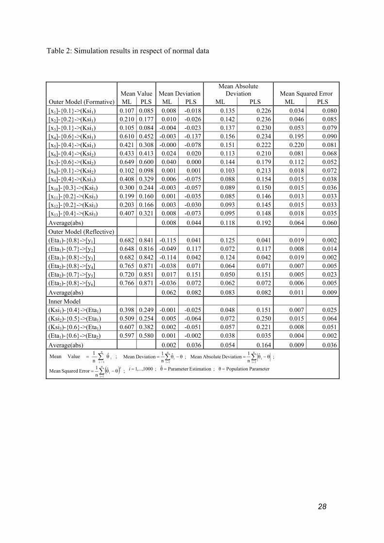
In our last analysis, we compare CBSEM and PLS-PM estimates for normal (Table 2) and
non-normal (Table 3) data scenarios. This comparison for the cause-effect model employs
ML, which offers the most suitable CBSEM parameter estimations in this simulation study.
Our previous results illustrate that alternative PLS-PM inner weighting schemes provide
almost identical results; we therefore only present PLS results for the path-weighting scheme
as it is most frequently used in PLS-PM applications (Chin, 1998). In our computational
experiments for normal and non-normal data constellations, the comparison of CBSEM and
PLS-PM parameter estimates includes their bias (mean deviation), accuracy (mean absolute
deviation), and robustness (mean squared error).
-----------------------------------
Insert Table 2 about here
-----------------------------------
Mean Deviation. Based on the mean deviation, the simulation study reveals that the ML-
CBSEM estimation has a tendency to overestimate the true parameter values, while the PLS-
PM has the reverse tendency, i.e. underestimating parameters in formative measurement
models (for both normal and non-normal scenarios). It is notable that a bias in the opposite
direction holds in respect of reflective outer measurement models, whereas ML-CBSEM has
a tendency to underestimate and PLS-PM to overestimate the true values (for both
simulations). Finally, ML-CBSEM tends to overestimate the inner relationships in the normal
data scenario and exhibits both directions – overestimation and underestimation of

19
parameters – in the non-normal data scenario, while PLS-PM completely underestimates
those parameters in both simulation scenarios.
-----------------------------------
Insert Table 3 about here
-----------------------------------
Mean Absolute Deviation. In the formative outer model, ML-CBSEM outperforms PLS-PM
in all parameter estimations regarding accuracy in terms of the mean absolute deviation
(MAD). It is important to note that both methods perform considerably better in the formative
measurement model of latent exogenous variable ξ3 compared to ξ1 and ξ2. The formative
indicators of the latter two latent variables consist of a heterogeneous correlation pattern,
while those of the manifest variables in the ξ3 measurement model are relatively
homogenous. In the inner model, ML-CBSEM and PLS-PM perform with great precision
regarding the relationship between the latent endogenous variables η1 and η2. The MAD for
the relationships between the latent exogenous ξ1, ξ2 and ξ3 variables and the latent η1
endogenous variable has a weaker outcome– especially in the case of PLS-PM, which is
considerably less accurate in these relationships than ML-CBSEM – although this outcome is
still at a relatively high level. The highest estimation precision is found in the reflective
measurement models where the MAD for both methods is at a comparable level. Both
procedures reveal two indicators with a significantly higher MAD: With regard to ML-
CBSEM, both of these relationships are in the outer model of η1 (paths to y1 and y3), while
PLS-PM has one indicator with a higher MAD in each of the reflective measurement models
(paths from η1 to y2 and η2 to y4). The accuracy of ML-CBSEM estimates decrease
significantly with regard to the non-normal data scenario in all model relationships, whereas
PLS-PM performs very well and only experiences a slight decrease in deviation with regard
to the formative outer models (Table 4).

20
-----------------------------------
Insert Table 4 about here
-----------------------------------
Mean Squared Error. The mean squared error (MSE) provides additional information about
the robustness of ML-CBSEM and PLS-PM parameter estimates. In the formative
measurement model and in accordance with the MAD, we find that in the normal data
example both methods have the lowest MSE of the parameter estimates for the latent variable
ξ3, which has indicators with a homogenous correlation pattern. Here, the difference between
the maximum and minimum MSE is 0.005 for ML-CBSEM and 0.005 for PLS-PM, revealing
the high robustness of the computations within the measurement model. In contrast, the MSE
is substantially higher in the outer relationships of the latent variables ξ1 and ξ2. It is
important to note that ML-CBSEM produces many estimates that deviate strongly from the
true constrained population parameters, resulting in an increased MSE. This is most apparent
with those manifest variables that have a high correlation pattern with the indicators of the
latent endogenous variables and, consequently, a high pre-specified outer relationship. The
difference between the maximum and minimum MSE is 0.186 in respect of the outer
relationships of ξ1 and 0.063 for ξ2, indicating a reduced robustness of the ML-CBSEM
parameter estimates. We did not find any comparable patterns in respect of the MSE of the
measurement models estimated with PLS-PM in the normal data scenario. Here, the
difference between the maximum and minimum MSE is 0.011 for the outer relationships of
ξ1 and 0.020 for ξ2, representing a loss of robustness within the measurement model in
comparison to ξ3, but a much better result compared to the ML-CBSEM estimation.

21
We find that ML-CBSEM tends to generate more erratic results– which are associated with
high estimation errors (the difference between the estimated and expected path coefficients) –
in respect of some indicators, while computations for others in the same, critical latent
variable measurement model are robust. On the other hand, PLS-PM exhibits an equal and
slight level of volatility regarding estimation errors in respect of all indicators and,
consequently, a higher robustness for the estimated ξ1 and ξ2 outer relationships. In contrast,
the MSE is considerably lower in the reflective outer models and principally performs at
comparable levels in respect of ML-CBSEM and PLS-PM. Finally, the simulation study’s
inner model estimates provide MSE findings that are similar to those described in respect of
the MAD.
A comparison of the normal data with the non-normal data scenario of these analytical results
provides evidence that ML-CBSEM estimates increase their MSE considerably and, thus,
decrease their robustness in all model relationships (Table 4). In contrast, PLS-PM only
exhibits a slight MSE increase in respect of the formative measurement models, whereas the
robustness of the parameter estimation does not substantially change in respect of the outer
reflective and inner model relationships.
Summary and Conclusion
Researchers in the social sciences disciplines are swiftly moving towards using formative
constructs within their SEM analyses. CBSEM and PLS-PM are two distinctive statistical
techniques with which to estimate these types of models. Furthermore, the decision to apply
the one or the other on a SEM depends on the particular research situation: CBSEM is the
method of choice for theory testing, while PLS-PM is appropriate for prediction-oriented
applications. Nevertheless, there is wide uncertainty about the applicability and behavior of

22
formative measurement model operationalizations when selecting and applying these
techniques. Simulation studies can provide researchers with the confidence they need to
support the application of this kind of SEM. However, the available simulation studies focus
primarily on reflective model specifications. Our contribution is unique in that it is the first
Monte Carlo simulation study to compare CBSEM and PLS-PM results containing formative
indicators. Our five main findings are:
First, the CBSEM and PLS-PM estimates of the simulated sets of data are very close to the
population parameters when averaged. A comparison of CBSEM discrepancy functions
reveals that in our simulations study, ML provides the most appropriate estimates in respect
of a SEM with formative latent exogenous and reflective latent endogenous variables. In
accordance with reflective CBSEM simulation studies, we assume that alternative
discrepancy functions require a greater number of cases than has been used in this study. In
contrast, simulation results of the centroid, factor, and path model weighting schemes provide
evidence that these alternatives for computing the inner PLS model relationships produce
exactly the same results on average. Moreover, other simulation studies indicate that PLS-PM
results are also robust regarding varying sample sizes.
Second, ML-CBSEM has a tendency to overestimate, while PLS-PM has tendency to
underestimate parameters in the formative measurement model. In the formative outer model,
ML-CBSEM outperforms PLS-PM in terms of accuracy of estimates. It is important to note
that both methods perform considerably better in the formative measurement model with a
homogenous correlation pattern than the two with the manifest variables with heterogeneous
correlation patterns. These findings also hold for the robustness of estimates in formative
measurement models.

23
Third, ML-CBSEM has a tendency to underestimate and PLS-PM to overestimate parameters
in reflective outer models. Both methods present similar level outcomes. Compared to the
formative outer models and the inner path model, we observe the highest accuracy and
robustness regarding parameter estimations in the reflective measurement models.
Fourth, ML-CBSEM overestimates inner relationships data, while PLS-PM underestimates
those parameters. We find that ML-CBSEM and PLS-PM perform particularly well in terms
of accuracy and robustness where there is a relationship between the latent endogenous
variables measured by reflective indicators. The accuracy in respect of inner relationships
between latent exogenous and latent endogenous variables with different kinds of
measurement models (formative exogenous and reflective endogenous) has a considerably
weaker outcome, especially regarding PLS-PM. The same finding holds for the robustness of
parameter estimations.
Fifth, CBSEM estimates in the formative measurement and the structural model decrease
significantly regarding accuracy and robustness when data are non-normal, while the
performance regarding reflective measurement models is not affected by changed data
characteristics. We demonstrate the same type of results regarding PLS-PM, but the decrease
in accuracy and robustness is far less.
In conclusion, formative CBSEM provides accurate and robust parameter estimates that are
to some degree superior compared to PLS-PM. In keeping with their analytical goals and
when their particular data situation meets CBSEM requirements, researchers should choose
CBSEM rather than PLS-PM. However, if the premises for the applications of CBSEM are

24
violated, for example, regarding the required minimum number of observations for robust
model estimations, or the multivariate normality assumption in ML-CBSEM, PLS-PM is a
viable alternative. This technique’s results are extremely robust irrespective of sample size
and data distributions. Consequently, PLS-PM provides a viable approximation of model
parameters when the prerequisites for CBSEM are not met. This kind of situation often
occurs in formative scales, which incorporate all independent cause indicators that are
relevant for explaining the latent variable. In, for example, success factor analyses (Lee &
Tsang, 2001; Thatcher, Stepina, & Boyle; Wixom & Watson, 2001) or customer satisfaction
studies (Westlund, Cassel, Eklof, & Hackl, 2001), manifest variables often exhibit non-
normal distribution curves with varying degrees of skewness and kurtosis. PLS-PM should be
the methodology of choice with this particular kind of data and model specification.
Our study is clearly not without limitations. As a first simulation study on formative
indicators, it does not verify the generality of our findings. We emphasize that this work is
intended to represent only a first step in this direction of comprehension. From the
complexity of the estimation procedures, it is clear that the robustness of the model
estimators can hardly be assessed in analytic form. The simulation study which is presented
in this paper gives some insight into the effects of incorporating formative constructs in SEM.
Furthermore, the standard methods of generating non-normal data according to correlation
matrices are limited in terms of the levels of skewness and kurtosis that may be achieved
(e.g., Vale & Maurelli, 1983). Future extensions of the simulation study should focus on
more complex model structures with varied correlation pattern within the formative
measurement model and samples sizes, and should incorporate other methods to generate
data that may reach extremely high levels of skewness and kurtosis. These extensions should
provide an additional basis for generalizing the reported findings to a broader extend.

25
The simulation study provides essential contributions on the body of knowledge for deciding
whether to choose CBSEM or PLS-PM to estimate cause-effect relationship models. We
share the view of Marcoulides and Sounders (2006) that most arguments for selecting PLS-
PM against CBSEM in empirical applications are false or at least dubious. This paper reviews
a key argument that formative measurement models must entail the use of PLS-PM (e.g. Chin
1998). Future research must continue in this direction and provide additional theoretical and
empirical substantiation for a comparison of both methodologies. The results of existing and
yet to come research must be consolidated in order to provide profound advices for researcher
and practitioners to choose an appropriate multivariate analysis method for causal modeling
that fits the goals of their particular analysis under certain model and/or data constellations.

26
Appendix
----------------------------------- Insert Table 5 about here
-----------------------------------
----------------------------------- Insert Table 6 about here
-----------------------------------
----------------------------------- Insert Table 7 about here
-----------------------------------
----------------------------------- Insert Table 8 about here
-----------------------------------
----------------------------------- Insert Table 9 about here
-----------------------------------
----------------------------------- Insert Table 10 about here
-----------------------------------

27
Tables
Table 1: A-priori specification of relationships in the SEM
Formative Measurement Models [x1]-{0.1}->(Ksi1) [x6]-{0.4}->(Ksi2) [x9]-{0.4}->(Ksi3) [x2]-{0.2}->(Ksi1) [x7]-{0.6}->(Ksi2) [x10]-{0.3}->(Ksi3) [x3]-{0.1}->(Ksi1) [x8]-{0.1}->(Ksi2) [x11]-{0.2}->(Ksi3) [x4]-{0.6}->(Ksi1) [x12]-{0.2}->(Ksi3) [x5]-{0.4}->(Ksi1) [x13]-{0.4}->(Ksi3)
Reflective Measurement Models (Eta1)-{0.8}->[y1] (Eta2)-{0.8}->[y4] (Eta1)-{0.7}->[y2] (Eta2)-{0.7}->[y5] (Eta1)-{0.8}->[y3] (Eta2)-{0.8}->[y6]
Inner Model (Ksi1)-{0.4}->(Eta1) (Ksi2)-{0.5}->(Eta1) (Ksi3)-{0.6}->(Eta1) (Eta1)-{0.6}->(Eta2)
28
Table 2: Simulation results in respect of normal data
Outer Model (Formative)
Mean Value Mean DeviationMean Absolute
Deviation Mean Squared Error ML PLS ML PLS ML PLS ML PLS
[x1]-{0.1}->(Ksi1) 0.107 0.085 0.008 -0.018 0.135 0.226 0.034 0.080[x2]-{0.2}->(Ksi1) 0.210 0.177 0.010 -0.026 0.142 0.236 0.046 0.085[x3]-{0.1}->(Ksi1) 0.105 0.084 -0.004 -0.023 0.137 0.230 0.053 0.079[x4]-{0.6}->(Ksi1) 0.610 0.452 -0.003 -0.137 0.156 0.234 0.195 0.090[x5]-{0.4}->(Ksi1) 0.421 0.308 -0.000 -0.078 0.151 0.222 0.220 0.081[x6]-{0.4}->(Ksi2) 0.433 0.413 0.024 0.020 0.113 0.210 0.081 0.068[x7]-{0.6}->(Ksi2) 0.649 0.600 0.040 0.000 0.144 0.179 0.112 0.052[x8]-{0.1}->(Ksi2) 0.102 0.098 0.001 0.001 0.103 0.213 0.018 0.072[x9]-{0.4}->(Ksi3) 0.408 0.329 0.006 -0.075 0.088 0.154 0.015 0.038[x10]-{0.3}->(Ksi3) 0.300 0.244 -0.003 -0.057 0.089 0.150 0.015 0.036[x11]-{0.2}->(Ksi3) 0.199 0.160 0.001 -0.035 0.085 0.146 0.013 0.033[x12]-{0.2}->(Ksi3) 0.203 0.166 0.003 -0.030 0.093 0.145 0.015 0.033[x13]-{0.4}->(Ksi3) 0.407 0.321 0.008 -0.073 0.095 0.148 0.018 0.035Average(abs) 0.008 0.044 0.118 0.192 0.064 0.060Outer Model (Reflective) (Eta1)-{0.8}->[y1] 0.682 0.841 -0.115 0.041 0.125 0.041 0.019 0.002(Eta1)-{0.7}->[y2] 0.648 0.816 -0.049 0.117 0.072 0.117 0.008 0.014(Eta1)-{0.8}->[y3] 0.682 0.842 -0.114 0.042 0.124 0.042 0.019 0.002(Eta2)-{0.8}->[y4] 0.765 0.871 -0.038 0.071 0.064 0.071 0.007 0.005(Eta2)-{0.7}->[y5] 0.720 0.851 0.017 0.151 0.050 0.151 0.005 0.023(Eta2)-{0.8}->[y6] 0.766 0.871 -0.036 0.072 0.062 0.072 0.006 0.005Average(abs) 0.062 0.082 0.083 0.082 0.011 0.009Inner Model (Ksi1)-{0.4}->(Eta1) 0.398 0.249 -0.001 -0.025 0.048 0.151 0.007 0.025(Ksi2)-{0.5}->(Eta1) 0.509 0.254 0.005 -0.064 0.072 0.250 0.015 0.064(Ksi3)-{0.6}->(Eta1) 0.607 0.382 0.002 -0.051 0.057 0.221 0.008 0.051(Eta1)-{0.6}->(Eta2) 0.597 0.580 0.001 -0.002 0.038 0.035 0.004 0.002Average(abs) 0.002 0.036 0.054 0.164 0.009 0.036
; ˆn1ValueMean
n
1ii∑
=
θ= ; ˆn1DeviationMean
n
1ii∑
=
θ−θ= ; ˆn1Deviation AbsoluteMean
n
1ii∑
=
θ−θ=
( ) ; ˆn1Error SquaredMean
n
1i
2
i∑=
θ−θ= ; 1000,...,1=i ; EstimationParameter θ̂ = Parameter opulationPθ =

29
Table 3: Simulation results in respect of non-normal data
Outer Model (Formative)
Mean Value Mean Deviation Mean Absolute Deviation Mean Squared Error ML PLS ML PLS ML PLS ML PLS
[x1]-{0.1}->(Ksi1) 0.104 0.084 0.004 -0.016 0.163 0.245 0.052 0.093[x2]-{0.2}->(Ksi1) 0.215 0.178 0.015 -0.022 0.168 0.248 0.070 0.096[x3]-{0.1}->(Ksi1) 0.110 0.084 0.010 -0.016 0.154 0.238 0.045 0.085[x4]-{0.6}->(Ksi1) 0.612 0.453 0.012 -0.147 0.196 0.247 0.310 0.098[x5]-{0.4}->(Ksi1) 0.418 0.307 0.018 -0.093 0.168 0.248 0.088 0.097[x6]-{0.4}->(Ksi2) 0.445 0.412 0.045 0.012 0.150 0.229 0.264 0.084[x7]-{0.6}->(Ksi2) 0.655 0.602 0.055 0.002 0.185 0.204 0.260 0.065[x8]-{0.1}->(Ksi2) 0.103 0.095 0.003 -0.005 0.120 0.225 0.027 0.080[x9]-{0.4}->(Ksi3) 0.418 0.329 0.018 -0.071 0.115 0.172 0.030 0.047[x10]-{0.3}->(Ksi3) 0.307 0.243 0.007 -0.057 0.111 0.168 0.024 0.044[x11]-{0.2}->(Ksi3) 0.203 0.159 0.003 -0.041 0.112 0.164 0.022 0.042[x12]-{0.2}->(Ksi3) 0.211 0.167 0.011 -0.033 0.121 0.165 0.025 0.042[x13]-{0.4}->(Ksi3) 0.413 0.318 0.013 -0.082 0.118 0.172 0.032 0.047Average(abs) 0.016 0.046 0.145 0.210 0.096 0.071Outer Model (Reflective) (Eta1)-{0.8}->[y1] 0.682 0.842 -0.118 0.042 0.132 0.044 0.023 0.002(Eta1)-{0.7}->[y2] 0.648 0.817 -0.052 0.117 0.083 0.117 0.011 0.014(Eta1)-{0.8}->[y3] 0.682 0.842 -0.118 0.042 0.132 0.044 0.023 0.002(Eta2)-{0.8}->[y4] 0.766 0.872 -0.034 0.072 0.074 0.072 0.010 0.006(Eta2)-{0.7}->[y5] 0.720 0.851 0.020 0.151 0.066 0.151 0.008 0.023(Eta2)-{0.8}->[y6] 0.767 0.871 -0.033 0.071 0.074 0.071 0.009 0.005Average(abs) 0.063 0.082 0.094 0.083 0.014 0.009Inner Model (Ksi1)-{0.4}->(Eta1) 0.397 0.250 -0.003 -0.025 0.058 0.150 0.009 0.025(Ksi2)-{0.5}->(Eta1) 0.503 0.255 0.003 -0.063 0.082 0.245 0.020 0.063(Ksi3)-{0.6}->(Eta1) 0.601 0.384 0.001 -0.050 0.077 0.216 0.014 0.050(Eta1)-{0.6}->(Eta2) 0.596 0.582 -0.004 -0.002 0.048 0.039 0.007 0.002Average(abs) 0.003 0.035 0.066 0.162 0.012 0.035
; ˆn1ValueMean
n
1ii∑
=
θ= ; ˆn1DeviationMean
n
1ii∑
=
θ−θ= ; ˆn1
Deviation AbsoluteMean n
1ii∑
=
θ−θ=
( ) ; ˆn1Error SquaredMean
n
1i
2
i∑=
θ−θ= ; 1000,...,1=i ; EstimationParameter θ̂ = Parameter opulationPθ =

30
Table 4: Comparison of simulation results in respect of normal and non-normal data
Relative Absolute Changes between
Normal and Non-Normal Parameter Estimations Mean Absolute Deviation Mean Squared Error ML PLS ML PLS
Outer Model (Formative) 0.228 0.093 0.495 0.178Outer Model (Reflective) 0.131 0.008 0.311 0.029Inner Model 0.229 -0.011 0.432 -0.019
normal
nonnormalnormal
normal
nonnormalnormal
MSE AverageMSE Average - MSE Average
Change MSE Relative
; MAD Average
MAD Average - MAD Average Change MAD Relative
=
=

31
Table 5: Correlation matrix of manifest variables
x1 x2 x3 x4 x5 x6 x7 x8 x9 x10 x11 x12 x13 y1 y2 y3 y4 y5 y6
x1 1.00
x2 0.71 1.00
x3 0.72 0.65 1.00
x4 0.08 0.04 0.09 1.00
x5 -0.01 -0.05 -0.02 0.05 1.00
x6 0.02 0.03 -0.06 0.06 -0.03 1.00
x7 -0.11 -0.12 -0.06 0.00 0.02 -0.01 1.00
x8 -0.13 -0.13 -0.09 -0.05 0.01 0.06 0.10 1.00
x9 0.02 -0.03 0.00 0.06 0.00 -0.02 0.10 -0.06 1.00
x10 0.01 0.07 -0.01 0.03 0.12 -0.03 -0.02 -0.01 0.12 1.00
x11 -0.05 0.04 -0.06 0.07 0.00 0.07 0.01 -0.04 0.24 0.57 1.00
x12 0.03 0.07 -0.02 0.10 0.06 -0.02 0.02 -0.05 0.29 0.49 0.53 1.00
x13 0.03 0.05 0.01 -0.01 0.01 0.05 0.00 -0.01 0.13 0.20 0.29 0.27 1.00
y1 0.06 0.06 0.05 0.54 0.61 0.15 0.19 0.01 0.08 0.08 0.03 0.06 -0.02 1.00
y2 0.00 0.02 0.00 0.54 0.51 0.19 0.16 0.01 0.10 0.04 0.02 0.04 -0.01 0.85 1.00
y3 0.08 0.06 0.08 0.54 0.58 0.09 0.15 0.04 0.11 0.01 0.00 0.03 0.00 0.89 0.83 1.00
y4 0.06 0.07 0.04 0.33 0.30 0.29 0.36 0.04 0.33 0.37 0.39 0.42 0.32 0.58 0.53 0.55 1.00
y5 0.00 0.01 0.01 0.31 0.28 0.26 0.40 0.09 0.29 0.35 0.38 0.35 0.34 0.54 0.51 0.52 0.83 1.00
y6 0.05 0.05 0.01 0.35 0.35 0.29 0.40 0.07 0.35 0.37 0.41 0.39 0.36 0.63 0.57 0.58 0.88 0.86 1.00

32
Table 6: Mean value of alternative CBSEM procedures
Normal Data Non-normal Data Outer Model (Formative) ML GLS ADF ULS ML GLS ADF ULS
[x1]-{0.1}->(Ksi1) 0.108 0.106 0.103 0.567 0.104 0.110 0.110 0.599 [x2]-{0.2}->(Ksi1) 0.210 0.207 0.206 0.377 0.215 0.229 0.259 0.374 [x3]-{0.1}->(Ksi1) 0.096 0.101 0.118 0.376 0.110 0.100 0.153 0.370 [x4]-{0.6}->(Ksi1) 0.597 0.592 0.627 0.547 0.612 0.608 0.684 0.563 [x5]-{0.4}->(Ksi1) 0.400 0.406 0.410 0.093 0.418 0.430 0.479 0.091 [x6]-{0.4}->(Ksi2) 0.424 0.422 0.449 0.388 0.445 0.421 0.433 0.397 [x7]-{0.6}->(Ksi2) 0.640 0.631 0.660 0.290 0.655 0.640 0.690 0.300 [x8]-{0.1}->(Ksi2) 0.101 0.097 0.101 0.198 0.103 0.097 0.136 0.191 [x9]-{0.4}->(Ksi3) 0.406 0.401 0.405 0.198 0.418 0.411 0.413 0.201 [x10]-{0.3}->(Ksi3) 0.297 0.294 0.297 0.392 0.307 0.300 0.306 0.391 [x11]-{0.2}->(Ksi3) 0.201 0.200 0.201 0.753 0.203 0.202 0.205 0.752 [x12]-{0.2}->(Ksi3) 0.203 0.199 0.202 0.717 0.211 0.205 0.210 0.715 [x13]-{0.4}->(Ksi3) 0.408 0.403 0.412 0.755 0.413 0.407 0.415 0.752
Outer Model (Reflective)
(Eta1)-{0.8}->[y1] 0.682 0.694 0.697 0.792 0.682 0.698 0.697 0.793 (Eta1)-{0.7}->[y2] 0.648 0.662 0.663 0.746 0.648 0.666 0.664 0.745 (Eta1)-{0.8}->[y3] 0.682 0.695 0.696 0.792 0.682 0.697 0.696 0.792 (Eta2)-{0.8}->[y4] 0.765 0.765 0.769 0.389 0.766 0.774 0.771 0.394 (Eta2)-{0.7}->[y5] 0.720 0.723 0.729 0.508 0.720 0.730 0.728 0.503 (Eta2)-{0.8}->[y6] 0.766 0.767 0.771 0.570 0.767 0.774 0.776 0.575
Inner Model (Ksi1)-{0.4}->(Eta1) 0.398 0.407 0.418 0.639 0.397 0.403 0.435 0.640 (Ksi2)-{0.5}->(Eta1) 0.509 0.499 0.499 0.359 0.503 0.506 0.529 0.357 (Ksi3)-{0.6}->(Eta1) 0.607 0.600 0.607 0.419 0.601 0.601 0.624 0.417 (Eta1)-{0.6}->(Eta2) 0.597 0.617 0.619 0.357 0.596 0.619 0.621 0.358

33
Table 7: Mean deviation of alternative CBSEM procedures
Normal Data Non-normal Data Outer Model (Formative) ML GLS ADF ULS ML GLS ADF ULS
[x1]-{0.1}->(Ksi1) 0.008 0.006 0.003 0.467 0.004 0.010 0.010 0.499 [x2]-{0.2}->(Ksi1) 0.010 0.007 0.006 0.177 0.015 0.029 0.059 0.174 [x3]-{0.1}->(Ksi1) -0.004 0.001 0.018 0.276 0.010 0.000 0.053 0.270 [x4]-{0.6}->(Ksi1) -0.003 -0.008 0.027 -0.053 0.012 0.008 0.084 -0.037 [x5]-{0.4}->(Ksi1) 0.000 0.006 0.010 -0.307 0.018 0.030 0.079 -0.309 [x6]-{0.4}->(Ksi2) 0.024 0.022 0.049 -0.012 0.045 0.021 0.033 -0.003 [x7]-{0.6}->(Ksi2) 0.040 0.031 0.060 -0.310 0.055 0.040 0.090 -0.300 [x8]-{0.1}->(Ksi2) 0.001 -0.003 0.001 0.098 0.003 -0.003 0.036 0.091 [x9]-{0.4}->(Ksi3) 0.006 0.001 0.005 -0.202 0.018 0.011 0.013 -0.199 [x10]-{0.3}->(Ksi3) -0.003 -0.006 -0.003 0.092 0.007 0.000 0.006 0.091 [x11]-{0.2}->(Ksi3) 0.001 0.000 0.001 0.553 0.003 0.002 0.005 0.552 [x12]-{0.2}->(Ksi3) 0.003 -0.001 0.002 0.517 0.011 0.005 0.010 0.515 [x13]-{0.4}->(Ksi3) 0.008 0.003 0.012 0.355 0.013 0.007 0.015 0.352 Average(abs) 0.008 0.007 0.015 0.263 0.016 0.013 0.038 0.261
Outer Model (Reflective)
(Eta1)-{0.8}->[y1] -0.115 -0.106 -0.103 -0.008 -0.118 -0.102 -0.103 -0.007 (Eta1)-{0.7}->[y2] -0.049 -0.038 -0.037 0.046 -0.052 -0.034 -0.036 0.045 (Eta1)-{0.8}->[y3] -0.114 -0.105 -0.104 -0.008 -0.118 -0.103 -0.104 -0.008 (Eta2)-{0.8}->[y4] -0.038 -0.035 -0.031 -0.411 -0.034 -0.026 -0.029 -0.406 (Eta2)-{0.7}->[y5] 0.017 0.023 0.029 -0.192 0.020 0.030 0.028 -0.197 (Eta2)-{0.8}->[y6] -0.036 -0.033 -0.029 -0.230 -0.033 -0.026 -0.024 -0.225 Average(abs) 0.062 0.057 0.056 0.149 0.063 0.054 0.054 -0.148
Inner Model (Ksi1)-{0.4}->(Eta1) -0.001 0.007 0.018 0.239 -0.003 0.003 0.035 0.240 (Ksi2)-{0.5}->(Eta1) 0.005 -0.001 -0.001 -0.141 0.003 0.006 0.029 -0.143 (Ksi3)-{0.6}->(Eta1) 0.002 -0.000 0.007 -0.181 0.001 0.001 0.024 -0.183 (Eta1)-{0.6}->(Eta2) 0.001 0.017 0.019 -0.243 -0.004 0.019 0.021 -0.242 Average(abs) 0.002 0.006 0.011 0.201 0.003 0.007 0.027 -0.202

34
Table 8: Mean absolute deviation of alternative CBSEM procedures
Normal Data Non-normal Data Outer Model (Formative) ML GLS ADF ULS ML GLS ADF ULS
[x1]-{0.1}->(Ksi1) 0.135 0.137 0.195 0.474 0.163 0.177 0.251 0.509 [x2]-{0.2}->(Ksi1) 0.142 0.139 0.209 0.229 0.168 0.181 0.266 0.243 [x3]-{0.1}->(Ksi1) 0.137 0.138 0.201 0.283 0.154 0.168 0.266 0.303 [x4]-{0.6}->(Ksi1) 0.156 0.167 0.271 0.140 0.196 0.272 0.404 0.184 [x5]-{0.4}->(Ksi1) 0.151 0.141 0.210 0.312 0.168 0.184 0.309 0.323 [x6]-{0.4}->(Ksi2) 0.113 0.117 0.193 0.106 0.150 0.153 0.241 0.133 [x7]-{0.6}->(Ksi2) 0.144 0.140 0.220 0.319 0.185 0.183 0.306 0.326 [x8]-{0.1}->(Ksi2) 0.103 0.104 0.147 0.134 0.120 0.118 0.190 0.149 [x9]-{0.4}->(Ksi3) 0.088 0.086 0.133 0.220 0.115 0.110 0.169 0.227 [x10]-{0.3}->(Ksi3) 0.089 0.089 0.129 0.139 0.111 0.110 0.162 0.157 [x11]-{0.2}->(Ksi3) 0.085 0.088 0.127 0.553 0.112 0.115 0.159 0.552 [x12]-{0.2}->(Ksi3) 0.093 0.092 0.133 0.517 0.121 0.119 0.156 0.515 [x13]-{0.4}->(Ksi3) 0.095 0.095 0.138 0.355 0.118 0.114 0.175 0.352 Average(abs) 0.118 0.118 0.177 0.291 0.145 0.154 0.235 0.306
Outer Model (Reflective)
(Eta1)-{0.8}->[y1] 0.125 0.118 0.132 0.033 0.132 0.121 0.141 0.041 (Eta1)-{0.7}->[y2] 0.072 0.068 0.094 0.055 0.083 0.078 0.106 0.057 (Eta1)-{0.8}->[y3] 0.124 0.117 0.131 0.035 0.132 0.120 0.140 0.040 (Eta2)-{0.8}->[y4] 0.064 0.073 0.099 0.411 0.074 0.087 0.116 0.407 (Eta2)-{0.7}->[y5] 0.050 0.062 0.090 0.205 0.066 0.080 0.100 0.210 (Eta2)-{0.8}->[y6] 0.062 0.071 0.100 0.233 0.074 0.086 0.113 0.231 Average(abs) 0.083 0.085 0.108 0.162 0.094 0.095 0.119 0.164
Inner Model (Ksi1)-{0.4}->(Eta1) 0.048 0.059 0.096 0.239 0.058 0.066 0.136 0.240 (Ksi2)-{0.5}->(Eta1) 0.072 0.066 0.103 0.141 0.082 0.073 0.142 0.144 (Ksi3)-{0.6}->(Eta1) 0.057 0.050 0.086 0.181 0.077 0.066 0.127 0.183 (Eta1)-{0.6}->(Eta2) 0.038 0.037 0.062 0.243 0.048 0.048 0.086 0.242 Average(abs) 0.054 0.053 0.087 0.201 0.066 0.063 0.123 0.202

35
Table 9: Mean squared error of alternative CBSEM procedures
Normal Data Non-normal Data Outer Model (Formative) ML GLS ADF ULS ML GLS ADF ULS
[x1]-{0.1}->(Ksi1) 0.034 0.036 0.069 0.319 0.052 0.174 0.322 0.729 [x2]-{0.2}->(Ksi1) 0.046 0.041 0.112 0.091 0.070 0.176 0.297 0.130 [x3]-{0.1}->(Ksi1) 0.053 0.042 0.090 0.115 0.045 0.141 0.302 0.268 [x4]-{0.6}->(Ksi1) 0.195 0.176 0.460 0.043 0.310 2.757 2.826 0.212 [x5]-{0.4}->(Ksi1) 0.220 0.054 0.096 0.120 0.088 0.243 0.703 0.132 [x6]-{0.4}->(Ksi2) 0.081 0.086 0.198 0.023 0.264 0.282 0.422 0.044 [x7]-{0.6}->(Ksi2) 0.112 0.142 0.225 0.119 0.260 0.446 0.972 0.130 [x8]-{0.1}->(Ksi2) 0.018 0.019 0.036 0.031 0.027 0.025 0.145 0.039 [x9]-{0.4}->(Ksi3) 0.015 0.015 0.032 0.064 0.030 0.025 0.054 0.071 [x10]-{0.3}->(Ksi3) 0.015 0.016 0.031 0.037 0.024 0.024 0.049 0.050 [x11]-{0.2}->(Ksi3) 0.013 0.013 0.027 0.310 0.022 0.025 0.049 0.310 [x12]-{0.2}->(Ksi3) 0.015 0.015 0.030 0.271 0.025 0.024 0.044 0.269 [x13]-{0.4}->(Ksi3) 0.018 0.020 0.038 0.130 0.032 0.030 0.065 0.129 Average(abs) 0.064 0.052 0.111 0.129 0.096 0.336 0.481 0.193
Outer Model (Reflective)
(Eta1)-{0.8}->[y1] 0.019 0.019 0.025 0.003 0.023 0.020 0.030 0.004 (Eta1)-{0.7}->[y2] 0.008 0.008 0.015 0.006 0.011 0.010 0.019 0.007 (Eta1)-{0.8}->[y3] 0.019 0.018 0.025 0.003 0.023 0.020 0.029 0.004 (Eta2)-{0.8}->[y4] 0.007 0.009 0.020 0.175 0.010 0.014 0.023 0.175 (Eta2)-{0.7}->[y5] 0.005 0.008 0.019 0.050 0.008 0.014 0.021 0.052 (Eta2)-{0.8}->[y6] 0.006 0.009 0.020 0.064 0.009 0.014 0.022 0.065 Average(abs) 0.011 0.012 0.021 0.050 0.014 0.016 0.024 0.051
Inner Model (Ksi1)-{0.4}->(Eta1) 0.007 0.011 0.020 0.061 0.009 0.015 0.066 0.063 (Ksi2)-{0.5}->(Eta1) 0.015 0.015 0.024 0.022 0.020 0.019 0.050 0.024 (Ksi3)-{0.6}->(Eta1) 0.008 0.008 0.017 0.035 0.014 0.014 0.046 0.037 (Eta1)-{0.6}->(Eta2) 0.004 0.005 0.010 0.061 0.007 0.007 0.015 0.062 Average(abs) 0.009 0.010 0.018 0.045 0.012 0.014 0.045 0.046

36
Table 10: Comparison of alternative PLS weighting schemes in respect of normal data
Mean Value Mean Deviation
Centroid Factor Path Centroid Factor Path Outer Model (Formative) [x1]-{0.1}->(Ksi1) 0,093 0,092 0,092 -0,007 -0,008 -0,008[x2]-{0.2}->(Ksi1) 0,192 0,191 0,191 -0,008 -0,009 -0,009[x3]-{0.1}->(Ksi1) 0,074 0,074 0,074 -0,026 -0,026 -0,026[x4]-{0.6}->(Ksi1) 0,446 0,446 0,446 -0,154 -0,154 -0,154[x5]-{0.4}->(Ksi1) 0,314 0,314 0,314 -0,086 -0,086 -0,086[x6]-{0.4}->(Ksi2) 0,397 0,397 0,397 -0,003 -0,003 -0,003[x7]-{0.6}->(Ksi2) 0,608 0,608 0,608 0,008 0,008 0,008[x8]-{0.1}->(Ksi2) 0,116 0,116 0,116 0,016 0,016 0,016[x9]-{0.4}->(Ksi3) 0,343 0,343 0,343 -0,057 -0,057 -0,057[x10]-{0.3}->(Ksi3) 0,234 0,234 0,234 -0,066 -0,066 -0,066[x11]-{0.2}->(Ksi3) 0,157 0,157 0,157 -0,043 -0,043 -0,043[x12]-{0.2}->(Ksi3) 0,175 0,175 0,175 -0,025 -0,025 -0,025[x13]-{0.4}->(Ksi3) 0,319 0,319 0,319 -0,081 -0,081 -0,081Outer Model (Reflective) (Eta1)-{0.8}->[y1] 0,842 0,841 0,841 0,042 0,041 0,041(Eta1)-{0.7}->[y2] 0,817 0,817 0,817 0,117 0,117 0,117(Eta1)-{0.8}->[y3] 0,842 0,842 0,842 0,042 0,042 0,042(Eta2)-{0.8}->[y4] 0,872 0,872 0,872 0,072 0,072 0,072(Eta2)-{0.7}->[y5] 0,850 0,850 0,850 0,150 0,150 0,150(Eta2)-{0.8}->[y6] 0,872 0,872 0,872 0,072 0,072 0,072Inner Model (Ksi1)-{0.4}->(Eta1) 0,248 0,248 0,248 -0,152 -0,152 -0,152(Ksi2)-{0.5}->(Eta1) 0,255 0,254 0,254 -0,245 -0,246 -0,246(Ksi3)-{0.6}->(Eta1) 0,379 0,379 0,379 -0,221 -0,221 -0,221(Eta1)-{0.6}->(Eta2) 0,578 0,578 0,578 -0,022 -0,022 -0,022

37
Figures
Figure 1: Comparison of reflective and formative measurement models (Diamantopoulos,
2006; Edwards & Bagozzi, 2000)
x1 x2 x3
λ11 λ21 λ31
δξ
x4 x5 x6
π24 π25 π26
r46
r45 r56
ξ1 ξ2
δ1 δ2 δ3
Reflective Measurement Model Formative Measurement Model

38
Figure 2: The structural model tested in a simulated study.
x1 X2 x3 x4 x5 x6 x7 x8 x9 x10 x11 x12 x13
ξ1 ξ2 ξ3
η1 η2
y1 y2 y3 y4 y5 y6

39
References
Blalock, H. M. (1971). Causal models involving unmeasured variables in stimulus-response situations. In H. M. Blalock (Ed.), Causal models in the social science (pp. 335-347). Chicago, New York: Aldine Atherton.
Bollen, K. A. (1989). Structural equations with latent variables. New York: Wiley. Bollen, K. A., & Lennox, R. (1991). Conventional wisdom on measurement: A structural
equation perspective. Psychological Bulletin, 110(2), 305-314. Boomsma, A. (1983). On the robustness of LISREL (maximum likelihood estimation against
small sample size and nonnormality). Doctoral dissertation, University of Groningen, The Netherlands. Amsterdam: Sociometric Research Foundation.
Boomsma, A. (2000). Reporting on structural equation analyses. Structural Equation Modeling: A Multidisciplinary Journal, 7(3), 461-483.
Boomsma, A., & Hoogland, J. J. (2001). The robustness of LISREL modeling revisited. In R. Cudeck, S. du Toit & D. Sörbom (Eds.), Structural equation modeling: Present and future (pp. 139-168). Chicago: Scientific Software International.
Browne, M. W. (1984). Asymptotically distribution-free methods for the analysis of covariance structures. British Journal of Mathematical and Statistical Psychology, 37, 62-83.
Cassel, C. M., Hackl, P., & Westlund, A. H. (1999). Robustness of partial least-squares method for estimating latent variable quality structures. Journal of Applied Statistics, 26(4), 435-446.
Chin, W. W. (1998). The partial least squares approach to structural equation modeling. In G. A. Marcoulides (Ed.), Modern methods for business research (pp. 295-358). Mahwah: Lawrence Erlbaum.
Chin, W. W., Marcolin, B. L., & Newsted, P. R. (2003). A partial least squares latent variable modeling approach for measuring interaction effects: Results from a Monte Carlo simulation study and an electronic-mail emotion / adoption study. Information Systems Research, 14(2), 189-217.
Curran, P. J., Bollen, K. A., Paxton, P., Kirby, J., & Chen, F. (2002). The noncentral chi-square distribution in misspecified structural equation models: Finite sample results from a Monte Carlo simulation. Multivariate Behavioral Research, 37(1), 1-36.
Diamantopoulos, A. (2006). The error term in formative measurement models: Interpretation and modeling implications. Journal of Modelling in Management, 1, 7-17.
Diamantopoulos, A., & Winklhofer, H. M. (2001). Index construction with formative indicators: An alternative to scale development. Journal of Marketing Research, 38, 269-277.
Edwards, J. R., & Bagozzi, R. P. (2000). On the nature and direction of relationships between constructs and measures. Psychological Methods, 5(2), 155-174.
Fleishman, A. I. (1978). A method for simulating nonnormal distributions. Psychometrika, 43(4), 521-532.
Fornell, C., & Bookstein, F. L. (1982). Two structural equation models: LISREL and PLS applied to consumer exit-voice theory. Journal of Marketing Research, 440-452.
Hsu, H.-H., Chen, W.-H., & Hsieh, M.-J. (2006). Robustness testing of PLS, LISREL, EQS and ANN-based SEM for measuring customer satisfaction. Total Quality Management and Business Excellence, 17(3), 355-372.
Hu, L.-T., & Bentler, P. M. (1999). Cutoff criteria for fit indices in covariance structure analysis: Conventional criteria versus new alternatives. Structural Equation Modeling: A Multidisciplinary Journal, 6(1), 1-55.

40
Jarvis, C. B., MacKenzie, S., B., & Podsakoff, P., M. (2003). A critical review of construct indicators and measurement model misspecification in marketing and consumer research. Journal of Consumer Research, 30(2), 199-218.
Jöreskog, K. G., & Goldberger, A. S. (1975). Estimation of a model with multiple indicators and multiple causes of a single latent variable. Journal of the American Statistical Association, 70(351), 631-639.
Jöreskog, K. G., & Sörbom, D. (2001). LISREL 8. User’s reference guide. Lincolnwood: Scientific Software International.
Jöreskog, K. G. & Wold, H. (1982). The ML and PLS technique for modeling with latent variables: Historical and comparative aspects. In K. G. Jöreskog & H. Wold (Eds.), Systems under indirect observation, part I (pp. 263-270). Amsterdam, New York, Oxford: North-Holland.
Lee, D. Y., & Tsang, E. W. K. (2001). The effects of entrepreneurial personality, background and network activities on venture growth. Journal of Management Studies, 38(4), 583-603.
Lohmöller, J.-B. (1989). Latent variable path modeling with partial least squares. Heidelberg: Physica.
MacCallum, R. C., & Browne, M. W. (1993). The use of causal indicators in covariance structure models: Some practical issues. Psychological Bulletin, 114(3), 533-541.
Marcoulides, G. A., & Hershberger, S. L. (1997). Multivariate statistical methods: a first course. Mahwah: Lawrence Erlbaum Associates.
Marcoulides, G. A., & Saunders, C. (2006). PLS: A silver bullet? MIS Quarterly, 30(2), III-IV.
McDonald, R. P. (1996). Path analysis with composite variables. Multivariate Behavioral Research, 31(2), 239-270.
Micceri, T. (1989). The unicorn, the normal curve, and other improbable creatures. Psychological Bulletin, 105(1), 156-166.
Nunnally, J. C., & Bernstein, I. H. (1994). Psychometric theory (3rd ed.). New York: McGraw-Hill.
Paxton, P., Curran, P. J., Bollen, K. A., Kirby, J., & Chen, F. (2001). Monte Carlo experiments: Design and implementation. Structural Equation Modeling: A Multidisciplinary Journal, 8(2), 287-312.
Reinartz, W. J., Echambadi, R., & Chin, W. W. (2002). Generating non-normal data for simulation of structural equation models using Mattson's method. Multivariate Behavioral Research, 37(2), 227-244.
Rigdon, E. E. (1995). A necessary and sufficient identification rule for structural models estimated in practice. Multivariate Behavioral Research, 30(3), 359-384.
Rigdon, E. E. (1998). Structural equation modeling. In G. A. Marcoulides (Ed.), Modern methods for business research (pp. 251-294). Mahwah: Lawrence Erlbaum.
Ringle, C. M., Wende, S., & Will, A. (2005). SmartPLS 2.0. Hamburg: University of Hamburg.
Satorra, A. (1990). Robustness issues in structural equation modeling: a review of recent developments. Quality and Quantity, 24(4), 367-386.
Satorra, A., & Bentler, P. M. (2001). A scaled difference chi-square test statistic for moment structure analysis. Psychometrika, 66(4), 507-514.
Schneeweiß, H. (1991). Models with latent variables: LISREL versus PLS. Statistica Neerlandica, 45(1), 145-157.
StatSoft. (2005). STATISTICA for windows version 7.1. Tulsa: StatSoft.

41
Stephenson, M., T., & Holbert, R. L. (2003). A Monte Carlo simulation of observable versus latent variable structural equation modeling techniques. Communication Research, 30(3), 332-354.
Tenenhaus, M., Esposito Vinzi, V., Chatelin, Y.-M., & Lauro, C. (2005). PLS path modeling. Computational Statistics & Data Analysis, 48(1), 159-205.
Thatcher, J. B., Stepina, L. P., & Boyle, R. J. Turnover of information technology workers: Examining empirically the influence of attitudes, job characteristics, and external markets. Journal of Management Information Systems, 19(3), 231-261.
Vale, C. D., & Maurelli, V. A. (1983). Simulating multivariate nonnormal distributions. Psychometrika, 48(3), 465-471.
Westlund, A., H., Cassel, C., M., Eklof, J., & Hackl, P. (2001). Structural analysis and measurement of customer perceptions, assuming measurement and specifications errors. Total Quality Management, 12(7,8), 873-881.
Williams, L. J., Edwards, J. R., & Vandenberg, R. J. (2003). Recent advances in causal modeling methods for organizational and management research. Journal of Management, 29(6), 903-936.
Wixom, B. H., & Watson, H. J. (2001). An empirical investigation of the factors affecting data warehousing success. MIS Quarterly, 25(1), 17-41.
Wold, H. (1973). Nonlinear iterative partial least squares (NIPALS) modeling: Some current developments. In P. R. Krishnaiah (Ed.), Proceedings of the Third International Symposium on Multivariate Analysis (pp. 383-407). Dayton, OH.
Wold, H. (1974). Causal flows with latent variables: Parting of the ways in the light of NIPALS modeling. European Economic Review, 5(1), 67-86.
Wold, H. (1980). Model construction and evaluation when theoretical knowledge is scarce: Theory and application of partial least squares. In J. Kmenta & J. Ramsey (Eds.), Evaluation of econometric models (pp. 47-74). London: Academic Press.
Wold, H. (1982a). Soft modeling: The basic design and some extensions. In K. G. Jöreskog & H. Wold (Eds.), Systems under indirect observation, part II (pp. 1-54). Amsterdam, New York, Oxford: North-Holland.
Wold, H. (1982b). Systems under indirect observation using PLS. In C. Fornell (Ed.), A second generation of multivariate analysis, vol. 1 (pp. 325-347). New York: Praeger.