On the time resolution of event-related desynchronization: a simulation study

On the time resolution of event-related desynchronization:a simulation study

Thomas R. Knoschea,*, Marcel C.M. Bastiaansenb

aMEG Group, Max Planck Institute of Cognitive Neuroscience, PO Box 500355, 04303, Leipzig, GermanybMax Planck Institute of Psycholinguistics, PO Box 310, 6500 AH Nijmegen, The Netherlands

Accepted 26 February 2002

Abstract

Objectives: To investigate the time resolution of different methods for the computation of event-related desynchronization/synchroniza-

tion (ERD/ERS), including one based on Hilbert transform.

Methods: In order to better understand the time resolution of ERD/ERS, which is a function of factors such as the exact computation

method, the frequency under study, the number of trials, and the sampling frequency, we simulated sudden changes in oscillation amplitude

as well as very short and closely spaced events.

Results: Hilbert-based ERD yields very similar results to ERD integrated over predefined time intervals (block ERD), if the block length is

half the period length of the studied frequency. ERD predicts the onset of a change in oscillation amplitude with an error margin of only 10–

30 ms. On the other hand, the time the ERD response needs to climb to its full height after a sudden change in oscillation amplitude is quite

long, i.e. between 200 and 500 ms. With respect to sensitivity to short oscillatory events, the ratio between sampling frequency and

electroencephalographic frequency band plays a major role.

Conclusions: (1) The optimal time interval for the computation of block ERD is half a period of the frequency under investigation. (2) Due

to the slow impulse response, amplitude effects in the ERD may in reality be caused by duration differences. (3) Although ERD based on the

Hilbert transform does not yield any significant advantages over classical ERD in terms of time resolution, it has some important practical

advantages. q 2002 Elsevier Science Ireland Ltd. All rights reserved.

Keywords: Event-related desynchronization; Brain oscillations; Non-phaselocked activity; Hilbert transform; Electroencephalographic rhythms

1. Introduction

The analysis of stimulus or response bound changes of

electroencephalographic/magnetoencephalographic (EEG/

MEG) oscillations by means of a technique known as

event-related desynchronization/synchronization (ERD/

ERS, Pfurtscheller and Aranibar, 1977) can yield informa-

tion about event-related brain activity that is not contained

in event-related potentials (ERPs) (Pfurtscheller and Lopes

da Silva, 1999a). The interest in ERD analyses has therefore

been growing considerably over the past decade (cf.

Pfurtscheller and Lopes da Silva, 1999b for an extensive

review of this field of research). This has led to new insights

about a wide range of cognitive functions (e.g. Pfurtscheller

and Berghold, 1989; Pfurtscheller and Neuper, 1994;

Neubauer et al., 1995; Bastiaansen et al., 1999; Klimesch,

1999; Leocani et al., 1999).

A disadvantage of the ERD technique, however, is that it

has a relatively poor temporal resolution. In order to obtain

statistically reliable responses, one has to integrate over

relatively long time intervals 1. The poor temporal resolu-

tion seriously limits the applicability of ERD analyses, in

that (1) it hampers the study of ERD onset/offset latencies,

which may prove to be valuable, for example, in studying

movement disorders (cf. Defebvre et al., 1998; Magnani et

al., 1998) and (2) it makes ERD less suitable for studying

cognitive processes such as linguistic or attentive processes,

since these can often be expected to occur in a millisecond

time frame. It would therefore certainly be desirable to

optimize the temporal resolution of the ERD.

Clinical Neurophysiology 113 (2002) 754–763

1388-2457/02/$ - see front matter q 2002 Elsevier Science Ireland Ltd. All rights reserved.

PII: S1388-2457(02)00055-X

www.elsevier.com/locate/clinph

CLINPH 2001712

* Corresponding author. Tel.: 149-3425-8875-33; fax: 149-3425-8875-

11.

E-mail address: [email protected] (T.R. Knosche).

1 Typically, in ERD computation intervals with lengths of 125 or 250 ms

have been used in the literature (Pfurtscheller, 1999). Somewhat surpris-

ingly, such intervals are used regardless of whether low frequency (e.g. 4–

7 Hz, cf. Klimesch et al., 2001) or higher frequency (e.g. 15–26 Hz,

Pfurtscheller et al., 1996) EEG dynamics were under study, therewith over-

looking the fact that time resolution may be improved when higher frequen-

cies are studied.

It has been proposed previously by Clochon et al. (1996)

that using a signal envelope, obtained by computing the

Hilbert transform, leads to a significant improvement of

the temporal resolution of the ERD. Indeed, they demon-

strated both analytically and experimentally that the ERD

computed in time intervals (blocks) of 250 ms is essentially

a time integration of the ERD computed with the Hilbert

transform (HB-ERD). This method, which has subsequently

been used repeatedly in psychophysiological research (e.g.

Etevenon, 1997; Yordanova and Kolev, 1998; Kolev et al.,

1999; Clochon et al., 1996), claimed that the HB-ERD has a

millisecond time resolution, or at least a time resolution,

which is “only restricted by the sampling rate” (Clochon

et al., 1996; p. 126). Other researchers using the HB-ERD

assume a millisecond time resolution as well (Kolev, perso-

nal communication).

This may not be a correct assumption. Admittedly, the

signal that results from the computation of the HB-ERD has

the same sampling frequency as the original signal.

However, the true time resolution of the HB-ERD is inher-

ently poorer than that. At the single-trial level it is at best

half a period of the highest frequency contained in the

signal, since the signal envelope connects each ‘peak’ of

the filtered and rectified sinusoidal signal. But it is not

clear what time resolution is obtained when averaging the

HB-ERD over a number of single trials.

The main purpose of this paper is to gain a better under-

standing of the time resolution of the various ERD

measures. A number of questions are relevant for this

purpose, which will be answered by computing the ERD

on simulated data, using realistic signal-to-noise ratios

(SNR). First, and perhaps most importantly, the claim of

Clochon et al. (1996) that HB-ERD has a better time resolu-

tion than ‘classical’ ERD, i.e. ERD computed with blocks of

predefined length, has to be thoroughly evaluated. This will

be done by comparing the time resolution of HB-ERD with

that of the classical ERD, using different frequencies and

different block lengths. Second, it has to be established how

the time resolution of ERD varies as a function of the

frequency under study, i.e. exactly to what extent the time

resolution improves with increasing frequency. Finally, it is

of interest to investigate how the time resolution of both the

HB-ERD and classical ERD behaves as a function of the

number of trials.

In order to compare the time resolution of different meth-

ods, we need an objective quantification of this time resolu-

tion. Therefore, we chose to address 3 basic dimensions on

which to evaluate an abstract concept such as time resolu-

tion. First, the accuracy of the various ERD methods will be

investigated. Here, we define accuracy as the difference

between the actual (in this case, simulated) onset of the

desynchronization and the response of the ERD measure,

in other words: how accurately can we predict the actual

onset of a phenomenon (that is, a change in amplitude of an

oscillation) from the ERD response. Second, the step

response, i.e. the rising or falling time of the HB-ERD

will be quantified. And finally the sensitivity of the HB-

ERD will be addressed, i.e. how short-lasting and how

closely spaced may modulations in amplitude of the oscil-

latory activity be in order to be accurately and reliably

distinguished by the HB-ERD?

2. Methods

2.1. ERD computation with Hilbert transform (HB-ERD)

The computation of ERD according to the original publi-

cation of Pfurtscheller and Aranibar (1977) is based on the

following steps: (1) band pass filtering of the raw data, (2)

squaring of the amplitude, (3) integration over equidistant

time intervals (blocks), (4) averaging over trials, and (5)

calculation of percentages relative to power in baseline

interval. Steps (2) and (3) are intended to create a reliable

estimate of the raw signal power, which then will add up in

the average over trials, regardless of the phase of the origi-

nal signal. The key question that always has to be answered

is the one for the length of the integration blocks. Too short

blocks result in an oscillating and unstable ERD, too long

ones reduce the temporal resolution unnecessarily.

Clochon et al. (1996) have proposed an alternative way to

obtain a measure that can be averaged over trials regardless

of phase: the amplitude envelope analysis, based on the

Hilbert transform. Fig. 1 summarizes the main steps of

this method.

This measure computes a curve with the same sampling

rate as the original data, which connects the peaks of the

squared or rectified signal. Fig. 2 depicts an example. In this

study, we will investigate the temporal properties of the HB-

ERD method by means of simulations.

2.2. Simulations

2.2.1. Simulation 1 – accuracy and step response

This set of simulations is intended to investigate the beha-

vior of the HB-ERD and classical ERD methods when used

to analyze the sudden amplitude change of an oscillatory

T.R. Knosche, M.C.M. Bastiaansen / Clinical Neurophysiology 113 (2002) 754–763 755

Fig. 1. Flow chart for the computation of the amplitude envelope according

to Clochon et al. (1996) (simplified).

signal (a ‘step’). This will address the issues of accuracy

and step response (i.e. the rising/falling time) of the HB-

ERD response. We generated oscillatory test signals. Each

epoch was 3 s long and sampled at 1 kHz. The amplitude

suddenly doubled after 1 s and dropped back to normal after

another second. A number of 1000 epochs were generated,

where the phase of the oscillation varies at random between

epochs. Three different variants of this test signal were

made, with oscillations of 4 Hz (theta), 10 Hz (alpha), and

40 Hz (gamma). Both HB-ERD and classical ERD were

applied to the test data sets, the latter using different inte-

gration block lengths (1/20, 1/10, 1/5, 1/2, 1, 2, and 5 oscil-

lation periods). Each ERD computation was carried out

using the first 25, the first 50, and all 1000 epochs. After

having computed all ERD results, we wanted to assess the

step response with respect to (1) overall similarity of the

ERD response to the true envelope of the oscillation, (2)

rising/falling time, and (3) symmetry towards the true event

latency. The similarity can easily be assessed by the corre-

lation between the ERD response and the ideal oscillation

envelope. However, since the various result data sets have

different sampling rates (according to block length) and

often also riding oscillations occur, the determination of

the other two parameters is not straightforward. Hence, we

sought to characterize the computed ERD step responses by

an analytical function with a limited number of parameters.

It turned out that the following function is a good approx-

imation of the found responses and therefore will be used for

their characterization.

f ðtÞ ¼ a1=ð1 1 expðbðc 2 tÞÞÞ1 d ð1Þ

See Fig. 3 for the principal curve representing the approx-

imating function in Eq. (1) and explanation of its para-

meters. The parameters were determined by a least square

error fit of each of the actual step responses coming out of

the simulations. The parameter b gives us an indication of

the rising time of the step response, which is defined as the

time the ERD needs to climb from 5% of the actual step

height to 95%. It can be estimated from the approximation

function.

Ttrans ¼2In19

bð2Þ

Parameter c reveals the symmetry of the response, i.e. the

relation between the actual step latency and the 50% level of

the step response (the point at which the ERD reaches 50%

of its maximal value). This parameter will be used to char-

acterize the accuracy of the ERD result.

In order to quantify the stability of the results towards

noisy measurements, a subset of the simulations were

repeated with Gaussian noise added to the test data sets.

In order to keep the computational load at reasonable levels,

we restricted this analysis to HB-ERD and classical ERD

with block lengths of 0.5 and 0.05 periods. Moreover, only

the use of 25 and 1000 epochs was investigated. Reliable

judgement was ensured by repeating this with 10 indepen-

dent noise realizations. The ratio between the variances of

signal and noise was 1:2. The dependent variables Rising

Time, Symmetry, and Correlation (between the true envel-

T.R. Knosche, M.C.M. Bastiaansen / Clinical Neurophysiology 113 (2002) 754–763756

Fig. 3. Approximation function for step response: f(t) ¼ a1/(1 1 exp(b(c 2

t))) 1 d. Parameters: a, step height; b, influences step width (from 0.05 to

0.95 of step height, time is ,6/b); c, time shift (latency where half of step

height is reached); d, initial amplitude of signal prior to transition.

Fig. 2. Example of amplitude envelope analysis: (left) raw signal filtered to upper alpha (10–12 Hz); (right) amplitude envelope of the same signal.

ope and the ERD curve) were subjected to ANOVAs for

repeated measures. Within-subject factors were Method

(HB-ERD, ERD with block length 0.5, ERD with block

length 0.05), Frequency (4, 10, 40 Hz), and Epochs (25,

1000).

2.2.2. Simulation 2 – sensitivity

The second set of simulations is intended to investigate

the HB-ERD response to brief and repetitive oscillatory

events (called ‘impulses’ and ‘impulse trains’). Here, the

question of sensitivity is addressed. A test signal was created

containing 3 impulse trains (see Fig. 4). It offers 6 different

combinations of impulse width and inter-impulse interval

length. Because of the brevity of the phenomena, also the

relative sampling frequency was varied. We used relative

sampling rates of 500, 250, 100, and 25 samples per period

of the investigated oscillation. Note that, for example, an

actual sampling rate of 1000 Hz means oscillation frequen-

cies of 2, 4, 10, and 40 Hz.

The pattern shown in Fig. 4 is repeated in 1000 epochs.

Apart from the noise-free version, 20 noise realizations of

each of the 4 test signals are created (10 with SNR 1 and 10

with SNR 10). The resulting input data sets were now

subjected to HB-ERD, classical ERD with blocks of 0.5

periods, and classical ERD with blocks of 0.05 periods.

Furthermore, each method was applied to the first 25 and

to the first 250 epochs.

For analysis of the noise-free simulation results, first a

visual inspection took place, judging whether or not the

oscillatory impulses can be clearly identified and separated.

For the noisy simulations, a t test was performed in order to

compare the ERD values during and between the impulses.

Only if all impulses of one kind (same length and same

separation) in all 10 noise realization could be distinguished

significantly from both the previous and the following inter-

impulse interval, the ERD was considered successful in

detecting the event. Note, that in this way we obtained a

digital (‘yes–no’) answer – either an impulse is always

detectable or not – in contrast to the gradual values of

correlation, symmetry, and rising time used in simulation

1. Therefore, despite the factorial nature of the design, an

ANOVA is not appropriate here. Since we performed a total

of 5760 t tests (4 sampling rates £ 3 impulse widths £ 2

impulse intervals £ 2 SNRs £ 2 epoch numbers £ 3

impulses of equal sort £ 2 tests per impulse to either

side £ 10 noise realizations), Bonferoni correction for

multiple testing was employed. This means that for a

nominal level of significance of P , 0:01, a real level of

significance of 1.74 £ 1026 was used.

3. Results

3.1. Simulation 1 – accuracy and step response

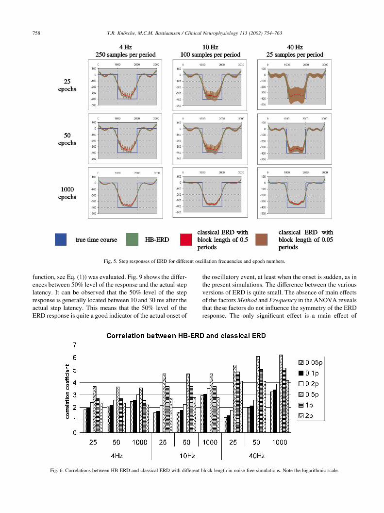
In Fig. 5, some of the computed step responses are

summarized. It can be seen that the time course is very

similar for all methods, except for a ringing effect that

occurs if the blocks are short with respect to the oscillation

period. This effect is greatly diminished, if more epochs are

taken into account. On the other hand, if the blocks are very

long (2 or 5 periods), the final height of the step is lower (not

shown in figure). HB-ERD and classical ERD with a block

length of 0.5 oscillation periods show the most similar

curves (see red and blue traces in Fig. 5). Fig. 6 demon-

strates the high similarity of different block-based ERD

variants with HB-ERD. Between classical ERD with block

length of 0.5 periods and HB-ERD, there is a correlation of

minimally 0.999.

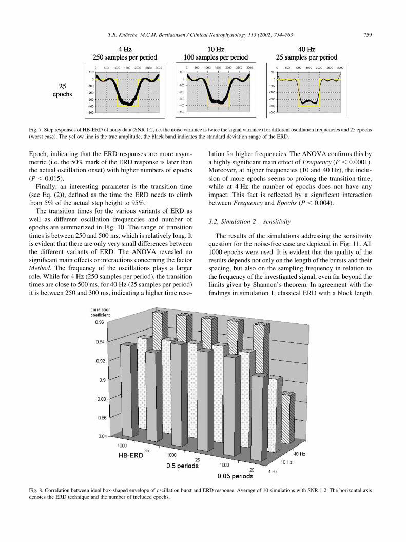
Fig. 7 additionally shows that the added noise does not

change the shape of the curve of the HB-ERD. The variation

between different noise realizations is relatively small, even

for only 25 epochs. The same was found for block-based

ERD.

The correlations between actual envelope and ERD

curves, averaged over 10 noise realizations, are given in

Fig. 8. The ANOVA on these correlation coefficients reveals

that there is an overall trend to higher correlations with

higher frequencies and (less clear) with more epochs. This

is manifested by significant main effects for Frequency ðP ,

0:0001Þ and for Epoch ðP , 0:025Þ. However, only for clas-

sical ERD with blocks of 0.05 periods and only for the 25

epochs case, this pattern is disturbed. In this case, higher

frequencies lead to lower correlations, which is probably

due to the presence of riding oscillations, as can be seen

in Fig. 5. This is expressed in significant interactions

Method £ Frequency, Epochs £ Frequency, and Method £

Epochs £ Frequency. (all P values ,0.0001).

In order to assess the relationship between the 50% level

of the step response and the latency of the actual step, the

parameter c (representing symmetry in the approximating


Fig. 4. Amplitudes of the test datasets for simulation 2 (sensitivity). The phase is random. The time differences are given relatively in terms of period length of

the oscillations.

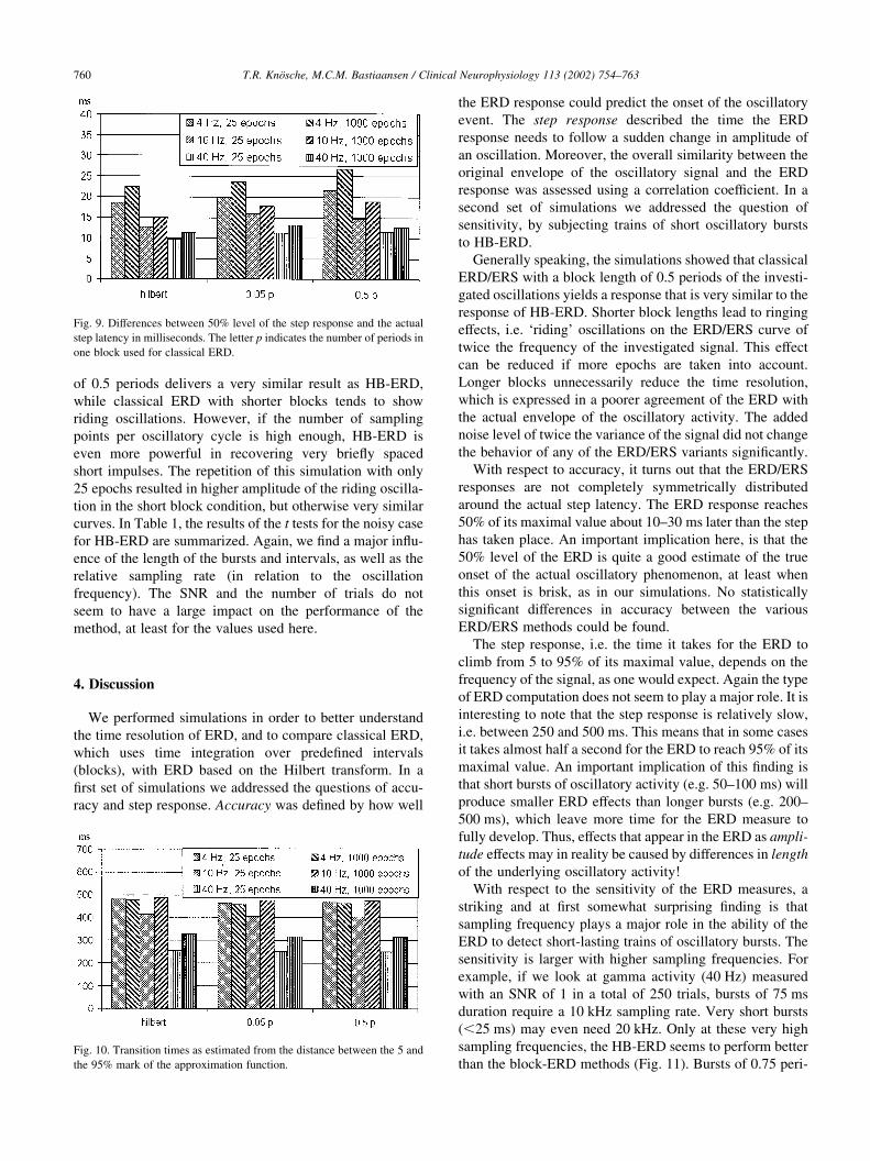
function, see Eq. (1)) was evaluated. Fig. 9 shows the differ-

ences between 50% level of the response and the actual step

latency. It can be observed that the 50% level of the step

response is generally located between 10 and 30 ms after the

actual step latency. This means that the 50% level of the

ERD response is quite a good indicator of the actual onset of

the oscillatory event, at least when the onset is sudden, as in

the present simulations. The difference between the various

versions of ERD is quite small. The absence of main effects

of the factors Method and Frequency in the ANOVA reveals

that these factors do not influence the symmetry of the ERD

response. The only significant effect is a main effect of


Fig. 6. Correlations between HB-ERD and classical ERD with different block length in noise-free simulations. Note the logarithmic scale.

Fig. 5. Step responses of ERD for different oscillation frequencies and epoch numbers.

Epoch, indicating that the ERD responses are more asym-

metric (i.e. the 50% mark of the ERD response is later than

the actual oscillation onset) with higher numbers of epochs

ðP , 0:015Þ.

Finally, an interesting parameter is the transition time

(see Eq. (2)), defined as the time the ERD needs to climb

from 5% of the actual step height to 95%.

The transition times for the various variants of ERD as

well as different oscillation frequencies and number of

epochs are summarized in Fig. 10. The range of transition

times is between 250 and 500 ms, which is relatively long. It

is evident that there are only very small differences between

the different variants of ERD. The ANOVA revealed no

significant main effects or interactions concerning the factor

Method. The frequency of the oscillations plays a larger

role. While for 4 Hz (250 samples per period), the transition

times are close to 500 ms, for 40 Hz (25 samples per period)

it is between 250 and 300 ms, indicating a higher time reso-

lution for higher frequencies. The ANOVA confirms this by

a highly significant main effect of Frequency ðP , 0:0001Þ.

Moreover, at higher frequencies (10 and 40 Hz), the inclu-

sion of more epochs seems to prolong the transition time,

while at 4 Hz the number of epochs does not have any

impact. This fact is reflected by a significant interaction

between Frequency and Epochs ðP , 0:004Þ.

3.2. Simulation 2 – sensitivity

The results of the simulations addressing the sensitivity

question for the noise-free case are depicted in Fig. 11. All

1000 epochs were used. It is evident that the quality of the

results depends not only on the length of the bursts and their

spacing, but also on the sampling frequency in relation to

the frequency of the investigated signal, even far beyond the

limits given by Shannon’s theorem. In agreement with the

findings in simulation 1, classical ERD with a block length


Fig. 8. Correlation between ideal box-shaped envelope of oscillation burst and ERD response. Average of 10 simulations with SNR 1:2. The horizontal axis

denotes the ERD technique and the number of included epochs.

Fig. 7. Step responses of HB-ERD of noisy data (SNR 1:2, i.e. the noise variance is twice the signal variance) for different oscillation frequencies and 25 epochs

(worst case). The yellow line is the true amplitude, the black band indicates the standard deviation range of the ERD.

of 0.5 periods delivers a very similar result as HB-ERD,

while classical ERD with shorter blocks tends to show

riding oscillations. However, if the number of sampling

points per oscillatory cycle is high enough, HB-ERD is

even more powerful in recovering very briefly spaced

short impulses. The repetition of this simulation with only

25 epochs resulted in higher amplitude of the riding oscilla-

tion in the short block condition, but otherwise very similar

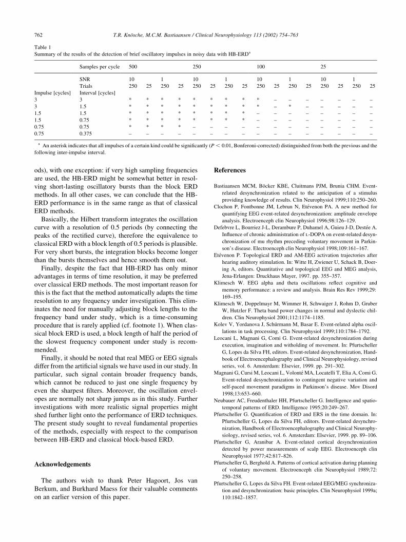
curves. In Table 1, the results of the t tests for the noisy case

for HB-ERD are summarized. Again, we find a major influ-

ence of the length of the bursts and intervals, as well as the

relative sampling rate (in relation to the oscillation

frequency). The SNR and the number of trials do not

seem to have a large impact on the performance of the

method, at least for the values used here.

4. Discussion

We performed simulations in order to better understand

the time resolution of ERD, and to compare classical ERD,

which uses time integration over predefined intervals

(blocks), with ERD based on the Hilbert transform. In a

first set of simulations we addressed the questions of accu-

racy and step response. Accuracy was defined by how well

the ERD response could predict the onset of the oscillatory

event. The step response described the time the ERD

response needs to follow a sudden change in amplitude of

an oscillation. Moreover, the overall similarity between the

original envelope of the oscillatory signal and the ERD

response was assessed using a correlation coefficient. In a

second set of simulations we addressed the question of

sensitivity, by subjecting trains of short oscillatory bursts

to HB-ERD.

Generally speaking, the simulations showed that classical

ERD/ERS with a block length of 0.5 periods of the investi-

gated oscillations yields a response that is very similar to the

response of HB-ERD. Shorter block lengths lead to ringing

effects, i.e. ‘riding’ oscillations on the ERD/ERS curve of

twice the frequency of the investigated signal. This effect

can be reduced if more epochs are taken into account.

Longer blocks unnecessarily reduce the time resolution,

which is expressed in a poorer agreement of the ERD with

the actual envelope of the oscillatory activity. The added

noise level of twice the variance of the signal did not change

the behavior of any of the ERD/ERS variants significantly.

With respect to accuracy, it turns out that the ERD/ERS

responses are not completely symmetrically distributed

around the actual step latency. The ERD response reaches

50% of its maximal value about 10–30 ms later than the step

has taken place. An important implication here, is that the

50% level of the ERD is quite a good estimate of the true

onset of the actual oscillatory phenomenon, at least when

this onset is brisk, as in our simulations. No statistically

significant differences in accuracy between the various

ERD/ERS methods could be found.

The step response, i.e. the time it takes for the ERD to

climb from 5 to 95% of its maximal value, depends on the

frequency of the signal, as one would expect. Again the type

of ERD computation does not seem to play a major role. It is

interesting to note that the step response is relatively slow,

i.e. between 250 and 500 ms. This means that in some cases

it takes almost half a second for the ERD to reach 95% of its

maximal value. An important implication of this finding is

that short bursts of oscillatory activity (e.g. 50–100 ms) will

produce smaller ERD effects than longer bursts (e.g. 200–

500 ms), which leave more time for the ERD measure to

fully develop. Thus, effects that appear in the ERD as ampli-

tude effects may in reality be caused by differences in length

of the underlying oscillatory activity!

With respect to the sensitivity of the ERD measures, a

striking and at first somewhat surprising finding is that

sampling frequency plays a major role in the ability of the

ERD to detect short-lasting trains of oscillatory bursts. The

sensitivity is larger with higher sampling frequencies. For

example, if we look at gamma activity (40 Hz) measured

with an SNR of 1 in a total of 250 trials, bursts of 75 ms

duration require a 10 kHz sampling rate. Very short bursts

(,25 ms) may even need 20 kHz. Only at these very high

sampling frequencies, the HB-ERD seems to perform better

than the block-ERD methods (Fig. 11). Bursts of 0.75 peri-


Fig. 9. Differences between 50% level of the step response and the actual

step latency in milliseconds. The letter p indicates the number of periods in

one block used for classical ERD.

Fig. 10. Transition times as estimated from the distance between the 5 and

the 95% mark of the approximation function.

ods of the signal (e.g. with a length of 18–20 ms for gamma

frequencies) can be reliably resolved. When more moderate

sampling rates are used, the different methods perform simi-

larly. The dependence of the detectability of short bursts on

the relative sampling rate (samples per period) can be attrib-

uted to the high frequencies that make up the sharp edges of

the burst envelope. A too low sampling rate causes the ERD

response not to follow the envelope closely enough and to

smooth out the bursts.

Summarizing, one can state that the claim made by

Clochon et al. (1996) that the HB-ERD has a millisecond

time resolution can be definitely rejected on the basis of the

present results. In terms of accuracy, HB-ERD is not super-

ior to classical ERD with optimum block length (0.5 peri-


Fig. 11. ERD results for brief oscillatory bursts. The bursts contain 3, 1.5, or 0.75 periods of the oscillation and are separated by 1 or 0.5 burst length. The

signals are sampled with 500, 250, 100, or 25 samples per period of the oscillation. The oscillation amplitude during the bursts is twice the amplitude between

them. The blue line indicates the true envelope of the burst signal.

ods), with one exception: if very high sampling frequencies

are used, the HB-ERD might be somewhat better in resol-

ving short-lasting oscillatory bursts than the block ERD

methods. In all other cases, we can conclude that the HB-

ERD performance is in the same range as that of classical

ERD methods.

Basically, the Hilbert transform integrates the oscillation

curve with a resolution of 0.5 periods (by connecting the

peaks of the rectified curve), therefore the equivalence to

classical ERD with a block length of 0.5 periods is plausible.

For very short bursts, the integration blocks become longer

than the bursts themselves and hence smooth them out.

Finally, despite the fact that HB-ERD has only minor

advantages in terms of time resolution, it may be preferred

over classical ERD methods. The most important reason for

this is the fact that the method automatically adapts the time

resolution to any frequency under investigation. This elim-

inates the need for manually adjusting block lengths to the

frequency band under study, which is a time-consuming

procedure that is rarely applied (cf. footnote 1). When clas-

sical block ERD is used, a block length of half the period of

the slowest frequency component under study is recom-

mended.

Finally, it should be noted that real MEG or EEG signals

differ from the artificial signals we have used in our study. In

particular, such signal contain broader frequency bands,

which cannot be reduced to just one single frequency by

even the sharpest filters. Moreover, the oscillation envel-

opes are normally not sharp jumps as in this study. Further

investigations with more realistic signal properties might

shed further light onto the performance of ERD techniques.

The present study sought to reveal fundamental properties

of the methods, especially with respect to the comparison

between HB-ERD and classical block-based ERD.

Acknowledgements

The authors wish to thank Peter Hagoort, Jos van

Berkum, and Burkhard Maess for their valuable comments

on an earlier version of this paper.

References

Bastiaansen MCM, Bocker KBE, Cluitmans PJM, Brunia CHM. Event-

related desynchronization related to the anticipation of a stimulus

providing knowledge of results. Clin Neurophysiol 1999;110:250–260.

Clochon P, Fontbonne JM, Lebrun N, Etevenon PA. A new method for

quantifying EEG event-related desynchronization: amplitude envelope

analysis. Electroenceph clin Neurophysiol 1996;98:126–129.

Defebvre L, Bourriez J-L, Derambure P, Duhamel A, Guieu J-D, Destee A.

Influence of chronic administration of l-DOPA on event-related desyn-

chronization of mu rhythm preceding voluntary movement in Parkin-

son’s disease. Electroenceph clin Neurophysiol 1998;109:161–167.

Etevenon P. Topological ERD and AM-EEG activation trajectories after

hearing auditory stimulation. In: Witte H, Zwiener U, Schack B, Doer-

ing A, editors. Quantitative and topological EEG and MEG analysis,

Jena-Erlangen: Druckhaus Mayer, 1997. pp. 355–357.

Klimesch W. EEG alpha and theta oscillations reflect cognitive and

memory performance: a review and analysis. Brain Res Rev 1999;29:

169–195.

Klimesch W, Doppelmayr M, Wimmer H, Schwaiger J, Rohm D, Gruber

W, Hutzler F. Theta band power changes in normal and dyslectic chil-

dren. Clin Neurophysiol 2001;112:1174–1185.

Kolev V, Yordanova J, Schurmann M, Basar E. Event-related alpha oscil-

lations in task processing. Clin Neurophysiol 1999;110:1784–1792.

Leocani L, Magnani G, Comi G. Event-related desynchronization during

execution, imagination and witholding of movement. In: Pfurtscheller

G, Lopes da Silva FH, editors. Event-related desynchronization, Hand-

book of Electroencephalography and Clinical Neurophysiology, revised

series, vol. 6. Amsterdam: Elsevier, 1999. pp. 291–302.

Magnani G, Cursi M, Leocani L, Volonte MA, Locatelli T, Elia A, Comi G.

Event-related desynchronization to contingent negative variation and

self-paced movement paradigms in Parkinson’s disease. Mov Disord

1998;13:653–660.

Neubauer AC, Freudenthaler HH, Pfurtscheller G. Intelligence and spatio-

temporal patterns of ERD. Intelligence 1995;20:249–267.

Pfurtscheller G. Quantification of ERD and ERS in the time domain. In:

Pfurtscheller G, Lopes da Silva FH, editors. Event-related desynchro-

nization, Handbook of Electroencephalography and Clinical Neurophy-

siology, revised series, vol. 6. Amsterdam: Elsevier, 1999. pp. 89–106.

Pfurtscheller G, Aranibar A. Event-related cortical desynchronization

detected by power measurements of scalp EEG. Electroenceph clin

Neurophysiol 1977;42:817–826.

Pfurtscheller G, Berghold A. Patterns of cortical activation during planning

of voluntary movement. Electroenceph clin Neurophysiol 1989;72:

250–258.

Pfurtscheller G, Lopes da Silva FH. Event-related EEG/MEG synchroniza-

tion and desynchronization: basic principles. Clin Neurophysiol 1999a;

110:1842–1857.


Table 1

Summary of the results of the detection of brief oscillatory impulses in noisy data with HB-ERDa

Samples per cycle 500 250 100 25

SNR 10 1 10 1 10 1 10 1

Trials 250 25 250 25 250 25 250 25 250 25 250 25 250 25 250 25

Impulse [cycles] Interval [cycles]

3 3 * * * * * * * * * – – – – – – –

3 1.5 * * * * * * * * * – * – – – – –

1.5 1.5 * * * * * * * * – – – – – – – –

1.5 0.75 * * * * * * * * – – – – – – – –

0.75 0.75 * * * * – – – – – – – – – – – –

0.75 0.375 – – – – – – – – – – – – – – – –

a An asterisk indicates that all impulses of a certain kind could be significantly (P , 0:01, Bonferoni-corrected) distinguished from both the previous and the

following inter-impulse interval.

Pfurtscheller G, Lopes da Silva FH, editors. Event-related desynchroniza-

tion Handbook of Electroencephalography and Clinical Neurophysiol-

ogy, revised series, vol. 6. Amsterdam: Elsevier, 1999b.

Pfurtscheller G, Neuper C. Event-related synchronization of mu rhythm in

the EEG over the cortical hand area in man. Neurosci Lett 1994;174:

93–96.

Pfurtscheller G, Stancak A, Neuper C. Post-movement beta synchroniza-

tion: a correlate of an idling motor area? Electroenceph clin Neurophy-

siol 1996;98:281–293.

Yordanova J, Kolev V. Event-related alpha oscillations are functionally

related with P300 during information processing. NeuroReport 1998;9:

3159–3164.


On the time resolution of event-related desynchronization: a simulation study

Documents

Transcript of On the time resolution of event-related desynchronization: a simulation study