arX

iv:h

ep-t

h/93

0109

9v3

26

Feb

1993

CTP TAMU–4/93

Preprint-KUL-TF-93/2

hep-th/9301099

January 1993

On the Spectrum and Scattering of W3 Strings

H. Lu, C.N. Pope,∗ S. Schrans⋄ and X.J. Wang

Center for Theoretical Physics, Texas A&M University,

College Station, TX 77843–4242, USA.

ABSTRACT

We present a detailed investigation of scattering processes in W3 stringtheory. We discover further physical states with continuous momentum,which involve excitations of the ghosts as well as the matter, and use themto gain a better understanding of the interacting theory. The scatteringamplitudes display factorisation properties, with states from the differentsectors of the theory being exchanged in the various intermediate channels.We find strong evidence for the unitarity of the theory, despite the unusualghost structure of some of the physical states. Finally, we show that byperforming a transformation of the quantum fields that involves mixing theghost fields with one of the matter fields, the structure of the physical statesis dramatically simplified. The new formalism provides a concise frameworkwithin which to study the W3 string.

∗ Supported in part by the U.S. Department of Energy, under grant DE-FG05-91ER40633.⋄ Onderzoeker I.I.K.W.; On leave of absence from the Instituut voor Theoretische Fysica,

K.U. Leuven, Belgium. Address after March 1, 1993: Koninklijke/Shell-Laboratorium,Amsterdam (Shell Research B.V.), Badhuisweg 3, 1031 CM Amsterdam, The Netherlands.

1. Introduction

Since the discovery of W3 symmetry [1] in two-dimensional field theories much work has

been carried out on the construction of W3-string theories [2–12]. Most of these efforts have

been concerned with the understanding of their physical spectra [2–10,12]. Until recently,

attention had been focussed on physical states with standard ghost structure, which are

direct analogues of the physical states in the usual 26-dimensional bosonic string. It has

been recently realised that there are also physical states with non-standard ghost structure

in the W3 string, i.e. states that involve excitations of the ghost fields as well as the matter

fields [13,9–12]. Unlike the two-dimensional string, where states of this kind occur too [14,15],

they exist not only in the two-scalar W3 string where the momenta are discrete, but also in

the multi-scalar W3 string where the momenta are in general continuous. The occurrence of

states involving excitations of the ghost fields in the physical spectrum is rather unusual in

a gauge theory, and normally one might expect that it would be associated with a violation

of unitarity. However, as was discussed in [11], and will be explored further in this paper,

it seems that these states are unitary, and furthermore, they are an essential ingredient of

the W3 string. In fact, as we recently showed [11], the existence of physical states with non-

standard ghost structure resolves the long-standing puzzle of how to introduce interactions

in the W3 string.

As in ordinary string theory, interactions have to be introduced by hand. The guiding

principle that determines acceptable interactions is that they should respect the symmetries

of the theory. This means in the present context that they should lead to BRST-invariant

scattering amplitudes. The stumbling-block to introducing interactions in the W3 string was

that for a long time only the physical states with standard ghost structure were known,

and with these it appears to be impossible to write down any non-vanishing BRST-invariant

amplitude. The reason for this is that these physical states, and indeed all physical states

in the W3 string, have specific values of momentum in a particular “frozen” direction, and

the particular values that occur for the states with standard ghost structure imply that

momentum conservation in this direction cannot be satisfied in interactions.

In [11], we presented a procedure for building gauge-invariant scattering amplitudes in

the W3 string. An essential aspect is that non-vanishing scattering amplitudes necessarily

involve external physical states with non-standard ghost structure. The problem with mo-

mentum conservation in the frozen direction is avoided because these states have different

values of frozen momentum from those of the states with standard ghost structure. In this

paper we shall review and elaborate on this procedure, resolve some open problems in [11],

and begin the unravelling of the general structure of W3-string scattering.

The paper is organised as follows. Section 2 contains a summary of the main results in

[11] and outlines several issues that we shall explore further in this paper.

2

We begin section 3 by finding new physical states of the W3 string; they have higher

levels, and lower ghost numbers, than the ones that were known previously. All the physical

states we know fall into two categories: those with continuous on-shell spacetime momentum,

and those where the on-shell spacetime momentum can only take a discrete value (in fact,

zero). The new physical states enable us to gain a better understanding of the interactions of

the W3 string. In particular, we are now able to construct certain interactions that could not

have been obtained with the physical states of [11] alone. We then explain how the physical

states can be organised into multiplets and discuss their structure in detail. One of the main

features that emerges from the examples of physical states with continuous momentum that

we have constructed is that they all admit an effective spacetime interpretation. By this we

mean that a physical state of this kind factorises into a direct product of a piece involving the

ghost fields together with the frozen coordinate, and another piece involving the remaining

coordinates which can then be viewed as the coordinates of the target spacetime. Moreover,

we find that from the effective spacetime point of view, these states fall into three sectors,

with effective conformal dimension Leff0 = 1, 15

16and 1

2.

In section 4 we use the known physical states to build new four-point and five-point

scattering amplitudes. One of these is a four-point function for four physical states in the

Leff0 = 1 sector. It provides a useful non-trivial check of our procedure, since it should, and

indeed does, agree with the corresponding result in ordinary bosonic string theory (at tree

level). We also show that physical states in the Leff0 = 15

16sector play a special role in the

theory in that there are only very limited possibilities for them to interact with other states.

Specifically, we find that no more than two of the physical states in a non-vanishing N -point

function can have Leff0 = 15

16 .

Section 5 is divided into two subsections. In the first we make some general observations

about the physical spectrum of the W3 string and derive necessary conditions for the level

numbers and momenta in the frozen direction of physical states which admit an effective

spacetime interpretation and have Leff0 taking values in the set {1, 15

16, 1

2}. In the second

subsection we consider the unitarity of the theory. We show that if all the physical states

with continuous momentum indeed admit an effective spacetime interpretation and have the

above values of Leff0 , then the W3 string is unitary. Further evidence for unitarity comes

from looking at the residues of the poles of the scattering amplitudes.

Motivated by the fact that all the continuous-momentum physical states known so far

admit an effective spacetime interpretation, in section 6 we introduce a formalism that

exploits this. It consists of making a certain transformation of the quantum fields, which

mixes the ghost fields with the frozen coordinate. It is a canonical transformation, in the

sense that the new fields satisfy the same set of operator-product expansions as the original

ones. In terms of these redefined fields, the known physical operators acquire a remarkably

simple form. A striking example is provided by a level 8 physical operator, which reduces

from 82 terms to 4 after transforming to the new fields. Moreover, this formalism will make

3

more transparent some of the features of the W3 string that we have encountered in this

paper. The simplification achieved by this transformation is highly suggestive that the new

formalism is the appropriate one for describing the W3 string.

The paper ends with concluding remarks in section 7.

2. A review of the W3 string

In this section we review the procedure and main results of [11]. In order to make the

present paper as self-contained as possible, and in order to establish notation, a certain

amount of repetition is unavoidable.

The key ingredient for determining the physical spectrum of the W3 string is the con-

struction of the BRST operator [16], which is given by

QB =

∮dz

[c (T + 1

2Tgh) + γ (W + 1

2Wgh)

], (2.1)

and is nilpotent provided that the matter currents T and W generate the W3 algebra with

central charge c = 100, and that the ghost currents are chosen to be

Tgh = −2b ∂c − ∂b c − 3β ∂γ − 2∂β γ , (2.2)

Wgh = −∂β c − 3β ∂c − 8261

[∂(b γ T ) + b ∂γ T

]

+ 251566

(2γ ∂3b + 9∂γ ∂2b + 15∂2γ ∂b + 10∂3γ b

), (2.3)

where the ghost-antighost pairs (c, b) and (γ, β) correspond respectively to the T and W

generators. A matter realisation of W3 with central charge 100 can be given in terms of

n ≥ 2 scalar fields, as follows [17]:

T = −12(∂ϕ)2 − Q∂2ϕ + T eff ,

W = − 2i√261

[13(∂ϕ)3 + Q∂ϕ∂2ϕ + 1

3Q2∂3ϕ + 2∂ϕT eff + Q∂T eff],

(2.4)

where Q2 = 498 and T eff is an energy-momentum tensor with central charge 51

2 that commutes

with ϕ. Since T eff has a fractional central charge, it cannot be realised simply by taking free

scalar fields. We can however use d scalar fields Xµ with a background-charge vector aµ:

T eff = −12∂Xµ∂Xµ − iaµ∂2Xµ, (2.5)

with aµ chosen so that 512

= d − 12aµaµ [17].

Physical states are by definition states that are annihilated by the BRST operator (2.1)

but that are not BRST trivial. Such states with standard ghost structure are of the form:

∣∣χ⟩

=∣∣−−

⟩⊗

∣∣ϕ , X⟩. (2.6)

4

Here∣∣−−

⟩is the standard ghost vacuum, given by

∣∣−−⟩

= c1γ1γ2

∣∣0⟩. (2.7)

The SL(2, C) vacuum satisfies

cn

∣∣0⟩

= 0, n ≥ 2; bn

∣∣0⟩

= 0, n ≥ −1, (2.8a)

γn

∣∣0⟩

= 0, n ≥ 3; βn

∣∣0⟩

= 0, n ≥ −2. (2.8b)

The antighost fields b, β have ghost number G = −1, and the ghost fields c, γ have ghost

number G = 1.∗

For standard states of the form (2.6), the condition of BRST invariance becomes [16]:

(L0 − 4)∣∣ϕ , X

⟩= 0,

W0

∣∣ϕ , X⟩

= 0,

Ln

∣∣ϕ , X⟩

= Wn

∣∣ϕ , X⟩

= 0, n ≥ 1.

(2.9)

The consequences of these physical-state conditions have been studied in detail in various

papers [3–8,10]. The main features that emerge are the following. There are two kinds of

excited states, namely those for which there are no excitations in the ϕ direction, and those

where ϕ is excited too. The latter states are all BRST trivial, as has been discussed in

[6,8,18]. For the former, we may write∣∣ϕ , X

⟩as

∣∣ϕ , X⟩

= eβϕ(0)∣∣phys

⟩eff

, (2.10)

where∣∣phys

⟩eff

involves only the Xµ fields and not ϕ. (There will be no confusion between

the frozen momentum β and the spin-3 antighost β.) The physical-state conditions (2.9)

imply that

(β + Q)(β + 67Q)(β + 8

7Q) = 0, (2.11)

together with the effective physical-state conditions:

(Leff0 − ∆)

∣∣phys⟩eff

= 0,

Leffn

∣∣phys⟩eff

= 0, n ≥ 1.(2.12)

The value of the effective intercept ∆ is 1 when β = −67Q or −8

7Q, and it equals 1516

when β = −Q. Thus these states of the W3 string are described by two effective Virasoro-

string spectra, for an effective energy-momentum tensor T eff with central charge c = 512

and

intercepts ∆ = 1 and ∆ = 1516 . The first of these gives a mass spectrum similar to an ordinary

∗ For states, we follow the convention in [11] that the ghost vacuum∣∣−−

⟩has ghost number G = 0,

which means that the SL(2, C) vacuum∣∣0

⟩has ghost number G = −3. This implies that physical states of

ghost number G are obtained by acting on∣∣0

⟩with operators of ghost number (G + 3).

5

string, with a massless vector at level 1, whilst the second gives a spectrum of purely massive

states [5,6].

As we have indicated in the introduction, the W3-string spectrum is much richer than

simply that of the standard physical states we have discussed so far. Although the classifica-

tion of physical states with non-standard ghost structure is as yet incomplete, some classes

of such states have been found [9,11,12]. They contain excitations of the ghost and antighost

fields as well as the matter fields. The level number ℓ of these states is defined with respect

to the ghost vacuum∣∣−−

⟩given in (2.7). Thus, for example, the SL(2, C) vacuum

∣∣0⟩

has

level number ℓ = 4 and ghost number G = −3, since it can be written as β−2β−1b−1

∣∣−−⟩. It

is straightforward to see that at level ℓ, the allowed ghost numbers of states (not necessarily

physical) lie in the interval

1 −[√

4ℓ + 1]≤ G ≤ 1 +

[√4ℓ + 1

], (2.13)

where[a]

denotes the integer part of a.

All the physical states in the W3 string occur in multiplets [9,11]. The members of a

multiplet are obtained by (repeatedly) acting with the G = 1 operators aϕ ≡ [QB, ϕ] and

aXµ ≡ [QB , Xµ] on a physical state that we call a prime state. Until now the known examples

of prime states occurred either at ghost number G = 0 (in the case of states with standard

ghost structure), or at G = −1 or G = −3 (in the case of states with non-standard ghost

structure). The corresponding operators have ghost numbers G = 3, G = 2 or G = 0. All

physical states in the W3 string occur with ϕ momentum frozen to specific values. Examples

of physical states at level ℓ = 0, 1, 2, 3 were given in [11] and used for calculating scattering

amplitudes. All the prime operators of [11] have an effective spacetime interpretation, in

the sense that they can be written as products of the form V = U(gh,ϕ) Ueff , where U(gh,ϕ)

involves only the ghosts and the ϕ field, and Ueff involves only the effective spacetime

coordinates Xµ. We have already seen from (2.6) and (2.10) that states with standard ghost

structure give physical operators of this form, with Ueff having effective intercepts Leff0 = 1

or 1516 as measured by T eff . The prime operators with non-standard ghost structure discussed

in [11] can have three possible values for Leff0 , namely 1, 15

16or 1

2. In section 3 we shall find

new prime states at ℓ = 4, G = −2; ℓ = 5, G = −2; and ℓ = 8, G = −3.∗ They again

all admit an effective spacetime interpretation, with the same three values of Leff0 . By using

these new states in scattering calculations, we shall be able to clarify some unresolved issues

in [11]. We shall also describe the structure of the multiplets in the multi-scalar W3 string.

As we shall see, for the physical states described above, the ghost boosters aϕ and aXµ

generate a quartet from a given prime state.

∗ In [11], a physical state at ℓ = 3, G = −1 given by the operator (A.12) of [11] was inadvertentlydescribed as a prime state. In fact the prime state at this level occurs at G = −2, and corresponds to theoperator given in (A.7) of this paper; the state used in [11] is obtained by acting with the ghost boosters aϕ

and aXµ on this prime state.

6

Scattering amplitudes are obtained by integrating over the worldsheet coordinates of

physical operators in correlation functions. For the W3 string the correlation functions are,

by definition, given by functional integrals over all the quantum fields of the theory, namely

the ghosts b, c, β and γ, the ϕ field, and the effective spacetime coordinates Xµ. These

functional integrals can, as usual, be conveniently calculated by using the techniques of

conformal field theory.

A physical operator, denoted generically by V (z), is by definition a non-trivial BRST-

invariant operator that gives rise to the physical state V (0)∣∣0

⟩. In particular, it has conformal

dimension 0, as measured by the total energy-momentum tensor T tot = T +Tgh. (Note that

V (z) includes ghosts as well as the matter fields.) In an N -point scattering amplitude one

can use the SL(2, C) invariance of∣∣0

⟩to fix the worldsheet coordinates of three of the

operators in the correlation function, leaving (N − 3) coordinates over which to integrate.

For conformal covariance one must integrate over operators of dimension 1. As in string

theory [19], this can be achieved by making the replacement

V (z) → 1

2πi

∮

z

dw b(w)V (z), (2.14)

where the subscript on the contour integral indicates that it should be evaluated around a

path enclosing z. In fact this procedure not only preserves the projective structure but also

gives scattering amplitudes that are invariant under the BRST transformations generated

by (2.1) [11]. This is because the BRST variation of the right-hand side of (2.14) is a total

derivative. Note that one cannot use the spin-3 antighost β in place of b in (2.14), since it

would not give BRST-invariant amplitudes.

In the ordinary 26-dimensional bosonic string, the physical operators all have the form

V (z) =(c U

)(z) (or its conjugate,

(∂c c U

)(z)), where U(z) involves only the coordinates

Xµ but no ghosts. If the replacement (2.14) were not made in (N ≥ 4)-point functions (and

accordingly, the corresponding worldsheet coordinate were left unintegrated), the results

would certainly be BRST invariant. However, they would trivially be zero, since the non-

zero ghost inner product in string theory is⟨0∣∣∂2c ∂c c

∣∣0⟩

[19]. In the W3 string, on the

other hand, physical operators do not all have the standard ghost structure, so it is no

longer a priori obvious that the replacement (2.14) is required in order to get non-zero

results for BRST-invariant (N ≥ 4)-point scattering amplitudes. Nevertheless, it seems that

the corresponding correlation functions in the W3 string vanish unless the replacement (2.14)

is made, as we shall discuss in section 6. (The situation is different if physical states with

discrete effective-spacetime momentum are involved; see section 4.)

In order to identify which correlation functions might be non-vanishing, it is useful first

to consider two necessary conditions [11]. If these conditions are satisfied, then it becomes

a matter of more detailed calculation to determine the result. The first of the necessary

conditions is that the total ghost structure of the product of operators in the correlation

7

function should be appropriate. Specifically, the non-vanishing ghost inner product in the

W3 string is given by

1 =⟨0∣∣c−1c0c1 γ−2γ−1γ0γ1γ2

∣∣0⟩

= 1576

⟨0∣∣∂2c ∂c c ∂4γ ∂3γ ∂2γ ∂γ γ

∣∣0⟩

. (2.15)

(See [11] for a more detailed discussion.) Note that in particular the total ghost number of

the operators in a non-vanishing correlator must be 3 + 5 = 8.

The second of the necessary conditions for obtaining a non-vanishing correlation function

is that momentum conservation must be satisfied. Owing to the presence of the background

charges, this implies that we must have∑N

i=1 pµi = −2aµ in the effective spacetime, together

withN∑

i=1

βi = −2Q (2.16)

in the ϕ direction. For states of continuous spacetime momentum pµ, as indeed we have in

the multi-scalar W3 string, momentum conservation in the Xµ directions can be straightfor-

wardly satisfied. However, the momentum β in the ϕ direction can only take specific frozen

values in physical states. (For physical states with standard ghost structure this follows from

(2.11); it is true also for states with non-standard ghost structure, as we shall see again in

the next section.) Thus it is in general non-trivial to satisfy momentum conservation in the

ϕ direction. Note that (2.16) is an extremely restrictive condition; indeed it implies that

(N ≥ 3)-point correlation functions built exclusively from physical operators of standard

ghost structure will vanish, as may be seen from (2.11). It is worth emphasising that even

though ϕ does not admit the interpretation of being an observable spacetime coordinate,

the functional integration over it, and in particular over its zero-mode, determines a very

stringent W3 selection rule [11].

Using the procedure outlined above, we calculated various three-point and four-point

functions in [11], with the physical states given therein. A number of patterns emerged, which

we shall be able to develop further with the results of the present paper. In particular, it was

found that physical states seem to be characterised by their effective spacetime structure, in

the sense that physical states with the same Leff0 values but different ghost and ϕ dependence

give identical results in correlation functions, modulo an overall constant factor. This factor

depends on the normalisation of the states, and furthermore would be zero if, for example,

a selection rule such as (2.16) forbade a particular interaction.

It was found in [11] that non-vanishing three-point functions can occur for physical

operators with Leff0 values of {1, 1, 1}, {15

16, 15

16, 1}, {1

2, 1

2, 1} and {15

16, 15

16, 1

2}. All

other three-point functions vanish. These results for three-point functions are in one-to-one

correspondence with the fusion rules of the two-dimensional Ising model, if one associates the

Leff0 = 1 sector with the identity operator 1, the Leff

0 = 1516 sector with the spin operator σ, and

the Leff0 = 1

2 sector with the energy operator ε. This makes more precise the numerological

8

connection between W3 strings and the Ising model which emerges from the analysis of the

spectrum [3,6,10]. In particular, the central charge of the effective energy-momentum tensor

is 512 = 26− 1

2 , where 26 is the critical central charge of the usual bosonic string, and 12 is the

central charge of the Ising model; moreover, the set of Leff0 values {1, 15

16, 1

2} can be written

as 1 − ∆min, where 1 is the intercept of the usual bosonic string and ∆min takes the values

of the dimensions of the primary fields {1, σ, ε} of the Ising model.

One of the interesting results of [11] is that this connection between the W3 string and

the Ising model does not go both ways in higher-point functions. In particular, it was shown

in [11] that the selection rule (2.16) forbids the existence of a four-point function for four

physical operators with Leff0 = 15

16 , even though the four-point function⟨σ σ σ σ

⟩is non-

vanishing in the Ising model. We shall find further indications in section 4 from five-point

and six-point functions that the Leff0 = 15

16 sector plays a special role in the W3 string.

One of the general features that we observed in [11] is that four-point functions in the W3

string exhibit a duality property, which means that they can be interpreted in terms of

underlying three-point functions, with sets of intermediate states being exchanged in the s,

t or u channels. In this paper we shall illustrate this factorisation property for a five-point

function too.

3. New physical states and the multiplet structure

In this section, we shall construct some new physical states of the W3 string with non-

standard ghost structure. These are prime states at levels ℓ = 4 and 5, with ghost number

G = −2. We shall use these, and an ℓ = 8, G = −3 prime state which was found in [12], to

calculate more scattering amplitudes in the next section. In particular, the ℓ = 5 prime state

enables us to obtain a non-vanishing four-point function with four Leff0 = 1 operators, which

does not exist for the states given in [11]. The above states will provide more evidence for

the observation that physical states appear to be characterised by their effective spacetime

structures. We shall also investigate the multiplet structures generated by the action of the

ghost boosters aϕ and aXµ .

Until now, prime states have been discovered at ghost number G = 0 for states with

standard ghost structure, and at G = −1 and G = −3 in the case of states with non-standard

ghost structure. The two new prime states that we shall construct in this section occur at

G = −2, and thus are of a different kind.

The general procedure that we use for finding physical states is as follows. At a given,

fixed, level number ℓ and ghost number G we write down the most general state, as a sum

of all nG possible structures with arbitrary coefficients gi. Requiring BRST invariance leads

to nG+1 equations for the gi’s, giving mG independent solutions. There are nG−1 − mG−1

BRST-trivial states at ghost number G, where mG−1 denotes the number of BRST-invariant

states at ghost number G − 1. The number of BRST-nontrivial physical states at ghost

9

number G is therefore given by mG − (nG−1 − mG−1). Thus at a given level number ℓ we

may start from the lowest ghost number given by (2.13), and systematically work up to the

highest ghost number allowed by (2.13), finding all the non-trivial physical states at that

level. This is quite a tedious process, which is best performed with the aid of a computer.

Applying this procedure at level 4, we have found a physical state at G = −2, with ϕ

momentum β = 17Q. The general solution has three parameters which means, since there

are two BRST-trivial structures coming from QB acting on the two structures at G = −3,

that there is one non-trivial solution at G = −2. The two trivial parameters may be used

in order to give the physical state a convenient form. In fact, it turns out that they may

be chosen so as to remove all terms involving excitations of the spacetime coordinates, Xµ,

and thus the state acquires an effective spacetime interpretation, as a tachyon. The explicit

form of the corresponding physical operator, which has ghost number G = 1, is given in the

appendix in (A.8). For the amplitudes that we shall be concerned with in this paper, only

two of its thirteen terms contribute. They are

V115/16[

17Q, p] = − 3

16

√29 i

(3√

2 c β γ + 4∂ϕ c + · · ·)e

17

Qϕeip·X , (3.1)

where the effective spacetime momentum pµ satisfies the mass-shell condition

12pµ(pµ + 2aµ) = 15

16. (3.2)

In (3.1) we have used the notation of [11], where a physical operator V with ghost num-

ber G, Leff0 = ∆ and momentum (β, pµ) is denoted by VG

∆[β, p]. The operator (3.1) is a

representative of a tachyon of the Leff0 = 15

16sector of the W3 string. The operator eip·X

may be replaced by an arbitrary excited effective physical operator R(∂Xµ)eip′·X with the

same Leff0 value. This allows the construction of new physical states at higher levels with

Xµ excitations, that have an interpretation as excited effective spacetime states.

At level 5, we have found another new physical state at G = −2, with ϕ momentum

β = 27Q. Again we can use the freedom to add BRST-trivial terms so as to give the state

an effective spacetime interpretation, as a tachyon. The corresponding physical operator is

given in (A.9). For the amplitudes that we shall be concerned with in this paper, only 5 of

its 32 terms contribute, namely

V11[

27Q, p] = 1

20

√29 i

(6√

2 c ∂β γ − 3√

2 c β ∂γ + 12∂ϕ c β γ

+ 4√

2 ∂ϕ ∂ϕ c + 2∂2ϕ c + · · ·)e

27Qϕeip·X ,

(3.3)

where the effective spacetime momentum pµ satisfies the mass-shell condition

12pµ(pµ + 2aµ) = 1 . (3.4)

10

This operator is a representative of an effective tachyon of the Leff0 = 1 sector. Again, one

can replace eip·X by an arbitrary excited effective-spacetime physical operator with the same

Leff0 value.

The third physical state that we shall be using in this paper, and that was not given in

[11], occurs at level 8 with ghost number G = −3 and ϕ momentum β = 47Q; it was found

in [12]. Once more, the freedom of adding BRST trivial parts can be used to remove all

excitations in the Xµ directions, thus giving it the interpretation of an effective spacetime

tachyon. As such it is a representative of the Leff0 = 1

2 sector. It has 82 terms, and is given

in (A.10). In fact, for the scattering amplitudes that we shall calculate in the next section,

only four of those terms contribute to the result, namely

V01/2[

47Q, p] =

(∂ϕ c ∂β + 3

√2 c ∂β β γ − 3∂2ϕ c β − 3

4

√2 c ∂2β + · · ·

)e

47Qϕeip·X , (3.5)

where12pµ(pµ + 2aµ) = 1

2. (3.6)

The fact that only the small subsets of terms (3.1), (3.3) and (3.5) contribute in scattering

amplitudes involving the physical operators (A.8), (A.9) and (A.10) respectively suggests

that there is a great deal of redundancy in the formalism describing the W3 string. In

section 6, we shall introduce a new formalism that removes this redundancy.

The new physical operators that we have presented here have lower ghost numbers than

any of those used in [11]. Specifically, (A.8) and (A.9) have G = 1, and (A.10) has G = 0. An

important consequence of this is that it enables us to obtain non-vanishing N -point functions

for arbitrarily large N , whereas the physical operators of [11] only allowed their construction

for N ≤ 5. This is because the total ghost number of operators in a non-vanishing N -

point function must be equal to 8, and the insertion of many operators of the form (2.14)

will rapidly cause this number to be exceeded unless the physical operators V have ghost

numbers ≤ 1. We shall discuss this further at the end of section 4. This completes our

discussion of new prime states of the W3 string with continuous on-shell momenta.

Let us now turn our attention to the structure of the multiplets generated by the action

of the ghost boosters aϕ and aXµ on prime states. The explicit form of the ghost boosters

is given in [9] for the two-scalar W3 string and the generalisation to the multi-scalar case

is immediate. They are given in an alternative formulation in (6.21). Although we do not

have a general proof, we have checked the structure of the multiplets in several examples.

Acting on a prime state∣∣G

⟩at ghost number G with the (d + 1) ghost boosters, we obtain

just two independent non-trivial physical states at ghost number (G+1): aϕ

∣∣G⟩

=∣∣G+1

⟩1

and aXµ

∣∣G⟩

= (pµ + aµ)∣∣G + 1

⟩2. The fact that aXµ

∣∣G⟩

gives only one non-trivial state

rather than d is quite surprising and results in a much simpler multiplet structure than one

might have expected (we shall return to this point in section 6). The multiplet is completed

by a single non-trivial state∣∣G + 2

⟩obtained by acting either with aϕ on

∣∣G + 1⟩2

or with

11

aXµ on∣∣G + 1

⟩1. Thus it seems from our examples that each prime state

∣∣G⟩

gives rise to a

quartet of physical states {∣∣G

⟩,

∣∣G + 1⟩1,

∣∣G + 1⟩2,

∣∣G + 2⟩}. The structure is reminiscent

of an N = 2 supermultiplet.

As discussed in [9,11], each physical state at ghost number G and momentum (β, pµ) has

a conjugate partner at ghost number (2 − G) and momentum (−2Q − β,−2aµ − pµ). Thus

associated with each prime state is a quartet and a conjugate quartet of physical states.

We have already remarked that for all the known examples, prime states either auto-

matically have, or can be given, an effective spacetime interpretation. Remarkably, in all the

examples we have checked, the freedom to add BRST-trivial parts is precisely sufficient to

enable the boosted members of a multiplet to acquire an effective spacetime interpretation

too. In one of our examples, the prime state involved an excited effective spacetime part,

indicating that this effective spacetime interpretation is universal, and not just confined to

effective tachyonic states.

These considerations lead us to conjecture that all the physical states (with continuous

on-shell spacetime momentum pµ — see below) in the W3 string admit an effective spacetime

interpretation, i.e. they can all be written in the form

∣∣ghost + ϕ⟩⊗

∣∣effective spacetime⟩

. (3.7)

We shall sharpen this conjecture in section 6. Moreover, we conjecture that the effective

intercepts of all these physical states take values in the set {1, 1516 , 1

2}.∗

The above discussion of the effective-spacetime interpretation of physical states, and

their multiplet structure, applies for all physical states with continuous on-shell spacetime

momentum pµ. There are, however, additional physical states in the spectrum of the multi-

scalar W3 string that occur only for fixed values of pµ. In fact, in all the examples we know,

these discrete states occur with pµ = 0. The simplest example is provided by the SL(2, C)

vacuum,∣∣0

⟩= β−2β−1b−1

∣∣−−⟩, which is a level ℓ = 4 state with ghost number G = −3. We

shall adopt the notation DG[β] to denote the physical operator with ghost number G and ϕ

momentum β that gives a discrete state with ghost number (G − 3). Thus∣∣0

⟩corresponds

to the operator D0[0] = 1.

∗ In [13], physical states at ℓ = 2, G = 2 in the two-scalar W3 string were discussed, corresponding toan operator of the form ∂3c c ∂2γ ∂γ γeβ1ϕ1eβ2ϕ2 . This is annihilated by QB provided that the exponentialshave total conformal weight 2. However, contrary to what is asserted in [13], this state is in general BRSTtrivial, except for three values of (β1, β2). Two of these values, (− 12

7 Q,− 127 a) and (− 12

7 Q,− 27a), correspond

to states with Leff0 = 1

2 which generalise to an Leff0 = 1

2 state in the multi-scalar W3 string. (In fact this isthe conjugate of one of the quartet members from the prime state given by V

21/2[− 2

7Q, p] in formula (A.6).)

The third momentum value, (−Q,− 177 a), corresponds to a state with Leff

0 = − 1716 that does not generalise to

the multi-scalar W3 string. Our conjecture that the effective intercept values are {1, 1516 , 1

2} relates to thephysical states of the multi-scalar W3 string, and thus the Leff

0 = − 1716 state does not contradict it.

12

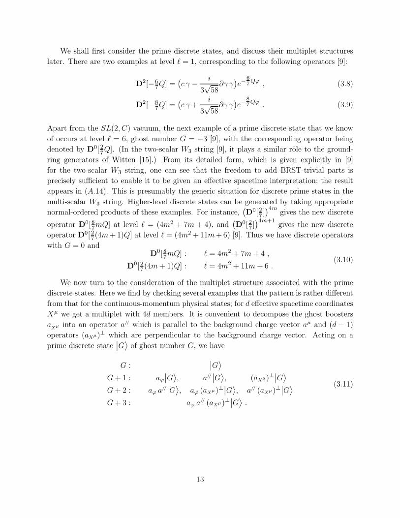
We shall first consider the prime discrete states, and discuss their multiplet structures

later. There are two examples at level ℓ = 1, corresponding to the following operators [9]:

D2[−67Q] =

(c γ − i

3√

58∂γ γ

)e−

67Qϕ , (3.8)

D2[−87Q] =

(c γ +

i

3√

58∂γ γ

)e−

87Qϕ . (3.9)

Apart from the SL(2, C) vacuum, the next example of a prime discrete state that we know

of occurs at level ℓ = 6, ghost number G = −3 [9], with the corresponding operator being

denoted by D0[27Q]. (In the two-scalar W3 string [9], it plays a similar role to the ground-

ring generators of Witten [15].) From its detailed form, which is given explicitly in [9]

for the two-scalar W3 string, one can see that the freedom to add BRST-trivial parts is

precisely sufficient to enable it to be given an effective spacetime interpretation; the result

appears in (A.14). This is presumably the generic situation for discrete prime states in the

multi-scalar W3 string. Higher-level discrete states can be generated by taking appropriate

normal-ordered products of these examples. For instance,(D0[2

7])4m

gives the new discrete

operator D0[87mQ] at level ℓ = (4m2 + 7m + 4), and(D0[27 ]

)4m+1gives the new discrete

operator D0[27(4m + 1)Q] at level ℓ = (4m2 + 11m + 6) [9]. Thus we have discrete operators

with G = 0 andD0[87mQ] : ℓ = 4m2 + 7m + 4 ,

D0[27(4m + 1)Q] : ℓ = 4m2 + 11m + 6 .

(3.10)

We now turn to the consideration of the multiplet structure associated with the prime

discrete states. Here we find by checking several examples that the pattern is rather different

from that for the continuous-momentum physical states; for d effective spacetime coordinates

Xµ we get a multiplet with 4d members. It is convenient to decompose the ghost boosters

aXµ into an operator a// which is parallel to the background charge vector aµ and (d − 1)

operators (aXµ)⊥ which are perpendicular to the background charge vector. Acting on a

prime discrete state∣∣G

⟩of ghost number G, we have

G :∣∣G

⟩

G + 1 : aϕ

∣∣G⟩, a//

∣∣G⟩, (aXµ)⊥

∣∣G⟩

G + 2 : aϕ a//∣∣G

⟩, aϕ (aXµ)⊥

∣∣G⟩, a// (aXµ)⊥

∣∣G⟩

G + 3 : aϕ a// (aXµ)⊥∣∣G

⟩.

(3.11)

13

Thus we see that the multiplicities of states at ghost numbers {G, G+1, G+2, G+3}are {1, d + 1, 2d − 1, d − 1}. The situation is very different from the case of prime states

with continuous momentum, in that here each of the (d + 1) ghost boosters generates an

independent non-trivial physical state at ghost number (G + 1). Note that the repeated

application of the (aXµ)⊥ operators does not give any non-trivial state, so (3.11) gives the

complete multiplet. In some sense it is reminiscent of an N = 3 supermultiplet.∗

Another striking difference between the discrete states and the physical states with

continuous momentum pµ concerns their effective spacetime interpretation. First, we recall

that all prime physical states, discrete or continuous, appear to admit an effective spacetime

interpretation. For continuous-momentum physical states, this is true also for the entire

multiplet (i.e. quartet) generated by the ghost boosters. For the discrete states, however,

this is no longer the case; the multiplet members do not all admit an effective-spacetime

interpretation, even though the prime state does. Specifically, it is states generated by

the action of aXµ that lack an effective-spacetime interpretation. The reason for this is

that the Lorentz index µ has to live either on the background-charge vector aµ or on the

effective-spacetime coordinates Xµ. If it lived solely on aµ, then the aXµ operators would

give only one independent physical state, whereas in fact they all give independent states

in the multiplet. Thus in some (but not, as can easily be checked, all) of the terms in the

boosted states the µ index must live on Xµ, implying that these states cannot all be given

an effective-spacetime interpretation.

The discrete operators can be used to map physical states with continuous momentum

pµ into others by normal ordering, provided that the normal ordered product exists. This

appears to be their most important role in the interacting W3 string, since if one tries to

view them as ordinary physical states in their own right, they give divergent results in

(N ≥ 4)-point amplitudes. We shall discuss this further in the next section.

For convenience, we summarise the prime operators that we shall be using in this paper

in two tables. Their explicit forms are given in the appendix. (In Table 1 we have included

a physical operator at level ℓ = 9, which we shall find in section 6 in a new formalism.)

∗ It seems that a natural generalisation of the decomposition of aXµ into a// and (aXµ)⊥ for physical

states with continuous momentum is to decompose aXµ into its components parallel and perpendicular to(pµ + aµ). In our discussion of the quartet structure of the multiplets for continuous-momentum physicalstates, we saw that when a

Xµ acts on such physical states, it gives states of the form (pµ + aµ)∣∣ ⟩

. Thus(aXµ)⊥ annihilates continuous-momentum physical states, and we see that the multiplet structure in (3.11)reduces to a quartet.

14

G Leff0 β

3 15/16 −Q

ℓ = 0 3 1 −6Q/7, −8Q/7

2 15/16 −3Q/7

ℓ = 1 2 1/2 −4Q/7

ℓ = 2 2 1/2 −2Q/7

ℓ = 3 1 1 0

ℓ = 4 1 15/16 Q/7

ℓ = 5 1 1 2Q/7

ℓ = 8 0 1/2 4Q/7

ℓ = 9 0 15/16 5Q/7

Table 1. Continuous-momentum physical operators

G β

ℓ = 1 2 −6Q/7, −8Q/7

ℓ = 4 0 0

ℓ = 6 0 2Q/7

Table 2. Discrete physical operators

4. W3-string scattering

In our previous paper [11] on the interacting W3 string, we evaluated all the non-vanishing

four-point functions for effective tachyons that could be built at tree level using the physical

states given in that paper. As we have already remarked, they are characterised by their

effective-spacetime structure, and in particular their Leff0 values. For convenience, we list the

structure of the results here. In an obvious notation, we have [11]:

⟨12

12

12

12

⟩∼

∫ 1

0

dx x−s/2−2(1 − x)−t/2−2(1 − x + x2) , (4.1a)

⟨1516

1516

12

12

⟩∼

∫ 1

0

dx x−s/2−2(1 − x)−t/2−31/16(x − 2) , (4.1b)

⟨1 15

161516 1

⟩∼

∫ 1

0

dx x−s/2−31/16(1 − x)−t/2−2 , (4.1c)

⟨1516

1516

1 12

⟩∼

∫ 1

0

dx x−s/2−3/2(1 − x)−t/2−31/16 , (4.1d)

⟨1 1

21 1

2

⟩∼

∫ 1

0

dx x−s/2−3/2(1 − x)−t/2−3/2 , (4.1e)

15

where s, t (and u) are the Mandelstam variables:

s ≡ −(p1 + p2)2 − 2a · (p1 + p2) ,

t ≡ −(p2 + p3)2 − 2a · (p2 + p3) ,

u ≡ −(p1 + p3)2 − 2a · (p1 + p3) .

(4.2)

In [11] we observed that the above four-point functions have the correct crossing properties,

and that they exhibit a W3 duality behaviour in which they can be written in terms of the

underlying three-point functions with the exchange of intermediate states in the s, t or u

channels. From the underlying three-point functions, one might expect that there could be

two more non-vanishing four-point functions, namely,⟨1 1 1 1

⟩and

⟨1516

1516

1516

1516

⟩. For the

latter, we proved in [11] that there cannot exist Leff0 = 15

16 physical states with ϕ momenta

that enable the selection rule (2.16) to be satisfied in this case. In other words

⟨1516

1516

1516

1516

⟩= 0 (4.3)

in the W3 string. Later in this section we shall argue that in fact any N -point function with

three or more Leff0 = 15

16 physical states must vanish.

For the case of⟨1 1 1 1

⟩on the other hand, we argued in [11] that there was no reason

to expect that it must vanish, and that our inability to construct it was simply due to an

insufficient supply of examples of physical states with Leff0 = 1. In fact with the new physical

states given in this paper, we shall indeed be able to construct such a four-point function.

The other new physical states given in section 3 enable us to construct further examples

of four-point functions that provide additional evidence for the conjecture that they are

characterised by the effective-spacetime structure of the physical states.

We begin the detailed discussion of our new results by considering the four-point function⟨1 1 1 1

⟩mentioned above. This can be constructed, for example, by taking the level ℓ = 5

operator V11[

27Q, p] given in (A.9) together with physical operators given in [11]. One of

them is the level ℓ = 0 operator V31[−8

7Q, p] of standard ghost structure (of which we take

two copies); the remaining operator, W21[0, p], has level number ℓ = 3. It is obtained from

V11[0, p] given in (A.7) by boosting; its explicit form is given in (A.12) of [11], where it was

inadvertently denoted as V21[0, p]. We choose to make the replacement (2.14) on the level

ℓ = 5 operator. This replacement singles out all the terms involving an undifferentiated c

ghost, and removes it, reducing the 32 terms in (A.9) to 14. Of these 14 terms, only 5 can

give rise to the ghost structure (2.15), namely those that do not involve a b antighost or any

of its derivatives; they are given in (3.3). The V31[−8

7Q, p1] and V31[−8

7Q, p2] operators each

have only one term, and 7 of the 11 terms of W21[0, p4] do not contribute. Thus there are

5 × 4 = 20 different contributions to the final result. The techniques used for calculating

these contributions were explained in [11]. Since the intermediate steps are rather involved,

we shall only present the final result. Explicitly we find for this four-point function:

16

• Leff0 = {1, 1, 1, 1}:∫ ∮

z3

⟨0∣∣V3

1[−87Q, p1](z1) V3

1[−87Q, p2](z2) b(w)V1

1[27Q, p3](z3) W2

1[0, p4](z4)∣∣0

⟩

= −√

58 i

10

∫ 1

0

dx x−s/2−2(1 − x)−t/2−2 ,

(4.4)

where the integrals at the front of the first line denote the integration over the worldsheet

coordinate z3, and the contour integral of (2.14), respectively. The expression (4.4) is identi-

cal (up to normalisation) to the four-point tachyon scattering amplitude in ordinary bosonic

string theory. This is not surprising, in view of our observation that interactions in the

W3 string are characterised by the effective spacetime structure, and in particular the Leff0

values, of the external states, and that the Leff0 = 1 sector of the W3 string has the closest

resemblance to the usual bosonic string. Indeed the result provides a reassuring check that

despite the complexity of the computation, the expected result emerges. In section 6, we

shall present a new formalism within which it will become manifest that tree-level scattering

of purely Leff0 = 1 states in the W3 string is the same as in the bosonic string, apart from

the presence of the background charge.

The physical operators (A.8) and (A.10) provide further nice checks of the observation

that what characterises an interaction is the effective spacetime structure of the external

states. Using them, we have computed the following four-point functions:

• Leff0 = {1, 15

16 , 1516 , 1}:

∫ ∮

z3

⟨0∣∣V3

1[−67Q, p1](z1) V2

15/16[−37Q, p2](z2) b(w)V1

15/16[17Q, p3](z3) V3

1[−67Q, p4](z4)

∣∣0⟩

= 0 ,

(4.5)

• Leff0 = {15

16 , 1, 12 , 15

16}:∫ ∮

z3

⟨0∣∣V3

15/16[−Q, p1](z1) V31[−6

7Q, p2](z2) b(w)V2

1/2[−27Q, p3](z3) V1

15/16[17Q, p4](z4)

∣∣0⟩

= 0 ,

(4.6)

• Leff0 = {1

2 , 1516 , 15

16 , 12}:

∫ ∮

z3

⟨0∣∣V2

1/2[−47Q, p1](z1) V3

15/16[−Q, p2](z2) b(w)V115/16[

17Q, p3](z3) W3

1/2[−47Q, p4](z4)

∣∣0⟩

= −3√

58 i

8

∫ 1

0

dx x−s/2−31/16(1 − x)−t/2−2(1 + x) ,

(4.7)

17

• Leff0 = {1, 1, 1

2 , 12}:

∫ ∮

z3

⟨0∣∣W4

1[−87Q, p1](z1) V3

1[−87Q, p2](z2) b(w)V0

1/2[47Q, p3](z3) V2

1/2[−27Q, p4](z4)

∣∣0⟩

= −√

2

4

∫ 1

0

dx x−s/2−2(1 − x)−t/2−3/2 .

(4.8)

As in [11], we use the notation WG∆[β, p] for a physical operator which is obtained by acting

once with the ghost boosters aϕ or aXµ on the prime operator VG−1∆ [β, p].∗

The four-point functions (4.5) and (4.6) provide an illustration of W3 duality in the sense

that they are zero because the underlying three-point functions vanish given the particular

ϕ momenta of the external states. For example, in (4.5) we could expand in the s channel

in which case the intermediate states are from the Leff0 = 15

16sector. Since no such operators

exist with β = −57Q (see section 5 for a discussion on this point), there does not exist a

three-point function with V31[−6

7Q, p1] and V2

15/16[−37Q, p2] as external operators.

The four-point function (4.7) is equivalent to (4.1b), after interchanging the ordering

of the operators. Since the operators in (4.7) and (4.1b) are different, this illustrates once

more that interactions are characterised by the effective spacetime structure of the physical

operators. In addition, the comparison of (4.7) with (4.1b) illustrates the crossing behaviour

of W3 scattering amplitudes, which in this particular case amounts to interchanging s with t,

and x with (1− x). Both these properties are also exhibited by (4.8), which is equivalent to

(4.1e) after interchanging s with u, and x with 1/x. The computation of (4.8) is surprisingly

simple, bearing in mind that the operator V01/2[

47Q, p3] given in (A.10) contains 82 terms.

This is because making the replacement (2.14) selects just 27 terms, and of these all but the

4 arising from those given explicitly in (3.5) do not contribute.

Let us now construct a five-point function. This will provide further indications that

the observations we have made for three-point and four-point functions are indeed general

features of W3-string theory. In particular, we shall exhibit the factorisation properties

that are the generalisation of duality in four-point functions. Our example is built from

five physical operators that were given in [11], namely V215/16[−3

7Q, p1], V2

15/16[−37Q, p2],

V21/2[−4

7Q, p3], V21/2[−4

7Q, p4] and W21[0, p5] (which was inadvertently denoted by V2

1[0, p5]

∗ Since, as we have discussed in section 3, there are two independent such boosted operators for a primeoperator with continuous momentum pµ, the choice of boosted operator W

G∆[β, p] might seem ambiguous

since an arbitrary linear combination could be taken. However, as we have seen, only the coefficient, butnot the form, of the scattering amplitude should depend on which representative is taken. This impliesthat the scattering amplitude will have a universal structure with a combination-dependent coefficient; onedegenerate combination will therefore give zero regardless of whether or not the particular amplitude isintrinsically non-vanishing. Any other choice of linear combination will reveal the true interaction.

18

in [11]). After some algebra, we find the result

⟨1516

1516

12

12

1⟩

=

∫ 1

0

dx

∫ 1

0

dy x|p1+p2|2/2−2y|p4+p5|

2/2−3/2(1 − x)|p2+p3|2/2−31/16

(1 − y)|p3+p4|2/2−2(1 − xy)|p2+p4|

2/2−31/16(xy + x − 2) ,

(4.9)

where we have introduced the Koba-Nielsen variables x and y, and |p|2 ≡ p · (p + 2a). This

example is particularly well suited to showing both the similarities to, and the differences

from, scattering amplitudes in the ordinary bosonic string. For five tachyons in the ordinary

string, one would have

∫ 1

0

dx

∫ 1

0

dy x(p1+p2)2/2−2y(p4+p5)

2/2−2(1 − x)(p2+p3)2/2−2

(1 − y)(p3+p4)2/2−2(1 − xy)(p2+p4)

2/2−2 .

(4.10)

First, we note that (4.9) involves the background-charge vector aµ in the effective spacetime,

which is of course absent in the usual 26-dimensional bosonic string. both (4.9) and (4.10)

display the property of factorisation. From (4.9) one can see for the W3 string that states

with Leff0 = 1, 15

16and 1

2are exchanged in the various intermediate channels, whereas the

usual bosonic string amplitude (4.10) shows that all the exchanged states have, of course,

intercept 1. Finally, we note the occurrence in (4.9) of the regular function (xy+x−2). This

function, like the (1− x + x2) in (4.1a), and the (x− 2) in (4.1b), comes from the functional

integration over the spin-3 ghost system (β, γ) and the ϕ field. These functions are typical

W3 contributions to tree amplitudes.∗

Not surprisingly, if we compute a five-point function⟨1 1 1 1 1

⟩in the W3 string, we get

the same result as (4.10), apart from the presence of the background charge which means

that (pi + pj)2 is replaced by |pi + pj|2. An example is provided by taking the operators

W41[−8

7Q, p], V31[−6

7Q, p], and three V11[0, p] operators.

We shall now explore the role of the discrete physical states in more detail. If one at-

tempts to treat them on the same footing as physical states with continuous momentum

∗ These same functions appear in the corresponding correlation functions of the Ising model, if one makesthe association described at the end of section 2. However, as we discussed there, there is no one-to-onecorrespondence between non-zero correlators in the W3 string and the Ising model. In particular, one gets

the function cos π8

√1 +

√1 + x + sin π

8

√1 −

√1 − x from

⟨σ σ σ σ

⟩in the Ising model [20], whereas the

function from⟨

1516

1516

1516

1516

⟩in the W3 string is 0, as follows from (4.3). This is an indication that one

cannot simply view the W3 string as a product of effective Virasoro strings with the Ising model, since thelatter gives a non-zero result (see [21]) for an amplitude that is zero in the W3 string. Such a viewpoint doesnot capture the essence of the W3 symmetry, since it does not involve functional integrations over all thequantum fields of the W3 string. In particular, the selection rule (2.16) which comes from integration overthe ϕ field, and is responsible for the vanishing of the four-point function

⟨1516

1516

1516

1516

⟩in the W3 string,

does not exist in such an approach. In [21] this model of effective Virasoro strings tensored with the Isingmodel emerged from applying the “group-theoretical method” to the effective Virasoro strings. Presumablyif the method were applied instead to the W3 string itself, it would describe W3-string scattering.

19

pµ, one finds that in (N ≥ 4)-point functions they lead to divergent integrals. This can be

easily understood; since the pµ momentum of the discrete state is zero, it follows that one

can always use the duality or factorisation properties of the amplitude to express it in terms

of a sum over on-shell intermediate states at a three-point vertex with the discrete state

and another physical state as external states, thereby giving a divergent result. A simple

example is provided by looking at a four-point function in which one of the operators is the

level 4 discrete operator D0[0] = 1, which corresponds to the physical state∣∣0

⟩. One easily

finds that the integral over x is logarithmically divergent. A less trivial example is provided

by considering the four-point function built from the operators W21[0, p1], V2

15/16[−37Q, p2],

W315/16[−3

7Q, p3] and the discrete operator D2[−87Q]. Following our procedure for calculat-

ing this four-point function, we obtain the result

⟨1 15

161516

D⟩

= −120

∫ 1

0

dx[3 +

2

x(1 − x)

]. (4.11)

This has the same logarithmic divergence as one finds in the previous example with the unit

operator.

These divergences can obviously be avoided by not performing the offending integrations.

More precisely, in an (N ≥ 4)-point function in which m of the external physical states are

discrete, no divergence will occur if only (N −3−m) replacements (2.14), and corresponding

integrations, are performed, rather than the usual (N −3). Let us consider the following ex-

ample, of a four-point function with the operators V21/2[−4

7Q, p1], V2

1/2[−47Q, p2], W2

1[0, p3]

and the discrete operator D2[−67Q]. Following the above prescription, there will be no in-

tegration at all, and so a priori one might expect the result to depend on the cross-ratio x.

Actually it does not, and the result is simply the constant 487

√58 i. This is the result that

one would expect for a three-point function. In fact this is precisely what it is; what has hap-

pened is that the discrete state D2[−67Q] has normal ordered, by virtue of Wick’s theorem,

with another of the physical operators to produce a new physical operator. Thus the net

result is that one is really just evaluating a three-point function of continuous-momentum

physical operators.

This phenomenon generalises to any N -point function containing m discrete operators.

Provided that they can normal order with some continuous-momentum physical operators so

as to produce new ones, then Wick’s theorem ensures that the N -point function reduces to

an (N − m)-point function of continuous-momentum physical operators. If there is no such

normal ordering possible, then the result will be zero. Indeed, a set of discrete operators

with ϕ momenta βi has a well-defined normal-ordered product with a continuous-momentum

operator with ϕ momentum β if and only if β∑

i βi +∑

i<j βiβj is an integer. Provided

that the m discrete operators can be distributed over the original continuous-momentum

operators of the N -point function so that this condition is satisfied in each case, then a

20

well-defined (N − m)-point function exists; otherwise, it vanishes. We have checked this in

several examples.

To end this section, we turn to a discussion of the special role of the Leff0 = 15

16state in

the physical spectrum of the W3 string. We have already seen that the selection rule (2.16)

implies the vanishing of the four-point function⟨

1516

1516

1516

1516

⟩[11]. We shall now argue that

all N -point functions with three or more external physical states from the Leff0 = 15

16 sector

are zero.

We shall first demonstrate this result in the case when there are an odd number of

Leff0 = 15

16 states in the N -point function. It follows from the fact that the ϕ momentum

of any Leff0 = 15

16physical state is of the form β = k

7Q where k is an odd integer, whereas

for the Leff0 = 1 and Leff

0 = 12 sectors k must be an even integer. These properties can

be proved from the mass-shell condition implied by the fact that Ltot0 annihilates physical

states, namely

0 = ℓ − 4 − 12β2 − βQ + Leff

0 , (4.12)

where ℓ is the level number. Writing β = k7Q, and recalling that Q2 = 49

8, this gives

k2 + 14k = 16Leff0 + 16ℓ − 64 . (4.13)

Now there is a general argument for any physical state that shows that k must certainly be

an integer. This can be seen by considering the case when ϕ is taken to be a timelike field,

in which case it is automatically periodic and hence its conjugate momentum is quantised

[5,6] in units of 17Q. (It can also be seen in all the physical states that have been found in

the W3 string.) Given that k is an integer, it is immediately clear that solutions of (4.13)

when Leff0 = 15

16 require k to be odd, whilst solutions when Leff0 = 1 or 1

2 require k to be

even. Thus it is impossible to satisfy the selection rule (2.16) if there is an odd number of

Leff0 = 15

16 external states.

For an even number of Leff0 = 15

16external states (or indeed any number ≥ 4), we can

make use of the factorisation property of the N -point function. This enables us to view the

N -point function as a “four-point function” where three legs are external physical Leff0 = 15

16

states and the fourth is an intermediate state connecting to the rest of the diagram. Two

distinct cases then arise. If the intermediate states in the fourth leg are in the Leff0 = 1 or

12 sectors, then from the duality of the four-point function itself, it can be seen to vanish

because of the vanishing of its underlying three-point functions. If on the other hand the

intermediate states of the fourth leg are in the Leff0 = 15

16sector, then the four-point function

vanishes by virtue of (4.3).

We have checked these properties in a number of examples. More specifically, we have

verified explicitly that N -point functions such as⟨

1516

1516

1516

1516

12

⟩,⟨

1516

1516

1516

1516

12

12

⟩, and⟨

1516

1516

1516

1516

1516

1516

⟩all vanish. This provides a non-trivial check, since there are candidate

amplitudes in which the selection rules (2.15) and (2.16) are satisfied.

21

The conclusion of the argument above is that any N -point function in the W3 string

with three or more external Leff0 = 15

16 states vanishes, i.e.

⟨1516

1516

1516

· · ·⟩

= 0 , (4.14)

where · · · represents any set of physical states. This shows that indeed the Leff0 = 15

16 sector

plays a special role in the W3 string.

In the Leff0 = 1 and 1

2sectors, on the other hand, no such feature as (4.14) occurs.

Indeed it is possible to construct non-vanishing scattering amplitudes with an arbitrarily

large numbers of physical operators from either of these sectors. For Leff0 = 1, the ℓ = 3

prime operator V11[0, p] at ghost number G = 1 can, with the replacement (2.14), be inserted

arbitrarily-many times in amplitudes without disturbing the total ϕ momentum or ghost

number. For Leff0 = 1

2, one can in the same vein insert arbitrary numbers of pairs of the

physical operators V21/2[−4

7Q, p] and V0

1/2[47Q, p], at levels ℓ = 1 and 8, and ghost numbers

G = 2 and 0.

An interesting consequence of (4.14) is that at tree level Leff0 = 1

2states will not appear

in intermediate channels if all the external physical states lie in the Leff0 = 1 and 15

16 sectors.

In loop amplitudes, on the other hand, states from all three sectors will run around the

loops. This is illustrated by the fact that the one-loop partition function of states with

standard ghost structure (which all have Leff0 = 1 or 15

16) is not modular invariant [10]. This

is to be expected, since we know that the physical spectrum consists not only of the states

with standard ghost structure, but also of states with non-standard ghost structure, which

include in particular states in the Leff0 = 1

2 sector.

5. More on the spectrum, and the no-ghost theorem

5.1 The physical spectrum revisited

All the physical states with continuous momenta pµ that we know of display the re-

markable property that they can be written as direct products of a factor involving the

ghost pairs (b, c) and (β, γ) together with the frozen coordinate ϕ, and a factor involving

only the Xµ coordinates, as in (3.7). This means that all the known physical states with

continuous momentum admit an interpretation as effective spacetime physical states. In

other words, they are highest-weight states of T eff given by (2.5). It is worth noting that

this is a highly non-trivial feature. For example if we consider the ℓ = 8 prime state in, for

simplicity, the two-scalar case, there are 22 BRST-trivial structures at G = −3 which have

to, and indeed do, conspire to permit the removal of 134 terms that involve excitations in

the effective spacetime, thereby leaving 82 terms. (Since, by construction, these terms do

not involve excitations in the effective spacetime, their form, and number, is independent

22

of the dimension of the effective spacetime. They are in fact precisely the terms given in

(A.10).) The occurrence of this phenomenon in numerous examples leads us to conjecture

that all physical states with continuous momentum pµ (prime states and quartet members)

admit an effective spacetime interpretation.

The effective intercepts Leff0 of the known continuous-momentum physical states all take

values in the set {1, 1516 , 1

2}. The abundance of the known examples leads us to believe that

this too is a general feature of all the continuous-momentum physical states of the W3 string.

Given that the ϕ momentum of physical states is quantised in the form k7Q, where k is

an integer, we can enumerate all the possible level numbers and ϕ momenta of all physical

states which admit an effective spacetime interpretation with Leff0 lying in the set {1, 15

16, 1

2}.

We shall present the argument for the case where the effective spacetime state is a tachyon.

From the mass-shell condition (4.13), it follows that

k + 7 = ±√

16ℓ + 16Leff0 − 15 . (5.1)

If we first consider the sector with Leff0 = 1, we see that for k to be an integer it follows that

we must have ℓ = 4p2 + p, with p an arbitrary integer. Similar arguments can be applied to

the other two sectors, giving

Leff0 = 1 : ℓ = 4p2 + p, k = −7 ± (8p + 1) , (5.2a)

Leff0 = 15

16 : ℓ = p2, k = −7 ± 4p , (5.2b)

Leff0 = 1

2: ℓ = 4p2 + 3p + 1, k = −7 ± (8p + 3) , (5.2c)

where p is an arbitrary integer in each case. It is instructive to tabulate these results for the

first few level numbers:

Leff0 =1

ℓ k−, k+

0 −8, −6

3 −14, 0

5 −16, 2

14 −22, 8

18 −24, 10

33 −30, 16

39 −32, 18

Leff0 =15/16

ℓ k−, k+

0 −7, −7

1 −11, −3

4 −15, 1

9 −19, 5

16 −23, 9

25 −27, 13

36 −31, 17

Leff0 =1/2

ℓ k−, k+

1 −10, −4

2 −12, −2

8 −18, 4

11 −20, 6

23 −26, 12

28 −28, 14

46 −34, 20

Table 3. Allowed levels and ϕ momenta for effective tachyons

23

The results presented in (5.2a–c) and the above table give the level numbers ℓ of physical

states in the W3 string that are tachyons from the effective spacetime point of view. As we

have discussed earlier, one can always replace the tachyon by an excited effective spacetime

physical state with the same Leff0 value. If this effective state has effective level number ℓeff ,

then the ℓ values given above are shifted according to ℓ → ℓ + ℓeff .

The conditions given in (5.2a–c), and presented in Table 3, represent necessary con-

ditions, derived from the mass-shell constraint, for the existence of continuous-momentum

physical operators of the kinds we are discussing. There is no a priori reason to expect

that they must exist. However comparison with the known physical operators (see Table 1),

shows that up to and including level 9, all the operators in Table 3 do actually occur, at the

indicated Leff0 values. The ϕ momenta of all the physical operators in Table 1 correspond

to the larger of the allowed k values, namely β =k+7 Q; the k− value corresponds to the

conjugate physical operator in each case. The operators with standard ghost structure, at

ℓ = 0, are an exception in that both k+ and k− occur for both the operators and their

conjugates.

A similar discussion can be given for discrete states. Although, as we have explained in

section 3, they do not in general admit an effective spacetime interpretation (although the

prime discrete states do) we may still still use the mass-shell condition (4.13), with Leff0 = 0

since they have pµ = 0. Thus we find that they can occur at level numbers and ϕ momenta

given by

ℓ = 4p2 + p + 1, k = −7 ± (8p + 1) , (5.3)

where p is an arbitrary integer. The first few examples are:

ℓ k−, k+

1 −8, −6

4 −14, 0

6 −16, 2

15 −22, 8

19 −24, 10

34 −30, 16

40 −32, 18

Table 4. Allowed levels and ϕ momenta

for discrete operators

The level ℓ = 1, 4 and 6 discrete operators in the table are the ones we discussed

in section 3. In fact, as we explained there, we can take normal ordered products of the

discrete operators to create new ones. From equation (3.10) we see that discrete operators

in Table 4 at ℓ ≥ 15 with ϕ momentumk+7 Q can be obtained from normal ordered powers

24

of the ℓ = 6 operator. Similarly by normal ordering discrete operators with continuous-

momentum physical operators, new such operators are created. In a certain sense, a discrete

operator can thus be viewed as a “screening charge” in the ϕ direction times the identity

operator in the effective spacetime directions. The discrete operator D0[27Q] at ℓ = 6 and

G = 0 given in (A.14) provides a nice illustration. Since it has ϕ momentum β = 27Q, it

could in principle enable one to step up through the k+ values of the three sectors in Table 3.

Since physical operators with non-negative ϕ momentum will certainly have a non-vanishing

normal-ordered product with appropriate powers of D0[27Q], it may be that one should regard

the first level number in each sector at which k+ is non-negative as a foundation from which

higher levels in that sector can be obtained. As an example, we have explicitly checked that

normal ordering D0[27Q] given in (A.14) with the ℓ = 3 prime operator (A.7) of the Leff0 = 1

sector gives the ℓ = 5 prime operator (A.9).

5.2 Unitarity of the W3 string

Let us now consider the question of the unitarity of the W3 string. For physical states

of standard ghost structure, unitarity was first proven in [6]. The argument consists of

observing that since such states all admit an effective spacetime interpretation (see (2.6)

and (2.10)), proving unitarity for these states amounts to proving unitarity for an effective

Virasoro string theory with central charge c = 512 and intercepts a = 1 and a = 15

16 . A

standard result from ordinary string theory is that the unitarity bounds derived from level

1 and level 2 states are sufficient to ensure unitarity at all excited levels. As discussed, for

example, in [6], the unitarity of level states requires a ≤ 1, whilst level 2 unitarity requires

a ≤ 37 − c −√

(c − 1)(c − 25)

16or a ≥ 37 − c +

√(c − 1)(c − 25)

16. (5.4)

For the case of c = 512 , these bounds imply that the effective spacetime intercept must satisfy

a ≤ 12 or 15

16 ≤ a ≤ 1 . (5.5)

Thus the physical states in the W3 string with standard ghost structure precisely saturate

the limits of the second interval. This means that they are unitary. (In fact because they

saturate the limits, it means that there are null states, characteristic of spacetime gauge

symmetries, as well as positive-norm states.)

This reasoning extends to all physical states in the W3 string that admit an effective

spacetime interpretation. All the known examples of continuous-momentum physical states

do indeed admit such an interpretation, and furthermore, their effective intercept values lie

in the set {1, 1516 , 1

2}. Thus all the known continuous-momentum physical states in the W3

string satisfy the unitarity conditions (5.5). In fact they all saturate one or another of the

limits in (5.5).

25

If, as we have conjectured in this paper, all continuous-momentum physical states of

the W3 string admit an effective spacetime interpretation, with Leff0 values lying in the set

{1, 1516

, 12}, it follows that the argument above constitutes a proof of unitarity of the W3

string.

Discrete states do not upset this conclusion. This is because, unlike the continuous-

momentum physical states whose unitarity we have already addressed, a discrete state is a

scalar under the effective-spacetime Lorentz group rather than a tensor, and so the issue of

negative-norm states does not arise.

Another indication of the unitarity of the W3 string can be seen by looking at the residues

of the poles in intermediate channels of (N ≥ 4)-point functions. Let us consider first the

example of the four-point function⟨1 1 1 1

⟩given in (4.4). (This is of the same form as the

four-point tachyon amplitude in the bosonic string.) The integral can be written as

⟨1 1 1 1

⟩∼ Γ(−s/2 − 1)Γ(−t/2 − 1)

Γ(−s/2 − t/2 − 2). (5.6)

Using the standard expression for the behaviour of the Γ function near a pole, Γ(−n + ǫ) =

(−1)n/n! ǫ−1, and expanding in the t-channel poles, t/2+1 = n− ǫ, we find for the leading-

order in s:⟨1 1 1 1

⟩∼

∞∑

n=0

1

n!

(s/2)n

n − 1 − t/2. (5.7)

The fact that residues at all the poles have the same sign implies that the propagators of all

the intermediate states in the sum have the same sign, and correspondingly they do not have

negative norm. Similar arguments can be applied to the other channels, and to all the other

N -point functions of the W3 string. For example, expanding the⟨

12

12

12

12

⟩result given in

(4.1a) in the t channel gives

⟨12

12

12

12

⟩∼

∞∑

n=1

1

n!

(s/2)n

n − 1 − t/2(5.8)

to leading order in s.

6. Mixing the ϕ and ghost fields

The fact that all the physical states with continuous momentum admit an effective

spacetime interpretation suggests that there may be a more appropriate description of the

W3 string, where this feature is more manifest. Motivated by this, we start by noting that

we can write the BRST operator QB of (2.1) as

QB =

∮dz

[c T eff + more

], (6.1)

26

where all the dependence on the spacetime coordinates Xµ is contained in the first term,

and

c ≡ c + 7174

√58 i ∂γ − 8

261b ∂γ γ − 4

87

√29 i ∂ϕ γ . (6.2)

This suggests that simplifications might occur if we were to treat c rather than c as the ghost

for the spin-2 symmetry. We thus look for a corresponding set of redefinitions for b, γ, β and

ϕ such that the new fields have the same set of operator-product expansions as the original

ones. This leads uniquely to

c ≡ c + 7174

√58 i ∂γ − 8

261b ∂γ γ − 487

√29 i ∂ϕ γ

b ≡ b ,

γ ≡ γ ,

β ≡ β + 7174

√58 i ∂b − 8

261∂b b γ + 4

87

√29 i ∂ϕ b ,

ϕ ≡ ϕ − 487

√29 i b γ .

(6.3)

These redefinitions may be inverted, to give

c ≡ c − 7174

√58 i ∂γ − 8

261 b ∂γ γ + 487

√29 i ∂ϕ γ ,

b ≡ b ,

γ ≡ γ ,

β ≡ β − 7174

√58 i ∂b − 8

261∂b b γ − 4

87

√29 i ∂ϕ b ,

ϕ ≡ ϕ + 487

√29 i b γ .

(6.4)

Since they preserve the operator products, the transformations (6.3) are in some sense canon-

ical.

It is now a straightforward matter to use (6.4) to rewrite the BRST operator, the ghost

boosters aϕ and aXµ , and the physical operators in terms of the new fields. We shall first con-

sider the physical operators. Remarkably, the higher-level physical operators become greatly

simplified. The results for the physical operators with continuous momentum presented in

the appendix become:

• ℓ = 0, G = 3:

V31[−8

7Q, p] = c ∂γ γ e−

87

Qϕeip·X , (6.5)

V31[−6

7Q, p] = c ∂γ γ e−

67

Qϕeip·X , (6.6)

V315/16[−Q, p] = c ∂γ γ e−Qϕeip·X . (6.7)

• ℓ = 1, G = 2:

V215/16[−3

7Q, p] = c γe−

37

Qϕeip·X , (6.8)

V21/2[−4

7Q, p] = c γe−47Qϕeip·X . (6.9)

27

• ℓ = 2, G = 2:

V21/2[−2

7Q, p] = c

(√2 ∂ϕ γ − 3

2∂γ

)e−

27Qϕeip·X . (6.10)

• ℓ = 3, G = 1:

V11[0, p] = c eip·X . (6.11)

• ℓ = 4, G = 1:

V115/16[

17Q, p] = − 3

16

√29 i c

(3√

2 β γ + 4 ∂ϕ)e

17Qϕeip·X . (6.12)

• ℓ = 5, G = 1:

V11[

27Q, p] = 1

20

√29 i c

(6√

2 ∂β γ − 3√

2 β ∂γ + 12∂ϕ β γ + 4√

2 ∂ϕ ∂ϕ + 2∂2ϕ)e

27Qϕeip·X .

(6.13)

• ℓ = 8, G = 0:

V01/2[

47Q, p] = c

(∂ϕ ∂β + 3

√2 ∂β β γ − 3 ∂2ϕ β − 3

4

√2 ∂2β

)e

47

Qϕeip·X . (6.14)

• ℓ = 9, G = 0:

V015/16[

57Q, p] = c

(∂ϕ ∂ϕ ∂β − 3

8

√2 ∂ϕ ∂2β − 2

√2 ∂2ϕ ∂β − 3 ∂2ϕ ∂ϕ β − 3

8

√2 ∂3ϕ β

+ 154

√2 ∂ϕ ∂β β γ − 3 ∂β β ∂γ + 27

16∂2β β γ − 12∂3β

)e

57Qϕeip·X .

(6.15)

The ℓ = 1 and ℓ = 6 discrete operators given in the appendix become

• ℓ = 1, G = 2:

D2[−67Q] =

(c γ + 2

87

√58 i ∂γ γ

)e−

67Qϕ , (6.16)

D2[−87Q] =

(c γ + 5

87

√58 i ∂γ γ

)e−

87

Qϕ . (6.17)

• ℓ = 6, G = 0:

D0[27Q] =

[26110

c β − 15

√29 i

(6√

2 ∂β γ − 3√

2 β ∂γ +12∂ϕ β γ +4√

2 ∂ϕ ∂ϕ +2∂2ϕ)]

e27

Qϕ .

(6.18)

Several comments are now in order. In all the above expressions, the implicit normal

ordering is with respect to the tilded fields. Since the (b γ) term in the redefinition of ϕ is

nilpotent, the exponential terms of the form eλϕ reduce to

(1 − 4

87

√29 i λ b γ

)eλϕ (6.19)

28

in terms of the original fields.

It is instructive to compare the physical operators as given above with their expressions

in terms of the original fields given in the appendix. In particular, the comparisons between

the expressions (6.13) and (A.9) for the ℓ = 5 operator, where 32 terms reduce to 5, and

between the expressions (6.14) and (A.10) for the ℓ = 8 operator, where 82 terms reduce

to 4, are quite striking. The level ℓ = 9 operator given in (6.15) does not appear in the

appendix. In fact we have obtained it only using the new formalism of this section. In the

original formalism it involves 414 terms, thus providing another example of the power of the

new formalism.

The calculation of scattering amplitudes in the W3 string can be performed equivalently

in terms of the new quantum fields given by (6.3). Since the transformed fields satisfy the

same operator-product expansions as the original ones, the Jacobian of the transformation is

simply the identity, and one can calculate with the tilded fields in exactly the same way as we

did with the untilded ones. For example, (2.15) is identical in its tilded form. Interestingly,

we see that the terms in (6.12), (6.13) and (6.14) are of precisely the same form as those in

(3.1), (3.3) and (3.5), which were the only terms in (A.8), (A.9) and (A.10) that contributed

in scattering amplitudes. This explains the high degree of redundancy in the representation

of physical states in terms of the original fields, where many of the terms in a physical state

seemed to be irrelevant in interactions. The new fields c, b, γ, β and ϕ thus provide what

one might call a “minimal” formalism in which this redundancy is removed.

All the above physical operators with continuous momentum pµ have the form

U(β, γ, ϕ) c eip·X . (6.20)

The c eip·X factor is reminiscent of an effective string theory. We conjecture that all prime

physical operators with continuous momentum pµ have the form (6.20) (or with ∂ c c in the

case of the conjugate physical operator). The discrete operators, on the other hand, do not

factorise in this way.

The ghost boosters aϕ and aXµ take on simpler forms in terms of the new fields:

aϕ ≡ [QB, ϕ] = c ∂ϕ − Q ∂ c

+ 1261

√29 i

(19 ∂2γ + 36 β ∂γ γ + 24 ∂ϕ ∂ϕ γ − 24Q ∂ϕ ∂γ

),

aXµ ≡ [QB, Xµ] = c ∂Xµ − i aµ∂ c .

(6.21)

Note that aϕ is equivalent to aϕ modulo a BRST-trivial term, since [QB, b γ] is BRST trivial.

It is clear from (6.21) why the aXµ ghost boosters generate just one physical operator at

ghost number (G + 1) by acting on a prime operator at ghost number G, as we described in

section 3: for an operator of the form (6.20), we get

aXµ U(β, γ, ϕ) c eip·X = i (−1)G(pµ + aµ) U(β, γ, ϕ) ∂ c c eip·X . (6.22)

29

From the form of the ghost boosters (6.21), it becomes clear that the entire quartet gen-

erated from the physical operator (6.20) will admit an effective spacetime interpretation.

Since, on the other hand, the discrete operators cannot be written in the form (6.20), aXµ

generates d independent discrete operators rather than just one. Correspondingly, these

boosted operators do not all admit an effective spacetime interpretation.

The introduction of the tilded fields makes manifest an observation that we made pre-

viously in section 2. There, we observed that in ordinary string theory one would get zero

in (N ≥ 4)-point scattering amplitudes unless the replacement (2.14) is made for (N − 3) of

the operators, since each operator involves a c ghost, but that it was a priori not so clear

that the same would be true in the W3 string. However, as we have now seen by using the

tilded fields, all known physical operators with continuous momentum involve a factor of c,

and thus the replacement (2.14) is necessary for the same reason as in ordinary string theory.

Since discrete operators do not have this structure, the same reasoning does not apply, which

is consistent with our findings in section 4 where the replacement (2.14) had to be omitted

in order to get finite and non-zero results in amplitudes involving them.

Another feature of the W3 string that becomes manifest in the new formalism is that

tree-level N -point amplitudes where all the external states have Leff0 = 1 are identical to

those of the ordinary bosonic string. As an example, for effective tachyons we can take two

ℓ = 0 operators W41[−8

7Q, p] and V31[−6

7Q, p], and (N −2) operators V11[0, p] given in (6.11).

As usual, one could replace the tachyons by excited effective spacetime states if desired.

Finally, we give the form of the BRST operator in terms of the new fields:

QB = QeffB +

∮dz

[c Tϕ − 3 c β ∂γ − 2 c ∂β γ

− 4261

√29 i γ

(2(∂ϕ)3 + 6Q ∂2ϕ ∂ϕ + 19

4∂3ϕ + 9 ∂ϕ β ∂γ + 3Q ∂β ∂γ

)],

(6.23)

where

QeffB ≡

∮dz c

(T eff + 1

2Tc,b

), (6.24)

and

Tϕ ≡ −12(∂ϕ)2 − Q ∂2ϕ , (6.25)

Tc,b ≡ −2 b ∂ c − ∂b c . (6.26)

Note that although QeffB is not nilpotent, since T eff has central charge 51

2 and Tc,b has

central charge −26, it does have the property that it is nilpotent on the subspace spanned

by c, γ, β, ϕ and Xµ, but not on b, in the sense that

[QeffB , {Qeff

B , b }] = − 124∂3c . (6.27)

30

Although QeffB is not itself nilpotent, by adding all the other terms involving c in (6.23)

we obtain a nilpotent operator Q0. In fact writing QB = Q0 + Q1, with

Q0 = QeffB +

∮dz

(c Tϕ − 3 c β ∂γ − 2 c ∂β γ

)

=

∮dz c

(T eff + Tϕ + Tγ,β + 1

2Tc,b

),

Q1 = − 4261

√29 i

∮dz γ

(2(∂ϕ)3 + 6Q ∂2ϕ ∂ϕ + 19

4 ∂3ϕ + 9 ∂ϕ β ∂γ + 3Q ∂β ∂γ)

,

(6.28)

where Tγ,β = −3 β ∂γ−2 ∂β γ, the BRST charge separates into two independently nilpotent

parts. The nilpotency of Q0 is easy to see because the total central charge of T eff +Tϕ +Tγ,β

is 26, and the nilpotency of Q1 follows from that of QB and Q0. The splitting is very natural

if we view it from another angle: Q0 and Q1 have different (c, b) and (γ, β) ghost numbers.

Q0 has (c, b) ghost number 1 and (γ, β) ghost number 0, while Q1 has (c, b) ghost number 0

and (γ, β) ghost number 1. Thus we have

QB = Q0 + Q1 ,

Q20 = Q2

1 ={Q0, Q1

}= 0 .

(6.29)

This grading of the BRST operator provides an elegant starting point for studying its coho-

mology.

7. Conclusions

In this paper we have investigated in detail the structure of the spectrum and the inter-

actions of the open W3 string. We have seen that the physical spectrum displays a surprising

variety of states. As well as the physical states of standard ghost structure, at ghost number

G = 0, which have been known for a long time, it has been found that it also contains prime

states at ghost numbers G = −1, G = −2 and G = −3, and discrete prime states at G = −1

and G = −3. The prime states at G = −2 were found for the first time in this paper. We

have reason to suspect that this is not the end of the story; it seems likely that physical

states at more negative ghost numbers can exist too, both with continuous and with discrete

momenta. We have also clarified the structure of the multiplets generated by the action

of the ghost boosters aϕ and aXµ on the prime states. For continuous-momentum prime

states they generate a quartet of physical states, at ghost numbers {G, G + 1, G + 2} with

multiplicities {1, 2, 1}. For discrete prime states they generate a (4d)-plet of discrete states

at ghost numbers {G, G + 1, G + 2, G + 3} with multiplicities {1, d + 1, 2d − 1, d − 1}.All of the N -point functions that we have calculated in [11] and in this paper have

involved physical states that are tachyons from the effective-spacetime point of view. As we

31

have pointed out already, these effective tachyons can be replaced by excited effective physical

states with the same Leff0 values. (It is for states such as these that our unitarity discussion in

section 5 applied.) The scattering amplitudes that we have presented can easily be modified

to cover the case where such physical states with excitations in the effective spacetime are

involved. This is because the excited physical states still have the form (3.7), and so the

contribution from the ϕ and ghost fields will be the same as in the purely tachyonic case.

Thus the standard techniques developed for calculating tree amplitudes for excited states in

the bosonic string can be carried over to the W3 string.

All the known physical states with continuous momentum pµ admit an effective space-

time interpretation as given in (3.7), and have effective intercepts Leff0 = 1, 15

16or 1

2. We

have conjectured that these features will hold for all physical states in the W3 string with

continuous pµ momentum.

An important consequence of the fact that physical states with continuous momentum pµ

admit such an effective spacetime interpretation is that scattering amplitudes factorise into

two parts. The first part involves only the effective spacetime states and the second involves

only the ghost fields and the ϕ coordinate. The result of the second part, and therefore the

entire amplitude, is universal in the sense that for a given set of Leff0 values for the external

states, the result from the ghost and ϕ fields is always the same, up to a constant coefficient.

This coefficient is zero if any selection rule is violated. We have encountered several selection

rules in this paper. One is that the total ghost structure must be of the form (2.15); another

is the ϕ-momentum conservation law (2.16); and another is that an (N ≥ 4)-point function

will vanish if any of its underlying three-point functions vanishes.

It is very striking that the frozen coordinate ϕ is more akin to the ghost fields than to

the effective coordinates Xµ. In fact the momentum conservation law (2.16) is rather similar

to the condition that the total ghost structure must be as in (2.15) to have a non-vanishing

inner product. This similarity becomes particularly evident if one bosonises the ghosts. In

fact in section 6, we have shown that by performing a redefinition of the quantum fields

in which the ghosts and the ϕ field are mixed, great simplifications occur. In our previous

paper on the interacting W3 string, we argued that the existence of physical states involving

excitations of the ghost fields was suggestive of the fact that it may be inappropriate to look

for a classical correspondence principle for the W3 string [11]. The results of this paper, and

particularly of section 6, reinforce this suggestion. They also strengthen our belief that a

complete understanding of W -geometry can only be achieved at the quantum level, when

the ghosts are included.

In this paper we have been concerned only with tree-level amplitudes. The evaluation

of loop amplitudes remains an interesting open question. We expect that some new features

should arise. For example, one of the results in this paper is that the tree level amplitudes

involving only Leff0 = 1 states are the same as in the ordinary bosonic string. At loop level,

however, states with Leff0 = 15

16 and 12 will presumably also run around the loops, giving

32

results that may differ from those of string theory. Since the Leff0 = 1 sector of the W3 string

includes massless states, we may thus expect that the low energy limit of the W3 string

might differ from that of the usual string.

ACKNOWLEDGMENTS

We are grateful to John Dixon, Mike Duff and Peter West for discussions. Stany Schrans

is indebted to the Center for Theoretical Physics at Texas A&M University for hospitality

and support. We have made extensive use of the Mathematica package OPEdefs [22] written

by Kris Thielemans for the computations in sections 3 and 6.

NOTE ADDED

After this preprint was circulated, a paper by Freeman and West on related topics

appeared [23]. They assert that the procedure we introduced in [11] for calculating W3

string scattering amplitudes is incorrect, and that it gives results that violate unitarity

and the assumptions of S-matrix theory. This is not the case, and in fact the authors of

[23] explicitly use the procedure of [11] for computing W3 scattering amplitudes, including

our use of ghost boosters and the replacement (2.14) in order to achieve the correct ghost

structures for non-vanishing correlation functions.

The authors of [23] introduce a screening charge S =∮

dz U(z) in order to obtain

further scattering amplitudes beyond those that we have computed. It is easy to see that

this screening charge is related by a descent equation to our ℓ = 6 discrete state D0[27Q]

given in (6.18). In fact, in the new formalism introduced in section 6 of this paper, their

screening current U , after removing a total derivative, is simply given by U = β e27Qϕ, and

satisfies {QB, U} = 10261∂D0[27Q]. Conversely, we see that U can be obtained from D0[27Q]

by making the replacment (2.14). In fact the screening charge S given in [23] is nothing but

a special case of our standard replacement of a spin 0 physical state by a spin 1 current that

can be integrated over the worldsheet to give BRST-invariant amplitudes. Not surprisingly,

therefore, the new amplitudes obtained in [23] by including screening charges are in on-to-

one correspondence with amplitudes that we can compute by including discrete states. In

particular, we have checked that the scattering amplitude⟨

1516

1516

1516 D 15

16

⟩for four Leff = 15

16

states (one from ghost-boosting (6.7) and three from (6.8), as in [23]) and the discrete state

D = D0[27Q] agrees with the result for the four-point function

⟨1516

1516

1516

1516

S⟩

obtained in

[23].

33

In all the examples of scattering amplitudes involving discrete states that we discussed

in section 4, the discrete states could normal order with external physical states to give new

physical states. The new result of [23] amounts to the observation that there are further

amplitudes that can be obtained, using the formalism that we presented in [11] and this

paper, by including discrete states that cannot normal order with the external physical

states. By this means, one can indeed obtain scattering amplitudes involving more than two

Leff = 1516 external states. Our statements on this point in section 4 apply only to the case

where no discrete states are involved.

Our formalism for describing W3 string scattering does not suffer from any of the defi-

ciencies mentioned in [23], and indeed, since the authors of [23] perform all their calculations

by using the procedures that we have developed, (or, in the case of amplitudes involving

screening charges, a procedure that is directly equivalent to ours), their results necessarily

agree with ours.

We are grateful to the authors of [23] for encouraging us to look further at scatter-

ing amplitudes involving discrete states. S.S. is grateful to Jose M. Figueroa-O’Farrill for

discussions about the screening charge.

34

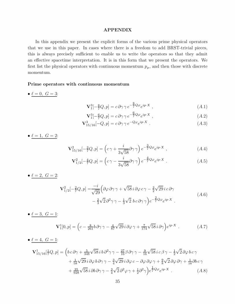
APPENDIX

In this appendix we present the explicit forms of the various prime physical operators

that we use in this paper. In cases where there is a freedom to add BRST-trivial pieces,

this is always precisely sufficient to enable us to write the operators so that they admit

an effective spacetime interpretation. It is in this form that we present the operators. We

first list the physical operators with continuous momentum pµ, and then those with discrete

momentum.

Prime operators with continuous momentum

• ℓ = 0, G = 3:

V31[−8

7Q, p] = c ∂γ γ e−87Qϕeip·X , (A.1)

V31[−6

7Q, p] = c ∂γ γ e−

67Qϕeip·X , (A.2)

V315/16[−Q, p] = c ∂γ γ e−Qϕeip·X . (A.3)

• ℓ = 1, G = 2:

V215/16[−3

7Q, p] =(c γ +

i

3√

58∂γ γ

)e−

37Qϕeip·X , (A.4)

V21/2[−4

7Q, p] =(c γ − i

3√

58∂γ γ

)e−

47Qϕeip·X . (A.5)

• ℓ = 2, G = 2:

V21/2[−2

7Q, p] =

−i√29

(∂ϕ ∂γ γ +

√58 i ∂ϕ c γ − 3

2

√29 i c ∂γ

− 23

√2 ∂2γ γ − 1

3

√2 b c ∂γ γ

)e−

27Qϕeip·X .

(A.6)

• ℓ = 3, G = 1:

V11[0, p] =

(c − 8

261b ∂γ γ − 487

√29 i ∂ϕ γ + 7

174

√58 i ∂γ

)eip·X . (A.7)

• ℓ = 4, G = 1:

V115/16[

17Q, p] =

(b c ∂γ + 5

348

√58 i b ∂2γ γ − 27

16β ∂γ γ − 916

√58 i c β γ − 1

2

√2 ∂ϕ b c γ

+ 158

√29 i ∂ϕ b ∂γ γ − 3

4

√29 i ∂ϕ c − ∂ϕ ∂ϕ γ + 9

8

√2 ∂ϕ ∂γ + 1

16∂b c γ

+ 35928

√58 i ∂b ∂γ γ − 3

4

√2 ∂2ϕ γ + 1

2∂2γ

)e

17

Qϕeip·X . (A.8)

35

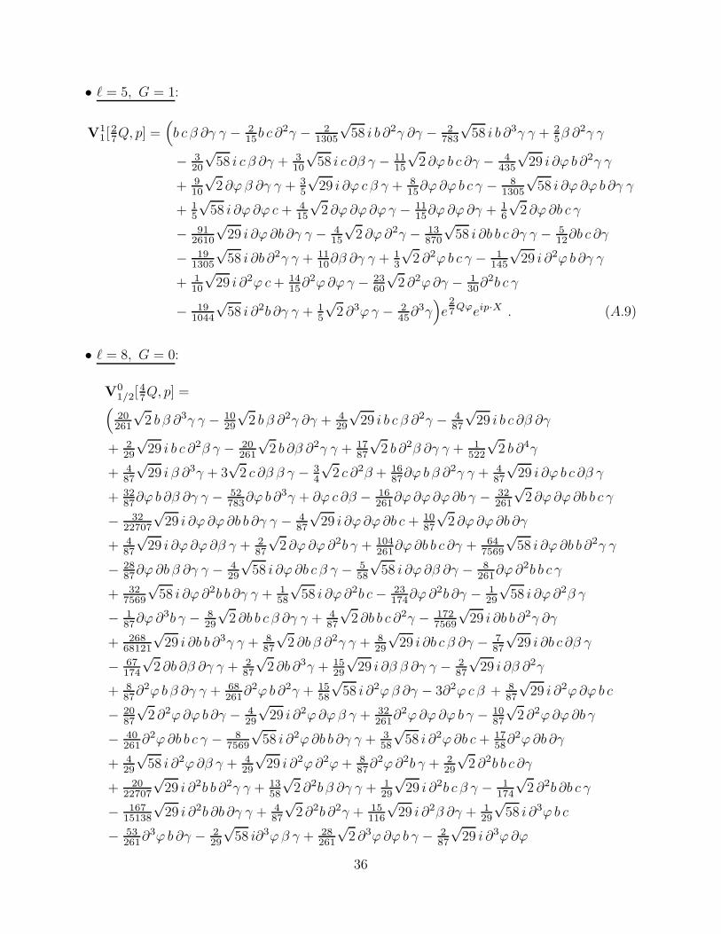
• ℓ = 5, G = 1:

V11[

27Q, p] =

(b c β ∂γ γ − 2

15b c ∂2γ − 21305

√58 i b ∂2γ ∂γ − 2

783

√58 i b ∂3γ γ + 2

5β ∂2γ γ

− 320

√58 i c β ∂γ + 3

10

√58 i c ∂β γ − 11

15

√2 ∂ϕ b c ∂γ − 4

435

√29 i ∂ϕ b ∂2γ γ

+ 910

√2 ∂ϕ β ∂γ γ + 3

5

√29 i ∂ϕ c β γ + 8

15∂ϕ ∂ϕ b c γ − 81305

√58 i ∂ϕ ∂ϕ b ∂γ γ

+ 15

√58 i ∂ϕ ∂ϕ c + 4

15

√2 ∂ϕ ∂ϕ ∂ϕ γ − 11

15∂ϕ ∂ϕ ∂γ + 16

√2 ∂ϕ ∂b c γ

− 912610

√29 i ∂ϕ ∂b ∂γ γ − 4

15

√2 ∂ϕ ∂2γ − 13

870

√58 i ∂b b c ∂γ γ − 5

12∂b c ∂γ

− 191305

√58 i ∂b ∂2γ γ + 11

10∂β ∂γ γ + 13

√2 ∂2ϕ b c γ − 1

145

√29 i ∂2ϕ b ∂γ γ

+ 110

√29 i ∂2ϕ c + 14

15∂2ϕ ∂ϕ γ − 2360

√2 ∂2ϕ ∂γ − 1

30∂2b c γ

− 191044

√58 i ∂2b ∂γ γ + 1

5

√2 ∂3ϕ γ − 2

45∂3γ

)e

27

Qϕeip·X . (A.9)

• ℓ = 8, G = 0:

V01/2[

47Q, p] =

(20261

√2 b β ∂3γ γ − 10

29

√2 b β ∂2γ ∂γ + 4

29

√29 i b c β ∂2γ − 4

87

√29 i b c ∂β ∂γ

+ 229

√29 i b c ∂2β γ − 20

261

√2 b ∂β ∂2γ γ + 17

87

√2 b ∂2β ∂γ γ + 1

522

√2 b ∂4γ

+ 487

√29 i β ∂3γ + 3

√2 c ∂β β γ − 3

4

√2 c ∂2β + 16

87∂ϕ b β ∂2γ γ + 4

87

√29 i ∂ϕ b c ∂β γ

+ 3287

∂ϕ b ∂β ∂γ γ − 52783

∂ϕ b ∂3γ + ∂ϕ c ∂β − 16261

∂ϕ ∂ϕ ∂ϕ ∂b γ − 32261

√2 ∂ϕ ∂ϕ ∂b b c γ

− 3222707

√29 i ∂ϕ ∂ϕ ∂b b ∂γ γ − 4

87

√29 i ∂ϕ ∂ϕ ∂b c + 10

87

√2 ∂ϕ ∂ϕ ∂b ∂γ

+ 487

√29 i ∂ϕ ∂ϕ ∂β γ + 2

87

√2 ∂ϕ ∂ϕ ∂2b γ + 104

261∂ϕ ∂b b c ∂γ + 64

7569

√58 i ∂ϕ ∂b b ∂2γ γ

− 2887∂ϕ ∂b β ∂γ γ − 4

29

√58 i ∂ϕ ∂b c β γ − 5

58

√58 i ∂ϕ ∂β ∂γ − 8

261∂ϕ ∂2b b c γ

+ 327569

√58 i ∂ϕ ∂2b b ∂γ γ + 1

58

√58 i ∂ϕ ∂2b c − 23

174∂ϕ ∂2b ∂γ − 129

√58 i ∂ϕ ∂2β γ

− 187∂ϕ ∂3b γ − 8

29

√2 ∂b b c β ∂γ γ + 4

87

√2 ∂b b c ∂2γ − 172

7569

√29 i ∂b b ∂2γ ∂γ

+ 26868121

√29 i ∂b b ∂3γ γ + 8

87

√2 ∂b β ∂2γ γ + 8

29

√29 i ∂b c β ∂γ − 7

87

√29 i ∂b c ∂β γ

− 67174

√2 ∂b ∂β ∂γ γ + 2

87

√2 ∂b ∂3γ + 15

29

√29 i ∂β β ∂γ γ − 2

87

√29 i ∂β ∂2γ

+ 887

∂2ϕ b β ∂γ γ + 68261

∂2ϕ b ∂2γ + 1558

√58 i ∂2ϕ β ∂γ − 3∂2ϕ c β + 8

87

√29 i ∂2ϕ ∂ϕ b c

− 2087

√2 ∂2ϕ ∂ϕ b ∂γ − 4

29

√29 i ∂2ϕ ∂ϕ β γ + 32

261∂2ϕ ∂ϕ ∂ϕ b γ − 10

87

√2 ∂2ϕ ∂ϕ ∂b γ

− 40261

∂2ϕ ∂b b c γ − 87569

√58 i ∂2ϕ ∂b b ∂γ γ + 3

58

√58 i ∂2ϕ ∂b c + 17

58∂2ϕ ∂b ∂γ

+ 429

√58 i ∂2ϕ ∂β γ + 4

29

√29 i ∂2ϕ ∂2ϕ + 8

87∂2ϕ ∂2b γ + 229

√2 ∂2b b c ∂γ

+ 2022707

√29 i ∂2b b ∂2γ γ + 13

58

√2 ∂2b β ∂γ γ + 1

29

√29 i ∂2b c β γ − 1

174

√2 ∂2b ∂b c γ

− 16715138

√29 i ∂2b ∂b ∂γ γ + 4

87

√2 ∂2b ∂2γ + 15

116

√29 i ∂2β ∂γ + 1

29

√58 i ∂3ϕ b c

− 53261∂3ϕ b ∂γ − 2

29

√58 i∂3ϕ β γ + 28

261

√2 ∂3ϕ ∂ϕ b γ − 2

87

√29 i ∂3ϕ ∂ϕ

36

− 14261

∂3ϕ ∂b γ + 7783

√2 ∂3b b c γ + 331

68121

√29 i ∂3b b ∂γ γ − 1

1044

√29 i ∂3b c

+ 23696

√2 ∂3b ∂γ + 8

261∂4ϕ b γ + 1

87

√58 i ∂4ϕ + 1

522

√2 ∂4b γ

)e

47

Qeip·X . (A.10)

Prime operators with discrete momentum

• ℓ = 1, G = 2:

D2[−67Q] =

(c γ − i

3√

58∂γ γ

)e−

67Qϕ , (A.11)

D2[−87Q] =

(c γ +

i

3√

58∂γ γ

)e−

87

Qϕ . (A.12)

• ℓ = 4, G = 0:

D0[0] = 1 . (A.13)

• ℓ = 6, G = 0:

D0[27Q] =(b β ∂γ γ − 3

5

√58 i b c β γ − 14

15b ∂2γ − 2120

√58 i β ∂γ + 261

10 c β

− 65

√29 i ∂ϕ b c − 11

15

√2 ∂ϕ b ∂γ − 6

5

√29 i ∂ϕ β γ − 4

5

√58 i ∂ϕ ∂ϕ + 8

15∂ϕ ∂ϕ b γ

+ 115

√2 ∂ϕ ∂b γ − 1

5∂b b c γ + 7

290

√58 i ∂b b ∂γ γ − 9

20

√58 i ∂b c − 97

60∂b ∂γ

− 65

√58 i ∂β γ − 8

5

√29 i ∂2ϕ + 8

15

√2 ∂2ϕ b γ − 8

15∂2b γ

)e

27

Qϕ .

(A.14)

37

REFERENCES

[1] A.B. Zamolodchikov, Teor. Mat. Fiz. 65 (1985) 1205.

[2] A. Bilal and J.-L. Gervais, Nucl. Phys. B314 (1989) 646.

[3] S.R. Das, A. Dhar and S.K. Rama, Mod. Phys. Lett. A6 (1991) 3055; Int. J. Mod. Phys.

A7 (1992) 2295.

[4] C.N. Pope, L.J. Romans and K.S. Stelle, Phys. Lett. B268 (1991) 167; Phys. Lett. B269

(1991) 287.

[5] C.N. Pope, L.J. Romans, E. Sezgin and K.S. Stelle, Phys. Lett. B274 (1992) 298.

[6] H. Lu, C.N. Pope, S. Schrans and K.W. Xu, Nucl. Phys. B385 (1992) 99.

[7] H. Lu, C.N. Pope, S. Schrans and X.J. Wang, Nucl. Phys. B379 (1992) 47.

[8] H. Lu, B.E.W. Nilsson, C.N. Pope, K.S. Stelle and P.C. West, “The low-level spectrumof the W3 string,” preprint CTP TAMU-64/92, hep-th/9212017.

[9] C.N. Pope, E. Sezgin, K.S. Stelle and X.J. Wang, “Discrete states in the W3 string,”preprint, CTP TAMU-64/92, hep-th/9209111, to appear in Phys. Lett. B.

[10] P.C. West, “On the spectrum, no ghost theorem and modular invariance of W3 strings,”preprint KCL-TH-92-7, hep-th/9212016.

[11] H. Lu, C.N. Pope, S. Schrans and X.J. Wang, “The interacting W3 string,” preprintCTP TAMU-86/92, KUL-TF-92/43, hep-th/9212117.

[12] C.N. Pope and X.J. Wang, “The ground ring of the W3 string,” preprint CTP-TAMU-3/93, to appear in the proceedings of the Summer School in High-Energy Physics andCosmology, Trieste 1992.

[13] S.K. Rama, Mod. Phys. Lett. A6 (1991) 3531.

[14] B.H. Lian and G.J. Zuckermann, Phys. Lett. B254 (1991) 541.

[15] E. Witten, Nucl. Phys. B373 (1992) 187;E. Witten and B. Zwiebach, Nucl. Phys. B377 (1992) 55.

[16] J. Thierry-Mieg, Phys. Lett. B197 (1987) 368.

[17] L.J. Romans, Nucl. Phys. B352 (1991) 829.

[18] K.S. Stelle, “W3 strings,” in proceedings of the Lepton-Photon/HEP Conference, Geneve1991 (World Scientific, Singapore, 1992).

[19] M.E. Peskin, “Introduction to string and superstring theory II,” lectures at the 1986Theoretical Advanced Study Institute in Particle Physics, Santa Cruz.

[20] A.A. Belavin, A.M. Polyakov and A.B. Zamolodchikov, Nucl. Phys. B241 (1984) 333.

[21] M.D. Freeman and P.C. West, “W3 string scattering,” preprint, KCL-TH-92-4, hep-th/9210134.

[22] K. Thielemans, Int. J. Mod. Phys. C2 (1991) 787.

[23] M.D. Freeman and P.C. West, “The covariant scattering and cohomology of W3 strings,”preprint, KCL-TH-93-2, hep-th/9302114.

38