On the recovery of multiple flow parameters from transient head data

Journal of Computational and Applied Mathematics 169 (2004) 1–15www.elsevier.com/locate/cam

On the recovery of multiple %ow parameters from transienthead data

Ian Knowlesa ;∗, Tuan Leb, Aimin Yana ;1

aDepartment of Mathematics, University of Alabama at Birmingham, 452 Campbell Hall, 1530 3rd Avenue S,Birmingham, AL 35294-1170, USA

bDepartment of Mathematics, University of New Orleans, New Orleans, LA 70148, USA

Received 12 November 2002; received in revised form 5 October 2003

Abstract

The problem of estimating groundwater %ow parameters from head measurements and other ancillary datais fundamental to the process of modelling a groundwater system. We consider here a new method that allowsfor the simultaneous computation of multiple parameters as the unique minimum of a convex functional.c© 2003 Elsevier B.V. All rights reserved.

Keywords: Groundwater; Con9ned aquifer; Parameter estimation; Steepest descent

1. Introduction

We are concerned here with a new deterministic method for identifying the %ow parameters ingroundwater models. It is common to assume that groundwater %ow in a con9ned isotropic aquiferis described by the equation

∇ · [K(x)∇w(x; t)] = S(x)9w9t − R(x; t); (1.1)

in which w represents the piezometric head, K the hydraulic conductivity, R the recharge–discharge, S the speci9c storage, t ¿ 0 represents time, and x varies over some bounded region of three-dimensional space representing the physical aquifer; see, for example, [2, (3.3.17)]. Whenthe piezometric head w does not vary appreciably in the vertical dimension, the equation can be

∗ Corresponding author.E-mail address: [email protected] (I. Knowles).

1 Supported in part by US National Science Foundation Grants DMS-9805629 and DMS-0107492.

0377-0427/$ - see front matter c© 2003 Elsevier B.V. All rights reserved.doi:10.1016/j.cam.2003.10.013

mailto:[email protected]

2 I. Knowles et al. / Journal of Computational and Applied Mathematics 169 (2004) 1–15

depth-averaged to obtain a two-dimensional formulation; in this case K becomes the transmissivity,S the (dimensionless) storativity, and R represents a combination of an averaged recharge-dischargeand vertical leakage terms. We are interested in the problem of the simultaneous determination ofthe functions K , S, and R, from measured data on w(x; t) at various points of and over some timeinterval, together with values of K measured at some boundary locations. Much has already beenwritten on various aspects surrounding this topic. In particular, the problem of the determination ofK from steady state head data has been extensively (though apparently not de9nitively) studied, seefor example [3,6,7], as well as [4,25] and the references therein for detailed survey information; thedetermination of K from transient data is discussed in [5,9,10,24]. There has also been some workon the determination of S [18] and R [22]. We note that there seems to be little documented workin the literature on the simultaneous determination of K , S, and R.

In [12] a new method for parameter estimation for elliptic equations (of which the steady stateequation for groundwater %ow is but one example) was introduced. In this method, the parameterestimation is accomplished by the minimization of a new functional which (as is shown in [12])has the important property of being convex; 2 this gives the approach signi9cant advantages overother methods, notably those of output least-squares type, in that the functional has a unique globalminimum, with no possibility of the associated descent algorithms “getting stuck” in spurious localminima.

In this paper, we explore in detail some of the practical aspects of the descent algorithms associatedwith this approach. In particular, we show that the method is eMective in simultaneously estimatingmultiple coeNcients in these equations. This is important in groundwater modelling in that one cannotreasonably expect to eMectively model a groundwater system without obtaining, in an appropriatelyobjective manner, proper estimations, or measurements, of all of the coeNcient functions in thatsystem. In accomplishing this task, it is clear from a mathematical standpoint that steady state datais insuNcient for specifying multiple coeNcients. One is thus inevitably attracted to the greaterinformation present in time varying head data. This in turn leads us to a consideration of theparabolic equation (1.1); we show in Section 2 that time varying data can be transformed to datafor certain elliptic equations of the type discussed above, to which our descent methods may thenbe applied.

We note in passing that these methods are particularly eMective when the underlying distributedparameters are discontinuous, a situation that one must assume to be the case a priori in a practicalsituation. We show also that the method can be adapted to obtain approximations to a time-varyingrecharge–discharge function R(x; t); such estimates have proven particularly diNcult to computeheretofore [1, p. 152]. The method also allows one to insert certain additional a priori informa-tion about the parameters being estimated directly into the algorithms. The ability to perform suchinsertions is an important factor in the numerical performance of the descent algorithms becausethe underlying problem of parameter estimation is quite ill-posed (i.e. any error in the measureddata can lead to large errors in the estimated parameters), and a common, and natural, route tocircumventing the numerical instabilities caused by ill-posedness is to input appropriate additionalindependent information (cf. [19]).

2 To be more precise, the functional is convex under the typical conditions encountered in practice (see [12]).

I. Knowles et al. / Journal of Computational and Applied Mathematics 169 (2004) 1–15 3

2. Reformulating the time-dependent problem

By choosing new units for the time as necessary, one can assume that 06 t6 1. So, givenmeasured head data w(x; t), where w is considered to be a solution of Eq. (1.1), and measuredvalues for K(x) on the boundary of our physical region , we seek to compute the functions K ,S, and R, where for simplicity we temporarily assume that R does not depend on time, i.e. thatR = R(x).

We begin by transforming the solution data w(x; t) of the parabolic Eq. (1.1) to data u(x; �), where

u(x; �) =∫ 1

0w(x; t)e−�t dt (2.1)

and u(x; �) satis9es an associated elliptic equation,

− ∇ · [K(x)∇u(x; �)] + �S(x)u(x; �) = R∗(x); (2.2)

where

R∗(x) =e−� − 1

�R(x) + S(x)[w(x; 0) − w(x; 1)e−�]: (2.3)

For any 9xed �¿ 0 it is a relatively simple matter to compute values u(x; �) from the known valuesfor w(x; t). We arrive then at a new problem: given u(x; �) for x in and all �¿ 0 (and K on theboundary of ), determine the functions K , S, and R.

3. The optimization method

We now apply the variational method proposed in [12] to (2.2). As mentioned above, we assumethat u(x; �) is known as a solution of (2.2) for all x in the region, and all �¿ 0. For each �¿ 0and functions k, s, and r let v = uk;s; r;� be the unique solution of the boundary value problem

−∇ · (k(x)∇v(x; �)) + �s(x)v(x; �) = r∗(x);

v|9 = u|9: (3.1)

where

r∗(x) =e−� − 1

�r(x) + s(x)[w(x; 0) − w(x; 1)e−�]: (3.2)

Notice that, in this notation u=uK;S;R;�, where K , S, and R are the functions that we seek to recover.Consider now the functional G(k; s; r; �) given by

G(k; s; r; �) =∫

k(x)(|∇u|2 − |∇uk;s; r;�|2)

+�s(x)(u2 − u2k; s; r;�) − 2r∗(x)(u − uk;s; r;�) dx: (3.3)

This functional is a generalization of the functional used in [14] to eMect numerical diMerentiationof a function of one variable; as is explained in the remark following [13, Theorem 2.1], the preciseform arises from converting a constrained energy functional minimization to an unconstrained one


using Lagrange multipliers. It is also worth observing that the nonnegativity of this functional isequivalent to the validity of the Dirichlet principle for the associated positive self-adjoint ellipticdiMerential operator; so the recovery of these coeNcient functions via such functionals provides,roughly speaking, a kind of inverse Dirichlet principle for this situation.

The functional, H , that we actually minimize to recover the desired %ow coeNcients, is formedby choosing nmax unequal positive values of the � parameter, �1; �2; : : : ; �nmax , and then setting

H (k; s; r) =nmax∑i=1

G(k; s; r; �i): (3.4)

As we seek to determine three functions K , S, and R, it is natural to expect that one would needto use at least three of the functions u(x; �i) in this process. That this is indeed the case followsfrom the uniqueness theorem in [12], where it is noted that one needs in addition that a certainvector 9eld generated by the three solution functions generates no trapped orbits, a condition that iseasily checked in practice via computer graphics generated directly from the computed data functionsu(x; �i), 16 i6 nmax (see [15]). This condition is linked to the natural restriction on this inverseproblem arising from the fact that in regions of no %ow, one cannot expect to recover %ow parametersby using only %ow data. So, in the above we must always take nmax¿ 3. In fact, it is advantageousto use nmax�3; we discuss this aspect in more detail later. We also note for later use that the sameuniqueness theorem requires that K be known on the boundary of the groundwater region; furtherdiscussion on the use of prior information may be found in [8,9, Section 6].

For convenience, we list some of the properties of the functional G established in [12]. First, from[12, Theorem 2.1(i)]

G(k; s; r; �) =∫

k(x)|∇(u − uk;s; r;�)|2 + �s(x)(u − uk;s; r;�)2 dx: (3.5)

For k positive de9nite, s¿ 0, and �¿ 0, one can see that we have G(k; s; r; �)¿ 0 and we alsohave that G(k; s; r; �) = 0 if and only if u = uK;S;R;� = uk;s; r;�. By a similar calculation to that of [12]we also have that the 9rst variation (Gateaux diMerential) of G is given by

G′(k; s; r; �)[h1; h2; h3] =∫

(|∇u|2 − |∇uk;s; r;�|2)h1(x)

+[�(u2 − u2k; s; r;�) + 2(e−�w(x; 1) − w(x; 0))(u − uk;s; r;�)]h2(x)

−2e−� − 1

�(u − uk;s; r;�)h3(x) dx: (3.6)

In this notation, the values of G′ represent various directional derivatives for the functional G, withthe functions hi serving as the “directions” in which one might choose to vary k, s, or r; for example,if we set h2 = h3 = 0 then from Taylor’s theorem for functionals, for all � small enough

G(k + �h1; s; r; �) ≈ G(k; s; r; �) + �G′(k; s; r; �)[h1; 0; 0] (3.7)

and so a knowledge of G′(k; s; r; �)[h1; 0; 0] allows us to estimate the diMerence G(k + �h1; s; r; �) −G(k; s; r; �) when �¿ 0 is not too large. In particular, in direct analogy with the gradient of a


function of several variables, we may take the function adjacent to h1 in (3.6) to be the gradient ofG with respect to k, ∇kG, i.e.

∇kG(k; s; r; �) = |∇u|2 − |∇uk;s; r;�|2: (3.8)

Similarly

∇sG(k; s; r; �) = �(u2 − u2k; s; r;�) + 2(e−�w(x; 1) − w(x; 0))(u − uk;s; r;�); (3.9)

∇rG(k; s; r; �) = −2e−� − 1

�(u − uk;s; r;�): (3.10)

Exactly as in the multivariate case, these gradients allow us to use descent methods for our mini-mization; in particular, if we choose to set h2 = h3 = 0 and

h1 = −∇kG(k; s; r; �);

we have that

G(k + �h1; s; r; �) ¡G(k; s; r; �)

for �¿ 0 and not too large, and so we can (locally) minimize G in the direction of h1 = −∇kG(k;s; r; �) with one-dimensional search techniques. Later descent steps can minimize G in s and r aswell. While the actual gradients that we use presently are somewhat diMerent, the general idea is thesame.

Notice that G′(k; s; r; �) = 0 (i.e. G′(k; s; r; �)[h1; h2; h3] = 0 for all functions h1; h2; h3) if and onlyif

|∇u|2 − |∇uk;s; r;�|2 = 0;

�(u2 − u2k; s; r;�) + 2(e−�w(x; 1) − w(x; 0))(u − uk;s; r;�) = 0;

2e−� − 1

�(u − uk;s; r;�) = 0;

which, from the form of (3.3), is true if and only if G(k; s; r; �) = 0; we know already that this istrue if and only if u = uK;S;R;� = uk;s; r;� again.

We next observe that the functional H in (3.4) has very similar properties. In particular, essentiallythe same argument shows that H ¿ 0, and that H (k; s; r) = 0 if and only if u = uK;S;R;�i = uk;s; r;�i forall 16 i6 n, and the derivative H ′(k; s; r)=0 if and only if H (k; s; r)=0. By choosing nmax¿ 3 andassuming that the vector 9eld condition mentioned earlier holds, it now follows from the uniquenessresult [12, Theorem 3.5] that (K; S; R) is not only the unique global minimum for H , but also theunique stationary point (one can also show from the second variation for H that under the sameconditions H is actually a convex functional, but we omit the details). This is the ideal contextfor numerical minimization and suggests a natural path to the goal of simultaneously computing thefunctions K , S, and R.

4. Time dependent recharge–discharge

It is not clear (and possibly not true) that the measured data in this problem uniquely determinesa fully time-dependent source term R(x; t). However, if we assume that R is piecewise constant in


time, then we can adapt the above procedure to recover such an R. In this case, if we assume that0 = t0 ¡t1 ¡ · · ·¡tm = 1 are 9xed times in our given time period, our R then takes the form

R(x; t) =n∑

i=1

Ri(x)�[ti−1 ;ti](t); (4.1)

where for each i,

�[ti−1 ;ti](t) =

{1 if ti−16 t6 ti;

0 otherwise:

This assumption on R in eMect assumes that, over the times 06 t6 t1, R is “frozen” as the functionR1(x) of the space variables, and over t16 t6 t2 R is R2(x), etc; each function Ri is thus a snapshotof R(x; t) over a part of the time measurement period. If the time sub-intervals are chosen suNcientlysmall, this allows us (in theory at least) to approximate the fully time dependent R as closely as welike.

Our inverse problem may then be stated as follows: given measured head data w(x; t), where wis considered to be a solution of Eq. (1.1), and measured values for K(x) on the boundary of ourphysical region , we seek to compute the functions K , S, and Ri, 16 i6 n.

As in Section 2, we can reformulate to an elliptic equation. At this juncture it is advantageous toobserve that the procedure outlined above can be applied to each interval [ti−1; ti], 16 i6 n, as aseparate calculation. So we set

ui(x; �) =∫ ti

ti−1

w(x; t)e−�t dt (4.2)

and, analogous to (2.2), we obtain for each i, 16 i6 n,

− ∇ · [K(x)∇ui(x; �)] + �S(x)ui(x; �) = R∗i (x); (4.3)

where

R∗i (x) = −1

�Ri(x)[e−�ti−1 − e−�ti ] + S(x)[w(x; ti−1)e−�ti−1 − w(x; ti)e−�ti ]: (4.4)

So now, for each i, 16 i6 n, we are given ui(x; �) and we seek K , S, and Ri.The functional G in this case has the form given by (3.3) where now G = G(k; s; ri; �) and the

term r∗i (formerly de9ned by Eq. (3.2)) is given by

r∗i (x) = −1

�ri(x)[e−�ti−1 − e−�ti ] + s(x)[w(x; ti−1)e−�ti−1 − w(x; ti)e−�ti ] (4.5)

and the solutions uk;s; r;� are written uk;s; ri ;�. The gradients ∇kG and ∇sG are given, as before, by(3.8) and (3.9); in place of ∇rG, we have ∇riG, 16 i6 n, where

∇riG(k; s; ri; �) = −2e−�ti−1 − e−�ti

�(u − uk;s; ri ;�): (4.6)

In this case, the functional H is again given by Eq. (3.4) with nmax¿ 3, and the relevant unique-ness properties giving conditions on the appropriate vector 9eld under which this H has a uniqueminimum (and a unique stationary point) at (K; S; Ri) are the same as above.

In the next section, we discuss the descent process in greater detail.


5. A descent algorithm

We now consider some of the details of our minimization procedure. The gradients de9ned by(3.8)–(3.10) are commonly termed L2-gradients because one can write (for example)

G′(k; s; r; �)[h1; 0; 0] = (∇kG; h1)L2 ;

where (·; ·)L2 denotes the standard inner product in the Hilbert space of square integrable functions,L2(). In order keep the value of K on the boundary 9xed throughout the descent process, wehave found it advantageous to use a class of gradients introduced in [17]. These Neuberger gradientsare a type of preconditioned (i.e. smoothed) gradient that generally give superior convergence insteepest descent algorithms. We shall use the notation ∇N

k G to denote the Neuberger smoothing of∇kG, de9ned by

G′(k; s; r; �)[h1; 0; 0] = (∇Nk G; h1)H1 ; (5.1)

where the above identity is to hold for all choices of h1 belonging to the Sobolev space H1()consisting of all functions in L2() whose derivatives also lie in L2(), and (·; ·)H1 denotes theinner product of functions in this Sobolev space. The Neuberger gradients ∇N

s G and ∇Nr G (or ∇N

ri G,16 i6 n) are de9ned analogously. In order to compute the Neuberger gradient ∇N

k G (for example)we merely have to solve the boundary value problem

− �g + g = ∇kG; (5.2)

g|9 = 0 (5.3)

and note from [12, Eq (3.1)] that g = ∇Nk G; notice here that, as g|9 = 0, the boundary data for K

is preserved during the descent process. The Neuberger gradients ∇Ns G and ∇N

r G are computed inan analogous manner.

In implementing the descent procedure when R = R(x), for example, one could choose to descendby varying all of k; s; r at each descent step. However, we have found that this strategy is notparticularly eNcient because the rate at which H decreases with respect to k is substantially smallerthan that for s and r. So our general strategy is to proceed in cycles of three, with a greaternumber of descent steps allocated to descent with respect to k compared to descent with respectto s or r. For a given choice of the initial functions, k0; s0; r0, one could use steepest descent,beginning with the direction −∇N

k H (k0; s0; r0), together with a one-dimensional search routine, toline minimize H at some point (k1; s0; r0), where k1 is the latest approximation to the function K(this step would normally be repeated a predetermined number of times); this would be followedwith a line minimization in the direction −∇N

s H (k1; s0; r0) to obtain functions (k1; s1; r0), and thenby another line minimization in the direction −∇N

r H (k1; s1; r0) to obtain functions (k1; s1; r1); thisthree step cycle would be repeated until convergence.

In practice one gets faster (by, roughly, a factor of two) convergence with the following adaptionof the standard Polak–RibiSere conjugate gradient scheme [20, p. 304]. The initial search directionis h0 = g0 = −∇N

k H (k0; s0; r0). At (ki; si; ri) one uses the approximate line search routine to mini-mize H (k; s; r) in the direction of hi, resulting in (ki+1; si; ri). Then gi+1 = −∇N

k H (ki+1; si; ri), and


hi+1 = gi+1 + �ihi, where

�i =(gi+1 − gi; gi+1)H1

(gi; gi)H1=

(gi+1 − gi;∇kH (ki; si; ri))L2

(gi;∇kH (ki; si; ri))L2:

At (ki+1; si; ri), one uses ∇sH (ki+1; si; ri) in the same way to determine (ki+1; si+1; ri), and then∇rH (ki+1; si+1; ri) to obtain (ki+1; si+1; ri+1), whereupon the three-step cycle repeats.

When the recharge–discharge term is time dependent (according to the discussion in Section 4)we use the same process. We discuss some of the practical issues (like how large may one choosen) in the next section.

6. Implementation and results

We describe here some of our tests involving various choices of synthetically produced data, andlater we consider some partial results from well data obtained over a period of about eight monthsat seven monitoring wells situated in the vicinity of the campus of the University of Alabama atBirmingham.

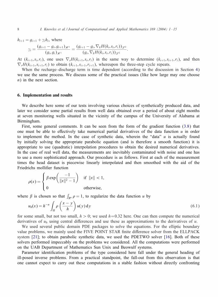
First, some general comments. It can be seen from the form of the gradient function (3.8) thatone must be able to eMectively take numerical partial derivatives of the data function u in orderto implement the method. In the case of synthetic data, wherein the “data” u is actually foundby initially solving the appropriate parabolic equation (and is therefore a smooth function) it isappropriate to use (quadratic) interpolation procedures to obtain the desired numerical derivatives.In the case of real well data, the measurements are inevitably contaminated with noise and one hasto use a more sophisticated approach. Our procedure is as follows. First at each of the measurementtimes the head dataset is piecewise linearly interpolated and then smoothed with the aid of theFriedrichs molli9er function

�(x) =

� exp( −1

‖x‖2 − 1

)if ‖x‖¡ 1;

0 otherwise;

where � is chosen so that∫Rn � = 1, to regularize the data function u by

uh(x) = h−n∫

�

(x − y

h

)u(y) dy (6.1)

for some small, but not too small, h¿ 0; we used h=0:32 here. One can then compute the numericalderivatives of uh using central diMerences and use these as approximations to the derivatives of u.

We used several public domain PDE packages to solve the equations. For the elliptic boundaryvalue problems, we mainly used the FIVE POINT STAR 9nite diMerence solver from the ELLPACKsystem [21]; to obtain parabolic synthetic data, we used the PDETWO solver [16]. Both of thesesolvers performed impeccably on the problems we considered. All the computations were performedon the UAB Department of Mathematics Sun Unix and Beowulf systems.

Parameter identi9cation problems of the type considered here fall under the general heading ofill-posed inverse problems. From a practical standpoint, the fall-out from this observation is thatone cannot expect to carry out these computations in a stable fashion without directly confronting


this issue. Many general methods for dealing with ill-posedness have been proposed, includingTikhonov regularization [23], limiting the number of grid points (ill-posedness tends to become morepronounced as the grids become 9ner), and limiting the number of iterations in iterative estimationprocedures, and even casting out the direct approach in favour of a statistically based approach [11].In the groundwater problem, there are diNculties associated with each of these choices: all Tikhonovregularization methods make use of a regularization parameter whose critical value must be knownquite accurately for the method to be eMective, and this can be problematical in the case of sparse,noisy aquifer data; if one limits the grid size too severely, the model error may increase unacceptably;if one limits the number of iterations, one may not be able to extract all of the information in thedata.

In the case of the present algorithm, we observed in our early trials that the main symptom ofill-posedness in the computations was a tendency of the computed values for the hydraulic conduc-tivity, K , to slowly become unbounded below. As the elliptic solvers are quite sensitive to a lossof positive de9niteness for K , the program would crash quite quickly when negative values of Kwere encountered. Now with 9eld data, one generally can input a reasonable estimate for a positivelower bound, c¿ 0, for the conductivity. We then modi9ed the program so that at each descentstep the values for ki smaller than c were set equal to c (and similar cutoMs were incorporated intothe computations of the other coeNcients, whenever justi9able on physical grounds). The eMect wasquite dramatic: the algorithm became extremely stable, and we were able to let it run over hundredsof thousands of descent steps without serious degradation of the resulting images. In particular, itnow became possible to simultaneously recover multiple coeNcients, albeit at the cost of an increas-ing amount of computer time as the number of coeNcients increased. It should be noted that in atypical least-squares minimization it is common to see large oscillations in the parameter values withunboundedness both from above and below. It appears that in our case, if one is to extrapolate fromthe computations exhibited here, the combination of an enforced lower bound and the convexity ofthe functional essentially eliminates the tendency for the parameter values to become unboundedabove.

We also found that increasing the value of nmax in the de9ning equation for H (Eq. (3.4))substantially improved the images; this is in line with the observation that ill-posedness is in somesense a manifestation of information loss, and so it makes sense that one should always strive toadd information whenever possible. In the results below we typically used nmax = 20, and we chosethe �j so that 0 ¡�j6 1. As � is the transformed time parameter, it is not unreasonable to expectthat using an even greater value of nmax would correspond to increasing the time resolution in theparabolic equation and should give even better results. In general, the method is %exible enough toallow the inclusion of multiple datasets, so that one may further decrease the natural ill-posednessassociated with groundwater data. Mathematically, as we are minimizing a convex functional theonly manifestation of ill-posedness is the “%atness” of H in a neighbourhood of the unique globalminimum, and one would expect less %atness in the presence of additional data.

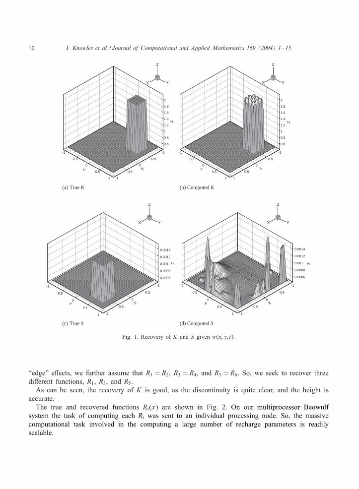
In Figs. 1 and 2, we demonstrate the simultaneous recovery of eight coeNcient functions fromknown data on the solution w(x; t), where x takes values in a two-dimensional region. We deliberatelychose discontinuous K , S, and R = R(x; t) for this test, both because the recovery of discontinuousfunctions is more diNcult than the recovery of smooth ones, and because in the 9eld, subsurfaceparameters are unlikely to be smooth functions. We assume that R has the form (4.1) where thetime interval 06 t6 1 is divided into six equal sub-intervals (so, n = 6). In order to investigate


0.6

0.8

1

1.2

1.4

1.6

1.8

2

Z

-1

-0.5

0

0.5

1

X

-1

-0.5

0

0.5

1

Y

X Y

Z

X Y

Z

X Y

Z

X Y

Z

(a) True K

0.6

0.8

1

1.2

1.4

1.6

1.8

2

Z

-1

-0.5

0

0.5

1

X

-1

-0.5

0

0.5

1

Y

0.0006

0.0008

0.001

0.0012

0.0014

Z

-1

-0.5

0

0.5

1

X

-1

-0.5

0

0.5

1

Y

(c) True S

0.0006

0.0008

0.001

0.0012

0.0014

Z

-1

-0.5

0

0.5

1

X

-1

-0.5

0

0.5

1

Y

(d) Computed S

(b) Computed K

Fig. 1. Recovery of K and S given w(x; y; t).

“edge” eMects, we further assume that R1 = R2, R3 = R4, and R5 = R6. So, we seek to recover threediMerent functions, R1, R3, and R5.

As can be seen, the recovery of K is good, as the discontinuity is quite clear, and the height isaccurate.

The true and recovered functions Ri(x) are shown in Fig. 2. On our multiprocessor Beowulfsystem the task of computing each Ri was sent to an individual processing node. So, the massivecomputational task involved in the computing a large number of recharge parameters is readilyscalable.


(a) True R1,R2 (b) Computed R1 (c) computed R2

(d) True R3,R4 (e) Computed R3 (f) Computed R4

(g) True R5,R6 (h) Computed R5 (i) Computed R6

Fig. 2. Recovery of R(x; y; t) given w(x; y; t).

The computed S is more of a problem. The main diNculty here appears to be that small errorsin the computed K , and, to a lesser extent, R seem to have noticable eMects on the recovery of S,because we have recovered this true S quite well when K and R are assumed known, and only S isbeing recovered, as may be seen in Fig. 3. On the other hand, it is worth noting that even though the


Fig. 3. Recovery of S given K .

Time (t)

Err

or

(%)

0 0.25 0.5 0.75 10

0.1

0.2

0.3

0.4

0.5

0.6

0.7

0.8

0.9

Fig. 4. Model error.

S recovery does not appear as eMective as the others, the model seems to be relatively insensitive tothis error, probably because the values of S are so small in the 9rst place. The model error is shownbelow in Fig. 4. Here we have graphed the maximum relative error between the model values andthe “true” head data, over the space grid points as a function of time. This shows that the modelformed from the above K , S, and R well approximates the original problem.

The data for Figs. 1 and 2 was obtained by using the PDE package PDETWO [16] to solve the2-d parabolic equation (1.1) over a square region

{(x; y) : −16 x6 1;−16y6 1}and with 06 t6 1; the chosen time step was h = 10−7 and we used a 30 × 30 grid on the spatialdomain. We used the initial condition

w(x; y; 0) = 2 + 0:5 cos !x cos !y

(to simulate slowly varying head data), and boundary conditions

w(x;−1; t) = 2 − (0:5 − t) cos !x;

w(x; 1; t) = 2 − (0:5 − t) cos !x;


Time (t)

Err

or

(%)

0 0.25 0.5 0.75 1

12

13

14

15

16

17

18

19

20

21

22

Fig. 5. Sparse data test.

w(−1; y; t) = 2 − (0:5 − t) cos !y;

w(1; y; t) = 2 − (0:5 − t) cos !y:

This parabolic data was then transformed to elliptic data u(x; y; �) via formula (2.1) and a Simpson’srule quadrature.

A valid criticism of the tests done thus far is that practical head data is both sparse and noisy, sothat in particular one does not have head data at every point on a 30×30 grid as we assumed above.In the next test, we 9rst computed w(x; t) at discrete times on the same 30×30 grid for given K , S,and R(x) as above, where we now consider these values as our “true” head data at each discrete time.Then we discarded 99% of the interior head values, keeping a regular grid containing nine interiorvalues, and on the boundary we kept the corresponding boundary data points to complete the regulargrid. To the surviving head values we added 20% relative error and then piecewise two-dimensionallinearly interpolated these data values to obtain our synthetic “measured” head dataset. From this datathe K , S, and R were recovered as above, and used to produce the model head values. The maximumrelative error over the space grid points as a function of time, between these model values and the“true” head data is graphed in Fig. 5 above. As can be seen, the maximum error is comparable tothe added noise. This and other similar trials indicate that the recovery process appears to be stablewith respect to sparse well sites and head measurement error.

We also investigated the practical utility of the method by means of measurements of %ow datagathered from seven wells located on the UAB campus over a period of about 8 months, andassuming a con9ned depth-averaged two-dimensional model for the aquifer. The results are shownin Fig. 6. The data was 9rst interpolated piecewise linearly on the irregular triangular grid formedin a rectangle containing the measurement points, and then smoothed and diMerentiated by using thetechnique outlined in [13, Section 5]. Each side of the rectangle contained one measurement point,and at each of these boundary points we also measured the value of K (in units of feet/minute)using a standard bail test in which the head is measured in the pumping well [15, p. 58]; here thestorativity S is dimensionless and R has units of feet/minute. We ran the computation 9rst under the


10.5

0.4

0.8

5

y0

-0.5

z1.2

1.6

x0

-0.5-1

10.5

(a) K

1

–0.015

0

0.55

y0

-0.5

z 0

0.015

0.0030 003

x0

-0.5-1

10.5

(b) S

10.5

0

5

y0

-0.5

z

20

40

x0

-0.5-1

10.5

(c) R = R(x;y)

Fig. 6. UAB data.

assumption that R=R(x), and later assumed that R had the form (4.1) with n=2; 3. In each case thecomputed values for K and S were essentially the same, with the computed functions Ri(x) showingsome modest variation. It is found in practice that values for S typically lie in the range 0.00005–0.005. The computed values of S are approximately consistent (see, for example, [1, p. 41]) withthe sand and clay mixture that is known to constitute much of the subsurface region under UAB[15, p. 56].

The irregular appearance of K on the boundary can be traced to the fact that we had only onemeasured value for K on each side of our rectangular region, because we were unable to carryout the transmissivity measurement at three of our seven wells. We have observed from our testson synthetic data that in such cases, while the values of K near the boundary were in general notreliable, interior values of K were usually quite good (see for example [14, Fig. 3]). In all cases theminimizations were very stable, and “ran out of steam” after about 150 iterations, which indicatesthat the parameters shown in Fig. 6 are plausible candidates for the “best 9t” for this dataset. As ourdata did not come with any solute information, we were not able to complete the task of forming acomplete %ow/solute model at this point in time. We hope to remedy this in a future study. We notein passing that one can use similar techniques to recover not only the full hydraulic conductivitytensor, but also solute parameters like the porosity and the hydrodynamic dispersion tensor as wellvarious solute source terms.

In summary, these tests indicate that veri9ably reliable recovery of multiple subsurface parameters,which of course includes the solution of the full inverse groundwater problem discussed earlier, maynow be possible.


Finally, we take the opportunity here to thank the referees for their careful reading of the originalmanuscript; their suggestions led to substantial improvements in the 9nal version of the paper.

References

[1] M.P. Anderson, W.W. Woessner, Applied Groundwater Modeling, Academic Press, New York, 1992.[2] J. Bear, A. Verruijt, Modeling Groundwater Flow and Pollution, D. Reidel Publishing Co., Dordrecht, 1992.[3] H. Ben Ameur, G. Chavent, J. JaMrUe, Re9nement and coarsening indicators for adaptive parametrization: application

to the estimation of hydraulic transmissivities, Inverse Problems 18 (3) (2002) 775–794.[4] J. Carrera, State of the art of the inverse problem applied to the %ow and solute equations, in: E. Custodio (Ed.),

Groundwater Flow and Quality Modelling, Kluwer Academic, Dordrecht, 1988, pp. 549–583.[5] J. Carrera, S.P. Neuman, Estimation of aquifer parameters under transient and steady-state conditions: 2. Uniqueness,

stability and solution algorithms, Water Resour. Res. 22 (1986) 211–227.[6] G. Chavent, Identi9cation of distributed parameter systems: about the output least square method, its implementation

and identi9ability, in: R. Iserman (Ed.), Proceedings of the Fifth IFAC Symposium on Identi9cation and SystemParameter Estimation, Vol. 1, Pergamon Press, Oxford, 1980, pp. 85–97.

[7] G. Chavent, On the theory of practice of nonlinear least-squares, Parameter identi9cation in ground water %ow,transport, and related processes, Part I, Adv. Water Res. 14 (2) (1991) 55–63.

[8] Y. Emsellem, G. de Marsily, An automatic solution for the inverse problem, Water Resour. Res. 7 (5) (1971)1264–1283.

[9] T.R. Ginn, J.H. Cushman, M.H. Houch, A continuous-time inverse operator for groundwater and contaminanttransport modeling: deterministic case, Water Resour. Res. 26 (1990) 241–252.

[10] D.L. Hughson, A. Gutjahr, EMect of conditioning randomly heterogeneous transmissivity on temporal hydraulic headmeasurements in transient two-dimensional aquifer %ow, Stochastic Hydrol. Hydraul. 12 (1998) 155–170.

[11] A.G. Journel, J.C. Huijbregets, Mining Geostatistics, Academic Press, San Diego, CA, 1978.[12] I. Knowles, Uniqueness for an elliptic inverse problem, SIAM J. Appl. Math. 59 (4) (1999) 1356–1370, Available

online at http://www.math.uab.edu/knowles/pubs.html.[13] I. Knowles, Parameter identi9cation for elliptic problems, J. Comput. Appl. Math. 131 (2001) 175–194.[14] I. Knowles, R. Wallace, A variational solution of the aquifer transmissivity problem, Inverse Problems 12 (1996)

953–963.[15] T.A. Le, An inverse problem in groundwater modeling. Ph.D. Thesis, University of Alabama at Birmingham, 2000.[16] D. Melgaard, R.F. Sincovec, General software for two-dimensional nonlinear partial diMerential equations, ACM

Trans. Math. Software 7 (1) (1981) 106–125.[17] J.W. Neuberger, Sobolev Gradients in DiMerential Equations, in: Lecture Notes in Mathematics, Vol. 1670, Springer,

New York, 1997.[18] S.P. Neumann, Perspective on “delayed yield”, Water Resour. Res. 15 (1979) 899–908.[19] L.E. Payne, Improperly Posed Problems in Partial DiMerential Equations, SIAM, Philadelphia, 1975.[20] W.H. Press, B.P. Flannery, S.A. Teukolsky, W.T. Vetterling, Numerical Recipes: The Art of Scienti9c Computing,

Cambridge University Press, Cambridge, 1989.[21] J.R. Rice, R.F. Boisvert, Solving Elliptic Problems Using ELLPACK, Springer, Berlin, 1985.[22] J. Simmers, Estimation of Natural Groundwater Recharge, in: NATO ASI Series C, Vol. 222, D. Reidel Publishing

Co., Dordrecht, 1988.[23] A.N. Tikhonov, V.Y. Arsenin, Solutions of Ill-Posed Problems, V.H. Winston & Sons, Washington, DC, 1977.[24] G.R. VUazquez, M. Guidici, G. Parravicini, G. Ponzini, The diMerential system method for the identi9cation of

transmissivity and storativity, Trans. Porous Media 26 (1997) 339–371.[25] W.W.-G. Yeh, Review of parameter identi9cation procedures in groundwater hydrology: the inverse problem, Water

Resour. Res. 22 (2) (1986) 95–108.

http://www.math.uab.edu/knowles/pubs.html

On the recovery of multiple flow parameters from transient head data

Documents

Transcript of On the recovery of multiple flow parameters from transient head data