On the Mahler measure of resultants in small

dimensions

Carlos D’Andrea

Department d’Algebra i Geometrıa, Universitat de Barcelona, Gran Via de lesCorts Catalanes 585, 08007 Barcelona. Spain

Matilde N. Lalın

Mathematical Sciences Research Institute, 17 Gauss Way, Berkeley, CA 94720

Abstract

We prove that sparse resultants having Mahler measure equal to zero are thosewhose Newton polytope has dimension one. We then compute the Mahler measureof resultants in dimension two, and examples in dimension three and four. Finally, weshow that sparse resultants are tempered polynomials. This property suggests thattheir Mahler measure may lead to special values of L-functions and polylogarithms.

Key words: Sparse resultants, Mahler measure, height, Newton polytope,polylogarithms, tempered polynomials.

1 Introduction

Let A0, . . . ,An ⊂ Zn be finite sets of integral vectors, Ai := {aij}j=1,...,ki. We

denote with ResA0,...,An ∈ Z[X0, . . . , Xn] the associated mixed sparse resultant,which is an irreducible polynomial in n + 1 groups Xi := {xij; 1 ≤ j ≤ ki} ofki variables each. It has the following geometric interpretation: consider thesystem

Fi(t1, . . . , tn) :=ki∑

j=1

xijtaij = 0 i = 0, . . . , n (1)

Email addresses: carlos@dandrea.name (Carlos D’Andrea),mlalin@math.ubc.ca (Matilde N. Lalın).

Preprint submitted to Elsevier Science 16 April 2006

of Laurent polynomials in the variables t1, . . . , tn. Here ta stands for ta11 ta2

2 . . . tann

where a = (a1, . . . , an). The resultant ResA0,...,An vanishes on a particular spe-cialization of the xij in an algebraically closed field K if the specialized system(1) has a common solution in (K \ {0})n. See [CLO,Stu] for a precise definitionof ResA0,...,An and some basic facts.

Resultants are of fundamental importance for solving systems of polynomialequations and therefore have been extensively studied [CLO,DAn,EM,Khe,Min,Stu].Recent research has focused on arithmetic aspects of this polynomial such asits height and its Mahler measure [DH,KPS,Som2].

Recall that the absolute height of g :=∑

α cαXα ∈ C[X0, . . . , Xn] is defined asH(g) := max{|cα|, α ∈ Nk}, where k := k0 + . . . + kn. Its (logarithmic) heightis given by

h(g) := log H(g) = log max{|cα|, α ∈ Nk}.

The Mahler measure of g is defined as

m(g) :=1

(2πi)k

∫

Tk

log |g(X0, . . . , Xn)| dX0

X0

. . .dXn

Xn

,

where for i = 0, . . . , n, dXi

Xiis an abbreviation for

∏k0j=1

dxij

xij, and

Tk = {(z1, . . . , zk) ∈ Ck| |z1| = . . . = |zk| = 1}

is the k-torus.

Some general relationships between the height and the Mahler measure are es-tablished in [EW, Chapter 3] as well as [KPS,Som1]. In [Som2] upper boundsfor both the height and the Mahler measure of resultants are presented. How-ever, very little seems to be known about the problem of explicitly computingboth the height and the Mahler measure of resultants. In the case of heights,a first attempt was done in [DH], where the heights of resultants in low degreeand one variable are calculated.

Jensen’s formula gives a simple expression for the Mahler measure of a uni-variate polynomial as a function on its roots. However, it is in general a veryhard problem to give an explicit closed formula for the Mahler measure of amultivariate polynomial. The simplest examples are

2

Theorem 1.1 • [Smy1, Example 5]

m(1 + x + y) =3√

3

4πL(χ−3, 2) = L′(χ−3,−1), (2)

where

L(χ−3, s) :=∞∑

h=1

χ−3(h)

hswith χ−3(h) :=

1 if h ≡ 1 mod 3

−1 if h ≡ −1 mod 3

0 if h ≡ 0 mod 3

is the Dirichlet L-series in the odd character of conductor 3.• Smyth also proved (see [Boy, Appendix 1]):

m(1 + x + y + z) =7

2π2ζ(3), (3)

where ζ denotes the Riemann zeta function.

In this paper we focus in the explicit computation of the Mahler measureof ResA0,...,An in the case where the dimension of N(ResA0,...,An) (the New-ton polytope of ResA0,...,An) is small. We assume that the family of supportsA0, . . . ,An is essential (see [Stu, Sec.1]), so ResA0,...,An is a polynomial of pos-itive degree in the variables xij. It is well-known (see [EW, Lemma 3.7]) thatwe always have m(ResA0,...,An) ≥ 0. The reason we focus in the dimensionof the Newton polytope of the resultant and not in the number of variablesand/or the size of the supports is due to some properties of the Mahler mea-sure with respect to homogeneousness and changes of variables. For instance,the Mahler measure of a homogeneous polynomial is the same as the Mahlermeasure of the corresponding dehomogenized polynomial. Moreover,

Lemma 1.2 [Smy2, Lemma 7] Let P (y) be a p-variable polynomial, and letV be a non-singular p× p integer matrix, then

m(P (y)) = m(P (yV )),

where yV denotes (∏

j yv1j

j , . . . ,∏

j yvpj

j ) for y = (y1, . . . , yp) and V = {vij}.

The whole situation may be summarized as follows: computing the Mahlermeasure of a polynomial whose Newton polytope has dimension p is the sameas computing the Mahler measure of a p-variable polynomial. This is importantbecause we may expect different kinds of formulas according to the number ofvariables (meaning the dimension of the Newton polytope). For speculationsconcerning this matter, see [Lal].

3

Evidence for this situation is Theorem 1 in Section 2 which states that ResA0,...,An

has Mahler measure equal to zero if and only if its Newton polytope has di-mension one, i.e. it is a segment.

This result shows that Mahler measures and heights behave differently inresultants. For instance, if we set n = 1, A0 = {0, 1}, A1 = {0, 1, . . . , `}, thenit turns out that

ResA0,A1 = ±∑

j=0

(−1)jx1jx`−j00 xj

01,

and from here it is easy to see that h(ResA0,A1) = 0. On the other hand,

setting yj = (−1)jx1jx`−j00 xj

01,

m(ResA0,A1) = m

∑

j=0

yj

.

The change of variables is allowable, because the x1j are algebraically inde-pendent,so we may apply Lemma 1.2.

Dehomogeneizing, one obtains

m(ResA0,A1) = m(1 + s1 + s2 + . . . + s`),

and this has been shown to be equal to 12log(`+1)− γ

2+O

(log(`+1)

`+1

)as ` →∞,

where γ is the Euler–Mascheroni constant (see [Smy1], and also [R-VTV] formore estimates and generalizations).

Moreover, it is still unknown a characterization of all supports A0, . . . ,An

having h(ResA0,...,An) = 0.

In Section 2 we deal with sparse resultants having Mahler measure zero. Thenwe proceed to higher dimensions. In Section 3 we focus on the case where theNewton polytope of the resultant has dimension two or three. In Theorem 2, wecompute the Mahler measure of resultants in dimension two, and in Theorem 4,we show that computing the Mahler measure of resultants in dimension threeis essentially equivalent to the computation of Mahler measures of univariatetrinomials. In Theorem 6 we compute the Mahler measure of trinomials havingthe same support. In Section 4 we compute the Mahler measure of a non trivialexample in dimension four.

All the computations can be expressed in terms of linear combinations ofpolylogarithms evaluated at algebraic numbers. From the point of view of

4

Mahler measure, it is natural to wonder why we would expect resultants tobe a source of interesting examples of multivariate polynomials.

In [Den] Deninger established the relation between Mahler measure and reg-ulators (see also [RV,Lal2]). More specifically, the Mahler measure of an ir-reducible polynomial P ∈ Q[s1, . . . , sp] is interpreted in terms of a specialvalue of the regulator η(s1, . . . , sp) in X , the projective variety determinedby {P = 0}. The regulator on the symbol {s1, . . . , sp} ∈ KM

p (C(X )) ⊗ Q isinitially defined in the cohomology of X \ {poles and zeros of si}. A sufficientcondition for extending it to the cohomology of X is that the tame symbols ofthe facets are trivial. In that case the polynomial is called tempered ([RV]).

If the symbol {s1, . . . , sp} is trivial, then the tame symbols of the facets aretrivial and η(s1, . . . , sp) is exact, and easily integrable by means of StokesTheorem. This is the first step that may lead to a Mahler measure involvingspecial values of polylogarithms ([Lal2]).

While the symbol is not necessarily trivial for a general polynomial, it is trivialfor the case of sparse resultants. This is the content of Section 5. In Theorem8, we show that resultants have trivial symbol, and so they are temperedpolynomials. This fact suggests that the Mahler measure of resultants maybe expressible in terms of combinations of polylogarithms and that we mightexpect results in the style of the ones from Sections 3 and 4 to be held in moregenerality.

2 Resultants with Mahler measure equal to zero

The the main result of this section is the following:

Theorem 1 m(ResA0,...,An) = 0 ⇐⇒ dim(N(ResA0,...,An)) = 1.

PROOF. Assume first that dim(N(ResA0,...,An)) = 1. We use Proposition4.1 in [Stu], which characterizes all families of essential supports A0, . . . ,An

such that the dimension of the Newton polytope is one: they must satisfyki := 2, i = 0, . . . , n. It turns out that ([Stu, Proposition 1.1]) in this caseResA0,...,An must be of the form ±(Xλ1−Xλ2), with λ1, λ2 ∈ Nk. It is very easyto see that polynomials of this kind have Mahler measure zero because theyare a monomial times the evaluation of T − 1 in another Laurent monomial.

For the converse, assume that m(ResA0,...,An) = 0,. Recall that the resul-tant is a primitive polynomial in Z[X0, . . . , Xn]. By Kronecker’s Lemma (see

5

for instance [EW, Theorem 3.10]), ResA0,...,An must be a monomial times aproduct of cyclotomic polynomials evaluated in monomials. But ResA0,...,An isirreducible in C[X0, . . . , Xn] as it is the equation of an irreducible surface inthe projective complex space (see [Stu, Lemma 1.1]). Having its Mahler mea-sure zero, the resultant must be of the form Xα ± Xβ with α, β ∈ Nk, i.e. amonomial times the polynomial T±1 evaluated at another Laurent monomial.Hence, dim(N(ResA0,...,An)) = 1.

3 The Mahler measure of resultants in dimensions two and three

Now we would like to compute the Mahler measure of the systems havingdim N(ResA0,...,An) > 1. In order to do that, we first recall the following char-acterization of the dimension of the Newton polytope of the resultant:

Theorem 3.1 [Stu, Theorem 6.1]

dim(N(ResA0,...,An)) = k − 2n− 1,

where, as defined in the introduction, k =∑n

i=0 ki.

We will compute the Mahler measure of the resultants having dim(N(ResA0,...,An)) =2. By the previous Theorem, this property only holds in the case where thereexists a unique i0 such that ki0 = 3 and all other ki = 2, because the ki mustbe greater than 1 (see [Stu, Theorem 1.1]).

Suppose w.l.o.g. that k0 = 3 and k1 = k2 = . . . = kn = 2. Consider any lineartransformation in SL(n,Z) which maps the directions in Ai to multiples ηiei

of the unit vectors for i = 1, . . . , n. After applying this transformation whichdoes not change neither the Mahler measure nor the structure of ResA0,...,An ,the original Fi’s defined in (1) look as follows:

F0(t1, . . . , tn) = x01ta01 + x02t

a02 + x03ta03 ,

F1(t1, . . . , tn) = x11t1η1 − x12,

. . . . . . . . .

Fn(t1, . . . , tn) = xn1tnηn − xn2.

(4)

Let η := η1 + η2 + . . . + ηn.

6

Theorem 2 For systems having support as in (4),

m(ResA0,...,An) = η L′(χ−3,−1).

PROOF. It is straightforward to verify that the resultant of (4) is the follow-ing: for each j = 1, . . . , n let ξj run over the ηj-roots of unity. Then, it turnsout that ResA0,...,An equals, up to a monomial in the variables x11, x21, . . . , xn1,

n∏

j=1

∏

ξjηj =1

f0

(ξ1

(x12

x11

) 1η1

, ξ2

(x22

x21

) 1η2

, . . . , ξn

(xn2

xn1

) 1ηn

).

Let Vi := xi2

xi1. By Lemma 1.2),

Mj := m

∏

ξηjj =1

f0

(ξ1

(x12

x11

) 1η1

, ξ2

(x22

x21

) 1η2

, . . . , ξn

(xn2

xn1

) 1ηn

) .

= m

∏

ξηjj =1

f0

(ξ1 (V1)

1η1 , ξ2 (V2)

1η2 , . . . , ξn (Vn)

1ηn

) .

Now, since m(P (t1, . . . , tn)) = m(P (t1p1 , . . . , tn

pn)) (by Lemma 1.2 oneceagain), we have

Mj = m

∏

ξηjj =1

f0 (ξ1V1, ξ2V2, . . . , ξnVn)

.

Observe that coefficients of absolute value one can be absorbed by variables,so Mj = ηj m (f0 (V1, V2, . . . , Vn)). Hence

M := m(ResA0,...,An) =n∑

j=1

Mj = η m (f0 (V1, V2, . . . , Vn)) .

Now since x01, x02, and x03 are algebraically independent, we may replacex01V

a01 , x02Va02 , and x03V

a03 by three independent variables W0, W1, andW2,

M = η m(W0 + W1 + W2);

7

but this is just Smyth’s result (Theorem 1.1):

M = η m(1 + x + y) = η3√

3

4πL(χ−3, 2) = η L′(χ−3,−1).

With the same proof as before, we can compute the Mahler measure of moregeneral systems as follows. Consider an essential system of the form

F0 = x01ta01 + x02t

a02 + . . . + x0`ta0` ,

F1 = x11t1η1 − x12,

. . . . . . . . .

Fn = xn1tnηn − xn2.

(5)

Theorem 3 With the notation established above, for systems as (5) we have

m(ResA0,...,An) = η m(1 + s1 + s2 + . . . + s`−1).

As mentioned in the introduction, the Mahler measure of polynomials of theform 1 + s1 + s2 + . . . + sp was estimated in [Smy1] and later in [R-VTV].

Now we would like to compute the Mahler measure of resultants having New-ton polytope of dimension 3. According to Theorem 3.1, we must consideressentially the following two scenarios:

(1) k0 = 4, k1 = k2 = . . . = kn = 2. This is a system of the form (5), andhence we have that

m(ResA0,...,An) = η m(1 + s1 + s2 + s3) = η7

2π2ζ(3),

by Smyth’s result (Theorem 1.1).(2) k0 = k1 = 3, k2 = k3 = . . . = kn = 2. This case is treated below.

Let k0 = k1 = 3 and k2 = k3 = . . . = kn = 2. Consider a linear transformationin SL(n,Z) which maps the directions in Ai to multiples ηiei of the unitvectors for i = 2, . . . , n.

F0 = x01ta01 + x02t

a02 + x03ta03 ,

F1 = x11ta11 + x12t

a12 + x13ta13 ,

F2 = x21t2η2 − x22,

. . . . . . . . .

Fn = xn1tnηn − xn2.

(6)

8

Let αij ∈ Z be the first coordinate of the vector aij, i = 0, 1, j = 1, 2, 3, andset as before η := η2 +η3 + . . .+ηn. Consider the following system of supports:

A′0 := {α01, α02, α03},A′

1 := {α11, α12, α13}. (7)

Observe that the cardinalities of A′0 and A′

1 must be at least two, otherwisethe family A0,A1, . . . ,An would not be essential. We get the following.

Theorem 4 For systems like (6) we have

m(ResA0,...,An) = η m(ResA′0,A′1).

PROOF. As in the proof of Theorem 6.2 in [Stu], it turns out that ResA0,...,An

equals, up to a monomial factor, the product of the ResA′0,A′1 over all choicesof roots of unity. We can then follow the same lines as in the proof of Theorem2 and conclude the claim.

Therefore the computation of the Mahler measure of resultants in dimensionthree reduces to the computation of the Mahler measure of univariate systemslike (7). Unfortunately, this does not seem to be very easy. In order to state ourbest result in that direction, we need to recall some facts about polylogarithms(see, for instance, [Zag2]).

Definition 5 The qth polylogarithm is the function defined by the power se-ries

Liq(z) :=∞∑

j=1

zj

jqz ∈ C, |z| < 1. (8)

This function can be continued analytically to C\(1,∞). Observe that Liq(1) =ζ(q) and Liq(−1) = (21−q − 1)ζ(q).

In order to avoid discontinuities and to extend these functions to the wholecomplex plane, several modifications have been proposed. We will only needthe cases q = 2, 3. For q = 2, we consider the Bloch–Wigner dilogarithm:

P2(z) = D(z) := Im(Li2(z)) + log |z| arg(1− z). (9)

For q = 3, Zagier [Zag2] proposes the following:

P3(z) := Re(Li3(z)− log |z|Li2(z) +

1

3log2 |z|Li1(z)

). (10)

9

These functions are one-valued, real analytic in P1(C)\{0, 1,∞}, and continu-ous in P1(C). Moreover, Pq satisfies several functional equations, the simplestones being, for q = 2,

D(z) = −D(z), D(z) = −D(1− z) = −D(

1

z

), (11)

D(z) =1

2

(D

(z

z

)+ D

(1− 1

z

1− 1z

)+ D

(1− z

1− z

)). (12)

When z has absolute value one, D(z) has a particularly elegant expression:

−2

θ∫

0

log |2 sin t| dt = D(e2iθ) =∞∑

j=1

sin(2jθ)

j2. (13)

More about D(z) can be found in [Zag1]. For q = 3, we have, for instance,

P3(z) = P3(z), P3

(1

z

)= P3(z), (14)

P3(z) + P3(1− z) + P3

(1− 1

z

)= ζ(3). (15)

We are now ready to state our result:

Theorem 6 Suppose that A′0 = A′

1, have both cardinality three. W.l.o.g. wecan suppose that A′

0 = {0, p, q}, with p < q and gcd(p, q) = 1.

Then,

m(ResA′0,A′1) =2

π2(−pP3(ϕ

q)− qP3(−ϕp) + pP3 (φq) + qP3 (φp))

where ϕ is the real root of xq + xq−p− 1 = 0 such that 0 ≤ ϕ ≤ 1, and φ is thereal root of xq − xq−p − 1 = 0 such that 1 ≤ φ.

PROOF. All along this proof, we will write Res as short of Res{0,p,q},{0,p,q}.First, we will show that

Res(A + Btp + tq, C + Etp + tq) = (C − A)q − (EA−BC)p(B − E)q−p.

10

Let us set f := A + Btp + tq and g := C + Etp + tq. By using [CLO, Ex 7Chapter 3] we see that

Res(f, g) = Res(f, g − f) = Res(A + Btp + tq, C − A + (E −B)tp). (16)

Let ξ be a primitive p-th root of the unity, then all the roots of C−A+(E−B)tp

are ξj(

C−AB−E

) 1p , j = 1, . . . , p. By using the Poisson product formula for the

computation of Res (see display (1.4) in Chapter 3 of [CLO]), we concludethat (16) equals

(−1)qp(E −B)q ∏pj=1 f(ξj

(C−AB−E

) 1p )

= (−1)qp(E −B)q ∏pj=1

(A + B C−A

B−E+ ξqj

(C−AB−E

) qp

).

(17)

The last product in (17) is of the form

p∏

j=1

α− βξj = αp − βp

with α = BC−AEB−E

and β = −(

C−AB−E

) qp (this is due to the fact that gcd(p, q) = 1).

So we get that (17) equals

(−1)qp(E −B)q(

(BC−AE)p

(B−E)p − (−1)p (C−A)q

(B−E)q

)

= (−1)qp ((−1)q(BC − AE)p(B − E)q−p − (−1)p+q(C − A)q)

= (−1)qp+p+q+1 ((C − A)q − (AE −BC)p(B − E)q−p) .

The claim holds straightforwardly by noting that qp+q+p+1 = (q+1)(p+1)is even if gcd(p, q) = 1.

Now we have to compute the Mahler measure of

(C − A)q − (EA−BC)p(B − E)q−p.

After setting C = C1A, E = E1B and dividing by Ap, we see that it is enoughto consider the polynomial Aq−p(C1 − 1)q −Bq(E1 − C1)

p(1− E1)q−p.

Now set Z = Aq−pB−q and divide by Bq. We need to compute

m(Z(C1 − 1)q − (E1 − C1)p(1− E1)

q−p) (18)

11

By using Jensen’s equality respect to the variable Z and the fact that m((C1−1)q) = 0, we deduce that (18) equals

1

(2πi)2

∫

T2

log+

∣∣∣∣∣(E1 − 1)q−p(E1 − C1)

p

(C1 − 1)q

∣∣∣∣∣dC1

C1

dE1

E1

,

where log+ |x| = log |x| for |x| ≥ 1 and zero otherwise.

Now write C1 = E1Y . The expression above simplifies as follows:

1

(2πi)2

∫

T2

log+

∣∣∣∣∣(E1 − 1)q−p(Y − 1)p

(Y E1 − 1)q

∣∣∣∣∣dY

Y

dE1

E1

.

Setting Y = e2iα, E1 = e2iβ, we have that this expression can be computed asfollows:

1

π2

π2∫

−π2

π2∫

−π2

log+

∣∣∣∣∣sinp α sinq−p β

sinq (α + β)

∣∣∣∣∣ dα dβ

=2

π2

π2∫

−π2

π2∫

0

log+

∣∣∣∣∣sinp α sinq−p β

sinq (α + β)

∣∣∣∣∣ dα dβ. (19)

For −π2≤ β ≤ 0, set γ = −β. We can then simplify (19):

=2

π2

π2∫

0

π2∫

0

log+

∣∣∣∣∣sinp α sinq−p β

sinq(α + β)

∣∣∣∣∣ dα dβ

+2

π2

π2∫

0

π2∫

0

log+

∣∣∣∣∣sinp α sinq−p γ

sinq(α− γ)

∣∣∣∣∣ dα dγ.

Now we perform a change of variables. For the first term, write

a =sin α

sin(α + β), b =

sin β

sin(α + β),

then

dα dβ =da

a

db

b.

12

π−(α+β)

1)

αβ

π−(α+β)

γ−α

αγ

3)

αγ

α−γ

4)

a

b

β α

2)

Fig. 1. 1) Case when 0 ≤ b ≤ 1 in the first integral. 2) Case when 1 ≤ b in the firstintegral. 3) Case when γ ≥ α in the second integral. 4) Case when γ ≤ α in thesecond integral.

For the second term, set

a =sin α

sin(α− γ), b =

sin γ

sin(α− γ),

then

dα dγ =da

a

db

b.

This change of variables has a geometric interpretation: we can think of a andb as the sides of a triangle whose third side has length one. The side of lengtha is opposite to the angle α and the side of length b is opposite to β. Thisconstruction is possible because of the Sine Theorem.

13

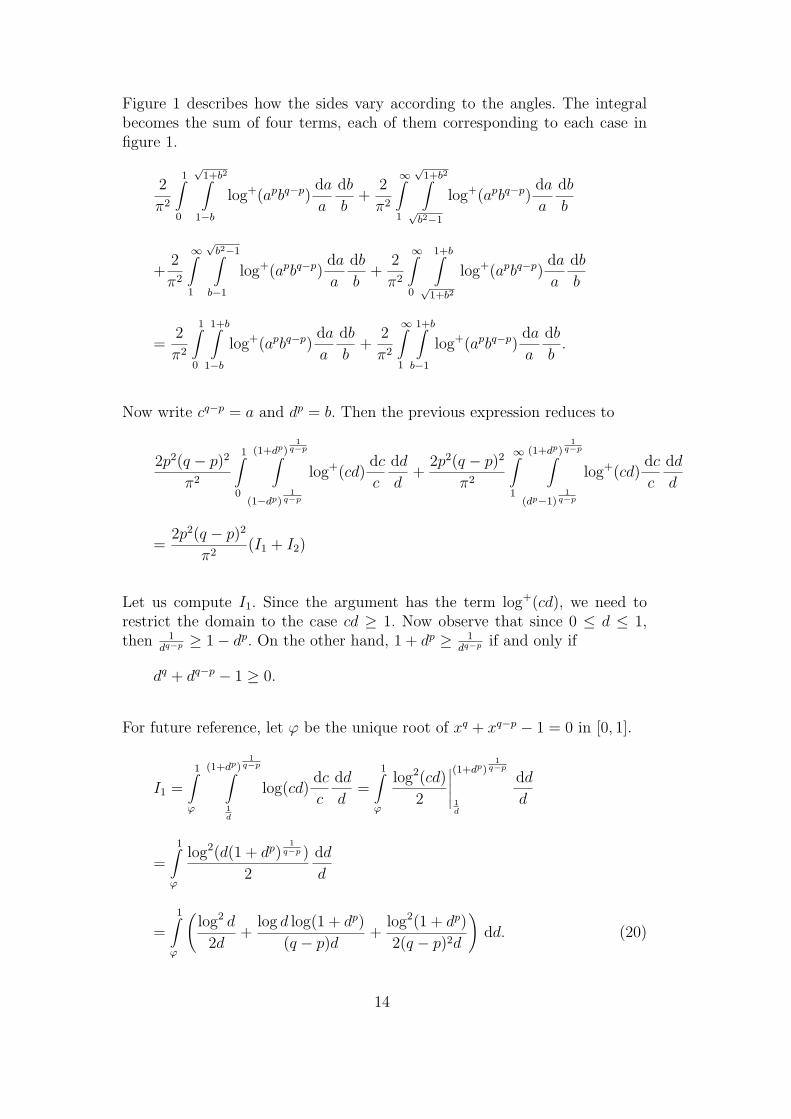
Figure 1 describes how the sides vary according to the angles. The integralbecomes the sum of four terms, each of them corresponding to each case infigure 1.

2

π2

1∫

0

√1+b2∫

1−b

log+(apbq−p)da

a

db

b+

2

π2

∞∫

1

√1+b2∫

√b2−1

log+(apbq−p)da

a

db

b

+2

π2

∞∫

1

√b2−1∫

b−1

log+(apbq−p)da

a

db

b+

2

π2

∞∫

0

1+b∫

√1+b2

log+(apbq−p)da

a

db

b

=2

π2

1∫

0

1+b∫

1−b

log+(apbq−p)da

a

db

b+

2

π2

∞∫

1

1+b∫

b−1

log+(apbq−p)da

a

db

b.

Now write cq−p = a and dp = b. Then the previous expression reduces to

2p2(q − p)2

π2

1∫

0

(1+dp)1

q−p∫

(1−dp)1

q−p

log+(cd)dc

c

dd

d+

2p2(q − p)2

π2

∞∫

1

(1+dp)1

q−p∫

(dp−1)1

q−p

log+(cd)dc

c

dd

d

=2p2(q − p)2

π2(I1 + I2)

Let us compute I1. Since the argument has the term log+(cd), we need torestrict the domain to the case cd ≥ 1. Now observe that since 0 ≤ d ≤ 1,then 1

dq−p ≥ 1− dp. On the other hand, 1 + dp ≥ 1dq−p if and only if

dq + dq−p − 1 ≥ 0.

For future reference, let ϕ be the unique root of xq + xq−p − 1 = 0 in [0, 1].

I1 =

1∫

ϕ

(1+dp)1

q−p∫

1d

log(cd)dc

c

dd

d=

1∫

ϕ

log2(cd)

2

∣∣∣∣∣

(1+dp)1

q−p

1d

dd

d

=

1∫

ϕ

log2(d(1 + dp)1

q−p )

2

dd

d

=

1∫

ϕ

(log2 d

2d+

log d log(1 + dp)

(q − p)d+

log2(1 + dp)

2(q − p)2d

)dd. (20)

14

The first term in the integral (20) is easy to integrate:

1∫

ϕ

log2 d

ddd = − log3 ϕ

3.

For the second term, we use the series expansion of log(1 + x):

1∫

ϕ

log d log(1 + dp)

ddd = −

1∫

ϕ

∞∑

l=1

(−1)l dpl−1

llog d dd

= −∞∑

l=1

(−1)l dpl

pl2log d

∣∣∣∣∣1

ϕ

+

1∫

ϕ

∞∑

l=1

(−1)l dpl−1

pl2dd

=log ϕ

pLi2(−ϕp) +

1

p2(Li3(−1)− Li3(−ϕp)).

We apply definition (10) to conclude that this expression equals

− 1

p2P3(−ϕp) +

(q − p) log3 ϕ

3− 3

4p2ζ(3).

Finally, we compute the third term of (20)

1∫

ϕ

log2(1 + dp)

ddd =

1

p

ϕq−p∫

12

log2 c

c(1− c)dc

(setting c = 11+dp )

=1

p

ϕq−p∫

12

log2 c(

1

c+

1

1− c

)dc

=(q − p)3 log3 ϕ

3p+

log3 2

3p− 1

plog2 c log(1− c)

∣∣∣∣∣ϕq−p

12

+1

p

ϕq−p∫

12

2 log c log(1− c)

cdc

15

= −(2q + p)(q − p)2 log3 ϕ

3p− 2 log3 2

3p− 2

p

∞∑

l=1

cl

l2log c

∣∣∣∣∣ϕq−p

12

+2

p

ϕq−p∫

12

∞∑

l=1

cl−1

l2dc

= −(2q + p)(q − p)2 log3 ϕ

3p− 2 log3 2

3p− 2(q − p)

plog ϕLi2(ϕ

q−p)

−2 log 2

pLi2

(1

2

)+

2

pLi3(ϕ

q−p)− 2

pLi3

(1

2

)

=2

pP3(ϕ

q−p)− (q − p)2 log3 ϕ

3− 2

pP3

(1

2

).

Then

I1 =1

p(q − p)2P3(ϕ

q−p)− 1

p2(q − p)P3(−ϕp)− 1

p(q − p)2P3

(1

2

)− 3ζ(3)

4p2(q − p).

Let us compute I2. As before, we need to restrict our domain to the casecd ≥ 1. Since 1 ≤ d, we have 1

dq−p ≤ 1 + dp always. On the other hand,dp − 1 ≥ 1

dq−p if and only if

dq − dq−p − 1 ≥ 0.

For future reference, let φ be the unique root of xq − xq−p − 1 = 0 in [1,∞).

Then

I2 =

φ∫

1

(1+dp)1

q−p∫

1d

log(cd)dc

c

dd

d+

∞∫

φ

(1+dp)1

q−p∫

(dp−1)1

q−p

log(cd)dc

c

dd

d= I21 + I22.

We proceed to compute I21,

I21 =

φ∫

1

log2(d(1 + dp)1

q−p )

2

dd

d=

1

(q − p)2

1∫

φ−1

(log(1 + cp)− q log c)2

2

dc

c

16

(setting c = 1d)

=1

(q − p)2

1∫

φ−1

(q2 log2 c

2c− q log c log(1 + cp)

c+

log2(1 + cp)

2c

)dc.

Using similar computations to those from I1, we obtain

I21 =q2 log3 φ

6(q − p)2+

q log2 φ log(

1+φp

φp

)

3(q − p)2+

log φ log2(

1+φp

φp

)

6(q − p)2+

q

p2(q − p)2P3

(− 1

φp

)

+1

p(q − p)2P3

(φp

1 + φp

)− 1

p(q − p)2P3

(1

2

)+

3qζ(3)

4p2(q − p)2.

For the case of I22 we have:

I22 =

∞∫

φ

log2(d(1 + dp)1

q−p )− log2(d(dp − 1)1

q−p )

2

dd

d

=1

(q − p)2

φ−1∫

0

(log2(1 + cp)

2c− log2(1− cp)

2c

+q log c log(1− cp)

c− q log c log(1 + cp)

c

)dc (21)

(setting c = 1d).

Now we compute each of the terms in equation (21):

φ−1∫

0

log2(1 + cp)

cdc = −

log2(

φp

1+φp

)log φ

3− 2

pP3

(φp

1 + φp

)+

2

pζ(3).

φ−1∫

0

log2(1− cp)

cdc =

1

p

1∫

φ−q

log2 f

1− fdf

(setting f = 1− cp)

= −1

plog2 f log(1− f)

∣∣∣1

φ−q+

1

p

1∫

φ−q

2 log f log(1− f)

fdf

17

= −q2 log3 φ− 2q

plog φLi2

(1

φq

)+

2

pζ(3)− 2

pLi3

(1

φq

)

= −q2 log3 φ

3− 2

pP3

(1

φq

)+

2

pζ(3).

φ−1∫

0

log c log(1− cp)

cdc =

log φ

pLi2

(1

φp

)+

1

p2Li3

(1

φp

)

=1

p2P3

(1

φp

)− q log3 φ

3.

φ−1∫

0

log c log(1 + cp)

cdc =

log φ

pLi2

(− 1

φp

)+

1

p2Li3

(− 1

φp

)

=1

p2P3

(− 1

φp

)+

log2 φ log(

1+φp

φp

)

3.

Putting all the terms together,

(q − p)2I22 = −log2

(φp

1+φp

)log φ

6− q2 log3 φ

6−

q log2 φ log(

1+φp

φp

)

3

−1

pP3

(φp

1 + φp

)+

1

pP3

(1

φq

)+

q

p2P3

(1

φp

)− q

p2P3

(− 1

φp

)

and hence,

(q − p)2I2 = −1

pP3

(1

2

)+

3qζ(3)

4p2+

1

pP3

(1

φq

)+

q

p2P3

(1

φp

).

Now we can conclude:

I1 + I2 =1

p(q − p)2P3(ϕ

q−p)− 1

p2(q − p)P3(−ϕp)

− 2

p(q − p)2P3

(1

2

)+

3ζ(3)

4p(q − p)2+

1

p(q − p)2P3 (φq) +

q

p2(q − p)2P3 (φp) .

Let us note that 2P3

(12

)+ P3(−1) = ζ(3) because of equation (15), hence,

P3

(1

2

)=

7

8ζ(3).

18

Then

I1 + I2 =1

p(q − p)2P3(ϕ

q−p)− 1

p2(q − p)P3(−ϕp)

− ζ(3)

p(q − p)2+

1

p(q − p)2P3 (φq) +

q

p2(q − p)2P3 (φp) .

Now, we use equation (15) again in order to obtain P3(ϕq) + P3(1 − ϕq) +

P3(1− ϕ−q) = ζ(3) from where

P3(ϕq) + P3(ϕ

q−p) + P3(−ϕ−p) = ζ(3),

so

P3(ϕq−p) = ζ(3)− P3(−ϕp)− P3(ϕ

q).

Hence, we have

I1 + I2 = − 1

p(q − p)2P3(ϕ

q)− q

p2(q − p)2P3(−ϕp)

+1

p(q − p)2P3 (φq) +

q

p2(q − p)2P3 (φp) ,

which proves our claim.

4 An example in dimension 4

We would like to study one more example, which is a particular case of a4-dimensional resultant. Let us set n = 2 and

A0 = A1 = A2 = A := {(0, 0), (1, 0), (0, 1)}.We will use a formula due to Cassaigne and Maillot

Theorem 4.1 [Mai, Proposition 7.3.1],

πm(a + bx + cy) =

D(∣∣∣a

b

∣∣∣ eiγ)

+ α log |a|+ β log |b|+ γ log |c| if4

π log max{|a|, |b|, |c|} if not4(22)

19

Where 4 stands for the statement that |a|, |b|, and |c| are the lengths of thesides of a triangle; and α, β, and γ are the angles that are opposite to thesides of lengths |a|, |b| and |c| respectively.

Theorem 7 m(ResA,A,A) =9ζ(3)

2π2.

PROOF. In order to simplify the notation, we will use the variables a, b, c, . . .instead of the xij’s.

ResA,A,A = det

a b c

d e f

g h i

.

Now, let us proceed to eliminate homogeneous variables:

m

∣∣∣∣∣∣∣∣∣∣∣

a b c

d e f

g h i

∣∣∣∣∣∣∣∣∣∣∣

= m

∣∣∣∣∣∣∣∣∣∣∣

1 1 1

d e f

g h i

∣∣∣∣∣∣∣∣∣∣∣

= m

∣∣∣∣∣∣∣∣∣∣∣

1 1 1

1 e f

1 h i

∣∣∣∣∣∣∣∣∣∣∣

= m

∣∣∣∣∣∣∣∣∣∣∣

1 0 0

1 e− 1 f − 1

1 h− 1 i− 1

∣∣∣∣∣∣∣∣∣∣∣

= m((e− 1)(i− 1)− (f − 1)(h− 1)).

Let us observe that

m((x− 1)(y − 1)− (z − 1)(w − 1)) = m((x− 1)y + (1− z)w + (z − x)).(23)

Hence we can think of the polynomial (x− 1)y +(1− z)w +(z−x) as a linearpolynomial in the variables y, w, whose coefficients are in Z[x, z]. Because ofthe iterative nature of the definition of Mahler measure, we can choose to in-tegrate first respect to the variables y and w, regarding x and z as parameters.If we do that, we obtain formula (22) with the sides of the triangle equal to|x− 1|, |z − 1|, and |z − x|.

Now in order to compute the Mahler measure, we still need to integrate thisformula respect to x and z. Set x = e2iα and z = e2iβ. This notation isconsistent with the names for the angles of the triangle because of the SineTheorem (see Figure 2).

20

| z − 1 | = 2 | sin ( β ) || z − x | = 2 | sin ( β − α ) | α

β − απ − β

| x − 1 | = 2 | sin ( α ) |

Fig. 2. We always obtain a triangle for this case.

We obtain that (23) is equal to

2

π3

π∫

0

β∫

0

D

(sin β

sin αei(β−α)

)+ α log |2 sin α|+ (β − α) log |2 sin(β − α)|

+(π − β) log |2 sin β| dα dβ.

First, we integrate the terms involving logarithms:

π∫

0

π∫

α

α log |2 sin α| dβ dα =

π∫

0

α(π − α) log |2 sin α| dα

=

π∫

0

α(π − α) log∣∣∣1− e2iα

∣∣∣ dα = −π∫

0

α(π − α) Re∞∑

j=1

e2jiα

jdα.

Because of

π∫

0

(πα− α2)cos(2jα)

jdα = (πα− α2)

sin(2jα)

2j2

∣∣∣∣∣π

0

−π∫

0

(π − 2α)sin(2jα)

2j2dα

= (π − 2α)cos(2jα)

4j3

∣∣∣∣∣π

0

−π∫

0

(−2)cos(2jα)

4j3dα = − π

2j3,

we conclude that

π∫

0

α(π − α) log |2 sin α| dα =πζ(3)

2.

Then

π∫

0

β∫

0

(π − β) log |2 sin β| dα dβ =

π∫

0

β(π − β) log |2 sin β| dβ =πζ(3)

2,

21

by analogy with the case of α.

By setting γ = β − α in the third logarithmic term,

π∫

0

β∫

0

(β − α) log |2 sin(β − α)| dα dβ =

π∫

0

π−γ∫

0

γ log |2 sin γ| dα dγ

=

π∫

0

γ(π − γ) log |2 sin γ| dγ =πζ(3)

2.

On the other hand, we need to evaluate

π∫

0

β∫

0

D

(sin β

sin αei(β−α)

)dα dβ. (24)

Using equation (12),

D

(sin β

sin αei(β−α)

)= D

(1− z

1− x

)=

1

2

(D

(z

x

)+ D(x) + D

(1

z

))

=1

2

(D(e2i(β−α)) + D(e2iα) + D(e−2iβ)

).

Then integral (24) is the sum of three terms. We proceed to compute each ofthem:

π∫

0

π∫

α

D(e2iα) dβ dα =

π∫

0

(π − α)D(e2iα) dα

=

π∫

0

(π − α)∞∑

j=1

sin(2jα)

j2dα.

But

π∫

0

(π − α)sin(2jα)

j2dα = −(π − α)

cos(2jα)

2j3

∣∣∣∣∣π

0

−π∫

0

cos(2jα)

2j3dα =

π

2j3.

Then

π∫

0

(π − α)D(e2iα) dα =πζ(3)

2.

22

The other terms can be computed in a similar fashion:

π∫

0

β∫

0

D(e−2iβ) dα dβ = −π∫

0

βD(e2iβ) dβ =πζ(3)

2,

π∫

0

β∫

0

D(e2i(β−α)) dα dβ =

π∫

0

π−γ∫

0

D(e2iγ) dα dγ

=

π∫

0

(π − γ)D(e2iγ) dγ =πζ(3)

2.

Thus, we conclude that

m((x− 1)(y − 1)− (z − 1)(w − 1)) =2

π3

(3

2

πζ(3)

2+ 3

πζ(3)

2

)=

9ζ(3)

2π2.

5 Resultants are tempered polynomials

In this section we will leave the elementary approach given above and turninstead to study algebraic properties of resultants and Mahler measures in thecontext of Milnor K-theory. We will sketch the relation here and we refer to[Den], [RV], and [Lal2] for precise details.

For P ∈ C[s1, . . . , sp] irreducible, we write

P (s1, . . . , sp) =∑

i≥0

ai(s1, . . . , sp−1)sip.

Let

P ∗(s1, . . . , sp−1) = ai0(s1, . . . , sp−1),

the main non-zero coefficient respect to sp. Let X be the zero set {P (s1, . . . , sp) =0}.

By applying Jensen’s formula to the Mahler measure of P respect to thevariable sp, it is possible to write

m(P ) = m(P ∗)− 1

(2iπ)p−1

∫

Γ

log |sp| ds1

s1

. . .dsp−1

sp−1

23

where Γ = {P (s1, . . . , sp) = 0} ∩ {|s1| = . . . = |sp−1| = 1, |sp| ≥ 1}.

From this formula, Deninger [Den] establishes

m(P ) = m(P ∗)− 1

(2iπ)p−1

∫

Γ

η(s1, . . . , sp) (25)

where η(s1, . . . , sp) is certain R(p− 1)-valued smooth p− 1-form in X (C) \ S.Here, S denotes the set of poles and zeros of the functions s1, . . . , sp.

For example, in two variables, η has the following shape:

η(x, y) = log |y|i d arg x− log |x|i d arg y.

η is a closed form that is multiplicative and antisymmetric in the variabless1, . . . sp. Therefore, it is natural to think of η as a function on

∧pC(X ) ⊗Q (we tensorize by Q because η is trivial in torsion elements). Even more,η(1− s, s, s3, . . . , sp) is an exact form. We may also see η(s1, . . . , sp) as a classin the (DeRham) cohomology of X \ S. This situation allows us to thinkof the cohomological class of η as a function in the Milnor K-theory groupKM

p (C(X ))⊗Q. Recall that for a field F the Milnor K-theory group is givenby

KMp (F ) :=

p∧F ∗/ 〈(1− s1) ∧ s1 ∧ . . . ∧ sp, si ∈ F ∗〉

If we can extend this class to the cohomology of X , η becomes a regulator. Incertain cases, seeing the Mahler measure as a regulator allows us to explain itsrelation to special values of L-functions via Beilinson’s conjectures and similarresults.

The condition that the class of η(s1, . . . , sp) be extended to X is given by thetriviality of the tame symbols in the Milnor K-theory. A stronger condition isthat η(s1, . . . , sp) is exact. Since η is defined in KM

p (C(X ))⊗Q, η(s1, . . . , sp)is exact if the symbol {s1, . . . , sp} is trivial in KM

p (C(X ))⊗Q.

This is a very special condition that is not true for a general polynomial.However, it is true for resultants:

Theorem 8 The symbol

{x01, . . . , x0k0 , . . . , xn1, . . . , xnkn} ∈ KMk (C(X ))⊗Q (26)

is trivial.

24

In order to prove Theorem 8, we will need the following

Lemma 9 Consider a p-variable polynomial

P (u1, . . . , up) :=∑

xiui.

Here i is a multiindex, ui = ui11 . . . uip

p .

Let E be a field containing the x′is and let α1, . . . αp in E. Then∧

xi is of theform

P (α1, . . . , αp) ∧∧

ai +∑

i,h

ri,hαi ∧∧

ci,h +∑

j,l

sj,lbj ∧ (1− bj) ∧∧

b′j,l,

where ai, bj, b′j,l, ci,h are elements of E and ri,h, sj,l are integral numbers.

PROOF. First we prove the case for which p = 1. Let us write

P (α) = x0

(1 +

x1

x0

α

(1 +

x2

x1

α . . .

(1 +

xq

xq−1

α

))).

After setting y0 = x0 and yi = xi

xi−1for i > 0, we obtain

P (α) = y0(1 + y1α(1 + y2α . . . (1 + yqα))),

and

x0 ∧ . . . ∧ xq = y0 ∧ . . . ∧ yq.

We may introduce α in the last place of the wedge product of yi:

y0 ∧ . . . ∧ yq = y0 ∧ . . . ∧ yq−1 ∧ (yqα)− y0 ∧ . . . ∧ yq−1 ∧ α.

Now we introduce α in the second to the last place

= y0 ∧ . . . ∧ yq−1(1 + yqα) ∧ (yqα)− y0 ∧ . . . ∧ (1 + yqα) ∧ (yqα)

−y0 ∧ . . . ∧ yq−1 ∧ α

= y0 ∧ . . . ∧ yq−2 ∧ yq−1α(1 + yqα) ∧ (yqα)− y0 ∧ . . . ∧ yq−2 ∧ α ∧ yq

−y0 ∧ . . . ∧ (1 + yqα) ∧ (yqα)− y0 ∧ . . . ∧ yq−1 ∧ α.

25

Then we introduce α in the third to the last place. We continue in this fashion

= y0 ∧ . . . ∧ yq−2(1 + yq−1α(1 + yqα)) ∧ yq−1α(1 + yqα) ∧ (yqα)

−y0 ∧ . . . ∧ (1 + yq−1α(1 + yqα)) ∧ yq−1α(1 + yqα) ∧ (yqα)

−y0 ∧ . . . ∧ yq−2 ∧ α ∧ yq − y0 ∧ . . . ∧ (1 + yqα) ∧ (yqα)

−y0 ∧ . . . ∧ yq−1 ∧ α.

After q − 1 more steps, we get

P (α) ∧∧ai +

q∑

h=1

±(bh ∧ (1− bh) ∧∧

b′h,l)

−q∑

h=1

y0 ∧ . . . ∧ yh−1 ∧ α ∧ yh+1 ∧ . . . ∧ yq,

which proves the claim in this case.

Let us now consider p > 1. We use induction on p. Suppose that the claim istrue for p− 1. Then we may write

P (α1, . . . , αp) =∑

Pi(α1, . . . , αp−1)αip.

By the inductive hypothesis we obtain

∧xi = P0(α1, . . . , αp−1) ∧ . . . ∧ Ph(α1, . . . , αp−1) ∧

∧ai

+∑

i,h

ri,hαi ∧∧

ci,h +∑

j,l

sj,lbj ∧ (1− bj) ∧∧

b′j,l.

Now apply the case p = 1 to the first term in order to obtain the desiredresult.

In the notation of this proof we used that the coefficients were all differentfrom zero. The proof is easily adapted to the case when some coefficients arezero. We are going to use this lemma in full generality.

PROOF (Theorem 8) By definition of Milnor’s K-theory, it is sufficient towork in

∧k C(X )∗ ⊗Q. Consider the variety

Y = {z − ResA0,...,An = 0} ⊂ Ck+1.

26

Let H := C(Y) and E be a finite extension of H containing all the roots thatare common to the last n polynomials F1, . . . , Fn in an algebraically closedfield containing H.

We will prove that the symbol determined by

z ∧∧x0j ∧

∧x1j ∧ . . . ∧∧

xnj

is trivial in∧k+1 E∗ ⊗ Q. This fact implies that the corresponding symbol in

KMk+1(E)⊗Q is trivial. Now j : H ↪→ E induces j : KM

∗ (H) → KM∗ (E) whose

kernel is finite (see [BT]). Then KM∗ (H)⊗Q ↪→ KM

∗ (E)⊗Q is injective andwe conclude that the symbol must be trivial in

∧k+1 H∗ ⊗Q.

The triviality of this symbol implies that∧

x0j ∧∧

x1j ∧ . . . ∧∧xnj

is trivial in∧sC(X )∗⊗Q, because it is the image by the tame symbol morphism

respect to the valuation determined by z = 0, [Mil] (in the language of Newtonpolytopes, ResA0,...,An corresponds to a facet of z − ResA0,...,An).

We will use the Poisson product formula for sparse resultants (Theorem 1.1in [PS] and its refinement in [Min, Theorem 8]):

ResA0,...,An =∏η

Resηdη

∏

α

F0(α), (27)

where η runs over all the maximal facets of the Newton polytope associated tothe Minkowski sum A1+. . .+An, Resη stands for the facet resultant associatedto (1) and the facet η, dη is a non negative integer number, and α runs overall the common solutions of the system F1 = . . . = Fn = 0 in (E \ {0})n .

Let us proceed by induction on n. For n = 1 we have, F0 = x01ta011 + . . . +

x0k0ta0k01 and F1 = x11t

a111 + . . . + x1k1t

a1k11 , where we assume w.l.o.g. that

a01 < a02 < . . . < a0k0 and a11 < a12 < . . . < a1k1 . Also, we can supposew.l.o.g. that a01 = a11 = 0. This is due to the fact that the resultant isinvariant under translations of the Ai’s. Then,

Res(F0, F1) = xd1k1

∏F0(α),

where α runs over the roots of F1 in E \ {0}, and d is a positive integer. LetF1 := x12t

a121 + . . . + x1k1t

a1k11 . Then

z ∧∧x0j ∧

∧x1j =

∑F0(α) ∧

k0∧

j=1

x0j ∧ F1(α) ∧k1∧

j=2

x1j

27

+d x1k1 ∧k0∧

j=1

x0j ∧ F1(α) ∧k1∧

j=2

x1j.

The second term is zero because it contains two copies of x1k1 . By applyingLemma 9, the first term yields a combination of terms of the form bj ∧ (1 −bj) ∧ ∧

b′j,l, which is trivial in K-theory.

Now let n > 1, and assume again w.l.o.g. that all the supportsAi are containedin Nn, so the Fi’s are Taylor polynomials and we can use Lemma 9. Fix asolution α = (α1 . . . , αn) in (E \ {0})n for the last n equations. As in the casen = 1, it is easy to see that we may write equations of the kind

xl1 = a−1Fl(α)

where a is equal to a product (possibly empty) of αi.

We need to consider

z ∧∧x0j ∧

∧x1j ∧ . . . ∧∧

xnj,

which, due to (27), equals

∑F0(α) ∧

k0∧

j=1

x0j ∧ F1(α) ∧k1∧

j=2

x1j ∧ . . . ∧ Fn(α) ∧kn∧

j=2

xnj

+∑η

dη Resη ∧k0∧

j=1

x0j ∧ F1(α) ∧k1∧

j=2

x1j ∧ . . . ∧ Fn(α) ∧kn∧

j=2

xnj

The sum is over all the solutions α of Fi = 0 for 1 ≤ i ≤ n.

For the first term, we apply Lemma 9 to each of the n + 1 sets of coefficientsand obtain a combination of terms of the form bj ∧ (1 − bj) ∧ ∧

b′j,l, which istrivial in K-theory.

The terms that correspond to combinations of αi ∧ ∧ci,h are zero because we

have n different αi’s but n+1 terms, which means that some αi appears twicein the wedge product and then it must be equal to zero.

Consider the second term. For each η and i = 1 . . . , n, we define Gηi := F η

i ,the restriction of Fi to the facet η (see [PS] for a precise definition definitionof these polynomials). As the coefficients of the Gη

i ’s are included in the coeffi-cients of the Fi, we can apply induction and obtain the triviality of this term.This can be done due to the fact that Resη is always a resultant associated to a

28

system of dimension n−1 or less. Hence, the symbol is trivial in KMk+1(E)⊗Q

and that proves the claim.

Acknowledgements

The authors wish to thank Fernando Rodriguez-Villegas for several suggestionsand also Martın Sombra for explaining to them his work [Som2]. They wouldalso like to express their gratitude to the Miller Institute at UC Berkeleyand the Department of Mathematics at the University of Texas at Austin fortheir support. Matilde Lalın is also grateful to the Harrington fellowship andJohn Tate for their support. The authors are grateful to the Referee for theirsuggestions.

References

[BT] Bass, Hyman; Tate, John. The Milnor ring of a global field. AlgebraicK-theory, II: “Classical” algebraic K-theory and connections witharithmetic (Proc. Conf., Seattle, Wash., Battelle Memorial Inst., 1972),pp. 349–446. Lecture Notes in Math., Vol. 342, Springer, Berlin, 1973.

[Boy] Boyd, David. Speculations concerning the range of Mahler’s measure.Canad. Math. Bull. 24 (1981), 453–469.

[CLO] Cox, David; Little, John; O’Shea, Donal. Using algebraic geometry.Graduate Texts in Mathematics, 185. Springer-Verlag, New York, 1998.

[DAn] D’Andrea, Carlos. Macaulay style formulas for sparse resultants. Trans.Amer. Math. Soc. 354 (2002), no. 7, 2595–2629.

[Den] Deninger, Christopher. Deligne periods of mixed motives, K-theory andthe entropy of certain Zn-actions. J. Amer. Math. Soc. 10 (1997), no. 2,259–281.

[DH] D’Andrea, Carlos; Hare, Kevin. On the height of the Sylvester resultant.Experiment. Math. 13 (2004), no. 3, 331–341.

[EM] Emiris, Ioannis Z.; Mourrain, Bernard. Matrices in elimination theory.Polynomial elimination—algorithms and applications. J. SymbolicComput. 28 (1999), no. 1-2, 3–44.

[EW] Everest, Graham; Ward, Thomas. Heights of polynomials and entropy inalgebraic dynamics. Universitext. Springer-Verlag London, Ltd., London,1999.

29

[Khe] Khetan, Amit. The resultant of an unmixed bivariate system.International Symposium on Symbolic and Algebraic Computation(ISSAC’2002) (Lille). J. Symbolic Comput. 36 (2003), no. 3-4, 425–442.

[KPS] Krick, Teresa; Pardo, Luis Miguel; Sombra, Martın. Sharp estimates forthe arithmetic Nullstellensatz. Duke Math. J. 109 (2001), no. 3, 521–598.

[Lal] Lalın, Matilde. Some examples of Mahler measures as multiplepolylogarithms. J. Number Theory 103 (2003), no. 1, 85–108.

[Lal2] Lalın, Matilde. An algebraic integration for Mahler measure. Preprint.

[Mai] Maillot, Vincent Geometrie d’Arakelov des varietes toriques et fibres endroites integrables. Mem. Soc. Math. Fr. (N.S.), 80 (2000) 129pp.

[Mil] Milnor, John. Algebraic K-theory and quadratic forms. Invent. Math. 91969/1970 318–344.

[Min] Minimair, Manfred. Sparse resultant under vanishing coefficients. J.Algebraic Combin. 18 (2003), no. 1, 53–73.

[PS] Pedersen, Paul; Sturmfels, Bernd. Product formulas for resultants andChow forms. Math. Z. 214 (1993), no. 3, 377–396.

[RV] Rodriguez-Villegas, Fernando. Modular Mahler measures I. Topics innumber theory (University Park, PA 1997), 17–48, Math. Appl., 467,Kluwer Acad. Publ. Dordrecht, 1999.

[R-VTV] Rodriguez-Villegas, Fernando; Toledano, Ricardo; Vaaler, Jeffrey.Estimates for Mahler’s measure of a linear form. Proc. Edinb. Math.Soc. (2) 47 (2004), no. 2, 473–494.

[Smy1] Smyth, Christopher J. On measures of polynomials in several variables.Bull. Austral. Math. Soc. 23 (1981), no. 1, 49–63. Corrigendum: MyersonG.;Smyth, C. J. 26 (1982), 317–319.

[Smy2] Smyth, Christopher J. An explicit formula for the Mahler measure of afamily of 3-variable polynomials. J. Th. Nombres Bordeaux 14 (2002),683–700.

[Som1] Sombra, Martın. Estimaciones para el Teorema de Ceros de Hilbert. Tesisde Doctorado, Departamento de Matematica, Universidad de BuenosAires, 1998.

[Som2] Sombra, Martın. The height of the Mixed Sparse resultant. Amer. J.Math. 126 (2004), no. 6, 1253–1260.

[Stu] Sturmfels, Bernd. On the Newton polytope of the resultant. J. AlgebraicCombin. 3 (1994), no. 2, 207–236.

[Zag1] Zagier, Don. The Dilogarithm function in Geometry and Number Theory.Number Theory and related topics, Tata Inst. Fund. Res. Stud. Math.,12, Bombay (1988), 231– 249.

30

[Zag2] Zagier, Don. Polylogarithms, Dedekind zeta functions and the algebraicK-theory of fields. Arithmetic algebraic geometry (Texel, 1989), 391–430,Progr. Math., 89, Birkhauser Boston, Boston, MA, 1991.

31