
"In pursuit of preparing tomorrow's technologists" On Job Training Report Training Organization
Upload
khangminh22Category
view
1download
0
Upjohn Press Upjohn Research home page
1-1-1997
On-the-Job Training On-the-Job Training
John M. Barron Purdue University
Mark C. Berger University of Kentucky
Dan A. Black University of Kentucky
Follow this and additional works at: https://research.upjohn.org/up_press
Part of the Labor Economics Commons
Citation Citation Barron, John M., Mark C. Berger, and Dan A. Black. 1997. On-the-Job Training. Kalamazoo, MI: W.E. Upjohn Institute for Employment Research. https://doi.org/10.17848/9780585262369
This work is licensed under a Creative Commons Attribution-Noncommercial-Share Alike 4.0 License.
This title is brought to you by the Upjohn Institute. For more information, please contact [email protected].

JOHN M. BARRONMARK C. BERGER
DAN A. BLACK


ON-THE-JOBTRAINING
John M. BarrenPurdue University
Mark C. BergerUniversity of Kentucky
Dan A. BlackUniversity of Kentucky
1997
W.E. Upjohn Institute for Employment Research Kalamazoo, Michigan

Library of Congress Cataloging-in-Publication Data
Barren, John M. On the job training / John M. Barron, Mark C. Berger, Dan A. Black.
p. cm.Includes bibliographical references and index. ISBN 0-88099-178-X (cloth : alk. paper). ISBN 0-88099-175-5
(pbk.: alk. paper)1. Employees,Training of Evaluation. 2. Organizational
learning. I. Berger, Mark C. II. Black, Dan A. III. Title. HF5549.5.T7B2917 1997658.3©12404 dc21 97-10295
CIP
Copyright 1997 W. E. Upjohn Institute for Employment Research
300 S. Westnedge Avenue Kalamazoo, Michigan 49007^4686
The facts presented in this study and the observations and viewpoints expressed are the sole responsibility of the authors. They do not©necessarily represent positions of the W. E. Upjohn Institute for Employment Research.
Cover design by J. R. Underhill Index prepared by Shirley Kessel. Printed in the United States of America.

Acknowledgments
We would like to express thanks to the many individuals and organizations that have helped make this research possible. We wish to thank the W.E. Upjohn Institute for Employment Research for financial support for conduct ing this research. We also thank the U.S. Small Business Administration for financial support to conduct the SBA survey (Contract No. SBA-6640-OA- 91). The SBA and Upjohn Institute Surveys were conducted ably by the Sur vey Research Center at the University of Kentucky. We especially thank Jim Wolf for his help with questionnaire design and Melissa Huffman for assis tance in the initial processing of the survey data. We thank Kevin Hollenbeck for many useful comments and suggestions throughout the entire project and Don Parsons for his thorough review of the completed draft of the manuscript. We also received helpful comments from seminar participants at the Upjohn Institute for Employment Research. We appreciate the patience and endurance of Steve Alien and Amitabh Chandra, who read and provided comments on countless versions of various chapters. We thank Judy Gentry for her editing of the final manuscript.

The Authors
John M. Barren is a professor in the Department of Economics, Krannert Graduate School of Management, Purdue University. He received a Ph.D. in economics from Brown University in 1976. His research areas include labor economics, the economics of information and uncertainty, and applied micro economics, and he has published many scholarly papers in these areas. In 1987 he was a visiting professor at the University of Essex and London School of Economics, and in 1995 he was a visiting professor at Royal Holloway, University of London.
Mark C. Berger is a professor of economics, an Ashland Oil Research Fellow, and the director of the Center for Business and Economic Research in the Gat- ton College of Business and Economics at the University of Kentucky. He received a Ph.D. in economics from The Ohio State University in 1981. He has published many scholarly papers in the areas of labor economics, health economics, and public policy. In 1987-88 he was a Research Fellow at the National Opinion Research Center of the University of Chicago, and in 1996 he was a visiting professor at the Economics University of Vienna, Austria.
Dan Black is a professor of economics and an Ashland Oil Research Fellow in the Gatton College of Business and Economics at the University of Kentucky. This year, he is on sabbatical leave to the Heinz School at Carnegie Mellon University where he is a visiting professor of Public Policy. In 1989-90, he was a visiting associate professor at the Harris School of Public Policy Studies at the University of Chicago. He received his Ph.D. from Purdue University in 1983. His major research areas are labor economics and public policy, and he has published numerous papers and two books in these areas.

CONTENTS
1 Introduction 1Note 3
2 On-the-job Training as an Investment in Human Capital 5A Simple Model of On-the-Job Training 6 Traditional Predicted Effects of Training on Wages,
Productivity, and Turnover 12Other Models of Compensation, Productivity, and Turnover 19 Evidence Concerning the Standard Predictions
of On-the-Job Training 22Notes 28
3 Measures of On-the-Job Training 31Employer Survey Questions on Training 31Employer Measures of On-the-Job Training 34Worker Measures of On-the-Job Training 41Conclusions 48Notes 49
4 Who Receives On-the-Job Training? 51Variations in the Level of Training 52Variations in the Incidence of Training 68Truncated Spells of Training 75Conclusions 81Notes 82
5 How Well Do We Measure On-the-Job Training? 85Previous Validation Studies in Labor Economics 86A New Validation Survey 90 Correlations Between Employer and Employee Reports
and Comparisons with the Results of Previous Studies 93Measures of On-the-Job Training 104 Determinants of Training and Reported Differences in Training 108Conclusions 111Notes 114
6 The Impact of Training on Wages and Productivity 115Alternative Theories of Wage Growth 116On-the-Job Training Effects on the Starting Wage 118
Contrasting On-the-Job Training Impact on WagesVersus Productivity 130
Further Evidence on Wage and Productivity Growth 135 The Effect of Measurement Error on the Estimated Effect
of Training on Wages and Productivity? 137Why is the Impact of Training on the Starting Wage so Small? 141Notes 146
Appendix to Chapter 6 149Note 150
7 Training and Firm Recruiting Strategies 153Employer Optimal Search Strategy 155The Evidence on Employer Search Behavior 161The Evidence on Vacancy Duration 176Conclusions 180Notes 182
8 Conclusions 185Note 190
References 191
Index 201

List of Tables
3.1 Means and Incidence Rates of Training Measures, 1992 SB AData and 1982 EOPP Data 35
3.2 Comparison of 1992 SBA and 1982 EOPP Training Measures 373.3 Rates of Training Spells Lasting at Least 12 Weeks,
1992 SBA Data 383.4 Length of Time to Become Fully Trained and Qualified,
1992 SBA Data and 1982 EOPP Data 39
4.1 Means for the 1992 SBA and 1982 EOPP Data 584.2 Total Hours of Training for the 1992 SBA
and 1982 EOPP Data 594.3 Time to Become Fully Trained and Qualified for the 1992 SBA
and 1982 EOPP Data 634.4 Total Hours of Training for the 1992 SBA Data, Cox Model 674.5 Incidence of Off-Site Formal Training for the 1992 SBA Data 694.6 Incidence of On-Site Formal Training for the 1992 SBA
and 1982 EOPP Data 704.7 Incidence of Informal Management Training for the 1992 SBA
and 1982 EOPP Data 734.8 Incidence of Informal Co-Worker Training for the 1992 SBA
and 1982 EOPP Data 744.9 Incidence of Training by Watching Others for the 1992 SBA
and 1982 EOPP Data 764.10 Incidence of Training Spells Lasting at Least 12 Weeks
for the!992 SBA Data 78
5.1 Correlation between Worker and Firm Responses 955.2 Employer and Employee Measures of Hours of Training 1055.3 Employer and Employee Measures of Hours of Formal
and Informal Training 1065.4 Employer and Employee Measures of Training Incidence Rates 1075.5 Regression Explaining Levels of Training and Worker-Firm
Differences in Reported Training 109
6.1 Training and Starting Wage, 1992 SBA Data (percent) 1226.2 Impact of Training Proxies on the Starting Wage,
1992 SBA Data 1246.3 The Impact of Training on the Starting Wage, 1992 SBA
and 1982 EOPP Data 128

6.4 Wage and Productivity Index Growth, 1992 SB Aand 1982 EOPP Data 133
6.5 A Comparison of Productivity and Wage Index, 1992 SBA Dataand 1982 EOPP Data 135
6.6 Wage and Productivity Growth in the First 3 Monthsof Employment, 1992 SBA Data 136
6.7 Estimates of the Impact of Training on Starting Wages, andWage and Productivity Growth 139
6.8 The Degree to Which Skills are General, 1982 EOPP Data 142 A.6.1 Wage Equation Estimates (Ordinary Least Squares) Using the
1992 March Current Population Survey and the 1990 Census 151
7.1 Employer Search, Vacancy Duration, and Training Variables by Size, 1980 EOPP; 1982 EOPP; 1992 SBA;1993 Upjohn Institute Surveys 163
7.2 Determinants of Employer Search, 1980 EOPP Survey 1667.3 Determinants of Employer Search, 1982 EOPP Survey 1687.4 Determinants of Employer Search, 1992 SBA Survey 1707.5 Determinants of Employer Search, 1993 Upjohn Institute Survey 1727.6 Summary of Findings Concerning Determinants of Employer
Search and Vacancy Duration Across Four Surveys 1747.7 Vacancy Duration Models 1797.8 Employer Search and Unemployment Duration 181
Vlll

List of Figures
2.1 Effect of Training on Wage Profiles 14
3.1 EOPP and SB A Measures of Average Hours Spent inOn-the-Job Training During First Three Months 36
4.1 Hours of Training in the First Three Months of Employment,1992 SB A Data 52
4.2 Number of Weeks to Become Fully Trained and Qualified,1992 SBA Data 53
4.3 Hours of Training in the First Three Months of Employmentby Experience Level, 1992 SBA Data 54
4.4 Time to Become Fully Trained and Qualified by ExperienceLevel, 1992 SBA Data 54
4.5 Hours of Training in the First Three Months of Employmentby Establishment Size, 1992 SBA Data 55
4.6 Time to Become Fully Trained and Qualified by Race andGender, 1992 SBA Data 56
5.1 Firm-and Worker-Reported Wages 875.2 Firm- and Worker-Reported Hours Worked 875.3 Firm-and Worker-Reported Experience 885.4 Firm-and Worker-Reported Training 88
6.1 Human Capital Production Function 126
7.1 Vacancy Duration Hazard Rates (duration in days) 178


ON-THE-JOBTRAINING


CHAPTER 1
Introduction
In 1964, Gary Becker noted the important role of on-the-job training in Human Capital: A Theoretical and Empirical Analysis, with Special Reference to Education by observing that:
Theories of firm behavior, no matter how they differ in other respects, almost invariably ignore the effect of the productive pro cess itself on worker productivity. This is not to say that no one recognizes that productivity is affected by the job itself; but the recognition has not been formalized, incorporated into economic analysis, and its implications worked out.... Many workers increase their productivity by learning new skills and perfecting old ones while on the job. Presumably, future productivity can be improved only at a cost, for otherwise there would be an unlimited demand for training (1964, p. 8).
In the decades following Decker©s classic text, researchers have made substantial progress in achieving Becker©s goal of fully incorpo rating the role of on-the-job training into economic analysis.
Researchers now widely accept that there are two key aspects of training. First, there is the recognition that on-the-job training is an important example of an "investment" in human capital. 1 Like any investment, there are initial costs. For on-the-job training, these costs include the time devoted by the worker and co-workers to learning skills that increase productivity plus the costs of any equipment and material required to teach these skills. Like any investment, the returns to these expenditures occur in future periods. For on-the-job training, these future returns are measured by the increased productivity of the worker during subsequent periods of employment.
The second key aspect of on-the-job training is the distinction between "general" and "specific" on-the-job training, a distinction emphasized by Becker in his early works. While all training increases

2 Introduction
the productivity of the worker at the firm providing the training, gen eral training also increases the productivity of the worker at firms other than the one providing the training. For example, a secretary who learns the use of a standard word-processing program or a doctor who interns at a specific hospital both receive general training, as these skills are transferable to other workplaces. On the other hand, specific on-the-job training increases the productivity of the worker at the firm providing the training, but not at other firms. Resources spent orienting new employees to the practices of their new employer, or teaching employees how to contribute to a unique assembly process or work team, are examples of specific training.
Chapter 2 presents the standard theoretical framework for assessing the impact of on-the-job training on productivity, wages, and turnover. This sets the stage for our investigation in subsequent chapters of the magnitude and effects of on-the-job training, an investigation that focuses on three employer-based surveys of the training received by newly hired workers. We start by considering two questions: Exactly how much training do employers provide their workers? Who receives this training? Chapters 3 and 4 address these two issues: the extent of training and the characteristics of the recipients of on-the-job training. Our focus is on the extent of training provided to new workers during their first three months of employment. We find that a substantial amount of on-the-job training takes place at the beginning of a job, that most of this training is informal training, and that participation in this training depends on such variables as an individual©s level of education and experience.
The findings reported in chapters 3 and 4 rely solely on employer- based surveys. This raises the issue of whether the patterns of on-the- job training reported by employers are similar to workers© perception of the extent of training. One way to examine this is to identify a par ticular position and compare the employer©s response concerning the training involved with the responses of the worker who is the recipient of this training. An analysis of such a "matched" survey is the subject of chapter 5. We find substantial measurement error in the training variables, and also that firms tend to report more training than workers. But there appears to be no systematic variation in reporting errors based on firm or worker characteristics, and aggregate reported mea sures of the incidence of training are similar.

On-the-Job Training 3
The theory of on-the-job training developed in chapter 2 involves several key predictions concerning the effect of training on the starting wage and on wage and productivity growth. Chapter 6 investigates the evidence supporting such predictions. We find that training does increase wage and productivity growth as anticipated, but there appears little evidence that training substantially reduces the starting wage as predicted.
Chapter 7 investigates evidence consistent with the possibility that there is a matching of positions with more training to more "able" indi viduals. To do so, we examine employer recruiting activities. Here, we find evidence of a systematic attempt by employers through their hiring activities to link high training positions to higher-ability workers. In short, employers do spend substantially more time searching for a new employee if the position to be filled involves greater training. These findings provide a rationale for our failure in chapter 6 to detect a strong, inverse relationship between the level of training and the start ing wage. Chapter 8 summarizes all of our findings and offers some policy recommendations.
NOTE
1. Human capital investments have been classified as ". . . activities that influence the future money and psychic income by increasing the resources in people" (Becker 1964, p. 1). Human capital investments include not only schooling but also on-the-job training, migration, medical care, and searching for information about wages and prices. All these activities are engaged in at some cost and yield future returns, often in the form of higher wages.


CHAPTER
On-the-Job Trainingas an Investment in Human Capital
A 1992 survey by the Small Business Administration indicates that workers© starting wages in 1992 increased by 10 cents for each addi tional month of formal education. This finding is consistent with an extensive literature documenting the fact that firms pay higher wages to workers with greater formal education, consistent with the assump tion that such workers are more productive. It is not clear, however, to what extent formal education can be viewed as an investment in human capital that directly increases a worker©s productivity. An alternative view is that formal education acts as a signal that more productive workers, because they can acquire additional formal education at a lower cost, do so to signal their higher productivity to employers. In this view, increased formal education does not increase the inherent productivity of workers, but it does reveal those workers who are more able.
It is not our intent to discern the relative importance of formal edu cation as a human capital investment versus formal education as a sig nal of ability. Rather, we seek to focus on a different, less-studied type of human capital investment on-the-job training. The potential impact of on-the-job training on worker productivity can be substan tial. For instance, the SBA survey of employers that we later analyze extensively indicates that if an employer spends an additional month providing on-the-job training to a particular worker, that worker©s hourly wage will rise by 6.5 cents. This 6.5 cent figure likely underesti mates the actual increase in worker productivity that can be attributed to on-the-job training. The reason for this is that part of the return to on-the-job training is reaped by the employer as higher profits, as pro ductivity increases by more than the wage paid.

6 On-the-Job Training as an Investment in Human Capital
The extent of on-the-job training varies widely across different occupations and industries. What patterns in terms of differences in wage and productivity growth, as well as hiring activity and turnover, should we expect to see across positions? To answer this question, we introduce the standard theory of the effects of on-the-job training, fol lowing our presentation of a simple training model. In doing so, we introduce the important distinction between "general" and "specific" on-the-job training. We also explore the implications of training for turnover.
On-the-job training is but one approach to explaining why wages grow with job tenure. This chapter reviews other theories that provide alternative explanations. The job-matching/learning approaches sug gest that wage growth reflects the revelation of information concerning the productivity of particular workers assigned to particular tasks, not on-the-job training that increases productivity. The incentive-based thesis suggests that the higher wages paid to long-term employees indi cates a long-term contract that incorporates appropriate incentives to minimize shirking by newly hired workers. The final section of this chapter provides an overview of the available evidence concerning the major predictions of on-the-job training theory.
A Simple Model of On-the-job Training
When a worker is hired, there is a match between a particular posi tion and a particular worker. Firms© positions differ with respect to a variety of factors including the extent of on-the-job training required, formal educational requirements, the capability of the employer to monitor workers© effort, and the safety or attractiveness of the work place. Workers also vary widely with respect to such factors as innate ability, formal education attainment, and the propensity for future turn over.
To focus on the role played by on-the-job training, let us consider a simple situation in which a worker is hired by a firm for two periods. The worker comes to the firm with a level of general human capital acquired through formal education E and a level of ability denoted by the Greek letter a. A worker with no training but with education E and
On-the-Job Training 7
ability a has productivity in the first, or beginning, period of work denoted by the term p(E, a, 0), where the zero in this expression indi cates that the worker has received no training by the current employer in prior periods. Naturally, increases in formal education or ability make the worker more productive. In terms of first derivatives of the productivity function, this means that dpIdE > 0 and dpi da > 0.
During the first period, the employer provides the total training to the worker denoted by the vector T. The training provided take two forms. General training, denoted by Tg, is training that increases the worker©s productivity not only at the firm providing the training, but also at other firms. Specific training, denoted by 7^, is training that increases the worker©s productivity only at the firm providing the train ing. Thus, the training vector T = (Tg, Ts). Training increases the pro ductivity of the worker at that firm in the future. In our simple example, the future is the second period. Thus, a worker with ability a and edu cation level E who has received general training Tg and specific train ing Ts at the firm will have a productivity in the period "after" training given by:
(2.1) fa = p(E,cc,T)
where dp/dT > 0. We assume that increased ability a not only increases worker productivity, but also affects the return to training. In particular, it is assumed that cPpldTda > 0. In words, the return to increased train ing is greater for more able workers (workers with a higher a).
Training increases future productivity, but it comes at a cost. Other wise, as Becker notes, "there would be an unlimited demand for train ing." (1964, p. 9) One way of introducing costs of training is to view part of the output of a worker being consumed by the training activity. That is, output produced for sale is reduced as the worker takes time out to learn how to increase productivity by observing others. Training costs also include the lost output of co-workers and managers who take the time to show the new worker techniques for improving productiv ity. 1 Let c(E, a, T) denote the total training costs in terms of lost output that the employer incurs during the first period to provide training T to an individual with formal education E and ability a.2 Naturally, dc/dT is greater than zero, such that there are greater costs to increased train-

8 On-the-Job Training as an Investment in Human Capital
ing. The net productivity of a beginning worker during the training period is thus given by:
(2.2) fb =p(E,a,0,0)-c(E,a,T).
If there were no training provided (T - (Tg, Ts) - (0, 0)), then train ing costs are zero i.e., c(E, a, 0, 0) = 0.
As expressions (2.1) and (2.2) indicate, with no training the net pro ductivity of the worker during the first and second periods of employ ment would be identical. If the worker receives some training (i.e., Tg > 0 or Ts > 0), then the productivity of this worker after training (fa) is higher than his or her net productivity during the first period (fb) for two reasons. First, there is the productivity enhancement of training in that p(E, a,T)> p(E, a, 0, 0) if Tg > 0 and/or Ts > 0. Second, there is the cost of training c(E, a, T) in terms of the reduced contribution to output of the worker during training along with reduced output by co- workers.
Let wb denote the "beginning" wage paid the worker during the first period and wa denote the wage paid a worker during the second period of employment, "after" training. Let q denote the probability a worker quits the employer at the end of the first period of employment. With probability 1 - q, the worker remains at the employer for a second period of employment. Then the employer©s expected net present value to hiring a worker and providing training levels Tg and Ts during the first period of employment, NPV, is given by:
(2.3) NPV =fb - Wb + $(\-q)(fa - Wa)
where ft is the discount factor (1 > ft > 0). The second term in expres sion (2.3) indicates that with probability 1 -q, the worker does not quit, and the firm reaps the net return/ - wa from the trained worker during the second period of employment.
We start by comparing the wages paid beginning and trained work ers. Competition across employers in the form of the creation or destruction of various positions means that, in equilibrium, all three types of positions will have zero net present value to employers. Set-

On-the-Job Training 9
ting NPV, as defined by expression (2.3), equal to zero, wages satisfy the following zero profit condition:
(2.4) wb + p(l-q)wa =fb + $(l-q)fa .
Substituting (2.1) and (2.2) into (2.4), and noting that total training, r, is equal to the vector of general and specific training, (Tg, Ts), the zero profit condition implies the following two-period wage function for newly hired workers:
(2.5) wb + p (\-q) wa =p(E, a, 0, 0)- c(E, a, Tg, Ts) + P(\-q)p(E> a,Tg,Ts).
The next two conditions place restrictions on the wage paid to trained workers. The first condition, a result of competition among employers for trained workers, requires that employers pay an after- training wage wa at least as great as the trained worker©s potential con tribution to output at other firms. 3 Otherwise, such workers will be bid away. As the potential contribution of workers at alternative employers depends on the extent of general, but not specific, training, we thus have the following expression for the wage paid to workers after the training period:
(2.6) wa >p(E, a,Tg,Q).
Condition (2.6) indicates that competitive forces provide a lower bound to the wage an employer pays a trained worker.
There are other forces that impose an upper bound on the after-train ing wage wa . Specifically, the employer will have an incentive to unilat- erally dismiss a trained worker if the wage paid the trained worker in the second period exceeds his or her productivity. Such moral hazard considerations on the part employers imply that an incentive-compati ble wage agreement will require a second period wage that does not exceed the worker productivity. That is, we have the following condi tions concerning the wage paid a trained worker:
(2.7) wa <p(E,a,TK,Ts).

10 On-the-Job Training as an Investment in Human Capital
The danger of an employer paying a wage in the second period below that previously agreed upon is not considered. It is assumed that the potential for the worker to sabotage production in retaliation against such actions is a sufficient deterrent.
By invoking conditions (2.5) - (2.7), we can identify reasons for dif ferences in wages across various positions that differ solely in the extent and type of training. For instance, let w0 denote the per-period wage for a worker in a position that offers no training and wag denote the wage paid a worker after receiving general training Tg but no spe cific training. Conditions (2.6) and (2.7) imply that w0 will exactly equal the worker©s productivity in the position, pa(E, a, 0, 0), while wag will exactly equal pa( E, a, Tg , 0). Thus, the difference in the second- period wage paid to workers of identical ability a and education E across these two positions is:
(2.8) wag -w0 = p(E, a, Tg, 0) - p(E, a, 0, 0) = r(E, a, T8) > 0
where r(E, a, Tg) is the gross return in terms of increased productivity from an investment in general training Tg by a worker with ability a and formal education E.
If the worker reaps the entire return to general training, then from the zero profit condition (2.5) it follows that the worker must bear the entire cost of general training. In other words, the first period wage of workers who receive general training, wbg , is reduced by the cost of providing the training. That is,
(2.9) w0 -wbg = c(E, a,Tg)>0
where c(E, a, Tg) is the total cost in terms of lost output from an invest ment in general training Tg by a worker of ability a with education E.
Equations (2.8) and (2.9) illustrate the well-known prediction that workers reap all the returns to general training and bear all the costs of such training. What is not indicated is whether the return to general training, fully captured by workers through higher wages after training, more than compensates workers for the costs in terms of the reduced wages received during the training period. That is, we have not yet placed any restrictions on the net gain to an individual investing in the

On-the-Job Training 11
level of general training Tg . For an individual of ability a with formal education level E, the net value to such an investment is:
(2.10) Vg(E, a, Tg) = p r(E, a, Tg) - c(E, a, Tg).
Clearly there are differences across workers in terms of ability a and differences across positions in terms of training requirements. Assum ing that Vg is increasing in ability, it follows that workers will be sorted across positions according to ability, with the higher ability workers assigned to positions with increased training.4 An equilibrium in which some positions offer general training while others do not then requires that there exist a marginal worker with level of ability amg and formal education Emg who will be just indifferent between the two positions. For such a worker:
(2.11) Vg(Emg, amg, Ts) = p r(Emg, amg, Tg) - c(Emg, amg, Tg) = 0.
For this worker, the fact that the present value of the return to general training exactly matches the cost of such training implies that the two- period return to accepting a position with general training Tg is identi cal to a position that offers no training.
With regard to specific training, the restrictions on the wage paid to trained workers as represented by conditions (2.6) and (2.7) do not, by themselves, determine who bears the costs of, or reaps the return to, specific training. For the moment, let us assume that workers reap a constant fraction 8 (1 > 8> 0) of the total return to specific training in the form a higher wage after training. If the worker receives the frac tion S of the return to specific training, then the difference between the wage was paid to a worker after receiving only specific training Ts and the wage w0 paid a worker with no training is:
(2.12) was -w0 = 6 \p(E, a,0, Ts)-p(E, a, 0,0)] = 8 r(E, a; Ts) > 0 .
As with general training, the zero profit condition across positions that vary in training implies that if a worker reaps some of the return to specific training, the worker must bear some of the costs in terms of a reduction in the beginning wage. From equation (2.12) and the zero profit condition (2.5), for workers who receive the fraction 8 of the

12 On-the-Job Training as an Investment in Human Capital
return to specific training, the cost of training in terms of a lower wage equals:
(2.13) w0 - wbs = c(E, a. Ts) - (1-6) p (\-q) r(E, a, Ts).
Equations (2.12) and (2.13) illustrate the well-known point that if workers receive a greater fraction of the return to specific training (a higher 8), they will bear a greater cost in terms of a reduction in the starting wage. Naturally, for a given 8 < 1, both a lower quit rate q or greater return to specific training r(E, a, Ts) will reduce the training costs borne by the worker as each change increases a firm©s reward to providing the training. This reflects the fact that the overall net return to specific training, given by:
(2.14) VS(E, a,Ts,q)l = (\-q) r(a, E, Ts) - c(a, E, Ts)
depends inversely on the quit rate.
Traditional Predicted Effects of Training on Wages, Productivity, and Turnover
Below we summarize the above discussion of on-the-job general and specific training with respect to the commonly cited implications for wages and productivity. We then turn to the implications of specific training for turnover. With respect to the effect of general and specific training on the pattern of wages, we have the following two proposi tions. Proposition 1: Comparing a position that offers general on-the-job
training with one that offers no training, if workers of similar abilityand level of formal education were to be employed in both positions,then the following predictions hold: The wage paid after training to a worker in the position offering the
general training would be higher to reflect the increased productiv ity of the trained worker at the employer offering the training as well as at other employers (see condition (2.8)).
The starting wage for a worker at the position that offers the train-

On-the-Job Training 13
ing would be lower to reflect the cost of training (see condition (2.9)).
The growth in wages and productivity for a worker at the position offering general training would exceed that of a worker at the posi tion not offering such training (see conditions (2.8) and (2.9)).
The growth in wages and productivity for a worker who starts in a position offering general training would be identical whether the worker quits after training to work for another employer or remains with the employer (see conditions (2.6) and (2.7)). Thus, controlling for the effect of work experience on wage and produc tivity growth, there would be no additional effect on wages and productivity growth for workers who have a longer tenure at a par ticular firm.
Proposition 2: Comparing a position that offers specific on-the-job training with one that offers no training, if workers of similar ability, level of formal education, and quit propensity were to be employed in both positions, then the following predictions hold: The wage paid to workers after training would be higher to reflect
the increased productivity of the trained worker at the employer offering the training (see condition (2.12)). The extent of the increase will depend directly on the sharing rule for total returns (8) and total return to the investment (see condition (2.12)).
The starting wage for a worker at the position that offers specific training would be reduced if the worker (a) reaps a greater share 6 of the return to such training, or (b) has a higher quit propensity q (see condition (2.13)).
The growth in wages and productivity for a worker who starts in a position offering specific training would be lower if the worker quits after training to work for another employer. The lower growth occurs because the worker forfeits his or her share of the return to the investment in specific capital. Thus, controlling for the effect of work experience on wage and productivity growth, specific train ing suggests an additional effect on wages and productivity growth for workers with a longer tenure at a particular firm.
Figure 2.1 illustrates the potential wage profiles for individuals with no training, with a given amount of training that is all general, and with the identical level of training that is specific. For specific training, it is assumed that the worker and firm share both the cost to and return from

14 On-the-Job Training as an Investment in Human Capital
the training. This explains the less steep wage profile for the specific training compared to an identical level of general training. Either type of training, however, provides a rationale for an upward sloping wage profile.
Figure 2.1 Effect of Training on Wage Profiles
Wages General Training
Specific Training
No Training
Tenure at Firm
Wage Equations Implied by the On-the Job Training Model
Propositions 1 and 2 suggest the estimation of the following wage equations for beginning and trained workers: 5
(2.15) In (wb) = b0 -bl In Tg -b2 In Ts + b3 In a + b4 In E-b5 q + e
and
(2.16) In (vvf) = eQ + e\ In Tg + e2 In Ts + e3 In a + e4 In E - e5 q + e
where b, , et > 0, i = 0, ... , 5. Propositions 1 and 2 imply that, control ling for individuals© levels of ability (a), formal education (£), and quit propensities (q), a cross section of beginning workers© wages should reveal the pattern of lower starting wages at positions with more train-

On-the-Job Training 15
ing, with a greater negative impact on the starting wage for general training, as workers bear the entire cost of such training (i.e., b l > b2). 6 Conversely, a cross section of trained workers© wages should reveal the pattern of higher wages at positions that offer more training, again with general training having a greater impact (i.e., e l > e^).
Often measures of differences in training across positions are not directly available. One alternative approach to test the theory of on-the- job training, an approach that circumvents this lack of data, uses data on the lengths of time a worker has been in the labor market and with a particular employer as proxies for the extent of general and specific training. The argument is that, as training takes place over time, the extent of general training should be directly correlated with the length of time an individual has been in the labor force, or what is generally referred to as his or her length of work "experience." Similarly, with regard to specific training, a greater length of time a worker has remained at a particular employer, or what is generally referred to as his or her "tenure" at an employer, is interpreted as indicative of a worker who has acquired greater specific training. As we discuss later in this chapter, these proxies have been used to test for the predicted returns to training.
The Implications of Specific Training for Turnover
A unique aspect of specific training as an investment in human cap ital is that, for such an investment to pay off, an employer and employee must continue in their employment relationship. Equation (2.14) illustrates this by noting that the net return to specific training, Vs, increases with a reduction in the quit propensity. In a more general model, not only the propensity of workers to quit but also the propen sity of employers to terminate the employment relationship through a unilateral discharge influences the net return to specific training. Such turnover, whether initiated by employer or employee, imposes costs on the other party when the costs and returns to specific training are shared (1 > 6 > 0). There are at least two ways to minimize the adverse effects of turnover decisions on the joint return to specific training: contract choice and the sorting of workers across positions based on their quit propensities. We consider contract choice first.

16 On-the-Job Training as an Investment in Human Capital
To minimize the adverse effects of turnover decisions, an optimal employment contract will seek an arrangement in which the individu als workers or employer who make turnover decisions after train ing quit or discharge consider the entire lost return to specific training arising from a termination of the employment relationship. For instance, let©s say that the sole source of turnover is quit decisions by workers who discover new, more attractive alternatives. If one were to restrict the analysis to the appropriate sharing rule (i.e., optimal choice of §), then the optimal sharing rule would be to set 8 equal to one. In this case, the worker contemplating whether or not to quit would bear all the costs, in terms of the forgone return to specific training, if the decision were to quit. 7
If one were to consider more flexible contractual forms, then the optimal contract would specify that a worker who quits must compen sate the employer for any lost return to specific training. Similarly, an employer who discharges a worker must compensate the worker for any lost return to specific training. Such payments are not uncommon. For instance, the practice of granting severance pay to a dismissed worker can be interpreted as a contingent terminal payment that forces employers to compensate workers for lost returns to specific training. Similarly, the fact that, if workers quit shortly after receiving training, they give up future pension payments or paid vacations, illustrates ter minal payment by workers to employers that compensates the employer for the lost returns to specific training.
The above discussion leads to the following proposition concerning the nature of contracts that arise at positions with specific on-the-job training. Proposition 3: Comparing a position that offers specific on-the-job
training with one that offers no training, if workers of similar abilityand level of education were to be employed in both positions, thenthe following predictions hold: If workers are to receive new information on the value of alterna
tives to continued employment, it is optimal for workers to bear at least part of the cost and reap at least part of return to specific training as higher posttraining wages. The outcome is a wage for the experienced worker that exceeds that available from other employers. As a consequence, the worker will be less likely to quit. This result is strengthened if optimal contingent terminal payments

On-the-Job Training 17
(e.g., vested pension plans, paid vacation days based on seniority) are considered.
If employers are to receive new information on the value of alter natives to continued employment, it is optimal for employers to bear at least part of the cost and thus reap at least part of the return to specific training as posttraining wages below the productivity of the worker. As a consequence, the employer will be less likely to discharge the worker. This result of a "quasi-fixed" labor input is strengthened if one considers optimal contingent terminal pay ments (e.g., severance pay). 8
A second way to minimize the adverse effects of turnover decisions on the joint return to specific training involves the sorting of workers across positions based on their quit propensities. For instance, let©s pre sume that the labor market is populated with two types of individuals. Stayers (51) have a low-quit propensity, qs, while movers (M) have a high-quit propensity, qM, with qM > qs. For positions that differ in the extent of general training alone, this difference in quit propensities would be irrelevant, as quit propensities do not affect the return to such an investment.9 As the expression for the net return to specific training indicates (expression (2.14)), however, individuals with a lower-quit propensity will find such positions more attractive. To the extent that the employer shares in the costs of and return to specific training, employers as well will place a greater value on individuals with the lower-quit propensity.
The fact that the joint gains to specific training are greater for work ers with the lower-quit propensity implies a sorting of workers. To see why, let©s assume that there are two types of positions, those that require no specific training and those that require substantial specific training. Further, let us assume that employment contracts are initially allocated randomly across the two types of workers (those with high- quit propensity qM and those with low-quit propensity qs). Given such an allocation, the wage profiles of the two types of positions are such that expected wages and profits are identical across the two positions for the mean quit propensity, with qM > q > qs. In this case, the stayers would prefer to be located in positions with specific training, as they would be more likely to reap a return to the training in the second period that takes the form of a higher wage. Conversely, the movers

18 On-the-Job Training as an Investment in Human Capital
would prefer the positions with no specific training. Similarly, employ ers filling the positions that require specific training would prefer the stayers, as they would then be more likely to reap their portion of the return to specific training. Search and screening activities by both workers and employers to induce such a sorting of workers provide us with the following proposition.Proposition 4: Comparing a position that offers specific on-the-job
training with one that offers no training, the sorting of workers of similar ability and level of formal education but differing quit pro pensities provides the following predictions: Positions with specific on-the-job training would be populated
with individuals who have a lower inherent propensity to quit. As a consequence, we would observe less turnover (quits) in positions that require more specific training.
Workers with low-quit propensities would on average be more pro ductive in the labor force (e.g., they would be equally productive in positions requiring no specific training but more productive in positions with specific training). As a consequence, their compen sation should be greater than that of high-quit propensity individu als.
The importance of the above propositions is suggested by Lazear and Rosen (1988), Kuhn (1993), and Barron, Black, and Loewenstein (1993). These papers, among others, consider the sorting of women into jobs with low turnover costs (e.g., positions with low specific training) that can arise if turnover rates are inherently higher for females than males. If women have a weaker attachment to the labor force, then as proposition 4 indicates, efficiency, and hence labor mar ket equilibrium, requires that women be assigned to jobs in which turn over is less costly. Becker (1985) suggests that this sorting of women into such jobs that offer less training may reflect explicit decisions by women to take such positions because of their specialization in home production and weaker labor force attachment. Along similar lines, O©Neill (1985) argues that part of the gender wage gap is created by women©s preferences for part-time work and flexible work schedules.
Thus, the traditional model of on-the-job training provides predictions concerning the starting wage, wage growth, turnover, and even gender differences in the labor markets. At this point, however, it is worth noting the informational assumptions necessary for this

On-the-Job Training 19
model. First, both firms and workers must be able to agree on before- training productivity (fb ) and after-training productivity (fa ). Obviously, firms have an incentive to understate the productivity of a worker before the receipt of training so as to lower the starting wage. In addition, both firms and workers must agree on what are the costs of training (our <;( ) function). Unfortunately for the parties, there is no market that will efficiently provide a price quote for the training services. Again, firms would appear to have an incentive to overstate the cost of training to lower the starting wage.
Perhaps more important, workers and firms must agree on what training is general and hence should be funded by workers, and what training is specific, for which the firms and workers should share the investment. Clearly, firms would like to describe all the training as gen eral training, and workers would like to specify all the training as spe cific. The division of training between specific and general may not be as obvious as it first seems. Much training may be specific to an indus try, and if that industry©s employment is declining, should we count it as general training? When the market for trained workers is thin, it becomes difficult to determine what fraction of the training is truly general. In addition, because the gains to specific training are a func tion of the likelihood of job turnover, workers and firms must agree to the probability of job turnover. Finally, because labor contracts seldom explicitly determine the wage profile, workers and firms generally agree to an "implicit contract." Such implicit contracts inherently can not rely on third-party enforcement mechanisms to insure that both parties honor their commitments and hence are often difficult to enforce.
Other Models of Compensation, Productivity, and Turnover
On-the-job training models provide important insights into patterns of wages, productivity, and turnover. An investment in training today raises a worker©s future productivity and consequently his or her future compensation. As we have seen, since the initial contributions of Becker (1962) and Oi (1962), economists have drawn a key distinction between general training, which has value at alternative firms, and spe-

20 On-the-Job Training as an Investment in Human Capital
cific training, which has value only at the firm offering the training. There are, however, alternative interpretations of the observed wage patterns that are predicted by on-the-job training. This section briefly considers two such alternatives: learning/job matching models and incentive-based compensation models. As we examine the extent and impact of on-the-job training, we must keep in mind the role these the ories could play. Otherwise, we may incorrectly attribute wage growth or productivity growth to on-the-job training when such growth actu ally reflects these other phenomena.
Learning/Job Matching Models
The human capital literature stresses the productivity-enhancing effects of on-the-job training. As this training is acquired during the first period of employment, it is predicted that productivity and wages will be directly correlated with experience. It has been suggested that other activities unrelated to traditional human capital investment also occur during the first period of employment and imply similar out comes. Specifically, employers gather information concerning a new workers© ability during the initial period of employment. Similarly, workers gather information concerning the nonpecuniary benefits of an employer. As discussed below, the acquisition of information can affect wage growth and task assignment. The key assumption of these learn ing/job matching models is that information on the value of a match between an employer and new hire increased over time rather than pro ductivity growth due to training. Below we consider three types of information that can be acquired over time.
The first type of information acquisition is known as the "learning model." In such models, the employer acquires information on the true ability of the worker. Those who are identified as high ability are rewarded by an increase in wage, for the employer seeks to reduce the likelihood of turnover by such individuals. Thus, the wages of some workers will rise over time as these workers are identified as the higher ability workers. Others will experience a decline in wages. This predic tion is distinct from human capital theory. For human capital theory, wages do not fall with tenure; zero training implies identical wages across time, while positive training implies rising wages. In contrast, if information revelation on ability occurs during the first period of a worker©s employment, then wages can fall for those workers revealed

On-the-Job Training 21
to be below average. In fact, Farber and Gibbons (1991) find that real wage declines do occur. They estimate that as many as 20 percent of workers experience a real wage decline with experience on the job.
The "job matching" literature focuses on a second type of informa tion acquisition. Unlike the learning model, the information acquired does not reveal the productivity of the worker at other firms. Rather, each employer regards all prospective employees as identical ex ante. In other words, the realized value of a match between any given worker with any given employer can be viewed as a random variable drawn from a common distribution. In some of the models (e.g., Johnson (1978), Viscusi (1979^, Lippman and McCall (1981), and Holmlund and Lang (1985)), the realized value depends on information the worker gathers during the first period of employment about working conditions and other non-pecuniary aspects of the employment rela tionship. In other models, e.g., Jovanovic (1979b), the realized value of a match between a firm and a worker is the discovered productivity of the worker. If the additional information suggests that the joint value to the match is a good one, the worker remains at the firm. If the realized joint value includes in part a good draw in terms of productivity, the worker who remains with the firm will receive a higher wage, for only the more productive matches continue.
A third type of information acquisition by employers during the ini tial period of employment concerns the tasks for which the new employee has a comparative advantage (that is, the tasks for which the new employee is the low-cost producer). As discussed by Barron and Loewenstein (1985), such information will allow the employer to effi ciently assign workers across tasks. The ability to assign workers effi ciently is valued by employers as it reduces production costs. Thus, employers will pay workers whose abilities they have identified higher wages to discourage turnover. Here it is possible that all identified workers will receive higher wages, as each could be equally capable at the task for which they have a now-identified comparative advantage.
Incentive-based Compensation Models
There are numerous examples of incentive-based compensation models. A key feature of such models is that employers cannot readily identify an employee©s work effort. For example, there might not be a

22 On-the-Job Training as an Investment in Human Capital
clear link between observable current output and the worker©s effort, which is not directly observable. If it takes time to discover the extent of shirking by a worker, then an optimal compensation scheme would delay payment until it is revealed that the worker provided appropriate effort. If it turned out that the worker had shirked, termination of the employment agreement would deny the worker these anticipated large payments toward the end of his or her tenure at the firm. This could create a powerful incentive for workers to provide substantial work effort during the early periods of employment. Lazear (1979) describes this incentive-based compensation scheme as follows:
By deferring payment a firm may induce a worker to perform at a higher level of effort. Both firm and worker may prefer this high wage/high effort combination to a lower wage/lower effort path that results from a payment scheme that creates incentives to shirk. Thus, it may pay the firm and worker to set up a scheme such that the worker is paid less than his marginal product when he is young and more than his marginal product when he is old to compensation (p. 1264).
There are several pieces of evidence that suggest that incentive- based compensation models can complement training models in pro viding an explanation for wages rising with tenure at a particular employer. First, as Lazear notes, they are consistent with the institution of mandatory retirement, as older workers lack incentives to provide work effort and are paid a wage above their marginal product as a reward for providing substantial work effort in their youth. Second, as noted by Lazear and Moore (1984), the age-earning profile is less steep for self-employed workers, and these are the workers for whom the problems in inducing the appropriate level of effort do not exist.
Evidence Concerning the Standard Predictions of On-the-job Training
Tests of the predictions of the theory underlying on-the-job training have typically taken one of two approaches, depending on the avail ability of data. The first, and more common, approach is adopted when direct measures of on-the-job training are not available. As discussed

On-the-Job Training 23
above, by making the assumption that the extent of general on-the-job training varies directly with the time in the labor force (labor market experience) and that the extent of specific on-the-job training varies directly with time on the job (job tenure), economists have relied on measures of labor market experience and job tenure to proxy for on- the-job training. The second approach to testing the theory of on-the- job training relies on explicit measures of training.
Inferring Training from Wage Data
In his path-breaking research, Mincer (1974) established the stan dard specification for the effect of on-the-job training earnings over the life-cycle. Mincer assumed that on-the-job training investment was directly related to work experience, and suggested that individual (log) earnings appeared to be a quadratic function of experience. 10 This rea soning leads to the following specification for the typical wage equa tion that includes both a worker©s labor market experience and job tenure:
(2.17) In (w) = (3 x + <|), (exp) + <j>2 (exp)2 + YI (ten) + y2 (ten)2 + e
where x is a vector of control variables that includes measures of worker demographics and formal education, exp is the worker©s total labor market experience, ten is the worker©s tenure at the firm, £ is the error term, and j3, <j)©s, and /s are parameters to be estimated. 11
We may estimate equation (2.17) using standard regression analysis and claim that the <j)©s provide a measure of the returns to general human capital while the y©s provide some evidence about the returns to specific training. To see why, consider the experiment of two workers who have just completed their first year in the labor market: John and Carol. John has just left his previous employer, so while his experience is one year (exp = 1), his tenure at his current employer is zero (ten = 0). Thus, John©s expected log wage is:
(2.18) £(ln(w)) = pjc + (|) 1 + (|)2

24 On-the-Job Training as an Investment in Human Capital
because John now has one year of labor market experience, but his ten ure at his current employer is zero. In contrast, Carol©s expected wage is:
(2.19) £(ln(w)) = p;t + (|> 1 + (|>2 + y.+Y2
because she has both one year of experience (exp =1) and one year of tenure (ten =1).
If jobs offer general on-the-job training, both John and Carol will earn more after they have spent one year in the labor market (that is, 0, + 02 > 0)- In addition, if jobs offer firm-specific training and if workers reap at least a portion of the returns to that specific training, Carol will earn an additional premium for her tenure at the firm (y, + y2 > 0). Because John has left his previous employer, any firm-specific skills that he may have picked up no longer increase his productivity and hence no longer have any impact on his wage. By examining the differ ence in the returns to Carol©s labor market experience and John©s labor market experience, we can identify the increase in wages due to firm- specific training. By examining the difference in John©s wage to a worker without any previous experience (or if available, comparing John©s wage a year ago to his wage today), we can identify the increase in wages from general human capital. 12
The above approach to estimating the impact of on-the-job training has a long history. Although the approach is simplistic, the data seem to support many of its implications. First, literally hundreds of studies find that wages increase with labor market experience, as one would expect if on-the-job training increases worker productivity and the extent of on-the-job training is directly related to the span of time in the labor force. Second, the literature also finds substantial increases in earnings when job tenure increases, suggesting that the increase in worker productivity from specific training is also, at least partly, reflected in the wages paid. Moreover, as the theory suggests, dimin ishing returns to experience and tenure with respect to their impact on wages is typically found.
Holzer (1990a, 1990b), however, cites recent evidence of mixed support for OJT theory©s claim that increased worker experience and tenure raises wages by increasing worker productivity. 13 One may question whether the finding that wages are significantly correlated with experience and tenure measures of on-the-job training is a true

On-the-Job Training 25
test of on-the-job training theory. There is, we believe, a sample selec tion problem. This notion, which dates back in economics to Roy (1951), emphasizes the non-experimental nature of most economic data. 14 Consider the experiment with John and Carol that we described above. Our interpretation is valid if John©s decision to leave his employer were a random event. In economics, however, it is often thought that agents© decisions are not random; they instead are the out come of rational agents attempting to maximize their utilities subject to the appropriate constraints. John may be unmotivated and may find it difficult to hold a job while Carol may be a highly motivated, loyal employee. Unfortunately, most data sets do not provide researchers with the necessary data to measure such differences. One way to model such unobservable characteristics is to assume they are a part of the error term, or
(2.20) ejt = T|J + «jt
where £jt is the error term for the jth worker (in our example, John or Carol) and t is the time period. The term rjj represents the individual©s "fixed effect," because it does not change over time while Ujt is the standard error term that varies each period. If we replace the error term in equation (2.17) with this more detailed error term, we can easily see some of the statistical problems that this selection problem generates. If the worker©s 77 is correlated with his or her tenure and labor market experience, OLS provides biased and inconsistent estimates of the parameters (j)©s and y©s. For instance, suppose that r\ measures the worker©s motivation and suppose that more motivated workers are more productive (hence earn higher wages), more likely to stay at the current employer, and more likely to remain in the labor market. In this case, the (|)©s and y©s will be upwardly biased; we will be mistakenly ascribing the returns of the worker©s motivation to training.
We can avoid this problem if we have panel data that provide repeated observations on the wage of individual workers. For instance, one strategy would be to focus on the difference in wages between two years, or from equation (2.17):
(2.21) A(ln (w)) = (3 AJC + <j), A(exp) + <j>2 A(exp)2 + y, A(ten) + y2 A(ten)2 + Au

26 On-the-Job Training as an Investment in Human Capital
where the A refers to the difference of the variable between time t and (f-1). Equation (2.21) is independent of the 7]©s because we have removed them by "differencing" the data. If a variable does not change over time, we cannot identify the corresponding parameter.
Estimation of such fixed-effect models does eliminate the potential bias previously identified, but such estimation is clearly impossible in cross-sectional data. Fortunately for the human capital model, panel data sets have confirmed the presence of large experience and tenure affects on wages. As our discussion of the matching literature in the previous section suggests, however, fixed-effect models may not be sufficient to assure a clean test of on-the-job theory. To see why, con sider a slight generalization of equation (2.20):
(2.22) Ej^rij + cpjj + Mjt
where (p^ is a match-specific error term between thejth worker and the ith firm. 15
As the matching literature suggests, workers can differ in their pro ductivities because of idiosyncratic differences in the matches among workers and the firms. For instance, a worker may complement the unique skills of existing workers, or, conversely, a worker may not get along with current employees. The presence of this added match-spe cific effect, however, creates a major problem in the estimation of the returns to tenure. If a worker is well matched (has a large 77,,), he or she is more likely to remain at the firm. Thus, OLS estimation of equation (2.21) will result in biased estimates of the /s because workers who have remained with their current matches have higher <p©s than workers who leave. Moreover, as Jovanovic emphasizes, we might expect the value of <p to be learned over time, which further complicates the esti mation. While there have been numerous studies that attempt to control for these matching considerations, their results remain controversial. See Garen (1988) for a review of that literature. 16
While the job-matching argument does provide a challenge to the on-the-job training model in the interpretation of the returns to tenure, the job matching model does not challenge the interpretation of the returns to experience. The large return to labor market experience would appear to be good evidence of the returns to on-the-job training, but the relative importance of firm-specific training would appear very

On-the-Job Training 27
much in doubt. Moreover, we are unable to test the prediction that on- the-job training lowers the starting wage from this indirect measure of training. Clearly, a direct measure of training would be useful.
Evidence from Direct Measures of Training
Until recently, one of the key difficulties in testing on-the-job train ing theory has been the lack of explicit information on training activi ties. As Brown (1990) observes, "obtaining information on the extent of training of the workforce is complicated both by conceptual prob lems and by difficulty in actually measuring those aspects of training that seem relatively well-defined" (p. 98). There now exist data sets that offer a variety of direct measures of various types of on-the-job training.
Lynch (1992), Levine (1993), and Brown (1989) consider whether the observed positive correlation between wages and tenure can be interpreted as the return to on-the-job training. With regard to this issue, the results are mixed. If measures of training are included in wage equations, such measures (a) have no effect on the estimated returns to tenure according to Lynch, (b) have some effect on the returns attributable to tenure according to Levine, or (c) account for almost all the returns to tenure according to Brown. With regard to the predicted negative effect of training on turnover, Mincer (1988) reports that training and turnover are indeed inversely related. In contrast, however, Levine (1993) finds no evidence that establishments with high levels of training have low levels of turnover.
There appears to be more agreement concerning the impact of train ing on productivity and wage growth. For instance, Mincer (1989b) reports that the "range of estimates (on the rate of return to training) based on several data sets generally exceeds the magnitude of rates of return usually observed for schooling investments." (p. 20) Holzer (1990b) and Bartel (1992) find that training increases performance as well as wage growth. Booth (1993) also establishes that some types of employer- provided training affect earnings, although training is gener ally found to be greater and more portable across jobs for men than women.
Differences that do exist in the above analysis of the effects of on- the-job training can be attributed to at least two factors. One is that the

28 On-the-Job Training as an Investment in Human Capital
various studies cited differ substantially in the measures of on-the-job training. Some training measures derive from worker surveys, other from surveys of firms. Some studies represent a national survey, while others focus on a single large firm. Some studies focus on formal train ing measures, while others include informal training activity as well. A second factor that can explain differences in results across studies is the importance of confounding hypotheses. For instance, Kaestner and Solnick (1992) suggest that the upward-sloping wage/tenure profiles attributed to on-the-job training-induced productivity differences may instead reflect the deferred payment scheme suggested by Lazear (1979, 1981). Simon and Warner (1992) view their analysis of the rela tionship among wages, experience, and job tenure as support for Jovanovic©s job-matching model, not the on-the-job training model. Finally, Barren, Black, and Loewenstein (1989) suggest that the matching of high ability workers to positions with high training can bias the estimated impact of training on wages.
In light of the above discussion, a key contribution of the chapters to follow will be to provide thorough analyses of the various effects of on-the-job training that (a) rely on a common set of on-the-job training measures across data sets, and (b) attempt to control for other hypothe ses that can confound estimations of the predicted effects of on-the-job training.
NOTES
1. Training costs can be broadly defined to include the "hiring costs" associated with resources devoted to interviewing and screening potential new employees, as well as losses due to the posi tion being vacant during this hiring process.
2. The training cost function includes the worker©s formal education and ability, as either could influence the cost of additional training.
3. Our discussion ignores any "search" costs associated with workers locating alternative employers. In addition, our analysis also assumes that other employers know at zero cost the extent of general training received by a worker.
4. The increase in the return to training for more able individuals reflects our prior assumption 1hatd 2p/dTgda>Q.
5. The term "In" stands for the natural logarithm of the variable.6. As we discuss in more detail below, estimation of these two wage equations is not as clear-
cut as it may first appear. Difficulties arise from the assumption that ability affects the return to training. For instance, this assumption suggests that higher ability individuals will be matched to positions with greater training, such that differences in measured training be closely related to dif ferences in worker ability. The estimated coefficient on training may then capture not only the return to training but also compensation for increased ability. If for some reason workers of differ-

On-the-Job Training 29
ent ability are assigned to positions with the same amount of training, so that training and ability are not perfectly correlated, other issues arise. For instance, the assumption that the return to train ing depends on ability then suggests the inclusion of an ability/training interaction to capture the effect of ability on marginal return to training.
7. Hashimoto (1981) considers this problems.8. The view that specific training can result in labor being a "quasi-fixed" factor of production
was first emphasized by Oi (1962), who coined this term.9. This statement assumes that a difference in the quit propensity of two workers simply
reflects a difference in the likelihood a worker changes employers. However, the outcome of some quits is that the worker exits the labor market. If a higher-quit propensity reflects a reduced likeli hood of continued participation in the labor force, then the return to general training, which is reaped only by those who remain in the labor force, would be lower for those with a higher-quit propensity.
10. The quadratic form allows for decreasing returns to experience, indicated by a negative coefficient on the squared term. Recently, Murphy and Welch (1992) show that a quadratic speci fication tends to understate wage growth early in workers© careers. While they recommend the use of quadratic specifications, we will for convenience of exposition continue to use the quadratic specification.
11. In cross-sectional studies, Mincer suggested that researchers use age minus years of schooling minus six as a proxy for experience, with the six subtracted to account for the first six years of life when the individual is not in school and with schooling subtracted to reflect that the individual is (presumably) and working full time when enrolled in school.
12. Our informal presentation of this material belies the considerable theoretical underpin nings of the wage equations that labor economists estimate. See Mincer (1974) for a rigorous jus tification of the standard wage equations.
13. For instance, Hanushek and Quigley (1985), in probing the relationship between wage growth and investments in on-the-job training, find that the restrictions imposed on wage growth by OJT are not supported for substantial portions of the labor force.
14. Roy was concerned with worker©s nonrandom selections of jobs and the implications for the distributing of wages.
15. As in Willis and Rosen (1979), this also could be a match-specific parameter between the jth worker and the ith job.
16. Lazear (1979, 1981) also notes that presence of hours restrictions and mandatory retire ment provisions seems inconsistent with the basic human capital model. He argues that upwardly sloped wage profiles result, at least in part, from incentive contracts that firms design to avoid hav ing workers shirk.


CHAPTER
Measures of On-the-Job Training
For many years, economists seeking to test the theory of on-the-job training presented in chapter 2 have relied on proxy variables such as job tenure and labor force experience to measure the extent of on-the- job-specific and general training. In the past fifteen years, however, data sets with direct measures of training from both employees and employers have become available. In this chapter, we focus on employer-provided data. The first section introduces two employer training surveys. We then compare the employer-provided data of the 1982 Employment Opportunity Pilot Project (EOPP) and 1992 Small Business Administration (SBA) surveys with employee-provided data from other surveys.
Employer Survey Questions on Training
This section analyzes two of the three data sources used in this book: the 1982 Employment Opportunity Pilot Project survey and the1992 Small Business Administration survey. The third data set, the1993 Upjohn Institute Survey, is considered separately in chapter 5, as this data set asked both employers and employees about the training activities of newly hired workers. We start with a brief description of the training questions contained in the 1982 EOPP and 1992 SBA sur veys.
The 1982 EOPP Survey
In 1980, the Department of Labor funded an extensive survey of employers to study the labor market effects of the Employment Oppor tunity Pilot Projects. This 1980 EOPP survey interviewed employers at
31
32 Measures of On-the-Job Training
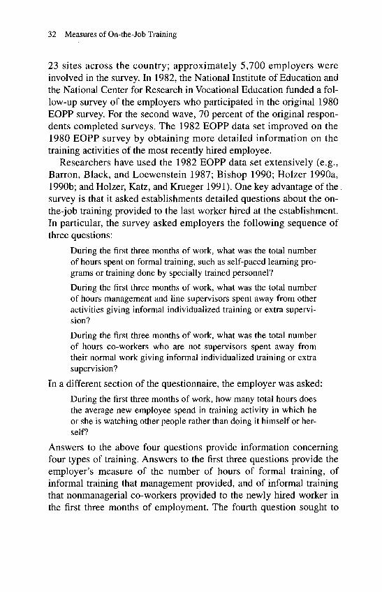
23 sites across the country; approximately 5,700 employers were involved in the survey. In 1982, the National Institute of Education and the National Center for Research in Vocational Education funded a fol low-up survey of the employers who participated in the original 1980 EOPP survey. For the second wave, 70 percent of the original respon dents completed surveys. The 1982 EOPP data set improved on the 1980 EOPP survey by obtaining more detailed information on the training activities of the most recently hired employee.
Researchers have used the 1982 EOPP data set extensively (e.g., Barren, Black, and Loewenstein 1987; Bishop 1990; Holzer 1990a, 1990b; and Holzer, Katz, and Krueger 1991). One key advantage of the survey is that it asked establishments detailed questions about the on- the-job training provided to the last worker hired at the establishment. In particular, the survey asked employers the following sequence of three questions:
During the first three months of work, what was the total number of hours spent on formal training, such as self-paced learning pro grams or training done by specially trained personnel?
During the first three months of work, what was the total number of hours management and line supervisors spent away from other activities giving informal individualized training or extra supervi sion?
During the first three months of work, what was the total number of hours co-workers who are not supervisors spent away from their normal work giving informal individualized training or extra supervision?
In a different section of the questionnaire, the employer was asked:
During the first three months of work, how many total hours does the average new employee spend in training activity in which he or she is watching other people rather than doing it himself or her self?
Answers to the above four questions provide information concerning four types of training. Answers to the first three questions provide the employer©s measure of the number of hours of formal training, of informal training that management provided, and of informal training that nonmanagerial co-workers provided to the newly hired worker in the first three months of employment. The fourth question sought to
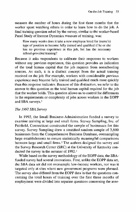
On-the-Job Training 33
measure the number of hours during the first three months that the worker spent watching others in order to learn how to do the job. A final training question asked by the survey, similar to the worker-based Panel Study of Income Dynamics measure of training, was:
How many weeks does it take a new employee hired for (name©s) type of position to become fully trained and qualified if he or she has no previous experience in this job, but has the necessary school-provided training?
Because it asks respondents to calibrate their responses to workers without any previous experience, this question provides an indication of the total human capital that the job requires from nonschooling sources. As such, it is a distinct concept from the actual training received on the job. For example, workers with considerable previous experience may become fully trained and qualified much more quickly than this response indicates. Because of this distinction, we refer to the answer to this question as the total human capital required for the job that the worker holds. This question allows us to control for differences in the requirements or complexity of jobs across workers in the EOPP and SBA surveys. 1
The 1992 SBA Survey
In 1992, the Small Business Administration funded a survey to examine training at large and small firms. Survey Sampling, Inc. of Fairfield, Connecticut constructed the sample of businesses for this survey. Survey Sampling drew a stratified random sample of 3,600 businesses from the Comprehensive Business Database, oversampling large establishments to ensure statistically meaningful comparisons between large and small firms. 2 The authors designed the survey and the Survey Research Center (SRC) at the University of Kentucky con ducted the survey in the summer of 1992. 3
While based on the survey methodology of the EOPP data, the SBA- funded survey had several innovations. First, unlike the EOPP data set, the SBA data set did not oversample low-income workers, nor was it targeted only at sites where new government programs were planned. The survey also differed from the EOPP data in that the questions con cerning the total hours of training over the first three months of employment were divided into separate questions concerning the aver-

34 Measures of On-the-Job Training
age number of hours of training per week and the number of weeks of training. This approach allowed us to discover to what extent training was complete by the end of the first three months of employment. Finally, in addition to the EOPP©s four measures of training (formal training programs offered by the firm on site, informal training by the worker©s supervisor, informal training by co-workers, and time that the worker spent watching others perform tasks during the first three months), the SBA survey added a fifth measure, the number of hours spent at off-site formal training programs during the first three months of employment.
To check how the set of completed SBA surveys compares to the ini tial stratified national sample, we estimated a probit equation with the dependent variable equal to one if the establishment was in the sample, and zero otherwise. For independent variables, we used a set of one- digit industry dummies, Census region, a dummy variable indicating whether the establishment was located in a Metropolitan Statistical Area, and a vector of establishment-size variables. 4 Establishments from SIC code 7 (a portion of the service industry [10.2 percent in sample versus 16.6 percent universe]) and SIC code 5 (retail trade [30.8 percent versus 33.0 percent]) are somewhat underrepresented in our sample. Similarly, there are too few establishments from the North east Census region (13.7 percent versus 17.4 percent), and there are too few urban establishments (77.6 percent versus 85.1 percent). In addi tion, the probability of inclusion in our sample monotonically increases with the size of the establishment. However, the differences are not large, and one can conclude that the sample of firms that completed the survey is generally representative of the underlying national population of firms.
Employer Measures of On-the-job Training
Table 3.1 reports the magnitude and incidence of training for the two surveys. Figure 3.1 illustrates the differences in the means of the various measures of training between the EOPP and SBA data sets. Note that the overall means are quite similar. For the EOPP data, newly hired workers receive about 142 hours of training in the first three

On-the-Job Training 35
months, with about 95 percent of all workers receiving some form of training; for the SBA data, newly hired workers receive about 150 hours of training with 98 percent of all workers receiving some train ing.5 For the individual training measures, the off-site formal training (which is unique to the SBA) is a relatively minor form of training; average newly hired workers receive about three hours of this training while only about 7 percent of all workers receive this form of training. Thus, if we subtract the three hours of off-site formal training from the SBA mean, the two data sets indicate a remarkable degree of similarity.
Table 3.1 Means and Incidence Rates of Training Measures, 1992 SBA Data and 1982 EOPP Data
Total hours of training
Incidence rate
Hours of off-site formal training
Incidence rate
Hours of on-site formal training
Incidence rate
Hours of informal management training
Incidence rate
Hours of informal co-worker training
Incidence rate
Hours of watching others
Incidence rate
N
SBA
149.9
0.978
3.4
0.069
13.6
0.205
59.4
0.906
32.8
0.605
40.7
0.645
1,123
EOPP
141.9
0.948
11.9
0.151
49.3
0.872
26.3
0.628
54.5
0.803
1,916
Within specific categories of training, table 3.1 reveals some differ ences in the average level and incidence of training. For instance, inci dence of formal training is higher in the SBA data than in the EOPP data. In contrast, the EOPP reports more training by watching others than does the SBA data. For the EOPP, the newly hired worker has an average of about 54 hours with an incidence rate of 80 percent, but for

36 Measures of On-the-Job Training
the SB A data, the average number of hours is only about 41 hours with an incidence rate of 65 percent.
Figure 3.1 EOPP and SBA Measures of Average Hours Spent in On-the-job Training During First Three Months
150
120
90
X 60
30
SBA EOPP
Total hours Hours of Hours of Hours of Hours ofof training on-site formal informal informal watching
training management co-worker otherstraining training
A comparison of means and incidence rates, however, can be some what deceiving. The length of training in the first three months can be a very skewed variable, and the mean is somewhat sensitive to large observations in the right tail of the distribution. Therefore, in table 3.2, we provide the mean, and the 5th, 10th, 25th, 50th, 75th, 90th, and 95th percentiles for each training measure conditional on the measure being positive. In each case, the mean of the distribution is considerably larger than the median of the distribution, indicating that the distribu tions are skewed to the right.
A weakness of both the EOPP and SBA data is their reliance on training received in the first three months of employment. We have just seen the importance of the right-hand tails of the data in generating dif ferences in unconditional means in training between the SBA and EOPP data. To understand the significance of the three-month trunca tion of training, table 3.3 lists, for each type of training, the probability that a training spell lasts at least 12 weeks (both the unconditional

Table 3.2 Comparison of 1992 SBA and 1982 EOPP Training Measures
Formal Training
Percentile
5th
10th
25th
50th
75th
90th
95th
Mean
N
SBAOff-site
4
4
16
30
40
120
240
48.1
110
SBAOn- site
4
6
16
35
80
180
240
66.9
318
EOPPOn-site
4
6
16
40
100
200
240
78.6
252
SBAManagement
1
4
12
30
65
160
240
65.5
1,012
EOPPManagement
2
4
10
30
70
120
200
56.6
1,645
Informal Training
SBACo-worker
2
3
10
21
60
120
240
54.2
766
EOPPCo-worker
2
4
8
20
48
100
145
41.8
1,157
SBA
Watching others
2
4
8
24
65
160
360
63.1
765
EOPP
Watching others
3
5
10
32
80
160
240
67.9
1,512

38 Measures of On-the-Job Training
probabilities and the more revealing probabilities conditional on receiving the type of training) for only the SBA data. We cannot con struct a similar table for the EOPP data because that set only contains information on the total number of hours, not length, of training. We choose 12 weeks because both 12 and 13 weeks are mass points. While a three-month period contains 13 weeks, we thought many respondents believed that period to contain 12 weeks. We refer to an incidence of training that lasts at least 12 weeks as a truncated incidence, although it is possible that the incidence would end exactly on the 12th week. From table 3.3, we see that 29 percent of training spells are truncated at three months. Conditional on receiving each type of training, the trun cation rates are very high, with each measure having more than one in five cases truncated. Thus, the three-month frame of reference used by both the SBA and EOPP data appears to understate the training that newly trained workers received.
Table 3.3 Rates of Training Spells Lasting at Least 12 Weeks, 1992 SBA Data
Training measure
Total training
Off-site training
On-site training
Informal management training
Informal co- worker training
Watching others
Overall rate
0.291
0.016
0.042
0.217
0.157
0.146
Conditional rate
0.298
0.230
0.204
0.239
0.259
0.226
Finally, in table 3.4 we compare the reported time it takes to become fully trained and qualified. For the EOPP data, this measure of total human capital has a mean of 20.2 weeks, but the median is only 6.75 weeks. The SBA data set reveals a similar mean for total human capital of 22.2 weeks but a median of just 6 weeks. Again, both measures are highly skewed to the right. In sum, the two distributions of total human capital look very similar despite the ten-year difference in the time periods.

On-the-Job Training 39
Another issue that could cloud comparisons between the 1982 EOPP data and the 1992 SBA data is the effect of the business cycle on training. The EOPP survey was conducted in the first half of 1982 just prior to the trough of the cycle in November 1982. The SBA survey was conducted in the summer of 1992, just over a year past the trough of the cycle in March 1991. The training data for the last worker hired precedes the date of the survey by at least 3 months by construction. Thus, much of the EOPP training data precedes the 1982 trough of the cycle by several months, and much of the SBA data is very close to the 1991 trough. It could be that training decisions of firms are different at the trough of the cycle from those before or after it. If so, comparisons made between the SBA and EOPP data could be affected. Unfortu nately, the EOPP and SBA cannot be used to provide evidence on this question. However, tabulations by James Spletzer using the National Longitudinal Survey of Youth (NLSY) provide evidence on the inci dence of formal training over the cycle that had its trough in 1991. Spletzer finds that the incidence of training is the lowest in 1991 at the trough of the cycle. Using a probit model, the probability of receiving training in 1990, one year before the trough, is only slightly higher. 6 This suggests that any contamination from business cycle effects is likely to be small when comparing the EOPP and SBA data.
Table 3.4 Length of Time to Become Fully Trained and Qualified, 1992 SBA Data and 1982 EOPP Data
Percentile
5th
10th
25th
50th
75th
90th
95th
Unconditional mean
Fraction nonzero
N
SBA
.55
1
2.25
6
24
52
104
22.2
.991
1,193
EOPP
1
1
2.8
6.75
22.1
52
94
20.2
0.969
1,921

40 Measures of On-the-Job Training
In other words, the EOPP and SBA were both conducted close enough to the trough of a business cycle to avoid any contamination from business cycle effects. However, comparisons between the EOPP, SBA and surveys conducted further into an expansion or at the peak of the cycle may be affected. The Spletzer results run counter to the argu ment that as firms stockpile their most capable workers during a down turn, they increase their training activities. Of course, Spletzer©s results are for the incidence of training and suggest that firms do not train more extensively during economic downturns, but they may train some workers more intensively. However, if his results hold for the provision of training in general, then the EOPP and SBA surveys would under- predict the incidence of training at other points in the business cycle.
Overall, the 1982 EOPP data and the 1992 SBA data give very simi lar answers on the provision of training. In some respects, these simi larities of the data sets surprised us. The 1980s was a decade of fundamental change in the distribution of wages in the U. S. economy. 7 During that time, the distribution of wages became much more dis persed, and little overall growth in real wages occurred. For some groups in particular, those below the median earnings of the econ omy there was a decline in real wages. For others, especially workers in the upper quintile of the earnings distribution, there was a substan tial increase in real wages for high-wage workers. Given the apparent importance of on-the-job training in wage determination, one may have anticipated a similar increase in the dispersion of on-the-job train ing. Comparing these two data sources, however, we find only limited evidence of such an increase in the dispersion of on-the-job training. The SBA data appear to have a somewhat greater dispersion for man agement training and co-worker training, and have a somewhat greater incidence of formal training than the EOPP data, although the differ ences are not substantial. One must bear in mind, however, that both data sets are truncated at the first three months of employment and may hide some important changes in the distribution of on-the-job training. Further, the sample for the EOPP data is not nationally representative.

On-the-Job Training 41
Worker Measures of On-the-job Training
Another approach to measuring on-the-job training asks employees about their training experiences. Obviously, most data will not have a collection of newly hired workers, so worker surveys will include a considerable number of workers with a significant amount of tenure. If these workers receive less training than newly hired workers, and if workers are asked about their training activities over a relatively short period of time, very low incidence rates for training are likely to occur. As a result, surveys of workers tend to ask very general training ques tions; however, one still finds very low incidence rates of training from worker surveys.
The first commonly used data on training was the Panel Study of Income Dynamics (PSID), which in 1976 asked a question similar to the EOPP and SBA question about the time to become fully trained and qualified. The PSID asked:
On a job like yours, how long would it take the average new per son to become fully trained and qualified?
Duncan and Hoffman (1978, 1979) were the first to analyze these data; they note that the instrument used the phrase "the average new person" rather than "you" in order to "minimize reported training differences due to skills or experience unique to the respondent" (1979, p. 596).
This wording, however, creates a potential difference between the frames of reference of the PSID data and the EOPP and SBA data. Namely, the PSID does not explicitly tell the respondent to assume that the new person has no previous experience, while both the EOPP and SBA do explicitly ask the respondent to make this assumption. 8 Keep ing this potential difference in mind, Duncan and Hoffman report that the mean response to this question was 1.66 years, or about 86.32 weeks. The PSID sample, however, contains many individuals with a great deal of tenure at their employers. Black, Garen, and Loewenstein (1988) report that there is a very strong concave relationship between tenure at the firm and the length of time to become fully trained and qualified; therefore, we should not be surprised that the PSID mean is so much larger than the EOPP and SBA means.
The National Longitudinal Survey of the High School Class of 1972 (NLSHS72) provides a more detailed set of questions concerning train-

42 Measures of On-the-Job Training
ing. Altonji and Spletzer (1991) provide an excellent description and analysis of these data. In 1986, the survey asked for the number of weeks and the number of hours per week of four different forms of training in the worker©s current job or last job held by the worker. These forms of training included employer-provided formal training (which Altonji and Spletzer suggest corresponds to the SBA on-site formal training), informal training, off-site training, and any tuition or financial aid that the employer offered to employees attending an edu cational institution. The sample of workers is limited to individuals who graduated from high school. The training questions ask about any training received at any time on the last job, and some workers may have considerable tenure at the job.
Altonji and Spletzer report that 45.7 percent of workers receive some employer provided training that is, some formal, informal, or off-site training. For the individual training measures, 27.8 percent of all workers report that they received formal on-site training. This figure is somewhat higher than the 20.4 percent reported in the SBA data and the 15.1 percent reported by the EOPP data. The mean hours of formal training is 52.7 hours, but unlike the SBA and EOPP data, the NLSHS72 data is truncated at 93 weeks of training, so the means are not directly comparable. The mean duration of formal training, condi tional on receiving this type of training, is 10.9 weeks, and more than a quarter of the sample has a duration lasting 12 weeks or longer, which is somewhat higher than the SBA figure of 20.4 percent. Given that these workers are more educated than workers in the two other data sets and given also that many of them have considerable tenure on the job, these differences do not appear to be overly large.
The informal training, however, has a much lower incidence (19.7 percent) than the other two data sets. In contrast, the incidence rates of informal training by management in both the EOPP and the SBA data are more than 85 percent. Thus, it would appear that the incidence of informal training is underreported in the NLSHS72 data. In our view, this finding is not particularly surprising. Formal training is probably much easier to remember than informal training, especially after sev eral years have elapsed. Moreover, the worker may not recognize as "real" training much of the informal training that occurs. A newly hired worker may not consider asking a co-worker for assistance or some advice to be training, but the employer may count this as training,

On-the-Job Training 43
especially if it detracts from the performance of the co-workers. The mean number of hours of this type of training is 45.8 hours. The mean conditional on receiving informal training, however, is 233 hours, and half the sample reports the training lasting at least 20 weeks. To us, this seems to indicate that workers are more likely to remember the very long spells of informal training. As SBA data indicates that most spells of informal training last less than 12 weeks, this may account for the relatively low incidence rate of informal training in the NLSHS72 data.
Another large difference between the NLSHS72 and the SBA data lies in the incidence rate of off-site training. For the NLSHS72, Altonji and Spletzer report an incidence rate of 20.0 percent, whereas the SBA data indicates only a 6.9 percent incidence rate. While some of this dif ference may be explained by variances in the education levels of the two samples, the disagreement is still too large. Off-site training often involves a considerable expense because it may involve substantial direct costs in fees or tuition, and because it may be necessary to send the worker to a different location for training, incurring transportation, food, and lodging expenses. Firms and workers may wish to ensure a beneficial employment match before incurring such costs. Thus, we might anticipate that the off-site training incidence is somewhat higher for more senior workers because the likelihood of a separation declines with the worker©s tenure. The mean hours of training, conditional on receiving this type of training, is 101.3 hours, which is considerably larger than the SBA©s conditional mean of 48 hours.
Finally, Altonji and Spletzer note that the incidence of a worker tak ing advantage of tuition plans is 9.4 percent, with a mean of 18.2 hours. The mean conditional on an incidence of this type of training is 193 hours with a mean duration of 27 weeks. This suggests that formal schooling continues to be a rather important part of the training pro grams of many firms. Loewenstein and Spletzer (1993) report a similar rate for the CPS data (13.6 percent).
A comparison of the incidence rates and hours of training measures from the NLSHS72, EOPP, and SBA data provides four interesting observations. First, there is somewhat more formal training among workers as a whole than among a sample of newly hired workers. Sec ond, this difference for off-site formal training is even more pro nounced than for on-site formal training. These two observations suggest that formal training is more prevalent for workers with some

44 Measures of On-the-Job Training
tenure than for newly hired workers. Third, there are many incidences of on-site formal training and informal training that last longer than 12 weeks, which suggests that the EOPP and the SBA three-month frame may understate the training that newly hired workers received. Fourth, employees seem to understate the incidence of informal training, with workers more likely to remember particularly long spells of informal training. Given the prevalence of informal training that we find in the EOPP and SBA data, this suggests that relying on surveys of workers will lead to an understatement of the importance of informal on-the-job training.
To examine further the differences in formal training programs, we consider the National Longitudinal Survey of Youth, which is a survey of over 12,500 youths ranging in age from 14 to 22 years in 1979. Lynch (1992), Veum (1993), and Bartel and Sicherman (1993) provide analysis of this data set for different time periods. Concentrating on data from 1979 to 1985, Lynch focuses on a sample of workers who did not complete college and who received formal on-the-job training lasting at least four weeks. These limitations result in a sample of 3,064 workers. The four-week length of a training spell is a sampling feature of the early NLSY training measures. Lynch reports that only 4.2 percent of the workers in her sample had this type of on-the-job training, but that the average length of this type of training was 31 weeks. In contrast, in the SBA data 38 percent of all training inci dences lasted at least four weeks so the incidence rate of formal train ing programs lasting at least four weeks is about 7.8 percent (20.5 percent of all workers receive any on-site formal training and 38.0 per cent of these incidences last at least four weeks). Given that Lynch excludes college graduates from her sample and that, as we shall later see, college graduates are more likely to receive formal training pro grams, these two incidence rates appear very similar. This suggests that her conditional mean for formal training spells is a reasonable estimate of the conditional mean, although it is a bit low because it excludes college graduates. Lynch©s results suggest that the distribution of time in formal on-the-job training spells has extremely thin but very long tails. By focusing on the training received in the first three months, sur veys such as the SBA survey and the EOPP survey cut off that long tail, which may cause researchers to underestimate the training that newly hired workers receive.
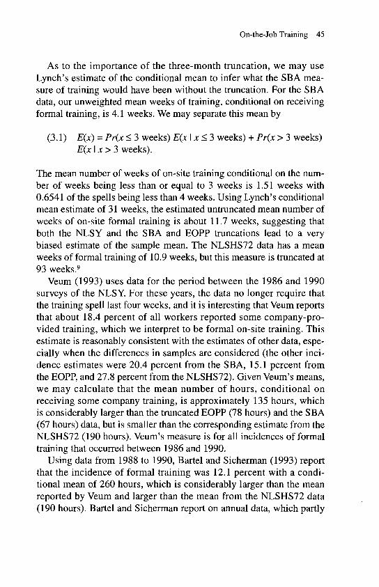
On-the-Job Training 45
As to the importance of the three-month truncation, we may use Lynch©s estimate of the conditional mean to infer what the SBA mea sure of training would have been without the truncation. For the SBA data, our unweighted mean weeks of training, conditional on receiving formal training, is 4.1 weeks. We may separate this mean by
(.3.1) E(x) = Pr(x < 3 weeks) E(x I x < 3 weeks) + Pr(x > 3 weeks) E(x \x>3 weeks).
The mean number of weeks of on-site training conditional on the num ber of weeks being less than or equal to 3 weeks is 1.51 weeks with 0.6541 of the spells being less than 4 weeks. Using Lynch©s conditional mean estimate of 31 weeks, the estimated untruncated mean number of weeks of on-site formal training is about 11.7 weeks, suggesting that both the NLSY and the SBA and EOPP truncations lead to a very biased estimate of the sample mean. The NLSHS72 data has a mean weeks of formal training of 10.9 weeks, but this measure is truncated at 93 weeks.9
Veum (1993) uses data for the period between the 1986 and 1990 surveys of the NLSY. For these years, the data no longer require that the training spell last four weeks, and it is interesting that Veum reports that about 18.4 percent of all workers reported some company-pro vided training, which we interpret to be formal on-site training. This estimate is reasonably consistent with the estimates of other data, espe cially when the differences in samples are considered (the other inci dence estimates were 20.4 percent from the SBA, 15.1 percent from the EOPP, and 27.8 percent from the NLSHS72). Given Veum©s means, we may calculate that the mean number of hours, conditional on receiving some company training, is approximately 135 hours, which is considerably larger than the truncated EOPP (78 hours) and the SBA (67 hours) data, but is smaller than the corresponding estimate from the NLSHS72 (190 hours). Veum©s measure is for all incidences of formal training that occurred between 1986 and 1990.
Using data from 1988 to 1990, Bartel and Sicherman (1993) report that the incidence of formal training was 12.1 percent with a condi tional mean of 260 hours, which is considerably larger than the mean reported by Veum and larger than the mean from the NLSHS72 data (190 hours). Bartel and Sicherman report on annual data, which partly

46 Measures of On-the-Job Training
explains their lower incidence rates for the total training received over a four-year period. We are still unclear why Veum©s estimates of the hours trained are so much smaller than Bartel and Sicherman©s esti mates.
The Current Population Survey (CPS) provides cross-sectional esti mates of the incidence of training that workers received before or on their current job both in 1983 and 1991. Lillard and Tan (1992) and Pergamit and Shack-Marquez (1987) analyze the 1983 data. The CPS on-the-job training data may be divided into formal and informal train ing programs. Lillard and Tan report that 11.7 percent of men needed formal (what they call "company") training on their previous job to obtain their current job, and 11.6 percent of men needed formal train ing while on their current job. If we combine those two estimates, we obtain an incidence rate of approximately 23 percent, although clearly we may have some double counting. Pergamit and Shack-Marquez (1987) report that 30 percent of their sample, which differs from Lil lard and Tan©s sample, received training both before and during their current jobs. Thus, a back-of-the-envelope calculation to correct for the double counting suggests an incidence rate of about 20 percent. For women, the sum of the two training measures was 20.6 percent and fell to 18 percent when we corrected for double counting.
If one takes the more conservative estimates of training on the cur rent job 13.1 percent for women and 11.6 percent for men we do see a lower incidence rate than data from the other samples. It is impor tant to keep in mind, however, that the CPS sample is representative of all workers in the economy. Previous data sets discussed thus far have not sampled all workers, and this variation may account for some of the differences in the data sets. Most important, unlike the EOPP and SBA data, the CPS is not a sample of newly hired workers, who receive most of the training among all workers. Using a different CPS sample, Pergamit and Shack-Marquez report that the incidence rate of formal training on the current job is 14.2 percent.
For informal on-the-job training, Lillard and Tan report that 15.1 percent of men and women received informal training on their current job, and 30.8 percent of the men and 26.0 percent of the women said they received training on their previous job that was necessary to obtain their current job. Thus, the incidence rates from the CPS are well below the incidence rates of the SBA and EOPP data. This again

On-the-Job Training 47
may reflect the fact that workers are less likely to remember incidences of informal training.
Loewenstein and Spletzer (1993), using the 1991 CPS data, also report an extremely low incidence rate of informal training 16.3 per cent. While this figure is somewhat higher than the 1983 CPS esti mates, it is much lower than the employer-reported estimates from the SBA and the EOPP data. Indeed, the estimate is quite similar to the 19.7 percent figure Altonji and Spletzer (1991) obtained from the NLSHS72. Therefore, the CPS data also seem to suggest that workers may underreport the incidence rate of informal training.
In contrast, Loewenstein and Spletzer report an incidence of 17.2 percent for formal training, which is reasonably similar to the employer-reported incidence rates in the EOPP and SBA data (15.1 percent and 20.5 percent, respectively), and the employee-reported incidence rates from the NLSY and NLSHS72 (12.1 percent to 18.4 percent and 27.8 percent, respectively). While the 1983 CPS data gives somewhat lower incidence rates, and the NLSHS72 shows slightly higher incidence rates, employee- and employer-reported incidence rates appear reasonably similar for formal training. Moreover, compar ing the 1982 EOPP survey and 1992 SBA survey of employers, and comparing the 1983 CPS and the 1991 CPS of employees, there is some modest evidence of an increase in formal training. For the employer surveys, training increased from 15 to 20 percent, and for the employee surveys, training increased from 12 to 17 percent. 10
The 1991 CPS data also reported the duration of the training that the worker received. Loewenstein and Spletzer report that the mean dura tion of formal training, conditional on receiving formal training, is 9.6 weeks. This estimate approximates the NLSHS72 estimate of 10.9 weeks and the SBA estimate (adjusted for the truncation using Lynch©s conditional mean) of 11.7 weeks. Thus, measures of the duration and the incidence rates of formal training appear similar.
Finally, the Survey of Income and Program Participation (SIPP) in 1984 provides another data source to measure training. But because the incidence rates are extremely small, we are suspicious of the data. Flynn (1993) and Haber (1988) report that the SIPP survey asked in 1984, "did [you] receive training designed to help [you] find a job, improve job skills or learn a new job?" Although this appears to be a very broad question encompassing formal and informal job training as

48 Measures of On-the-Job Training
well as vocational and technical schooling, Haber estimates that only 23 percent of workers in his sample had ever received any training, and only 9.4 percent of all workers had ever received on-the-job training. In our view, these estimates are much too low and indicate that the SIPP data missed a great deal of training.
Conclusions
We conclude with the following five observations concerning employee- and employer-reported measures of training.
1. Employee- and employer-based data sets appear to provide simi lar estimates of the incidence of on-site formal training, and there is at least some evidence that the measures of the duration of training estimates are not dissimilar.
2. The EOPP and SBA data, which measure training only for the first three months of employment, appear to understate training substantially. Evidence from the SBA and NLSHS72 studies sug gests that the difference matters for both formal and informal training. Similarly, the early NLSY estimate that only measures formal training programs of at least four weeks in length also appears to miss a great deal of the formal training.
3. A comparison of the SBA and NLSHS72 data suggests that the incidence of off-site training may increase with the worker©s ten ure.
4. Comparing the EOPP and SBA data with the PSID data, there is some evidence that employees may understate (relative to employers) the length of time to become fully trained and quali fied.
5. The incidence rates for informal training reported by employees are dramatically below the incidence rates for informal training reported by employers.
There is one caveat: Our examination of the means of various train ing measures from different surveys may not provide a good indication

On-the-Job Training 49
of how precisely we are measuring training. Even if employees and employers provide estimates of training that have identical means, there may be considerable measurement error in the reports of both employers and employees. If the measurement error is completely ran dom, the means may be quite similar, but the training measures them selves are very inaccurate.
NOTES
1. Part of these differences may also reflect the fact that the skills required of more complex jobs are more complementary with physical capital such as computers or with high-performance workplace transformations.
2. The sample was stratified by establishment size in the following manner: 1,250 establish ments with 0-19 employees, 1,250 establishments with 20-99 employees, 550 establishments with 100-499 employees, and 550 establishments with 500 or more employees. We excluded Agricul ture, Forestry, and Fisheries (SIC 0-99) and Public Administration (SIC 900 and above). Except for these exclusions, we sampled establishments randomly within each size stratum, providing a representative distribution by industry and region.
3. We first sent a letter to each establishment describing the survey. SRC attempted to track down establishments with undeliverable letters using directory assistance and attempted to contact each of the 3,600 establishments for a telephone interview. Of the original sample of 3,600 estab lishments, 2,561 were eligible to complete an interview. The 1,039 ineligible establishments were out of business, had disconnected phones, did not answer in any of 15 attempts, could not be reached because of Hurricane Andrew, had other miscellaneous problems, or had no employees. We had 1,288 establishments complete the survey. The 1,273 noncompletions consisted of refus als, those who reported that answering surveys was against company policy, those who stated that the appropriate person was repeatedly unavailable, and those who rescheduled the interview six or more times.
4. The breakdowns for firm size were 1-4 employees, 5-9 employees, 10-19 employees, 20-49 employees, 50-99 employees, 100-199 employees, 200-499 employees, and 500 or more employ ees.
5. To enhance comparability of the samples, EOPP and SBA sample weights are used in the training computations reported in this chapter. The SBA weights account for the stratification by establishment size and the oversampling of large firms. The EOPP weights account for the over- sampling of smaller, single establishments firms within each target metropolitan area.
6. Relative to the reference year of 1993, the 1991 coefficient is -.0303 (t = 4.53) and the 1990 coefficient is -.0306 (t = 4.44). We thank James Spletzer for kindly providing these estimates.
7. See Juhn, Murphy, and Pierce (1993) or the special issues of the Quarterly Journal of Eco nomics (February 1992) for references.
8. See Sicherman (1990) for a discussion of this point and related issues concerning the PSID training measure.
9. The reader should keep in mind, of course, that combining these two estimates makes heroic distributional assumptions, but we believe that it does indicate a very important limitation of both data sets. The NLSY misses a majority of the spells of formal training, and the SBA and EOPP data truncate the very long spells of training that are an important determinant of total training.

50 Measures of On-the-Job Training
10. In a remarkably thorough study of all forms of training, Lillard and Tan (1992) also report incidence rates from the National Longitudinal Surveys of young men and mature men, which were conducted in various years ranging from 1967 to 1982. They report that the incidence of for mal training in a two-year period for young men is 10.4 percent and for mature men, 5.6 percent. It is difficult, however, to directly compare these data with either the CPS or employer-provided data.

CHAPTER
Who Receives On-the-Job Training?
With the development of data sets containing explicit measures of on-the-job training, economists have been able to identify the recipi ents of on-the-job training. Because of the importance of on-the-job training in determining wages, this question is of considerable interest. According to traditional on-the-job training models developed in chap ter 2, workers with jobs that offer little or no training should not antici pate large increases in wages, since work experience does little to increase their stock of human capital. If workers with different per sonal characteristics differ in their access to on-the-job training, wage differences across workers may be attributed, in part, to these differ ences in access.
This chapter examines the recipients of on-the-job training from the perspective of two employer-reported data sets: the 1982 Employment Opportunity Pilot Project (EOPP) survey and the 1992 Small Business Administration (SBA) survey. Both data sets contain two types of training measures. The first measure is the actual number of hours of training that newly hired workers received in the first three months of employment. The second measure, one that indicates the total human capital of a particular job, is the length of time it would take the worker to become fully trained and qualified if that worker had no previous experience on the job. While these data are limited to newly hired workers, evidence presented in chapter 3 suggests that many current data sets that rely on employee reports of training appear to exclude significant amounts of on-the-job training. In contrast, the SBA and EOPP surveys offer us a reasonably detailed account of the training that newly hired workers received at two points in time that are ten years apart.
51

52 Who Receives On-the-Job Training?
Variations in the Level of Training
In approaching the issue of which employees have access to on-the- job training, we proceed in stages. In the first part of this section, we consider the simple gross differences in various levels of training by workers who differ in their level of education, work experience, size of employer, and gender. The second part of this section provides a more comprehensive examination of who has access to training. The results presented there establish the statistically significant links between vari ous characteristics of individuals and their level of training, with other factors being equal. The next section examines the incidence of five types of training: off- site formal training, on-site formal training, informal management training, informal co-worker training, and train ing by watching others. To understand the importance of the truncation of our training measure at the first three months of employment, the final section of this chapter examines the likelihood that each type of training may continue after the first three months.
Differences by Education, Experience, Gender, and Employer Size
Not surprisingly, we find that those characteristics that are highly correlated with wages are also correlated with access to on-the-job training. For instance, in both the 1982 EOPP and the 1992 SB A data sets, we find that highly educated workers receive more on-the-job training. In figure 4.1, we depict the mean level of training for college and high school graduates from the SBA data. College graduates receive over one hundred more hours of on-the-job training in the first three months of employment than do high school graduates, or nearly 68 percent more training. Thus, employers of more educated workers provide them with more on-the-job training.
Figure 4.1 Hours of Training in the First Three Months of Employment, 1992 SBA Data
Cdlegegrcducte Hlg^scrioolgxrlucte;
50 100 160 200 250 300
Hours

On-the-Job Training 53
The difference between college and high school graduates is even more dramatic when we look at the time required to become fully trained and qualified. In figure 4.2, we depict the means for the time to become fully trained for college and high school graduates. On the average, college graduates occupy jobs that required about 95 percent more time to become fully trained, with college graduates taking nearly 37 weeks to become fully trained and high school graduates only 19 weeks.
Figure 4.2 Number of Weeks to Become Fully Trained and Qualified, 1992 SBA Data
College grducte" Hl^i school g-cducte
35 40Weeks
Thus, college graduates obtain jobs that are more complex and pro vide more on-the-job training than do those with only a high school education.
Another important determinant of wages is a worker©s labor market experience. In figure 4.3, we depict the average training received by workers with three levels of experience: those with no previous experi ence, those with less than a year of experience, and those with more than a year of experience. Workers with no previous experience received the lowest level of training, only about 164 hours. In contrast, workers with less than a year of experience received nearly 198 hours of training. Workers with more than a year of experience received only about 178 hours of training. These figures suggest that workers with significant experience may require less training because some of the skills that these workers learn at one employer can be transferred to their new jobs.
The relationship between labor market experience and the time to become fully trained and qualified seems to confirm the suggestion that skills are transferable across jobs. In figure 4.4, we depict the means of time to become fully trained by level of experience. Unlike hours of training, the total human capital required for a job increases as the

54 Who Receives On-the-Job Training?
worker develops more experience. In other words, workers with more experience are hired into more complex jobs that require more total human capital. For workers without any experience, it takes just over 16 weeks to become fully trained, but for a worker with less than a year of experience, the training takes just over 23 weeks. Workers with more than a year of experience occupy jobs that require nearly 29 weeks to become fully trained. Thus, firms tend to hire workers with more experience to fill complex jobs. But as a result of their experience in previous jobs, these workers may require less training than workers filling jobs that require less total human capital.
Figure 4.3 Hours of Training in the First Three Months of Employment by Experience Level, 1992 SBA Data
Morelhcnayeaof experience
Lesslhcnayeaof experience
No experience^^^^^^^^^^™
80 100 120 140 160 180 200
Hours
Figure 4.4 Time to Become Fully Trained and Qualified by Experience Level, 1992 SBA Data
More than a year ofexperience
Less man a year ofexperience
No experience
Labor economists have also found that workers employed in large establishments tend to receive higher wages than similar workers in small establishments (e.g., Barron, Black, and Loewenstein 1987; Holtmann and Idson 1991). Similarly, both the EOPP and SBA data indicate that workers in large establishments receive more training than workers in small establishments. In figure 4.5, for the SBA data we

On-the-Job Training 55
depict the mean hours of training by four categories for the size of establishment: those establishments with less than 25 employees, those with 25 to 99 employees, those with 100 to 249 employees, and those with 250 or more employees. Workers in establishments with fewer than 25 employees received about 154 hours of training in the first three months of employment, while workers in establishments with 250 or more employees received over 220 hours of training. Thus, workers in the largest category of establishments received 42 percent more training than workers in the smallest category. Interestingly, nei ther the EOPP nor the SBA data reveal any significant difference in the time to become fully trained by size of establishment. Of course, larger establishments are training their workforces more intensively in the first three months than smaller establishments, so these large employ ers presumably are providing their workforces a greater stock of human capital.
Figure 4.5 Hours of Training in the First Three Months of Employment by Establishment Size, 1992 SBA Data
250 or more employees
100 to 249 employees
25 to 99 employees
Fewer than 25 employees
Hours
There remain very significant racial and gender differences in the wage structure across the United States economy, and one might antic ipate that there would exist very substantial differences in the access to on-the-job training as well. Surprisingly, both the EOPP and SBA data provide little evidence that women receive significantly fewer hours of training in the first three months of employment than men. Unfortu nately, the EOPP data contain no controls for the employee©s race, but the SBA data do not indicate significant racial differences in hours of training in the first three months. In contrast, figure 4.6 shows that there are significant racial and gender differences in the time to become fully trained and qualified. Blacks occupy jobs that take about

56 Who Receives On-the-Job Training?
9 weeks to become fully trained and qualified, nonblack women occupy jobs that take about 17 weeks to become fully trained, and non- black men occupy jobs that take over 35 weeks to become fully trained and qualified. Given these differences, it is surprising that we find no significant differences in the hours of training in the first three months of employment, although we do find some evidence that limiting train ing to the first three months of employment might be partially respon sible for not finding any gender differences. Because our measures of training are limited to the first three months, it is possible that men will obtain more total training if they are more likely than women to have training last beyond our three-month horizon.
Figure 4.6 Time to Become Fully Trained and Qualified by Race and Gender, 1992 SBA Data
Worker is beck
Statistical Patterns Regarding Access to On-the-Job Training
The differences in training identified above still appear when we control for other factors with the use of regression analysis. In what follows, we analyze variations in on-the-job training in a more system atic fashion. For both the EOPP and the SBA data, we begin by esti mating the total hours of training in the first three months of employment. For the EOPP data, the training measure is the sum of formal training, informal management training, co-worker training, and watching others. For the SBA data, we use the same four catego ries, and we add the number of hours of off-site training, although the results change little if we exclude this measure.
For independent variables in the SBA data, we use the worker©s age, a vector of dummy variables indicating whether or not the worker is a high school dropout, whether or not the worker attended but did not graduate from college, and whether or not the worker has at least a

On-the-Job Training 57
four-year college degree. In both the EOPP and SBA surveys, employ ers were asked the number of years of labor market experience that an employee had in a job that the employer felt "had some application to the worker©s current position." We interpret this measure as "relevant experience." Because the data rejected the use of a simple gender dummy used in conjunction with the white-nonwhite dummy, we also initially separated our sample into the following categories: black male; black female; white female; white male; nonwhite, nonblack male; and nonwhite, nonblack female. After some initial specification checks, we found we could combine the workers into four groups: black males, black females, nonblack females, and nonblack males.
We also included dummy variables indicating whether or not the worker is a union member, the number of workers at the establishment where the new employee works, and the number of employees at other sites. For the EOPP data, we attempted to use the same independent variables that we used for the SBA data, but data limitations forced us to use a specification that differed in three ways. First, the EOPP sur vey did not ask about the worker©s race, so we used a simple gender dummy. Second, the EOPP did not have a measure of the number of employees at other sites, so we excluded this measure. Finally, the EOPP measure of unionization is the proportion of the workforce that is organized rather than a simple dummy variable. Also, for both data sets, we used hours worked occasionally as a control variable.
To obtain our samples, we excluded any worker who had a missing training measure or a missing value for any independent variable. These exclusions resulted in a sample of 888 workers for the SBA data. In addition, for the EOPP we excluded temporary or seasonal workers, which resulted in a sample of 1,473 workers. Table 4.1 reports unweighted means for both samples. We can immediately see the dif ferences in the two data sets© sampling strategies. Workers in the EOPP data, which oversampled low-income workers, were about two years younger than workers in the SBA data and had about 0.9 less years rel evant experience. More dramatic differences appear in educational attainment. For instance, only about 10 percent of the EOPP sample have a college degree or above, whereas over 25 percent of the SBA sample have a college degree. The SBA data, which oversampled large firms, has a mean establishment size of about 182 workers, compared to the EOPP©s average of about 72 workers.

58
Table 4.1 Means for the 1992 SBA and 1982 EOPP Data
VariableTotal hours of trainingTime to become fully trainedWorker©s ageWorker©s relevant experienceWorker is a high school dropoutWorker is a high school graduateWorker has some collegeWorker is a college graduateWorker is a blackWorker is a femaleWorker is a nonblack femaleUnionHours workedNumber of employees at establishmentNumber of employees at other sitesIncidence of off-site formal trainingHours of off-site formal trainingIncidence of on-site formal trainingHours of on-site formal trainingIncidence of informal management trainingHours of informal management trainingIncidence of informal co- worker trainingHours of co-worker trainingIncidence of training by watching othersHours of training by watching othersN
SBA177.824.029.3
3.40.0750.3840.2830.2580.088
0.4830.084
36.7181.9
1197.80.1076.20.301
25.20.920
62.10.695
40.60.688
43.6888
EOPP143.722.327.1
2.50.1070.5880.2050.101
0.464
0.09438.071.7
0.1279.80.873
49.80.625
27.30.810
56.81,471
After some initial specification checks, we decided to use a double logarithm specification. To avoid taking the logarithm of zero, we added one to each employee©s experience, training measure, and our measure of time to become fully trained and qualified. Columns (1) and (3) of table 4.2 report the estimates for the SBA and EOPP data, respectively. We initially used a tobit procedure to estimate the equa tions because 11 observations in the SBA data and 64 observations in

59
Table 4.2 Total Hours of Training for the 1992 SBA and 1982 EOPP Data
Independent variables
Constant
Logarithm of worker©s age
Logarithm of worker©s relevant experience
Worker is a high school dropout
Worker has some college
Worker is a college graduate
Worker is black
Worker is nonblack female
Worker is female
Union
Logarithm of number of employees at the establishment
Logarithm of number of employees at other establishments
Logarithm of hours worked
R2
N
SBA(1)
4.446*(7.62)
-0.132 (0.72)
-0.104 (1.65)
0.031 (0.20)
-0.089 (0.82)0.460*
(3.97)
-0.214(1.16)
-0.143(1.59)
0.085(0.60)0.125*
(4.70)
0.031* (2.39)
~
0.095
888
SBA(2)
1.932*(2.65)
-0.165 (0.92)-0.136* (2.18)
0.150 (0.93)
-0.036 (0.33)0.440*
(3.89)
-0.154(0.88)
-0.039(0.43)
0.072(0.51)
0.099*(3.77)
0.033* (2.69)
0.751* (5.47)
0.132
888
EOPP(3)
5.093*(10.10)-0.356* (2.24)
-0.108 (1.90)-0.434* (3.40)0.264*
(2.89)0.513*
(3.62)
0.019(0.25)
-0.151(0.96)0.092*
(3.40)
--
-
0.045
1,471
EOPP(4)
2.169*(2.94)-0.355* (2.27)-0.147* (2.59)-0.280* (2.12)0.286*
(3.16)0.504*
(3.58)
0.122(1.61)
-0.146(0.92)0.081*
(3.04)
"
0.808* (5.19)
0.063
1,471
NOTE: Absolute values ot f-statistics, calculated using robust standard errors, are in parentheses. Coefficients marked with an * are significant at the 5 percent level. Ordinary least squares esti mates are reported.
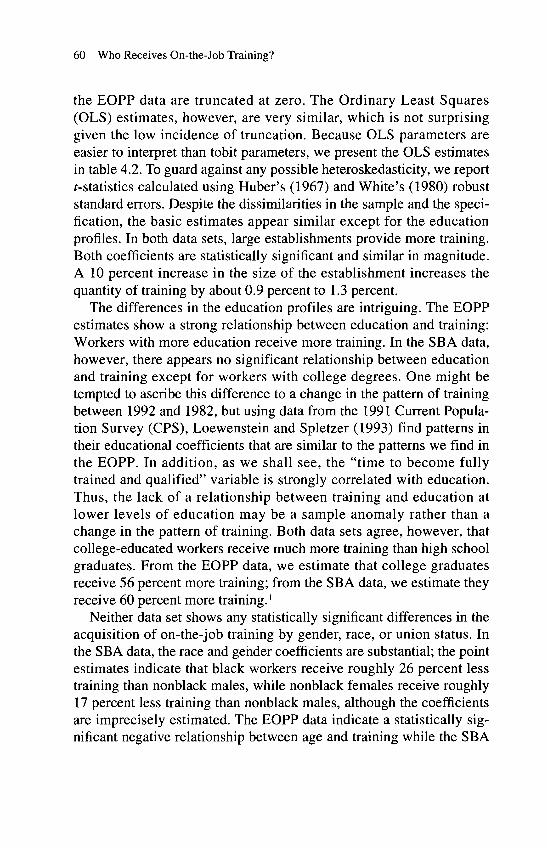
60 Who Receives On-the-Job Training?
the EOPP data are truncated at zero. The Ordinary Least Squares (OLS) estimates, however, are very similar, which is not surprising given the low incidence of truncation. Because OLS parameters are easier to interpret than tobit parameters, we present the OLS estimates in table 4.2. To guard against any possible heteroskedasticity, we report ^-statistics calculated using Huber©s (1967) and White©s (1980) robust standard errors. Despite the dissimilarities in the sample and the speci fication, the basic estimates appear similar except for the education profiles. In both data sets, large establishments provide more training. Both coefficients are statistically significant and similar in magnitude. A 10 percent increase in the size of the establishment increases the quantity of training by about 0.9 percent to 1.3 percent.
The differences in the education profiles are intriguing. The EOPP estimates show a strong relationship between education and training: Workers with more education receive more training. In the SBA data, however, there appears no significant relationship between education and training except for workers with college degrees. One might be tempted to ascribe this difference to a change in the pattern of training between 1992 and 1982, but using data from the 1991 Current Popula tion Survey (CPS), Loewenstein and Spletzer (1993) find patterns in their educational coefficients that are similar to the patterns we find in the EOPP. In addition, as we shall see, the "time to become fully trained and qualified" variable is strongly correlated with education. Thus, the lack of a relationship between training and education at lower levels of education may be a sample anomaly rather than a change in the pattern of training. Both data sets agree, however, that college-educated workers receive much more training than high school graduates. From the EOPP data, we estimate that college graduates receive 56 percent more training; from the SBA data, we estimate they receive 60 percent more training. 1
Neither data set shows any statistically significant differences in the acquisition of on-the-job training by gender, race, or union status. In the SBA data, the race and gender coefficients are substantial; the point estimates indicate that black workers receive roughly 26 percent less training than nonblack males, while nonblack females receive roughly 17 percent less training than nonblack males, although the coefficients are imprecisely estimated. The EOPP data indicate a statistically sig nificant negative relationship between age and training while the SBA

On-the-Job Training 61
does not, although the coefficient in the SBA data is insignificantly negative. Also, the SBA data indicate that firms with more off-site employees provide more training to these employees, although the magnitude of the coefficient is about one-third the size of the coeffi cient for the size of the establishment.
In columns (2) and (4), we include hours of work as a control to explore the relationship between hours worked and training. In both data sets, employees who work longer hours receive more training, and both coefficients are statistically significant and similar in magnitudes. A 10 percent increase in the number of hours worked increases the amount of training about 7.5 percent to 8.1 percent. These estimates, however, should be viewed with a healthy dose of skepticism. Hours of work are clearly the result of a decision made between the firm and the worker. If a position requires a more highly trained worker, both firm and worker have an incentive to increase the hours of work for that position.
We use a similar specification to examine the determination of the number of months to become fully trained and qualified, or what we refer to as "the total human capital" of the job. OLS estimates for the total human capital measures from the SBA and EOPP data are pre sented in columns (1) and (3) of Table 4.3. We again use a double log specification, and we add one to each observation to avoid taking the logarithm of zero. In the SBA data, 12 observations are censored at zero, and in the EOPP data, 38 observations are truncated at zero. We initially used a tobit procedure to estimate the parameters, but because the OLS estimates were quite similar and easier to interpret, we report them. We again calculate the /-statistics using the robust standard errors suggested by Huber (1967) and White (1980).
Interestingly, the coefficients on experience are both positive and significant in both data sets, and their magnitudes are similar. Unlike the training equations, the coefficients on the education dummies exhibit the same pattern in the two data sets: the total human capital of the job appears to be increasing in the worker©s education. While the coefficient for some college experience from the SBA data is about a sixth the size of the corresponding coefficient from the EOPP data, the coefficients on high school dropouts and college graduates are of simi lar magnitudes in both data sets. The coefficient on establishment size

62 Who Receives On-the-Job Training?
is negative and significant for the EOPP data, but is positive and not significant in the SBA data.
Unlike the training equations, the gender and race dummies indicate a difference in the job©s total human capital by race and gender. For the EOPP data, women occupy jobs that require about 36 percent less time to become fully trained and qualified. In the SBA data, the race con trols make for even more dramatic differences. Blacks occupy jobs that take about 58 percent less time, and nonblack women occupy jobs that take about 46 percent less time to become fully trained and qualified than nonblack males. 2 Thus, although there is no statistically signifi cant evidence that minority workers receive less training than nonblack males or that women receive less training than men in the first three months of employment, there is considerable evidence that black workers and nonblack women occupy jobs with a good deal less total human capital than nonblack men.
Columns (2) and (4) of table 4.3 include hours of work as a control in the model specification. The inclusion of the hours variable reduces somewhat the coefficients for blacks, nonblack women, and women, but the coefficients remain highly significant. Thus, the fact that women work fewer hours than men explains only a small portion of the gender difference in the total human capital of jobs.
The use of these two different training measures, total hours of training in the first three months and the time to become fully trained and qualified, gives two pictures of the workers© access to on-the-job training. There may be differences in the type of training that we mask in our use of hours of training. For instance, if we think of training dif fering in quality, we might expect that blacks and nonblack women are systematically sorted into jobs that provide low-quality training, while nonblack males have access to jobs with high-quality training. An obvious limitation of the hours of on-the-job training measure is that it includes only the training received in the first three months of employ ment. As we saw in chapter 3, data from the NLSHS72 and NLSY sug gest that the distributions of training spells have extremely long tails. Moreover, by focusing on the training received in the first three months, data sets, such as the SBA and EOPP surveys cut off that long tail, which may cause us to miss racial and gender differences in train ing when using the hours of training measures. 3

63
Table 4.3 Time to Become Fully Trained and Qualified for the 1992 SBA and 1982 EOPP Data
Independent variables
Constant
Logarithm of worker©s age
Logarithm of worker©s relevant experience
Worker is a high school dropout
Worker has some college
Worker is a college graduate
Worker is black
Worker is nonblack female
Worker is female
Union
Logarithm of number of employees at the establishment
Logarithm of number of employ ees at otherestablishments
Logarithm of hours worked
R2
N
SBA(1)
1.176*(2.41)0.289*
(1.99)
0.222* (4.10)
-0.432* (3.34)0.038
(0.39)0.525*
(4.80)-0.804*(6.18)-0.570*(6.69)
-
-0.139(0.84)
0.029(1.22)
0.008(0.68)
~
0.162
888
SBA(2)
-2.708(4.97)0.239
(1.73)
0.174* (3.45)
-0.248* (2.06)0.120
(1.29)0.494*
(4.87)-0.712*(5.87)-0.409*(4.99)
-0.159(0.97)
-0.012(0.51)
0.012(1.06)1.160*
(11.65)0.271
888
EOPP(3)
3.032(7.26)-0.207 (1.59)
0.197* (4.17)
-0.446* (4.01)0.189*
(2.35)0.476*
(4.16)
-0.422*(6.66)0.169
(1.19)
-0.049*(2.26)
0.075
1,471
EOPP(4)
1.757(3.24)-0.206* (1.67)
0.133* (2.91)
-0.194 (1-79)0.225*
(2.91)0.463*
(4.24)
-0.253*(4.09)0.179
(1-28)
-0.066*(3.12)
-
1.323* (13.08)
0.141
1,471NOTE: Absolute values ot ^-statistics, calculated using robust standard errors, are in parentheses. Coefficients marked with an * are significant at the 5 percent level. Ordinary least squares esti mates are reported.

64 Who Receives On-the-Job Training?
With the SBA data, however, we can control for this truncation at three months because we know not only the total hours of training but also the number of weeks of training. If we were to assume that the random error term in the training equation was drawn from a particular distribution, we could estimate the training equation accounting for the truncation. For instance, if we assume that the error term was normally distributed, we could use a censored regression model. Unfortunately, the prevailing wisdom is that such estimates are somewhat susceptible to misspecification (see Greene, 1993).
Rather than risk misspecification of the distribution of the error term, we estimate a Cox model, which is based on the Lehmann alter native of nonparametric statistics. The essential idea of nonparametric statistics is to allow researchers to make inferences without having to make assumptions about the distribution of random variables. For instance, letting T denote our training measure, the regressions reported in table 4.2 and 4.3 assume a model of the form
(4.1) r = *P + e
where e is normally distributed with mean zero and variance o2, X is a vector of covariates, and ft is a vector of parameters that we wish to estimate. If the assumption about the distribution of e is true, the ordi nary least squares is the most efficient estimator of the parameters fi available. The nonparametric statistician asks the question, "How do you know that e is normally distributed?" A truthful answer is often that such an assumption is convenient.
Of course, ordinary least squares estimation may still be justified as a method of moments estimator, with the caveat that tests of hypothe ses are still going to require some additional assumptions about the second moment of the distribution. Cox (1972) recognized, however, that by focusing only on the rank of the dependent variable, parameters could be estimated and hypotheses tested without having to specify a distribution of the stochastic variable. Moreover, the Cox model easily handles the truncation of the dependent variable, a limitation that is rel evant to both the EOPP and SBA data.

On-the-Job Training 65
For the Cox model, the cumulative distribution function for the ith worker is expressed as
(4.2) F(Tpi
where F(-) is what is commonly referred to as the "baseline" cumula tive distribution function and a, is an "index" function for the ith worker. If the term a^ < 1, then the ith worker is more likely to have a short training spell, and if a^ > 1 the worker is more likely to have a long training spell. (By definition, the "baseline" cumulative distribu tion function corresponds to the distribution of training spells for the person with ai =1.) Using this approach, we must only specify the functional form of a-v or
(4.3) a-expHQp).
The Cox model, by focusing on the ranks of the dependent variable, allows the researcher to estimate ft without specifying distribution of the dependent variable.4 Thus, the Cox model affords two advantages of standard parametric estimates such as those we presented in tables 4.2 and 4.3. First, the Cox model does not require researchers to spec ify the distribution of the random variable. Second, the model allows researchers to account for the truncation of the dependent variable.
This approach is a fundamental departure from standard parametric estimation where we generally assume a probability distribution func tion of the form
(4.4)
In contrast, the Cox model has the probability density function:
(4.5) J(Th Xj) =
where f(T{) is the derivative of F(Ti). Thus, while the standard paramet ric estimators assume that the independent variables affect only the mean of the distribution of training, the Cox model assumes that the independent variables affect the entire distribution of training spells. As a result, we cannot compare the two approaches and determine

66 Who Receives On-the-Job Training?
which approach better fits the data. The Cox model, however, does pro vide an important specification check on the results that we present in tables 4.2 and 4.3. It allows us to assess the robustness of our results with respect to the truncation of the training measures at three months and to evaluate our assumptions about the distribution of the error terms.
In table 4.4, we present the results from the Cox model. The results are generally consistent with those reported in table 4.2, with a couple of notable exceptions. First, the coefficient on the logarithm of employees at other sites is not significant. Second, the coefficient on nonblack females is negative and statistically significant, indicating that nonblack women received significantly less training than nonblack males. The coefficient on black workers, while not statistically signifi cant, is about the same magnitude as the coefficient on nonblack females. Moreover, the lack of significance on the black coefficient is not a robust result. In Barren, Berger, and Black (1994), we report results using a slightly different specification and a larger sample size where the coefficient on black workers is negative and significant in a Cox model.5 Using the EOPP data, Barron, Black and Loewenstein (1993) report that while women were placed in less complex jobs, they did not receive less training than males; in tables 4.2 and 4.3, we obtained similar results. In our view, these results should be viewed with suspicion. When we do not account for the truncation of training at three months, we obtain a similar result for the SBA data; therefore, we cannot reject the hypothesis that nonblack females receive the same quantity of training as nonblack males. Accounting for the truncation of training, however, reverses this result. 6 This suggests that research ers should be extremely careful when viewing racial and gender differ ences with truncated data.
One final finding of interest concerns the considerable change in the distribution of wages in the time between the EOPP and SBA samples. Blackburn, Bloom, and Freeman (1990); Katz and Murphy (1992); Becker (1992); and Berger (1992) document an increase in the returns to higher education during the 1980s. Juhn, Murphy, and Pierce (1993) show that in the 1970s and 1980s wages become much more disperse, with low-wage workers experiencing a fall in real wages while workers from the upper end of the distribution saw a growth in real wages. Given these fundamental changes in the distribution of wages, one

On-the-Job Training 67
might anticipate that changes in the distribution of on-the-job training are responsible for some of the changes in the distribution of wages. Surprisingly, we find little evidence for this hypothesis. The EOPP and SBA data sets provide reasonably consistent answers to the question of who receives training despite the ten-year difference in the age of the surveys. Thus, researchers will have to look beyond differences in training at least training in the first three months of employment to explain the dramatic increase in earnings inequality.
Table 4.4 Total Hours of Training for the 1992 SBA Data, Cox Model
Independent variables SBA
Logarithm of worker©s age
Logarithm of worker©s relevant experience
Worker is a high school dropout
Worker has some college
Worker is a college graduate
Worker is black
Worker is a nonblack female
Union
Logarithm of number of employees at establishment
Logarithm of number of employees at other establishments
Chi-squared statistics
N_______________ __NOTE:. Absolute values of z-statistics are in parentheses. Coefficients marked with an * are sig nificant at the 5 percent level.
-0.021 (0.13)
-0.050 (0.93)-0.118 (0.75)
-0.106 (1.09)0.478*
(4.24)
-0.222 (1.50)-0.203* (2.33)
0.108 (0.69)0.060*
(2.40)
0.011 (0.87)
59.75

68 Who Receives On-the-Job Training?
In the next section, we explore the determination of the incidence of training. This exercise will allow us to compare our results to many studies where the measures of training are binary (e.g., 1983 CPS data). In addition, it will allow us to examine differences in the inci dence of each type of training.
Variations in the Incidence of Training
The incidence of training is inherently a dichotomous variable. Workers either receive a certain type of training or they do not. Because the incidence of training is a binary variable, we employ a logit proce dure. In table 4.5, we present the logit estimates for the probability of receiving off-site formal training. The coefficient from a logit model may be interpreted as the rate of change in the logarithm of the ratio of probability that the variable is one, which we denote P, divided by the probability the variable is equal to zero, which we denote (1 - P). The logarithm of the ratio of these two probabilities is often referred to as the "log odds© ratio." To convert this coefficient to a derivative of the probability, it is necessary to multiply the coefficient by P(l - P). About the sample mean, this can be easily done by referring to the mean incidence rates in table 4.1. For instance, evaluated about the mean, a worker with a college degree increases the probability of off-site train ing by about 0.122 [1.272 x 0.107(1 - 0.107)], or a worker with a col lege degree more than doubles the probability of receiving off-site training. The relationship among training, the size of the establishment, and the number of workers at other sites provides some insights into training decisions. Larger establishments tend to be less likely to pro vide off-site training to their employees, although the coefficient is not quite significant at the 10-percent level. In contrast, the larger the num ber of employees at other sites, the more likely the firm will offer off- site formal training, perhaps sending their newly hired workers to other company sites.
Table 4.6 presents logit estimates for the probability of receiving on- site formal training for the SBA and EOPP data. The two sets of esti mates have some interesting similarities and dissimilarities. Both data sets indicate that college graduates are more likely to receive on-site

69
Table 4.5 Incidence of Off-Site Formal Training for the 1992 SBA Data
Independent variables
Constant
Logarithm of worker©s age
Logarithm of worker©s relevant experience
Worker is a high school dropout
Worker has some college
Worker is a college graduate
Worker is black
Worker is a nonblack female
Union
Logarithm of number of employees at establishment
Logarithm of number of employees at other establishments
Chi-squared statistics
N
SBA
-2.055(1.27)
-0.200(0.40)
-0.067(0.44)
-0.424(0.66)
0.426(1.37)
1.272*(4.46)
-0.529(1.02)
0.064(0.28)
0.760*(2.23)
-0.106(1.56)
0.108*(3.16)
43.21
888NOTE: Absolute values of z-statistics are in parentheses. Coefficients marked with an * are signif icant at the 5 percent level. Logit estimates are reported.

70
Table 4.6 Incidence of On-Site Formal Training for the 1992 SBA and 1982 EOPP Data
Independent variables
Constant
Logarithm of worker©s age
Logarithm of worker©s relevant experience
Worker is a high school dropout
Worker has some college
Worker is a college graduate
Worker is black
Worker is a nonblack female
Worker is female
Union
Logarithm of number of employees at establishment
Logarithm of number of employees at other establishments
Chi-squared statistics
NNOTE: Absolute values of z-statistics are in parentheses, icant at the 5 percent level. Logit estimates are reported.
SBA
-2.059*(1.97)
-0.017 (0.05)
-0.195 (1.85)
0.523 (1.72)
0.062 (0.31)0.639*
(3.21)
0.181(0.63)
0.250(1.52)
0.686*(2.64)0.170*
(3.64)0.107*
(4.56)
94.52
888Coefficients marked with an
EOPP
-1.997(1.88)
-0.163 (0.49)
-0.012 (0.11)
-0.321 (1.03)0.541*
(2.87)0.617*
(2.56)
-0.070(0.44)
-0.190(0.61)0.160*
(3.04)
25.58
1,471* are signif-

On-the-Job Training 71
formal training than are high school graduates the differential is about 0.13 for the SBA and about 0.07 for the EOPP. Similarly, larger establishments are more likely to offer formal training; a doubling of the establishment size increases the probability of training by 0.036 for the SBA data and by 0.018 for the EOPP data.
The EOPP data indicate, however, that those workers who attended but did not complete college have about the same probability of under going formal training as college graduates; indeed, we cannot reject the hypothesis that the two groups have the same incidence of training. In contrast, the SBA data indicate that college graduates do have a higher incidence of training than high school graduates. Similarly, for the SBA data, we cannot reject the hypothesis that high school dropouts have the same incidence of on-site formal training as college gradu ates, but for the EOPP data, that hypothesis is easily rejected.
For the SBA data, we find that union members are more likely to receive on-site formal training than nonunion members; the differential is about 0.14. In contrast, in the EOPP data, firms with unions appear to be no more likely to offer on-site formal training than firms without unions. Thus, for the SBA data, union members appear to receive more off-site and on-site formal training. This result contrasts with the find ings of Mincer (1983), who uses the 1978 PSID data; Barren, Feuss, and Loewenstein (1987), who use the 1982 EOPP data; and Lillard and Tan (1992), who use the 1983 CPS data. All of these studies find that union members receive less training than nonunion workers. Lynch (1992) and Veum (1993), using data from two different time periods of the NLSY, report that union members are more likely to receive formal training. Loewenstein and Spletzer (1993), using 1991 CPS data, report that, in a parsimonious specification that includes only race, gender, marital status, and education controls, union members are more likely to receive training than nonunion members, but the coeffi cient on union membership becomes insignificant yet still positive once controls for experience and tenure are included.
There are at least two potential explanations for the differences in these findings. First, differences in the sampling strategies might pro vide one rationale. Both the SBA and the NLSY have younger samples than the CPS or the PSID, although the EOPP is somewhat younger than the SBA sample. This suggests that younger union members are more likely to receive formal training than young nonunion members,

72 Who Receives On-the-Job Training?
but this difference dissipates over time and eventually reverses itself. Given that union workers have lower turnover probabilities than non union members, there is less reason to delay training among union members than among nonunion members.
Changes in the union sector in the last decade may provide another explanation. With the importance of international trade in the United States economy, there has been a rapid reduction in the domestic man ufacturing sector of the economy, as other countries have assumed many semiskilled manufacturing jobs previously performed in the United States. A corresponding decrease in union membership has accompanied this trend. Given the United States© relatively advanced educational system and given that on-the-job training and education appear to be positively correlated, it may be that the United States© comparative advantage lies in jobs that require workers to obtain sig nificant amounts of on-the-job training. If competitive pressures have eliminated the low-training union jobs, the difference between the 1982 EOPP data and the 1992 SBA data may indicate that there has been a structural shift in the economy.
With informal management training, it is important to remember that the incidence is quite high about 92 percent for the SBA data and about 87 percent for the EOPP data. There are, therefore, few workers whom managers do not informally train. Table 4.7 presents the logit estimates for the probability of obtaining informal manager training for the SBA and EOPP data. Not surprisingly, we cannot reject the hypoth esis that all the coefficients are insignificant for the SBA data. For the EOPP data, only two coefficients are significant. Workers with more experience are less likely to receive training, and larger establishments are more likely to offer this type of training.
For informal co-worker training, both the SBA and the EOPP data indicate that larger establishments are more likely to offer co-worker training. Table 4.8 presents the logit estimates for the two data sets. Evaluated at the sample means, a 100 percent increase in the size of the establishment increases the probability of co-worker training by 0.056 for the SBA data and 0.058 for the EOPP data. This finding probably reflects the fact that larger establishments are more likely to have a worker performing similar tasks, which reduces the cost of co-worker training. There are some minor differences in the two data sets. The EOPP results suggest older workers are less likely to receive co-worker

73
Table 4.7 Incidence of Informal Management Training for the 1992 SBA and 1982 EOPP Data
Independent variables
Constant
Logarithm of worker©s age
Logarithm of worker©s relevant experience
Worker is a high school dropout
Worker has some college
Worker is a college graduate
Worker is black
Worker is a nonblack female
Worker is female
Union
Logarithm of number of employees at establishment
Logarithm of number of employees at other establishments
Chi-squared statistics
NNOTE: Absolute values of z-statistics are in parentheses, icant at the 5 percent level. Logit estimates are reported.
SBA
2.454(1.50)
0.058 (0.11)
-0.179 (1.09)
-0.577 (1.24)
-0.536(1.77)
0.060 (0.17)
-0.087(0.18)
-0.095(0.36)
0.224(0.41)
0.064 (0.80)
0.008 (0.21)
9.21
888
EOPP
2.525*(2.55)
-0.291 (0.94)-0.262*
(2.54)
-0.101 (0.39)
0.191 (0.91)
-0.037 (0.14)
-0.043(0.27)
-0.099(0.30)0.218*
(3.72)
30.93
1,471Coefficients marked with an * are signif-

74
Table 4.8 Incidence of Informal Co-Worker Training for the 1992 SBA and 1982 EOPP Data
Independent variables
Constant
Logarithm of worker©s age
Logarithm of worker©s relevant experience
Worker is a high school dropout
Worker has some college
Worker is a college graduate
Worker is black
Worker is a nonblack female
Worker is female
Union
Logarithm of number of employees at establishment
Logarithm of number of employees at other establishments
Chi-squared statistics
NNOTE: Absolute values of z-statistics are in parentheses, icant at the 5 percent level. Logit estimates are reported.
SBA(1)
0.857 (0.87)
-0.323 (1.07)
-0.165 (1.70)
0.317 (1.02)
0.211 (1.13)
0.312 (1.54)0.021
(0.07)
0.151 (0.94)
-0.253 (0.90)0.265*
(5.21)
0.044 (1.79)
63.55
888
EOPP(2)2.313*
(3.31-0.769* (3.50)
0.055 (0-74)
0.006 (0.03)
0.080 (0.56)
-0.244 (1.31)
0.117 (1-04)
0.074 (0.32)0.247*
(6.17)
72.77
1,471Coefficients marked with an * are signif-

On-the-Job Training 75
training, and the coefficient for the worker©s age is highly significant. In the SBA, while the coefficient for the worker©s age is negative, it is not significant. The coefficients for college-educated workers have the opposite signs in the two data sets, although neither is significantly dif ferent from zero.
Finally, both data sets again indicate a preference for "watching oth ers" training among larger establishments. The logit estimates for the SBA and EOPP data are given in table 4.9. Evaluated at the sample means, a 100 percent increase in the size of the establishment increases the likelihood of this type of training by 0.029 in the SBA data and 0.027 in the EOPP data. Again, there are some minor differences in the two data sets. For the EOPP data, workers with more experience are less likely to undergo training by "watching others," while the same coefficient for the SBA data is negative but not significant. Similarly, for the EOPP data, workers with some college education are more likely to "watch others," while the same coefficient for the SBA data is positive but not significant.
Taken together, the two data sets provide a reasonably similar description of the incidence of the various types of training. Three major themes run through these regressions. First, large firms have higher rates of training incidence. These establishments tend to be more likely to offer formal on-site training, informal co-worker train ing, and training by watching others. Also, the EOPP data indicate that larger establishments are more likely to offer informal management training, and the SBA data indicate that firms with larger numbers of employees at other sites were more likely to offer off-site formal train ing. Second, both the SBA and EOPP data agree that college graduates are more likely to receive formal training than are high school gradu ates. And finally, the SBA data indicate that union members are more likely to receive formal training, but the EOPP does not provide any evidence of this differential.
Truncated Spells of Training
Because the SBA survey asked for the number of weeks of training and the number of hours of training per week, we may also assess how

76
Table 4.9 Incidence of Training by Watching Others for the 1992 SBA and 1982 EOPP Data
Independent variables
Constant
Logarithm of worker©s age
Logarithm of worker©s relevant experience
Worker is a high school dropout
Worker has some college
Worker is a college graduate
Worker is black
Worker is a nonblack female
Worker is female
Union
Logarithm of number of employees at establishment
Logarithm of number of employees at other establishments
Chi-squared statistics
N
SBA(1)
1.026(1.06)
-0.221 (0.74)
-0.115 (1.21)
0.158 (0.52)
0.191 (1.03)
-0.017 (0.08)
0.209(0.73)
0.060(0.39)
-0.047(0.17)0.133*
(2.83)
0.022 (0.92)
20.24
888NOTE: Absolute values of z-statistics are in parentheses. Coefficients marked with an icant at the 5 percent level. Logit estimates are reported.
EOPP(2)
0.978(1.12)
0.029 (0.11)-0.282*
(3.10)
-0.051 (0.23)0.396*
(2.11)
-0.271 (1.26)
0.253(1.82)
-0.352(1.36)0.180*
(3.67)-.
39.96
1,471* are signif-

On-the-Job Training 77
many spells of training are truncated by the three-month time frame. For the SBA data, we treat any spell lasting at least 12 weeks as trun cated. 7 Conditional on receiving each type of training, the rates of trun cation are 0.19 for off-site formal training, 0.16 for on-site formal training, 0.24 for informal management training, 0.26 for co-worker training, and 0.19 for "watching others." We have seen in chapter 3 that data from the NLSY and NLSHS72 indicate that many spells of formal training last beyond three months. Also, while the NLSHS72 data had an extremely low incidence rate of informal training, many spells of informal training were longer than three months. The SBA data indi cate that informal training spells are also likely to last at least 12 weeks.
In table 4.10, we present logit estimates of the probability for each type of training that a training spell lasts at least 12 weeks. In column (1), we list the estimates for the off-site formal training. Only one of the coefficients is significant at the 5 percent level. Nonblack females are less likely than nonblack males to have undergone off-site training spells that last at least 12 weeks. Evaluated at the sample means, non- black women©s probability is about 0.30 smaller than nonblack men©s. Thus, the truncation of the training measure at three months hides the gender differences in the off-site training variable. In column (2), we present the estimates for on-site formal training, and again, only one coefficient is statistically significant at the 5 percent level. Nonblack females are less likely to have on-site training spells that last at least 12 weeks than are nonblack males. Evaluated at the sample means, non- black women©s probability is about 0.12 lower than nonblack men©s. Thus, for both formal training measures, nonblack women are less likely to experience a long spell of formal training, and the truncation of the training measures at three months hides the true gender differen tial. We also note that while the coefficient on blacks in the on-site for mal training equation is not statistically significant, it is much larger than the nonblack female coefficient. Because there are only a limited number of blacks in the sample, it is difficult to obtain a precise esti mate of the coefficients, and the reader should not interpret the insig nificance of the coefficient as strong evidence that blacks are as likely as nonblack males to have long spells of on-site formal training.
Also in both formal training equations, it was necessary to eliminate the high school dropouts because no high school dropout had a spell of

Table 4.10 Incidence of Training Spells Lasting at Least 12 Weeks for the 1992 SBA Data
Independent variablesConstant
Logarithm of worker©s age
Logarithm of worker©s relevantexperience
Worker is high school dropout
Worker has some college
Worker is college graduate
Worker is black
Worker is nonblack female
Union
Off-site formal
training(1)4.560
(0.85)-1.293(0.75)
0.499(1.20)
-1.185(1.24)-0.308(0.41)1.395
(1.04)-1.928*(2.64)1.249
(1.58)
On-site formal
training(2)
0.645(0.24)-0.018(0.02)
0.311(1.30)
-0.486(0.94)0.352
(0.87)-1.126(1.38)-0.866*(2.30)0.445
(0.95)
Informal manager training
(3)-1.703(1.54)0.263
(0.77)
-0.125(1.13)-0.257(0.72)-0.520(2.25)0.605*
(2.98)-0.489(1.44)-0.242(1.39)0.189
(0.66)
Informal co-worker training
(4)-0.718(0.54)-0.054(0.37)
0.196(1.54)0.008
(0.02)0.010
(0.04)0.852*
(3.60)-0.201(0.55)-0.224(1.14)0.397
(1.24)
Train by watching
others(5)1.974
(1.37)0.234
(0.53)
-0.022(0.16)-0.073(0.16)-0.029(0.10)1.061*
(4.04)-0.350(0.82)-0.256(1.17)-0.234(0.59)

Logarithm of number of employees at establishmentLogarithm of number of employees at other establishmentsChi-squared statisticN
-0.292 (1.47)-0.111 (1.17)21.77
92
-0.164 (1.65)-0.034 (0.64)18.98244
-0.019 (0.38)-0.006 (0.24)30.58817
-0.028 (0.47)-0.026 (0.90)25.95617
-0.106 (1.63)0.002
(0.05)26.14611
NOTE: Absolute values of z-statistics are in parentheses. Coefficients marked with an * are significant at the 5 percent level. Logit estimates are reported.

80 Who Receives On-the-Job Training?
training lasting at least 12 weeks. As such, dropping out of high school perfectly predicts that the training spell is not truncated. The estimation procedure cannot determine a coefficient, and so it is necessary to drop the observations. In the case of off-site formal training, we exclude only three cases, and we should not overemphasize this exclusion. In the case of on-site formal training, however, we exclude 23 cases, which makes it highly likely that dropouts are less likely to have long spells of training. Given that dropouts have revealed an aversion to or a lack of aptitude for formal schooling, it is not surprising that they pos sess jobs that do not require long spells of formal training.
Column (3) presents the logit estimates for the probability of under going a spell of formal management training lasting at least 12 weeks. Two coefficients are significant at the 5 percent level. Workers who attended but did not graduate from college are less likely to have a long spell of informal management training than are high school graduates. At the sample mean, a high school graduate has a 0.096 higher proba bility of having a truncated spell of informal management training than a worker with some college education. This finding further demon strates that the SBA sample of workers with some college education is somewhat anomalous because almost all other studies have found that training increases with education. Workers with college degrees, on the other hand, are more likely to have a truncated spell of informal man agement training. Evaluated at the sample mean, college-educated workers have about a 0.112 higher probability of undergoing a spell of informal management training that lasts at least 12 weeks than do high school graduates.
In columns (4) and (5) of table 4.10, we present the logit estimates for the co-worker training and "watching others" equations. In both equations, only one coefficient is significant at the 5 percent level: col lege graduates have a greater chance than high school graduates of undergoing a training spell that lasts at least 12 weeks. Evaluated at the sample means, the college graduates have a 0.164 greater probability of undergoing a training spell that lasts at least 12 weeks for both train ing measures than do high school graduates. Thus, for each type of informal training, college graduates have a significantly higher proba bility of undergoing a spell lasting at least 12 weeks than do high school graduates. This suggests that the 43 percent differential in the number of hours of total training between college graduates and gradu-

On-the-Job Training 81
ates of only high school understates the true differentials in the training experiences of newly hired employees.
Thus, the three-month sampling frame of the EOPP data and the SBA data appears to have two major consequences. First, the sampling frame may hide a gender differential in formal training measures. Non- black women are significantly less likely to have formal training spells that last at least 12 weeks than are nonblack men. Second, the sampling frame also understates the training differential that college graduates receive; college graduates are significantly more likely to have infor mal training spells that last at least 12 weeks than are high school grad uates.
Conclusions
There are four conclusions that emerge from both the EOPP and SBA data. First, college graduates receive much more training than high school graduates. Even after controlling for other factors, college graduates receive between 56 to 60 percent more training than high school graduates in the first three months of employment. Moreover, analysis of the SBA data suggests that this difference is understated because college graduates are more likely to have their training spells continue past three months. When labor economists estimate the returns to college education without controls for on-the-job training, perhaps some of the presumed return to college education may be a return to the greater quantities of on-the-job training.
Second, when hiring workers for more complex jobs, firms appar ently hire workers with greater prior relevant work experience for a couple of reasons. First, firms may find it more expensive to train workers themselves than to hire experienced workers. This would be especially true for positions in which the worker was expected to "learn by doing," or learn by actually performing the task at hand. Sec ond, by hiring experienced workers, firms may reduce the risk that they have hired a worker who is incapable of doing the job. As we shall see in chapter 7, firms spend much more time evaluating workers when hir ing for jobs with more training and greater total human capital.

82 Who Receives On-the-Job Training?
Third, we find evidence that large establishments offer more train ing, which might explain some of the wage premium earned by work ers at these larger sites. We find that a 10 percent increase in the size of the establishment increases the hours of training in the first three months of employment by about 0.9 percent to 1.3 percent. Larger establishments are also more likely to offer on-site formal training than are smaller establishments, and using the SBA data, we find some evi dence that employees of large firms who work at small sites are more likely to undergo off-site training, as they presumably receive training at larger sites within the firm.
Finally, both data sets indicate substantial gender difference in the time to become fully trained and qualified, and the SBA data indicate a substantial racial difference in the time to become fully trained. Even after we control for other factors, blacks hold jobs that require about 60 percent less time to become trained and qualified while nonblack women occupy jobs that require between 36 and 46 percent less time than the jobs of nonblack males. Interestingly, we find that the trunca tion in the hours of training may hide gender differences in hours of training; women are significantly less likely than men to have spells of formal training that last longer than three months.
NOTES
1. We use the adjustment that Kennedy (1991) develops, where the differential g is approxi mated by g = exp[$ - 0.5 VAR $ ) ] - 1.
2. Again, we sue the adjustment that Kennedy (1991) develops to estimate the differential.3. The time to become fully trained, however, also suffers from some biases. The time variable
does not measure the intensity of training, and the intensity of training may vary by the type of job. Moreover, certain jobs may require very little training, but workers may take a great deal of time to master fully the tasks that the job requires; they may learn by actually doing the job. Other jobs may require workers to be continuously in training while becoming fully trained and quali fied, thus, two workers may take the same time to be fully qualified but may have much different training experiences. Because of these limitations, we interpret the "time to become fully trained" variable as a measure of a job©s total human capital rather than as a measure of on-the-job train ing. As wel shall see in chapter 6, the evidence from wage growth equations supports this view: wage growth is more highly correlated with total hours of training than the time to become fully trained and qualified.
4. See Kalbfleisch and Prentice (1980) for details of the estimation procedure.5. Given the similarity in magnitude, the reader may wonder if the two groups should be
pooled. We cannot reject the hypothesis that the coefficients on black and nonblack female work ers are the same. If we do pool these two groups, the coefficient is negative and significant with a z-statistic of-2.43.

On-the-Job Training 83
6. As in the OLS case, controlling for hours reduces the magnitude of the coefficient on non- black female workers and eliminates its statistical significance. When controlling for hours, the coefficient is -0.121 with az-statistic of-1.38.
7. Although there are 13 weeks in a three-month period, there was an unusually large fre quency of responses at 12 weeks, indicating that many respondents used a 12-week horizon.


CHAPTER J_____________
How Well Do We Measure On-the-Job Training?The Upjohn Institute Survey
In previous chapters, we examined different employer and employee measures of training and studied who receives training. This chapter addresses the issue of how well training is measured. In particular, we examine the causes and consequences of errors in the measurement of training. Several studies in the last few years have considered this issue, but most have examined the impact of measurement error on the estimation of wage equations; none has analyzed measurement errors in training, or the effects of training measurement errors on the esti mated returns to training in wage equations. Consequently, economists are lacking information on how accurately training can be measured and on the consequences of the mismeasurement of training.
To examine measurement error issues, we designed and imple mented a new survey that matches employer and employee responses to training questions. This survey permitted analysis not only of errors in the measurement of training, but also wages, productivity, and other commonly used variables in labor economics. This new data set allows us to address several questions: How accurate are measures of on-the- job training? Do employers© and employees© responses to identical questions concerning on-the-job-training differ? If answers to these common questions do differ, who reports more training? Do firm and worker responses to formal training questions show more agreement than responses to informal training questions?
The Upjohn Institute commissioned this new survey, which we con ducted in spring 1993. Approximately 300 firms and workers partici pated in the survey. Each firm was asked about its last worker hired,
85

86 How Well Do We Measure On-the-Job Training?
and we conducted interviews with both the firm and the worker. Mea surement error is more apparent for some variables than others. Figure 5.1 shows the scatterplot of firm and worker starting wages.
Workers and firms agree for the most part on the rate of pay at the start of employment. In fact, the correlation between worker and firm reports is 0.974. The level of agreement between the worker and the firm is somewhat lower for hours worked per week and months of rele vant experience prior to employment. The scatterplots for these vari ables are shown in figures 5.2 and 5.3. The correlation between worker and firm reports for hours worked is 0.769 and 0.727 for months of rel evant experience. Firms and workers disagree to an even greater extent about the amount of training provided. Figure 5.4 shows the scatterplot of worker and firm reports of total hours of training provided in the first four weeks of employment. The correlation coefficient is 0.475. Firms report 25 percent more hours of training on average than do workers, although firms and workers report similar incidence rates.
In the remainder of this chapter, we first examine previous measure ment error studies in labor economics and then describe our new data set. The results of the survey are then discussed, beginning with the correlations between employer and employee responses for a number of variables considered in previous studies. We then turn to an analysis of the measurement of on-the-job training. Finally, we examine the determinants of training and the correlates of differences in employer- and employee-reported training.
Previous Validation Studies in Labor Economics
A number of papers have considered the issue of reporting errors. Mellow and Sider (1983) use an employer-employee matched supple ment taken from the 1977 January Current Population Survey (CPS) and the first wave (1980) of the Employment Opportunity Pilot Project (EOPP). While there is a fair amount of disagreement between employers and employees on industry and occupation, it appears to have little effect on cross-section wage structure. Further, the structure of wages is independent of whether employer- or employee-reported wages are used.

Figure 5.1 Firm- and Worker-Reported Wages
87
37.0192 ~
3.25Worker-reported wage
30.4487
Figure 5.2 Firm- and Worker-Reported Hours Worked
55 -
a -
O OQ0 O O
o° co
°oo8 8°ooo
-o oo oo ono°8
o o o oo o oo
o o
Worker-reported hours75

Figure 5.3 Firm- and Worker-Reported Experience
20 -
0 -
o o o o oO 00
o o o o o
o o o8 0 o o o
Q Qo o o o oD Ooo o o o o o o o o o
Worker-reported experience35
Figure 5.4 Firm- and Worker-Reported Training
440 -
0 -
Worker-reported training448

On-the-Job Training 89
Greenberg and Halsey (1983) investigate the effects of reporting error in the Seattle and Denver income maintenance experiments by comparing employer reports with respondent self-reports. Previous studies based on respondent self-reports find appreciable reductions in work efforts by those eligible for experimental income maintenance payments. Using employer-reported data, they find that the reductions in the work effort of husbands, wives, and young workers who are not heads of households are much smaller than the self-reported data would imply. The estimates for female heads appear to be unaffected by reporting error.
Freeman (1984) examines differences in reporting union status between worker and firm reports. He uses the 1977 January CPS employer-employee matched data as well as the 1979 May CPS regular survey and the pension supplement. Assuming differences between employer and worker reports are the result of measurement error, he argues that such error may negate the value of using longitudinal data to estimate union wage effects because the measurement error biases the union wage effects downward.
Duncan and Hill (1985) use a unique set of data from a single manu facturing company that provides unprecedented detail on the work his tory of employees. They compare administrative records with information obtained from a sample of workers as a validation exercise for the Panel Study of Income Dynamics (PSID). They report estimates of wage equations that include schooling and tenure using both worker and firm reports. They find a bias of 30 percent in the estimated return to tenure due to the correlation between measurement error and tenure.
In related work, Lillard, Smith, and Welch (1986) examine measure ment error induced by the Census Bureau imputation procedure used to fill in missing observations in the CPS. They find that the Census imputation procedure severely understates income in some occupa tions. Because the evidence suggests that nonreporting is tied to income, the imputation procedure also probably causes an understate ment of average income.
Bound and Krueger (1991) use matched CPS-Social Security data to examine the prevalence of measurement error. They find that measure ment error in panel data is not as significant as previously thought because positive serial correlation and mean reversion of the measure ment error increase the reliability of panel earnings data.

90 How Well Do We Measure On-the-Job Training?
Bound, Brown, Duncan, and Rodgers (1990, 1994) also use the matched CPS-Social Security data and a later wave of the PSID valida tion survey. They find annual earnings to be fairly reliably estimated. Hourly earnings estimates are quite unreliable, however, because hours worked are imprecisely reported. Rodgers, Brown, and Duncan (1993) also examine errors in survey reports of earnings, hours worked, and hourly wages using the two waves of the PSID validation study. They find that measures of hourly earnings are "distressingly unreliable," arguing their findings suggest the importance of measurement error.
A New Validation Survey
None of the studies described in the previous section considers errors in reporting on-the-job training, or the effects of reporting errors on the estimated returns to training. Our survey, conducted in the spring of 1993, obtained evidence on this question from employers and employees. A major focus of the survey (hereafter referred to as the Upjohn Institute survey) was to provide worker-firm comparisons of on-the-job training measures. Because the intensity of on-the-job train ing is likely to be highest for newly hired workers, we decided to target those workers, similar to the EOPP and SBA surveys. We asked both firms and their last worker hired a series of training questions based on those used earlier in the EOPP and SBA surveys.
One of our major concerns centered on the accuracy of responses given by employers and employees. We did not want employers or employees to have to recall details of training that took place months or even years prior to the interview. To minimize this problem, we twice interviewed employers and employees about training, once after two weeks of employment, and a second time after four weeks of employ ment. This meant that we had to conduct interviews within narrow win dows of time, within a couple days of the end of the second and fourth week of employment.
Because of the survey design, we needed to contact firms that were hiring at the time we conducted the survey. Given our experience with the EOPP and SBA surveys, we were concerned that a number of establishments, especially small ones, would be ineligible for the sur-

On-the-Job Training 91
vey simply because they were not hiring. Therefore, we eliminated establishments with fewer than 100 workers from our sample universe to increase the chances of locating suitable establishments.
We obtained a nationwide random sample of 5,000 establishments with 100 or more employees from Survey Sampling, Inc. The survey was conducted in 1993 by the Survey Research Center (SRC) at the University of Kentucky. Each of the 5,000 establishments was first sent a letter describing the survey and the general nature of the training questions. Telephone interviewing began on March 22, 1993 and was completed on June 21, 1993. In the initial interview we asked back ground information about the firm and the characteristics of the last worker hired. If firms had not hired in the past ten days or were not planning to hire soon, they were deemed ineligible for the survey and dropped from the sample. 1
Once we had completed the initial firm interview, we asked to speak with the worker. We then asked the worker a set of background ques tions similar to what we had asked the firm. The second interview of the employer and employee occurred after the employee had been with the employer for two weeks. At that time, we asked both the worker and the firm a set of questions about the training activities of the worker during the first two weeks of employment. The last interview occurred after the worker had been with the employer for four weeks. This interview consisted of the same set of questions about training as the second interview and concluded with a few questions about worker productivity and promotion probabilities.
There were a couple of drawbacks to our survey design and sam pling strategy. Restricting the original sample to establishments with 100 or more workers meant that the sample would not be nationally representative of all establishments. Second, with three interviews for both the firm and the worker, there was the potential of attrition bias. While there was some attrition, it did not appear to be a significant problem. Eighty-five percent of the worker-firm pairs that completed the initial interview completed the entire set of interviews.
Given the level of commitment required from the firm and the worker, we anticipated a much lower level of response than a typical one-time interview would provide. From our initial sample of 5,000, we did not attempt to contact 1,603 establishments due to budget con siderations. The hiring restriction eliminated a number of firms imme-

92 How Well Do We Measure On-the-Job Training?
diately from the analysis. Out of the 3,397 establishments that we attempted to contact, 1,359 reported that they were not hiring. Others were ineligible to complete the survey due to a number of reasons: 229 had disconnected phones; in 111 establishments we only received answering machines, busy signals, computer tones, or no answer in repeated attempts; 60 establishments had gone out of business; we had language communications problems with eight establishments; 76 establishments had moved or closed, and we could not obtain a new address or verify closure. These exclusions left 1,554 establishments eligible to complete the survey. Of these, 541 directly refused to partic ipate, 241 said it was against company policy to answer a survey, 255 were unwilling to let an employee participate in a survey, and 212 repeatedly scheduled callbacks, which we took as an implicit refusal. There were 258 completions of all six interviews, and 47 partial com pletions. We only counted as a partial completion those cases in which we completed at least one employer and one employee interview. The response rate of partial and full completions was approximately 20 per cent.
To compare our sample of completions with our original sample, we obtained from Survey Sampling a few characteristics of each of the establishments in our initial sample of 5,000. These included Standard Industrial Code (SIC), Metropolitan Statistical Area (MSA) code, and status, state, and establishment size code. We distinguished among four establishment size categories: 100-249 employees, 250-499 employ ees, 500-999 employees, and 1000 or more employees. To summarize the representativeness of our sample, we estimated a probit model indi cating a partial or full completion for a particular establishment. The explanatory variables consisted of eight one-digit SIC industry dum mies (The first two SIC codes were combined to avoid empty cell prob lems), eight Census region dummies, three establishment size dummies, and a MSA status dummy. This analysis indicated that there were no significant differences at the 5 percent level in the industry and establishment size composition of the completions and the original sample. The sample of completions, however, was significantly more likely to come from rural areas and from the Mountain and Pacific Census regions than the overall sample of 5,000.

On-the-Job Training 93
Correlations Between Employer and Employee Reports and Comparisons with the Results of Previous Studies
The survey provides us with two potentially inaccurate measures on the same variable. Thus, for a continuous variable of interest x, such as on-the-job training, we have the firm©s report
(5.1) y{= X{ + i/i
where yf is the firm©s report for the ith worker, X; is the true value of the variable for the ith worker, and \4 is a random error term. The survey also provides the worker©s report
(5.2) ri^Xi + u*
where yw{ is the ith worker©s report and «" is a random error term. We assume that the two random error terms are uncorrelated with each other and *,. We allow the distributions of the error terms to contain mass points at zero, which would allow for the worker and firm mea sures to agree with positive probability. We do not require that error terms have zero mean, and so the measures may be biased. In such a model, the correlation coefficient between the worker and firm reports gives a type of signal-to-noise ratio; as the variance of the worker©s or firm©s report increases, the correlation coefficient declines. In the limit ing case of degenerate distributions for both the worker©s and firm©s error terms, the correlation coefficient would be one.
We may subtract equation (5.2) from equation (5.1) to obtain
(5.3) Ayz = y{ -ywt = i/i~ uwt = AM,-.
We may use a paired Mest to test the hypothesis that E(Au) = 0. Condi tional on Ayi ^ 0, the Wilcoxon rank test examines the hypothesis that the error terms from the firm©s and worker©s measures are drawn from the same distribution, and similarly, the sign test examines if the median of the distribution of differences is zero.
To summarize differences in employer and employee reports and to facilitate comparisons of the Upjohn Institute data to other matched

94 How Well Do We Measure On-the-Job Training?
data sets, we present in table 5.1 a series of means, correlations, and significance tests of differences between employer and employee reports on a number of demographic, human capital, wage, fringe ben efit, and productivity variables. For binary variables, in addition to the employer and employee means and the correlation, we show the per centage agreements and disagreements and the results of a test of equality of means. For continuous variables, we show means, correla tions, and the results of three tests of differences in the employer and employee reports.
There is little disagreement between firm and worker race reports. Only 2.73 percent of workers and firms disagree about whether or not a worker is nonwhite and the correlation between the responses is over 0.9. We next consider employer and employee responses on whether the worker is covered by a collective bargaining agreement. The sim ple correlation between the employer and employee responses is 0.689, and the means are similar: employers report 10.5 percent of workers are covered and employees report 9.7 percent. Because the distribu tions are binomial, we use Fisher©s exact test to determine if the reported rate of unionization is the same; the one-tail p-value from Fisher©s test is 0.594, so we cannot reject the hypothesis that the rates are the same. From the 1977 January CPS employee-employer match, Mellow and Sider (1983) report that 7.1 percent of the employees dis agree with their employers on their union status. Using a somewhat smaller sample from the same data set, Freeman (1984) finds only 3.45 percent of the employees disagree with their employers on union sta tus. In the Upjohn Institute survey, 5.65 percent of the employees dis agree with their employer on collective bargaining coverage. Thus, the Upjohn Institute data appears to compare favorably with the matched 1977 January CPS data about union coverage.
Variables 3 through 10 in table 5.1 show employer and employee responses to a series of schooling completion questions. There is a fair amount of disagreement between employers and employees, and it is especially dramatic in some of the schooling categories. College atten dance, in particular, shows a massive amount of disagreement. Almost 42 percent of the observations disagree on whether the worker attended college! The correlation between the employer and employee©s reports is only 0.186. Firms are almost twice as likely to report that the worker has attended, when the worker says he or she did not attend, as are the
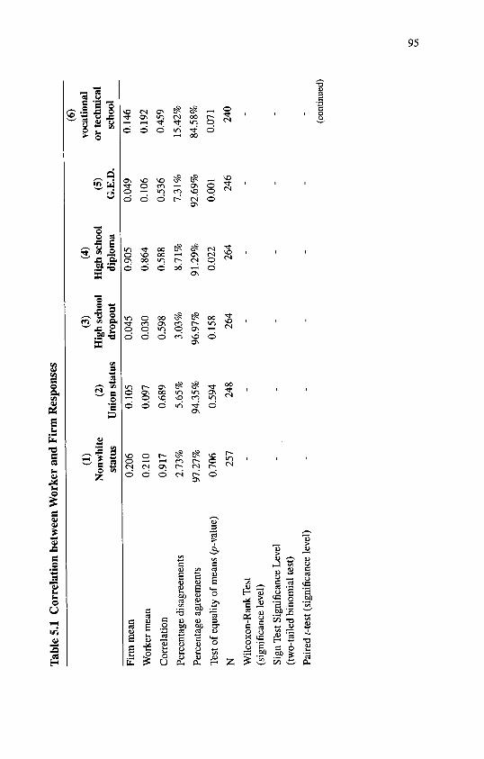
Tab
le 5
.1 C
orre
latio
n be
twee
n W
orke
r an
d Fi
rm R
espo
nses
Firm
mea
n
Wor
ker m
ean
Cor
rela
tion
Perc
enta
ge d
isag
reem
ents
Perc
enta
ge a
gree
men
ts
Test
of e
qual
ity o
f mea
ns (
p- va
lue)
N Wilc
oxon
-Ran
kTes
t (s
igni
fica
nce
leve
l)
Sign
Tes
t Sig
nific
ance
Lev
el
(tw
o-ta
iled
bino
mia
l tes
t)
Pair
ed f
-test
(si
gnif
ican
ce le
vel)
(1)
Non
whi
te
stat
us
0.20
6
0.21
0
0.91
7
2.73
%
97.2
7%
0.70
6
257 - - -
(2)
Uni
on s
tatu
s
0.10
5
0.09
7
0.68
9
5.65
%
94.3
5%
0.59
4
248 - - -
(3)
Hig
h sc
hool
dr
opou
t
0.04
5
0.03
0
0.59
8
3.03
%
96.9
7%
0.15
8
264 - - -
(4)
Hig
h sc
hool
di
plom
a
0.90
5
0.86
4
0.58
8
8.71
%
91.2
9%
0.02
2
264 - - -
(5)
G.E
.D.
0.04
9
0.10
6
0.53
6
7.31
%
92.6
9%
0.00
1
246 - - -
(6)
voca
tiona
l or
tech
nica
l sc
hool
0.14
6
0.19
2
0.45
9
15.4
2%
84.5
8%
0.07
1
240 - - -
(con
tinue
d)

Table 5.1 (continued)
Firm mean
Worker mean
Correlation
Percentage disagreements
Percentage agreements
Test of equality of means (p- value)N
Wilcoxon-Rank Test(significance level)
Sign Test Significance Level (two-tailed binomial test)
Paired Mest (significance level)
(7) Attended
college
0.553
0.414
0.186
41,80%
58.20%
0.001
244-
-
-
(8) Earned
associate degree
0.175
0.179
0.546
13.25%
86.75%
0.860
234-
-
-
(9) Earned
bachelor©s degree
0.304
0.279
0.861
5.84%
94.16%
0.109
240-
-
-
(10) Attended graduate
school
0.065
0.056
0.850
1.73%
98.27%
0.318
231-
-
-
(11) Age
31.458
31.611
0.961-
-
-
218
0.40(0.6868) (N=115)
0.0150 (N=115)
-0.83 (0.4060)
(12) Relevant
experience (in months)
5.284
6.954
0.727-
-
-
248
-5.90(0.0001) (N=181)
0.0000 (N=181)
-5.35 (0.0000)

Firm mean
Worker mean
Correlation
Percentage disagreements
Percentage agreements
Test of equality of means (p-value)
N
Wilcoxon Rank Test (significance level)
Sign Test Significance Level
Paired Mest (significance level)
(13) Starting wage
8.95
8.84
0.974-
-
-
210
1.06 (0.2845)
(N=86)
0.450 (N=86)
1.31 (0.1932)
(14) Wage after two
years
10.00
10.84
0.828-
-
-
153
-4.41 (0.0001) (N=148)
0.0002 (N=148)
-3.36 (0.0010)
(15) Hours worked
36.98
38.50
0.769-
-
-
263
-4.73 (0.0001) (N=113)
0.0000(N=113)
-3.95 (0.0001)
(16) Health
insurance (initially)
0.385
0.486
0.590
21.01%
78.98%
0.0004
257
-
-
(17) Health
insurance (after two
years)
0.880
0.928
0.469
9.57%
90.43%
0.025
209
-
-
(18) Paid
vacation (initially)
0.331
0.350
0.247
33.84%
66.16%
0.597
263
-
-
(continued)

Table 5.1 (continued)
Firm mean
Worker mean
Correlation
Percentage disagreements
Percentage agreements
Test of equality of means (p- value)
N
Wilcoxon Rank TestIsignificance level)
Sign Test Significance Level
Paired Mest (significance level)
(19) Paid vacation
(after two years)
0.192
0.916
0.490
7.98%
92.02%
0.828
263-
-
-
(20) Eligible for
sick pay (initially)
0.395
0.472
0.294
35.08%
64.92%
0.0414
248-
-
-
(21) Eligible for
sick pay (after two years)
0.756
0.831
0.428
19.30%
80.70%
0.0064
254-
-
-
(22) Reitrement
plan (initially)
0.289
0.362
0.312
30.60%
69.40%
0.0434
232-
-
-
(23) Retirement plan (after two years)
0.730
0.772
0.327
25.32%
74.68%
0.1973
237-
-
-
(24) Child/elderly care (initially)
0.086
0.113
0.298
12.67%
87.33%
0.258
221-
-
-

Firm mean
Worker mean
Correlation
Percentage disagreements
Percentage agreements
Test of equality of means (p- value)
N
Wilcoxon Rank TestIsignificance level)
Sign Test Significance Level
Paired Mest (significance level)
(25) Child/elderly
care (after two years)
0.162
0.281
0.252
26.87%
73.13%
0.0035
160-
-
-
(26) Life insurance
(initially)
0.448
0.556
0.516
25.10%
74.90%
0.0007
239-
-
-
(27) Life insurance
(after twoyears)
0.841
0.841
0.508
13.18%
86.82%
1.0000
182-
-
-
(28) Disability (initially)
0.433
0.585
0.283
37.33%
62.67%
0.0002
217-
-
-
(20) Disability (after two
years)
0.725
0.812
0.206
28.75%
71.25%
0.0386
160-
-
-
(30) Profit sharing
(initially)
0.122
0.187
0.197
21.30%
78.70%
0.0318
230-
-
-
(continued)

Table 5.1 (continued)
Firm mean
Worker mean
Correlation
Percentage disagreements
Percentage agreements
Test of means (/?-value)
N
Wilcoxon-Rank Test (significance level)
Sign Test (significance level)
Paired f-test (significance level)
(31) Profit sharing
(after two years)
0.413
0.468
0.426
28.51%
71.49%
0.1124
235
-
-
(32) Discounts (initially)
0.517
0.492
0.468
26.66%
73.34%
0.4544
240
-
-
(33) Discounts (after two
years)
0.583
0.574
0.509
23.97%
76.03%
0.7935
242
-
-
(34) Productivity in first two
weeks (relative to
fully trained worker)
57.42
58.09
0.312-
-
-
227
-0.55 (0.5845) (N=205)
1.000(N=205)
-0.35 (0.7293)
(35) Productivity in second two
weeks
76.64
80.35
0.382-
-
-
218
-2.57 (0.0101) N=190)
0.0045) (N=190)
-2.59 (0.0101)
(36) Probability of
promotion within two
years
25.77
45.61
0.259-
-
-
211
-6.58 (0.0001) (N=183)
0.0000 (N=183)
-7.13 (0.0000)
o o

On-the-Job Training 101
workers to report attendance when the firm does not. Not only does this discrepancy affect measurement of schooling completion levels, but it may also have some effect on the estimated returns to schooling.
The employer and employee mean ages are almost identical. Work ers report 31.61 years and firms report 31.46 years (Variable 11). The correlation between the two is 0.961 (n=218). Interestingly, conditional on disagreement, the sign test that the two variables have the same median can be rejected at the 1.5 percent confidence level (n=115); workers report that they are younger than firms believe. Thus, despite a high correlation and virtually identical means, the sign test cautions us against accepting the hypothesis that the two error terms have the same median.
Variable 12 provides reports of relevant experience. Workers report more relevant experience than do firms, and the correlation between the reports is 0.727. While this variable also appears in the EOPP and SBA surveys, it has not been included in household surveys. Given the relatively high correlation between worker and firm reports of relevant experience, this question may warrant inclusion in future household surveys.
Variables 13 and 14 show the mean values and correlations reported by employees and employers between the starting wages and predicted wages after two years. The mean starting wages are almost identical, and the correlation between the employer and employee reports is 0.974. This figure is significantly higher than the correlations reported by Bound, Brown, Duncan, and Rodgers (1990) and Rodgers, Brown, and Duncan (1993) using the PSID validation survey. Rodgers, Brown, and Duncan report a correlation for annual earnings of 0.792, and 0.601 and 0.456 for the previous pay period and the usual pay period, respectively. Using a slightly different sample from the same data set, Bound, Brown, Duncan, and Rodgers (1990) find a correlation of 0.806 for annual earnings, and 0.456 and 0.461 for the last pay period and the usual pay period. 2 Perhaps employees and employers disagree less when the worker has just begun employment. However, the corre lation in the Upjohn Institute survey for the predicted wage in two years is 0.828, which is still higher than that obtained using the PSID validation survey. 3 The mean differences in starting wages also appear small in the Upjohn Institute survey. Workers underreport wages by $0.12, compared to figures of $0.63 and $0.66 reported by Duncan and

102 How Well Do We Measure On-the-Job Training?
Hill (1985) for the first wave of the PSID validation survey. The mean differences for wages also appear to be in line with those obtained from the 1977 January CPS by Mellow and Sider (1983). Workers report higher predicted wages in two years by $0.84 when compared to their employers in the Upjohn Institute data. These numbers, however, do not represent actual wage data but rather predictions on the part of employers and employees about what will occur in two years. Overall, the differences in reported wages appear to be quite low in the Upjohn Institute survey.
Variable 15 shows that workers report on average 1.5 more hours worked (workers report 38.5 and firms report 37.0), and the correlation between worker and employer measures is 0.769 (n=263). Conditional on disagreement, a Wilcoxon signed rank test rejects the hypothesis that the two error terms are drawn from the same distribution with a z- statistic of 4.73 (n=113). Bound, Brown, Duncan, and Rodgers (1990) and Rodgers, Brown, and Duncan (1993) find that the log of hours dur ing the previous pay period from administrative data and the log of usual hours from employee measures are correlated between 0.60 and 0.64 using the PSID validation survey. When the Upjohn Institute hours of work data are converted to logs, the correlation between employer and employee measures is 0.61, essentially identical to the correlation obtained from the PSID validation study. Mellow and Sider (1983) report that the mean difference in the log of hours worked is 0.039. We find that workers overreport the log of hours worked by a somewhat smaller amount (0.031).
Variables 16 through 33 show employer and employee reports of various components of the fringe benefit package. The correlations range from 0.197 for the initial provision of profit sharing to 0.59 for initial eligibility for health insurance. Duncan and Hill (1985) report on the level of agreement between employees and administrative records on various components of the fringe benefit package. These differences only come from employee errors and not employer errors because of the use of administrative records in the PSID validation survey. On the other hand, the Upjohn Institute survey contains disagreements result ing from errors on the part of both employers and employees. In addi tion, the PSID only surveyed a single manufacturing firm, where workers are likely to have long tenure with the company, while the Upjohn Institute surveyed newly hired workers. For these reasons,

On-the-Job Training 103
there is more agreement about fringe benefit provision in the PSID val idation survey than in the Upjohn Institute survey.
Only 1 percent of the employees in the PSID validation study dis agree with their employers on the provision of health insurance. On the contrary, 21 percent of employees in the Upjohn Institute survey dis agree about the provision of health insurance at the beginning of employment and 9.6 percent disagree about health insurance provision after two years. The level of agreement after two years is probably more meaningful because many workers may be confused about when health insurance coverage starts.
In the PSID validation survey, 9 percent of the employees disagree with their employer about the provision of sick pay, and 10 percent dis agree about life insurance. This compares to 35 percent and 30 percent in the Upjohn Institute survey at the start of employment and 19 per cent and 13 percent after two years. Only 1 percent and 3 percent of the employees disagree with their employer about the provision of paid vacation days and a retirement plan in the PSID validation survey, while 34 percent and 31 percent disagree with their employer in the Upjohn Institute survey at the beginning of employment and 8 percent and 25 percent disagree after two years with the employer.
While there is a large amount of agreement between employers and employees on well-measured variables such as age, race, gender, start ing wages, and completion of a bachelor©s degree, there is less agree ment on variables more difficult to measure, such as attendance of college, and for variables about which the newly hired worker is not likely to know, such as fringe benefits. As a whole, the responses we received are more or less comparable with those found in the literature.
The Upjohn Institute survey also asked several more subjective questions. For example, we asked the employer and new employee to rate on a scale of 0 to 100 the employee©s productivity relative to a fully trained worker in the first two weeks of employment and after the sec ond two weeks of employment. Variable 34 shows the reported produc tivity during the first two weeks, and Variable 35 shows the reported productivity at the end of the second two weeks. The mean responses for productivity during the first two weeks are almost identical, yet the correlation is only 0.312. The correlation increases slightly to 0.382 for the second two weeks, and workers report somewhat higher productiv ity on average. Variable 36 shows that workers report a much higher

104 How Well Do We Measure On-the-Job Training?
probability of promotion in the first two years than do firms for typical workers in the same position, and the correlation between responses is 0.259.
Measures of On-the-job Training
We now turn to table 5.2, in which we report the employer and employee measures on training. For each type of training, we report the firm mean, the worker mean, the correlation between the two mea sures, the Wilcoxon signed rank test, the sign test, and the paired r-test. In general, firms report more training than workers. Employers report more on-site training (/-statistic of 2.32), informal management train ing (/-statistic of 0.56), informal co-worker training (/-statistic of 3.06), and "watching others" (/-statistic of 1.55). Workers report more off-site training (/-statistic of 1.46). The Wilcoxon test, which does not require the normality assumption of the f-test, indicates the only significant differences are for on-site formal training and informal co-worker training, although the sign test cannot reject the hypothesis that the median of on-site formal training is the same for workers and firms. 4 While all the correlations are statistically significant, they are surpris ingly low. The formal training measures have a correlation of about 0.4. Informal management training has a correlation of only 0.176. Co- worker training and "watching others" have correlation coefficients of 0.379 and 0.287, respectively. When we aggregate the five different variables into a single training measure, the correlation increases to 0.475. Firms report nearly 25 percent more training than workers (t- statistic of 2.72 and a Wilcoxon z-statistic of 2.73).
The Upjohn Institute data also contain PSID-like questions that measure the time to become fully trained and qualified. Unlike the PSID, however, we asked the firm and worker to evaluate how long it would take a worker with no experience to become fully trained and qualified, which is the same question asked by both the SBA and EOPP data. Of course, workers are being asked to evaluate how long it will take to become fully trained and qualified after only four weeks on the job. The means of the two distributions are quite similar (/-statistic of 0.44), and, indeed, the means are quite similar to those we reported

Table 5.2 Employer and Employee Measures of Hours of Training
Firm mean
Worker mean
Correlation
N
Wilcoxon-Rank Test(significance level)
Sign Test Significance Level
Paired Mest (significance level)
Hours ofon-site formal
training
9.31
6.06
0.398
248
1.98(0.0475 (N=103)
0.1145 (N=103)
2.32 (0.0210)
Hours ofoff-site formal
training
1.64
2.45
0.457
251
-1.35(0.1774) (N=38)
0.4177 (N=38)
-1.46 (0.1465)
Hours ofinformal,
managerial training
26.90
25.56
0.176
219
0.89(0.3709) (N=211)
0.0732 (N=211)
0.56 (0.5793)
Hours ofinformal, co-worker training
26.31
19.67
0.379
216
3.13(0.0017) (N=192)
0.0048 (N=192)
3.06 (0.0025)
Hours oftraining by watching
others
24.48
20.54
0.287
209
1.46(0.1433) (N=186)
0.2125 (N=186)
1.55 (0.1266)
Total hours of training
87.50
71.83
0.475
179
2.73(0.0064) (N=177)
0.0350 (N=177)
2.72 (0.0072)
Time tobecome
fully trained(weeks)
18.88
20.99
0.172
222
2.48(0.0131) (N=208)
0.0313 (N=208)
-0.44 (0.6630)

106 How Well Do We Measure On-the-Job Training?
in the SB A and EOPP data in chapter 3. The employer and employee responses, however, have a correlation of only 0.172, and, when we test the hypothesis that the two are drawn from the same distribution, the Wilcoxon z-statistics lead us to reject that hypothesis. Similarly, the sign test rejects the hypothesis that the two distributions have the same median. The difference between the nonparametric Wilcoxon and sign tests and the parametric /-test suggests that there are several large outli ers, and when we repeated the Mest with observations that differed by less than 48 months, the /-test indicated that firms reported a longer time to become fully trained and qualified (f-statistic of 2.90).
One may be tempted, given the differences in the correlations among the formal and informal training measures, to conclude that we measure formal training more accurately than informal training. This is not the case. In table 5.3, we aggregate the training measures into a for mal and informal training measure. The correlation coefficients are very similar (0.419 for formal training and 0.408 for informal training). While the difference between firm and worker mean measures is statis tically significant for informal training and is not significant for formal training at the 5-percent level, firms report 28.9 percent more formal training and "only" report 19.3 percent more informal training. Thus, this experiment does not offer much evidence for the belief that infor mal training is more difficult to measure than formal training.
Table 5.3 Employer and Employee Measures of Hours of Formal and Informal Training
Firm mean
Worker mean
Correlation
N
Wilcoxon Rank Test(significance level)
Sign TestSignificant Level
Paired Mest (significance level)
Hours of formal training
10.66
8.30
0.41.9
245
1.10(0.2713)
(N=106)
0.2065(N=106)
1.55(0.1220)
Hours of informal training
77.44
64.67
0.408
184
2.65(0.0081)
(N=182)
0.0451(N=182)
2.34(0.0206)

Table 5.4 Employer and Employee Measures of Training Incidence Rates
Firm mean
Worker mean
Correlation
Percentage disagreements
Percentage agreements that training occurred
Percentage agreements that training did not occur
Test of equality of means (p- value)
N
On-site formal training
0.310
0.270
0.318
28.23%
14.92%
56.85%
0.2327
248
Off-site formal
training
0.084
0.120
0.377
11.56%
84.06%
4.38%
0.0947
251
Management training
0.954
0.900
-0.0731
14.61%
85.39%
0.00%
0.0336
219
Co-worker training
0.842
0.819
0.227
21.76%
72.22%
6.02%
0.4671
216
Training by watching
others
0.847
0.790
0.269
22.01%
70.81%
7.18%
0.0768
209

108 How Well Do We Measure On-the-Job Training?
Because many survey instruments are concerned with the measure ment of incidence rates of training, in table 5.4 we present statistics for these rates. For each of the five training measures, we list the firm mean, the worker mean, the correlation between the firm and worker measures, the percentage of disagreements between the firm and worker measures, the percentage of time that the firm and worker agree that the worker received the training, and the /?-value for Fisher©s exact test of the equality of means for binomial variables. It is important to note that firms and workers agree that the incidence of informal train ing is quite high. The lowest rate of agreement is for "watching oth ers," and nearly 71 percent of the sample agree that the worker was trained by watching others. These rates are similar to those reported in chapter 3 for the EOPP and SBA data and offer further evidence that the incidence rate of informal training is extremely high for new hires. Indeed, there are no observations for which worker and firm agree that the worker did not receive informal management training, and there are only 13 observations that agree there is no informal co-worker training. The means are similar for each of the five training incidence rates. Thus, although not highly correlated, firm and worker measures give very similar estimates of the incidence rates.
Determinants of Training and Reported Differences in Training
Our survey data suggest significant deviations in worker- and firm- reported training measures. While we cannot examine measurement error directly, we can examine the determinants of differences in worker- and firm-reported training. In table 5.5, we regress the log of the total hours of worker- and firm-reported training in the first four weeks of employment and deviations in reported training on a series of worker- and firm-reported variables. Columns 1 and 2 contain regres sions explaining the amount of training, and columns 3 and 4 contain regressions explaining differences in reported training. In column 1, using firm-reported training and independent variables, there is some evidence that high school dropouts receive less training than high school graduates. In column 2, using worker-reported training and independent variables, there are no significant determinants of train-

Table 5.5 Regression Explaining Levels of Training and Worker-Firm Differences in Reported Training
Ii dependent variables
log (age)
log (relevant experience)
High school dropout
Some college
College graduate
Worker is black
Worker is nonblack female
Worker is covered by collective bargaining
log (establishment size)
Levels of training
(Da (2)b0.339
(1.01)
-0.130(1-22)
-0.844(1.98)
0.307(1.45)
0.188(0.786)
0.385(1.31)
0.0030(0.016)
-0.161(0.628)
0.115(1.66)
0.117(0.334)
-0.119(1.18)
0.396(0.719)
-0.023(0.103)
-0.172(0.689)
0.480(1.70)
0.044(0.251)
0.052(0.194)
0.034(0.483)
Worker-firm differences in training
(3)c (4)d
0.340(0.781)
-0.016(0.122)
0.189(0.369)
-0.628(2.39)
-0.682(2.35)
0.111(0.288)
0.167(0.740)
-0.338(1.10)
-0.084(0.935)
-0.340(0.850)
0.127(1.08)
0.377(0.599)
-0.244(0.941)
0.376(1.27)
0.492(1.450)
0.0087(0.041)
0.121(0.409)
0.048(0.583)
(continued)
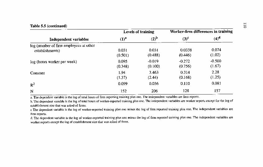
Table 5.5 (continued)
Independent variables
Levels of training(Da (2)b
Worker-firm differences in training
(3)c (4)d
log (number of firm employees at other establishments)
log (hours worker per week)
Constant
R2
N
0.031 (0.501)0.095
(0.348)1.94
(1.37)0.099
152
0.031 (0.488)-0.019 (0.100)3.463
(2.44)0.036
206
0.0338 (0.446)-0.272 (0.756)0.314
(0.168)0.110
128
0.074 (1.02)-0.500 (1.67)2.28
(1.25)0.081
157
a. The dependent variable is the log of total hours of firm-reporting training plus one. The independent variables are firm reports.
b. The dependent variable is the log of total hours of worker-reported training plus one. The independent variables are worker reports except for the log of
establishment size that was asked of firms.c The dependent variable is the log of worker-reported training plus one minus the log of firm reported training plus one. The independent variables are
firm reports.d. The dependent variable is the log of worker-reported training plus one minus the log of firm reported training plus one. The independent variables are
worker reports except the log of establishment size that was asked of firms.

On-the-Job Training 111
ing. 5 These differ greatly from the SBA and EOPP training regressions in chapter 4 in which prior experience, establishment size, and school ing were all significantly related to the amount of training. One impor tant difference is that the Upjohn Institute training measures include only training in the first month and not in the first three months. In addition, the Upjohn Institute sample sizes are much smaller, making it more difficult to find significant relationships between training and other variables.6
Columns 3 and 4 show the regressions explaining log differences in worker- and firm-reported training. There is some evidence using firm- reported characteristics that the difference between worker- and firm- reported training is negatively related to the level of schooling. No variables are significantly related to the difference in reported training when worker-reported characteristics are used.
Given the lack of any significant correlates of differences in reported training, it may be that the differences in employer- and employee- reported training result largely from measurement error. Hours of train ing may simply be difficult to estimate for the employee and the employer. If measurement error is present, then estimated effects of training on wages and productivity are biased toward zero (Greene 1993, p. 283).We investigate this issue further in chapter 6.
Conclusions
In this chapter we reported the results of a matched survey of employers and employees in which both employers and employees were interviewed three times over the course of a month. The survey focused on training activities of the last worker hired but also sought to obtain demographic information about the worker from both the firm and the worker.
There is very little difference in the quality of demographic informa tion about the worker obtained from the firm and the worker. For vari ables such as race and age, the correlations between worker and firm reports are over 0.9. Surprisingly, given that previous studies have obtained much lower correlations for wages, the correlation between worker- and firm-reported starting wages is 0.974. Lower levels of

112 How Well Do We Measure On-the-Job Training?
agreement between firm and worker reports are obtained for variables such as hours worked and union status; however, the correlations are in line with previous studies. The agreement of fringe benefits in the Upjohn Institute data are somewhat below previous estimates, perhaps because the Upjohn Institute survey focused on newly hired workers.
Correlations between worker and firm reports of training activities are in general lower than most other variables. There are no significant determinants of worker- or firm-reported total hours of training in the first month, except perhaps that those with very low schooling levels receive less training. Similarly, there are in general no significant deter minants of differences in worker- and firm-reported hours of training in the first month. A significant amount of measurement error in the worker- and/or firm-reported training variables may in part explain these findings.
There are some conclusions that can be drawn from the analysis in this chapter about whether investigators should obtain information from the firm or from the worker. For many variables, such as relevant experience, the differences in the effects of firm-reported and worker- reported variables are slight. Since the correlations for many variables are fairly high, if firm information is unavailable, it should be obtained from the worker. For example, questions about previous experience are not often asked of the worker in household surveys, but the correlation with firm-reported previous experience is quite high. Workers have much more difficulty answering questions about specific elements of the fringe benefits package. While the correlation between worker- and firm-reported training is quite low, both are significantly related to pro ductivity. It would be useful to have similar training and productivity questions appear in future household surveys.
We believe our analysis offers several insights into the measurement of on-the-job training. First, there is a great deal of measurement error in attempts to gauge the quantity of on-the-job training. Even using the aggregate measure of training, the correlation between worker and firm measures is less than 0.5, which is much lower than other variables that have been used in wage equations. Differences between firm and worker reports, however, appear uncorrelated with any of the normal variables used in wage equations. Second, firms report more training (about 25 percent more) than do workers. Heckman and Smith (1993) find evidence that workers underreport the incidence of training when

On-the-Job Training 113
comparing administrative and self-reported data for a group of Job Training Partnership Act recipients. Given our data, however, we can not determine whether this difference arises because workers underre- port training or firms overreport training (or both).
Third, both firm and worker measures indicate a large amount of informal training for newly hired workers. The incidence rate of each type of informal training exceeded 75 percent, and the mean number of hours for each type of informal training was 20 hours or more in the first four weeks of employment for both worker and firm measures. In contrast, formal training measures had relatively low incidence rates, and the mean hours of formal training in the first four weeks of training was about ten hours. This suggests that surveys such as the NLSY that focus only on formal training spells are missing a majority of the spells of training. Similarly, surveys such as the NLSHS72 and the CPS that ask retrospective questions about the informal training also appear to miss most of the spells of informal training.
Fourth, in surveys of newly hired workers, there is not much evi dence that formal training is more accurately measured than informal training. When one aggregates the five measures of training into a for mal training measure and an informal training measure, the correla tions between worker and firm measures are almost identical for formal and informal training. Fifth, firm and worker measures of the time to become fully trained and qualified, at least for our sample of newly hired workers, have lower correlations than measures of train ing. And finally, the agreement between worker and firm measures is higher for the aggregate training measure than for any individual train ing measures. This suggests that, where possible, researchers may be better served using an aggregate measure than using each measure sep arately.
Among the findings cited above, one of particular significance con cerns the size and reliability of informal training measures relative to formal training measures. The substantial magnitude of informal train ing suggests that the focus of the federal government on formal train ing may be misplaced. In fact, formal training, both as an activity to measure (e.g., the 1993 Survey of Employer-Provided Training funded by the Employment and Training Administration) and as an activity to fund (e.g., tax incentives for training personnel, instructional materials, and schools) appears less important than informal training. 7 If policy

114 How Well Do We Measure On-the-Job Training?
makers choose to subsidize formal training, they will ignore an over whelming fraction of the training that workers receive. Moreover, as we demonstrated in chapter 4, small firms are less likely to utilize for mal training than their larger counterparts. A subsidy of formal training programs, therefore, is an implicit decision to subsidize larger firms.
NOTES
1. If the establishment reported that they would be hiring in the near future, a callback was scheduled for the expected hiring date.
2. Rodgers, Brown, and Duncan (1993) and Bound, Brown, duncan, and Rodgers (1990) report correlations between log earnings. In the Upjohn data, the correlation between the logs of the employer- and employee-reported starting earnings is 0.980.
3. The correlation between the logs of the predicted wage after two years as reported by the employer and employee in the Upjohn data is 0.842.
4. We perform the Wilcoxon sign rank test and the sign test on those pairs in which the worker©s and firm©s reported disagree.
5. The worker has not asked about the establishment size so the firm-reported establishment size is used in all of the regressions reported in the paper.
6. Another important difference is that the Upjohn Institute training measure includes off-site formal training while the SBA training measure excludes off-site formal training. The SBA data report significantly different effects of off-site training from other types of training in wage and productivity equations. We find no evidence of different effects of off-site formal training using the upjohn Institute data and therefore aggregate all types of training into a single measure.
7. The 1993 Survey of Employer-Provided Training is a survey of about 12,000 employers that attempts to measure only the incidence of formal training programs.

CHAPTER
The Impact of Training on Wages and Productivity
Economists have long believed that on-the-job training is an impor tant determinant of the structure of wages. Since the seminal work of Mincer (1962), economists have attributed the growth in wages associ ated with increases in the labor market to rising productivity generated by on-the-job training. Moreover, researchers have nearly always found that wages increase with a worker©s tenure at the firm. 1 Econo mists have generally interpreted this return to tenure as evidence of firm-specific training; as noted in chapter 2, on-the-job training theory justifies such an interpretation. Consider two workers with the same years of experience in the labor market, but the first worker has been at his or her current firm for a year while the second worker has just started at a new firm. As both workers have the same total labor market experience, they should have accumulated similar general human capi tal. If the first worker has accumulated some firm-specific training, the theory of on-the-job training suggests that he or she should receive some of the returns to that training.
In the first section of this chapter, we review two theories that chal lenge the traditional training view of the source of wage growth: the incentive-based compensation models and the learning/job matching models first discussed in chapter 2. We note that, while these theories may contribute to the links between wage growth and work experience, available evidence indicates that on-the-job training remains an impor tant determinant of wage growth. However, establishing the predicted effects of on-the-job training can be difficult at times. The second sec tion of this chapter illustrates some of the difficulties in testing the pre diction that on-the-job training reduces a worker©s starting wage. In contrast, the next two sections reaffirm the predicted impact of training on wage and productivity growth, although even here questions arise
115

116 The Impact of Training on Wages and Productivity
because investments in training appear overwhelmingly to be financed by employers. We then examine the effect of measurement error on the estimated effects of training wages and productivity. The final section reviews various modifications to the simple on-the-job theory that may explain the apparent small impact of training on starting wages.
Alternative Theories of Wage Growth
There have been significant challenges to the traditional interpreta tion that employee wage growth reflects a return to on-the-job training. For instance, Lazear (1979, 1981) offers an incentive-based compensa tion model where wage profiles slope upward to guard against worker shirking. In essence, the worker posts a bond with the firm by agreeing to work for a low wage early in his or her career in return for higher wages later in the career. If workers shirk and the firm fires them, they lose the high wages or pension payments they would have otherwise received. Thus, it is possible for wages to increase with tenure without any on-the-job training. Moreover, Lazear©s theory can explain the existence of several other features of labor contracts that are difficult to explain using human capital theory. For instance, firms restrict the number of hours many employees can work. But, if firms are paying these workers the value of their marginal products or perhaps less because the workers and firms share the returns to specific training, firms should be content to let these employees work more hours. In contrast, in Lazear©s theory, firms would not want senior employees to work more hours because they are receiving a wage more than the value of their marginal products to compensate them for accepting the low initial wages.
Taking a different approach, Johnson (1978) and Jovanovic (1979a) have constructed job-matching models that may account for the corre lation of wages and job tenure. We can capture the essence of the job- matching model in a simple two-period example. Consider a model where a worker©s productivity is given by
(6.1) p/ = p + e

On-the-Job Training 117
for t = 1,2, where p° is the worker©s expected productivity across firms and e is a random variable with E(e) = 0. The term 8 is a match-specific error term that neither the firm nor worker knows before employment. During the first period, the firm and worker learn the value of e. Because £ is not initially known, a firm, competing with other firms for workers, will offer a first period wage equal to the worker©s expected productivity, or w { = p°. In the second period, however, both the worker and the firm know the true value of e. If changing jobs costs nothing, when £ < 0 it is inefficient for the match to continue because the worker©s expected productivity elsewhere is p° The worker and firm will agree to terminate the relationship, and the worker will earn the value of his or her expected productivity, or p°. If £ > 0, it is efficient for the match to continue and presumably the firm and the worker will do so. For ease of exposition, let us assume that the firm pays the worker the value of his or her marginal product, or w2 = p° + £.
In the above example, workers who change employers receive the wage /? , while workers who remain at their previous period employer receive the expected wage p° + E(e I £ > 0) > p°. Thus, seniority (ten ure) and wages are positively correlated. Yet, this in no way reflects a return to firm-specific training but rather demonstrates that good matches survive. While we may add many complications to make this example more realistic, the example does illustrate the essential insight of the job-matching literature: when good matches survive and bad matches do not, there may be a return to tenure that is a "statistical arti fact."2 While both the worker-shirking model and the job-matching model offer alternative explanations of the correlation between wages and tenure, neither theory offers a particularly compelling explanation for the correlation of labor market experience and wages. These mod els do suggest, however, that special care must be used when trying to measure the impact of training on wages.
Fortunately, there have been numerous studies that have used direct measures of on-the-job training to examine the impact of that training on wages; see Mincer (1989a) for a review. Mincer reports that even when allowing for a 15 percent depreciation rate, the returns from training range from 10.5 to 25.6 percent in the five studies that he reviews. If some of this training is firm-specific and if firms share in some of the returns to specific training, these rates of return understate the return to the economy as a whole. 3

118 The Impact of Training on Wages and Productivity
On-the-Job Training Effects on the Starting Wage
While research has typically confirmed the predicted impact of training on wage growth, the second major prediction of on-the-job training theory has proven more difficult to confirm. In fact, most pre vious research has failed to find the negative relationship between training and the starting wage predicted by this theory. Barren, Black, and Loewenstein (1989), using the EOPP data, found no statistically significant relationship between the starting wage and the quantity of training that a worker receives. As we discuss in more detail below, they argue that lack of a negative relationship between training and the starting wage may be the result of productivity differences that are not observed in the data. If high-ability workers are matched to jobs that require much training and those high-ability workers command a wage premium, there may be a spurious correlation between training and the starting wage.
Difficulties in Testing the Starting Wage Prediction Given Heterogeneous Labor
To see how heterogeneity across workers introduces difficulties in testing on-the-job training©s predictions concerning the starting wage, consider the following wage equation:
(6.2) ln(w) = X|3 + -yln(r) + a + e
where w is wages, X is a vector of firm and worker characteristics, T is the quantity of training that the worker receives, a is a measure of the worker©s ability not captured in the data, 8 are the standard error terms, and /3 and /are parameters to be estimated. If the labor market matches workers with large a's to jobs with high levels of required human capi tal, the coefficient /will be biased upward. This problem is probably unavoidable in cross-sectional data. For instance, consider a class of graduating seniors majoring in economics from the same university. From the standpoint of most standard cross-section data sets, this is a remarkably homogeneous group. They all have the same level of edu cation, their college major is the same, and they have graduated from the same university. Yet, we would hardly expect earning differences

On-the-Job Training 119
among this group to be completely random. Employers would have a wide range of information about these prospective employees that are generally unavailable to the econometrician. For instance, employers will have access to certain quantifiable measures such as grade point average, test scores, and past job earnings. In addition, employers will have access to subjective information such as workers© appearances, skills in handling interviewers© questions, personality traits, recom mendation letters, and other informal sources of information.
Despite the homogeneity of this group, we would not be surprised to learn that there are substantial earnings differentials among the gradu ates. If training and worker ability are complements in the production process so that high-ability workers have larger increases in productiv ity for a given level of training than do low-ability workers, then we would expect the "good" economics majors from the university to hold jobs that have more training than their less able classmates. Although the more able students receive more training, we still might find that they are paid a higher starting wage than the less able if the wage pre mium for their superior abilities exceeds their portion of the training costs.
To buttress the case that unobserved ability differentials may explain the lack of a negative correlation between initial wages and training, chapter 7 documents that firms look at more applicants and spend more time evaluating applicants when filling jobs that require more training. While this evidence is consistent with the lack of correlation, others disagree. Parsons (1989), using the NLS youth cohort, finds that there is a positive relationship between training and the starting wage, but the relationship is generally not statistically significant. As the NLS youth cohort is a panel data set with a much richer collection of worker characteristics (including their Armed Services Vocational Aptitude Battery scores) than the SBA and EOPP data, Parsons (1990) argues that the improved controls suggest that unobserved heterogeneity may not explain the failure of starting wages to be negatively correlated with training. Similarly, Lynch (1992), using a sample from the NLSY data of people who had attended college but did not graduate, reports that uncompleted spells of training are positively associated with the higher wages, suggesting that workers are not bearing the costs of training. While Lynch does find some differences by the level of educa tion, there is little evidence in her study that training lowers the starting

120 The Impact of Training on Wages and Productivity
wage.4 If the panel data do offer substantially more controls for worker abilities than do cross-sectional data, the failure of researchers to find a negative correlation between the starting wage and training represents a serious challenge to traditional on-the-job training theory.
A slightly more complicated model than equation (6.2) will demon strate, however, the inherent difficulty in testing this proposition, even with panel data. Suppose that the wage equation is of the form
(6.3) ln(w) = X{3 + y ln(7) + a r| + £
where a is again the worker©s unmeasured ability, r\ is a measure of the total human capital of the job, and the other variables are as before. The term 77 reflects the intrinsic human capital necessary to do the job, and, presumably, 77 is highly correlated with the quantity of training that workers receive. Of course, if we hold 77 fixed, variation in the workers© experience, schooling, and other forms of human capital will affect the quantity of training that workers receive, so r\ and training are not perfectly correlated.
Suppose that workers and firms learn about the true values of a over time. Thus, workers moving from low-training to high-training jobs (or more precisely, from low- 77 to high- 77 jobs) are more likely to be high- ability workers. If the labor market matches high ability workers to more complex jobs, then, as we discussed in chapter 2, even first "dif ferencing" the equation does not necessarily remove the bias from the estimated coefficients for
(6.4) Aln(w) = AX(3 + y ln(T) + ccAri +Ae
where A preceding the variables reflects the changes in those variables. We have assumed for convenience that the worker©s previous job required no on-the-job training. High-ability workers will tend to have larger changes in 77 than low-ability workers. As unobserved ability is positively correlated with increases in 77, and training is positively cor related with increases in 77, then the spurious correlation between train ing and the wage will not be eliminated unless we have accurate measures of 77 over the worker©s job history, which to our knowledge no panel data set contains. Workers will still have to finance their part of the training costs through accepting lower wages than firms would

On-the-Job Training 121
have paid to workers requiring less training, but the matching of high- ability workers to more complex jobs will hide the negative relation ship between training and the starting wage.
An Intrafirm Test of the Starting Wage Prediction of On-the-Job Training
Fortunately, the SBA data allow a direct test of the proposition that workers finance a part of their training cost through accepting a lower starting wage. As part of the survey, we asked whether the worker had more training, less training, or the same training as the typical worker hired into the position. In addition, we asked if the worker was paid more than, less than, or the same as the typical worker hired into the position. Human capital theory predicts that workers receiving more training than average should receive lower wages than the typical worker hired into the position, and those workers receiving less train ing than average should receive higher wages than the typical worker hired into the position. In table 6.1, we report cross tabulations for the responses to these two questions. There are several interesting observa tions. First, 21.8 percent of the sample were paid a wage higher than the typical wage whereas only 2.6 percent of the sample were paid a wage lower than the typical wage. Similarly, many more workers received less training than the typical worker (25.7 percent) than received more training than the typical worker (6.9 percent). These fig ures indicate that respondents© determination of the typical worker is biased; the worker identified as a "typical" worker is actually paid less and requires more training than the median worker. Of the small seg ment of the sample who received more training than the typical worker, more workers (16.5 percent) received wages higher than normal than received lower wages than normal (7.1 percent). Thus, there appears to be little evidence in column (1) to support the notion that workers are paying for their training when they receive more training than the typi cal worker.
When workers receive less training than the typical worker, which occurs 25.8 percent of the time, they are much more likely to receive higher than typical wages; 48.3 percent of these workers receive higher wages compared to only 12.2 percent of the workers who receive the typical amount of training. This suggests that while firms are unwilling

122 The Impact of Training on Wages and Productivity
to penalize workers who require more training than the typical new employee, they are willing to (or must) increase the wages of well- trained workers who need less training than the typical new employee. Moreover, firms© hiring decisions seem to mirror this form of rent shar ing. They are much more likely to hire workers who require less train ing than they are to hire workers who require more training than the typical new worker. As firms appear reluctant to pass the increased training costs on to workers by lowering wages, it is not surprising that they would not hire workers needing more training than the typical worker.5
Table 6.1 Training and Starting Wage, 1992 SBA Data (percent)
More Same Lesstraining training as training
than typical typical than typicalworker worker worker Total
Higher wage than typical worker (n=268)Same wage as typical worker (n=931)Lower wage than typical worker (n=32)Total3Sample size
16.5
76.5
7.1100.0
85
12.2
85.6
2.2100.0
829
48.3
49.2
2.5100.0
317
21.8
75.6
2.6100.01231
a. Totals may not add to 100 percent due to rounding.
A flaw in the above analysis is that it does not consider interfirm variation in wages and training. For instance, certain employers hiring clerks may specialize in hiring workers without much experience in the field, but they may offer these inexperienced workers a great deal of training. Other firms may only hire clerks with a great deal of experi ence who require very little training. While all workers hired at either firm may be offered the same wage, wages may differ between the firms, with the firm offering a great deal of training providing a rela tively low starting wage. This high-training firm will not be able to attract workers with a great deal of experience because of the low start ing wage. The low-training firm will offer a relatively high starting

On-the-Job Training 123
wage but may not be willing to hire workers without substantial experi ence. Thus, in the labor market as a whole, the predicted trade-off between the starting wage and training would exist, but we may not see this relationship if we look only at relative wages within the firm.
An Interfirm Test of the Starting Wage Prediction of On-the-Job Training
The prior discussion relied on firms© characterizations of a worker©s wage and training relative to the "typical" worker to test for the expected trade-off between training and the starting wage. In this sec tion, we use the 1992 SB A data set to test whether differences in train ing across firms explain differences in starting wages. The SB A survey differs from most other data sets because of its focus on newly hired workers. To help the reader compare the SB A data with other data sets, table 6.2 presents estimates of a wage equation without the measures for training but includes many of the standard controls that economists use in wage equations: age, age squared, experience, experience squared, years of education, the logarithm of the size of the establish ment, hours worked, and hours squared. In addition, we use dummy variables indicating the worker©s union status and whether the worker is black or a nonblack female. 6 The reader will recall that our measure of experience is the employer©s estimate of the number of years of rele vant experience that a worker possesses. The results offer few sur prises. Experience has a concave relationship, as do age and hours worked. More highly educated workers earn more, with one additional year of schooling increasing wages by about 10 percent. Black workers earn about 23 percent less than nonblack males, and females earn about 17 percent less than nonblack males.
In the appendix to this chapter, we provide a detailed comparison of estimates from similarly specified wage equations using the 1992 Cur rent Population Survey (CPS), the 1990 Census, and the SBA data. The estimates are similar. The largest differences are that the returns to edu cation are much higher in the SBA data and the gender gap is much smaller in the SBA data. 7 Because workers have no tenure with the firm in the SBA data, the higher return to education may reflect the fact that employers use formal education as a signal for the productivity of newly hired workers more than for a sample of workers as a whole.

124
Table 6.2 Impact of Training Proxies on the Starting Wage, 1992 SBA Data
Independent VariablesConstant
Worker©s age/ 10
Age squared / 1000
Worker©s relevant experience / 10
Experience squared / 1000
Years of education
Worker is black
Worker is nonblack female
Worker is union member
Logarithm of establishment size
Hours worked 710
Hours squared / 1000
R2
N
-0.255(1.60)0.342(3.82)-0.426(3.31)0.476(7.56)-0.933(3.72)0.100(15.75)-0.235(4.96)-0.171(6.22)0.072(1.56)0.040(5.36)0.082(1.88)-0.982(1.65)0.513
796NOTE: Absolute value of f-statistics given in parentheses. The dependent variable is the loga rithm of the starting wage. Ordinary Least Squares estimates are reported.

On-the-Job Training 125
The smaller gender wage gap is consistent with the recent findings of Wood, Corcoran, and Courant (1993). In their study of Michigan Law School graduates, they found that the gender gap was an increasing function of the time since graduation. Perhaps the largest difference, however, is that the SBA sample©s equation has an R2 over 0.51, while the R2 for the CPS is 0.36. This is not surprising, however, since wages become more dispersed as workers gain experience, and the SBA sam ple is limited to newly hired workers.
Our initial approach to estimating the impact of training on the start ing wage is to estimate equation (6.3). This requires that we not only use measures of on-the-job training but also of the total human capital of the job. After some initial experimentation with the specification using the SBA data, we decided to use two measures of training. The first measure is the sum of the intensity measures for on-site formal training, informal management, informal co-worker, and "watching others," while the second is the intensity measure of off-site formal training. We justify this separation purely on statistical grounds for we know of no theoretical reason why we should treat off-site formal training differently from other forms of training, although this has the advantage of insuring that EOPP and SBA training measures are simi larly defined.
For the correct estimation of equation (6.3), however, it is necessary to exclude measures of previously acquired on-the-job training. To see why, consider a production function for human capital. The inputs to the production function are on-the-job training acquired before employment at the firm (denoted POJT) and on-the-job training that the firm offers (denoted OJT), or
(6.5) #=/(POJT,OJT)
where/( ) is a production function with the standard properties. In fig ure 6.1, we depict two isoquants for production of total human capital, with the lower level of total human capital depicted by the curve denoted H° and the higher level of total human capital denoted Hl . These two isoquants correspond to two jobs with differing total human capital requirements. Standard human capital models would predict that a movement from point A to point B should reduce the worker©s starting wage. If we hold fixed the quantity of previously acquired on-
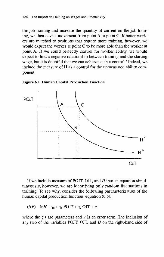
126 The Impact of Training on Wages and Productivity
the-job training and increase the quantity of current on-the-job train ing, we then have a movement from point A to point C. If better work ers are matched to positions that require more training, however, we would expect the worker at point C to be more able than the worker at point A. If we could perfectly control for worker ability, we would expect to find a negative relationship between training and the starting wage, but it is doubtful that we can achieve such a control. 8 Indeed, we include the measure of H as a control for the unmeasured ability com ponent.
Figure 6.1 Human Capital Production Function
POJT
H
OJT
If we include measure of POJT, OJT, and H into an equation simul taneously, however, we are identifying only random fluctuations in training. To see why, consider the following parameterization of the human capital production function, equation (6.5),
(6.6) In// + YO + y, POJT + y2 OJT + u
where the /s are parameters and u is an error term. The inclusion of any two of the variables POJT, OJT, and H on the right-hand side of

On-the-Job Training 127
equation (6.3) would allow, in principle, the estimation of the trade-off between training and wages. Including POJT and OJT, one can identify how, holding fixed the amount of previously acquired human capital, increases in training affect the starting wage; this is the approach of Barren, Black, and Loewenstein (1989). If markets match more able workers to jobs that require the accumulation of more human capital, however, workers at point C will be more able in observed ways than workers at point B, which will cause the coefficient on training to be biased upward.
To control for this ability bias, we propose using our measure of total human capital, the length of time it takes an untrained worker to become fully trained and qualified, as a proxy for unmeasured ability. As equation (6.6) indicates, however, the inclusion of POJT, OJT, and H into a wage equation creates some difficulty in interpretation. Hold ing constant POJT and H, movements in OJT require movements in «, unobserved factors that affect human capital accumulation. Thus, a regression so specified would not be informative. Our approach is to consider movements along the human capital isoquant such as move ments from point A to point B in figure 6.1. One can think of there being many different workers located on the locus H°. In a labor mar ket equilibrium, firms should be indifferent, ceteris paribus, between hiring workers with a lot of experience who command high starting wages and workers with limited experience who have lower starting wages.
To consider movements from point A to point B, however, it is nec essary that we allow for changes in prior on-the-job training to accom pany changes in the current employer©s on-the-job training. Labor economists use age (or potential experience, which is age minus the number of years of schooling minus six) as a substitute for general human capital, and our relevant experience is also a substitute for labor market experience. Thus, both are used as measures of prior on-the-job training. We exclude age and relevant experience from our estimation, but include our measure of H, which allows us to interpret changes in current on-the-job training as movements along the human capital iso quant.
In columns (1) through (3) of table 6.3, we report the wage equation estimates for the SB A data set using three specifications. (To avoid tak ing the logarithm of zero, we take the logarithm of one plus the training

Table 6.3 The Impact of Training on the Starting Wage, 1992 SBA and 1982 EOPP Data
Independent variablesLogarithm of job©s human capitalrequirement
Logarithm of hours of training in firstthree months
Logarithm of off-site training in firstthree months
Age and square of age addedRelevant experience and its square
addedR2
n
SBA data(Da
0.108(8.59)
-0.046(4.29)
0.024(1.91)
no
no0.442796
SBA data(2)a
0.091(7.53)
-0.035(3.39)
0.032(2.64)
yes
no0.500796
SBA data(3)a
0.077(6.91)
-0.022(2.22)
0.033(2.82)
yes
yes0.545796
EOPP data(4)b
0.053(7.18)
-0.017(2.91)
no
no0.343
1636
EOPP data(5)b
0.050(7.03)
-0.011(1.90)
yes
no0.39241636
EOPP data(6)b
0.041(5.96)
-0.004(0.81)
...
yes
yes0.4251636
NOTE: The absolute values of r-statistics are in parentheses. Dependent variables are logarithms of starting wage. Ordinary Least Squares estimates are reported.a. Other control variables are the number of years of schooling, the logarithm of the number of employees in the establishment, hours worked, the square of hours worked, and dummy variables indicating whether or not the worker is black, a nonblack female, and .a union member.b. Other control variables include years of education, a dummy variable equal to one if the worker is a female, fraction of the establishment that is union ized, the natural logarithm of the number of employees at the establishment, hours worked, hours squared, and a dummy variable indicating whether or not the worker is a temporary or seasonal employee.

On-the-Job Training 129
measures and the required human capital measure.) As mentioned ear lier, we use two measures of training. The first measure is the sum of the measures for on-site formal training, informal management train ing, informal co-worker training, and "watching others"; the second is the measure of off-site formal training. 9 In column (1) we present our preferred estimates, in column 2 we add age and age squared to the equation, and in column 3 we add relevant experience and its square to the equation. In column (1), the coefficient for the on-site training is negative (-0.046) and highly significant. A 10 percent increase in train ing decreases the starting wage by about 0.5 percent. When we add age and age squared to the equation, the coefficient on training increases from -0.046 to -0.035, and when we add relevant experience and its square, it increases to -0.022, although it remains statistically signifi cant at the 5-percent level. While the sign of the coefficient for on-site training is negative and consistent with the theory, the magnitude of the coefficient is small.
The coefficient for off-site formal training, however, is positive (0.024) and significant at the 10-percent confidence level. When we add age and its square, the coefficient increases to 0.032 and becomes significant at the five percent level, and remains significant when we add experience and its square to the equation. We tried numerous spec ification checks to see if we could eliminate the positive sign for off- site training, but none were successful. 10
In columns (4) through (6) of table 6.3, we report the estimates for the EOPP data. In column (4) our preferred specification the coeffi cient on the logarithm of training is -0.017 with a ^-statistic of -2.91. 11 Again, while highly significant, the magnitude of the coefficient is quite small. A 10 percent increase in training decreases the starting wage only 0.2 percent. If we add age and its square to the equation, the coefficient increases to -0.011, and if we add relevant experience and its square to the equation, the coefficient increases to -0.004 and ceases to be statistically significant even at the 10-percent confidence level.
For our preferred specification columns (1) and (4) the empirical tests provide mixed support for the human capital model. For both data sets, the coefficients for on-site training are negative and significant, confirming the predictions of the theory. Yet, the magnitudes of the coefficients are small, with estimated elasticities of less than -0.05. Indeed, for the SBA data, a 10 percent increase in training an

130 The Impact of Training on Wages and Productivity
increase of about 17 hours when evaluated at the mean results in a reduction in the wage of $0.04. In addition, for the SBA data, the coef ficient on off-site training is positive and significant, directly contra dicting the theory.
Some alternative measures of training provide somewhat larger esti mated elasticities. Mincer (1974), in his derivation of the earnings equations, emphasizes that the appropriate measures of training should be "the fraction of time (or ©time equivalent© if the investment costs include direct outlays as well as time costs) the worker devotes to improving his earning power" (p. 19). This suggests that the appropri ate measure of training is the intensity of training rather than the total number of hours of training received. For the SBA data, we know both the number of weeks of training and the hours per week of training that the worker receives, so we may construct a measure of the intensity of training. This allows us to construct an on-site training intensity mea sure as the total number of hours per week of on-site training and an off-site training measure as the number of hours of off-site training. Unfortunately, we cannot replicate the measure for the EOPP data set because it does not contain a measure of weekly hours of training. For the SBA data, the coefficient for on-site training intensity is -0.056 with a r-statistic of -4.05. For off-site training intensity, however, the coefficient is 0.039 with a ^-statistic of 2.33. 12
Contrasting On-the-job Training Impact on Wages Versus Productivity
While the results above support the contention that on-the-job train ing and the starting wage are negatively correlated, the magnitude of the starting wage adjustment is small. This may be due in part, how ever, to our inability to control fully for worker heterogeneity. In this section, we present a second test of human capital theory that involves a comparison of the effects of training on productivity and wage growth, a test that under certain assumptions controls for worker heter ogeneity. To see why, consider the following simple representation of the on-the-job training model developed in chapter 2.

On-the- Job Training 1 3 1
Assume that workers hired into the same position have similar unobserved abilities. Recall from chapter 2 that on-the-job training the ory predicts that, if training is general and competition exists across employers, then the starting wage and the wage paid to a fully trained worker will adjust such that for each position, the worker bears all the costs and reaps the entire return to such training. That is, the beginning wage, wb, and the wage after training, wa, are such that:
(6.7) wa =fb =p(E, a, 0, 0) - c(E, a, Tg, 0)
(6.8) wb =fa
where fb is the productivity net of training costs of a worker with initial human capital E and ability a who receives general training Tg and zero specific training, while fa is the productivity of this worker after training.
Equation (6.7) highlights the key claim of human capital theory that an increase in training T will lower the starting wage given dc/dT > 0. If positions with increased training are filled with more able individu als (i.e., dcddT > 0), and we cannot fully control for this matching of more able workers to positions with greater training, then our estimate of the negative effect of training on the starting wage will be biased upward.
Equations (6.7) and (6.8) suggest, however, an alternative test for the prediction that workers will bear the entire costs of general train ing. Specifically, dividing (6.8) by (6.7) and differentiating this expres sion with respect to a change in training, we obtain the following expression:
(6.9) d(fa /fb)/dT=d(wa /wb)/dT.
Equation (6.9) implies that the effect of general training on an index measuring productivity growth, fa/fb, and an index measuring wage growth, w/wfo , should be identical. That is, it is predicted that d (/*a//b) / dT = d(wc/wb) I dT > 0. Thus, we can restate the prediction as follows: an increase in training should result in identical increases in the growth rates of productivity and wages.

132 The Impact of Training on Wages and Productivity
Unfortunately, the SBA and EOPP data sets do not have measures of the worker©s posttraining wage. Both data sets do, however, contain measures of the wage paid to the typical worker in the same job two years after beginning employment. While there may be some jobs in which the worker is not fully trained at the end of two years, we think the wage after that time period is a good proxy for the posttraining wage. By taking the log difference of the wage paid to a typical worker in the same job after two years and the worker©s starting wage, we con struct an index of wage growth.
Table 6.4 reports the regression for the wage index. Ideally for this regression, we would like to have all the training that the worker receives in the first two years of employment, but both the EOPP and the SBA data contain only the training that the worker receives in the first three months. In column (1) we report the estimates for the SBA data. A 10 percent increase in the quantity of on-site training increases the wage growth only 0.2 percent. A 10 percent increase in off-site training decreases the wage growth 0.05 percent, although the coeffi cient is not significant. In column (3) of table 6.4, we report estimates using the EOPP data. A 10 percent increase in training increases wage growth by 0.3 percent as well. Thus, both of these coefficients suggest that increases in the quantity of training increase wage growth, and both give quantitatively similar estimates of the magnitude.
The magnitude of the trade-off, however, is not large. One would expect that a 10 percent increase in training would reduce the worker©s initial productivity by much more than 0.2 percent. Fortunately, both the EOPP and SBA data contain measures of the worker©s productivity so that we may compare the change in wages to the change in produc tivity. In the EOPP data, respondents were asked the following ques tion:
Please rate your employee on a productivity scale of zero to 100, where 100 equals the maximum productivity rating any of your employees [in this] position can attain and zero is absolutely no productivity by your employee. What is the productivity of [the last worker hired] during (his/her) first two weeks of employ ment?
We asked a slightly different version of this question to the SBA respondents. They were asked:

Table 6.4 Wage and Productivity Growth Index, 1992 SBA and 1982 EOPP Data
Independent VariablesLogarithm of training
Logarithm of off-site training
Chi-squared statistic
Wage index SBAa
(1)0.020
(4.20)-0.005(0.76)
Productivity index SBAb
(2)0.283
(10.01)0.045
(1.23)102.82
Wage index EOPP3
(3)0.028
(8.98)
...
Productivity index EOPPb
(4)0.230
(14.49)
200.02
R2 0.020 — 0.046
N________________________860_________860_________1683_________1683_____NOTE: Absolute value of t-statistics is given in the parentheses.a. The dependent variable is the difference between the logarithm of the wage paid to the typical worker after two years and the logarithm of the starting
wage of the last worker hired. Ordinary Least Squares estimates are reported.b. The dependent variable is the logarithm of one plus the index of the productivity of the fully trained worker relative to the productivity of the last worker
hired. Tobit estimates are reported.

134 The Impact of Training on Wages and Productivity
Please rate (name of last worker hired) on a productivity scale of zero to 100, where 100 equals (name©s) productivity when (he/ she) is fully trained and zero is absolutely no productivity by (name). . . . What was (name©s) productivity on this scale during his/her first two weeks of employment?
Because the reciprocals of the productivity indices are estimates of productivity growth, we may see if the impact of training on worker productivity growth is similar to the impact of training on wage growth.
In column (2) and (4) of table 6.4, we report estimates for the pro ductivity growth in the SBA and EOPP data, respectively. Because the productivity index is bounded by zero and 100, we use a tobit to esti mate the coefficients. A 10 percent increase in training in the first three months of employment decreases initial productivity by 2.3 percent in the SBA data and 1.9 percent in the EOPP data. 13 A comparison of the impact of training on starting wage indices and on the productivity indices reveals that training lowers the initial productivity of workers 11 times more for the SBA and eight times more for the EOPP data than do the starting wage indices. This suggests that workers pay for only a small portion of their training.
Indeed, in our view, it is too small a portion to be consistent with the prevailing theories of on-the-job training. While the elasticities of wage growth with respect to training are 0.02 for both data sets, the elasticities of productivity growth with respect to training are about 0.23 and 0.19 for the SBA and EOPP data. In addition, the use of a pro ductivity measure to calculate the cost of training understates the true cost of that training. Such a variable fails to account for the reduction in productivity of managers and co-workers who spend time away from their duties to train newly hired workers.
An obvious objection to this comparison questions the validity of the productivity measures. One could argue that employers are not very good about rating employees on a productivity scale. It could be that employers exaggerate the swings in productivity that new employees experience when using the productivity index. While this may be true, the underlying index values do not appear unreasonable. In table 6.5, we compare the distributions of the productivity index and a wage index for the SBA and EOPP data. The mean value of the productivity index is 51.39 percent for the SBA data and 51.01 percent for the
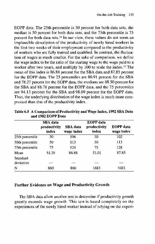
On-the-Job Training 135
EOPP data. The 25th percentile is 30 percent for both data sets, the median is 50 percent for both data sets, and the 75th percentile is 75 percent for both data sets. 14 In our view, these values do not seem an implausible description of the productivity of newly hired workers in the first two weeks of their employment compared to the productivity of workers who are fully trained and qualified. In contrast, the fluctua tion of wages is much smaller. For the sake of comparison, we define the wage index to be the ratio of the starting wage to the wage paid to a worker after two years, and multiply by 100 to scale the index. 15 The mean of this index is 86.88 percent for the SBA data and 87.85 percent for the EOPP data. The 25 percentiles are 80.91 percent for the SBA and 78.27 percent for the EOPP data, the medians are 88.50 percent for the SBA and 88.78 percent for the EOPP data, and the 75 percentiles are 94.13 percent for the SBA and 98.09 percent for the EOPP data. Thus, the underlying distribution of the wage index is much more com pressed than that of the productivity index.
Table 6.5 A Comparison of Productivity and Wage Index, 1992 SBA Data and 1982 EOPP Data
SBA data productivity
index25th percentile50th percentile75th percentileMeanStandarddeviationN
305075
51.39
860
SBA data wage index
106113124
86.88
860
EOPP data productivity
index305075
51.01
1683
EOPP data wage index
10211312887.85
1683
Further Evidence on Wage and Productivity Growth
The SBA data allow another test to determine if productivity growth greatly exceeds wage growth. This test is based completely on the experiences of the newly hired worker instead of relying on the experi-

136 The Impact of Training on Wages and Productivity
ences of the typical worker. For the SBA data, we asked about the worker©s productivity after three months of employment as well as the worker©s productivity relative to a fully trained worker. In table 6.6, we report the regression estimates for wage and productivity growth. For independent variables, we include the two measures of training: total off-site training in the first three months and total hours of other forms of training.
In columns (1) and (2) of table 6.6, we report the estimates for the wage and productivity growth equation. Interestingly, training is posi tively correlated with wage growth with an elasticity of 0.011, but off- site training is negatively associated with wage growth. Training is also positively associated with productivity growth with an elasticity of 0.190. Off-site training has no significant relationship with productiv ity growth in the first three months of employment. Thus, again, the growth in productivity greatly exceeds the growth in wages.
Table 6.6 Wage and Productivity Growth in the First 3 Months of Employment, 1992 SBA Data
Independent variables
Logarithm of training
Logarithm of off-site training R2
N
Wage growth Productivity SBAa growth SBAb
(1) (2)0.011
(3.78)-0.010 (2.58) 0.019929
0.190 (9.00)-0.005 (0.16) 0.082929
Wage growth Productivity SBAa growth SBAb
(3) (4)0.026
(3.30)-0.018 (1.59) 0.039326
0.241 (6.11)0.002
(0.38) 0.105326
NOTE: Absolute value of r-statistics is given in the parentheses. Ordinary Least Squares estimatesare reported.a. The dependent variable is the difference between the logarithm of the wage of the last workerhired after three months of employment and the logarithm of the starting wage of the last workerhired.b. The dependent variable is the difference of logarithm of the productivity index of the lastworker hired at the end of three months of employment and the logarithm of the productivityindex of the last worker hired in the first two weeks of employment.
An objection to this test is that firms may find it costly to adjust wages continuously because of what the macroeconomics literature

On-the-Job Training 137
refers to as "menu costs." The essential idea of menu costs is that price changes, or in this case wage changes, are costly to the firm. For instance, we might imagine that the decision to give a worker a raise may require the worker©s manager to meet with him or her. In addition, the worker©s manager may not have the authority to give the worker a raise and may need approval from other individuals within the firm. In addition, in many jobs workers and firms sign formal contracts that may cover a period longer than three months. For instance, each of the authors of this monograph has an annual contract that specifies his wages for a year in advance, and while none of us would object to our employers renegotiating our contract to give us a raise, we do note, sadly, that such renegotiations have not been common. 16
To guard against a bias created by any costs to changing the wage, in columns (3) and (4) we reestimate the equation on the sample of work ers who have received wage increases in that period. While the wage- training elasticity increases to 0.026, the productivity-training elastic ity increases to 0.241 and remains over nine times as great at the wage- training elasticity. Thus, again, productivity growth is much larger than wage growth. 17 Moreover, while menu costs may account for some of the lack of responsiveness of wages to productivity changes, they do not explain the whole story. Indeed, given that firms have incurred any menu costs associated with an increase in wages, we would expect this group to be free of this form of bias. If those workers who receive gen eral training are more likely to receive a raise in the first three months of employment, this group may well yield a coefficient on training that is biased upward.
The Effect of Measurement Error on the Estimated Effect of Training on Wages and Productivity?
If there is measurement error in training, the effects of training on wages and productivity are biased toward zero. One way to correct for the effects of measurement error is through the use of instrumental variables (Greene 1993). A variable must be found that is correlated with the variable that is measured with error but not correlated with the measurement error. If we assume that firm estimates of training fulfill

138 The Impact of Training on Wages and Productivity
this condition for worker-reported training and worker estimates of training do the same for firm-reported training, then we can apply instrumental variables to correct for the effects of measurement error. 18 This is similar to the approach of Ashenfelter and Krueger (1994), who use one twin©s estimate of the other twin©s schooling as an instrument for estimating the return to schooling for the other twin.
The first step in the estimation of the instrumental variables model involves estimating the variable measured with error as a function of the instrument or instruments. In this case, we use only a single instru ment the other party©s reported total hours of training. We use the training instrument for starting wage equations, wage index, and pro ductivity regressions similar to those estimated earlier in this chapter. The wage growth regressions explain the growth in starting wage to the wage of a typical worker in the same position after two years. The pro ductivity growth is the inverse of a productivity index of the new hire measured relative to the fully trained worker on a scale from 0 to 100. The productivity regressions indicate how much training increases the productivity of the new worker relative to a fully trained worker. The first stage equations for training in the first four weeks of employment are:
log(worker-reported training) = 2.09 + .414 log(firm-reported training) R2 =.156 n=179
log(firm-reported training) = 2.64 + .376 log(worker-reported training) R2 =.156 n=179
Table 6.7 shows ordinary least squares and instrumental variable estimates for starting wage, wage growth, and productivity growth regressions using the Upjohn Institute, SBA, and EOPP data sets. Using the Upjohn Institute data, the instrumental variable training esti mates are greater in absolute value than the ordinary least squares esti mates in four out of six cases. Correcting for measurement error does not appear to have a dramatic effect on the estimated training effects in the Upjohn Institute data. The estimated training effect in the firm- reported wage growth regression, however, is significant after correct ing for measurement error.

Table 6.7 Estimates of the Impact of Training on Starting Wages, and Wage and Productivity Growth
Ordinary least squaresUpjohn Institute data
log (worker-reported starting wage)3log (worker-reported wage growth)blog (worker-reported productivity growth)clog (firm-reported starting wage)alog (firm-reported wage growth)13log (firm-reported productivity growth)0
SBA datalog (starting wage)3log(wage growth)5log(productivity growth)0
EOPP datalog (starting wage)dlog(wage growth)5log(productivity growth)6
Parameter0.00310.01130.14900.01730.01000.1557
-0.0460.0200.283
-0.0190.0270.230
t0.1431.114.380.6340.874.98
4.264.20
10.01
2.968.98
14.47
n180171222158150197
796860860
1,3861,6831,683
Instrumental variables©Parameter
0.04760.00740.2259
-0.01340.12860.1854
-0.1220.0530.753
-0.0510.0720.612
t0.7600.2232.480.2063.022.18
4.264.20
10.01
2.968.98
14.47
n146138181172159207
796860860
1,3861,6831,683
a. The other independent variables used with the Upjohn Institute and SBA starting wage regressions are years of schooling; dummies for black male, black female, other male, other female, white female, and collective bargaining coverage; log of establishment size, hours of work, hours of work squared; and log of job complexity. Training is measured by the log of total hours of training plus one in the first four weeks in the Upjohn Institute regressions, and the log of total hours in the first three months plus one in the SBA regressions. The SBA regressions include off-site training as a separate variable, b. Wage growth is growth in the log of the starting wage calculated using the wage of the typical worker in the same position after two years
(continued)

c. Productivity growth is the inverse of the log of the productivity in the first two weeks of employment relative to the productivity of a fully trained worker in the same position on a scale of 0 to 100.d. The other independent variables used in the EOPP starting wage regressions are years of schooling, a female dummy variable, percent of the firm©s labor force covered by collective bargaining, log of establishment size, hours worked, hours worked squared, and log of job complexity., Training is measured by log of total hours of training plus one in the first three months (excluding off-site formal training).e. Productivity growth in the EOPP data in the inverse of the log of productivity in the first two weeks of employment relative to maximum possible pro ductivity on a scale of 0 to 100.f. Firm reported training is the instrument in the worker-reported regressions, and worker-reported training is used as the instrument in the firm-reported regressions. The Upjohn Institute worker-reported training regression estimates are combined with firm-reported training data from the SBA and EOPP data.

On-the-Job Training 141
The bottom half of table 6.7 uses the estimated regression of worker-reported training on firm-reported training from the Upjohn Institute data and the actual firm-reported training from the SBA and EOPP data to illustrate the effects of measurement error in those data sets. 19 The estimated training effects increase by almost a factor of three in absolute value in each case over the estimates reported in Barron, Berger, and Black (1993a), illustrating the effect of the measurement error on the estimated effects of training on wages and productivity.
Why is the Impact of Training on the Starting Wage so Small?
Gary Becker, in his 1992 lecture accepting the Nobel Prize for Eco nomics (1993), said, "A close relation between theory and empirical testing helps prevent both the theoretical analysis and the empirical research from becoming sterile. Empirically oriented theories encour age the development of new sources and types of data, the way human capital theory stimulated the use of survey data, especially panels. At the same time, puzzling empirical results force changes in theory" (p. 403). For both the SBA and EOPP data, we find a small impact of training on the starting wage, and an impact of training on productivity growth that is several times bigger than the impact of training on wage growth.
Are these findings consistent with theory? To be consistent, virtually all of the training must be specific and firms must bear an overwhelm ing share of the cost of training, or the returns to training must be deferred past our two year horizon by long term contracts. Fortunately, the EOPP survey asked directly about how specific their training was. The survey asked:
"How many of the skills learned by employees in this job are use ful outside of this company?1. Almost all2. Most3. Some4. Or almost none

142 The Impact of Training on Wages and Productivity
We report the responses in table 6.8. Nearly 60 percent of the sample report that the training is almost all general human capital. Only about 8 percent report that almost none of the skills are of value outside the company. Thus it appears that employees pay only a fraction of the training costs and employers feel much of that training is general train ing. We think that our findings represent one of the puzzling empirical results of which Decker speaks that need further explanation.
Currently, there are four interesting and somewhat interrelated explanations for such a finding. Parsons (1989) proposes that work ers may be unable to fund their training costs because of financing constraints. We can find some evidence for this hypothesis in the SBA data. We broke up our sample into four groups: those without a high school degree (n = 65), those whose highest grade completed was 12 (n = 313), those who attended college but did not complete four years (n = 212), and those who completed at least four years of college (n = 206). If financial constraints are important, we would expect that the coefficient on the training measure should be mono- tonically increasing in education because more highly educated work ers earn more money and, hence, should be better able to finance their training. The SBA data support this hypothesis. For high school dropouts, the coefficient on training is 0.038 with a /-statistic of 1.2; for high school graduates, the coefficient on training is -0.023 with a /-statistic of -1.6; for those with some college, the coefficient on train ing is -0.058 with a /-statistic of -2.5; and for college graduates, the coefficient on training is -0.107 with a /-statistic of -4.2.
Table 6.8 The Degree to Which Skills are General, 1982 EOPP Data
How many skills are general Fractionalmost all 59.59%mostly 13.11some 19.25almost none 8.05N = 2707_________________________100.0 ____
Unfortunately, other data are not so kind to this hypothesis. For instance, using the same four groups, we see no clear pattern in the EOPP data. For high school dropouts, the coefficient on the stock of

On-the-Job Training 143
training is -0.03 with a r-statistic of -2.0 (n = 192); for high school graduates, the coefficient on the stock of training is -0.021 with a r-sta- tistic of -2.9 (n = 960); for those with some college, the coefficient on the stock of training is -0.013 with a f-statistic of -2.1 (n = 331); for college graduates, the coefficient on the stock of training is -0.002 with a ^-statistic of -0.1 (n = 153). Lynch (1992), using data from the NLSY, divides her sample into three groups: high school dropouts, high school graduates, and those who attended but did not graduate college. She finds that the coefficient on current training spells is monotonically increasing in education, which directly contradicts the hypothesis. Indeed, of her three groups, only the coefficient for high school drop- outs is negative.
A second potential reason for the small impact of training on the starting wage focuses on the informational problem that workers and firms face. Firms have specialized in the production of their product, and presumably, they have learned a great deal about the market in which they operate. As such, these firms may know that the training they offer is general training, but convincing workers of that fact may be very difficult. Clearly, learning to use a word-processing program on a computer is general training, although many forms of training are less obvious. For instance, learning to operate a medium precision- measuring machine may facilitate learning about other pieces of elec tronic equipment. In addition, workers may find it difficult to signal their training to alternative employers. In other words, workers may believe that they are being provided with general training, but they are not convinced that they will be able to signal alternative employers of their skills.
Moreover, the extent of the market and the willingness of workers to relocate also affect the generality of training. For instance, in Scott County, Kentucky, the Toyota Motor Company has a large manufactur ing plant. Suppose that all the training that Toyota offers to their work ers is general training in the sense that it makes the workforce more productive at other automobile plants. Unfortunately for Toyota©s workers, the present worldwide excess capacity in automobile produc tion currently lessens the value of such training in the automobile mar ketplace. Should there be an increase in demand for experienced automobile workers, however, the training would be of use only to those workers who were willing to leave Scott County because there is

144 The Impact of Training on Wages and Productivity
only one automobile plant in Scott County. Thus, by forcing workers to bear the cost of training, Toyota may dissuade from applying those workers who wish to stay in Scott County for the rest of their lives. On the other hand, these may be the very workers Toyota wishes to attract.
A third possible explanation for the weak relationship between training and the starting wages focuses on the nature of labor contracts. This small literature includes Barron, Black, and Loewenstein (1993), Black and Loewenstein (1990), and Kuhn (1993). 20 Each of these papers focuses on a prevalent feature of labor contracts: they seldom specify wages for long periods into the future. Apparently, workers and firms find it efficient not to specify the wage too far into the future because of the underlying uncertainty inherent in the economy. Rather, firms and workers rely on implicit agreements, or what Okun referred to as the "invisible handshake." Such contracts allow firms and workers to respond to the changing economic climate. The flexibility associated with such contracts, however, is not without costs. Because the agree ment is implicit, it is not enforceable by third parties, and contracting parties may renege on these implicit agreements. 21
One solution to this "hold-up" problem is for contracts to be self- enforcing; that is, neither party would have any incentive to break the underlying contract once it is signed. For instance, in Barron, Black, and Loewenstein (1993) and Black and Loewenstein (1990), firms are given the right to make "take-it-or-leave-it" offers. In return for giving the firm this monopsony power, workers receive a large starting wage. In Kuhn©s paper, workers and firms play a Nash-Rubinstein bargaining game to divide the surplus. In Barron, Black, and Loewenstein (1993) and Kuhn (1993), workers who receive more specific training may receive a higher starting wage. In these models, the reason for this pre mium is that these workers have lower turnover probabilities and, hence, are more valuable to the firm. Rather than offering the workers higher initial wages, firms would ideally prefer to "backload" by offer ing to pay the workers high wages later in their career, but workers would not find such a promise credible.
Our fourth proposed explanation focuses on a broad class of models that economists call "efficiency wage" models. While this class of models is quite broad, the thread that relates these models is the notion that employers, for one reason or another, find it optimal to pay wages in excess of the market clearing wage (see Weiss 1990 for an excellent

On-the-Job Training 145
introduction to the various forms of efficiency wage models). To sim plify, we divide these models into five broad classes: effort-inducing, adverse selection, turnover-reducing, nutritional-based, and gift exchange.
In the effort-inducing efficiency wage models, with the classic refer ence being Shapiro and Stiglitz (1984), firms pay higher than market clearing wages to induce employees to work hard. If workers should choose to shirk work and risk being fired, they also risk losing the quasi-rents associated with the employment at high-wage firms. In the adverse selection version of efficiency wage models (e.g., Weiss 1980), firms offer higher wages to attract the most talented workers. If work ers know their abilities while firms imperfectly observe the abilities of workers and lower the wages paid, high-ability workers will no longer apply, but relatively low-ability workers will. Hence, reducing wages may lower worker quality. The turnover-reducing efficiency wage models (e.g., Stiglitz 1975) emphasize that firms with differing turn over costs may offer similar workers differing wages because high- turnover-cost firms will want to reduce turnover by offering relatively high wages. The nutritional-based efficiency model deals with the nutritional needs of workers and is better suited for the developing world than the ILS. economy. The last form of efficiency wages the gift exchange takes a more sociological or psychological approach. Akerlof (1982) provides the classic paper in which he argues that employees will work harder when firms provide them a "gift" of higher wages.
Efficiency wage models remain controversial; the exchange between Carmichael (1990) and Lang and Kahn (1990) offers an interesting dis cussion of the controversies. The appeal of efficiency wage models is that they provide a cogent explanation of why labor markets may not clear in the sense that the quantity of labor demanded at a given wage is not equal to the quantity of labor supplied. In our context, if labor markets do not clear, there may be no requirement that training lower the starting wage. Unfortunately, as Carmichael (1990) emphasizes, efficiency wage models have not generated a rich set of predictions that economists have subjected to rigorous empirical tests. Indeed, many of the current forms of the efficiency wage models appear inconsistent with the observed patterns of wage profiles. For instance, the shirking explanation of efficiency wages fails to explain the covariance of wage

146 The Impact of Training on Wages and Productivity
premiums across firms. While workers in positions that are difficult to monitor should receive wage premiums, workers in jobs that are easily monitored should not receive the premiums. The existing empirical work (e.g., Krueger and Summers 1988), however, suggests that wage premiums are highly correlated across occupations within industries, which suggests that monitoring costs are not driving these wage premi ums.
NOTES
1. Ransom (1993) is the exception. In his study of academic salaries, he finds that there is a negative relationship between a professor©s time at a university and the professor©s salary.
2. See Garen (1988) for a detailed review of the matching literature. The term "statistical arti fact" is from Mortensen©s (1984) working paper.
3. Altonji and Spletzer (1991); Barron, Black, and Loewenstein (1989, 1993); Booth (1993); Brown (1989); Duncan and Hoffman (1978); Lillard and Tan (1992); Loewenstein and Spletzer (1993); Lynch (1992); Mincer (1988); Parsons (1989); and Pergamit and Shack-Marquez (1987) all find that training is associated with wage growth. To our knowledge, only Veum (1993) has failed to find a positive correlation between training and wage growth.
4. In particular, Lynch finds that for high school dropouts, uncompleted spells of training are negatively correlated with wages, with a significant level of 11.6 percent two-tailed. For those with a high school degree, there is a positive correlation between uncompleted spells of training and wages, with a significance level of about 5.5 percent. For those with some college but no col lege degree, there is also a positive correlation between uncompleted spells of training and wages, which is significant at a 3.2-percent level.
5. Unfortunately, the EOPP data do not contain the same questions, so we cannot replicate these findings for that set.
6. We initially used separate gender-race controls for black, white, and other racial groups, but we could not reject the hypothesis that we could use the more parsimonious specification. See Barron, Berger, and Black (1993a) for results that use the more general specification. We also ini tially used the logarithm of the number of employees at other sites, a variable we used in our spec ification of the training equations, and we could not reject the hypothesis that its coefficient was zero.
7. Our analysis of the matched employer-employee Upjohn Institute data suggested that there may be substantial measurement error in the amount of education or workers. The SBA uses employer reports of worker education. If there is more measurement error in employer reports than in worker reports, the true gap between the SBA and the Census and CPS estimates is even wider.
8. We use ability here in a very general sense. For instance, workers with a lower turnover pro pensity would be considered "more able."
9. We tested to see if we could combine the four measures of training; the /-"-statistic was 1.11 with a p-value of 0.35. In contrast, if we try to aggregate all five measures of training, the /©©-statis tics is 7.01 with ap-value of 0.001.
10. We used specifications that included one-digit industry and occupation controls, a dummy variable indicating multiple sites, the logarithm of the number of sites, and the logarithm of the number of employees at other sites. In addition, we estimated the various permutations that arise

On-the-Job Training 147
from these three controls. Finally, we estimated the equation using the three other site controls and the one-digit industry and occupation controls. In all specifications, the coefficient was posi tive.
11. For the same of comparison with the EOPP data, we also estimated an equation using the SBA data without the measure of off-site training. The coefficient for on-site training was -0.044 with a f-statistic of -4.06.
12. A potential weakness of this measure of on-site training intensity is that it assumes all types of training are acquired simultaneously. For instance, it is possible that the workers may have types of training that begin at different times. Perhaps for the first two weeks, workers are sent to a formal training program, but for. weeks three and four, they receive informal training from their managers and co-workers. To guard against this potential bias, we define an alternative measure of training intensity as the maximum hours of any single component of training, which precludes any double counting but may understate the intensity of training. Using this alternative measure of training, the coefficient on the logarithm of training is -0.063 with a f-statistic of-4.03, while the other coefficients remain virtually unchanged. Thus, a 10 percent increase in training decreases starting wages by 0.63 percent. As another test of the robustness of the result, we define a third measure of training intensity to be the sum of the hours of all four types of training if that sum is less than or equal to the number of hours of work and equal to the number of hours of work otherwise, which may overstate the intensity of training. When we use this measure of training, the coefficient on training is -0.079 with a r-statistic of -4.49, while again the remaining coeffi cients hardly change.Using this estimate, a 10 percent increase in training lowers the starting wage by about 0.79 percent. Using these last two measures of on-site training intensity left the coefficient for off-site training virtually unchanged positive and significant at the 5-percent con fidence level.
13. One cannot interpret the coefficients from a tobit equation as derivatives. Evaluated at the means of the two samples, the derivatives are 0.8074 x P for the SBA data and 0.8238 x (3 for the EOPP data.
14. Both productivity distributions are centered at the 50th percentile and are the 75th percen- tile of both distributions are is at an index value of 75. These scores occurred without norming the productivity indices. That the medians occur exactly at 50 is probably due to the fact that employ ers are likely to pick round numbers when reporting the indices.
15. Because the literature has traditionally used the log difference in wages as an approxima tion for wage growth, we used the log difference in the starting wage and the wage after two years as an approximation of the wage index in our regression analysis. None of the results change much, however, if we use this real wage index.
16. Of course, many firms may have a probationary period and wage built into their wage pay ment structure over a fixed period of time, say three months, so wages may remain constant for other reasons than menu costs. Thus for either menu cost of account period reasons, firms may not adjust wages at the same time and rate they observe productivity growth.
17. We also estimated the wage growth equation using a tobit procedure, which resulted in a smaller coefficient on training than did restricting the sample to those with wage changes. We also ran a probit equation with the dependent variable equal to one if there was a wage change and zero otherwise. For independent variables we used the worker©s experience, logarithm of training, logarithm of off-site training, and years of education. In addition, we used the number of hours worker per week, the logarithm of the number of employees at the establishment, and a dummy variable indicating if the job was covered by a union contract. The worker©s education is negatively related to receiving a wage change in the first three months, the worker©s experience is negatively related to receiving a wage change, and each of these coefficients is significant at the 5-percent level. In addition, the coefficient on establishment size is negative with a f-statistic of -1.66. The

148 The Impact of Training on Wages and Productivity
coefficient on the logarithm of training in the first three months is positive (0.088) and statistically significant (^-statistic of 2.38). In contrast, the coefficient on the logarithm of off-site training is negative (-0.080) but has a /-statistic of only -1.70.
18. We are not assuming that the firm©s or worker©s reported training are measured without error. Rather, we are assuming that one party©s report can be used as a valid instrument for the other party©s report.
19. The SBA and EOPP data sets only asked firms about the training of the last worker hired and did not interview workers. Therefore, it is not possible to construct instruments directly from the SBA and EOPP data. Rather, one must rely on the estimates obtained from the Upjohn data. The estimated fs and standard errors remain the same because we are simply substituting a linear combination of the old variable back into the regression. Thus, these estimates are intended only to illustrate the effects of measurement error on estimated training effects. In addition, the training measures used in the SBA and EOPP data sets do not include off-site formal training. Therefore, another set of Upjohn instrumental regressions are estimated for use with the SBA and EOPP data that do not include off-site formal training.
20. Parsons (1990) also mentions problems associated with the lack of formal contracts, but he does not offer a formal model.
21. Indeed, it is often difficult to determine what that agreement actually is. For instance, IBM had a company "practice," as opposed to a "policy," of not laying off its employees. Recently, of course, IBM has fallen on hard times and has laid off some employees. Did IBM violate its implicit agreement with its employees? We conjecture that recently laid-off workers would be much more likely to say yes than the current stockholders. (That still doesn©t mean IBM violated a contract, since it was only "implicit" and not enforceable by law.)

Appendix to Chapter 6
In this appendix, we compare wage equation estimates from the SBA data with those from two commonly used micro data sets: the 1990 Census and the March 1992 Current Population Survey (CPS). For both the Census and the CPS, we limit our sample to wage and salary workers who are between 16 and 64 years of age and not full-time students. In columns (1) and (2) of table A.6.1, we report wage equation estimates where the dependent variable is the hourly wage calculated from yearly earnings for the previous year (1991 for the CPS and 1989 for the Census), the number of weeks worked, and number of hours worked per week. Both data sets contain a large number of observations, nearly 65,000 for the CPS and over 950,000 for the Census. For the independent vari ables, we include potential experience (age minus years of education minus six) and its square, years of education, a dummy variable indicating that the worker is black, a dummy variable indicating that the worker is a nonblack fe male, and hours worked per week and its square. The coefficients in columns (1) and (2) are similar except for the hours profiles, which are relatively impre cisely estimated. For comparison, we include a wage equation using similar specification with the SBA data. Several differences are apparent. First, the co efficient on education is much larger in the SBA data than in the Census or the CPS. Given that the SBA is a sample of newly hired workers, however, it is perhaps not surprising that employers reward newly hired workers more for their education than workers with some experience at the firm. Education is a readily available signal to employers that is observable at the time of hire. After employers have the opportunity to observe workers, wages may depend less on the workers© education and more on their on-the-job performance. In fact, the true magnitude of the difference may be larger than it appears if there are more problems with measurement error in employer-reported education than with worker-reported education.
There is also a dramatic difference in the coefficient on the dummy variable indicating that the worker is a nonblack female. For the SBA data, nonblack fe males earn about 19 percent less than nonblack males, while the corresponding figure for the CPS is 32 percent and is nearly 38 percent for the Census. We think this difference arises for two reasons. First, to the extent that women have higher turnover rates than men, we would expect women to have shorter tenure than men and hence the gender wage gap should be larger in a cross section of all workers than in a sample of newly hired workers. 1 Second, women are more likely to be temporary or seasonal employees than men, and temporary and part-year employees earn substantially less than permanent employees. Thus,
149

150
by using a sample of all workers rather than permanent workers, the CPS and Census will yield lower wages for women than the SB A data, which is a sample of permanent workers.
In column (4), we report a wage equation for the outgoing rotation of the March 1992 CPS. The outgoing rotation, which comprises about a quarter of the March 1992 CPS, was asked questions about their February earnings and union status. Thus, only workers who were employed in February are included in this sample. As a result, the sample size is only about 22 percent of the sam ple in column (1). By focusing on only those employed in February, we elimi nate not only the 75 percent of the sample not in the outgoing rotation but also an additional 3 percent of the sample who are not currently employed. In addi tion to using a current wage variable, this specification also includes as controls current measures of union status and firm size. Restricting our sample to these workers has a dramatic effect on the coefficient on the nonblack female vari able. The coefficient now indicates that nonblack women are paid about 22 per cent less than nonblack men. If we remove the firm size and union variables, the difference rises to 23 percent. Thus, the change in the sample is responsible for most of the change in the coefficient. Also, the coefficient on education falls, which is again consistent with the notion that education matters less for more experienced workers.
In column (5), we report the same specification of the wage equation for the SB A data. While the inclusion of the firm size and union status variables low ers the coefficient on education somewhat, it is about 50 percent higher in the SB A data than the CPS data. Similarly, for the SB A the coefficient on nonblack females is about 80 percent the magnitude of the coefficient for the CPS data. The other coefficients are reasonably similar, although the hours profile is very imprecise in the SB A data. Taken as a whole, we think this represents a reason ably similar set of estimates, especially given the differences in the samples.
NOTE
1. See Ureta (1992) for a description of the gender difference in tenure in the CPS.

Table A.6.1 Wage Equation Estimates (Ordinary Least Squares) Using the 1992 March Current Population Survey and the 1990 Census
Independent variablesConstant
Potential experience 710
Potential experience squared / 1000
Years of education
Worker is black
Worker is nonblack female
Worker is union member
Logarithm of firm size
Hours worked / 10
CPS(1)
0.667(49.70)
0.399(57.57)-0.605
(38.82)0.098
(113.37)-0.292
(34.97)-0.319
(65.10)
0.010(1.93)
Census(2)
0.607(112.55)
0.362(194.47)
-0.499(122.01)
0.093(406.98)
-0.301(134.25)
-0.375(270.31)
0.125(70.67)
SBA(3)
-0.104(0.86)0.311
(7.61)-0.563(4.58)0.133
(20.80)-0.257(5.16)-0.186(6.36)
0.103(2.29)
CPS(4)0.217
(6.33)0.282
(24.50)-0.419
(16.05)0.085
(59.04)-0.279
(19.60)-0.224
(27.22)0.137
(13.64)0.039
(19.88)0.238
(19.07)
SBA(5)-0.069(0.58)0.316
(7.86)-0.571(4.71)0.128
(19.84)-0.278(6.16)-0.178(6.16)0.070
(1.45)0.035
(4.34)0.057
(1.26)(continued)

Table A.6.1 (continued)
Independent variablesHours squared / 1000
R2
N
CPS(1)
0.004(0.31)0.26164,942
Census(2)
-0.189(99.97)
0.254950,360
SBA(3)
-0.099(1.61)0.444
796
CPS(4)-0.246
(16.41)0.360
14,244
SBA(5)-0.046(0.75)0.461
796NOTE: Absolute values of f-statistics are given in the parentheses. The dependent variables are the logarithms of wages. Ordinary Least Squares estimates are reported.

CHAPTER 7
Training and Firm Recruiting Strategies
The job-matching literature stresses that workers are not equally well suited for all positions. Rather, as noted by Topel (1986), a "heter ogeneity of talents and technologies generates job specific differences in productivity" (p. 200). Given complementarity between worker abil ity and training in production, we assumed in previous chapters that higher-ability workers are matched to positions requiring greater on- the-job training. As we have seen, because higher-ability workers com mand higher wages, the training variable in the starting wage regres sion is thus biased upward to the extent that we cannot control perfectly for ability differences among workers.
We have yet to explore the way in which high-ability workers are matched to positions with substantial training. A likely mechanism for achieving such matching is the recruiting and screening activity of employers. Employers do engage in considerable search for new work ers. For instance, using data from the second wave of the EOPP Sur vey, Barron and Bishop (1985) report that employers, on average, screen more than nine applicants before extending an offer. Moreover, Barron and Bishop (1985) document that, on average, employers spend a considerable amount of time evaluating applicants, but there is much variation in the time spent. They report that the mean time spent evalu ating applicants is about 10 hours, with a standard deviation of nearly 17.2 hours.
The issue we address in this chapter is whether the recruiting activ ity of employers, or what we refer to as employer search, is the mecha nism through which high-ability workers are matched to positions with substantial training. To examine this issue, the first section develops a model of employer search behavior in which employers obtain a noisy signal about the quality of an applicant. Considering this signal, an
153

154 Training and Firm Recruiting Strategies
employer determines whether to extend an applicant an offer or reject the applicant and continue searching. In the model, employers deter mine both their hiring standards and the accuracy of the signal that they obtain. For a fixed accuracy of a signal, the higher that employers set their hiring standards, or the greater their "reservation signal," the greater the expected ability of the worker. Higher reservation signals, however, increase the expected length of search, or require a more extensive search. For a fixed reservation signal, the greater the resources that employers devote to evaluating each applicant the greater the accuracy of the information they obtain from their search. Thus, firms face a choice of both extensive and intensive search.
The model of employer search allows us to examine how training and other characteristics of the position or applicants will affect employer search. Given that ability and on-the-job training are comple ments in production, we show that employers will adopt higher ability standards for positions requiring more training, which means that on the average they will screen more job applicants. Employers intent on matching high-ability workers to positions with more training can also raise the expected ability of a new hire by screening each applicant more intensively. By screening more intensively, an employer can raise the precision of the signals he or she obtains concerning applicants© abilities, and thus reduce the likelihood of hiring an unsuitable appli cant. Employers filling positions involving more training can therefore be expected to try to increase the ability of the new hire not only by examining more job applicants but also by engaging in more intensive, and more costly, screening of each applicant.
Predictions of the effect of training on employer search are tested using data from four national data sets: the 1980 first-wave EOPP sur vey, the 1982 second-wave EOPP survey, the 1992 SB A survey, and the 1993 Upjohn Institute survey. We find strong evidence that employ ers search more, both extensively and intensively, for positions that require substantial training. There is strong circumstantial evidence that higher-ability workers are indeed matched to positions with more training. We then consider the effect of training, as well as other vari ables, on the duration of a vacancy.

On-the-Job Training 155
Employer Optimal Search Strategy
Search by an employer to fill a vacancy can be viewed in the follow ing fashion. In each period there is the probability 8 that an applicant contacts the employer. 1 Then 1/8 denotes the expected number of peri ods between applicants. 2 The per period cost of the vacancy will be the sum of direct on-going recruiting cost as well as indirect costs reflect ing the loss of a vacancy remaining unfilled. Recall from chapter 2 that when an applicant contacts the employer, pb(E, a, 0) denotes the pro ductivity of the applicant in the absence of any training, where E denotes general human capital, a is a measure of the individuals ability level, and 0 denotes the zero vector of total acquired training, both gen eral and specific. Employers offering training during the first or begin ning period of employment incur costs c(T) reflecting the loss in productivity of the worker during training, the loss in productivity of co-workers who provide the training, and other training expenses. Thus, the net productivity of a "beginning" worker during the training period is given by:
(7.1) fb =pb(E,a,0)-c(T).
Recall from chapter 2 that if a trained worker remains with the firm, his or her productivity during the second period of employment is enhanced by the training received. That is, the productivity of a worker with ability a and education level E "after" receiving training T is given by:
(7.2) fa = Pa(E,a,T)
where 3paldT > 0 and dpjda > 0. We assume that increased ability a not only increases worker productivity, but also affects the return to training. In particular, it is assumed that oPpJdTda > 0. In words, the return to increased training is greater for more able workers (workers with a higher a).3
To introduce a rationale for employer search, we follow Jovanovic (1979b) and assume that the ability of an applicant, denoted by a, can be viewed as a random variable. We assume that the employer does not

156 Training and Firm Recruiting Strategies
know oc at the time of hire. The employer, however, incurs screening and interview costs to obtain a signal concerning the ability a of the applicant. While the signal acquired for each applicant is directly cor related with the applicant©s true ability, the signal is not perfect. Thus, some mistakes will be made in hiring. Such errors in hiring will be dis covered after a period of employment. Unfortunately, this type of learning is expensive because the employer will have already made the investment in firm-specific training.
In the above setting, the employer optimal search strategy can be viewed as making two decisions. One is to determine the minimal or "reservation signal" for acceptable applicants. An employer searches until finding an applicant with an ability signal equal to or greater than this reservation signal. Such an applicant will be offered employment. To keep our focus on employer search, we assume that any applicant who is offered employment accepts. An employer can reduce hiring mistakes by raising the reservation signal, but the cost of doing so is an increase in the expected number of applicants seen before an accept able one is found. The extent of an employer©s extensive search is reflected by this expected number of applicants seen prior to an employment offer.
The second decision of an employer©s optimal search strategy is to determine the precision of the productivity signal obtained for each applicant. By spending more time screening and interviewing each applicant, the employer can obtain a better measure of the true ability of the applicant, and thus make fewer hiring mistakes. An increase in such intensive search, however, will raise the employer©s direct search costs per applicant. Casual empiricism suggests that some employers spend a great deal of resources in trying to evaluate potential appli cants. For instance, each year corporate recruiters come to campuses across the country to interview potential employees. Generally, the recruiters ask some of the students to make a visit to the company©s plant, where more interviews are conducted. The expense of such recruiting can be quite high. Yet, employers are attempting to avoid the costs associated with hiring an ill-matched worker.
Of course, not all jobs have such a heavy investment in information before the match has begun. Fast-food restaurants do not require their employees to undergo such a rigorous selection process. Why the dif ference? Apparently, fast-food employers are more willing to wait for

On-the-Job Training 157
the information to be revealed after the employment relationship has begun. The next section considers more formally four specific factors that can help explain differences in the extent of extensive and inten sive search.
Measures of Intensive and Extensive Search
To test our theory of employer search, and in particular the effect of training on employer search, we begin by obtaining explicit measures of an employer©s intensive and extensive search choices from actual events surrounding the hiring of a new worker. Two related measures of the amount of intensive search can be constructed from the time the employer spent screening and recruiting applicants, one being the time spent per applicant and the second being the time spent per applicant interviewed. Two related measures of the amount of extensive search are also constructed. One is the number of applicants screened per employment offer, and the other is the number of applicants inter viewed per offer. Below we suggest four propositions concerning fac tors that are likely to influence these measures of intensive and extensive search.
Four Propositions Concerning Employer Search
The following four factors can affect an employer©s choice of inten sive and extensive search: the level of training (I), the dispersion in the ability distribution across applicants, the rate at which applicants arrive at the employer (<5), and the implicit cost of vacancy. Our data allow us to identify variables to proxy each of these four factors.
One key factor that influences employer search choices is the extent of training. Positions with higher training will impose larger losses on employers during the first period of employment but provide offsetting greater gains to the employment of trained workers in subsequent peri ods. The model predicts that for positions that require higher training, employers will typically increase expenditures on screening and inter viewing each applicant (greater intensive search) as well as increase the reservation signal level, leading to an increase in the expected num ber of applicants (greater extensive search). The reason is straightfor ward. Positions that require greater training offer a greater gain to

158 Training and Firm Recruiting Strategies
making fewer hiring mistakes, and both intensive and extensive search may reduce the number of mistakes. Thus, we have:
Proposition 1: Employers filling positions that require greater training will engage in greater extensive or intensive search.
Note that the reason why an increase in training may not increase both extensive and intensive search is the potential for substitution between the two types of search. For instance, an increase in training can lead to an increase in intensive search, which in turn may lower the gain to extensive search sufficiently such that the optimal level of extensive search falls. This substitution possibility is the reason for ambiguity not only here but in the next three propositions.
Naturally, factors other than training can influence employer search. A second factor that affects employer search is the inherent dispersion in the ability of workers. Leaving the mean unchanged, an increase in the dispersion of the ability distribution induces a gain to a more strin gent reservation signal. To see why, note that increased dispersion can be interpreted as an increase in the likelihood of visits by applicants with very high ability signals. Focusing first on extensive search, it fol lows that the employer faces a greater gain to continued search for such high-productivity applicants. To promote continued search, the employer raises his or her reservation ability signal. Thus, as predicted by standard search theory, the result is an increase in extensive search. As employer search occurs at both the extensive and intensive margins; however, employers have two ways of detecting the high-ability work ers. One way, just discussed, is for employers to increase the reserva tion signal level, which results in an increase in the expected number of applicants seen prior to hiring. But to better discover the high-ability applicants, the employer can also search more intensively, increasing the information content of the signal. Formally, we have:
Proposition 2: Employers filling positions for which the dispersion in ability is larger will engage in greater extensive or intensive search.
A third factor that affects employer search is the rate at which appli cants arrive at the employer (8). As an increase in the rate of flow of applicants reduces the costs of additional search, employers filling positions that have a greater applicant flow will raise the reservation productivity level, increasing the expected number of applicants. At the

On-the-Job Training 159
same time, such employers may reduce expenditures on screening and interviewing applicants, as increased extensive search substitutes for such expenditures. We thus have the following proposition:
Proposition 3: Employers filling positions where the applicant flow is greater will engage in either more extensive search or less intensive search.
A fourth factor that affects employer search is the implicit cost of hav ing a vacant position. Let us assume that sometimes an employer receives advanced notice of a vacancy. We interpret the existence of advance notice as a reduction in the cost of search to the employer because the employer can undertake the search while the current employee is still working. Such a reduction in per-period search costs increases the optimal reservation signal because the employer does not forgo the production associated with a vacant position. On the other hand, there is no clear prediction concerning the effect of such a change on intensive search. Formally, we have:
Proposition 4: When employers receive advance notice of an opening, they search more extensively, but the effect on intensive search is ambiguous.
Empirical Specification of Employer Search Equations
The above four propositions suggest five factors that affect extensive and intensive search. One is a measure of the total amount of initial training. From Proposition 1, we expect this measure of training to be directly correlated with both extensive search and intensive search, as employers increase efforts devoted to search in response to the greater loss from hiring mistakes in positions that involved greater amounts of initial training.
Proposition 2 indicates that increased productivity variation will lead to increased employer search, intensive and/or extensive. The pro ductivity of a randomly chosen applicant is a function of two factors: the applicant©s general level of human capital and his or her innate abil ity to perform the tasks required by the position of a particular employer. For workers with the same level of general human capital, the dispersion in the productivity distribution then depends on the underlying dispersion in innate abilities as well as the interaction of

160 Training and Firm Recruiting Strategies
ability and general human capital in determining productivity. If gen eral human capital and ability are complementary inputs in determin ing productivity, which is what we assume, then a given distribution of abilities will generate a more dispersed distribution of productivity among individuals with a higher level of general human capital. One measure of general human capital is formal education. This leads us to expect greater productivity variation among workers with higher levels of formal education. Thus from Proposition 2 we expect that employer search will be greater for positions that are filled by more highly edu cated individuals. A second measure of general human capital is labor force experience. Our data contain measures of whether the worker who was hired had any relevant experience for the position. We use this as a proxy for the level of general human capital gained through expe rience, and expect that the dispersion of productivity among workers with no prior experience will be less because they have less general human capital. From Proposition 2, we thus expect employer search will be less for positions hiring workers with no experience.
Another factor affecting employer search is establishment size. We take the establishment size of the employer as one measure of the rate of flow of applicants 8. In particular, we expect larger employers to experience economies of scale in generating applicants for vacant posi tions.4 Thus from Proposition 3 we expect that larger employers will engage in either more extensive or less intensive search.
Finally, from Proposition 4 we expect that when an employer has advanced notice of a vacancy, the employer will see more applicants prior to an employment offer (greater extensive search).
To summarize, the model provides the following two equations to be estimated with regard to the determinants of employers© intensive search and extensive search to fill a position:
(7.3) IS = a0 + a, TRAIN + «2 EDUC + a3 ZEROEXP + a4 SIZE + as ADVNOTICE + a6 X + e
(7.4) ES = b0 + b { TRAIN + b2 EDUC + b, ZEROEXP + b4 SIZE + b5 ADVNOTICE + b6 X +e
where IS is the log of the intensive search measure (time spent per applicant or time spent per interview), ES is the extensive search mea-

On-the-Job Training 161
sure (number who applied or the number interviewed), TRAIN is the log of the measure of total training, EDUC is the log of the number of years of education required, ZEROEXP indicates that the worker had no prior experience in a similar position, SIZE is the log of establish ment size, ADVNOTICE indicates that the employer had advance notice of the vacancy, and X is a vector of two control variables that indicate whether the position was associated with a union and the loga rithm of the number of hours the position required per week. As dis cussed above, Propositions 1 through 4 imply the following signs for the coefficients: a\ > 0 and b { > 0; a2 > 0 and b2 > 0, with strict inequal ity for at least one of the two coefficients; a3 < 0 and b3 < 0 with strict inequality for at least one of the two coefficients; a4 > 0 and b4 < 0 with strict inequality for at least one of the two coefficients; and as > 0 and no predicted sign for b5 .
The Evidence on Employer Search Behavior
To test the predictions of the model as summarized by equations (7.3) and (7.4), we employ four data sets: the 1980 EOPP employer survey, the 1982 EOPP follow-up employer survey, a 1992 survey of employers financed by the Small Business Administration (SBA), and a 1993 employer survey financed by the W. E. Upjohn Institute. Except for search variables, the contents of the first surveys have been described in detail in earlier chapters. The Upjohn Institute Survey is described in detail in chapter 7. The four surveys asked employers a number of common questions about their search activities during the period prior to their most recent hire. In particular, all four surveys contained questions regarding the number of applicants interviewed for the position filled, the number of individuals who turned the employer down, if any, and the total number of hours spent by company person nel recruiting, screening, and interviewing all applicants. We obtain a measure of intensive search by dividing the total number of hours spent recruiting, screening, and interviewing applicants by the total number of applicants interviewed.5 We obtain a measure of extensive search by dividing the total number of applicants interviewed by the total number of offers made.6 Dividing the total number of offers made by the total

162 Training and Firm Recruiting Strategies
number hired provides us with a measure of the number of offers made prior to an offer being accepted. In our discussions in the previous sec tion, we assumed this variable equaled one. Multiplying intensive search, extensive search, and the number of offers made per hire pro vides an overall measure of the total number of hours spent recruiting, screening, and interviewing applicants per hire.
Columns 1, 3, and 5 in table 7.1 report the means of these various "interview-based" measures of employer search for the four data sets. To illustrate the differences in sampling strategies across surveys, table 7.1 breaks down the magnitude of these search measures by employer size. As the table indicates, there is a substantially larger proportion of smaller employers in the two EOPP surveys relative to the SBA and Upjohn Institute surveys. After controlling for size, however, the mag nitudes of the various measures of employer search are quite similar across the four surveys, with one key exception. The total hours spent recruiting, screening, and interviewing applicants is much lower for the 1980 EOPP survey than for the other three surveys. The reason for this may be the way in which this question was framed. Unlike the other three surveys, the 1980 EOPP survey asked employers only about the number of job applicants interviewed for the position, not the total number of applicants. Thus, the answers may reflect hours involved in the interviewing process alone, not the total hours devoted to all phases of hiring for the position.
Except for the 1980 EOPP survey, the surveys also obtained infor mation on the total number of applicants for these positions. This per mits alternative measures of both intensive search and extensive search. The alternative extensive search measure is the total number of applicants seen prior to an offer, rather than the number of applicants interviewed prior to an offer. The alternative intensive search measure is the number of hours spent recruiting, screening, and interviewing applicants per applicant, rather than the number of hours spent search ing per applicant interviewed. Columns 2 and 4 of table 7.1 report means of these two variables where available.
The surveys asked employers to provide information concerning on- the-job training, although the surveys differ in the measures of training provided. The 1980 EOPP survey asked two training questions:
In the first month of employment, approximately how many hours did employees other than personnel and supervisory staff spend

Table 7.1 Employer Search, Vacancy Duration, and Training Variables by Size, 1980 EOPP; 1982 EOPP; 1992 SBA; 1993 Upjohn Institute Surveys
Number of hours spent
per Employer interview
Size (1)
EOPP, 1980 .83
1-99 .80
100-299 .96
300+ .97
EOPP, 1982 2.12
1-99 1.97
100-299 2.78
300+ 3.33
SBA, 1992 2.73
1-99 2.04
100-299 2.68
300+ 3.63
UPJOHN, 1993 3.21
1-99 1.52
100-299 3.18
300+ 3.65
Number of hours spent
per applicant
(2)NANA
NANA
2.172.142.18
2.672.11
1.882.062.431.61
1.081.761.68
Number of interviews
per offer(3)5.695.387.02
8.795.915.79
6.945.945.58
5.325.965.816.02
8.395.665.64
Number of applicants
per offer(4)NANA
NANA
9.87
8.8511.2423.42
14.089.72
13.48
19.9322.9415.68
18.8227.17
Total number of hours spent
per offer(5)
5.695.387.02
10.7510.419.36
16.5316.5014.0310.14
16.2618.4018.79
11.7518.82
20.51
Number of offers made
per hire(6)
1.021.02
1.001.021.081.071.081.16
1.141.131.16
1.141.161.46
1.211.06
Duration of vacancy in
days(7)
13.3913.46
12.0215.1317.21
16.6622.5216.67
NANANANA
30.3519.23
29.6733.41
Total training (hours)
(8)33.7132.91
37.8739.33
136.15
131.99123.30223.33
168.43152.72161.35191.0783.42
81.1
78.4086.38
Number of observations
(9)2994
2552
300142
12701083
118
69
859428102
329210
30
58122
NOTE: For comparability across the four surveys, the sample from each survey is restricted to only those who had been hired within the last two years of
the survey. The 1982 EOPP, 1992 SBA, and 1993 Upjohn Institute surveys are for the last permanent new employee hired. Information on whether the new
hire was temporary, seasonal, or permanent was not available for the 1980 EOPP survey.

164 Training and Firm Recruiting Strategies
away from their normal work routines orienting and training the new hire?
In the first month of employment, approximately how many hours did personnel and advisory staff spend orienting and train ing the new hire?
The sum of these two measures provides a direct measure of the total amount of on-the-job training, TRAIN, received by a new worker during the first month. 7 Column 8 of table 7.1 reports averages of this measure of training for the 1980 EOPP sample.
The other three surveys contained a common set of four questions concerning various types of on-the-job training, although the period of time over which training was measured differed among the three sur veys. The 1982 EOPP survey and the 1992 SB A survey asked for the total number of hours typically spent during the first three months of employment (a) by specially trained personnel providing formal train ing to the most recently hired worker, (b) by line supervisors and man agement personnel providing the new worker with informal individualized training and extra supervision, (c) by co-workers away from other tasks in providing the new worker with informal individual ized training and extra supervision, and (d) by the worker watching others perform tasks. The average total time spent on these four train ing activities, reported in column 8 of table 7.1, is 136.14 hours for the 1982 EOPP data and 168.43 hours for the SB A data. These sums pro vide direct measures of the total amount of on-the-job training, TRAIN, received by a new worker for the 1982 EOPP and 1992 SB A surveys, respectively. 8 For the 1993 Upjohn Institute survey, the train ing measure is obtained from questions almost identical to those of the 1982 EOPP and 1992 SBA surveys, with the important difference being that the training questions concern only the first month, not the first three months, of employment. That explains why the average level of training for this survey, reported in column 8 of table 7.1 as 83.42 hours, is substantially below the mean for the other two surveys.
With few exceptions, measures of the other variables included in equations (7.3) and (7.4) as determinants of employer search are avail able in all four data sets. In all four surveys, the employer provided information on the education level of the individual hired and whether the individual hired had any experience in jobs that had some applica tion to the position. We use responses to these two questions to infer

On-the-Job Training 165
the required education level of the position (EDUC) and if the employer did not require any prior experience (ZEROEXP). All four surveys also report the size of the establishment (SIZE). Three of the four surveys, the exception being the 1980 EOPP survey, contain a measure of the number of hours that the newly hired employee typi cally works. Each of the four surveys has a measure of the collective bargaining or union status of the position filled. For the two EOPP data sets, this union variable is the proportion of all positions at the estab lishment that are represented by a collective bargaining agreement. For the SBA and Upjohn data sets, this union variable is more specific; the employer identified whether the particular position filled was a union position. We control for union status because Holzer, Katz, and Krue- ger (1991), using the EOPP data, argue that queues may exist for union jobs. Only the 1982 EOPP and the 1993 Upjohn Institute surveys asked employers whether they knew in advance of the existence of the open ing.
Tables 7.2 through 7.5 report estimates of equations (7.3) and (7.4) for the 1980 EOPP data, 1982 EOPP data, the 1992 SBA data, and the 1993 Upjohn Institute data, respectively. For the intensive search equa tions (both the number of hours per applicant interviewed measure and, for the most recent three data sets, the number of hours per applicant measure), we report the standard ordinary least squares estimates with results corrected for heteroskedasticity. These results appear in col umns 1 and 2 of tables 7.2 through 7.5. Because our measure of exten sive search involves sampling from a stationary distribution with a time invariant stopping rule, the theory suggests that the average number of applicants seen per acceptable offer is exponentially distributed. 9 Therefore, the results reported in columns 3 and 4 of tables 7.2 through 7.5 reflect the estimation of a maximum-likelihood exponential distri bution (number of applicants) model using individual-level data. 10
The results reported in tables 7.2 through 7.5 provide robust evi dence supporting the employer search model we developed. Using four data sets collected over a fifteen-year period, we find strong support that employer search varies systematically by the type of position filled. Our results, summarized in table 7.6, indicate that all four data sets support the prediction that employers will search more for posi tions that require greater training, with three of the four indicating sig nificantly greater search at both the intensive and extensive margins.

Table 7.2 Determinants of Employer Search, 1980 EOPP Survey
Intensive search (IS) Extensive serach (ES)
Variable Mean
Log of number of hours spent
per interviewOLS
White (Huber) correctionCoefficient (/-statistic)
Log of number of hours spent
per applicantOLS
White (Huber) correctionCoefficient (/-statistic)
Number of interviews per offer
Exponential distributionCoefficient (/-statistic)
Number of applicants per offer
Exponential distributionCoefficient (/-statistic)
Number of offers made
per hire
Exponential distributionCoefficient (/-statistic)
Constant
Log of total training, 1st month 2.81
Log number of years education 2.48
No prior experience in position .267
Log of employer size 2.97
Advanced notice of opening NA
-.757 (3.95)
.044 (5.63)
.272 (3.55)-.077
(3.17)-.004
(0.48) NA
NA
NA
NA
NA
NA
NA
-1.40 (4.05)
.161 (11.76)
.975(7.04)-.216
(5.11).096
(7.46) NA
NA
NA
NA
NA
NA
NA
-.051 (0.15)
.002 (0.13)
.039 (0.29)-.012
(0.28)-.009
(0.67) NA

Proportion of firm unionized . 1 05
Log number of hours per week NAMean, dependent variableNumber of observationsAdjusted R-squared or Chi-square
.035(0.85)NA
.0132,994
.02
NA
NANANANA
-.131(1.89)NA5.69
2,994317.41
NA
NANANANA
-.007(0.10)NA1.02
2,994.74

Table 7.3 Determinants of Employer Search, 1982 EOPP Survey
Intensive search (IS) Extensive search (ES)
Variable Mean
Log of number of hours spent per interview
OLSWhite
(Huber) correctionCoefficient(^-statistic)
Log of number of hours spent per applicant
OLSWhite
(Huber) correctionCoefficient(^-statistic)
Number of interviews per
offer
Exponential DistributionCoefficient(^-statistic)
Number of applicants per
offer
Exponential DistributionCoefficient(^-statistic)
Constant -2.98 -3.11 -.422 .779
Number of offers made
per hire
Exponential DistributionCoefficient(^-statistic)
-.042(4.00) (3.72) (0.69) (1.19) (0.07)
Log of total training, 1st three 4.13 .117 .087 .057 .097 .005 months (7.48) (4.34) (2.92) (5.07) (0.26)Log number of years education 2.52 .716 .731 .472 .302 .023
(2.52) (2.37) (2.28) (1.40) (0.11)No prior experience in position .339 -.166 -.117 -.062 -.031 .044
(3.41) (1.91) (1.03) (0.52) (0.73)Log of employer size 3.03 .072 -.031 .053 .211 .007
(4.06) (1.35) (2.53) (10.02) (0.33)Advanced notice of opening .60 .133 -.019 .180 .335 -.014
(2.80) (0.33) (3.09) (5.72) (0.24)

Proportion of firm unionized .098
Log number of hours per week 3.60
Mean, depend, variableNumber of observationsAdjusted R-squared or Chi-square
.005(0.05)
.239(3.12)
.4091,294.11
-.268(2.01)
.393(3.58)
.3411,294.05
-.180(1.64)
.146(1.34)5.911,270
43.12
.119(1.06)
-.160(1.46)9.861,270
213.68
-.067(0.61)
.005(0.05)1.081,2701.15
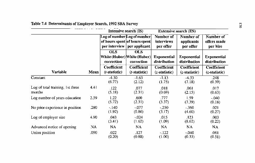
Table 7.4 Determinants of Employer Search, 1992 SBA Survey
Intensive search (IS) Extensive search (ES)
Variable Mean
Log of number of hours spent per interview
OLS White (Huber)
correctionCoefficient (^-statistic)
Log of number of hours spent per applicant
OLSWhite (Huber)
correctionCoefficient (^-statistic)
Number of interviews per offer
Exponential distributionCoefficient (z-statistic)
Number of applicants per offer
Exponential distributionCoefficient (z-statistic)
Number of offers made
per hire
Exponential distributionCoefficient (z-statistic)
Constant -4.30 -1.63 -1.13 -4.33 .248 (6.77) (2.12) (1.75) (7.18) (0.39)
Log of total training, 1st threemonthsLog number of years education
No prior experience in position
Log of employer size
Advanced notice of opening Union position
4.41
2.59
.280
4.90
NA.090
.122 (5.18)1.22
(5.72)-.140 (1.92).043
(3.41)NA.022
(0.20)
.077 (2.31).600
(2.31)-.077 (0.86)-.024 (1.62)NA.127
(0.88)
.018 (0.69).777
(3.37)-.250 (3.17).015
(1.09)NA
-.122 (1.00)
.061 (2.15)1.59
(7.39)-.360 (4.60).123
(8.62)NA
-.040 (0.33)
.017 (0.63)-.040 (0.18).021
(0.27).003
(0.22)NA.061
(0.51)

3.54 .272 .034 .209 .545 -.033(2.79) (0.33) (2.18) (5.79) (0.36)
Mean, dependent variable .545 .248 5.58 14.08 1.14Number of observations 859 859 859 859 859R-square or Chi-square .14 .02 42.53 267.58 1.01

Table 7.5 Determinants of Employer Search, 1993 Upjohn Institute Survey
Intensive search (IS) Extensive search (ES)
Dependent variable:
Model estimated
Variable Mean
Log of number of hours spent
per interviewOLS
White (Huber) correctionCoefficient (^-statistic)
Log of number of
hours spent per applicant
OLS White (Huber)
correctionCoefficient (^-statistic)
Number of interviews
per offer
Exponential distributionCoefficient (z-statistic)
Number of applicants
per offer
Exponential distributionCoefficient (z-statistic)
Number of offers made
per hire
Exponential distributionCoefficient (z-statistic)
Constant
Log of total training, 1st month 4.05
Log number of years education 2.61
No prior experience in position .148
Log of employer size 6.14
Advanced notice of opening .743
Union position .100
-5.91 (4.68).108
(1.79)1.86
(4.14)-.207 (1.37).045
(1.19).029
(0.23)-.114 (0.59)
-2.98 (2.02).044
(0.58)1.30
(2.54).129
(0.61)-.009 (0.18)-.119 (0.61)-.459 (1.85)
-0.99(0.72).135
(1.93).607
(1.29)-.391 (1.94)-.077 (1.83).197
(1.21)-.052 (0.22)
-6.47 (4.35).132
(1.87)1.96
(3.86)-.834 (3.86).037
(0.85).618
(3.75).292
(1.99)
.651 (0.47)-.022 (0.30)-.254 (0.52)-.067 (0.34)-.043 (0.95).006
(0.03).009
(0.04)

Log number of hours per week 3.57 .312 -.119 .283 .890 .145(2.11) (0.61) (1.29) (4.02) (0.68)
Mean, depend, variable .733 .000 6.02 22.94 1.16Number of observations 210 210 210 210 210R-squared or Chi-square .17 .04 17.81 79.59 1.96
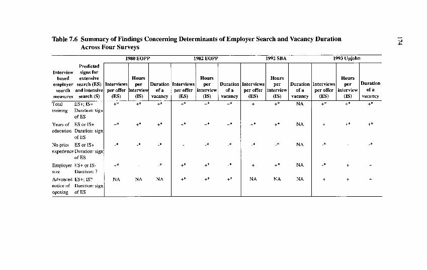
Table 7.6 Summary of Findings Concerning Determinants of Employer Search and Vacancy Duration Across Four Surveys
1980 EOPP 1982 EOPP 1992 SBA 1993 Upjohn
PredictedInterview signs for
based extensive employer search (ES)
search and intensive measures search (S)
Total ES+; IS+training Duration: sign
ofES
Years of ES or IS+education Duration: sign
ofES
No prior ES or IS+ experience Duration: sign
ofES
Employer ES+ or IS- size Duration: ?
Advanced ES+; IS?notice of Duration: sign opening of ES
Interviews per offer
(ES)+*
+*
.*
+*
NA
Hours per
interview(IS)
Duration of a
vacancy
+* +*
+* +*
.* .*
.*
NA NA
Hours Interviews per per offer interview
(ES) (IS)
Duration of a
vacancy
+* +* +*
+* +* +*
.* -*
+* +* -*
+* +* +*
Hours Interviews per per offer interview
(ES) (IS)+ +*
+* +*
.* .*
+ +*
NA NA
Duration of a
vacancyNA
NA
NA
NA
NA
Hours Interviews per Duration per offer interview of a
(ES) (IS) vacancy+* +* +*
+ +* +*
.* . .*
-* + +
+ + +

Applicantbased
employersearch
measures
Total ES+; IS+training Duration: sign
ofES
Years of ES or IS+education Duration: sign
ofES
No prior ES or IS+experience Duration: sign
ofES
Employer ES+ or IS-size Duration: ?
Advanced ES+; IS ?notice of Duration: signopening of ES
Applicantsper offer
(ES)
NA
NA
NA
NA
NA
Hoursper
applicant
NA
NA
NA
NA
NA
Applicantsper offer
(ES)+*
+
-
+*
+*
Hours perapplicant
+*
+*
.*
-
.
Applicantsper offer
(ES)+*
+*
.*
+*
NA
Hours perapplicant
+*
+*
-
_*
NA
Applicantsper offer Hours per
(ES) applicant
+* +*
+* +*
_*
+
+*
NOTE: An asterisk indicates the coefficient is significantly different from zero at the .10 significance level. Pluses and minuses indicate the sign of the coefficient.

176 Training and Firm Recruiting Strategies
There is similarly strong support for the prediction that employers search more extensively for positions that require greater levels of edu cation. 11 Further, all four data sets provide at least partial support for the contention that employers search less on the extensive margin for positions that do not require prior experience, and three of the four data sets support the contention that larger employers search more at the extensive margin. On the other hand, there is no strong evidence that larger employers search less intensively. Estimates of equations (7.3) and (7.4) that include the advance notice variable for the 1982 EOPP and 1993 Upjohn Institute data sets indicate, as expected, that while advance notice has an indeterminate sign with respect to intensive search, the advance notice of a vacancy does lead to an increase in extensive search.
There is an additional finding from the four surveys that is of inter est. Column 5 in tables 7.2 through 7.5 reports the estimation of a sur vival model for the number of offers made per hire. All four surveys indicate that it is uncommon for applicants to reject wage offers (see column 6 of table 7.1): in all four data sets, workers accept at least 85 percent of all job offers. Further, there is no systematic pattern to the rejection of wage offers across positions.
The Evidence on Vacancy Duration
The analysis in the previous section provides not only a framework for the analysis of factors affecting employer intensive and extensive search, but also suggests determinants of the duration of a vacancy. The model specifies that the duration of a vacancy is an exponentially dis tributed random variable with expected value 1 /(8(l - H(sr)), where 8 is the per-period probability that an applicant will contact the employer seeking to hire and (l-H(sr)) is the probability that an applicant is acceptable given the distribution of ability signals //( ) and reservation signal sr Thus, the expected duration of a vacancy is an increasing function of the employer©s reservation ability signal choice, sn and a decreasing function of the probability that an applicant contacts the employer, 8.

On-the-Job Training 177
This implies the hazard rate function for vacancy duration is time independent. 12 In this case, letting D denote the log of the duration time for a vacancy, the model we estimate is given by:
(7.5) D = c0 + c, TRAIN + c2 EDUC + c3 ZEROEXP + c4 SIZE + cs ADVNOTICE + c6 X + e
where the predicted signs for the coefficients in equation (7.3) are the same as those for the extensive search equation (7.4), with one excep tion. The exception is the employer size variable. Recall that while larger employers are predicted to search more extensively (higher sr), the rationale for this is that larger employers have a greater probability of an applicant contact each period (a higher 8). These two changes (higher sr and higher 8) have offsetting effects on the duration of a vacancy. Thus, the effect of size on the duration of a vacancy is ambig uous. Given that we have found that extensive search increases with training, education, and advance notice, and decreases in positions that require no prior experience, then these variables should have similar effects on the duration of a vacancy.
Because the data are measured in days and the number of observa tions in our data sets are relatively large, we treat the data as discrete. 13 While our theory implies that the hazard function should be time invariant, van Ours (1988) and Renes (1989) report evidence of dura tion dependence. To check this result for U.S. data, we estimate the vacancy duration model using a discrete hazard model that Kalbfleisch and Prentice (1973) suggest. Meyer (1990) recently applied this model to unemployment spells. Let the duration time have a discrete distribu tion with mass points at 0 < z\ < Z2 • • •• Then the Kalbfleisch and Pren tice model implies the hazard at zt for covariate x is:
(7.6) l-(l-yt)exPt-* c i
where yt and the coefficient vector C are parameters estimated using maximum likelihood techniques. 14 The discrete, time-invariant hazard function is 1 - ( 1 - ^)exp[-*c] ? wm"ch is simply a special case of equa tion (7.6). We estimated both models for each of the three data sets that contain information on the duration of the vacancy and overwhelm-

178 Training and Firm Recruiting Strategies
ingly reject the constant hazard function specification for each of the three data sets.
For the 1982 EOPP and 1993 Upjohn data sets, the duration of a vacancy is measured by the number of days "between the time (the employer) started looking for someone to fill the opening and the time (a new employee) started to work." For the 1980 EOPP, the term "recruit for the job" was used instead of "looking for someone to fill the opening." 15 Columns 1 through 3 of table 7.7 report the results of this estimation of the vacancy duration equation. The estimated hazard rates for the three separate data sets are plotted in figure 7.1. There is some evidence of time dependence. For instance, one pattern indicated by figure 7.1 is that the probability of filling a vacancy rises at the end of the first week. It appears that a common event is for an employer to fill a vacancy after a week of search. A second pattern, apparent in the
Figure 7.1 Vacancy Duration Hazard Rates (duration in days)
•EOPP 1982 — - — - Upjohn 1993\
two EOPP data sets, is a relatively high likelihood of a vacancy being immediately filled. These are positions for which the employer either indicated that there were no days between the time he or she started to look for someone to fill the opening and the time that the new employee started to work or that he or she did not have to look for someone to fill the position. One reason that the immediate filling of vacancies does not occur in the Upjohn Institute data set is that firms who fill positions immediately tend to be smaller employers, and

Table 7.7 Vacancy Duration Models1980
EOPPCoefficient
Variable (z-statistic)
1982EOPP
Coefficient(z-statistic)
1993Upjohn
Coefficient(z-statistic)
Duation(in days)
1980EOPP
Estimatedhazard rates3
1982EOPP
Estimatedhazard rates3
1993Upjohn
Estimatedhazard rates3
Log of total training 1 st three months(1st month for EOPP 1980)
Log number of years education
No prior experience in position
Log of employer size
Advanced notice of opening
Proportion of firm unionized (unionposition for Upjohn 1993)
Log number of hours per week
Median of dependent variable (indays)Number of observationsLog likelihood
.112(8.33)
.574(4.32)
-.201(4.71)
.004(0.34)NA
-.015(0.22)NA
142,994
-6400.09
.108(5.32)
.886(4.88)
-.111(1.79)-0.16(0.79)
.259(4.38)
-.206(1.81)
.490(4.77)
141,270
-2794.35
.141(1.78)2.432
(4.50)-0.888(4.01)
.003(0.68)
.281(1.59)
.429(1.65)
.491(2.26)
22210
-394.94
0
1
2
3
4
5-7
8-14
15-2122-3031-6061-90
0.2706
0.1005
0.0829
0.0662
0.0235
0.1054
0.0685
0.03530.04940.01340.0107
0.1243
0.0528
0.0551
0.0700
0.0324
0.1013
0.0691
0.03840.05120.01720.0110
...
0.0039
0.0120
0.0163
0.0125
0.0261
0.0179
0.04050.03800.02470.0213
a. We calculate hazard rates using the mean value of the covariates for each sample.

180 Training and Firm Recruiting Strategies
smaller employers were specifically excluded from the Upjohn Insti tute sample. Our findings generally support the presumption that changes in variables that lead to more extensive search are the same changes that lead to an increase in the duration of a vacancy. The one exception, employer size, supports our conjecture that it should have different effects on extensive search and vacancy duration. While larger employers do search more extensively, the expected duration of a vacancy is equal to or less than that of smaller employers.
Recently, van Ours (1988) and Renes (1989), using Dutch data, explored the determinants of vacancy duration. They found that vacancy duration was higher at positions with high education, experi ence, and skill requirements. Our findings for the United States across three data sets are consistent with these findings: we find that vacancy duration is significantly greater in positions requiring more training, more highly educated workers, and individuals with some prior experi ence. Our findings, however, indicate a much shorter duration of a vacancy than that found in the Dutch data. From table 7.1, mean vacancy duration is under a month, while the average vacancy duration for the Dutch data was about six months. Some of this difference may be explained by the fact that the Dutch data was drawn by sampling vacancies, then resampling the employers later to determine the time taken to fill that particular vacancy. Such a sampling strategy overrep- resents positions that have long vacancy durations. More in line with our data are Scottish data reported by Beaumont (1978), who found an average vacancy duration of between 10 and 15 days during the 1973- 1975 period.
Conclusions
While much has been written concerning job search, researchers have placed less attention on employer search. This appears odd given our results, which confirm that systematic patterns to employer search do exist and that employer search is an important component of the matching of workers to positions. Table 7.8 indicates that the median duration of unemployment is substantially higher for workers in mana gerial and professional occupations, occupations that typically require

On-the-Job Training 181
higher levels of education and more training than service occupations. Our finding that employers search more extensively for positions that require greater formal education and training may help explain this dif ference in unemployment duration. More extensive search by employ ers means that workers must on average locate more vacancies per job offer. Our results on extensive search by employers are also consistent with Holzer©s (1994) finding that positions involving greater job skill requirements generally have higher vacancy rates. That we find that employers search more extensively to fill such positions (with a result ing longer duration of a vacancy at these positions) implies higher vacancy rates, other things equal.
Table 7.8 Employer Search and Unemployment DurationMedian duration Mean number of
(weeks) of applicants perOccupation unemployment3 offer (SBA)
Service 7.3 7.7Operators, fabricators, and laborersTechnical, sales, aridadministrative supportPrecision production, craft, and repairManagerial and professional
9.0
10.112.212.6
12.9
14.814.518.7
a. As the duration of unemployment data is censored, we report the median rather than the mean of the interrupted duration spells as it is likely to provide a better measure of the underlying mean duration of completed spells of unemployment. Employer extensive search is measured by the mean number of applicants seen per offer reported by the Spring 1992 SBA survey. The median duration of unemployment is taken from the June 1992 issue of Employment and Earnings and for the month of May 1992.
One important extension of our analysis would be to consider fur ther the interplay between employer search decisions and worker job search. For instance, as Montgomery (1991) emphasizes, if workers know the search behavior of employers, then employers who make rel atively few offers per applicant will have to pay higher wages to com pensate applicants engaged in costly job search for the reduced likelihood of receiving a job offer. Another issue that warrants further examination is the implication of employer search for the sharing of on-the-job training costs and returns. We assumed for simplicity that

182 Training and Firm Recruiting Strategies
employers bear all the costs and reap all the returns to training. In a more general setting, however, the employer©s share of training cost should be endogenously determined, with the employer bearing a larger portion of training costs and returns at positions requiring sub stantial training in order to induce a more careful matching of workers and positions (e.g., to induce the appropriate investment in employer search). This provides an additional rationale for the findings in chap ter 5 of a weak relationship between starting wages and training.
NOTES
1. In modeling employer search, there are several options available. The simplest approach, which is the one we adopt, assumes a sequential strategy. This is standard in the literature that examines search from the worker©s point of view. There are, however, situations in which the opti mal search strategy combines elements of the fixed-sample-size approach with the sequential approach. The optimality of a search strategy that includes a. fixed-sample-size element is demon strated by Morgan and Manning (1985). For instance if there is a delay between the interviewing of an additional worker and the decision to hire, the fixed-sample-size element of search increases the speed at which the vacancy can be filled. Naturally, offsetting this gain is the potential of a fixed-sample-size strategy to result in an overinvestment in information. Bull, Ornati, and Tedes- chi (1987) provide an illustration of an employer who chooses a combined fixed-sample-size/ sequential search strategy. Employers do, in fact, often engage in search strategies that combine fixed-sample-size properties with sequential strategy. The added complexity of such a model of employer search, however, is not required to illustrate the interplay between belated information and employer search and to identify how factors such as the extent of on-the-job training influence employer search.
2. For simplicity, we assume the length of a period is sufficiently short such that the probabil ity that two or more applicants contact the employer in the same period is approximately zero. We also choose not to complicate the model by having the employer choose the extent of (costly) advertising that would affect the speed at which applicants visit the employer. As noted by van Ours and Ridder (1992), such advertising can be the source of a pool of applicants.
3. We could also assume that higher-ability workers have lower costs of training. In other words, we could assume that 32c/3T8cc < 0, such that the reduction in output during the first period that results from an increase in training is less for higher-ability workers. The results to follow would not be affected by adding this feature to the model.
4. These economies of scale may arise in part due to the existence of personnel departments that increase the flow of applicants per vacant position, van Ours and Ridder (1992) do find that ". . . establishments with a personnel department. . . have more applicants" (p. 149).
5. Recall that the extent of intensive search excludes the indirect costs of a vacancy remaining unfilled. As this intensive search measure is computed by dividing the total time spent searching by the number interviewed, we add one to the number interviewed as reported by the employer in order that all employers, including those who reported interviewing zero individuals prior to hir ing, are included in the analysis. Except for the 1980 EOPP data, the number reporting no inter views was under 10 percent. For the 1980 EOPP data set, approximately 30 percent of employers reported no one was interviewed. This large number may be due in part to the absence of a preced ing framing question concerning the number of applicants for the position.

On-the-Job Training 183
6. Given that we add one to the reported measures of the number interviewed to compute the intensive search measure, we add one to the number interviewed in computing the extensive search measure, such that the product of these intensive and extensive measures equals total search. Estimation of a survival model for extensive search also requires that the lower bound for the number interviewed must be above zero.
7. This training measure is clearly truncated as the training refers only to the first month of employment. The substantially greater estimates of training over the first three months of employ ment reported below for the 1982 EOPP and the 1992 SB A illustrate this point.
8. The fourth measure of training was in response to the question concerning the total hours spent by the worker "in training activities in which he or she is watching other people do the job rather than doing it himself (EOPP data set) or "observing co-workers in order to learn skills required for the position" (SBA data set). One might omit this variable from our total training measures on the presumption that it introduces some double-counting given our other three train ing measures. The deletion of this fourth training variable, however, does not alter any of the find ings reported below.
9. Thus, our measure of extensive search has features similar to duration data.10. The significance of the reported results are robust to alternative estimation procedures. For
instance, estimation of the model using Davidon, Fletcher, and Powell (DFP) algorithm provides identical coefficients and similar estimates of the standard errors. We also used robust confidence standard errors of Huber (1967) and White (1980) in the exponential models and our findings largely unchanged.
11. van Ours and Ridder (1992) have a similar empirical finding that employers see more applicants prior to hire at positions requiring higher educational levels.
12. In general, the vacancy duration hazard rate function ht is the probability that a vacancy is filled at any given instant /. Time (duration) independence means that dX, Idt = 0 for all t, and occurs if the distribution of vacancy duration is exponential.
13. See Kalbfleisch and Prentice (1980) for a good discussion of the estimation of discrete hazard models.
14. We follow Kalbfleisch and Prentice©s (1980) suggestion and use the Kaplan-Meier esti mates of the empirical hazard functions for the starting values of the y©s and C = 0. When C = 0, the method of Kalbfleisch and Prentice yields Kaplan-Meier estimates for the hazard function. Cox also proposes a discrete hazard model; if we adopt his approach, the parameter estimates for the C©s and the estimates of the hazard function are very similar to the estimates produced by the method of Kalbfleisch and Prentice.
15. Holzer (1993a, 1994) and Holzer and Montgomery (1993) analyze the 1980 and 1982 EOPP data on firm vacancy rates, but do not examine the data on the duration of vacancy for the last worker hired by these firms. Holzer©s (1994) finding concerning the factors that affect vacancy rates complements our findings concerning factors affecting employer extensive search and thus the duration of a vacancy.
16. By other things equal, we mean the following. Let P, denote the number of positions of type / and let £, denote the number employed in type i positions, such that the number of vacan cies is Pj - EJ and the vacancy rate for type / positions is given by v(- = (/*,- - £,)/£,. Assume a con stant exit rate q from the employed ranks that is the same across all types of positions. Then for type i positions, qEt denotes new vacancies created each period. In the steady state, the number of vacancies for positions of type i that are filled equals qEj, the likelihood that a vacancy is filled is qEj/(Pj - EJ), and the expected duration of a vacancy for a type i position is given by £>, = !%£,-/ (Pi - £,-)) = Vj/q. Thus, the steady-state vacancy rate for positions of type i equals the common rate at which employed positions are vacated times the expected duration of a vacancy for positions of type i.


CHAPTER 8
ConclusionsWhat have we learned about training from the EOPP, SBA, and
Upjohn Institute data sets? First, all the data sets agree that nearly all newly hired workers undergo on-the-job training. Moreover, in the first three months of employment, both the EOPP and SBA data suggest that newly hired workers, their co-workers, and their supervisors spend the equivalent of nearly four 40-hour weeks in training. Several other surveys, however, demonstrate much lower incidence rates of training, even if the sample is restricted to newly hired workers. But, when newly hired employees and their employers are asked a similar set of questions about training, both groups agree that training is nearly uni versal. This correspondence suggests that researchers must carefully design surveys to capture fully the types and quantities of training that workers receive.
The data also indicate that college-educated workers and workers employed in large establishments receive more training than other workers. College-educated workers have shown a proficiency for accu mulating human capital during schooling, and this proficiency appar ently extends to the workplace. Presumably, large establishments find training less costly than smaller establishments. Large firms can spread any fixed costs associated with training over their larger number of new hires, and they are more able to have co-workers provide the training without experiencing significant productivity losses.
The EOPP, SBA, and Upjohn Institute data sets also show that train ing generates productivity growth. In the absence of explicit measures of productivity, we relied on a subjective measure in which the employer rates the new employee against a fully trained employee. The productivity index demonstrates that training results in substantial pro ductivity growth: a 10 percent increase in training raises productivity 2 percent during the first three months of employment.
185

186 Conclusions
On-the-job training also increases wage growth. Whether looking at wage growth in the first three months or first two years of employment, the data indicate significant increases in wages associated with train ing. These findings confirm the predicted effects of on-the-job training on wage and productivity growth. The magnitude of the wage growth effect, however, suggests that current theories of on-the-job training are not satisfactory. A 10 percent increase in training results in only about a 0.2 percent growth in wages, or about one-tenth the magnitude of the impact of training on productivity growth. Such a differential could, with some difficulty, be justified if all training were firm-spe cific, but the impact of previous experience on wages makes it difficult to accept this proposition.
Further problems arise when trying to confirm the prediction that on-the-job training decreases the starting wage because workers bear at least some of the costs of training. We do find some evidence that train ing lowers the starting wage; a 10 percent increase in training in the first three months of employment lowers the starting wage between - 0.5 and -0.2 percent. Workers appear to bear little of the training costs while firms bear most of the costs. Moreover, whether we infer the fraction of the training that is general training indirectly from the observed effect of previous experience on wages or directly from responses to survey questions, most of this training appears to be gen eral training. The notion of firms bearing the costs of general training is inconsistent with any equilibrium model of labor markets of which we are aware.
If firms do bear a large portion of training costs, hiring the wrong worker for a job requiring a significant amount of training is a very costly mistake. Firms should be willing, therefore, to expend resources to avoid these mistakes by improving their recruiting when hiring for such positions. As we demonstrated in chapter 7, firms recruit more intensively (they spend more time with each applicant) and more extensively (they see more applicants per position) when recruiting for positions with more training. To the extent that this increased effort results in higher-quality workers, the firm matches higher-quality workers to positions that require more training. As higher-quality workers command higher wages, this finding helps explain why posi tions with substantial training do not have significantly lower starting wages.

On-the-Job Training 187
Perhaps our most important findings come through the use of the Upjohn Institute survey that matched responses of employer and employees to a set of identical questions. We found significant differ ences in employer and employee reports across human capital mea sures, including both schooling and training measures. Training measures had correlation coefficients between employer and employee reports of only 0.2 to 0.4 for the individual measures and only about 0.5 for the aggregate measure. For education, the correlations are somewhat higher, especially at the higher levels of educational attain ment, but there are substantial differences in employer and employee reports. Future research, therefore, must be concerned with the quality of the data used in attempting to measure the impact of human capital on wages.
For many years now, the wages of the least-educated Americans have declined while the wages of the most-educated Americans have increased. For instance, Katz and Murphy (1992) report that the earn ings of high school dropouts between 1979 and 1987 declined 6.6 per cent, while the earnings of college graduates increased 7.7 percent in the same period. 1 At least in part, these changes have created renewed interest in "investing in people" and mobilized policy makers to act on the perceived lack of investment in human capital. (So pervasive is this view that James Heckman (1993) refers to it as the "new consensus.") What insights do our findings provide concerning the forthcoming debates over how to increase the human capital of lower-income work ers?
First, for policy makers who wish to argue that the market under- provides training opportunities for workers, our results offer some evi dence for this view. Firms appear to finance a large amount of general training. While there may be other distortions that counterbalance the incentive to under-provide training, it seems unlikely, in our view, that such counterbalances would ever result in firms providing too much training. Thus, government may have an additional role to play in the human capital market.
Government already provides massive subsidies to education, and we may have too much schooling relative to job training in our human capital production. If policy makers wish to pursue policies that increase job training, our results also provide some insights into which policies may be effective. Most important, our results indicate that pol-

188 Conclusions
icy makers should not overlook the importance of informal training in the acquisition of job skills. By far the majority of employee training for all sizes of establishments, and especially for smaller establish ments, is informal. Because workers and firms agree to provide this training voluntarily, we believe they do so because they find it efficient. Informal training is a less costly way of imparting human capital than formal training programs for the acquisitions of many types of skills. Because human capital should be produced as efficiently as possible, we should not encourage more expensive methods of imparting human capital through policies that emphasize formal training. Policies should not ignore the role of informal training.
For instance, suppose that you were concerned about the dismal level of training among academic economists. You mandate that uni versities and colleges spend 5 percent of the wage bill of their econom ics departments for training of economists. We predict you would soon find that there would be large training conferences in Honolulu in the middle of winter. Among the expensive flights, the expensive hotels, luaus, and mai tais, some useful training will occur, but this "training" is clearly less efficient than the economists going into their offices on a Saturday and, informally, learning some additional economics. (If this scenario sounds fanciful, examine how medical doctors meet their con tinuing education requirements, or where other professions have their trade meetings.)
Inducing substitution from inexpensive to expensive methods of producing human capital, either through tax credits, price subsidies, or mandates, is nobody©s prescription for fixing our human capital sys tem. Yet, this is precisely what programs that seek to encourage formal training programs would accomplish. While some of the programs may induce additional accumulation of human capital, there seems to be lit tle doubt that much of the increase in formal training programs would simply be replacement for existing informal training. Thus, any policy initiative to encourage expenditures on training will probably succeed: it will increase expenditures on training. What should concern policy makers is whether or not the training programs succeed in raising the wages of the target groups and whether that increase represents an acceptable rate of return on investment.
One reason often given for the policy makers© preference for formal training programs is that informal training is difficult to measure.

On-the-Job Training 189
While it is undoubtedly easier for firms to document expenditures on formal training than provision of informal training, it is not at all clear that the returns to the worker are higher for formal training than for informal training. Further, there is no guarantee that workers would even perceive such investments in formal training. When we asked identical questions to employers and employees within a month of the beginning of employment about formal training programs, we received significantly different responses about the quantity and incidence of training.
In our view, private sector training provides little insight into the design of a government training program to stimulate investment in human capital. For the most part, training experiences that we exam ined are the result of the interaction of profit-maximizing firms and utility-maximizing workers who jointly agree to an investment in train ing. Policy makers are interested presumably in stimulating investment in human capital beyond what the market is providing. To us, this sug gests that policy makers would learn more about the efficacy of their plans by examining past training programs governments have initiated. A voluminous literature exists on government training programs, many implemented in partnership with the private sector. Available estimates indicate that the investment necessary to reverse the decline in wages of high school dropouts and those with only a high school degree will be immense. Heckman, Roselius, and Smith (1994) estimate that if training investments will provide a 10 percent rate of return, it would have required over $212 billion (in 1989 dollars) to return 1989 high school graduates to 1979 wage levels, and it would have required another $214 billion to return 1989 male high school dropouts to 1979 wage levels. While there are some notable successes in these programs, most of this literature indicates that the cost estimates of Heckman, Roselius, and Smith are quite conservative.
What advice, if any, can we provide to policy makers who wish to encourage the provision of on-the-job training in the private sector? First, given scarce resources, it seems obvious to us that any program should be targeted. While it may be true that well-paid lawyers, soft ware engineers, accountants, and economists for that matter, may also suffer from the under-provision of on-the-job training as well as disad- vantaged youth, it seems perverse to expend public resources to correct this distortion. As a society, we may wish to use resources to aid disad-

190 Conclusions
vantaged youth, single mothers, poor families, and perhaps dislocated workers, but we probably do not want subsidies to the highly paid.
Second, government should avoid specifying how firms choose to train these targeted workers. Firms know best how to provide training to their workforce; government should not attempt to micro manage the employment relationship. How then should we guarantee that the targeted population receives training? Our answer is simple. If employed, workers receive training; if not employed, these individuals will not accumulate human capital. Evidence from the Upjohn Institute data is unambiguous: While workers and firms may disagree on the type of training and the quantity of the component parts of training, both firms and workers agree that there is much training in the initial period of employment. Thus, if you want to raise the earnings of the economically disadvantaged, you should pursue policies that insure they are employed. Policies to encourage the labor supply of the disad vantaged such as the earned income tax credit or policies to increase the demand for disadvantage workers such as explicit wage subsidies or tax credits for hiring the disadvantaged would seem the most obvious, direct route of insuring their employment.
Finally, we note that for policy purposes the measurement of train ing is largely irrelevant. While it is true that the human capital accumu lated through on-the-job training is difficult to measure, it is also largely irrelevant if we are concerned with increasing the earnings of the poor. While not measured with complete accuracy, wages are easier to measure than on-the-job training.
NOTE
1. Katz and Murphy (1992, table 1, p. 40). Percentages are approximated from the log of aver age real weekly wage.

References
Akerlof, George A. 1982. "Labor Contracts as Partial Gift Exchange," Quar terly Journal of Economics 97 (November): 543-569.
Albrecht, James W., and Bo Axell. 1984. "An Equilibrium Model of Search Generated Unemployment," Journal of Political Economy 92, 5 (October): 824-840.
Albrecht, James W., and Boyan Jovanovic. 1986. "The Efficiency of Search Under Competition and Monopsony," Journal of Political Economy 94, 6 (December): 1246-1257.
Altonji, Joseph G., and James R. Spletzer. 1991. "Worker Characteristics, Job Characteristics, and the Receipt of On-the-Job Training," Industrial and Labor Relations Review 45, 1 (October): 58-79.
Ashenfelter, Orley, and Alan Krueger. 1994. "Estimates of the Economic Return to Schooling from a New Sample of Twins," American Economic Review 84, 5 (December): 1157-1173.
Barron, John M., and John Bishop. 1985. "Extensive Search, Intensive Search, and Hiring Costs: New Evidence on Employer Hiring Activity," Economic Inquiry 23 (July): 363-382.
Barron, John M., John Bishop, and William C. Dunkelberg. 1985. "Employer Search: The Interviewing and Hiring of New Employees," Review of Eco nomics and Statistics 67 (February): 43-52.
Barron, John M., Mark C. Berger, and Dan A. Black. 1993a. "Does On-the- Job Training Lower the Starting Wage?" Unpublished manuscript, Univer sity of Kentucky.
____. 1993b. "Employer Search, Belated Information, and Training." Uni versity of Kentucky Working Paper No. E-171-93.
____. 1994. "The Measurement of On-the-Job Training," Unpublishedmanuscript, University of Kentucky.
Barron, John M., Dan A. Black, and Mark A. Loewenstein. 1987. "EmployerSize: The Implications for Search, Training, Capital Investment, StartingWages, and Wage Growth," Journal of Labor Economics 5, 1 (January):76-89.
____. 1989. "Job Matching and On-the-Job Training," Journal of LaborEconomics 7, 1 (January): 1-19.
____. 1993. "Gender Differences in Training, Capital, and Wages," Journalof Human Resources 28, 2 (Spring): 343-364.
Barron, John M., and Mark A. Loewenstein. 1985. "On Employer-Specific Information and Internal Labor Markets," Southern Economic Journal (October): 431-444.
191

192
Barren, John M., Scott M. Feuss, and Mark A. Loewenstein. 1987. "Further Analysis of the Effect of Unions on Training," Journal of Political Econ omy 95 (June): 632-640.
Bartel, Ann P. 1992. "Training, Wage Growth, and Job Performance: Evi dence from a Company Database," NBER Working Paper No. 4027, March.
Bartel, Ann P., and Nachum Sicherman. 1992. "Technological Change and On-the-Job Training of Young Workers." Unpublished manuscript, Colum bia University, July.
Beaumont, P. B. 1978. "The Duration of Registered Vacancies: An Explor atory Exercise," Scottish Journal of Political Economy 25: 75-87.
Becker, Gary S. 1962. "Investment in Human Beings," National Bureau of Economic Research, Special Conference 15, Journal of Political Economy 70 (October): s9-s49.
__. 1964. Human Capital: A Theoretical and Empirical Analysis, With Spe cial Reference to Education. New York: NBER.
____. 1985. "Human Capital, Effort, and the Sexual Division of Labor,Journal of Labor Economics 3: s33-s58. __. 1992. "Nobel Lecture: The Economic Way of Looking at Behavior,"Journal of Political Economy 101, 3 (June): 385-410.
Becker, William E. 1992. "Why Go to College? The Value of an Investment in Higher Education." In The Economics of American Higher Education, Wil liam Becker and Darrell Lewis, eds. Boston: Kluwer, pp. 91-120.
Berger, Mark C. 1992. "Private Returns to Specific College Majors." In The Economics of American Higher Education, William Becker and Darrell Lewis, eds. Boston: Kluwer, pp. 141-172
Bishop, John H. 1985. "The Magnitude and Determinants of On-the-Job Training." Unpublished Manuscript, Ohio State University.
____. 1988. "Do Employers Share the Costs and Benefits of General Train ing?" Cornell University Center for Advanced Human Resource Studies Working Paper No. 88-08.
____. 1990. "Job Performance, Turnover, and Wage Growth," Journal ofLabor Economics 8, 3 (July): 363-386.
Bishop, John H., and Suk Kang. 1984. "Why Do Employers Underinvest inOn-the-Job Training?" In Hiring and Training Workers, John Bishop, ed.Columbus, OH: National Center for Research in Vocational Education,June.
Black, Dan A., and Mark A. Loewenstein. 1990. "Self-Enforcing Contractswith Costly Mobility." Virginia Polytechnic Institute and State UniversityWorking Paper in Economics E90-01-04, January.

Black, Dan A., John E. Garen, and Mark A. Loewenstein. 1988. "The Access of Female Workers to On-the-Job Training." Report for the Employment and Training Administration, U.S. Department of Labor, December.
Blackburn, McKinley L., David E. Bloom, and Richard B. Freeman. 1990. "The Declining Economic Position of Less Skilled American Men." In The Future of Lousy Jobs, Gary Burtless, ed. Washington, DC: Brookings Insti tution.
Booth, Alison. 1993. "Private Sector Training and Graduate Earnings," Review of Economics and Statistics 75, 1 (February): 164-70.
Bound John, Charles Brown, Greg J. Duncan, and Willard L. Rodgers. 1990. "Measurement Error in Cross-Sectional and Longitudinal Labor Market Surveys: Validation Study Evidence." In Panel Data and Labor Market Studies, Joop Hartog, Geert Ridder, and Jules Theeuwes, eds. New York: Elsevier.
____. 1994. "Evidence on the Validity of Cross-sectional and Longitudinal Labor Market Data," Journal of Labor Economics 12 (July): 345-368.
Bound, John, and Alan B. Krueger. 1991. "The Extent of Measurement Error in Longitudinal Earnings Data: Do Two Wrongs Make a Right?" Journal of Labor Economic 9 (January): 1-24.
Bowers, Norman, and Paul Swaim. 1994. "Recent Trends in Job Training," Contemporary Economic Policy, 12 (January): 79-88.
Brown, Charles. 1990. "Empirical Evidence on Private Training," Research in Labor Economics 11: 97-113.
Brown, James. 1989. "Why Do Wages Increase With Tenure: On-the-Job Training and Life-Cycle Wage Growth Observed Within Firms," American Economic Review 79, 5 (December): 971-991.
Bull, Clive, Oscar Ornati, and Piero Tedeschi. 1981. "Search, Hiring Strate gies, and Labor Market Intermediaries," Journal of Labor Economics 5: SI-17.
Carlson, John A., and R. Preston McAfee. 1983. "Discrete Equilibrium Price Dispersion," Journal of Political Economy 91,3 (June): 480-493.
Carmichael, Lome. 1990. "Efficiency Wage Models of Unemployment: One View," Economic Inquiry (April): 269-295.
Chinhui Juhn, Kevin M. Murphy, and Brooks Pierce. 1993. "Wage Inequality and the Rise in the Returns to Skill," Journal of Political Economy 101 (June): 410-442.
Commission on Workforce Quality and Labor Market Efficiency. 1989. Investing in People: A Strategy to Address America's Workforce Crisis. Washington, DC: U.S. Department of Labor.
Cox, D.R. 1972. "Regression Models and Life Tables," Journal of the Royal Statistical Society, Series B, 34, 2: 187-220.

194
Devine, Theresa J., and Nicholas M. Kiefer. 1991. Empirical Labor Econom ics: The Search Approach. New York: Oxford University Press.
Diamond, Peter A. 1981. "Mobility Costs, Frictional Unemployment, and Efficiency," Journal of Political Economy 89, 4: 798-812.
Duncan, Greg J., and Daniel H. Hill. 1985. "An Investigation of the Extent and Consequences of Measurement Error in Labor-economic Survey Data," Journal of Labor Economics 3 (October): 508-532.
Duncan, Greg J., and Saul D. Hoffman. 1978. "Training and Earnings." In Five Thousand American Families—Pattern and Progress, Vol 6, Greg Duncan and James Morgan, eds. Ann Arbor, MI: University of Michigan Press, pp. 105-150.
____. 1979. "On-the-Job Training and Earnings Differences by Race and Sex," Review of Economics and Statistics, 61 (November): 593-603.
Farber, Henry S., and Robert Gibbons. 1991. "Learning and Wage Dynamics." NBER Working Paper # 3764, July.
Flynn, Patrice. 1993. "Employer-Provided Job Training: For Whom and For What?" Unpublished manuscript, Urban Institute, May.
Freeman, Richard B. 1984. "Longitudinal Analyses of the Effects of Trade Unions," Journal of Labor Economics 2 (January): 1-26.
Garen, John E. 1988. "Empirical Studies of the Job Matching Hypothesis," Research in Labor Economics 9: 187-224.
Greenberg, David, and Harlan Halsey. 1983. "Systematic Misreporting and Effects of Income Maintenance Experiments on Work Effort: Evidence from the Seattle-Denver Experiment," Journal of Labor Economics 1, 4 (October): 380-407.
Greene, William H. 1993. Econometric Analysis, 2d ed. New York: Mac- millan.
Haber, Sheldon E. 1988. "Participation in Industrial Trianing Programs." Sur vey of Income and Participation Working Paper #8813, June.
Hanushek, Eric A., and John M. Quigley. 1985. "Life Cycle Earning Capacity and the OJT Investment Model," International Economic Review 26, 2 (June): 365-385.
Hashimoto, Masanori. 1981. "Firm-Specific Human Capital as a Shared Investment," American Economic Review 71,3 (June): 475-482.
Heckman, James J. 1993. "Assessing Clinton©s Program on Job Training, Workfare, and Education in the Workplace." NBER Working Paper #4428, August.
Heckman, James J., and Jeffrey Smith. 1993. "Assessing the Case for Ran domized Evaluation of Social Programs." Unpublished manuscript, Univer sity of Chicago.

195
Heckman, James, Rebecca Roselius, and Jeffrey Smith. 1994. "U.S. Educa tion and Training Policy: A Re-evaluation of the Underlying Assumptions Behind the ©New Consensus©." In Labor Markets, Employment Policy, and Job Creation, Lewis Solmon and Alec Levenson, eds. Boulder, CO: West- view Press.
Holmlund, Bertil, and Harald Lang. 1985. "Quit Behavior under Imperfect Information: Searching, Moving, Learning," Economic Inquiry 23 (July): 383-394.
Holtmann, Aphonse G., and Todd L. Idson. 1991. "Employer Size and On-the- Job Training," Southern Economics Journal 58 (October): 339-355.
Holzer, Harry J. 1988. "Search Method Use of Unemployed Youth," Journal of Labor Economics 6, 1 (January): 1-20.
____. 1990a. "Wages, Employer Costs, and Employee Performance in the Firm." Industrial and Labor Relations Review 43, 2 (February): 147s-164s.
____. 1990b. "The Determinants of Employee Productivity and Earnings:Some New Evidence," Industrial Relations 29, 3 (Fall): 403-422. __. 1993a. "Structural/Frictional and Demand-Deficient Unemploymentin Local Labor Markets," Industrial Relations 32, 3 (Fall): 307-327. __. 1993b. "The Detroit Labor Market: A View from the Employer Side."Mimeo, Michigan State University, November. __. 1994. "Job Vacancy Rates in the Firm: An Empirical Analysis," Eco-nomica 61: 17-35.
Holzer, Harry J., and Edward B. Montgomery. 1993. "Aysmmetries and Rigid ities in Wage Adjustments by Firms," Review of Economics and Statistics 75: 397-408.
Holzer, Harry J., Lawrence F. Katz, and Alan B. Krueger. 1991. "Job Queues and Wages," Quarterly Journal of Economics 106 (August): 739-768.
Hosios, Arthur J. 1990. "Factor Market Search and the Structure of Simple General Equilibrium Models," Journal of Political Economy 90: 325-355.
Huber, P.J. 1967. "The Behavior of Maximum Likelihood Estimates Under Non-standard Conditions," Proceedings of the Fifth Berkeley Symposium on Mathematical Statistics and Probability 1: 221-233.
Johnson, William. 1978. "A Theory of Job Shopping," Quarterly Journal of Economics 93 (May): 261-277.
Jovanovic, Boyan. 1979a. "Firm-specific Capital and Turnover," Journal of Political Economy 98 (December): 1246-1260.
____. 1979b. "Job Matching and the Theory of Turnover," Journal of Polit ical Economy 87 (October): 972-990.
____. 1984. "Matching, Turnover, and Unemployment," Journal of Politi cal Economy 92 (February): 108-122.

196
Juhn, Chinhui, Kevin Murphy, and Brooks Pierce. 1993. "Wage Inequality and the Returns to Skill," Journal of Political Economy 101, 3 (June): 187-220.
Kaestner, Robert, and Loren Solnick. 1992. "Employee Wage Growth Within the Firm: A Deferred Payment or Human Capital Investment," Applied Economics: 347-361.
Kalbfleisch, J.D., and R.L. Prentice. 1973. "Marginal Likelihoods Based on Cox©s Regression and Life Model," Biometrika 60, 2: 267-278.
____. 1980. The Statistical Analysis of Failure Time Data. New York: Wiley.
Katz, Eliakim, and Adrian Ziderman. 1990. "Investment in General Training: The Role of Information and Labour Movility," Economic Journal 100 (December): 1147-1158.
Katz, Lawrence R, and Kevin M. Murphy. 1992. "Changes in Relative Wages 1963-1987: Supply and Demand Factors," Quarterly Journal of Economics 107,1:35-78.
Kennedy, P.E. 1981. "Estimation with Correctly Interpreted Dummy Variables in Semi-Logarithmic Equations," American Economic Review 71 (Septem ber): 802.
Kiefer, Nicholas M. 1988. "Economic Duration Data and Hazard Functions," Journal of Economic Literature 26 (June): 646-679.
Krueger, Alan B., and Lawrence H. Summers. 1988. "Efficiency Wages and the Inter-Industry Wage Structure: Econometrica (March): 259-293.
Kuhn, Peter. 1993. "Demographic Groups and Personnel Policy," Labour Eco nomics 1, 1 (June): 49-70.
Lang, Kevin, and Shulamit Kahn. 1990. "Efficiency Wage Models of Unem ployment: A Second View" Economic Inquiry (April): 296-306.
Lazear, Edward P. 1979. "Why is there Mandatory Reitrement," Journal of Political Economy 87: 1261 -1284.
____. 1981. "Agency, Earnings Profiles, Productivity, and Hours Restric tions," American Economic Review 70 (September): 606-620.
Lazear, Edward P., and Robert L. Moore. 1984. "Incentives, Productivity, and Labor Contracts," Quarterly Journal of Economics 99, 2 (May): 275-296.
Lazear, Edward P., and Sherwin Rosen. 1988. "Male-Female Wage Differen tials in Job Ladders." Working Paper E-88-18, Hoover Institution.
Levine, David I. 1993. "Worth Waiting For? Delayed Compensation, Training, and Turnover in the United States and Japan," Journal of Labor Economics 11, 4 (October): 724-752.
Lillard, Lee, James P. Smith, and Finis Welch. 1986. "What Do We Really Know about Wages? The Imprtance of Nonreporting and Census Imputa tion," Journal of Political Economy 94, 3 (June): 489-506.

197
Lillard, Lee A., and Hong W. Tan. 1992. "Private Sector Training: Who Gets It and What Are Its Effects?" Research in Labor Economics 13: 1-62.
Lippman, Steven A., and John J. McCall. 1981. "The Economics of Belated Information," International Economic Review (February): 135-146.
Loewenstein, Mark A., and James R. Spletzer. 1993. "Training, Tenure, and Cost Sharing." Unpublished manuscript, Bureau of Labor Statistics.
____. 1994. "Informal Training: A Review of What is Currently Known and a Look at a New Data Source." Unpublished manuscript, Bureau of Labor Statistics.
Lynch, Lisa M. 1992. "Private Sector Training and the Earnings of Young Workers," American Economic Review 82, 1 (March): 299-312.
MacMinn, Richard D. 1980. "Job Search and the Labor Market Dropout Prob lem Reconsidered," Quarterly Journal of Economics 95, 3 (August): 69-87.
McKenna, C. J. 1987. "Models of Search Market Equilibrium." In Surveys in the Economics of Uncertainty, John D. Hey and Peter J. Lambert, eds. Cambridge, MA: Basil Blackwell, pp. 110-123.
Mellow, Wesley, and Hal Sider. 1983. "Accuracy of Response in Labor Market Surveys: Evidence and Implications," Journal of Labor Economics 1 (October): 331-344.
Meyer, Bruce D. 1990. "Unemployment Insurance and Unemployment Spells," Econometrica 58, 4 (July): 757-782.
Milgrom, Paul R. 1981. "Good News and Bad News: Representation Theo rems and Applications," Bell Journal of Economics 12 (Autumn): 380-391.
Mincer, Jacob, 1962. "On-the-Job Training: Costs, Returns, and Some Impli cations," Journal of Political Economy 70 suppl. (October): S50-S79.
____. 1974. Schooling, Experience, and Earnings. New York: National Bureau of Economic Research.
____. 1983. "Union Effects: Wages, Turnovers, and Job Training." InResearch in Labor Economics, Ronald Ehrenberg, ed., Supplement 2: New Approaches to Labor Unions, Joseph Reid, ed. Greenwich, CT: JAI Press. ___. 1988. "Job Training, Wage Growth, and Labor Turnover." NBERWorking Paper #2690. __. 1989a. "Human Capital and the Labor Market," EducationalResearcher 18 (May): 27-34. __. 1989b. "Job Training: Costs, Returns, and Wage Profiles," NBERWorking Paper #3208, December.
Montgomery, James D. 1991. "Equilibrium Wage Dispersion and Interindus try Wage Differentials," Quarterly Journal of Economics (February): 163- 170.
Morgan, Peter, and Richard Manning. 1985. "Optimal Search," Econometrica 53 (July): 923-944.

198
Mortensen, Dale. 1978. "Specific Capital and Labor Turnover," Bell Journal9, 2 (Autumn): 572-586.
______. 1982. "Property Rights and Efficiency in Mating, Racing, andRelated Games," American Economic Review 72, 5 (December): 968-979.
____. 1984. "Job Search and Labor Market Analysis." Northwestern Centerfor Mathematical Studies in Economics and Management Sciences Work ing Paper #594, April. __. 1988. "Wages, Separation and Job Tenure: On-the-Job Specific Train ing or Matching?" Journal of Labor Economics 6 (October): 445-472.
Murphy, Kevin M., and Finis Welch. 1992. "The Structure of Wages," Quar terly Journal of Economics 107, 1 (February): 285-326.
O©Neill, June. 1985. "The Trend in the Male-Female Wage Gap in the United States," Journal of Labor Economics 3 (January): S91-116.
Oi, Walter. 1962. "Labor as a Quasi-Fixed Factor," Journal of Political Econ omy 70: 538-555.
Parsons, Donald O. 1977. "Models of Labor Market Turnover: A Theoretical and Empirical Survey," Research in Labor Economics 1: 186-223.
____. 1986. "The Employment Relationship." In Handbook of Labor Eco nomics, Vol. 2, O. Ashenfelter and R. Layards, eds. Amsterdam: Elsevier.
_______. 1989. "On-the-Job Learnings and Wage Growth." Unpublishedmanuscript, Ohio State University. __. 1990. "The Firm©s Decision to Train," Research in Labor Economics11:53-76.
Pergamit, Michael R., and Janice Shack-Marques. 1987. "Earnings and Dif ferent Types of Training." Bureau of Labor Statistics Working Paper #165, June.
Pissarides, Christopher A. 1984. "Search Intensity, Job Advertising, and Effi ciency," Journal of Labor Economics 2, 1 (January): 128-143.
____. 1988. "The Search Equilibrium Approach to Fluctuations in Employ ment," American Economic Review 78, 2 (May): 363-368.
Ransom, Michael R. 1993. "Seniority and Monopsony in the Academic Labor Market," American Economic Review 83, 1 (March): 221-233.
Renes, G. 1989. "Vacancy Durations: Shortages and Surpluses in the Labour Market." Working Paper, University of Leiden, the Netherlands.
Rodgers, Willard L., Charles Brown, and Greg J. Duncan. 1993. "Errors in Survey Reports of Earnings, Hours Worked, and Hourly Wages," Journal of the American Statistical Association 88 (December): 1208-1218.
Roy, A.D. 1951. "Some Thoughts of the Distribution of Earnings," Oxford Economic Papers 3: 135-146.
Salop, Joanne, and Steven Salop. 1976. "Self-selection and Turnover in the Labor Market," Quarterly Journal of Economics 90: 619-627.

199
Shapiro, Carl, and Joseph E. Stiglitz. 1984. "Equilibrium Unemployment as a Worker Discipline," American Economic Review 74: 433-444.
Sicherman, Machum. 1990. "The Measurement of On-the-Job Training," Journal of Economic and Social Measurement 16, 4: 221-230.
Simon, Curtis J., and John T. Warner. 1992. "Matchmaker, Matchmaker: The Effect of Old Boy Networks on Job Match Quality, Earnings, and Tenure," Journal of Labor Economics 10, 3: 306-329.
Stern, Steven. 1990. "The Effects of Firm Optimizing Behaviour in Matching Models," Review of Economic Studies 57: 647-660.
Stigler, George. 1961. "The Economics of Information," Journal of Political Economy 69 (June): 213-225.
Stiglitz, Joseph. 1975. "The Theory of ©Screening,© Education, and the Distri bution of Income," American Economic Review 65, 3 (June): 283-300.
Topel, Robert. 1986. "Job Mobility, Search, and Earnings Growth." Research in Labor Economics 8: 199-233.
Ullman, Joseph C. 1968. "Interfirm Differences in the Cost of Search for Cler ical Workers," Journal of Business 41, 2 (April): 153-165.
Ureta, Manuelita. 1992. "The Importance of Lifetime Jobs in the U.S. Econ omy, Revisited," American Economic Review 82, 1 (March): 322-335.
van Ours, J.C. 1988. "Durations of Dutch Vacancies." Working Paper 1988-6, Free University, Amsterdam.
van Ours, Jan, and Geert Ridder. 1992. "Vacancies and the Recruitment of New Employees," Journal of Labor Economics 10: 138-155.
Veum, Jonathan R. 1993. "Training among Young Adults: Who, What Kind, and for How Long?" Monthly Labor Review 116, 8 (August): 27-32.
Viscusi, W. Kip. 1979. "Job Hazards and Worker Quit Rates: An Analysis of Adaptive Worker Behavior," International Economic Review 20 (Febru ary): 29-58.
Wheaton, William C. 1990. "Vacancy, Search, and Prices in a Housing Market Matching Model," Journal of Political Economy 98: 1270-1292.
Weiss, Andrew. 1980. "Job Queues and Layoffs in Labor Markets with Flexi ble Wages," Journal ofPolicical Economy 88 (June): 526-538.
____. 1990. Efficiency Wages: Models of Unemployment, Layoffs, and Wage Dispersion. Princeton, NJ: Princeton University Press.
Wood, Robert G., Mary E. Corcoran, and Paul N. Courant. 1993. "Pay Differ ences Among the Highly Paid: The Male Female Earnings Gap in Lawyers© Salaries," Journal of Labor Economics 11,3: 417-441.
White, Halbert. 1980. "A Heteroskedasticity-Consistent Covariance Matrix Estimator and a Direct Test for Heteroskedasticity," Econometrica 48: 817- 830.

200
Willis, Robert J., and Sherwin Rosen. 1979. "Education and Self-Selection, Journal of Political Economy 87: si-36.

INDEX
Akerlof, George, 145 Altonji, Joseph G., 42-43, 47 Ashenfelter, Orley, 138
Barron, John M., 18, 21, 28, 32, 54, 66, 71, 118,127,141,144,153
Bartel, Ann P., 27, 44, 45Beaumont, P. B., 180Becker, Gary S., 1, 7, 18, 19, 141Berger, Mark C, 66, 141Bishop, John H., 32, 153Black, Dan A., 18, 28, 32, 41, 54, 66,
118, 127, 141, 144Blackburn, McKinley L., 66Bloom, David E., 66Booth, Alison, 27Bound, John, 89, 90, 101, 102Brown, Charles, 90, 101,102Brown, James, 27Business cycle effects, 39-40
Carmichael, Lome, 145 Compensation models, incentive-based,
21-22Corcoran, Mary E., 125 Costs of training
defined, 28in employer search strategy, 155-61general and specific training, 10-12for informal training, 188initial, 1for worker and firm, 7-8, 186
Courant, Paul N., 125 Cox, D. R., 64 Cox model, 64-67 CPS. See Current Population Survey
(CPS) (1983, 1991) Current Population Survey (CPS) (1977)
employer-employee reporting on training, 94, 102
reporting errors, 86 Current Population Survey (CPS)
(1991), 71
Current Population Survey (CPS) (1983, 1991), 46-47
Data sourcesCurrent Population Survey (1977,1983, 1991), 46-47, 71, 86, 94, 102
for employer search analysis, 161 Employment Opportunity Pilot Project
(1982), 30-46, 51, 68-81, 161-76,178-80
NLSHS72 data on training, 41-46 NLSY (1979), 44-45 PSID on-the-job training questions,27,41
Small Business Administration 1992survey, 31, 33-46, 51, 68-81, 123-25,127-30, 161-76
Survey of Income and ProgramParticipation (SIPP), 47-48
Upjohn Institute Survey (1993), 31 Duncan, Greg J., 41, 89, 90, 101-2
Educationrelation to wage levels, 187 returns to: SBA (1992), CPS (1990), and Census (1990) data, 123-25, 149- 52
subsidies to, 187 workers with more, 5
Efficiency wage models, 144-45Employers
applicant screening, 157-59 competition for trained workers, 8-9 EOPP survey (1982), 31-33 estimate of worker experience, 123 information about prospective employees, 119
information acquisition about workers, 20-21
See also Costs of trainingEmployer search
EOPP, SBA, and Upjohn data, 161-76 evidence on behavior during, 161-76
201

202
factors influencing extent of, 157-61,186
to fill vacancy, 155-57 matching worker and position, 153-54 model of behavior, 153-54 for new workers, 153
Employment Opportunity Pilot Project(EOPP) 1980 survey, 31-32, 86
employer search data, 161-76 vacancy duration data, 178-80
Employment Opportunity Pilot Project(EOPP) 1982 survey
employer search data, 161-76 impact of training on starting wage,127-30
incidence of training in data of, 68-81 questions related to training, 32-33,41-46
training measures in data set, 34-40,51
vacancy duration data, 178-80 Experience measure, 123
Farber, Henry S., 21 Feuss, Scott M., 71 Firms
cost of training, 7-8, 186 job matching, 26reporting on training and wages, 86- 88,93-104, 112, 122-23
variation in wages and training, 122- 23
See also Costs of training; Employers; Employer search; Hiring standards; Positions in firm
Flynn, Patrice, 47 Freeman, Richard B., 66, 89, 94
Garen, John E., 26, 41 Gibbons, Robert, 21 Government role
in human capital market, 187training programs, 189
Greenberg, David, 89 Greene, William, 64, 111, 137
Haber, Sheldon E., 47 Halsey, Harlan, 89 Heckman, James, 112, 187, 189 Hill, Daniel H., 89, 101-2 Hiring standards
employer search model, 154evidence in employer search data, 161-76
Hoffman, Saul D., 41 Holmlund, Bertil, 21 Holtmann, Aphonse G., 54 Holzer, Harry, 24, 27, 32, 165, 181 Huber, P. J., 60, 61 Human capital investment
activities related to, 3nlon-the-job training as, 1-2specific on-the-job training as, 25
Human capital measures, 127, 160 Human capital theory
predictions of, 121test of, 130-35wages and training in, 20-21
Idson, Todd L., 54Information
acquisition in job matching, 21 acquisition in learning model, 20 of employers about prospective employees, 119
using worker or firm sources of, 112
Job matchingdifferences in worker/firm matches, 26in employer search, 153information acquisition with, 21process of, 6
Job-matching models, 116-17 Johnson, William, 21, 116 Jovanovic, Boyan, 21, 116, 155 Juhn, Chinhui, 66
Kaestner, Robert, 28Kahn, Shulamit, 145Kalbfleisch, J. D., 177Katz, Lawrence F., 32, 66, 165, 187

203
Krueger, Alan B., 32, 89, 138, 146, 165 Kuhn, Peter, 18, 144
Labor contractseffect of implicit agreements on wages, 144
implicit, 19optimal, 16
Lang, Harald, 21 Lang, Kevin, 145 Lazear, Edward P., 18, 22, 28, 116 Learning model, 20 Levine, David I., 27 Lillard, Lee A., 46, 71,89 Lippman, Steven A., 21 Loewenstein, Mark A., 18, 21, 28, 32,
41,43,47,54,60,66,71,118, 127, 144
Lynch, Lisa M, 27, 44, 71, 119, 143
McCall, John J., 21Measurement error
correcting for effects of, 137-41 in quantity of on-the-job training, 112-
13 Upjohn Institute survey to analyse, 85
Mellow, Wesley, 86, 94, 102Meyer, Bruce D., 177Mincer, Jacob, 23, 27, 71, 115, 117, 130Montgomery, James D., 181Moore, Robert L., 22Murphy, Kevin, 66, 187
National Longitudinal Survey of High School Class (1972) (NLSHS72), 41- 42
National Longitudinal Survey of Youth (NLSY) (1979), 44-45
Oi, Walter, 19 Okun, Arthur, 144 O©Neill, June, 18
Panel Study of Income Dynamics(PSID),41,101-4
Parsons, Donald O., 119, 142 Pergamit, Michael R., 46 Pierce, Brooks, 66 Positions in firm
duration of job vacancy, 176-80 specific and no specific training for, 17-18
See also Job matching Prentice, R. L., 177 Productivity
increases from training, 2 measures in EOPP and SBA data, 132- 35
of newly-hired worker, 7-8 potential of on-the-job training for, 5 predicted effects of on-the-job training, 12-19
relation to on-the-job training, 20 of worker in job-matching model, 116-
17Productivity growth
relation to training, 185 relation to wage growth, 135-37
Productivity growth indexdistribution compared with wage growth index, 134-35
relation to training, 131-34
Recruiting. See Employer search Renes, G., 177, 180 Reservation signal
employer search model, 153-56factors influencing, 157-58
Returns to traininglosses related to quit or discharge, 16measurement of, 1
Rodgers, Willard L., 90, 101, 102 Roselius, Rebecca, 189 Rosen, Sherwin, 18 Roy, A. D., 25

204
Sample sizes, Upjohn Institute survey,111
Shack-Marquez, Janice, 46 Shapiro, Carl, 145 Sicherman, Nachum, 44, 45 Sider, Hal, 86, 94, 102 Simon, Curtis J., 28 SIPP. See Survey of Income and Program
Participation (SIPP) (1984) Small Business Administration (SBA)
1992 surveydata on newly-hired workers, 123-25 employer search data, 161-76 impact of training on starting wage, 127-30
incidence of training in data of, 68-81 methodology and questions related to training, 31,33-34, 123
relation of training to starting wage, 121-22
training in data set, 34-40, 41-46 training measures in, 51
Smith, James P., 89 Smith, Jeffrey, 112, 189 Solnick, Loren, 28 Spletzer, James R., 42-43, 47, 60, 71 Stiglitz, Joseph, 145 Summers, Lawrence, 146 Survey of Income and Program
Participation (SIPP) (1984), 47-48
Tan, Hong W., 46, 71 Topel, Robert E., 153 Training
differences in effects of, 27-28 distinction between specific and general, 19-20
effect of measurement error in estimating effects of, 137-41
effect on employer search, 154-61 employer-employee reporting in Upjohn survey, 108-11
employer information in EOP survey, 32-33
in 1982 EOPP and 1992 SBA datasets, 34-40
evidence related to predictions of, 22-28
general, 1-2, 7, 10-15, 141-43, 186 influence on starting wage, 118-30,141-46, 186
as investment in human capital, 1 levels in 1991 CPS data, 60 levels in 1982 EOPP and 1992 SBAdata, 52-68
model of on-the-job, 6-12 for newly-hired workers, 6-7, 113,185 predicted effects on wages,productivity, and turnover, 12-19
prior, 157-58 relation to wage and productivitygrowth, 131-34, 185-86
specific, 1-2, 7, 10-15, 144 variation in incidence in 1982 EOPPand 1992 SBA data, 68-75
worker/firm reports in Upjohn survey,112
See also Costs of training; Education;Workers receiving training
Training, formalimportance relative to informaltraining, 113-14
preferences for, 188-89 Training, informal
importance and measurement of, 188-89
relative to formal training, 113-14 in Upjohn survey, 113
Training measuresCPS (1983, 1991), 46-47employer- and employee-reported, 48-49
employer-employee reporting inUpjohn survey, 104-8
National Longitudinal Survey of Youth(1979), 44-45
SIPP (1984), 47 training intensity measure, 130

205
Upjohn Institute survey, 111 using aggregate measure, 113
Training programs, government- sponsored, 189
Turnover predictions, 12-19
Unemployment duration, 180-81 Upjohn Institute 1993 survey
correlations between worker and firmreports in data of, 86-88, 93-104
determinants and reported differencesin training, 108-11
employer-employee reporting ontraining measures, 104-8, 187
employer search data, 161-76 evidence on errors in reportingtraining information, 90
survey design and sampling, 90-92 vacancy duration data, 178-80 worker and firm response correlation,93-104
van Ours, J. C, 177, 180 Veum, Jonathan R., 44, 45, 71 Viscusi,W. Kip, 19
Wage growthalternative theories of, 116-17 relation to on-the-job training, 186 relation to productivity growth, 135-37
Wage growth index defined, 135distribution compared to productivity growth index, 134-35
relation to training, 131-34Wages
in efficiency wage models, 144-45 in EOPP and SBA data, 132-35 impact of training on, 117 predicted effects of on-the-job training, 12-19
of trained compared to newly-hiredworker, 8-10
wage levels related to education, 187 Wages, starting
influence of training on, 118-30, 141-46, 186
of newly-hired worker, 8relation to training, 121
Warner, John T., 28 Weiss, Andrew, 144-45 Welch, Finis, 89 White,Halbert,60,61 Wood, Robert G., 125 Worker productivity. See Productivity Workers
characteristics of those with access totraining, 52-68
costs of training for, 186with education, 5heterogeneity of, 118-19, 130, 153human capital theory predictions about, 121
sorting based on quit propensities, 17- 18
See also Education; Productivity; Unemployment duration; Wage growth
Workers, newly-hiredestimates of wage and productivity growth, 135-37
focus of Upjohn Institute survey, 112formal and informal training in all surveys, 113, 185
information about, 20-21in SBA 1992 survey, 123See also Costs of training; Wage growth; Wages, starting
Workers receiving training1991 CPS data, 60, 711982 EOPP and 1992 SBA data, 52-75
Worker tenure. See Turnover predictions


About the Institute
The W.E. Upjohn Institute for Employment Research is a nonprofit research organization devoted to finding and promoting solutions to employment-related problems at the national, state, and local level. It is an activity of the W.E. Upjohn Unemployment Trustee Corporation, which was established in 1932 to administer a fund set aside by the late Dr. W.E. Upjohn, founder of The Upjohn Company, to seek ways to counteract the loss of employment income during economic downturns.
The Institute is funded largely by income from the W.E. Upjohn Unemployment Trust, supplemented by outside grants, contracts, and sales of publications. Activities of the Institute are comprised of the following elements: (1) a research program conducted by a resident staff of professional social scientists; (2) a competitive grant program, which expands and complements the internal research program by providing financial support to researchers outside the Institute; (3) a publications program, which provides the major vehicle for the dissemination of research by staff and grantees, as well as other selected work in the field; and (4) an Employment Management Services division, which manages most of the publicly funded employment and training programs in the local area.
The broad objectives of the Institute©s research, grant, and publication programs are to: (1) promote scholarship and experimentation on issues of public and private employment and unemployment policy; and (2) make knowledge and scholarship relevant and useful to policymakers in their pursuit of solutions to employment and unemployment problems.
Current areas of concentration for these programs include: causes, consequences, and measures to alleviate unemployment; social insurance and income maintenance programs; compensation; workforce quality; work arrangements; family labor issues; labor-management relations; and regional economic development and local labor markets.
207


WE UPJOHNINSTITUTE
Copyright © 2022 FDOKUMEN