On the Improvement of Cyclomatic Complexity Metric

International Journal of Software Engineering and Its Applications

Vol. 7, No. 2, March, 2013

67

On the Improvement of Cyclomatic Complexity Metric

Ayman Madi, Oussama Kassem Zein and Seifedine Kadry

MS department, Arts Sciences and Technology University, Lebanon [email protected], [email protected], [email protected]

Abstract

Complexity is always considered as an undesired property in software since it is a

fundamental reason of decreasing software quality. Measuring the complexity using some

metrics is one of the important factors that were made by many research activities in order to

avoid complex software. In this paper, we analyze the effectiveness of complexity in security,

maintainability and errors prediction; we introduce the role of design phase in the software

life cycle and the importance of the measurement in this level. We present a study of different

software metrics that can be used to measure the complexity of a system during the design

phase, and highlight the cyclomatic complexity metric introduced by McCabe which was

studied extensively by most researchers. We also propose an improvement of cyclomatic

complexity metric which aims to measure both the intra-modular and the inter-modular

complexity of a system.

Keywords: Complexity - Software quality - Metrics – design phase - Intra-modular - Inter-

Modular - Cyclomatic Complexity

1. Introduction

Complexity is everywhere in the software life cycle: requirements, analysis, design, and

implementation. Complexity is usually an undesired property of software because complexity

makes software harder to read and understand, and therefore harder to change; also, it is

believed to be one cause of the presence of defects, this leads to consider that software

complexity is the contrary of software quality: Good quality software is easily maintainable,

easily understandable, well structured, reliable, and other factors [1-2]. Therefore, several

software works activities have focused on developing complexity metrics, to measure the

software quality in order to improve it and predict its faults.

2. Related Work

The history of software metrics is old as the history of software engineering. Lots of

metrics are proposed since the date of introducing of the first metric Lines of Code.

After we showed the importance of complexity metric, its role in improving the quality

of software and the advantages of measuring of the complexity in design phase, we will

try to find the suitable metrics that measure the software complexity, and that can be

applied in design phase to form a part of our purpose research. Based on this study we

propose a new metrics. This section describes two types of metrics which were studied

in order to conform to our research goal: quantitative and structural. Structural is

classified in two categories: control flow and data flow. In each category we present

some metrics, with their advantages and disadvantages.


Vol. 7, No. 2, March, 2013

68

2.1. Quantitative Metrics

The quantitative metrics are those that take into account the quantitative

characteristics of code. Generally it measures size which is supposed to be proportional

to many factors in software development including effort and complexity.

2.1.1. Source lines of code

Source line of code (SLOC) is the oldest, most widely used, and simplest metric to

measure the size of a program by counting the number of lines of the source code. This

metric has been originally developed to estimate man-hours for a project. LOC is

usually represented as: Lines of Code (LOC), counts every line including comments and

blank lines. Kilo Lines of Code (KLOC), it is LOC divided by 1000. Effective Lines of

Code (ELOC), estimates effective line of code excluding parenthesis blanks and

comments. Once LOC is calculated, we can measure the following attributes:

- Productivity = LOC/Person months

- Quality = Defects/LOC

- Cost = $/LOC

Some recommendations for LOC:

- File length should be 4 to 400 programs lines.

- Function length should be 4 to 40 program lines.

- At least 30 percent and at most 75 percent of a file should be comments.

Advantages:

LOC has been theorized to be useful as a predicator of program effort. It is widely

used and accepted and it is easily measured upon project completion

Disadvantages:

LOC is not considered as a strong metric because it’s language dependent: two

identical function written in two different languages cannot be compared using SLOC,

the estimation of LOC can be counted only when the application is done and some other

disadvantages are the difficulties to estimate early in the life cycle.

2.1.2. ABC METRIC

Was introduced by Jerry Fitzpatrick in 1997 [3], It is designed to measure the

software size, and tried to overcome the disadvantages of SLOC and other similar

metrics. Programming languages like C, PASCAL, and other common languages, use

data storage (variables) to perform useful work. Such languages have only three

fundamental operations: storage, test (conditions), and branching. A raw ABC value is a

vector that has three components:

• Assignment – an explicit transfer of data into a variable

• Branch – an explicit forward program branch out of scope

• Condition – a logical/Boolean test


Vol. 7, No. 2, March, 2013

69

ABC values are written as ordered triplet of integers, e.g. ABC = <7, 12, 2> where 7

is the assignment count (variables), 12 is the branch count (represents function calls),

and 2 is the condition count (for example if/else conditions in the program). In order to

obtain a single value to represent the size of a program, Jerry provided the following

formula:

|ABC| = sqrt ((A*A) + (B*B) + (C*C))

The value calculated for ABC metric for a single method is the best when it’s <=10.

Still good when having a value <=20 but when it passes 21 to 60 it needs refactoring.

It becomes unacceptable when it becomes greater than 61.

Advantages:

It’s an easy to compute metric. , The ABC metric has several properties that make it

more useful and reliable than LOC: The metric is virtually independent of a

programmer’s style ABC measurements can be given for any module (i.e. any section of

code have the same scope), whether it is a subroutine, package, class method, file, and

so on.

Disadvantages:

The ABC metric somehow reflects the actual working size of a program, but not the

actual length of the program. It can give the size value of 0 if a program is not

performing any task but maybe there are few lines of code are present in the program.

And ABC metric is not widely adopted for size measurement.

2.1.3. Halstead’s Measures of Complexity

A suite of metrics was introduced by Maurice Halstead in 1977 [4]. This suite of

metrics is known as Halstead software science or as Halstead metrics [5]. Halstead was

the first to write a scientific formulation of software metrics, he intended to make his

measurement an alternative to the counting of Lines of Code as a measure of size and

complexity, mainly been used as a predictive measure of the error of a program. He

classified a program P as a collection of tokens, classified as either operators or

operands. The basic definitions for these tokens were: as either operators or operands.

Halstead metrics are based on the following indices:

• n1 - distinct number of operators in a program

• n2 - distinct number of operands in a program

• N1 - total number of operators in a program

• N2 - total number of operands in a program

The identification of operators and operands depends on the programming language

used. The Figure below (Figure 1) illustrates Halstead’s indices for a given example:


Vol. 7, No. 2, March, 2013

70

Figure 1. Example of Calculation of Halstead’s Indices

Based on these notions of operators and operands, Halstead defines a number of

attributes of software.

1. Program vocabulary: is the count of the number of unique operators and the

number of unique operands as: n =n1+n2

2. Program length: is the count of total number of operators and total number of

operands: N=N1+N2

3. Program Volume: is another measure of program size, defined by:

V=N*log2(n)

4. Difficulty Level: this metric is proportional to the number of distinct operators

(n1) in the program and also depends on the total number of operands (N 2) and

the number of distinct operands (n2). If the same operands are used several

times in the program, it is more prone to errors. D = (n1/2)*(N2/n2)

5. Program Level: is the inverse of the level of difficulty. A low-level program is

more prone to errors than a high-level program. L=1/D

6. Programming Effort: The programming effort is restricted to the mental activity

required to convert an existing algorithm to an actual implementation in a

programming language. E =V*D

7. Programming Time: can be obtained from the formula: T=E/18

Advantages:

Halsted’s metric are simple to calculate, do not require in-depth analysis of

programming structure. It can measure overall quality of programs. Numerous studies

support the use of Halstead to predict programming effort, the rate of error and

maintenance.


Vol. 7, No. 2, March, 2013

71

Disadvantages:

The difficulties to differentiate operands and operators were a major problem in

Halsted’s model. He said that code complexity increases as volume increases without

specifying which value of program level makes the program complex. And another

issue is that Halstead method not capable of measuring the structure of a code,

inheritance, interactions between modules.

The quantitative metrics cited above and many others that we didn’ t mention (Bang,

function point) basically calculate the program’s size. Since it is difficult to estimate,

the information will be needed to calculate the cited metrics (lines of code- number of

operands/operators) early in the analysis and design phases these metrics are calculated

after the implementation level which makes this kind of metrics not suitable for our

objectives. Moreover, we can’t consider these metrics as a measure of complexity at all:

A function with negligible length and contains many nesting loops can be more

complex than a large function without conditional statements!

2.2. Structural Complexity Metrics

The link between software complexity and size is not as simple and obvious as it

seems, the complexity metrics can be seen from different points of view, each playing a

different role. It can be classified into two main different categories:

control-flow metrics Intra-modular

data-flow metrics Inter-modular

2.2.1. Control-flow Metrics Intra-modular

The Control Flow structure is concerned with the sequence in which instructions are

executed in a program. This aspect of structure takes into consideration the iterative and

looping nature of a program. The metrics of this type attributed to the control flow are

based on analysis of the control graph of the program is called metrics of program

control flow complexity. Before we describe the metrics themselves, we will describe

the control graph of a program.

2.2.1.1. Control Flow Graphs

Control flow graphs describe the logic structure of software modules. A module

corresponds to a single function or subroutine in typical languages, has a single entry

and exit point, and is able to be used as a design component via a call/return mechanism.

Each flow graph consists of nodes and edges.

The nodes represent computational statements or expressions

The edges represent transfer of control between nodes.


Vol. 7, No. 2, March, 2013

72

Thus, directed graphs are depicted with a set of nodes, and each arc connects a pair

of nodes. The arrowhead indicates that something flows from one node to another node.

The in-degree of a node is the number of arcs arriving at the node, and the out -degree

is the number of arcs that leave the node. We can move from one node to another along

the arcs, as long as we move in the direction of the arrows. Each possible execution

path of a software module has a corresponding path from the entry to the exit node of

the module’s control flow graph. The control flow graph can be derived from a flow

chart as the Figure 2 indicates:

Figure 1. Derivation of a Control Flow Graph from Flow Chart

2.2.1.2. Cyclomatic Complexity

Cyclomatic complexity is probably the most widely used complexity metric in

software engineering. Defined by Thomas McCabe in 1976 [6] and based on the control

flow structure of a program. It is easy to understand, easy to calculate and it gives

useful results. It's a measure of the structural complexity of a procedure. McCabe's

metric is based on the graph theory [7]. The procedure's statements are transformed into

a graph. Then the cyclomatic complexity is calculated by measuring the linearly

independent path in the graph and is represented by a single number. The original

McCabe metric is defined as follow:

CC = e - n + 2. Where:

• CC = the cyclomatic complexity of the flow graph G of the program in which

we are interested.

• e = the number of edges in G

• n = the number of nodes in G


Vol. 7, No. 2, March, 2013

73

Figure 3. Control Flow Graph where the Cyclomatic Complexity of McCabe is Calculated

More simply stated, it is found by determining the number of decision statements

which are caused by conditional statements in a program and is calculated as:

CC = number of decision statements + 1.

There are four basic rules that can be used to calculate CC:

• Count the number of if/then statements in the program.

• Find any select (or switch) statements, and count the number of cases within

them. Find the total of the cases in all the select statements combined. Do not

count the default or "else" case.

• Count all the loops in the program.

• Count all the try/catch statements.

Add the numbers from the previous 4 steps together, then add 1. This is the

cyclomatic complexity of your program.

2.2.1.3. Myers

Myers noted that McCabe’s cyclomatic complexity measure, provides a measure of

program complexity but fails to differentiate the complexity of some rather simple

cases involving single conditions (as opposed to multiple conditions) in conditional

statements. These programs are represented by the same graphs can have predicates of

absolutely different complexities (a predicate is a logical expression containing at least

one variable).

The following code segments illustrate this point:

IF x=O THEN sl IF x=O and y= I THEN sl

ELSE s2 ELSE s2


Vol. 7, No. 2, March, 2013

74

Since both segments involve only a single decision, they can both be illustrated by

the same directed graph which has a cyclomatic complexity CC of 2.However, their

predicates differ in complexity. Myers suggests that by calculating the complexity

measure as an interval rather than as a single value, we can get a more accurate

complexity measure the supposed interval is:

[CC, CC+h]

• The interval's lower bound CC is the cyclomatic complexity = number of

decision statements plus 1

• The upper bound is similar to the essential CC = the number of individual

conditions plus CC. h is the number of individual conditions (equals zero for

simple predicates and n-1 for n-argument ones)

Using Myers' scheme, the first code segment has an associated interval [2,2], and the

second segment has [2, 3] to allow a finer distinction between programs with similar

flow graphs. This method allows you to distinguish between predicates which differ in

complexity but it is used very rarely in practice.

Many researches show that the control flow metrics are very useful in predicting the

complexity of software (McCabe metric is considered one of the most basic and

important metrics since 1976 and it presents in most of the existing tools). Another

advantage attributed to this kind is that the calculation occurs in design phase at

procedural design level before the implementation. But this metric doesn’t take into

account the contribution of any factor except control flow complexity and ignore the

interactions between different modules (coupling is ignored) .this leads to an

incomplete view when calculating the complexity of a system.

2.2.2. Data-flow Metrics Inter-modular

When the measures of the control-flow structure focus on the attributes of individual

modules, the measures of data-flow structure emphasize the connections between the

modules. These metrics can be applied in the high level design to measure the inter -

module dependencies and are called Inter Modular or data flow metrics.

To describe inter-modular attributes, we build models to capture the necessary

information about the relationships between modules, many graphs can be used:

2.2.2.1. Graph Representation

This type of model describes the information flow among modules; it explains the

data passed between modules. In this status, we do not need to know the details of a

design, we can use many graph to this representation such as dataflow diagrams (DTD)

or Call graphs. A call graph is a directed multi-graph (that is, a directed graph which

allows multiple edges between nodes). The nodes represent the modules the (functions,

methods, routines depending on the terminology of the language being used). The edges

represent relationship between the modules.


Vol. 7, No. 2, March, 2013

75

Figure 4. Inter-Modular Relation

3. The Proposed Approach

The metrics mentioned in the previous section don’t include single suitable measures

which achieve our objective, to measure the complexity of the entire system in design

phase; we should measure the inter-modular complexity which focuses on the relations

between modules and the intra-modular complexity which focuses on the relations

within modules. There exist metrics that can measure the intra -modular and the inter-

modular complexity apart. But we propose a new metric that measure them together and

this metric is derived from cyclomatic complexity.

We present in this section an analysis of one of the most used metric that calculate

complexity which is the “cyclomatic complexity me tric". We also suggest two formulas

to measure the system’s complexity: Total cyclomatic complexity TCC, Coupled

Cyclomatic Complexity CCC.

3.1. Cyclomatic Complexity Analysis

As we’ve seen previously, one of the most important aspects in the design phase is

“Modularization” which is based on two qualitative properties: coupling and cohesion.

Maximize the cohesion and minimize the coupling to have a better design which

realizes the software quality. The existing metrics we’ve mentioned previously haven’t

met our expectations as we’ve shown. One of the most suitable metrics we’ve

discovered is “McCabe Cyclomatic Complexity" it was introduced by Thomas McCabe

in 1976 and still efficient until these days. This metric is easy to use and is supported in

most of the tools. Many researches and studies are done with regard to this metric.

These researches have ended up with a derivation from this metric (essential

complexity) [7] and others has combined it with some available metrics. These studies

have considered that this metric is very evident to achieve the software quality.

Cyclomatic complexity metrics were always correlated with quality of the software [9]

such as reusability, maintainability [10] security [11] and predicting software faults [8] and it

is a good guide for developing test cases [6]. This metric calculates the complexity of a

module based on a flow graph which makes it applicable in various representation of design

such as flow chart or Program Design Language PDL.

On the other hand this metric doesn’t take into consideration the interaction between

modules.

A module that interacts with another one has the same CC value complexity as it doesn’t

call any extra module. In this paper, we improve this metric in order to overcome this

disadvantage.


Vol. 7, No. 2, March, 2013

76

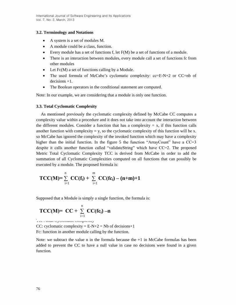
3.2. Terminology and Notations

A system is a set of modules M.

A module could be a class, function.

Every module has a set of functions f, let F(M) be a set of functions of a module.

There is an interaction between modules, every module call a set of functions fc from

other modules

Let Fc(M) a set of functions calling by a Module.

The used formula of McCabe’s cyclomatic complexity: cc=E-N+2 or CC=nb of

decisions +1.

The Boolean operators in the conditional statement are computed.

Note: In our example, we are considering that a module is only one function.

3.3. Total Cyclomatic Complexity

As mentioned previously the cyclomatic complexity defined by McCabe CC computes a

complexity value within a procedure and it does not take into account the interaction between

the different modules. Consider a function that has a complexity = x, if this function calls

another function with complexity = y, so the cyclomatic complexity of this function will be x.

so McCabe has ignored the complexity of the invoked function which may have a complexity

higher than the initial function. In the figure 5 the function “ArrayCount” have a CC=3

despite it calls another function called “validateString” which have CC=2. The proposed

Metric Total Cyclomatic Complexity TCC is derived from McCabe in order to add the

summation of all Cyclomatic Complexities computed on all functions that can possibly be

executed by a module. The proposed formula is:

Supposed that a Module is simply a single function, the formula is:

Tcc : total Cyclomatic complexity

CC: cyclomatic complexity = E-N+2 = Nb of decisions+1

Fc: function in another module calling by the function.

Note: we subtract the value n in the formula because the +1 in McCabe formulas has been

added to prevent the CC to have a null value in case no decisions were found in a given

function.

n m

TCC(M)= ∑ CC(fi) + ∑ CC(fci) – (n+m)+1 i=1 i=1

n

TCC(M)= CC + ∑ CC(fci) –n i=1


Vol. 7, No. 2, March, 2013

77

Figure 5. An Example of Interaction between Modules

Void ArrayCount

(Array A[])

{

IntNbSum =0;

IntNbString = 0;

For (i=0 ; i<A.length ;

i++)

{

if

( validateString(a[i])=

=0)

NbSum++;

Else

NbString ++;

}

Instruction ..

}

IntvaliddateString

(string S)

{

If (isNumber(S))

Return 0;

Else

Return 1 ;

}

Void IsNumber (String

S)

{

Boolean b= true;

For

(i=0,i<S.length,i++)

{

If ((ASCI(CharAT(i)) >

value) &

(ASCI(CharAT(i)) <

value))

B=true ;

Else

Break;

}


Vol. 7, No. 2, March, 2013

78

Example:

Based on the figure 5, TCC is calculated from the function ArrayCount . The function

ArrayCount has a CC value of 3 [( 2 decisions for – if )+1]. Now ,we follow the functions call

by Array count :

ArrayCount call one function ValidateString in Module B

ValidateString : has a CC value of 2 [(1decision – if)+1]

For the same way ValidateString call one function IsNumber in Module C

IsNumber: has a CC value of 4 [(3 decisions –for –if -&) +1]

By applying the formula above: The TCC of Function ArrayCount is the sum of all these

computed CC values which is 7.

TCC (ArrayCount) = CC (ArrayCount) + ∑ TCC(fci) - 1

= 3 + [CC (ValidateString) + ∑ TCC(fci) -1 ] -1

= 3 +[ 2 + CC(IsNumber)-1] -1

= 3 +[ 2 +4-1] -1

= 7

Figure 6. Total Cyclomatic Complexity of Function ”ArrayCount”= 7


Vol. 7, No. 2, March, 2013

79

3.4. Evaluation of the Formula

The formula described previously was developed to take into account the complexity of

modules calling when calculating the complexity of a module. But by simply adding the CC

to the other modules, the coupling or the complexity of intra–modules is not evaluated. The

influence of interactions between modules on complexity is clear and had been explained

earlier. Coupling is considered as an important factor that leads to a bad design. Based on the

example in Figure 7, if we have the same code written in a single function as shown in Figure

5, the same value of TCC will be reached. So, a code written in only one module or divided

into many modules would have the same complexity value!?

Note that a module is not only a simple function; it could also be a class, package…

This will drive us to think about adding a variable that takes a value based on the interactions

between modules.

Figure 7. Control Graph for the Function TotalArrayCount

3.5. Coupled Cyclomatic Complexity

The interaction between modules issue has been asked frequently as it has a real impact in

measuring complexity. This will make clear the influence of coupling. For this reason we will

introduce a variable called α coupling value to represent the intra-modular complexity. The

value of α coupling value is related to the level of coupling. There exist five types of

coupling: content Coupling is the worst.

The table below summarize the α coupling value attributed to the coupled level:


Vol. 7, No. 2, March, 2013

80

Table 1. The Coupling Value of α

Coupling Value

α

Coupling type Description

1 Data A module passes data through scalar or array

parameters to the other module

2 Stamp A module passes a record type variable as a

parameter to the other module

3 Control A module passes a flag value that is used to control

the internal logic of the other.

4 Global Two modules refer to the same global data.

5 Content a module refers to the internals of another module

The notion of α Coupling Value is proposed to adding a value of interaction between

modules. It takes into account the inter-modular complexity.

The supposed formula is:

CCC :Coupled Cyclomatic complexity

CC : cyclomatic complexity = E-N+2 = Nb of decisions+1

Fc : function in another module Calling by the function.

α: Coupling value

The Coupled Cyclomatic Complexity CCC(m) computes the CC for all the functions called.

However, at each calculation of the CC it is multiplied by the (α coupled value).

Note: if exist more than coupling between two modules, we take the maximum value.

Example:

Based on the Figure 6, CCC is calculated from the function ArrayCount. The function

ArrayCount has a CC value of 3 [( 2 decisions for – if )+1] or E-n=2.

Now, we follow the functions called by Array count:

ArrayString() call one function ValidateString()

ValidateString() is a function in Module B called by Module A : has a CC value of 2

[(1decision – if)+1]

Since a[i] in function ArrayCount() is passed to the function ValidateString() as a data

value, modules A and B are data coupled: the α Coupled value =1.

However, the value returned from validatString() is used to control the logic of function

ArrayCount(), resulting in control coupling between the two modules: the α Coupled value =3

in the same way IsNumber() is a function in Module C called by Module B :

it has a CC value of 4 [(3 decisions –for –if -&) +1]

the α Coupled value of the two modules B and C = 3


Vol. 7, No. 2, March, 2013

81

By applying the above formula: The CCC of function ArrayCount() is the sum of all these

computed CC values which is 32

CCC (ArrayCount) = CC (ArrayCount) + ∑ αi CC(fci) - 1

= 3 + 3* [ CC(ValidateString) + ∑ α CCC(fci) -1] -1

= 3 + 3* [ 2 + 3*(CC(IsNumber)-1) -1] -1

= 3 + 3*( 2 +[3*(4 -1)] -1) -1

= 3 + 3*( 2 +9 -1) -1

= 32

3.6. Evaluation

Our objective was finding a metric that works on design phase and handle the complexity

issue. The two suggested formula: Total Cyclomatic Complexity and Coupled Cyclomatic

complexity combine the intra-modular and inter-modular complexity which involve the entire

target of measuring complexity. It is based on the cyclomatic complexity that is applicable in

design phase. The recursively in the two proposed formulas is used because we want to

calculate the complexity of all the modules that interact together. The notion of coupling in

the cyclomatic complexity will give a new vision of calculating the complexity due to its

importance in modularization.

We should put an interval to give the output an accurate meaning. The alpha values should

be confirmed.

4. Conclusion and Future Work

We have done the metric first to achieve the quality corresponding to a goal (reduce cost of

maintainability, assure a secure system). The metrics used for evaluating the software have a

big impact on the objective, so a clever decision should be taken about what metric(s) would

be more efficient according to the requirements of the software. Once the goal is specified,

we can found a diversity of existing metrics that can be appropriate. But the large number of

metrics for a specific goal becomes very confusing, because it will give a diversity of values

with different intervals that can be difficult to evaluate. The conjunction of different metric(s)

might be useful. If we can find a metric that encompass all the aspects of our goal, it would be

a good step toward successful software.

In this paper, our goal is measuring the complexity of software in design phase for two

reasons:

The complexity is an important factor that defines the quality of software starting from

reusability, understandability ending with the cost of maintenance. Measuring the complexity

in design phase can achieve many advantages in quality, due to the contribution of this phase

in reducing the cost and effort of redesign and maintainability. So we try to find a suitable

metric to measure the two aspects of complexity in the design phase: inter-modular and intra-

modular complexity. There exist many metrics that measure the complexity of software: The

cyclomatic complexity metric provides a means of quantifying intra-modular software

complexity, and its utility has been suggested in the software development and testing process.

Other metrics also measures the inter-modular complexity. However, because no one existing

metric can realize our goal, we propose a new approach of measuring complexity which is

based on cyclomatic complexity and the concept of interaction between modules that we

suppose it would be more efficient.

The quality is still the final purpose of searching and implementing different metrics. The

effect of the proposed formulas on the quality should be proven in future experiments. For the


Vol. 7, No. 2, March, 2013

82

reason that reducing complexity and coupling is somehow would reduce in turn the number of

defects in software and faraway will reduce the cost of the maintenance procedures and

facilitate the reuse and the understandability of the code. Our future work is to make some

excessive work and tentative by applying the two new mentioned formulas on a diversity of

modules with different types of coupling to give a more accurate interval to TCC and CCC.

We should compare the results of these 2 formulas to some existing metrics (cyclomatic

complexity, Halsted).

References

[1]. R. Banker, “Software Complexity And Maintainability”.

[2]. H. Zuse, “Software Complexity:Measures and Methods”, De Gruyter, Berlin, (1991).

[3]. J. Fitzpatrick, “Software Quality:Definitions and Strategic Issues”, Staffordshire University, (1997) April.

[4]. M. Halstead, “Elements of Software Science”, North Holland, (1977).

[5]. D. Card and W. Agresti, “Measuring Software Design Complexity”, Journal of Systems and Software,

(1988), pp. 185-197.

[6]. T. McCabe, “A Complexity Measure”, IEEE Transactions on Software Engineering, (1976) December.

[7]. T. McCabe, “Structured Testing: A Testing Methodology Using the Cyclomatic Complexity Metric,” NIST

Special Publication, (1996) September, pp. 500-235.

[8]. T. Shimeall, “Cyclomatic Complexity as a Utility for Predicting Software Faults”, (1990) March.

[9]. S. Nystedt, “Software Complexity and Project Performance”, University of Gothenburg, (1999).

[10] K. Geoffrey, “Cyclomatic Complexity Density and Software Maintenance Productivity”, IEEE Transactions

on Software Engineering, vol. 17, no. 12, (1991) December.

[11] I. Chowdhury, “Using Complexity, Coupling, And Cohesion Metrics as Early Indicators of Vulnerabilities”,

Queen’s University Canada, (2009) September.

On the Improvement of Cyclomatic Complexity Metric

Documents

Transcript of On the Improvement of Cyclomatic Complexity Metric