arX

iv:1

101.

0147

v1 [

mat

h.FA

] 3

0 D

ec 2

010

On the Hausdorff dimension of continuous

functions belonging to Hölder and Besov spaces on

fractal d-sets

Abel Carvalho∗and António Caetano†

Abstract

The Hausdorff dimension of the graphs of the functions in Hölder andBesov spaces (in this case with integrability p ≥ 1) on fractal d-sets is studied.Denoting by s ∈ (0, 1] the smoothness parameter, the sharp upper boundmin{d + 1 − s, d/s} is obtained. In particular, when passing from d ≥ s tod < s there is a change of behaviour from d+ 1− s to d/s which implies thateven highly nonsmooth functions defined on cubes in R

n have not so roughgraphs when restricted to, say, rarefied fractals.

MSC 2010: 26A16, 26B35, 28A78, 28A80, 42C40, 46E35.

Keywords: Hausdorff dimension; box counting dimension; fractals; d-sets; con-

tinuous functions; Weierstrass function; Hölder spaces; Besov spaces; wavelets.

Acknowledgements: Research partially supported by Fundação para a Ciência

e a Tecnologia (Portugal) through Centro de I&D em Matemática e Aplicações

(formerly Unidade de Investigação em Matemática e Aplicações) of the University

of Aveiro.

1 Introduction

This paper deals with the relationship between dimensions of sets and of the graphs

of real continuous functions defined on those sets and having some prescribed smooth-

ness. First studies in this direction are reported in [7, Chapter 10, § 7], where

min{d + 1 − s, d/s} is shown to be an upper bound for the Hausdorff dimension

of the graphs of Hölder continuous functions with Hölder exponent s ∈ (0, 1) and

defined on compact subsets of Rn with Hausdorff dimension equal to d.

∗Centro I&D Matemática e Aplicações, Universidade de Aveiro, 3810-193 Aveiro, Portugal,abel.carvalho@ua.pt

†Departamento de Matemática, Universidade de Aveiro, 3810-193 Aveiro, Portugal,acaetano@ua.pt (corresponding author)

1

That the above bound is sharp comes out from [7, Chapter 18, § 7]

A corresponding result involving Besov spaces, on cubes on Rn, with smoothness

parameter s ∈ (0, 1] and integrability parameter p ∈ (0,∞] was established by F.

Roueff [11, Theorem 4.8, p. 77], where it turned out that for p ≥ 1 the sharp upper

bound is n+1− s. On the other hand, if upper box dimension is used instead, then

the complete picture was settled by A. Carvalho [2], with A. Deliu and B. Jawerth

[3] as forerunners (though the latter paper contains a mistake noticed by A. Kamont

and B. Wolnik [8] as well as, independently, by A. Carvalho [2]).

Our aim here is to study the corresponding problem for Besov spaces when the

underlying domains for the functions are allowed to have themselves non-integer

dimensions (as was the case in the mentioned results involving Hölder spaces). More

precisely, we consider d-sets in Rn (with 0 < d ≤ n) for our underlying domains

and determine the sharp upper bound for the Hausdorff dimension of the graphs

of continuous functions defined on such d-sets and belonging to Besov spaces (with

integrability parameter p ≥ 1), with a prescribed smoothness parameter s ∈ (0, 1].

As in the case of Hölder spaces, under the assumption s ≤ d we obtain the behaviour

d+ 1− s, whereas when s > d the correct sharp upper bound is d/s.

One of the qualitative implications of this change of behaviour for small values

of d is the following (we illustrate it in the case of Hölder continuous functions):

Given s ∈ (0, 1], n ∈ N and a positive integer d ∈ (0, n], it is possible to find

an Hölder continuous functions defined on a cube in Rn and with Hölder exponent

s whose restriction to some d-set has graph with roughness (as measured by the

Hausdorff dimension) as close to d + 1 − s as one wishes. In particular, if we start

with an s close to zero, our restriction to a d-set might give us a function with a

graph having dimension close to d + 1. This is also true for d ∈ (0, 1) as long as

d ≥ s, so in such cases the graphs of our functions, even when these are restricted to

d-sets with small d, might gain almost one extra unit of roughness when compared

with the domain. Consequently we might be near the right endpoint of the interval

obtained in Lemma 2.10. However, when d is allowed to become less than s, the

dimension of the corresponding graphs cannot overcome d/s, so letting d tend to

zero will result in graphs with dimensions also approaching zero. In other words, in

such cases we are definitely near the left endpoint of the interval obtained in Lemma

2.10.

So we show that the same type of phenomenon occurs in the setting of Besov

spaces. The proof of the upper bound d+1−s is inspired in the deep proof given by

Roueff in the case of having n-cubes for domains. On the other hand, the proof of

the sharpness owes a lot to the ideas used by Hunt [5], where a combination between

randomness and the potential theoretic method for the estimation of Hausdorff

2

dimensions has been used.

For the sake of completeness and to help having the more complex results in

perspective, we revisit also the simpler setting of Hölder spaces and give shorter

proofs than in the setting of Besov spaces. For the reader only interested in the

result involving Hölder continuous functions, some material can be skipped: Lemma

2.11; everything after Example 2.16 within subsection 2.2; Theorem 3.3 (and its long

proof, of course); everything after the first paragraph in the proof of Corollary 3.4.

This material has specifically to do with the proof involving Besov spaces.

2 Preliminaries

In this section we give the necessary definitions concerning the dimensions, sets and

function spaces to be considered. We also recall some results and establish others

that will be needed for the main proofs in the following section. However, we start

by listing some notation which applies everywhere in this paper:

The number n is always considered in N. The closed ball in Rn with center a and

radius r is denoted by Br(a) and a cartesian product of n intervals of equal length

is said to be an n-cube. The notation | · | stands either for the Euclidean norm in Rn

or for the sum of coordinates of a multi-index in Nn0 and λn denotes the Lebesgue

measure in Rn.

The shorthand diam is used for the diameter of a set and oscIf stands for the

oscillation of the function f on the set I (that is, the difference supI f − infI f),

whereas Γ(f) denotes the graph of the function f . The usual Schwartz space of

functions on Rn is denoted by S(Rn), its dual S ′(Rn) being the usual space of

tempered distributions.

On the relation side, a . b (or b & a) applies to nonnegative quantities a and b

and means that there exists a positive constant c such that a ≤ cb, whereas a ≈ b

means that a . b and b . a both hold. On the other hand, A ⊂ B applies to sets

A and B and is the usual inclusion relation (allowing also for the equality of sets).

We use A →֒ B when continuity of the embedding is also meant, for the topologies

considered in the sets A and B.

2.1 Dimensions, sets and functions

We start with the dimensions, after recalling some notions related with measures.

These definitions and results are taken from [4], to which we refer for details.

Definition 2.1. (a) A measure on Rn is a function µ : P(Rn) → [0,∞], defined

over all subsets of Rn, which satisfies the following conditions: (i) µ(∅) = 0; (ii)

3

µ(U1) ≤ µ(U2) if U1 ⊂ U2; (iii) µ(∪k∈NUk) ≤∑

k∈N µ(Uk), with equality in the case

when {Uk : k ∈ N} is a collection of pairwise disjoint Borel sets.

(b) A mass distribution on Rn is a measure µ on Rn such that 0 < µ(Rn) <∞.

(c) The support of a measure µ is the smallest closed set A such that µ(Rn\A) = 0.

Definition 2.2. Let d ≥ 0, δ > 0 and ∅ 6= E ⊂ Rn.

(a) We define Hdδ(E) := inf{

∑

k∈N diam (Uk)d : diam (Uk) ≤ δ and E ⊂ ∪k∈NUk}.

(b) The quantity Hdδ(E) increases when δ decreases. Hence the following defi-

nition, of the so-called d-dimensional Hausdorff measure, makes sense: Hd(E) :=

limδ→0+ Hdδ(E). And it is, indeed, a measure according to the preceding definition.

(c) There exists a critical value dE ≥ 0 such that Hd(E) = ∞ for d < dE and

Hd(E) = 0 for d > dE. We define the Hausdorff dimension of E as dimH E := dE.

Remark 2.3. In order to get to the definiton of Hausdorff dimension of the set E

we can restrict consideration to sets Uk which are n-cubes, with sides parallel to the

axes, of side length 2−j, with j ∈ N, and centered at points of the type 2−jm, with

m ∈ Zn. This can lead to different values for measures, but will produce the same

Hausdorff dimension as in the definition above. We shall take advantage of this later

on.

We collect in the following remark some properties concerning Hausdorff dimen-

sion that we shall also need:

Remark 2.4. (a) dimH Rn = n. More generally, the same is true for the dimension

of any open subset of Rn.

(b) If E ⊂ F , then dimH E ≤ dimH F .

(c) The (Hausdorff) dimension does not increase under a Lipschitzian transfor-

mation of sets.

(d) Consider a closed subset E of Rnand a mass distribution µ supported on E.

Let t > 0 be such that´

Rn

´

Rn1

|x−y|t dµ(x) dµ(y) <∞. Then dimH E ≥ t.

Definition 2.5. Let E be a non-empty bounded subset of Rn. The upper box count-

ing dimension of E is the number

dimBE := lim supj→∞

log2Nj(E)

j,

where Nj(E) stands for the number of n-cubes, with sides parallel to the axes, of side

length 2−j and centered at points of the type 2−jm, with m ∈ Zn, which intersect

E.

Again, we collect in a remark some properties which will be of use later on:

4

Remark 2.6. (a) Let E be a non-empty bounded subset of Rn. Then dimH E ≤

dimBE.

(b) Let ∅ 6= E ⊂ Rn, ∅ 6= F ⊂ Rm, with E bounded. Then dimH(E × F ) ≤

dimBE + dimH F .

Next we define the sets which we want to consider:

Definition 2.7. Let 0 < d ≤ n. A d-set in Rn is a (compact) subset K of Rn which

is the support of a mass distribution µ on Rn satisfying the following condition:

∃c1, c2 > 0 : ∀r ∈ (0, 1], ∀x ∈ K, c1rd ≤ µ(Br(x)) ≤ c2r

d.

Remark 2.8. Here we are not following [4], but rather [6], just with the difference

that our d-sets are necessarily compact, because we are assuming that our associated

measure µ is actually a mass distribution. Otherwise we can follow [6] and conclude

that we can take for µ the restriction to K of the d-dimensional Hausdorff measure

and that a d-set has always Hausdorff dimension equal to d.

Remark 2.9. Any d-set K in Rn, with d ∈ (0, n], intersects ≈ rd cubes of any given

regular tessellation of Rn by cubes of sides parallel to the axes and side length r−1,

for any given r ≥ r0 > 0, r0 fixed, with equivalence constants independent of r. For

a proof, adapt to our setting the arguments in [10, Lemma 2.1.12].

As we shall be interested, later on, to study dimensions of graphs of functions, we

consider here a couple of results involving these special sets. We start with a result

which gives already some restrictions for the possible values that the Hausdorff

dimension of such sets can have.

Lemma 2.10. If f is a real function defined on a d-set K, then dimH Γ(f) ∈

[d, d+ 1].

Proof. (i) We prove first that dimH Γ(f) ≥ d. Writing the elements of Γ(f) in the

form (x, t), with x ∈ K ⊂ Rn and t = f(x) ∈ R, it is clear that K = PΓ(f),

where P : Rn+1 → Rn is the projection defined by P (x, t) := x. As is easily seen,

P is a Lipschitzian transformation of sets, therefore, by Remarks 2.8 and 2.4(c),

d = dimH K ≤ dimH Γ(f).

(d) In order to show that, on the other hand, dimH Γ(f) ≤ d+1, just notice that

Remarks 2.4(a),(b), 2.6(b), 2.9 and Definition 2.5 allow us to write that

dimH Γ(f) ≤ dimH K × R ≤ dimBK + 1 = d+ 1.

Next we state and prove a seed for the so-called aggregation method considered

in [11, p. 24, discussion after Remark 2.2]:

5

Lemma 2.11. Let k, l ∈ N0, with k < l, and h0, h1 be two bounded real functions

defined on a bounded subset K of Rn. Let Qj, with j = k, l, be finite coverings of

K by n-cubes Qj with sides parallel to the axes, of side length 2−j and centered at

points of the type 2−jm, with m ∈ Zn. Assume that a covering of Γ(h0) by (n+ 1)-

cubes of side length at least 2−k is given, and such that over each Qk each point

between the levels mQk:= infQk∩K h0 and MQk

:= supQk∩K h0 belongs to one of

those (n + 1)-cubes. Then the number of (n + 1)-cubes of side length 2−l that one

needs to add to the given covering of Γ(h0), in order to get a covering of Γ(h0 + h1)

by (n + 1)-cubes of side length at least 2−l, and such that over each Ql each point

between the levels mQl:= infQl∩K h0 + h1 and MQl

:= supQl∩K h0 + h1 belongs to

one of those (n+ 1)-cubes, is bounded above by∑

Ql∈Ql

(2l+1 supy∈Ql

|h1(y)|+ 2).

Proof. Clearly what one needs is to cover the portion of Γ(h0+h1) over each Ql and

then put all together. Notice that, given one such Ql, what one really needs to cover

is the portion of Γ(h0+h1) over Qk∩Ql, for the Qkcontaining Ql. By hypothesis, all

the points of Rn+1over Qk∩Ql between the levels mQkand MQk

are already covered,

so one only needs to ascertain which points of Γ(h0+h1) over Qk ∩Ql (= Ql) do not

fall within those levels. Since

mQk− sup

y∈Ql

(−h1(y)) = mQk+ inf

y∈Ql

h1(y) ≤ h0(x) + h1(x) ≤MQk+ sup

y∈Ql

h1(y)

for all x ∈ Ql∩K, then it is enough to add, over Ql, to the previous cover, a number

of (n+1)-cubes of side length 2−l in a quantity not exceeding 2 (2l supy∈Ql|h1(y)|+

1).

We shall also need a couple of technical lemmas which we state and prove next:

Lemma 2.12. Let β > α > 0 be two fixed numbers and ζ : (0, β) → R+ be a fixed

integrable function. Thenˆ α

0

ζ(r)f(r) dr ≈

ˆ β

0

ζ(r)f(r) dr

for all non-increasing functions f : (0, β) → R+.

Proof.´ β

αζ(r)f(r) dr ≤

´ β

αζ(r)f(α) dr = c

´ α

0ζ(r)f(α) dr ≤

´ α

0ζ(r)f(r) dr.

Lemma 2.13. Consider 0 < d ≤ n and K a d-set. Assume that µK is a mass

distribution supported on K according to Definition 2.7. Thenˆ

Rn

f(|x− y|) dµK(x) ≈

ˆ diamK

0

rd−1f(r) dr

for all y ∈ K and all non-increasing and continuous functions f : R+ → R+.

6

Proof. Let R ∈ (0,∞) be such that K ⊂ BR(y), with R chosen independently of

y (this is possible, due to the boundedness of K). By the definition of d-set, there

exists c1, c2 > 0 (also independent of y) such that

c1rd ≤ µK(Br(y)) ≤ c2r

d, for all r ∈ (0, R].

For any λ ∈ (0, R), consider the annulus

C(λ) := {x ∈ Rn : R− λ < |x− y| ≤ R}

and, for any N ∈ N, the partition {Cl : l = 1, . . . , N} of this annulus, where

Cl := {x ∈ Rn : R−

lλ

N< |x− y| ≤ R−

(l − 1)λ

N}, for l = 1, . . . , N.

We have the following estimations:

ˆ

C(λ)

f(|x− y|) dµK(x) ≤N∑

l=1

µK(Cl)f(R−lλ

N)

= εN +N∑

l=1

µK(Cl)f(R−(l − 1)λ

N)

≤ εN +

N∑

l=1

(c2rdl−1 − c2r

dl )f(rl−1)

≤ εN +

ˆ R

(c1/c2)1/d(R−λ)

d(c2rd)

drf(r) dr

= εN + c2d

ˆ R

(c1/c2)1/d(R−λ)

rd−1f(r) dr

where rl := c−1/d2 µK(BR−lλ/N (y))

1/d, so rl ≤ R − lλN

, l = 0, . . . , N . Furthermore, εN

equals

N∑

l=1

µK(Cl)(f(R−lλ

N)− f(R−

(l − 1)λ

N))

≤ µK(C(λ)) max

l=1,...,N|f(R−

lλ

N)− f(R−

(l − 1)λ

N)|,

from which follows (using the uniform continuity of f in [R−λ,R]) that limN→∞ εN =

0. In this way we obtainˆ

C(λ)

f(|x− y|) dµK(x) ≤ c2d

ˆ R

(c1/c2)1/d(R−λ)

rd−1f(r) dr. (1)

And, by similar calculations,ˆ

C(λ)

f(|x− y|) dµK(x) ≥ c1d

ˆ R

(c2/c1)1/d(R−λ)

rd−1f(r) dr, (2)

7

as long as we only consider values of λ ∈ (0, R) close enough to R, so that (c2/c1)1/d(R−

λ) < R. Letting now λ tend to R in (1) and (2), we get (using also the fact that

µK({0}) = 0)

c1d

ˆ R

0

rd−1f(r) dr ≤

ˆ

Rn

f(|x− y|) dµK(x) ≤ c2d

ˆ R

0

rd−1f(r) dr.

The required result now follows by applying Lemma 2.12.

Example 2.14. As an interesting application of the preceding result, which will be

useful to us later on, we haveˆ

K

1

|x− y|udµK(x) ≈

ˆ diamK

0

rd−u−1 dr,

with equivalence constants independent of y ∈ K and u ≥ 0.

2.2 Function spaces

Definition 2.15. For s ∈ (0, 1] and ∅ 6= K ⊂ Rn, define Cs(K) := {f : K → R :

∃c > 0 : ∀x, y ∈ K, |f(x)− f(y)| ≤ c |x− y|s}. In particular, all functions in Cs(K)

are continuous (of course, considering inK the metric inherited from the sorrounding

Rn). We shall call Cs(K) the set of the (real) Hölder continuous functions (over K)

of exponent s. On the other hand, given r ∈ N, we denote by Cr(Rn) the set of

all complex-valued functions defined on Rn such that the function itself and all its

derivatives up to (and including) the order r are bounded and uniformly continuous.

The following is a non-trivial example of a function in Cs(K). Its proof follows

from an easy adaptation of a corresponding result in [5, p. 796].

Example 2.16. x 7→ Ws,θ(x) :=∑n

i=1

∑∞j=0 ρ

−js cos(ρjxi + θij) is Hölder contin-

uous of exponent s ∈ (0, 1) on any bounded subset of Rn, with Hölder constant

independent of θ.

The following definition (of Daubechies wavelets) includes an existence assertion.

For details, we refer to [15, section 3.1].

Definition 2.17. Let r ∈ N. Define L0 := 1 and L := Lj := 2n − 1 if j ∈ N. There

exist compactly supported real functions ψ0 ∈ Cr(Rn) and ψl ∈ Cr(Rn), l = 1, . . . , L

( with

ˆ

Rn

xαψl(x) dx = 0, α ∈ Nn0 , |α| ≤ r ), (3)

such that {Ψljm : j ∈ N0, 1 ≤ l ≤ Lj , m ∈ Zn} is an orthonormal basis in L2(R

n),

where, by definition,

Ψljm(x) :=

{

ψ0(x−m) if j = 0, l = 1, m ∈ Zn

2j−12

nψl(2j−1x−m) if j ∈ N, 1 ≤ l ≤ L, m ∈ Zn.

8

The Besov spaces in the following definition are the usual ones (up to equivalent

quasi-norms), defined by Fourier-analytical tools (a definition along this line can be

seen in [15, section 1.3], for example). From this point of view the definition which

follows is actually a theorem: for details, see [15, Theorem 3.5 and footnote in p.

156].

Definition 2.18. Let 0 < p, q ≤ ∞, s ∈ R and r be a natural number such that

r > max{s, n(1/p− 1)+ − s}. The Besov space Bspq(R

n) is the set of all sums

f :=∑

j,l,m

λljm2−jn/2Ψl

jm =

∞∑

j=0

Lj∑

l=1

∑

m∈Zn

λljm2−jn/2Ψl

jm (4)

(convergence — actually, unconditional convergence — in S ′(Rn)), for all given

sequences {λljm ∈ C : j ∈ N0, l = 1, . . . , Lj , m ∈ Zn} such that

(

∑

m∈Zn

|λ10m|p

)1/p

+L∑

l=1

∞∑

j=1

2j(s−n/p)q

(

∑

m∈Zn

|λljm|p

)q/p

1/q

(5)

(with the usual modifications if p = ∞ or q = ∞) is finite. It turns out that (5)

defines a quasi-norm in Bspq(R

n) which makes this a complete space.

Remark 2.19. (a) The representation (4) is unique, that is, it is uniquely determined

by the limit f , namely the coefficients are determined by the formulæ

λljm = 2jn/2(f,Ψljm), j ∈ N0, l = 1, . . . , Lj , m ∈ Z

n,

where (·, ·), though standing for the inner product in L2(Rn) when applied to func-

tions in such a space, must in general be understood in the sense of the dual pairing

S(Rn) − S ′(Rn) — see [15, section 3.1] for details. As a consequence, when f is

compactly supported, then, given any j ∈ N0, only finitely many coefficients λljm are

non-zero.

(b) Arguing as in [11, p. 21], we can say that the convergence in (4) is even

uniform in the support of f whenever this support is compact and f is a continuous

function.

Definition 2.20. Consider 0 < d ≤ n and K a d-set with associated mass distri-

bution µ according to Definition 2.7. For 0 < p <∞, we define the Lebesgue space

Lp(K) as the set of all µ-measurable functions f : K → C for which the quasi-norm

given by

‖f‖Lp(K) :=

(ˆ

Rn

|f(x)|p dµ(x)

)1/p

is finite.

9

Definition 2.21. Consider 0 < d ≤ n and K a d-set. Let 0 < p, q < ∞. Assuming

that there exists c > 0 such that

‖ϕ|K‖Lp(K) ≤ c ‖ϕ‖Bspq(R

n), ϕ ∈ S(Rn), (6)

the trace of f ∈ Bspq(R

n) on K is defined by trK f := limj→∞ ϕj|K in Lp(K), where

(ϕj)j ⊂ S(Rn) is any sequence converging to f in Bspq(R

n).

This definition is justified by the completeness of Lp(K) and by the fact that

the restrictions on p, q guarantee that the Schwartz space is dense in the Besov

spaces under consideration. That the definition does not depend on the particular

approaching sequence (ϕj)j is a consequence of (6).

By [14, Theorem 18.6 and Comment 18.7], which holds for d = n too (cf. also [1,

Theorem 3.3.1(i)]), one knows that the assumption (6) holds true when 0 < p <∞,

0 < q ≤ min{1, p} and s = n−dp

. Therefore the trace of functions of Besov spaces on

K is well-defined for that range of parameters.

Since Bspq(R

n) →֒ Bn−dp

p,min1,p(Rn) whenever s > n−d

p, then the trace as defined above

makes sense for functions of the spaces Bspq(R

n), for any 0 < p <∞, 0 < q <∞ and

s > n−dp

. Moreover, since the embedding between the Besov spaces above also hold

when q = ∞, then, though Definition (2.21) can no longer be applied, we define, for

any f ∈ Bsp∞(Rn), with 0 < p < ∞ and s > n−d

p, the trK f by its trace when f is

viewed as an element of Bn−dp

p,min1,p(Rn).

Finally, in the case f ∈ Bs∞q(R

n), with 0 < q ≤ ∞ and s > 0, we define trK f :=

f |K , the pointwise restriction, since, for such range of parameters, the elements of

those Besov spaces are all (represented by) continuous functions (actually, we even

have Bs∞q(R

n) →֒ C(Rn), where the latter space stands for the set of all complex-

valued, bounded and uniformly continuous functions on Rn endowed with the sup

norm).

Remark 2.22. Another way of defining trace on K is by starting to define it by

pointwise restriction when the function is continuous and, at least in the case when

f is locally integrable on Rn, define its trace on K by the pointwise restriction f |K ,

where

f(x) := limr→0

1

λn(Br(x))

ˆ

Br(x)

f(y) dy

for the values of x where the limit exists. It is known (Lebesgue differentiation

theorem) that f = f a.e. (for locally integrable functions f). As is easily seen, the

identity f(x) = f(x) surely holds at any point x where f is continuous.

This is the approach followed by Jonsson and Wallin in [6] (see pp. 14-15), where

they have shown (it is a particular case of [6, Theorem 2 in p. 142]) that, for 0 <

10

d ≤ n, 1 ≤ p, q ≤ ∞ and s > n−dp

, the map f 7→ f |K takes Bspq(R

n) linearly and

boundedly into Lp(K).

Note now that, for this restriction of parameters, both trK f and f |K coincide

with f |K when f ∈ S(Rn). Therefore, at least when we further restrict p and q

to be finite, we get the identity trK f = f |K in Lp(K) for any f ∈ Bspq(R

n), by

a density argument. In the case we still restrict p to be finite but admit q = ∞,

from our definition above we see that trK f is also the trace of f ∈ Bε+n−d

p

p,min1,p(Rn),

for any suitable small ε > 0, where here the parameter “q” is again finite, so also

trK f = f |K in Lp(K). This identity even holds when p = ∞ is admitted, taking

into account that in that situation we are dealing with continuous functions.

Summing up, when 0 < d ≤ n, 1 ≤ p, q ≤ ∞ and s > n−dp

we have trK f = f |K .

Although in [6] both p and q are assumed to be greater than or equal to 1,

we can proceed with our comparative analysis between trK f and f |K even for the

remaining positive values of q. In fact, given 0 < d ≤ n, 1 ≤ p ≤ ∞, 0 < q < 1

and s > n−dp

, and due to the embedding Bspq(R

n) →֒ Bε+n−d

p

p,min1,p(Rn) (which holds for

any suitable small ε > 0), we see, from what was mentioned before, that the trace

of f ∈ Bspq(R

n) can be seen as the trace of f as an element of Bε+n−d

p

p,min1,p(Rn); since in

the latter space the “q” parameter is in the range [1,∞] (actually, it is 1), then we

already know that trK f = f |K here too.

As a consequence we have also the following remark, which will be useful later

on:

Remark 2.23. Consider 0 < d ≤ n and K a d-set. If f is a continuous function

belonging to Bspq(R

n), with 1 ≤ p ≤ ∞, 0 < q ≤ ∞ and s > n−dp

, then trK f = f |K .

Definition 2.24. Consider 0 < d ≤ n and K a d-set. Let 0 < p, q ≤ ∞ and s > 0.

We define the Besov space Bspq(K) as the set of traces of the elements of B

s+n−dp

pq (Rn)

endowed with the quasi-norm defined by

‖f‖Bspq(K) := inf ‖g‖

Bs+n−d

ppq (Rn)

where the infimum runs over all g ∈ Bs+n−d

ppq (Rn) such that trK g = f .

For a motivation for such definition, see [13, sections 20.2 and 20.3]. From the

considerations above it follows that the trace maps Bs+n−d

ppq (Rn) linearly and bound-

edly both into Lp(K) and Bspq(K), where the parameters are as in the preceding

definition.

Proposition 2.25. Consider 0 < d ≤ n and K a d-set. Let 0 < p2 < p1 ≤ ∞,

0 < q ≤ ∞ and s > 0. Then

Bsp1q(K) →֒ B

sp2q(K).

11

A sketch of a proof for this result, at least for d = n, can be seen in [13, Step

2 in p. 165]. The argument is not clear to us when 0 < d < n, but a proof in this

situation can be seen in [9, Proposition 2.18], where quarkonial decompositions were

used. In both cases, a proof with atomic decompositions can also be used instead.

From Remark 2.23 it follows that the trace on a d-set K, with 0 < d ≤ n, of a

continuous function belonging to Bs+n−d

ppq (Rn), with 1 ≤ p ≤ ∞, 0 < q ≤ ∞ and

s > 0, is still a continuous function (on K). In the sequel we shall need a partial

converse for this result, the proof of which is sketched below:

Proposition 2.26. Consider 0 < d ≤ n and K a d-set. Let 1 ≤ p, q ≤ ∞ and

0 < s < 1. Any continuous function in Bspq(K) can be obtained as the trace (or

pointwise restriction) of a continuous function in Bs+n−d

ppq (Rn).

Proof. (i) We start with the case 0 < d < n.

We shall need to consider a Whitney decomposition of Kc by a family of closed

n-cubes Qi and an associated partition of unity by functions φi. We use here the

notations and conventions of [6, pp. 23-24 and 155-157], except that our K here is

in the place of F over there. In particular, xi, si and li shall, respectively, stand for

the center of Qi, its side length and its diameter. Moreover, given f ∈ Bspq(K), the

function Ef is defined by

Ef(x) :=∑

i∈Iφi(x)

1

µK(B6li(xi))

ˆ

|t−xi|≤6li

f(t) dµK(t), x ∈ Kc,

where I is the set of indices i such that si ≤ 1 and µK is the mass distribution

supported on K according to Definition 2.7. Notice that Ef is defined a.e. in Rn,

because the asumption d < n guarantees that K has Lebesgue measure 0.

According to [6, Theorem 3 in p. 155], Ef ∈ Bs+n−d

ppq (Rn), Ef is C∞ in Kc (so, in

particular, it is continuous on Kc) and trKEf = (Ef)|K = f . Since Ef = Ef a.e.,

Ef is a representative of an element of Bs+n−d

ppq (Rn) whose pointwise restriction to K

coincides with f . Since the identity Ef(x) = Ef(x) holds for any x ∈ Kc, where we

already know this function is continuous, it remains to show that Ef is continuous

on K, i.e., that

∀t0 ∈ K, ∀ε > 0, ∃δ > 0 : ∀x ∈ Rn, x ∈ Bδ(t0) ⇒ |Ef(x)− f(t0)| < ε.

The implication being trivially true when x is also in K, we can assume that x ∈

Bδ(t0)∩Kc, in which case we have to arrive to the conclusion that |Ef(x)−f(t0)| < ε.

Pick one Qk containing x and consider tk ∈ K and yk ∈ Qk such that |yk − tk| =

dist{Qk, K}. Notice that |tk − t0| ≤ 3δ and that

|Ef(x)− f(t0)| ≤ |Ef(x)− f(tk)|+ |f(tk)− f(t0)|,

12

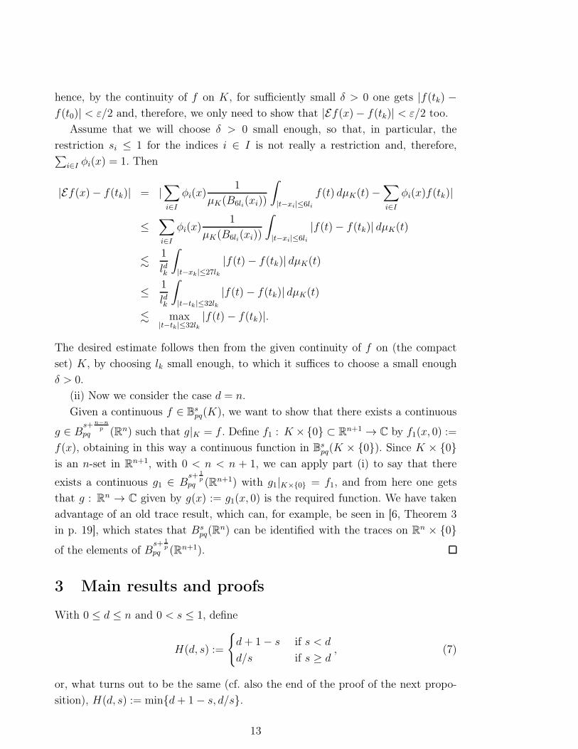
hence, by the continuity of f on K, for sufficiently small δ > 0 one gets |f(tk) −

f(t0)| < ε/2 and, therefore, we only need to show that |Ef(x)− f(tk)| < ε/2 too.

Assume that we will choose δ > 0 small enough, so that, in particular, the

restriction si ≤ 1 for the indices i ∈ I is not really a restriction and, therefore,∑

i∈I φi(x) = 1. Then

|Ef(x)− f(tk)| = |∑

i∈Iφi(x)

1

µK(B6li(xi))

ˆ

|t−xi|≤6li

f(t) dµK(t)−∑

i∈Iφi(x)f(tk)|

≤∑

i∈Iφi(x)

1

µK(B6li(xi))

ˆ

|t−xi|≤6li

|f(t)− f(tk)| dµK(t)

.1

ldk

ˆ

|t−xk|≤27lk

|f(t)− f(tk)| dµK(t)

≤1

ldk

ˆ

|t−tk |≤32lk

|f(t)− f(tk)| dµK(t)

. max|t−tk|≤32lk

|f(t)− f(tk)|.

The desired estimate follows then from the given continuity of f on (the compact

set) K, by choosing lk small enough, to which it suffices to choose a small enough

δ > 0.

(ii) Now we consider the case d = n.

Given a continuous f ∈ Bspq(K), we want to show that there exists a continuous

g ∈ Bs+n−n

ppq (Rn) such that g|K = f . Define f1 : K ×{0} ⊂ Rn+1 → C by f1(x, 0) :=

f(x), obtaining in this way a continuous function in Bspq(K × {0}). Since K × {0}

is an n-set in Rn+1, with 0 < n < n + 1, we can apply part (i) to say that there

exists a continuous g1 ∈ Bs+ 1

ppq (Rn+1) with g1|K×{0} = f1, and from here one gets

that g : Rn → C given by g(x) := g1(x, 0) is the required function. We have taken

advantage of an old trace result, which can, for example, be seen in [6, Theorem 3

in p. 19], which states that Bspq(R

n) can be identified with the traces on Rn × {0}

of the elements of Bs+ 1

ppq (Rn+1).

3 Main results and proofs

With 0 ≤ d ≤ n and 0 < s ≤ 1, define

H(d, s) :=

{

d+ 1− s if s < d

d/s if s ≥ d, (7)

or, what turns out to be the same (cf. also the end of the proof of the next propo-

sition), H(d, s) := min{d+ 1− s, d/s}.

13

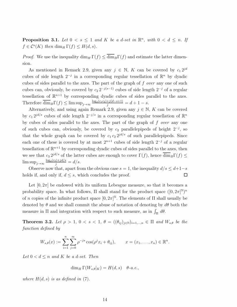
Proposition 3.1. Let 0 < s ≤ 1 and K be a d-set in Rn, with 0 < d ≤ n. If

f ∈ Cs(K) then dimH Γ(f) ≤ H(d, s).

Proof. We use the inequality dimH Γ(f) ≤ dimBΓ(f) and estimate the latter dimen-

sion.

As mentioned in Remark 2.9, given any j ∈ N, K can be covered by c1 2jd

cubes of side length 2−j in a corresponding regular tessellation of Rn by dyadic

cubes of sides parallel to the axes. The part of the graph of f over any one of such

cubes can, obviously, be covered by c2 2−j(s−1) cubes of side length 2−j of a regular

tessellation of Rn+1 by corresponding dyadic cubes of sides parallel to the axes.

Therefore dimBΓ(f) ≤ lim supj→∞log2(c1c2)+j(d−s+1)

j= d+ 1− s.

Alternatively, and using again Remark 2.9, given any j ∈ N, K can be covered

by c1 2jd/s cubes of side length 2−j/s in a corresponding regular tessellation of Rn

by cubes of sides parallel to the axes. The part of the graph of f over any one

of such cubes can, obviously, be covered by c2 parallelepipeds of height 2−j, so

that the whole graph can be covered by c1 c2 2jd/s of such parallelepipeds. Since

each one of these is covered by at most 2n+1 cubes of side length 2−j of a regular

tessellation of Rn+1 by corresponding dyadic cubes of sides parallel to the axes, then

we see that c3 2jd/s of the latter cubes are enough to cover Γ(f), hence dimBΓ(f) ≤

lim supj→∞log2(c3)+jd/s

j= d/s.

Observe now that, apart from the obvious case s = 1, the inequality d/s ≤ d+1−s

holds if, and only if, d ≤ s, which concludes the proof.

Let [0, 2π] be endowed with its uniform Lebesgue measure, so that it becomes a

probability space. In what follows, Π shall stand for the product space ([0, 2π]N)n

of n copies of the infinite product space [0, 2π]N. The elements of Π shall usually be

denoted by θ and we shall commit the abuse of notation of denoting by dθ both the

measure in Π and integration with respect to such measure, as in´

Πdθ.

Theorem 3.2. Let ρ > 1, 0 < s < 1, θ = ((θij)j∈N)i=1,...,n ∈ Π and Ws,θ be the

function defined by

Ws,θ(x) :=

n∑

i=1

∞∑

j=0

ρ−js cos(ρjxi + θij), x = (x1, . . . , xn) ∈ Rn.

Let 0 < d ≤ n and K be a d-set. Then

dimH Γ(Ws,θ|K) = H(d, s) θ-a.e.,

where H(d, s) is as defined in (7).

14

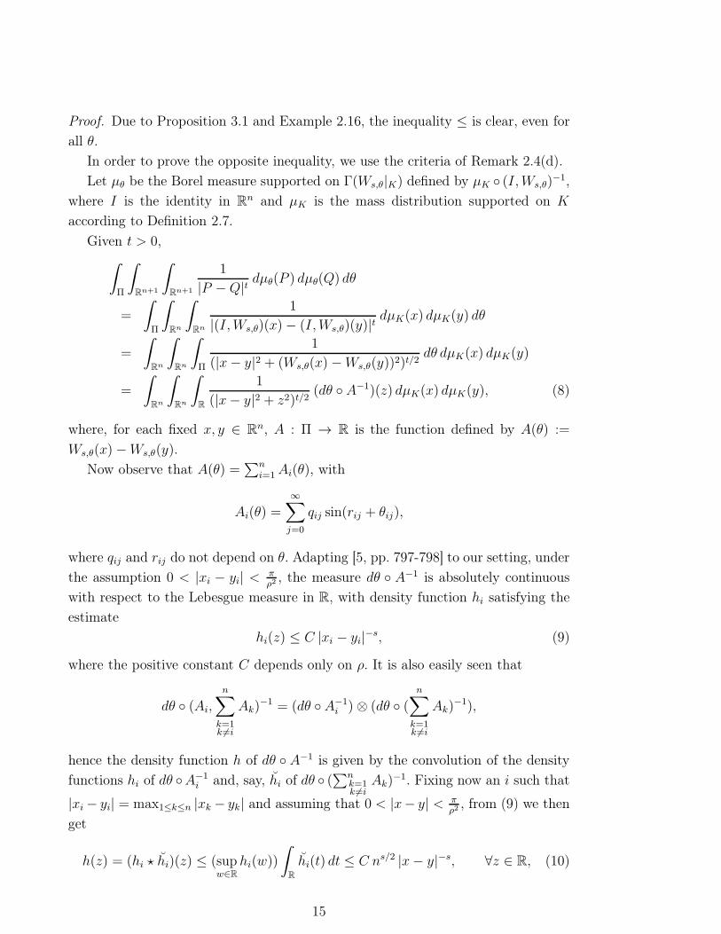
Proof. Due to Proposition 3.1 and Example 2.16, the inequality ≤ is clear, even for

all θ.

In order to prove the opposite inequality, we use the criteria of Remark 2.4(d).

Let µθ be the Borel measure supported on Γ(Ws,θ|K) defined by µK ◦ (I,Ws,θ)−1,

where I is the identity in Rn and µK is the mass distribution supported on K

according to Definition 2.7.

Given t > 0,

ˆ

Π

ˆ

Rn+1

ˆ

Rn+1

1

|P −Q|tdµθ(P ) dµθ(Q) dθ

=

ˆ

Π

ˆ

Rn

ˆ

Rn

1

|(I,Ws,θ)(x)− (I,Ws,θ)(y)|tdµK(x) dµK(y) dθ

=

ˆ

Rn

ˆ

Rn

ˆ

Π

1

(|x− y|2 + (Ws,θ(x)−Ws,θ(y))2)t/2dθ dµK(x) dµK(y)

=

ˆ

Rn

ˆ

Rn

ˆ

R

1

(|x− y|2 + z2)t/2(dθ ◦ A−1)(z) dµK(x) dµK(y), (8)

where, for each fixed x, y ∈ Rn, A : Π → R is the function defined by A(θ) :=

Ws,θ(x)−Ws,θ(y).

Now observe that A(θ) =∑n

i=1Ai(θ), with

Ai(θ) =

∞∑

j=0

qij sin(rij + θij),

where qij and rij do not depend on θ. Adapting [5, pp. 797-798] to our setting, under

the assumption 0 < |xi − yi| <πρ2

, the measure dθ ◦ A−1 is absolutely continuous

with respect to the Lebesgue measure in R, with density function hi satisfying the

estimate

hi(z) ≤ C |xi − yi|−s, (9)

where the positive constant C depends only on ρ. It is also easily seen that

dθ ◦ (Ai,

n∑

k=1k 6=i

Ak)−1 = (dθ ◦ A−1

i )⊗ (dθ ◦ (n∑

k=1k 6=i

Ak)−1),

hence the density function h of dθ ◦ A−1 is given by the convolution of the density

functions hi of dθ ◦A−1i and, say, h̆i of dθ ◦ (

∑nk=1k 6=i

Ak)−1. Fixing now an i such that

|xi − yi| = max1≤k≤n |xk − yk| and assuming that 0 < |x− y| < πρ2

, from (9) we then

get

h(z) = (hi ⋆ h̆i)(z) ≤ (supw∈R

hi(w))

ˆ

R

h̆i(t) dt ≤ C ns/2 |x− y|−s, ∀z ∈ R, (10)

15

where C is the same constant as in (9).

Returning to (8), we can now write, taking into account that the hypotheses

guarantee that (µK ⊗ µK)({x = y}) = 0,ˆ

Π

ˆ

Rn+1

ˆ

Rn+1

1

|P −Q|tdµθ(P ) dµθ(Q) dθ (11)

=

ˆ

Rn×Rn

|x−y|≥ πρ2

ˆ

R

h(z)

(|x− y|2 + z2)t/2dz d(µK ⊗ µK)(x, y)

+

ˆ

Rn×Rn

0<|x−y|< πρ2

ˆ

R

h(z)

(|x− y|2 + z2)t/2dz d(µK ⊗ µK)(x, y),

where the first term on the right-hand side is clearly finite, while, due to (10), the

second term can be estimated from above by

C ns/2

ˆ

Rn×Rn

0<|x−y|< πρ2

ˆ

R

|x− y|−s

(|x− y|2 + z2)t/2dz d(µK ⊗ µK)(x, y)

=C ns/2

ˆ

Rn×Rn

0<|x−y|< πρ2

|x− y|−s+1−t

ˆ

R

1

(1 + w2)t/2dw d(µK ⊗ µK)(x, y). (12)

We now need to split the proof in two cases, in order to proceed.

Case d > s:

Consider

tm := d+ 1− s−1

m,

for sufficiently large m ∈ N so that d− s > 2m

. Then, using tm in the place ot t, the

inner integral in (12) can be estimated from above byˆ

|w|≤1

dw +

ˆ

|w|>1

1

|w|tmdw ≤ 2 +

4

d− s,

hence (12) can be estimated from above by

c1

ˆ

Rn×Rn

0<|x−y|< πρ2

|x− y|−s+1−tm d(µK ⊗ µK)(x, y)

≤ c1

ˆ

Rn

ˆ

Rn

|x− y|−d+1/m dµK(x) dµK(y)

≤ c2

ˆ

K

ˆ diamK

0

r1/m−1 dr dµK(y) < ∞,

where we have used Example 2.14. Therefore, we have proved the finiteness of (11)

when using t = tm = d + 1 − s − 1m

for any sufficiently large natural m, and have

shown in particular, for any such number tm, thatˆ

Rn+1

ˆ

Rn+1

1

|P −Q|tmdµθ(P ) dµθ(Q) <∞ θ-a.e..

16

Consequently, by Remark 2.4(d),

dimH(Γ(Ws,θ|K) ≥ tm = d+ 1− s−1

mθ-a.e.

for any m large enough. Since this is a countable number of possibilities, we can also

state that, for almost all θ ∈ Π, dimH(Γ(Ws,θ|K) ≥ d+ 1− s− 1m

for all previously

considered numbers m, so that the required result follows after letting m tend to

infinity.

Case d ≤ s:

Here we shall take advantage of the fact that the support of dθ◦A−1 is contained

in [−c |x − y|s, c |x − y|s], for some positive constant c (independent of x and y).

That this is the case follows from Example 2.16.

We return then to the decomposition given above for (11) and observe that we

can replace the integral over R in the second term in that decomposition by a

corresponding integral over [−c |x − y|s, c |x − y|s], so that instead of (12) we can

write, up to a constant factor,

ˆ

Rn×Rn

0<|x−y|< πρ2

|x− y|−s+1−t

ˆ c |x−y|s−1

0

1

(1 + w2)t/2dw d(µK ⊗ µK)(x, y), (13)

where, moreover, c |x−y|s−1 can, without loss of generality, be assumed to be greater

than 1.

Consider now

tm :=d

s−

1

m,

for sufficiently large m ∈ N so that tm > 0. Then, using tm in the place ot t, the

inner integral in (13) can be estimated from above by

ˆ 1

0

1

(1 + w2)tm/2dw +

ˆ c |x−y|s−1

1

1

(1 + w2)tm/2dw <

c1−tm

1− tm|x− y|(1−tm)(s−1),

hence (13) can be estimated from above by

c31− tm

ˆ

Rn×Rn

0<|x−y|< πρ2

|x− y|−s+1−tm+(1−tm)(s−1) d(µK ⊗ µK)(x, y)

≤c3

1− tm

ˆ

Rn

ˆ

Rn

|x− y|−d+s/m dµK(x) dµK(y)

≤c4

1− tm

ˆ

K

ˆ diamK

0

rs/m−1 dr dµK(y) < ∞,

where we have used Example 2.14. The rest of the proof follows as in the previous

case, the difference being that now tm = ds− 1

m, therefore tends to d

swhen m goes

to infinity.

17

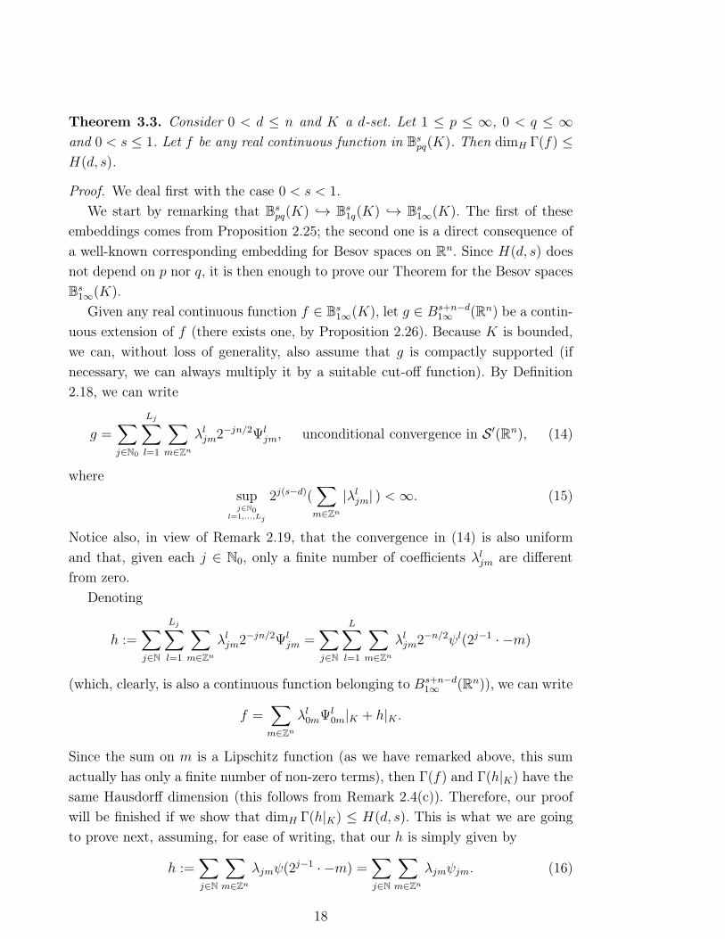
Theorem 3.3. Consider 0 < d ≤ n and K a d-set. Let 1 ≤ p ≤ ∞, 0 < q ≤ ∞

and 0 < s ≤ 1. Let f be any real continuous function in Bspq(K). Then dimH Γ(f) ≤

H(d, s).

Proof. We deal first with the case 0 < s < 1.

We start by remarking that Bspq(K) →֒ Bs

1q(K) →֒ Bs1∞(K). The first of these

embeddings comes from Proposition 2.25; the second one is a direct consequence of

a well-known corresponding embedding for Besov spaces on Rn. Since H(d, s) does

not depend on p nor q, it is then enough to prove our Theorem for the Besov spaces

Bs1∞(K).

Given any real continuous function f ∈ Bs1∞(K), let g ∈ Bs+n−d

1∞ (Rn) be a contin-

uous extension of f (there exists one, by Proposition 2.26). Because K is bounded,

we can, without loss of generality, also assume that g is compactly supported (if

necessary, we can always multiply it by a suitable cut-off function). By Definition

2.18, we can write

g =∑

j∈N0

Lj∑

l=1

∑

m∈Zn

λljm2−jn/2Ψl

jm, unconditional convergence in S ′(Rn), (14)

where

supj∈N0

l=1,...,Lj

2j(s−d)(∑

m∈Zn

|λljm| ) <∞. (15)

Notice also, in view of Remark 2.19, that the convergence in (14) is also uniform

and that, given each j ∈ N0, only a finite number of coefficients λljm are different

from zero.

Denoting

h :=∑

j∈N

Lj∑

l=1

∑

m∈Zn

λljm2−jn/2Ψl

jm =∑

j∈N

L∑

l=1

∑

m∈Zn

λljm2−n/2ψl(2j−1 · −m)

(which, clearly, is also a continuous function belonging to Bs+n−d1∞ (Rn)), we can write

f =∑

m∈Zn

λl0mΨl0m|K + h|K .

Since the sum on m is a Lipschitz function (as we have remarked above, this sum

actually has only a finite number of non-zero terms), then Γ(f) and Γ(h|K) have the

same Hausdorff dimension (this follows from Remark 2.4(c)). Therefore, our proof

will be finished if we show that dimH Γ(h|K) ≤ H(d, s). This is what we are going

to prove next, assuming, for ease of writing, that our h is simply given by

h :=∑

j∈N

∑

m∈Zn

λjmψ(2j−1 · −m) =

∑

j∈N

∑

m∈Zn

λjmψjm. (16)

18

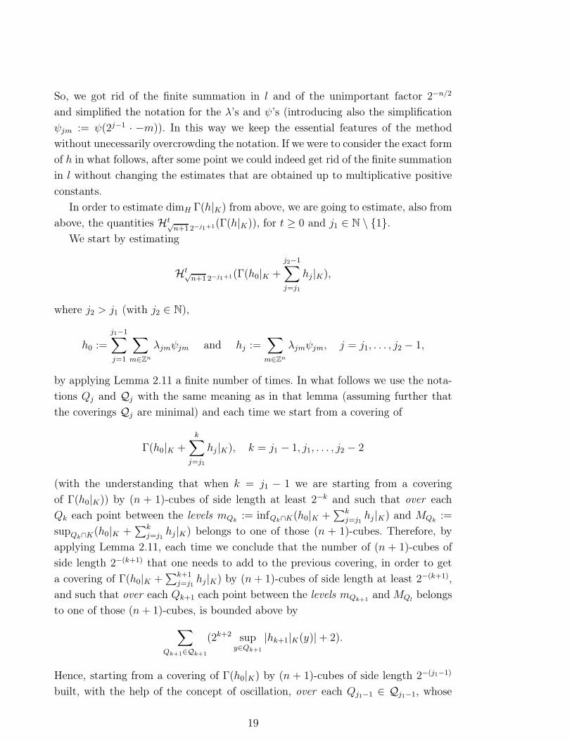
So, we got rid of the finite summation in l and of the unimportant factor 2−n/2

and simplified the notation for the λ’s and ψ’s (introducing also the simplification

ψjm := ψ(2j−1 · −m)). In this way we keep the essential features of the method

without unecessarily overcrowding the notation. If we were to consider the exact form

of h in what follows, after some point we could indeed get rid of the finite summation

in l without changing the estimates that are obtained up to multiplicative positive

constants.

In order to estimate dimH Γ(h|K) from above, we are going to estimate, also from

above, the quantities Ht√n+12−j1+1(Γ(h|K)), for t ≥ 0 and j1 ∈ N \ {1}.

We start by estimating

Ht√n+12−j1+1(Γ(h0|K +

j2−1∑

j=j1

hj |K),

where j2 > j1 (with j2 ∈ N),

h0 :=

j1−1∑

j=1

∑

m∈Zn

λjmψjm and hj :=∑

m∈Zn

λjmψjm, j = j1, . . . , j2 − 1,

by applying Lemma 2.11 a finite number of times. In what follows we use the nota-

tions Qj and Qj with the same meaning as in that lemma (assuming further that

the coverings Qj are minimal) and each time we start from a covering of

Γ(h0|K +k∑

j=j1

hj |K), k = j1 − 1, j1, . . . , j2 − 2

(with the understanding that when k = j1 − 1 we are starting from a covering

of Γ(h0|K)) by (n + 1)-cubes of side length at least 2−k and such that over each

Qk each point between the levels mQk:= infQk∩K(h0|K +

∑kj=j1

hj |K) and MQk:=

supQk∩K(h0|K +∑k

j=j1hj|K) belongs to one of those (n + 1)-cubes. Therefore, by

applying Lemma 2.11, each time we conclude that the number of (n + 1)-cubes of

side length 2−(k+1) that one needs to add to the previous covering, in order to get

a covering of Γ(h0|K +∑k+1

j=j1hj |K) by (n + 1)-cubes of side length at least 2−(k+1),

and such that over each Qk+1 each point between the levels mQk+1and MQl

belongs

to one of those (n+ 1)-cubes, is bounded above by

∑

Qk+1∈Qk+1

(2k+2 supy∈Qk+1

|hk+1|K(y)|+ 2).

Hence, starting from a covering of Γ(h0|K) by (n + 1)-cubes of side length 2−(j1−1)

built, with the help of the concept of oscillation, over each Qj1−1 ∈ Qj1−1, whose

19

number is bounded above by

∑

Qj1−1∈Qj1−1

(2j1−1oscQj1−1h0|K + 2),

and applying Lemma 2.11 repeatedly (a total number of j2 − j1 times), we get the

following estimates (the constants might depend on t), where we have also used

Remark 2.9 to estimate the number of elements of each Qj :

Ht√n+12−j1+1(Γ(h0|K +

j2−1∑

j=j1

hj |K))

. 2−j1t∑

Qj1−1∈Qj1−1

(2j1−1oscQj1−1h0|K + 2)

+

j2−1∑

j=j1

2−jt∑

Qj∈Qj

(2j+1 supy∈Qj

|hj |K(y)|+ 2)

. 2−j1(t−d) + 2−j1(t−1)∑

Qj1−1∈Qj1−1

oscQj1−1h0|K (17)

+

j2−1∑

j=j1

2−j(t−d) +

j2−1∑

j=j1

2−j(t−1)∑

m∈Zn

|λjm|.

The estimate in the last term is possible because of the controlled overlapping be-

tween the support of each ψjm and the different Qj ’s (i.e., each suppψjm intersects

only a finite number of Qj ’s and this number can be bounded above by a constant

independent of j).

Now, if one wants to estimate Ht√n+12−j1+1(Γ(h|K)) instead, notice that the

Lemma 2.11 can again be used, and we just have to find out what is the contri-

bution, coming from∑∞

j=j2hj |K , that we need to add to the right-hand side of (17).

Actually, this could have been done at the same time we added the contribution of

the term hj1|K , resulting in the extra term

2−j1(t−1)∑

Qj1∈Qj1

supy∈Qj1

|∞∑

j=j2

hj|K(y)|

. 2−j1(t−1)2j1d supy∈Rn

|∞∑

j=j2

hj|K(y)| =: 2−j1(t−1)2j1dCj2 .

However, by the already mentioned uniform convergence of the sum defining h, we

have that Cj2 tends to 0 as j2 goes to infinity. Therefore, by choosing j2 large enough

(in dependence of j1) so that Cj22j1 ≤ 1, the last contribution is just of the type

2−j1(t−d). This is the same as the first term in (17), and both can be absorbed by

20

the third term in that expression. Hence, for such a choice of j2,

Ht√n+12−j1+1(Γ(h|K)). (18)

.

j2−1∑

j=j1

2−j(t−d) + 2−j1(t−1)∑

Qj1−1∈Qj1−1

oscQj1−1h0|K +

j2−1∑

j=j1

2−j(t−1)∑

m∈Zn

|λjm|.

Now we estimate separately each one of the three distinguished terms above (in

all cases ignoring unimportant multiplicative constants):

The first one is dominated by 2−j1(t−d) under the assumption t > d.

The second one is dominated by

2−j1(t−1)∑

Qj1−1∈Qj1−1

j1−1∑

j=1

∑

m

oscQj1−1(λjmψjm|K)

≤ 2−j1(t−1)

j1−1∑

j=1

∑

m

∑

Qj1−1∈Qj1−1

|λjm| |∇ψjm(ξj1)| 2−j1, (19)

where ξj1 is chosen in Qj1−1 in accordance with the mean value theorem (which

we have just used above) and in∑

m the m is restricted to the values for which

suppψjm intersects K. Such a number of m’s can clearly be estimated from above

by 2jd (cf. Remark 2.9 and Definition 2.17). Next we remark that |∇ψjm(ξj1)| . 2j

and that in the inner sum in (19) we only need to consider the Qj1−1’s which intersect

suppψjm. It is not difficult to see that such a number of Qj1−1’s can be estimated

from above by 2(j1−j)d. Putting all this together, and using also the estimate (15)

and the hypothesis 0 < s < 1, the second term on the right-hand side of (18) is

dominated by

2−j1(t−1)

j1−1∑

j=1

2j−j12(j1−j)d∑

m∈Zn

|λjm|

. 2−j1(t−d)j1 max1≤j≤j1−1

2−j(s−1) ≈ j12−j1(t−d+s−1).

Finally, again by using the estimate (15), the third term on the right-hand side

of (18) can be dominated by 2−j1(t−d+s−1) under the assumption t > d− s+ 1.

Altogether, and under the assumption t > d−s+1 (which, in particular, implies

that t > d, due to the hypothesis 0 < s < 1), we have obtained that

Ht√n+12−j1+1(Γ(h|K)) . j12

−j1(t−d+s−1),

from which it follows that

0 ≤ Ht(Γ(h|K)) = limδ→0+

Htδ(Γ(h|K)) = lim

j1→∞Ht√

n+12−j1+1(Γ(h|K)) ≤ 0,

21

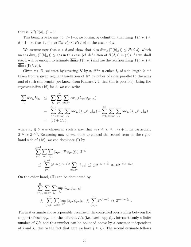
that is, Ht(Γ(h|K)) = 0.

This being true for any t > d+1−s, we obtain, by definition, that dimH(Γ(h|K)) ≤

d+ 1− s, that is, dimH(Γ(h|K)) ≤ H(d, s) in the case s ≤ d.

We assume now that s > d and show that also dimH(Γ(h|K)) ≤ H(d, s), which

means dimH(Γ(h|K)) ≤ d/s in this case (cf. definition of H(d, s) in (7)). As we shall

see, it will be enough to estimate dimB(Γ(h|K)) and use the relation dimH(Γ(h|K)) ≤

dimB(Γ(h|K)).

Given ν ∈ N, we start by covering K by ≈ 2νd/s n-cubes Iν of side length 2−ν/s

taken from a given regular tessellation of Rn by cubes of sides parallel to the axes

and of such side length (we know, from Remark 2.9, that this is possible). Using the

representation (16) for h, we can write

∑

Iν

oscIνh|K ≤∑

Iν

∞∑

j=1

∑

m∈Zn

oscIν(λjmψjm|K)

=

jν−1∑

j=1

∑

m∈Zn

∑

Iν

oscIν (λjmψjm|K) +∞∑

j=jν

∑

m∈Zn

∑

Iν

oscIν(λjmψjm|K)

=: (I) + (II),

where jν ∈ N was chosen in such a way that ν/s ≤ jν ≤ ν/s + 1. In particular,

2−jν ≈ 2−ν/s. Reasoning now as was done to control the second term on the right-

hand side of (18), we can dominate (I) by

jν−1∑

j=1

∑

m

∑

Iν

|λjm| |∇ψjm(ξν)| 2−jν

.

jν−1∑

j=1

2j−jν2(jν−j)d∑

m∈Zn

|λjm| . jν2−jν(s−d) ≈ ν2−ν(s−d)/s.

On the other hand, (II) can be dominated by

∞∑

j=jν

∑

m∈Zn

∑

Iν

supIν

|λjmψjm|K |

.

∞∑

j=jν

∑

m∈Zn

supRn

|λjmψjm|K | .

∞∑

j=jν

2−j(s−d) ≈ 2−ν(s−d)/s.

The first estimate above is possible because of the controlled overlapping between the

support of each ψjm and the different Iν ’s (i.e., each suppψjm intersects only a finite

number of Iν ’s and this number can be bounded above by a constant independent

of j and jν , due to the fact that here we have j ≥ jν). The second estimate follows

22

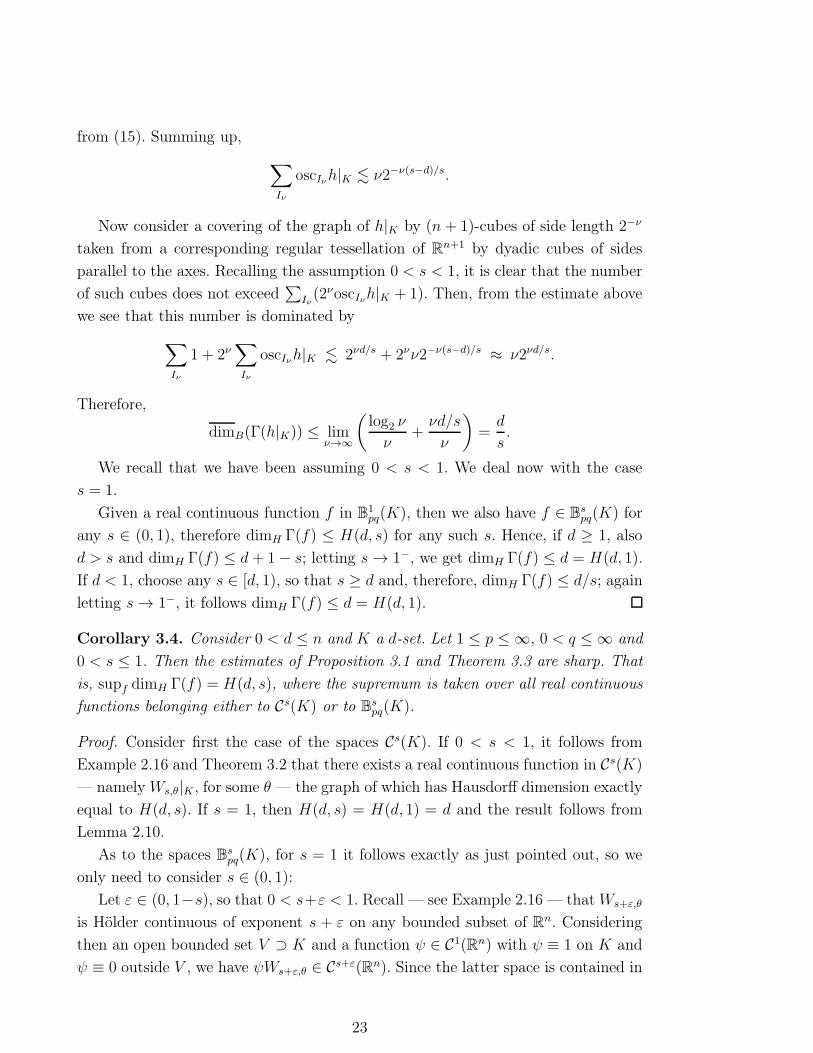
from (15). Summing up,

∑

Iν

oscIνh|K . ν2−ν(s−d)/s.

Now consider a covering of the graph of h|K by (n + 1)-cubes of side length 2−ν

taken from a corresponding regular tessellation of Rn+1 by dyadic cubes of sides

parallel to the axes. Recalling the assumption 0 < s < 1, it is clear that the number

of such cubes does not exceed∑

Iν(2νoscIνh|K + 1). Then, from the estimate above

we see that this number is dominated by

∑

Iν

1 + 2ν∑

Iν

oscIνh|K . 2νd/s + 2νν2−ν(s−d)/s ≈ ν2νd/s.

Therefore,

dimB(Γ(h|K)) ≤ limν→∞

(

log2 ν

ν+νd/s

ν

)

=d

s.

We recall that we have been assuming 0 < s < 1. We deal now with the case

s = 1.

Given a real continuous function f in B1pq(K), then we also have f ∈ B

spq(K) for

any s ∈ (0, 1), therefore dimH Γ(f) ≤ H(d, s) for any such s. Hence, if d ≥ 1, also

d > s and dimH Γ(f) ≤ d+ 1− s; letting s→ 1−, we get dimH Γ(f) ≤ d = H(d, 1).

If d < 1, choose any s ∈ [d, 1), so that s ≥ d and, therefore, dimH Γ(f) ≤ d/s; again

letting s→ 1−, it follows dimH Γ(f) ≤ d = H(d, 1).

Corollary 3.4. Consider 0 < d ≤ n and K a d-set. Let 1 ≤ p ≤ ∞, 0 < q ≤ ∞ and

0 < s ≤ 1. Then the estimates of Proposition 3.1 and Theorem 3.3 are sharp. That

is, supf dimH Γ(f) = H(d, s), where the supremum is taken over all real continuous

functions belonging either to Cs(K) or to Bspq(K).

Proof. Consider first the case of the spaces Cs(K). If 0 < s < 1, it follows from

Example 2.16 and Theorem 3.2 that there exists a real continuous function in Cs(K)

— namely Ws,θ|K , for some θ — the graph of which has Hausdorff dimension exactly

equal to H(d, s). If s = 1, then H(d, s) = H(d, 1) = d and the result follows from

Lemma 2.10.

As to the spaces Bspq(K), for s = 1 it follows exactly as just pointed out, so we

only need to consider s ∈ (0, 1):

Let ε ∈ (0, 1−s), so that 0 < s+ε < 1. Recall — see Example 2.16 — that Ws+ε,θ

is Hölder continuous of exponent s + ε on any bounded subset of Rn. Considering

then an open bounded set V ⊃ K and a function ψ ∈ C1(Rn) with ψ ≡ 1 on K and

ψ ≡ 0 outside V , we have ψWs+ε,θ ∈ Cs+ε(Rn). Since the latter space is contained in

23

Bs+ε∞∞(Rn) — cf. [12, pp. 4, 5 and 17] —, and this, in turn, is embedded in Bs

∞q(Rn),

then, using Remark 2.23, Definition 2.24 and Proposition 2.25, we can write

fε := Ws+ε,θ|K = (ψWs+ε,θ)|K = trK(ψWs+ε,θ) ∈ Bs∞q(K) ⊂ B

spq(K).

Therefore, given any ε ∈ (0, 1 − s) there exists a real continuous function fε ∈

Bspq(K) the graph of which has Hausdorff dimension equal to H(d, s+ ε). If s < d,

restrict further the ε to be also in (0, d − s), so that H(d, s + ε) = d + 1 − s − ε,

hence supfε dimH Γ(f) = d+ 1 − s = H(d, s). If s ≥ d, then also s+ ε ≥ d, so that

H(d, s+ ε) = d/(s+ ε), hence supfε dimH Γ(f) = d/s = H(d, s) too.

References

[1] M. Bricchi. Tailored function spaces and related h-sets. PhD thesis, Friedrich-

Schiller-Universität Jena, 2001.

[2] A. Carvalho. Box dimension, oscillation and smoothness in function spaces. J.

Funct. Spaces Appl., 3(3):287–320, 2005.

[3] A. Deliu and B. Jawerth. Geometrical dimension versus smoothness. Constr.

Approx., 8:211–222, 1992.

[4] K. J. Falconer. Fractal Geometry. John Wiley & Sons, Chichester, 1990.

[5] B. Hunt. The Hausdorff dimension of graphs of Weierstrass functions. Proc.

Amer. Math. Soc., 126:791–800, 1998.

[6] A. Jonsson and H. Wallin. Function Spaces on Subsets of Rn, volume 2 of Math.

Reports. Harwood Acad. Publ., 1984.

[7] J.-P. Kahane. Some random series of functions. Cambridge Univ. Press, 2nd

edition, 1985.

[8] A. Kamont and B. Wolnik. Wavelet Expansions and Fractal Dimensions. Con-

structive Approximation, 15(1):97–108, 1999.

[9] S. Moura. Function spaces of generalised smoothness. Dissertationes Math.,

398:88 pp., 2001.

[10] S. Moura. Function Spaces of Generalised Smoothness, Entropy Numbers, Ap-

plications. PhD thesis, University of Coimbra, 2001.

[11] F. Roueff. Dimension de Hausdorff du graphe d’une fonction continue: une

étude analytiqueet statistique. PhD thesis, Ecole Nat. Supér. Télécom., 2000.

24

[12] H. Triebel. Theory of Function Spaces II. Birkhäuser, Basel, 1992.

[13] H. Triebel. Fractals and Spectra. Birkhäuser, Basel, 1997.

[14] H. Triebel. Fractal analysis, an approach via function spaces. Jahresbericht

DMV, 104(4):171–199, 2002. English translation.

[15] H. Triebel. Theory of Function Spaces III. Birkhäuser, Basel, 2006.

25