arX

iv:1

004.

4911

v1 [

mat

h-ph

] 2

7 A

pr 2

010

ON EFFICIENCY OF HAMILTONIAN–BASED QUANTUM

COMPUTATION FOR LOW–RANK MATRICES

ZHENWEI CAO AND ALEXANDER ELGART

Abstract. We analyze a quantum evolution of the system where the problemHamiltonian HF is of small rank. We show the running time τ is boundedfrom below by O(

√

N), where N is a dimension of the Hilbert space. In aGedanken experiment, we construct an initial Hamiltonian and non–adiabatic

parametrization such that τ = O(√

N). We also prove that for a robustadiabatic computational device τ cannot be much smaller than O(N/ lnN).

1. Introduction and main results

1.1. Bounds on the running time in Hamiltonian–based quantum com-

putation. The Hamiltonian–based quantum computing model, known as the adi-abatic quantum computing (AQC), was proposed as an alternative to the standardcircuit model for implementing a quantum computer [5]. In the abstract setting,we are interested in finding the ground state of the given problem Hamiltonian HF ,in the shortest possible time. To this end, we consider a pair of hermitian N ×Nmatrices HI,F , for large values of N . Let H(s) be the interpolating Hamiltonian

H(s) := (1− f(s))HI + f(s)HF , (1.1)

where f is a monotone function on [0, 1] satisfying f(0) = 0, f(1) = 1. The idea ofthe adiabatic quantum computation (AQC) (e.g. [5]) is to prepare the initial stateof the system ψ(0) in a ground state ψI of the Hamiltonian HI , and let the systemevolve according to the (scaled) Schrodinger equation:

iψτ (s) = τH(s)ψτ (s) , ψτ (0) = ψI . (1.2)

The adiabatic theorem (AT) of quantum mechanics ensures that under certainconditions1 the evolution ψτ (1) of the initial state stays close to a ground state ofthe problem Hamiltonian HF . For AQC to be efficient, the running (i.e. physical)time τ in (1.2) must be much smaller than N . One then can ask what choice of theinitial Hamiltonian HI and the parametrization f(s) minimizes τ , and what theoptimal value of τ is.

One of the parameters that enters into the upper bound for τ in the standard ATis the minimal value g of the spectral gap g(s) between the ground state energy ofH(s) and the rest of its spectrum. Consequently, the traditional approach2 to AQCinvolves the estimation of g. Excluding a very short list of interesting situations forwhich g can be explicitly evaluated (e.g. [3]), it appears to be a hard problem. Insome instances one can get an idea of what size of g could be by using the first-orderperturbation theory (e.g. [11]).

1See Theorem 1.1 below.2We will discuss two exceptional results later on.

1

2 Z. CAO AND A. ELGART

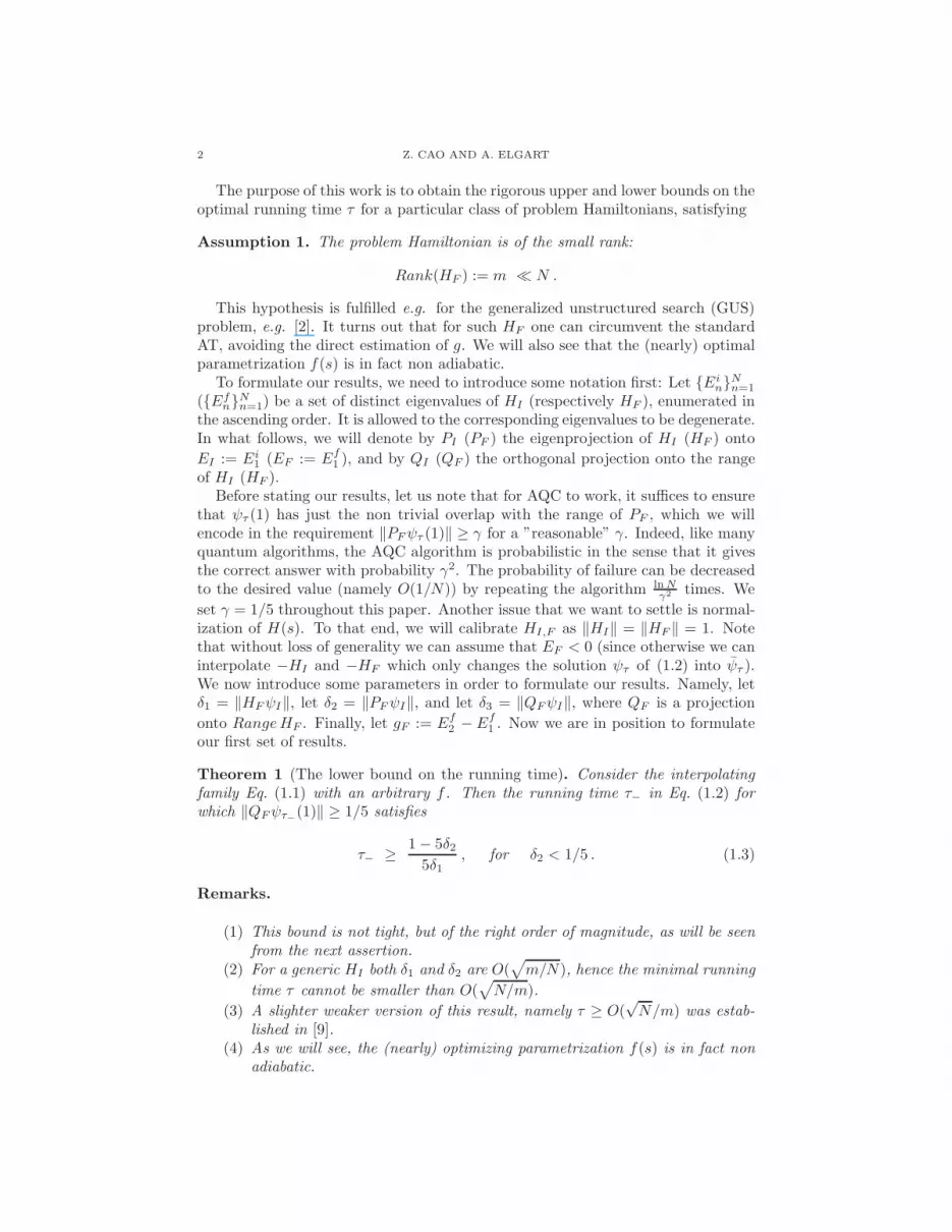
The purpose of this work is to obtain the rigorous upper and lower bounds on theoptimal running time τ for a particular class of problem Hamiltonians, satisfying

Assumption 1. The problem Hamiltonian is of the small rank:

Rank(HF ) := m ≪ N .

This hypothesis is fulfilled e.g. for the generalized unstructured search (GUS)problem, e.g. [2]. It turns out that for such HF one can circumvent the standardAT, avoiding the direct estimation of g. We will also see that the (nearly) optimalparametrization f(s) is in fact non adiabatic.

To formulate our results, we need to introduce some notation first: Let EinNn=1

(EfnNn=1) be a set of distinct eigenvalues of HI (respectively HF ), enumerated in

the ascending order. It is allowed to the corresponding eigenvalues to be degenerate.In what follows, we will denote by PI (PF ) the eigenprojection of HI (HF ) onto

EI := Ei1 (EF := Ef

1 ), and by QI (QF ) the orthogonal projection onto the rangeof HI (HF ).

Before stating our results, let us note that for AQC to work, it suffices to ensurethat ψτ (1) has just the non trivial overlap with the range of PF , which we willencode in the requirement ‖PFψτ (1)‖ ≥ γ for a ”reasonable” γ. Indeed, like manyquantum algorithms, the AQC algorithm is probabilistic in the sense that it givesthe correct answer with probability γ2. The probability of failure can be decreasedto the desired value (namely O(1/N)) by repeating the algorithm lnN

γ2 times. We

set γ = 1/5 throughout this paper. Another issue that we want to settle is normal-ization of H(s). To that end, we will calibrate HI,F as ‖HI‖ = ‖HF ‖ = 1. Notethat without loss of generality we can assume that EF < 0 (since otherwise we caninterpolate −HI and −HF which only changes the solution ψτ of (1.2) into ψτ ).We now introduce some parameters in order to formulate our results. Namely, letδ1 = ‖HFψI‖, let δ2 = ‖PFψI‖, and let δ3 = ‖QFψI‖, where QF is a projection

onto RangeHF . Finally, let gF := Ef2 − Ef

1 . Now we are in position to formulateour first set of results.

Theorem 1 (The lower bound on the running time). Consider the interpolatingfamily Eq. (1.1) with an arbitrary f . Then the running time τ− in Eq. (1.2) forwhich ‖QFψτ

−

(1)‖ ≥ 1/5 satisfies

τ− ≥ 1− 5δ25δ1

, for δ2 < 1/5 . (1.3)

Remarks.

(1) This bound is not tight, but of the right order of magnitude, as will be seenfrom the next assertion.

(2) For a generic HI both δ1 and δ2 are O(√

m/N), hence the minimal running

time τ cannot be smaller than O(√

N/m).

(3) A slighter weaker version of this result, namely τ ≥ O(√N/m) was estab-

lished in [9].(4) As we will see, the (nearly) optimizing parametrization f(s) is in fact non

adiabatic.

HAMILTONIAN–BASED QUANTUM COMPUTATION OF LOW–RANK MATRICES 3

Theorem 2 (The upper bound on the running time). There exists an explicit rankone HI and an explicit function f such that ‖PFψτ+(1)‖ ≥ 1/5 for

τ+ =C(1− EF )

|EF | δ2, (1.4)

for any C ∈ [1/3, 2/3], provided that δ3/gF = O(1/ lnN).

Remarks.

(1) For a generic choice of HI one has δ3 = O(√

m/N), δ2 = O(√

m1/N),where m1 is a dimension of the eigenspace of HF , associated with theeigenvalue EF . It implies that τ− and τ+ have roughly the same orderof magnitude, so that Theorem 1 and Theorem 2 provide fairly tight lowerand respectively upper bounds on the running time.

(2) This assertion can be viewed as an extension of the well known result [6]concerning the Grover’s search problem.

Note that a-priori the values of EF and δ2 may be unknown. For instance, thevalue of the overlap δ2 has to be determined in the GUS problem with the unknownnumber of marked items. To this end, we prove the following auxiliary result:

Theorem 3. Suppose that the value of EF is known. Then there is a Hamiltonian– based algorithm that determines δ2 with 1/N2 accuracy and requires O((lnN)2)of the running time.

Remark. The running time for this sub-algorithm is much shorter than τ+, so itdoes not significantly affect the total running time. A parallel result in the context ofthe quantum circuit model was establishes earlier in [2], although the corresponding

algorithm runs for much longer (roughly O(√N)) time.

1.2. Gaps in the spectrum of the interpolating Hamiltonian. Although thesize of the gap in the spectrum of H(s) did not play much of the role so far, it isinstructive to estimate it for the following reason: The size of the gap manifestsitself in the adiabatic theorem of quantum mechanics (AT), on which AQC is build.To formulate AT precisely, we need to introduce some notation first:

Definition. We say that the family H(s) is k–admissible if the eigenvalue λ1(s)is separated by a uniform gap g(k) > 0 from the eigenvalues λn(s)Nn=k+1 for alls ∈ [0, 1], that is

mins∈[0,1]

(λk+1(s) − λ1(s)) = g(k) . (1.5)

The following assertion holds for such a family, see e.g. [1]:

Theorem 1.1 (Adiabatic theorem). If the family H(s) is k–admissible, then thesolution ψτ (s) of the IVP (1.2) satisfies

limτ→∞

dist(

ψτ (1), Range P(k))

= 0 , (1.6)

where P (k) is a spectral projection of HF onto the eigenvalues Efnkn=1.

To AQC to be meaningful, one should choose the initial Hamiltonian HI in sucha way that Rank PI is small. It is important to note that Theorem 1.1 allows tohave the level crossings (or the avoided crossings) for λ1(s) with other first k − 1eigenvalues of H(s). Let g := g(1), then the error in the adiabatic evolution for

4 Z. CAO AND A. ELGART

1-admissible family depends on the size of the gap g, with the rough upper boundon the error of the form C

τg3 [10].

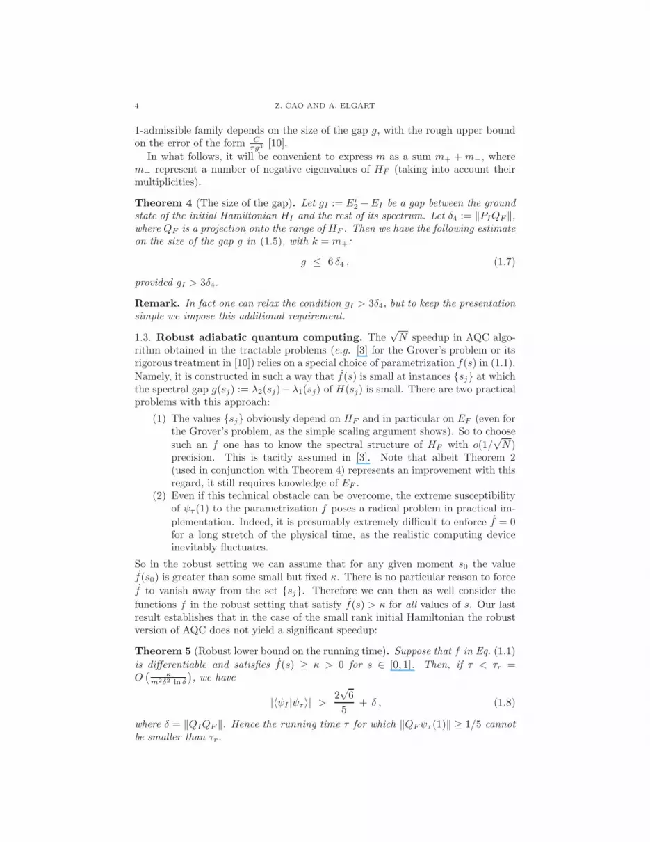
In what follows, it will be convenient to express m as a sum m+ +m−, wherem+ represent a number of negative eigenvalues of HF (taking into account theirmultiplicities).

Theorem 4 (The size of the gap). Let gI := Ei2 −EI be a gap between the ground

state of the initial Hamiltonian HI and the rest of its spectrum. Let δ4 := ‖PIQF‖,where QF is a projection onto the range of HF . Then we have the following estimateon the size of the gap g in (1.5), with k = m+:

g ≤ 6 δ4 , (1.7)

provided gI > 3δ4.

Remark. In fact one can relax the condition gI > 3δ4, but to keep the presentationsimple we impose this additional requirement.

1.3. Robust adiabatic quantum computing. The√N speedup in AQC algo-

rithm obtained in the tractable problems (e.g. [3] for the Grover’s problem or itsrigorous treatment in [10]) relies on a special choice of parametrization f(s) in (1.1).

Namely, it is constructed in such a way that f(s) is small at instances sj at whichthe spectral gap g(sj) := λ2(sj)−λ1(sj) of H(sj) is small. There are two practicalproblems with this approach:

(1) The values sj obviously depend on HF and in particular on EF (even forthe Grover’s problem, as the simple scaling argument shows). So to choose

such an f one has to know the spectral structure of HF with o(1/√N)

precision. This is tacitly assumed in [3]. Note that albeit Theorem 2(used in conjunction with Theorem 4) represents an improvement with thisregard, it still requires knowledge of EF .

(2) Even if this technical obstacle can be overcome, the extreme susceptibilityof ψτ (1) to the parametrization f poses a radical problem in practical im-

plementation. Indeed, it is presumably extremely difficult to enforce f = 0for a long stretch of the physical time, as the realistic computing deviceinevitably fluctuates.

So in the robust setting we can assume that for any given moment s0 the valuef(s0) is greater than some small but fixed κ. There is no particular reason to force

f to vanish away from the set sj. Therefore we can then as well consider the

functions f in the robust setting that satisfy f(s) > κ for all values of s. Our lastresult establishes that in the case of the small rank initial Hamiltonian the robustversion of AQC does not yield a significant speedup:

Theorem 5 (Robust lower bound on the running time). Suppose that f in Eq. (1.1)

is differentiable and satisfies f(s) ≥ κ > 0 for s ∈ [0, 1]. Then, if τ < τr =O(

κm2δ2 ln δ

), we have

|〈ψI |ψτ 〉| >2√6

5+ δ , (1.8)

where δ = ‖QIQF ‖. Hence the running time τ for which ‖QFψτ (1)‖ ≥ 1/5 cannotbe smaller than τr.

HAMILTONIAN–BASED QUANTUM COMPUTATION OF LOW–RANK MATRICES 5

Remark. This theorem tells us that for a generic HI of the small rank the robustrunning time τr cannot be smaller than O(N/ lnN). Hence AQC is not much betterthan its classical counterpart that solves GUS for τ = O(N).

2. Proof of Theorem 1

For a solution ψτ (s) of (1.2), let

φτ (s) := eifτ (s)ψτ (s) , fτ (s) = τ EI

∫ s

0

(1− g(r)) dr . (2.1)

Then one can readily check that φτ (s) satisfies the IVP

iφτ (s) = τH(s)ψτ (s) , φτ (0) = ψI , (2.2)

where

H(s) = (1− f(s)) (HI − EI I) + f(s)HF .

The factor eifτ (s) is usually referred to as a dynamical phase.Let Uτ (t, s) be a semigroup generated by H(s), namely

− i ∂sUτ (t, s) = τ Uτ (t, s)H(s) ; Uτ (s, s) = I ; t ≥ s . (2.3)

Then the solution φτ (1) of (2.2) is equal to Uτ (1, 0)ψI . On the other hand,

I − Uτ (1, 0) =

∫ 1

0

∂s Uτ (1, s) ds = i τ

∫ 1

0

Uτ (t, s)H(s) ds ,

hence applying both sides on ψI we obtain

ψI − φτ (1) = i τ

∫ 1

0

Uτ (t, s)H(s)ψI ds .

We infer

‖ψI − φτ (1)‖ ≤ τ

∫ 1

0

‖H(s)ψI‖ ds .

But

H(s)ψI = (1− f(s)) (HI − EI I) + f(s)HF ψI = f(s)HFψI ,

and we get the bound

‖ψI − φτ (1)‖ ≤ τ δ1

∫ 1

0

f(s) ds ≤ τ δ1 ,

where in the last step we used 0 ≤ f(s) ≤ 1. Clearly,∣∣∣‖QFψI‖ − ‖QFφτ (1)‖

∣∣∣ ≤ ‖QFψI − QFφτ (1)‖ ≤ ‖ψI − φτ (1)‖ ≤ τ δ1 ,

so that

‖QFφτ (1)‖ ≤ τ δ1 + δ2 .

On the other hand, by the assumption of the theorem ‖QFψτ (1)‖ ≥ 1/2, hence‖QFφτ (1)‖ ≥ 1/2. As a result, we can bound

1/5 ≤ τ δ1 + δ2 ,

and the assertion follows.

6 Z. CAO AND A. ELGART

3. Proof of Theorem 2

We will choose HI = −|ψI〉〈ψI |, and a non adiabatic parametrization

f(s) =

0 , s = 0

α ≡ 11−EF

, s ∈ (0, 1)

1 , s = 1

That means we move extremely quickly (instantly in fact) to the middle of thepath, stay there for the time τ , and then move quickly again to the end of the path.We first observe that regardless of the choice of f(s) in (1.1) we have ψτ (s) ∈ Y ,where Y is a subspace of the Hilbert space, spanned by the vectors in the range ofHF and ψI . Here we have used the fact that the range of HI by the assumptionof the theorem coincides with SpanψI. Let us choose the orthonormal basiseim+1

i=1 for Y as follows: The first m vectors in the basis are the eigenvectors

of HF corresponding to Efi that differ from zero, and the last vector em+1 is

obtained from ψI using the Gram Schmidt procedure. That is,

em+1 :=QFψI

‖QFψI‖=

QFψI√

1− δ23, QF = 1−QF .

We then have

‖em+1 − ψI‖2 = ‖QF em+1 −QFψI‖2 + ‖QF em+1 − QFψI‖2

= δ23 +

(

1√

1− δ23− 1

)2(1− δ23

)

≤ δ23 + δ43 . (3.1)

Our choice of g ensures that

ψτ (1) = e−iατ ·(EFPI +HF )ψI .

Here we introduce PF as the orthogonal projection onto the span of ei with

Efi = Ef

1 , and Pm+1 the orthogonal projection onto em+1. Clearly

Pm+1 =QF PI QF

1− δ23

We want to compute the matrix elements of the propagator e−iατ(HI +HF ) in thebasis ei. To this end, we observe that in this basis HF = diag(EF , . . . , E

fm, 0),

and HI is a block matrix such that∥∥∥∥EFPI −

[0 δ3 V

∗

δ3 V EF

]∥∥∥∥

≤ 3δ23 |EF | , (3.2)

where ‖V ‖ = |EF |. Indeed, we have

‖QF PI QF ‖ = δ23 ,

‖Pm+1 PI Pm+1‖ = 1− δ23 ,

‖Pm+1 PI QF ‖ = δ3 (1 − δ23)1/2 .

Together, we obtain that in this basis∥∥∥∥EFPI + HF −

[D δ3 V

∗

δ3 V EF

]∥∥∥∥

≤ 3δ23 |EF | ,

HAMILTONIAN–BASED QUANTUM COMPUTATION OF LOW–RANK MATRICES 7

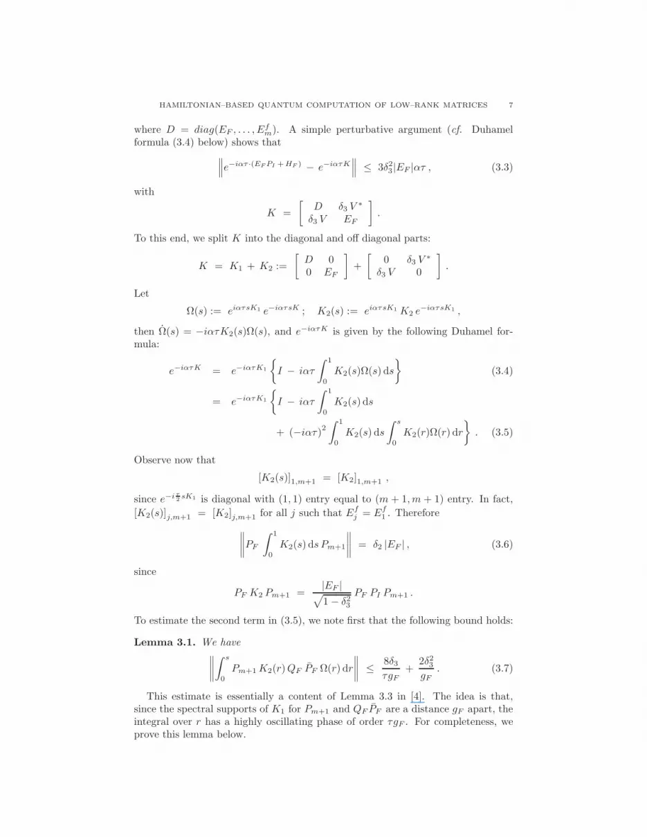
where D = diag(EF , . . . , Efm). A simple perturbative argument (cf. Duhamel

formula (3.4) below) shows that∥∥∥e−iατ ·(EFPI +HF ) − e−iατK

∥∥∥ ≤ 3δ23 |EF |ατ , (3.3)

with

K =

[D δ3 V

∗

δ3 V EF

]

.

To this end, we split K into the diagonal and off diagonal parts:

K = K1 + K2 :=

[D 00 EF

]

+

[0 δ3 V

∗

δ3 V 0

]

.

Let

Ω(s) := eiατsK1 e−iατsK ; K2(s) := eiατsK1 K2 e−iατsK1 ,

then Ω(s) = −iατK2(s)Ω(s), and e−iατK is given by the following Duhamel for-mula:

e−iατK = e−iατK1

I − iατ

∫ 1

0

K2(s)Ω(s) ds

(3.4)

= e−iατK1

I − iατ

∫ 1

0

K2(s) ds

+ (−iατ)2∫ 1

0

K2(s) ds

∫ s

0

K2(r)Ω(r) dr

. (3.5)

Observe now that

[K2(s)]1,m+1 = [K2]1,m+1 ,

since e−i τ2sK1 is diagonal with (1, 1) entry equal to (m + 1,m + 1) entry. In fact,

[K2(s)]j,m+1 = [K2]j,m+1 for all j such that Efj = Ef

1 . Therefore

∥∥∥∥PF

∫ 1

0

K2(s) ds Pm+1

∥∥∥∥

= δ2 |EF | , (3.6)

since

PF K2 Pm+1 =|EF |

√

1− δ23PF PI Pm+1 .

To estimate the second term in (3.5), we note first that the following bound holds:

Lemma 3.1. We have∥∥∥∥

∫ s

0

Pm+1K2(r)QF PF Ω(r) dr

∥∥∥∥

≤ 8δ3τgF

+2δ23gF

. (3.7)

This estimate is essentially a content of Lemma 3.3 in [4]. The idea is that,since the spectral supports of K1 for Pm+1 and QF PF are a distance gF apart, theintegral over r has a highly oscillating phase of order τgF . For completeness, weprove this lemma below.

8 Z. CAO AND A. ELGART

Armed with this estimate and using the fact that K2(s) is off diagonal, we get∥∥∥∥PF

∫ 1

0

K2(s) ds

∫ s

0

K2(r)Ω(r) dr Pm+1

∥∥∥∥

= ‖PF K2 Pm+1‖ ·∥∥∥∥Pm+1

∫ 1

0

ds

∫ s

0

K2(r)Ω(r) dr Pm+1

∥∥∥∥

≤ |EF | δ2 ·∫ 1

0

ds

∥∥∥∥

∫ s

0

Pm+1K2(r)(PF +QF PF )Ω(r)Pm+1dr

∥∥∥∥

≤ |EF | δ2 ·∫ 1

0

‖Pm+1K2(r)PF ‖ dr

+ maxs∈[0,1]

∥∥∥∥

∫ s

0

Pm+1K2(r)QF PF Ω(r) dr

∥∥∥∥

,

where we have used ‖Ω(r)‖ = ‖Pm+1‖ = 1 and (3.6). Applying the estimate (3.6)and (3.7), we bound

‖PF

∫ 1

0

K2(s) ds

∫ s

0

K2(r)Ω(r) dr Pm+1

∥∥∥∥

(3.8)

≤ |EF | δ2 ·

|EF | δ2 +8δ3τgF

+2δ23gF

.

Multiplying (3.5) by PF from the left and by Pm+1 from the right, and using theestimates (3.6) and (3.9), we establish

∥∥PF e

−iατK Pm+1

∥∥ ≥ ατ

∥∥∥∥PF

∫ 1

0

K2(s) ds Pm+1

∥∥∥∥

− (ατ)2∥∥∥∥PF

∫ 1

0

K2(s) ds

∫ s

0

K2(r)Ω(r) dr Pm+1

∥∥∥∥

= ατ |EF | δ2 ·(

1 − ατ ·

|EF |δ2 +8δ3τgF

+2δ23gF

)

. (3.9)

Combining the estimates in (3.1), (3.3), and (3.9), the result will follow provided

ατ |EF | δ2 ·(

1 − ατ ·

|EF |δ2 +8δ3τgF

+2δ23gF

)

≥ 1/5 + δ23 + δ43 + 3δ23 |EF |ατ .

Note now that for τ = O(1/δ2) the above inequality is satisfied for values of τ andδ3 such that

ατ |EF | δ2 · (1 − ατ |EF |δ2 ) ≥ 2/9 , δ3/gF = O(1/ lnN) .

The result now follows.

Proof of Lemma 3.1. Let

X :=1

2πi

∮

Γ

Pm+1 (K1 − zI)−1K2 (K1 − zI)−1QF PF d z , (3.10)

where the contour Γ is a circle z ∈ C : |z − EF | = gF /2. Since1

2πi

∮

Γ

(K1 − zI)−1 d z = PF + Pm+1 ,

one can readily check that

[X , K1] = Pm+1 K2QF PF .

HAMILTONIAN–BASED QUANTUM COMPUTATION OF LOW–RANK MATRICES 9

Hence∫ s

0

Pm+1K2(r)QF PF Ω(r) dr =−2i

τ

∫ s

0

d

dr

(

e−i τ2rK1 X ei

τ2rK1

)

Ω(r) dr .

Integrating the right hand side by parts, we obtain∫ s

0

Pm+1K2(r)QF PF Ω(r) dr

= −2i

τ

e−i τ2rK1 X ei

τ2rK1 Ω(r)

∣∣∣

s

0−∫ s

0

e−i τ2sK1 X ei

τ2sK1 Ω(r) dr

= −2i

τe−i τ

2rK1 X ei

τ2rK1 Ω(r)

∣∣∣

s

0−∫ s

0

e−i τ2sK1 X ei

τ2sK1 K2(r)Ω(r) dr .

The first term is bounded in norm by 4 ‖X‖τ , while the second one is bounded

by ‖X‖ · ‖K2‖. It follows from (3.10) that ‖X‖ ≤ 2‖K2‖gF

. On the other hand,

‖K2‖ = δ3‖V ‖ = |EF |δ3 ≤ δ3 by (3.2), and the result follows.

4. proof of theorem 3

The starting point is a pair of identities, [7]:

e−p∞∑

k=1

pk sin(kω)

k!= ep(cosω−1) sin(p sinω)

e−p∞∑

k=1

pk cos(kω)

k!= ep(cosω−1) cos(p sinω) . (4.1)

In particular, if 1 − cosω > g, each term in Eq. (4.1) is bounded by e−pg andtherefore is smaller than 1/N2 provided p = 2 lnN/g. On the other hand, theremainders to the partial sums (up to k = L) in Eq. (4.1) are O(pL/L!) providedthe latter quantity is small. Combining these observations, we get

e−p

p∑

k=1

pkeikω

k!=

1 +O(1/N2) , ω = 0

O(1/N2) , 1− cosω > g,

for p = 2 lnN/g and g < 1. Hence

e−p

p∑

t=1

pk

k!〈ψI |eit(HF−EF )ψI〉 = (δ2)

2 +O(1/N2) , (4.2)

for p = 2 lnN/(1− cos gF ). The total running time is∑p

t=1 t = O((lnN)2).

5. Proof of Theorem 4

The main tool we are going to use is the so called Krein’s formula for the rankm perturbation of the initial Hamiltonian HI . It gives a characterization of thelocation of m eigenvalues of the perturbed matrix that differ from the spectralvalues of HI . Specifically, let A,B be two hermitian matrices, with Rank B = m,and let Q be an orthogonal projection onto Range B. Suppose that A is invertible(that is 0 /∈ σ(A)). Then 0 is an eigenvalue of A + tB if and only if the m × mmatrix K−1 + tBQ contains 0 in its spectrum, with

K := QA−1Q .

10 Z. CAO AND A. ELGART

K−1 + tBQ is interpreted as acting in the m–dimensional space Range B. TheKrein’s formula follows directly from the Schur complement formula, which saysthat if C is invertible then

QC−1Q =(QCQ − QCQ (QCQ)−1 QCQ

)−1,

where Q := I −Q and the inverses on the right hand side are understood as actingon the ranges of Q and Q, respectively.

To apply the Krein’s formula in our context, we form a one parameter family

Ht := HI + tHF , t =s

1− s, t ∈ [0,∞) .

It is then follows that for a fixed t ∈ (0,∞) the eigenvalues of Ht that differ fromσ(HI) are given by the roots of the equation

det(K−1(E) + tHFQF

)= 0 , (5.1)

whereK(E) := QF (HI − E)−1QF .

Whenever it is clear from the context that we are working with the operators onRange QF , we will suppress the QF dependence.

To analyze (5.1), we start with the following simple observation:

Lemma 5.1. The matrix K(E) can be decomposed as

K(E) = K(E) +δ24 D

EI − E. (5.2)

Here the matrix D is positive semi-definite, and is bounded in norm by 1. Thematrix K(E) is holomorphic in the half plane Re E > EI − gI/2 and is positivedefinite for E ∈ [EI − gI/2, EI + gI/2]. Moreover, in this interval we have bounds

2

4 + gI− δ24 ≤ K(E) ≤ 2

gI;

4

(4 + gI)2− δ24 ≤ dK(E)

dE≤ 4

g2I. (5.3)

Proof. We decompose

K(E) = QF (HI − E)−1QF = QF PI (HI − E)

−1QF +QFPI (HI − E)

−1QF .

The first contribution will correspond to K(E) in (5.3), and the second one to itscounterpart in (5.3). Note now that for E ∈ [EI − gI/2, EI + gI/2] we have

gI2PI ≤ PI(HI − E) ≤

(

2 +gI2

)

PI ,

where the the upper bound is a consequence of ‖HI‖ = 1. Hence we obtain

2

4 + gIQF PIQF ≤ QF PI(HI − E)−1QF ≤ 2

gIQF PIQF .

Therefore, the first bound in (5.3) follow now from

QF PIQF = QF − QFPIQF

and0 ≤ QFPIQF ≤ δ24 QF .

To obtain the second bound in (5.3) we note that

d

dE(HI − E)

−1= (HI − E)

−2

for E /∈ σ(HI), and then proceed as above.

HAMILTONIAN–BASED QUANTUM COMPUTATION OF LOW–RANK MATRICES 11

In applications to the AQC the parameter δ4 is typically extremely small: δ24 =O(1/N). Hence the second contribution in (5.2) is small provided |E − EI | ≫ δ4.

Therefore for value of E in such intervals, we can first find the roots Ei(t) of

det(

K−1(E) + tHF

)

= 0 , (5.4)

and then estimate |Ei(t)−Ei(t)|, where Ei(t) are corresponding roots of (5.1). Aswe will see, the level crossings or the avoided level crossings for Ht occur for valuesof t such that a pair of eigenvalues Ek(t), El(t) is close to EI . To find these valuesof t in the first approximation, we fix the value E = EI in (5.4) and solve it for t.We have

Lemma 5.2. The equation

det(

K−1(EI) + tHF

)

= 0 , (5.5)

has exactly m+ roots tjm+

j=1 on (0,∞), where m+ is a number of negative eigen-values of HF .

Proof. Let A := K(EI), then it follows from previous lemma that 0 < A. Hence

(A−1 + tHF

)= tA−1/2

(

t−1 + A1/2HFA1/2)

A−1/2 .

The right hand side is not invertible for values tj such that

−t−1j ∈ σ

(

A1/2HFA1/2)

,

and the result follows now from Sylvester’s law of inertia [8].

We are now in position to estimate the size of the gap g from above. Namely,we consider the gaps gj for Ht for t = tj . Since t =

s1−s and H(s) = (1 − s)Ht, we

obtain g ≤ gj1+tj

≤ gj . Let

β := 2

(

δ244

(4+gI )2− δ24

)1/2

.

To get a bound on gj we show that (5.1) has a roots in the intervals [EI−β,EI) and(EI , EI + β], at t = tj . We then infer that gj ≤ 2β, from which the upper boundin (1.7) follows since β < 3δ4. Observe first that by condition of the Theorem 4,σ(HI) ∩ [EI − β,EI) = ∅, hence we are in position to use Lemma 5.1. We onlyshow that for the first interval, the proof is analogous for the second one.

To this end, we will denote by sgn(A) the signature of the matrix A. We observe

that sinceδ24 DEI−E in (5.2) is positive semidefinite and monotone increasing for the

values of E in [EI − β,EI), we have

sgn(K−1(EI + 0) + tjHF ) ≤ sgn(K−1(EI) + tjHF ) . (5.6)

On the other hand, we have

K(EI) − K(EI − β) =

∫ EI

EI−β

K ′(E) dE ≥ β

(4

(4 + gI)2− δ24

)

, (5.7)

12 Z. CAO AND A. ELGART

where in the last step we have used (5.3). Hence

K(EI − β) = K(EI − β) +δ24 D

β

≤ K(EI) −(

β

(4

(4 + gI)2− δ24

)

I − δ24 D

β

)

(5.8)

≤ K(EI) − δ24βI < K(EI) ,

with a choice of β as above, and where we use ‖D‖ ≤ 1. We infer

K−1(EI − β) + tjHF > K−1(EI) + tjHF ,

and since the matrix K−1(EI) + tjHF has zero eigenvalue by construction, weobtain

sgn(K−1(EI − β) + tjHF ) < sgn(K−1(EI) + tjHF ) . (5.9)

Combining (5.6) and (5.9) together, we get

sgn(K−1(EI − β) + tjHF ) < sgn(K−1(EI + 0) + tjHF ) . (5.10)

But the family K−1(E) + tjHF is continuous on [EI − β,EI), hence there shouldbe some value of E in this interval for which K−1(E) + tjHF has the eigenvalue0.

6. proof of theorem 5

LetB(s) = (f(s)HF − ((1− f(s))EI + ǫi))−1 ,

and let φ(s) = ψI − f(s)HFB(s)ψI , where ǫ is a small parameter to be chosenlater. Omitting the s dependence, we have

Hφ = −f(1− f)HIHFB ψI + iǫfHFB ψI . (6.1)

That means that away from the m values of s for which B(s) has zero eigenvalue,

‖Hφ‖ is very small, since ‖HIHFψI‖ ≤ δ2. Note now that

〈φ(1)|φτ (1)〉 = 〈φ(0)|φτ (0)〉 +

∫ 1

0

d

ds〈φ(s)|φτ (s)〉 ds , (6.2)

where φτ (s) is defined in (2.1). But 〈φ(0)|φτ (0)〉 = 1 and

|〈φ(1)|φτ (1)〉| =

∣∣∣∣〈ψI |φτ (1)〉 − 〈ψI |

HF

HF − ǫ i|φτ (1)〉

∣∣∣∣

≤ |〈ψI |φτ (1)〉| + ‖QFψI‖ ≤ |〈ψI |φτ (1)〉| + δ .

Substitution into Eq. (6.2) gives

1 − |〈ψI |φτ (1)〉| ≤∣∣∣∣

∫ 1

0

d

ds〈φ(s)|φτ (s)〉 ds

∣∣∣∣+ δ .

Hence Eq. (1.8) will follow if∣∣∣∣

∫ 1

0

d

ds〈φ(s)|φτ (s)〉 ds

∣∣∣∣< 1 − 2

√6

5− 2δ . (6.3)

We haved

ds〈φ(s)|φτ (s)〉 = 〈φ(s)|φτ (s)〉 − iτ〈φ(s)|H(s)|φτ (s)〉 .

HAMILTONIAN–BASED QUANTUM COMPUTATION OF LOW–RANK MATRICES 13

We bound the first term on the right hand side by ‖φ‖ and the second one by

τ‖Hφτ‖. A straightforward computation (using Eq. (6.1) for the second term)shows that

‖φ‖ ≤ fδ

∆ǫ+

2fδ

(∆ǫ)2 ; ‖Hφτ‖ ≤ δ2 + ǫδ

∆ǫ,

where ∆ǫ(s) := dist(f(s)σ(HF ) , (1−f(s))EI+ǫ i). Here dist(S, z) is an Euclideandistance from the set S to the point z in C, and σ(H) stands for the spectrum ofH .

As a result, we obtain a bound∣∣∣∣∣

˙︷ ︸︸ ︷

〈φ|φτ 〉∣∣∣∣∣≤ (f + τδ + τǫ)

δ

∆ǫ+ 2

f δ

(∆ǫ)2 .

Integrating both sides over s and using the bounds∫ 1

0

fds

∆ǫ(s)≤ −2m ln ǫ ;

∫ 1

0

fds

(∆ǫ(s))2 ≤ 2m

ǫ;

∫ 1

0

ds

∆ǫ(s)≤ −2m

ln ǫ

κ,

we can estimate∣∣∣∣

∫ 1

0

d

ds〈φ(s)|φτ (s)〉 ds

∣∣∣∣≤ 2mδ

(

− ln ǫ

(

1 +τδ

κ+τǫ

κ

)

+2

ǫ

)

.

Hence the required bound in Eq. (6.3) follows with the choice ǫ = 10−3mδ, providedτ ≤ − Cκ

ǫ2 ln ǫ where C is a constant.

Acknowledgment: This work was supported in part by NSF grant DMS–0907165.

References

[1] J. E. Avron and A. Elgart. Adiabatic theorem without a gap condition. Comm. Math. Phys.,203, 445–463 (1999)

[2] G. Brassard, P. Hoyer, and A. Tapp. Quantum Counting. Lecture Notes in Comput. Sci.,1444, 820–831, Springer-Verlag, New York/Berlin (1998)

[3] W. van Dam, M. Mosca, and U. Vazirani. How powerful is adiabatic quantum computation?,in 42nd IEEE Symposium on Foundations of Computer Science, 279-287 (2001)

[4] A. Elgart and J. H. Schenker A strong operator topology adiabatic theorem. Rev. Math.

Phys., 14, 569–584 (2002)[5] E. Farhi, J. Goldstone, S. Gutmann, J. Lapan, A. Lundgren, and D. Preda. A quantum adia-

batic evolution algorithm applied to random instances of an NP-complete problem, Science,292, 472–476 (2001)

[6] E. Farhi and S. Gutmann. An Analog Analogue of a Digital Quantum Computation, Phys.Rev. A. 57, 2403–2406 (1998)

[7] I. S. Gradshteyn and I. M. Ryzhik, formulae (1.449), Table of integrals, series, and products

(Elsevier/Academic Press, Amsterdam, 2007)[8] R. Horn and C. Johnson, Matrix analysis. Cambridge University Press, Cambridge (1990)[9] L. M. Inannou and M. Mosca, Int. J. Quant. Inform. 6, 419 (2008).

[10] S. Jansen, M. B. Ruskai, and R. Seiler, J. Math. Phys., 48, 102111–102126 (2007)[11] A. Tulsi. Adiabatic quantum computation with a one-dimensional projector Hamiltonian.

Phys. Rev. A, 80, 219–253, (2009)

E-mail address: zhenwei@math.vt.edu

E-mail address: aelgart@vt.edu

Department of Mathematics, Virginia Tech., Blacksburg, VA, 24061