arX

iv:m

ath/

0406

621v

2 [

mat

h.D

S] 1

6 A

ug 2

004

On the Degree Growth of Birational Mappings

in Higher Dimension

Eric Bedford and Kyounghee Kim

§0. Introduction

Let f : Cd → Cd be a birational map. The problem of determining the behavior of theiterates fn = f · · · f is very interesting but not well understood. A basic property ofa rational map is its degree (see §1 for the definition). Another quantity is the dynamicaldegree

δ(f) = limn→∞

(deg(fn))1n

which is invariant under birational self-maps of Cd (see [BV]). It has been called “com-plexity” by some physicists (see [BM] and [AABM]), and its logarithm has been called“algebraic entropy” in [BV].

One aspect of a birational map is that its birational conjugacy class does not have awell-defined “domain.” Namely, if f : X → X is a (birational) dynamical system, thenany birational equivalence h : X → X will convert f to a (birational) dynamical systemon f = h f h−1 : X → X. This may serve as a significant change of the presentationof f , since the cohomology groups of X and X may have different dimensions. Thereis a well-defined pull-back map on cohomology f∗ : H1,1(X) → H1,1(X). Thus we candefine δ(f) more generally as limn→∞ ||(fn)∗||1/n, which is the exponential rate of growthof the action of fn on H1,1. Dinh and Sibony [DS] showed that this more general δ(f) isbirationally invariant.

The passage to cohomology may or may not be compatible with the dynamical system,depending on whether (f∗)n = (fn)∗ holds on H1,1. In case this holds, we say that f isH1,1-regular, or simply 1-regular. And if f is 1-regular, then it follows that δ is thespectral radius of f∗. We will pursue the study of δ using what might be called a methodof regularization. The first step of this method is to replace the pair (f, X) by a regular pair(f , X). This is done by finding a new complex manifold X which is birationally equivalentto X . The second step, then, is to determine f∗ and its spectral radius.

In this paper, we show how the method of regularization may be carried out on certainsub-classes of the family of maps which have the form f = L J , where L is an invertiblelinear map, and J(x1, . . . , xd) = (x−1

1 , . . . , x−1d ). Generally speaking, a birational map

has subvarieties that are mapped to lower dimensional sets, and it has lower dimensionalsubvarieties that are blown up to sets of higher dimension. In the case of f = L J , thecoordinate hypersurfaces xj = 0 are blown down to points, and the points eℓ = [0 :. . . : 1 : . . . : 0] are blown back up to hypersurfaces. This interplay between the blowingdown and the blowing up serves as the key for degree growth. The essential objects arethose orbits of the following form: xj = 0 → ∗ → · · · → ∗ → eℓ. That is, they startat a hypersurface which is blown down to a point, and the orbit of this point lands ona point of indeterminacy which is blown back up to a hypersurface. We say that suchorbits are singular. In §4 we define the class of elementary maps, which are characterizedby the property that they are locally biholomorphic at the intermediate points of singularorbits. The 1-regularization of an elementary map is obtained by blowing up the points

1

of the singular orbits. The singular orbits of an elementary map can be organized intoan orbit list structure Lc, Lo, which consists of two sets of lists of positive integers. It isthen shown how δ = δ(Lc,Lo) is determined by this list structure: an expression for f∗ isgiven in §4, and the characteristic polynomial is given in the Appendix. In §7 we illustratethis method by carrying out the procedure of finding orbit lists for some maps that haveappeared in the mathematical physics literature.

In general we have δ ≤ deg(f), and the existence of a singular orbit causes theinequality to be strict (Theorem 4.2). It is often desirable to have some way of estimatingδ without actually computing it. To this end, we give a way of comparing δ for two mapsf and f with list structures Lc, Lo and Lc, Lo, respectively. In §5 we give a number ofcomparison results; here are two examples. Theorem 5.1 shows that if f and f have thesame list structures, except that the orbits of f are longer, then δ(f) ≤ δ(f). In Theorem5.3, we show that adding a complete orbit list decreases δ. If we simply add a new singularorbit of length M to one of the orbit lists, then whether δ is increased or decreased dependson the size of M .

In §6 we introduce linear maps Lp, which are determined by a permutation p. Therest of §6 will be devoted to a consideration of the case where p = I is the identitypermmutation. The maps f = LI J are the Noetherian maps which were defined in thework [BHM]. Our primary motivation in this section is to show how the work of §4 appliesto give deg(fn), n ≥ 0 for these maps. These same numbers were conjectured in [BHM].

For more general permutations p, the map fp = Lp J can lead to some complicatedexamples of orbit collision. The expression orbit collision refers to the fact that a singularorbit xj = 0 → ∗ → . . .→ σk → . . .→ eℓ can contain a point σk ∈ xk = 0−I where fis smooth but not locally invertible. Thus the singular orbit starting at xj = 0 containsthe singular orbit starting at xk = 0 (and possibly others). In §8 we define singularchains. The singular chain structure is used both to construct the 1-regularization (fX , X)of (fp,P) and to write down f∗

X . As before, δ(fp) is given by the spectral radius of f∗X .

In this paper we follow up on ideas of Diller and Favre [DF], Guedj [G] and Boukraa,Hassani and Maillard [BHM]. The paper [DF] shows that 1-regularization is possible for allbirational maps in dimension two, and this forms the basis for their penetrating analysis.The possibility of extending this approach to the case of higher dimension was discussed in[BHM]. Birational maps are more complicated in higher dimension, however, and [BHM]proposed a family of birational maps as a model family of mappings to analyze. In theirstudy of these mappings, they identify the integrable cases and give a numerical descriptionof δ(f) in many cases. This family was chosen in part because it resembles maps that arisein mathematical physics (see [AABHM], [BTR], and [RGMR]). Our analysis of elementarymaps evolved from an effort to understand questions posed in [BHM].

The contents of this paper are as follows. In §1 we assemble some basic conceptsconcerning rational maps, and we formulate the property (1.1) which we use in constructing1-regularizations. In §2 we recall the basic relationship between (f∗)n on cohomology andthe degree of fn. In §3 we show how to 1-regularize the basic mapping J . Then in §4we apply this to elementary maps and show how to compute the induced mapping f∗ onH1,1. At this stage, we may compute the characteristic polynomial χf of f∗. The actualcomputation is deferred to Appendix A so that our discussion of δ is not interrupted.

2

§5 shows how to use to formula for χf to obtain comparison theorems for δ. In §6 weintroduce the family of linear transformations Lp, which depend on a permutation p, andwe give the degree growth for Noetherian maps. In §7 we analyze some mappings thathave appeared in the mathematical physics literature. In §8 we give the general methodfor 1-regularization of permutation mappings.

§1. Polynomial and Rational Maps

We will review some of the basic properties of the dynamical degree of birational maps.We refer the reader to [RS] and [S] for further details for birational maps of Pd and to[DS] for the case of more general manifolds.

A polynomial is a finite sum p(x) =∑

ci1...idxi1

1 · · ·xid

d . We define the degree of a

monomial as deg(xi11 · · ·xid

d ) = i1 + · · · + id, and we define deg(p) to be the maximumof i1 + · · · + id for all nonzero coefficients ci1...id

. A mapping p = (p1, . . . , pd) is said tobe a polynomial mapping if each coordinate function is polynomial. Similarly, a mappingf = (f1, . . . , fd) is said to be rational if each coordinate function is rational, i.e., eachfj = pj/qj is a quotient of polynomials.

We will use complex projective space Pd as a compactification of Cd. Recall that

Pd = [x0 : · · · : xd] : xj ∈ C, and the xj are not all 0,

where the notation [x0 : · · · : xd] denotes homogeneous coordinates, i.e., [x0 : · · · : xd] =[ζx0 : · · · : ζxd] for all nonzero ζ ∈ C.

A rational map f = (p1/q1, . . . , pd/qd) of Cd induces a (partially defined) holomorphic

map f = [f0 : · · · : fd] of projective space. Let us describe how to obtain f from f . Weadd the variable x0 and convert f to a homogeneous function

f : [x0 : · · · : xd] 7→[1 :

p1(x1/x0, . . . , xd/x0)

q1(x1/x0, . . . , xd/x0): · · · : pd(x1/x0, . . . , xd/x0)

qd(x1/x0, . . . , xd/x0)

]

=

[1 :

p1(x0, . . . , xd)

q1(x0, . . . , xd): · · · : pd(x0, . . . , xd)

qd(x0, . . . , xd)

].

Note that the first line is homogeneous of degree zero, and thus pj and qj are homogeneouspolynomials with deg(pj) = deg(qj). We passed from the first equation to the second bymultiplying the numerators and denominators by powers of x0. Let Q = q1 · · · qd. On thedense set where Q 6= 0, we do not change f if we multiply by Q. Thus f is also given bythe map x 7→ [Q(x) : Q(x)p1(x)/q1(x) : · · · : pd(x)/qd(x)]. Thus we have represented f

by a polynomial mapping to projective space. To obtain f = [f0 : · · · : fd], we divide outthe greatest (polynomial) factor. After this is done, there is no polynomial that divides

all the fj, and we define deg(f) := deg(f0) = · · · = deg(fd). We may also take the n-fold

composition fn = f · · · f , and perform the same passage to a map fn on projectivespace. Since we may divide out a (possibly larger) common factor at the end, it is evidentthat

deg(fn) ≤ (deg(f))n.

3

The indeterminacy locus is the set

I(f) = x ∈ Pd : f0(x) = · · · = fd(x) = 0.

It is evident that f defines a holomorphic mapping of Pd − I(f) to Pd. We denote this

simply by f ; we reserve the notation f for the multiple-valued mapping which will bedefined below. In fact, Pd − I is the maximal domain on which f can be extended tobe analytic. For if a ∈ I(f), there is no neighborhood ω of a such that f(ω − I) isrelatively compact in any of the affine coordinate charts Uj = xj 6= 0. For in this case,

at least one of the coordinate functions, say f1, has no common factor with fj. Thus

(ω − fj = 0) ∋ x 7→ f1(x)/fj(x) will take on all complex values. For a ∈ Pd, let usdefine the cluster set Clf (a) to be the set of all limits of f(a′) for a′ ∈ Pd − I, a′ → a.The cluster set is connected and compact. By the arguments above, it follows that Clf (a)contains more than one point exactly when a ∈ I.

Let us consider the graph of the restriction of f to Pd − I:

Γf = (x, y) : x ∈ Pd − I, y = f(x).

Thus Γf is a subvariety of (Pd − I) × Pd, and by Γf we denote the closure of Γf inside

Pd ×Pd. Thus Γf is an algebraic variety. Let π1 (resp. π2) denote the projections of Γf

to the first (resp. second) coordinate. Now we may define the multiple-valued mapping

f(x) := π2 π−11 (x), and thus f(x) is a subvariety of X for each x. We have f(x) = Clf (x),

and the dimension of f(x) is greater than zero exactly when x ∈ I.A projective manifold X is said to be rational if it is birationally equivalent to Pd.

The discussion above applies to rational manifolds. Let T (X) denote the set of positive,closed currents on X of bidegree (1,1). One of the well-known properties of a positive,closed (1,1)-current T is that it has a local potential p and can be written locally asT = ddcp. Following Guedj [G] we use local potentials to define the induced pull-backmap Φf : T (X) → T (X). Namely, if T ∈ T (X), and if x0 ∈ X − I, then T has a localpotential p in a neighborhood for f(x0), and we define the pullback f∗T := ddc(p f) ina neighborhood of x0. This yields a well-defined, positive, closed (1,1)-current on the setX−I. Now by [HP], the set I, being a subvariety of codimension at least 2, is a “removablesingularity” for a positive, closed (1,1) current. This means two things. First, the currentf∗T has finite total mass, so it may be considered to be a (1,1)-form whose coefficients are

(complex, signed) measures with finite total mass. This allows us to define Φf (T ) := f∗Tas the current obtained by extending these measures “by zero” to X , i.e. by assigning zeromass to the set I. Second, the current Φf (T ) is closed. Thus Φf (T ) ∈ T (X).

The currents we will use are currents of integration. Specifically, if V is a subvarietyof pure codimension 1, then we define the current of integration [V ] as an element of thedual space to the space of smooth (d− 1, d− 1)-forms: ϕ 7→ 〈[V ], ϕ〉 :=

∫V

ϕ. By a classictheorem of Lelong, [V ] is well-defined and is a positive, closed (1,1)-current. If V is definedlocally as h = 0 for some holomorphic function h, then 1

2π log |h| is a local potential for[V ], which means that locally, [V ] = 1

2πddc log |h|. The pull-back of the current in this case

is simply the preimage: Φf ([V ]) = [(f |X−I)−1V ].

4

An irreducible subvariety V will be said to be exceptional if V − I(f) 6= ∅, and ifdim(f(V − I(f))) < dim(V ). The exceptional locus for f , written E(f) is the union of allirreducible exceptional varieties.

We will use the following condition:

For every exceptional hypersurface V and every n > 1,

the image fn(V − I) has codimension strictly greater than one.(1.1)

Note that if V is exceptional, then f(V −I) = f(V − I) will be contained in a subvarietyof codimension at least 2. The only possibility that the codimension could jump to 1 forn = 2 would come from the action of f on I ∩ (f(V − I)). Thus (1.1) depends on the

behavior of f at certain points of I. A related condition, called algebraic stability, wasintroduced in [FS] for maps of Pd and is equivalent to deg(fn) = (deg(f))n for all n ≥ 0.

Proposition 1.1. If (1.1) holds, then (Φf )n = Φfn .

Proof. Let us fix T ∈ T (X). Since f and f2 are both holomorphic on X−I(f)∪f−1(I(f)),we see that (f2)∗T = (f∗)2T on this set. Now I(f2) ⊂ I(f)∪ f−1(I(f)), and let us writeV =

(I(f) ∪ f−1(I(f))

)− I(f2). It suffices to show that (f2)∗T = 0 on V . Since T

has codimension 1, it puts zero mass on any subvariety of codimension two. Thus wemay suppose that W is an irreducible component of V of codimension 1. Now by theconstruction of V , we have f(W − I(f)) ⊂ I(f). Thus W is an exceptional hypersurface.

Thus f(f(W − I(f))) is a subvariety of codimension at least 2. It follows that T puts nomass on this subvariety, and thus (f2)∗T puts no mass on W . We conclude, then that(f2)∗T puts no mass on V . Since Φ is obtained by extending by zero, we conclude thatΦf2T = Φ2

fT . The proof for n > 2 is similar. QED

Let us recall the cohomology group H1,1(X) which is given as the set of smooth,d-closed (1, 1)-forms modulo d-exact 1-forms. If ω is a smooth (1, 1)-form, then it actson a (d − 1, d− 1)-form ξ as ξ 7→ 〈ω, ξ〉 =

∫X

ω ∧ ξ. Thus ω defines a (1,1)-current. ForT ∈ T (X) there is a smooth (1,1)-form ωT such that the current T − ωT is d-exact. Thecohomology class ωT ∈ H1,1(X) is uniquely defined, so we have a map T (X)→ H1,1(X).If V is a codimension 1 subvariety of X , we let V ∈ H1,1(X) denote the cohomology classω[V ] corresponding to the current of integration [V ]. The map Φf is consistent with thispassage to cohomology: ΦfT = f∗T. We will say that f is 1-regular if (f∗)n = (fn)∗

holds on H1,1(X). The following is a consequence of Proposition 1.1:

Proposition 1.2. If (1.1) holds, then f is 1-regular.

§2. Degrees of the Iterates

A (complex) hyperplane H ⊂ Pd, defined by a linear equation H = ℓ(x) = 0, gives agenerator H := H of H1,1(Pd). If V = h(x) = 0 ⊂ Pd is a hypersurface of degree m,then h/ℓm is well-defined as a function on Pd, so we have [V ] − [H] = 1

2πddc log |h/ℓm|.Thus V = mH, so the cohomology class of V corresponds to the degree of V . By

definition, deg(f) is the degree of the homogeneous polynomials defining f , and we have

5

f∗H = deg(f)H. We will make use of the action on cohomology as a way of computingdeg(f).

The manifolds we will work with are obtained from Pd by blowing up points (the“blowing up” construction will be given in §3). This means that there is a sequence ofspaces X1, X2,. . . ,Xm such that X1 = Pd and Xm = X , and for each j we have thefollowing: there is a projection πj : Xj → Xj−1 and a finite set Sj−1 ⊂ Xj−1 such thatπj : Xj − π−1

j Sj−1 → Xj−1 − Sj−1 is biholomorphic, and for each s ∈ S, the exceptional

fiber is π−1j−1s

∼= Pd−1.

For such X , we may describe H1,1(X) by the following inductive procedure. We startwith H as a basis of the (1,1)-cohomology of X1 = Pd. Now suppose we have a basisBj−1 for H1,1(Xj−1). We define a basis Bj for H1,1(Xj) by taking the elements π∗

j b for

b ∈ Bj−1, together with the classes of the exceptional fibers: π−1j s for all s ∈ Sj−1.

In particular, let us take HX := π∗H as the first element of our basis B of H1,1(X).The rest of the basis elements can be taken to be exceptional fibers. Let us suppose thatthe degree of f is m. Thus f∗

XHX = mHX + E, where E denotes a sum over multiples ofother basis elements from B. The reason for the m on the right hand side is as follows. Ageneric line L ⊂ Pd does not intersect any of the centers of blow-up, so π−1 is well definedin a neighborhood of L. Thus π−1L intersects f∗

XHX with multiplicity m, since that isthe multiplicity of intersection between L and f∗H.

Now let M be the matrix which represents f∗X with respect to the basis B = HX , . . ..

If fX is 1-regular, then Mn is the matrix representation for (fnX)∗ with respect to B. Since

HX is the first element of B, we have dn = (Mn)1,1.There are various ways of representing dn. Let λ1, . . . , λN denote the eigenvalues of

the matrix M , and let

χ(x) =N∏

j=1

(x− λj) = xN + χN−1xN−1 + · · ·+ χ0

be the characteristic polynomial of M . Let us first suppose that the λj are nonzero andhave multiplicity one. If we diagonalize M , we find constants c1, . . . , cN such that

dn = (Mn)1,1 = c1λn1 + · · ·+ cNλn

N . (2.1)

Thus dn satisfies the recursion formula

dn+N = αN−1dn+N−1 + · · ·+ α0dn (2.2)

where the coefficients αj are determined by the characteristic polynomial since we haveαj = −χj for 0 ≤ j ≤ N − 1.

Another way of producing the sequence dn is to find polynomials p(x) and q(x) suchthat

p(x)

q(x)=

∞∑

n=0

dnxn.

6

If we write q(x) =∏

(x− rj) and if deg(p) < deg(q), then we may expand p(x)/q(x) intopartial fractions we obtain

p(x)

q(x)=

∑

j

aj

rj − x=

∞∑

n=0

∑

j

aj

rn+1j

xn. (2.3)

Comparing (2.1) and (2.3), we see that after renumbering the rj if necessary, we must haver−1j = λj . Thus χ and q essentially determine each other:

q(x)χ(0) = xNχ(1/x). (2.4)

Now let us suppose that the eigenvalues are nonzero (and not necessarily simple). Thenwe may approximate M by a matrix M ′ with simple eigenvalues. Equations (2.2) and(2.4) will hold for every such M ′. Since the characteristic polynomial and the coefficients((M ′)n)1,1 depend continuously on M ′, equations (2.2) and (2.4) will continue to hold forM . It is not hard to adapt (2.4) to the case of zero eigenvalues.

Theorem 2.1. If δ > 0, then δ is the largest real zero of the characteristic polynomialχ(x).

Proof. Let S denote the cyclic subspace spanned by Mne1 : n ≥ 0, and let MS bethe restriction of M to S. For convenience, let us assume first that MS is diagonalizable,and let λ1, . . . , λN be the eigenvalues with corresponding eigenvectors v1, . . . , vN . We maywrite e1 =

∑cjvj and Mne1 =

∑cjλ

nj vj . Since e1 is cyclic on S, there are nonzero

numbers aj such that

dn = e1 ·Mne1 =

N∑

j=1

ajλnj . (2.5)

Now at least one of the λj must have modulus δ (the spectral radius of MS). We claimthat since dn ≥ 0, it follows that δ itself must be an eigenvalue.

Let us suppose, by way of contradiction, that δ 6= λj is not an eigenvalue. It is easyto reduce to the case where all the eigenvalues in (2.5) have modulus δ. Let us writeλj = δe2πiθj with 0 < θj < 1. We consider two cases separately. The first case is thatall θj are rational. Thus all the λj are Mth roots of unity for some M . It follows that∑M

n=1 λnj = 0, and dn ≥ 0, so we must have dn = 0 for all n. However, since the vectors

(λn1 , . . . , λn

N ), 1 ≤ n ≤ N are a basis for CN , the condition dn = 0 for 1 ≤ n ≤M impliesthat the aj all vanish, which is a contradiction.

The other case is where the θj are not all rational. We consider the closed (Lie)subgroup G of RN/ZN generated by n(θ1, . . . θN ) : n ∈ Z. Let us define h(ξ1, . . . , ξN) =∑

aje2πiξj for (ξ1, . . . , ξN) ∈ RN/ZN . By continuity, we have h(ξ) ≥ 0 for ξ ∈ G. Since

G is a closed subgroup, it contains a point (φ1, . . . , φN ) with rational coordinates. Thush(nξ) ≥ 0 for all n ≥ 0. Arguing as before, we reach the same contradiction that the aj

all vanish.Finally, if MS is not diagonalizable, we may decompose it into cyclic subspaces corre-

sponding to the different eigenvalues, and the aj in the formula above become polynomials

7

of n. Now we may replace the polynomials by the highest degree coefficients and proceedas before.

§3. 1-Regularization of J

A basic map we work with is defined by

J [x0 : x1 : · · · : xd] = [x0−1 : x1

−1 : · · · : xd−1] = [x0 : x1 : · · · : xd]

where we write x =∏

i6=j xj . This is an involution because

J2[x0 : · · · : xd] = [(x0 . . . xd)d−1x0 : · · · : (x0 . . . xd)

d−1xd] = [x0 : · · · : xd]

for x0 . . . xd 6= 0. In order to discuss the behavior of J , we introduce some notation. For asubset I ⊂ 0, 1, . . . , d, we write the complement as I = 0, . . . , d − I. Let us set

ΣI = x ∈ Pd : xi = 0, ∀i ∈ I, Σ∗I = x ∈ ΣI : xj 6= 0, ∀j ∈ I.

Thus ΣI is closed, and Σ∗I is a dense, open subset of ΣI . We see that the indeterminacy

locus is given by I(J) =⋃

|I|≥2 ΣI . In fact, we have a stratification given by

I(J) =d⋃

j=0

(Σj − Σ∗j ) =

⋃

|I|≥2

Σ∗I .

The action of J corresponds to the involution I ↔ I of the set of subsets of 0, . . . , d: for|I| ≥ 2, J acts as

J : Σ∗I ∋ p 7→ J(p) = ΣI .

The points of Pd − I(J) where J is not a local diffeomorphism is⋃d

j=0 Σ∗j . We use

the notationej := Σ = [0 : · · · : 0 : 1 : 0 : · · · : 0],

so J(Σ∗j ) = ej , and the exceptional locus is E = Σ0 ∪ . . . ∪ Σd.

J is not 1-regular, since we have J : Σ∗j → ej → Σj . We show here how a 1-

regularization of J may be obtained by blowing up. Let π : X → Cd denote the space Cd

blown up at the origin. We represent the blow-up as

X = ((z1, . . . , zd), [ξ1 : · · · : ξd]) ∈ Cd ×Pd−1 : ziξj = zjξi, 1 ≤ i, j ≤ d,

and π(z, ξ) = z. Thus X is a smooth d-dimensional submanifold of Cd × Pd−1. LetE := π−1(0) denote the fiber over the origin. Thus E ∼= Pd−1, and π : X −E → Cd −0is biholomorphic; the inverse map is given by (z1, . . . , zd) 7→ ((z1, . . . , zd), [z1 : · · · : zd]), forz 6= (0, . . . , 0). If V is a complex subvariety of Cd, we identify it as a subvariety VX ⊂ Xas follows: by VX , we mean the closure of π−1(V − 0) inside X . Thus if 0 ∈ V , this is a

8

proper subset of π−1V = VX ∪ E. When there is no danger of confusion, we will write Vfor VX .

Let us see how the operation of blow-up modifies the map J . We may identify aneighborhood of e0 = [1 : 0 : · · · : 0] = J(Σ∗

0) inside Pd with Cd via the map [1 : z1 : · · · :zd]↔ (z1, . . . , zd). Performing the blow-up π : X → Cd at e0 in the range of J induces a(partially defined) map JX : Cd → X , given by

JX := π−1 J : x ∈ Pd : x1, . . . , xd 6= 0 → X.

For x0 6= 0, we have

JX : [x0 : x1 : · · · : xd] 7→ [x−10 : x−1

1 : · · · : x−1d ] = [1 :

x0

x1: · · · : x0

xd]

↔(

z1 =x0

x1, . . . , zd =

x0

xd

)7→ π−1(z1, . . . , zd) ∈ X.

Thus, letting x0 → 0, we obtain the map JX : Σ∗0 → E ∼= Pd−1 given by

JX(0 : x1 : · · · : xd) = [ξ1 = x−11 : · · · : ξd = x−1

d ].

We see that JX is a local diffeomorphism at points of Σ∗0.

The process of blowing up a point is in fact local and can be performed at any pointof a complex manifold. Let π : X → Pd denote the complex manifold obtained by blowingup at the centers e0, . . . , ed, and let Ej = π−1ej denote the exceptional fiber over ej .

Let us describe the induced birational map JX : X → X . Since

π : X −d⋃

j=0

Ej → Pd − e0, . . . , ed

is a biholomorphism, it follows that I(JX )∩(X−⋃Ej) =

⋃|I|≥2 ΣI∩(X−⋃

Ej). Further,

the calculation above showed that JX |Σ∗j is essentially J , and thus JX |Ej is essentially J on

Pd−1. Thus we conclude that I(JX) =⋃

|I|≥2 ΣI , where ΣI ⊂ X is interpreted as above.

In particular, I ∩Ej has codimension 2 in Ej. Now the restriction of JX to X−⋃Σj may

be identified with the restriction of J to Pd −⋃Σj , which is a diffeomorphism. We have

also seen that JX is a local diffeomorphism on⋃

Σ∗j . Thus JX is a local diffeomorphism

at all points of X − I(JX). This means that the exceptional locus is empty, and thus JX

is 1-regular.If d = 2, then JX is in fact holomorphic, i.e., I(JX) = ∅. If 2 ≤ |I| < d, then

ΣI ∩ (Pd − e0, . . . , ed) 6= ∅, so ΣI intersects the exceptional fibers Ej for all j such thatj /∈ I.

Let us remark that a linear map L also induces a birational map LX = π−1 L π :X → X . It is evident that I(LX) ⊂ e0, . . . , ed and E(LX) ⊂ E0∪ . . .∪Ed. If L−1ej = ei

for some i and j, then LX is biholomorphic in a neighborhood of Ei and maps Ei to Ej.

If L−1ej is not one of these points ei, then L−1ej ∈ I(LX), and L(L−1ej) = Ej. And

9

if Lej is not one of the ei, then LXEj is a point, so Ej ⊂ E(LX). We see that LX failsto be 1-regular exactly when there is a point ei such that Lei is not one of the ej ’s, butLnei = ej for some n ≥ 2 and some j.

From the discussion of the previous paragraph, we can deduce the action of L∗X on

H1,1(X). Namely, let HX denote the cohomology class of a hyperplane. Since neither Hand LH will contain any of the ei’s for generic H, we see that L∗

XHX = HX . Further, wehave L∗

XEi = Ej for the pairs (i, j) such that Lej = ei. Let M be the (d + 1) × (d + 1)matrix such that mi,j = 1 if Lej = ei and 0 otherwise. Then, with respect to the basisB = HX , E0, . . . , Ed of H1,1(X), we have

L∗X =

(1 00 M

).

Next we discuss the action induced by JX on H1,1(X). Let H ∈ H1,1(Pd) denote theclass of a hyperplane, and let HX = π∗H denote the induced class in H1,1(X). When thereis no danger of confusion, we will also denote HX simply by H. Let Ej ∈ H1,1(X) denotethe cohomology class induced by Ej. Thus HX , E0, . . . , Ed is a basis for H1,1(X), andwe will represent J∗

X as a matrix with respect to this basis.Let Σ0 ∈ H1,1(X) denote the class induced by Σ0. We wish to represent Σ0

in terms of our basis. Let us start by observing that Σ0 is a hyperplane in Pd, andso Σ0 = H ∈ H1,1(Pd). Thus we have HX = π∗H = π∗Σ0. By our formula for thepullback of a current, we have that π∗Σ will correspond to the current of integrationover π−1Σ0 = Σ0 ∪ E1 ∪ . . . ∪ Ed. (Since e0 /∈ Σ0, the divisor E0 will not be involved.)It remains to determine the multiplicities of the different components. Now on the setxi 6= 0, the current Σ0 is represented by the potential log |x0/xi|. Let us choose i = dfor convenience, and use affine coordinates z0 = x0/xd, . . . , zd−1 = xd−1/xd. In thesecoordinates, the potential for Σ0 is given by h := log |z0|. Let us work in a neighborhoodof the exceptional fiber Ek for some 1 ≤ k ≤ d − 1. On the dense open subset ξ0 6= 0,we may write a point of the fiber as [1 : ξ1 : . . . : ξd−1]. With this, we define an affinecoordinate system

(z0, ξ1, . . . , ξd−1) 7→ ((z0, ξ1z0, . . . , 1 + ξkz0, ξk+1z0, . . . , ξd−1z0), [1 : ξ1 : . . . : ξd−1]).

In this coordinate system, we see that Ek is given by z0 = 0. The potential for the currentπ∗Σ0 is then given by π∗h = h π. It follows that the multiplicities are one, so

π∗Σ0 = Σ0+∑

i6=0

Ei.

Combining this with the previous equation, we obtain

Σj = HX −∑

i6=j

Ei.

We have seen that JX is a diffeomorphism from Σ∗j to its image in Ej . Since JX

induces a diffeomorphism outside a subvariety of codimension 2, and we are pulling backcohomology classes of codimension one, it follows that

J∗XEj = Σj = HX −

∑

i6=j

Ei.

10

Next we need to determine J∗XHX . A generic hyperplane H in Pd does not meet any

of the ej and may be considered to be a subset of X . Thus it generates HX . Thus weconsider the restriction J |X−I and determine the class (J−1H)−I = J∗

XHX ∈ H1,1(X).Let us start with the observation which connects H, HX , and the preimage of H:

d ·HX = π∗(d ·H) = π∗(J∗H) = π∗J−1H.

A hyperplane has the form H = h = 0 for some h =∑

ajxj . Thus J−1H = ∑ajx =0, and log h J π will be a potential for π∗J−1H. The element π∗J−1H ∈ H1,1(X)will be J−1H and a linear combination of the Ej. We need only determine the multiplic-ities of the Ej . Let us consider Ed. Since xd 6= 0, we work in an affine coordinate system(z0, . . . zd−1). We write points in the fiber as [ξ0 : . . . : ξd−1]. On a dense open subset ofthe fiber we have ξ0 6= 0, and so with the same coordinate system as above we have

h J π = A(ξ)zd−10 + B(ξ)zd

0

For generic ξ, A(ξ) 6= 0, so this vanishes to order d− 1 in z0, and thus the multiplicity ofEd (and all Ej) is d− 1. This gives

π∗J−1H = J−1H+∑

j

(d− 1)Ej.

Finally, we use the fact that J∗XHX = J∗H− I to conclude that

J∗XHX = d ·HX +

∑

j

(1− d)Ej .

Thus we may write the action on H1,1 with respect to our basis in matrix form:

d 1 1 . . . 11− d 0 −1 . . . −11− d −1 0 . . . −1

......

.... . .

...1− d −1 −1 . . . 0

(3.1)

The fact that this matrix is an involution corresponds to the fact that JX is 1-regular.

§4. Elementary Mappings

This Section is devoted to a discussion of mappings of the form f = L J , where L is alinear map of Pd, and J is as in the previous section. For p ∈ X , we define the orbit O(p)as follows. If p ∈ E ∪ I, then O(p) = p. If there is an N ≥ 1 such that f jp /∈ E ∪ Ifor 0 ≤ j ≤ N − 1 and fNp ∈ E ∪ I, then O(p) = p, fp, . . . , fNp. Otherwise, we havef jp /∈ E ∪ I for all j ≥ 0, and we set O(p) = p, fp, f2p, . . .. In the first two cases (whenthe orbit is finite), we say that the orbit is singular. Otherwise, we say that the orbit isnonsingular.

11

The orbits starting at the image points of the exceptional hypersurfaces Σj , for 0 ≤j ≤ d have special importance. We will use the notation αj = fΣ∗

j = Lej for the image ofthe jth exceptional hypersurface, which is identified with jth column of the matrix L; andwe let Oj := O(fΣ∗

j ) = O(αj) denote its orbit. We say that the mapping f is elementary

if for each 0 ≤ j ≤ d, the orbit Oj is either nonsingular or, if it is singular, it ends at oneof the points e0, . . . , ed.

Now suppose that f is elementary. We define an orbit list to be a list of singular orbitsof exceptional components Oi = O(αi) with sequential indices:

L = Oa,Oa+1,Oa+2, . . . ,Oa+µ

such that if 0 ≤ j < µ, then the endpoint of Oa+j is ea+j+1. In other words, if j < µ, thenthe orbit Oa+j must be singular, and the ending index k of the endpoint ek of this orbit isthe beginning index of the next orbit in the list. Let us suppose that the last orbit in thelist, Oa+µ, ends at the point ek. We say that the list L is open if the orbit Ok = O(αk) isnonsingular. We say that L is closed if k = a.

Renumbering the variables, if necessary, we may group the orbits into maximal orbitlists L1, . . . ,Lν . It follows from the maximality that each Lj is either open or closed. Letus define A to be the set of indices i such that Oi is a singular orbit and is the first orbit inan open orbit list. Let Ω consist of the indices j such that ej is the endpoint of a singularorbit.

Now we construct the 1-regularization of f . Let S = i : Oi is singular, and letOS :=

⋃i∈S Oi. Let π : X → Pd be the space obtained by blowing up each of the points

of OS . For p ∈ OS , we let Fp denote the exceptional fiber π−1p in X over p, and we alsolet Fp denote the induced cohomology class in H1,1(X). Repeating the reasoning of theprevious section, we see that the hypersurfaces Σj ⊂ X , j ∈ S, are not exceptional for theinduced birational map fX : X → X . Thus fX is 1-regular.

Let us determine the induced mapping f∗X on H1,1(X). The class HX , together with

the classes F(p) for p ∈ OS , form a basis for H1,1(X). For i ∈ S, we have

Σi → fΣ∗i = αj → · · · → fnj−1αj = fniΣ∗

i = eβi.

At each of the points f jαi, 0 ≤ j ≤ ni − 2, f is locally biholomorphic, so fX induces abiholomorphic map of a neighborhood of the fiber fX : Ffjαi

→ Ffj+1αi. We conclude

that

f∗XFfj+1αi

= Ffjαifor 0 ≤ j ≤ ni − 1 (4.1)

and

f∗XFαi

= Σi

where Σi denotes the class induced by Σi in H1,1(X). As in the previous section, wehave

Σi = HX −∑

p

Fp,

12

where the sum is taken over all blow-up centers which belong to Σi∩I. The set of blow-upcenters which belong to I is Ω, and the only question is whether i ∈ Ω. In fact, we havei ∈ Ω if i /∈ A. Thus we have

f∗XFαi

=HX − FΩ + Feii /∈ A,

f∗XFαi

=HX − FΩ i ∈ A,(4.2)

where we have adopted the notation FΩ :=∑

t∈Ω Fet. Finally, to pull back the class of a

hyperplane, we use the fact that L is biholomorphic, and for a generic hyperplane H, thepreimage L−1H is again a generic hyperplane. Thus we may use f−1

X = J−1X L−1 and

argue as in the previous section to find:

f∗XHX = f−1

X H = J−1X H = dHX + (1− d)FΩ. (4.3)

Let Lc = Oa1, . . . ,Oa1+µ1

, Oa2, . . . ,Ob2+µ2

, . . . , Oam, . . . ,Oam+µm

denote alisting of the set of closed orbit lists, and let Lo be a listing of the set of those open orbitlists which contain singular orbits. For an orbit O, we let |O| denote its length, and by#Lc we denote the set of lists of lists of orbit lengths

#Lc = |Oa1|, . . . , |Oa1+µ1

|, . . . , |Oam|, . . . , |Oam+µm

|.We see that the mapping f∗

X is determined by #Lc and #L0. Thus we have the following:

Theorem 4.1. If f = L J is elementary, then the dynamic degree δ(f) is determined by#Lc and #Lo.

Henceforth, we will abuse notation and simply write Lc and Lo for the orbit list struc-ture #Lc, #Lo, since only the lengths of the orbits (and not the specific points) are used incomputing f∗ and δ. Thus we may consider δ(Lc,Lo) to be a number which is determinedby two sets of lists of positive integers. In addition, the characteristic polynomial may beexplicitly computed in terms of Lc and Lo. This is done in the Appendix. By Theorem 2.1,δ is the largest real zero of χ(x), and by Theorem A.1 χ(d) > 0, so we have the following:

Theorem 4.2. If f is an elementary mapping of Pd with at least one singular orbit, thenδ < d.

§5. Comparison Results

We saw in the previous section that for an elementary mapping, δ is determined by theorbit list structure Lc,Lo. Here we develop some results which may be interpreted asgiving monotonicity properties of this dependence, or equally well, as giving a method ofcomparing δ whenever the orbit lists may be compared. Let us describe how to compareorbit lists and lists of lists. Our first comparison theorem involves lists with the samestructure pattern but different orbit lengths. Let L = N1, . . . , Nℓ and L = N1, . . . , Nℓbe the structures of two orbit lists. We say that L has longer orbits than L if ℓ = ℓand |Ni| ≥ |Ni| for all 1 ≤ i ≤ ℓ. If these are closed orbit lists, we may also allowcircular permutations of the orbits in our comparison. Now if L = L1, . . . ,Lµ and

L = L1, . . . , Lµ are lists of lists, we say that L has longer orbits than L if they are bothof the same type (either open or closed) and if µ = µ, and after a possible permutation ofthe index set 1, . . . , µ, the list Lj has longer orbits than Lj for each 1 ≤ j ≤ µ.

13

Theorem 5.1. Let f and f be two elementary maps of Pd. Let Lo,Lc (respectively,

Lo, Lc) be the orbit list structure of f (respectively, f). If Lc, Lo has longer orbits than

Lc,Lo, then δ(f) ≥ δ(f). If δ(f) > 1, then the inequality is strict.

Proof. Proceeding by induction, we may assume that all the orbit lengths except one arethe same. We will suppose that the orbit length changes inside one of the closed orbitlists. (The proof of the case if the orbit list is open is similar.) Without loss of generality,we may suppose that the orbit which is changed is the first orbit inside Lc

1, and its lengthis N1,1, and that the orbit length is N1,1 = N1,1 + 1 inside Lc

1. Let χ (respectively χ)

denote the characteristic polynomial corresponding to Lc,Lo (respectively Lc, Lo). Nowrecall from (A.3) that the characteristic polynomial has the general form

χ(x) = (x− d)T1

∏′T + (x− 1)S1

∏′T + (x− 1)T1

∑S(

∏′′T ). (5.1)

Since the orbit lists agree except at the first orbit of the first list, we have Ti = Ti andSi = Si except for i = 1. For x > 1, we have

γ :=T c

1 (x)

T c1 (x)

=x

∏ℓci

j=1 xNci,j − 1

∏ℓci

j=1 xNci,j − 1

= x +x− 1

∏ℓci

j=1 xNci,j − 1

> x.

Similarly, we find that for x > 1, we have

ρ :=Sc

1(x)

Sc1(x)

= x− (x− 1) · (positive terms)

Sc1(x)

< x.

It follows that ρ < γ. Substituting ρ and γ into (5.1), we find that if 1 < x < d, then

χ(x) = γ(x− 1)T1

∏′T + ρ(x− 1)S1

∏′T + γ(x− 1)T1

∑S

∏′′T

and thus χ(x) < γχ(x), since Ti, Si > 0, and ρ < γ.Finally, if we set x = δ, then by Theorem 2.1, we have χ(δ) = 0, which gives χ(δ) < 0.

Thus the largest root of χ will be greater than δ. This gives us the desired result. QED

Next we discuss the limiting behavior as the length of one (or several) of the orbitsbecomes unbounded.

Theorem 5.2. Let f be an elementary map of Pd with orbit structure Lc,Lo and withδ(f) > 1. Let L = N1, . . . , Nℓ be one of the orbit lists in this structure, and let

δi := limNi→∞

δ(f).

Then δi is the dynamical degree corresponding to the orbit list structure Lc, Lo which isobtained as follows:

Closed case: If L is a closed orbit list, then Lc is obtained by deleting L from Lc andadding the open list Ni+1, . . . , Nℓ, N1, . . . , Ni−1 to Lo.

14

Open case: If L is an open orbit list, then we set Lc = Lc and replace L in Lo

according to the following cases:

If i = 1, replace L by the open list N2, . . . , Nℓ.If 1 < i < ℓ, replace L by the pair of open lists N1, . . . , Ni−1 and Ni+1, . . . , Nℓ.If i = ℓ, replace L by the open list N1, . . . , Nℓ−1.

Proof. There are four cases to consider. The proofs of all these cases are similar, so weconsider only the first case. Since L is closed, we may perform a circular permutation sothat we have i = ℓ. Let χ(x) denote the characteristic polynomial as given by the formula(A.3), and let χ denote the characteristic polynomial for the orbit structure obtained fromLc,Lo by replacing the list N1, . . . , Nℓ by N1, . . . , Nℓ−1. Inspecting the formula (A.3),we may write

x−Nℓχ(x) = χ(x) + O(x−Nℓ) (5.2)

for x > 1. For each value of Nℓ, we let δNℓdenote the corresponding dynamical degree,

which is also the largest real zero of χ. By Theorem 5.1, δNℓis monotone increasing. Thus

δ−Nℓ

Nℓ→ 0. We conclude that the O term in (5.2) vanishes as Nℓ →∞, and so the limiting

value, δi is the largest real zero of χ. QED

Theorem 5.3. Let Lc,Lo be the orbit list structure of an elementary map of Pd. If welet Lc, Lo be the orbit list structure obtained by adding an orbit list to Lc or Lo, thenδ(Lc, Lo) ≤ δ(Lc,Lo).

Proof. For the new orbit list, let T (x) and S(x) denote the polynomials corresponding tothe definitions in (A.1-2). Let χ denote the characteristic polynomial corresponding to theold orbit list structure, and let χ denote the characteristic polynomial corresponding tothe new one. Thus we have

χ(x) = (x− d)T (x)∏′

T + (x− 1)S(x)∏′

T + (x− 1)T (x)∑

S∏′′

T

= T (x)χ(x) + (x− 1)S(x)∏′

T,

where the notation∏′

means we are taking the product over all of the polynomials T ci

and T oi , except the new T (x). If we let x = δ be the largest zero of χ, then we have

0 = T (δ)χ(δ) + (δ − 1)S(δ)[· · ·].

Since δ ≥ 1, it follows that all the terms except χ(δ) on the right hand side of the equation

are positive, so χ(δ) ≤ 0. Thus the largest zero of χ is greater than or equal to δ. QED

Theorem 5.4. Let Lc,Lo denote the orbit list structure of an elementary map of Pd,and let L = N1, . . . , Nℓ denote the structure of one of the lists. For 1 ≤ j < ℓ thereis a number M∗ = M∗(j,L,Lc,Lo) with the following property: Given M , we let L(j) =N1, . . . , Nj, M, Nj+1, . . . , Nℓ denote the list obtained by adding an orbit of length M at

the (j +1)st place in the list L. Let Lc, Lo denote the new orbit list structure obtained by

15

replacing L with L(j). Then if M < M∗, we have δ(Lc, Lo) < δ(Lc,Lo); if M > M∗, wehave δ(Lc, Lo) > δ(Lc,Lo).

Remark. In the open case, if j = 0 or j = ℓ, then by Theorems 5.1 and 5.2 we can onlyreduce δ by adding an orbit in the jth position; this means that M∗ =∞.Proof. Let us assume that L is an open orbit list. (The proof for the case of a closed orbitlist is similar.) Without loss of generality we may suppose that the orbit list L is the orbitlist inside Lo. Let us define

ϕ(x, M) = xM [1+

j−1∑

i=1

i∏

k=1

xNk ][1 +

ℓ∑

i=j+2

ℓ∏

k=i

xNk ]

− [1 +

j∑

i=1

i∏

k=1

xNk ][1 +

ℓ∑

i=j+1

ℓ∏

k=i

xNk ].

For the new orbit list structure we have

S1(x) = xMS1(x)− ϕ(x, M).

We have

γ =T1(x)

T1(x)= xM

and

ρ =S1(x)

S1(x)= xM − ϕ(x, M))

S1(x).

It is clear that for fixed x, ϕ(x, M) is strictly increasing in M , and thus there is aunique M∗ = M∗(x) such that ϕ(x, M∗(x)) = 0. Now let δ = δ(Lc,Lo). If M > M∗(δ),then ϕ(δ, M∗) > 0, which implies that ρ(δ) < γ(δ). This implies that χ(δ) < γ(δ)χ(δ) = 0.

This implies that δ > δ.By inspection, M∗(x) is monotone increasing in x, for 1 ≤ x ≤ d. Thus for x > δ

we have M∗(x) > M∗(δ). This implies that 0 = ϕ(x, M∗(x)) ≥ ϕ(x, M∗(δ)). This meansthat if M < M∗ and x > δ, then ϕ(x, M) ≤ 0, which in turn implies that ρ ≥ γ and so

χ(x) ≥ γ(x)χ(x) > 0. From this we conclude that δ ≤ δ. QED

Theorem 5.5. Let Lc,Lo be an orbit list structure, and let Lc, Lo be the orbit liststructure obtained by removing an orbit list L from Lo and adding L to Lc, i.e., we movean orbit list from Lo to Lc. Then δ(Lc, Lo) ≤ δ(Lc,Lo), and the inequality is strict unlessδ(Lc,Lo) = 1.

Proof. Without loss of generality we may assume that L = L1 is the first list in Lo, andwe move L to the first list of Lc. Let T o

1 , T c1 , So

1 , Sc1 be defined as in (A.1). Let χ (resp.

χ) be the characteristic polynomial corresponding to Lc,Lo (resp. Lc, Lo). Then we have

χ(x) = (x− d)T o1

∏′T + (x− 1)So

1

∏′T + (x− 1)T o

1

∑′S

∏′′T.

16

Since the only difference between χ and χ arises from the change of L, we have

γ =T c

1 (x)

T o1 (x)

=x|L| − 1

x|L|< 1

and

ρ =Sc

1(x)

So1(x)

=So

1(x) + positive

So1(x)

> 1

for x > 0. It follows that χ(x) > χ(x) for 1 < x < d and thus δ ≤ δ. QED

Theorem 5.6. Let Lc,Lo be an orbit list structure. Suppose that L = 1, . . . , 1 is one ofthe lists inside Lc. Let Lc, Lo be the orbit list structure obtained by setting Lo = Lo andreplacing the list 1, . . . , 1 in Lc by n closed lists 1, . . . , 1. Then δ(Lc, Lo) ≥ δ(Lc,Lo).If n ≥ 4, then the inequality is strict.

Proof. To fix notation, let us write L = L1 = 1, . . . , 1 be the first list of Lc, andwe change L to the first n lists L1 = 1, . . . , Ln = 1 in Lc. Let χ and χ be thecorresponding characteristic polynomials. Then

χ(x) = (x− d)T1

∏′T + (x− 1)S1

∏′T + (x− 1)T1

∑′S(

∏′′T )

and

χ(x) =(x− d)(n∏

i=1

Ti)∏(n)

T + (x− 1)n∑

i=1

Si(∏

j 6=i

Tj)∏(n)

T+

+ (x− 1)(

n∏

i=1

Ti)∑(n)

S(∏(n+1)

T ).

Thus we have

γ =

∏nT

T1=

(x− 1)n

(xn − 1)=

(x− 1)n−1

xn−1 + · · ·+ 1

and

ρ =

∑Si(

∏T )

S1=

n(x− 1)n−1

n +∑n−1

j=1 xj=

(x− 1)n−1

1 +∑n−1

j=1

(nj

)1nxj

.

Hence if 1 ≤ x ≤ d we have ρ ≤ γ and therefore χ(x) ≤ χ(x). Thus δ ≥ δ. QED

Theorem 5.7. Let f be an elementary mapping of Pd with k singular orbits. Thenδ(f) ≥ δ(Lc,Lo), where Lc = 1, . . . , 1, |Lc| = k, and Lo = ∅.Proof. Let Lc

f ,Lof be the orbit list structure of f . By Theorem 5.1, δ will decrease if we

make all the orbits have length equal to 1. By Theorem 5.5, δ will be also be decreasedif we change all open orbit lists to closed orbit lists. Finally, by Theorem 5.6, δ will bedecreased if we join all the orbit lists to one orbit list 1, . . . , 1. QED

17

§6. Permutation mappings: I

Next we define the family of permutation maps. In this section we will direct our attentionto the case of the identity permutation: this is the family of mappings introduced in [BHM].We will see that our discussion of elementary mappings applies in this case; in particular,these mappings have orbit list structure given by Lc = N1, . . . , Nℓ and Lo = ∅.Using this, we will give proofs of some conjectures from [BHM].

Let us define

Dj = [x0 : . . . : xd] ∈ Pd : xi1 = xi2 for all i1, i2 6= j.

By ηj(c) = (x0, . . . , xd) ∈ Dj we denote the point such that xj = c − 1, and xi = c forall indices i 6= j. With this notation we have ηj(0) = ej . Let a0, . . . , ad ∈ C be constantssatisfying

a0 + a1 + · · ·+ ad = 2. (6.1)

Let p be a permutation of the set 0, 1, . . . , d, and let P = (Pi,j)0≤i,j≤d be the associatedpermutation matrix, i.e., Pi,j = δi,p(j). Let us define the (d + 1)× (d + 1) matrix

L = [ηp(0)(a0), . . . , ηp(d)(ad)] =

a0 a1 . . . ad...

......

a0 a1 . . . ad

− P.

We set f = L J and define

αj := ηp(j)(aj), βj := ηp(j)(1− aj), σj = ηj(1). (6.2)

It follows that f(Σi ∩ Di) = σi. If (6.1) and (6.2) hold, we will refer to f = L J as apermutation mapping. In this case we see by the following Lemma that f permutes thediagonals Dj according to the permutation p.

Lemma 6.1. If (6.1) and (6.2) hold, then for each j and each c ∈ C, we have f(Dj−ej) ⊂Dp(j), and in fact:

h(ηj(c)) = ηp(j)(c + aj − 1). (6.3)

We are especially interested in the orbits O(αj) and O(βj). Since αj and βj bothbelong to Dj , we see that these orbits can be singular (i.e., they can enter I ∪ E) only ifthey end in ej or σj . By the Lemma, O(αj) is singular exactly when one of two thingshappens: either

aj + ap(j) + . . . + apN−1(j) − (N − 1) = 0, (6.4)

in which case the orbit of αj = ηp(j)(aj) ends in fN−1αj = epN (j), or

aj + ap(j) + . . . + apN−1(j) − (N − 1) = 1, (6.5)

in which case it ends in σpN (j). Similarly, the orbit O(βj) is singular exactly when either

1− aj + ap(j) + . . . + apN−1(j) − (N − 1) = 0, (6.6)

18

or1− aj + ap(j) + . . . + apN−1(j) − (N − 1) = 1. (6.7)

For the rest of this section we suppose that p is the identity. In this case, the onlyway we can have a singular orbit is in case (6.4), which becomes

aj =N − 1

N. (6.8)

It follows that all singular orbit lists consists of single orbits and are closed. Thus the orbitlist structure of our map is Lc = N0, N1, . . .Nk, Lo = ∅. By Theorem A.1, thecharacteristic polynomial is given as

χ(x) = (x− d)k∏

j=0

(xNj − 1) + (x− 1)k∑

j=0

∏

i6=j

(xNi − 1). (6.9)

We note from the formula for χ(x) that f∗ has a zero eigenvalue exactly when χ(0) =k + 1 − d = 0. The case k = d − 1 may be considered to be as close as possible tothe integrable case and is of particular interest. It was conjectured in [BHM] that thedenominator of the generating function in this case should be

q(x) = 1− (k + 1)x−k+1∑

i=1

(−1)i(kx + i− 1)Si(N1, . . . , Nn),

where Si(N1, . . . , Nk+1) =∑

i1<...<ikxNi1

+...+Nik . This is a consequence of formula (2.4)applied to the characteristic polynomial χ(x) as given in (6.9).

Without loss of generality, we will assume that N0 ≤ N1 ≤ . . . ≤ Nk. If some of theNj are equal to 1, we define 1 ≤ ℓ ≤ k + 1 by the condition that N0 = . . . = Nℓ−1 = 1 andNℓ > 1. In this case we have

χ(x) = (x− 1)ℓ

(x− d)

k∏

j=ℓ

(xNj − 1) + (x− 1)

k∑

j=ℓ

k∏

i=ℓ,i6=j

(xNi − 1)

, (6.10)

where we set d = d− ℓ. There are cases which turn out to be particularly simple:

(a) k = d− 2 and N0 = . . . = Nk = 1, or

(b) k = d− 1, and N0 = . . . = Nk−1 = 1, or

(c) k = d− 1, N0 = . . . = Nk−2 = 1, and Nk−1 = Nk = 2.

(6.11)

In connection with conditions (6.10) and (6.11), we note that the eigenspace of M corre-sponding to eigenvalue 1 is given by

(τ ; α0, . . . , α0; . . . ; αk, . . . , αk) : (d− 1)τ + α0 + . . . + αk = 0.

The codimension of this space is 1 +∑k

j=0(Nj − 1).

19

Theorem 6.2. If (6.11) holds, then dn grows at most linearly.

Proof. Let M be the matrix representing f∗X . In case (6.11a), M is a d× d version of the

matrix in (3.1), and thus dn = (d− 1)n + 1.In case (6.11b) we have ℓ = k and χ = (x− 1)ℓxNk . The matrix M is expanded from

the previous case; the lower right hand 0 is replaced by the Nk ×Nk block

0

1. . .

1 0

.

Thus M has size (1 + ℓ + Nk) × (1 + ℓ + Nk) and rank ℓ + Nk. The null space of M is

one-dimensional, and there is a Nk ×Nk block

0

1. . .

1 0

in its Jordan canonical form.

The matrix M−I is seen to have rank Nk, so the rest of the Jordan canonical form consistsof an identity matrix. It follows that Mn = MNk for n ≥ Nk.

In case (6.11c) we have ℓ = k− 1 = d− 2, d = 2, and χ(x) = x(x + 1)(x− 1)d+1. Therank of M − I is seen to be 3. This means that the space of eigenvectors with eigenvalue1 has dimension d. Thus the Jordan canonical from has a diagonal portion and a 2 × 2block with eigenvalue 1. The diagonal portion consists of d − 1 ones, a zero and a minusone. Thus d2n and d2n+1 are each a linear function of n. This completes the proof.

Theorem 6.3. If (6.8) holds for at least one j, and if (6.11) does not hold, then 1 < δ < dand d− 1 ≤ δ ≤ d.

Proof. We saw at the end of §4 that if (6.8) holds for at least one j, then δ < d. Now weshow that 1 < δ. By Theorem 2.1, δ is the largest real zero of χ(x). Thus we will showthat if (6.11) does not hold, then χ has a zero in the interval (1, d). Let us expand χ in aTaylor series about the point x = 1. We find χ(x) = C(x− 1)k+1 + O((x− 1)k+2), with

C = (1− d)N0 · · ·Nk +

k∑

j=0

∏

i6=j

Ni.

We will show that if (6.11) does not hold, then χ < 0 on some interval (1, 1 + ǫ) and thusχ will have a zero in (1 + ǫ, d).

First suppose that k ≤ d− 2. Then 1− d ≤ −(k + 1) and∏

j 6=i Ni ≤ N1 · · ·Nk, so

C ≤ −(k = 1)N0 · · ·Nk + (k + 1)N1 · · ·Nk.

This gives C < 0 unless N0 · · ·Nk =∏

i6=j Ni, in which case N0 = N1 = . . . = Nk = 1.This is case (6.11a).

Now suppose k = d − 1, let ℓ be as above, and factor χ = (x − 1)ℓq(x) as in (6.10).Expanding q(x) about x = 1, we obtain q(x) = C(x− 1)k−ℓ+1 + O((x− 1)k−ℓ+2), where

C = (1− d)Nℓ · · ·Nk +k∑

j=ℓ

∏

ℓ≤i≤k

′Ni,

20

where∏′

means that the product is taken over i 6= j. Since Nℓ ≥ 2, we have

C ≤ 2(ℓ + 1− d)Nℓ+1 · · ·Nk + (kl − ℓ + 1)Nℓ+1 · · ·Nk = (ℓ + 2− d)Nℓ+1 · · ·Nk.

Now we may assume ℓ ≤ k − 1, for otherwise we are in case (6.11b). Thus C < 0 unlessℓ = d− 2, and thus d− 1 = k. We have already handled the case ℓ = k = d− 1. Thus wehave C < 0 unless ℓ = k − 1 = d− 2. By our formula, then,

C = (d− 2 + 1− d)Nk−1Nk + Nk−1 + Nk = −Nk−2Nk + Nk−1 + Nk,

which is strictly negative unless Nk−1 = nk = 2, which is case (6.11c). This completes theproof.

Theorem 6.4. If (6.11) does not hold, then δ is a simple eigenvalue for f∗. If, in addition,d ≥ 3, then δ is the unique root of χ in the interval [2, d].

Proof. By (6.10) we may assume that d = d, which is to say that Nj ≥ 2 for all j. We willsuppose that x > 1 is a zero of χ, and we will show that for such a zero we have χ′(x) > 0.If we divide χ by (xNj − 1), the condition that χ(x) = 0 is equivalent to

(x− d)∏

i6=j

(xNi − 1) = − x− 1

xNj − 1

∏

i6=j

(xNi − 1)− (x− 1)∑

i6=j

∏′′(xNℓ − 1),

where∏′′

indicates a product over all ℓ distinct from i and j. In order to compute χ′(x)we first use the product rule and then we substitute the identity above to obtain

χ′(x) =

∏

j

(xNj − 1)

1 +

∑

j

1− (x− 1)

NjxNj−1

xNj − 1

1

xNj − 1

.

We abbreviate this as

χ′(x) =

∏

j

(xNj − 1)

1 +

∑

j

ϕj(x)

,

where each ϕj has the form

ϕ(x) =1

xN − 1+ (1− x)

NxN−1

(xN − 1)2.

Since the product in the formula for χ′ is strictly positive for x > 1, it suffices to showthat ϕj(x) > 0 for each j. In fact, we have ϕ(x) > 0 for all x ≥ 2 and N ≥ 2. For this, wenote that limx→∞ ϕ(x) = 0, and we show that

ϕ′(x) =NxN−2

(xN − 1)3[3(N − 1)xN+1 − (3N − 1)xN − (N − 3)x + (N − 1)

]< 0.

21

This is equivalent to showing that the expression in square brackets is positive for all N ≥ 2and x ≥ 2. This is elementary, and so we conclude that χ′(x) > 0 for every zero of χ inthe interval [2, d]. Thus there can be no more than one zero in [2, d].

If d ≥ 3, then as was observed above, 2 ≤ d− 1 ≤ δ ≤ d. Thus δ is a simple zero of χ.If d = 2, then 1 ≤ δ ≤ 2, and so the arguments above do not apply directly. However, thecase d = 2 may be broken into three subcases (1) k = 0, N0 ≥ 2, (2) k = 1, N0 = 2 < N1,and (3) k = 1, 3 ≤ N0 ≤ N1. The computations are similar to what we have done already,so we omit the details.

§7. Examples

A number of mappings of the form LJ have arisen in the mathematical physics literature.Let us show how the preceding discussion may be applied to yield the degree complexityof these maps. The third example will lead us to some non-elementary maps, and ourtreatment of them will foreshadow the technique we use in §8.Example 7.1. We consider the (families of) matrices:

A1 =

1 2 11 0 −11 −2 1

, A2 =

2 −1 + q2 −1 + q2

2 −1 + q −1− q2 −1− q −1 + q

A3 =

1− (1+ℓ) (−1+2 ℓ)ℓ (1+2 ℓ) −1

ℓ3+2 ℓ1+2 ℓ

1−2 ℓℓ (1+2 ℓ)

1− 1ℓ (1+ℓ)

3+2 ℓ(1+ℓ) (1+2 ℓ)

−1+2 ℓ1+2 ℓ

11+ℓ 1− ℓ (3+2 ℓ)

(1+ℓ) (1+2 ℓ)

We set f = Aj J for j = 1, 2, 3. (The case of matrix A1 arises, for instance, in [BMV],A2 in [BMV] and [V], and A3 is found in [R3]; and also in [R1] for the special case ℓ = 1.)In each case we have

Σj → αj → ej , 0 ≤ j ≤ 2.

Thus the orbits Oj are singular, and |Oj | = 2 for 0 ≤ j ≤ 2. In other words, thesingular orbit list structure is Lc = 2, 2, 2 and Lo = ∅. If we write f∗

X accordingto equations (4.1) (4.2) and (4.3), we find that (f∗

X)6 is the identity. Thus deg(fn) isbounded since it is a periodic sequence of period 6.

Example 7.2. We consider the matrices:

B1 =1

9

1 −8 16−2 7 44 4 1

, B2 =

1

10

1 22 771 −8 71 2 −3

.

(We have taken B1 from [R2] and B2 from [V].) Let gj = Bj J . It follows that for bothg1 and g2 we have:

Σ∗0 → ∗ → e0.

In the case of g1, the point [1 : 1 : 1] is a parabolic fixed point, and the orbits O1 andO2 are in the attracting basin of [1 : 1 : 1], so they are both nonsingular. Similarly, in

22

the case of g2, the orbits O1 and O2 are in the basin of an atracting 2-cycle and thus areboth nonsingular. We conclude that the singular orbit list structure for both g1 and g2 isLc = 2, Lo = ∅, and so δ(g1) = δ(g2) = (1+

√5)/2 is the largest root of x2−x−1 = 0.

Example 7.3. Consider the family of matrices:

C(q) =

2 −1− q2 −1− q2

2 −1 + q −1− q2 −1− q −1 + q

with q 6= 0, which is considered in [V]. If we set h = C(q) J , then Σ0 → α0 → e0 for allq. The natures of the orbits O1 and O2, however, are dependent on q. For generic q, theorbits O1 and O2 are nonsingular, so we have Lc = 2, Lo = ∅, so δ = (1 +

√5)/2 as

in Example 2.Now let us show what happens in the singular cases. Our purpose here is to show

how the methods of §4 can be used to treat the different cases that can arise. First let ushandle the most singular cases:

Case q = −1. α0 → e0, α1 = e1, α2 = e2. In this case we have Lc = 2, 1, 1,Lo = ∅, and the degrees are periodic of period 3.

Case q = 1. α0 → e0, α1 = e2, α2 = e1. In this case we have Lc = 2, 1, 1, Lo = ∅,and the degrees are periodic with period 6.

In every case, we have α0 → e0, so we pass to the map h : X → X obtained byblowing up the orbit O0 = α0, e0. Now observe:

If h[a : b : c] = [a′ : b′ : c′], then h[a : c : b] = [a′ : c′ : b′]. (7.1)

It follows from (7.1) that hnα1 ∈ I ∪ E if and only if hnα2 ∈ I ∪E . It follows that we mayproceed by induction on n := |O1| = |O2|. Let us define

S′ := x0 − x2 = 0, S′′ := (1 + q)x1 + (−1 + q)x2 = 0.

We have h : S′ ↔ S′′. Since α1 ∈ S′′, it follows that hnα1 ∈ S′ when n is odd andhnα1 ∈ S′′ when n is even. By (7.1), we have

x0 − x1 = 0 ↔ (1 + q)x2 + (−1 + q)x1 = 0,

so an analogous discussion applies to the orbit of α2.

Case n = |O1| = |O2| is even. If n is even, then hn−1αj ∈ E ∪ I. If hn−1αj ∈ I,then hn−1αj ∈ S′ ∩ I, and we have hn−1αj = ej for j = 1, 2. Thus our orbit structureis Lc = 2, n, n and Lo = ∅. If n = 2, then dn is periodic of period 6, as inExample 7.1. If n ≥ 6, then the degree complexity δn is the largest root of the polynomialxn+2 − xn+1 − xn + x2 + x− 1.

The other possibility is that hn−1α1 = [1 : 0 : 1] ∈ S′ ∩ Σj . In this case, we havehnα1 = α1. By (7.1), a similar argument applies to α2. Thus α1 and α2 are periodic, and

23

the orbits O1 and O2 are essentially nonsingular. Thus we have Lc = 2, and we haveδ = (1 +

√5)/2 as in Example 7.2.

Case n = |O1| = |O2| is odd. In this case we have hn−1α1 ∈ S′′ ∩ E ∪ I. We cannothave hn−1α1 ∈ I ∩ S′′, since the point e0 has been blown up, and we can only reach theblow-up fiber Fe0

through the fiber Fα0, and we can reach Fα0

only through Σ0. Thuswe must have hn−1α1 = [0 : 1 − q : 1 + q] ∈ S′′ ∩ Σ0. Let us consider this point as theendpoint of the curve t 7→ [t : 1− q : 1 + q] as t→ 0. Thus h maps this to the curve

t→ (1, 1, 1) + t(1 + q2, 1− q2, 1 + q2) + O(t3)

which lands at a point of the fiber Fα0, and then to the curve

t→ (1, 0, 0) + t(0, 1− q, 1 + q) + t2(1 + q2, 2(1 + q)−1, 2(1− q)−1) + O(t3),

which lands at a point of the fiber Fe0. The next image of this curve lands at

β1 := hn+2α1 = [1 + q2 : 1− q2 : 1 + q2] ∈ P2 − α0, e0,

and we are back to a “normal” point of S′.

At this stage there are two possibilities. First, it is possible that O(β1) is nonsingular.We conclude, then that h : X → X is 1-regular, and we have δ = (1+

√5)/2 as in Example

2. The other possibility is that O(β1) is singular. This means that hjβ1 ∈ X − (I ∪ E)for 0 ≤ j < j1, and hj1β1 ∈ I ∪ E . First, we see that hj1β1 cannot be in S′′ ∩ E . For inthis case we must have hj1β1 = [0 : 1− q : 1 + q] as before. But this is not possible sincewe have remained inside points where h is a diffeomorphism. On the other hand, if wehave hj1β1 ∈ S′, then we must have hj1β1 = [1 : 0 : 1]. We have hj1β1 ∈ S′ if j1 is even.Thus hj1+1β1 = α1, and α1 is periodic. A similar argument shows that both α1 and α2

are periodic in this case. Thus O1 and O2 are both essentially nonsingular, and we are inthe case of Example 2 again.

Sub-case O(β1) is singular. The other possibility is that O(β1) ends at the point e1 ∈ S′.In this case, O(β2) also ends at e2, and |O(β1)| = |O(β2)|. This sub-case is not elementary,and here we must perform a second series of blow-ups. Let O(α1) denote the orbit in X ,starting with α1. Figure 1 shows O(α1) and O(α2) in the space X . On the top row, theportion α1 → (∗)1 → [0 : 1 − q : 1 + q] is the orbit O1 = O(α1), and (∗)1 indicates thepoints in the middle of the orbit. The image h[0 : 1−q : 1+q] is indicated by the subscriptα0 (base point) and fiber coordinate [1 + q2 : 1 − q2 : 1 + q2] ∈ F(α0). We will use thenotation

τ0,1 =

01− q1 + q

e0

, τ0,2 =

01 + q1− q

e0

for the points of the orbit that are in the fiber F(e0). The bottom row shows the orbit ofΣ0, which contains the two points of exceptional fibers F(α0) and F(e0).

24

Σ1 → α1 → (∗)1 →

01− q1 + q

→

1 + q2

1− q2

1 + q2

α0

→ τ0,1 → β1 → (∗∗)1 → e1

Σ2 → α2 → (∗)2 →

01 + q1− q

→

1 + q2

1 + q2

1− q2

α0

→ τ0,2 → β2 → (∗∗)2 → e2

Σ0 → F(α0) → F(e0)

Figure 1

We let π : X2 → X denote the space obtained from X by blowing up the points ofO(α1) ∪ O(α2). Let h2 : X2 → X2 denote the induced birational map. We see that in X2

the curves Σ1 and Σ2 are no longer exceptional, so h2 is 1-regular. Let us determine themapping on cohomology. As a basis for H1,1(X2) we take HX2

, together with all the fibersindicated in Figure 1. For instance, we take the fibers F(p) for all the points p ∈ (∗∗)1.We see that under h∗

2 we have:

F(e0)→ F(α0)→ Σ0X2(7.2)

andF(e1)→ F(p)→ · · · → F(p)→ F(β1)→ · · · → F(α1)→ Σ1X2

, (7.3)

where the p are points in the (∗∗)1 portion of the orbit, taken in inverse order. Similarly, wenote that the centers of blow-up inside Σ0 are e1, e2, [0 : 1− q : 1+ q], and [0 : 1+ q, 1− q].Thus we have

Σ0X2= HX2

−F(e1)−F(e2)− F

01− q1 + q

− F

01 + q1− q

. (7.4)

On the other hand, e0, e2 are the base points in Σ1. The closure of Σ1 in X2 intersects thefiber F(e0) at the point with (fiber) coordinate [0 : 0 : 1]. Since q2 6= 1, it follows that thisis distinct from the base points τ0,1 and τ0,2 of the second level blow up. Thus we have

Σ1X2= HX2

− F(e0)− F(e2)−F(τ0,1)− F(τ0,2) (7.5)

andΣ2X2

= HX2− F(e0)− F(e1)− F(τ0,1)− F(τ0,2). (7.6)

Finally, we must evaluate h∗2HX2

. If H is a general hypersurface in P2, then e0, e1, e2 ⊂h−1H = J−1L−1H. We have seen that JX is nonconstant on the fibers F(ej), so e0, [1+q2 :1− q2 : 1 + q2] will not be contained in J−1

X H for generic H. We conclude that

h∗2HX2

= 2HX2− F(e0)− F(e1)−F(e2)−F(τ0,1)− F(τ0,2). (7.7)

25

Equations (7.2–7) serve to define the linear transformation f∗. Assuming that |O(α1)| =|O(β1)| = n, the characteristic polynomial of this transformation turns out to be the sameas the characteristic polynomial corresponding to the elementary map Lc = 2, 2n +2, 2n + 2, Lo = ∅.Observed cases. The first few cases with n even occur for n = 2 if 3 + q2 = 0, n = 6if 5 + 10q2 + q4 = 0, n = 10 if 7 + 35q2 + 21q4 + q6 = 0. In all of these cases the orbitOj ends with ej . The first few cases with n odd occur for n = 1 if 1 + q2 = 0, n = 3 if1+3q2 = 0, n = 5 if q4 +6q2 +1 = 0, n = 7 if 1+10q2 +5q4 = 0, n = 9 if 1+14q2 +q4 = 0,n = 11 if 1 + 21q2 + 35q4 + 7q6 = 0. In all of the odd cases, the orbit O(βj) is singular,and |O(αj)| = |O(βj)|. In both the even and odd cases, δn is less than the generic case(1 +

√5)/2, and we see from the defining equations that δn → (1 +

√5)/2 as n→∞.

§8. Permutation mappings: Orbit collision, orbit separation.

Here we continue our discussion of permutation mappings. Like Noetherian mappings, thepermutation mappings have the form f = LJ . As before, the key to understanding thesemappings is understanding what happens with the orbits of the points αj := fΣ∗

j . If suchan orbit is singular, it ends at a point ek or a point σk ∈ Σ∗

k. The first case correspondsto elementary behavior and has been treated above. The second case, corresponding to(6.4–7), is an example of non-elementary behavior; in this case the orbit O(αj) “joins”the orbit O(αk). We refer to this as an orbit collision. Further orbit collisions are alsopossible, with O(αk) joining O(αm), etc. Our interest in §8 is to show that the methodof regularization can be applied to the case of orbit collisions. This leads us to performmultiple blow-ups over a fixed base point, which provides a new manifold in which theseorbits are separated, and the induced map is 1-regular.

Let S denote the set of all orbits O(αj), O(βj), 0 ≤ j ≤ d, which are singular. Thereare four possible types of singular orbits in S: αe, ασ, βe and βσ, depending on the typeof starting point and the type of ending point. Now we define admissible chains of singularorbits. The admissible chains of the first generation are the singular chains starting withan α and ending with an e. We denote the chains of the first generation by C1. Now let usproceed inductively, assuming that we have defined the admissible chains Cj at generationj. An admissible chain of generation j + 1 will be a finite sequence of singular orbits ofS which has the following form: SCSCS . . .CS, which means that we start and end withorbits of S and in the middle, we alternate between S and C = C1∪ . . .∪Cj . By conventionCj+1 is disjoint from C1 ∪ . . . ∪ Cj . In addition, the sequence must obey the followingrules: The first orbit starts with an α; the last orbit ends with an e, and the permissibletransitions between S and C are ei → βp(i) and σi → αp(i). In other words, suppose thatO′ is an orbit from S which is followed by a chain O′′ . . .O′′′ ∈ C. If O′ ends with eℓ,then O′′ must begin with βp(ℓ); and if O′′′ ends with σκ, and if O′′′ is followed by an orbitO′′′′ ∈ S, then O′′′′ must begin with αp(κ). The process of constructing chains is finite,so there is a maximum generation κ that can occur. Thus C1 ∪ C2 ∪ . . . ∪ Cκ is the set ofadmissible chains.

We illustrate this with an example, which is sketched in Figure 2. This correspondsto the cyclic permutation p = (1, 2, 3, . . . , N) with N greater than 14. The singular orbitsS are α1, σ2, α3, σ4, α5, e6, β7, e8, etc. These are inside the bottom row of Figure

26

1. To conserve space, we have constructed all of these orbits to have (minimal) length 2.The chains of the jth generation may be read off from the Cj row of the matrix by joiningadjacent dots, moving from left to right. Thus C1 = α5, e6, α11, e12 consists of twochains, and C2 = α3, . . . , e8 and C3 = α1, . . . , e14 each contain one chain.

C3 · · · · · · · · · · · · · ·C2 · · · · · ·C1 · · · ·

α1 σ2 α3 σ4 α5 e6 β7 e8 β9 σ10 α11 e12 β13 e14

Figure 2. Singular ChainsIn order to construct a 1-regularization of f , we perform multiple blow-ups of points

of Pd, determined by the structure of the chains. We define the height of a point p ∈ Pd,written h(p), to be the number of chains γ that contain p. Note that if γ ∈ Cj is a singularchain, the height h(p) changes by at most 1 as we step forward from one point p ∈ γ tothe next one. Let P denote the set of points p of Pd which occur in singular chains. ThusP = p : h(p) > 0. Observe that αj , βj ∈ Dj , and thus P ⊂ ⋃d

j=0Dj .

We will define the space X by blowing up h(p) times over each p ∈ P. Let π1 : X1 →Pd denote the space obtained by blowing up Pd at each p ∈ P. As we construct manifoldsπk : Xk → Xk−1, it will be convenient to let Dj ⊂ Xk denote the strict transform of Dj , i.e.the closure of (πk)−1(Dj − p) in Xk. The strict transform of Dj in X1 intersects F1(p)transversally at a point p1 := Dj ∩ F1(p). We now construct π2 : X2 → X1 by blowingup all the points p1 ∈ F1(p) for which h(p) > 1. Let F2(p) = (π2)−1(p1) denote the newfiber. To simplify our notation we write F1(p) for the strict transform of F1(p) inside X2.This abuse of notation causes no problem because F1(p)∩F2(p) has codimension 2. Sincep1 ∈ Dj , it follows that Dj intersects F2(p) transversally at a point p2. We continue theblow-up process at the points p2 for which h(p) > 2. We continue in this way until wereach the maximum value of h; thus we construct the space X .

It follows that over every point p ∈ P, we have exceptional fibers F j(p), 1 ≤ j ≤ h(p).For simplicity of notation, we let F j(p) denote its corresponding class in H1,1. Thesecohomology classes, together with the class HX of a hyperplane, generate H1,1(X). We

find it convenient to use the notation F(p) =∑h(p)

j=1 F j(p).Let us describe how the induced map fX : X → X maps the various exceptional

fibers. Let us start with a singular chain O = αj, . . . , ek of the first generation. By §3,the first and last maps in the sequence

Σp−1(j) → F1(αj)→ · · · → F1(ek)→ LΣk (8.1)

have (maximal) generic rank d. Since f is locally biholomorphic at each point of O−ek,the rest of the maps are biholomorphic in a neighborhood of the fibers. In particular, noneof the hypersurfaces in (8.1) is exceptional.

Next, consider a singular chain of the 2nd generation. We may suppose that thechain has the form O′O′′O′′′, where O′ = αi, . . . , σp−1(j), O′′ = αj, . . . , ek, and O′′′ =

27

βp(k), . . . , eℓ. We will now claim that fX induces full rank mappings

Σp−1(i) → F1(αi)→ · · · → F1(σp−1(j))1→ F2(αj)

2→ · · ·· · · 2→ F2(ek)

3→ F1(βp(k))→ · · · → F1(eℓ)→ LΣℓ.(8.2)

We need to discuss the arrows marked with “1,” “2,” and “3.” The arrows marked “2”come about because f maps Dj to Dp(j), and so f maps p1 to (fp)1. Since f is locallybiholomorphic at p, it follows that f is biholomorphic in a neighborhood of F2(p).

To analyze maps “1” and “3,” we give a local coordinate system on X . Let us startwith an affine coordinate chart about p = 0. For v ∈ Cd we let γv : t 7→ tv. We identify vwith a point in the fiber F1(p). The point p1 ∈ F1(p) corresponds to the landing point ofγ1, where 1 = [1 : . . . : 1]. For w ∈ Cd, we consider the family of curves γ1,w : t 7→ t1+t2w,which are tangent to Di at p. To consider w as a coordinate of the fiber F2(p), we notethat if we reparametrize the curve by the change of variable t← t + at2, we modify w byadding a multiple of 1. Using the local coordinate w, we may identify a point of F2(p)with the quotient Cd/〈1〉.

Now for map “1,” let us consider the map J in a neighborhood of σ0 = [0 : 1 : . . . : 1].A point of the local coordinate chart v0 6= 0 of F1(σ0) is identified with the landing pointof γv : t 7→ σ0 + t(1, v1, . . . , vd). Under J , this is mapped to

t 7→ e0 + tσ0 + t2(0,−v1, . . . ,−vd) + O(t3). (8.3)

It follows that J is injective on a dense open set of F1(σ0), so map “1” has full rank.Since J is an involution, it maps the curve (8.3) back to γv, so J induces a full

rank map F2(e0) → F1(σ0). Thus map “3” has full rank. We conclude that none of thehypersurfaces in (8.2) is exceptional. Continuing by induction to the higher blow-up fibers,we have the following:

Proposition 8.1. The induced map f : X → X is 1-regular.

Let us describe the induced mapping f∗ on cohomology. By the discussion above, wesee that for any singular chain γ, there is a sequence of mappings through hypersurfacesF j(p):

Σs(γ) → F1(αp(s(γ)))→ · · · → F1(eω(γ)).

If γ′ and γ′′ are distinct chains, then the endpoints are distinct s(γ′) 6= s(γ′′), and ω(γ′) 6=ω(γ′′). The mapping on cohomology is given by:

F1(eω(γ))→ · · · → F1(αp(s(γ)))→ Σs(γ). (8.4)

We see that every F j(p) is contained in a unique singular chain γ, so (8.4) tells how f∗X

acts on each F j(p).Now let us write Σ0 with respect to our basis. The only centers of blow up inside Σ0

are σ0, e1, . . . , ed = P ∩ Σ0. Now each D0 is the line connecting σ0 to 1 /∈ Σ0. Thus D0

intersects Σ0 transversally. Thus D0 ∩ F1(σ0) is disjoint from Σ0 ∩ F1(σ0). Similarly, for

28

j 6= 0, Dj is the line connecting e0 to 1 /∈ Σ0. Thus Dj intersects Σ0 transversally. ThusDj ∩ F1(e0) is disjoint from Σ0 ∩ F1(σ0). We conclude that

Σ0X = HX −∑

j∈P−e0

F(ej)− F(σ0) ∈ H1,1(X). (8.5)

By a similar argument, we have

f∗HX = d ·HX + (1− d)∑

ej∈P

F(ej). (8.6)

It follows that f∗X is given by (8.4–6).

Appendix: Characteristic Polynomial

Let L = L1, . . . ,Lµ = N1,1, . . . , N1,ℓ1, N2,1, . . . , N2,ℓ2, . . .Nµ,1, . . . , Nµ,ℓµ de-

note the set of lists of lengths of orbits inside orbit lists. Let us fix an orbit list Li and letM denote a subset of indices 1, . . . , ℓi. We define

|Li|M =∑

j∈M

Ni,j .

If Li = Loi is an open orbit list, we define

T oi (x) = x|Lo

i |, and Soi (x) =

∑

M

x|Loi |M + 1 (A.1)

where the summation is taken over all M = 1, . . . , ℓi−I, where I is a proper sub-intervalof 1, . . . , ℓi. That is, I is nonempty and not the whole interval. Let us consider theexample of an open orbit list Lo

1 = 7, 10, 8. Then ℓ1 = 3, and |Lo1| = 7+10+8, so T o

1 (x) =x25. The proper sub-intervals of 1, . . . , ℓ1 = 1, 2, 3 are I = 1, 2, 3, 1, 2, 2, 3.Thus the possibilities for M = 1, 2, 3 − I are 2, 3, 1, 3, 1, 2, 3, 1. This gives

So1(x) = 1 + x10+8 + x7+8 + x7+10 + x8 + x7.

If Li = Lci is an closed orbit list, then we consider 1, . . . , ℓi to be an interval with a

cyclic ordering. In this case we define

T ci (x) = x|Lc

i | − 1, and Sci (x) =

∑

M

x|Lci |M + ℓc

i (A.2)

where the summation is taken over all M = 1, . . . , ℓi − I, where I is a proper cyclicsub-interval of 1, . . . , ℓi. That is, I is nonempty and not the whole interval.

29

Theorem A.1. The characteristic polynomial for the matrix representation (4.1–3) is:

χ(x) =(x− d)

µc∏

i=1

T ci (x)

µo∏

j=1

T oj (x) + (x− 1)

µc∑

i=1

Sci

∏

k 6=i

T ck (x)

µo∏

j=1

T oj (x)

+ (x− 1)

µo∑

j=1

Soj

∏

k 6=j

T ok (x)

µc∏

i=1

T ci (x).

(A.3)

For each orbit Oi,j , there is an exceptional locus Σi,j and its image αi,j. We have the

corresponding subset of ordered basis with Ni,j elements, Bi,j = F i,jNi,j

,F i,jNi,j−1, . . . ,F

i,j1

where F i,jk is the exceptional fiber π−1p in X over p = fNi,j−k(αi,j). Let us write down

the ordered basis as

HX ,Bc1,ℓc

1, . . . ,Bc

1,1, . . . ,Bcµc,ℓc

µc, . . . ,Bc

µc,1,Bo1,ℓo

1, . . . ,Bo

1,1, . . . ,Boµo,ℓo

µo, . . . ,Bo

µo,1.

To explain the matrix representation and computation for the characteristic polynomial, letus use cc

i,j for the column corresponding to the last element of Bci,j and co

i,j for the columncorresponding to the last element of Bo

i,j . We also use rci,j for the row corresponding to the

first element of Bci,j and ro

i,j for the row corresponding to the first element of Boi,j . Using

the ordered basis the resulting matrix is

M =

d Bc1 . . . Bc

µcBo

1 . . . Boµo

Cc1 Dc

1 . . . . . ....

. . .

Ccµc

Dcµc

. . .Co

1 . . . Do1

.... . .

Coµo

Doµo

where Bci is the |Lc

i | × 1 matrix where 1 marks the end of each subset Bci,j of the basis,

and thusBc

i = [0, . . . , 0, 1; 0, . . . , 0, 1; 0, . . . , 0, 1; . . .]

and Cci is the 1× |Lc

i | matrix with 1− d marking the beginning of each subset Bci,j of the

basis Bci,ℓc

i, . . . ,Bc

i,1. Thus

Cci = [1− d, 0, . . . , 0; 1− d, 0, . . . , 0; . . .]t.

Boi and Co

i are constructed similarly. Dci is the |Lc

i | × |Lci | matrix with 1 in the lower

off-diagonal positions and 0 for (cci,j , r

ci,j+1) for j = 1, . . . , ℓc

i − 1 and (cci,ℓc

i, rc

i,1) en-

tries. Doi is the |Lo

i | × |Loi | matrix with −1 in (cc

i,ℓci, rc

i,1) position and 1 in the lower

off-diagonal positions and 0 in (coi,j , r

oi,j+1) for j = 1, . . . , ℓo

i − 1 positions. Otherwise,(cc

i,j , rck,t), (c

ci,j, r

ok,t), (c

oi,j, r

ck,t), and (co

i,j , rok,t) have −1 for every remaining combination of

i, j, k, and t. All other points are zeros.

30

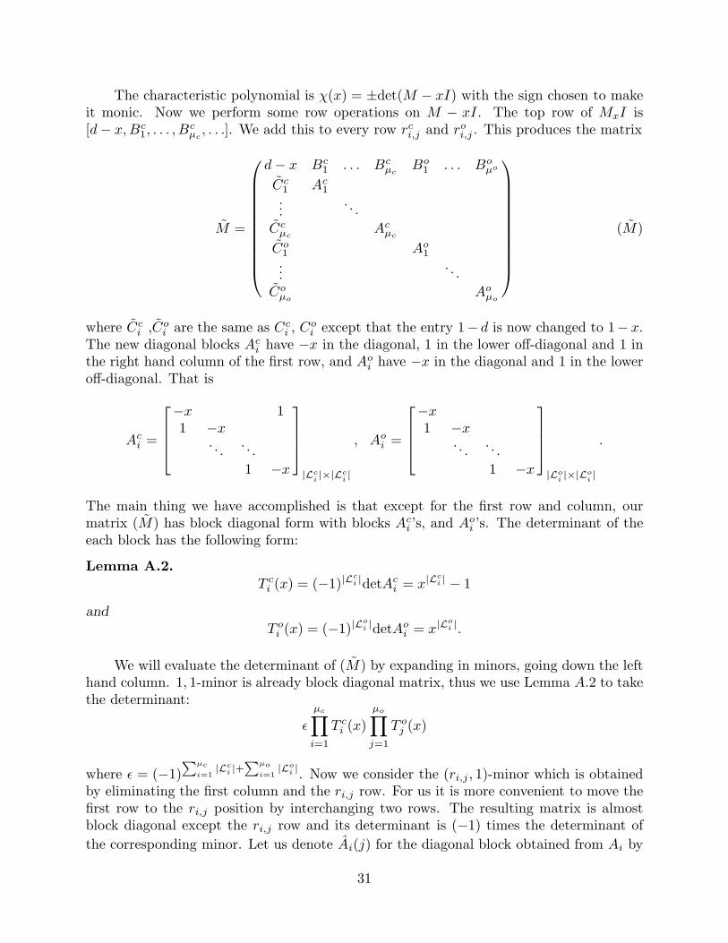
The characteristic polynomial is χ(x) = ±det(M − xI) with the sign chosen to makeit monic. Now we perform some row operations on M − xI. The top row of MxI is[d− x, Bc

1, . . . , Bcµc

, . . .]. We add this to every row rci,j and ro

i,j . This produces the matrix

M =

d− x Bc1 . . . Bc

µcBo

1 . . . Boµo

Cc1 Ac

1...

. . .

Ccµc

Acµc

Co1 Ao

1...

. . .

Coµo

Aoµo

(M)

where Cci ,Co

i are the same as Cci , Co

i except that the entry 1− d is now changed to 1− x.The new diagonal blocks Ac

i have −x in the diagonal, 1 in the lower off-diagonal and 1 inthe right hand column of the first row, and Ao

i have −x in the diagonal and 1 in the loweroff-diagonal. That is

Aci =

−x 11 −x

. . .. . .

1 −x

|Lci|×|Lc

i|

, Aoi =

−x1 −x

. . .. . .

1 −x

|Loi|×|Lo

i|

.

The main thing we have accomplished is that except for the first row and column, ourmatrix (M) has block diagonal form with blocks Ac

i ’s, and Aoi ’s. The determinant of the

each block has the following form:

Lemma A.2.

T ci (x) = (−1)|L

ci |detAc

i = x|Lci | − 1

andT o

i (x) = (−1)|Loi |detAo

i = x|Loi |.

We will evaluate the determinant of (M) by expanding in minors, going down the lefthand column. 1, 1-minor is already block diagonal matrix, thus we use Lemma A.2 to takethe determinant:

ǫ

µc∏

i=1

T ci (x)

µo∏

j=1

T oj (x)

where ǫ = (−1)∑

µc

i=1|Lc

i |+∑

µo

i=1|Lo

i |. Now we consider the (ri,j , 1)-minor which is obtainedby eliminating the first column and the ri,j row. For us it is more convenient to move thefirst row to the ri,j position by interchanging two rows. The resulting matrix is almostblock diagonal except the ri,j row and its determinant is (−1) times the determinant of

the corresponding minor. Let us denote Ai(j) for the diagonal block obtained from Ai by

31

replacing the row ri,j by Bi. For a fixed i, ri,j , 1-minor for all 1 ≤ j ≤ ℓi correspond to

Li. The sum of determinant of Ai(j) for 1 ≤ j ≤ ℓi is following:

Lemma A.3.

Sci (x) = (−1)|L

ci |+1

ℓci∑

j=1

det Aci (j)

and

Soi (x) = (−1)|L

oi |+1

ℓoi∑

j=1

det Aoi (j).

Proof. Let us consider a closed orbit list Lc = N1, . . . , Nℓ. We will compute the deter-minant of Ac(j) by expanding in minors, going to the right the rj row. Notice that the 1’sin rj row, are not on the diagonal. The minor corresponding the k-th 1 on the left handside of the diagonal, i.e. k < j, is xNk+...Nj−1 . The minor corresponding the k-th 1 onthe left hand side of the diagonal, i.e. i ≥ j, is xN1+...Nk−1+Nj+1+...Nℓ . Summing all thesemonomials for all k’s, we have the determinant of Ac

i (j). For the open orbit list, all theminor corresponding the k-th 1 on the left hand side of the diagonal, i.e. k < j, are zerosince the corresponding matrices are lower triangular matrix with zeros on the diagonal.

For the (rci,j , 1)-minor, 1’s in the off-diagonal block would produce zero block on the

diagonal. For the 1’s on the diagonal block will keep other diagonal blocks as diagonalblocks. Thus by Lemma A.2 and Lemma A.3, sum of the determinant of the (rc

i,j, 1)-minorfor j = 1, . . . , ℓi is given by

ǫSci (x)

∏

k 6=i

T ck (x)

µo∏

j=1

T oj (x)

where ǫ = (−1)∑

µc

i=1|Lc

i |+∑

µo

i=1|Lo

i |.

Proof of Theorem A.1. Combining the previous arguments completes the proof.

References

[AABHM] N. Abarenkova, J.-C. Angles d’Auriac, S. Boukraa, S. Hassani, and J.-M. Maillard,Rational dynamical zeta functions for birational transformations, Phys. A 264 (1999),264–293.

[AABM] N. Abarenkova, J.-C. Angles d’Auriac, S. Boukraa, and J.-M. Maillard, Growth-complexity spectrum of some discrete dynamical systems, Physica D 130 (1999), 27–42.

[B] E. Bedford, On the dynamics of birational mappings of the plane, J. Korean Math.Soc. 40 (2003), 373–390.

[BMV] M.P. Bellon, J.-M. Maillard, and C.-M. Viallet, Integrable Coxeter groups, Phys. Lett.A 159 (1991), 221–232.

[BV] M.P. Bellon and C.-M. Viallet, Algebraic entropy, Comm. Math. Phys. 204 (1999),425–437.

32

[BTR] M. Bernardo, T.T. Truong and G. Rollet, The discrete Painleve I equations: tran-scendental integrability and asymptotic solutions, J. Phys. A: Math. Gen., 34 (2001),3215–3252.

[BHM] S. Boukraa, S. Hassani, J.-M. Maillard, Noetherian mappings, Physica D, 185 (2003),no. 1, 3–44.

[BM] S. Boukraa and J.-M. Maillard, Factorization properties of birational mappings, Phys-ica A 220 (1995), 403–470.

[DF] J. Diller and C. Favre, Dynamics of bimeromorphic maps of surfaces, Amer. J. ofMath., 123 (2001), 1135–1169.

[DS] T.-C. Dinh and N. Sibony, Une borne superieure pour l’entropie topologique d’uneapplication rationnelle. arXiv:math.DS/0303271

[FV] G. Falqui and C.-M. Viallet, Singularity, complexity, and quasi-integrability of rationalmappings, Comm. Math. Phys. 154 (1993), 111–125.

[FS] J-E Fornæss and N. Sibony, Complex dynamics in higher dimension: II, Annals ofMath. Stud., vol. 137, Princeton University Press, 1995, pp. 135–182.

[G] V. Guedj, Dynamics of polynomial mappings of C2, Amer. J. of Math., 124 (2002),75–106.

[HP] F.R. Harvey and J. Polking, Extending analytic objects, Comm. Pure Appl. Math.28 (1975), 701–727.

[RGMR] A. Ramani, B. Grammaticos, J.-M. Maillard and G. Rollet, Integrable mappings frommatrix transformations and their singularity properties, J. Phys. A: Math. Gen. 27(1994), 7597–7613.

[R1] K.V. Rerikh, Cremona transformation and general solution of one dynamical systemof the static model, Physica D, 57 (1992), 337–354.

[R2] K.V. Rerikh, Non-algebraic integrability of the Chew-Low reversible dynamical systemof the Cremona type and the relation with the 7th Hilbert problem (non-resonantcase), Physica D, 82 (1995), 60–78.

[R3] K.V. Rerikh, Nonalgebraic integrability of one reversible dynamical system of theCremona type, J. of Math. Physics, 39 (1998), 2821–2832.

[RS] A. Russakovskii and B. Shiffman, Value distribution of sequences of rational mappingsand complex dynamics, Indiana U. Math. J., 46 (1997), 897–932.

[S] N. Sibony, Dynamique des applications rationnelles de Pk, Pano. Synth. 8 (1999),97–185.

[V] C. Viallet, On some rational Coxeter groups, Centre de Recherches Mathematiques,CRM Proceedings and Lecture Notes, Volume 9, 1996, 377–388.

Department of MathematicsIndiana University

Bloomington, IN 47405bedford@indiana.edu

Department of MathematicsSyracuse UniversitySyracuse, NY 13244

kkim26@syr.edu

33