arX

iv:0

904.

1966

v1 [

astr

o-ph

.CO

] 1

3 A

pr 2

009

AJ accepted Apr 07, 2009

On the compact HII galaxy UM 408 as seen by GMOS-IFU:

Physical conditions.

Patricio Lagos1,2

plagos@iac.es

Eduardo Telles1,3

etelles@on.br

Casiana Munoz-Tunon2

cmt@iac.es

Eleazar R. Carrasco4

rcarrasco@gemini.edu

Francois Cuisinier5

francois@ov.ufrj.br

and

Guillermo Tenorio-Tagle6

gtt@inaoep.mx

ABSTRACT

1Observatorio Nacional, Rua Jose Cristino, 77, Rio de Janeiro, 20921-400, Brazil

2Instituto de Astrofisica de Canarias, Via Lactea s/n, 38200 La Laguna, Spain

3Dept. of Astronomy, University of Virginia, P.O.BOX 400325, Charlottesville, VA, 22904-4325, USA

4Gemini Observatory/AURA, Southern Operations Center, Casilla 603, La Serena, Chile

5Observatorio do Valongo UFRJ, Ladeira do Pedro Antonio 43, Rio de Janeiro, 20080-090, Brazil

6Instituto Nacional de Astrofisica Optica y Electronica, AP 51, 72000 Puebla, Mexico

– 2 –

We present Integral Field Unit GMOS-IFU data of the compact HII galaxy

UM 408, obtained at Gemini South telescope, in order to derive the spatial dis-

tribution of emission lines and line ratios, kinematics, plasma parameters, and

oxygen abundances as well the integrated properties over an area of 3′′×4′′.4

equivalent with ∼750 × 1100 pc located in the central part of the galaxy. The

starburst in this area is resolved into two giant regions of about 1′′.5 and 1′′ (∼375

and ∼250 pc) diameter, respectively and separated 1.5-2′′ (∼500 pc). The ex-

tinction distribution concentrate its highest values close but not coincident with

the maxima of Hα emission around each one of the detected regions. This indi-

cates that the dust has been displaced from the exciting clusters by the action of

their stellar winds. The ages of these two regions, estimated using Hβ equivalent

widths, suggest that they are coeval events of ∼5 Myr with stellar masses of

∼104M⊙. We have also used [OIII]/Hβ and [SII]/Hα ratio maps to explore the

excitation mechanisms in this galaxy. Comparing the data points with theoreti-

cal diagnostic models, we found that all of them are consistent with excitation by

photoionization by massive stars. The Hα emission line was used to measure the

radial velocity and velocity dispersion. The heliocentric radial velocity shows an

apparent systemic motion where the east part of the galaxy is blueshifted, while

the west part is redshifted, with a relative motion of ∼ 10 km s−1. The veloc-

ity dispersion map shows supersonic values typical for extragalactic HII regions.

Oxygen abundances were calculated from the [OIII]λλ4959,5007/[OIII]λ4363 ra-

tios. We derived an integrated oxygen abundance of 12+log(O/H)=7.87 summing

over all spaxels in our field of view. An average value of 12+log(O/H)=7.77

and a difference of ∆(O/H)=0.47 between the minimum and maximum values

(7.58±0.06-8.05±0.04) were found, considering all data points where the oxygen

abundance was measured. The spatial distribution of oxygen abundance does

not show any significant gradient across the galaxy. On the other hand, the bulk

of data points are lying in a region of ±2σ dispersion (with σ=0.1 dex) around

the average value, confirming that this compact HII galaxy as other previously

studied dwarf irregular galaxies is chemically homogeneous. Therefore, the new

metals processed and injected by the current star formation episode are possibly

not observed and reside in the hot gas phase, whereas the metals from previous

events are well mixed and homogeneously distributed through the whole extent

of the galaxy.

Subject headings: galaxies: individual (UM 408) — galaxies: abundances —

galaxies: dwarf — galaxies: ISM.

– 3 –

1. Introduction

HII galaxies (or Blue Compact Dwarfs, BCDs) are low-mass and metal-poor galaxies

(1/50-1/3Z⊙), experiencing strong episodes of star formation, characterized by the pres-

ence of bright emission lines on a faint blue continuum (Terlevich et al. 1991; Kehrig et al.

2004). Several studies (e.g, Papaderos et al. 1996; Telles & Terlevich 1997; Cairos et al. 2003;

Westera et al. 2004) have shown the existence of an old stellar population underlying the

present burst in most of these galaxies, indicating that these objects are not young systems

forming their first generation of stars.

The star formation activity in HII galaxies is concentrated in several luminous star

clusters (∼1-30 pc in size) spread over the galaxies. Some of these clusters have been asso-

ciated with super star clusters (SSCs), similar to those found in interacting galaxies, such

as the antennae (Whitmore & Schweizer 1995; Whitmore et al. 1999), and some local dwarf

galaxies such as Henize 2-10 (Conti & Vacca 1994) and NGC 1569 (e.g., O’Connell et al.

1994; Arp & Sandage 1985). During their evolution, these clusters ionize the interstellar

medium (ISM) causing the formation of giant HII regions (GHIIRs), and release a consider-

able quantity of mechanical energy into the ISM, characterized by supersonic motions (e.g,

Melnick et al. 1987), sweeping up the surrounding medium, removing the gas and dust from

the star formation site, while producing structures such as bubbles and supershells. Ulti-

mately, the evolution of these young clusters also causes the freshly produced metals to be

dumped into the ISM.

Oxygen and other α elements are produced by massive stars (>8-10 M⊙) and are re-

leased into the ISM during their supernova phase. These metals will be dispersed in the

whole galaxy and mixed via hydrodynamic mechanisms in time scales of few 108 yrs (e.g.,

Tenorio-Tagle 1996). Since the spatial distribution of abundances of O, N, etc depends on

the recycling time of the ISM, the spatial variation of these abundances give important

insights about these processes. The spatial distribution of emission line ratios and of the

abundance of certain elements in dwarf galaxies have been studied by different authors (e.g.,

Kobulnicky & Skillman 1996, 1997; Lee et al. 2006). In these works the radial and spatial

distribution of the O/H abundance, obtained from the analysis of their H II regions, have

been used as a chemical evolution indicator. Localized nitrogen self enrichment has been

measured in a few cases and attributed to the action of strong winds produced by Wolf-Rayet

(W-R) stars (e.g., Walsh & Roy 1989; Kobulnicky et al. 1997), but no oxygen localized en-

richment systems have been confirmed (Kobulnicky & Skillman 1996). In GHIIRs, where

only one star formation region is present, it is usually assumed that the abundance of the

galaxy and their ISM is well represented by the abundance of this single region, assuming

that the metals are well mixed and distributed across the galaxy.

– 4 –

The details of the structure of HII galaxies are important to understand their ionization

mechanisms, star formation feedback and chemical enrichment. These issues have been ac-

tively addressed in studies of the brightest and nearest systems. The large and heterogeneous

HII galaxy sample (Loose & Thuan 1986; Kunth et al. 1988; Telles et al. 1997) includes a

significant number of far less studied objects at larger distances, with small apparent sizes

and with relatively low surface brightness. Typically, HII galaxies contain one or a few star

formation regions, but Hβ images (Lagos et al. 2007) of some compact objects have revealed

that the central region probably hosts a myriad of unresolved star clusters. The present fa-

cilities, with high spatial resolution and high efficiency instruments on large telescopes (8m),

allow us to study these more distant objects to derive their observed properties and relate

them to the better known nearby galaxies, thus having a handle on the intrinsic properties

of star formation as well as possible evolutionary effects.

In this paper we use integral field spectroscopy with Gemini Multi-object Spectrograph

and the Integral Field Unit (GMOS-IFU) at Gemini South in order to study the spatial

distribution of emission lines, their ratios, extinction, abundances and the kinematic prop-

erties of the gas in the interstellar medium of the compact dwarf galaxy UM 408. UM 408

belongs to a subset sample of rare HII galaxies with low metal abundances (i.e. Z< 1/20

Z⊙) with 12 + log(O/H) = 7.66 (Masegosa et al. 1994; Telles 1995), compact morphology,

and very small effective radius (Reff) of only 2′′.1 from previous morphology and surface

brightness studies (Telles & Terlevich 1997). On other hand, Pustilnik et al. (2002) using

high resolution spectroscopy derived an abundance of 12 + log(O/H) = 7.93 and HI obser-

vations (Salzer et al. 2002) reveal an HI mass of log(MHI)=8.815 M⊙. UM 408 is cataloged

by Salzer (1989) as a Dwarf HII Hot Spot with a redshift of 0.0121 (v=3598 km s−1) with

coordinates RA= 02h 11m 23.s4, DEC= 02o 20′

30′′(J2000) at a distance of ∼ 46 Mpc, and V

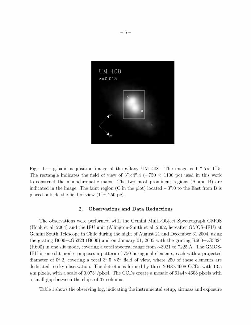
apparent magnitude of 17.38. With the present observations, we note that the central part

of UM 408 encompasses two main star formation regions (here named A and B), as shown

by the g-band acquisition images in Figure 1. Another faint region, called C, can be seen in

the outer parts of the galaxy. These regions were all unresolved in previous studies.

The observations and data reduction procedures are discussed in Section 2. Section 3

gives the results obtained from the 2D emission line maps. In Section 4 we discuss our results

and our conclusions are presented in section 5.

1Value obtained from NED

– 5 –

Fig. 1.— g-band acquisition image of the galaxy UM 408. The image is 11′′.5×11′′.5.

The rectangle indicates the field of view of 3′′×4′′.4 (∼750 × 1100 pc) used in this work

to construct the monochromatic maps. The two most prominent regions (A and B) are

indicated in the image. The faint region (C in the plot) located ∼3′′.0 to the East from B is

placed outside the field of view (1′′≃ 250 pc).

2. Observations and Data Reductions

The observations were performed with the Gemini Multi-Object Spectrograph GMOS

(Hook et al. 2004) and the IFU unit (Allington-Smith et al. 2002, hereafter GMOS–IFU) at

Gemini South Telescope in Chile during the night of August 21 and December 31 2004, using

the grating B600+ G5323 (B600) and on January 01, 2005 with the grating R600+ G5324

(R600) in one slit mode, covering a total spectral range from ∼3021 to 7225 A. The GMOS-

IFU in one slit mode composes a pattern of 750 hexagonal elements, each with a projected

diameter of 0′′.2, covering a total 3′′.5 ×5′′ field of view, where 250 of these elements are

dedicated to sky observation. The detector is formed by three 2048×4608 CCDs with 13.5

µm pixels, with a scale of 0.073′′/pixel. The CCDs create a mosaic of 6144×4608 pixels with

a small gap between the chips of 37 columns.

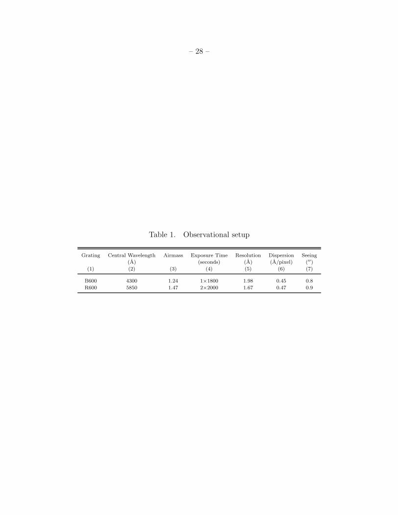
Table 1 shows the observing log, indicating the instrumental setup, airmass and exposure

– 6 –

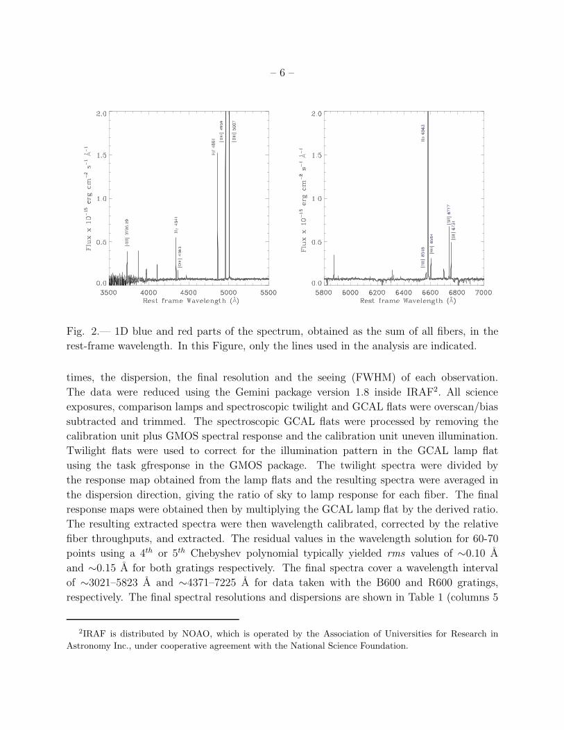
Fig. 2.— 1D blue and red parts of the spectrum, obtained as the sum of all fibers, in the

rest-frame wavelength. In this Figure, only the lines used in the analysis are indicated.

times, the dispersion, the final resolution and the seeing (FWHM) of each observation.

The data were reduced using the Gemini package version 1.8 inside IRAF2. All science

exposures, comparison lamps and spectroscopic twilight and GCAL flats were overscan/bias

subtracted and trimmed. The spectroscopic GCAL flats were processed by removing the

calibration unit plus GMOS spectral response and the calibration unit uneven illumination.

Twilight flats were used to correct for the illumination pattern in the GCAL lamp flat

using the task gfresponse in the GMOS package. The twilight spectra were divided by

the response map obtained from the lamp flats and the resulting spectra were averaged in

the dispersion direction, giving the ratio of sky to lamp response for each fiber. The final

response maps were obtained then by multiplying the GCAL lamp flat by the derived ratio.

The resulting extracted spectra were then wavelength calibrated, corrected by the relative

fiber throughputs, and extracted. The residual values in the wavelength solution for 60-70

points using a 4th or 5th Chebyshev polynomial typically yielded rms values of ∼0.10 A

and ∼0.15 A for both gratings respectively. The final spectra cover a wavelength interval

of ∼3021–5823 A and ∼4371–7225 A for data taken with the B600 and R600 gratings,

respectively. The final spectral resolutions and dispersions are shown in Table 1 (columns 5

2IRAF is distributed by NOAO, which is operated by the Association of Universities for Research in

Astronomy Inc., under cooperative agreement with the National Science Foundation.

– 7 –

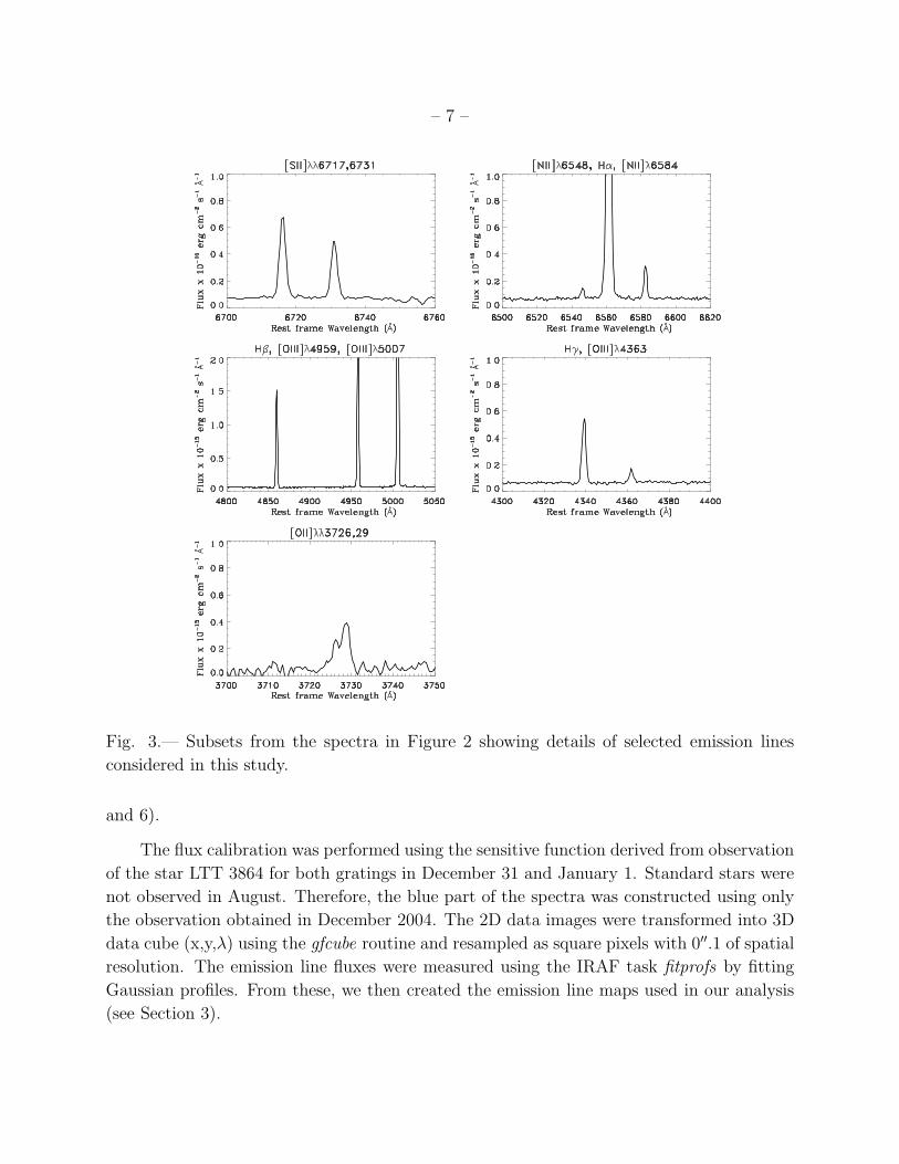
Fig. 3.— Subsets from the spectra in Figure 2 showing details of selected emission lines

considered in this study.

and 6).

The flux calibration was performed using the sensitive function derived from observation

of the star LTT 3864 for both gratings in December 31 and January 1. Standard stars were

not observed in August. Therefore, the blue part of the spectra was constructed using only

the observation obtained in December 2004. The 2D data images were transformed into 3D

data cube (x,y,λ) using the gfcube routine and resampled as square pixels with 0′′.1 of spatial

resolution. The emission line fluxes were measured using the IRAF task fitprofs by fitting

Gaussian profiles. From these, we then created the emission line maps used in our analysis

(see Section 3).

– 8 –

At shorter wavelength the IFU spectroscopy and long-slit observations suffer a spatial

translation produced by differential atmospheric refraction (DAR). This effect is wavelength

dependent, and is produced by the deviation of the light when it passes through the at-

mosphere due to the variation of the air density as a function of elevation. In order to

obtain fluxes corrected of DAR, we used a similar procedure as described in Arribas et al.

(1999) and also applied by Westmoquette et al. (2007a). First we splitted the data cube

in monochromatic images, and for each image we calculated the centroid of an unresolved

point source in the field of view, that in our case corresponds to region A. Finally, the various

monochromatic maps were aligned by shifting the centroids to the same position.

In Figure 2 we show the resultant spectrum for the two gratings used, obtained from the

sum of all GMOS-IFU fibers. Figure 3 shows a detailed view of the selected emission lines

considered in this study. The spectral resolution of the GMOS-IFU observations allow us to

resolve the [OII]λλ3726,29 doublet lines in a limited number of apertures with a ∆λ=2.32 A

between the peak of the lines in the integrated spectrum (see Figure 3). The low intensity of

[OII]λλ3726,29 lines and [OIII]λ4363 are the largest sources of uncertainties in our results.

An automatic procedure to measure these emission line fluxes was not possible, therefore

these lines were measured manually using splot.

3. Results

3.1. Emission line, continuum and EW(Hβ) maps

We used a flux measurement procedure described in the previous section to produce the

maps for the following emission lines: [SII]λ6731, [SII]λ6717, [NII]λ6584, Hα, [OIII]λ5007,

[OIII]λ4959, Hβ, [OIII]λ4363, Hγ, [OII]λλ3726,29, Hα and Hβ continuum and EW(Hβ),

in a rectangular field of 3′′×4′′.4 (see Figure 1). In order to reduce the number of data

points without loosing spatial information and S/N, the data were resampled to 0′′.2 in

spatial resolution. Typical S/N ratios for individual pixels (spaxels in our data cube) for

[OIII]λ5007 are &700 and & 500 for regions A and B, respectively. The [OIII]λ4363 line

shows a typical S/N ratio &8 and &4 for regions A and B, respectively. The signal to noise

for each emission line is given by the ratio between the emission line peak and the RMS of the

adjacent continuum. Figure 4 shows some of the observed emission line maps. All emission

and continuum maps in this Figure are in units of × 10−18 erg cm−2 s−1, except for the Hβ

equivalent width map, which is in units of A. Here 0′′.2 ≈ 50 pc (distances in this work were

computed assuming a Hubble constant of H0=72 km s−1 Mpc−1). Since most of the emission

lines were measured using an automatic procedure, we filtered the maps assigning the value

0 erg cm−2s−1 to all pixels with S/N<3.

– 9 –

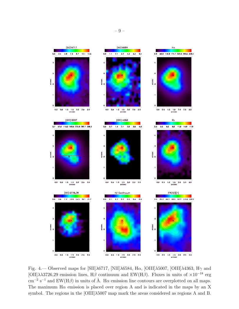
Fig. 4.— Observed maps for [SII]λ6717, [NII]λ6584, Hα, [OIII]λ5007, [OIII]λ4363, Hγ and

[OII]λλ3726,29 emission lines, Hβ continuum and EW(Hβ). Fluxes in units of ×10−18 erg

cm−2 s−1 and EW(Hβ) in units of A. Hα emission line contours are overplotted on all maps.

The maximum Hα emission is placed over region A and is indicated in the maps by an X

symbol. The regions in the [OIII]λ5007 map mark the areas considered as regions A and B.

– 10 –

The maps in Figure 4 show essentially the same spatial distribution, presenting two well

defined and regular regions, that we have labeled A and B. The maximum peak intensity

of the Hα emission line in region A is indicated in the maps by an X symbol. The recom-

bination lines Hα, Hβ and Hγ have very similar spatial distribution to the forbidden lines

in Figure 4, but there is a slight difference in the spatial distribution of [OIII]λ4363 and

[OII]λλ3726,29 over region B. The last two images in Figure 4 corresponds to the spatial

distribution of the Hβ continuum and the EW(Hβ), respectively. It is clear from the maps

that the continuum peak is not coincident with the maximum in Hα emission. This has been

previously reported by other authors (e.g., Sargent & Filippenko 1991; Maiz-Apellaniz et al.

1998; Lagos et al. 2007) in some galaxies with single and multiple star forming regions. In

NGC 4214, Sargent & Filippenko (1991) and Maiz-Apellaniz et al. (1998) found that the

continuum peak emission was displaced in relation to the line emitting regions where a

strong Wolf-Rayet (WR) feature (HeII λ4686 A) was also seen. No WR signatures were

detected in the spectra of UM 408.

The largest EW(Hβ) values in the galaxy are associated with region A, indicating that

this region is younger than region B. On the other hand, the Hβ continuum map (see Figure

4) shows the largest values over region B. In Section 4, the EW(Hβ) values are used as

a proxy for the starburst ages in order to derive the integrated physical properties of the

galaxy and their star forming regions. The error associated to each emission line (σi) was

calculated using the relationship given in Castellanos et al. (2002):

σi = σcN1/2

√

1 +EW

N△, (1)

where σc is the standard deviation in the local continuum associated to each emission line,

N is the number of pixels, EW is the equivalent width of the line and △ is the instrumental

dispersion in A (see Table 1 ). These estimated errors will be used later in the derivation of

uncertainties in the oxygen abundance determination and integrated properties.

Finally, given that the seeing was 0.8-0.9′′ (∼4 pixels in the emission line maps), each

aperture or pixel of 0.2′′ should be correlated with its neighbor, and the pixel-to-pixel varia-

tions in the maps produced from the observed emission line are likely due to the uncertainties

attached to the measurement and do not represent real variations. Therefore, we smoothed

the emission line ratio, temperature and oxygen abundance maps using a 3×3 box.

– 11 –

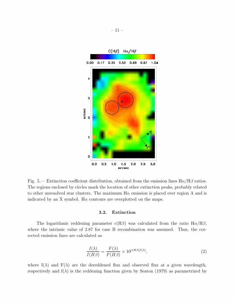
Fig. 5.— Extinction coefficient distribution, obtained from the emission lines Hα/Hβ ratios.

The regions enclosed by circles mark the location of other extinction peaks, probably related

to other unresolved star clusters. The maximum Hα emission is placed over region A and is

indicated by an X symbol. Hα contours are overplotted on the maps.

3.2. Extinction

The logarithmic reddening parameter c(Hβ) was calculated from the ratio Hα/Hβ,

where the intrinsic value of 2.87 for case B recombination was assumed. Thus, the cor-

rected emission lines are calculated as

I(λ)

I(Hβ)=

F (λ)

F (Hβ)× 10c(Hβ)f(λ), (2)

where I(λ) and F(λ) are the dereddened flux and observed flux at a given wavelength,

respectively and f(λ) is the reddening function given by Seaton (1979) as parametrized by

– 12 –

Howarth (1983), using appropriated values for the Milky Way (Kobulnicky et al. 1997).

Figure 5 shows the smoothed spatial distribution of c(Hβ) for the emission line ratios

mentioned above. The reddening parameters c(Hβ) were set to 0.0 for unrealistic values of

Hα/Hβ < 2.87. We observe a range of extinction of ∼0.02 to 1.04 with average c(Hβ) value

of 0.76 and a standard deviation of 0.17. The lowest extinction values are located in the outer

part of the field of view (see Figure 5). We note also that the maximum extinction c(Hβ) is

close to, but not coincident with the peak of Hα emission. A similar result has been reported

by Maiz-Apellaniz et al. (1998) and Cairos et al. (2002) for the star formation knots in the

galaxies NGC 4214 and Mrk 370, respectively. Apparently, the current starburst episode in

this galaxy is sweeping the gas and dust out of the center into the surrounding regions. The

emission line distribution as well as the c(Hβ) distribution over region A and its elongated

shape suggest that this region may contain two or more star forming complexes instead of

only one. These complexes are indicated with circles in the extinction maps.

Finally, as the extinction across the galaxy does not show a uniform distribution, con-

centrating the highest values around the star forming regions, the fluxes of each pixel in the

emission line maps were corrected using their corresponding c(Hβ) value.

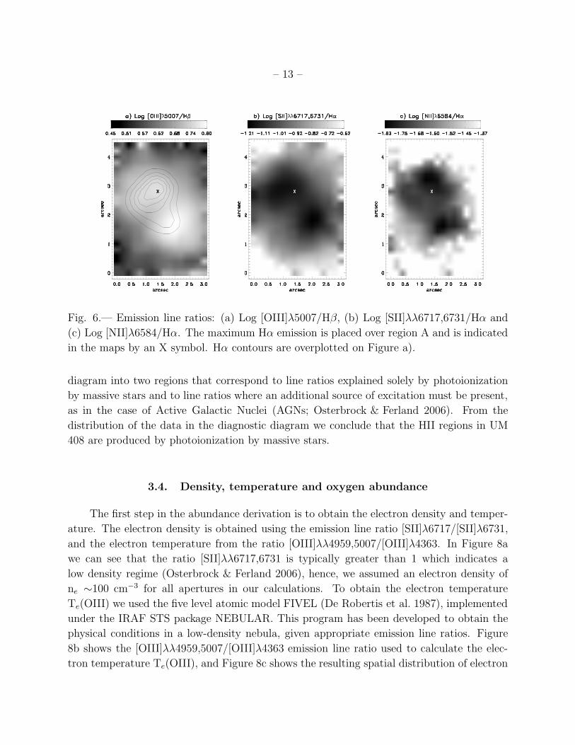
3.3. Nebular emission line diagnostic diagrams

The standard BPT diagnostic diagrams (Baldwin et al. 1981) have been used to ana-

lyze the possible excitation mechanisms present in UM 408. Figure 6 (a, b and c) shows

the following emission line ratio maps: [OIII]λ5007/Hβ ([OIII]/Hβ), [SII]λλ6717,6731/Hα

([SII]/Hα) and [NII]λ6584/Hα ([NII]/Hα). Figure 6 shows that [OIII]/Hβ and [SII]/Hα

ratios have essentially the same spatial distribution with inverse trends. The largest values

of [OIII]/Hβ and the lowest values of [SII]/Hα are seen in the east part of the galaxy, near

region B. The emission line ratios measured within these regions are common to high exci-

tation HII regions with values ranging from log([OIII]/Hβ)=0.45 to 0.80 (all map), 0.65 to

0.76 (region A) and 0.72 to 0.80 (region B), and from log([SII]/Hα)=-1.21 to -0.62 (all map),

-1.17 to -0.85 (region A) and -1.21 to -1.01 (region B). Additionally, the low ionization ratios

[NII]/Hα and [SII]/Hα increase from the center outwards.

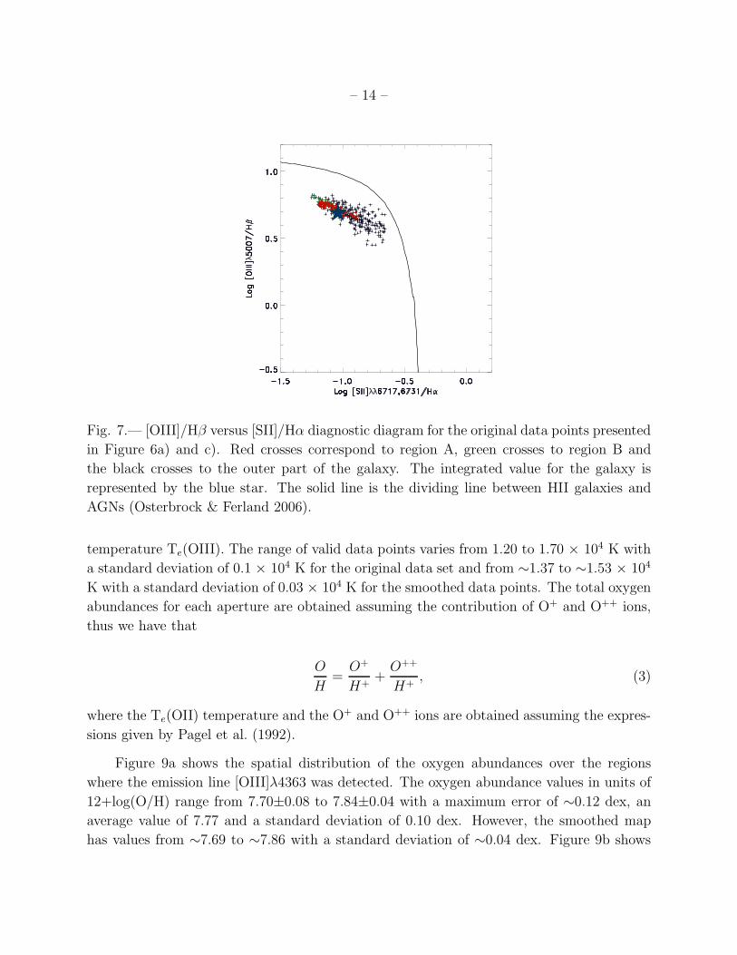
Figure 7 shows the log[OIII]/Hβ vs. log[SII]/Hα diagnostic diagram, identifying three

different regions in UM 408 using the original data points (non-smoothed). Red and green

crosses correspond to regions A and B, respectively, and the black crosses correspond to the

outer parts of the galaxy. The integrated value that represents the sum over all spaxels in

our field of view is given by the blue star symbol. The solid line in Figure 7 divides the

– 13 –

Fig. 6.— Emission line ratios: (a) Log [OIII]λ5007/Hβ, (b) Log [SII]λλ6717,6731/Hα and

(c) Log [NII]λ6584/Hα. The maximum Hα emission is placed over region A and is indicated

in the maps by an X symbol. Hα contours are overplotted on Figure a).

diagram into two regions that correspond to line ratios explained solely by photoionization

by massive stars and to line ratios where an additional source of excitation must be present,

as in the case of Active Galactic Nuclei (AGNs; Osterbrock & Ferland 2006). From the

distribution of the data in the diagnostic diagram we conclude that the HII regions in UM

408 are produced by photoionization by massive stars.

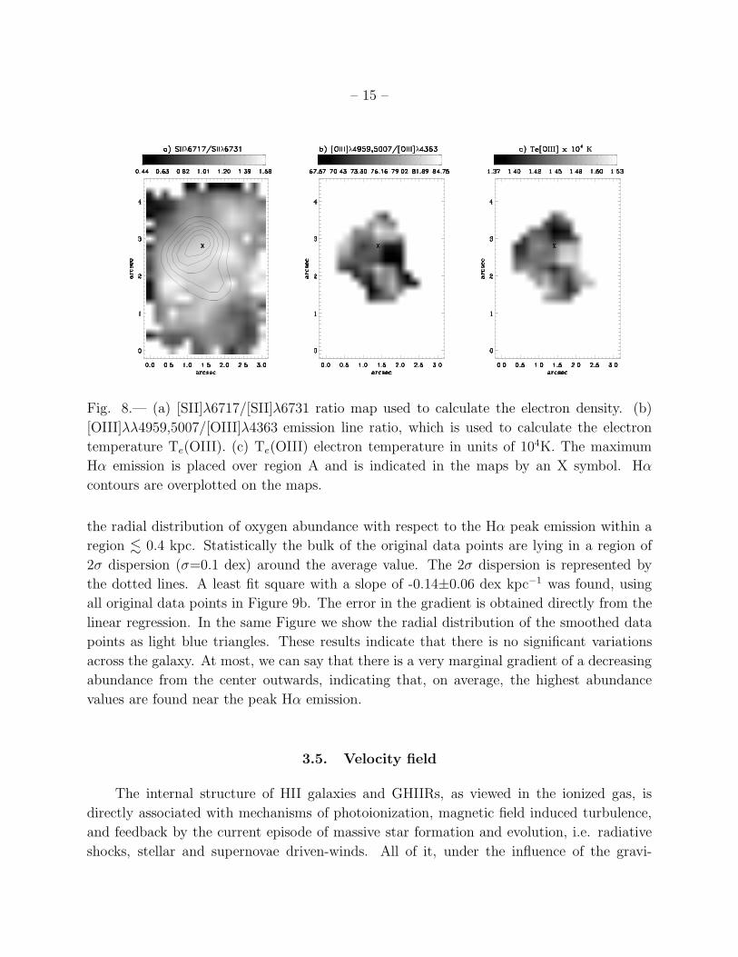
3.4. Density, temperature and oxygen abundance

The first step in the abundance derivation is to obtain the electron density and temper-

ature. The electron density is obtained using the emission line ratio [SII]λ6717/[SII]λ6731,

and the electron temperature from the ratio [OIII]λλ4959,5007/[OIII]λ4363. In Figure 8a

we can see that the ratio [SII]λλ6717,6731 is typically greater than 1 which indicates a

low density regime (Osterbrock & Ferland 2006), hence, we assumed an electron density of

ne ∼100 cm−3 for all apertures in our calculations. To obtain the electron temperature

Te(OIII) we used the five level atomic model FIVEL (De Robertis et al. 1987), implemented

under the IRAF STS package NEBULAR. This program has been developed to obtain the

physical conditions in a low-density nebula, given appropriate emission line ratios. Figure

8b shows the [OIII]λλ4959,5007/[OIII]λ4363 emission line ratio used to calculate the elec-

tron temperature Te(OIII), and Figure 8c shows the resulting spatial distribution of electron

– 14 –

Fig. 7.— [OIII]/Hβ versus [SII]/Hα diagnostic diagram for the original data points presented

in Figure 6a) and c). Red crosses correspond to region A, green crosses to region B and

the black crosses to the outer part of the galaxy. The integrated value for the galaxy is

represented by the blue star. The solid line is the dividing line between HII galaxies and

AGNs (Osterbrock & Ferland 2006).

temperature Te(OIII). The range of valid data points varies from 1.20 to 1.70 × 104 K with

a standard deviation of 0.1 × 104 K for the original data set and from ∼1.37 to ∼1.53 × 104

K with a standard deviation of 0.03 × 104 K for the smoothed data points. The total oxygen

abundances for each aperture are obtained assuming the contribution of O+ and O++ ions,

thus we have that

O

H=

O+

H++

O++

H+, (3)

where the Te(OII) temperature and the O+ and O++ ions are obtained assuming the expres-

sions given by Pagel et al. (1992).

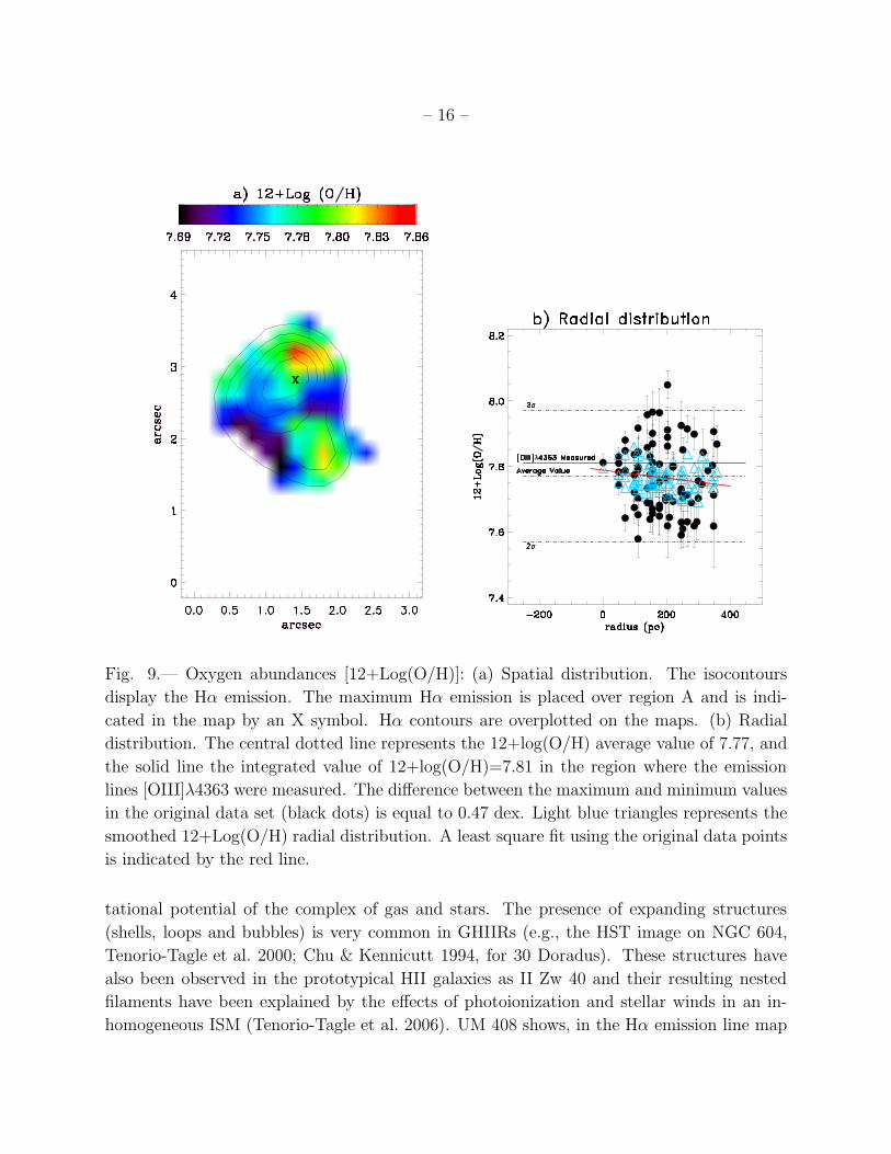
Figure 9a shows the spatial distribution of the oxygen abundances over the regions

where the emission line [OIII]λ4363 was detected. The oxygen abundance values in units of

12+log(O/H) range from 7.70±0.08 to 7.84±0.04 with a maximum error of ∼0.12 dex, an

average value of 7.77 and a standard deviation of 0.10 dex. However, the smoothed map

has values from ∼7.69 to ∼7.86 with a standard deviation of ∼0.04 dex. Figure 9b shows

– 15 –

Fig. 8.— (a) [SII]λ6717/[SII]λ6731 ratio map used to calculate the electron density. (b)

[OIII]λλ4959,5007/[OIII]λ4363 emission line ratio, which is used to calculate the electron

temperature Te(OIII). (c) Te(OIII) electron temperature in units of 104K. The maximum

Hα emission is placed over region A and is indicated in the maps by an X symbol. Hα

contours are overplotted on the maps.

the radial distribution of oxygen abundance with respect to the Hα peak emission within a

region . 0.4 kpc. Statistically the bulk of the original data points are lying in a region of

2σ dispersion (σ=0.1 dex) around the average value. The 2σ dispersion is represented by

the dotted lines. A least fit square with a slope of -0.14±0.06 dex kpc−1 was found, using

all original data points in Figure 9b. The error in the gradient is obtained directly from the

linear regression. In the same Figure we show the radial distribution of the smoothed data

points as light blue triangles. These results indicate that there is no significant variations

across the galaxy. At most, we can say that there is a very marginal gradient of a decreasing

abundance from the center outwards, indicating that, on average, the highest abundance

values are found near the peak Hα emission.

3.5. Velocity field

The internal structure of HII galaxies and GHIIRs, as viewed in the ionized gas, is

directly associated with mechanisms of photoionization, magnetic field induced turbulence,

and feedback by the current episode of massive star formation and evolution, i.e. radiative

shocks, stellar and supernovae driven-winds. All of it, under the influence of the gravi-

– 16 –

Fig. 9.— Oxygen abundances [12+Log(O/H)]: (a) Spatial distribution. The isocontours

display the Hα emission. The maximum Hα emission is placed over region A and is indi-

cated in the map by an X symbol. Hα contours are overplotted on the maps. (b) Radial

distribution. The central dotted line represents the 12+log(O/H) average value of 7.77, and

the solid line the integrated value of 12+log(O/H)=7.81 in the region where the emission

lines [OIII]λ4363 were measured. The difference between the maximum and minimum values

in the original data set (black dots) is equal to 0.47 dex. Light blue triangles represents the

smoothed 12+Log(O/H) radial distribution. A least square fit using the original data points

is indicated by the red line.

tational potential of the complex of gas and stars. The presence of expanding structures

(shells, loops and bubbles) is very common in GHIIRs (e.g., the HST image on NGC 604,

Tenorio-Tagle et al. 2000; Chu & Kennicutt 1994, for 30 Doradus). These structures have

also been observed in the prototypical HII galaxies as II Zw 40 and their resulting nested

filaments have been explained by the effects of photoionization and stellar winds in an in-

homogeneous ISM (Tenorio-Tagle et al. 2006). UM 408 shows, in the Hα emission line map

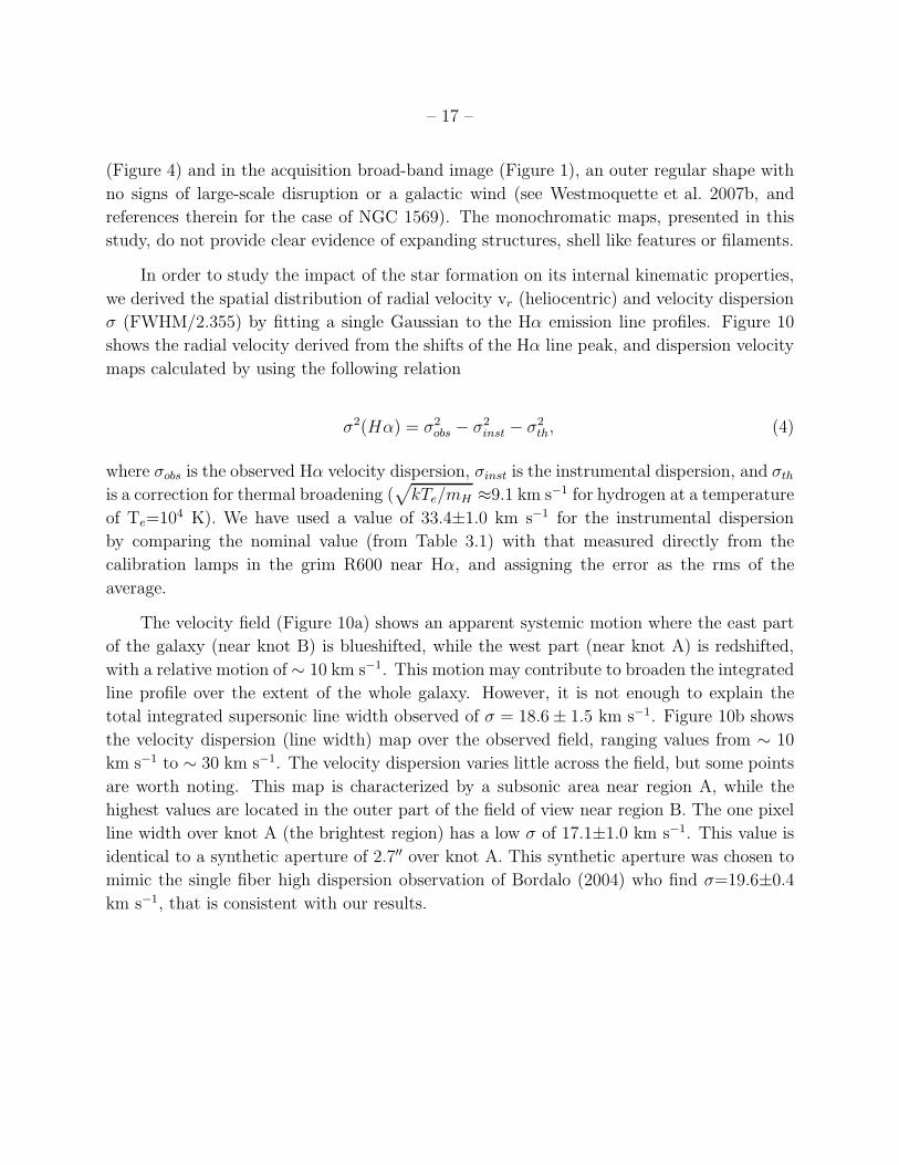
– 17 –

(Figure 4) and in the acquisition broad-band image (Figure 1), an outer regular shape with

no signs of large-scale disruption or a galactic wind (see Westmoquette et al. 2007b, and

references therein for the case of NGC 1569). The monochromatic maps, presented in this

study, do not provide clear evidence of expanding structures, shell like features or filaments.

In order to study the impact of the star formation on its internal kinematic properties,

we derived the spatial distribution of radial velocity vr (heliocentric) and velocity dispersion

σ (FWHM/2.355) by fitting a single Gaussian to the Hα emission line profiles. Figure 10

shows the radial velocity derived from the shifts of the Hα line peak, and dispersion velocity

maps calculated by using the following relation

σ2(Hα) = σ2obs − σ2

inst − σ2th, (4)

where σobs is the observed Hα velocity dispersion, σinst is the instrumental dispersion, and σth

is a correction for thermal broadening (√

kTe/mH ≈9.1 km s−1 for hydrogen at a temperature

of Te=104 K). We have used a value of 33.4±1.0 km s−1 for the instrumental dispersion

by comparing the nominal value (from Table 3.1) with that measured directly from the

calibration lamps in the grim R600 near Hα, and assigning the error as the rms of the

average.

The velocity field (Figure 10a) shows an apparent systemic motion where the east part

of the galaxy (near knot B) is blueshifted, while the west part (near knot A) is redshifted,

with a relative motion of ∼ 10 km s−1. This motion may contribute to broaden the integrated

line profile over the extent of the whole galaxy. However, it is not enough to explain the

total integrated supersonic line width observed of σ = 18.6 ± 1.5 km s−1. Figure 10b shows

the velocity dispersion (line width) map over the observed field, ranging values from ∼ 10

km s−1 to ∼ 30 km s−1. The velocity dispersion varies little across the field, but some points

are worth noting. This map is characterized by a subsonic area near region A, while the

highest values are located in the outer part of the field of view near region B. The one pixel

line width over knot A (the brightest region) has a low σ of 17.1±1.0 km s−1. This value is

identical to a synthetic aperture of 2.7′′ over knot A. This synthetic aperture was chosen to

mimic the single fiber high dispersion observation of Bordalo (2004) who find σ=19.6±0.4

km s−1, that is consistent with our results.

– 18 –

Fig. 10.— (a) Hα radial velocity in units of km s−1. (b) Hα Velocity dispersion σ. The

value showed in this figure is obtained considering an instrumental σinst and thermal σth

correction over the observed value σobs. The maximum Hα emission is placed over region A

and is indicated in the maps by an X symbol.

4. Discussion

4.1. The integrated properties of UM 408

We have measured the flux in two different apertures enclosing more than ∼60% of the

observed Hα flux of the galaxy in order to study the properties of the star formation regions

detected in this galaxy. One aperture for region A (48% of the measured Hα flux) and another

for region B (13% of the measured Hα flux). These regions have a diameters of about 1′′.5

and 1′′ that correspond to approximately 375 pc and 250 pc, respectively. Regions A and B

are indicated in the [OIII]λ5007 map of Figure 4. These regions are formed by the data points

where the [OIII]λ4363 emission line is detected. To obtain the integrated properties of the

galaxy and compare with previous observations (e.g. Masegosa et al. 1994; Pustilnik et al.

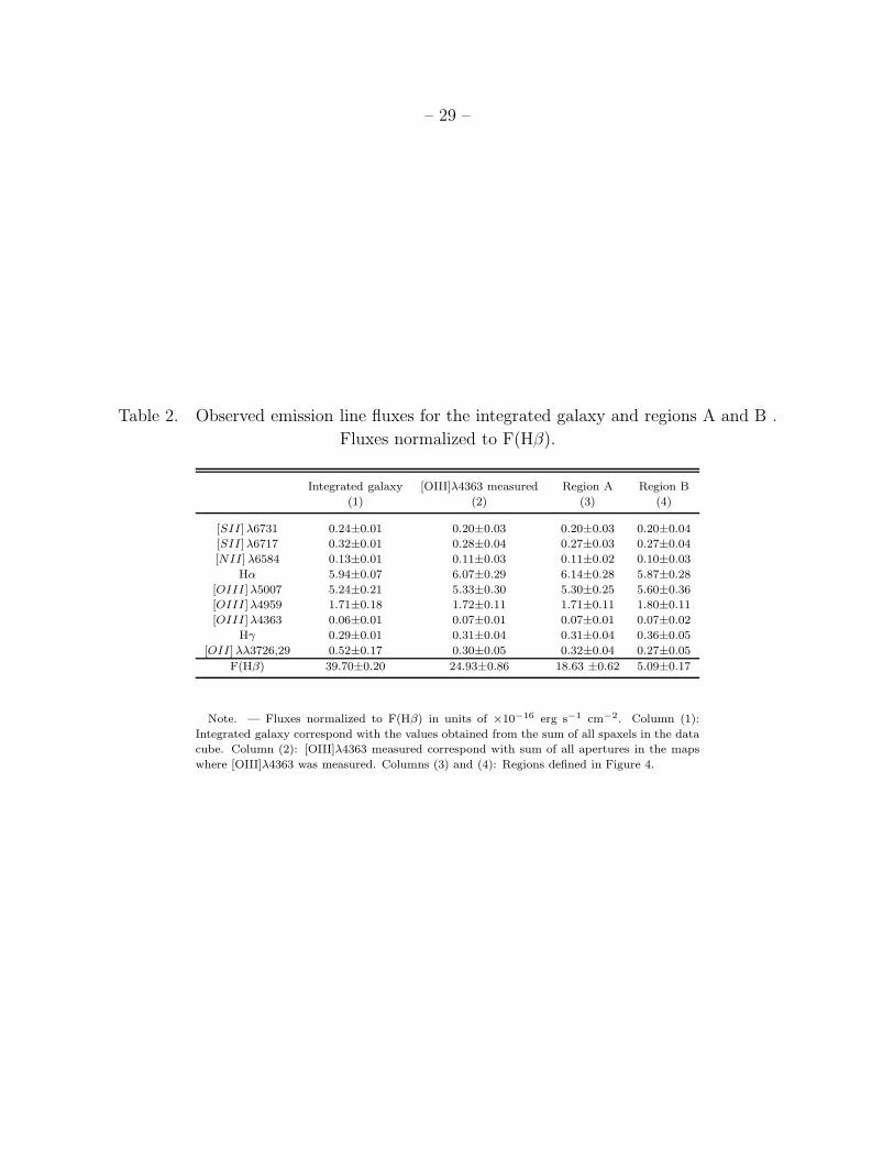
2002) we derived the integrated spectra summing over all pixels in our data cube. Table 2

– 19 –

summarizes the resultant emission line values, obtained using the different synthetic aper-

tures, including the total [OIII]λ4363 aperture over the galaxy (in regions where [OIII]λ4363

emission line is detected and measured). These measurements are in reasonable agreement

with those derived with long slit spectroscopy (e.g., Terlevich et al. 1991; Masegosa et al.

1994; Pustilnik et al. 2002) considering aperture differences and observational uncertainties.

A larger discrepancy however occurs between our observed [OII]λλ3726,29/Hβ value of 0.52

and that of Pustilnik et al. (2002) of 1.45. However, their value must be overestimated since,

from their Figure 1, we clearly see that Hβ > [OII]λ3727.

The observed EW(Hβ) values in UM 408 are ∼102 A and ∼57 A for regions A and B

and ∼67 A for the integrated galaxy, respectively. The values for regions A and B have been

calculated by taking the average over all pixels in each region. Using these EW(Hβ) values we

can estimate the cluster ages by comparison with the values obtained from STARBURST99

model (Leitherer et al. 1999). The resulting ages assuming an instantaneous burst and a

metallicity of Z=0.004 for a Salpeter IMF with a mass limit of 1M⊙ to 100M⊙ are 4.83 Myrs

and 5.00 Myrs for regions A and B, respectively. These ages are consistent with both regions

being formed simultaneously. We found integrated luminosities (assuming a distance of

D=46.8 Mpc; Pustilnik et al. 2002) of Log L(Hα)=39.15, 38.58 and 39.47 erg s−1 for regions

A and B and for the integrated galaxy, respectively. These correspond to a star formation

rate of SFR=0.011, 0.003 and 0.024 M⊙ yr−1, and with a number of ionizing photons log

Q(H0)=51.01, 50.45 and 51.34 photons s−1 for regions A, B and for the integrated galaxy,

obtained from the relationships given by Kennicutt (1998). The masses of these regions can

be estimated by scaling the number of ionizing photons with the models predicted for the

corresponding ages. The stellar masses are 5.17 × 104 M⊙ and 2.29 × 104 M⊙ for regions

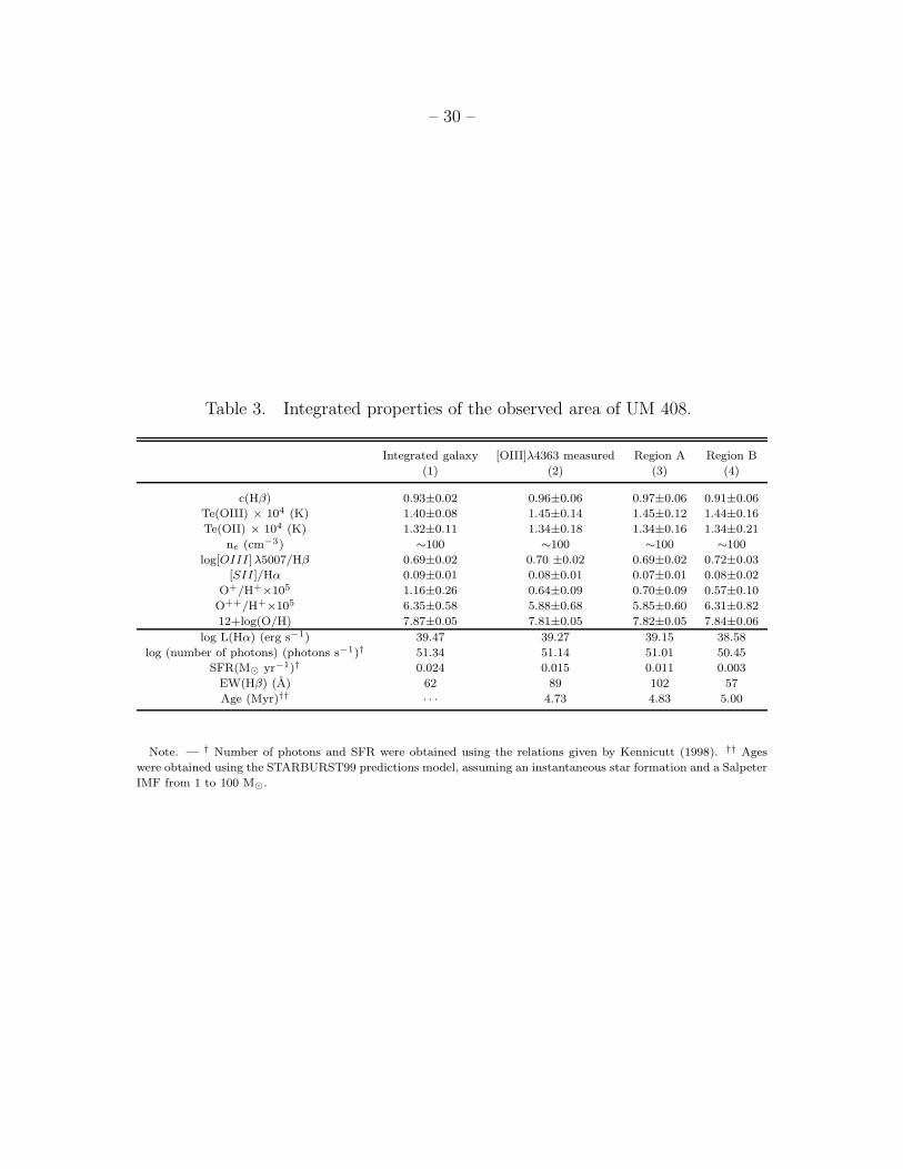
A and B, respectively. Table 3 shows the derived integrated properties of the galaxy and its

star forming regions.

Since its discovery, UM 408 was classified as a low abundance galaxy with an integrated

value of 12+Log(O/H)=7.63 for low resolution spectroscopy (Masegosa et al. 1994) and 7.93

for high resolution spectroscopy (Pustilnik et al. 2002). In this work, we found an integrated

abundance (summing over all spaxels in our field of view) of 12+Log(O/H)=7.87±0.05.

The synthetic apertures previously mentioned, yield an integrated oxygen abundance of

12+Log(O/H)=7.82±0.05 and 7.84±0.06 for regions A and B, respectively. Measuring the

abundance in an aperture equivalent with the area where the emission line [OIII]λ4363 was

measured we obtain a value of 7.81±0.05, the same value obtained in the peak of the Hα

emission (see Figure 9b). This result reflects the fact that the integrated values are light

weighted and dominated by the galaxy peak emission.

Finally, despite the fact that a detailed kinematic analysis is beyond the scope of the

– 20 –

present paper, our results confirm that the core dominates the kinematic information of the

star forming region, and present a low σ value, as found by other works (e.g., Telles et al.

2001, and references therein). Therefore, a single Gaussian fit to the line profile of any

aperture encompassing the brightest knot will measure a representative line width of the

dominant supersonic motions, somewhat deconvolved by the effects of stellar and SN me-

chanical energy input. The effects of stellar or SN feedback will contribute to the broadening

of the line profiles, but will only be detectable in the lower density regions at low intensi-

ties. One means to recognize these effects is through the identification of inclined bands in

the diagnostic diagrams of intensity vs. σ as proposed by Munoz-Tunon et al. (1996) and

Yang et al. (1996). However, the compactness of UM 408 and the small range of reliable

line widths make the use of the diagnostic diagrams difficult to interpret in this case. The

Hα line profile is symmetric and well represented by a single Gaussian, and does not show

prominent low intensity wings in either apertures. An attempt to deblend a possible addi-

tional component to this line profile produced only an upper limit of σbroad ≤ 100 km s−1

with F (α)broad/F (α)narrow ≤ 3%.

4.2. Distribution of the oxygen abundance and their comparison with other

dwarf galaxies

The uniform behavior of O/H abundance in scales of hundreds of pc in low mass galaxies

as in UM 408 is not without precedent, and is comparable with the observed variation in

some dwarf galaxies by other authors. In NGC 4214 (Dwarf Irregular/Wolf-Rayet galaxy)

Kobulnicky & Skillman (1996) showed that there is no localized O, N or He abundance

gradients, but they found, near the youngest region, an oxygen overabundance of 0.095±0.019

dex. Kobulnicky & Skillman (1997), using long slit spectroscopy to study the interstellar

medium of the dwarf irregular galaxy NGC 1569, failed to find evidence for O/H gradient

from the recent star formation activity. Lee et al. (2006) studied the local group dwarf

irregular galaxy NGC 6822 and measured a difference of ∆(O/H)=0.53 dex between the

maximum (8.43±0.2) and minimum value (7.90±0.1), with a mean oxygen abundance of

12+log(O/H)=8.11±0.1 using only the HII regions where the [OIII]λ4363 emission lines

were detected. A gradient of -0.14±0.07 dex kpc−1 was measured by Lee et al. in a radius

.1.4 kpc, and a slope of -0.16 dex kpc−1 was obtained if measurements from the literature

were included, showing the existence of a possible radial gradient in oxygen abundance.

Izotov et al. (2006) using VLT/GIRAFFE in the ARGUS mode, observed the dwarf galaxy

SBS 0335-052E, one of the most metal poor galaxies with an integrated oxygen abundance of

12+log(O/H)=7.30 (Melnick et al. 1992). The spatial distribution of the oxygen abundance

in the ISM of SBS 0335-052E vary from 7.00±0.08 to 7.42±0.02, representing a difference

– 21 –

of ∆(O/H)=0.42 dex. The maximum value of oxygen abundances in this galaxy does not

correspond to the position of one of the identified SSCs, but Izotov et al. find a slight trend

of a decreasing abundance, interpreted as possible self-enrichment. However, they argue that

the errors in the calculated oxygen abundances and Te, ne, etc, not considering instrumental

and observational uncertainties, lead to consider the oxygen abundance variations in SBS

0335-052E may not be statistically significant. More recently, using IFU-PMAS observations,

Kehrig et al. (2008) studied the spatial distribution of some metals over the galaxy IIZw70.

In this study they find a difference of △(O/H)=0.40 dex between the maximum (8.05±0.06)

and minimum (7.65±0.06) values of oxygen abundance. In the case of UM 408, the bulk of

our observed data points are distributed in a region of ±2σ dispersion around the average

value with a difference between the maximum and minimum values of 0.47 dex. This is,

somewhat, in good agreement with previous results in other dwarf galaxies, using in some

cases different techniques. We note that the gradient found in our work, calculated in a

spatial scale of hundreds of pc, is similar to the gradients calculated in other studies in scales

of kpc. Finally, the two giant regions A and B show a difference of oxygen abundance of

only △(O/H)=0.02 dex, which indicates that these regions show identical chemical properties

within the errors. Given the ages (∼5 Myr) and stellar masses (∼104M⊙) of these regions,

we expect that hundreds of SNs have exploded, producing eventually localized enrichments.

But the absence of chemical overabundances in the ISM of UM 408 and in the dwarf galaxies

studied in the literature lead to conclude that the population of young clusters have not

produce preferentially localized overabundances.

These results are compatible with the interpretation that the newly synthesized metals

from the current star formation episode may not be in the warm phase of the ISM, and thus

are not observed at optical wavelengths. The metals that are observed, however, ought to

be from previous events, and may be well mixed and homogeneously distributed over the

whole extent of this low mass and compact galaxy. Note that in UM 408, there is no bar

induced rotation, or shear, to produce the metal dispersal and mixing as in more massive

galaxies (e.g., Roy & Kunth 1995), and thus there must be another mechanism responsible

for the large-scale dispersal and mixing with the ISM. One such hydrodynamic mechanism

for the transport and mixing of the metals produced by compact bursts of star formation

into the ISM has been proposed by Tenorio-Tagle (1996). This model predicts that the

energy injected by core-collapse supernovae change the physical conditions (density and

temperature) of the interstellar medium, while undergoing a long excursion into the galactic

volume. The injected matter is first thermalized, near the starburst, as it goes through a

reverse shock. This generates the giant pressure that allows for the built up of superbubbles,

kpc scale structures that may grow for up to 50 Myr. Afterwards, once the SN II phase is

over, the giant superbubble gas begins to cool down by radiation. This happens first within

– 22 –

the parcels of gas that present the largest densities, promoting their thermal instability.

The sudden loss of pressure within densest parcels of gas would immediately trigger the

appearance of re-pressurizing shocks emanating from the low density hot gas. The process

leads to a plethora of dense condensations that inevitably will fall and settle within the main

body of the galaxy. The process of cooling and dispersal onto the main body of the galaxy

will occur within a few 108 yr. For a complete mixing, the model assumes that a further star

formation episode has to occur and through photoionization the metal enrich condensations

will expand and be fully mixed with the ISM (see also Stasinska et al. 2007). This scenario

seems plausible and compatible with our analysis for the case of UM 408.

5. Conclusions

We used GMOS-IFU spectrum of the compact HII galaxy UM 408, in order to derive

the spatial distribution of emission line ratios, extinction c(Hβ), radial velocity vr, velocity

dispersion σ, electron temperature and oxygen abundance (O/H) as well the integrated

properties over an extended region of 3′′×4′′.4 equivalent to 750 × 1100 pc in the central

part of the galaxy. Below, we summarize our results and conclusions.

1. The observed region of the galaxy includes two giant HII regions not resolved in pre-

vious studied, here labelled A and B. The sizes of these ionized regions are ∼375 and

∼250 pc for regions A and B, respectively. Another region labelled C was found to the

East of region B. We do not observe large scale structures as in other GHIIRs and HII

galaxies in the monochromatic maps.

2. The distribution of dust content in the galaxy was derived from the Balmer line decre-

ment (Hα/Hβ). The c(Hβ) distribution concentrates the highest values close but not

coincident with the peak of Hα emission in each ionized cluster (A and B). The dust

seems to be displaced from the star formation regions by the action of the star cluster

winds.

3. We used [OIII]/Hβ and [SII]/Hα ratios to investigate the possible excitation mechanism

over the ISM of the galaxy. Comparing the data points in the diagnostic diagram

with the theoretical model given by Osterbrock & Ferland (2006), we found that all

measured Hα flux arises from gas photoionized by massive stars

4. The velocity field (vr) shows an apparent systemic motion where the east part of the

galaxy (near knot B) is blueshifted, while the west part (near knot A) is redshifted, with

a relative motion of ∼ 10 km s−1 and a difference between the maximum a minimum

– 23 –

values of ∼33 km s−1. The velocity dispersion map shows supersonic values, typical

for extragalactic HII regions, ranging values from ∼ 10 km s−1 to ∼ 30 km s−1.

5. The ages of the two giant regions detected in this study, were estimated from their

EW(Hβ) and the STARBURST99 models, suggesting that they are coeval events of

∼5 Myr with stellar masses of ∼104 M⊙. We see a marginal difference in the integrated

oxygen abundance between these regions of △(O/H)=0.02 dex.

6. Finally, as found in other nearby dwarf galaxies, we do not observe a gradient in oxygen

abundance across the compact galaxy UM 408. The bulk of the observed data points

are lying in a region of ±2σ dispersion (σ=0.1 dex); therefore, the new metals formed

in the current star formation episodes are not observed and reside probably in the hot

gas phase (T∼107 K), whereas the metals from previous star formation events are well

mixed and homogeneously distributed through the whole extent of the galaxy.

All results presented here are suggestive that UM 408 is an unevolved low metallicity

dwarf galaxy, undergoing a simultaneous episode of star formation over the whole optically

observed extension, and it is a genuine example of the simplest starbursts occurring in

galactic scale, possibly mimicking the properties one expects for young galaxies at high

redshift.

6. Acknowledgments

We would like to thank the anonymous referee for his/her comments and suggestions

which substantially improved the paper. PL acknowledges support from Faperj, Brazil for

his studentship and IAC Spain where part of this work was done. This work has been

partly funded by ESTALLIDOS (see http://www.iac.es/project/GEFE/estallidos) project

AYA2007-67965-C03-01. ET acknowledges his US Gemini Fellowship by AURA, and GTT

acknowledges a research grant 60333 from CONACYT Mexico. Based on observations ob-

tained at the Gemini Observatory, which is operated by the Association of Universities for

Research in Astronomy, Inc., under a cooperative agreement with the NSF on behalf of

the Gemini partnership: the National Science Foundation (United States), the Science and

Technology Facilities Council (United Kingdom), the National Research Council (Canada),

CONICYT (Chile), the Australian Research Council (Australia), Ministerio da Ciencia e Tec-

nologia (Brazil) and Ministerio de Ciencia, Tecnologıa e Innovacion Productiva (Argentina);

Gemini program ID: GS-2004B-Q-59. This research has made use of the NASA/IPAC Ex-

tragalactic Database (NED) which is operated by the Jet Propulsion laboratory, California

– 24 –

Institute of technology, under contract with the National Aeronautics and Space Adminis-

tration.

REFERENCES

Allington-Smith, J., Graham, M., Content, R., Dodsworth, G., Davies, R., Miller, B. W.,

Jørgensen, I., Hook, I., Crampton, D., & Murowinski, R. 2002, PASP, 114, 892

Arp, H., & Sandage, A. 1985, AJ, 90, 1163

Arribas, S., Mediavilla, E., Garcia-Lorenzo, B., del Burgo, C., & Fuensalida, J. J. 1999,

A&AS, 136, 189

Baldwin J.A., Phillips M.M., & Terlevich R. 1981, PASP, 93, 5

Bordalo Vinicius 2004, Tese de Mestrado Observatorio Nacional, Brazil

Cairos, L. M., Caon, N., Garcıa-Lorenzo, B., Vılchez, J. M., & Munoz-Tunon, C. 2002, ApJ,

577, 164

Cairos, L. M., Caon, N., Papaderos, P., Noeske, K., Vılchez, J. M., Lorenzo, B. G., &

Munoz-Tunon, C. 2003, ApJ, 593, 312

Castellanos, M., Dıaz, A. I., & Terlevich, E. 2002, MNRAS, 329, 315

Chu, Y., & Kennicutt, R. C., Jr. 1994, ApJ, 425, 720

Conti, P. S., & Vacca, W. D. 1994, ApJ, 423, 97

De Robertis, M. M., Dufour, R. J., & Hunt, R. W. 1987, JRASC, 81, 195

Gonzalez D., R. M., & Perez, E. 2000 MNRAS, 317, 64

Hook, I., Jørgensen, I., Allington-Smith, J. R., Davies, R. L., Metcalfe, N., Murowinski, R.

G., & Crampton, D. 2004, PASP, 116, 425

Howarth, I. D. 1983, MNRAS, 203, 301

Izotov, Y. I., Schaerer, D., Blecha, A., Royer, F., & Guseva, N. G., North, P 2006, A&A,

459, 71

Kennicutt, R. C. 1998, ApJ, 498, 541

– 25 –

Kehrig, C., Vılchez, J. M., Sanchez, S. F., Telles, E., Perez-Montero, E., & Martın-Gordon,

D. 2008, A&A, 477, 813

Kehrig, C., Telles, E., & Cuisinier, F. 2004, ApJ, 128, 1141

Kobulnicky, H. A., Skillman, E. D., Roy, J. R., Walsh, J. R., & Rosa, M. R. 1997, ApJ, 477,

679

Kobulnicky, H. A., & Skillman, E. D. 1997, ApJ, 489, 636

Kobulnicky, H. A., & Skillman, E. D. 1996, ApJ, 471, 211

Kunth, D., Maurogordato, S., & Vigroux, L. 1988, A&A, 204, 10

Lagos P., Telles E., & Melnick J., 2007, ApJ, 476, 89

Lee, H., Skillman, E. D., & Venn, K. A. 2006, ApJ, 642, 813

Leitherer, C., Schaerer, D., Goldader, J. D., Delgado, R. M. G., Robert, C., Kune, D. F., de

Mello, D. F., Devost, D., & Heckman, T. M. 1999, ApJS, 123, 3

Loose, H.-H., & Thuan, T. X. 1986, in Star Forming Dwarf Galaxies and Related Objects,

ed. D. Kunth, T. X. Thuan, & J. T. T. Van (Gif-sur-Yvette: Editions Frontires), 73

Masegosa, J., Moles, M., & Campos-Aguilar, A. 1994, ApJ, 420, 576

Maiz-Apellaniz, J., Mas-Hesse, J. M., Munoz-Tunon, C., Vilchez, J. M., & Castaneda, H. O.

1998, A&A, 329, 409

Melnick J., Moles M., Terlevich R., & Garcia-Pelayo J.M., 1987, MNRAS, 226, 849

Melnick J., Terlevich R., & Moles M. 1988,MNRAS, 235, 297

Melnick, J., Heydari-Malayeri, M., & Leisy, P. 1992, A&A, 253, 16

Munoz-Tunon, C., Tenorio-Tagle, G., Castaneda, H. O., & Terlevich, R. 1996, AJ, 112, 1636

O’Connell, R. W., Gallagher, J. S., & Hunter, D. A. 1994, ApJ, 433, 65

Osterbrock, D. E., & Ferland, G. J. 2006 Astrophysics of Gaseous Nebulae and Active

Galactic nuclei, 2nd. edn.

Pagel, B. E. J., Simonson, E. A., Terlevich, R. J., & Edmunds, M. G. 1992, MNRAS, 255,

325

– 26 –

Papaderos, P., Loose, H.H., Thuan, T. X., & Fricke, K. J 1996, A&AS, 120, 207

Pustilnik, S. A., Kniazev, A. Y., Masegosa, J., Marquez, I. M., Pramskij, A. G., & Ugryumov,

A. V. 2002, A&A, 389, 779

Roy, J.-R., & Kunth, D. 1995, A&A, 294, 432

Salzer, J. J. 1989, ApJ, 347, 152

Salzer, J. J., Rosenberg, J. L., Weisstein, E. W., Mazzarella, J. M., & Bothun, G. D. 2002,

ApJ, 124, 191

Sargent, W. L. W., & Filippenko, A. V. 1991, ApJ, 102, 107

Seaton, M. J. 1979, MNRAS, 187, 73

Stasinska, G, Tenorio-Tagle, G, Rodriguez, M., & Henney, W. 2007, A&A, 471, 193

Telles, E. 1995, Ph.D. thesis, University of Cambridge

Telles, E., & Terlevich, R. 1997, MNRAS, 286, 183

Telles, E., Melnick, J., & Terlevich, R. 1997, MNRAS, 288, 78

Telles, E., Munoz-Tunon, C., & Tenorio-Tagle, G. 2001, ApJ, 548, 671

Tenorio-Tagle, G., Munoz-Tunon, C., Perez, E., Silich, S., & Telles, E. 2006, ApJ, 643, 186

Tenorio-Tagle, G., Munoz-Tunon, C., Perez, E., Maız-Apellaniz, J., & Medina-Tanco, G.

2000, ApJ, 541, 720

Tenorio-Tagle, G. 1996, ApJ, 111, 1641

Tenorio-Tagle G., Munoz-Tunon C., & Cox D. P. 1993, ApJ, 418, 767

Terlevich R., & Melnick J. 1981, MNRAS, 195, 839

Terlevich R., Melnick J., Masegosa J., Moles M., & Copetti M.V.F. 1991, A&AS, 91, 285

Walsh, J. R., & Roy, J. R. 1989 , MNRAS, 239, 297

Westera, P., Cuisinier, F., Telles, E., & Kehrig, C. 2004, A&A, 423, 133

Westmoquette, M. S., Exter, K. M., Smith, L. J., & Gallagher, J. S. 2007a,MNRAS, 381,

894

– 27 –

Westmoquette, M. S., Smith, L. J., Gallagher, J. S., & Exter, K. M. 2007b, MNRAS, 381,

913

Whitmore, B., & Schweizer, F. 1995, AJ, 109, 960

Whitmore, B. C., Zhang, Q., Leitherer, C., Fall, S. M., Schweizer, F., Miller, & B. W. 1999,

AJ, 118, 1551

Yang, H., Chu, Y. H., Skillman, E. D., & Terlevich, R. 1996, ApJ, 112, 146

This preprint was prepared with the AAS LATEX macros v5.2.

– 28 –

Table 1. Observational setup

Grating Central Wavelength Airmass Exposure Time Resolution Dispersion Seeing

(A) (seconds) (A) (A/pixel) (′′)

(1) (2) (3) (4) (5) (6) (7)

B600 4300 1.24 1×1800 1.98 0.45 0.8

R600 5850 1.47 2×2000 1.67 0.47 0.9

– 29 –

Table 2. Observed emission line fluxes for the integrated galaxy and regions A and B .

Fluxes normalized to F(Hβ).

Integrated galaxy [OIII]λ4363 measured Region A Region B

(1) (2) (3) (4)

[SII]λ6731 0.24±0.01 0.20±0.03 0.20±0.03 0.20±0.04

[SII]λ6717 0.32±0.01 0.28±0.04 0.27±0.03 0.27±0.04

[NII]λ6584 0.13±0.01 0.11±0.03 0.11±0.02 0.10±0.03

Hα 5.94±0.07 6.07±0.29 6.14±0.28 5.87±0.28

[OIII]λ5007 5.24±0.21 5.33±0.30 5.30±0.25 5.60±0.36

[OIII]λ4959 1.71±0.18 1.72±0.11 1.71±0.11 1.80±0.11

[OIII]λ4363 0.06±0.01 0.07±0.01 0.07±0.01 0.07±0.02

Hγ 0.29±0.01 0.31±0.04 0.31±0.04 0.36±0.05

[OII]λλ3726,29 0.52±0.17 0.30±0.05 0.32±0.04 0.27±0.05

F(Hβ) 39.70±0.20 24.93±0.86 18.63 ±0.62 5.09±0.17

Note. — Fluxes normalized to F(Hβ) in units of ×10−16 erg s−1 cm−2. Column (1):

Integrated galaxy correspond with the values obtained from the sum of all spaxels in the data

cube. Column (2): [OIII]λ4363 measured correspond with sum of all apertures in the maps

where [OIII]λ4363 was measured. Columns (3) and (4): Regions defined in Figure 4.

– 30 –

Table 3. Integrated properties of the observed area of UM 408.

Integrated galaxy [OIII]λ4363 measured Region A Region B

(1) (2) (3) (4)

c(Hβ) 0.93±0.02 0.96±0.06 0.97±0.06 0.91±0.06

Te(OIII) × 104 (K) 1.40±0.08 1.45±0.14 1.45±0.12 1.44±0.16

Te(OII) × 104 (K) 1.32±0.11 1.34±0.18 1.34±0.16 1.34±0.21

ne (cm−3) ∼100 ∼100 ∼100 ∼100

log[OIII]λ5007/Hβ 0.69±0.02 0.70 ±0.02 0.69±0.02 0.72±0.03

[SII]/Hα 0.09±0.01 0.08±0.01 0.07±0.01 0.08±0.02

O+/H+×105 1.16±0.26 0.64±0.09 0.70±0.09 0.57±0.10

O++/H+×105 6.35±0.58 5.88±0.68 5.85±0.60 6.31±0.82

12+log(O/H) 7.87±0.05 7.81±0.05 7.82±0.05 7.84±0.06

log L(Hα) (erg s−1) 39.47 39.27 39.15 38.58

log (number of photons) (photons s−1)† 51.34 51.14 51.01 50.45

SFR(M⊙ yr−1)† 0.024 0.015 0.011 0.003

EW(Hβ) (A) 62 89 102 57

Age (Myr)†† · · · 4.73 4.83 5.00

Note. — † Number of photons and SFR were obtained using the relations given by Kennicutt (1998). †† Ages

were obtained using the STARBURST99 predictions model, assuming an instantaneous star formation and a Salpeter

IMF from 1 to 100 M⊙.