On the Bid Price Trends in Revenue Management

On the Bid Price Trends in Revenue Management

Oded Berman, Ming HuRotman School of Management, University of Toronto, Toronto, ON M5S 3E6, Canada,

berman,[email protected]

Zhan PangLancaster University Management School, Lancaster, LA1 4YX, United Kingdom, [email protected]

October 2010

Bid price, or shadow price, is one of the key drivers of determining pricing or capacity allocation decisions

in revenue management. This note characterizes the probabilistic properties of the bid price process under

an optimal policy in a general revenue management framework. Assuming that customer arrivals follow a

point process and that each customer demands at most one unit of product, we show that the optimal bid

price process has an upward trend before the inventory level drops to one and a downward trend afterwards.

The upward trend implies that the bid price process is dominated by the resource scarcity effect and the

downward trend implies that the bid price process is dominated by the resource perishability effect.

Key words : Revenue management; dynamic pricing; bid price;

1. Introduction

Revenue management (RM) has arisen as an important tactic in many industries, such as airlines,

hotels, and retailing, which are featured with fluctuating demand, long replenishment lead time,

limited capacity and finite selling season. Advances in information and communication technology

enable the sellers to adjust the pricing and capacity allocation decisions dynamically to match

the supply and demand. Talluri and van Ryzin (2004) provide a comprehensive review of the

growing RM literature, where they classify the RM models into two categories: price-based RM

and quantity-based RM. The corresponding models in dynamic settings are usually called dynamic

pricing models and capacity allocation models.

This note aims at characterizing the trend of the bid price process in a general dynamic RM

framework. Bid price (shadow price) plays a crucial role in determining the optimal policy (e.g.,

pricing or capacity allocation). The bid price of a resource is measured by the opportunity cost of

using one additional unit of the resource, which is calculated by the first order difference of the

1

mailto:[email protected],[email protected]

mailto:[email protected]

2 Berman et al.: Bid Price Trends in Revenue Management

revenue function with respect to the inventory level. In a single-product setting, the dynamic pric-

ing and capacity allocation models have two common structural properties: the expected revenue

function is concave in the inventory level and submodular in the inventory level and elapsed time,

which implies that the bid price of the inventory is decreasing in the inventory level and elapsed

time (see, e.g., Gallego and van Ryzin 1994, Zhao and Zheng 2000, Feng and Xiao 2000 for dynamic

pricing models, and Lautenbacher and Stidham 1999, Feng and Xiao 2001 for capacity allocation

models). The monotonicity in the inventory level implies that the less the remaining capacity, the

higher the bid price, which is called the resource scarcity effect. The monotonicity in time implies

that the more time is elapsed, the lower the bid price, which is called the resource perishability

effect. In a dynamic pricing setting, Gallego and van Ryzin (1994) infer from these properties that

the optimal price is decreasing in the remaining inventory at any given time and is decreasing in

the elapsed time at any given inventory level.

In a dynamic stochastic system, both the time and inventory change simultaneously. The decrease

of the inventory level and the elapse of time have opposite effects on the bid price. Thus, sitting at

any point in time, the future bid price can be either higher or lower. Thus, the static monotonic

structural properties cannot predict how the bid price process evolves over time. As the optimal

policy is driven by the bid price, the static properties also cannot predict the trend of the optimal

decisions (e.g., the trend of optimal list price). For example, assuming Poisson customer arrivals and

stable customer reservation price distribution, Gallego and van Ryzin (1994) show that the sample

path of an optimal price has a zig-zag pattern over time which does not exhibit monotonicity.

Nevertheless, Xu and Hopp (2009) identify sufficient conditions under which the average sample

path of the optimal price process has some monotonic trends. They show that if the customer

reservation price increases rapidly over time, then the optimal price process is a submartingale,

which implies an upward trend. If the customer reservation price decreases rapidly over time, then

the optimal price process is a supermartingale, which implies an downward trend. But they do not

study the bid price trend under the optimal policy. In a stochastic fluid model with an iso-elastic

demand function, Xu and Hopp (2006) show that the optimal price process is a martingale. It is

not hard to observe from their closed-form solutions that the bid price of their model is indeed a

martingale as well. In a more general fluid model under the bid price control, Akan and Ata (2009)

also show that the bid price process is a martingale. They propose an ǫ-optimal approximation

model under which the bid price process also has the martingale property.

In this note, instead of investigating the optimal price process as Xu and Hopp (2009) do, we

study the optimal bid price process in a more general RM framework. More specifically, we show

Berman et al.: Bid Price Trends in Revenue Management 3

that the bid price process under the optimal policy has an upward trend before the inventory falls

to one and a downward trend afterwards. In a dynamic pricing model similar to Gallego and van

Ryzin (1994) and a capacity allocation model similar to Feng and Xiao (2001), we show that the

upward-and-downward movements are strict, which implies that the bid price process is neither a

submartingale nor a supermartingale. Moreover, in the dynamic pricing model, we show that the

price process is driven by the bid price and the customer reservation price simultaneously, which

provides a more detailed view of the optimal price trends. We also compare our results to the fluid

models (e.g., Xu and Hopp 2006, Akan and Ata 2009) where the bid price processes are martingales.

Our analysis suggests that it is the smoothness of the fluid model that leads to the martingale

characterization of bid price process. As the fluid model may provide a good approximation only

when the capacity and demand are sufficiently large (e.g., call centers), our results show that the

fluid approximation may distort the bid price behavior in the routine RM environments (e.g., hotels

and airlines) with limited capacity and demand.

Our contribution is twofold. First, we obtain the probabilistic characterization of the bid price

process which deepens our understanding of the behavior of the optimal policy in RM models.

As a by-product, we show that the bid price trend, along with the customer reservation price

trend, drives the optimal price process trend in the dynamic pricing model, which complements

Xu and Hopp (2009). Our results can be used to explain the empirical findings of McAffee and

te Velde (2007) and show that the simple model with a time-invariant consumer reservation price

distribution (e.g., Gallego and van Ryzin 1994) can still predict the empirical pricing trend. Second,

our results shed new light on designing heuristic and approximation algorithms. Applied to general

RM models, our results may serve as a reference to examine heuristics and approximations for

network RM (see, e.g., Talluri and van Ryzin 1998, Adelman 2007 and Topaloglu 2009).

The remainder of this note is organized as follows. Section 2 presents a general single-product

model and the main result. Section 3 and Section 4 discuss the price-based and quantity-based RM

models, respectively. Section 5 discusses extensions and draws conclusions. All the technical proofs,

except that of Theorem 1, and a detailed discussion of the network RM problem are presented in

the online appendix.

2. General Single-Product Model and Main Result

Consider a firm that sells C discrete items of a perishable product over a finite horizon [0, T ]

in a market with imperfect competition. Customers arrive according to a point process with a

controllable arrival rate (intensity) and each consumer demands at most one unit of item. A typical


example of a point process is the Poisson process (see, e.g., Gallego and van Ryzin 1994, 1997).

The firm’s objective is to maximize the total expected revenue over the period [0, T ].

More specifically, let the total number of sales up to time t, denoted by At, be a point process

defined on a measurable space (Ω,F ). Let U be a set of admissible policies. For any policy u∈U ,

the associated probability Pu is defined on (Ω,F ) such that At admits the (Pu,Ft)-intensity

λt(u) ∈ [0,Λ], where Ft = σAs,0 ≤ s ≤ t is the filtration (history) generated by At and Λ is a

positive number. Note that the intensity λt(u) itself could be a random variable for any t and u.

We assume that there exists a policy u ∈ U such that λt(u)> 0 for any t. For any t and u, λt(u)

is independent of At. The revenue from a sale at time t under the control u, denoted by rt−(u), is

assumed to be finite, and the total revenue over [0, T ] is given by∫ T

0rt−(u)dAt. The specifications

of rt(u) depend on the underlying control mechanisms, such as list price control, bid price control,

etc., which will be discussed later. The firm’s problem is

maxu∈U

E

[∫ T

0

rt−(u)dAt

]

subject to At ≤C. Let u∗ be an optimal policy.

The inventory process is denoted by Nt ≡C −At. Let n denote the realization of Nt. Given the

inventory level n at time t, let Vt(n) be the expected revenue over period [t, T ] under the optimal

policy, i.e.,

Vt(n) =E

[∫ T

t

rs−(u∗)dNs|Ft

]

.

Note that Vt(0) = 0 for any t and VT (n) = 0 for any n.

Let us define τn ≡ inft∈ [0, T ] |Nt = n, which represents the stopping time when the inventory

process driven by the optimal policy first falls to an inventory level n≤C. In RM, bid price (shadow

price) of the capacity is measured by the opportunity cost of selling one additional unit of capacity.

More specifically, at any time t, given n > 0, the bid price is equal to the first-order difference of

the value function, i.e., ∆Vt(n) ≡ Vt(n)− Vt(n− 1). Note that the bid price process stops as the

inventory level falls to zero. Thus, given an inventory process Nt, the optimal bid price process can

be defined as

Bt ≡∆Vt∧τ−0

(Nt∧τ−0

) =

∆Vt(Nt) if t < τ1Vt(1) if τ1 ≤ t < τ0Vτ−

0

(1) if t≥ τ0.

We are now ready to present our main results.

Theorem 1 (Bid Price Trends). For any t∈ [0, T ) and s∈ (t, T ],

(i) if Nt > 1, then Bt ≤E[Bs∧τ1 |Ft];


(ii) if Nt = 1, then Bt ≥E[Bs |Ft].

This theorem indicates that the bid price process under the optimal policy has an upward trend

before the inventory level falls to one. Afterwards, it tends to move downwards until the inventory

level falls to zero.

A stochastic process, Bt, is said to be a martingale over [0, T ] if for all 0 ≤ t ≤ s ≤ T , Bt =

E[Bs|Ft]. Bt is said to be a submartingale (or supermartingale) if the equality above is replaced

by ≤ (or ≥). A martingale is also a submartingale and a supermartingale. Theorem 1 implies that

Bt∧τ1 is a submartingale and Bt∨τ1 is a supermartingale. In other words, the bid price process

evolves as a submartingale before the inventory level falls to one and becomes a supermartingale

afterwards. Note that the bid price process becomes a martingale if and only if the inequalities in

Theorem 1 are replaced by equalities. In the next section, we will show in an example of a dynamic

pricing model that the bid price process is not a martingale.

We now present the proof of Theorem 1 using a sample-path analysis and the optimality equa-

tion. To obtain the sample path of the optimal bid price process for comparison, we construct a

suboptimal policy that, at any point in time before the inventory level falls to one, the decision

at each state is taken to be equal to the optimal decision at the state having one more unit of

inventory at the same point of time. That is, under the constructed policy, the system behaves as

if it is operated under the optimal policy at the state with one more unit of inventory.

Proof of Theorem 1. (i) Let u∗s(Ns) be the optimal control at time s ∈ [t, T ]. Then, for Nt =

n> 1 and t < s≤ T , by Bellman’s Principle of Optimality, we have

Vt(Nt) =E

[∫ s∧τ1

t

rξ−(u∗ξ(Nξ))dNξ +Vs∧τ1(Ns∧τ1)|Ft

]

. (1)

Now, construct a policy u such that

us(Ns) =

u∗s(Ns +1) if t≤ s≤ τ1,

u∗s(Ns) if τ1 < s≤ T ,

where Ns : s ∈ [t, T ] is the inventory process under u starting with Nt = n − 1. That is, the

constructed policy has the same control as that of the optimal control at the state of having one

more unit of inventory. Clearly, u∈U . Under the policy u, the intensity λs(us(Ns)) = λs(u∗s(Ns+1))

as s ≤ τ1. Let As = C − Ns be the demand process under the policy u. Then the incremental

demand process As− At = As− (n−1) has the same distribution as that under the optimal policy,

As −At =As −n for all s≤ τ1.


Recall that Nt = n and Nt = n − 1. Along the same sample path of the incremental demand

process between t and s∧τ1, we have Nξ =Nξ−1 and λξ(uξ(Nξ)) = λξ(u∗ξ(Nξ)) for any ξ ∈ [t, s∧τ1].

In particular, Ns∧τ1 =Ns∧τ1 −1. Similarly, we have rξ−(uξ(Nξ)) = rξ−(u∗ξ(Nξ)) for any ξ ∈ [t, s∧ τ1].

Let Vt be the expected revenue over [t, T ] under the policy u. It satisfies the following recursive

equation by Principle of Optimality:

Vt(Nt) = E

[∫ s∧τ1

t

rξ−(uξ(Nξ))dNξ + Vs∧τ1(Ns∧τ1)|Ft

]

= E

[∫ s∧τ1

t

rξ−(u∗ξ(Nξ))dNξ +Vs∧τ1(Ns∧τ1 − 1)|Ft

]

. (2)

Subtracting both sides of (2) from (1) yields

Vt(Nt)− Vt(Nt) = E [Vs∧τ1(Ns∧τ1)−Vs∧τ1(Ns∧τ1 − 1)|Ft] . (3)

As u may not be the optimal policy, Vt(Nt)≤ Vt(Nt) = Vt(Nt − 1). Then,

∆Vt(Nt) = Vt(Nt)−Vt(Nt − 1)≤ Vt(Nt)− Vt(Nt) =E [∆Vs∧τ1(Ns∧τ1)|Ft] .

Note that Bξ =∆Vξ(Nξ) for all ξ < s∧ τ0. Then, we have Bt ≤E [Bs∧τ1 |Ft], which proves the first

assertion.

(ii) For Nt = 1 and any s∈ (t, T ], we construct a policy u such that λξ(u) = 0 for all ξ ∈ [t, s) and

u= u∗ afterwards. Let Vt be the optimal revenue function under the constructed policy u which

may not be optimal. Then, we have

Vt(1)≥ Vt(1) =E[0+Vs(1)|Ft] = Vs(1).

For any sample path of Nξ : ξ ∈ [t, T ] starting from Nt = 1, we have Vt(1)≥ Vs∧τ−0

(1). Note that,

conditioned on Nt = 1, for any s∈ (t, T ], Bs∧τ0 = Vs∧τ−0

(1). Then, we have Bt ≥Bs∧τ0 , which implies

that Bt ≥E[Bs|Ft]. Q.E.D.

Remark 1. The above model can be further generalized to allow multiple demand classes. That

is, the demand process is a multi-variate point process. Given any admissible policy, the intensities

are assumed to be independent of the accumulated sales or the remaining inventory. Then it is not

hard to see that the results of Theorem 1 still hold.

The preceding analysis provides a general result in a general (single-product) RM framework.

Different specifications of the control variables may lead to different models. In the next section,

we will discuss the bid price process trends in two typical RM models. More specifically, we will

consider a price-based RM model under list price control and a quantity-based RM model under

bid price control (capacity allocation), respectively. As most of existing models in literature focus

on non-homogenous Poisson demand process, for ease of comparison, we will specify the demand

processes as Poisson processes in the following discussions.


3. Price-Based Revenue Management

In a price-based RM model, the control variable is the list price, denoted by p. Without loss of

generality, we assume that the price p is chosen from a compact set of [0,∞). The admissible

policy in the price-based RM model can be specified as u= p(t)|t ∈ [0, T ] under which the unit

revenue rt(u) = p(t). The demand intensity with a given price p is λt(p) which is decreasing in p.

A typical specification of the intensity function is of the form λt(p) = ΛtΦt(p) where Λt represents

the customer’s arrival rate at time t, Φt = 1−Φt and Φt is the distribution of the reservation price

of a customer arriving at time t (see, e.g., Zhao and Zheng 2000, Xu and Hopp 2009).

3.1. A Closed-Form Solution for Exponential Demand

Assume that the demand arrival rate λt(p) = ΛtΦt(p) where Λt is a deterministic function of time

t and Φt(p) = e−p/µ (i.e., the customer reservation price is exponentially distributed) with µ being

a constant. Assume that p ∈ P ≡ [0,∞). Then the value function satisfies the Hamilton-Jacobi-

Bellman (HJB) equation:

0 =∂Vt(n)

∂t+max

p≥0λt(p)[p−∆Vt(n)], n≥ 1, (4)

and the boundary conditions Vt(0) = VT (n) = 0 for all t and n. It is straightforward to verify that

Vt(n) = µ log

∑n

i=0(∫ T

te−1Λsds)

i/i!

satisfies the HJB equation (4) and the boundary conditions.

Then, for any n≥ 1, the bid price at time t is

∆Vt(n) = µ log

∑n

i=0(∫ T

te−1Λsds)

i/i!∑n−1

i=0 (∫ T

te−1Λsds)i/i!

. (5)

It can be observed that ∆Vt(n)> 0 as t < T , n> 0 and∫ T

tΛsds > 0. The optimal list price is

p(t, n) = µ+∆Vt(n) = µ+µ log

∑n

i=0(∫ T

te−1Λsds)

i/i!∑n−1

i=0 (∫ T

te−1Λsds)i/i!

, n≥ 1, t < T.

This closed-form solution is an extension of the one obtained by Gallego and van Ryzin (1994)

where λs is a constant and µ= 1. The following propositions hold.

Proposition 1 (Structural Properties of Bid Price). Suppose that∫ T

tΛsds > 0 for

any t∈ [0, T ].

(i) For any t∈ [0, T ) and n≥ 1, ∆Vt(n+1)<∆Vt(n);

(ii) For any t∈ [0, T ) and n≥ 1, ∂∂t∆Vt(n)≤ 0, where the strict inequality holds if Λt > 0.

This proposition characterizes the static structure properties of the optimal revenue function. Part

(i) of Proposition 1 shows that given any elapsed time t < T , the bid price is strictly decreasing in


inventory level. In other words, the optimal revenue function is strictly concave in the inventory

level. This demonstrates the negative effect of the changes of inventory level on the bid price. At

any point in time, the more inventory on hand, the less the opportunity cost of the remaining

inventory. Equivalently, the less inventory on hand, the greater the opportunity cost of the remain-

ing inventory. Given the limited stocks at the beginning of the selling season, the more inventory

is sold before a time t, the less inventory is left at time t and hence the higher the bid price at time

t. We call this the effect of resource scarcity. Note that the strict inequality also implies that

∆Vt(n)<∆Vt(1) = µ log

(

1+

∫ T

t

Λse−1ds

)

, n≥ 2,

which provides an upper bound on the bid price.

Part (ii) of Proposition 1 shows that for any given inventory level the bid price decreases over

time. We call this the effect of resource perishability.

These two properties are basic structural results in RM and are commonly seen in literature

(see, e.g., Gallego and van Ryzin 1994, Zhao and Zheng 2000). However, in a dynamic stochastic

system, as time goes by, more inventories will be sold. The decrease in inventory level and the

increase in elapsed time have opposite effects on the bid price. Thus, sitting at some point of time,

the future movements of the bid prices are uncertain. The static characterization cannot be used

to predict how the bid price evolutes over time. In order to identify the trends of bid prices, as

shown in Theorem 1, we need to take into account the probabilities of the upward movement and

downward movement simultaneously.

It is notable that the strict monotonicities of the bid price for all t < T may not necessarily

hold for general RM models. One of the exceptions is Gallego and van Ryzin (1994) where they

prove the strict inequalities under the assumption that the intensity function is time-invariant. Our

analysis allows the customer arrival rate to be time-varying but the distribution of the reservation

price still to be time-invariant. This restriction allows us to strengthen the characterization of the

bid prices and leads to a sharper characterization of the bid price trends described in the following

proposition.

Proposition 2 (Strict Bid Price Trends). Suppose that∫ T

tΛsds > 0 for any t ∈ [0, T ).

For any t∈ [0, T ) and s∈ (t, T ],

(i) if Nt > 1, then Bt <E[Bs∧τ1 |Ft];

(ii) if Nt = 1, then Bt >E[Bs |Ft].


This proposition shows that the bid price process is neither a submartinagle nor a supermartin-

gale and therefore it is not a martingale. Note that given a bid price process Bt, the optimal list

price process pt = µ+Bt where the expected customer reservation price, µ, is constant. Then, as

a direct application of Proposition 2, we are able to characterize the probabilistic structure of the

optimal pricing policy.

Proposition 3 (Strict List Price Trends). Suppose that∫ T

tΛsds > 0 for all t∈ [0, T ). For

any t∈ [0, T ) and s∈ (t, T ],

(i) if Nt > 1, then pt <E[ps∧τ1 |Ft];

(ii) if Nt = 1, then pt >E[ps |Ft].

Proposition 3 indicates that the optimal list price process has the same trend as the bid price

process. That is, the list price has an upward trend in expectation before the inventory level falls

to one but a downward trend afterwards.

This result can be used to explain the empirical findings of McAffee and te Velde (2007). More

specifically, they use the airline pricing data to test several predictions which include that the

prices are rising initially and then fall as takeoff approaches. They point out that the falling trend

of the average price as takeoff approaches is a robust prediction of theories that have identical

customer types arriving over time since the shadow price of the inventory goes to zero as the flight

approaches. They argue that these predictions are empirically false, based on which they argue that

the theories appear to be violated in the data. However, from the selected price trajectories they

show, it appears that all the price trajectories have upward trends almost throughout the selling

periods (though they fall slightly at the end of the selling periods). In addition, these trajectories

remain alive to the end of the selling period, which implies that the inventories of those flights

were not sold out before departure.

Note that our result suggests that the optimal price tends to rise as long as the inventory level

is above one, even when the time is close to the end of selling season. If the inventory level falls

to one before the end of selling season, which implies a relatively high demand, there is a high

likelihood that the last unit will be sold out quickly. This explains why it is less likely to observe the

falling trend while the rising trend is obvious. Thus, we believe that the theories that have identical

customer types arriving over time (e.g., Gallego and van Ryzin 1994) can still be practically used

to predict pricing trends.


3.2. A More General Setting

In the preceding discussion, we obtain the closed-form solution of the optimal list price which has a

linear relationship with the bid price, i.e., p(t, n) = µ+∆Vt(n) when the price-dependent intensity is

exponential. To gain more insights, we turn to the setting with a general price-dependent intensity

function, λt(p). Then the relationship between the optimal list price and the bid price is determined

by

pt(n) = argmaxp∈P

λt(p)[p−∆Vt(n)]. (6)

Note that λt(p) is decreasing in p. It is straightforward that the objective function is supermodular

in (p,∆Vt(n)). Applying Theorem 2.8.1 of Topkis (1998), we can show that p(t, n) is increasing in

∆Vt(n). That is, a higher bid price leads to a higher optimal list price. Intuitively, the list price

trend should also have the same pattern as the bid price trend. However, the trend of the list price

is not only affected by the bid price but also by the specification of the intensity function λt(p).

In particular, when λt(p) = ΛtΦt(p), the bid price is affected by the distribution function of the

customer valuation, Φt.

In subsection 3.1, the customer reservation price distribution is assumed to be stable (the mean

of customer reservation price, µ, is a constant). When the mean is time-varying, for example,

Φt(p) = 1− e−p/eKt

, where K 6= 0, the optimal list price becomes pt(n) = eKt +∆Vt(n) and the

corresponding list price process is pt = eKt+Bt. The trend of the list price is driven by the bid price

and the expected customer reservation price. If K > 0, the expected reservation price increases

over time; if K < 0 the expected reservation price decreases over time. When |K| is very large, the

reservation price changes rapidly over time. If the impact of the reservation price trend is much

greater than that of the bid price trend, the list price trend is dominated by the reservation price

trend.

Xu and Hopp (2009) identify some sufficient conditions under which the optimal list price trend is

either upward or downward. In particular, they show that if the customer reservation price increases

(decreases) rapidly over time, then the list price process follows a submartingale (supermartingale).

But they do not study the role of the bid price in the pricing decision. Our result provides a more

detailed explanation of the evolution of the price trend.

We now present a numerical example to demonstrate the difference between the trends of bid

price and list price. For ease of comparison, we adopt the same parameters as Xu and Hopp (2009).

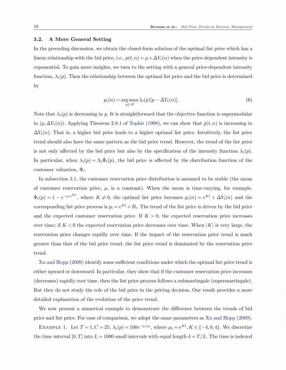
Example 1. Let T = 1,C = 25, λt(p) = 100e−p/µt , where µt = eKt,K ∈ −4,0,4. We discretize

the time interval [0, T ] into L= 1000 small intervals with equal length δ= T/L. The time is indexed


Figure 1 Bid Prices versus List Prices

0 0.2 0.4 0.6 0.8 10

0.2

0.4

0.6

0.8

1

1.2

1.4

Time t

Price

Bid Price Bt

List Price pt

(a) µt decreases rapidly (K =−4)

0 0.2 0.4 0.6 0.8 10.2

0.4

0.6

0.8

1

1.2

1.4

1.6

Time t

Price

Bid Price Bt

List Price pt

(b) µt stays constant (K = 0)

0 0.2 0.4 0.6 0.8 10

10

20

30

40

50

60

Time t

Price

Bid Price Bt

List Price pt

(c) µt increases rapidly (K = 4)

by t ∈ 0, δ,2δ, . . . ,Lδ. We first compute the optimal list price and bid price. Then, we simulate

the demand arrival in each interval [jδ, (j+1)δ] by a Bernoulli random variable with mean λ(jδ)δ,

j = 0, . . . ,L − 1 and the customer reservation price upon an arrival by an exponential random

variable with mean µ(jδ). We record all the trajectories of bid prices and list prices along the

simulated sample paths and calculate their means.

Figure 1 shows that the average sample paths of bid prices first move upward and then move

downwards while the optimal list price processes have different patterns. In particular, when the

expected customer reservation price falls rapidly, the average list price decreases over time (see

(a)). When the expected customer reservation price is constant over time, the average list price has

the same trend as the average bid price (see (b)). When the expected customer reservation price

increases rapidly, the average list price increases over time (see (c)). Observe that, in all cases, the

average bid price paths are rather “flat”. This implies that the trend of the expected reservation

price dominates the evolution of the list price process. These observations justify our theoretical

predictions.

3.3. Fluid Approximation and Martingale

Xu and Hopp (2006) provide a closed-form solution in a stochastic flow RM model with an iso-

elastic demand function and show that the optimal price process is a martingale. It is not hard

to show that with an iso-elastic demand function (i.e., λt(p) = Λtp−α, α > 1) the optimal price is

linear in the bid price (pt =α

α−1Bt where Bt is the bid price). This implies that the bid price is

also a martingale in Xu and Hopp’s model. They argue that the martingale list price process in

the stochastic fluid model (Xu and Hopp 2006) and the submartingale price process in the discrete

state system (Xu and Hopp 2009) are due to the nature of the customer arrivals: on the one hand,

because the flow demand model with the customer arrival rate being a geometric Brownian motion

always provides a positive customer flow, the seller can count on future customer arrivals; on the


other hand, with Poisson demand arrivals, the seller is not certain that there will be incoming

customers, and hence tends to set price lower at the beginning of the selling season. However, this

cannot explain the downward trend of the price process as shown in Xu and Hopp (2009). In the

following discussion, we provide an alternative interpretation from the bid price perspective.

Note that bid price or shadow price measures the marginal loss or opportunity cost of reducing

one unit of inventory. When the inventory level at time t is n, the marginal contribution of having

one more unit of inventory can be measured by ∆Vt(n+1) = Vt(n+1)−Vt(n). The next proposition

characterizes the trend of the marginal contribution of having one more unit of inventory.

Proposition 4. For any t∈ [0, T ) and s∈ (t, T ], ∆Vt(Nt +1)≥E[∆Vs∧τ0(Ns∧τ0 +1) |Ft].

This proposition shows that the marginal contribution of having one more unit of inventory

has a downward trend. This implies that the value of having more inventories declines over time.

Next, we use this proposition to give an explanation for the reason that the bid price in a fluid

approximation model becomes a martingale.

In the fluid approximation (see, e.g., Xu and Hopp 2006), the bid price of a resource is represented

by the derivative of the value function with respect to the inventory state. Let Vt(x) be the value

function of the fluid model where x represents the inventory level which is a continuous variable.

Suppose Vt(x) is differentiable in x. Then the bid price at time t is ∂∂xVt(x). Discretize the system

state by letting C =Mδ where M is a positive integer and assume that each customer demands

δ units. Then the bid price becomes Vt(x)− Vt(x− δ) and the marginal contribution of adding δ

more units of inventory becomes Vt(x+ δ)−Vt(x). Similarly to Theorem 1, we can show that the

bid price process in above discretized system first moves upwards and then move downwards after

the inventory falls to δ. Applying Proposition 4, we know that the process associated with the

marginal contribution of having δ more units of inventory has a downward trend. As δ→ 0, both

Vt(x)−Vt(x−δ)

δand Vt(x+δ)−Vt(x)

δconverge to ∂

∂xVt(x). Then,

∂∂xVt(x) is both a supermartingale and a

submartingale, and hence a martingale.

Now if we change the iso-elastic demand function in Xu and Hopp (2006) to an exponential

demand function as discussed in the previous subsection, i.e., λt(p) = Λe−p/µt where µt = eKt and

K is a constant, then the optimal list price becomes pt(x) = eKt + ∂∂xVt(x). Since the bid price

process is an martingale (in the fluid model), the list price process is a submartingale as K > 0, a

supermartingale as K < 0, and a martingale as K = 0. Thus, even the bid price process of the fluid

model is a martingale, the list price process is not necessarily a martingale.

The preceding analysis implies that the martingale property of the bid price process in the

fluid model is due to the smoothness of the system state. Since the inventory can be sold with


any small amount, the bid price has the same probability of moving upward (due to resource

scarcity) and moving downward (due to resource perishability) over time. However, in a discrete

state system where each sale of inventory yields a jump in the system state, the resource scarcity

and resource perishability may have opposite effects on the bid price movements. As we show in the

previous subsections, the resource scarcity effect dominates the movement of the bid price before

the inventory falls to one and the resource perishability effect dominates the movement of the bid

price afterwards. Therefore, the bid price process is not necessarily a martingale in the discrete

system.

3.4. Bounds and Heuristics

It is known that fixed-price heuristics of the deterministic fluid model can provide an upper bound

on the expected revenue of the stochastic model and the approximation is provably good when the

volumes of expected sales and capacity are large (Gallego and van Ryzin 1994). In this subsection,

we show that the bid price of the deterministic model provides a lower bound on the bid price of

the stochastic model.

Consider the following deterministic setting: At time t ∈ [0, T ), the remaining inventory level is

x, a continuous variable, the instantaneous demand rate is a deterministic function of price, i.e.,

λs(p) = Λse−p/µ for s∈ [t, T ), the pricing policy is pt, and the allowable price set is [0,∞).

The firm’s problem is to maximize the total revenue over [t, T ] given an inventory level x at time

t, denoted by Jt(x).

Jt(x) = maxps≥0,s∈[t,T )

∫ T

t

Λse−ps/µpsds

subject to

∫ T

t

Λse−ps/µds≤ x.

Gallego and van Ryzin (1994) show that a static pricing policy is optimal. Thus, the above problem

is equivalent to the following static optimization problem:

Jt(x) =maxp≥0

dte−p/µp

subject to dte−p/µ ≤ x,

where dt =∫ T

tΛsds. The optimal price, denoted by pt(x), and the associated bid price (Lagrange

multiplier), denoted by γt(x), given x, are obtained by solving the associated Lagrange problem:

minγ≥0

maxp≥0

dte−p/µp− γt(dte

−p/µ −x). (7)

Solving the problem yields pt(x) =maxµ log(dt/x), µ and γt(x) =maxµ(log(dt/x)− 1),0.

We next compare the bid price of the heuristic policy, γt, and the optimal bid price (5).


Figure 2 Heuristic Bid Price versus Optimal Bid Prices

0 0.1 0.2 0.3 0.4 0.5 0.6 0.7 0.8 0.9 10.2

0.25

0.3

0.35

0.4

0.45

0.5

0.55

0.6

0.65

0.7

Time t

Bid

Price

Bid Price: Bt ( =20, C=5)

Bid Price: Bt ( =200, C=50)

Bid Price: Bt ( =2000, C=500)

Heuristic Bid Price: 0(C)

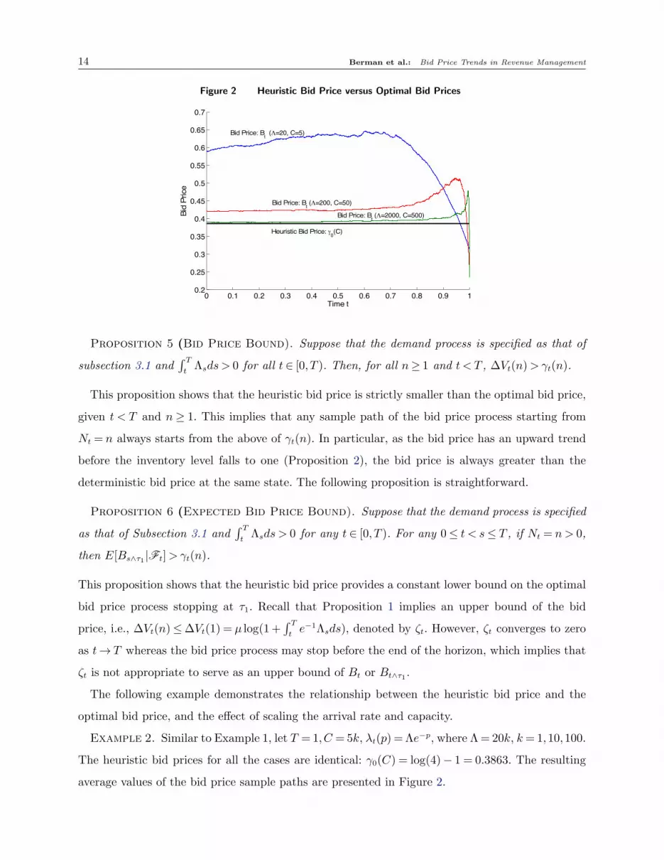
Proposition 5 (Bid Price Bound). Suppose that the demand process is specified as that of

subsection 3.1 and∫ T

tΛsds > 0 for all t∈ [0, T ). Then, for all n≥ 1 and t < T , ∆Vt(n)>γt(n).

This proposition shows that the heuristic bid price is strictly smaller than the optimal bid price,

given t < T and n≥ 1. This implies that any sample path of the bid price process starting from

Nt = n always starts from the above of γt(n). In particular, as the bid price has an upward trend

before the inventory level falls to one (Proposition 2), the bid price is always greater than the

deterministic bid price at the same state. The following proposition is straightforward.

Proposition 6 (Expected Bid Price Bound). Suppose that the demand process is specified

as that of Subsection 3.1 and∫ T

tΛsds > 0 for any t ∈ [0, T ). For any 0≤ t < s≤ T , if Nt = n > 0,

then E[Bs∧τ1 |Ft]> γt(n).

This proposition shows that the heuristic bid price provides a constant lower bound on the optimal

bid price process stopping at τ1. Recall that Proposition 1 implies an upper bound of the bid

price, i.e., ∆Vt(n)≤∆Vt(1) = µ log(1+∫ T

te−1Λsds), denoted by ζt. However, ζt converges to zero

as t→ T whereas the bid price process may stop before the end of the horizon, which implies that

ζt is not appropriate to serve as an upper bound of Bt or Bt∧τ1 .

The following example demonstrates the relationship between the heuristic bid price and the

optimal bid price, and the effect of scaling the arrival rate and capacity.

Example 2. Similar to Example 1, let T = 1,C = 5k, λt(p) = Λe−p, where Λ= 20k, k= 1,10,100.

The heuristic bid prices for all the cases are identical: γ0(C) = log(4)− 1 = 0.3863. The resulting

average values of the bid price sample paths are presented in Figure 2.


From Figure 2, we can observe that the heuristic bid price is lower than the optimal bid prices

when the bid prices move upwards, which verifies Proposition 6 that the optimal bid prices are

higher than the heuristic bid prices before the inventory levels fall to ones. Then the optimal

bid prices start falling quickly at the end of the horizon towards below the heuristic bid prices.

Comparing different demand-capacity combinations, it can be observed that the difference between

the optimal bid price and heuristic bid price becomes smaller when the market size and capacity are

scaled up. This is consistent with the result in Gallego and van Ryzin (1994) that the deterministic

fluid model provides a good approximation when the volume is large.

4. Quantity-Based Revenue Management

In the quantity-based RM models (see, e.g., Lautenbacher and Stidham 1999 and Feng and Xiao

2001), customers are segmented into several distinct fare classes with predetermined prices (fares).

An incoming booking request of a fare class is accepted only if its fare exceeds the bid price (or

opportunity cost) of the remaining inventory. This type of control is also called bid price control.

More specifically, we assume that there are K fare classes, indexed by i= 1, · · · ,K. The fare of

class k is pk which is fixed during the selling season. Without loss of generality, we assume that

0< p1 < p2 < · · ·< pK . Customer arrivals of fare class k follow a non-homogenous Poisson process

whose intensity at t is λkt > 0. The control is represented by u= (u1, . . . , uK) where

uk =

1 if booking request of class k is accepted,0 if booking request of class k is rejected.

The unit sales revenue of class k under a policy u is denoted by rkt (u). Then, rkt (u) =

pk if uk = 1,0 if uk = 0.

It follows by Feng and Xiao (2001) that the optimal revenue function, Vt(n), satisfies the following

HJB equation:

0 =∂Vt(n)

∂t+

K∑

k=1

λkt [pk −∆Vt(n)]

+, n≥ 0, (8)

with the boundary conditions Vt(0) = 0 and VT (n) = 0 for all t and n. The optimal policy is that

an incoming booking request of class k is accepted if and only if the corresponding fare is greater

than the bid price, i.e., pk >∆Vt(n). Note that the fare structure is nested, hence if a request of

class k < K is accepted, then all the requests from classes with higher fares should be accepted.

By Theorem 1, the optimal policy tends to reject more lower fare classes as time goes by before

the inventory level falls to one but afterwards it accepts more lower fare classes.

Although Feng and Xiao (2001) have shown that ∆Vt(n) is decreasing in t and n, we present a

stronger result which shows that the monotonicity of the bid price is strict.


Proposition 7 (Strict Monotonicity of Bid Price). For any t∈ [0, T ) and n> 0,

(i) ∆Vt(n+1)<∆Vt(n);

(ii) ∂∂t∆Vt(n)< 0.

Similar to Proposition 2, we have the following results.

Proposition 8 (Strict Bid Price Trends). For any t∈ [0, T ) and s∈ (t, T ],

(i) if Nt > 1, then Bt <E[Bs∧τ1 |Ft];

(ii) if Nt = 1, then Bt >E[Bs |Ft].

The strict inequalities imply that the optimal bid price process is neither a supermartingale nor

a submartingale, which shows that the bid price does not behave like a martingale. However, in

the fluid approximation models, the bid price process is indeed a martingale (Akan and Ata 2009).

Similar to the explanation in section 3, the smoothness of the fluid model equalizes the chances

of bid prices to move upwards and downwards. Akan and Ata (2009) also point out that the fluid

model provide a good approximation only for those systems with high demand and large capacity

such as call centers. For those systems with smaller capacity and demand (e.g., airlines and hotels),

the fluid approximation may cause significant revenue loss, which calls for better heuristics.

5. Concluding Remarks

In a general RM framework, we show that the optimal bid price (shadow price) has an upward

trend before the inventory level falls to one and has a downward trend afterwards. In particular,

in the price-based RM model, we show that the optimal list price is increasing in the bid price and

thus the upward/downward movement of optimal bid price may drive the the optimal list price

to move towards the same direction. In the special case with exponential demand intensity, we

show that the upward/downward trend is strict, which implies that the bid price process is not a

martingale. Analogous results are shown in a quantity-based RM model. In the online appendix,

we extend our analysis to the network RM models.

Our findings have important practical implications as the bid price is a fundamental factor

in determining the pricing or capacity allocation policy. Bid price control has become a popular

method in network RM (see, e.g., Talluri and van Ryzin 1998, Adelman 2007 and Topaloglu 2009).

A correct understanding of the rule governing the bid price is critical for designing heuristic or

approximation algorithms. The rule of bid price trend revealed in this note could serve as one of

the standards to examine bid price heuristics or approximations, especially for those systems with

relatively small capacity and demand.


References

Adelman, D. 2007. Dynamic bid-prices in revenue management. Oper. Res. 55(4) 647–661.

Akan M., B. Ata. 2009. Bid-price controls for network revenue management: Martingale characterization of

optimal bid prices. Math. Oper. Res. 34(4) 912–936.

Feng, Y., B. Xiao. 2000. A continuous-time yield management model with multiple prices and reversible

price changes. Management Sci. 46(5) 644–657.

Feng, Y., B. Xiao. 2001. A dynamic airline seat inventory control model and its optimal policy. Oper. Res.

49(6) 938–949.

Gallego, G., G. J. van Ryzin. 1994. Optimal dynamic pricing of inventories with stochastic demand over

finite horizons. Management Sci. 40(8) 999–1020.

Gallego, G., G. J. van Ryzin. 1997. A multiproduct dynamic pricing problem and its applications to network

yield management. Oper. Res. 45(1) 24–41.

Lautenbacher, C. J., S. Stidham Jr. 1999. The underlying Markov decision process in the single-leg airline

yield-management problem. Transportation Sci. 33(2) 136–146.

McAfee, R. P., V. te Velde. 2007. Dynamic pricing in the airline industry. T. J. Hendershott, ed. Handbook

on Economics and Information Systems. Elsevier, Amsterdam, 527–570.

Talluri, K. T., G. J. van Ryzin. 1998. An analysis of bid-price controls for network revenue management.

Management Sci. 44(11) 1577–1593.

Talluri K. T., G. J. van Ryzin. 2004. The Theory and Practice of Revenue Management. Kluwer, New York,

NY.

Topaloglu, H. 2009. Using lagrangian relaxation to compute capacity-dependent bid prices in network revenue

management. Oper. Res. 57(3) 637–649.

Topkis, D. M. 1998. Supermodularity and Complementarity. Princeton University Press, Princeton, NJ.

Xu, X., W. J. Hopp. 2006. Price trends in a dynamic pricing model with heterogenous customers: A martin-

gale perspective. Oper. Res. 57(5) 1298–1302.

Xu, X., W. J. Hopp. 2009. A monopolistic and oligopolistic stochastic flow revenue management. Oper. Res.

54(6) 1098–1109.


Zhao, W., Y. S. Zheng. 2000. Optimal dynamic pricing for perishable assets with nonhomogenous demand.

Management Sci. 46(3) 375–388.


This page is intentionally blank. Proper e-companion title

page, with INFORMS branding and exact metadata of the

main paper, will be produced by the INFORMS office when

the issue is being assembled.


Online Appendix to the Note

“On the Bid Price Trends in Revenue Management”

Oded Berman • Ming Hu

Rotman School of Management, University of Toronto, Toronto, ON M5S 3E6, Canada,

berman,[email protected]

Zhan Pang

Lancaster University Management School, Lancaster, LA1 4YX, United Kingdom,

[email protected]

Proof of Proposition 1

(i) To show that ∆Vt(n) is strictly decreasing in n for any t < T , it suffices to show that∑

n

i=0ait/i!∑n−1

i=0ait/i!

is strictly decreasing in n for all t < T , where at =∫ T

te−1Λsds. For any t < T , the assumption that

∫ T

tΛsds > 0 implies that at > 0. Then, for n≥ 1 and t < T ,

∑n+1

i=0 ait/i!

∑n

i=0 ait/i!

−

∑n

i=0 ait/i!

∑n−1

i=0 ait/i!

=an+1t /(n+1)!∑n

i=0 ait/i!

−ant /n!

∑n−1

i=0 ait/i!

=ant

n!

∑n−1

i=0at

n+1ait/i!−

∑n

i=0 ait/i!

∑n

i=0 ait/i!

∑n−1

i=0 ait/i!

≤ant

n!

∑n

i=1 ait/i!−

∑n

i=0 ait/i!

∑n

i=0 ait/i!

∑n−1

i=0 ait/i!

=ant

n!

−1∑n

i=0 ait/i!

∑n−1

i=0 ait/i!

< 0.

This proves that ∆Vt(n+1)<∆Vt(n);

(ii) As n= 1, ∆Vt(n) = Vt(1) = µ log(at). Taking derivative with respect to t yields

∂

∂t∆Vt(n) =−

µe−1Λt∫ T

te−1Λsds

≥ 0.

The inequality is strict if Λt > 0.

As n> 1, we have

∂

∂t∆Vt(n) = −µ

[

∑n−1

i=0 ait/i!

∑n

i=0 ait/i!

−

∑n−2

i=0 ait/i!

∑n−1

i=0 ait/i!

]

e−1Λt.

Similar to part (i), we can show that∑n−1

i=0ait/i!∑

n

i=0ait/i!

−∑n−2

i=0ait/i!

∑n−1

i=0ait/i!

> 0. As Λt ≥ 0, we have ∂∂t∆Vt(n)≤ 0.

The inequality is strict if Λt > 0. Q.E.D.

mailto:[email protected],[email protected]

mailto:[email protected]



As shown in Proposition 1, ∆Vt(n) is strictly decreasing in n for any t < T , which implies that

p(t, n) is strictly decreasing in n for all t < T . Moreover, the closed-form solution of ∆Vt(n) also

implies that ∆Vt(n)> 0 for all t < T . Then, under the constructed policy u in the proof of Theorem

1, we have Vt(Nt) < Vt(Nt) = Vt(Nt − 1) for all t < T . Similarly, under the constructed policy u,

we have Vt(1) < Vt(1). Applying the arguments of the proof of Theorem 1 leads to the desired

assertions. Q.E.D.


Similar to Theorem 1, we let u∗s(Ns) be the optimal control at time s∈ [t, T ]. Then, for Nt = n≥ 0

and t < s≤ T , by Bellman’s Principle of Optimality, we have

Vt(Nt) =E

[∫ s∧τ0

t

rξ−(u∗ξ(Nξ))dNξ +Vs∧τ0(Ns∧τ0)|Ft

]

(A1)

Now, construct a policy u such that

us(Ns) =

u∗s(Ns − 1) if t≤ s < τ0

u∗s(Ns) if τ0 ≤ s≤ T ,

where Ns : s∈ [t, T ] is the inventory process under u starting with Nt = n+1 and τ0 is the stopping

time when the optimal inventory level process starting with Nt = n first falls to zero. That is, the

constructed policy has the same control as that of the optimal control at the state of having one

unit of inventory less. Clearly, u∈U . Under the policy u, the intensity λξ(uξ(Nξ)) = λξ(u∗ξ(Nξ+1))

as s≤ τ0. Let Aξ =C − Nξ be the demand process under the policy u.

Recall that Nt = n and Nt = n+ 1. Along the same sample path of the incremental demand

process between t and s∧τ0, we have Nξ =Nξ+1 and λξ(uξ(Nξ)) = λξ(u∗ξ(Nξ)) for any ξ ∈ [t, s∧τ0).

In particular, Ns∧τ0 =Ns∧τ0 +1. Similarly, we have rξ−(uξ(Nξ)) = rξ−(u∗ξ(Nξ)) for any ξ ∈ [t, s∧τ1).

Let Vt be the expected revenue over [t, T ] under the policy u. It satisfies the following recursive

equation:

Vt(Nt) = E

[∫ s∧τ0

t

rξ−(uξ(Nξ))dNξ + Vs∧τ0(Ns∧τ1)|Ft

]

= E

[∫ s∧τ0

t

rξ−(u∗ξ(Nξ))dNξ +Vs∧τ0(Ns∧τ1 +1)|Ft

]

.

The suboptimality of Vt implies that Vt(Nt +1)≥ Vt(Nt) which infers that

Vt(Nt +1)≥E

[∫ s∧τ0

t

rξ−(u∗ξ(Nξ))dNξ +Vs∧τ0(Ns∧τ0 +1)|Ft

]

. (A2)

Subtracting both sides of (A1) from (A2) yields ∆Vt(Nt+1)≥E [∆Vs∧τ0(Ns∧τ0 +1)|Ft] . Q.E.D.



First, if dt ≤ n, then γt(n) = 0. Note that ∆Vt(n)> 0 as t < T and n > 0. Then, ∆Vt(n)> γt(n).

Now, suppose dt > n. Then γt(n) = µ log(∫ T

te−1Λsds/n). Let at =

∫ T

te−1Λsds. Since

∫ T

tΛsds > 0,

at > 0. Then, we have

∆Vt(n)− γt(n) = µ log

∑n

i=0 ait/i!

∑n−1

i=0 ait/i!

−µ log(at/n)

= µ log

∑n

i=0 ait/i!

∑n−1

i=0 (ait/i!)(at/n)

≥ µ log

∑n

i=0 ait/i!

∑n−1

i=0 (ai+1t /(i+1)!)

= µ log

∑n

i=0 ait/i!

∑n

i=1(ait/i!)

= µ log

1+1

∑n

i=1(ait/i!)

> 0.

This proves the proposition. Q.E.D.


The results are proved by induction. First, we argue that ∆Vt(n) < pK for any n ≥ 1, which is

trivially true since pK is the highest revenue the seller can obtain from a unit. Let λk(t, n) = λk if

pk >∆Vt(n) and λk(t, n) = 0 otherwise. Then, ∆Vt(n)< pK implies that λK(t, n) = λK for all t and

n.

Then, the proposition is proved by induction. If n= 1, applying (8) yields ∂Vt(n)

∂t< 0 for all t < T .

Now, suppose ∂∂t∆Vt(n)< 0 for n≥ 1. Applying (8) yields

0 =∂Vt(n+1)

∂t+

K∑

k=1

λk(t, n+1)[pk −∆Vt(n+1)],

0 ≥∂Vt(n)

∂t+

K∑

k=1

λk(t, n+1)[pk −∆Vt(n)],

where the inequality is because we substitute the optimal solution λk(t, n) with a supoptimal

solution λk(t, n+1). A substraction yields

0 ≤∂∆Vt(n+1)

∂t−

K∑

k=1

λk(t, n+1)[∆Vt(n+1)−∆Vt(n)].

By induction assumption ∂∂t∆Vt(n)< 0, we have

0 <∂[∆Vt(n+1)−∆Vt(n)]

∂t−

K∑

k=1

λk(t, n+1)[∆Vt(n+1)−∆Vt(n)],


=∂[(∆Vt(n+1)−∆Vt(n))e

∫T

t

∑K

k=1λk(s,n+1)ds]

∂t.

That is, (∆Vt(n+1)−∆Vt(n))e∫T

t

∑K

k=1λk(s,n+1)ds is strictly increasing in t < T . Note that ∆Vt(n+

1)−∆Vt(n) = 0. Then, (∆Vt(n+ 1)−∆Vt(n))e∫T

t

∑K

k=1λk(s,n+1)ds < 0, which implies that ∆Vt(n+

1)<∆Vt(n).

Applying (8) again yields

0 ≥∂Vt(n+1)

∂t+

K∑

k=1

λk(t, n)[pk −∆Vt(n+1)],

0 =∂Vt(n)

∂t+

K∑

k=1

λk(t, n)[pk −∆Vt(n)].

A subtraction leads to

0 ≥∂∆Vt(n+1)

∂t−

K∑

k=1

λk(t, n)[∆Vt(n+1)−∆Vt(n)],

which implies that

∂∆Vt(n+1)

∂t≤

K∑

k=1

λk(t, n)[∆Vt(n+1)−∆Vt(n)]< 0.

This completes the induction and proves the inequalities. Q.E.D.

Extension: Bid Price Trends in Network Revenue Management

Consider an airline network consisting of I legs, indexed by i= 1, · · · , I, and J original-destination

itineraries, indexed by j = 1, · · · , J , which can be treated as a multi-product system where each

product is corresponding to an itinerary and each resource is corresponding to a leg. The initial

capacity of resource i is Ci. Define the vector C = (C1, . . . ,CI)′ ∈ Z

I+. Product j includes qij units

of capacity of resource i. Let Q= [qij], qij ∈ 0,1. Assume that Q is integer valued and has no zero

columns; that is, each product consists of at least one unit of capacity of one of I resource. The

jth column of Q, Qj, is the incidence vector for itinerary j. If i∈Qj, then product j uses leg i. At

any time t∈ [0, T ], let Ni(t) be the remaining capacity level of leg i. Let N(t) = (N1(t), · · · ,NI(t)).

The state of the network is the available capacity denoted by a vector n= (n1, · · · , nI)∈ZI+.

The demands arrive as a J-variate point process defined on a measurable space (Ω,F ) with the

intensity λjt(u) for itinerary j, j = 1, · · · , J , where u is an admissible policy in an admissible set U .

Let At = (A1t , · · · ,A

Jt )

′, where Ajt is the total number of sales of product j up to time t. Assume

that, for any given u, λjt(u) is independent of At. The unit revenue from a sale of product j at time


t under the policy u is denoted by rjt−(u) ∈ [0,∞). Let rt−(u) = (r1

t−(u), · · · , rJ

t−(u)). The firm’s

problem is

maxu∈U

E

[∫ T

0

rs−(u)dAs|Ft

]

subject to∫ T

0QdAs ≤C.

Let u∗ be the optimal policy. Given the inventory levels n at time t, the expected revenue over

period [t, T ] under the optimal policy is

Vt(n) =E

[∫ T

t

rs−(u∗)dAs|Ft

]

.

Note that VT (n) = 0 for any n and Vt(0) = 0 for any t, where 0 is a I-dimensional vector with all

the elements being zeros.

Define ∆iVt(n)≡ Vt(n)− Vt(n− ei) as the bid price (shadow price) of the inventory of i-th leg

at time t, where ei is a I-dimensional unit vector with a one in the ith element. Let τ im ≡ inft ∈

[0, T ]|maxj Kijt =m be the earliest time that the maximum inventory level of the products that

contain resource i falls to m≤ C, where Kijt =minkNk(t) : qkj = 1 and qij = 1 is the maximum

available inventory level of product j that contains resource i. As each product may consist of

several resources, the effectiveness of the inventory of a resource depends on the inventories of

other resources that can be combined into a product. Note that Kijt > 1 implies that Ni(t)> 1, but

Ni(t)> 1 does not imply that Kijt > 1. The term maxj K

ijt represents the effective inventory level

of resource i at time t, i.e., the maximum amount of products that the resource i can contribute

to. If maxj Kijt = 1 and Ni(t)> 1, then Vt(N(t)) = Vt(N(t)− ei), i.e., ∆

iVt(N(t)) = 0. Similarly, if

maxj Kijt = 0 and Ni(t)> 0, then Vt(N(t)) = Vt(N(t)− ei), i.e., ∆

iVt(N(t)) = 0.

Given the demand process Nt, the optimal bid price process of the ith leg capacity can be defined

as

Bit ≡∆iVt∧τ i

0−(Nt∧τ i

0−).

Theorem 2 (Bid Price Trends). Given the inventory vector n at time t, for any t < s≤ T ,

(i) if maxJj=1K

ij(t)> 1, then Bt ≤E[Bs∧τ1 |Ft];

(ii) if maxJj=1K

ij(t) = 1, then Bt ≥E[Bs |Ft].

The proof follows the same procedure as that of Theorem 1. That is, for the first assertion, we

construct a policy such that before the random time τ im, the system behaves under the optimal

policy as if there is one more unit of resource i. That is, the decision at each state is taken to

be equal to the decision at the state having one more unit of inventory. The second assertion is

straightforward.


Similar to Theorem 1, Theorem 2 shows that the bid price of a resource has an upward trend

before the effective inventory level of this resource falls to one and a downward trend afterwards.

This implies that the bid price process may not be a semi-martingale or a martingale as suggested

in those fluid approximation models (see, e.g., Akan and Ata 2009). Although the fluid model can

provide a good approximation in the environments (e.g., call centers) with high demands and large

capacities (Gallego and van Ryzin 1997, Talluri and van Ryzin 1998), it may not guarantee a good

performance in the environments with relatively small capacities and low but volatile demands

(e.g., airlines and hotels). However, the multidimensional nature of the network problem leads

to the curse of dimensionality in computation and analysis. Recent developments in approxima-

tion dynamic programming (ADP) attempt to improve the computational performances (see, e.g.,

Adelman 2007, Topaloglu 2009). The key idea is to approximate the value function in order to

generate bid prices. Without computing the optimal policy (which is not tractable), a straight way

to examine the performance of ADP is to compare the expected revenue under the policy derived

from ADP with that of the fluid model. Since our result fits the intuition, it may serve as another

reference point to examine whether the bid price derived from ADP is consistent with the intuition:

The average sample paths of the bid price should have an upward trend at the beginning of the

selling season and will move downward at the end of the selling season.

References

Adelman, D. 2007. Dynamic bid-prices in revenue management. Oper. Res. 55(4) 647–661.

Akan M., B. Ata. 2009. Bid-price controls for network revenue management: Martingale characterization of

optimal bid prices. Math. Oper. Res. 34(4) 912–936.

Gallego, G., G. J. van Ryzin. 1997. A multiproduct dynamic pricing problem and its applications to network

yield management. Oper. Res. 45(1) 24–41.

Talluri, K. T., G. J. van Ryzin. 1998. An analysis of bid-price controls for network revenue management.

Management Sci. 44(11) 1577–1593.

Topaloglu, H. 2009. Using lagrangian relaxation to compute capacity-dependent bid prices in network revenue

management. Oper. Res. 57(3) 637–649.

On the Bid Price Trends in Revenue Management

Documents

Transcript of On the Bid Price Trends in Revenue Management