On Pollution Permit Banking and Market Power

Matti Liski and Juan-Pablo Montero∗

February 8, 2005

Abstract

We consider a pollution permits market in which there are a large polluting firm

plays and a fringe of competitive firms. To smooth compliance towards the long-

run emissions goal, firms are initially allocated a stock (i.e., bank) of permits to

be gradually consumed. We first show how the large firm can credibly manipulate

the spot market in subgame-perfect equilibrium. Motivated by features observed

in the market for sulfur dioxide emissions of the US Acid Rain Program, we then

show that the introduction of stock transactions has no effects on market power,

but that forward trading and incomplete observability of stock holdings do have

pro-competitive effects.

JEL classification: L51; Q28.

1 Introduction

Pollution permit markets are usually about trading across space in the same period, but

they can also entail trades over time. Typically, permit market designs allow intertempo-

ral trading in the form of banking which means that unused permits in one period can be

saved and used in later periods. Over the past decade, this latter dimension of pollution

∗Liski (liski@hkkk.fi) is at the Economics Department of the Helsinki School of Economics and Mon-tero (jmontero@faceapuc.cl) is at the Economics Department of the Catholic University of Chile (PUC).Both authors are also Research Associates at the MIT Center for Energy and Environmental PolicyResearch. Liski thanks funding from the Nordic Energy Research Program and the Academy of Finlandand Montero from Fondecyt Grant No. 1030961.

1

permit trading has drawn increasing attention in the literature, and proposals to decrease

emission caps over time suggest a particular larger role for banking in the future. The

most prominent example is the US Acid Rain Program, where banking has been a major

form of permit trading (Ellerman et al., 2000; Ellerman and Montero, 2005). During

the first five years of the program constituting Phase I, 1995-99, only 26.4 million of the

38.1 million permits (or allowances) distributed were used to cover sulfur dioxide (SO2)

emissions. The remaining 11.65 million allowances (30% of all the allowances distributed)

were banked and have been gradually consumed during Phase II (2000 and beyond). As

a result, the Phase II emissions cap is expected to be reached at some time between 2008

and 2010.

Several authors have studied the theoretical properties of pollution permit banking

(e.g., Rubin, 1996; Cronshaw and Kruse, 1996; Schennach, 2000), but there is little work

on the effect of market power on the equilibrium banking path.1 We believe it is important

to fill this gap not only for a better understanding of the performance of the existing

markets for which banking is relevant but also for the better design (including permit

allocations) of similar markets in the future. In that respect, the US Acid Rain Program

appears as an interesting case study provided that we observe a substantial amount of

banking and that large fraction of the permits are in the hands of few holding companies.

An eventual carbon market with declining emission targets (and economic growth) is

another relevant example. There are simulation studies documenting the possibility for

large players (i.e., countries) to move the market away from the perfectly competitive

outcome (e.g., Ellerman and Wing, 2000; Maeda, 2003), but these studies have adopted a

static view of the problem in that firms are not allowed to trade permits intertemporally.

It is not clear how those results would change with banking. The introduction of permit

banking produce a significant increase in the liquidity of the market by making permits

from previous vintages available for compliance in a given year. Some may argue that

this market expansion would necessarily make the market more competitive while others

may suggest the opposite, that banking creates opportunities for firms to expand their

market power, for example, by buying large fractions of the overall permit stock.

1Hahn (1984) is the first to study market power in a permit market, but he considers a static context.

2

These questions call for a more formal analysis. One of the few attempts in that

direction is Liski and Montero (2004).2 They consider the presence of a large (polluting)

firm or a cohesive cartel and a fringe of competitive firms and discuss the conditions

that hold in equilibrium for very particular permits allocations. They find, for example,

that a large firm receiving no stock allocation of permits (only a flow allocation) finds it

optimal to follow competitive pricing during the banking path. That study, however, has

some important limitations. It does not provide a general solution for the equilibrium

path for any permits allocations and restricts the analysis to spot transactions.

In this paper, we build upon Liski and Montero (2004) and describe the subgame-

perfect equilibrium for any permit allocations between the large firm and the fringe.

This benchmark model is then used to identify the effects of stock transactions (either by

regulated firms or nonregulated outsiders), forward trading, and incomplete observability

of (actual) permit holdings. These are features that we observe in the US SO2 trading

program, and their implications for market power have not been analyzed before.

Because the evolution of the stock or bank of permits is closely related to the evolution

of an exhaustible resource, we draw upon both the literature on permits markets and the

literature on exhaustible resources to discuss whether and how the large (potentially

dominant) firm can affect the equilibrium path. Yet, there are important differences

between a permit market and a market for an exhaustible resource. For example, the

permits market still remains after the permits bank has been exhausted while the market

for an exhaustible resource vanishes after the total stock has been consumed. In addition,

the demand for permits corresponds to a derived demand from the same firms that hold

the permits while the demand for a typical exhaustible resource comes from a third party.

This implies that firms have the opportunity to buy permits if they wish to increase their

stock of permits; something that by construction is ruled out in depletable resource

models. In any case, these differences make the intertemporal permit market unique and

interesting.

2Hagem and Westskog (1998) also consider market power in an intertemporal permit market. How-ever, their two-period approach could not be used to analyze the issues raised here. Using a multiple-period horizon, Bernard et al.(2003) also introduce banking into a carbon trading regime but theirequilibrium solution is based on a dynamic optimization approach that is quite different from our game-theorical approach.

3

The rest of the paper is organized as follows. In Section 2, we develop a four-period

model and limit attention to spot transactions. In Section 3, we explore how the equilib-

rium path found in Section 2 changes when firms can also be engaged in stock transactions

(i.e., buy or sell permits beyond those needed or unneeded for current compliance). In

Section 3, we study the effect of forward transactions on the equilibrium path. In Section

4, we discuss the implications of imperfect observability of firms stock holdings on the

equilibrium path. Final remarks are in Section 5.

2 The Model

Since the permits bank is a depletable stock just like any other non-renewable resource,

it is reasonable to believe that the equilibrium depletion path cannot be too different

from the equilibrium path for a typical non-renewable resource. Thus, to find the bank-

ing equilibrium path we start by imposing the equilibrium characterization spelled out

by Salant (1976) and then check that such characterization is indeed the equilibrium

solution for the permit banking problem as well. The Salant’s (1976) depletion path is

characterized by two distinct phases. During the first or competitive phase numerous

small firms (competitive fringe) deplete their stocks. During the second or monopoly

phase, which starts right after the exhaustion of the fringe’ stock, the single large firm

(or cohesive cartel) is the only stockholder in the market. The banking path ends with

the exhaustion of the large firm’ stock. The long-run or after-banking equilibrium can

also be subject to market manipulation by the large firm from the strategic choice of its

abatement and permit sales/purchases (Hahn, 1984).

To study the exercise of market power during and after the banking period in the

simplest way, we construct a four-period model (t = 1, 2, 3, 4). The fringe is holding a

permit stock in periods 1 and 2; the large firm is the monopoly stockholder in period

3; and the long-run (Hahn) equilibrium arrives in period 4 in which no stocks are left.

Before explaining the four periods in detail, we introduce the allocations, technologies,

and timing assumptions for the game.

The large firm (indexed by m) and the fringe (indexed by f) receive constant flow

4

allocations (am, af) per period. They also receive initial stock allocations denoted by

(sm0 , sf0).

3 We rule out the borrowing of permits: current permit vintages as well as

previous vintages in stocks can be saved for use in any later periods but future permits

vintages cannot be used today. We adopt the convention that sit is the amount of stock

held by group i = m, f at the end of period t, i.e., after trading and emission decisions

for period t have been undertaken, stock sit is available in period t + 1. We assume for

now that individual stock holdings are publicly observed (later we relax this assumption).

The amount of permits sold (bought) by i in t (a negative value indicates a net purchase)

is denoted by xit, and the market clearing price of permits in period t is pt. r denotes the

discount rate common to all firms.

In the absence of regulation, group i’s unrestricted emissions are ui > ai per period

(the flow allocations are assumed to be binding). The aggregate abatement in period t

for group i is denoted by qit, so that emissions per period are eit = ui − qit. We assume

that total abatement costs of group i is given by time-invariant abatement cost function

Ci(qit), satisfying strict convexity assumptions: C(0) = 0, C

0i(q

it) > 0,and C 00

i (qit) > 0.

Let us now discuss the game between the two groups of agents, i.e., the large firm

and the fringe. Both groups have rational expectations but only the large firm behaves

strategically taking into account the effect of its own actions on the market equilibrium.

Each firm in the fringe, on the other hand, is so small that it takes prices as given. Thus,

we take the fringe as a rational-expectations, price-taking unit. We view the large firm as

a Stackelberg leader in the sense that it moves first in each spot market t. More precisely,

the large firm decides for period t the number of permits xmt to be sold (bought) in the

market. The market does not observe its level of abatement qmt (this is only observed

at the end of the compliance period, i.e., after the spot market has cleared). But since

the market can (perfectly) infer qmt from the observation of xmt and the current stock

holdings, we can assume that both qmt and xmt are simultaneously chosen by the large

firm.

Having observed the amount of permits offered (ordered) by the large firm, small

3The stock allocations can be created by a multi-period phase of generous flow allocations as in theU.S. Acid Rain program. Without losing any generality we do not explicitly model the initial savingphase of permits that leads to these initial stocks (see Liski and Montero, 2004).

5

firms decide their abatement levels and trade to clear the permits market. While the

market clearing price at t will be directly related to the fringe’s current abatement level

qft , the latter will, in turn, depend on the fringe’s expectations about the evolution of

the market in subsequent periods. For example, fringe members will make faster use of

their stock of permits and abate less if they expect the future price of permits to drop in

present value terms. Likewise, they will tend to hold onto their permits and abate more

if they expect the future price to increase in present value terms. In equilibrium, fringe

members correctly anticipate the evolution of market prices, hence, prices must exactly

rise at the rate of interest during the period in which the fringe is holding a stock of

permits.

The subgame perfect equilibrium of the game is found by backward induction. Hence,

in what follows for the rest of the section we will first derive the equilibrium conditions

after the exhaustion of the bank of permits (long-run equilibrium), then the equilibrium

conditions when the only stockholder is the large firm (monopoly sotckholder phase), and

finally, the equilibrium conditions when both the large firm and the fringe are holding

stocks of permits (competitive phase).

2.1 Long-run equilibrium

We assume that the initial permit stocks are such that the long-term abatement goal is

reached in period t = 4. That is, the stock of permits is consumed within the first three

periods, so that in the fourth period, em4 + ef4 = am + af . Then, if at the beginning of

t = 4, the large firm and the fringe have no stocks, sm3 = sf3 = 0, the problem for the

large firm is to maximize the net revenue from permit sales and compliance costs subject

to the constraint that sales can be made only by abating more than what is the minimum

abatement requirement um − am in this period.

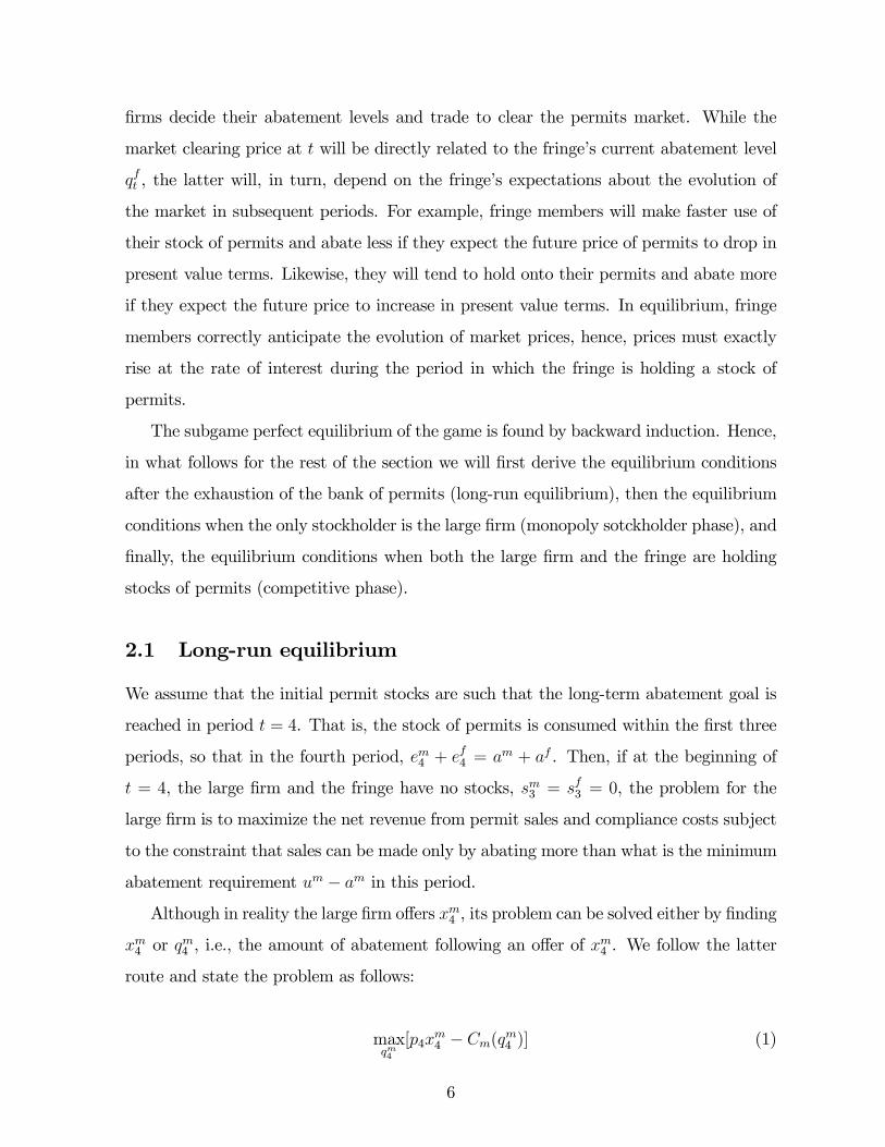
Although in reality the large firm offers xm4 , its problem can be solved either by finding

xm4 or qm4 , i.e., the amount of abatement following an offer of x

m4 . We follow the latter

route and state the problem as follows:

maxqm4[p4x

m4 − Cm(q

m4 )] (1)

6

where

p4 = C 0f(q

f4 ) (2)

xm4 = qm4 + am − um (3)

xf4 = qf4 + af − uf (4)

xf4 + xm4 = 0 (5)

Equation (2) indicates that in equilibrium fringe members reduce emissions to the point

where the cost of an extra unit of abatement is equal to the permits price. Eqs. (3)

and (4) capture the full compliance status of all firms, and eq. (5) is a market clearing

condition.

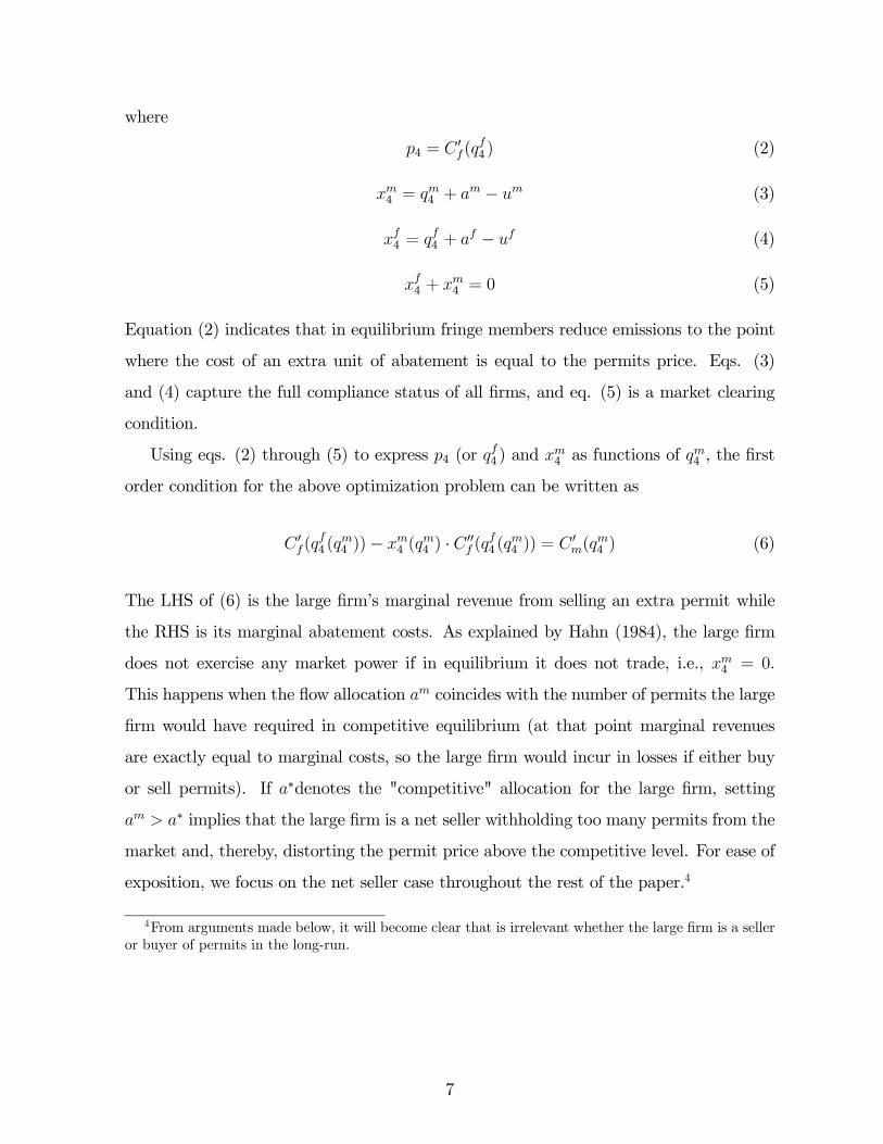
Using eqs. (2) through (5) to express p4 (or qf4 ) and xm4 as functions of q

m4 , the first

order condition for the above optimization problem can be written as

C 0f(q

f4 (q

m4 ))− xm4 (q

m4 ) · C 00

f (qf4 (q

m4 )) = C 0

m(qm4 ) (6)

The LHS of (6) is the large firm’s marginal revenue from selling an extra permit while

the RHS is its marginal abatement costs. As explained by Hahn (1984), the large firm

does not exercise any market power if in equilibrium it does not trade, i.e., xm4 = 0.

This happens when the flow allocation am coincides with the number of permits the large

firm would have required in competitive equilibrium (at that point marginal revenues

are exactly equal to marginal costs, so the large firm would incur in losses if either buy

or sell permits). If a∗denotes the "competitive" allocation for the large firm, setting

am > a∗ implies that the large firm is a net seller withholding too many permits from the

market and, thereby, distorting the permit price above the competitive level. For ease of

exposition, we focus on the net seller case throughout the rest of the paper.4

4From arguments made below, it will become clear that is irrelevant whether the large firm is a selleror buyer of permits in the long-run.

7

2.2 Monopoly stockholder phase

We consider now the last period of the banking phase, period 3, in which only the large

firm is holding a stock. To see why it must be the case that the large firm is the sole

stockholder in the end of a noncompetitive depletion path, recall that in competitive

equilibrium prices would grow at the rate of interest as long as some stocks are left for

the next period so that the competitive agents are willing to hold stocks to the end of the

depletion path. Thus, if the competitive agents are the last stockholders, then the price

path must be competitive throughout. In the noncompetitive stock-depletion equilibrium,

the large firm is the last stockholder equalizing present-value marginal revenues across

periods, implying that prices grow at a lower than the interest rate so that the competitive

agents are indeed willing to exhaust their stocks before the monopoly stockholder phase.

This decline in the present-value prices can occur only in the end of the path because of

the fringe arbitrage (see also Salant, 1976; and Newbery, 1981).

At the beginning of t = 3, the large firm has a stock of sm2 and the fringe has a stock

of sf2 = 0, coming from the earlier period. Taking sm2 > 0 and sf2 = 0 as given, the large

firm solves

πm3 (sm2 ) = max

qm3[xm3 p3 − Cm(q

m3 )] (7)

where

p3 = C 0f(q

f3 ) (8)

xm3 = sm2 + qm3 + am − um (9)

xf3 = qf3 + af − uf (10)

xf3 + xm3 = 0 (11)

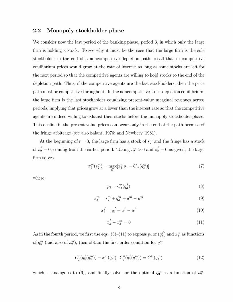
As in the fourth period, we first use eqs. (8)—(11) to express p3 or (qf3 ) and x

m3 as functions

of qm3 (and also of sm2 ), then obtain the first order condition for q

m3

C 0f(q

f3 (q

m3 ))− xm3 (q

m3 ) · C 00

f (qf3 (q

m3 )) = C 0

m(qm3 ) (12)

which is analogous to (6), and finally solve for the optimal qm3 as a function of sm2 .

8

Having obtained qm3 = qm3 (sm2 ), we then obtain equilibrium values for p3(s

m2 ) and x

m3 (s

m2 ).

Replacing these equilibrium values in the objective function, we can define

πm3 (sm2 ) = p3(s

m2 ) · xm3 (sm2 )− Cm(q

m3 (s

m2 )) (13)

as the subgame-perfect equilibrium profit that the large firm will obtain if the stocks

left at the end of the second period are sf2 = 0 and sm2 . Recall, that this construction

assumes that the price at t = 3 is lower than the price at t = 2 in present value terms

(i.e., p2 > p3/(1 + r)), otherwise there would be no monopoly phase at t = 3.

2.3 Competitive phase

We are now in the competitive phase where both the large firm and the fringe hold a

stock of permits. Let us first consider the last period of this competitive phase, that

is, period 2. At the beginning of t = 2, the large firm has a stock of sm1 and the fringe

has stock sf1 > 0. Because now the large firm must also decide about the amount of

stock to be left for the third period, its sales xm2 is not only a residual determined by its

abatement qm2 , as in the last two periods. Therefore, taking sm1 and s

f1 as given, the large

firm chooses both qm2 and xm2 to solve

πm2 (sm1 , s

f1) = max

qm2 ,xm2[xm2 p2 − Cm(q

m2 ) +

πm3 (sm2 )

1 + r] (14)

where

p2 = C 0f(q

f2 ) (15)

sm2 = sm1 + am + qm2 − xm2 − um (16)

sf2 = sf1 + af + qf2 − xf2 − uf = 0 (17)

xf2 + xm2 = 0 (18)

and πm3 (sm2 ) is given by (13).

The large firm’s problem is to determine how much to save of its remaining stock sm1

to the next period. Intuitively, since the marginal revenue gives the opportunity cost of

9

using permits for own compliance, the two should be equal in all periods. Moreover, if

the marginal revenue in one period is higher than in other, the allocation of the stock

usage over time can be improved. In Appendix A we show that the first order conditions

for qm2 and xm2 are given by

−C 0m(q

m2 ) +

C 0m(q

m3 )

1 + r= 0 (19)

C 0f(q

f2 )− xm2 C

00f (q

f2 )−

C 0m(q

m3 )

1 + r= 0 (20)

Equilibrium condition (19) implies compliance cost minimization during the banking

equilibrium: the large firm’s marginal abatement costs rise at the rate of interest. Condi-

tion (20) implies that the marginal revenue from selling a permit is equal to the marginal

cost of abatement. Combining the two implies that both marginal costs and revenues

grow at the rate of interest during the banking phase.

Having found the subgame-perfect equilibrium values qm2 = qm2 (sm1 , s

f1) and xm2 =

xm2 (sm1 , s

f1), we can compute p2(s

m1 , s

f1) and s

m2 (s

m1 , s

f1). Replacing these equilibrium values

in the objective function we define

πm2 (sm1 , s

f1) = xm2 (s

m1 , s

f1)p2(s

m1 , s

f1)− Cm(q

m2 (s

m1 , s

f1)) +

πm3 (sm2 )

1 + r. (21)

as the subgame-perfect equilibrium profit that the large firm will receive if the stocks left

at the end of the first period are sm1 > 0 and sf1 > 0.

Finally, at the beginning of t = 1, the large agent and the fringe have initial stocks

of sm0 and sf0 , respectively. Taking these stocks as given, the large agent solves

πm1 (sm0 , s

f0) = max

qm1 ,xf1

[xm1 p1 − Cm(qm1 ) +

πm2 (sm1 , s

f1)

1 + r] (22)

where

p1 = C 0f(q

f1 ) (23)

sm1 = sm0 + am + qm1 − xm1 − um (24)

10

sf1 = sf0 + af + qf1 − xf1 − uf (25)

xf1 + xm1 = 0 (26)

p1 =p2(s

m1 , s

f1)

1 + r(27)

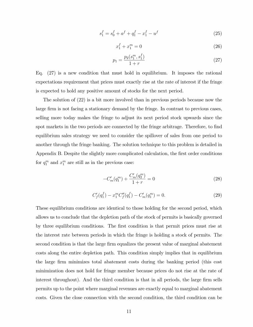
Eq. (27) is a new condition that must hold in equilibrium. It imposes the rational

expectations requirement that prices must exactly rise at the rate of interest if the fringe

is expected to hold any positive amount of stocks for the next period.

The solution of (22) is a bit more involved than in previous periods because now the

large firm is not facing a stationary demand by the fringe. In contrast to previous cases,

selling more today makes the fringe to adjust its next period stock upwards since the

spot markets in the two periods are connected by the fringe arbitrage. Therefore, to find

equilibrium sales strategy we need to consider the spillover of sales from one period to

another through the fringe banking. The solution technique to this problem is detailed in

Appendix B. Despite the slightly more complicated calculation, the first order conditions

for qm1 and xm1 are still as in the previous case:

−C 0m(q

m1 ) +

C 0m(q

m2 )

1 + r= 0 (28)

C 0f(q

f1 )− xm1 C

00f (q

f1 )− C 0

m(qm1 ) = 0. (29)

These equilibrium conditions are identical to those holding for the second period, which

allows us to conclude that the depletion path of the stock of permits is basically governed

by three equilibrium conditions. The first condition is that permit prices must rise at

the interest rate between periods in which the fringe is holding a stock of permits. The

second condition is that the large firm equalizes the present value of marginal abatement

costs along the entire depletion path. This condition simply implies that in equilibrium

the large firm minimizes total abatement costs during the banking period (this cost

minimization does not hold for fringe member because prices do not rise at the rate of

interest throughout). And the third condition is that in all periods, the large firm sells

permits up to the point where marginal revenues are exactly equal to marginal abatement

costs. Given the close connection with the second condition, the third condition can be

11

also interpreted as that in equilibrium the large firm’s marginal revenues must rise at the

rate of interest along the entire depletion path.

2.4 Discussion

In the subgame-perfect equilibrium that we have just characterized, the evolution of

prices must satisfyp4

(1 + r)3<

p3(1 + r)2

<p2

(1 + r)= p1. (30)

This price path does not necessarily hold for any arbitrary partition of the initial stock

between the large firm and the fringe. Implicit constraints on stockholdings are needed to

facilitate the four period exposition which we want to keep for simplicity.5 We illustrate

these constraints as well as the nature of the equilibrium by the following numerical

example. Let us assume that unrestricted emissions are um = uf = 10 and that flow

allocations are am+af = 10, so the regulator’s long-term goal is to halve total emissions.

To allow firms for a gradual transition to this long-term goal, the regulator provides a

stock of 10 to be allocated between the large firm and fringe members. Abatement cost

curves are Cf(qf) = 1

2(qf)2 and Cm(q

m) = 12(qm)2. The discount rate is r = 0.5.

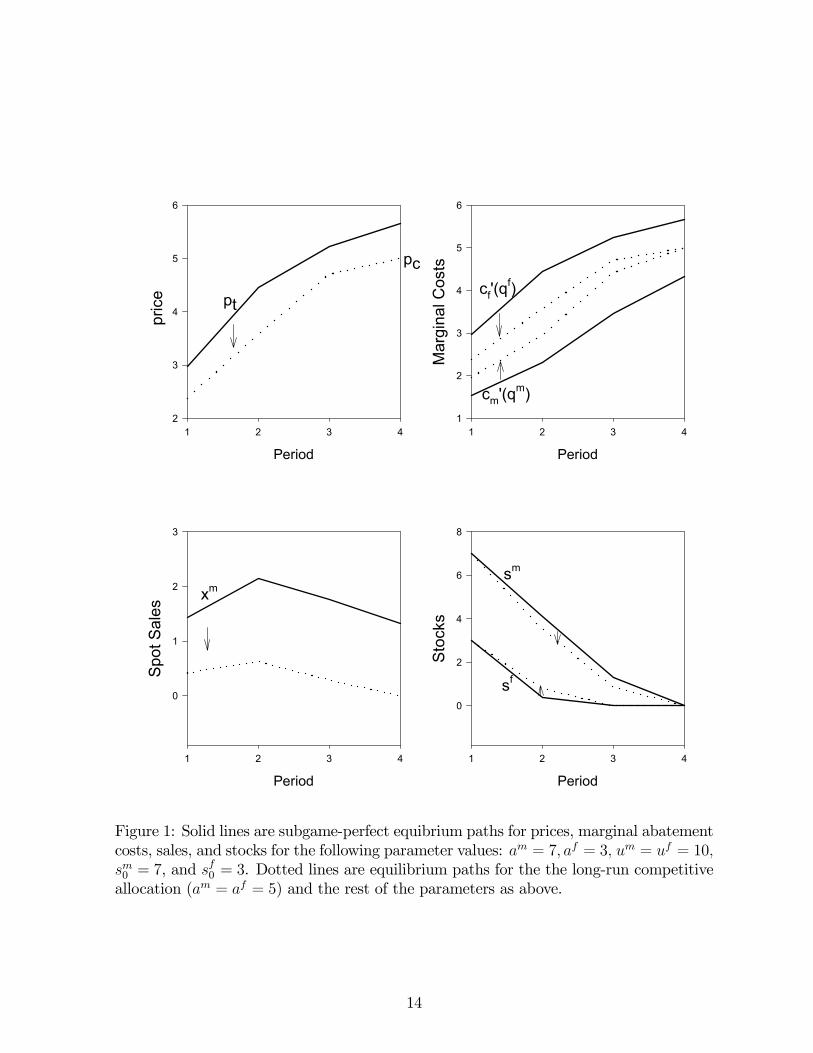
Figure 1 shows the time paths for prices, marginal costs, spot sales, and stocks in two

cases. In the first case, firms are symmetric in all respects but in two: the large firm or

the cartel has a larger flow allocation and a larger share of the initial stock (70% of both

allocations). Note that for this division of stocks, the equilibrium satisfies the restrictions

imposed in our construction (sm3 = sm4 = sf2 = sf3 = sf4 = 0).6 The equilibrium paths are

depicted by the solid lines.

The second case is the same as the first except that the long-run allocation is efficient,

am = a∗, so that there are no distortions in the final stage. The equilibrium paths are

depicted by the dotted lines for this case.

Let us now discuss the qualitative features of the equilibrium paths. The price grows

5If the implicit restrictions on stockholdings are not satisfied, it is not possible to have this charac-terization of equilibrium in four periods. Thus, the equilibrium number of periods depends on the intialstocks, which we have implicitly chosen such that our four period example works.

6In fact, for these parameters, the equilibrium has the depicted qualitative features as long as thelarge firm has more than 38.8% of the initial stock.

12

at the rate of interest between first two periods (1.5p1 = p2) and at a strictly lower rate

between t = 2 and 3, as expected. If am > a∗, the fourth period price is higher than

the competitive price (denoted by pc in the graph), since the allocations imply that the

large firm is the net seller in the absence of permit stocks. If am = af , then the long-run

price is the competitive price, which lowers the price path throughout the equilibrium,

as depicted.

Note that the large firm has a lower marginal cost throughout the banking equilibrium

because it is shifting the abatement burden towards the fringe; the marginal cost of the

latter equals the manipulated price whereas the large firm’s marginal cost equals the

marginal revenue from sales which is lower than the price (which holds for all periods).

The northeastern panel illustrates how the distortion suffered by the fringe’s abatement

efforts during the banking phase decreases when the long-run market power is eliminated.

The sales path xm that keeps the marginal revenue growing at the rate of interest

during banking is first increasing and then declining. When the flow allocation is reduced

to am = a∗, sales during banking go down because the leader has a lower share of the

overall allocation (stock and flow together). Thus, when the long-run equilibrium is

competitive, the leader uses more of the stock for own compliance.

Finally, the last panel shows that the depletion of stocks is faster when the equilibrium

becomes more competitive, i.e., when the leader’s flow allocation is reduced to am = a∗.

Throughout the rest of the paper we use this equilibrium as our benchmark, so it

proves useful to summarize its properties.

Proposition 1 The properties of the manipulated banking path as implied by the bench-

mark model are the following:(i) the competitive stockholdings are exhausted before the

noncompetitive holdings;(ii) prices must ultimately decline in present value (p2(1 + r) >

p3);(iii) the fringe does not equalize present-value marginal costs across all periods whereas

the large firm does; (iv) the long-term market power as identified by Hahn (1984) is ex-

tended to the banking phase.7

7The last point of the proposition has been shown also in Liski and Montero (2004) who consider onlytwo extreme permit allocations.

13

Period

1 2 3 42

3

4

5

6

Period

1 2 3 4M

argi

nal C

osts

1

2

3

4

5

6

Period

1 2 3 4

Sto

cks

0

2

4

6

8

Period

1 2 3 4

Spo

t Sal

es

0

1

2

3

pt

cm'(qm)

cf'(qf)

xm

pric

e

sm

sf

pc

Figure 1: Solid lines are subgame-perfect equibrium paths for prices, marginal abatementcosts, sales, and stocks for the following parameter values: am = 7, af = 3, um = uf = 10,sm0 = 7, and sf0 = 3. Dotted lines are equilibrium paths for the the long-run competitiveallocation (am = af = 5) and the rest of the parameters as above.

14

3 Imperfectly Observed Stockholdings

In permit trading programs the regulator typically runs a computerized "permit (al-

lowance) tracking system" (as in the U.S. Acid Rain program) which together with ac-

curate measuring of emissions makes it easy to monitor the compliance status of the

regulated firms: each firm should have enough permits in its account with the tracking

system to cover its emissions over the compliance period (typically a year). While one

purpose of the tracking system is to provide the information about the compliance of

the regulated firms, a by-product of a transparent tracking system is that the regulated

firms as well as third parties (traders in the permit market) can in principle observe other

traders’ permits in the tracking system. However, in reality, actual permit holdings can

be easily masked by using middlemen such as permit brokers since permit accounts can

be opened not only for the regulated firms but also for outsiders which are nonaffected by

the regulation. Thus, even in the presence of a permit tracking system, it is unreasonable

to think that permit holdings by private entities are fully observed by the market. In

this section we discuss how relaxing full observability of private stockholdings affects the

ability to manipulate the permit banking program.

Let us consider our benchmark model and the example depicted in Figure 1 to il-

lustrate that (i) the equilibrium solution puts an explicit constraint on stockholdings

along the equilibrium path and that (ii) there is a natural tendency to deviate from this

constraint if permit holdings are not observed. In the first period, the fringe is abating

qf1 = 2.972 and buying xm1 = 1.428 units, so the fringe uses u

f −af − qf1 −xm1 = 2.6 units

from its stock (sf0 = 3) in the first period. These numbers are qf2 = 4.458, x

m2 = 2.142,

and uf − af − qf2 − xm2 = 0.4 for period 2. Recall that a requirement of the competitive

phase is that prices grow at the rate of interest, which means that the fringe’s marginal

cost must grow at this rate. Then, we could conjecture that the above equilibrium re-

mains the same if we keep the abatement choices the same (qf1 , qf2 ) = (2.972, 4.458), so

that the marginal costs remain the same, and change the traded quantities such that,

say, xm1 = 1.428 − 0.3 and xm2 = 2.142 + 0.3. This change only makes the fringe to

consume more of its stock in period t = 1 and rely on a larger purchase in period t = 2.

Because the fringe still exhausts its stock in period t = 2 and prices grow at the rate

15

of interest between t = 1 and t = 2, it seems that the change in the traded quantities

can be made without affecting the equilibrium outcome. And if this change is legitimate,

then it seems that the quantities traded between the fringe and the large firm can be

quite arbitrarily chosen, as long as the arbitrage condition on prices and the exhaustion

condition on stocks are satisfied.

However, changing the trading levels as explained above is not consistent with the

requirement that the equilibrium should be subgame perfect: if the large firm’s sales

in the first period are reduced to xm1 = 1.128, then the large firm has a larger and the

fringe has a smaller stock at t = 2 than along the benchmark equilibrium, implying that

the large firm’s choices for abatement and sales, given by qm2 (sm1 , s

f1) and x

m2 (s

m1 , s

f1), will

differ from those chosen along the benchmark path. In fact, this change would imply

that the large firm becomes larger at t = 2 so that it becomes more dominant. If, on the

other hand, we changed the trading pattern such that the fringe buys more at t = 1 and

less at t = 2 from the large firm, then the subgame-perfect equilibrium outcome starting

from t = 2 would become more competitive.

Subgame-perfection thus requires that the stocks (smt , sft ) develop in right proportions

along the equilibrium path which, in turn, fixes a unique trading pattern between the large

firm and fringe. The above-discussed deviations from the equilibrium trading pattern

correspond to the situation where the large firm can make stock purchases or sales at

very lucrative prices. Selling less than xm1 (sm0 , s

f0) in our example implies that the large

firm is effectively buying stocks for the period t = 2 at prices which are lower than the

true equilibrium prices. Selling more than xm1 (sm0 , s

f0) corresponds to the case where the

large firm is able to sell stocks at t = 1 at prices higher than the true equilibrium prices.

Subgame perfection together with the full observability of private permit holdings

puts therefore an explicit constraint on the path for the stockholdings — the large firm

cannot profitably implement a deviation from the subgame-perfect equilibrium stock-

depletion path because the market can fully foresee the changes in subsequent behavior

which, in turn, implies that the current prices will respond in an unfavorable way. It is

important to emphasize that the implications of this model for market power crucially

depend on the fact that market participants can monitor how the stockholdings of the

16

large firm develop. We do not have a model for the situation where private stockholdings

are incompletely observed, but the logic of market manipulation under full observability

suggests that incomplete observability implies a credibility problem for the large firm.

Let us now conclude this section by explaining this credibility problem.

Recall that the permit banking path is manipulated by shifting the large firm’s sales to

later periods (period t = 3 in our benchmark model) such that the present-value prices for

permits ultimately decline, which makes the competitive stockholders willing to exhaust

their stocks during the early periods of the banking phase (periods t = 1, 2 in our model).

As a result, the value of the competitive stockholdings increase, so the fringe is free riding

on the large firm’s market power. Under full observability the large firm has no way of

extracting these free riding rents, but under incomplete observability there is a tendency

to do so. To illustrate this possibility, suppose the market cannot fully observe the

identity of permit suppliers in the permit spot market but, for some reason, still believes

in the benchmark equilibrium path for prices and quantities. In this situation, the market

cannot observe that the large firm is actually saving part of its stock for the monopoly

phase whose existence is necessary for the conjectured prices. In fact, if the market is

believing that the monopoly phase will exist, but cannot observe how the stocks are

depleted, the large firm would have incentives to "hide" behind the fringe and sell more

during the competitive phase in order to take advantage of higher initial prices (recall

that p1 > p3/(1 + r)2). In anticipation of these deviation incentives, the equilibrium

should become more competitive. We leave it open for future research whether this

depletable-stock market can be manipulated at all under incomplete information about

stockholdings.

4 Stock Transactions

Initial permit stocks imply a potentially dramatic increase in the liquidity of the permit

market. There are simply too many permits to be used for compliance in the early periods.

This in turn implies that a market participant can in principle withhold a larger permit

allocation from a spot market than in the long-run when all stocks are exhausted. Since

17

permit stocks typically exist in electronic accounts with zero storage costs, it is natural ask

if these easily movable stocks can be purchased in order to gain market power. Moreover,

because anyone can buy and hold permits, we consider whether the possibility of stock

transactions makes the permit market or its banking phase vulnerable to manipulation

by an outsider who has no initial permit allocation and abatement targets. Stock trading

also raises the possibility that a large firm or cohesive cartel monopolizes the market

further by increasing its share of the overall stock.

Our benchmark model defines the payoffs achievable from holdings (sm0 , sf0) for the

large stockholder and fringe. This Stackelberg game assumes that the holding for the

leader is large enough to justify the ability to move first in each period of the game.

Next we open up the market for stocks such that stocks can be traded before the above

Stackelberg game is played. This allows us to analyze whether a large regulated firm

can improve its leader position in the game or whether an outsider nonaffected by the

regulation can achieve the leader position by buying stocks.

Proposition 2 Given rational expectations and full information, neither a large regu-

lated firm or nonregulated outsider can profitably purchase stocks to gain (further) market

power.

Proof: We consider the regulated firm first since the problem for the outsider follows

as a special case. Let

πm1 (sm0 , s

f0) = xm1 (s

m0 , s

f0)p1(s

m0 , s

f0)− Cm(q

m1 (s

m0 , s

f0)) +

πm2 (sm1 , s

f1)

1 + r

denote the first-period profit defined as a function of initial holdings (sm0 , sf0), as

explained in the analysis of our benchmark model. We are interested in finding out

whether the holdings (sm, sf) = (sm0 , sf0) are in fact the large firm’s preferred holdings

in the presence of a market for stocks. Without losing generality of the argument, we

assume that trading with stocks takes place before the Stackelberg game defining the

payoff πm1 (sm0 , s

f0) is played. The large firm’s problem is to choose a division of stocks to

maxsm[πm1 (s

m, s0 − sm)− p1(sm, s0 − sm) · (sm − sm0 )] (31)

18

given s0 = sm0 + sf0 , where p1 is the rational-expectations price at the first period of the

game starting with the chosen division of stocks, (sm, sf). That is, holding sm can be

increased above sm0 by paying unit price p1 that the market is expecting to prevail when

the Stackelberg game is played. In Appendix B we solve the large firm’s problem in

period t = 1 and show that the shadow value of the fringe stock in equilibrium satisfies

µ =∂

∂sf0πm1 (s

m0 , s

f0) = −xm1 C 00

m(qm1 ) < 0 (32)

The shadow value of the leader’s own stock satisfies

λ =∂

∂sm0πm1 (s

m0 , s

f0) = C 0

f(qf1 )− xm1 C

00m(q

m1 ), (33)

which in equilibrium equals the marginal revenue from sales. The marginal effect of

increasing the large firm’s holding sm through stock trading is

∂

∂smπm1 (s

m, sf)− ∂

∂sfπm1 (s

m, sf)− p1 − ∂

∂smp1 · (sm − sm0 ) =

− ∂

∂smp1 · (sm − sm0 )

which is negative when (sm, sf) = (sm0 , sf0), by (32), (33), and the fact that

∂∂sm

p1 >

0 (making the division of stocks less competitive increases the price level). Thus, a

regulated large firm does not prefer to increase its holdings. In fact, it would prefer to

reduce holdings since adding the stock trading stage to the game is just like adding one

more sales period which, of course, will be used.

The proof for a nonregulated outsider requires the following modifications. First,

(sm0 , sf0) = (0, s0), implying that the banking path is competitive in the absence of any

takeover of the permit bank. Second, the outsider has no abatement target, so qmt = 0 as

well as am = 0. These changes imply that we are left with the Salant’s (1976) description

for market power in a depletable-stock market. Thus, if stock sm > 0 is purchased

and used for market manipulation, then marginal revenues from selling from this stock

satisfies

p1 − xm1 C00f (q

f1 ) =

1

1 + r[p2 − xm2 C

00f (q

f2 )] =

1

1 + r[p3 − xm3 C

00f (q

f3 )]

19

which assumes that sm is sold in three periods. Since the marginal revenue at t = 1

gives the present-value shadow value of having one more unit of sm to be sold in any of

the periods t = 1, 2, 3, it cannot be profitable to buy stocks with price satisfying p1 >

p1 − xm1 C00f (q

f1 ). This reasoning holds irrespective of the number of periods considered.¥

The intuition for the result follows from the observation that the competitive fringe

is free riding on the large stockholder’s market power. Consider the case where the large

stockholder is an outsider who, for some exogenous reason, has stock sm which is sold in

three periods in equilibrium. For the equilibrium to be noncompetitive, the fringe cannot

be selling in the last period. This implies that the last period (t = 3) price is lower in

present value than the first-period price

p1 >p3

(1 + r)2

We observe that it is optimal for the large seller to let the fringe exhaust first and be the

only one selling at t = 3. Although at t = 3 units are sold at a lower price in present

value terms (which explains the fringe’s absence), at the margin the large seller receives

the same revenue for these units that for those sold at t = 1 and 2. Thus, the large

stockholder moves the market by shifting sales to the third period in exchange for an

increase in today’s prices. Of course, the asset values for the fringe increase due to the

presence of the large seller. This is why the fringe is free riding on the large stockholder’s

market power, given the large holding sm. If the large firm does not receive the stock

as an initial allocation, sm = sm0 , it is not profitable to buy this stock from competitive

stockholders: the market price for stocks acquired is the ex-post noncompetitive price

which fully appropriates the gains from market manipulation.

The result has an analog in the shareholder takeover literature (Grossman and Hart

(1980) and, e.g, Holmström and Nalebuff, 1992). An outsider can be interpreted as a

raider making a tender offer for permit stocks. Because in reality permit purchases can

be made during a considerable period of time and stockholdings potentially easily masked

by using middlemen, the takeover may not be fully anticipated and, therefore, the gains

from it may not be fully appropriated by the market. Although our result is limited in

the sense that it depends on the assumption of full information, it is important to observe

20

that an insider (a regulated firm) having long-term market power cannot gain from his

long-term position to increase the noncompetitive stockholding.

5 Forward Trading

Since abatement strategies often involve long-term investments, for example, in energy

production capacity and supply infrastructure and in contracting decisions for inputs

that are complements or substitutes for permits, it is natural to expect a development

of an active futures market for permits. Our prime example, the US market for SO2

emissions, provides salient evidence of such a development in the form of active options,

futures, and "swaps" market (Joskow, Schmalensee, and Bailey, 1998; Ellerman et al.

2000).

While it cannot be directly observed what fraction of the current permit stocks in the

US SO2 program has already been sold in the forward market or otherwise affected by

the futures trading8, our point of departure in this section is the observation that there

exists a futures market for permits and that stocks are actively sold forward.9

In this section our objective is to demonstrate that the typical approach to market

power in a depletable-stock market that we used in our benchmark analysis, is not con-

sistent with an active forward market for permits. In fact, the implications for market

manipulation are critically dependent on the assumption that permit trading is restricted

to spot transactions. While our benchmark model could be extended to the case where

firms in each period t not only sell on the spot market but also trade future delivery

contracts, we do not consider the full subgame-perfect equilibrium for such a game.10

Our purpose is only to demonstrate that forward trading is not in the interests of the

large firm since it necessarily leads to a more competitive outcome.

8The US EPA runs a computerized allowance tracking system that makes current "physical" holdingsof each firm visible to all market participants. However, the system does not reveal whether the currentholding has been sold forward, so in this sense the system does not directly keep track of actual holdings.

9Personal communication with Denny A. Ellerman, MIT Center for Energy and Environmental PolicyResearch.10Allaz and Vila (1993) assume that there is at least one forward sale before the production stage

in a Cournot oligopoly. The same approach could be used here, although our set-up is slightly morecomplicated since there are several "production" stages. For the extension of Allaz and Vila to thisdirection, see Liski and Montero (2004).

21

For this purpose, assume that at t = 1, 2, 3, 4 the timing in the spot market is the same

as previously. That is, the large firm is a Stackelberg leader choosing its abatement and

demand for permits before the fringe. Assume also that at t = 1 there is a forward-market

opening in which market participants can take short and long positions for deliveries in

t = 2. More specifically, a forward contract signed at t = 1 specifies a dated commodity

(permit) that remains in seller’s stock until the date of delivery is reached. The price for

the delivery is made (or formally contracted) at t = 1. Let f i1(2) for i = m, f denote the

quantity of forward sales made at t = 1 for period 2. We assume that participants in the

forward market (other regulated firms, speculators) have rational expectations. There

is also full information about the short positions taken by the stockholders, fm1 (2) and

ff1 (2).11 While we do not explicitly consider the price formation process in the forward

market, forward supplies lead to downward pressure in the forward price and thereby to

speculatory demand; the equilibrium price for forward deliveries will be bid to equal the

expected (discounted) spot price in period t = 2 (see Allaz and Vila, 1993) We assume

that the large firm chooses its forward position first, simultaneously with is abatement

and permit demand decisions.

The expected spot price in period t = 2 and, hence the forward price in period t = 1,

must be obtained by considering whether forward contracting changes the large firm’s

behavior in period t = 2. The relevant question is then the following: do qm2 (sm1 , s

f1) and

xm2 (sm1 , s

f1) obtained for the benchmark model still describe the subgame-perfect strategies

given the holdings (sm1 , sf1), despite the possibility that part of the stocks may have been

already sold before period t = 2 arrives? To test this, note that having contracted fm1 (2)

of its sales for period t = 2 the large firm’s problem is to solve

maxqm2 ,xm2

[p2 · (xm2 − fm1 (2))− Cm(qm2 ) +

πm3 (sm2 )

1 + r]

subject to constraints (15)-(18). Note that xm2 still denotes the overall deliveries in

period 2, so that xm2 − fm1 (2) gives the spot market sales. It is immediately clear that

11This is not entirely realistic assumption because forward positions are typically anonymous. However,relaxing the observability assumption should only strengthen our conclusions since the effect should bepro-competitive, as we will explain below.

22

the large firms marginal revenue from sales in period t = 2,

p2 − (xm2 − fm1 (2)) · C 00f (q

f2 ), (34)

jumps up as a result of forward trading because the revenue from sales fm1 (2) is already

secured. Selling more than xm2 (sm1 , s

f1) in period 2 becomes profitable, leading to more

competitive stock depletion. Because participants in the forward market foresee how

the incentives for spot sales by the large firm are altered by forward contracting, they

rationally expect a forward price that is lower than our benchmark spot price; the price

is lower, the greater the quantity of sales contracted forward by the large firm.

The above reasoning shows, without specifying what determines the demand for for-

ward contracting, that the large firm cannot make forward sales without reducing its

payoff. One might argue that selling the entire stockholding forward would avoid the

problem because, if the large firm has no "uncommitted" stock left, it cannot flood the

spot market with additional supplies. To test this argument, we would have to allow for

additional forward market openings. Suppose that the forward market at t = 1 allows

forward sales to periods t = 2, 3, and at t = 2 to period t = 3. Assume then that the

first forward position for the large firm is "full" in the sense that

fm1 (2) + fm1 (3) = sm0 − xm1 .

That is, the stock remaining after the first spot sale is fully offered to the forward market.

Suppose that this forward trading strategy solves the large firm’s credibility problem

discussed above. Then, given this conjecture, our benchmark spot prices identify the

forward prices with which the large firm can make the forward sales. However, these

prices are declining in present value after period 2 (see (30)), which creates an arbitrage

opportunity for the large firm: the firm can buy back its deliveries for period t = 3 to

make additional sales in period t = 2.

The arbitrage can be implemented as follows. When period 2 forward market opens,

the large firm takes a long position for deliveries in t = 3. This reduces the large firm’s

delivery commitments to period t = 3 below the original forward sales fm1 (3), making

23

it possible to sell more in spot market t = 2 (recall that the firm is still holding the

stocks from which the commitments to period t = 3 were made). This deviation from

the original plan implies a reduction in the spot price below the conjectured spot price

at t = 2 and losses on those who bought delivery contracts fm1 (2) at the conjectured

price. Thus, the conjectured price path cannot be an equilibrium path. In fact, when the

large firm sells the entire stockholding forward, the equilibrium price path must have a

competitive shape: if prices are declining in present value terms, which is a property of a

noncompetitive price path, then the above discussed arbitrage opportunities must exist.

We can now summarize these findings.

Proposition 3 Forward-market opening does not change the large firm’s sales behavior.

That is, in subgame-perfect equilibrium all sales are made in the spot market.

Proof: Follows from the discussion above.¥The result implies that if we observe extensive forward trading by the "suspected"

market participant, then this participant should not be involved in market manipulation.

In other words, because the large firm can commit to its original marginal revenue from

permit sales and, thereby, to its maximum profits by avoiding forward sales, we should

not observe forward trading by the large firm. There are, of course, limitations to this

argument. First, there might be hedging or other reasons for the existence of a demand

for forwards, so the large firm may want to sacrifice part of its market power to satisfy

this demand. Second, if forward positions are anonymous in the sense that the market

observes only the aggregate forward position, the large firm may not be able to commu-

nicate to the market that it has not altered the position of its marginal revenue curve by

making forward sales. We do not have a model for this incomplete information situation

but suspect that the equilibrium outcome must become more competitive due to the lack

of information regarding the identity of sellers in the forward market.12

12If observability is limited, there is always a possibility that the large firm serves a spot market manytimes, which implies losses on contract holders unless prices are adjusted downwards at the outset totake the deviation possiblities into account.

24

6 Conclusions

We have investigated the effect of market power on the equilibrium path of an emission

permit market in which firms bank current permits for gradual use in later periods. In

particular, we have studied the equilibrium for a large (potentially dominant) firm and

a competitive fringe with rational expectations. When permit trading is limited to spot

transactions, we characterized a subgame-perfect equilibrium in which the large firm can

credibly manipulate the permit banking program. The results imply that the ability to

move the banking path depends not only on the size of the stockholding but also on

the long-run market power depending on long-run allocations. This property makes the

intertemporal permit market different from previously analyzed depletable-stock markets.

Using the above benchmark equilibrium we considered how the ability to manipulate

the permit banking program is affected by three changes in assumptions that reflect im-

portant features of existing permit trading programs. First, we found that trading with

permit stocks does not make the permit market more vulnerable to manipulation. Sec-

ond, an active forward market implies that the full gains from market power achievable

under pure spot transactions cannot exist. Third, imperfectly observed permit holdings

imply a potential credibility problem for the large firm, making the market again more

competitive, as compared to the benchmark outcome. Thus, all these "real world" ob-

servations have pro-competitive implications, leading us to conclude that manipulating

a permit banking program may be a very difficult undertaking even for a large permit

stockholder.

7 Appendix A

Taking sf1 and sm1 as given, the large firm solves (14) subject to (15)–(18). Replacing

p2 = C 0f(q

f2 ) into the objective function, the first order conditions for q

m2 and xm2 are,

respectively (recall that sf2 = 0 by assumption)

xm2 C00f (q

f2 )∂qf2 (q

m2 , x

m2 )

∂qm2− C 0

m(qm2 ) +

1

1 + r

dπm3 (sm2 (q

m2 , x

m2 ))

dsm2

∂sm2∂qm2

= 0 (35)

25

C 0f(q

f2 ) + xm2 C

00f (q

f2 )∂qf2 (q

m2 , x

m2 )

∂xm2+

1

1 + r

dπm3 (sm2 (q

m2 , x

m2 ))

dsm2

∂sm2∂xm2

= 0 (36)

From (17) and (18) we know that qf2 (qm2 , x

m2 ) = −xm2 +uf − af − sf1 , so ∂q

f2/∂q

m2 = 0 and

∂qf2/∂qm2 = −1. Similarly, (16) gives the expression for sm2 (qm2 , xm2 ), so ∂sm2 /∂qm2 = 1 and

∂sm2 /∂xm2 = −1.

To obtain dπm3 (sm2 )/ds

m2 , let us rewrite (13) as

πm3 (qm3 (s

m2 ), s

m2 ) ≡ πm3 (s

m2 ) = xm3 (q

m3 , s

m2 ) · C 0

f(qf3 (q

m3 , s

m2 ))− Cm(q

m3 )

where qm3 (sm2 ) is the solution to (7) for any given sm2 . Then, from the envelope theorem

we havedπm3 (s

m2 )

dsm2=

∂xm3∂sm2

C 0f(·) + xm3 · C 00

f (·)∂qf3∂sm2

(37)

And since ∂xm3 /∂sm2 = 1 from (9) and ∂qf3/∂s

m2 = −1 from the combination of (9), (9)

and sf2 = 0, eq. (37) becomes dπm3 (s

m2 )/ds

m2 = C 0

f(qf3 )−xm3 C 00

f (qf3 ). In addition, using the

first order condition (12), yields

dπm3 (sm2 )

dsm2= C 0

m(qm3 ) (38)

Finally, replacing (38) and the above partial derivatives into (35) and (36), the first order

conditions reduce to (19) and (20) in the text.

8 Appendix B

Taking sm0 and sf0 as given, the large firm must solve (22) subject to (23)–(27). Using

(26) and (27), we can rewrite the large firm’s optimization problem as

maxqm1 ,xm1 ,sm1 ,sf1 ,q

f1

xm1p2(s

m1 , s

f1)

1 + r− Cm(q

m1 ) +

πm2 (sm1 , s

f1)

1 + r(39)

subject to (24), (25) and p2(sm1 , sf1)/(1+r) = C 0

f(qf1 ). Letting λ, µ and ξ be, respectively,

the Lagrangian multipliers associated to these three constraints, the first order conditions

26

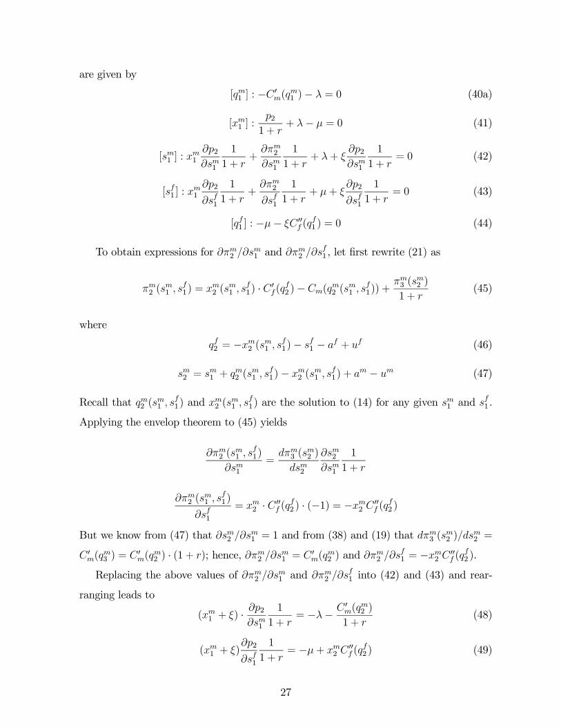
are given by

[qm1 ] : −C 0m(q

m1 )− λ = 0 (40a)

[xm1 ] :p21 + r

+ λ− µ = 0 (41)

[sm1 ] : xm1

∂p2∂sm1

1

1 + r+

∂πm2∂sm1

1

1 + r+ λ+ ξ

∂p2∂sm1

1

1 + r= 0 (42)

[sf1 ] : xm1

∂p2

∂sf1

1

1 + r+

∂πm2∂sf1

1

1 + r+ µ+ ξ

∂p2

∂sf1

1

1 + r= 0 (43)

[qf1 ] : −µ− ξC 00f (q

f1 ) = 0 (44)

To obtain expressions for ∂πm2 /∂sm1 and ∂πm2 /∂s

f1 , let first rewrite (21) as

πm2 (sm1 , s

f1) = xm2 (s

m1 , s

f1) · C 0

f(qf2 )− Cm(q

m2 (s

m1 , s

f1)) +

πm3 (sm2 )

1 + r(45)

where

qf2 = −xm2 (sm1 , sf1)− sf1 − af + uf (46)

sm2 = sm1 + qm2 (sm1 , s

f1)− xm2 (s

m1 , s

f1) + am − um (47)

Recall that qm2 (sm1 , s

f1) and xm2 (s

m1 , s

f1) are the solution to (14) for any given sm1 and sf1 .

Applying the envelop theorem to (45) yields

∂πm2 (sm1 , s

f1)

∂sm1=

dπm3 (sm2 )

dsm2

∂sm2∂sm1

1

1 + r

∂πm2 (sm1 , s

f1)

∂sf1= xm2 · C 00

f (qf2 ) · (−1) = −xm2 C 00

f (qf2 )

But we know from (47) that ∂sm2 /∂sm1 = 1 and from (38) and (19) that dπm3 (s

m2 )/ds

m2 =

C 0m(q

m3 ) = C 0

m(qm2 ) · (1 + r); hence, ∂πm2 /∂s

m1 = C 0

m(qm2 ) and ∂πm2 /∂s

f1 = −xm2 C 00

f (qf2 ).

Replacing the above values of ∂πm2 /∂sm1 and ∂πm2 /∂s

f1 into (42) and (43) and rear-

ranging leads to

(xm1 + ξ) · ∂p2∂sm1

1

1 + r= −λ− C 0

m(qm2 )

1 + r(48)

(xm1 + ξ)∂p2

∂sf1

1

1 + r= −µ+ xm2 C

00f (q

f2 ) (49)

27

Furthermore, from (40a) and (41) we can express λ and µ as functions of the control

variables and from (19) and (20) we know that p2 − xm2 · C 00f (q

f2 ) = C 0

m(qm2 ). Replacing

these expressions into (48) and (49) yields

(xm1 + ξ) · ∂p2∂sm1

1

1 + r= C 0

m(qm1 )−

C 0m(q

m2 )

1 + r(50)

(xm1 + ξ)∂p2

∂sf1

1

1 + r= C 0

m(qm1 )−

C 0m(q

m2 )

1 + r(51)

Since an increase in stock holdings necessarily leads to more a competitive outcome, we

must have that both ∂p2/∂sm1 and ∂p2/sf1 are strictly negative. Similarly, since a transfer

of a marginal fraction of stock from competitive hands (i.e., fringe) to an strategic player

(i.e., large firm) necessarily leads to a less competitive outcome (unless firms are following

competitive pricing), we must also have ∂p2/∂sf1 < ∂p2/∂s

m1 . Without explicitly solving

for ∂p2/∂sm1 and ∂p2/sf1 ,13 these two observations are sufficient to infer that the only

solution of the system (50)—(51) must satisfy xm1 +ξ = 0 and C0m(q

m1 )−C 0

m(qm2 )/(1+r) = 0.

The latter expression is (28) in the text. To obtain (29), simply replace ξ = −xm1 into(44), and that along with p2/(1 + r) = p1 and λ = −C 0

m(qm1 ) into (41).

References

[1] Allaz, B., and J.-L.Vila (1993), Cournot competition, forward markets and efficiency,

Journal of Economic Theory 59, 1-16.

[2] Bernard, A., S. Paltsev, J.M. Reilly, M. Vielle and L. Viguier (2003), Russia’s role

in the Kyoto Protocol, Report No. 98, Joint Program on the Science of Policy and

Global Change, MIT.

13If we consider, as we do in the numerical examples, that Cf (qf ) = (qf )2/2 and Cm(q

m) = γ(qm)2/2,where γ is some positive parameter, we have that

∂p2∂sm1

= −κ and∂p2

∂sf1=−(κ+ 1)

2

where κ = γ/[(2 + r)(2 + γ)] < 1.

28

[3] Cronshaw, M. and J.B. Kruse (1996), Regulated firms in pollution permit markets

with banking, Journal of Regulatory Economics 9, 179-189.

[4] Ellerman, A.D, P. Joskow, R. Schmalensee, J.-P. Montero, and E.M. Bailey (2000),

Markets for Clean Air: The US Acid Rain Program, Cambridge University Press,

Cambridge, UK.

[5] Ellerman, A.D., and J.-P. Montero (2005), The efficiency and robustness of allowance

banking in the U.S. Acid Rain Program, mimeo, MIT-CEEPR.

[6] Ellerman, A.D., and I. S. Wing (2000), Supplementarity: An Invitation to Monop-

sony? The Energy Journal 21, 29-59.

[7] Hahn, R. (1984), Market power and transferable property rights, Quarterly Journal

of Economics 99, 753-765.

[8] Hagem, C., and H. Westskog (1998), The design of a dynamic tradable quota system

under market imperfections, Journal of Environmental Economics and Management,

36, 89-107.

[9] Hotelling, H. (1931), The economics of exhaustible resources, Journal of Political

Economy 39, 137-175.

[10] Holmström Bengt, and Barry Nalebuff, To the Raider Goes the Surplus? A Reexam-

ination of the Free-Rider Problem, Journal of Economics and Management Strategy

1, 37-62 (1992).

[11] Grossman, Sanford J., and Oliver D. Hart (1980), Takeover Bids, the Free-Rider

Problem, and the Theory of the Corporation, Bell Journal of Economics 11, 42-64 .

[12] Joskow, P., R. Schmalensee, E. Bailey (1998), The Market for Sulfur Dioxide Emis-

sions, American Economic Review, 88, 669-85.

[13] Lewis, T. and R.Schmalensee (1980), On oligopolistic markets for nonrenewable

resources, Quarterly Journal of Economics 95, 475-491.

29

[14] Liski M., and J.-P. Montero (2004), A Note on Market Power in an Emission Permits

Market with Banking, WP-2004-05, MIT-CEEPR.

[15] Liski M., and J.-P. Montero (2004), Forward Trading and Collusion in Oligopoly,

WP-2004-012, MIT-CEEPR.

[16] Maeda, A. (2003), The emergence of market power in emission rights markets: The

role of the initial permit distribution, Journal of Regulatory Economics 24, 293-314.

[17] Newbery, D.M. (1981), Oil prices, cartels and the problem of dynamic inconsistency,

Economic Journal 91, 617-646.

[18] Rubin, J.D. (1996), A model of intertemporal emission trading, banking, and bor-

rowing, Journal of Environmental Economics and Management 31, 269-286.

[19] Salant, S.W. (1976), Exhaustible resources and industrial structure: A Nash-

Cournot approach to the world oil market, Journal of Political Economy 84, 1079-

1093.

[20] Schennach, S.M. (2000), The economics of pollution permit banking in the con-

text of Title IV of the 1990 Clean Air Act Amendments, Journal of Environmental

Economics and Management 40, 189-210.

30