On Kendall's Process

File: 683J 161201 . By:CV . Date:21:08:96 . Time:14:54 LOP8M. V8.0. Page 01:01Codes: 4414 Signs: 1960 . Length: 50 pic 3 pts, 212 mm

Journal of Multivariate Analysis � MV1612

journal of multivariate analysis 58, 197�229 (1996)

On Kendall's Process

Philippe Barbe

C.N.R.S., Universite� Paul-Sabatier, Toulouse Cedex, France

Christian Genest

Universite� Laval, Sainte-Foy, Que� bec, Canada

and

Kilani Ghoudi and Bruno Re� millard

Universite� du Que� bec a� Trois-Rivie� res, Trois-Rivie� res, Que� bec, Canada

Let Z1 , ..., Zn be a random sample of size n�2 from a d-variate continuousdistribution function H, and let Vi, n stand for the proportion of observations Zj ,j{i, such that Zj�Zi componentwise. The purpose of this paper is to examinethe limiting behavior of the empirical distribution function Kn derived from the(dependent) pseudo-observations Vi, n . This random quantity is a natural non-parametric estimator of K, the distribution function of the random variableV=H(Z ), whose expectation is an affine transformation of the population versionof Kendall's tau in the case d=2. Since the sample version of { is related in thesame way to the mean of Kn , Genest and Rivest (1993, J. Amer. Statist. Assoc.)suggested that - n[Kn(t)&K(t)] be referred to as Kendall's process. Weakregularity conditions on K and H are found under which this centered process isasymptotically Gaussian, and an explicit expression for its limiting covariance func-tion is given. These conditions, which are fairly easy to check, are seen to apply tolarge classes of multivariate distributions. � 1996 Academic Press, Inc.

1. INTRODUCTION

Let Z1 , ..., Zn be a random sample of size n�2 from a continuous multi-variate distribution H(z)=P(Z�z) with marginals F1 , ..., Fd , and let Vi, n

article no. 0048

1970047-259X�96 �18.00

Copyright � 1996 by Academic Press, Inc.All rights of reproduction in any form reserved.

Received August 23, 1995; revised March 1996.

AMS 1990 subject classifications; 60F05, 62E20.Key words and phrases: asymptotic calculations, copulas, dependent observations, empiri-

cal processes, Vapnik�C2 ervonenkis classes.


stand for the proportion of observations Zj , j{i, such that Zj�Zi com-ponentwise, namely

Vi, n=*[ j{i : Zj�Zi]�(n&1).

Let also Kn be the empirical distribution function based on the Vi, n 's andK be the distribution function of the random variable V=H(Z ) takingvalues in [0, 1].

The purpose of this paper is to examine the limiting behavior of theempirical process

:n(t)=- n[Kn(t)&K(t)],

taking values in the space D of ca� dla� g functions from [0, 1] to R. Genestand Rivest (1993), who originally defined :n in the restricted case where His bivariate, proposed to call it Kendall's process. This terminology isjustified by the fact that the empirical and population values {n and { ofKendall's tau are affine transformations of the means of distribution func-tions Kn and K, respectively. As the relations

|1

0t dK(t)=E(V )=

2d&1&12d ({+1)

and

|1

0t dKn=

1n

:n

i=1

Vi, n=V� =2d&1&1

2d ({n+1)

define natural extensions of Kendall's measure of association in arbitrarydimension d�2 (Joe, 1990), the terminology remains appropriate even inthat case.

What will be shown here is that under fairly weak regularity conditions,:n converges in distribution to a continuous, centered Gaussian process :.This result and the techniques used to obtain it are of interest on variousaccounts. The chief theoretical reason is that the empirical distribution Kn

is constructed from pseudo-observations Vi, n whose dependence structureis not amenable to standard tightness techniques. Thus the argumentspresented herein are archetypical of the approach required to study theasymptotic behavior of empirical processes derived from U-statistics suchas Kendall's tau. From a practical angle, this paper's main result hasbearing on the elaboration of confidence regions and goodness-of-fit proce-dures with overall confidence level based on the estimation Kn of K. Ashighlighted by Genest and Rivest (1993), there are families of multidimen-sional distributions whose dependence structure is characterized by the

198 BARBE ET AL.

kghoudi

Comment on Text

remove bracket

kghoudi

Highlight

kghoudi

Highlight

kghoudi

Highlight


univariate function K. On a more prospective note, the connection betweenthe latter quantity and Kendall's tau suggests that new, useful measuresand concepts of dependence could be defined in terms of K. The large-sample properties of Kn would then come in handy in the developmentof statistical inference procedures for testing against these varieties ofdependence.

Exact conditions under which Kendall's process converges weakly arestated in Section 2, together with an explicit expression for the covariancefunction of its limit :. This section also provides alternative regularityconditions that facilitate the verification of the hypotheses of the maintheorem. Section 3 presents a number of well-known families of distribu-tions to which these conditions apply. A sketch of the proof of the mainresult is then given in Section 4. The details of the argument can be foundin Sections 5 and 6. Section 7 proves that the alternative regularity condi-tions given in Section 2 are sufficient.

2. STATEMENT OF THE MAIN RESULTS

Let Z1 , ..., Zn be n�2 independent copies of a vector Z=(Z (1), ..., Z (d ))with continuous distribution function H(z) and marginals F1 , ..., Fd , and let

Vi, n=*[ j{i : Zj�Zi]�(n&1).

Denote by Kn the empirical distribution function of the Vi, n's and let K bethe distribution function of the random variable V=H(Z ) taking values in[0, 1]. In order to establish the weak convergence of the process:n(t)=- n[Kn(t)&K(t)], the following assumptions will be made on thedistribution functions K and H. Note that the second hypothesis is in facta condition on the (unique) function H� associated to H through therelation H(z)=H� [F1(z(1)), ..., Fd (z(d ))]. In the terminology of Sklar (1959),H� is a copula, that is, a distribution function on [0, 1]d with uniformmarginals.

Hypothesis I. The distribution function K(t) of V=H(Z ) admits acontinuous density k(t) on (0, 1] that verifies k(t)=o[t&1�2 log&1�2&=(1�t)]for some =>0 as t � 0.

Hypothesis II. There exists a version of the conditional distribution ofthe vector (F1(Z (1)), ..., Fd (Z (d ))) given H(Z )=t and a countable family Pof partitions C of [0, 1]d into a finite number of Borel sets satisfying

infC # P

maxC # C

diam(C )=0,

199ON KENDALL'S PROCESS


such that for all C # C, the mapping

t [ +t(C)=k(t) P[(F1(Z (1)), ..., Fd (Z (d ))) # C | H(Z )=t]

is continuous on (0, 1] with +1(C )=k(1) I[(1, ..., 1) # C].Given 0�s, t�1, define

Q(s, t)=P[H(Z1)�s, Z1�Z2 | H(Z2)=t]&tK(s)

and

R(s, t)=P[Z1�Z2 7 Z3 | H(Z2)=s, H(Z3)=t]&st,

where u 7 v denotes the componentwise minimum between u and v.

With this notation, the main result to be proved here may now be statedprecisely as follows. For a strengthened version of Hypothesis II that iseasier to verify, the reader may refer to Theorem 2.

Theorem 1. Under Hypotheses I and II above, the empirical process :n

converges in distribution to a Gaussian process : with zero mean andcovariance function

1(s, t)=K(s 7 t)&K(s) K(t)+k(s) k(t) R(s, t)&k(t) Q(s, t)&k(s) Q(t, s).

In particular, Q(t, t)=t[1&K(t)] and hence

1(t, t)=K(t)[1&K(t)]+k(t)[k(t) R(t, t)&2t[1&K(t)]],

in accordance with the expression given by Genest and Rivest (1993).

In view of the fact that - n({n&{) can be expressed as a linear functionalof :n through the relation

- n({n&{)=&\ 2d

2d&1&1+ |1

0:n(t) dt,

an immediate by-product of the above theorem is that this quantity convergesweakly to a centered Gaussian random variable with variance given by

\ 2d

2d&1&1+2

|1

0|

1

01(s, t) ds dt=\ 2d

2d&1&1+2

var[H(Z)+H� (Z )],

where H� (z)=P(Z>z). For additional material on the limiting behavior of- n {n and other U-statistics, the reader may refer to the excellentmonograph by Lee (1985).

To simplify the application of Theorem 1, an alternative condition thatimplies Hypothesis II is identified next. To this end, let ?i (z) be the

200 BARBE ET AL.


projection of z # [0, 1]d onto the (d&1)-dimensional subspace obtained byomitting component z(i ). Let also H be the class of copulas having acontinuous density on (0, 1)d and such that there exists 1�i�d so that forany x # [0, 1]d&1 satisfying P[?i(Z)�x]>0, the conditional distributionfunction

Hi ( y | x)=P[Z (i)� y | ?i (Z)�x], 0� y�1,

verifies �Hi ( y | x)��y>0 on the set [ y : 0<Hi ( y | x)<1].To be specific, let H # H be a fixed copula with continuous density h.

Without loss of generality, one may assume that

��y

Hd ( y | x)=1

H(x, 1)�

�yH(x, y)>0

whenever H(x, 1)>0 and 0<Hd ( y | x)<1. Define

Qx(t)=inf[ y # [0, 1] : Hd ( y | x)�t],

the left-continuous quantile function associated to the conditional distribu-tion of Z (d ) given ?d (Z)�x. For the sake of simplicity, let also

ht(x)=_ ddt

Qx[t�H(x, 1)]& h _x, Qx[t�H(x, 1)]&_I[x # (0, 1)d&1 : H(x, 1)>t],

where the existence and continuity of dQx(t)�dt are guaranteed by theInverse Function Theorem (Theorem 9.24 in Rudin, 1976).

The following result shows that Hypothesis II is automatically verifiedfor all copulas in class H and, in particular, for all copulas whose densityfunction is continuous and strictly positive on (0, 1)d.

Theorem 2. Suppose that H is a copula belonging to class H. Thenthere exists a version of the conditional distribution of Z given H(Z)=tsuch that for any rectangle C in [0, 1]d, the mapping t [ +t(C )=k(t) P[Z # C | H(Z )=t] is continuous on (0, 1] and +1 is the Dirac measurewith mass k(1) at point (1, ..., 1). Moreover, for any Borel set C in [0, 1]d

and for any 0<t<1, +t(C ) admits the representation

+t(C )=|(0, 1)d&1

I[(x, Qx[t�H(x, 1)]) # C] ht(x) dx.

In particular, k(t)=� (0, 1)d&1 ht(x) dx.

The proof of this theorem is given in Section 7.



3. EXAMPLES OF APPLICATION

This section records a few examples of classical families of copulas forwhich Kendall's process converges. While the list is by no meansexhaustive, it is sufficiently long to indicate that Hypotheses I and II arenot unduely restrictive.

Example 1. The simplest test case is provided by the independencecopula H(z)=>d

i=1 z(i ). Since its density is one on (0, 1)d, it is plain thatH belongs to class H. In addition,

&log[H(Z )]=& :d

i=1

log[Z (i )]

has a gamma distribution with parameters :=d and ;=1, from which itfollows that k(t)=logd&1(1�t)�(d&1)!=o[t&1�2 log&1�2&=(1�t)] as t � 0for any =>0. It is easy to check that

K(t)=t :d&1

i=0

logi(1�t)i !

.

Lengthy but straightforward calculations yield

Q(s, t)=(s 7 t) :d&1

i=0

logi(t�s 7 t)i !

&tK(s).

It will also follow from a more general formula derived in Example 3 that

R(s, t)=E _exp _ :d

i=1

min[log(s) U (i )1 , log(t) U (i )

2 ]&& ,

where U1 and U2 are independent copies of a random vector uniformly dis-tributed on the simplex in [0, 1]d. This leads to a cumbersome but explicitexpression for the covariance function 1(s, t), which reduces to

1(s, t)=st&(s 7 t)[1+log(s 6 t)]

when d=2. Here, u 6 v stands for the maximum between u and v.

Example 2. It is not necessary to be able to compute k(t) explicitly toverify that it has the appropriate behavior in the neighborhood of theorigin. To illustrate this point, consider the bivariate Farlie�Gumbel�Morgenstern class of distributions, which is often used in practice to modelsmall departures from independence (for a recent application, see, for

202 BARBE ET AL.


example, de la Horra and Fernandez, 1995). Its associated copula is ofthe form H(x, y)=xy+%xy(1&x)(1& y) with |%|�1. Since h(x, y)=1+%(1&2x)(1&2y) is strictly positive on (0, 1)2, it is clear that H # H.Setting cx=%(1&x) and

rx=rx(t)=- (1&cx)2+4cx(1&t�x)=- (1+cx)2&4cxt�x�x,

one finds successively

Qx(t)={t if cx=0

1+cx&rx(tx)2cx

if cx{0

and

ht(x)=h[x, Qx(t�x)]

xrx(t)I(1�x>t)

=x(1&rx)+(1&x) rx

x(1&x) rxI(1�x>t)

={ 1&rx

(1&x) rx+

1x= I(1�x>t)

={ 1&r2x

(1&x) rx (1+rx)+

1x= I(1�x>t)

�1+2 |%|

xI(1�x>t),

the last inequality holding true because 1&r2x�2 |%|(1&x). While a simple

algebraic form does not exist for

k(t)=|1

tht(x) dx,

it is plain that

k(t)�(1+2 |%| ) log(1�t)

for all |% | � 1. Consequently, k(t) = o[t&1�2 log&1�2&=(1�t)] for all&1�%�1 and arbitrary =>0, which implies that the associated Kendallprocess converges asymptotically. It does not seem possible to derive anexplicit algebraic expression for the covariance 1(s, t) of the limitingKendall process associated to this family of copulas.



Example 3. Archimedean copulas (Genest 6 MacKay, 1986a, b) forma general class of multivariate dependence functions that includes inde-pendence (,(t)=log(1�t)) and many well-known parametric systems ofdistributions, including those proposed by Ali, Mikhail 6 Haq (1978),Clayton (1978), Frank (1979), and Gumbel (1960). In the simplest of cases,these copulas are expressed as

H(z)=,&1 _ :d

i=1

,[z(i )]&in terms of a bijective generator , from (0, 1] into [0, �) satisfying(&1) i d i,&1(t)�dti>0 for 1�i�d and ,(1)=0.

Put x=(z(1), ..., z(d&1)) and y=z(d ) and observe that

��y

H(x, y)=,$( y)

,$[H(x, y)]>0

for all 0< y<1 whenever 0<H(x, y)<1. It is thus clear that all copulasof this form belong to class H. To check whether they meet Hypothesis I,first introduce f0(t)=1�,$(t) and for i�1, define fi (t) recursively throughthe formula fi (t)= f $i&1(t)�,$(t). It is straightforward to see that

fi (t)=d i+1

dsi+1 ,&1 } s=,(t)

and that

�i+1

�xi } } } �x1 �yH(x, y)=,$( y) ,$[x(1)] } } } ,$[x(i )] fi [H(x, y)],

so that

h(x, y)=,$( y) ,$[x(1)] } } } ,$[x(d&1)] fd&1[H(x, y)]

for all x # (0, 1)d&1 and 0<y<1.Recalling that H[x, Qx[t�H(x, 1)]]=t by definition, one finds

��t

Qx { tH(x, 1)==

,$(t),$[Qx[t�H(x, 1)]]

,

from which it follows that

ht(x)=(&1)d&1

(d&1)!,d&1(t) ,$(t) fd&1(t)

_{(d&1)! _ `d&1

i=1

&,$[x(i )],(t) & I _ :

d&1

i=1

,[x (i )],(t)

<1&= .

204 BARBE ET AL.


Summing over all values of x # (0, 1)d&1 and using the fact that the termin braces integrates to one on this domain, one may conclude that

k(t)=|(0, 1)d&1

ht(x) dx=(&1)d&1 ,d&1(t) ,$(t) fd&1(t)�(d&1)!

It is then a routine exercise to check that

K(t)=t+ :d&1

i=1

(&1) i ,i(t)i !

fi&1(t),

provided that limt � 0+ ,i(t) fi&1(t)=0 for all 1�i�d&1.Note in passing that the above expression for ht(x) also suggests the

following extension of Proposition 1.1 in Genest and Rivest (1993).

Theorem 3. Let U # [0, 1]d be a d-dimensional random vector uniformlydistributed over the simplex [z # [0, 1]d : �d

i=1 z(i )=1], and let V be a ran-dom variable with density

k(v)=(&1)d&1 ,d&1(v) ,$(v) fd&1(v)�(d&1)!

defined in terms of the generator , of multivariate Archimedean copula H. IfU and V are independent, then H is the distribution function of the vector Zwith components Z (i )=,&1[U (i ),(V )], 1�i�d.

Proof. Let Z$ be an observation from distribution H and f be a con-tinuous function on [0, 1]d. What needs to be shown is that E[ f (Z$)]=E[ f (Z )]. To this end, simply write

E[ f (Z$)]=|1

0k(v) E[ f (Z$) | H(Z$)=v] dv

=|1

0|

(0, 1)d&1f _x, Qx { v

H(x, 1)=& hv(x) dx dv

and make the change of variables x(i )=,&1[u(i ),(v)] for 1�i�d&1 withu(d )=1&�d&1

i=1 u(i ), so that

du=_ `d&1

i=1

&,$[x(i )],(t) & dx.



An alternative expression for E[ f (Z$)] is thus given by

(d&1)! |1

0|

(0, 1)d&1k(v) f [,&1[u(1),(v)], ..., ,&1[u(d ),(v)]]

_I { :d&1

i=1

u(i )<1= du dv,

which is nothing but E[ f (Z )]. Hence the proof is complete. K

Among families of Archimedean copulas whose corresponding k(t)satisfies Hypothesis I for any d�2, one may mention:

(i) Clayton's family of copulas, whose generator is ,%(t)=(t&%&1)�% for %�0. In this case,

fi (t)=(&1) i+1 t1+(i+1) % `i

j=0

(1+ j%), i�0

and

k(t)={ `d&1

i=1

(1+i%)= \1&t%

% +d&1

<(d&1)!,

which is o[t&1�2 log&1�2&=(1�t)] for any =>0. Independence, which wastreated in Example 1, corresponds to the limiting case %=0.

(ii) Frank's family of copulas (Nelsen, 1986; Genest, 1987), whosegenerator is

,%(t)=&log \1&%t

1&% +with 0<%<�. In this case,

fi (t)=pi (%&t)�log(%), i�0

and

k(t)=pd&1(%&t)

(d&1)! (%&t&1) {log \1&%t

1&%+=d&1

=&%&tp$d&2(%&t)

(d&1)! {log \1&%t

1&% +=d&1

,

206 BARBE ET AL.


where p0(x)=x&1 and pi (x) is defined recursively by the formulapi (x)=x(1&x) p$i&1(x) for arbitrary i�1. Therefore,

k(t)tlogd&1(1�t)�(d&1)!

as t � 0, so that Hypothesis I is again satisfied for any =>0.

(iii) Gumbel's family of copulas, whose generator is ,%(t)=log1�%(1�t)for 0<%�1. In this case,

fi (t)=(&1) i+1 %t log1&(i+1)�% (1�t) pi[log(1�t)], i�0

and

k(t)= pd&1[log(1�t)]�(d&1)!,

where p0(x)=1, and pi (x)=%x[ pi&1(x)&p$i&1(x)]+(1+i&%) pi&1(x),i�1. Since pd&1 is a polynomial of degree d&1 with leading coefficient%d&1, it follows that k(t)t(%d&1�(d&1)!) logd&1(1�t) as t � 0, whenceHypothesis I is verified.

(iv) Ali, Mikhail and Haq's family of copulas, whose generator is

,(t)=1

1&%log \1&%+%t

t +for 0<%�1. In this case, f0(t)=&t(1&%+%t), fi is a polynomial in t suchthat fi (0)=0 and f i$(0)=(&1)i+1 (1&%) i+1, i�0. It follows thatk(t)tlogd&1(1�t)�(d&1)! as t � 0, whence Hypothesis I is verified.

Finally, using Theorem 3, it is possible to derive the following expres-sions for the functions Q(s, t) and R(s, t) required to compute the limitingcovariance function of Kendall's process, when the underlying copula is ofthe Archimedean variety. Indeed, if Z1 , Z2 are independent random vectorswith copula H(z)=,&1[�d

i=1 ,[z(i )]], and if U1 , U2 , V1 , V2 are mutuallyindependent vectors such that U1 and U2 are uniformly distributed on theunit simplex and V1 and V2 have density k(v), then

Q(s, t)=P[H(Z1)�s, Z1�Z2 | H(Z2)=t]&tK(s)

=P[V1�s 7 t, U (i )1 ,(V1)�U (i )

2 ,(t), 1�i�d | V2=t]&tK(s)

=P[V1�s 7 t, U (i )1 ,(V1)�U (i )

2 ,(t), 1�i�d]&tK(s)

=E _{1&,(t)

,(V1)=d&1

I(V1�s 7 t)&&tK(s)



=(&1)d&1

(d&1)! |s 7 t

0[,(v)&,(t)]d&1 f $d&2(v) dv&tK(s)

=s 7 t+ :d&1

i=1

(&1) i [,(s 7 t)&,(t)]i

i !fi&1(s 7 t)&tK(s)

if limt � 0+ ,k(t) fk&1(t)=0, 1�k�d&1. Similarly, one finds

R(s, t)=P[Z1�Z2 7 Z3 | H(Z2)=s, H(Z3)=t]&st

=E[H(Z2 7Z3) | H(Z2)=s, H(Z3)=t]&st

=E _,&1 _ :d

i=1

,[min[,&1[,(V2) U (i )2 ],

,&1[,(V3) U (i )3 ]]]& }V2=s, V3=t&&st

=E {,&1 \ :d

i=1

Mi+=&st,

where Mi=max[,(s) U (i )2 , ,(t) U (i )

3 ] for 1�i�d. An application of thisformula to the case where ,(t)=log(1�t) yields the expression alreadystated for the independence copula in Example 1.

4. NOTATION AND SKETCH OF PROOF OF THEOREM 1

In view of the definition of the Vi, n's and the form of Hypothesis II, itmay be assumed without loss of generality that the marginal distributionsof H are uniform on the interval [0, 1], or equivalently that H is a copula.Let

Hn(z)=1n

:n

i=1

I(Zi�z)

denote the empirical counterpart of H. Kendall's process may then beexpressed in terms of Hn as

:n(t)=- n _1n

:n

i=1

I[Hn(Zi)�t+(1&t)�n]&K(t)& .

Attention will focus initially on the process

:n*(t)=- n _1n

:n

i=1

I[Hn(Zi)�t]&K(t)&

208 BARBE ET AL.


which may be written as the sum of two subsidiary processes

;n(t)=- n _1n

:n

i=1

I[H(Zi)�t]&K(t)&and

#n(t)=1

- n:n

i=1

[I[Hn(Zi)�t]&I[H(Zi)�t]].

It is immediate that the one-dimensional empirical process ;n convergesto a continuous centered Gaussian process ; vanishing at the origin andhaving covariance function K(s 7 t)&K(s) K(t). The convergence of theprocess #n will be studied in Section 5 in two steps. First, it will be shownthat #n(t) converges to a centered Gaussian process whenever t is restrictedto any interval of the form [t0 , 1] with t0>0. This will be done by writing#n as a difference $n&=n of two processes, each of which differs from a con-tinuous function of the empirical process - n (Hn&H ) by a quantity thattends to zero in probability. Next, it will be seen that for t0 small enough,the restriction of #n(t) to the interval [0, t0] can be made arbitrarily small.Finally, a proof of the convergence of :n*=;n+#n to the limit identified inTheorem 1 will be given in Section 6, where it will also be seen that thisprocess has the same asymptotic behavior as :n .

5. THE ASYMPTOTIC BEHAVIOR OF #n

Let (Hn&H )+ and (Hn&H )& respectively denote the positive andnegative parts of Hn&H and write #n=$n&=n , where

$n(t)=t

- n:n

i=1

I[t<H(Zi)�t+(Hn&H )& (Zi)]

and

=n(t)=1

- n:n

i=1

I[t&(Hn&H )+ (Zi)<H(Zi)�t].

The behavior of #n when t is bounded away from the origin is describedin Lemmas 1 and 2. Its behavior for t in the neighborhood of the originwill be the object of Lemma 3.

Lemma 1. The following quantities converge in probability to 0 for any0<t0�1:



(i) supt0�t�1 } $n(t)&|

[0, 1]d- n (Hn&H )& (z) +t(dz)} ;

(ii) supt0�t�1 } =n(t)&|

[0, 1]d- n (Hn&H )+ (z) +t(dz) } ;

(iii) supt0�t�1 } #n(t)+|

[0, 1]d- n (Hn&H )(z) +t(dz) } .

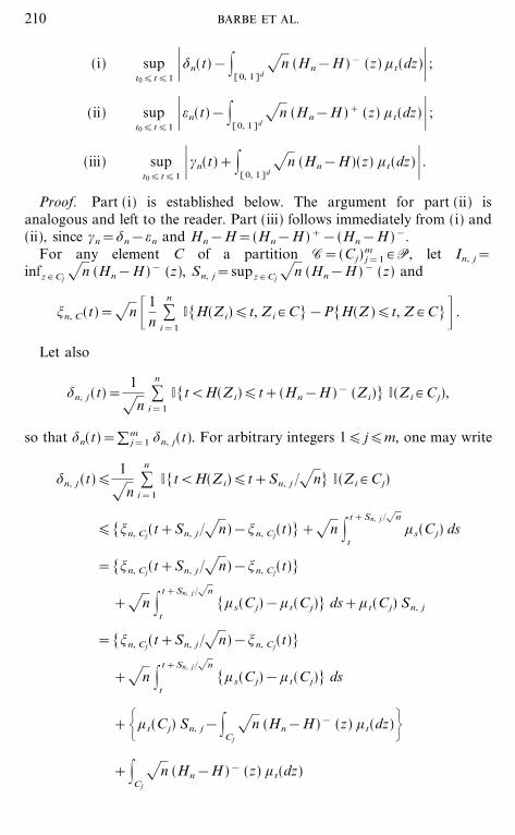
Proof. Part (i) is established below. The argument for part (ii) isanalogous and left to the reader. Part (iii) follows immediately from (i) and(ii), since #n=$n&=n and Hn&H=(Hn&H )+&(Hn&H )&.

For any element C of a partition C=(Cj)mj=1 # P, let In, j=

infz # Cj- n (Hn&H )& (z), Sn, j=supz # Cj

- n (Hn&H )& (z) and

!n, C(t)=- n _1n

:n

i=1

I[H(Zi)�t, Zi # C]&P[H(Z )�t, Z # C]& .

Let also

$n, j (t)=1

- n:n

i=1

I[t<H(Zi)�t+(Hn&H )& (Zi)] I(Zi # Cj),

so that $n(t)=�mj=1 $n, j(t). For arbitrary integers 1� j�m, one may write

$n, j (t)�1

- n:n

i=1

I[t<H(Zi)�t+Sn, j �- n] I(Zi # Cj)

�[!n, Cj(t+Sn, j �- n)&!n, Cj(t)]+- n |t+Sn, j �- n

t+s(Cj) ds

=[!n, Cj(t+Sn, j �- n)&!n, Cj(t)]

+- n |t+Sn, j �- n

t[+s(Cj)&+t(Cj)] ds++t(Cj) Sn, j

=[!n, Cj(t+Sn, j �- n)&!n, Cj(t)]

+- n |t+Sn, j �- n

t[+s(Cj)&+t(Cj)] ds

+{+t(Cj) Sn, j&|Cj

- n (Hn&H)& (z) +t(dz)=+|

Cj

- n (Hn&H )& (z) +t(dz)

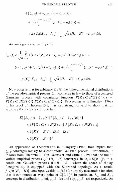
210 BARBE ET AL.


�[!n, Cj(t+Sn, j �- n)&!n, Cj(t)]

+- n |t+Sn, j �- n

t[+s(Cj)&+t(Cj)] ds

++t(Cj)(Sn, j&In, j)+|Cj

- n (Hn&H )& (z) +t(dz).

An analogous argument yields

$n, j(t)�1

- n:n

i=1

I[t<H(Zi)�t+In, j �- n] I(Zi # Cj)� } } }

�[!n, Cj(t+In, j �- n)&!n, Cj(t)]+- n |t+In, j �- n

t[+s(Cj)&+t(Cj)] ds

&+t(Cj)(Sn, j&In, j)+|Cj

- n (Hn&H )& (z) +t(dz).

Now observe that for arbitrary C # C, the finite-dimensional distributionsof the pseudo-empirical process !n, C converge in law to those of a centeredGaussian process with covariance function P[Z # C, H(Z )�t 7 s]&P[Z # C, H(Z )�t] P[Z # C, H(Z )�s]. Proceeding as Billingsley (1968)in his proof of Theorem 13.1, it is also straightforward to show that forarbitrary 0<u<s<t<1, one has

E[[!n, C(t)&!n, C(s)]2 [!n, C(s)&!n, C(u)]2]

�6P[Z # C, s<H(Z)�t] P[Z # C, u<H(Z )�s]

�6[K(t)&K(s)][K(s)&K(u)]

�6[K(t)&K(u)]2.

An application of Theorem 15.6 in Billingsley (1968) thus implies that!n, C converges weakly to a continuous Gaussian process. Furthermore, itfollows from Theorem 2.1.3 in Gaenssler and Stute (1979) that the multi-variate empirical process - n (Hn&H ) converges, in Dd=D[0, 1]d, to acontinuous Gaussian process B=B+&B&, where the space of ca� dla� gfunctions Dd is equipped with the Skorohod topology. As a result,f[- n (Hn&H )] converges weakly to f (B) for any Dd -measurable functionthat is continuous at every point of C[0, 1]d. In particular, In, j and Sn, j

converge in distribution to infz # Cj B&(z) and supz # Cj B&(z) respectively. As



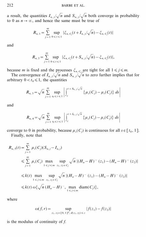
a result, the quantities In, j �- n and Sn, j �- n both converge in probabilityto 0 as n � �, and hence the same must be true of

Rn, 1= :m

j=1

sup0�t�1

|!n, Cj(t+In, j �- n)&!n, Cj(t)|

and

Rn, 2= :m

j=1

sup0�t�1

|!n, Cj(t+Sn, j �- n)&!n, Cj(t)|,

because m is fixed and the processes !n, Cj are tight for all 1� j�m.The convergence of In, j �- n and Sn, j �- n to zero further implies that for

arbitrary 0<t0�1, the quantities

Rn, 3=- n :m

j=1

supt0�t�1 } |

t+Sn, j �- n

t[+s(Cj)&+t(Cj)] ds }

and

Rn, 4=- n :m

j=1

supt0�t�1 } |

t+In, j �- n

t[+s(Cj)&+t(Cj)] ds }

converge to 0 in probability, because +s(Cj) is continuous for all s # [t0 , 1].Finally, note that

Rn, 5(t)= :m

j=1

+t(Cj)(Sn, j&In, j)

� :m

j=1

+t(Cj) max1� j�m

supz1 , z2 # Cj

- n |(Hn&H )& (z1)&(Hn&H )& (z2)|

�k(t) max1� j�m

supz1 , z2 # Cj

- n |(Hn&H )& (z1)&(Hn&H )& (z2)|

�k(t) |[- n (Hn&H )&, max1� j�m

diam(Cj)],

where

|( f, r)= supz1 , z2 # [0, 1]d, d(z1 , z2)�z

| f (z1)& f (z2)|

is the modulus of continuity of f.

212 BARBE ET AL.


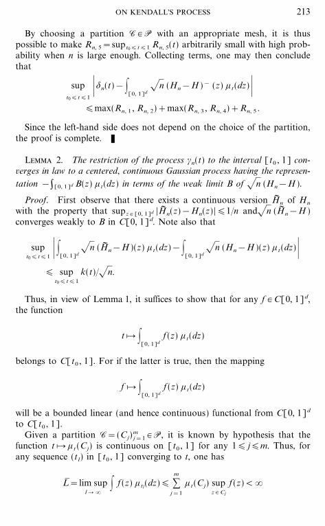
By choosing a partition C # P with an appropriate mesh, it is thuspossible to make Rn, 5=supt0�t�1 Rn, 5(t) arbitrarily small with high prob-ability when n is large enough. Collecting terms, one may then concludethat

supt0�t�1

} $n(t)&|[0, 1]d

- n (Hn&H )& (z) +t(dz) }�max(Rn, 1 , Rn, 2)+max(Rn, 3 , Rn, 4)+Rn, 5 .

Since the left-hand side does not depend on the choice of the partition,the proof is complete. K

Lemma 2. The restriction of the process #n(t) to the interval [t0 , 1] con-verges in law to a centered, continuous Gaussian process having the represen-tation &�[0, 1]d B(z) +t(dz) in terms of the weak limit B of - n (Hn&H ).

Proof. First observe that there exists a continuous version H� n of Hn

with the property that supz # [0, 1]d |H� n(z)&Hn(z)|�1�n and- n (H� n&H )converges weakly to B in C[0, 1]d. Note also that

supt0�t�1 } |[0, 1]d

- n (H� n&H )(z) +t(dz)&|[0, 1]d

- n (Hn&H )(z) +t(dz) }� sup

t0�t�1

k(t)�- n.

Thus, in view of Lemma 1, it suffices to show that for any f # C[0, 1]d,the function

t [ |[0, 1]d

f (z) +t(dz)

belongs to C[t0 , 1]. For if the latter is true, then the mapping

f [ |[0, 1]d

f (z) +t(dz)

will be a bounded linear (and hence continuous) functional from C[0, 1]d

to C[t0 , 1].Given a partition C=(Cj)

mj=1 # P, it is known by hypothesis that the

function t [ +t (Cj) is continuous on [t0 , 1] for any 1� j�m. Thus, forany sequence (tl) in [t0 , 1] converging to t, one has

L� =lim supl � �

| f (z) +tl(dz)� :m

j=1

+t(Cj) supz # Cj

f (z)<�



and

L�=lim inf

l � � | f (z) +tl(dz)� :m

j=1

+t(Cj) infz # Cj

f (z)>&�.

Consequently,

0�L� &L�� :

m

j=1

+t(Cj)[supz # Cj

f (z)& infz # Cj

f (z)]

� :m

j=1

+t(Cj) supz, w # Cj

| f (z)& f (w)|

�k(t) |[ f, max1� j�m

diam(Cj)].

Since this string of inequalities must hold whatever the choice of the parti-tion C, one may conclude that L� =L

�, whence the result. K

Lemma 3. For arbitrary *>0, one has

(i) limt0 � 0

lim supn � �

P( sup0�t�t0

$n(t)�*)=0;

(ii) limt0 � 0

lim supn � �

P( sup0�t�t0

=n(t)�*)=0;

(iii) limt0 � 0

lim supn � �

P( sup0�t�t0

|#n(t)|�*)=0.

Statement (iii) of this lemma is an immediate consequence of the firsttwo parts. To establish (i) and (ii), the following slight adaptation ofTheorem 2.4 of Alexander (1987) will be used.

Theorem 4. Let q be a nonnegative continuous function on [0, 1] suchthat q(t) is increasing and q(t)�t is decreasing in a positive neighborhood ofthe origin. Let also L(t)=max[1, log(t)] and for 0�t�1, define

�(t)=- 2t - L[ g(t)]+L[L(1�t)]

and

'(t)=q(t)

L[ g(t)]L _ q(t)

- tL[ g(t)]& ,

where g(t)=K(t)�t is bounded below by one for any copula H. Now supposethat q(t)��(t) � � when t � 0 and that (tn) is a sequence of nonnegative

214 BARBE ET AL.


numbers converging to zero such that n&1�2=o[inft�tn '(t)] as n � �. Thenas long as the copula H(z) is continuous, the process wn(z) defined for allz # [0, 1]d by

wn(z)=- nHn(z)&H(z)

q[H(z)]I[H(z)>tn]

converges weakly to a continuous Gaussian process having the representationB�q(H ).

Remark. In the statement of Theorem 4, K, Hn and B have the samemeaning as elsewhere in the paper. In particular, B is the weak limit of- n (Hn&H ) identified in the proof of Lemma 1. The inequality K(t)�tthat provides the lower bound on g is an immediate consequence of the factthat for arbitrary copula H, one has H(z(1), ..., z(d ))�z(i ) for all 1�i�d.

Corollary. Let q(t)=- t log p(1�t) and for arbitrary M>0, r>2p>1and integer n�1, let tn=logr(n)�n and denote by Fn, M the event

supz : H(z)>tn

- n|Hn(z)&H(z)|

q[H(z)]�M.

If k(t)=o[t&1�2 log&1�2&=(1�t)] as t � 0, then

limM � �

lim infn � �

P(Fn, M)=1

and

supz : H(z)>tn

|Hn(z)&H(z)|H(z)

�M log p&r�2(n) � 0

as n � � when Fn, M is realized.

Proof. In view of the fact that

1&P(Fn, M)�P( supz # [0, 1]d

|wn(z)|>M ),

the first conclusion of the corollary will be verified, provided that thesequence (supz |wn(z)| )n is tight. To see this, it suffices to verify the condi-tions of Theorem 4. It is easy to check that q(t) is nonnegative, continuousand increasing for 0<t<e&2p. It is also clear that q(t)�t is decreasing



on (0, 1]. Furthermore, the hypothesis on k(t) implies that K(t)=o[t1�2 log&1�2&=(1�t)] as t � 0. Consequently, K(t)�- t�log1�2+=(1�t) forall values of t in a positive neighborhood of the origin, and hence

q(t)

�(t)=

log p(1�t)

- n - log[ g(t)]+log[log(1�t)]

�log p&1�2(1�t)

- 1+(1&2=) log[log(1�t)]�log(1�t),

which tends to infinity as t � 0, because p>1�2.Next, observe that for t>0 small enough, one has

q(t)�- n �(t)�2 - t log[ g(t)] .

Since '(t) is a monotone function of q(t) and g(t)=K(t)�t�1�t, it followsthat

'(t)�2 - t log[ g(t)]

log[ g(t)]log _2 - t log[ g(t)]

- t log[ g(t)] &�� t

log(1�t)

in a positive neighborhood of the origin. As a result,

n inft�tn

['2(t)]�n inft�tn {

tlog(1�t)==

ntn

log(1�tn)

=logr&1(n)

1&r log[log(n)]�log(n)� �

when n � �, which completes the verification of Alexander's conditions.Finally, assume that Fn, M is realized. It then follows from the decreasing-

ness of q(t)�t that

supz : H(z)�tn

|Hn(z)&H(z)|H(z)

= supz : H(z)�tn

|Hn(z)&H(z)|q[H(z)]

q[H(z)]H(z)

�M

- nsup

tn�t�1

q(t)

t

=Mq(tn)

- n tn

�M log p&r�2(n),

which goes to 0 as n � � because r>2p by hypothesis. K

216 BARBE ET AL.


Proof of Lemma 3. (i). Choose p and r such that 1<2p<r�1+2=,and for given *>0, write

P[ sup0�t�t0

$n(t)�*]�P[ sup0�t�t0

$n(t)�*, Fn, M]+[1&P(Fn, M)].

In view of the above corollary, the right-most term can be made arbitrarilysmall by choosing M large enough. The proof will thus be complete if onecan show that for any fixed M, one has

lim supt0 � 0

lim supn � �

P[ sup0�t�t0

$n(t)�*, Fn, M]=0.

To this end, observe that

[t<H(Zi)�t+(Hn&H )& (Zi)]=[Hn(Zi)�t<H(Zi)]

so that when n is sufficiently large that M log p&r�2(n)�1�2, one finds

Fn, M & [t<H(Zi)�t+(Hn&H )& (Zi)] & [H(Zi)�tn]

=Fn, M & {t<H(Zi)�t+M

- nq[H(Zi)]=& [Hn(Zi)�t<H(Zi)]

& [H(Zi)�tn].

But it follows from the corollary that for such n,

Fn, M & [H(Zi)�tn]/{Hn(Zi)H(Zi)

�12= ,

and hence

Fn, M & [Hn(Zi)�t<H(Zi)] & [H(Zi)�tn]/[H(Zi)�2t].

Consequently,

Fn, M & [t<H(Zi)�t+(Hn&H )& (Zi)] & [H(Zi)�tn]

/{t<H(Zi)�t+M

- nq(2t)= .



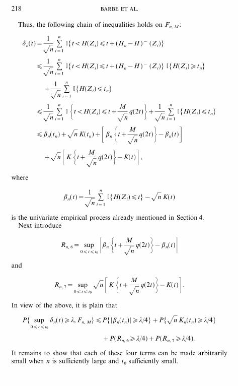
Thus, the following chain of inequalities holds on Fn, M :

$n(t)=1

- n:n

i=1

I[t<H(Zi)�t+(Hn&H )& (Zi)]

�1

- n:n

i=1

I[t<H(Zi)�t+(Hn&H )& (Zi)] I[H(Zi)�tn]

+1

- n:n

i=1

I[H(Zi)�tn]

�1

- n:n

i=1

I {t<H(Zi)�t+M

- nq(2t)=+

1

- n:n

i=1

I[H(Zi)�tn]

�;n(tn)+- n K(tn)+_;n {t+M

- nq(2t)=&;n(t)&

+- n _K {t+M

- nq(2t)=&K(t)& ,

where

;n(t)=1

- n:n

i=1

I[H(Zi)�t]&- n K(t)

is the univariate empirical process already mentioned in Section 4.Next introduce

Rn, 6= sup0�t�t0

};n {t+M

- nq(2t)=&;n(t) }

and


- n _K {t+M

- nq(2t)=&K(t)& .

In view of the above, it is plain that

P[ sup0�t�t0

$n(t)�*, Fn, M]�P[ |;n(tn)|�*�4]+P[- n Kn(tn)�*�4]

+P(Rn, 6�*�4)+P(Rn, 7�*�4).

It remains to show that each of these four terms can be made arbitrarilysmall when n is sufficiently large and t0 sufficiently small.

218 BARBE ET AL.


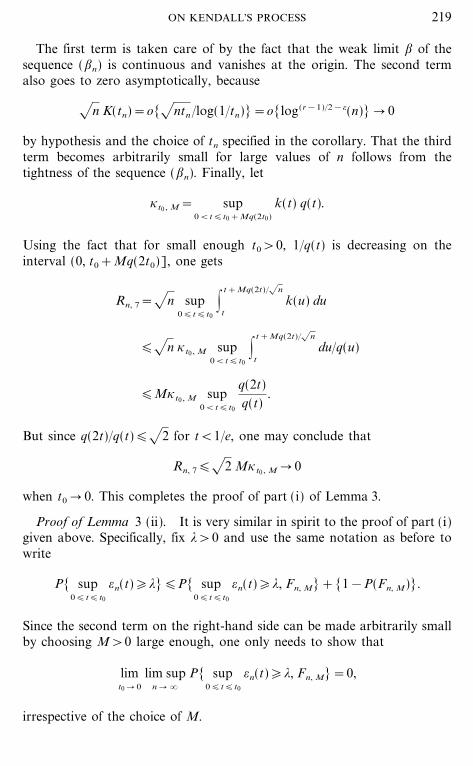
The first term is taken care of by the fact that the weak limit ; of thesequence (;n) is continuous and vanishes at the origin. The second termalso goes to zero asymptotically, because

- n K(tn)=o[- ntn�log(1�tn)]=o[log(r&1)�2&=(n)] � 0

by hypothesis and the choice of tn specified in the corollary. That the thirdterm becomes arbitrarily small for large values of n follows from thetightness of the sequence (;n). Finally, let

}t0 , M= sup0<t�t0+Mq(2t0)

k(t) q(t).

Using the fact that for small enough t0>0, 1�q(t) is decreasing on theinterval (0, t0+Mq(2t0)], one gets

Rn, 7=- n sup0�t�t0

|t+Mq(2t)�- n

tk(u) du

�- n }t0 , M sup0<t�t0

|t+Mq(2t)�- n

tdu�q(u)

�M}t0 , M sup0<t�t0

q(2t)q(t)

.

But since q(2t)�q(t)�- 2 for t<1�e, one may conclude that

Rn, 7�- 2 M}t0 , M � 0

when t0 � 0. This completes the proof of part (i) of Lemma 3.

Proof of Lemma 3 (ii). It is very similar in spirit to the proof of part (i)given above. Specifically, fix *>0 and use the same notation as before towrite

P[ sup0�t�t0

=n(t)�*]�P[ sup0�t�t0

=n(t)�*, Fn, M]+[1&P(Fn, M)].

Since the second term on the right-hand side can be made arbitrarily smallby choosing M>0 large enough, one only needs to show that

limt0 � 0

lim supn � �

P[ sup0�t�t0

=n(t)�*, Fn, M]=0,

irrespective of the choice of M.



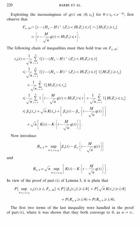
Exploiting the increasingness of q(t) on (0, t0] for 0<t0<e&2p, firstobserve that

Fn, M & [t&(Hn&H )+ (Zi)<H(Zi)�t] & [H(Zi)�tn]

/{t&M

- nq(t)<H(Zi)�t= .

The following chain of inequalities must then hold true on Fn, M :

=n(t)=1

- n:n

i=1

I[t&(Hn&H )+ (Zi)<H(Zi)�t]

�1

- n:n

i=1

I[t&(Hn&H )+ (Zi)<H(Zi)�t] I[H(Zi)�tn]

+1

- n:n

i=1

I[H(Zi)�tn]

�1

- n:n

i=1

I {t&M

- nq(t)<H(Zi)�t=+

1

- n:n

i=1

I[H(Zi)�tn]

�;n(tn)+- n K(tn)+_;n(t)&;n {t&M

- nq(t)=&

+- n _K(t)&K {t&M

- nq(t)=& .

Now introduce


};n(t)&;n {t&M

- nq(t)=}

and

Rn, 9=- n sup0�t�t0

_K(t)&K {t&M

- nq(t)=& .

In view of the proof of part (i) of Lemma 3, it is plain that

P[ sup0�t�t0

=n(t)�*, Fn, M]�P[ |;n(tn)|�*�4]+P[- n K(tn)�*�4]

+P(Rn, 8�*�4)+P(Rn, 9�*�4).

The first two terms of the last inequality were handled in the proofof part (i), where it was shown that they both converge to 0, as n � �.

220 BARBE ET AL.


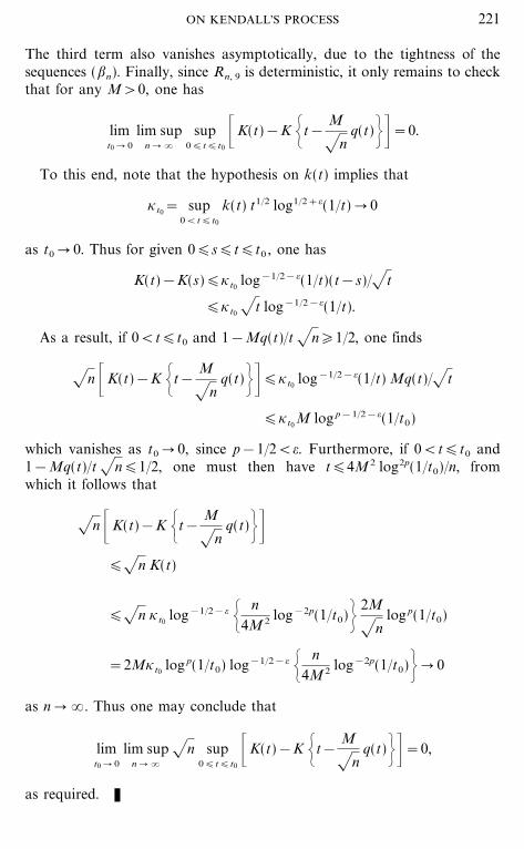
The third term also vanishes asymptotically, due to the tightness of thesequences (;n). Finally, since Rn, 9 is deterministic, it only remains to checkthat for any M>0, one has

limt0 � 0

lim supn � �

sup0�t�t0

_K(t)&K {t&M

- nq(t)=&=0.

To this end, note that the hypothesis on k(t) implies that

}t0= sup

0<t�t0

k(t) t1�2 log1�2+=(1�t) � 0

as t0 � 0. Thus for given 0�s�t�t0 , one has

K(t)&K(s)�}t0log&1�2&=(1�t)(t&s)�- t

�}t0- t log&1�2&=(1�t).

As a result, if 0<t�t0 and 1&Mq(t)�t - n�1�2, one finds

- n _K(t)&K {t&M

- nq(t)=&�}t0

log&1�2&=(1�t) Mq(t)�- t

�}t0M log p&1�2&=(1�t0)

which vanishes as t0 � 0, since p&1�2<=. Furthermore, if 0<t�t0 and1&Mq(t)�t - n�1�2, one must then have t�4M2 log2p(1�t0)�n, fromwhich it follows that

- n _K(t)&K {t&M

- nq(t)=&

�- n K(t)

�- n }t0log&1�2&= { n

4M 2 log&2p(1�t0)= 2M

- nlog p(1�t0)

=2M}t0log p(1�t0) log&1�2&= { n

4M2 log&2p(1�t0)=� 0

as n � �. Thus one may conclude that

limt0 � 0

lim supn � �

- n sup0�t�t0

_K(t)&K {t&M

- nq(t)=&=0,

as required. K



6. WEAK CONVERGENCE OF :n AND :n*

In order to identify the weak limit of the sequence (:n*), it will be con-venient to introduce an empirical process indexed by a class of measurablesubsets of [0, 1]d. The following definitions and notations are taken fromPollard (1984). Alternative references on this topic include Dudley (1984),and Ledoux and Talagrand (1991).

Let A1 be the collection of sets of the form A1, z=[z$ # [0, 1]d : z$�z].Let also A2 represent the family of sets of the form A2, t=[z # [0, 1]d : H(z)�t] with 0�t�1. The union A of these two classes willbe used as the index set for the empirical process &n defined by

&n(A)=- n {1n

:n

i=1

I(Zi # A)&P(Z # A)= , A # A.

Observe that &n(A1, z)=- n (Hn&H )(z) for all z # [0, 1]d and that&n(A2, t)=;n(t) for all t # [0, 1]. Note also that the representation

|[0, 1]d

- n (Hn&H )(z) +t(dz)=|[0, 1]d

&n(A1, z) +t(dz)

is valid for all 0�t�1.It is easy to see that A is a Vapnik�C2 ervonenkis class. This implies that

&n converges weakly to a centered Gaussian process & over A that is con-tinuous with respect to the pseudo-metric \ defined for arbitrary A, A$ # Aby

\(A, A$)=P(Z # A"A$)+P(Z # A$"A).

It also implies that the covariance structure of the limiting process & isgiven by

E[&(A) &(A$)]=P(Z # A & A$)&P(Z # A) P(Z # A$),

for all A, A$ # A.With these notations, it is now possible to give a representation of the

process : that constitutes the limit of the sequence (:n).

Theorem 5. The sequence (:n*) converges weakly to a continuous cen-tered Gaussian process : with covariance function

1(s, t)=K(s 7 t)&K(s) K(t)+k(s) k(t) R(s, t)&k(t) Q(s, t)&k(s) Q(t, s)

222 BARBE ET AL.


expressed for all 0�s, t�1 in terms of functions Q and R defined inSection 2. Moreover, the limiting process has the following representation interms of &:

:(t)=&(A2, t)&|[0, 1]d

&(A1, z) +t(dz), t # [0, 1].

Proof. Recall that :n*(t) may be written as ;n(t)+#n(t). Given0<t0�1, it follows from Lemmas 1 and 2 that :n*(t) converges weakly toa continuous process :(t) that may be represented as above for t0�t�1.From Lemma 3 and the fact that the limit ; of the sequence (;n) is con-tinuous and vanishes at the origin, one may also assert that

limt0 � 0

lim supn � �

P[ sup0�t�t0

|:n*(t)|�*]=0

whatever the value of *>0. Consequently, :n*(t) converges weakly to :(t)as defined above. Note that this process actually vanishes at the origin.

It remains to check that E[:(s) :(t)]=1(s, t) for all 0�s, t�1. To thisend, first note that

E[&(A2, s) &(A2, t)]=P[H(Z )�s 7 t]&P[H(Z )�s] P[H(Z )�t]

=K(s 7 t)&K(s) K(t).

Next, observe that

E {&(A2, s) |[0, 1]d

&(A1, z) +t(dz)==|[0, 1]d

P[H(Z )�s, Z�z1] +t(dz1)

&|[0, 1]d

P[H(Z )�s] P(Z�z1) +t(dz1)

=k(t) Q(s, t).

Interchanging the roles of s and t, one also gets

E {&(A2, t) |[0, 1]d

&(A1, z) +s(dz)==k(s) Q(t, s).

Finally, a similar calculation yields

E {|[0, 1]d&(A1, z) +s(dz) |

[0, 1]d&(A1, z) +t(dz)=

=|[0, 1]d |[0, 1]d

P(Z�z1 7 z2) +s(dz1) +t(dz2)

&|[0, 1]d |[0, 1]d

P(Z�z1) P(Z�z2) +s(dz1) +t(dz2)

=k(s) k(t) R(s, t).



Combining these four terms yields the appropriate expression for 1. K

Proof of Theorem 1. In view of the above result, it only remains toshow that sup0�t�1 |:n(t)&:n*(t)| converges to 0 in probability. The argu-ment is based on the following identity, which holds true for all n�1 and0�t�1:

:n(t)=:n*[t+(1&t)�n]+- n [K[t+(1&t)�n]&K(t)].

An application of the triangle inequality yields

sup0�t�1

|:n(t)&:n*(t)|� sup0�t�1

|:n*[t+(1&t)�n]&:n*(t)|

+- n sup0�t�1

[K(t+1�n)&K(t)].

But the first term on the right-hand side converges to zero in probabilitybecause the sequence (:n*) is tight. To handle the second term, first observethat for 0<t�1�n, one has

- n sup0<t�1�n

[K(t+1�n)&K(t)]�- n K(2�n)=o[log&1�2&=(n)] � 0

as n � �. Next, since the function q(t)=- t log p(1�t) is increasing on theinterval [1�n, e&2p], one has

- n sup1�n�t�e&2p

[K(t+1�n)&K(t)]�- n

q(1�n)sup

1�n�t�e&2p |t+1�n

tk(u) q(u) du

�[ sup0<t�1

k(t) q(t)]1

nq(1�n)� 0

as n � �. Finally, if e&2p�t�1, k(t) is bounded on that interval. There-fore,

- n supe&2p�t�1

[K(t+1�n)&K(t)]�1

- nsup

e&2p�t�1

k(t) � 0

as n � �. Combining these three estimates, one gets

limn � �

sup0�t�1

- n [K(t+1�n)&K(t)]=0.

This completes the proof. K

224 BARBE ET AL.


7. PROOF OF THEOREM 2

The proof is given in two steps. The first consists in showing that aversion of the conditional distribution of Z given H(Z )=t can be foundsuch that for any continuous f on [0, 1]d, the mapping t [ gt( f )=�(0, 1)d f (z) +t(dz) is continuous on (0, 1]. The second step will then consistof showing that the function t [ +t(C ) is continuous on (0, 1] for any non-empty rectangle C=[z # [0, 1]d : z1<z�z2].

Step 1. Let f be a continuous function on [0, 1]d, and define

Gt ( f )=E[ f (Z) I[H(Z )�t]], t # [0, 1].

It follows that

Gt( f )=|(0, 1)d&1 |

1

0f (x, y) h(x, y) I[H(x, y)�t] dy dx.

Upon letting s=H(x, y) for fixed x verifying H(x, 1)>s, one obtainsy=Qx[s�H(x, 1)] and dy�ds=dQx[s�H(s, 1)]�ds. Hence

Gt( f )=|(0, 1)d&1 |

t

0f[x, Qx[s�H(x, 1)]] hs(x) ds dx

=|t

0 \|(0, 1)d&1f[x, Qx[s�H(x, 1)]] hs(x) dx+ ds.

From the very definition of +t , it follows that

Gt( f )=|t

0|

(0, 1)df (z) +s(dz) ds.

Consequently +t is a version of k(t) times the conditional distribution ofZ given H(Z )=t for which the mapping

t [ gt( f )=|(0, 1)d

f (z) +t(dz)=|(0, 1)d

f[x, Qx[t�H(x, 1)]] ht(x) dx

is continuous on (0, 1) for all continuous function f on [0, 1]d, because thelatter and h are themselves continuous and because the derivative of Qx(t)is continuous on (0, 1). As a special case, taking f identically equal to one,one obtains

k(t)=|(0, 1)d&1

ht(x) dx, t # (0, 1).



Next, recall that H(z)�min1�i�d z(i ), so that H(z)=1 if and onlyif z=(1, ..., 1). Hence E[ f (Z ) | H(Z)=1]= f (1, ..., 1) and g1( f )=�(0, 1)d f (z) +1(dz)=k(1) f (1, ..., 1). It remains to show that gt( f ) convergesto g1( f ) as t tends to 1.

At this point, note that if s<t, then H(x, s)�s<t. Thus if H(x, 1)>t,one gets Hd(s | x)<t�H(x, 1), yielding Qx[t�H(x, 1)]>s. As the lastinequality holds true for all s<t, it follows that Qx[t�H(x, 1)]�t.Moreover, H(x, 1)>t implies that x(i )>t for all 1�i�d&1. Conse-quently, one finds

| g1( f )& gt( f )|�| f (1, ..., 1)| |k(1)&k(t)|

+|(0, 1)d&1 } f _x, Qx { t

H(x, 1)=&& f (1, ..., 1) } ht(x) dx

�| f (1, ..., 1)| |k(1)&k(t)|

+k(t) supx : H(x, 1)>t } f _x, Qx { t

H(x, 1)=&& f (1, ..., 1) }�| f (1, ..., 1)| |k(1)&k(t)|

+k(t) supz # [t, 1]d

| f (z)& f (1, ..., 1)| � 0

as t � 1, because k is continuous on (0, 1] and f is continuous on [0, 1]d.

Step 2. What needs to be shown is that for fixed t # (0, 1], the map-ping s [ +s(C ) is continuous at t for any non-empty rectangle C of theform [z # [0, 1]d : z1<z�z2].

First consider the case where t<1. Given a rectangle C of the aboveform, it will be sufficient to show that +t[z : z(i )=c]=0 for arbitraryc # [0, 1] and 1�i�d. For, since the boundary of C is included in a finiteunion of sets of the form [z : z(i )=c], it will then follow that +t(�C)=0.As a result, one will conclude that lims � t +s(C )=+t(C ) from the con-tinuity of +s .

It is sufficient to consider c # (0, 1) since +t[[t, 1)d]=1. In view of therepresentation

|(0, 1)d

f (x) +t(dx_dy)=|(0, 1)d&1

f (x) ht(x) dx,

valid for any continuous function f on [0, 1]d&1, the measure +t b ?&1d has

density ht(x) with respect to Lebesgue measure. Hence +t[z : z(i )=c]=0for arbitrary c # (0, 1) and 1�i�d&1. To handle the case i=d, let�d H(x, c) denote the partial derivative of H(z) with respect to z(d ) at point

226 BARBE ET AL.


z=(x, c). In view of the representation of +t in terms of ht(x) andQx[t�H(x, 1)], one has

+t[z # [0, 1]d : z(d )=c]=|(0, 1)d&1

h(x, c)�d H(x, c)

I[x # (0, 1)d&1: H(x, c)=t] dx.

First suppose that d=2. In that case, the Lebesgue measure of the set[x # [0, 1] : H(x, c)=t] is greater than 0 if and only if there exist0<a<b�1 such that [a, b]=[x # [0, 1] : H(x, c)=t]. As a result, onefinds

0=H(b, c)&H(a, c)=|b

a|

c

0h(x, y) dy dx.

Since h is continuous, it follows that h(x, c)=0 for all x # [a, b], whence+t[z # [0, 1]2 : z(2)=c]=0, completing the proof.

Next, suppose that d>2 and introduce the open set O=[x # (0, 1)d&1:h(x, c)>0]. Then

+t[z # [0, 1]d : z(d )=c]=|O

h(x, c)�d H(x, c)

I[x # (0, 1)d&1 : H(x, c)=t] dx.

Thus, the argument will be complete if one can show that the Lebesguemeasure of the set [x # (0, 1)d&1: H(x, c)=t] & O is zero. To this end, theImplicit Function Theorem (Theorem 9.28 in Rudin, 1976) can be appliedto the function f (x)=H(x, c)&t for x # O. Note that this mapping of Ointo R is continuously differentiable and that its derivative with respectto x(1) is greater than zero for any x # O. Therefore, for any x # O suchthat f (x)=0, that is H(x, c)=t, there exist open sets Wx/(0, 1)d&2,and a continuously differentiable mapping gx of Wx into (0, 1) so thatx(1)= gx[x(2), ..., x(d&1)] and H[ gx(w), w, c]=t for all w # Wx .

It is remarkable that if w # Wx1& Wx2

for some x1{x2 both belonging toO, then gx1

(w)= gx2(w). For, if this were false, then one would get

H(b, w, c)&H(a, w, c)=0 for b=max[ gx1(w), gx2

(w)] and a=min[ gx1(w),

gx2(w)], yielding h(s, w, c)=0 for all s # [a, b]; but this would contradict

the fact that ( gx1(w), w) and ( gx2

(w), w) both belong to O. As a result,there exists a continuously differentiable mapping g of the open setW=�x # O Wx into (0, 1), defined by g(w)= gx(w) if w # Wx , so that

[x # (0, 1)d&1: H(x, c)=t] & O=[( g(w), w) : w # W]

has Hausdorff dimension d&2, proving that the set [x # (0, 1)d&1:H(x, c)=t] & O is negligible with respect to Lebesgue measure on(0, 1)d&1.



It remains to look at the case t=1. If C=[z # [0, 1]d : z1<z�z2] andz2{(1, ..., 1), then (1, ..., 1) � �C, and hence it follows from the continuityof + that +1(�C )=0 and +s(C ) � +1(C ), as s � 1. If z2=(1, ..., 1), then+1(C )=k(1) and +s(C )=k(s) whenever s>max1�i�d z (i )

1 , becausefor such s, H(x, 1)>s yields (x, Qx[s�H(x, 1)])/[s, 1]d/C. Sincek(s) � k(1) as s � 1, the proof is complete. K

ACKNOWLEDGMENTS

Research funds in partial support of this work were granted by the Natural Sciences andEngineering Research Council of Canada, the Fonds pour la formation de chercheurs et l'aidea� la recherche du Gouvernement du Que� bec, and the Fonds institutionnel de la recherche del'Universite� du Que� bec a� Trois-Rivie� res.

REFERENCES

Alexander, K. S. (1987). The central limit theorem for weighted empirical processes indexedby sets. J. Multivariate Anal. 22 313�339.

Ali, M. M., Mikhail, N. N., and Haq, M. S. (1978). A class of bivariate distributions includingthe bivariate logistic. J. Multivariate Anal. 8 405�412.

Billingsley, P. (1968). Convergence of Probability Measures. Wiley, New York.Clayton, D. G. (1978). A model for association in bivariate life tables and its applications in

epidemiological studies of familial tendency in chronic disease incidence. Biometrika 65141�151.

de la Horra, J., and Fernandez, C. (1995). Sensitivity to prior independence via Farlie�Gumbel�Morgenstern model. Comm. Statist. Theory Methods 24 987�996.

Dudley, R. M. (1984). A course on empirical processes. In E� cole d 'e� te� de probabilite� s de Saint-Flour, XII-1982. Lecture Notes in Mathematics, Vol. 1097, pp. 1�142. Springer, New York.

Frank, M. J. (1979). On the simultaneous associativity of F(x, y) and x+ y&F(x, y). Squa-tiones Math. 19 194�226.

Gaenssler, P., and Stute, W. (1979). Empirical processes: A survey of results for independentand identically distributed random variables. Ann. Probab. 7 193�243.

Genest, C. (1987). Frank's family of bivariate distributions. Biometrika 74 549�555.Genest, C., and MacKay, R. J. (1986a). Copules archime� diennes et familles de lois bidimen-

sionnelles dont les marges sont donne� es. Canad. J. Statist. 14 145�159.Genest, C., and MacKay, R. J. (1986b). The joy of copulas: Bivariate distributions with

uniform marginals. Amer. Statist. 40 280�283.Genest, C., and Rivest, L.-P. (1993). Statistical inference procedures for bivariate

Archimedean copulas. J. Amer. Statist. Assoc. 88 1034�1043.Gumbel, E. J. (1960). Distribution des valeurs extremes en plusieurs dimensions. Publ. Inst.

Statist. Univ. Paris 9 171�173.Joe, H. (1990). Multivariate concordance. J. Multivariate Anal. 35 12�30.Ledoux, M., and Talagrand, M. (1991). Probability in Banach Spaces. Springer, Berlin.Lee, A. J. (1985). U-Statistics: Theory and Practice. Dekker, New York.

228 BARBE ET AL.


Nelsen, R. B. (1986). Properties of a one-parameter family of bivariate distributions withspecified marginals. Comm. Statist. Theory Methods 15 3277�3285.

Pollard, D. (1984). Convergence of Stochastic Processes. Springer, Berlin.Rudin, W. (1976). Principles of Mathematical Analysis, 3rd ed. McGraw�Hill, New York.Sklar, A. (1959). Fonctions de re� partition a� n dimensions et leurs marges. Publ. Inst. Statist.

Univ. Paris 8 229�231.


On Kendall's Process

Documents

Transcript of On Kendall's Process