On Bridging the Gap between Tree-Level and Stand-Level Models
12
On Bridging the Gap between Tree-Level and Stand-Level Models Oscar García University of Northern British Columbia 3333 University Way, Prince George, B.C., Canada V2N 4Z9 [email protected] http://web.unbc.ca/~garcia Abstract. Individual-based and aggregated models for forest stands are compared. This is followed by a brief review of research on mathematical analysis of complex simulation models, and the derivation of simpler analytical approximations. Finally, a statistical top-down approach is demonstrated, with a three-dimensional state space model that approximates stand development predicted by the TASS tree-level simulator. 1 Introduction Forest growth models have been developed with various levels of detail, and with an emphasis on either mechanistic process representation or on accurate long-term forecasting. The most appropriate model types depend on intended use, stand characteristics, and other circumstances. Although communication and collaboration between proponents of different approaches has generally been poor, there is scope for establishing links between model types to make better use of their specific strengths. I will discuss two possible approaches to developing these links to bridge the gap between the modelling paradigms. In the first, a constructive, deductive, or “bottom- up” approach, one seeks to mathematically derive an aggregated model from a detailed individual-based model through a process of aggregation and simplification. The second, a predictive or “top-down” approach, is less mathematical and more statistical in nature: an independent aggregated model is built, attempting to approximate the global behaviour of the more detailed one. Some concepts and terminology are presented first, followed by the implications of dimensionality for different applications. After a brief review of bottom-up approaches, the top-down route is illustrated with a stand-level approximation to a complex tree-level growth model. 2 Dynamic Models, Resolution Level The classical yield tables were a remarkable achievement of early mathematical modelling. By the 18th Century foresters had discovered that it was not necessary to
-
Upload
independent -
Category
Documents
-
view
0 -
download
0
Transcript of On Bridging the Gap between Tree-Level and Stand-Level Models
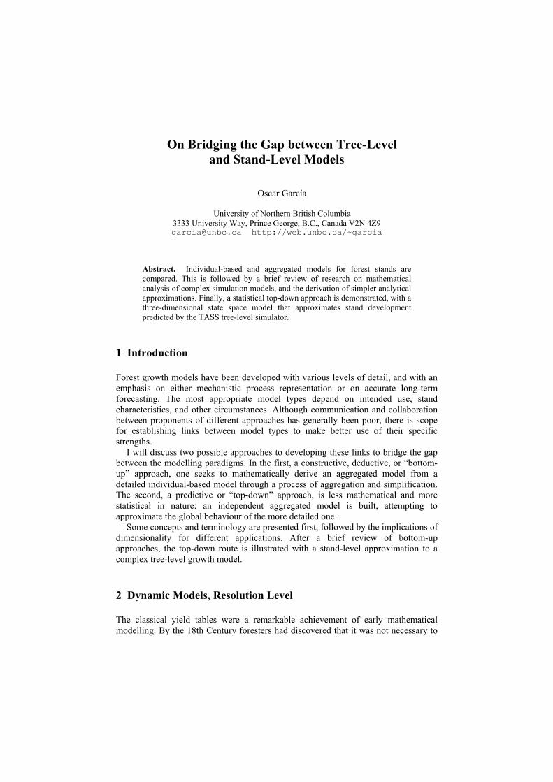
On Bridging the Gap between Tree-Level and Stand-Level Models
Oscar García
University of Northern British Columbia 3333 University Way, Prince George, B.C., Canada V2N 4Z9 [email protected] http://web.unbc.ca/~garcia
Abstract. Individual-based and aggregated models for forest stands are compared. This is followed by a brief review of research on mathematical analysis of complex simulation models, and the derivation of simpler analytical approximations. Finally, a statistical top-down approach is demonstrated, with a three-dimensional state space model that approximates stand development predicted by the TASS tree-level simulator.
1 Introduction
Forest growth models have been developed with various levels of detail, and with an emphasis on either mechanistic process representation or on accurate long-term forecasting. The most appropriate model types depend on intended use, stand characteristics, and other circumstances. Although communication and collaboration between proponents of different approaches has generally been poor, there is scope for establishing links between model types to make better use of their specific strengths.
I will discuss two possible approaches to developing these links to bridge the gap between the modelling paradigms. In the first, a constructive, deductive, or “bottom-up” approach, one seeks to mathematically derive an aggregated model from a detailed individual-based model through a process of aggregation and simplification. The second, a predictive or “top-down” approach, is less mathematical and more statistical in nature: an independent aggregated model is built, attempting to approximate the global behaviour of the more detailed one.
Some concepts and terminology are presented first, followed by the implications of dimensionality for different applications. After a brief review of bottom-up approaches, the top-down route is illustrated with a stand-level approximation to a complex tree-level growth model.
2 Dynamic Models, Resolution Level
The classical yield tables were a remarkable achievement of early mathematical modelling. By the 18th Century foresters had discovered that it was not necessary to

wait a full rotation to estimate growth trajectories; observations over shorter intervals in stands of various ages (cross-sectional or panel data) could instead be pieced together. For many purposes, this type of “static” model is still adequate. In other circumstances, however, more flexibility is needed. Yield tables (or functions) cannot deal cleanly with arbitrary deviations from a trend caused by thinnings of varied timing and intensity. Even without thinning, projections for existing stands that have deviated from the average curve can be cumbersome. A truly dynamic model is then desirable.
Although long established in other disciplines, the general principles of dynamic modelling have only recently begun to be generally understood and accepted in forestry. The basic idea is not attempting to develop directly the trend of variables over time, as in yield tables. Instead, the state of a stand at a point in time is described by a certain number of variables, and equations are obtained to predict the rate of change over time of this state (e.g., Zadeh 1969; Kalman et al. 1969; García 1994). Given the initial state, these rates can be summed or integrated to compute the future state trajectory. A thinning produces an instantaneous change of state, and the projection can then be resumed from the new state.
Different growth model types differ in the level of detail represented in the state description. Tree-level models specify the diameter, and possibly height and/or other variables, for each tree in a stand or sample plot. Stand-level models describe the stand by a small number of aggregate “macro” variables, such as mean diameter, top height, trees per hectare.
Tree-level models can be spatial (or distance-dependent, spatially explicit, spatially extended), if the position of each tree on the ground is part of the state description, or aspatial, (distance-independent, etc.), if it is not. Alternatively, aspatial tree-level models are sometimes classified as distribution-based models; a set of tree sizes (a “tree list”) being equivalent to an empirical distribution. The distribution-based category may include models where the state is a continuous size distribution specified by a few parameters or moments, which could also be considered as stand-level.
3 High-Dimensional vs. Low-Dimensional States
In most instances, the benefits of modelling are multiple. It is useful, however, to distinguish between situations where the primary purpose of the model is decision-making (prediction), and those where it is used mainly as a research tool (understanding).
3.1 Prediction
For planning and forest management purposes, one is often more interested in accurate and precise growth projections than in attempting to mimic the underlying processes. Even so, the conceptual simplicity and well-defined mechanisms of tree-level models can make them more appropriate when there is limited data. It is generally easier to build from first principles a tree-level model that produces

plausible (not necessarily correct!) results. Relationships can be fitted to tree-level data which, although more detailed, do not need to proceed from stands covering a wide range of growing conditions (ages and stand densities), as is necessary for properly estimating stand-level models.
In addition, tree-level models may be the best or only option for complex stands, those that are uneven-aged and/or contain a multitude of species. Where there are alternatives, there seems to be general agreement that, in principle, stand-level models should be more accurate and precise. Problems of over-parameterization and accumulation of errors tend to be more serious in tree-level models. To realize this potential, however, adequate model structure, data, and estimation techniques are needed.
Much analysis of the reliability of predictions has focused on the effect of estimation errors and uncertainty in the model parameters (e.g., Gertner 1987; Green 1999). Less attention has been given to uncertainty in the initial state. Rarely, if ever, do we have precise knowledge of the size (and location for spatial models) of every tree in a stand. More often, forest inventories only provide acceptable estimates of a few aggregates, such as basal area and number of trees per hectare, top height, etc. In order to use a tree-level model for prediction, therefore, it is necessary to artificially generate a detailed initial state given our limited knowledge of stand-level variables. Numerous procedures involving random numbers have been used or proposed for both aspatial “tree list generation” (www.ubc.ca/forestry/treelist/), and for simulating spatial patterns. Usually, the projected tree-level attributes are summarized into stand-level variables for their use in decision-making.
It is clear that if the detailed tree-level information is really necessary to predict behaviour, as might be the case in complex stands, no amount of numeric manipulation will be able to substitute for the missing component. One must accept the fact that uncertainty about the future will be at best similar to that about the present. If, on the contrary, the tree-level description can be reliably estimated from stand-level variables, then that information is redundant for prediction purposes. At least in principle, the data could be projected directly by a stand-level model (Fig. 1).

Fig. 1. Projection of stand attributes with tree-level and stand-level models
It may be worth mentioning that the often-heard argument in favour of tree-level models, that unlike stand-level models they produce useful information in the form of size distributions and such, does not hold. If the initial distribution can be satisfactorily estimated from stand-level variables, the same should be true at the end of the projection interval (upward pointing arrow to the right of Fig. 1). It must also be kept in mind that because of spatial structure, distributions for a whole stand, what one usually wants, can be quite different from distributions within sample plots, what one usually gets (García 1992).
3.2 Understanding
Where modelling is mainly a research tool, used to investigate processes of stand development, tree-level models can be very useful. Here, qualitative agreement with hypothesized mechanisms is paramount, while questions of quantitative accuracy and precision are largely irrelevant. Often the benefits arise mainly from building the model, through synthesis of previously isolated facts and identification of gaps in knowledge. Highly detailed spatial models are likely to be the most useful, at least in the early stages of understanding.
Foresters were pioneers in individual-based spatial modelling. Following early work by Staebler in 1951, the idea really took off with the availability of digital computers in the mid-60's, notably in the dissertations of Newnham and others at the University of British Columbia under J. H. G. Smith. The peak of activity was reached in the 1970's. See Dudek and Ek (1980) for an annotated bibliography. Many

(most?) of these models were ultimately intended to be used for forest management, not only as research tools.
Incidentally, the great majority of spatial forest growth models, and perhaps all aspatial ones, use the tree diameters as the main or only driving state variables. From a biological point of view this may be seen as a limitation: tree growth rates are not driven by the amount of wood that has accumulated on the stem, rather this is a consequence of growing-space-dependent growth rates. There is often a good correlation between diameter, growing space and other variables, especially in unmanaged natural stands where most of the work has been done. This correlation, however, breaks down whith stand intervention.
Two decades later, individual-based or multiagent-based simulation was “discovered” in population ecology, physics, economics, sociology, and geography. There was an explosion of spatial and aspatial simulation work using these “new” ideas, fuelled by improved computing facilities. Object-oriented computer programming paradigms motivated the appearance of general-purpose individual-based simulation systems such as Swarm (www.swarm.org), SME (iee.umces.edu/SME3/index.html), and others. A good starting place for a follow up on this movement is Craig Reynolds' web page, which points to numerous links and resources: www.red3d.com/cwr/ibm.html. I have not however found any references to earlier forestry work
Simulation is useful, but more recently there has been a growing awareness of its limitations. Just watching the output of complex simulations is not always very informative. For a better appreciation of the “big picture” there is a need to go beyond this, through the use of mathematical analysis and more aggregated models, . So-called emergent properties can be completely missed with a reductionist approach (Jaynes 1985). Some of the new analytical work is mentioned below.
3.3 Cross-Fertilization?
All the types of models described, with their different levels of resolution, are more or less useful for diverse purposes and under a variety of circumstances. Specific models have been developed largely in isolation. There is, however, an opportunity to use knowledge acquired with one kind of model to improve another. Tree-level modelling contributes an understanding of basic processes that can help in devising better equation forms for stand-level models. Stand-level considerations can guide the overall behaviour of individual-based models, constraining them in a top-down fashion.
4 Bridges: Constructive, Bottom-Up
One way of linking models is to start with a detailed high-dimensional model, and deriving the behaviour of aggregate stand-level variables through approximations and simplifications. Various techniques have been studied, mostly independently, in different scientific disciplines. We can only briefly mention some of them here.

A few attempts at developing “compatible” forest growth models at different levels of resolution should be mentioned1: Bailey (1980), Leary (1979), Daniels and Burkhart (1988), Shao and Shugart (1997), Franc and Picard (1999), Picard and Franc (2001). The last two are related to techniques indicated below.
Figure 1 suggests a possible equivalence of different state descriptions, in the sense of deriving one from the other, and of projecting them into the future with the same results. Such matters have been dealt with in System Theory (Kalman et al. 1969, Padulo and Arbib 1974). In reality, the equivalence is only an approximation, and the problem may be seen as one of dimensionality reduction with minimum loss of information. Dimensionality reduction techniques have been applied mainly to linear systems, e. g., by Haggan (1975), and Rhenius (1974).
A somewhat similar decision-theoretical view is taken in some approaches to Statistical Mechanics. Hobson (1971), following Jaynes and others, defines Statistical Mechanics as the study of incompletely specified systems. This is a fairly wide definition, and obviously covers the situation where we only know a few global variables in a system more precisely described by a high-dimensional state space. More specifically, Statistical Mechanics deals with statistically relating macrostates to microstates, exactly what we are trying to do here (Jaynes 1985; Hobson 1971). Franc and Picard (1999) used statistical mechanics methods, in particular Liouville's equation, to derive a distribution from a spatial model in a special steady-state case.
A related subject in physics is the study of interacting particle systems (Durret 1981; Liggett 1985). There the interactions are with nearest neighbours, a direct analogue of tree competition in many spatial forest models. A special case are cellular automata, which have been used in recent ecological modelling.
Aspatial tree-level models project size distributions ignoring spatial structure. In Physics jargon, they use a mean field approximation. A similar approximation is involved when passing from a spatial to a stand-level model by averaging through mean-tree approaches (Daniels and Burkhart 1988; Shao and Shugart 1997). Often, however, the effect of spatial patterns arising from competition and/or microsite correlations can be substantial. In addition, the concept of distribution then becomes ill-defined (García 1992). More refined models can be obtained by adding higher spatial moments to the state description. Unfortunately, in general the moments derived from a spatial model are all dynamically interrelated, with changes in second moments depending on the values of the third moments, etc. Moment approximation methods solve the problem by disregarding these dependencies beyond a certain level, forcing a “closure” that allows the use of a finite number of moments as state variables, usually only first and second moments. The related methods of pair approximations model the joint dynamics of individuals taken in pairs. It is thus possible to approximate complex stochastic simulations involving local interactions with simpler macroscopic deterministic models, facilitating the mathematical analysis of system behaviour and emergent properties. There has been much recent interest in these techniques for plant ecology; see Dieckmann et al. (2000), and the International Institute of Applied System Analysis web site www.iiasa.ac.at/Research/-ADN/Space.html. It is important to realize, however, that most of this work has been in population ecology, focusing on numbers of individuals. To be useful in
1 But note that Bailey's equation (11) and results that follow are incorrect

forestry, the techniques would need to be extended to deal appropriately with plant sizes. Stoll and Weiner (2000) have a good discussion about what still needs to be done, from a field ecologist's point of view.
In forest modelling we could distinguish two aggregation stages: one from spatial to aspatial or distribution models, and another one from these to stand-level. Franc and Picard (1999), Picard and Franc (2001), have studied the aggregation of a spatial tree-level model into a distribution model.
5 Bridges: Descriptive, Top-Down
Mathematically deriving a stand-level model from a tree-level one is difficult, and much remains to be done. It is possible, however, to take a more empirical approach, by fitting a statistical model to “observations” generated by the detailed model. In the simulation literature this is sometimes known as “metamodelling”, although the term normally refers to fitting regressions to static models, rather than to the more complex case of dynamical systems considered here. Besides computational savings, a metamodel can provide more insight, facilitating analysis and understanding of the system. It can also be more effective for embedding in decision-support systems, in particular avoiding the optimization difficulties of stochastic models.
The feasibility of this approach has been demonstrated by developing a stand-level approximation of TASS, a highly detailed mechanistic spatial tree-level model. TASS (Mitchell 1975), simulates the development of individual crowns, at the level of their vertical-horizontal profile and foliage distribution. Spatial crown interactions between neighbouring trees determine resource partitioning and mortality probabilities. The individual tree increment is distributed along the stem according to Pressler's Law (the “pipe theory” of tree physiologists). Random numbers are used at various stages of the simulation.
Although accuracy appears satisfactory, the complexity of the model has limited its direct use. Most practical applications have used a set of printed yield tables generated from TASS (Mitchell and Cameron 1985) or, more recently, the TIPSY software (www.for.gov.bc.ca/research/gymodels/TIPSY/). TIPSY is a program that searches and interpolates a stored database of yield tables. Either way, the combinations of thinnings that can be examined are limited, and starting from observed conditions in an existing stand is cumbersome or impossible. Farnden (1996) addressed the demand for simpler and more flexible solutions by graphically deriving stand density management diagrams (SDMDs) from the yield table database used in TIPSY. These have been well received by silviculturalists, but they are unsatisfactory for the more demanding applications.
SDMDs essentially attempt to model stand development in a two-dimensional state space. Graphs show considerable cross-over and divergence in the simulated trajectories, indicating that two state variables are insufficient, at least in the combinations that have been tried. Three-dimensional plotting, however, suggests that it should be possible to model the dynamics in that space (Fig. 2). Theoretically, a fourth state variable reflecting canopy closure should improve prediction, particularly for the more extreme treatments (García 1990, 1994). Use of the model would then be

more complicated, with the need to keep track of past treatments, so it was decided to try three variables first.
Fig. 2. The TIPSY planted Douglas-fir database. There are 9 unthinned simulations with various initial spacings, 20 pre-commercial thinnings at height 6 m, and 147 pre-commercial/commercial thinning combinations
TASS assumes that all relationships among state variables are independent of site quality, with a separate site index model providing the connection between top height, site index and age. That is, only the speed along the trajectories in Fig. 2 vary with site. The dynamics can then be conveniently modelled relative to height growth with two differential equations:
,),,(
),,(
HNBgdHdN
HNBfdHdB
=
=
maintaining the same site index model as in TASS to relate height and age. After much trial and error, adequate equation forms and parameter values were
obtained. Parameter estimation involved minimizing sums of squares for B and log N over all trajectories, numerically integrating from the initial point on each of them with a 4th-order Runge-Kutta procedure. Auxiliary static equations were fitted to

relate basal area and numbers of trees removed in thinnings, and to estimate total and merchantable volumes from the state variables. The model, named TADAM (TASS Approximation by a Dynamical Aggregated Model). has been implemented for interactive use on a Palm hand-held PDA. Details will be published elsewhere.
Fig. 3. Mortality for unthinned stands from TIPSY and TADAM
The integral curves follow reasonably well the TASS-simulated trajectories. Figure 3 illustrates the predicted and “observed” mortality trends for the unthinned stands. Basal area predictions are more easily compared by graphing the residuals (Fig. 4). It must be taken into account that a TIPSY yield table is just one particular realization of the stochastic model, subject to random fluctuations, while the aggregated model trajectories smooth-out the TASS results over all the simulations. Conceivably, either one could be the closest to the “expected” TASS output. The consistent deviations immediately following commercial thinning could be reduced with a fourth closure state variable, but this simpler model seems sufficient for most practical purposes.

Fig. 4. Differences in basal area projections between TIPSY and TADAM
Incidentally, TASS simulations become somewhat chaotic at older ages (Fig. 2). It seems possible that numerical stability issues, which plague the integration of partial differential equations for example, could also play a role in complex forest models.
6 Summary and Conclusions
A system-theoretical view of growth models helps to clarify their fundamentals, structure, and relationships. Models differ in the dimensionality or level of detail in their state descriptions.
Tree-level, high-dimensional models, especially spatial ones, are attractive for their ability to represent biological knowledge in an easier, more natural way. Simulation of a large variety of hypothetical situations is possible. Nevertheless, there is a growing awareness of the need to go beyond simulation for a more thorough understanding of the dynamics of complex systems. Aggregated models summarize and make development patterns comprehensible. From the decision-making point of view, incomplete information about a high-dimensional initial state limits forecast reliability, in addition to being a source of redundancy and over-parameterization problems that affect the statistical precision of estimates.
Traditionally, reduced dimensionality has been pursued through the independent development of stand-level models. It seems possible, however, to improve these by

making better use of the knowledge embedded in detailed tree-level models. Conversely, aggregation and simplification of tree-level models can provide important insights, and make them more usable for forest management. One form of establishing these links is through mathematical analysis and manipulation of the tree-level models. Work on this bottom-up approach to individual-based model analysis has been advancing largely independently in a number of fields, notably in physics and in population ecology. Much remains to be done to achieve satisfactory solutions for forest modelling problems, but promising techniques already exist and further research in this area seems worth-while.
A different way of linking tree-level and stand-level models proceeds in a top-down manner. Low-dimensional semi-empirical dynamical models can be used to approximate the aggregate behaviour of high-dimensional tree-level models. It has been demonstrated that as few as three state variables are sufficient to describe fairly accurately the stand development predicted by TASS, a highly detailed mechanistic tree-level model.
References
Bailey, R. L., 1980. Individual tree growth derived from diameter distribution models. Forest Science 26 (4), 626-632.
Daniels, R. F., Burkhart, H. E., 1988. An integrated system of forest stand models. Forest Ecology and Management 23, 159-177.
Dieckmann, U., Law, R., Metz, J. A. J. (Eds.), 2000. The Geometry of Ecological Interactions: Simplifying Spatial Complexity. Cambridge University Press.
Dudek, A., Ek, A. R., 1980. A bibliography of worldwide literature on individual tree based forest stand growth models. Staff Paper Series Number 12, University of Minnesota, Department of Forest Resources.
Durret, R., 1981. An introduction to infinite particle systems. Stochastic Processes and Applications 11 (2), 109-150.
Farnden, C., 1996. Stand density management diagrams for lodgepole pine, white spruce and interior Douglas-fir. Information Report BC-X-360, Canadian Forest Service, Pacific Forestry Centre, Victoria, British Columbia.
Franc, A., Picard, N., 1999. Aggregation and disaggregation between individual-based and distribution-based models: A case study on Paracou experimental plots, French Guiana. In: Proceedings of the IUFRO S4-11 Symposium, Turrialba, Costa Rica.
García, O., 1990. Growth of thinned and pruned stands. In: James, R. N., Tarlton, G. L. (Eds.), New Approaches to Spacing and Thinning in Plantation Forestry: Proceedings of a IUFRO Symposium, Rotorua, New Zealand, 10-14 April 1989. Ministry of Forestry, FRI Bulletin No. 151.
García, O., 1992. What is a diameter distribution? In: Minowa, M., Tsuyuki, S. (Eds.), Proceedings of the Symposium on Integrated Forest Management Information Systems - An International Symposium - October 13-18, 1991, Tsukuba, Japan. Japan Society of Forest Planning Press.
García, O., 1994. The state-space approach in growth modelling. Canadian Journal of Forest Research 24, 1894-1903.
Gertner, G. Z., 1987. Approximating precision in simulation projections: An efficient alternative to Monte Carlo methods. Forest Science 33, 230-238.
Green, E. J., 1999. Assessing uncertainty in a stand grouth model by Bayesian synthesis. Forest Science 45, 528-538.
Haggan, V., 1975. Dimensionality reduction in multivariable stochastic systems: Application to a chemical engineering plant. International Journal of Control 22 (6), 763-772.
Hobson, A., 1971. Concepts in Statistical Mechanics. Gordon and Breach Science Publishers, New York.
Jaynes, E. T., 1985. Macroscopic prediction. In: Haken, H. (Ed.), Complex Systems - Operational Approaches in Neurobiology, Physics and Computers. Springer-Verlag, Berlin, pp. 254-269.
Kalman, R. E. P., Falb, L., Arbib, M. A., 1969. Topics in Mathematical System Theory. McGraw-Hill.
Leary, R. A., 1979. Design. In: A Generalized Forest Growth Projection System Applied to the Lake States Region. USDA Forest Service Gen. Tech. Rep. NC-49, pp. 5-15.
Liggett, T. M., 1985. Interacting Particle Systems. Springer-Verlag. Mitchell, K. J., 1975. Dynamics and simulated yield of Douglas-fir. Forest Science
Monograph 17, Society of American Foresters. Mitchell, K. J., Cameron, I. R., May 1985. Managed stand yield tables for coastal Douglas-fir:
Initial density and precommercial thinning. Land Management Report 31, B. C. Ministry of Forests, Research Branch, Victoria, British Columbia.
Padulo, L., Arbib, M. A., 1974. System Theory. Hemisphere Pub. Co., Washington, D.C. Picard, N., Franc, A., 2001. Shifting from and individual-based to a distribution-based model of
forest dynamics, (Submitted). Rhenius, D., 1974. Incomplete information in Markovian decision models. The Annals of
Statistics 2 (6), 1327-1334. Shao, G., Shugart, H. H., 1997. A compatible growth-density stand model derived from a
distance-dependent individual tree model. Forest Science 43 (3), 443-446. Stoll, P., Weiner, J., 2000. A neighborhood view of interactions among individual plants. In:
Dieckmann, U., Law, R., Metz, J. A. J. (Eds.), The Geometry of Ecological Interactions: Simplifying Spatial Complexity. Cambridge University Press, pp. 13-27.
Zadeh, L. A., 1969. The concepts of system, agregate, and state in System Theory. In: Zadeh, L. A., Polak, E. (Eds.), System Theory. McGraw-Hill, New York.