1

Proceedings of the ASME 2014 33rd International Conference on Ocean, Offshore and Arctic Engineering

OMAE2014

June 8-13, 2014, San Francisco, California, USA

OMAE2014-23686

Reduction of Pitch Motion of FPSO Vessels by Innovative OWC Passive Control

João Seixas de Medeiros

COPPE, UFRJ Rio de Janeiro, RJ, Brazil

Helio Bailly Guimarães1)

COPPE, UFRJ Rio de Janeiro, RJ, Brazil

Antonio Carlos Fernandes COPPE, UFRJ

Rio de Janeiro, RJ, Brazil

ABSTRACT The improvement of the seakeeping capabilities of

Floating, Production, Storage and Offloading (FPSO) vessels

increases safety and allows its operation on severe weather

conditions. It also increases the fatigue life of the risers.

Hence, any improvement on the FPSO motion is mostly

welcome. Guimarães [1], following similar efforts by Silva

[2], studied the reduction of pitch motions of FPSO vessels

with the use of the OWCs (Oscillating Water Columns)

passive system. However, both experimental and numerical

results were inconclusive due to green water effects during

experiments and panel issues with the panel code WAMIT [3],

respectively. The objective of the present work is to report a

series of new tests that prove the feasibility of an “L-shaped”

moon pool concept and estimates and tests the ideal length of

such concept that maximizes the restoring moment and

minimizes pitch the most. The tests were conducted in the

Laboratório de Ondas e Correntes (Laboratory of Waves and

Currents) of the Federal University of Rio de Janeiro

(COPPE/UFRJ).

INTRODUCTION An Oscillating Water Column (OWC) consists of a

hollow structure that encloses air and water inside with a free-

surface while a submerged opening connects the interior with

an external wave field. The main application of OWCs is the

conversion of mechanical energy to electrical energy. This is

done by forcing the air inside the column through a turbine

using the water oscillation caused by wave field. The earliest

use of OWCs was in 1947 by Yoshio Masuda, who developed

an OWC powered navigation buoy. The Pico Power Plant [4]

is also a great example of a practical application of the OWC

capabilities.

One of the earliest studies of the OWCs was done in 1979

by Lighthill [5]. It was theorized that an additional pressure

field raises the pressure inside the moonpool, and the inner

pressure inside the device is greater than the outer pressure. It

was also characterized that the pressure varies with the

moonpool width. Unfortunately, Lighthill was unable to

develop an equation to predict the natural frequency of the

OWC.

Evans [6] continued the studies on OWCs by changing

the boundary condition of the internal free-surface of the

moonpool, considering a harmonic distributed pressure acting

over the surface. According to Evans, the resonance condition

for the moonpool happens when:

(1)

Where is the wave number and is the submerged

length of the moonpool. The wave number can be represented

as:

(2)

Where is the natural period of the moonpool.

Substituting equation 2 into equation 1:

√

(3)

Lee, Newman and Nielsen [7], based on Evans’ approach

developed the piston mode for WAMIT. It consists of placing

a boundary on the interior free-surface of the OWC and

indicating the direction of the fluid velocity through the

boundary, which considered only constant vertical

______________________________________________________

1) Guimarães is currently affiliated with the EMSHIP Consortium. He was

affiliated with COPPE during his contributions to the research.

2

displacements. This allowed the simulation of OWCs with

variable cross-section using WAMIT’s panel method.

For the past few years the team of the Laboratory of

Waves and Currents (LOC) from the Federal University of Rio

de Janeiro (UFRJ) has been tackling the Floating, Production,

Storage and Offloading (FPSO) vessel seakeeping problems,

specially the longitudinal rotation, or pitch. A new approach to

attenuate this motion consists of an innovative Oscillating

Water Column system proposed and studied by Guimarães [1]

and Silva [2]. Both authors study shows a high potential for

the pitch motion reduction using these devices. However,

further tests with FPSO models were needed to assess the

feasibility of the new system. Such tests were done and are

presented in this paper.

PROPOSED OWC SYSTEM

The idealized OWC system to control the pitch motion

consists of an “L-shaped” tube with one of its ends directly

connected to the sea and the other opened. This way the water

inside the duct can freely move up and down as the wave

group passes by the ship. These tubes are located on the bow

and stern to maximize the Restoring Moment generated by the

moving water.

Figure 1 - OWC System Schematic

Helder, Schmittner and Buchner [8] presented a very

interesting technical discussion on the 31st International

Conference on Ocean, Offshore and Arctic Engineering. The

so called “inverse concept”, a vehicle with a design very

similar to the one proposed here, with OWCs on the bow and

stern as well. The purpose of such vehicle is to use the motion

peaks created by the moonpools to generate electrical energy.

THEORETICAL BACKGROUND

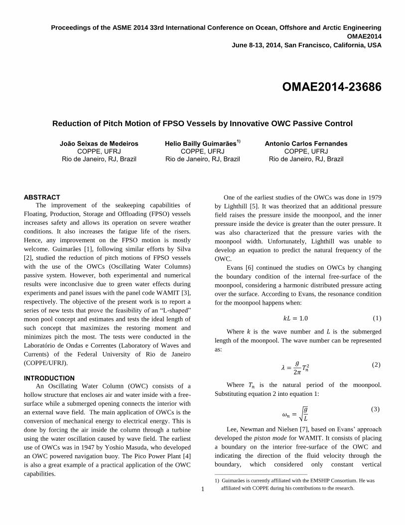
The first approach was to analyze the water flow through

the Reynolds Transport Theorem [9]. The control volume is

represented in Fig. 1 and, considering that the cross-section

remains constant:

(4)

The Transport Theorem states that:

∑ ∬ ( )

(5)

Figure 2 - (a) Control Volume, (b) Reference System

The horizontal and vertical forces are, respectively:

( ) (6)

(7)

It is then clear that the force , which is responsible for

the Restoring Moment desired, is maximized if .

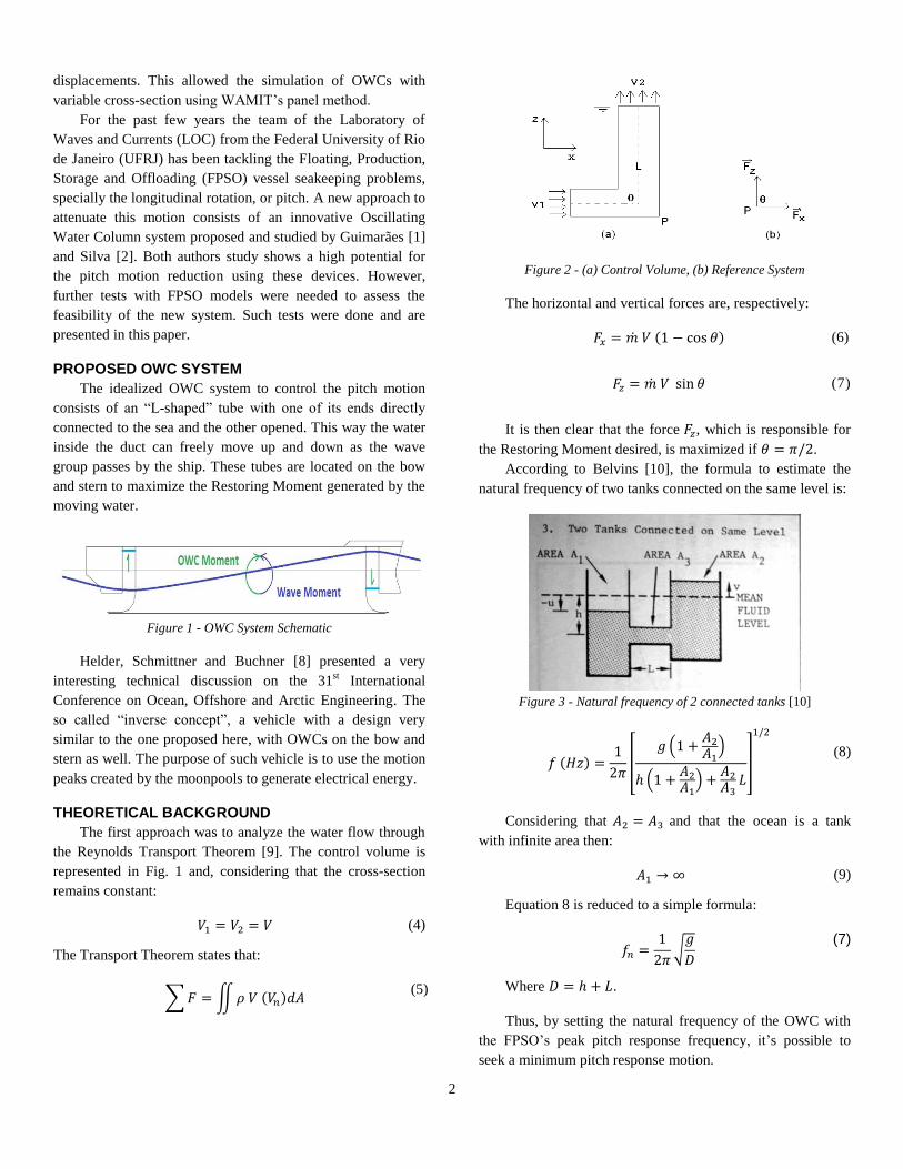
According to Belvins [10], the formula to estimate the

natural frequency of two tanks connected on the same level is:

Figure 3 - Natural frequency of 2 connected tanks [10]

( )

[

( )

( )

]

(8)

Considering that and that the ocean is a tank

with infinite area then:

(9)

Equation 8 is reduced to a simple formula:

√

(7)

Where .

Thus, by setting the natural frequency of the OWC with

the FPSO’s peak pitch response frequency, it’s possible to

seek a minimum pitch response motion.

3

DYNAMIC VIBRATION ABSORBER

The OWCs influence over the FPSO pitch motion can be

predicted by considering the first as a dynamic absorber

attached to the primary system that is the vessel.

Consider a non-damped vibration system with one degree

of freedom, mass and stiffness , subjected to a harmonic

excitation of frequency . Attached to this system is a

secondary one of mass and stiffness , also with one

degree of freedom that will work as a dynamic vibration

absorber (Fig. 4).

Figure 4 – Dynamic vibration absorber attached to the primary

system (no damping)

The equations of motion can be written as:

[ ] { ( )} [ ] { ( )} { ( )} (10)

Where:

Writing the equations of motion in the frequency domain,

the Frequency Response Functions are obtained:

( )

( )(

)

(11)

( )

(

)( )

(12)

If √

then equation 11 states that the Frequency

Response Function for the primary system will always be zero

regardless of the force F acting on the system. There is then an

anti-resonance condition for the primary system. The

frequency that causes this condition is the natural frequency of

the Dynamic Vibration Absorber (DVA).

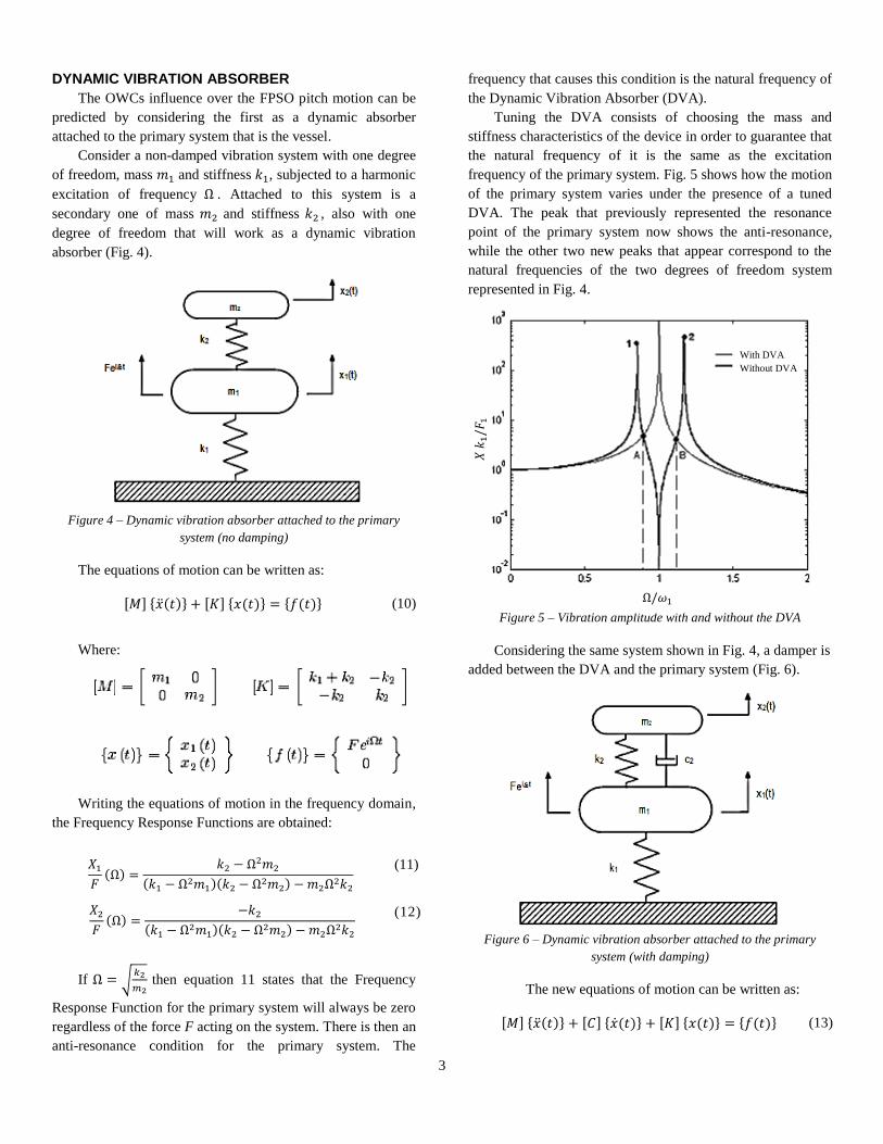
Tuning the DVA consists of choosing the mass and

stiffness characteristics of the device in order to guarantee that

the natural frequency of it is the same as the excitation

frequency of the primary system. Fig. 5 shows how the motion

of the primary system varies under the presence of a tuned

DVA. The peak that previously represented the resonance

point of the primary system now shows the anti-resonance,

while the other two new peaks that appear correspond to the

natural frequencies of the two degrees of freedom system

represented in Fig. 4.

Figure 5 – Vibration amplitude with and without the DVA

Considering the same system shown in Fig. 4, a damper is

added between the DVA and the primary system (Fig. 6).

Figure 6 – Dynamic vibration absorber attached to the primary

system (with damping)

The new equations of motion can be written as:

[ ] { ( )} [ ] { ( )} [ ] { ( )} { ( )} (13)

𝑋 𝑘 𝐹

With DVA

Without DVA

4

Where:

It’s important to notice the influence of the tuning factor

. Fig. 7 shows how the tuning factor affects the

motion peaks and their position, as increases the low

frequency peak increases while the other decreases.

Figure 7 – Tuning Factor influence

The damping factor ( ) plays a big role in the motion as

well. As increases the two peaks decrease and the motion

curve flattens out.

Figure 8 – Damping factor influence over the motion

An optimized DVA, as proposed by Den Hartog [11], is

based on the determination of the values of and so that the

points P and Q are on the same height and the highest peak

passes through one of them. These criteria will always ensure

that the response of the primary system will be as flat as

possible (Fig. 9).

Figure 9 – Comparison between optimized DVA, non-optimized DVA

and the primary system motion without the absorber

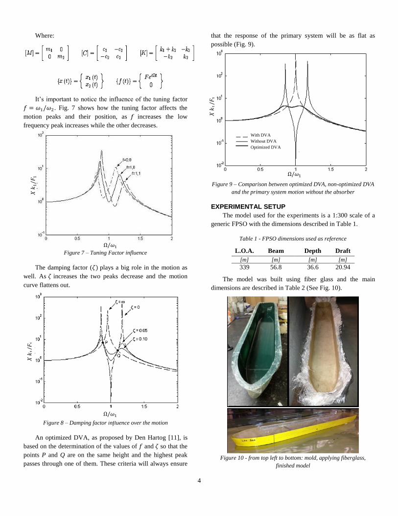
EXPERIMENTAL SETUP

The model used for the experiments is a 1:300 scale of a

generic FPSO with the dimensions described in Table 1.

Table 1 - FPSO dimensions used as reference

L.O.A. Beam Depth Draft

[m] [m] [m] [m]

339 56.8 36.6 20.94

The model was built using fiber glass and the main

dimensions are described in Table 2 (See Fig. 10).

Figure 10 - from top left to bottom: mold, applying fiberglass,

finished model

𝑋 𝑘 𝐹

𝑋 𝑘 𝐹

𝑋 𝑘 𝐹

With DVA

Without DVA

Optimized DVA

5

Table 2 - Main dimensions of the model

L.O.A. Beam Depth Draft L.C.G. Mass

[m] [m] [m] [m] [m] [kg]

1.13 0.17 0.122 0.069 0.575 11.52

Pitch Inertia

[kg*m2]

1.152

The main dimensions were set by the geometry itself, but

the longitudinal center of Gravity (L.C.G.), the mass and the

pitch inertia was properly set by placing weights inside. This

was done with two bifilar tests as described in the annex

section. The final pitch inertia and L.C.G. calculated for the

model was:

Inertia LCG

[kg m²] [m]

Model 1.225 0.57

Objective 1.152 0.57

Difference 6% 0%

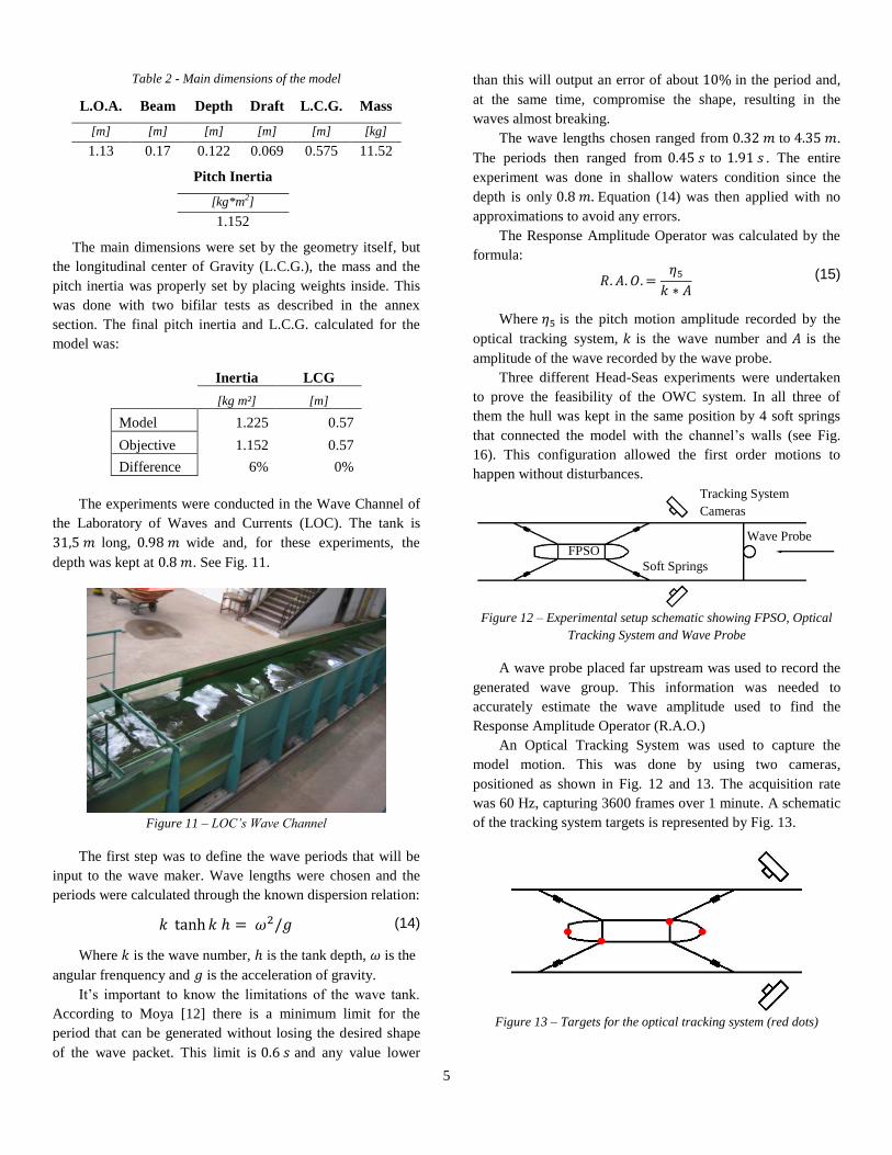
The experiments were conducted in the Wave Channel of

the Laboratory of Waves and Currents (LOC). The tank is

long, wide and, for these experiments, the

depth was kept at . See Fig. 11.

Figure 11 – LOC’s Wave Channel

The first step was to define the wave periods that will be

input to the wave maker. Wave lengths were chosen and the

periods were calculated through the known dispersion relation:

(14)

Where is the wave number, is the tank depth, is the

angular frenquency and is the acceleration of gravity.

It’s important to know the limitations of the wave tank.

According to Moya [12] there is a minimum limit for the

period that can be generated without losing the desired shape

of the wave packet. This limit is and any value lower

than this will output an error of about in the period and,

at the same time, compromise the shape, resulting in the

waves almost breaking.

The wave lengths chosen ranged from to .

The periods then ranged from to . The entire

experiment was done in shallow waters condition since the

depth is only Equation (14) was then applied with no

approximations to avoid any errors.

The Response Amplitude Operator was calculated by the

formula:

(15)

Where is the pitch motion amplitude recorded by the

optical tracking system, is the wave number and is the

amplitude of the wave recorded by the wave probe.

Three different Head-Seas experiments were undertaken

to prove the feasibility of the OWC system. In all three of

them the hull was kept in the same position by 4 soft springs

that connected the model with the channel’s walls (see Fig.

16). This configuration allowed the first order motions to

happen without disturbances.

Figure 12 – Experimental setup schematic showing FPSO, Optical

Tracking System and Wave Probe

A wave probe placed far upstream was used to record the

generated wave group. This information was needed to

accurately estimate the wave amplitude used to find the

Response Amplitude Operator (R.A.O.)

An Optical Tracking System was used to capture the

model motion. This was done by using two cameras,

positioned as shown in Fig. 12 and 13. The acquisition rate

was 60 Hz, capturing 3600 frames over 1 minute. A schematic

of the tracking system targets is represented by Fig. 13.

Figure 13 – Targets for the optical tracking system (red dots)

FPSO

Tracking System

Cameras

Wave Probe

Soft Springs

6

Finally, due to the channel characteristics, some reflected

waves from the wall were observed during the experiments.

The energy carried by those waves will be “trapped” near the

model without dissipating. However, this won’t compromise

the results, since a comparative analysis will be done to prove

the feasibility of the OWC and all three tests are going to be

subject to the same wall reflection.

WAMIT

Guimarães [1] used the approximations proposed by

Bhattacharyya [13] to estimate the radius of gyration to be

input into WAMIT, which was equivalent to the inertia in

Table 1. The FPSO with the dimensions described in Table 1

was then subdivided into patches using Rhinoceros (Fig. 14).

Figure 14 - FPSO panels for WAMIT (Rhinoceros)

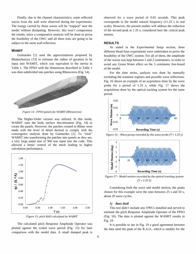
The Higher-Order version was utilized. In this mode,

WAMIT uses the body surface discretization (Fig. 14) to

create the panels. However, the patches created in Rhino were

made with the level of detail desired to comply with the

convergence analysis done by Guimarães [1]. To “trick”

WAMIT into transforming the patches into panels as they are,

a very large panel size of 300 was input into the code. This

allowed a better control of the mesh leading to higher

calculation performance.

Figure 15- pitch RAO calculated by WAMIT

The calculated pitch Response Amplitude Operator was

plotted against the scaled wave period (Fig. 15) for later

comparison with the model data. A small damped peak is

observed for a wave period of 0.65 seconds. This peak

corresponds to the model natural frequency (11.25 s in real

scale). However, the present studies will address the reduction

of the second peak at 1.35 s, considered here the critical peak

motion.

RESULTS

As stated in the Experimental Setup section, three

different Head-Seas experiments were undertaken to prove the

feasibility of the OWC system. For all of them, the amplitude

of the waves was kept between 1 and 2 centimeters, in order to

avoid any Green Water effect on the 5 centimeter free-board

of the model.

For the time series, analysis was done by manually

excluding the transient regimes and possible wave reflections.

Fig. 16 shows an example of an acquisition done by the wave

probe for a period of 1.35 s, while Fig. 17 shows the

acquisitions done by the optical tracking system for the same

period.

Figure 16 – Wave group recorded by the wave probe (T = 1.35 s)

Figure 17 – Model motion recorded by the optical tracking system

(T = 1.35 S)

Considering both the wave and model motion, the peaks

chosen for this example were the ones between 25 s and 50 s,

about 20 wave cycles.

1) Bare Hull

This test didn’t include any OWCs installed and served to

estimate the pitch Response Amplitude Operator of the FPSO

(Fig. 10). The data is plotted against the WAMIT results in

Fig. 19.

It is possible to see in Fig. 19 a good agreement between

the data until the peak of the R.A.O., which is smaller for the

0.00

0.20

0.40

0.60

0.80

1.00

1.20

1.40

0.00 0.50 1.00 1.50 2.00 2.50

η5

/ (k

*A

)

T (s)

-0.02

-0.01

0

0.01

0.02

0 10 20 30 40 50 60

Wave

Moti

on

(m

)

Recording Time (s)

-3

-2

-1

0

1

2

3

0 10 20 30 40 50 60

Mod

el M

oti

on

(d

eg)

Recording Time (s)

7

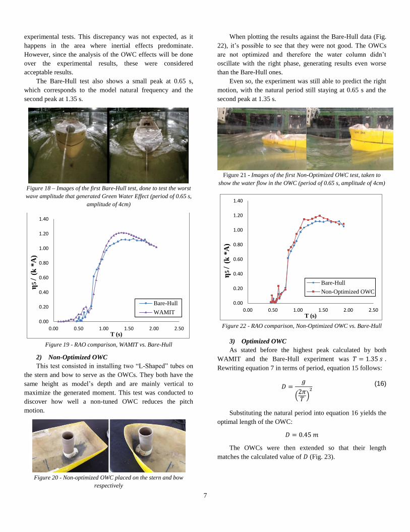
experimental tests. This discrepancy was not expected, as it

happens in the area where inertial effects predominate.

However, since the analysis of the OWC effects will be done

over the experimental results, these were considered

acceptable results.

The Bare-Hull test also shows a small peak at 0.65 s,

which corresponds to the model natural frequency and the

second peak at 1.35 s.

Figure 18 – Images of the first Bare-Hull test, done to test the worst

wave amplitude that generated Green Water Effect (period of 0.65 s,

amplitude of 4cm)

Figure 19 - RAO comparison, WAMIT vs. Bare-Hull

2) Non-Optimized OWC

This test consisted in installing two “L-Shaped” tubes on

the stern and bow to serve as the OWCs. They both have the

same height as model’s depth and are mainly vertical to

maximize the generated moment. This test was conducted to

discover how well a non-tuned OWC reduces the pitch

motion.

Figure 20 - Non-optimized OWC placed on the stern and bow

respectively

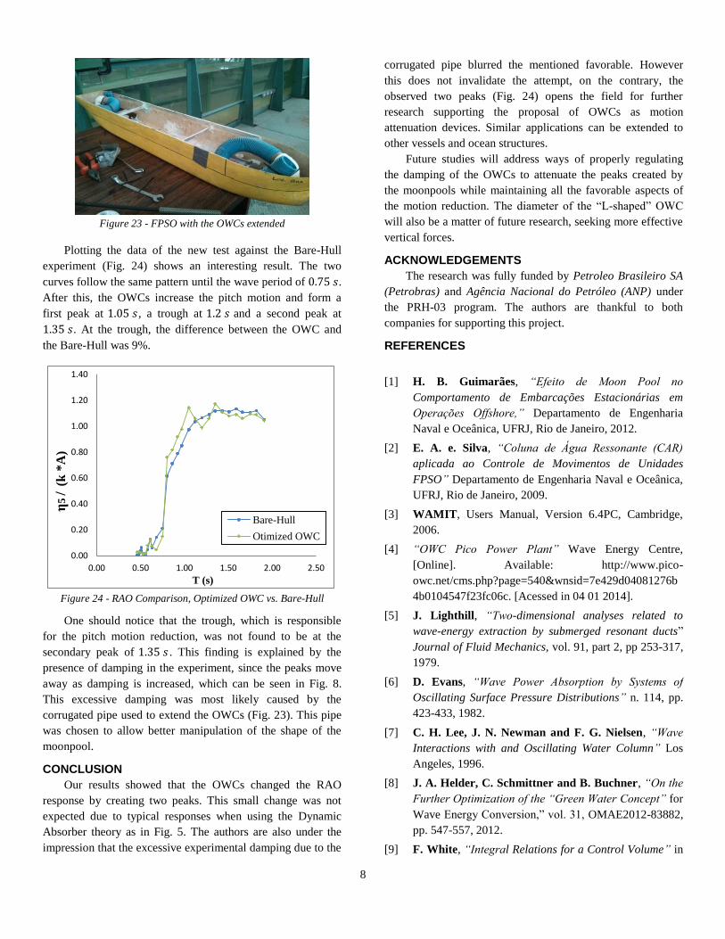
When plotting the results against the Bare-Hull data (Fig.

22), it’s possible to see that they were not good. The OWCs

are not optimized and therefore the water column didn’t

oscillate with the right phase, generating results even worse

than the Bare-Hull ones.

Even so, the experiment was still able to predict the right

motion, with the natural period still staying at 0.65 s and the

second peak at 1.35 s.

Figure 21 - Images of the first Non-Optimized OWC test, taken to

show the water flow in the OWC (period of 0.65 s, amplitude of 4cm)

Figure 22 - RAO comparison, Non-Optimized OWC vs. Bare-Hull

3) Optimized OWC

As stated before the highest peak calculated by both

WAMIT and the Bare-Hull experiment was .

Rewriting equation 7 in terms of period, equation 15 follows:

( )

(16)

Substituting the natural period into equation 16 yields the

optimal length of the OWC:

The OWCs were then extended so that their length

matches the calculated value of (Fig. 23).

0.00

0.20

0.40

0.60

0.80

1.00

1.20

1.40

0.00 0.50 1.00 1.50 2.00 2.50

η5

/ (k

*A

)

T (s)

Bare-Hull

WAMIT

0.00

0.20

0.40

0.60

0.80

1.00

1.20

1.40

0.00 0.50 1.00 1.50 2.00 2.50

η5

/ (k

*A

)

T (s)

Bare-Hull

Non-Optimized OWC

8

Figure 23 - FPSO with the OWCs extended

Plotting the data of the new test against the Bare-Hull

experiment (Fig. 24) shows an interesting result. The two

curves follow the same pattern until the wave period of .

After this, the OWCs increase the pitch motion and form a

first peak at , a trough at and a second peak at

. At the trough, the difference between the OWC and

the Bare-Hull was 9%.

Figure 24 - RAO Comparison, Optimized OWC vs. Bare-Hull

One should notice that the trough, which is responsible

for the pitch motion reduction, was not found to be at the

secondary peak of . This finding is explained by the

presence of damping in the experiment, since the peaks move

away as damping is increased, which can be seen in Fig. 8.

This excessive damping was most likely caused by the

corrugated pipe used to extend the OWCs (Fig. 23). This pipe

was chosen to allow better manipulation of the shape of the

moonpool.

CONCLUSION

Our results showed that the OWCs changed the RAO

response by creating two peaks. This small change was not

expected due to typical responses when using the Dynamic

Absorber theory as in Fig. 5. The authors are also under the

impression that the excessive experimental damping due to the

corrugated pipe blurred the mentioned favorable. However

this does not invalidate the attempt, on the contrary, the

observed two peaks (Fig. 24) opens the field for further

research supporting the proposal of OWCs as motion

attenuation devices. Similar applications can be extended to

other vessels and ocean structures.

Future studies will address ways of properly regulating

the damping of the OWCs to attenuate the peaks created by

the moonpools while maintaining all the favorable aspects of

the motion reduction. The diameter of the “L-shaped” OWC

will also be a matter of future research, seeking more effective

vertical forces.

ACKNOWLEDGEMENTS

The research was fully funded by Petroleo Brasileiro SA

(Petrobras) and Agência Nacional do Petróleo (ANP) under

the PRH-03 program. The authors are thankful to both

companies for supporting this project.

REFERENCES

[1] H. B. Guimarães, “Efeito de Moon Pool no

Comportamento de Embarcações Estacionárias em

Operações Offshore,” Departamento de Engenharia

Naval e Oceânica, UFRJ, Rio de Janeiro, 2012.

[2] E. A. e. Silva, “Coluna de Água Ressonante (CAR)

aplicada ao Controle de Movimentos de Unidades

FPSO” Departamento de Engenharia Naval e Oceânica,

UFRJ, Rio de Janeiro, 2009.

[3] WAMIT, Users Manual, Version 6.4PC, Cambridge,

2006.

[4] “OWC Pico Power Plant” Wave Energy Centre,

[Online]. Available: http://www.pico-

owc.net/cms.php?page=540&wnsid=7e429d04081276b

4b0104547f23fc06c. [Acessed in 04 01 2014].

[5] J. Lighthill, “Two-dimensional analyses related to

wave-energy extraction by submerged resonant ducts”

Journal of Fluid Mechanics, vol. 91, part 2, pp 253-317,

1979.

[6] D. Evans, “Wave Power Absorption by Systems of

Oscillating Surface Pressure Distributions” n. 114, pp.

423-433, 1982.

[7] C. H. Lee, J. N. Newman and F. G. Nielsen, “Wave

Interactions with and Oscillating Water Column” Los

Angeles, 1996.

[8] J. A. Helder, C. Schmittner and B. Buchner, “On the

Further Optimization of the “Green Water Concept” for

Wave Energy Conversion,” vol. 31, OMAE2012-83882,

pp. 547-557, 2012.

[9] F. White, “Integral Relations for a Control Volume” in

0.00

0.20

0.40

0.60

0.80

1.00

1.20

1.40

0.00 0.50 1.00 1.50 2.00 2.50

η5

/ (k

*A

)

T (s)

Bare-Hull

Otimized OWC

9

Fluid Mechanics 4th Ed., University of Rhode Island,

McGraw-Hill, 1999, pp. 215 - 274.

[10] R. D. Belvins, "Formulas for Natural Frequency and

Mode Shape", Litton Educational Publishing Inc., 1979.

[11] D. Hartog, “Mechanical Vibrations” Mineola, Dover

Publications Inc., pp. 87-102.

[12] M. A. Moya, “Development and Implementation of

Worst Sea - Best Sea (WS/BS) Method for Mooring

Structures - Ms.C. Thesis” COPPE, UFRJ, Rio de

Janeiro, Brazil, 2013.

[13] R. Bhattacharyya, "Dynamics of Marine Vehicles",

New York: John Wiley and Sons Inc., 1978.

ANNEX

a) First Bifilar Test

To calculate the inertia of the bare model, a simple bifilar

test was conducted (Fig. 25). For this the scaled FPSO was

hung from its side so that the longitudinal axis was

perpendicular to the lines holding it. The two lines were

equidistant from the center of gravity.

The vessel was then forced to oscillate under small

amplitudes of motion, and the period of oscillation (T) was

then recorded for three different distances from the pivot

point.

Figure 25 - Mass moment of inertia test schematic

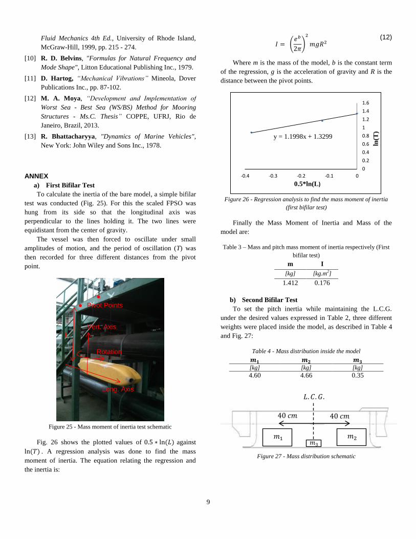
Fig. 26 shows the plotted values of ( ) against

( ) . A regression analysis was done to find the mass

moment of inertia. The equation relating the regression and

the inertia is:

(

)

(12)

Where m is the mass of the model, b is the constant term

of the regression, g is the acceleration of gravity and R is the

distance between the pivot points.

Figure 26 - Regression analysis to find the mass moment of inertia

(first bifilar test)

Finally the Mass Moment of Inertia and Mass of the

model are:

Table 3 – Mass and pitch mass moment of inertia respectively (First

bifilar test)

m I

[kg] [kg.m2]

1.412 0.176

b) Second Bifilar Test

To set the pitch inertia while maintaining the L.C.G.

under the desired values expressed in Table 2, three different

weights were placed inside the model, as described in Table 4

and Fig. 27:

Table 4 - Mass distribution inside the model

[kg] [kg] [kg]

4.60 4.66 0.35

Figure 27 - Mass distribution schematic

y = 1.1998x + 1.3299

0

0.2

0.4

0.6

0.8

1

1.2

1.4

1.6

-0.4 -0.3 -0.2 -0.1 0

ln(T

)

0.5*ln(L)

𝑚 𝑚 𝑚

𝑐𝑚 𝑐𝑚

𝐿 𝐶 𝐺 Long. Axis

Vert. Axis

Rotation

Pivot Points

L

10

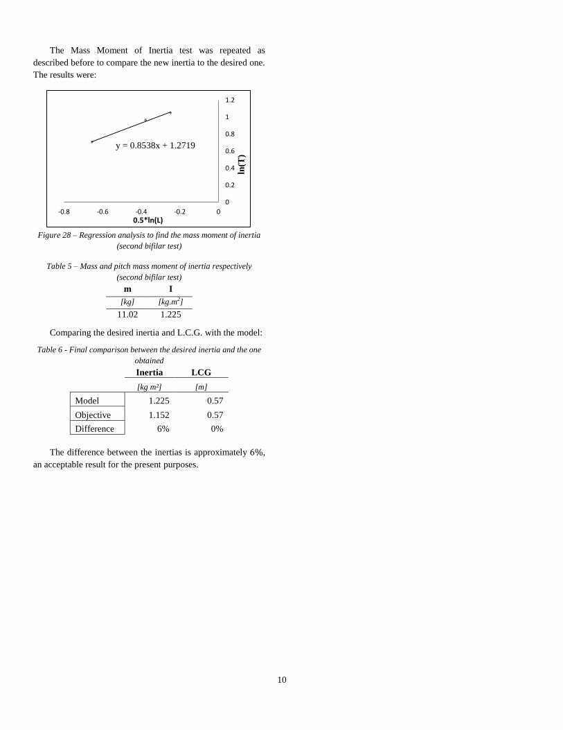
The Mass Moment of Inertia test was repeated as

described before to compare the new inertia to the desired one.

The results were:

Figure 28 – Regression analysis to find the mass moment of inertia

(second bifilar test)

Table 5 – Mass and pitch mass moment of inertia respectively

(second bifilar test)

m I

[kg] [kg.m2]

11.02 1.225

Comparing the desired inertia and L.C.G. with the model:

Table 6 - Final comparison between the desired inertia and the one

obtained

Inertia LCG

[kg m²] [m]

Model 1.225 0.57

Objective 1.152 0.57

Difference 6% 0%

The difference between the inertias is approximately ,

an acceptable result for the present purposes.

y = 0.8538x + 1.2719

0

0.2

0.4

0.6

0.8

1

1.2

-0.8 -0.6 -0.4 -0.2 0

ln(T

)

0.5*ln(L)