Offprint CPC2012

This article appeared in a journal published by Elsevier. The attachedcopy is furnished to the author for internal non-commercial researchand education use, including for instruction at the authors institution

and sharing with colleagues.

Other uses, including reproduction and distribution, or selling orlicensing copies, or posting to personal, institutional or third party

websites are prohibited.

In most cases authors are permitted to post their version of thearticle (e.g. in Word or Tex form) to their personal website orinstitutional repository. Authors requiring further information

regarding Elsevier’s archiving and manuscript policies areencouraged to visit:

http://www.elsevier.com/copyright

http://www.elsevier.com/copyright

Author's personal copy

Computer Physics Communications 183 (2012) 552–569

Contents lists available at SciVerse ScienceDirect

Computer Physics Communications

www.elsevier.com/locate/cpc

Fourth-order compact difference and alternating direction implicit schemes fortelegraph equations

Shu-Sen Xie a,1, Su-Cheol Yi b,∗,2, Tae In Kwon b

a School of Mathematical Sciences, Ocean University of China, Qingdao 266100, PR Chinab Department of Mathematics, Changwon National University, Changwon, 641-773, Republic of Korea

a r t i c l e i n f o a b s t r a c t

Article history:Received 9 August 2010Received in revised form 18 November 2011Accepted 29 November 2011Available online 1 December 2011

Keywords:Telegraph equationCompact difference schemeAlternating direction implicit schemeStabilityError estimate

In this paper, two- and three-level compact difference and alternating direction implicit schemes arepresented for the numerical solutions of one- and two-dimensional linear telegraph equations andtelegraph equations with nonlinear forcing term. The stability and error estimates are given. Theconvergence rates of the present schemes are of order O(τ 2 + h4). Numerical experiments on modelproblems show that the present schemes are of high accuracy.

© 2011 Elsevier B.V. All rights reserved.

1. Introduction

The telegraph equation is one of the important equations ofmathematical physics with applications in many different fieldssuch as transmission and propagation of electrical signals [1,2],vibrational systems [3], random walk theory [4], and mechanicalsystems [5], etc. The heat diffusion and wave propagation equa-tions are particular cases of the telegraph equation.

Recently, increasing attention has been paid to the develop-ment, analysis, and implementation of stable methods for the nu-merical solutions of second-order hyperbolic equations. There havebeen many numerical methods for hyperbolic equations, such asthe finite difference, the finite element, and the collocation meth-ods, etc. See [6–21] and literatures are therein. Mohanty et al.[17,18] developed some alternating direction implicit schemes forthe two- and three-dimensional linear hyperbolic equations. Mostof these schemes are second-order accurate in both space andtime. Some conditionally stable fourth-order compact differenceschemes for the wave and telegraph equations were introduced in[8,9,13]. An advantage of compact difference schemes is that theschemes use narrower stencils, i.e., fewer neighboring nodes, and

* Corresponding author.E-mail addresses: [email protected] (S.-S. Xie), [email protected]

(S.-C. Yi), [email protected] (T.I. Kwon).1 The research of this author is partially supported by NNSF of China grants

10971204.2 The research of this author was supported by Changwon National University in

2009.

have less truncation error comparing to typical finite differenceschemes. Various versions of compact schemes have been suc-cessfully developed and analyzed (cf. [22,23]) and references aretherein. The alternating direction implicit (ADI) methods were firstintroduced by Douglas, Peaceman, and Rachford [24–27], whichhave an advantage of no increase in dimension of the coefficientmatrices corresponding matrix equations. There are many exten-sions and a great variety of applications of ADI based on the finitedifference or the finite element methods [28–33].

In this paper, we propose two- and three-level compact dif-ference and ADI compact difference schemes with high accuracyfor numerical solutions of the one- and two-dimensional tele-graph equations with Dirichlet boundary conditions. These com-pact schemes are unconditionally stable and have a truncation er-ror of second- and fourth-order in time and space, respectively.The coefficient matrices of the matrix equations given by theschemes are symmetric and tridiagonal. The matrix equations canbe effectively solved by using many linear solvers. Numerical ex-periments presented for the 1D and 2D telegraph equations showthat the present schemes are of high accuracy. By comparing thenumerical results obtained by the present methods with the onesof some other available methods, the present methods can be con-sidered as practical and effective numerical techniques to solvetelegraph equations.

In Section 2, we introduce the compact difference schemes forthe 1D telegraph equation and consider the stability and error es-timates of the schemes. In Section 3, we introduce the compactdifference and ADI compact difference schemes for the 2D tele-graph equation, and analyze the stabilities and error estimates of

0010-4655/$ – see front matter © 2011 Elsevier B.V. All rights reserved.doi:10.1016/j.cpc.2011.11.023


S.-S. Xie et al. / Computer Physics Communications 183 (2012) 552–569 553

the schemes. Finally, we present the result of numerical experi-ments on test examples in Section 4.

2. One-dimensional telegraph equation

Let I = (0, X). Consider the 1D linear telegraph equation

∂2u

∂t2+ c

∂u

∂t+ bu − p

∂2u

∂x2= f (x, t), (x, t) ∈ I × (0, T ], (1)

with the initial and boundary conditions

u(x,0) = ϕ(x),∂u

∂t(x,0) = ψ(x),

u(0, t) = gl(t), u(X, t) = gr(t),

where c, b, and p are constants with c, b � 0, and p > 0, and thefunctions f , ϕ , and ψ are assumed to be sufficiently smooth.

2.1. The fourth-order compact difference schemes

The solution domain Ω = {(x, t) | 0 � x � X, 0 � t � T } is dis-cretized into grids described by the set {(x j, tn)} of nodes, in whichx j = jh, j = 0,1, . . . , J and tn = nτ , n = 0,1, . . . , N = T /τ , whereh and τ are the discretization parameters. Let un

j = u(x j, tn) andlet Ih = {x0, x1, . . . , x J } denote the set of nodes of the intervalI = [0, X]. We use the following difference operators for simplic-ity:

∂tt unj = un+1

j − 2unj + un−1

j

τ 2, ∂t un

j = un+1j − un−1

j

2τ,

∂t unj = un+1

j − unj

τ, ∂xun

j = unj+1 − un

j

h,

∂xunj = un

j − unj−1

h,

δ2x un

j = ∂xunj − ∂xun

j

h= un

j+1 − 2unj + un

j−1

h2,

un+ 1

2j = 1

2

(un+1

j + unj

).

Setting w = p ∂2u∂x2 , the equation in (1) can be written as

w = ∂2u

∂t2+ c

∂u

∂t+ bu − f . (2)

Let Lx = 1 + h2

12 δ2x . By using a Taylor expansion, we get

Lx wnj = pδ2

x unj + O(h4). (3)

Substituting (2) into (3) and using a popular three-level time dis-cretization, we have

Lx(∂tt un

j + c∂t unj + b

(θun+1

j + (1 − 2θ)unj + θun−1

j

))− Lx

(θ f n+1

j + (1 − 2θ) f nj + θ f n−1

j

)= pδ2

x

(θun+1

j + (1 − 2θ)unj + θun−1

j

)+ O(τ 2 + h4), (4)

where θ ∈ [0,1/2] is a parameter.Let Un

j denote the approximation of unj , Un

θ, j = θUn+1j + (1 −

2θ)Unj + θUn−1

j , and let f nθ, j = θ f n+1

j + (1 − 2θ) f nj + θ f n−1

j . From(4) we obtain the following three-level compact difference scheme,which has a truncation error of order O(τ 2 + h4):⎧⎪⎪⎪⎨⎪⎪⎪⎩

Lx(∂tt Un

j + c∂t Unj + bUn

θ, j

)− p δ2x Un

θ, j = Lx f nθ, j,

1 � j � J − 1, 1 � n � N − 1,

Un0 = gn

l , UnJ = gn

r , 0 � n � N,

U 0j = ϕ j, 0 � j � J .

(5)

To implement the scheme above, the first approximation U 1j

should be prescribed accurately and it can be evaluated in the fol-lowing manner:

Since

u(x, τ ) = ϕ(x) + τψ(x) + τ 2

2

∂2u

∂t2(x,0) + O(τ 3),

and

∂2u

∂t2= −c

∂u

∂t− bu + p

∂2u

∂x2+ f ,

we get

u(x, τ ) =(

1 − τ 2b

2

)ϕ +

(τ − τ 2c

2

)ψ

+ τ 2

2

(pϕ′′ + f (x,0)

)+ O(τ 3),where ϕ′′ denotes the second-order derivative of ϕ . Thus, u1

j canbe approximated by

U 1j =

(1 − τ 2b

2

)ϕ j +

(τ − τ 2c

2

)ψ j + τ 2

2

(pδ2

x ϕ j + f 0j

), (6)

or

LxU 1j = τ 2

2pδ2

x ϕ j + Lx(ϕ j + τψ j)

− τ 2

2Lx(bϕ j + cψ j − f 0

j

). (7)

The approximations in (6) and (7) have truncation errors of orderO(τ 2h2 + τ 3) and O(τ 2h4 + τ 3), respectively. By introducing theauxiliary variable v = ∂u

∂t , we can derive the following two-levelCrank–Nicolson compact difference scheme:

Setting w = p ∂2u∂x2 , the equation in (1) can be written as

w = ∂v

∂t+ c

∂u

∂t+ bu − f .

By using a Taylor expansion, we get vn+ 1

2j = ∂t un

j + O(τ 2) and

wn+ 1

2j = ∂t vn

j + c∂t unj + bu

n+ 12

j − fn+ 1

2j + O(τ 2). (8)

Substituting (8) into (3), we have

Lx(∂t vn

j + c∂t unj + bu

n+ 12

j − fn+ 1

2j

)= pδ2x u

n+ 12

j + O(τ 2 + h4).Let Un

j and V nj denote the approximations of un

j and vnj , re-

spectively. We then obtain the following two-level compact differ-ence scheme and this scheme has also a truncation error of orderO(τ 2 + h4).⎧⎪⎪⎪⎪⎪⎪⎪⎪⎪⎪⎪⎪⎪⎪⎪⎨⎪⎪⎪⎪⎪⎪⎪⎪⎪⎪⎪⎪⎪⎪⎪⎩

Lx(∂t V n

j + c∂t Unj + bU

n+ 12

j

)− pδ2x U

n+ 12

j = Lx fn+ 1

2j ,

∂t Unj = V

n+ 12

j , 1 � j � J − 1, 0 � n � N − 1,

V n+10 = 2

τ

(gn+1

l − gnl

)− V n0 ,

V n+1J = 2

τ

(gn+1

r − gnr

)− V nJ ,

Un+10 = gn+1

l , Un+1J = gn+1

r , 0 � n � N − 1,

U 0j = ϕ j, V 0

j = ψ j, 0 � j � J .

(9)

We now show the equivalence of the two- and three-level com-pact difference schemes for a particular value of θ . By summingthe first equations in (9) with n = k − 1 and k, we obtain


554 S.-S. Xie et al. / Computer Physics Communications 183 (2012) 552–569

Lx

(∂t V k

j + c∂t Ukj + 1

4b(Uk+1

j + 2Ukj + Uk−1

j

))− p

4δ2

x

(Uk+1

j + 2Ukj + Uk−1

j

)= 1

4Lx(

f k+1j + 2 f k

j + f k−1j

). (10)

Considering the second equations in (9) with n = k − 1 and k, weget ∂t V k

j = ∂tt U kj , and, hence, (10) shows that the two-level scheme

(9) is equivalent to the three-level scheme (5) with θ = 1/4.Consider the 1D telegraph equation with nonlinear forcing term⎧⎪⎪⎪⎪⎨⎪⎪⎪⎪⎩∂2u

∂t2+ c

∂u

∂t− p

∂2u

∂x2= f (x, u), (x, t) ∈ I × (0, T ],

u(x,0) = ϕ(x),∂u

∂t(x,0) = ψ(x),

u(0, t) = gl(t), u(X, t) = gr(t).

(11)

By using a similar argument as the one used for the 1D lineartelegraph equation, we can derive the following three- and two-level compact difference schemes (12) and (13), respectively, forproblem (11). These schemes also have a truncation error of orderO(τ 2 + h4).⎧⎪⎪⎪⎪⎨⎪⎪⎪⎪⎩

Lx(∂tt Un

j + c∂t Unj

)− pδ2x Un

θ, j = Lx f nj ,

1 � j � J − 1, 1 � n � N − 1,

Un0 = gn

l , UnJ = gn

r , 0 � n � N,

U 0j = ϕ j, 0 � j � J ,

(12)

where f nj = f (x j, Un

j ). The first approximation U 1j in (12) can be

computed as

U 1j = ϕ j +

(τ − τ 2c

2

)ψ j + τ 2

2

(pδ2

x ϕ j + f (x j,ϕ j)),

or

LxU 1j = τ 2

2pδ2

x ϕ j + Lx(ϕ j + τψ j) − τ 2

2Lx(cψ j − f (x j,ϕ j)

).

⎧⎪⎪⎪⎪⎪⎪⎪⎪⎪⎪⎪⎪⎪⎪⎪⎪⎪⎪⎪⎨⎪⎪⎪⎪⎪⎪⎪⎪⎪⎪⎪⎪⎪⎪⎪⎪⎪⎪⎪⎩

Lx(∂t V 0

j + c∂t U 0j

)− pδ2x U

12j = Lx f

12j ,

Lx(∂t V n

j + c∂t Unj

)− pδ2x U

n+ 12

j = Lx( f E)nj , 1 � n � N − 1,

∂t Unj = V

n+ 12

j , 1 � j � J − 1, 0 � n � N − 1,

V n+10 = 2

τ

(gn+1

l − gnl

)− V n0 ,

V n+1J = 2

τ

(gn+1

r − gnr

)− V nJ ,

Un+10 = gn+1

l , Un+1J = gn+1

r , 0 � n � N − 1,

U 0j = ϕ j, V 0

j = ψ j, 0 � j � J ,

(13)

where f12j = f (x j, U

12j ) and ( f E )n

j = f (x j, (3Unj − Un−1

j )/2) is theextrapolation operator. For smooth function u(t), one can see that

un+ 12 − (3un − un−1)/2 = O(τ 2).

The first equation in (13) is implicit and nonlinear, and, hence,we will use the linear iterative algorithm to compute U 1

j :((4 + 2τ c)Lx − τ 2 pδ2

x

)U (s+1)

j

= ((4 + 2τ c)Lx + τ 2 pδ2x

)U 0

j + 4τLx V 0j + 2τ 2Lx f

(x j, W (s)

j

),

(14)

where s denotes the sth iteration, W (0)j = U 0

j , and W (s)j = (U (s)

j +U 0

j )/2 for s � 1. If ‖U (s+1) − U (s)‖L∞ < ε for some prescribed tol-

erance ε , we stop the iteration and set U 1j = U (s+1)

j . In general, acouple of iterations can reach a prescribed tolerance.

Let λ = τ/h, Un = (Un1, . . . , Un

J−1)T , V n = (V n

1 , . . . , V nJ−1)

T ,

F n = ( f n1 , . . . , f n

J−1)T , and let A and B denote the ( J − 1) × ( J − 1)

tridiagonal symmetric matrices given by

A =

⎛⎜⎜⎜⎜⎜⎜⎜⎝

10 1 0 . . . 0

1 10 1. . .

...

0. . .

. . .. . . 0

.... . . 1 10 1

0 . . . 0 1 10

⎞⎟⎟⎟⎟⎟⎟⎟⎠,

B =

⎛⎜⎜⎜⎜⎜⎜⎜⎝

−2 1 0 . . . 0

1 −2 1. . .

...

0. . .

. . .. . . 0

.... . . 1 −2 1

0 . . . 0 1 −2

⎞⎟⎟⎟⎟⎟⎟⎟⎠. (15)

Then schemes (5) and (9) can be written as the following linearmatrix equations, respectively:[α1A − 24θλ2 pB

]Un+1

= [α2A + 24(1 − 2θ)λ2 pB]Un

− [α3A − 24θλ2 pB]Un−1 + 2τ 2AF n

θ + Gn1,⎧⎪⎪⎪⎨⎪⎪⎪⎩

[γ1A − 6λ2 pB

]Un+1

= [γ2A + 6λ2 pB]Un + 2τAV n + τ 2AF n+ 1

2 + Gn2,

V n+1 = 2

τ

(Un+1 − Un)− V n,

where α1 = 2 + τ c + 2τ 2θb, α2 = 4 − 2τ 2(1 − 2θ)b, α3 = 2 − τ c +2τ 2θb, F n

θ = θ F n+1 + (1 − 2θ)F n + θ F n−1, γ1 = 2 + τ c + bτ 2/2,γ2 = 2 + τ c − bτ 2/2, and, Gn

1 and Gn2 are vectors corresponding

the boundary conditions.The compact difference schemes (12) and (13) also can be writ-

ten as matrix equations, which are similar to the ones above, by

replacing F nθ and F n+ 1

2 with F n and F nE , respectively, and setting

b = 0. One can see that schemes (5), (9), (12), and (13) give rise totridiagonal symmetric coefficient matrices corresponding the ma-trix equations, which can be easily solved by using effective linearsolvers.

2.2. Stability and error estimates

In the following analyses, we assume that the problem consid-ered has homogeneous boundary conditions for simplicity; that is,gl(t) = gr(t) = 0. Throughout this paper we will use M , with orwithout a subindex (subscript), as a generic positive constant notnecessarily the same at different occurrences.

Let H0(Ih) denote the set of grid functions u defined on Ih withu0 = u J = 0. We define the discrete inner products and norms onH0(Ih) by

(u, w) =J−1∑j=1

u j w jh, (u, w)l =J−1∑j=0

u j w jh,

‖u‖L2 =√(u, u), |||u|||L2 =√(u, u)l, |u|1 = |||∂xu|||L2 ,

‖u‖L∞ = max0� j� J

|u j|, ‖u‖21 = ‖u‖2

L2+ |u|21.



Lemma 2.1. For any grid function u defined on Ih and w ∈ H0(Ih), wehave(δ2

x u, w)= −(∂xu, ∂x w)l.

Proof.

(δ2

x u, w)=

J−1∑j=1

(∂xu j − ∂xu j−1)w j

hh

= −J−1∑j=0

∂xu j∂x w jh, since w0 = w J = 0

= −(∂xu, ∂x w)l. �Lemma 2.2. For all u ∈ H0(Ih), we have that

|u|21 � 4

h2‖u‖2

L2, ‖u‖2

L∞ � 1

h‖u‖2

L2.

Proof.

|u|21 = 1

h2

J−1∑j=0

(u2

j+1 − 2u ju j+1 + u2j

)h

� 1

h2

J−1∑j=0

(u2

j+1 + 2|u j||u j+1| + u2j

)h

� 2

h2

J−1∑j=0

(u2

j + u2j+1

)h = 4

h2‖u‖2

L2.

For each k, 1 � k � J − 1, we have

|uk|2 � 1

h

J−1∑j=1

|u j|2h = 1

h‖u‖2

L2.

This completes the proof. �Lemma 2.3. For all u ∈ H0(Ih), we have the inequalities

‖u‖L∞ �√

X

2|u|1, ‖u‖L2 � X

2|u|1.

Proof. For each k, 1 � k � J − 1, noting that u0 = 0, we have

|uk|2 =∣∣∣∣∣

k−1∑j=0

u j+1 − u j

hh

∣∣∣∣∣2

�(

k−1∑j=0

|∂xu j|h)2

� kh

(k−1∑j=0

|∂xu j|2h

)by Schwarz inequality. (16)

Similarly, we can get

|uk|2 � ( J − k)h

( J−1∑j=k

|∂xu j|2h

). (17)

Multiplying both sides of (16) and (17) by X − xk = ( J − k)h andxk = kh, respectively, and adding the inequalities side by side, weobtain

X |uk|2 � xk(X − xk)|||∂xu|||2L2� X2

4|u|21,

which implies ‖u‖L∞ �√

X2 |u|1 and ‖u‖2

L2=∑ J−1

k=1 |uk|2h � X2

4 |u|21.

This completes the proof. �We will show the stabilities and error estimates for the above

compact difference schemes. For this we will use the discrete ver-sion of Gronwall’s inequality, which is stated below:

Lemma 2.4. If {e j}∞j=0 is a sequence of nonnegative real numbers such

that en+1 � α + βτ∑n

j=0 e j , n � 0, where α � 0, β and τ are positiveconstants, then we have the inequality

en+1 � (α + βe0τ )eβ(n+1)τ .

Theorem 2.5. The compact difference scheme (5) is stable for θ ∈[1/4,1/2], and has the stability estimate

max0<n�N−1

{∥∥∂t Un∥∥2

L2+ bN n

θ (U ) +(

p − bh2

12

)En

θ (U )

}� M

{∥∥∂t U 0∥∥2

L2+ bN 0

θ (U ) + pE0θ (U ) + max

0�n�N

∥∥ f n∥∥2

L2

}, (18)

where

N nθ (U ) = θ

(∥∥Un+1∥∥2

L2+ ∥∥Un

∥∥2L2

)+ (1 − 2θ)(Un, Un+1)

= 1

2

(∥∥Un+1∥∥2

L2+ ∥∥Un

∥∥2L2

)− 1 − 2θ

2

∥∥Un+1 − Un∥∥2

L2� 0,

Enθ (U ) = θ

(∣∣Un+1∣∣21 + ∣∣Un

∣∣21

)+ (1 − 2θ)(∂xUn, ∂xUn+1)

l

= 1

2

(∣∣Un+1∣∣21 + ∣∣Un

∣∣21

)− 1 − 2θ

2

∣∣Un+1 − Un∣∣21 � 0.

Proof. By taking the inner product (·,·) on both sides of the firstequation in (5) with ∂t Un and using Lemma 2.1, we have

(∂tt Un + c∂t Un, ∂t Un)− h2

12

(∂tt∂xUn + c∂t∂xUn, ∂t∂xUn)

l

+ b(Un

θ , ∂t Un)− bh2

12

(∂xUn

θ , ∂t∂xUn)l + p

(∂xUn

θ , ∂t∂xUn)l

= ( f nθ , ∂t Un)− h2

12

(∂x f n

θ , ∂t∂xUn)l. (19)

It can be shown that

(∂tt Un + c∂t Un, ∂t Un)− h2

12

(∂tt∂xUn + c∂t∂xUn, ∂t∂xUn)

l

= 1

2τ

(∥∥∂t Un∥∥2

L2− h2

12

∣∣∂t Un∣∣21

)− 1

2τ

(∥∥∂t Un−1∥∥2

L2− h2

12

∣∣∂t Un−1∣∣21

)+ c∥∥∂t Un

∥∥2L2

− ch2

12

∣∣∂t Un∣∣21, (20)

b(Un

θ , ∂t Un)= θb(Un+1 + Un−1, ∂t Un)+ (1 − 2θ)b

(Un, ∂t Un)

= b

2τ

(N nθ (U ) − N n−1

θ (U )), (21)

(∂xUn

θ , ∂t∂xUn)l = 1

2τ

(Enθ (U ) − En−1

θ (U )). (22)

It is easy to see that N nθ (U ) � 0 and En

θ (U ) � 0 for θ ∈ [1/4,1/2]by simple calculation. By substituting (20)–(22) into (19) and sum-ming for n from 1 to k, 1 � k � N − 1, we get



∥∥∂t Uk∥∥2

L2− h2

12

∣∣∂t Uk∣∣21 + 2cτ

k∑n=1

(∥∥∂t Un∥∥2

L2− h2

12

∣∣∂t Un∣∣21

)

+ bN kθ (U ) +

(p − bh2

12

)Ek

θ (U )

�∥∥∂t U 0

∥∥2L2

− h2

12

∣∣∂t U 0∣∣21 + bN 0

θ (U ) +(

p − bh2

12

)E0

θ (U )

+ τ

k+1∑n=0

(∥∥ f n∥∥2

L2+ h2

12

∣∣ f n∣∣21

)

+ τ

k∑n=0

(∥∥∂t Un∥∥2

L2+ h2

12

∣∣∂t Un∣∣21

).

Using Lemma 2.2, we obtain

2

3

∥∥∂t Uk∥∥2

L2+ 4cτ

3

k∑n=1

∥∥∂t Un∥∥2

L2+ bN k

θ (U ) +(

p − bh2

12

)Ek

θ (U )

�∥∥∂t U 0

∥∥2L2

+ bN 0θ (U ) + p E0

θ (U )

+ 4τ

3

k+1∑n=0

∥∥ f n∥∥2

L2+ 4τ

3

k∑n=0

∥∥∂t Un∥∥2

L2. (23)

We then obtain (18) from the discrete Gronwall inequality by tak-ing h and τ sufficiently small. �

Since θ � 1/2, one can easily see that

N kθ (U ) = 1

2

(∥∥Uk+1∥∥2

L2+ ∥∥Uk

∥∥2L2

− (1 − 2θ)τ 2∥∥∂t Uk

∥∥2L2

)� 1

2

(∥∥Uk+1∥∥2

L2+ ∥∥Uk

∥∥2L2

),

Ekθ (U ) � 1

2

(∣∣Uk+1∣∣21 + ∣∣Uk

∣∣21

),

Ekθ (U ) = 1

2

(∣∣Uk+1∣∣21 + ∣∣Uk

∣∣21 − (1 − 2θ)τ 2

∣∣∂t Uk∣∣21

)� 1

2

(∣∣Uk+1∣∣21 + ∣∣Uk

∣∣21

)− 2(1 − 2θ)λ2∥∥∂t Uk

∥∥2L2

,

where λ = τ/h. Substituting the above estimates into (23) we ob-tain

1

3

(2 − b(1 − 2θ)τ 2 − 6p(1 − 2θ)λ2)∥∥∂t Uk

∥∥2L2

+ b

2

(∥∥Uk+1∥∥2

L2+ ∥∥Uk

∥∥2L2

)+ 12p − bh2

24

(∣∣Uk+1∣∣21 + ∣∣Uk

∣∣21

)�∥∥∂t U 0

∥∥2L2

+ b

2

(∥∥U 1∥∥2

L2+ ∥∥U 0

∥∥2L2

)+ p

2

(∣∣U 1∣∣21 + ∣∣U 0

∣∣21

)+ 4τ

3

k+1∑n=0

∥∥ f n∥∥2

L2+ 4τ

3

k∑n=0

∥∥∂t Un∥∥2

L2. (24)

By taking h and τ sufficiently small and applying the discreteGronwall inequality to (24), we have the following stability esti-mate:

Corollary 2.6. The compact difference scheme (5) is stable either if θ =1/2 or if 0 � θ < 1/2 and 3pλ2 < 1/(1 − 2θ), and it has the stabilityestimate

max0<n�N−1

{∥∥∂t Un∥∥2

L2+ b(∥∥Un+1

∥∥2L2

+ ∥∥Un∥∥2

L2

)+ ∣∣Un+1∣∣21 + ∣∣Un

∣∣21

}� M

{∥∥∂t U 0∥∥2

L2+ ∥∥U 1

∥∥21 + ∥∥U 0

∥∥21 + max

0�n�N

∥∥ f n∥∥2

L2

}.

Theorem 2.7. The compact difference scheme (9) is stable and has thestability estimate

max0<n�N

{∥∥Un∥∥2

1 + ∥∥V n∥∥2

L2

}� M

{‖ϕ‖2

1 + ‖ψ‖2L2

+ max0�n�N

∥∥ f n∥∥2

L2

}.

Proof. By taking the inner product (·,·) on both sides of the first

equation in (9) with Un+1 + Un = 2Un+ 12 , using Lemma 2.1, and

noting that ∂t V nj = 2

τ (∂t Unj − V n

j ), we have(2

τ+ c

){2(∂t Un, Un+ 1

2)− h2

6

(∂x∂t Un, ∂xUn+ 1

2)

l

}+ 2b

(Un+ 1

2 , Un+ 12)+(2p − bh2

6

)(∂xUn+ 1

2 , ∂xUn+ 12)

l

= 4

τ

(V n, Un+ 1

2)− h2

3τ

(∂x V n, ∂xUn+ 1

2)

l

+ 2(

f n+ 12 , Un+ 1

2)− h2

6

(∂x f n+ 1

2 , ∂xUn+ 12)

l.

Using the Schwarz inequality and Lemma 2.2, we obtain

(2 + cτ )

(∥∥Un+1∥∥2

L2− h2

12

∣∣Un+1∣∣21

)+ 2bτ 2

∥∥Un+ 12∥∥2

L2+ τ 2

(2p − bh2

6

)∣∣Un+ 12∣∣21

� (2 + cτ )

(∥∥Un∥∥2

L2− h2

12

∣∣Un∣∣21

)+ 16τ

3

∥∥V n∥∥

L2

∥∥Un+ 12∥∥

L2+ 8τ 2

3

∥∥ f n+ 12∥∥

L2

∥∥Un+ 12∥∥

L2. (25)

Summing (25) side by side for n from 0 to k − 1, we have

(2 + cτ )

(∥∥Uk∥∥2

L2− h2

12

∣∣Uk∣∣21

)

+ 2bτ 2k−1∑n=0

∥∥Un+ 12∥∥2

L2+ τ 2

(2p − bh2

6

) k−1∑n=0

∣∣Un+ 12∣∣21

� (2 + cτ )

(∥∥U 0∥∥2

L2− h2

12

∣∣U 0∣∣21

)+ 8τ

3

k−1∑n=0

∥∥V n∥∥2

L2

+(

4τ 2

3+ 8τ

3

) k−1∑n=0

∥∥Un+ 12∥∥2

L2+ 4τ 2

3

k−1∑n=0

∥∥ f n+ 12∥∥2

L2.

By using Lemma 2.2 we get

4 + 2cτ

3

∥∥Uk∥∥2

L2+ 4bτ 2

3

k−1∑n=0

∥∥Un+ 12∥∥2

L2+ 2pτ 2

k−1∑n=0

∣∣Un+ 12∣∣21

� (2 + cτ )∥∥U 0

∥∥2L2

+ 8τ

3

k−1∑n=0

∥∥V n∥∥2

L2

+(

4τ 2

3+ 8τ

3

) k−1∑n=0

∥∥Un+ 12∥∥2

L2+ 4τ 2

3

k−1∑n=0

∥∥ f n+ 12∥∥2

L2. (26)

By taking the inner product (·,·) on both sides of the first equa-

tion in (9) with V n+1 + V n = 2V n+ 12 , using Lemma 2.1, and noting

that Vn+ 1

2j = ∂t Un

j , we have



(∂t V n, V n+1 + V n)− h2

12

(∂x∂t V n, ∂x V n+1 + ∂x V n)

l

+ 2c(

V n+ 12 , V n+ 1

2)− ch2

6

(∂x V n+ 1

2 , ∂x V n+ 12)

l

+ 2b(Un+ 1

2 , ∂t Un)+(2p − bh2

6

)(∂xUn+ 1

2 , ∂x∂t Un)l

= 2(

f n+ 12 , V n+ 1

2)− h2

6

(∂x f n+ 1

2 , ∂x V n+ 12)

l.

Using a similar argument as above we can show that

2

3

∥∥V k∥∥2

L2+ p

∣∣Uk∣∣21 + 2b

3

∥∥Uk∥∥2

L2+ 4cτ

3

k−1∑n=0

∥∥V n+ 12∥∥2

L2

�∥∥V 0

∥∥2L2

+ p∣∣U 0

∣∣21 + b

∥∥U 0∥∥2

L2

+ 4τ

3

k−1∑n=0

∥∥V n+ 12∥∥2

L2+ 4τ

3

k−1∑n=0

∥∥ f n+ 12∥∥2

L2. (27)

By summing estimates (26) and (27) side by side we obtain∥∥Uk∥∥2

L2+ ∣∣Uk

∣∣21 + ∥∥V k

∥∥2L2

� M(∥∥U 0

∥∥2L2

+ ∣∣U 0∣∣21 + ∥∥V 0

∥∥2L2

)+ Mτ

k∑n=0

∥∥ f n∥∥2

L2

+ Mτ

k∑n=0

(∥∥Un∥∥2

L2+ ∥∥V n

∥∥2L2

).

Taking τ sufficiently small and using the discrete Gronwall in-equality, we get∥∥Uk

∥∥21 + ∥∥V k

∥∥2L2

� M{∥∥U 0

∥∥21 + ∥∥V 0

∥∥2L2

+ max0�n�N

∥∥ f n∥∥2

L2

}.

This completes the proof. �It follows from Lemma 2.3, Corollary 2.6, and Theorem 2.7 that

max0<n�N−1

{∥∥∂t Un∥∥2

L2+ ∥∥Un+1

∥∥2L∞ + ∥∥Un

∥∥2L∞}

� M{∥∥∂t U 0

∥∥2L2

+ ∥∥U 1∥∥2

1 + ∥∥U 0∥∥2

1 + max0�n�N

∥∥ f n∥∥2

L2

},

max0�n�N

∥∥Un∥∥2

L∞ � M{‖ϕ‖2

1 + ‖ψ‖2L2

+ max0�n�N

∥∥ f n∥∥2

L2

},

which show the uniform stability of schemes (5) and (9).Assume that the exact solution u and the function f are

sufficiently smooth, and let ξnj = un

j − Unj and ηn

j = vnj − V n

j .From (1), (5), and (9) we can obtain the error equations

Lx(∂ttξ

nj + c∂tξ

nj + bξn

θ, j

)− pδ2x ξn

θ, j = Rn1, j,⎧⎪⎨⎪⎩

Lx(∂tη

nj + c∂tξ

nj + bξ

n+ 12

j

)− pδ2x ξ

n+ 12

j = Rn2, j,

∂tξnj = η

n+ 12

j + rnj ,

where Rn1, j , Rn

2, j = O(τ 2 + h4), and rnj = O(τ 2) are the truncation

errors. By using similar arguments as those in the proofs of Theo-rems 2.5 and 2.7, we obtain the following error estimates:

Theorem 2.8. Suppose that the exact solution u and the function f aresufficiently smooth, ‖u1 − U 1‖L2 = O(τ 3), |u1 − U 1|1 = O(τ 2), andthat Un is the numerical solution of the compact difference scheme (5).Either if θ = 1/2 or if 0 � θ < 1/2 and 3pλ2 < 1/(1 − 2θ), then thereexists a constant M such that

max0<n�N−1

{∥∥∂t un − ∂t Un∥∥

L2+ ∣∣un+1 − Un+1

∣∣1

}� M

(τ 2 + h4).

Remark. If U 1 is evaluated by (6) or (7), and λ = τ/h is bounded,then u1

j − U 1j = O(τ 3). Hence, we get ‖u1 − U 1‖L2 = O(τ 3) and

|u1 − U 1|1 � 2h ‖u1 − U 1‖L2 � M(τ 3/h) = O(τ 2).

Theorem 2.9. Suppose that the exact solution u and the function f aresufficiently smooth, and that Un and V n are the numerical solutions ofthe compact difference scheme (9). Then there exists a constant M suchthat

max0<n�N

{∥∥un − Un∥∥

1 + ∥∥vn − V n∥∥

L2

}� M

(τ 2 + h4).

We now consider the error estimates of schemes (12) and (13)for the problem with nonlinear forcing term by using the methodof induction argument. From (11), (12), and (13) we can obtain thefollowing error equations:

Lx(∂ttξ

nj + c∂tξ

nj

)− pδ2x ξn

j,θ

= Lx(

f(x j, un

j

)− f(x j, Un

j

))+ Rn3, j, (28)⎧⎪⎪⎪⎪⎪⎪⎪⎪⎨⎪⎪⎪⎪⎪⎪⎪⎪⎩

Lx(∂tη

0j + c∂tξ

0j

)− pδ2x ξ

12j

= Lx(

f(x j, u

12j

)− f(x j, U

12j

))+ R04, j,

Lx(∂tη

nj + c∂tξ

nj

)− pδ2x ξ

n+ 12

j = Lx(( f E)n

j − ( f E)nj

)+ Rn4, j,

∂tξnj = η

n+ 12

j + rnj ,

(29)

where ( f E)nj = f (x j, (3un

j − un−1j )/2), ( f E )n

j = f (x j, (3Unj −

Un−1j )/2), Rn

3, j , Rn4, j = O(τ 2 + h4), and rn

j = O(τ 2) are the trun-cation errors.

In the following analyses we will assume that the forcing termf (x, s) is locally Lipschitz continuous with respect to the variables, i.e., for all bounded set K , there exists a constant L such that∣∣ f (x, s1) − f (x, s2)

∣∣� L|s1 − s2|, s1, s2 ∈ K .

We also assume that there exists a constant C∗ such that the exactsolution u satisfies∥∥un

∥∥L∞ � C∗, 0 � n � N.

Theorem 2.10. Suppose that the exact solution u and the functionf (x, s) are sufficiently smooth, f (x, s) is locally Lipschitz continuouswith respect to the variable s, ‖u1 − U 1‖L2 = O(τ 3), |u1 − U 1|1 =O(τ 2), and that Un is the numerical solution of the compact differencescheme (12). Either if θ = 1/2 or if 0 � θ < 1/2 and 3pλ2 < 1/(1−2θ),then there exists a constant M = M(C∗, L) such that

max1�n�N

∣∣un − Un∣∣1 � M

(τ 2 + h4). (30)

Proof. Taking the inner product (·,·) on both sides of error equa-tion (28) with ∂tξ

n , using Lemma 2.1, and summing for n from 1to k, 1 � k � N − 1, we can obtain∥∥∂tξ

k∥∥2

L2− h2

12

∣∣∂tξk∣∣21 + pEk

θ (ξ)

+ 2cτk∑

n=1

(∥∥∂tξn∥∥2

L2− h2

12

∣∣∂tξn∣∣21

)

= ∥∥∂tξ0∥∥2

L2− h2

12

∣∣∂tξ0∣∣21 + pE0

θ (ξ) + 2τ

k∑n=1

(Rn

3, ∂tξn)



+ 2τ

k∑n=1

((Gn, ∂tξn)− h2

12

(∂xGn, ∂x∂tξ

n)l

), (31)

where Gnj = f (x j, un

j ) − f (x j, Unj ).

From (31), we get

2

3

∥∥∂tξk∥∥2

L2+ pEk

θ (ξ) + 4cτ

3

k∑n=1

∥∥∂tξn∥∥2

L2

�∥∥∂tξ

0∥∥2

L2+ pE0

θ (ξ) + 4τ

3

k∑n=1

∥∥Gn∥∥2

L2

+ τ

k∑n=1

∥∥Rn3

∥∥2L2

+ 7τ

3

k∑n=0

∥∥∂tξn∥∥2

L2

by using the Schwarz inequality and Lemma 2.2.In order to estimate the bounds of ‖Gn‖2

L2, we make the induc-

tion hypothesis on the approximate solution Unj , i.e., we assume

that there exists a constant C∗∗ such that

C∗∗ > C∗,∥∥Un

∥∥L∞ � C∗∗, 0 � n � k. (32)

It follows from the induction hypothesis in (32) and the local Lip-schitz continuity of f that∥∥Gn

∥∥2L2

� M1(C∗, L

)∥∥ξn∥∥2

L2� 1

4X2M1

(C∗, L

)∣∣ξn∣∣21.

By using Lemmas 2.2 and 2.3 we have

2

3

(1 − 3p(1 − 2θ)λ2)∥∥∂tξ

k∥∥2

L2+ p

2

(∣∣ξk+1∣∣21 + ∣∣ξk

∣∣21

)�∥∥∂tξ

k∥∥2

L2− h2

12

∣∣∂tξk∣∣21 + pEk

θ (ξ)

�∥∥∂tξ

0∥∥2

L2+ p

2

∣∣ξ1∣∣21 + p

2

∣∣ξ0∣∣21 + τ M2

(C∗, L

) k∑n=1

∣∣ξn∣∣21

+ τ

k∑n=1

∥∥Rn3

∥∥2L2

+ 7τ

3

k∑n=0

∥∥∂tξn∥∥2

L2.

Since ξ0j = 0 and ‖Rn

3‖L2 � M(τ 2 + h4), we obtain∥∥∂tξk∥∥2

L2+ ∣∣ξk+1

∣∣21 + ∣∣ξk

∣∣21 � M

(τ 2 + h4)2

by using the Gronwall inequality, and, hence, the estimate (30) fol-lows immediately. To complete the proof we need to show that theinduction hypothesis (32) holds for n = k+1. By using the estimatein Lemma 2.3, taking τ and h sufficiently small, we get∥∥Uk+1

∥∥L∞ �

∥∥uk+1∥∥

L∞ + ∥∥ξk+1∥∥

L∞

� C∗ +√

X

2M(τ 2 + h4)� C∗∗.

This completes the proof. �By using similar arguments as those in the proofs of Theo-

rems 2.7 and 2.10, we obtain the following error estimate:

Theorem 2.11. Suppose that the exact solution u and the functionf (x, s) are sufficiently smooth, f (x, s) is locally Lipschitz continuouswith respect to the variable s, U n and V n are the numerical solutionsof the compact difference scheme (13). Then there exists a constantM = M(C∗, L) such that

max1�n�N

{∥∥un − Un∥∥

1 + ∥∥vn − V n∥∥

L2

}� M

(τ 2 + h4).

3. Two-dimensional telegraph equation

Consider the 2D linear telegraph equation

∂2u

∂t2+ c

∂u

∂t+ bu − p

∂2u

∂x2− q

∂2

∂ y2= f (x, y, t),

(x, y) ∈ Q , t ∈ (0, T ], (33)

with the initial and boundary conditions

u(x, y,0) = ϕ(x, y),∂u

∂t(x, y,0) = ψ(x, y), (34)

u(x, y, t) = g(x, y, t), (x, y) ∈ Γ, (35)

where c, b, p, and q are constants with c, b � 0, p, q > 0, and f ,ϕ , ψ , and g are smooth functions, Q = (0, X) × (0, Y ), and Γ isthe boundary of Q .

The solution domain Ω = {(x, y, t) | 0 � x � X, 0 � y � Y , 0 �t � T } is discretized into grids described by the set {(xi, y j, tn)} ofnodes, in which xi = ihx , y j = jhy , i = 0,1, . . . , J x , j = 0,1, . . . , J y ,and tn = nτ , n = 0,1, . . . , N = T /τ , where hx , hy , and τ are thediscretization parameters. Let un

ij = u(xi, y j, tn), Q h = {(xi, y j) | i =1, . . . , J x − 1, j = 1, . . . , J y − 1}, Γh denote the set of nodes on Γ ,and let Q h = Q h ∪ Γh . We will use the following difference opera-tors for simplicity:

∂xuni j = un

i+1, j − unij

hx, ∂yun

i j = uni, j+1 − un

ij

hy,

∂t uni j = un+1

i j − unij

τ, δ2

x uni j = un

i+1, j − 2unij + un

i−1, j

h2x

,

δ2yun

i j = uni, j+1 − 2un

ij + uni, j−1

h2y

.

3.1. The compact difference schemes

Setting w = p ∂2u∂x2 and μ = q ∂2u

∂ y2 , Eq. (33) can be written as

w + μ = ∂2u

∂t2+ c

∂u

∂t+ bu − f .

We use notations Lx and Ly , for simplicity, defined by

Lx = 1 + h2x

12δ2

x , Ly = 1 + h2y

12δ2

y .

Let h = max{hx,hy}. By using a Taylor expansion, we get

Lx wnij = pδ2

x uni j + O(h4), Lyμ

ni j = qδ2

yuni j + O(h4).

We then have

LxLy(

wnij + μn

i j

)= pLyδ2x un

i j + qLxδ2yun

i j + O(h4).We will use un instead of un

ij defined on Q h for short if thereis no confusion in context. Let Un denote the approximation of un .Using a popular three-level time discretization, we have the fol-lowing three-level scheme:⎧⎪⎪⎪⎪⎨⎪⎪⎪⎪⎩

LxLy(∂tt Un + c∂t Un + bUn

β

)= pLyδ

2x Un

θ + qLxδ2y Un

θ + LxLy f nβ ,

U 0 = ϕ,

Un = gn on Γh,

(36)

where β , θ ∈ [0,1/2] are parameters, Unβ = βUn+1 + (1 − 2β)Un +

βUn−1, f nβ = β f n+1 + (1 − 2β) f n + β f n−1, and Un

θ = θUn+1 +



(1 − 2θ)Un + θUn−1. The first approximation U 1 can be computedin the same manner as for the 1D problem, e.g.,

U 1 =(

1 − τ 2b

2

)ϕ +

(τ − τ 2c

2

)ψ + τ 2

2

(pδ2

x ϕ + qδ2yϕ + f 0),

or

LxLy U 1 = τ 2

2

(pLyδ

2x ϕ + qLxδ

2yϕ − LxLy

(bϕ + cψ − f 0))

+ LxLy(ϕ + τψ).

By introducing the auxiliary variable v = ∂u∂t , and setting w = p ∂2u

∂x2

and μ = q ∂2u∂ y2 , Eq. (33) can be written as

w + μ = ∂v

∂t+ c

∂u

∂t+ bu − f .

We then get

LxLy(∂t vn + c∂t un + bun+ 1

2 − f n+ 12)

= pLyδ2x un+ 1

2 + qLxδ2yun+ 1

2 + O(τ 2 + h4).Let Un and V n denote the approximations of un and vn , respec-tively. We then obtain the following two-level compact differencescheme:⎧⎪⎪⎪⎪⎪⎪⎪⎪⎪⎨⎪⎪⎪⎪⎪⎪⎪⎪⎪⎩

LxLy(∂t V n + c∂t Un + bUn+ 1

2)

− pLyδ2x Un+ 1

2 − qLxδ2y Un+ 1

2 = LxLy f n+ 12 ,

∂t Un = V n+ 12 ,

U 0 = ϕ, V 0 = ψ,

Un = gn, V n = ∂ gn

∂ton Γh.

(37)

The schemes (36) and (37) have a truncation error of orderO(τ 2 + h4).

3.2. The ADI compact difference schemes

In this subsection, the operator-splitting technique [33] will beused to construct our ADI compact difference schemes. We firstderive the three-level ADI compact scheme. We can see that

LxLy − τ 2θ pLyδ2x − τ 2θqLxδ

2y

= (Lx − τ 2θ pδ2x

)(Ly − τ 2θqδ2y

)+ O(τ 4).It follows from (36) that the following three-level compact differ-ence equation has a truncation error of order O(τ 2 + h4).(

1 + cτ

2+ bβτ 2

)(Lx − τ 2θ pδ2x


)∂tt Un

= pLyδ2x Un + qLxδ

2y Un + LxLy

(f nβ − bUn − c∂t Un−1). (38)

From (38), we can obtain the following three-level ADI compactdifference scheme by introducing an intermediate solution Un∗:⎧⎪⎪⎪⎪⎪⎪⎪⎪⎪⎨⎪⎪⎪⎪⎪⎪⎪⎪⎪⎩

(Lx − τ 2θ pδ2x

)Un∗


2y Un + LxLy

(f nβ − bUn − c∂t Un−1),(

1 + cτ

2+ bβτ 2


)∂tt Un = Un∗,

U 0 = ϕ,

Un = gn on Γh.

(39)

The boundary condition to compute Un∗ in (39) can be imposed as

Un∗ =(

1 + cτ

2+ bβτ 2


)∂tt gn.

It is clear that each step of scheme (39) gives rise to solving one-dimensional scale tridiagonal symmetric matrix equations. A va-riety of choices of Un∗ lead to different ADI schemes and theintermediate Un∗ in the ADI compact scheme above is not nec-essarily an approximation to the solution at any time level.

From (37) we can similarly derive the following two-level com-pact difference equation which has a truncation error of orderO(τ 2 + h4):(

2

τ+ c + τb

2

)(Lx − τ 2 p

4δ2

x

)(Ly − τ 2q

4δ2

y

)∂t Un


2y Un + LxLy

(2

τV n − bUn + f n+ 1

2

). (40)

We then obtain the following two-level ADI compact differencescheme from (40) by introducing an intermediate solution Un∗:⎧⎪⎪⎪⎪⎪⎪⎪⎪⎪⎪⎪⎪⎪⎪⎪⎪⎪⎨⎪⎪⎪⎪⎪⎪⎪⎪⎪⎪⎪⎪⎪⎪⎪⎪⎪⎩

(Lx − τ 2 p

4δ2

x

)Un∗


2y Un + LxLy

(2


2

),(

2

τ+ c + τb

2

)(Ly − τ 2q

4δ2

y

)∂t Un = Un∗,

∂t Un = V n+ 12 ,

U 0 = ϕ, V 0 = ψ,


∂ton Γh.

(41)

The boundary condition to compute Un∗ in (41) can be imposed as

Un∗ =(

2

τ+ c + τb

2

)(Ly − τ 2q

4δ2

y

)∂t gn.

Consider the 2D telegraph equation with nonlinear forcing term⎧⎪⎪⎪⎪⎪⎪⎨⎪⎪⎪⎪⎪⎪⎩

∂2u

∂t2+ c

∂u

∂t− p

∂2u

∂x2− q

∂2u

∂ y2= f (x, y, u),

(x, y, t) ∈ Q × (0, T ],u(x, y,0) = ϕ(x, y),

∂u

∂t(x, y,0) = ψ(x, y),

u(x, y, t) = g(x, y, t), (x, y) ∈ Γ.

(42)

Using similar arguments as above, we can derive the follow-ing three- and two-level ADI compact difference schemes (43)and (44), respectively, for problem (42):⎧⎪⎪⎪⎪⎪⎪⎪⎪⎪⎨⎪⎪⎪⎪⎪⎪⎪⎪⎪⎩

(Lx − τ 2θ pδ2x

)Un∗


2y Un + LxLy

(f n − c∂t Un−1),(

1 + cτ

2


)∂tt Un = Un∗,

U 0 = ϕ,

Un = gn on Γh,

(43)

where f n = f (x, y, Un). The boundary condition to compute Un∗in (43) can be imposed as

Un∗ =(

1 + cτ

2


)∂tt gn.

The first approximation U 1 can be evaluated by



U 1 = ϕ +(τ − τ 2c

2

)ψ + τ 2

2

(pδ2

x ϕ + qδ2yϕ + f 0),

or

LxLy U 1 = τ 2

2

(pLyδ

2x ϕ + qLxδ

2yϕ − LxLy

(cψ − f 0))

+ LxLy(ϕ + τψ).⎧⎪⎪⎪⎪⎪⎪⎪⎪⎪⎪⎪⎪⎪⎪⎪⎪⎪⎪⎪⎪⎪⎪⎪⎪⎪⎪⎪⎪⎪⎪⎪⎪⎨⎪⎪⎪⎪⎪⎪⎪⎪⎪⎪⎪⎪⎪⎪⎪⎪⎪⎪⎪⎪⎪⎪⎪⎪⎪⎪⎪⎪⎪⎪⎪⎪⎩

(Lx − τ 2 p

4δ2

x

)U 0∗

= pLyδ2x U 0 + qLxδ

2y U 0 + LxLy

(2

τV 0 + f

12

),(

2

τ+ c

)(Ly − τ 2q

4δ2

y

)∂t U 0 = U 0∗,(

Lx − τ 2 p

4δ2

x

)Un∗


2y Un + LxLy

(2

τV n + f n

E

),(

2

τ+ c

)(Ly − τ 2q

4δ2

y

)∂t Un = Un∗,

∂t Un = V n+ 12 ,

U 0 = ϕ, V 0 = ψ,


∂ton Γh,

(44)

where f12 = f (x, y, U

12 ) and f n

E = f (x, y, (3Un − Un−1)/2). Theboundary condition to compute Un∗ in (44) can be imposed as

Un∗ =(

2

τ+ c

)(Ly − τ 2q

4δ2

y

)∂t gn.

We will use the following ADI linear iterative algorithm to com-pute U 1 for scheme (44):

⎧⎪⎪⎪⎪⎪⎪⎪⎪⎨⎪⎪⎪⎪⎪⎪⎪⎪⎩

(Lx − τ 2 p

4δ2

x

)U∗(s)

= pLyδ2x U 0 + qLxδ

2y U 0 + LxLy

(2

τV 0 + f (s)

),(

2

τ+ c

)(Ly − τ 2q

4δ2

y

)U (s+1) − U 0

τ= U∗(s),

(45)

where f (s) = f (x, y, W (s)), s denotes the sth iteration, W (0) = U 0,and W (s) = (U (s) + U 0)/2 for s � 1. The boundary condition forU∗(s) can be given by

U∗(s) =(

2

τ+ c

)(Ly − τ 2q

4δ2

y

)∂t g0.

If ‖U (s+1) − U (s)‖L∞ < ε for some prescribed tolerance ε , we stopthe iteration and set U 1 = U (s+1) .

Let Un = (Unij), Vn = (V n

ij), and Fn = ( f ni j) denote the ( J x − 1) ×

( J y − 1) matrices of the solutions and forcing term, respectively,and let Gn

x,1, Gnx,2, Gn

y,1, and Gny,2 denote the matrices corresponding

the boundary conditions. Then ADI compact schemes (39) and (41)can be written as the following matrix equations, respectively:

⎧⎪⎪⎪⎪⎪⎪⎪⎪⎪⎪⎪⎪⎪⎪⎪⎪⎨⎪⎪⎪⎪⎪⎪⎪⎪⎪⎪⎪⎪⎪⎪⎪⎪⎩

(Ax − 12pλ2

xθBx)Un∗

= p

h2x

BxUnAy + q

h2y

AxUnBy

− 1

12Ax

(bUn + c

τ

(Un − Un−1)− Fn

β

)Ay + Gn

x,1,

Un+1(Ay − 12qλ2yθBy

)= (2Un − Un−1)(Ay − 12qλ2

yθBy)

+ (12τ 2Un∗ + Gny,1

)/(1 + cτ

2+ τ 2bβ

),

and⎧⎪⎪⎪⎪⎪⎪⎪⎪⎪⎪⎪⎪⎪⎪⎪⎪⎪⎨⎪⎪⎪⎪⎪⎪⎪⎪⎪⎪⎪⎪⎪⎪⎪⎪⎪⎩

(Ax − 3pλ2

x Bx)Un∗

= p

h2x

BxUnAy + q

h2y

AxUnBy

+ 1

12Ax

(2

τVn − bUn + Fn+ 1

2

)Ay + Gn

x,2,

Un+1(Ay − 3qλ2yBy

)= Un(Ay − 3qλ2

yBy)+ (12τ 2Un∗ + Gn

y,2

)/(2 + cτ + bτ 2

2

),

Vn+1 = −Vn + 2

τ

(Un+1 − Un),

where λx = τ/hx , λy = τ/hy , and Ax , Bx , Ay , By denote the( J x − 1) × ( J x − 1) and ( J y − 1) × ( J y − 1) tridiagonal symmet-ric matrices with the same entries of A and B in (15), respectively.

The ADI compact difference schemes (43) and (44) can also bewritten as matrix equations, which are similar to the ones above,

by replacing Fnβ and Fn+ 1

2 with Fn and FnE , respectively, and set-

ting b = 0. One can see that the ADI schemes allow us to solvemulti-dimensional problems by solving only one-dimensional scaletridiagonal matrix equations. Since Ax −12pλ2

xθBx , Ay −12qλ2yθBy ,

Ax − 3pλ2x Bx , and Ay − 3qλ2

yBy are diagonally dominant and tridi-agonal symmetric positive definite matrices, the matrix equationscan be effectively solved by using many linear solvers.

3.3. Stability and error estimates

In the analyses of stability, we will assume g = 0. Let H0(Q h)

denote the set of grid functions u defined on Q h with u = 0 onΓh . We will use the following discrete inner products and normson H0(Q h):

〈u, w〉 =J x−1∑i=1

J y−1∑j=1

uij wijhxhy,

〈u, w〉l =J x−1∑i=0

J y−1∑j=0

uij wijhxhy,

〈u, w〉lx =J x−1∑i=0

J y−1∑j=1

uij wijhxhy,

〈u, w〉l y =J x−1∑i=1

J y−1∑j=0

uij wijhxhy,

‖u‖L2 =√〈u, u〉, |||u|||L2 =√〈u, u〉l,

‖u‖x =√〈u, u〉lx , ‖u‖y =√

〈u, u〉l y ,

‖u‖L∞ = maxi, j

|uij|, |u|21 = ‖∂xu‖2x + ‖∂yu‖2

y,



‖u‖21 = ‖u‖2

L2+ |u|21.

By using similar arguments as those used for one-dimensional gridfunctions, the following lemmas can be proved without difficulty:

Lemma 3.1. For any grid function u defined on Q h and w ∈ H0(Q h),we have that⟨δ2

x u, w⟩= −〈∂xu, ∂x w〉lx ,

⟨δ2

yu, w⟩= −〈∂yu, ∂y w〉l y ,⟨

δ2x δ2

yu, w⟩= 〈∂x∂yu, ∂x∂y w〉l.

Lemma 3.2. For all u ∈ H0(Q h), we have that

‖∂xu‖2x � 4

h2x‖u‖2

L2, ‖∂yu‖2

y � 4

h2y‖u‖2

L2,

|||∂x∂yu|||2L2� 16

h2xh2

y‖u‖2

L2, ‖u‖2

L∞ � 1

hxhy‖u‖2

L2,

‖u‖2L2

� X2

4‖∂xu‖2

x , ‖u‖2L2

� Y 2

4‖∂yu‖2

y .

By using Lemmas 3.1 and 3.2, we get the following lemmas:

Lemma 3.3. For all v, w ∈ H0(Q h), we have that

〈LxLy v, w〉 = 〈v,LxLy w〉, ⟨Lxδ2y v, w

⟩= ⟨v,Lxδ2y w⟩,⟨Lyδ

2x v, w

⟩= ⟨v,Lyδ2x w⟩.

Lemma 3.4. For all w ∈ H0(Q h), we have that

−⟨Lyδ2x w, w

⟩= ‖∂x w‖2x − h2

y

12|||∂x∂y w|||2L2

,

−⟨Lxδ2y w, w

⟩= ‖∂y w‖2y − h2

x

12|||∂x∂y w|||2L2

,

〈LxLy w, w〉 = ‖w‖2L2

− h2x

12‖∂x w‖2

x − h2y

12‖∂y w‖2

y

+ h2xh2

y

144|||∂x∂y w|||2L2

.

Lemma 3.5. For any grid function v defined on Q h and w ∈ H0(Q h),we have that

2

3‖∂x w‖2

x � −⟨Lyδ2x w, w

⟩� ‖∂x w‖2

x ,

2

3‖∂y w‖2

y � −⟨Lxδ2y w, w

⟩� ‖∂y w‖2

y,

1

3‖w‖2

L2� 〈LxLy w, w〉 � 10

9‖w‖2

L2,∣∣〈LxLy v, w〉∣∣� 16

9‖v‖L2‖w‖L2 .

We now consider the stability and error estimates for thetwo- and three-level ADI compact difference schemes. By takingthe inner product 〈·, ·〉 on both sides of (38) with 2τ ∂t Un , usingLemma 3.3, and summing for n from 1 to k, we have(

1 + τ c

2+ τ 2bβ

)⟨(Lx − τ 2θ pδ2x


)∂t Uk, ∂t Uk⟩

+ b⟨LxLy Uk, Uk+1⟩− p

⟨Lyδ2x Uk, Uk+1⟩− q

⟨Lxδ2y Uk, Uk+1⟩

+ 2τ ck∑

n=1

⟨LxLy∂t Un−1, ∂t Un⟩

=(

1 + τ c

2+ τ 2bβ

)× ⟨(Lx − τ 2θ pδ2

x


)∂t U 0, ∂t U 0⟩

+ b⟨LxLy U 0, U 1⟩− p

⟨Lyδ2x U 0, U 1⟩− q

⟨Lxδ2y U 0, U 1⟩

+ 2τ

k∑n=1

⟨LxLy f nβ , ∂t Un⟩. (46)

It can be shown that

2⟨LxLy Uk, Uk+1⟩= ⟨LxLy Uk+1, Uk+1⟩+ ⟨LxLy Uk, Uk⟩− τ 2⟨LxLy∂t Uk, ∂t Uk⟩,

2⟨Lyδ

2x Uk, Uk+1⟩

= ⟨Lyδ2x Uk+1, Uk+1⟩+ ⟨Lyδ

2x Uk, Uk⟩− τ 2⟨Lyδ

2x ∂t Uk, ∂t Uk⟩,

2⟨Lxδ

2y Uk, Uk+1⟩

= ⟨Lxδ2y Uk+1, Uk+1⟩+ ⟨Lxδ

2y Uk, Uk⟩− τ 2⟨Lxδ

2y∂t Uk, ∂t Uk⟩.

Let

Hk1 = τ 2(1 − 2θ)

⟨Lyδ2x ∂t Uk, ∂t Uk⟩

− (⟨Lyδ2x Uk+1, Uk+1⟩+ ⟨Lyδ

2x Uk, Uk⟩),

Hk2 = τ 2(1 − 2θ)

⟨Lxδ2y∂t Uk, ∂t Uk⟩

− (⟨Lxδ2y Uk+1, Uk+1⟩+ ⟨Lxδ

2y Uk, Uk⟩).

Then it follows from (46) and the equations above that(1 + τ c

2+ τ 2b

(β − 1

2

))⟨LxLy∂t Uk, ∂t Uk⟩+ p

2Hk

1 + q

2Hk

2

+ b

2

(⟨LxLy Uk, Uk⟩+ ⟨LxLy Uk+1, Uk+1⟩)+ τ 4θ2 pq

(1 + τ c

2+ τ 2bβ

)⟨δ2

x δ2y∂t Uk, ∂t Uk⟩

− τ 3θ

(c

2+ τbβ

)(p⟨Lyδ

2x ∂t Uk, ∂t Uk⟩+ q

⟨Lxδ2y∂t Uk, ∂t Uk⟩)

+ τ ck∑

n=1

⟨LxLy∂t Un−1, ∂t Un−1⟩=(

1 + τ c

2+ τ 2b

(β − 1

2

))⟨LxLy∂t U 0, ∂t U 0⟩+ p

2H0

1

+ q

2H0

2 + b

2

(⟨LxLy U 0, U 0⟩+ ⟨LxLy U 1, U 1⟩)+ τ 4θ2 pq

(1 + τ c

2+ τ 2bβ

)⟨δ2

x δ2y∂t U 0, ∂t U 0⟩

− τ 3θ

(c

2+ τbβ

)(p⟨Lyδ

2x ∂t U 0, ∂t U 0⟩+ q

⟨Lxδ2y∂t U 0, ∂t U 0⟩)

− τ ck∑

n=1

⟨LxLy∂t Un−1, ∂t Un⟩+ 2τ

k∑n=1

⟨LxLy f nβ , ∂t Un⟩. (47)

Let λx = τ/hx and λy = τ/hy . By applying Lemmas 3.2, 3.4, and 3.5to Eq. (47), we obtain

1

6

(2 − τ 2b

)∥∥∂t Uk∥∥2

L2+ p

2Hk

1 + q

2Hk

2 + b

6

∥∥Uk∥∥2

L2+ b

6

∥∥Uk+1∥∥2

L2

� 1

3

(1 + τ c

2− τ 2b

(1

2− β

))∥∥∂t Uk∥∥2

L2+ p

2Hk

1 + q

2Hk

2



+ τ c

3

k−1∑n=0

∥∥∂t Un∥∥2

L2+ b

6

∥∥Uk∥∥2

L2+ b

6

∥∥Uk+1∥∥2

L2

+ τ 4θ2 pq

(1 + τ c

2+ τ 2bβ

)∣∣∣∣∣∣∂x∂y∂t Uk∣∣∣∣∣∣2

L2

+ 2

3τ 3θ

(c

2+ τbβ

)(p∥∥∂x∂t Uk

∥∥2x + q

∥∥∂y∂t Uk∥∥2

y

)� 10

9

(1 + τ c

2+ τ 2b

(β − 1

2

))∥∥∂t U 0∥∥2

L2+ p

2H0

1 + q

2H0

2

+ 5b

9

∥∥U 0∥∥2

L2+ 5b

9

∥∥U 1∥∥2

L2

+ τ 4θ2 pq

(1 + τ c

2+ τ 2bβ

)∣∣∣∣∣∣∂x∂y∂t U 0∣∣∣∣∣∣2

L2

+ τ 3θ

(c

2+ τbβ

)(p∥∥∂x∂t U 0

∥∥2x + q

∥∥∂y∂t U 0∥∥2

y

)+ 16τ

9

k+1∑n=0

∥∥ f n∥∥2

L2+ 16τ

9(1 + c)

k∑n=0

∥∥∂t Un∥∥2

L2

� M(∥∥∂t U 0

∥∥2L2

+ ∥∥U 0∥∥2

L2+ ∥∥U 1

∥∥2L2

+ τ 4∣∣∣∣∣∣∂x∂y∂t U 0

∣∣∣∣∣∣2L2

+ τ 3∣∣∂t U 0

∣∣21

)+ p

2H0

1 + q

2H0

2 + Mτ

k+1∑n=0

∥∥ f n∥∥2

L2

+ Mτ

k∑n=0

∥∥∂t Un∥∥2

L2. (48)

For θ ∈ [1/4,1/2], it follows from Lemma 3.5 that

Hk1 = τ 2

2(1 − 4θ)

⟨Lyδ2x ∂t Uk, ∂t Uk⟩

− 1

2

⟨Lyδ2x

(Uk+1 + Uk), Uk+1 + Uk⟩� 0,

Hk2 = τ 2

2(1 − 4θ)

⟨Lxδ2y∂t Uk, ∂t Uk⟩

− 1

2

⟨Lxδ2y

(Uk+1 + Uk), Uk+1 + Uk⟩� 0.

Taking τ sufficiently small and using the discrete Gronwall in-equality, we obtain the following stability estimate:

Theorem 3.6. Suppose θ ∈ [1/4,1/2] and β ∈ [0,1/2]. Then the ADIcompact difference scheme (39) is stable and has the stability estimate

max0<n�N−1

{∥∥∂t Un∥∥2

L2+ b∥∥Un

∥∥2L2

+ b∥∥Un+1

∥∥2L2

+ Hn1 + Hn

2

}� M

{∥∥∂t U 0∥∥2

L2+ τ 4

∣∣∣∣∣∣∂x∂y∂t U 0∣∣∣∣∣∣2

L2+ τ 3

∣∣∂t U 0∣∣21

}+ M

{‖ϕ‖2

L2+ ∥∥U 1

∥∥2L2

+ H01 + H0

2 + max0�n�N

∥∥ f n∥∥2

L2

}.

It can be seen from Lemmas 3.4 and 3.5 that

Hk1 � −⟨Lyδ

2x Uk+1, Uk+1⟩− ⟨Lyδ

2x Uk, Uk⟩

�∥∥∂xUk+1

∥∥2x + ∥∥∂xUk

∥∥2x , (49)

Hk2 �

∥∥∂y Uk+1∥∥2

y + ∥∥∂y Uk∥∥2

y, (50)

Hk1 � 2

3

∥∥∂xUk+1∥∥2

x + 2

3

∥∥∂xUk∥∥2

x − 4(1 − 2θ)λ2x

∥∥∂t Uk∥∥2

L2, (51)

Hk2 � 2

3

∥∥∂y Uk+1∥∥2

y + 2

3

∥∥∂y Uk∥∥2

y − 4(1 − 2θ)λ2y

∥∥∂t Uk∥∥2

L2. (52)

Substituting estimates (49)–(52) into (48), we can obtain

1

6

(1 − τ 2b − 12(1 − 2θ)

(pλ2

x + qλ2y

))∥∥∂t Uk∥∥2

L2

+ p

3

(∥∥∂xUk+1∥∥2

x + ∥∥∂xUk∥∥2

x

)+ q

3

(∥∥∂yUk+1∥∥2

y + ∥∥∂y Uk∥∥2

y

)+ b

6

∥∥Uk∥∥2

L2+ b

6

∥∥Uk+1∥∥2

L2

� M(∥∥∂t U 0

∥∥2L2

+ τ 4∣∣∣∣∣∣∂x∂y∂t U 0

∣∣∣∣∣∣2L2

+ τ 3∣∣∂t U 0

∣∣21

)+ M

(∣∣U 1∣∣21 + ∣∣U 0

∣∣21 + ∥∥U 0

∥∥2L2

+ ∥∥U 1∥∥2

L2

)+ Mτ

k+1∑n=0

∥∥ f n∥∥2

L2+ Mτ

k∑n=0

∥∥∂t Un∥∥2

L2. (53)

From (53), we have the following stability estimate:

Corollary 3.7. Suppose β ∈ [0,1/2]. The ADI compact difference scheme(39) is stable either if θ = 1/2 or if 0 � θ < 1/2 and 6(pλ2

x + qλ2y) <

1/(1 − 2θ), and it has the stability estimate

max0<n�N−1

{∥∥∂t Un∥∥2

L2+ b(∥∥Un+1

∥∥2L2

+ ∥∥Un∥∥2

L2

)+ ∣∣Un+1∣∣21 + ∣∣Un

∣∣21

}� M

{∥∥∂t U 0∥∥2

L2+ τ 4

∣∣∣∣∣∣∂x∂y∂t U 0∣∣∣∣∣∣2

L2+ τ 3

∣∣∂t U 0∣∣21

}+ M

{∥∥U 1∥∥2

1 + ‖ϕ‖21 + max

0�n�N

∥∥ f n∥∥2

L2

}.

Theorem 3.8. The ADI compact difference scheme (41) is stable and hasthe stability estimate

max0<n�N

{∥∥Un∥∥2

1 + ∥∥V n∥∥2

L2

}� M

{‖ϕ‖2

1 + ‖ψ‖2L2

+ τ 4|||∂x∂xϕ|||2L2+ max

0�n�N

∥∥ f n∥∥2

L2

}.

Proof. Eq. (40) can be rewritten as(2

τ+ c + τb

2

)LxLy∂t Un − pLyδ

2x Un+ 1

2 − qLxδ2y Un+ 1

2

− τ 2 p

4

(c + τb

2

)Lyδ

2x ∂t Un − τ 2q

4

(c + τb

2

)Lxδ

2y∂t Un

+ τ 4 pq

16

(2

τ+ c + τb

2

)δ2

x δ2y∂t Un

= LxLy

(2


2

). (54)

By taking the inner product 〈·,·〉 on both sides of (54) withτ 2(Un+1 + Un), using Lemma 3.3, and summing for n from 0 tok, we have(

2 + cτ + τ 2b

2

)⟨LxLy Uk+1, Uk+1⟩− 2τ 2 p

k∑n=0

⟨Lyδ2x Un+ 1

2 , Un+ 12⟩

− 2τ 2qk∑

n=0

⟨Lxδ2y Un+ 1

2 , Un+ 12⟩

− τ 3 p

4

(c + τb

2

)⟨Lyδ2x Uk+1, Uk+1⟩

− τ 3q

4

(c + τb

2

)⟨Lxδ2y Uk+1, Uk+1⟩



+ τ 4 pq

16

(2 + cτ + τ 2b

2

)⟨δ2

x δ2y Uk+1, Uk+1⟩

=(

2 + cτ + τ 2b

2

)⟨LxLy U 0, U 0⟩− τ 3 p

4

(c + τb

2

)⟨Lyδ2x U 0, U 0⟩

− τ 3q

4

(c + τb

2

)⟨Lxδ2y U 0, U 0⟩

+ τ 4 pq

16

(2 + cτ + τ 2b

2

)⟨δ2

x δ2y U 0, U 0⟩

+ 2τ

k∑n=0

⟨LxLy(2V n − bτ Un + τ f n+ 1

2), Un+ 1

2⟩. (55)

Using Lemmas 3.4 and 3.5, we get from (55) that(2

3+ cτ

3+ τ 2b

6

)∥∥Uk+1∥∥2

L2

+ 4τ 2

3p

k∑n=0

∥∥∂xUn+ 12∥∥2

x + 4τ 2

3q

k∑n=0

∥∥∂yUn+ 12∥∥2

y

+ τ 3 p

6

(c + τb

2

)∥∥∂xUk+1∥∥2

x + τ 3q

6

(c + τb

2

)∥∥∂yUk+1∥∥2

y

+ τ 4 pq

16

(2 + cτ + τ 2b

2

)∣∣∣∣∣∣∂x∂y Uk+1∣∣∣∣∣∣2

L2

� 10

9

(2 + cτ + τ 2b

2

)∥∥U 0∥∥2

L2

+ τ 3 p

4

(c + τb

2

)∥∥∂xU 0∥∥2

x + τ 3q

4

(c + τb

2

)∥∥∂yU 0∥∥2

y

+ τ 4 pq

16

(2 + cτ + τ 2b

2

)∣∣∣∣∣∣∂x∂y U 0∣∣∣∣∣∣2

L2+ 16τ

3

k∑n=0

∥∥Un+ 12∥∥2

L2

+ 16τ

9

k∑n=0

(4∥∥V n

∥∥2L2

+ τ 2b2∥∥Un

∥∥2L2

+ τ 2∥∥ f n+ 1

2∥∥2

L2

). (56)

Noting that 2∂t Un/τ = ∂t V n + 2V n/τ , Eq. (54) can be rewritten as

LxLy∂t V n +(

c + τb

2

)LxLy∂t Un − pLyδ

2x Un+ 1

2 − qLxδ2y Un+ 1

2

− τ 2 p

4

(c + τb

2

)Lyδ

2x ∂t Un − τ 2q

4

(c + τb

2

)Lxδ

2y∂t Un

+ τ 4 pq

16

(2

τ+ c + τb

2

)δ2

x δ2y∂t Un

= LxLy(

f n+ 12 − bUn). (57)

By taking the inner product 〈·,·〉 on both sides of (57) withτ (V n+1 + V n) = 2τ∂t Un , using Lemma 3.3, and summing for nfrom 0 to k, we have⟨LxLy V k+1, V k+1⟩− p

⟨Lyδ2x Uk+1, Uk+1⟩− q

⟨Lxδ2y Uk+1, Uk+1⟩

+ τ (2c + τb)

k∑n=0

⟨LxLy∂t Un, ∂t Un⟩− (2c + τb)

τ 3

4

k∑n=0

(p⟨Lyδ

2x ∂t Un, ∂t Un⟩+ q

⟨Lxδ2y∂t Un, ∂t Un⟩)

+ τ 4 pq

16

(4 + 2cτ + τ 2b

) k∑n=0

⟨δ2

x δ2y∂t Un, ∂t Un⟩

= ⟨LxLy V 0, V 0⟩− p⟨Lyδ

2x U 0, U 0⟩− q

⟨Lxδ2y U 0, U 0⟩

+ 2τ

k∑n=0

⟨LxLy(

f n+ 12 − bUn), V n+ 1

2⟩. (58)

Using Lemmas 3.4 and 3.5, we get from (58) that

1

3

∥∥V k+1∥∥2

L2+ 2p

3

∥∥∂xUk+1∥∥2

x + 2q

3

∥∥∂y Uk+1∥∥2

y

� 10

9

∥∥V 0∥∥2

L2+ p

∥∥∂xU 0∥∥2

x + q∥∥∂y U 0

∥∥2y

+ 16τ

9

k∑n=0

(2∥∥V n+ 1

2∥∥2

L2+ b2‖Un‖2

L2+ ∥∥ f n+ 1

2∥∥2

L2

). (59)

The stability estimate follows by summing (56) and (59) side byside, taking τ sufficiently small, and using the discrete Gronwallinequality. �

Using a similar argument as above, we can obtain the followingerror estimates:

Theorem 3.9. Suppose that the exact solution u of problem (33)–(35)and the function f are sufficiently smooth, β ∈ [0,1/2], ‖u1 − U 1‖L2 =O(τ 3), |u1 − U 1|1 = O(τ 2), |||∂x∂y(u1 − U 1)|||L2 = O(τ ), and thatUn is the solution of compact difference scheme (36) or ADI com-pact difference scheme (39). Either if θ = 1/2 or if 0 � θ < 1/2 and6(pλ2

x + qλ2y) < 1/(1 − 2θ), then there exists a constant M such that

max0<n�N−1

{∥∥∂t un − ∂t Un∥∥

L2+ ∣∣un+1 − Un+1

∣∣1

}� M

(τ 2 + h4).

Theorem 3.10. Suppose that the exact solution u of the problem (33)–(35) and the function f are sufficiently smooth, and that Un is thesolution of compact difference scheme (37) or ADI compact differencescheme (41). Then there exists a constant M such that

max0<n�N

∥∥un − Un∥∥

1 � M(τ 2 + h4).

By using the method of induction argument we can obtain thefollowing error estimates of ADI schemes for the problem withnonlinear forcing term:

Theorem 3.11. Suppose that the exact solution u of problem (42) andthe function f (x, y, s) are sufficiently smooth, f (x, y, s) is locally Lip-schitz continuous with respect to the variable s, β ∈ [0,1/2], ‖u1 −U 1‖L2 = O(τ 3), |u1 − U 1|1 = O(τ 2), |||∂x∂y(u1 − U 1)|||L2 = O(τ ),τ 2 = o(h), and that Un is the numerical solution of ADI compact dif-ference scheme (43). Either if θ = 1/2 or if 0 � θ < 1/2 and 6(pλ2

x +qλ2

y) < 1/(1 − 2θ), then there exists a constant M such that

max1�n�N

∣∣un − Un∣∣1 � M

(τ 2 + h4).

Theorem 3.12. Suppose that the exact solution u of problem (42) andthe function f (x, y, s) are sufficiently smooth, f (x, y, s) is locally Lips-chitz continuous with respect to the variable s, and that U n is the numer-ical solution of ADI compact difference scheme (44). If τ 2 = o(h), thenthere exists a constant M such that

max1�n�N

{∥∥un − Un∥∥

1 + ∥∥vn − V n∥∥

L2

}� M

(τ 2 + h4).



4. Numerical experiments

In this section, we present the result of numerical experimentsto test the accuracy of the present schemes. The accuracy andconvergence rates are measured by using the discrete L2- and L∞-norms defined in Sections 2.2 and 3.3.

4.1. The 1D telegraph equation

In this subsection, we conduct numerical experiments of thetwo- and three-level compact difference schemes for the 1D tele-graph equation. In tables and figures, the two- and three-levelschemes are denoted by 2L- and 3L-Sch, respectively.

4.1.1. Example 1The exact solution of the first example is given by u =

exp(−2t) sin(πx), (x, t) ∈ [0,1] × [0, T ]. The function f and theinitial and boundary conditions can be obtained by using the exactsolution. Tables 1–4 display the errors generated by the two-levelscheme with different mesh sizes at times T = 1 and 2, whereλ = τ/h. These tables show that the compact scheme is stable andthe results are better than the ones in [16]. Table 5 shows that theconvergence rates of the present compact difference schemes areof order O(τ 2 + h4). One can see that the accuracy of the two-level scheme is slightly better than the three-level scheme withθ = 1/2. The errors are slightly dependent on the values of pa-rameter θ for the three-level scheme. Fig. 1 displays the numericalsolution, exact solution, and the absolute errors at different times,which shows that the numerical and exact solutions are in goodagreement.

Table 1Errors of Example 1 with c = 20, b = 25, p = 1, and λ = 1.6.

h ‖e‖L2 (T = 1) ‖e‖L∞ (T = 1) ‖e‖L2 (T = 2) ‖e‖L∞ (T = 2)

1/16 6.2689E−4 8.8656E−4 1.7499E-4 2.4747E−41/32 1.5648E−4 2.2130E−4 4.3783E-5 6.1918E−51/64 3.9106E−5 5.5304E−5 1.0948E-5 1.5483E−5


h ‖e‖L2 (T = 1) ‖e‖L∞ (T = 1) ‖e‖L2 (T = 2) ‖e‖L∞ (T = 2)

1/16 4.0504E−4 5.7281E−4 3.5456E−4 5.0143E−41/32 1.0117E−4 1.4308E−4 8.8668E−5 1.2539E−41/64 2.5294E−5 3.5771E−5 2.2169E−5 3.1351E−5

4.1.2. Example 2In this example, we take u = sin(πt) sin(πx), (x, t) ∈ [0,1] ×

[0, T ] as the exact solution. The function f and the initial andboundary conditions are given by the exact solution. Table 6presents the errors and convergence rates given by the two- andthree-level schemes with θ = 1/4 and 1/2 at time T = 7.5. This ta-ble shows that the convergence rates are of order O(τ 2 + h4). Thenumerical and exact solutions, the absolute errors, and the con-tour lines of the numerical and exact solutions are given in Figs. 2and 3, which show good agreement of the numerical and exactsolutions.


h ‖e‖L2 (T = 1) ‖e‖L∞ (T = 1) ‖e‖L2 (T = 2) ‖e‖L∞ (T = 2)

1/16 0.0014 0.0020 0.0013 0.00181/32 3.7269E−4 5.2706E−4 3.1790E−4 4.4958E−41/64 9.2973E−5 1.3148E−4 7.9522E−5 1.1246E−4


h ‖e‖L2 (T = 1) ‖e‖L∞ (T = 1) ‖e‖L2 (T = 2) ‖e‖L∞ (T = 2)

1/16 4.8812E−4 6.9030E−4 4.5904E−4 6.4918E−41/32 1.2297E−4 1.7391E−4 1.1506E−4 1.6272E−41/64 3.0739E−5 4.3471E−5 2.8783E−5 4.0706E−5

Table 5Errors and convergence order of Example 1 at T = 1 with c = 20, b = 25, and p = 1.

h τ ‖e‖L2 Order ‖e‖L∞ Order

2L-Sch 1/10 1/10 6.2492E−4 8.8377E−41/20 1/40 3.8962E−5 4.0035 5.5101E−5 4.00351/40 1/160 2.4348E−6 4.0002 3.4433E−6 4.00021/80 1/640 1.5217E−7 4.0000 2.1520E−7 4.00001/160 1/2560 9.5140E−9 3.9995 1.3455E−8 3.9995

3L-Sch(θ = 1/4)

1/10 1/10 3.6433E−4 5.1524E−41/20 1/40 2.9245E−5 3.6390 4.1359E−5 3.63901/40 1/160 1.9302E−6 3.9214 2.7298E−6 3.92131/80 1/640 1.2224E−7 3.9810 1.7288E−7 3.98101/160 1/2560 7.6605E−9 3.9961 1.0834E−8 3.9961

3L-Sch(θ = 1/2)

1/10 1/10 0.0023 0.00331/20 1/40 1.5743E−4 3.8689 2.2263E−4 3.88971/40 1/160 1.0021E−5 3.9736 1.4173E−5 3.97341/80 1/640 6.2924E−7 3.9933 8.8988E−7 3.99341/160 1/2560 3.9378E−8 3.9981 5.5689E−8 3.9981

Fig. 1. Numerical (circle) and exact (line) solutions (left) and absolute errors (right) at different times using 2L-Sch with h = 0.1, τ = 0.025, c = 20, b = 25, and p = 1.



Fig. 2. Numerical (circle) and exact (line) solutions (left) and absolute errors (right) at different times using 2L-Sch with h = 0.1, τ = 0.02, and b = c = p = 1.

Fig. 3. Contours of numerical (left) and exact (right) solutions using 2L-Sch with h = 0.1, τ = 0.02, and b = c = p = 1.

Table 6Errors and convergence order of Example 2 at T = 7.5 with b = c = p = 1.


2L-Sch 1/10 1/50 5.4851E−4 7.7570E−41/20 1/200 3.4432E−5 3.9937 4.8694E−5 3.99371/40 1/800 2.1525E−6 3.9997 3.0441E−6 3.99971/80 1/3200 1.3473E−7 3.9979 1.9054E−7 3.9978

3L-Sch(θ = 1/4)

1/10 1/50 2.1478E−4 3.0375E−41/20 1/200 1.3571E−5 3.9843 1.9192E−5 3.98431/40 1/800 8.4863E−7 3.9992 1.2001E−6 3.99931/80 1/3200 5.2975E−8 4.0018 7.4918E−8 4.0017

3L-Sch(θ = 1/2)

1/10 1/50 1.6543E−4 2.3395E−41/20 1/200 1.1349E−5 3.8656 1.6049E−5 3.86561/40 1/800 7.1035E−7 3.9924 1.0084E−6 3.99231/80 1/3200 4.4357E−8 4.0068 6.2730E−8 4.0068

4.1.3. Example 3We take the exact solution as u = exp(x − t), (x, t) ∈ [0,4] ×

[0, T ] that is given in [12]. In this case, the function f = 0. Theinitial and boundary conditions can be obtained by using the ex-act solution. The errors and convergence rates of the two- andthree-level schemes at time T = 5 are given in Table 7, and thistable shows the convergence rates are of order O(τ 2 + h4). Thenumerical results given in Table 7 are better than those in [12].The numerical and exact solutions, and the absolute errors for the

Table 7Errors and convergence order of Example 3 at T = 5 with a = b = c = 1.


2L-Sch 1/10 1/25 6.2775E−5 8.1254E−51/20 1/100 3.9368E−6 3.9951 4.6858E−6 4.11611/40 1/400 2.4650E−7 3.9974 2.8482E−7 4.04021/80 1/1600 1.6325E−8 3.9164 1.8562E−8 3.9396

3L-Sch(θ = 1/4)

1/10 1/25 3.4134E−4 3.5422E−41/20 1/100 2.1264E−5 4.0047 2.3207E−5 3.93201/40 1/400 1.3289E−6 4.0001 1.4880E−6 3.96311/80 1/1600 8.3706E−8 3.9888 9.4601E−8 3.9754

two-level scheme are shown in Fig. 4, and this figure shows thatthe numerical and exact solutions are in good agreement.

4.2. The 2D telegraph equation

In this subsection, the two- and three-level ADI compact dif-ference schemes for the 2D telegraph equation are tested. Thenumerical experiments are conducted by taking h = hx = hy andβ = θ . In tables and figures, the two- and three-level ADI compactschemes are denoted by 2L- and 3L-ADI, respectively.

4.2.1. Example 4The exact solution is given by u = cos(t) sin(x) sin(y), (x, y) ∈

[0,π ]×[0,π ], t ∈ [0, T ]. The function f and the initial and bound-



Fig. 4. Numerical (dot) and exact (line) solutions (left) and absolute errors (right) at different times using 2L-Sch with h = 0.2, τ = 0.04, and b = c = p = 1.

Table 8Errors of Example 4 generated by 2L-ADI at T = 1 with b = c = p = q = 1.

h τ ‖e‖L2 ‖e‖L∞

π/10 1/20 6.6142E−4 4.2107E−4π/10 1/40 1.8940E−4 1.2058E−4π/10 1/80 7.2181E−5 4.5952E−5π/10 1/160 4.2980E−5 2.7362E−5π/10 1/320 3.5692E−5 2.2722E−5π/20 1/320 4.4997E−6 2.8646E−6π/20 1/640 2.6795E−6 1.7058E−6π/40 1/640 7.3950E−7 4.6849E−7π/40 1/1280 2.8105E−7 1.7892E−7

Table 9Errors and convergence order of Example 4 at T = 1 with b = c = p = q = 1.


2L-ADI π/5 1/5 0.0108 0.0062π/10 1/20 6.6142E−4 4.0293 4.2107E−4 3.8801π/20 1/80 4.0991E−5 4.0122 2.6096E−5 4.0122π/40 1/320 2.5561E−6 4.0033 1.6273E−6 4.0033

3L-ADI(θ = 1/4)

π /5 1/5 0.0134 0.0077π/10 1/20 8.6809E−4 3.9482 5.5265E−4 3.8004π/20 1/80 5.4706E−5 3.9881 3.4827E−5 3.9881π/40 1/320 3.4263E−6 3.9970 2.1813E−6 3.9969

3L-ADI(θ = 1/3) π /5 1/5 0.0172 0.0099

π/10 1/20 0.0011 3.9668 7.1205E−4 3.7974π/20 1/80 7.0578E−5 3.9621 4.4932E−5 3.9862π/40 1/320 4.4218E−6 3.9965 2.8150E−6 3.9965

3L-ADI(θ = 1/2)

π /5 1/5 0.0246 0.0142π/10 1/20 0.0016 3.9425 0.0010 3.8278π/20 1/80 1.0232E−4 3.9669 6.5141E−5 3.9403π/40 1/320 6.4128E−6 3.9960 4.0825E−6 3.9960

ary conditions can be obtained by using the exact solution. Table 8shows the errors generated by the two-level ADI compact schemewith different mesh sizes. Table 9 presents the errors and conver-gence rates generated by the two- and three-level ADI compactschemes at time T = 1, which shows that the convergence rates ofthe schemes are of order O(τ 2 + h4). From Table 9, one can seethat the accuracy of the two-level ADI compact scheme is slightlybetter than the three-level ADI compact scheme.

4.2.2. Example 5The exact solution is given as u = exp(−t) sinh(x) sinh(y),

(x, y) ∈ [0,1]×[0,1], t ∈ [0, T ] taken from [11]. The function f andthe initial and boundary conditions can be obtained by using theexact solution. The numerical experiments are conducted by using

Table 10Errors and convergence order of Example 5 with p = q = 1, b = 25, and c = 20.


T = 1 1/5 1/5 0.0015 0.00301/10 1/20 8.8220E−5 4.0877 1.8734E−4 4.00121/20 1/80 5.4157E−6 4.0259 1.1474E−5 4.02921/40 1/320 3.3691E−7 4.0067 7.1362E−7 4.0071

T = 2 1/5 1/5 7.3403E−4 0.00141/10 1/20 3.8980E−5 4.2350 7.9054E−5 4.14641/20 1/80 2.3784E−6 4.0347 4.8131E−6 4.03781/40 1/320 1.4790E−7 4.0073 3.0042E−7 4.0019

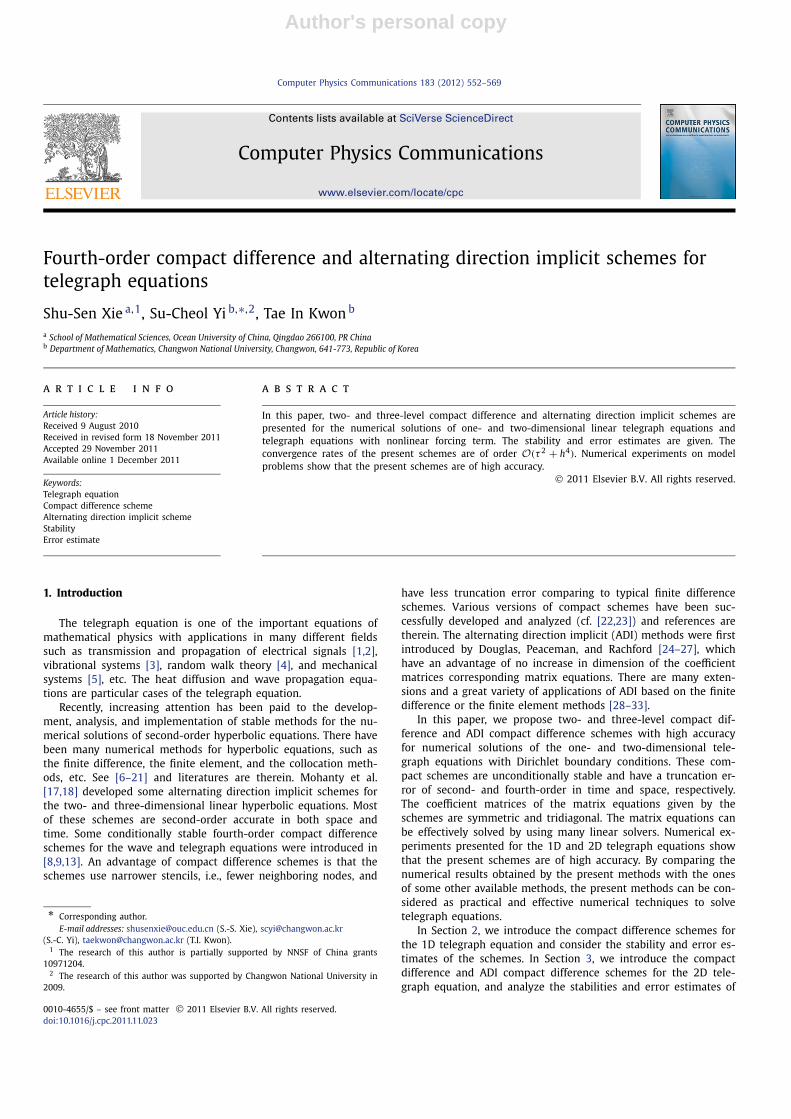
the two-level ADI compact scheme. The errors at times T = 1 and2 are given in Table 10, and this table shows that the convergencerate of the ADI compact scheme is of order O(τ 2 + h4). The con-tour lines of the numerical and exact solutions at t = 2 are drawnin Fig. 5, which shows good agreement between the numerical andexact solutions.

4.2.3. Example 6The exact solution, taken from [32], is given by

u = 1

ωsin(ω(x2 + y2 − 2ac0t

)),

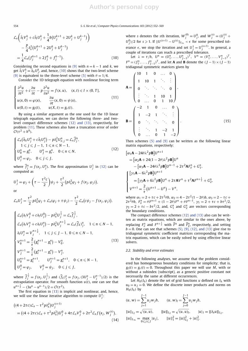
(x, y) ∈ [−1,1] × [−1,1], t × [0, T ],where ω is the angular frequency. The numerical experiments areconducted by taking c = b = 0, p = q = 1, ω = 4π , and a = c0 = 1.Table 11 displays the errors and convergence rates generated bythe two- and three-level ADI compact schemes at time T = 1. Onecan see that the convergence rates of the schemes are of orderO(τ 2 + h4). The numerical and exact solutions, and the contourlines of those solutions generated by 2L-ADI are shown in Fig. 6.One can see that the numerical and exact solutions are in goodagreement.

4.2.4. Example 7In this example, we consider the hyperbolic equation with non-

linear source term

∂2u

∂t2− ∂2u

∂x2− ∂2u

∂ y2+ sin u = 0.

The exact solution, taken from [34], is given by u = 4 ×arctan(exp(x + y − t)). The numerical experiments are conductedby taking Q = [−5,5] × [−5,5]. Table 12 displays the errors andconvergence rates generated by the two- and three-level ADI com-



Fig. 5. Contours of numerical (left) and exact (right) solutions at T = 2 with h = 0.05, τ = 0.0125, p = q = 1, b = 25, and c = 20.

Fig. 6. Profiles and contours of numerical (left) and exact (right) solutions using 2L-ADI scheme at T = 1 with h = 0.01, τ = 0.005.

pact schemes and Table 13 shows the errors generated by 2L-ADIwith different mesh sizes at time T = 4. One can see that theconvergence rate of the two-level scheme is of order O(τ 2 + h4),which is slightly higher than the three-level scheme. The profilesof numerical solutions and errors at T = 4 and 8 are shown inFig. 7.

5. Conclusion and discussion

We proposed the two- and three-level compact difference andADI compact difference schemes with high accuracy for the 1D and2D telegraph equations with Dirichlet boundary conditions. Thetwo-level schemes are unconditionally stable and the three-level



Fig. 7. Profiles of numerical solutions (left) and errors (right) using 2L-ADI scheme at T = 4 (top) and T = 8 (bottom) with h = 0.2, τ = 0.01.

Table 11Errors and convergence order of Example 6 at T = 1.


2L-ADI 1/50 1/50 0.0218 0.03831/100 1/200 0.0013 4.0677 0.0021 4.18891/200 1/800 8.0273E−5 4.0175 1.2672E−4 4.05071/400 1/3200 5.0106E−6 4.0019 7.9248E−6 3.9991

3L-ADI(θ = 1/4)

1/50 1/50 0.0211 0.03991/100 1/200 0.0013 4.0207 0.0025 3.99641/200 1/800 8.3459E−5 3.9613 1.6296E−4 3.93931/400 1/3200 5.5022E−6 3.9230 1.0921E−5 3.8993

3L-ADI(θ = 1/3)

1/50 1/50 0.0325 0.05921/100 1/200 0.0019 4.0964 0.0036 4.03951/200 1/800 1.2202E−4 3.9608 2.3051E−4 3.96511/400 1/3200 7.8955E−6 3.9499 1.5143E−5 3.9281

Table 12Errors and convergence order of Example 7 at T = 4.


2L-ADI 1 4/10 0.6787 0.24851/2 1/10 0.0346 4.2939 0.0153 4.02161/4 1/40 0.0019 4.1867 8.3276E−4 4.19951/8 1/160 1.1803E−4 4.0088 5.1531E−5 4.01441/16 1/640 7.3411E−6 4.0070 3.2145E−6 4.0028

3L-ADI(θ = 1/4)

1 4/10 0.8311 0.29851/2 1/10 0.0608 3.7729 0.0307 3.28141/4 1/40 0.0056 3.4406 0.0030 3.35521/8 1/160 5.9564E−4 3.2329 3.3704E−4 3.15401/16 1/640 6.9255E−5 3.1045 4.7355E−5 2.8313

3L-ADI(θ = 1/2)

1 4/10 1.3183 0.48441/2 1/10 0.0952 3.7916 0.0411 3.55901/4 1/40 0.0074 3.6854 0.0034 3.59551/8 1/160 6.8916E−4 3.4246 3.5812E−4 3.24701/16 1/640 7.4105E−5 3.2172 4.8619E−5 2.8809

Table 13Errors of Example 7 generated by 2L-ADI at T = 4 with different mesh sizes.

h τ ‖e‖L2 ‖e‖L∞

1 1/10 0.4427 0.17411 1/20 0.4201 0.17011/4 1/20 0.0104 0.00411/8 1/20 0.0076 0.00301/8 1/80 8.5216E−4 3.9241E−41/8 1/200 5.7112E−4 3.3248E−41/16 1/200 1.1826E−4 5.7214E−5

compact difference and ADI compact difference schemes are un-conditionally stable for parameters θ in the range of [1/4,1/2].The proposed schemes are second- and fourth-order accurate intime and space, respectively. For the telegraph equations with Neu-mann boundary conditions, the error estimate of order O(τ 2 + h4)

can be obtained by using proper boundary discretization methods(cf. [22,23]). Numerical experiments on test examples show thatour proposed schemes are of high accuracy, and support the the-oretical results. Based on the analyses and numerical experiments,we may say that the proposed schemes are practical and effectivenumerical techniques for solving the 1D and 2D telegraph equa-tions.

Acknowledgements

The authors wish to express their sincere gratitude to the ref-erees for their valuable comments and suggestions on this paper.

References

[1] E.A. Gonzalez-Velasco, Fourier Analysis and Boundary Value Problems, Aca-demic Press, New York, 1995.

[2] P.M. Jordan, A. Puri, Digital signal propagation in dispersive media, J. Appl.Phys. 85 (3) (1999) 1273–1282.

[3] W.E. Boyce, R.C. DiPrima, Differential Equations Elementary and BoundaryValue Problems, Wiley, New York, 1977.



[4] J. Banasiak, J.R. Mika, Singularly perturbed telegraph equations with applica-tions in the random walk theory, J. Appl. Math. Stoch. Anal. 11 (1) (1998) 9–28.

[5] A.N. Tikhonov, A.A. Samarskii, Equations of Mathematical Physics, Dover, NewYork, 1990.

[6] P. Almenar, L. Jódar, J.A. Martin, Mixed problems for the time-dependent tele-graph equation: Continuous numerical solutions with a priori error bounds,Math. Comput. Modelling 25 (11) (1997) 31–44.

[7] R. Aloy, M.C. Casabán, L.A. Caudillo-Mata, L. Jódar, Computing the variable co-efficient telegraph equation using a discrete eigenfunction method, Comput.Math. Appl. 54 (2007) 448–458.

[8] M. Ciment, S.H. Leventhal, Higher order compact implicit schemes for the waveequation, Math. Comp. 29 (1975) 985–994.

[9] M. Ciment, S.H. Leventhal, A note on the operator compact implicit method forthe wave equation, Math. Comp. 32 (1978) 143–147.

[10] G. Dahlquist, On accuracy and unconditional stability of linear multi-stepmethods for second order differential equations, BIT 18 (1978) 133–136.

[11] M. Dehghan, A. Mohebbi, High order implicit collocation method for the solu-tion of two-dimensional linear hyperbolic equation, Numer. Methods PDEs 25(2009) 232–243.

[12] M. Dehghan, A. Shokri, A numerical method for solving the hyperbolic tele-graph equation, Numer. Methods PDEs 24 (2008) 1080–1093.

[13] H. Ding, Y. Zhang, A new fourth-order compact finite difference scheme for thetwo-dimensional second-order hyperbolic equation, J. Comp. Appl. Math. 230(2009) 626–632.

[14] M.S. El-Azab, M. El-Gamel, A numerical algorithm for the solution of telegraphequations, Appl. Math. Comput. 190 (2007) 757–764.

[15] L. Jódar, D. Goberna, Analytic-numerical solution with a priori error bounds forcoupled time-dependent telegraph equations: Mixed problems, Math Comput.Modelling 30 (1999) 39–53.

[16] R.K. Mohanty, An unconditionally stable difference scheme for the one-space-dimensional linear hyperbolic equation, Appl. Math. Lett. 17 (2004) 101–105.

[17] R.K. Mohanty, M.K. Jain, An unconditionally stable alternating direction implicitscheme for the two space dimensional linear hyperbolic equation, Numer.Methods PDEs 17 (2001) 684–688.

[18] R.K. Mohanty, M.K. Jain, U. Arora, An unconditionally stable ADI method forthe linear hyperbolic equation in three space dimensions, Int. J. Comput.Math. 79 (2002) 133–142.

[19] R.K. Mohanty, M.K. Jain, K. George, High order difference schemes for the sys-tem of two space second order nonlinear hyperbolic equations with variablecoefficients, J. Comp. Appl. Math. 70 (1996) 231–243.

[20] R.K. Mohanty, M.K. Jain, K. George, On the use of high order difference meth-ods for the system of one space second order non-linear hyperbolic equationswith variable coefficients, J. Comp. Appl. Math. 72 (1996) 421–431.

[21] E.H. Twizell, An explicit difference method for the wave equation withextended stability range, BIT 19 (1979) 378–383.

[22] J. Zhao, W. Dai, T. Niu, Fourth-order compact schemes of a heat conductionproblem with Neumann boundary conditions, Numer. Methods PDEs 23 (2007)949–959.

[23] J. Zhao, W. Dai, S. Zhang, Fourth-order compact schemes for solving mul-tidimensional heat problems with Neumann boundary conditions, Numer.Methods PDEs 24 (2008) 165–178.

[24] J.Jr. Douglas, On the numerical integration of ∂2u∂x2 + ∂2u

∂ y2 = ∂u∂t by implicit

methods, J. Soc. Indust. Appl. Math. 3 (1955) 42–65.[25] J.Jr. Douglas, D. Peaceman, Numerical solution of two-dimensional heat flow

problems, AIChE Journal 1 (1955) 505–512.[26] J.Jr. Douglas, H. Rachford, On the numerical solution of heat conduction prob-

lems in two and three space variables, Trans. Amer. Math. Soc. 82 (1960)421–439.

[27] D. Peaceman, H. Rachford, The numerical solution of parabolic and ellipticequations, J. Soc. Indust. Appl. Math. 3 (1955) 28–41.

[28] C. Clavero, J.L. Gracia, J.C. Jorge, A uniformly convergent alternating directionHODIE finite difference scheme for 2D time-dependent convection–diffusionproblems, IMA J. Numer. Anal. 26 (2006) 155–172.

[29] C. Clavero, J.C. Jorge, F. Lisbona, G.I. Shishkin, A fractional step method on aspecial mesh for the resolution of multidimensional evolutionary convection–diffusion problems, Appl. Numer. Math. 27 (1998) 211–231.

[30] C. Clavero, J.C. Jorge, F. Lisbona, G.I. Shishkin, An alternating direction schemeon a nonuniform mesh for reaction–diffusion parabolic problems, IMA J.Numer. Anal. 20 (2000) 263–280.

[31] S. Kim, H. Lim, High-order schemes for acoustic waveform simulation, Appl.Numer. Math. 57 (2007) 402–414.

[32] H. Lim, S. Kim, J.Jr. Douglas, Numerical method for viscous and non-viscouswave equations, Appl. Numer. Math. 57 (2) (2007) 194–212.

[33] N.N. Yanenko, The Method of Fractional Steps, Springer-Verlag, New York, 1971.[34] K. Djidjeli, W.G. Price, E.H. Twizell, Numerical solutions of a damped sine-

Gordon equation in two space variables, J. Engrg. Math. 29 (1995) 347–369.

Offprint CPC2012

Documents

Transcript of Offprint CPC2012