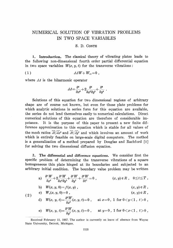
NUMERICAL SOLUTION OF VIBRATION PROBLEMS

IN TWO SPACE VARIABLES

S. D. CONTE

l Introduction* The classical theory of vibrating plates leads tothe following non-dimensional fourth order partial differential equationin two space variables W(x, y, t) for the transverse vibrations:

(1) ΔΔW+Wtt = 0 ,

where ΔΔ is the biharmonic operator

dx2dy2 dtf

Solutions of this equation for two dimensional regions of arbitraryshape are of course not known, but even for those plate problems forwhich analytic solutions in series form for this equation are available,the series do not lend themselves easily to numerical calculations. Directnumerical solutions of this equation are therefore of considerable im-potance. It is the purpose of this paper to present a new finite dif-ference approximation to this equation which is stable for all values ofthe mesh ratios Δt/Δx2 and Δt\Δy2 and which involves an amount of workwhich is entirely feasible on large-scale digital computers. The methodis a generalization of a method prepared by Douglas and Rachford [1]for solving the two dimensional diffusion equation.

2. The differential and difference equations* We consider first thespecific problem of determining the transverse vibrations of a squarehomogeneous thin plate hinged at its boundaries and subjected to anarbitrary initial condition. The boundary value problem may be written

*W+2*WL+*W+»W = Ot (x,y)eR, 0<t<T,dxi dtfdy2 dy* ΘP

b) W(x,y,0)=f(x,y), (x,y)eR,

c) Wt(x,y,0) = 0, (x,y)eR,

d) W(x, y, t)=^-(x, y, ί)=0 , at x=0, 1 for 0<y<l , t>0 ,

e) Wix, y, t)=^~(x, y, ί)=0 , at y=0 , 1 for 0 θ < l , ί>0 ,dy*

Received February 11, 1957. The author is currently on leave of absence from WayneState University, Detroit, Michigan.

1535

1536 S. D. CONTE

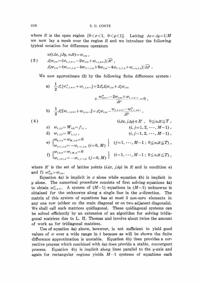
where R is the open region \0<x<l, 0<y<Y\. Letting Δx=Δy=^l/Mwe now lay a mesh over the region R and we introduce the followingtypical notation for difference operators

w{iΔx,jΔy, nΔt) = wίjn

We now approximate (2) by the following finite difference system :

a) — Δi[wZJ,n+ι+wίJ>n-1]+2Δldlwijn+ΔtJwijn

1

n - . 1 j A y W i j n ,

£ Δt"

( 4 ) (iΔx, jΔy) e # ' , O^nAt^ T ,

c) Wij,o=Wυo=fυ , (i, j=l,2, — , Λf—1) ,

d) w M > 1 = TFIJ>0 , («,ί = l ,2 , . . . , 3 f - l ) ,

,. n Λ / f, (ί = l , . . . , Λ ί - l

(^.=^..=0 , ( H - , I - l ; 0 ^Ki+i,m=-^j-i,« O = 0, M) )

where β r is the set of lattice points {iΔx, jΔy) in R and in condition e)and f) wfjn^wijn.

Equation 4a) is implicit in x alone while equation 4b) is implicit iny alone. The numerical procedure consists of first solving equations 4a)to obtain wfj>n+1. A system of (M— 1) equations in (Λf— 1) unknowns isobtained for the unknowns along a single line in the a -direction. Thematrix of this system of equations has at most 5 non-zero elements inany one row (either on the main diagonal or on two adjacent diagonals).We shall call such matrices quidiagonal. These quidiagonal systems canbe solved efficiently by an extension of an algorithm for solving tridia-gonal matrices due to L. H. Thomas and involve about twice the amountof work as for tridiagonal matrices.

Use of equation 4a) above, however, is not sufficient to yield goodvalues of w over a wide range in t because as will be shown the finitedifference approximation is unstable. Equation 4b) then provides a cor-rective process which combined with 4a) does provide a stable, convergentprocess. Equation 4b) is implicit along lines parallel to the y-axis andagain for rectangular regions yields Λf—1 systems of equations each

NUMERICAL SOLUTION OF VIBRATION PROBLEMS 1537

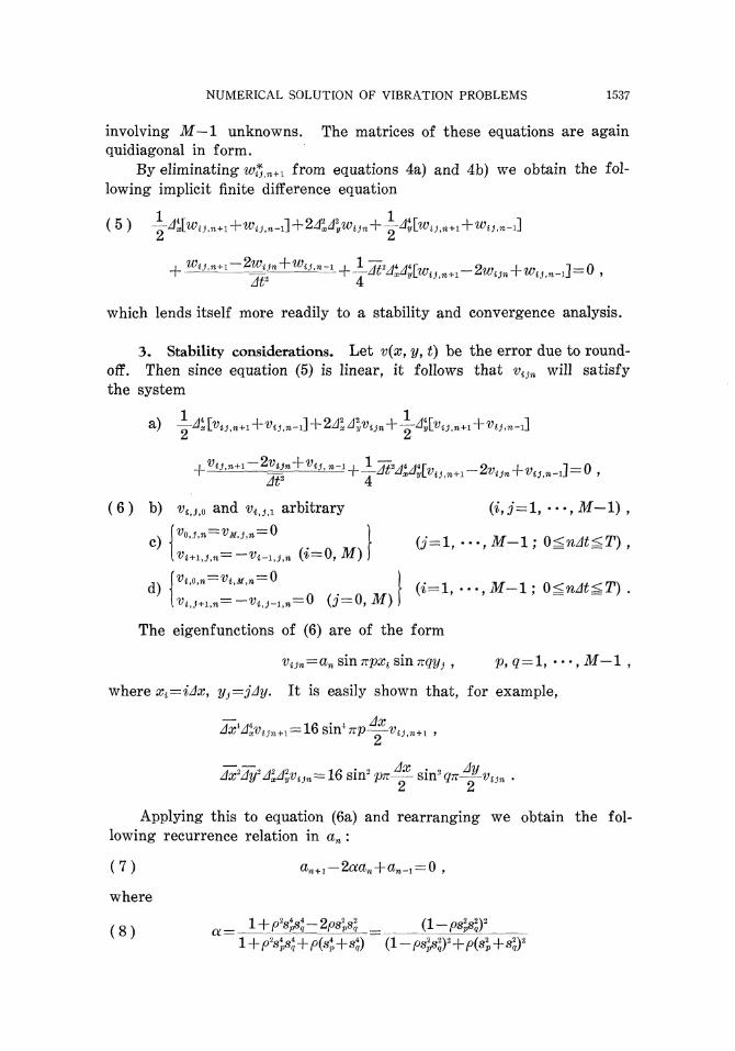
involving M— 1 unknowns. The matrices of these equations are againquidiagonal in form.

By eliminating wfjyn+ι from equations 4a) and 4b) we obtain the fol-lowing implicit finite difference equation

( 5 ) —dAJiwtjtn+1+wiJtn-1]+2/Pad\,wiJn +Δ Δ

Γ 2

which lends itself more readily to a stability and convergence analysis.

3* Stability considerations* Let v(x, y, t) be the error due to round-off. Then since equation (5) is linear, it follows that vijn will satisfythe system

a) - 4 K J ) M + 1 + ^ j ) W - 1 ] + 2 4 J > ί i n + - φ i J i n + 1 4 - v i j , n - 1 ]Δ Δ

I = = /Γ vJ. j j,Zίt' 4

( 6 ) b) v<Jι0 and v 4 J f l arbitrary (i,^"=l, , M—1) ,

c)ij,n=--v<-1j> n (*=0, M)

Ί x f / y ί 0

d) iJ+l,n=--'W«J-l,n=O 0 = 0 , Λf)

The eigenfunctions of (6) are of the form

vίjn=cin sin 7rpa?t sin πqy3 , p, g = l , , M— 1 ,

where xi — iΔx, y^jΔy. It is easily shown that, for example,

3n=16 sin3

Applying this to equation (6a) and rearranging we obtain the fol-lowing recurrence relation in an :

where

( 8 ) a- 1+P24sQ~2psls2

q = (l-ps2

ps2

q)2

1538 S. D. CONTE

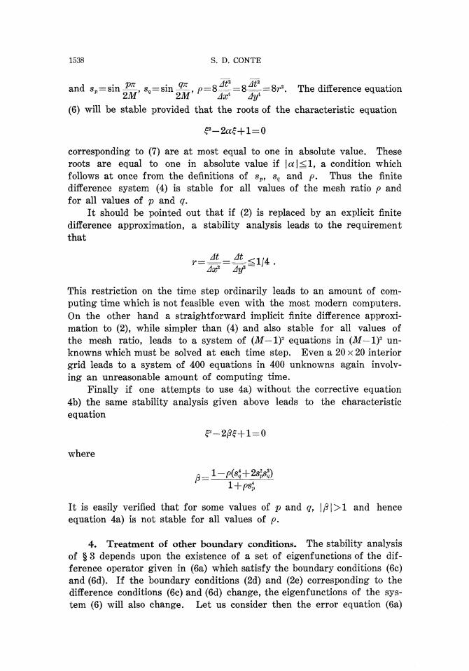
and β,=sin ^- sg=sin M-, p=δiζ=δi£=8r2. The difference equation

(6) will be stable provided that the roots of the characteristic equation

corresponding to (7) are at most equal to one in absolute value. Theseroots are equal to one in absolute value if | α | ^ l , a condition whichfollows at once from the definitions of sp, sq and p. Thus the finitedifference system (4) is stable for all values of the mesh ratio p andfor all values of p and q.

It should be pointed out that if (2) is replaced by an explicit finitedifference approximation, a stability analysis leads to the requirementthat

This restriction on the time step ordinarily leads to an amount of com-puting time which is not feasible even with the most modern computers.On the other hand a straightforward implicit finite difference approxi-mation to (2), while simpler than (4) and also stable for all values ofthe mesh ratio, leads to a system of (ikf—I)2 equations in (M—lf un-knowns which must be solved at each time step. Even a 20 x 20 interiorgrid leads to a system of 400 equations in 400 unknowns again involv-ing an unreasonable amount of computing time.

Finally if one attempts to use 4a) without the corrective equation4b) the same stability analysis given above leads to the characteristicequation

where

It is easily verified that for some values of p and q, \β\>l and henceequation 4a) is not stable for all values of p.

4- Treatment of other boundary conditions* The stability analysisof § 3 depends upon the existence of a set of eigenfunctions of the dif-ference operator given in (6a) which satisfy the boundary conditions (6c)and (6d). If the boundary conditions (2d) and (2e) corresponding to thedifference conditions (6c) and (6d) change, the eigenf unctions of the sys-tem (6) will also change. Let us consider then the error equation (6a)

NUMERICAL SOLUTION OF VIBRATION PROBLEMS 1539

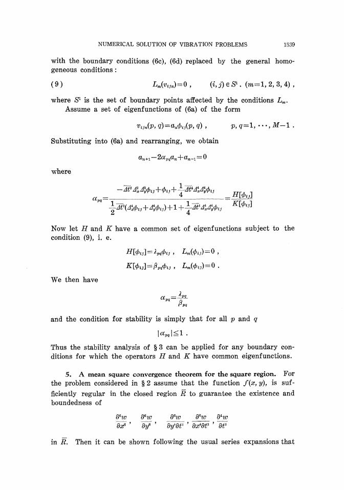
with the boundary conditions (6c), (6d) replaced by the general homo-geneous conditions :

(9) Lm(vijn)=0 , («, j) e S 1 . (m=l, 2, 3, 4) ,

where S1 is the set of boundary points affected by the conditions Lm.Assume a set of eigenfunctions of (6a) of the form

vi3n{v, q)=a>nΦιAPf Q) > p, g = l , , Λf-1 .

Substituting into (6a) and rearranging, we obtain

an+1-2apqan+an-1=0

where

Now let H and if have a common set of eigenfunctions subject to thecondition (9), i. e.

We then have

«„=!»•

and the condition for stability is simply that for all p and q

Thus the stability analysis of § 3 can be applied for any boundary con-ditions for which the operators H and K have common eigenfunctions.

5 A mean square convergence theorem for the square region. For

the problem considered in § 2 assume that the function f(x, y), is suf-

ficiently regular in the closed region R to guarantee the existence and

boundedness of

dQw dSΌ dQw dQw dHυ

in R. Then it can be shown following the usual series expansions that

1540 S. D. CONTE

(10)

I

and moreover that

(11) Jt^Al[wίJtn+1-

Hence the difference operator (5) approximates the differential equation

(2) to terms which are 0(Ax2+At2). In the notation of [2] the elementary

truncation error hίjn is

(12) h^

and by Theorem 1 of [2] we have

(13) \\Wijn-wijn

uniformly in n, where

(14) 1 J F f J n _ w < J n | = ^ ^ { J ί 1 Wijn -

It thus follows that if the boundary value problem (2) is sufficiently

well defined in the sense that the derivatives mentioned above exist

boundedly in the closed region R, then the solution of (4) converges in

the mean to the solution of (2) with errors given by (13) as Δx and At

tend to zero.The convergence proof given above holds for a rectangular region

only. In practice one is usually interested in point-wise convergencerather than convergence in the mean square sense. Section 6 establishespoint-wise convergence of the solution of the difference system to thesolution of the differental system.

6. Point-wise convergence* A solution of the boundary value prob-lem (2) can be given in series form

oo eβ

(15) W(x, i/,ί) = Σ Σ Apq sin pπx sin qπy cos (p2+q2)π2t .

The initial condition (2b) will be satisfied provided that Apq are taken tobe the Fourier coefficients of f(x, y), i.e.

(16) Am=4: \ \ f(x, y) sin pπx sin qπy dxdy .Jo Jo

NUMERICAL SOLUTION OF VIBRATION PROBLEMS 1541

The conditions on f(x, y) are assumed to be such that the series(15) converges and is the unique solution of the boundary value problem(2). A solution w(x, y, t) of the finite difference system consisting of(4a, b, e, f) can be obtained by separation of variables as follows :

(17) w(x, κ,ί) = Σ Σ Bm sin pπx sin qπy cos ^ - arc cos M ΐ ^ ,p-i «-i r λ2(p, q)

where

and Bpq are arbitrary constants. The series (17) satisfies the finite dif-ference system (4) except for the initial condition 4c).

We will now show that it is possible to choose the coefficients Bpq

so that the solution w(x, yf t) of the difference system will converge tothe solution W{x,y,t) of the differential system as Λf-*oo. We firstdefine an integer k(M) such that k(M)<M1>5 and limk(M)=oo. We

M-*oo

then choose the Bpq so that Bpq = 0 for p>k(M), q>k(M) and the re-maining Bpq so that for any e>0 there exists an M^ε) such that forM>Mlf

(18) \BPQ-Apq\<εM-*15 uniformly for p, g = l , , k{M) .

One way of satisfying (18) for instance is to choose Bm—Apa for p, g=1, •• , k(M). An exact solution of the difference equation then is

(19) wM(x, y,t)~ Σ Σ Bpq sin pπx sin qπy cos arc cos —- .

This solution satisfies the initial condition

k k

(20) wM(x, y, 0) = Σ Σ ^PQ sin p πE sin g r?/

and of course does not satisfy the exact initial condition w(x, y, 0) =/(#, ?/). However, it will satisfy this initial condition in the limit asM - > o o .

LEMMA 1. For any p>0, Ogz^—ikf-*'5, 0^z2^—M~φ, there

exists an M2(p) such that for M>M2 and for any ε>0

(21) 4r(zl+zϊ)-arc cos^ <r ε

1542

where

S. D. CONTE

λι=(l—p sin2 z1 sin2 z2f ,

λ2=(1—p sin2 #! sin2 z2)2+p(sin2 zL+sin2 z.zf .

Proof. We first choose Mz{p) such that Λf>ikf3 and for all admis-sible zlf z2

(22)

Let

F(zlf z 2 ) -

It is obvious that F(0,0) — 0 and it can be shown by direct calculationthat the partial derivatives of F(zlf z2) up to and including those of order3 all vanish at ^ = 0 , z2=0. Thus in the Taylor series expansion ofF(zl9 zz) the remainder term is

where the coefficients ^(^,^2), i=( l , « ,5), are related to the fourth

derivatives of Ffe, z2) and 0<^<—ikf"4/5, 0^^2<—M"4 / 5. Using theΔ Δ

inequality (22) it is possible to show that the au are bounded functionsof p. Thus using the extreme limits of zι, z2 we have

\F(zlf z.m

and hence it follows that there exists an M2(p) such that for M>M2,

as the lemma asserts.

Now multiplying (21) by and putting z1—^-, zi=-^- we haver 2M 2M

and therefore

(23)

UP, Q)

cos M!L arc cos λ^p> g ) - c o s π2

^M'

NUMERICAL SOLUTION OF VIBRATION PROBLEMS 1543

THEOREM 1 (THE CONVERGENCE THEOREM). Under the assumptions

a) t>0 , 0 < # < l , 0 < 2 / < l ; p>0 p,t,x,y fixed

b) I Apq\<^P , P constant, for all p, q=l, 2, , oo

c) k(M)<M115 , Urn k(M)= oo

d) \Bpq~A

we have

lim wM(x, y, £)= W(x, y, t)

or

Σ Σ B(M) sin pττα; sin qπy cos ^ i arc cos ΛΛPr q)lim Σ Σ Bpz(M) sin pπx sin qπy cos arc cos :

M—>o° ϋ = l (7 = 1 Ύ*

oo oo

= Σ Σ Apq sin pπx sin g7r?/ cos (p2+q2)π2t .

Proo/.

wM{x, y, t)— W(x, y,t)—^Σ, Σ {Bp(l—Apq) sin pτr# sin qπy cos (p2+q2)π2t

+ Σ Σ (̂ Bpg—Apq) sin pπα; sin g7rJ cos arc cos ——cos (p2+q2)π2tp=iq=i L r l2 J

+ Σ Σ Apq sin p7rίc sin qπy\ cos arc cos ——cos (p2+q2)π2t1 1 L r λ« J

+ Σ Σ .̂pg sin p7rίc sin qπy cosfc + l fc + 1

By conditions c) and d) above and Lemma 1,

M M

By condition b) and c) and Lemma 1,

and because the series for w(x, y, t) converges there exists an Λf4 suchthat for M>M,

1544 S. D. CONTE

Thus for M>max(M 1 , Af2, Λf4),

\WM(X, V, t)-W(x, y, t)\^

This establishes the convergence theorem.

REFERENCES

1. J. Douglas and H. Rachford, On the numerical solutions of heat conduction problemsin two and three space variables, Trans. Amer. Math. Soc. (1956), 421-439.2. J. Douglas, On the relation between stability and convergence in the numerical solutionof linear parabolic and hyperbolic differential equations, J. Soc. Ind. Appl. Math., 4(1956), 20-38.

T H E RAMO-WOOLDRIDGE CORPORATION