Numerical modeling and phase prediction in deep overpressured basinal settings of the Central Graben,

North Sea

vorgelegt von Dipl.-Geologe

Volkmar Neumann aus Berlin

Von der Fakultät VI der Technischen Universität Berlin

zur Erlangung des akademischen Grades

Doktor der Naturwissenschaften - Dr. rer. nat. -

genehmigte Dissertation

Promotionsausschuss:

Vorsitzender: Prof. Dr. G. Franz Berichter: Prof. Dr. B. Horsfield Berichter: Prof. Dr. W. Dominik

Tag der wissenschaftlichen Aussprache: 11. Dezember 2006

Berlin 2007

D 83

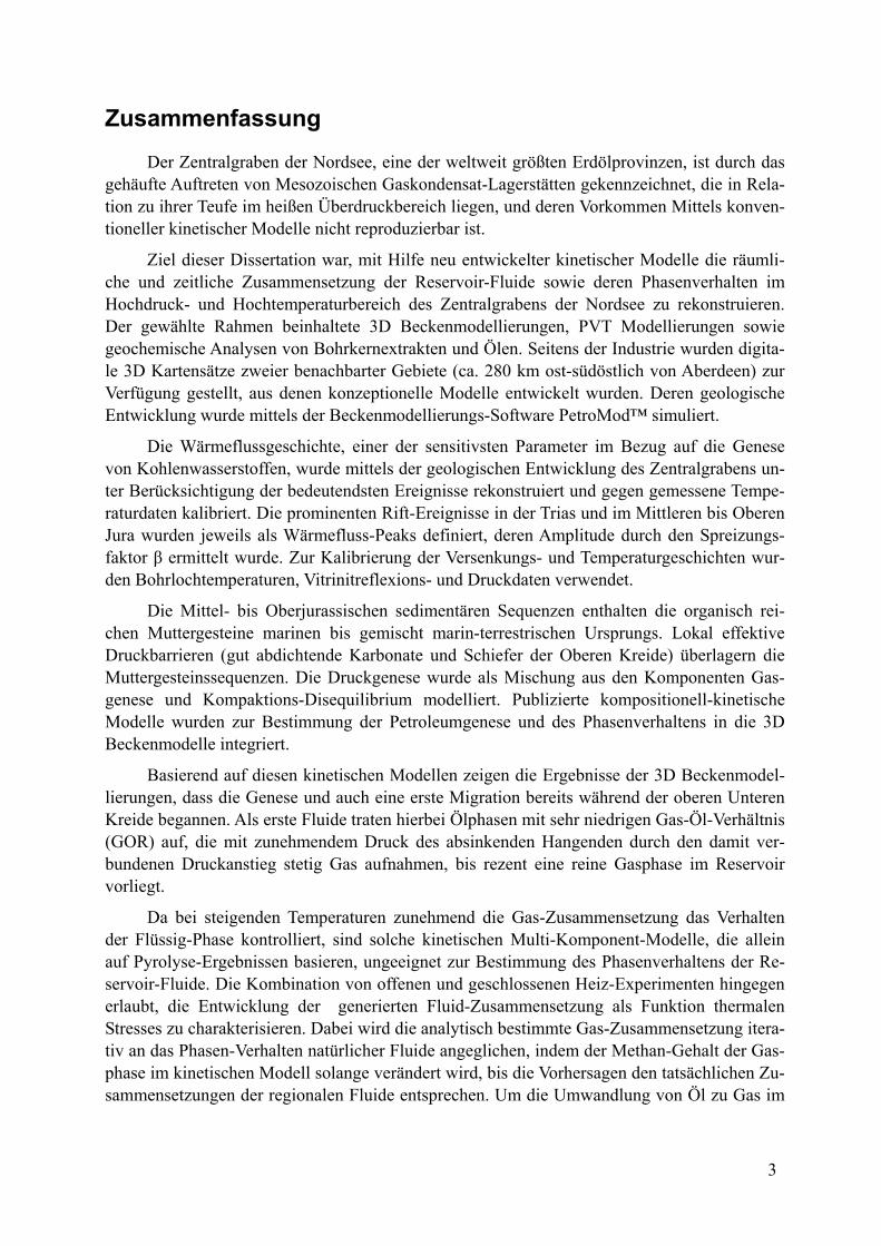
Zusammenfassung

Der Zentralgraben der Nordsee, eine der weltweit größten Erdölprovinzen, ist durch das gehäufte Auftreten von Mesozoischen Gaskondensat-Lagerstätten gekennzeichnet, die in Rela-tion zu ihrer Teufe im heißen Überdruckbereich liegen, und deren Vorkommen Mittels konven-tioneller kinetischer Modelle nicht reproduzierbar ist.

Ziel dieser Dissertation war, mit Hilfe neu entwickelter kinetischer Modelle die räumli-che und zeitliche Zusammensetzung der Reservoir-Fluide sowie deren Phasenverhalten im Hochdruck- und Hochtemperaturbereich des Zentralgrabens der Nordsee zu rekonstruieren. Der gewählte Rahmen beinhaltete 3D Beckenmodellierungen, PVT Modellierungen sowie geochemische Analysen von Bohrkernextrakten und Ölen. Seitens der Industrie wurden digita-le 3D Kartensätze zweier benachbarter Gebiete (ca. 280 km ost-südöstlich von Aberdeen) zur Verfügung gestellt, aus denen konzeptionelle Modelle entwickelt wurden. Deren geologische Entwicklung wurde mittels der Beckenmodellierungs-Software PetroMod™ simuliert.

Die Wärmeflussgeschichte, einer der sensitivsten Parameter im Bezug auf die Genese von Kohlenwasserstoffen, wurde mittels der geologischen Entwicklung des Zentralgrabens un-ter Berücksichtigung der bedeutendsten Ereignisse rekonstruiert und gegen gemessene Tempe-raturdaten kalibriert. Die prominenten Rift-Ereignisse in der Trias und im Mittleren bis Oberen Jura wurden jeweils als Wärmefluss-Peaks definiert, deren Amplitude durch den Spreizungs-faktor β ermittelt wurde. Zur Kalibrierung der Versenkungs- und Temperaturgeschichten wur-den Bohrlochtemperaturen, Vitrinitreflexions- und Druckdaten verwendet.

Die Mittel- bis Oberjurassischen sedimentären Sequenzen enthalten die organisch rei-chen Muttergesteine marinen bis gemischt marin-terrestrischen Ursprungs. Lokal effektive Druckbarrieren (gut abdichtende Karbonate und Schiefer der Oberen Kreide) überlagern die Muttergesteinssequenzen. Die Druckgenese wurde als Mischung aus den Komponenten Gas-genese und Kompaktions-Disequilibrium modelliert. Publizierte kompositionell-kinetische Modelle wurden zur Bestimmung der Petroleumgenese und des Phasenverhaltens in die 3D Beckenmodelle integriert.

Basierend auf diesen kinetischen Modellen zeigen die Ergebnisse der 3D Beckenmodel-lierungen, dass die Genese und auch eine erste Migration bereits während der oberen Unteren Kreide begannen. Als erste Fluide traten hierbei Ölphasen mit sehr niedrigen Gas-Öl-Verhältnis (GOR) auf, die mit zunehmendem Druck des absinkenden Hangenden durch den damit ver-bundenen Druckanstieg stetig Gas aufnahmen, bis rezent eine reine Gasphase im Reservoir vorliegt.

Da bei steigenden Temperaturen zunehmend die Gas-Zusammensetzung das Verhalten der Flüssig-Phase kontrolliert, sind solche kinetischen Multi-Komponent-Modelle, die allein auf Pyrolyse-Ergebnissen basieren, ungeeignet zur Bestimmung des Phasenverhaltens der Re-servoir-Fluide. Die Kombination von offenen und geschlossenen Heiz-Experimenten hingegen erlaubt, die Entwicklung der generierten Fluid-Zusammensetzung als Funktion thermalen Stresses zu charakterisieren. Dabei wird die analytisch bestimmte Gas-Zusammensetzung itera-tiv an das Phasen-Verhalten natürlicher Fluide angeglichen, indem der Methan-Gehalt der Gas-phase im kinetischen Modell solange verändert wird, bis die Vorhersagen den tatsächlichen Zu-sammensetzungen der regionalen Fluide entsprechen. Um die Umwandlung von Öl zu Gas im

3

Model zu definieren, wurde die Stabilität der Flüssig-Phase-Komponenten systematisch im Rahmen publizierter Resultate variiert. Methan wurde hierbei als einziges Produkt der Ölum-wandlung definiert. Derart erstellte kinetische Multi-Komponent-Modelle wurden den ver-schiedenen Muttergesteinssequenzen in den Beckensimulationen zugewiesen.

Die Ergebnisse zeigen einen zeitlichen und ursächlichen Zusammenhang zwischen Druck- und Temperaturentwicklung und Phasenverhalten. Vor allem ist die Entwicklung von Überdruck verantwortlich für die heute vorkommenden untersättigten Reservoir-Fluide. Die Reservoire enthielten während der ersten Füllung ein gasdominiertes, zweiphasiges Fluid, das erst nach Einstellung des Überdrucks den heutigen untersättigten Zustand erreichte.

Durch die Verflechtung von kompositionellen Daten von offenen und geschlossenen Heiz-Experimenten sowie regionalen PVT Daten konnte ein kinetisches Multi-Komponent-Modelle erstellt werden, das die beobachteten Fluid-Zusammensetzungen sowie deren physika-lischen Eigenschaften korrekt reproduzieren konnte. Die Kombination der Ergebnisse der Be-ckenmodellierung, PVT Modellierung und geochemischer Analytik ermöglicht die Identifizie-rung der Hauptprozesse, die im Verlauf der Fluidentwicklung in den Hochdruck- und Hoch-temperaturbereichen der Mesozoischen Reservoire des Zentralgrabens in Raum und Zeit auf-traten.

Abstract

The North Sea, and especially the Central Graben area, is one of the world’s major petro-leum provinces. The occurrence of gas condensates is a typical feature of many Central Graben Mesozoic reservoirs. The reservoirs are here highly overpressured and have elevated tempera-tures. Based on conventional kinetic schemes their occurrence is not explicable.

Goal of this study was to reproduce the chemical composition of these reservoir fluids in space and time, and their phase behavior, using newly developed compositional kinetic models, based in the framework of 3D basin modeling, PVT modeling and geochemical analyses of core extracts and live fluids.

3D digital map sets of two neighboring areas (approx. 280 km eats-southeast of Aber-deen) were supplied by the petroleum industry partners. These maps and additional data were used to develop a conceptual model on which basin modeling (PetroMod™ software) was per-formed. The thermal history of the basins, one of the most sensitive parameter with respect to hydrocarbon genesis, was reproduced using the published geological history of the Central Graben and its most prominent events and calibrated using well data. The Triassic and Middle to Upper Jurassic rifting events, which affected to a large extent the Graben system, were de-fined as thermal spikes; their amplitude was reconstructed using the spreading factor β. Addi-tional calibration data included Vitrinite reflectance data and pressure measurements.

The Middle to Upper Jurassic sedimentary sequences include the organic rich source rocks of marine to mixed marine-terrestrial origin, overlain by tight Cretaceous shales and car-

4

bonates which both act locally as effective pressure seals. The development of overpressure was included into the basin models as a feature of mixed origin, consisting of both gas genera-tion and disequilibrium compaction. Published compositional kinetic models were assigned to the different source rock intervals in the basin models to evaluate hydrocarbon generation and phase behavior. The 3D basin modeling results based on these kinetic models indicate that gen-eration and migration of hydrocarbons started already early during the upper Early Cretaceous. An oil dominated fluid with a low GOR was the first fluid emplacement. With the onset of overpressure due to accelerated burial, the fluid became gas richer. Present day reservoir fluid is a pure gas phase.

With rising temperatures, the composition of the gas phase dominantly controls the be-havior of the fluid phase. Therefore, multi compound kinetic models purely based on results achieved from pyrolysis experiments are not suitable for any exact prediction on phase behav-ior of the reservoir fluids.

The combination of open and closed system heating experiments allows characterizing the evolution of the fluid’s composition as a function of thermal stress. Gas compositions de-termined analytically are tuned to natural fluid phase behavior and the ensuing “corrected” gas compositions used for the definition of multi-compound kinetic models. To define the conver-sion of oil to gas in the model, the stability of the liquid phase compounds was systematically varied within the framework of published results, with methane being defined as the only product of oil conversion. Such defined multi-compound kinetic models were assigned in the basin models to the different source rock sequences.

Results indicate a connection between pressure- and temperature development and phase behavior. Especially the generation of severe overpressure is responsible for the occurrence of the present day encountered undersaturated reservoir fluids. At first charge, the reservoirs con-tained a vapor dominated two-phase fluid, which became undersaturated after the onset of se-vere overpressure.

The integration of compositional data from open and closed heating experiments together with regional PVT data allowed defining a compositional kinetic model which enables to re-produce the observed fluid composition and physical properties through time. The combined results from basin modeling, PVT modeling and geochemical analysis allowed identifying the main processes, which took place during the evolution of the investigated Mesozoic HPHT reservoirs through time and space.

Schlagwörter:

Zentralgraben Nordsee, 3D Beckenmodellierung, Kinetische Modelle, Druckmodellierung

Keywords:

North Sea Central Graben, 3D Basin Modeling, Compositional Kinetics, Pressure Modeling

5

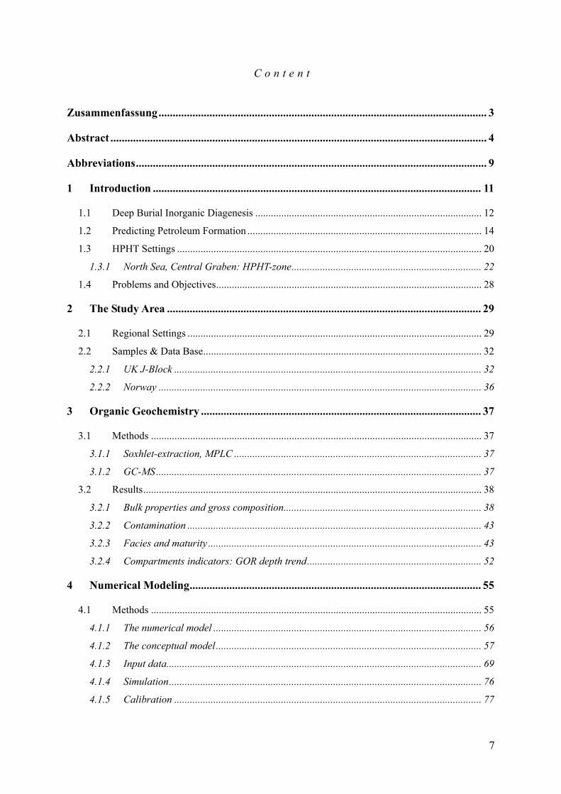
C o n t e n t

Zusammenfassung.................................................................................................................... 3

Abstract ..................................................................................................................................... 4

Abbreviations............................................................................................................................ 9

1 .................................................................................................................... 11 Introduction

1.1 ....................................................................................... 12 Deep Burial Inorganic Diagenesis

1.2 .......................................................................................... 14 Predicting Petroleum Formation

1.3 ..................................................................................................................... 20 HPHT Settings

1.3.1 ......................................................................... 22 North Sea, Central Graben: HPHT-zone

1.4 ...................................................................................................... 28 Problems and Objectives

2 ............................................................................................................... 29 The Study Area

2.1 ................................................................................................................. 29 Regional Settings

2.2 ........................................................................................................... 32 Samples & Data Base

2.2.1 ...................................................................................................................... 32 UK J-Block

2.2.2 ............................................................................................................................ 36 Norway

3 ................................................................................................... 37 Organic Geochemistry

3.1 ............................................................................................................................... 37 Methods

3.1.1 ............................................................................................... 37 Soxhlet-extraction, MPLC

3.1.2 ............................................................................................................................. 37 GC-MS

3.2 .................................................................................................................................. 38 Results

3.2.1 ............................................................................ 38 Bulk properties and gross composition

3.2.2 ................................................................................................................. 43 Contamination

3.2.3 ......................................................................................................... 43 Facies and maturity

3.2.4 ................................................................... 52 Compartments indicators: GOR depth trend

4 ....................................................................................................... 55 Numerical Modeling

4.1 ............................................................................................................................... 55 Methods

4.1.1 ....................................................................................................... 56 The numerical model

4.1.2 ...................................................................................................... 57 The conceptual model

4.1.3 ......................................................................................................................... 69 Input data

4.1.4 ........................................................................................................................ 76 Simulation

4.1.5 ...................................................................................................................... 77 Calibration

7

4.1.6 ........................................................................................................... 80 Sensitivity analysis

4.1.7 ................................................................... 80 Kinetic modeling of hydrocarbon formation

4.2 .................................................................................................................................. 82 Results

4.2.1 ............................................................................................................ 82 Pressure histories

4.2.2 ............................................................................................................. 99 Thermal histories

4.2.3 ........................................................................................ 108 Maturation & filling histories

5 ...................................................................................................................... 137 Discussion

6 ................................................................................................................... 142 Conclusions

References ............................................................................................................................. 145

Acknowledgements............................................................................................................... 161

Index of Figures .................................................................................................................... 162

Index of Tables...................................................................................................................... 166

Appendix I: Basin Modeling Data Input............................................................................ 167

Appendix II: Compositional Kinetic Models ..................................................................... 169

Appendix III: Photo Plate.................................................................................................... 173

Appendix IV: Geochemical Data......................................................................................... 174

Appendix V: Biomarkers ..................................................................................................... 186

8

Abbreviations

A Activation Energy API Gravity °API = (141.5 / specific gravity at 60°F) – 131.5 β Beta factor for crustal stretching modeling BHT Bottom Hole Temperature CPI Carbon Preference Index °C °Celsius DST Drill Stem Test E East E Frequency Factor a

EOS Equation of State GC Gas Chromatography GC-MS Gas Chromatography – Mass Spectrometry GOR Gas-Oil-Ratio HC Hydrocarbons HI Hydrogen Index (mg HC/g TOC) HPHT High Pressure – High Temperature K Kelvin Ma Million Years mD milli-Darcy MPa Mega Pascal MPI Methylphenanthrene Index MPLC Medium Pressure Liquid Chromatography MSSV Micro-Scaled Sealed Vessel N North

Pressure, reduced Pressure, Saturation Pressure P, Pr, Psat

Pr/Ph Pristane/Phytane Ratio pT Pressure-Temperature PVT Pressure, Volume, Temperature RFT Repeat Formation Test S South T, T , T Temperature, reduced Temperature, critical temperature r c

TOC Total Organic Carbon TVDSS True Vertical Depth Sub Sea W West Z Compressibility Factor (Gas)

9

1 Introduction

The Central Graben is one of the world’s major oil provinces, which has followed a typi-cal exploitation path for a hydrocarbon producing area, with large conventional fields being developed first and thereafter smaller fields, utilizing the existing infrastructure. It contains oil, gas and gas condensates in reservoirs of Devonian to Early Eocene age. Of special current in-terest is the development of technically challenging fields in hot and severely overpressured settings (HPHT). The reservoirs show general similarities in that they represent structural traps, varying from faulted anticlines like for example in the British Elgin Field (North Sea) to horst-shaped, tilted fault blocks as being encountered in the Franklin Field. These reservoirs are characterized by the occurrence of extensive secondary porosity resulting from feldspar grain and carbonate cement dissolution. This secondary porosity is best preserved where oil accumu-lation rapidly followed porosity generation (Burley, 1993). Interestingly, in fields where such conditions exist, the highest porosities are found at the apex of the structure and along the tops of the reservoir units (Haszeldine, 1999), often in combination with pyrobitumen or inferred early oil emplacement (Gluyas and Cade, 1997).

However, enhanced porosities are not always a characteristic feature of overpressured settings. In this regard, Teige et al. (1999) demonstrated in the overpressured Haltenbanken area that shales failed to show elevated porosities. On the contrary, each formation seems to have been individually compacted according to burial depth, independent of pressure regimes. A similar observation was made by Bolas et al. (2004) in a basin modeling study performed in the Gullfaks Field in the North Sea, using fluid-flow simulations and porosity modeling to evaluate porosity vs. effective stress relationships in shales. They showed that overpressured shales in the North Sea are not necessarily characterized by elevated porosities as compared to the normally pressured shales of the same formation at similar depths. Results indicated that ef-fective stress-driven compaction alone has not generated the hard overpressures observed in deeply buried North Sea shales. The authors suggested the conclusions to be generally applica-ble to shales with low porosities and hard overpressures worldwide, both because of the phys-ics involved and because they extracted comparable results from published modeling in the Ni-ger Delta (Caillet and Batiot, 2003). Buhrig (1989) demonstrated that the main controlling mechanisms for the development of the pore pressure encountered in the Norwegian Central Graben are rapid loading, aquathermal pressuring, oil generation and perhaps shale dewatering above the depth for the onset of gas generation. Below that depth, gas generation is the main overpressure mechanism.

The shallower realms of sedimentary basins have been studied in detail and models of their evolution proposed and established. In these regions, characterized by comparably low temperatures and pressures, sediment deposition, burial and diagenesis are comparatively well understood. But in the deep, hot and often overpressured regions of actively subsiding sedi-mentary basins, model inconsistencies become evident, indicated for example by the sudden shift from mechanically to chemically controlled compaction. The temperature-controlled inor-ganic and organic diagenetic processes increase in rate and dominantly control the evolution and fate of deep sedimentary rocks and their co-evolving pore fluids. The significant increase in fluid pressure, locally reaching values well beyond 100 MPa like for example encountered in the British Elgin Field (Block 22/30) at -5500 m TVDSS, leads also to changes in the rates and

11

directions of fluid flow, and can compete with temperature with respect to limiting the extent of chemical reactions.

Determining the rates of chemical reactions, between and amongst organic and inorganic constituents, and the transport of reactants and products in aqueous and organic media is a ma-jor challenge of modern geosciences. To understand and quantitatively model the complex in-teractions of geologic, geophysical and geochemical processes occurring in these dynamic set-tings, an integrated approach is required.

1.1 Deep Burial Inorganic Diagenesis

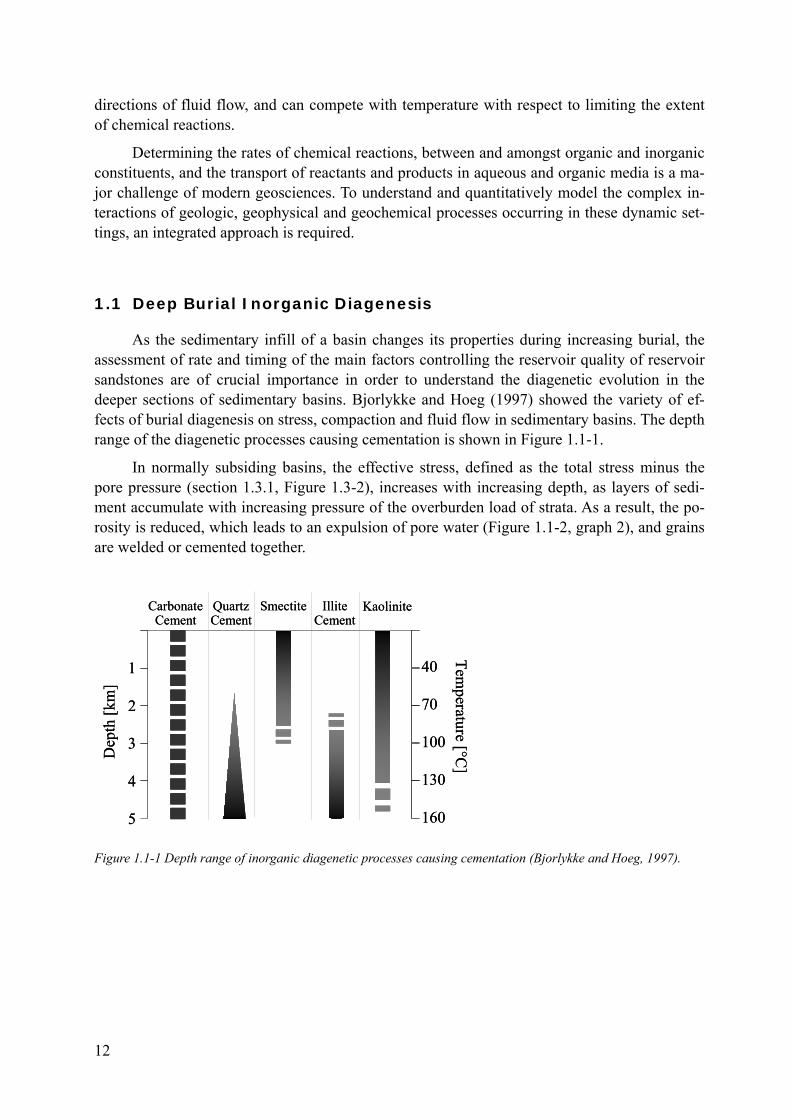
As the sedimentary infill of a basin changes its properties during increasing burial, the assessment of rate and timing of the main factors controlling the reservoir quality of reservoir sandstones are of crucial importance in order to understand the diagenetic evolution in the deeper sections of sedimentary basins. Bjorlykke and Hoeg (1997) showed the variety of ef-fects of burial diagenesis on stress, compaction and fluid flow in sedimentary basins. The depth range of the diagenetic processes causing cementation is shown in Figure 1.1-1.

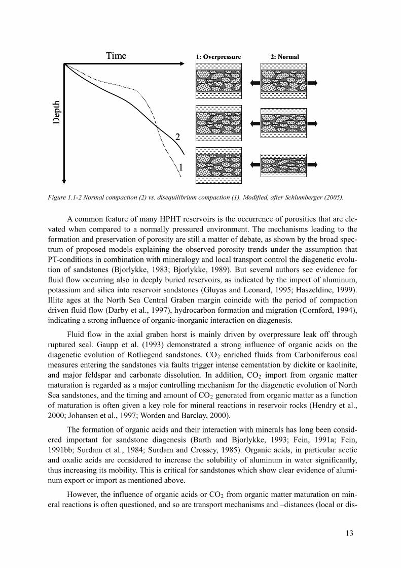
In normally subsiding basins, the effective stress, defined as the total stress minus the pore pressure (section 1.3.1, Figure 1.3-2), increases with increasing depth, as layers of sedi-ment accumulate with increasing pressure of the overburden load of strata. As a result, the po-rosity is reduced, which leads to an expulsion of pore water (Figure 1.1-2, graph 2), and grains are welded or cemented together.

1

2

3

4

5

Dep

th [k

m]

CarbonateCement

QuartzCement

Smectite IlliteCement

Kaolinite

40

70

100

130

160

Temperature [°C

]

1

2

3

4

5

Dep

th [k

m]

CarbonateCement

QuartzCement

Smectite IlliteCement

Kaolinite

40

70

100

130

160

Temperature [°C

]

Figure 1.1-1 Depth range of inorganic diagenetic processes causing cementation (Bjorlykke and Hoeg, 1997).

12

1: Overpressure 2: NormalTimeD

epth

1

2

1: Overpressure 2: NormalTimeD

epth

1

2

Figure 1.1-2 Normal compaction (2) vs. disequilibrium compaction (1). Modified, after Schlumberger (2005).

A common feature of many HPHT reservoirs is the occurrence of porosities that are ele-vated when compared to a normally pressured environment. The mechanisms leading to the formation and preservation of porosity are still a matter of debate, as shown by the broad spec-trum of proposed models explaining the observed porosity trends under the assumption that PT-conditions in combination with mineralogy and local transport control the diagenetic evolu-tion of sandstones (Bjorlykke, 1983; Bjorlykke, 1989). But several authors see evidence for fluid flow occurring also in deeply buried reservoirs, as indicated by the import of aluminum, potassium and silica into reservoir sandstones (Gluyas and Leonard, 1995; Haszeldine, 1999). Illite ages at the North Sea Central Graben margin coincide with the period of compaction driven fluid flow (Darby et al., 1997), hydrocarbon formation and migration (Cornford, 1994), indicating a strong influence of organic-inorganic interaction on diagenesis.

Fluid flow in the axial graben horst is mainly driven by overpressure leak off through ruptured seal. Gaupp et al. (1993) demonstrated a strong influence of organic acids on the diagenetic evolution of Rotliegend sandstones. CO2 enriched fluids from Carboniferous coal measures entering the sandstones via faults trigger intense cementation by dickite or kaolinite, and major feldspar and carbonate dissolution. In addition, CO2 import from organic matter maturation is regarded as a major controlling mechanism for the diagenetic evolution of North Sea sandstones, and the timing and amount of CO2 generated from organic matter as a function of maturation is often given a key role for mineral reactions in reservoir rocks (Hendry et al., 2000; Johansen et al., 1997; Worden and Barclay, 2000).

The formation of organic acids and their interaction with minerals has long been consid-ered important for sandstone diagenesis (Barth and Bjorlykke, 1993; Fein, 1991a; Fein, 1991bb; Surdam et al., 1984; Surdam and Crossey, 1985). Organic acids, in particular acetic and oxalic acids are considered to increase the solubility of aluminum in water significantly, thus increasing its mobility. This is critical for sandstones which show clear evidence of alumi-num export or import as mentioned above.

However, the influence of organic acids or CO2 from organic matter maturation on min-eral reactions is often questioned, and so are transport mechanisms and –distances (local or dis-

13

tant supply of reagents). Reactions occurring within the source rock may not leave reaction po-tential for the sandstones (e.g. Berger et al., 1997; Giles et al., 1994). Unrealistic high concen-trations are used in the experiments which are unlikely to occur in nature or complexing sites of organic acids may be occupied by other ions which are more abundant (Harrison and Thyne, 1994). This is discussed for aluminum which is almost insoluble in water but becomes several times more soluble through complexing by organic acids (Fein, 1991a; 1991bb).

As well as chemical reactions raising solubility significantly, transport mechanisms for dissolved species play a key role in the diagenetic evolution of rocks. The discussion continues as to whether closed system conditions without transport and cementation controlled by re-equilibrium of depositional mineralogy, (e.g. Bjorlykke et al., 1995), semi-closed system con-ditions with small-scale diffusional transport and a possible relationship between organic and inorganic diagenetic processes, (e.g. Gaupp et al., 1993), or open system conditions with large-scale fluid flow and a mass transport via exotic fluids (e.g. Haszeldine, 1999) are adequate de-scription of the diagenetic system.

There is plausible evidence from individual cases to support all three; no single system applies everywhere. The sample and data sets selected for the current study are representative for both open and closed system, as discussed later in the text (Figure 2.1-3, Section 2).

1.2 Predicting Petroleum Formation

Aside from being of economic focus, the petroleum itself can play an important role in the diagenetic evolution of the reservoir rocks in which it resides. By filling the reservoir with hydrocarbons via maturation and migration, certain mineral reactions are inhibited or even stopped, thus preserving porosity and permeability of the sandstone. While quartz cementation is not necessarily interrupted by oil migration (Brosse et al., 2000; Gluyas, 1997), illite forma-tion is hindered by the migration of oil or gas into the reservoir (Brosse et al., 2000; Gluyas and Leonard, 1995; Turner et al., 1993). But filling the reservoir with oil may also favor illiti-zation by reducing potassium mobility (Thyne et al., 2001).

The prediction of timing and spatial limits of hydrocarbon generation as well as its type, composition and quality are key tasks in petroleum exploration. When source rocks are buried, their macromolecular sedimentary organic matter is thermally degraded as a reaction to in-creasing thermal stress, and this process leads, over geological time, to the formation of hydro-carbons. The multitude of the chemical reactions involved in this process is in detail unknown, but considered irreversible (Schenk et al., 1997b).

Temperature is considered to be the driving force for the chemical reactions, leading to the transformation into hydrocarbons from the precursor kerogen. As an empirical rule of thumb, an increase of temperature of about 10°C was thought to more or less double the reac-tion rate, though this is well known to be highly variable (Quigley et al., 1987; Waples, 1983).

The kerogen type exerts a major influence on petroleum yield, type and timing of genera-tion (Poelchau et al., 1997), e.g. Type I kerogen is very likely to generate waxy oil, Type II kerogen can generate oil, and Type III kerogen is mainly considered gas-prone. The transfor-mation of kerogen to hydrocarbon is described through kinetic models of organic matter evolu-

14

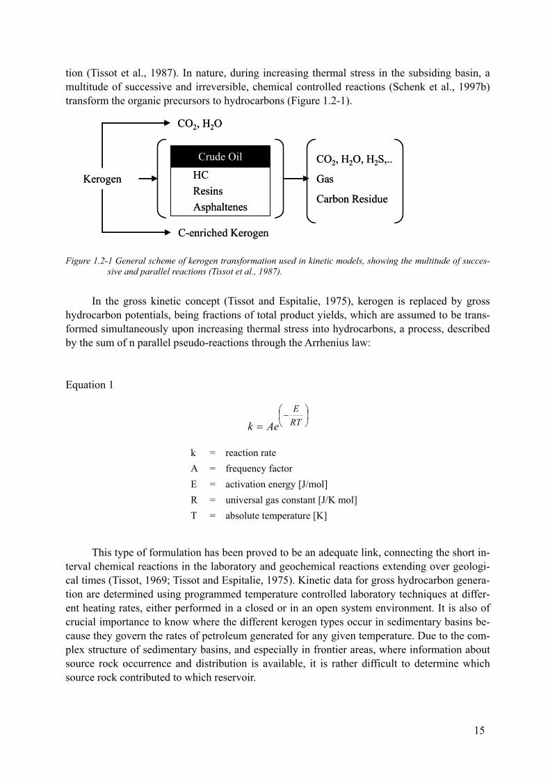
tion (Tissot et al., 1987). In nature, during increasing thermal stress in the subsiding basin, a multitude of successive and irreversible, chemical controlled reactions (Schenk et al., 1997b) transform the organic precursors to hydrocarbons (Figure 1.2-1).

C-enriched Kerogen

CO2, H2O

CO2, H2O, H2S,..

Gas

Carbon Residue

HCResinsAsphaltenes

Crude Oil

Kerogen

C-enriched Kerogen

CO2, H2O

CO2, H2O, H2S,..

Gas

Carbon Residue

HCResinsAsphaltenes

Crude Oil

Kerogen

Figure 1.2-1 General scheme of kerogen transformation used in kinetic models, showing the multitude of succes-sive and parallel reactions (Tissot et al., 1987).

In the gross kinetic concept (Tissot and Espitalie, 1975), kerogen is replaced by gross hydrocarbon potentials, being fractions of total product yields, which are assumed to be trans-formed simultaneously upon increasing thermal stress into hydrocarbons, a process, described by the sum of n parallel pseudo-reactions through the Arrhenius law:

Equation 1

⎟⎠⎞

⎜⎝⎛−

= RTE

Aek

k = reaction rate A = frequency factor E = activation energy [J/mol] R = universal gas constant [J/K mol] T = absolute temperature [K]

This type of formulation has been proved to be an adequate link, connecting the short in-terval chemical reactions in the laboratory and geochemical reactions extending over geologi-cal times (Tissot, 1969; Tissot and Espitalie, 1975). Kinetic data for gross hydrocarbon genera-tion are determined using programmed temperature controlled laboratory techniques at differ-ent heating rates, either performed in a closed or in an open system environment. It is also of crucial importance to know where the different kerogen types occur in sedimentary basins be-cause they govern the rates of petroleum generated for any given temperature. Due to the com-plex structure of sedimentary basins, and especially in frontier areas, where information about source rock occurrence and distribution is available, it is rather difficult to determine which source rock contributed to which reservoir.

15

Hydrocarbon generation has been studied in detail by various laboratory methods. Bulk kinetic methods describe the transformation of kerogen to petroleum. These methods, however, ignore compositional details and are therefore inapplicable for compositional prediction.

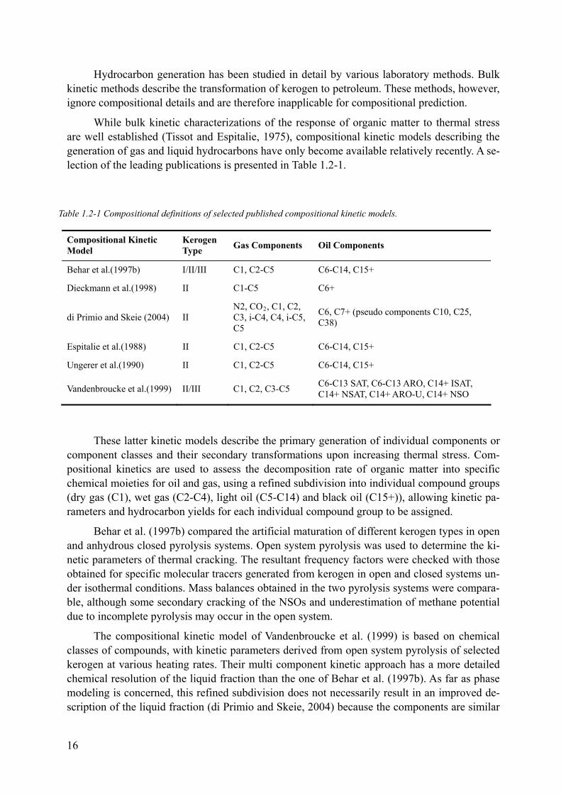
While bulk kinetic characterizations of the response of organic matter to thermal stress are well established (Tissot and Espitalie, 1975), compositional kinetic models describing the generation of gas and liquid hydrocarbons have only become available relatively recently. A se-lection of the leading publications is presented in Table 1.2-1.

Table 1.2-1 Compositional definitions of selected published compositional kinetic models.

Compositional Kinetic Model

Kerogen Type Gas Components Oil Components

Behar et al.(1997b) I/II/III C1, C2-C5 C6-C14, C15+

Dieckmann et al.(1998) II C1-C5 C6+

N2, CO2, C1, C2, C3, i-C4, C4, i-C5, C5

C6, C7+ (pseudo components C10, C25, C38) di Primio and Skeie (2004) II

Espitalie et al.(1988) II C1, C2-C5 C6-C14, C15+

Ungerer et al.(1990) II C1, C2-C5 C6-C14, C15+

C6-C13 SAT, C6-C13 ARO, C14+ ISAT, C14+ NSAT, C14+ ARO-U, C14+ NSO Vandenbroucke et al.(1999) II/III C1, C2, C3-C5

These latter kinetic models describe the primary generation of individual components or component classes and their secondary transformations upon increasing thermal stress. Com-positional kinetics are used to assess the decomposition rate of organic matter into specific chemical moieties for oil and gas, using a refined subdivision into individual compound groups (dry gas (C1), wet gas (C2-C4), light oil (C5-C14) and black oil (C15+)), allowing kinetic pa-rameters and hydrocarbon yields for each individual compound group to be assigned.

Behar et al. (1997b) compared the artificial maturation of different kerogen types in open and anhydrous closed pyrolysis systems. Open system pyrolysis was used to determine the ki-netic parameters of thermal cracking. The resultant frequency factors were checked with those obtained for specific molecular tracers generated from kerogen in open and closed systems un-der isothermal conditions. Mass balances obtained in the two pyrolysis systems were compara-ble, although some secondary cracking of the NSOs and underestimation of methane potential due to incomplete pyrolysis may occur in the open system.

The compositional kinetic model of Vandenbroucke et al. (1999) is based on chemical classes of compounds, with kinetic parameters derived from open system pyrolysis of selected kerogen at various heating rates. Their multi component kinetic approach has a more detailed chemical resolution of the liquid fraction than the one of Behar et al. (1997b). As far as phase modeling is concerned, this refined subdivision does not necessarily result in an improved de-scription of the liquid fraction (di Primio and Skeie, 2004) because the components are similar

16

in terms of their physical properties. Given the extremely high temperatures in their case study (HPHT Elgin Field, 190°C/110 MPa), it was rather unexpected that paraffinic condensates with nearly 50% n-C6+ alkanes were discovered, whereas only gas (n-C5−) was expected to be pre-sent. The predictions based on these compositional kinetic schemes showed that the content of methane was strongly underestimated compared to the actually observed methane content, while the condensed aromatics were severely overestimated. In addition, the GOR was also underestimated.

It must be taken into account that there is a systematic discrepancy in all laboratory heat-ing experiments, between gas compositions generated experimentally and those observed in nature. Methane content is distinctively higher in natural fluids (Mango, 1997), where the con-tent is actually wide spread. Propane and especially ethane contents are significantly elevated in the pyrolysates as compared to natural fluids. The extent of this discrepancy has been illus-trated in detail in di Primio and Skeie (2004) and later in di Primio and Horsfield (2006); it could explain in part the lack of methane in Vandenbroucke et al.’s 1999 prediction.

An additional reason for the overestimated ethane content could be related to the fact that the secondary cracking kinetics used were determined on a model compound (n-C25) pyro-lyzed under closed system conditions. Proving the correctness of secondary cracking predic-tions has been problematic (e.g. Vandenbroucke et al., 1999). For example the stability of liq-uid petroleum in reservoirs seems to be relatively high (Horsfield et al., 1992; Schenk and Horsfield, 1998; Schenk et al., 1997b), indicating that it can withstand temperatures close to 200°C under geologic heating rates, whereas in source rocks residual oil is converted to gas at lower levels of thermal stress (Dieckmann et al., 1998).

The kinetics of n-C25 cracking thus determined were very similar to those developed by Horsfield et al. (1992) and Schenk et al. (1997b) characterizing oil to gas cracking. As dis-cussed above, Dieckmann et al. (1998) showed that cracking of residual oil to gas in the source rock occurs significantly earlier. In addition, as compared to open system pyrolysis, GOR pre-dictions based on closed system pyrolysis including in-reservoir oil to gas cracking show a much better correlation to GORs observed in nature than those predictions achieved by open system heating experiments. In combination these observations indicate that reactions occur-ring within the source rock dominantly control the composition of petroleum in the reservoir. Only when the reservoir is isolated from further petroleum supply from the source can in-reservoir reactions dominantly influence the petroleum composition.

The more or less common occurrence of severely undersaturated, light oils or wet gas-condensates in the deep Central Graben of the North Sea is one similarity of HPHT reservoirs. As stated above, compositional predictions from kinetic models in combination with basin models have as yet large difficulties in correctly predicting the fluid composition and phase in deep, hot reservoirs (Vandenbroucke et al., 1999; Wendebourg, 2000). It seems likely that the problems encountered with hydrocarbon phase prediction in HPHT settings are due to either incorrect models of hydrocarbon expulsion or incorrect compositional kinetics when dealing with extreme pT-conditions.

The composition of generated petroleum changes during maturation, and so do, as a con-sequence, the physical properties of the migrating fluids, like GOR and API gravity. In order to predict these changes, a method is required (England and Mackenzie, 1989). Density, GOR and

17

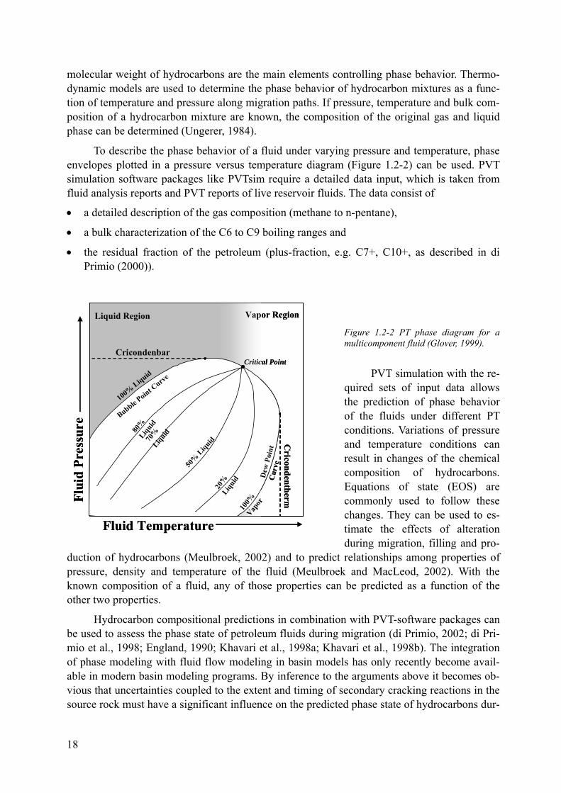
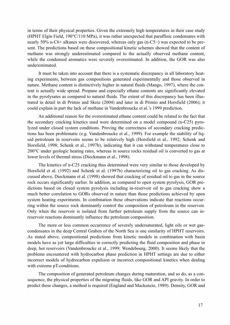
molecular weight of hydrocarbons are the main elements controlling phase behavior. Thermo-dynamic models are used to determine the phase behavior of hydrocarbon mixtures as a func-tion of temperature and pressure along migration paths. If pressure, temperature and bulk com-position of a hydrocarbon mixture are known, the composition of the original gas and liquid phase can be determined (Ungerer, 1984).

To describe the phase behavior of a fluid under varying pressure and temperature, phase envelopes plotted in a pressure versus temperature diagram (Figure 1.2-2) can be used. PVT simulation software packages like PVTsim require a detailed data input, which is taken from fluid analysis reports and PVT reports of live reservoir fluids. The data consist of

• a detailed description of the gas composition (methane to n-pentane),

• a bulk characterization of the C6 to C9 boiling ranges and

• the residual fraction of the petroleum (plus-fraction, e.g. C7+, C10+, as described in di Primio (2000)).

Figure 1.2-2 PT phase diagram for a multicomponent fluid (Glover, 1999).

PVT simulation with the re-quired sets of input data allows the prediction of phase behavior of the fluids under different PT conditions. Variations of pressure and temperature conditions can result in changes of the chemical composition of hydrocarbons. Equations of state (EOS) are commonly used to follow these changes. They can be used to es-timate the effects of alteration during migration, filling and pro-

duction of hydrocarbons (Meulbroek, 2002) and to predict relationships among properties of pressure, density and temperature of the fluid (Meulbroek and MacLeod, 2002). With the known composition of a fluid, any of those properties can be predicted as a function of the other two properties.

Liquid Region

Cricondenbar

Cricondentherm

Critical Point

100% Liquid

Bubble Point C

urve

Dew

Poi

nt

Cur

ve

80%

Liqu

id

20%

Liqu

id

70%

Liqu

id

50%

Liquid

Fluid Temperature

Flui

d Pr

essu

re

100%

Vap

or

Vapor RegionLiquid Region

Cricondenbar

Cricondentherm

Critical Point

100% Liquid

Bubble Point C

urve

Dew

Poi

nt

Cur

ve

80%

Liqu

id

20%

Liqu

id

70%

Liqu

id

50%

Liquid

Fluid Temperature

Flui

d Pr

essu

re

100%

Vap

or

Vapor Region

Hydrocarbon compositional predictions in combination with PVT-software packages can be used to assess the phase state of petroleum fluids during migration (di Primio, 2002; di Pri-mio et al., 1998; England, 1990; Khavari et al., 1998a; Khavari et al., 1998b). The integration of phase modeling with fluid flow modeling in basin models has only recently become avail-able in modern basin modeling programs. By inference to the arguments above it becomes ob-vious that uncertainties coupled to the extent and timing of secondary cracking reactions in the source rock must have a significant influence on the predicted phase state of hydrocarbons dur-

18

ing secondary migration, and that in-reservoir processes attributable to phase separation (as-phaltene precipitation, gas flushing) will be incorrectly modeled.

A broad spectrum of compositional kinetic models is available today (e.g. Behar et al., 1997b; Dieckmann et al., 1998; Pepper and Corvi, 1995a, b; Vandenbroucke et al., 1999), but despite the fact that the possibility to model the phase behavior of fluids during migration is nowadays integrated in commercial basin modeling software, only a single compositional ki-netic model which has been demonstrated to correctly reproduce fluid phase behavior, has been published to date (di Primio and Skeie, 2004).

A similar model was presented by di Primio and Horsfield (2006). Their model is based on four sequential stages, the first being the definition of the petroleum type organic facies, based on the classification scheme of Horsfield (1989), which uses the petroleum composition to define the organofacies type. The model uses a combination of open and closed system pyro-lysis techniques to characterize the compositional evolution of the fluids generated as a func-tion of increasing thermal stress. Gas compositions determined analytically are tuned to natural fluid phase behavior by adjusting the pyrolysates gas compositions empirically by assuming increasing ratios of methane to wet gas compounds. The ensuing “corrected” gas compositions used for the definition of multi-compound kinetic models. Such methods represent the state of the art in the definition of compositional kinetic – phase predictive models; they are, however, also limited to the range of primary cracking.

One goal of this study was to extend such existing models to include light oil and gas condensate formation, which are commonly encountered in HPHT settings.

19

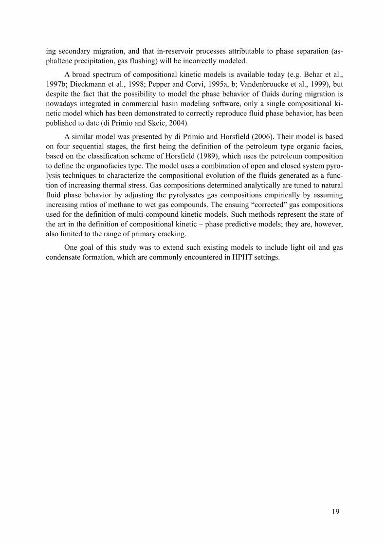
1.3 HPHT Settings

Overpressured rocks are typical features of many sedimentary basins worldwide (Figure 1.3-1). They occur in a wide range of geological conditions, more frequently within young Ter-tiary basins from about 1-2 km downwards, but also in older Mesozoic reservoirs (Swarbrick, 1998).

0

50

100

150

200

250

0 25 50 75 100 125

Initial Reservoir Pressure [MPa]

Res

ervo

ir T

empe

ratu

re [°

C]

North SeaGulf of MexicoOther

normal gradientHPHT lower limits

Central North Sea Graben System

Gulf of Mexico

0

50

100

150

200

250

0 25 50 75 100 125

Initial Reservoir Pressure [MPa]

Res

ervo

ir T

empe

ratu

re [°

C]

North SeaGulf of MexicoOther

normal gradientHPHT lower limits

Central North Sea Graben System

Gulf of Mexico

Figure 1.3-1 HPHT well locations and -reservoir pT conditions worldwide, including normal pT gradient. HPHT wells are concentrated in the Gulf of Mexico and in the North Sea (modified, after Adamson et al., 1998).

Wells having undisturbed bottomhole temperature at and above 150°C are classified as high temperature wells. Those wells having pore pressure gradients of at least 18 kPa/m or those requiring a blowout preventer with a rating in excess of 68.95 MPa are classed as high pressure wells. Wells meeting both criteria are formally defined as HPHT wells. Fields reach-

20

ing HPHT conditions must be regarded as out of equilibrium, because of the transitory charac-ter of abnormally high pressures. Such fields can exist widely, but they need to survive tectonic stresses which may rupture their seals. Overpressured reservoirs cannot be expected to be super major fields because seals are not likely to be maintained over very large areas. High gas con-tent fluids are to be expected due to the partial cracking of large molecules at past high tem-peratures (Barker, 1990).

HPHT fields have been successfully developed since the nineteen seventies, like the Thomasville HPHT field, located in the eastern Gulf of Mexico region, onshore Mississippi. However, it was the disaster of the Piper Alpha platform in the UK sector of the North Sea in 1988, along with the contemporaneous loss of the Ocean Odyssey drilling vessel in Scottish ju-risdictional waters (EERTAG, 1997), and the following release of the Cullen report, which demonstrated the hazardous nature and the technical challenge of those areas. Despite the tech-nical challenge of exploring for HPHT fields, activity has moved more and more in this direc-tion, especially towards the extremely overpressured regions of the Gulf of Mexico and the North Sea’s graben system.

In terms of the dynamic of subsurface fluid flow, overpressure is the result of the inabil-ity of formation fluids to escape at a rate which allows equilibration with hydrostatic pressure (Swarbrick, 1998). The amount and build-up rate of overpressure is directly controlled by the permeability of the lateral and vertical non-reservoir sealing rocks, following thereby Darcy’s Law, which is defined as the relationship for the fluid flow rate q through a porous medium:

Equation 2

xpkAq

ΔΔ

= *μ

k = permeability

A = cross-sectional area

µ = viscosity

∆p = pressure difference across the distance ∆x

In the case of a low permeable sealing rock only small amounts of fluid will be able to leave an overpressured cell, further pressure build-up will therefore occur as long as new fluids are entering the cell. Because shales and clays can act as membranes, osmotic pressures may occur in the subsurface (Fritz, 1983), but due to the heterogeneity of these lithologies, they can not be defined as ideal membranes, and the contribution of osmotic phenomena to overpressure is therefore widely regarded as negligible (Swarbrick, 1998).

Seal failure as a result of fracturing may reduce overpressure. Fractures can be due to the reactivation of faults in tectonic active regions (Byerlee, 1993) or continued pressure buildup without release within the reservoir. Hydraulic fracturing of the sealing rock occurs, when the fluid pressure is so high that the tension stresses surpass the cohesive strength of the rock

21

(Bjorlykke and Hoeg, 1997); the pore pressure distribution in the overpressured areas of the North Sea is controlled to a large degree by hydrofracturing of pressure seals. Gas chimneys overlying overpressured areas often indicate vertical migration of hydrocarbons following seal fracture (Buhrig, 1989). Fluid leakage is caused by those pressure-induced fractures, followed by a pressure loss or equilibration within the overpressured cell, resulting in recalibration of the reservoir fluid’s chemistry and pressure conditions. In most cases, open fractures are only tem-porary features; with time they will be closed by mechanical deformation or become cemented by precipitated minerals. The cementation of fractures by carbonate cements may occur at any given depth. Cements may be derived by diffusion from the matrix or by transport of water along the fractures (Bjorlykke and Hoeg, 1997). The following resealing of the fracture will induce new pressure build-up (Ward, 1994).

1.3.1 North Sea, Central Graben: HPHT-zone

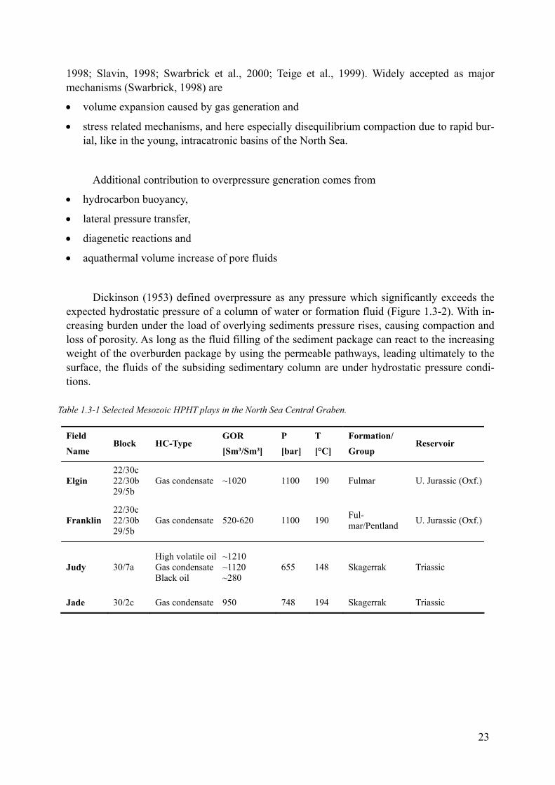
The deep Triassic and Jurassic plays of the HPHT zone studied here consist of deep gas condensates within reservoirs where pore pressures approach lithostatic conditions (Holm, 1998). Reservoir pressures exceeding 690 bar and high temperatures of more than 150°C are typical features for many of the Central North Sea’s Mesozoic reservoirs, especially those within the Central Graben (Table 1.3-1).

Dickinson (1953) defined overpressure as any pressure which significantly exceeds the expected hydrostatic pressure of a column of water or formation fluid (Figure 1.3 2). With in-creasing burden under the load of overlying sediments pressure rises, causing compaction and loss of porosity. As long as the fluid filling of the sediment package can react to the increasing weight of the overburden package by using the permeable pathways, leading ultimately to the surface, the fluids of the subsiding sedimentary column are under hydrostatic pressure condi-tions.

Darby et al.(1996) defines a pressure cell as a body of rock containing overpressured flu-ids that are internally in free hydraulic communication. Top, bottom and lateral pressure seals are restricting the free fluid flow between pressure cells (Holm, 1998). Two distinct pressure domains dominate the Central Graben area, separated by a low porosity (< 5%) pressure seal within the Upper Cretaceous Chalk Group (Ward, 1994). This stratigraphicaly independent pressure seal occurs in a depth of about 3.5-4km. An increase of depth occurs towards the gra-ben margins, where the geothermal gradient is lower (Leonard, 1993). The Mesozoic sediments below this depth are under overpressured conditions. Apparently there is no common HC-water contact across the fields (Swarbrick et al., 2000). In addition, Darby et al. (1996) characterized the Kimmeridge Clay Formation as a pressure seal in deep terraces. Where Jurassic formations are absent, the basal Upper Cretaceous Hod Formation of the Chalk Group forms the upper seal of the overpressured cell. The lateral seals are faults, proven by differences between HC-water contacts and variations in the GOR, despite sand to sand contacts on the intervening faults (ConocoPhillips, pers. comm.).

The mechanisms of overpressure generation in the North Sea area are still subject of de-bate (Bolas et al., 2004; Borge, 1999; Darby et al., 1996; Gaarenstroom et al., 1993; Holm,

22

1998; Slavin, 1998; Swarbrick et al., 2000; Teige et al., 1999). Widely accepted as major mechanisms (Swarbrick, 1998) are

• volume expansion caused by gas generation and

• stress related mechanisms, and here especially disequilibrium compaction due to rapid bur-ial, like in the young, intracatronic basins of the North Sea.

Additional contribution to overpressure generation comes from

• hydrocarbon buoyancy,

• lateral pressure transfer,

• diagenetic reactions and

• aquathermal volume increase of pore fluids

Dickinson (1953) defined overpressure as any pressure which significantly exceeds the expected hydrostatic pressure of a column of water or formation fluid (Figure 1.3-2). With in-creasing burden under the load of overlying sediments pressure rises, causing compaction and loss of porosity. As long as the fluid filling of the sediment package can react to the increasing weight of the overburden package by using the permeable pathways, leading ultimately to the surface, the fluids of the subsiding sedimentary column are under hydrostatic pressure condi-tions.

Table 1.3-1 Selected Mesozoic HPHT plays in the North Sea Central Graben.

Field GOR P T Formation/ Block HC-Type Reservoir

Name [Sm³/Sm³] [bar] [°C] Group

22/30c 22/30b 29/5b

Elgin Gas condensate ~1020 1100 190 Fulmar U. Jurassic (Oxf.)

22/30c 22/30b 29/5b

Ful-mar/Pentland Franklin Gas condensate 520-620 1100 190 U. Jurassic (Oxf.)

High volatile oil Gas condensate Black oil

~1210 ~1120 ~280

Judy 30/7a 655 148 Skagerrak Triassic

Jade 30/2c Gas condensate 950 748 194 Skagerrak Triassic

23

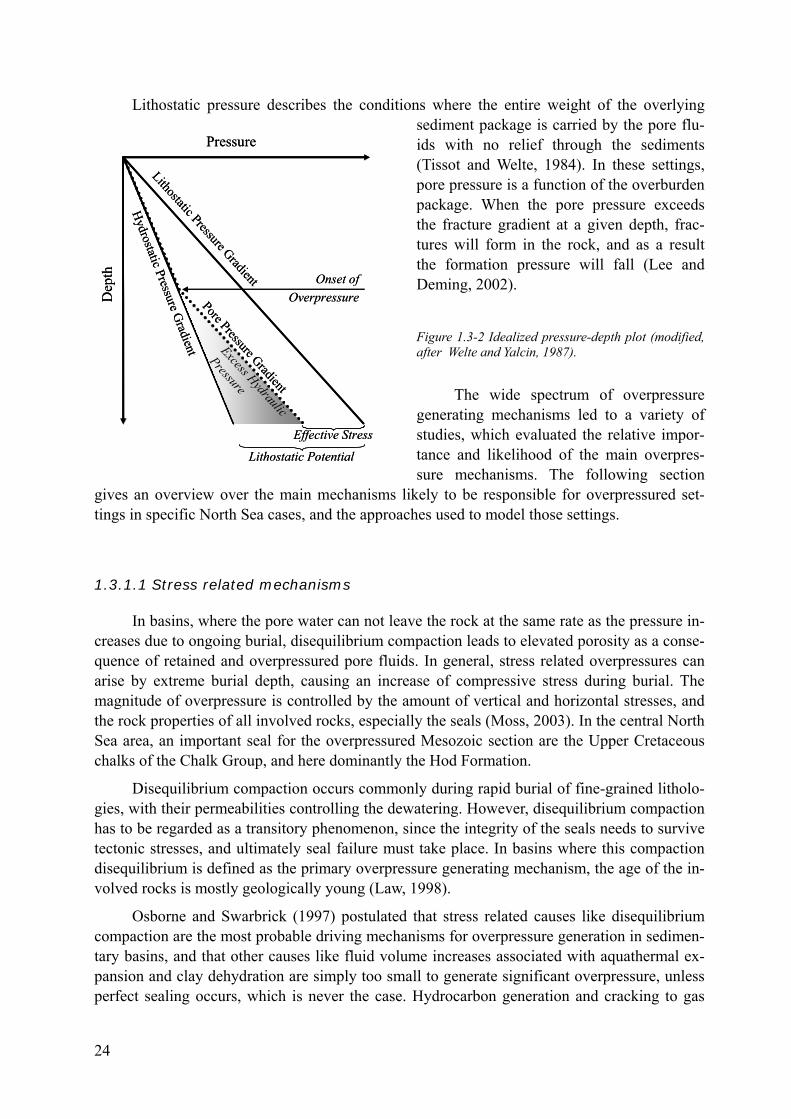
Lithostatic pressure describes the conditions where the entire weight of the overlying sediment package is carried by the pore flu-ids with no relief through the sediments (Tissot and Welte, 1984). In these settings, pore pressure is a function of the overburden package. When the pore pressure exceeds the fracture gradient at a given depth, frac-tures will form in the rock, and as a result the formation pressure will fall (Lee and Deming, 2002).

Figure 1.3-2 Idealized pressure-depth plot (modified, after Welte and Yalcin, 1987).

The wide spectrum of overpressure generating mechanisms led to a variety of studies, which evaluated the relative impor-tance and likelihood of the main overpres-sure mechanisms. The following section

gives an overview over the main mechanisms likely to be responsible for overpressured set-tings in specific North Sea cases, and the approaches used to model those settings.

Pressure

Dep

th

Hydrostatic Pressure G

radient

Lithostatic Pressure Gradient

Pore Pressure Gradient

Onset ofOverpressure

Lithostatic Potential

Effective Stress

Excess Hydraulic

Pressure

Pressure

Dep

th

Hydrostatic Pressure G

radient

Lithostatic Pressure Gradient

Pore Pressure Gradient

Onset ofOverpressure

Lithostatic Potential

Effective Stress

Excess Hydraulic

Pressure

1.3.1.1 Stress related mechanisms

In basins, where the pore water can not leave the rock at the same rate as the pressure in-creases due to ongoing burial, disequilibrium compaction leads to elevated porosity as a conse-quence of retained and overpressured pore fluids. In general, stress related overpressures can arise by extreme burial depth, causing an increase of compressive stress during burial. The magnitude of overpressure is controlled by the amount of vertical and horizontal stresses, and the rock properties of all involved rocks, especially the seals (Moss, 2003). In the central North Sea area, an important seal for the overpressured Mesozoic section are the Upper Cretaceous chalks of the Chalk Group, and here dominantly the Hod Formation.

Disequilibrium compaction occurs commonly during rapid burial of fine-grained litholo-gies, with their permeabilities controlling the dewatering. However, disequilibrium compaction has to be regarded as a transitory phenomenon, since the integrity of the seals needs to survive tectonic stresses, and ultimately seal failure must take place. In basins where this compaction disequilibrium is defined as the primary overpressure generating mechanism, the age of the in-volved rocks is mostly geologically young (Law, 1998).

Osborne and Swarbrick (1997) postulated that stress related causes like disequilibrium compaction are the most probable driving mechanisms for overpressure generation in sedimen-tary basins, and that other causes like fluid volume increases associated with aquathermal ex-pansion and clay dehydration are simply too small to generate significant overpressure, unless perfect sealing occurs, which is never the case. Hydrocarbon generation and cracking to gas

24

could possibly produce overpressure, but these processes may be self-limiting in a sealed sys-tem because buildup of pressure could inhibit further organic maturation, but maturity retarda-tion or suppression is a matter of debate, still with ambiguous results. While it is well estab-lished that the evolution of maturity indicators like vitrinite reflectance is controlled by tem-perature and time and that factors like fluid chemistry, pressure and others play only minor roles for the evolution of maturation, some workers indeed see a connection between overpres-sure and the retardation of vitrinite maturation (Carr, 1999; Carr, 2000; Torre et al., 1997; Zou and Peng, 2001). The retardation of vitrinite maturation refers to a thermomechanical decrease in reaction rate as an outcome of overpressure in sedimentary basins (Carr, 2000). Within over-pressured settings, retardation can appear below the pressure seal and is maintained as long as overpressure continues. Identification of maturity retardation is crucial for basin modeling, as non-observance may lead to misconstruction of the thermal history of source rocks.

Swarbrick et al. (2000) studied the overpressured settings and petroleum filling history in the Triassic reservoirs of the Judy Field, located within the study area of this thesis in the Cen-tral Graben, using 2D basin modeling. To match measured pressure data with modeled values, the default permeabilities of the major seal, basically chalks (Chalk Group), were iteratively adjusted, because fine-grained lithologies are often poorly characterized and the term “shale” and “chalk” actually encompasses a wide range of sediments that compact in different ways, depending on their particular grain size distribution. As a consequence, several effective stress-porosity and porosity-permeability functions were developed (Yardley and Swarbrick, 2000). In addition, average chalk permeability and compaction behavior for non-reservoir chalks are major points of uncertainty, as published data are biased to the reservoir intervals (Scholle, 1977). The data used in the study of the Judy Field was calibrated to palaeo-pressure data ob-tained from fluid inclusions. Their results showed that disequilibrium compaction due to rapid Quaternary burial is the driving force for overpressure development in the Judy Field, with only small contribution from additional sources like gas generation and lateral pressure transfer (Swarbrick et al., 2000).

Enhanced porosities are not always a characteristic feature of overpressured settings, which supports the assumption that disequilibrium compaction is not the only overpressure generating mechanism. Teige et al. (1999) showed that in the overpressured Haltenbanken area that shales failed to show elevated porosities. On the contrary, each formation seems to have been individually compacted according to burial depth, independent of pressure regimes. A similar observation was made by Bolas et al. (2004) in a basin modeling study performed in the Gullfaks Field in the North Sea, using fluid-flow simulations and porosity modeling to evaluate the existence of porosity vs. effective stress relationships in shales. Data showed that overpressured shales in the North Sea do not necessarily show elevated porosities as compared to the normally pressured shales of the same formation at similar depths. Here, results indi-cated that effective stress-driven compaction alone has not generated the hard overpressures observed in deeply buried North Sea shales, which means that the importance of disequilibrium compaction is, at least in the settings studied, overestimated.

However, the overpressure and seal development in the Central Graben area is very com-plex to the extent that every individual pressure cell including the regional pressure seal of the Cretaceous Hod Formation have different fill and spill routes.

25

1.3.1.2 Volume changes of the pore fluids

Thermal expansion as a reaction of fluids to increasing temperatures in a closed system is regarded as an effective overpressure generating mechanism. Increasing temperatures can be induced by increasing burial depth of the reservoir or downward migration of fluids into areas of higher temperature. However, experiments and modeling suggest that aquathermal induced overpressure is only of significance if permeabilities tend towards zero (Barker, 1972; Barker et al., 1978; Luo, 1992). Nevertheless thermal expansion of fluids contributes additional pres-sure to existing overpressure system.

Gas generation seems to be a significant reason for the generation of overpressure. Rising temperature causes a conversion of oil into thermal gas. The cracking of oil and bitumen to gas under geological heating rates (e. g. 5K/Ma) occurs within a temperature range of about 180°-225°C for high wax oils; for marine oils the onset of gas generation is predicted to be at about 170°C. Oil-togas cracking is unlikely to take place at temperatures less than 160°C, whatever the crude oil type or the geological heating rate (Schenk et al., 1997a). Pressure increase ac-companies this process, assuming the system is closed. At standard pT conditions, approxi-mately 85 m³ of gas is generated from one barrel of oil, as a result of thermal cracking from oil to gas upon increasing depth and temperatures (Barker, 1990). Barker demonstrated that in an isolated system the lithostatic pressure gradient is reached after only 1% of the reservoired oil is converted to gas.

The Anadarko basin, which covers almost the entire western part of Oklahoma and some parts of Kansas, Texas and Colorado, is an example for a large and deep Paleozoic basin, with the most strata ranging from Cambrian to Permian. The basin is petroleum rich and well ex-plored. Lee and Deming (2002) evaluated here the relative importance of disequilibrium com-paction and gas generation, using scale analysis and 1D numerical modeling. They showed that to explain the overpressured settings in this basin purely by disequilibrium compaction unlikely low permeabilities (10-12 mD) for the pressure seals must be defined, while gas gen-eration as major overpressure contributor would require distinctively lower permeabilities for the seals (<10-8 mD). However, a limitation of this study is that currently pressure seal proper-ties in that basin, which could help to verify the study’s results, are unknown.

Buhrig (1989) analyzed the formation pressure data from Jurassic and Triassic reservoirs of 192 wells in the Norwegian and UK sector in the Viking Graben, North Sea, and distin-guished several different pressure regimes: An open system consisting of normally pressured reservoirs, a ‘restricted system’ containing strata showing pressures above the hydrostatic pres-sure gradient, interpreted to be in partial pressure communication with the open system through lateral or vertical pressure drainage, and a ‘closed system’ containing highly overpressured res-ervoirs. The latter was assumed to be a representative case for the variety of overpressure mechanisms being active, disequilibrium compaction, aquathermal pressuring, oil generation and possibly by shale dewatering above the depth for the onset of gas generation (formation overpressure typically in the range 10-17 MPa). Gas generation is interpreted to be a major overpressure contributor below that depth (formation overpressure higher than 20 MPa). In the former case, a pore pressure gradient approximately 50% higher than the hydrostatic gradient is estimated. In the latter case, a much more drastic overpressure increase with depth is sug-gested.

26

Isaksen (2004) studied the hydrocarbon systems in the Central North Sea HPHT area in order to improve current understanding of oil and gas compositional histories in HPHT hydro-carbon systems. In this area, several oil accumulations are said to have undergone in-reservoir thermal cracking, resulting in a lighter, single-phase fluid, together with a pyrobitumen residue in the pore volumes. The integrated study of the hydrocarbon system with emphasis on detailed petroleum geochemistry showed that the main causes of pressure increase in the Mesozoic sedimentary sequences are thought to be volume increase associated with gas generation from source rocks, clay dehydration, and thermal cracking of oil, all of them being controlled by the rapid Quaternary burial, which had a direct impact on the thermal regime and the extent of in-situ thermal cracking of oil in the HPHT fields.

1.3.1.3 Other

Diagenetic reactions are assumed to contribute to the cumulated amount of overpressure in sedimentary basins (Bruce, 1984), as pore volume cementation reduces the pore volume (Osborne and Swarbrick, 1999). Mixed layer clay minerals such as smectite can adsorb water molecules due to their negative charge (Matthes, 1993). With increasing p-T conditions, Al- and K-ions replace Na, Ca, Mg, Fe, Si and H2O in clay minerals, the product is illite, having a reduced ability to adsorb water. Clay dehydration is the release of bound water during the al-teration of smectite to illite, a process which might cause an increase of the fluid volume. In a study of overpressured Upper Jurassic clastic reservoirs of the Fulmar formation in the Central North Sea, theoretical calculations showed that diagenetic reactions occurring in the overpres-sured reservoir (smectite illitisation and quartz cementation), did not generate significant over-pressure, because seal permeabilities were too high and the rate of volume increase associated with the reactions too small (Osborne and Swarbrick, 1999). Based on those results, the au-thors inferred that diagenetic reactions can effectively be ignored when modeling overpressure generation in the Central North Sea, although cementation will affect rock permeability and rates of fluid dissipation (Osborne and Swarbrick, 1999).

Lateral pressure transfer plays a significant role when dealing within overpressured set-tings. Borge (2002) developed a pressure simulator (Pressim), which uses a pressure compart-ment methodology to model lateral pressure transfer by describing the 3D fluid flow pattern within the basin on a geological time scale. The model includes mechanical compaction and quartz cementation as pressure generating processes. The methodology is based on the assump-tion that low permeable faults divide the basin into pressure compartments, with shales as up-per and lower boundaries. Calibration was done by adjusting the transmissibility of the faults, which act as pressure boundaries. This approach reduces the need for user defined poro-perm relationships or porosity-depth trends. The methodology was tested in the Halten Terrace area, offshore Norway. The results indicate, that the main proportion of overpressure is due to me-chanical shale compaction, coupled with chemical compaction and quartz cementation, but to a high degree being controlled by the integrity of the faults and thus by lateral pressure transfer. Because of the wide spectrum of overpressure generating mechanisms as listed above, the ex-act determination of the cause or causes is often difficult, as is the way to model overpressure. In all probability it is not one mechanism alone leading to HPHT conditions, but a combination of different mechanisms.

27

1.4 Problems and Objectives

The FLINT project (Mineral-Fluid Interactions) belonging to the program

“Dynamik sedimentärer Systeme unter wechselnden Spannungsregimen am Beispiel des zentraleuropäischen Beckensystems“

of the Deutsche Forschungsgemeinschaft (German Research Foundation, DFG) was ini-tiated to address the questions raised in the preceding discussions. Its goals were to reconstruct the diagenetic evolution of the reservoir rocks and the compositional evolution of the reservoir fluids, as well as investigating the interactions between the two, in the HPHT settings of the Central Graben. Organic geochemistry and numerical modeling of the basin were chosen as in-vestigative tools.

For a complete understanding of the diagenetic evolution of reservoir sandstones the tim-ing of hydrocarbon generation and migration as well as the characterization of hydrocarbon phase should not be neglected. Under certain conditions, hydrocarbon emplacement can even be the dominant factor controlling porosity and permeability of the rocks. The mechanism of emplacement of aqueous pore fluids by hydrocarbons which will inhibit diagenetic reactions is generally accepted. Porosity and permeability of a reservoir can be preserved if the reservoir is charged with oil during early burial (Burley, 1993).

For this reason, both the integration of basin modeling to predict hydrocarbon formation and migration, and the determination of aqueous flow rates were central parts of this project. The combination of the results obtained in this study, with those of reactive-transport modeling (done by Dr. Robert Ondrak, GFZ-Potsdam) and petrographic studies (Dipl.Geol. Robert Lippmann, Friedrich-Schiller University, Jena) helped to develop a good understanding of the processes and dynamics controlling the system.

This thesis sets out to reproduce the evolution of the reservoir fluids, both with respect to their compositions as well as the corresponding physical properties (GOR, API) and the tempo-ral and spatial limits of hydrocarbon generation.

28

2 The Study Area

2.1 Regional Settings

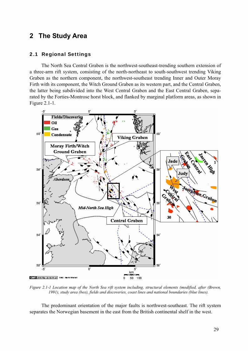
The North Sea Central Graben is the northwest-southeast-trending southern extension of a three-arm rift system, consisting of the north-northeast to south-southwest trending Viking Graben as the northern component, the northwest-southeast trending Inner and Outer Moray Firth with its component, the Witch Ground Graben as its western part, and the Central Graben, the latter being subdivided into the West Central Graben and the East Central Graben, sepa-rated by the Forties-Montrose horst block, and flanked by marginal platform areas, as shown in Figure 2.1-1.

Figure 2.1-1 Location map of the North Sea rift system including, structural elements (modified, after (Brown, 1991), study area (box), fields and discoveries, coast lines and national boundaries (blue lines).

The predominant orientation of the major faults is northwest-southeast. The rift system separates the Norwegian basement in the east from the British continental shelf in the west.

29

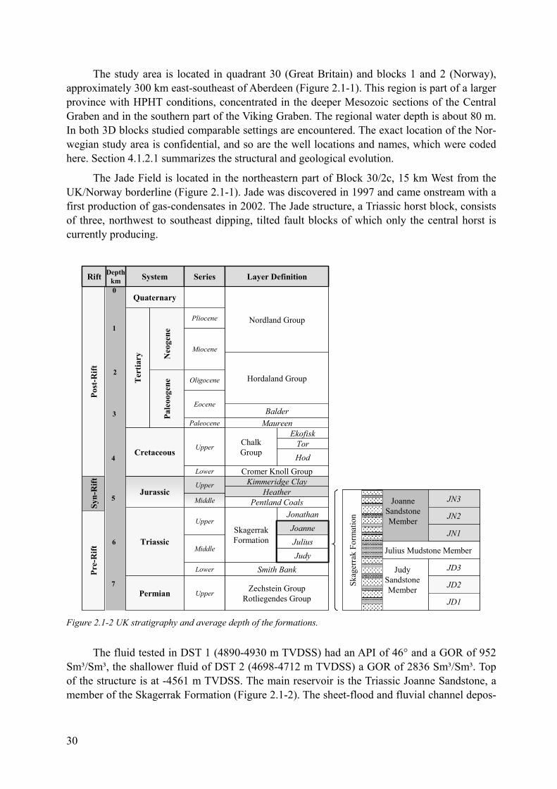
The study area is located in quadrant 30 (Great Britain) and blocks 1 and 2 (Norway), approximately 300 km east-southeast of Aberdeen (Figure 2.1-1). This region is part of a larger province with HPHT conditions, concentrated in the deeper Mesozoic sections of the Central Graben and in the southern part of the Viking Graben. The regional water depth is about 80 m. In both 3D blocks studied comparable settings are encountered. The exact location of the Nor-wegian study area is confidential, and so are the well locations and names, which were coded here. Section 4.1.2.1 summarizes the structural and geological evolution.

The Jade Field is located in the northeastern part of Block 30/2c, 15 km West from the UK/Norway borderline (Figure 2.1-1). Jade was discovered in 1997 and came onstream with a first production of gas-condensates in 2002. The Jade structure, a Triassic horst block, consists of three, northwest to southeast dipping, tilted fault blocks of which only the central horst is currently producing.

System Series Layer Definition

Quaternary

Ter

tiary N

eoge

nePa

leoo

gene

Pliocene

Miocene

Oligocene

Eocene

Paleocene

CretaceousUpper

Lower

JurassicUpper

Middle

Triassic

Upper

Middle

Lower

Kimmeridge ClayHeather

Pentland Coals

Smith Bank

SkagerrakFormation

JonathanJoanneJuliusJudy

Post

-Rift

Syn-

Rift

Pre-

Rift

Rift

Cromer Knoll Group

ChalkGroup

TorHod

EkofiskMaureenBalder

Hordaland Group

Nordland Group

Permian Upper Zechstein GroupRotliegendes Group

1

3

2

0

5

7

6

4

Depthkm

JoanneSandstoneMember

JN3

JN2

JN1

Julius Mudstone Member

JudySandstoneMember

JD3

JD2

JD1

Skag

erra

k Fo

rmat

ion

System Series Layer Definition

Quaternary

Ter

tiary N

eoge

nePa

leoo

gene

Pliocene

Miocene

Oligocene

Eocene

Paleocene

CretaceousUpper

Lower

JurassicUpper

Middle

Triassic

Upper

Middle

Lower

Kimmeridge ClayHeather

Pentland Coals

Smith Bank

SkagerrakFormation

JonathanJoanneJuliusJudy

Post

-Rift

Syn-

Rift

Pre-

Rift

Rift

Cromer Knoll Group

ChalkGroup

TorHod

EkofiskMaureenBalder

Hordaland Group

Nordland Group

Permian Upper Zechstein GroupRotliegendes Group

1

3

2

0

5

7

6

4

Depthkm

JoanneSandstoneMember

JN3

JN2

JN1

Julius Mudstone Member

JudySandstoneMember

JD3

JD2

JD1

Skag

erra

k Fo

rmat

ion

JoanneSandstoneMember

JN3

JN2

JN1

Julius Mudstone Member

JudySandstoneMember

JD3

JD2

JD1

Skag

erra

k Fo

rmat

ion

Figure 2.1-2 UK stratigraphy and average depth of the formations.

The fluid tested in DST 1 (4890-4930 m TVDSS) had an API of 46° and a GOR of 952 Sm³/Sm³, the shallower fluid of DST 2 (4698-4712 m TVDSS) a GOR of 2836 Sm³/Sm³. Top of the structure is at -4561 m TVDSS. The main reservoir is the Triassic Joanne Sandstone, a member of the Skagerrak Formation (Figure 2.1-2). The sheet-flood and fluvial channel depos-

30

its of the Joanne Sandstone Member reach a thickness of 70-490 m (average 400 m) with a good to excellent reservoir quality (average porosity of 17%; permeability > 100-2000 mD), which is predominantly facies controlled with the most effective reservoirs developed in chan-nel sands (Fisher and Mudge, 1998). Zonal boundaries, which are often associated with promi-nent lacustrine mudstone horizons, are locally well defined, as reported in internal studies from ConocoPhillips. The Joanne Sandstone is subdivided into six sandstone packages with shaly in-terbeds. The Jade structure is described in detail by Jones (2004).

The reservoir is under HPHT conditions, as indicated by reservoir temperatures reaching above 180°C (DST data), and pressures well above 80 MPa. The sealing chalks of the Hod Formation overlie the Joanne Sandstone. All three source rock units,

• the Kimmeridge Clay Formation,

• the Heather Formation and

• the Pentland Formation,

are absent at the top of the structure, but are present in the neighboring deeper basin in the Southeast, the kitchen area for the Jade structure.

The second producing field under study is Judy, located in a horst structure approxi-mately 19 km south of Jade in Block 30/7a. It was discovered in 1985, and is producing a mix-ture of low GOR and high volatile oils plus gas condensates (40-42 °API; GOR 500-1000 Sm³/Sm³). The field has been described in detail by Swarbrick et al. (2000). The reservoir unit is the Triassic Judy Sandstone (Figure 2.1-2), a stratigraphically older member of the Skager-rak Formation, with temperatures up to 145°C at -3400 m TVDSS and pressures reaching 60 MPa. At the top of the Triassic reservoir, a thin layer of the Kimmeridge Clay Formation is present, overlain by the pressure seals of the Chalk Group. The geologic settings, thermal and pressure history and the burial history are very similar to those of the Jade Field described above.

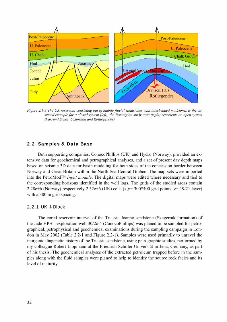
The second 3D block under study is located somewhere in the east of the British study area in the Norwegian sector. This area contains a variety of reservoirs, from Oxfordian to Cre-taceous age. The Late Jurassic Oxfordian Sands of the Fulmar Formation are encountered in similar settings as the British Triassic formations described above. These sands have an aver-age thickness of about 80 m are encountered in the Norwegian study area. Top of the structure is at -4240 m TVDSS. The field was discovered in the early seventies, and developed since. The sand unit drapes over a Jurassic/Triassic rotated horst block and represents a four-way clo-sure. Source rocks in the area are the shales of the

• Mandal Formation, the Norwegian equivalent of the Kimmeridge Clay (Figure 4.1-7),

• Farsund Formations (Heather)

• and Bryne (Pentland) Formations,

the latter two being present at the top of the structure, the first one missing at the struc-ture (Figure 2.1-3).

31

RotliegendesOxfordian

Gas Cap

Dry (res. HC)

Post-Paleocene

U. Paleocene

Hod

U. Chalk Group

Farsund Sands

Post-Paleocene

U. Paleocene

U. Chalk

Joanne

Julius

JudySmithbank

Hod Jurassic

RotliegendesOxfordian

Gas Cap

Dry (res. HC)

Post-Paleocene

U. Paleocene

Hod

U. Chalk Group

Farsund Sands

RotliegendesOxfordian

Gas Cap

Dry (res. HC)

Post-Paleocene

U. Paleocene

Hod

U. Chalk Group

Farsund Sands

Post-Paleocene

U. Paleocene

U. Chalk

Joanne

Julius

JudySmithbank

Hod Jurassic

Post-Paleocene

U. Paleocene

U. Chalk

Joanne

Julius

JudySmithbank

Hod

Post-Paleocene

U. Paleocene

U. Chalk

Joanne

Julius

JudySmithbank

Hod Jurassic

Figure 2.1-3 The UK reservoir, consisting out of mainly fluvial sandstones with interbedded mudstones is the as-sumed example for a closed system (left), the Norwegian study area (right) represents an open system (Farsund Sands, Oxfordian and Rotliegendes).

2.2 Samples & Data Base

Both supporting companies, ConocoPhillips (UK) and Hydro (Norway), provided an ex-tensive data for geochemical and petrographical analyses, and a set of present day depth maps based on seismic 3D data for basin modeling for both sides of the concession border between Norway and Great Britain within the North Sea Central Graben. The map sets were imported into the PetroMod™ Input module. The digital maps were edited where necessary and tied to the corresponding horizons identified in the well logs. The grids of the studied areas contain 2.28e+6 (Norway) respectively 2.52e+6 (UK) cells (x,y= 300*400 grid points; z= 19/21 layer) with a 300 m grid spacing.

2.2.1 UK J-Block

The cored reservoir interval of the Triassic Joanne sandstone (Skagerrak formation) of the Jade HPHT exploration well 30/2c-4 (ConocoPhillips) was planed to be sampled for petro-graphical, petrophysical and geochemical examinations during the sampling campaign in Lon-don in May 2002 (Table 2.2-1 and Figure 2.2-1). Samples were used primarily to unravel the inorganic diagenetic history of the Triassic sandstone, using petrographic studies, performed by my colleague Robert Lippmann at the Friedrich Schiller Universiät in Jena, Germany, as part of his thesis. The geochemical analyses of the extracted petroleum trapped before in the sam-ples along with the fluid samples were planed to help to identify the source rock facies and its level of maturity.

32

Table 2.2-1 Sample set from Jade well 30/2c-4 (UK) for geochemical and petrographical analyses.

GFZ-No. Depth (m TVDSS) Lithology Period/Age Formation/Member

G000123 4750.0 siltst-sst Triassic/Carnian Skagerrak /JoanneG000124 4752.7 siltst-sst Triassic/Carnian Skagerrak /Joanne

sst Triassic/Carnian Skagerrak /JoanneG000125 4754.2 sst Triassic/Carnian Skagerrak /JoanneG000126 4757.3 sst Triassic/Carnian Skagerrak /JoanneG000127 4758.8 sst Triassic/Carnian Skagerrak /JoanneG000128 4759.2 sst Triassic/Carnian Skagerrak /JoanneG000129 4762.3 siltst-sst Triassic/Carnian Skagerrak /JoanneG000130 4763.4 siltst-sst Triassic/Carnian Skagerrak /JoanneG000131 4764.5 sst Triassic/Carnian Skagerrak /JoanneG000132 4765.4 siltst-sst Triassic/Carnian Skagerrak /JoanneG000133 4766.7 sst Triassic/Carnian Skagerrak /JoanneG000134 4768.6 sst Triassic/Carnian Skagerrak /JoanneG000135 4769.0 sst Triassic/Carnian Skagerrak /JoanneG000136 4771.5 sst Triassic/Carnian Skagerrak /JoanneG000137 4771.8 sst Triassic/Carnian Skagerrak /JoanneG000138 4773.1 sst/siltst Triassic/Carnian Skagerrak /JoanneG000139 4776.7 sst Triassic/Carnian Skagerrak /JoanneG000140 4778.0 sst Triassic/Carnian Skagerrak /JoanneG000141 4779.3 sst Triassic/Carnian Skagerrak /JoanneG000142 4780.8 sst Triassic/Carnian Skagerrak /JoanneG000143 4781.8 sst Triassic/Carnian Skagerrak /JoanneG000144 4782.3 sst Triassic/Carnian Skagerrak /JoanneG000145 4782.5 sst Triassic/Carnian Skagerrak /JoanneG000146 4786.6 sst Triassic/Carnian Skagerrak /JoanneG000147 4789.8 sst Triassic/Carnian Skagerrak /JoanneG000148 4790.2 sst Triassic/Carnian Skagerrak /JoanneG000149 4791.0 sh-siltst Triassic/Carnian Skagerrak /JoanneG000150 4792.2 sst Triassic/Carnian Skagerrak /JoanneG000151 4797.2 sst Triassic/Carnian Skagerrak /JoanneG000152 4798.0 sst Triassic/Carnian Skagerrak /JoanneG000153 4798.5 sst Triassic/Carnian Skagerrak /JoanneG000154 4799.1 sst Triassic/Carnian Skagerrak /JoanneG000155 4800.6

Skagerrak /JoanneG000156 4800.9 sh Triassic/Carniansst Triassic/Carnian Skagerrak /JoanneG000157 4800.3

Skagerrak /JoanneG000158 4802.7 sh Triassic/CarnianSkagerrak /JoanneG000159 4806.3 sh Triassic/Carnian

sst Triassic/Carnian Skagerrak /JoanneG000160 4813.6 G000363 4710 DST 1 Triassic/Carnian Skagerrak /Joanne

G000364 4889 DST 2 Triassic/Carnian Skagerrak /Joanne

33

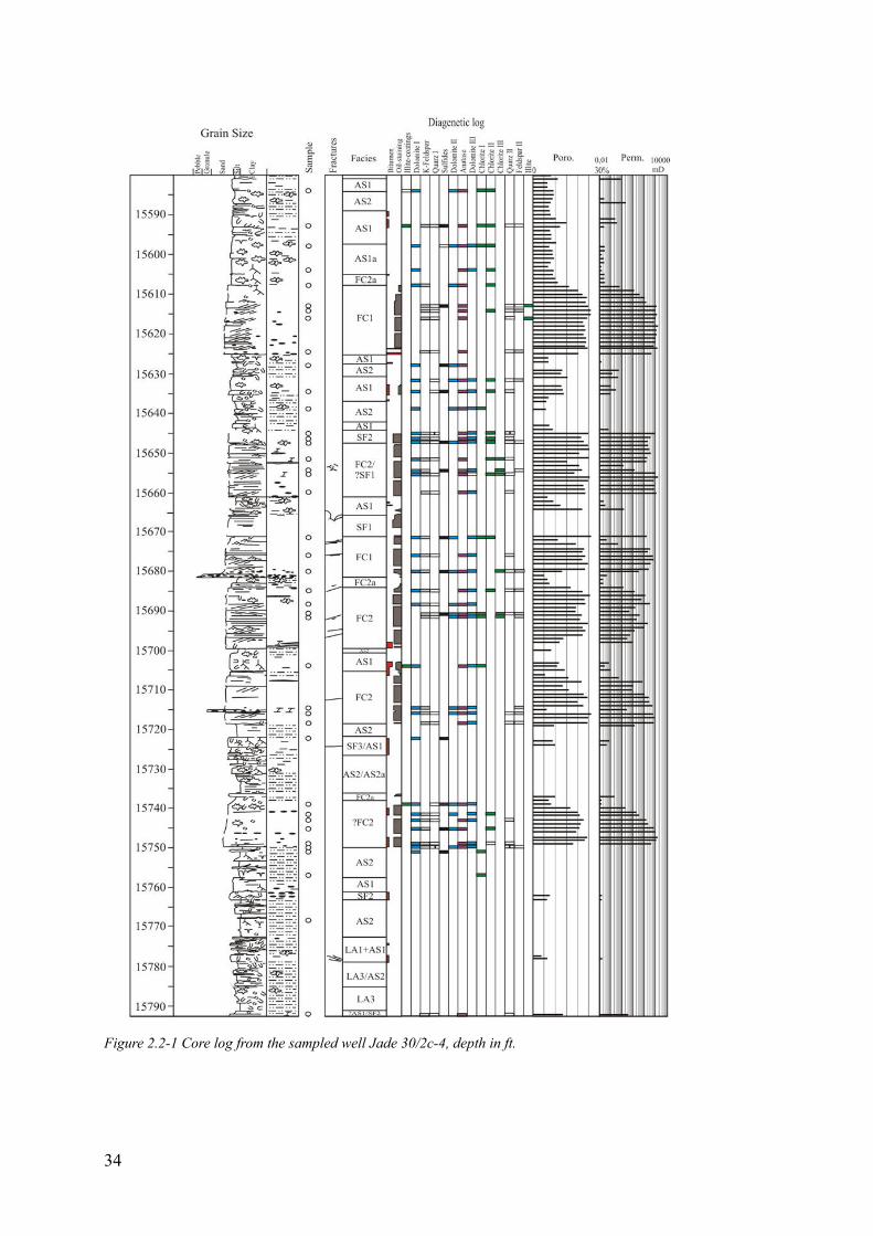
Figure 2.2-1 Core log from the sampled well Jade 30/2c-4, depth in ft.

34

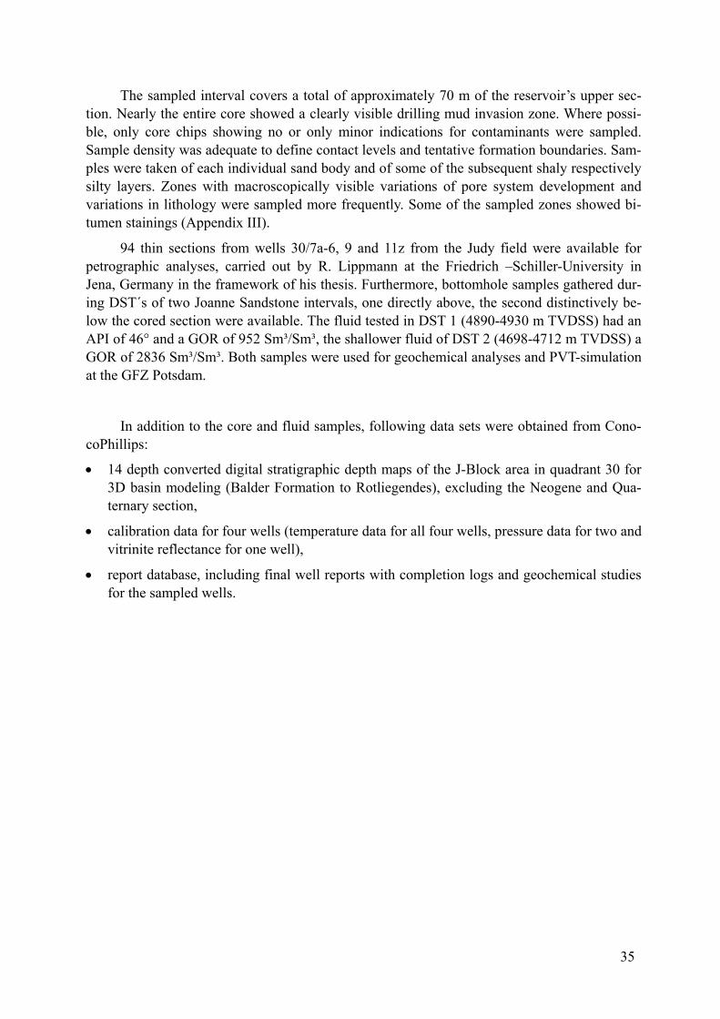
The sampled interval covers a total of approximately 70 m of the reservoir’s upper sec-tion. Nearly the entire core showed a clearly visible drilling mud invasion zone. Where possi-ble, only core chips showing no or only minor indications for contaminants were sampled. Sample density was adequate to define contact levels and tentative formation boundaries. Sam-ples were taken of each individual sand body and of some of the subsequent shaly respectively silty layers. Zones with macroscopically visible variations of pore system development and variations in lithology were sampled more frequently. Some of the sampled zones showed bi-tumen stainings (Appendix III).

94 thin sections from wells 30/7a-6, 9 and 11z from the Judy field were available for petrographic analyses, carried out by R. Lippmann at the Friedrich –Schiller-University in Jena, Germany in the framework of his thesis. Furthermore, bottomhole samples gathered dur-ing DST´s of two Joanne Sandstone intervals, one directly above, the second distinctively be-low the cored section were available. The fluid tested in DST 1 (4890-4930 m TVDSS) had an API of 46° and a GOR of 952 Sm³/Sm³, the shallower fluid of DST 2 (4698-4712 m TVDSS) a GOR of 2836 Sm³/Sm³. Both samples were used for geochemical analyses and PVT-simulation at the GFZ Potsdam.

In addition to the core and fluid samples, following data sets were obtained from Cono-coPhillips:

• 14 depth converted digital stratigraphic depth maps of the J-Block area in quadrant 30 for 3D basin modeling (Balder Formation to Rotliegendes), excluding the Neogene and Qua-ternary section,

• calibration data for four wells (temperature data for all four wells, pressure data for two and vitrinite reflectance for one well),

• report database, including final well reports with completion logs and geochemical studies for the sampled wells.

35

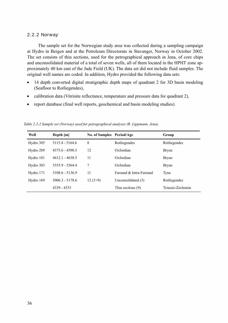
2.2.2 Norway

The sample set for the Norwegian study area was collected during a sampling campaign at Hydro in Bergen and at the Petroleum Directorate in Stavanger, Norway in October 2002. The set consists of thin sections, used for the petrographical approach in Jena, of core chips and unconsolidated material of a total of seven wells, all of them located in the HPHT zone ap-proximately 40 km east of the Jade Field (UK). The data set did not include fluid samples. The original well names are coded. In addition, Hydro provided the following data sets:

• 14 depth converted digital stratigraphic depth maps of quadrant 2 for 3D basin modeling (Seafloor to Rotliegendes),

• calibration data (Vitrinite reflectance, temperature and pressure data for quadrant 2),

• report database (final well reports, geochemical and basin modeling studies).

Table 2.2-2 Sample set (Norway) used for petrographical analyses (R. Lippmann, Jena).

Well Depth [m] No. of Samples Period/Age Group

Hydro 305 5115.4 - 5164.6 8 Rotliegendes Rotliegendes

Hydro 289 4575.6 - 4590.5 12 Oxfordian Bryne

Hydro 181 4612.1 - 4638.5 11 Oxfordian Bryne

Hydro 303 5555.9 - 5564.4 7 Oxfordian Bryne

Hydro 171 5108.6 - 5136.9 11 Farsund & Intra-Farsund Tyne

Hydro 169 5006.3 - 5178.6 12 (3+9) Unconsolidated (3) Rotliegendes

4339 - 4353 Thin sections (9) Triassic/Zechstein

36

3 Organic Geochemistry

Organic geochemistry was employed to gather important compositional information on fluids and reservoir cores, prior to embarking on the main task of modeling overpressure gen-eration.

3.1 Methods

Solvent extracts of 30 core samples and two gas condensates from the British Jade well 30/2c-4 were separated into compound classes by means of medium-pressure liquid chroma-tography (MPLC), analyzed by gas chromatography (GC) and gas chromatography – mass spectrometry (GCMS) and interpreted using the software package Chemstation, Rev. A 08.03.

3.1.1 Soxhlet-extraction, MPLC

First, the chunks of the sampled core were crushed manually to pieces having an average weight of ~ 20 g each. Then, the pieces where submitted into a Soxhlet apparatus, and continu-ously extracted and heated for 24 h, using a 99:1 dichloromethane-methanol mixture as solvent for the extractable organic matter. The extract was concentrated to 1 ml for each sample using a Turbovap apparatus. Its hexane-soluble portion was separated by MPLC into fractions of ali-phatic hydrocarbons, aromatic hydrocarbons, and polar compounds (NSO fraction). Andro-stane (c 5.0 mg/ml) and Ethylpyrene (c 2.5 mg/ml) were added as internal standards.

3.1.2 GC-MS

Aliphatic and aromatic hydrocarbons were analyzed by GC-MS, carried out on an Agilent 6890 GC interfaced with a Finnigan MAT95XL mass spectrometer for peak identifica-tion. The GC was equipped with a Agilent Ultra 1 Methyl Siloxane column with a length of 50 m, an inner diameter of 0.2 mm, and a film thickness of 0,33 µm. Chosen operation mode was constant flow with a helium flow rate of 1.0 ml/min and a temperature program from 40-300°C (40°C, 2 min hold time, then to 300°C with a heating rate of 5°C/min). The programmable temperature vaporizing inlet operated in a splitless mode from 40°C in steps of 7°C/min. to 300°C for 3 minutes.

In addition to the analyzed data from this study, reported data from the Judy Field South of the Jade structure were included (originally reported in Swarbrick et al., 2000), as well as data from (Hughes et al., 1985), who investigated a variety of Central Graben oils, mainly from Cretaceous plays.

No source rock material, either for the UK or for the Norwegian study area was accessi-ble for investigations. In addition, only samples from the upper section of the reservoir of the Jade well were available, since the cored interval of the UK well 30/2c-4 does not penetrate the entire reservoir section.

In the following, the oil compositional information as provided by ConocoPhillips is de-scribed and compared to the analytical results of both, the two gas condensates tested in the

37

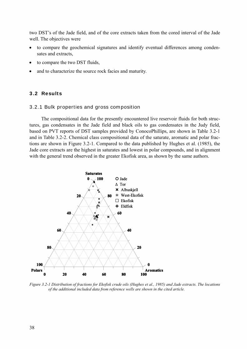
two DST’s of the Jade field, and of the core extracts taken from the cored interval of the Jade well. The objectives were

• to compare the geochemical signatures and identify eventual differences among conden-sates and extracts,

• to compare the two DST fluids,

• and to characterize the source rock facies and maturity.

3.2 Results

3.2.1 Bulk properties and gross composition

The compositional data for the presently encountered live reservoir fluids for both struc-tures, gas condensates in the Jade field and black oils to gas condensates in the Judy field, based on PVT reports of DST samples provided by ConocoPhillips, are shown in Table 3.2-1 and in Table 3.2-2. Chemical class compositional data of the saturate, aromatic and polar frac-tions are shown in Figure 3.2-1. Compared to the data published by Hughes et al. (1985), the Jade core extracts are the highest in saturates and lowest in polar compounds, and in alignment with the general trend observed in the greater Ekofisk area, as shown by the same authors.

0 20 40 60 80 100

100

80

60

40

20

0100

80

60

40

20

0

Aromatics

Saturates

Polars

Jade∆ Tor

AlbuskjellWest-EkofiskEkofiskEldfisk

0 20 40 60 80 100

100

80

60

40

20

0100

80

60

40

20

0

Aromatics

Saturates

Polars0 20 40 60 80 100

100

80

60

40

20

0100

80

60

40

20

0

Aromatics

Saturates

Polars

Jade∆ Tor

AlbuskjellWest-EkofiskEkofiskEldfisk

Figure 3.2-1 Distribution of fractions for Ekofisk crude oils (Hughes et al., 1985) and Jade extracts. The locations of the additional included data from reference wells are shown in the cited article.

38

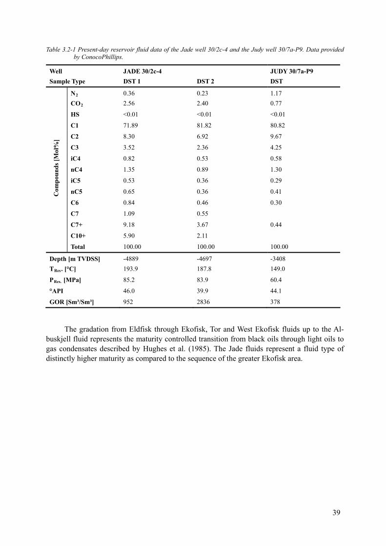
Table 3.2-1 Present-day reservoir fluid data of the Jade well 30/2c-4 and the Judy well 30/7a-P9. Data provided by ConocoPhillips.

Well JADE 30/2c-4 JUDY 30/7a-P9 Sample Type DST 1 DST 2 DST

N 0.36 0.23 1.17 2

CO 2.56 2.40 0.77 2

HS <0.01 <0.01 <0.01

C1 71.89 81.82 80.82

C2 8.30 6.92 9.67

Com

poun

ds [M

ol%

]

C3 3.52 2.36 4.25

iC4 0.82 0.53 0.58

nC4 1.35 0.89 1.30

iC5 0.53 0.36 0.29

nC5 0.65 0.36 0.41

C6 0.84 0.46 0.30

C7 1.09 0.55

C7+ 9.18 3.67 0.44

C10+ 5.90 2.11

Total 100.00 100.00 100.00

Depth [m TVDSS] -4889 -4697 -3408 T . [°C] 193.9 187.8 149.0 Res

P [MPa] 85.2 83.9 60.4 Res.

°API 46.0 39.9 44.1

GOR [Sm³/Sm³] 952 2836 378

The gradation from Eldfisk through Ekofisk, Tor and West Ekofisk fluids up to the Al-buskjell fluid represents the maturity controlled transition from black oils through light oils to gas condensates described by Hughes et al. (1985). The Jade fluids represent a fluid type of distinctly higher maturity as compared to the sequence of the greater Ekofisk area.

39

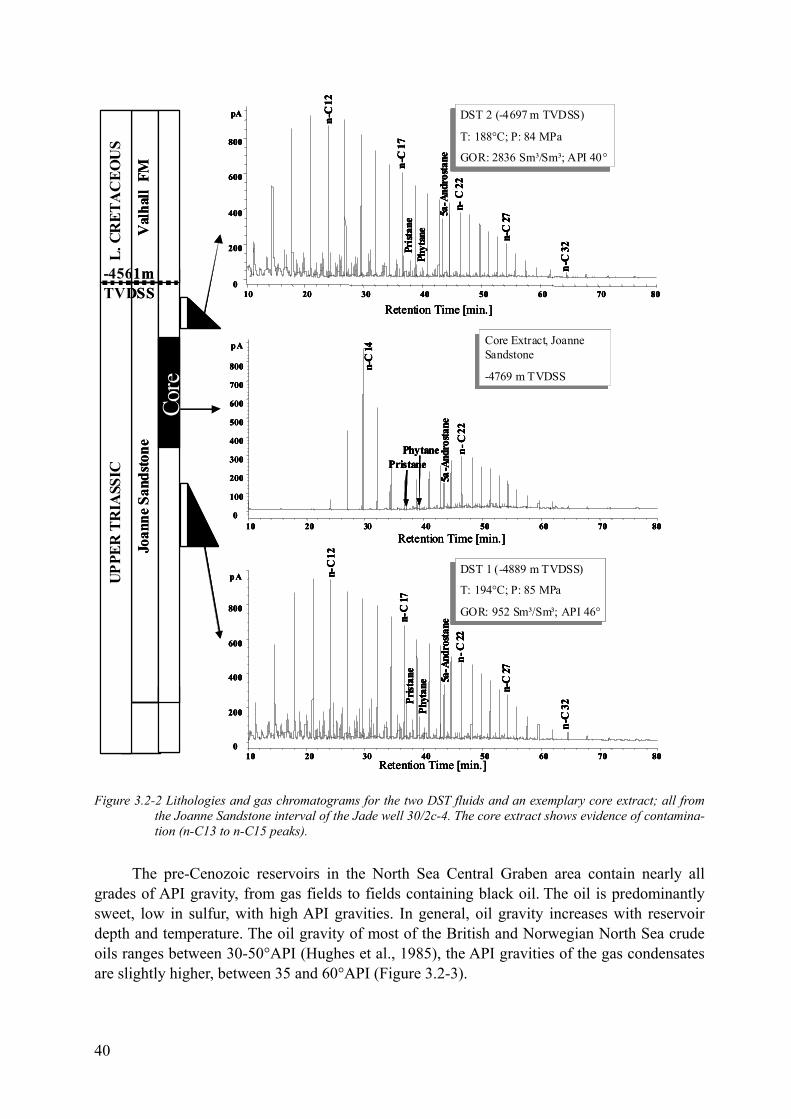
Joan

ne S

ands

tone

Val

hall

FM

UPPE

R T

RIA

SSIC

L. C

RET

AC

EOU

S

Core

-4561m TVDSS 8010 20 30 40 50 60 70

pA

0

200

400

600

800

n-C

12

Prist

ane

Phyt

ane

5a-A

ndro

stane

n-C

22

Retention Time [min.]

DST 2 (-4697 m TVDSS)

T: 188°C; P: 84 MPa

GOR: 2836 Sm³/Sm³; API 40°

DST 2 (-4697 m TVDSS)

T: 188°C; P: 84 MPa

GOR: 2836 Sm³/Sm³; API 40°

n-C

17

n-C

32n-

C 27

8010 20 30 40 50 60 70

pA

0

200

400

600

800

n-C

12

Prist

ane

Phyt

ane

5a-A

ndro

stane

n-C

22

Retention Time [min.]

DST 2 (-4697 m TVDSS)

T: 188°C; P: 84 MPa

GOR: 2836 Sm³/Sm³; API 40°

DST 2 (-4697 m TVDSS)

T: 188°C; P: 84 MPa

GOR: 2836 Sm³/Sm³; API 40°

n-C

17

n-C

32n-

C 27

8010 20 30 40 50 60 70

pA

0

200

400

600

800

n-C

27

Prist

ane

Phyt

ane 5a

-And

rosta

nen-

C 22

Retention Time [min.]

DST 1 (-4889 m TVDSS)

T: 194°C; P: 85 MPa

GOR: 952 Sm³/Sm³; API 46°

DST 1 (-4889 m TVDSS)

T: 194°C; P: 85 MPa

GOR: 952 Sm³/Sm³; API 46°

n-C

12

n-C

17

n-C

32

8010 20 30 40 50 60 70

pA

0

200

400

600

800

n-C

27

Prist

ane

Phyt

ane 5a

-And

rosta

nen-

C 22

Retention Time [min.]

DST 1 (-4889 m TVDSS)

T: 194°C; P: 85 MPa

GOR: 952 Sm³/Sm³; API 46°

DST 1 (-4889 m TVDSS)

T: 194°C; P: 85 MPa

GOR: 952 Sm³/Sm³; API 46°

n-C

12

n-C

17

n-C

32

8010 20 30 40 50 60 70

pA

0

100

200

300

400

500

600

700

800 n-C

14

PristanePhytane

5a-A

ndro

stane

n-C

22

Retention Time [min.]

Core Extract, Joanne Sandstone

-4769 m TVDSS

Core Extract, Joanne Sandstone

-4769 m TVDSS

8010 20 30 40 50 60 70

pA

0

100

200

300

400

500

600

700

800 n-C

14

PristanePhytane

5a-A

ndro

stane

n-C

22

Retention Time [min.]

Core Extract, Joanne Sandstone

-4769 m TVDSS

Core Extract, Joanne Sandstone

-4769 m TVDSS

Joan

ne S

ands

tone

Val

hall

FM

UPPE

R T

RIA

SSIC

L. C

RET

AC

EOU

S

Core

-4561m TVDSS 8010 20 30 40 50 60 70

pA

0

200

400

600

800

n-C

12

Prist

ane

Phyt

ane

5a-A

ndro

stane

n-C

22

Retention Time [min.]

DST 2 (-4697 m TVDSS)

T: 188°C; P: 84 MPa

GOR: 2836 Sm³/Sm³; API 40°

DST 2 (-4697 m TVDSS)

T: 188°C; P: 84 MPa

GOR: 2836 Sm³/Sm³; API 40°

n-C

17

n-C

32n-

C 27

8010 20 30 40 50 60 70

pA

0

200

400

600

800

n-C

12

Prist

ane

Phyt

ane

5a-A

ndro

stane

n-C

22

Retention Time [min.]

DST 2 (-4697 m TVDSS)

T: 188°C; P: 84 MPa

GOR: 2836 Sm³/Sm³; API 40°

DST 2 (-4697 m TVDSS)

T: 188°C; P: 84 MPa

GOR: 2836 Sm³/Sm³; API 40°

n-C

17

n-C

32n-

C 27

8010 20 30 40 50 60 70

pA

0

200

400

600

800

n-C

27

Prist

ane

Phyt

ane 5a

-And

rosta

nen-

C 22

Retention Time [min.]

DST 1 (-4889 m TVDSS)

T: 194°C; P: 85 MPa

GOR: 952 Sm³/Sm³; API 46°

DST 1 (-4889 m TVDSS)

T: 194°C; P: 85 MPa

GOR: 952 Sm³/Sm³; API 46°

n-C

12

n-C

17

n-C

32

8010 20 30 40 50 60 70

pA

0

200

400

600

800

n-C

27

Prist

ane

Phyt

ane 5a

-And

rosta

nen-

C 22

Retention Time [min.]

DST 1 (-4889 m TVDSS)

T: 194°C; P: 85 MPa

GOR: 952 Sm³/Sm³; API 46°

DST 1 (-4889 m TVDSS)

T: 194°C; P: 85 MPa

GOR: 952 Sm³/Sm³; API 46°

n-C

12

n-C

17

n-C

32

8010 20 30 40 50 60 70

pA

0

100

200

300

400

500

600

700

800 n-C

14

PristanePhytane

5a-A

ndro

stane

n-C

22

Retention Time [min.]

Core Extract, Joanne Sandstone

-4769 m TVDSS

Core Extract, Joanne Sandstone

-4769 m TVDSS

8010 20 30 40 50 60 70

pA

0

100

200

300

400

500

600

700

800 n-C

14

PristanePhytane

5a-A

ndro

stane

n-C

22

Retention Time [min.]

Core Extract, Joanne Sandstone

-4769 m TVDSS

Core Extract, Joanne Sandstone

-4769 m TVDSS

Figure 3.2-2 Lithologies and gas chromatograms for the two DST fluids and an exemplary core extract; all from the Joanne Sandstone interval of the Jade well 30/2c-4. The core extract shows evidence of contamina-tion (n-C13 to n-C15 peaks).

The pre-Cenozoic reservoirs in the North Sea Central Graben area contain nearly all grades of API gravity, from gas fields to fields containing black oil. The oil is predominantly sweet, low in sulfur, with high API gravities. In general, oil gravity increases with reservoir depth and temperature. The oil gravity of most of the British and Norwegian North Sea crude oils ranges between 30-50°API (Hughes et al., 1985), the API gravities of the gas condensates are slightly higher, between 35 and 60°API (Figure 3.2-3).

40

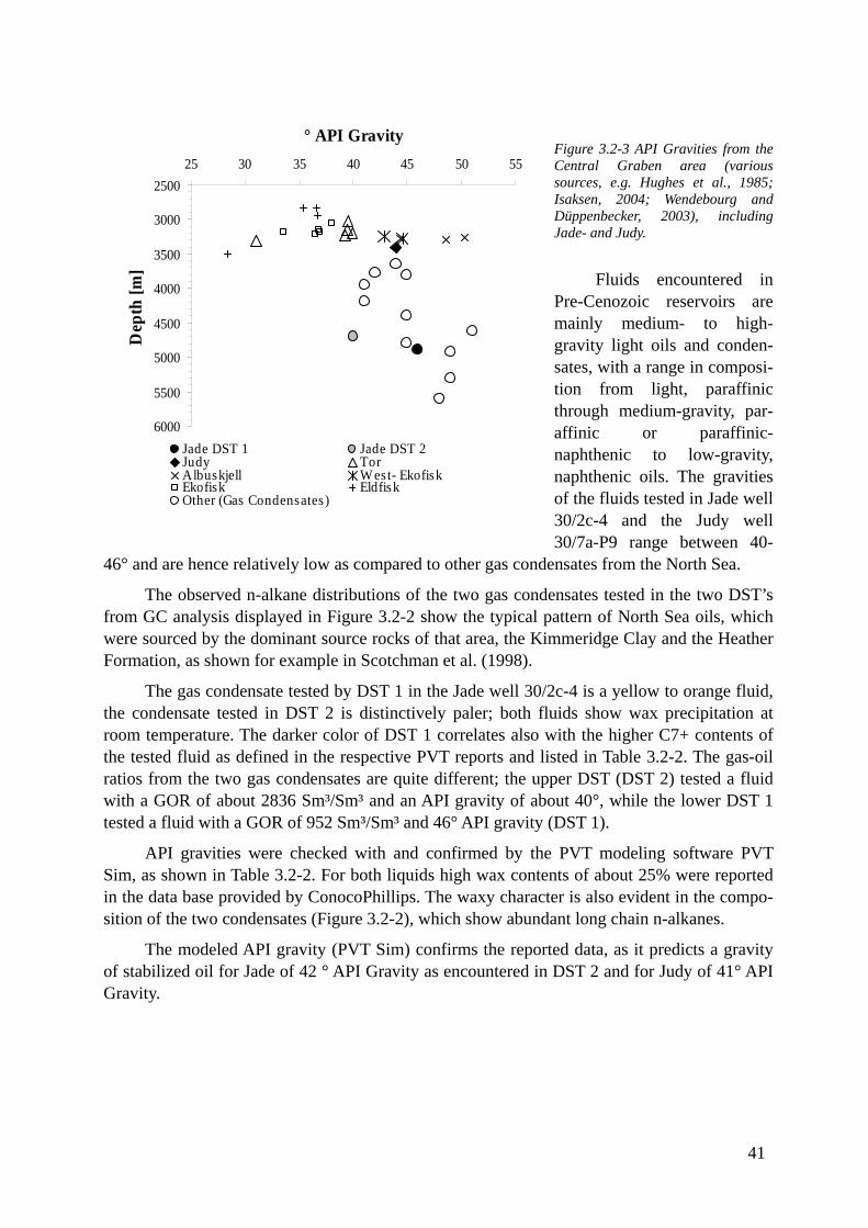
41

Figure 3.2-3 API Gravities from the Central Graben area (various sources, e.g. Hughes et al., 1985; Isaksen, 2004; Wendebourg and Düppenbecker, 2003), including Jade- and Judy.

Fluids encountered in Pre-Cenozoic reservoirs are mainly medium- to high-gravity light oils and conden-sates, with a range in composi-tion from light, paraffinic through medium-gravity, par-affinic or paraffinic-naphthenic to low-gravity, naphthenic oils. The gravities of the fluids tested in Jade well 30/2c-4 and the Judy well 30/7a-P9 range between 40-

46° and are hence relatively low as compared to other gas condensates from the North Sea.

The observed n-alkane distributions of the two gas condensates tested in the two DST’s from GC analysis displayed in Figure 3.2-2 show the typical pattern of North Sea oils, which were sourced by the dominant source rocks of that area, the Kimmeridge Clay and the Heather Formation, as shown for example in Scotchman et al. (1998).

The gas condensate tested by DST 1 in the Jade well 30/2c-4 is a yellow to orange fluid, the condensate tested in DST 2 is distinctively paler; both fluids show wax precipitation at room temperature. The darker color of DST 1 correlates also with the higher C7+ contents of the tested fluid as defined in the respective PVT reports and listed in Table 3.2-2. The gas-oil ratios from the two gas condensates are quite different; the upper DST (DST 2) tested a fluid with a GOR of about 2836 Sm³/Sm³ and an API gravity of about 40°, while the lower DST 1 tested a fluid with a GOR of 952 Sm³/Sm³ and 46° API gravity (DST 1).

API gravities were checked with and confirmed by the PVT modeling software PVT Sim, as shown in Table 3.2-2. For both liquids high wax contents of about 25% were reported in the data base provided by ConocoPhillips. The waxy character is also evident in the compo-sition of the two condensates (Figure 3.2-2), which show abundant long chain n-alkanes.

The modeled API gravity (PVT Sim) confirms the reported data, as it predicts a gravity of stabilized oil for Jade of 42 ° API Gravity as encountered in DST 2 and for Judy of 41° API Gravity.

2500

3000

3500

4000

4500

5000

5500

6000

25 30 35 40 45 50 55

° API GravityD

epth

[m]

Jade DST 1 Jade DST 2Judy TorAlbuskjell West- EkofiskEkofisk EldfiskOther (Gas Condensates)

Table 3.2-2 Phase and fluid properties of the fluid tested in DST 1 of the Jade well 30/2c-4. Input data was pro-vided by ConocoPhillips.

30/2c-4 DST 1 EOS: SRK Peneloux Gravity of stabilized oil: 42.46°API

Phase Properties: @ 446 bar and 194°C @ 1 bar and 15°C (flashed to surface)

Total Vapor Liquid Total Vapor Liquid

Mole [%] 100.00 100.00 0.00 100.00 90.37 9.63 Weight [%] 100.00 100.00 0.00 100.00 51.68 48.32 Volume [cm³/mol] 104.63 104.63 121.47 21312.59 23559.74 232.03Volume [%] 100.00 100.00 0.00 100.00 99.90 0.10 Density 0.3596 0.3596 0.5124 0.0018 0.0009 0.8134Z Factor 1.2021 1.2021 1.3956 0.9013 0.9964 0.0098Molecular Weight 37.62 37.62 62.25 37.62 21.52 188.72

Total Vapor Liquid Total Vapor Liquid Extended Fluid Properties: [mole%] [mole%] [mole%] [mole%] [mole%] [mole%]

N2 0.360 0.360 0.286 0.360 0.398 0.001 CO2 2.560 2.560 2.397 2.560 2.828 0.047 H2S 0.010 0.010 0.011 0.010 0.011 0.001 C1 71.883 71.883 63.236 71.883 79.500 0.424 C2 8.299 8.299 8.118 8.299 9.148 0.334 C3 3.520 3.520 3.680 3.520 3.835 0.557 iC4 0.820 0.820 0.892 0.820 0.872 0.327 nC4 1.350 1.350 1.509 1.350 1.409 0.796 iC5 0.530 0.530 0.618 0.530 0.503 0.780 nC5 0.650 0.650 0.769 0.650 0.586 1.251 C6 0.840 0.840 1.044 0.840 0.514 3.895 C7 1.090 1.090 1.459 1.090 0.234 9.116 C8 1.240 1.240 1.725 1.240 0.118 11.762C9 0.950 0.950 1.373 0.950 0.031 9.569 C10-C11 1.257 1.257 1.900 1.257 0.010 12.962C12-C13 0.989 0.989 1.589 0.989 0.001 10.262C14-C15 0.779 0.779 1.340 0.779 0.000 8.082 C16-C18 0.868 0.868 1.648 0.868 0.000 9.012 C19-C20 0.428 0.428 0.893 0.428 0.000 4.440 C21-C24 0.601 0.601 1.430 0.601 0.000 6.243 C25-C28 0.372 0.372 1.069 0.372 0.000 3.866 C29-C35 0.344 0.344 1.284 0.344 0.000 3.569 C36-C80 0.261 0.261 1.732 0.261 0.000 2.705 Total 100 100 100 100 100 100

42

3.2.2 Contamination

As described in section 2.5, nearly the entire core showed a clearly visible drilling mud invasion zone. Although only core chips showing no or only minor indications for contami-nants were sampled, GC-MS analysis of the core extracts indicated the presence of a contami-nation in the core samples studied. Figure 3.2-2 shows the distinct characteristics of the ali-phatic hydrocarbons from GC analyses for the two DST’s (uncontaminated) and one example for the core extracts (contaminated). Based on the distribution of aliphatic hydrocarbons, the prominent peaks between n-C12 and n-C16, which were observed in all core extracts, suggest a high concentration of contaminant (drilling mud additive). This suggestion is supported by the outer appearance of the cores, as seen at the sample campaign in May 2002 in London, and the reported contamination in the database provided by ConocoPhillips (LGC-Geochemistry, 1997). Despite the contamination, the ratios from the resolved compounds such as the ratio of the isoprenoids pristane and phytane are most likely unaffected.

3.2.3 Facies and maturity

3.2.3.1 Isoprenoids

Both, pristane and phytane, are degradation products of phytol, the latter being a compo-nent of chlorophyll a. Pristane is the product of diagenetic conversion under oxic depositional conditions, and phytane under reducing conditions. Brooks et al.(1969) and later Powell et al.(1988) proposed the pristane/phytane (Pr/Ph) ratio as an indicator of the redox conditions of the depositional environment. Although phytane can come from sources other than phytol (ten Haven et al., 1987), Pr/Ph is widely used as a geogenic environmental indicator. Didyk et al. (1978) suggested that Pr/Ph ratios substantially below 1.0 indicate anoxic, highly reducing de-positional environments, and Pr/Ph ratios above 1.0 indicate oxic environments. North Sea crude oils which originated from the type II kerogen of the Kimmeridge Clay Formation ex-hibit Pr/Ph ratios of 1.0 to 1.5, while oils originated from the mixed source of the Heather Formation (marine shale with terrestrial input) show Pr/Ph ratios well above 1.5 (Kubala et al., 2003).

Isoprenoid and n-alkane data provide valuable information on biodegradation, maturity and diagenetic conditions. With increasing maturity, n-alkanes are generated faster than isopre-noids, resulting in a decrease in isoprenoid/n-alkane ratios. Biodegradation, in contrast, re-moves n-alkanes and increases thereby the isoprenoid/alkane ratios.

All analyzed samples from the Jade well 30/2c-4 show similar, depth independent Pr/Ph ratios in the range of 1.0 to 1.8.; they are in concordance with the general trend reported by Hughes et al. (1985), as shown in Figure 3.2-4, and indicate an oxic depositional environment of the source rock. The pristane to n-heptadecane versus phytane to n-octadecane ratios dis-played in Figure 3.2-4 show a fairly narrow range for all ratios of core extracts and gas con-densates of the Jade field; the ratios are in alignment with the general trend observed in the Central Graben area as reported by Hughes et al. (1985), who investigated the geochemical signatures of crude oils from mainly Cretaceous reservoirs of the greater Norwegian Ekofisk

43

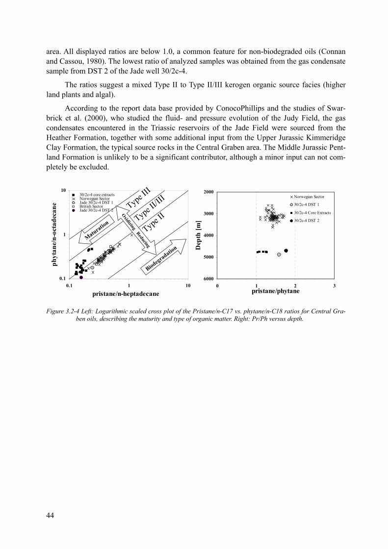
area. All displayed ratios are below 1.0, a common feature for non-biodegraded oils (Connan and Cassou, 1980). The lowest ratio of analyzed samples was obtained from the gas condensate sample from DST 2 of the Jade well 30/2c-4.

The ratios suggest a mixed Type II to Type II/III kerogen organic source facies (higher land plants and algal).

According to the report data base provided by ConocoPhillips and the studies of Swar-brick et al. (2000), who studied the fluid- and pressure evolution of the Judy Field, the gas condensates encountered in the Triassic reservoirs of the Jade Field were sourced from the Heather Formation, together with some additional input from the Upper Jurassic Kimmeridge Clay Formation, the typical source rocks in the Central Graben area. The Middle Jurassic Pent-land Formation is unlikely to be a significant contributor, although a minor input can not com-pletely be excluded.

2000

3000

4000

5000

60000 1 2

pristane/phytane

Dep

th [m

]

3

Norwegian Sector

30/2c-4 DST 1

30/2c-4 Core Extracts

30/2c-4 DST 2

0.1

1

10

0.1 1 10

pristane/n-heptadecane

phyt

ane/

n-oc

tade

cane

30/2c-4 core extractsNorwegian SectorJade 30/2c-4 DST 1British SectorJade 30/2c-4 DST 2 Type I

II

Type II/III

Type II

Maturation

Biodegradation

Oxidizing Reducing

2000

3000

4000

5000

60000 1 2

pristane/phytane

Dep

th [m

]

3

Norwegian Sector

30/2c-4 DST 1

30/2c-4 Core Extracts

30/2c-4 DST 2

0.1

1

10

0.1 1 10

pristane/n-heptadecane

phyt

ane/

n-oc

tade

cane

30/2c-4 core extractsNorwegian SectorJade 30/2c-4 DST 1British SectorJade 30/2c-4 DST 2 Type I

II

Type II/III

Type II

Maturation

Biodegradation

Oxidizing Reducing

Figure 3.2-4 Left: Logarithmic scaled cross plot of the Pristane/n-C17 vs. phytane/n-C18 ratios for Central Gra-

ben oils, describing the maturity and type of organic matter. Right: Pr/Ph versus depth.

44

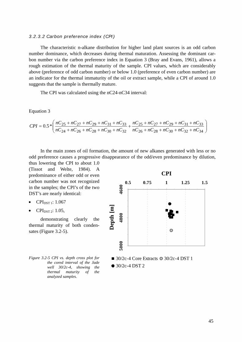
45

4600

4800

5000

0.5 0.75 1 1.25 1.5

CPI

Dep

th [m

]

30/2c-4 Core Extracts 30/2c-4 DST 130/2c-4 DST 2

3.2.3.2 Carbon preference index (CPI)

The characteristic n-alkane distribution for higher land plant sources is an odd carbon number dominance, which decreases during thermal maturation. Assessing the dominant car-bon number via the carbon preference index in Equation 3 (Bray and Evans, 1961), allows a rough estimation of the thermal maturity of the sample. CPI values, which are considerably above (preference of odd carbon number) or below 1.0 (preference of even carbon number) are an indicator for the thermal immaturity of the oil or extract sample, while a CPI of around 1.0 suggests that the sample is thermally mature.

The CPI was calculated using the nC24-nC34 interval:

Equation 3

⎟⎟⎠

⎞⎜⎜⎝

⎛++++++++

+++++++++

=3432302826

3331292725

3230282624

3331292725*5.0nCnCnCnCnCnCnCnCnCnC

nCnCnCnCnCnCnCnCnCnC

CPI

In the main zones of oil formation, the amount of new alkanes generated with less or no odd preference causes a progressive disappearance of the odd/even predominance by dilution, thus lowering the CPI to about 1.0 (Tissot and Welte, 1984). A predominance of either odd or even carbon number was not recognized in the samples; the CPI’s of the two DST’s are nearly identical:

• CPIDST 1: 1.067

• CPIDST 2: 1.05,

demonstrating clearly the thermal maturity of both conden-sates (Figure 3.2-5).

Figure 3.2-5 CPI vs. depth cross plot for the cored interval of the Jade well 30/2c-4, showing the thermal maturity of the analyzed samples.

3.2.3.3 Biomarkers

All samples were analyzed with respect to their molecular biomarker compositions. Analyses focused on source- and maturity indicators such as 17α-hopanes and steranes, as well as aromatic steranes and diamondoids (Shimoyama and Yabuta, 2002).

3.2.3.3.1 Hopane/Sterane

Steranes and triterpanes are saturated hydrocarbons, which do not occur in living organic matter, but their closely related precursors are present in many organisms. Some of these pre-cursor molecules are converted during diagenesis into the more stable biomarkers which are preserved in geological sediments (Waples and Machihara, 1991). The effects of the diagenetic reaction are low on the compounds (oxygen atoms are lost and double bonds are reduced, the rest of the molecule is left more or less intact), which means that the characteristics of the pre-cursor are also present in the successor, providing information on past conditions.

Hopanes are pentacyclic alkanes, containing between 27 and 35 carbon atoms, derived from bacteria. The parent compound, hopane, contains 30 carbon atoms and usually dominates distributions in geologic samples; numerous isomeric forms of hopanes are also common, in-cluding homohopanes, diahopanes, neohopanes, moretanes, and demethylated hopanes.

Moretanes are pentacyclic alkanes containing between 27 and 35 carbon atoms which are isomers of hopanes. Moretanes are abundant at low maturity, and decrease with increasing maturation level; their abundance relative to hopane is a common maturation indicator (Kvenvolden and Simoneit, 1990). The origin and geochemical behavior of the moretanes is still poorly understood. They might be of similar origin like the hopane, however, it has been suggested that they are more abundant in terrestrial organic matter (Connan et al., 1986; Rullkotter et al., 1984), although it is not known whether they come from terrestrial plants or from microorganisms associated with the specific depositional environment.

The detection of hopane and sterane using GCMS is comparatively uncomplicated by means of their key fragments, m/z 191 for hopane and m/z 217 for sterane. Both mass chroma-tograms represent the most abundant ion from each type of molecule (Waples and Machihara, 1991). The biological isomer of the hopanes, the 17β, 21β-hopanes, undergo structural changes during thermal maturation. The thermal stability of the regular hopane starts from the biogenic configuration 17β,21β, representing bacterial biomass, followed by 17β,21α (moretane). How-ever, neither of the condensate samples contained either hopanes or steranes in detectable quantities (Figure 3.2-6 and Figure 3.2-7).

46

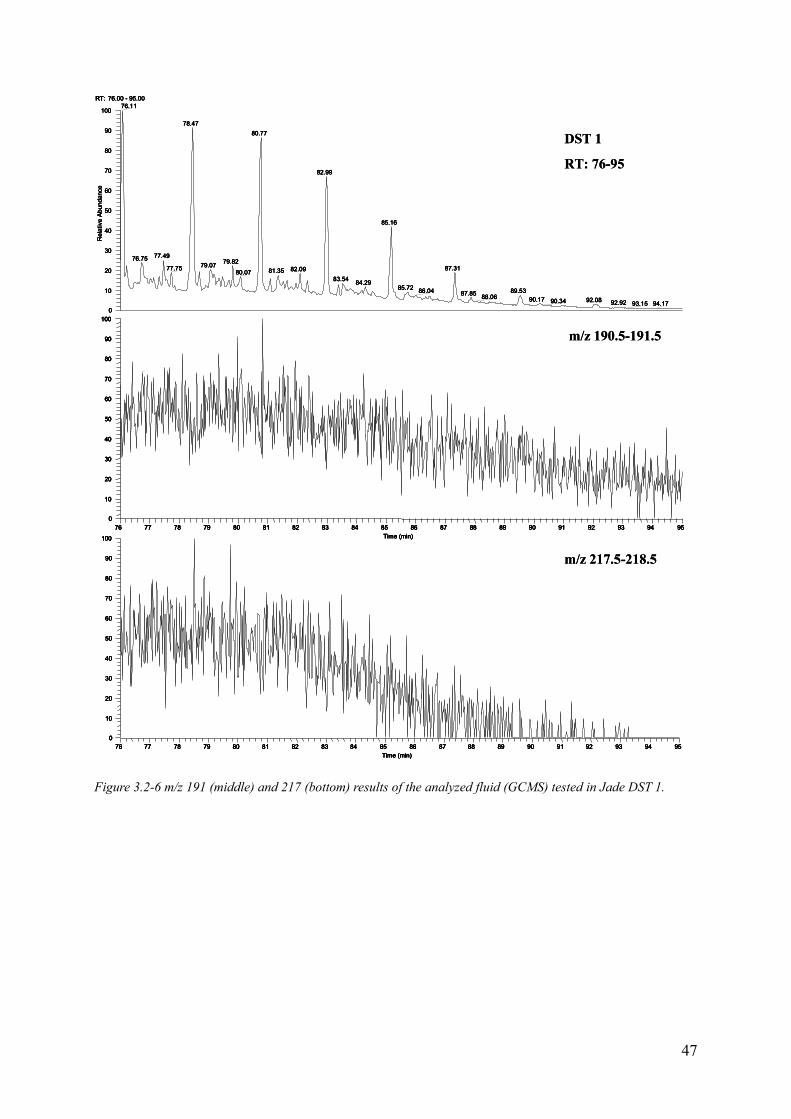
76 77 78 79 80 81 82 83 84 85 86 87 88 89 90 91 92 93 94 95Time (min)

0

10

20

30

40

50

60

70

80

90

100

RT: 76.00 - 95.00

76 77 78 79 80 81 82 83 84 85 86 87 88 89 90 91 92 93 94 95Time (min)

0

10

20

30

40

50

60

70

80

90

1000

10

20

30

40

50

60

70

80

90

100

Rel

ativ

e A

bund

ance

76.11

78.4780.77

82.99

85.16

77.4976.75 79.8279.0777.75 87.3182.0981.3580.0783.54 84.29

85.72 86.04 89.5387.85 88.06 90.17 92.0890.34 92.92 93.15 94.17

m/z 190.5-191.5

m/z 217.5-218.5

DST 1

RT: 76-95

76 77 78 79 80 81 82 83 84 85 86 87 88 89 90 91 92 93 94 95Time (min)

0

10

20

30

40

50

60

70

80

90

100

RT: 76.00 - 95.00

76 77 78 79 80 81 82 83 84 85 86 87 88 89 90 91 92 93 94 95Time (min)

0

10

20

30

40

50

60

70

80

90

1000

10

20

30

40

50

60

70

80

90

100

Rel

ativ

e A

bund

ance

76.11

78.4780.77

82.99

85.16

77.4976.75 79.8279.0777.75 87.3182.0981.3580.0783.54 84.29

85.72 86.04 89.5387.85 88.06 90.17 92.0890.34 92.92 93.15 94.17

76 77 78 79 80 81 82 83 84 85 86 87 88 89 90 91 92 93 94 95Time (min)

0

10

20

30

40

50

60

70

80

90

100

76 77 78 79 80 81 82 83 84 85 86 87 88 89 90 91 92 93 94 95Time (min)

0

10

20

30

40

50

60

70

80

90

100

76 77 78 79 80 81 82 83 84 85 86 87 88 89 90 91 92 93 94 95Time (min)

0

10

20

30

40

50

60

70

80

90

100

RT: 76.00 - 95.00

76 77 78 79 80 81 82 83 84 85 86 87 88 89 90 91 92 93 94 95Time (min)

0

10

20

30

40

50

60

70

80

90

1000

10

20

30

40

50

60

70

80

90

100

Rel

ativ

e A

bund

ance

76.11

78.4780.77

82.99

85.16

77.4976.75 79.8279.0777.75 87.3182.0981.3580.0783.54 84.29

85.72 86.04 89.5387.85 88.06 90.17 92.0890.34 92.92 93.15 94.17

RT: 76.00 - 95.00

76 77 78 79 80 81 82 83 84 85 86 87 88 89 90 91 92 93 94 95Time (min)

0

10

20

30

40

50

60

70

80

90

100

RT: 76.00 - 95.00

76 77 78 79 80 81 82 83 84 85 86 87 88 89 90 91 92 93 94 95Time (min)

0

10

20

30

40

50

60

70

80

90

1000

10

20

30

40

50

60

70

80

90

100

Rel

ativ

e A

bund

ance

76.11

78.4780.77

82.99

85.16

77.4976.75 79.8279.0777.75 87.3182.0981.3580.0783.54 84.29

85.72 86.04 89.5387.85 88.06 90.17 92.0890.34 92.92 93.15 94.17

m/z 190.5-191.5

m/z 217.5-218.5

DST 1

RT: 76-95

Figure 3.2-6 m/z 191 (middle) and 217 (bottom) results of the analyzed fluid (GCMS) tested in Jade DST 1.

47

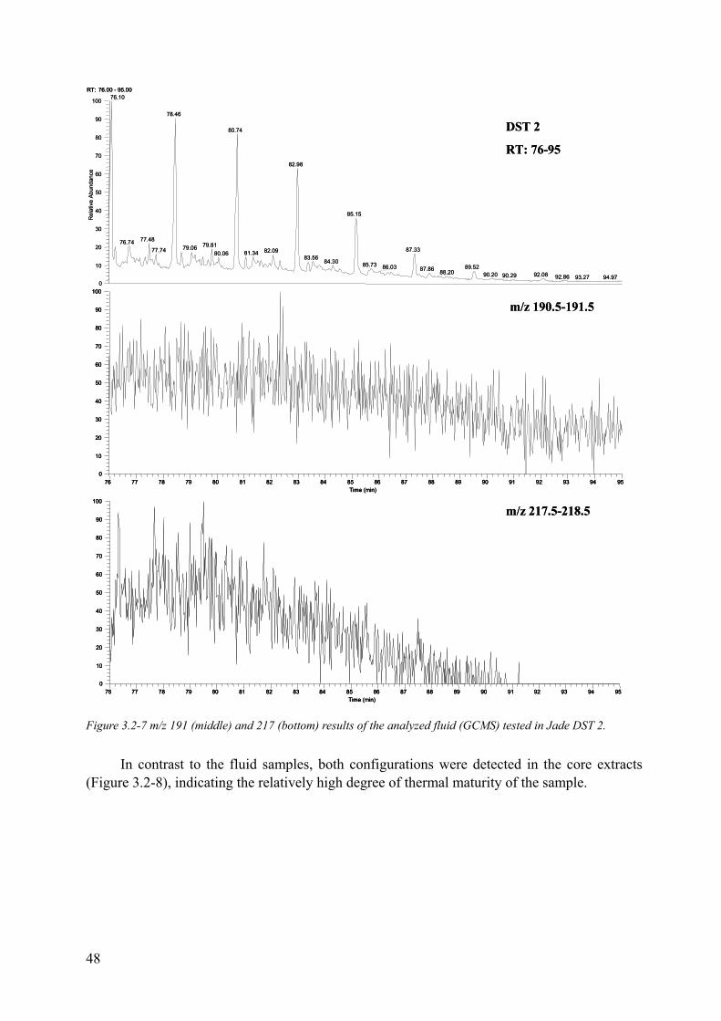
76 77 78 79 80 81 82 83 84 85 86 87 88 89 90 91 92 93 94 95Time (min)

0

10

20

30

40

50

60

70

80

90

100

RT: 76.00 - 95.00

76 77 78 79 80 81 82 83 84 85 86 87 88 89 90 91 92 93 94 95Time (min)

0

10

20

30

40

50

60

70

80

90

1000

10

20

30

40

50

60

70

80

90

100

Rel

ativ

e A

bund

ance

76.10

78.46

80.74

82.98

85.15

77.4876.74 79.8179.06 87.3377.74 82.0981.3480.0683.56

84.30 85.73 86.03 89.5287.86 88.20 90.20 92.0890.29 92.86 93.27 94.97

m/z 190.5-191.5

m/z 217.5-218.5

DST 2

RT: 76-95

76 77 78 79 80 81 82 83 84 85 86 87 88 89 90 91 92 93 94 95Time (min)

0

10

20

30

40

50

60

70

80

90

100

76 77 78 79 80 81 82 83 84 85 86 87 88 89 90 91 92 93 94 95Time (min)

0

10

20

30

40

50

60

70

80

90

100

RT: 76.00 - 95.00

76 77 78 79 80 81 82 83 84 85 86 87 88 89 90 91 92 93 94 95Time (min)

0

10

20

30

40

50

60

70

80

90

100

RT: 76.00 - 95.00

76 77 78 79 80 81 82 83 84 85 86 87 88 89 90 91 92 93 94 95Time (min)

0

10

20

30

40

50

60

70

80

90

1000

10

20

30

40

50

60

70

80

90

100

Rel

ativ

e A

bund

ance

76.10

78.46

80.74

82.98

85.15

77.4876.74 79.8179.06 87.3377.74 82.0981.3480.0683.56

84.30 85.73 86.03 89.5287.86 88.20 90.20 92.0890.29 92.86 93.27 94.97

m/z 190.5-191.5

m/z 217.5-218.5

DST 2

RT: 76-95

Figure 3.2-7 m/z 191 (middle) and 217 (bottom) results of the analyzed fluid (GCMS) tested in Jade DST 2.

In contrast to the fluid samples, both configurations were detected in the core extracts (Figure 3.2-8), indicating the relatively high degree of thermal maturity of the sample.

48

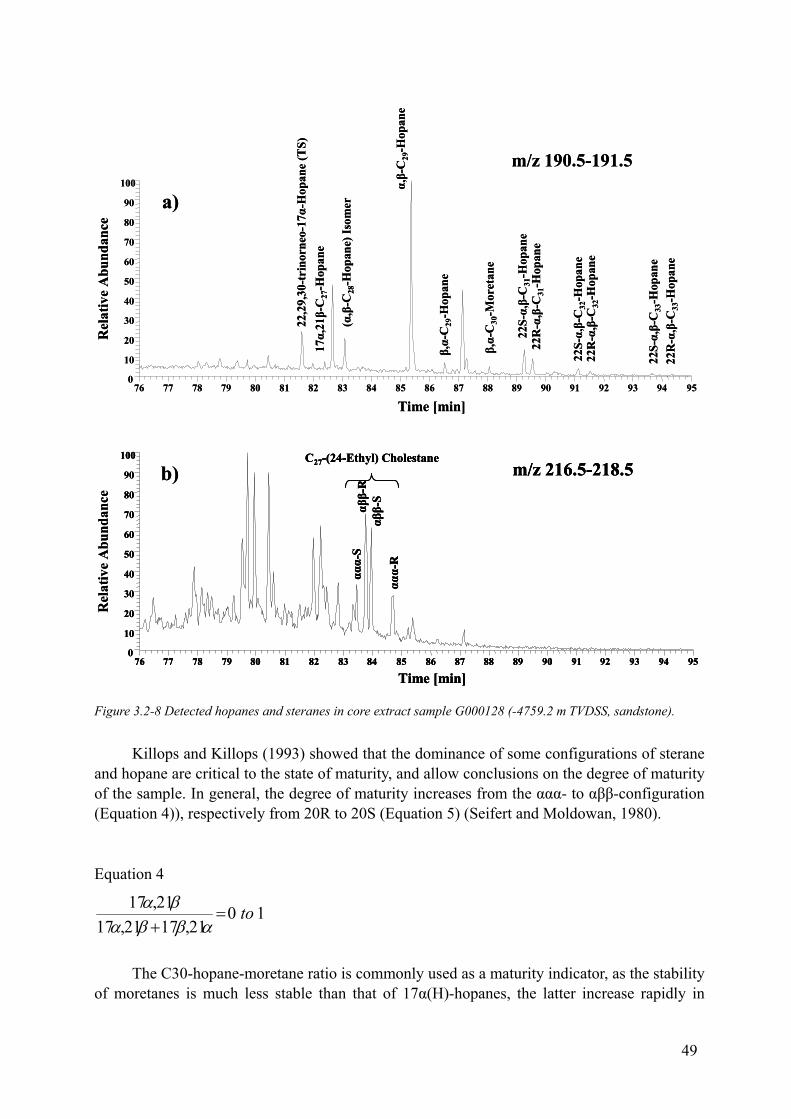
76 77 78 79 80 81 82 83 84 85 86 87 88 89 90 91 92 93 94 95

Time [min]

0

10

20

30

40

50

60

70

80

90

100

ααα-

S

αββ-

Sαββ-

R

ααα-

R

C27-(24-Ethyl) Cholestanem/z 216.5-218.5

76 77 78 79 80 81 82 83 84 85 86 87 88 89 90 91 92 93 94 95

Time [min]

0

10

20

30

40

50

60

70

80

90

100

22,2

9,30

-tri

norn

eo-1

7α-H

opan

e (T

S)17α,

21β-

C27

-Hop

ane

(α,β

-C28

-Hop

ane)

Isom

er

α,β-

C29

-Hop

ane

β,α-

C29

-Hop

ane

β,α-

C30

-Mor

etan

e

22S-α,β-

C31

-Hop

ane

22R

-α,β

-C31

-Hop

ane

22S-α,β-

C32

-Hop

ane

22R

-α,β

-C32

-Hop

ane

22S-α,β-

C33

-Hop

ane

22R

-α,β

-C33

-Hop

ane

m/z 190.5-191.5

a)

b)

Rel

ativ

e A

bund

ance

Rel

ativ

e A

bund

ance

76 77 78 79 80 81 82 83 84 85 86 87 88 89 90 91 92 93 94 95

Time [min]

0

10

20

30

40

50

60

70

80

90

100

ααα-

S

αββ-

Sαββ-

R

ααα-

R

C27-(24-Ethyl) Cholestanem/z 216.5-218.5

76 77 78 79 80 81 82 83 84 85 86 87 88 89 90 91 92 93 94 95

Time [min]

0

10

20

30

40

50

60

70

80

90

100

ααα-

S

αββ-

Sαββ-

R

ααα-

R

C27-(24-Ethyl) Cholestanem/z 216.5-218.5

76 77 78 79 80 81 82 83 84 85 86 87 88 89 90 91 92 93 94 95

Time [min]

0

10

20

30

40

50

60

70

80

90

100

22,2

9,30

-tri

norn

eo-1

7α-H

opan

e (T

S)17α,

21β-

C27

-Hop

ane

(α,β

-C28

-Hop

ane)

Isom

er

α,β-

C29

-Hop

ane

β,α-

C29

-Hop

ane

β,α-

C30

-Mor

etan

e

22S-α,β-

C31

-Hop

ane

22R

-α,β

-C31

-Hop

ane

22S-α,β-

C32

-Hop

ane

22R

-α,β

-C32

-Hop

ane

22S-α,β-

C33

-Hop

ane

22R

-α,β

-C33

-Hop

ane

m/z 190.5-191.5

a)

b)

Rel

ativ

e A

bund

ance

Rel

ativ

e A

bund

ance

Figure 3.2-8 Detected hopanes and steranes in core extract sample G000128 (-4759.2 m TVDSS, sandstone).

Killops and Killops (1993) showed that the dominance of some configurations of sterane and hopane are critical to the state of maturity, and allow conclusions on the degree of maturity of the sample. In general, the degree of maturity increases from the ααα- to αββ-configuration (Equation 4)), respectively from 20R to 20S (Equation 5) (Seifert and Moldowan, 1980).

Equation 4

1 021,1721,17

21,17 to=+ αββα

βα

The C30-hopane-moretane ratio is commonly used as a maturity indicator, as the stability of moretanes is much less stable than that of 17α(H)-hopanes, the latter increase rapidly in

49

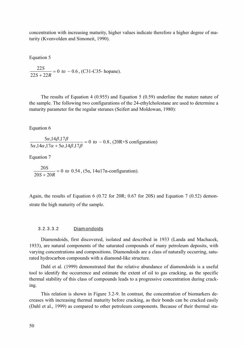
50

concentration with increasing maturity, higher values indicate therefore a higher degree of ma-turity (Kvenvolden and Simoneit, 1990).

Equation 5

0.6~ 02222

22 toRS

S=

+, (C31-C35- hopane).

The results of Equation 4 (0.955) and Equation 5 (0.59) underline the mature nature of the sample. The following two configurations of the 24-ethylcholestane are used to determine a maturity parameter for the regular steranes (Seifert and Moldowan, 1980):

Equation 6

0.8~ 017,14,517,14,5

17,14,5 to=+ ββαααα

ββα , (20R+S configuration)

Equation 7

.540 02020

20 toRS

S=

+, (5α, 14α17α-configuration).

Again, the results of Equation 6 (0.72 for 20R; 0.67 for 20S) and Equation 7 (0.52) demon-

strate the high maturity of the sample.

3.2.3.3.2 Diamondoids

Diamondoids, first discovered, isolated and described in 1933 (Landa and Machacek, 1933), are natural components of the saturated compounds of many petroleum deposits, with varying concentrations and compositions. Diamondoids are a class of naturally occurring, satu-rated hydrocarbon compounds with a diamond-like structure.

Dahl et al. (1999) demonstrated that the relative abundance of diamondoids is a useful tool to identify the occurrence and estimate the extent of oil to gas cracking, as the specific thermal stability of this class of compounds leads to a progressive concentration during crack-ing.

This relation is shown in Figure 3.2-9. In contrast, the concentration of biomarkers de-creases with increasing thermal maturity before cracking, as their bonds can be cracked easily (Dahl et al., 1999) as compared to other petroleum components. Because of their thermal sta-

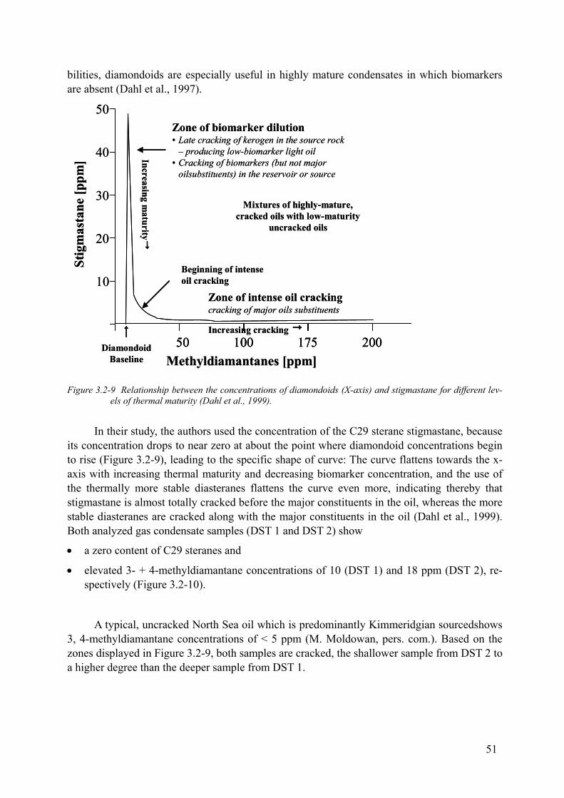
bilities, diamondoids are especially useful in highly mature condensates in which biomarkers are absent (Dahl et al., 1997).

Mixtures of highly-mature, cracked oils with low-maturity

uncracked oils

Zone of intense oil crackingcracking of major oils substituents

Increasing cracking 6

Zone of biomarker dilution• Late cracking of kerogen in the source rock

– producing low-biomarker light oil• Cracking of biomarkers (but not major

oilsubstituents) in the reservoir or source

Increasing maturity6

Methyldiamantanes [ppm]

Stig

mas

tane

[ppm

]

8Diamondoid

Baseline

Beginning of intense oil cracking

50

40

30

20

10

20017510050

Mixtures of highly-mature, cracked oils with low-maturity

uncracked oils

Zone of intense oil crackingcracking of major oils substituents

Increasing cracking 6

Zone of biomarker dilution• Late cracking of kerogen in the source rock

– producing low-biomarker light oil• Cracking of biomarkers (but not major

oilsubstituents) in the reservoir or source

Increasing maturity6

Methyldiamantanes [ppm]

Stig

mas

tane

[ppm

]

8Diamondoid

Baseline

Beginning of intense oil cracking

50

40

30

20

10

20017510050 20017510050

Figure 3.2-9 Relationship between the concentrations of diamondoids (X-axis) and stigmastane for different lev-els of thermal maturity (Dahl et al., 1999).

In their study, the authors used the concentration of the C29 sterane stigmastane, because its concentration drops to near zero at about the point where diamondoid concentrations begin to rise (Figure 3.2-9), leading to the specific shape of curve: The curve flattens towards the x-axis with increasing thermal maturity and decreasing biomarker concentration, and the use of the thermally more stable diasteranes flattens the curve even more, indicating thereby that stigmastane is almost totally cracked before the major constituents in the oil, whereas the more stable diasteranes are cracked along with the major constituents in the oil (Dahl et al., 1999). Both analyzed gas condensate samples (DST 1 and DST 2) show

• a zero content of C29 steranes and

• elevated 3- + 4-methyldiamantane concentrations of 10 (DST 1) and 18 ppm (DST 2), re-spectively (Figure 3.2-10).

A typical, uncracked North Sea oil which is predominantly Kimmeridgian sourcedshows 3, 4-methyldiamantane concentrations of < 5 ppm (M. Moldowan, pers. com.). Based on the zones displayed in Figure 3.2-9, both samples are cracked, the shallower sample from DST 2 to a higher degree than the deeper sample from DST 1.

51

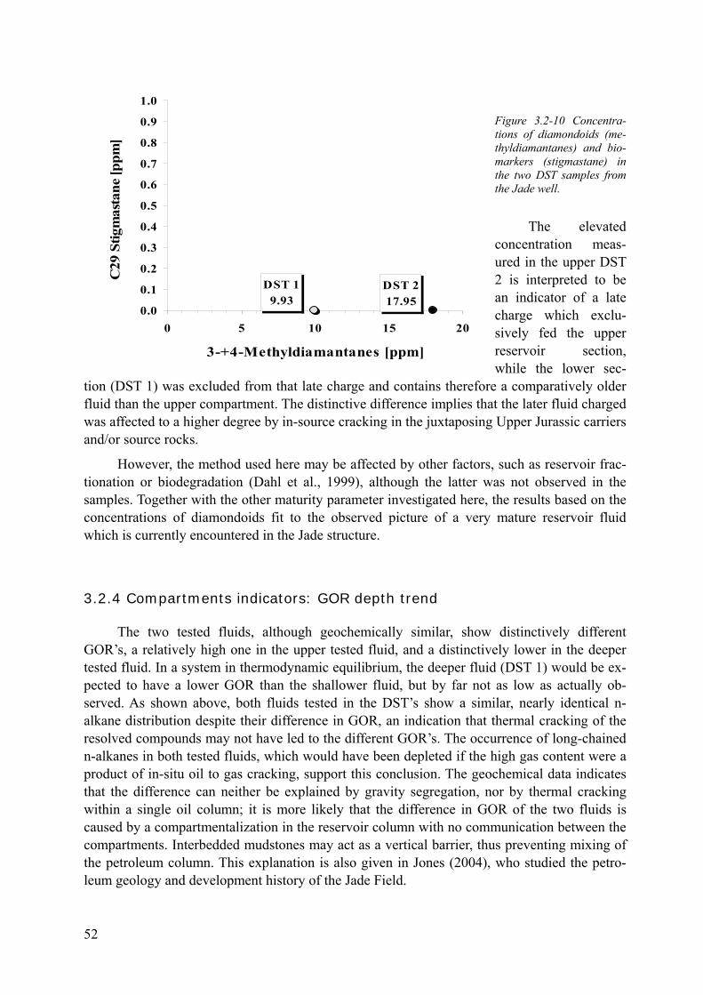
Figure 3.2-10 Concentra-tions of diamondoids (me-thyldiamantanes) and bio-markers (stigmastane) in the two DST samples from the Jade well.

The elevated concentration meas-ured in the upper DST 2 is interpreted to be an indicator of a late charge which exclu-sively fed the upper reservoir section, while the lower sec-

tion (DST 1) was excluded from that late charge and contains therefore a comparatively older fluid than the upper compartment. The distinctive difference implies that the later fluid charged was affected to a higher degree by in-source cracking in the juxtaposing Upper Jurassic carriers and/or source rocks.

DST 19.93

DST 217.95

0.0

0.1

0.2

0.3

0.4

0.5

0.6

0.7

0.8

0.9

1.0

0 5 10 15 20

3-+4-Methyldiamantanes [ppm]

C29

Stig

mas

tane

[ppm

]

However, the method used here may be affected by other factors, such as reservoir frac-tionation or biodegradation (Dahl et al., 1999), although the latter was not observed in the samples. Together with the other maturity parameter investigated here, the results based on the concentrations of diamondoids fit to the observed picture of a very mature reservoir fluid which is currently encountered in the Jade structure.

3.2.4 Compartments indicators: GOR depth trend

The two tested fluids, although geochemically similar, show distinctively different GOR’s, a relatively high one in the upper tested fluid, and a distinctively lower in the deeper tested fluid. In a system in thermodynamic equilibrium, the deeper fluid (DST 1) would be ex-pected to have a lower GOR than the shallower fluid, but by far not as low as actually ob-served. As shown above, both fluids tested in the DST’s show a similar, nearly identical n-alkane distribution despite their difference in GOR, an indication that thermal cracking of the resolved compounds may not have led to the different GOR’s. The occurrence of long-chained n-alkanes in both tested fluids, which would have been depleted if the high gas content were a product of in-situ oil to gas cracking, support this conclusion. The geochemical data indicates that the difference can neither be explained by gravity segregation, nor by thermal cracking within a single oil column; it is more likely that the difference in GOR of the two fluids is caused by a compartmentalization in the reservoir column with no communication between the compartments. Interbedded mudstones may act as a vertical barrier, thus preventing mixing of the petroleum column. This explanation is also given in Jones (2004), who studied the petro-leum geology and development history of the Jade Field.

52

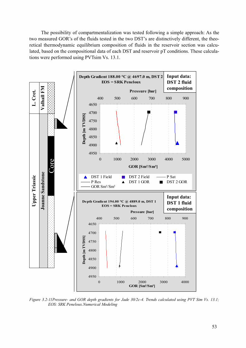
The possibility of compartmentalization was tested following a simple approach: As the two measured GOR’s of the fluids tested in the two DST’s are distinctively different, the theo-retical thermodynamic equilibrium composition of fluids in the reservoir section was calcu-lated, based on the compositional data of each DST and reservoir pT conditions. These calcula-tions were performed using PVTsim Vs. 13.1.

Joan

ne S

ands

tone

Val

hall

FM

Upp

er T

rias

sic

L. C

ret.

Cor

e

Depth Gradient 194.00 °C @ 4889.0 m, DST 1EOS = SRK Peneloux

4650

4700

4750

4800

4850

4900

4950

400 500 600 700 800 900

Pressure [bar]

Dep

th [m

TV

DSS

]

0 1000 2000 3000 4000GOR [Sm³/Sm³]

Depth Gradient 188.00 °C @ 4697.0 m, DST 2EOS = SRK Peneloux

4650

4700

4750

4800

4850

4900

4950

400 500 600 700 800 900

Pressure [bar]

Dep

th [m

TV

DSS

]

0 1000 2000 3000 4000 5000

GOR [Sm³/Sm³]

DST 1 Field DST 2 Field P SatP Res DST 1 GOR DST 2 GORGOR Sm³/Sm³

Input data: DST 2 fluid composition

Input data: DST 1 fluid composition Jo

anne

San

dsto

neV

alha

llFM

Upp

er T

rias

sic

L. C

ret.

Cor

e

Depth Gradient 194.00 °C @ 4889.0 m, DST 1EOS = SRK Peneloux

4650

4700

4750

4800

4850

4900

4950

400 500 600 700 800 900

Pressure [bar]

Dep

th [m

TV

DSS

]

0 1000 2000 3000 4000GOR [Sm³/Sm³]

Depth Gradient 188.00 °C @ 4697.0 m, DST 2EOS = SRK Peneloux

4650

4700

4750

4800

4850

4900

4950

400 500 600 700 800 900

Pressure [bar]

Dep

th [m

TV

DSS

]

0 1000 2000 3000 4000 5000

GOR [Sm³/Sm³]

DST 1 Field DST 2 Field P SatP Res DST 1 GOR DST 2 GORGOR Sm³/Sm³

Input data: DST 2 fluid composition

Input data: DST 1 fluid composition

Figure 3.2-11Pressure- and GOR depth gradients for Jade 30/2c-4. Trends calculated using PVT Sim Vs. 13.1; EOS: SRK Peneloux.Numerical Modeling

53

The result shows, that it is not possible to reproduce a continuous gradient using the available input data set, as the calculation predicts a distinctively higher GOR of about 2900 Sm³/Sm³ for the deeper DST 1 (upper graph in Figure 3.2-11), using the pressure and tempera-ture data of DST 2 as input data set. Also the calculation of equilibrium compositions based us-ing the deeper fluid as a starting point leads to similarly inaccurate results.

In the case of compartmentalization, it could be assumed that the lower DST 1 shows the composition and GOR of an isolated original fluid phase, while the shallower DST 2 shows contribution of a gas richer fluid from the deep, gas producing source rock intervals. However, the shaly layer responsible for the compartmentalization was either not sampled in the core, or the boundary lies elsewhere in the uncored section between the cored interval and tested inter-vals. Therefore, since the cored section in well 30/2c-4 between the two DST’s does not cover the complete Joanne Sandstone reservoir, is this assumption not provable.

The observed differences in GOR are most likely due to a higher methane input in the upper DST; both fluids are therefore highly similar, although not identical, and sourced by the same source rocks.

54

4 Numerical Modeling

4.1 Methods

The evolutionary history of a geologic sedimentary basin consists of a sequence of events in time during which a large number of physical processes have acted on the basin materials in three-dimensional space: It is the sum of all geological, geochemical and geophysical processes which have acted on its component parts throughout its geologic history (Poelchau et al., 1997). Sedimentary basins are the sites where petroleum is formed by chemical reactions from sedimentary biogenic precursor material, where it is redistributed by migration via permeable pathways, and where it is deposited and stored in reservoir rocks or dissipated and destroyed by chemical or biochemical reactions (Welte et al., 1997). The technique of basin modeling en-ables the user to address these processes. 3D basin modeling is today a standard in industrial studies dealing with hydrocarbon potential in sedimentary basins.

Pioneer work on hydrocarbon generation modeling was done by Tissot (1969), and since then, a variety of basin models were published. A detailed overview of the commercial side of basin modeling, including the most important features and properties of the individual basin modeling programs was given by Hermanrud (1993). A variety of models that aim at the quan-tifying hydrocarbon generation using basin modeling software have been developed in the early nineteen eighties; major publications here are from Bethke (1985), Durand (1984), Ler-che and Glezen (1984) and Welte and Yukler (1981).

Since the first introduction of numerical models (Deroo et al., 1969; Tissot, 1969), the technique of basin modeling has been greatly improved due to advances in organic geochemis-try, multi-phase fluid flow models, numerical methods and especially improved computer graphics and calculation power (Hermanrud, 1993; Young and Jackson, 1989). First, two-dimensional models were developed, which allowed simulating hydrocarbon migration pat-terns and pressure development through time. Because of the mainly convective pattern of mi-gration, the development shifted towards a three dimensional dynamic model which can de-scribe the behavior of a source rock during basin evolution by Welte (1972). Such a model was developed by IES (Germany). The model integrated the processes of fluid flow, compaction and heat transfer, and accurately predicted the generation of hydrocarbon in a sedimentary ba-sin. The most important aspects of this model are published in Welte (1997). In addition, there have been significant advances in the ability to describe and quantify the physical processes re-sponsible for the development of sedimentary basins and how these processes operate over a wide range of spatial and temporal scales.

A major advantage of 3D modeling is that the full relationship, spatial and temporal, be-tween the PSE’s is considered by constructing the three-dimensional geometry of the basin and its changes through time. In addition, 3D modeling enables volumetric calculations of trapped hydrocarbons for each time step. 3D basin modeling gives a dynamic view of processes such as sedimentation, compaction, water flow, heat transfer, source-rock maturation, petroleum expul-sion, migration and accumulation (Welte and Yukler, 1981), and aims at the prediction of fluid generation, migration and its compositional evolution by using kinetic schemes of hydrocarbon generation studied in detail by diverse laboratory tests, in other words, to test scientific as-

55

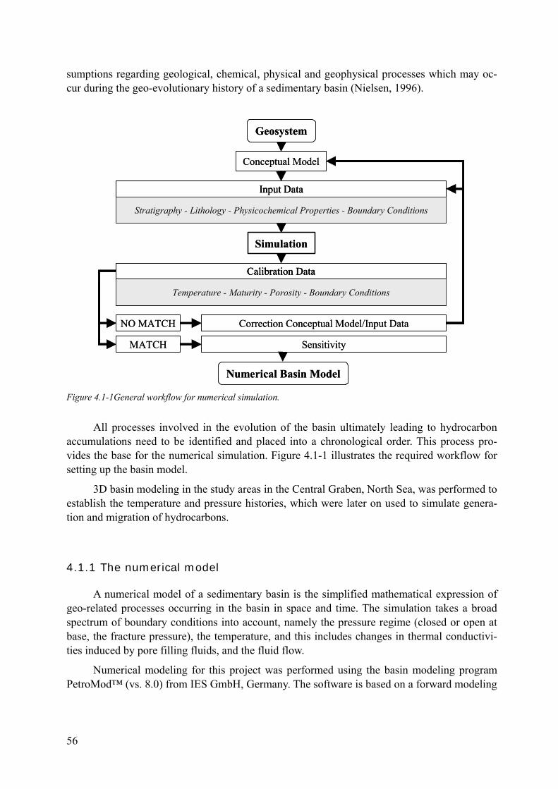
sumptions regarding geological, chemical, physical and geophysical processes which may oc-cur during the geo-evolutionary history of a sedimentary basin (Nielsen, 1996).

Conceptual Model

Simulation

MATCH

NO MATCH

Sensitivity

Correction Conceptual Model/Input Data

Input Data

Stratigraphy - Lithology - Physicochemical Properties - Boundary Conditions

Calibration Data

Temperature - Maturity - Porosity - Boundary Conditions

Geosystem

Numerical Basin Model

Conceptual Model

Simulation

MATCH

NO MATCH

Sensitivity

Correction Conceptual Model/Input Data

Input Data

Stratigraphy - Lithology - Physicochemical Properties - Boundary Conditions

Input Data

Stratigraphy - Lithology - Physicochemical Properties - Boundary Conditions

Calibration Data

Temperature - Maturity - Porosity - Boundary Conditions

Calibration Data

Temperature - Maturity - Porosity - Boundary Conditions

Geosystem

Numerical Basin Model

Figure 4.1-1General workflow for numerical simulation.

All processes involved in the evolution of the basin ultimately leading to hydrocarbon accumulations need to be identified and placed into a chronological order. This process pro-vides the base for the numerical simulation. Figure 4.1-1 illustrates the required workflow for setting up the basin model.

3D basin modeling in the study areas in the Central Graben, North Sea, was performed to establish the temperature and pressure histories, which were later on used to simulate genera-tion and migration of hydrocarbons.

4.1.1 The numerical model

A numerical model of a sedimentary basin is the simplified mathematical expression of geo-related processes occurring in the basin in space and time. The simulation takes a broad spectrum of boundary conditions into account, namely the pressure regime (closed or open at base, the fracture pressure), the temperature, and this includes changes in thermal conductivi-ties induced by pore filling fluids, and the fluid flow.

Numerical modeling for this project was performed using the basin modeling program PetroMod™ (vs. 8.0) from IES GmbH, Germany. The software is based on a forward modeling

56

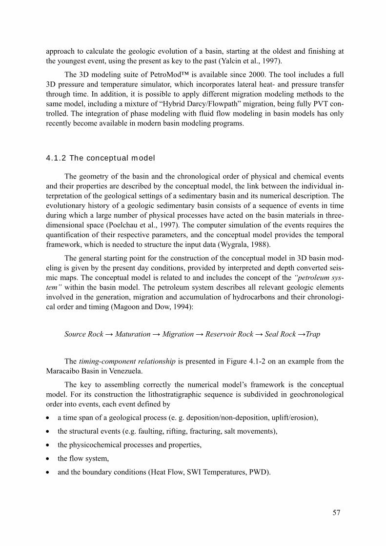
approach to calculate the geologic evolution of a basin, starting at the oldest and finishing at the youngest event, using the present as key to the past (Yalcin et al., 1997).

The 3D modeling suite of PetroMod™ is available since 2000. The tool includes a full 3D pressure and temperature simulator, which incorporates lateral heat- and pressure transfer through time. In addition, it is possible to apply different migration modeling methods to the same model, including a mixture of “Hybrid Darcy/Flowpath” migration, being fully PVT con-trolled. The integration of phase modeling with fluid flow modeling in basin models has only recently become available in modern basin modeling programs.

4.1.2 The conceptual model

The geometry of the basin and the chronological order of physical and chemical events and their properties are described by the conceptual model, the link between the individual in-terpretation of the geological settings of a sedimentary basin and its numerical description. The evolutionary history of a geologic sedimentary basin consists of a sequence of events in time during which a large number of physical processes have acted on the basin materials in three-dimensional space (Poelchau et al., 1997). The computer simulation of the events requires the quantification of their respective parameters, and the conceptual model provides the temporal framework, which is needed to structure the input data (Wygrala, 1988).

The general starting point for the construction of the conceptual model in 3D basin mod-eling is given by the present day conditions, provided by interpreted and depth converted seis-mic maps. The conceptual model is related to and includes the concept of the “petroleum sys-tem” within the basin model. The petroleum system describes all relevant geologic elements involved in the generation, migration and accumulation of hydrocarbons and their chronologi-cal order and timing (Magoon and Dow, 1994):

Source Rock → Maturation → Migration → Reservoir Rock → Seal Rock →Trap

timing-component relationship is presented in Figure 4.1-2The on an example from the Maracaibo Basin in Venezuela.

The key to assembling correctly the numerical model’s framework is the conceptual model. For its construction the lithostratigraphic sequence is subdivided in geochronological order into events, each event defined by

• a time span of a geological process (e. g. deposition/non-deposition, uplift/erosion),

• the structural events (e.g. faulting, rifting, fracturing, salt movements),

• the physicochemical processes and properties,

• the flow system,

• and the boundary conditions (Heat Flow, SWI Temperatures, PWD).

57

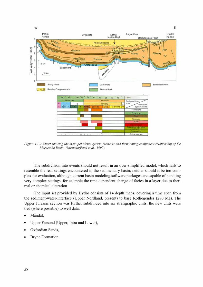
Figure 4.1-2 Chart showing the main petroleum system elements and their timing-component relationship of the Maracaibo Basin, Venezuela(Patel et al., 1997).

The subdivision into events should not result in an over-simplified model, which fails to resemble the real settings encountered in the sedimentary basin; neither should it be too com-plex for evaluation, although current basin modeling software packages are capable of handling very complex settings, for example the time dependent change of facies in a layer due to ther-mal or chemical alteration.

The input set provided by Hydro consists of 14 depth maps, covering a time span from the sediment-water-interface (Upper Nordland, present) to base Rotliegendes (280 Ma). The Upper Jurassic section was further subdivided into six stratigraphic units; the new units were tied (where possible) to well data:

• Mandal,

• Upper Farsund (Upper, Intra and Lower),

• Oxfordian Sands,

• Bryne Formation.

58

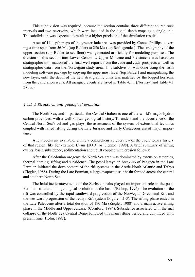
This subdivision was required, because the section contains three different source rock intervals and two reservoirs, which were included in the digital depth maps as a single unit. The subdivision was expected to result in a higher precision of the simulation results.

A set of 14 depth maps of the greater Jade area was provided by ConocoPhillips, cover-ing a time span from 56 Ma (top Balder) to 256 Ma (top Rotliegendes). The stratigraphy of the upper section (top Balder to sea floor) was generated artificially for modeling purposes. The division of this section into Lower Cenozoic, Upper Miocene and Pleistocene was based on stratigraphic information of the final well reports from the Jade and Judy prospects as well as stratigraphic data from the Norwegian study area. This subdivision was done using the basin modeling software package by copying the uppermost layer (top Balder) and manipulating the new layer, until the depth of the new stratigraphic units was matched by the logged horizons from the calibration wells. All assigned events are listed in Table 4.1 1 (Norway) and Table 4.1 2 (UK).

4.1.2.1 Structural and geological evolution

The North Sea, and in particular the Central Graben is one of the world’s major hydro-carbon provinces, with a well-known geological history. To understand the occurrence of the Central North Sea’s oil and gas plays, the assessment of the system of extensional tectonics coupled with failed rifting during the Late Jurassic and Early Cretaceous are of major impor-tance.

A few books are available, giving a comprehensive overview of the evolutionary history of that region, like for example Evans (2003) or Glennie (1998). A brief summary of rifting events, basin subsidence, sedimentation and uplift coupled with erosion follows:

After the Caledonian orogeny, the North Sea area was dominated by extension tectonics, thermal doming, rifting and subsidence. The post-Hercynian break-up of Pangaea in the Late Permian initiated the development of the rift systems in the Arctic-North Atlantic and Tethys (Ziegler, 1988). During the Late Permian, a large evaporitic salt basin formed across the central and southern North Sea.

The halokinetic movements of the Zechstein salts played an important role in the post-Permian structural and geological evolution of the basin (Bishop, 1996). The evolution of the rift was controlled by the rapid southward progression of the Norwegian-Greenland Rift and the westward progression of the Tethys Rift system (Figure 4.1-3). The rifting phase ended in the Late Paleocene after a total duration of 190 Ma (Ziegler, 1988) and a main active rifting phase in the Middle and Upper Jurassic (Cornford, 1994). Subsidence associated with thermal collapse of the North Sea Central Dome followed this main rifting period and continued until present time (Holm, 1998).

59

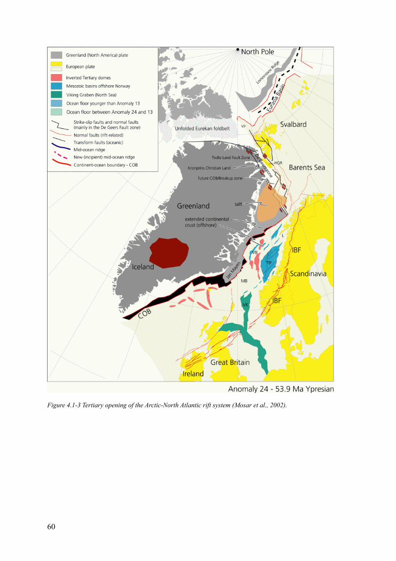
Figure 4.1-3 Tertiary opening of the Arctic-North Atlantic rift system (Mosar et al., 2002).

60

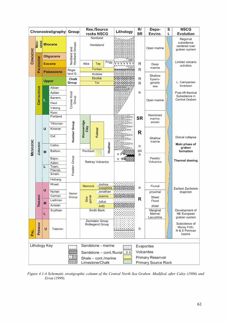
Figure 4.1-4 Schematic stratigraphic column of the Central North Sea Graben. Modified, after Caley (1986) and Errat (1999).

61

The geological history of the Central Graben is commonly divided into pre-, syn- and post-rift, according to the timing of the geological processes and its chronological order to the Upper Jurassic main rifting event.

4.1.2.1.1 Pre-rift (Permian to Middle Jurassic)

The Northern Permian Basin is the northern extension of the post-Variscian South Per-mian Basin, which extends from eastern England to the Russo-Polish border. Palynoflorical di-agnostics showed that both the Zechstein and Upper Rotliegendes of the North Sea basins were deposited within the latest stage of the Permian, the Tatarian (Glennie, 1998b). The Saalian Unconformity separates the Permian from the underlying Carboniferous. According to the lim-ited quantity of well data the thickness of the Rotliegend clastics ranges between 200 and 600 m (Ziegler, 1988) with rapid changes of thickness, which may indicate a depositional environ-ment of small rotated halfgrabens (Glennie, 1998b). The sedimentary facies are mainly fluvial, aeolian and sabkha.

The evolution of the inland Zechstein Sea within the Southern Permian basin was initi-ated by the progressive subsidence of the Norwegian-Greenland Rift and simultaneous rise of the sea level caused by the deglaciation of Gondwana (Ziegler, 1988). Thin Zechstein succes-sions are found on the Jaeren High and horsts within the Central Graben (Taylor, 1997). Avail-able seismic and well data indicates that the Central North Sea Graben did not start to subside during the Late Permian (Ziegler, 1988). Following the Zechstein transgressions several glacial induced sea level changes resulted in the cyclical deposition of carbonates and sulfates at the basin margins. A sharp drop in sea level caused the infill of the basin with the thick Stassfurt Salts (Z-2 salt), the basinal areas were characterized by relative shallow water depths. During the Tatarian epoch, the Arctic Seas withdrew from Northwest Europe (Ziegler, 1988).

During the Triassic, the Norwegian-Greenland Rift extended further to the South, enforc-ing the development of the primary features of the Viking and Central Graben, as well as the Moray Firth rifting system (Ziegler, 1988). A continued subsidence of the Northern and South-ern Permian basins as a result of lithospheric cooling and contraction is indicated by regional isopachs of the Triassic series (Sørensen, 1986). This subsidence, combined with rising sea level, led to the fully established connection of the Northern and Southern Permian basin, the Northwest European Basin (Ziegler, 1988). The Triassic Heron Group contains the major res-ervoirs of the UK study area.

During the Lower Jurassic the rift system remained active. As a consequence of wide-spread erosion resulting from post-depositional uplift during the Lower Jurassic, sedimental depositions of this epoch are seldom found in the Central Graben (Underhill, 1998a). The boundary between Lower and Middle Jurassic is locally marked by the Mid-Cimmerian Un-conformity, associated with a depositional shallowing, represented by widespread fluviodeltaic sediments, which form the reservoirs of the Fladen Group (Glennie, 1998c).

An accelerated crustal extension by the late Aalenian and Bajocian was accompanied by a large rift dome, centered below the Central Graben. The doming caused a truncation of the Permian and Mesozoic sediments in this region, which were partially eroded subaerially

62

(Ziegler, 1990). The erosion products form major oil reservoirs, mainly in the Viking Graben. Uplift movements of this Central North Sea Dome resulted in an enforced opening of the Cen-tral Graben, coupled with several sequences of volcanic activities, especially at the triple-junction of the three-armed rift system (Ziegler, 1988). Sedimentation was dominated by the paralic Pentland Formation, which overlies the Mid-Cimmerian Unconformity (Erratt et al., 1999).

Sea level reached a low stand in the Aalenian-Bajocian. During the late Bajocian-Bathonian, the Central North Sea Dome began to subside slowly. The occurrence of a thick continental clastic series in the North Sea Central Graben indicates that sedimentation still con-tinued (Ziegler, 1990b). During the progressing Middle Jurassic, the rising sea level induced together with the continued crustal extension a further subsidence of the graben area.

4.1.2.1.2 Syn-rift (Middle to Upper Jurassic)

During the late Middle and Upper Jurassic the Viking and Central Graben developed into the dominant rift system (Ziegler, 1988). As a result of continued crustal expansion and the subsidence of the former site of the North Sea Central Dome, deep marine sediments were in-troduced for the first time into the Central Graben (Underhill, 1998b).

The Upper Jurassic was a period of eustatic sea level rise. The Upper Jurassic marine transgression progressed throughout the Kimmeridgian (Erratt et al., 1999). A widespread sedimentation of organic-rich shales of Kimmeridgian and Tithonian age occurred in the Cen-tral North Sea area. These shales form the major source rocks for the hydrocarbon accumul-tions of the Viking and Central Graben, the Kimmeridge Shale Formation respectively its Norwegian equivalents like the Mandal or Draupne Formation (Figure 4.1-7).

Between the middle Oxfordian to early Kimmeridgian, a main rifting period influenced strongly the graben system (Rattey and Hayward, 1993), which deepened the basins in all three arms. The results are more apparent in the Viking Graben, with the development of a subma-rine relief of several 1000 m, than in the Central Graben, where much of the tensional deforma-tion of the pre-Permian level was balanced by plastic deformation of the Zechstein salts (Ziegler, 1988).

At the former site of the subsiding Central North Sea Dome, a widespread deposition of the sediments of the Humber Group took place (Glennie, 1998a). The water depth at this point of time did not exceed 100 m, since the distal lower shoreface facies of the Fulmar Formation, the major reservoir unit of the Central Graben, and its equivalent, the offshore silts of the Heather Formation, do not show any indication of deep water facies (Erratt et al., 1999). This time of extension caused the development of a major fault system with destruction and tilting of the earlier sedimentary sequences.

The origin of the Cimmerian unconformity is most likely related to the combined effects of rapid subsidence of the rift areas and significant drop of the relative sea level (Vail, 1981). After the late Kimmeridgian rifting event, the rate of tectonic activities declined steadily (Oakman and Partington, 1998).

63

4.1.2.1.3 Post-rift (Early Cretaceous to present)

After the main active rifting phase of the Central Graben, thermal subsidence started and continued more or less uninterrupted until present times (Holm, 1998).

During the Early Cretaceous, global sea level rise caused the deposition of deep water shales and locally pelagic carbonates, which filled the relief of the continued subsiding rift area, as well as the flooding of great parts of the platforms (Oakman and Partington, 1998). The western sub-basins of the Central Graben are characterized by reactivation along only a part of their pre-Cretaceous extent (Erratt et al., 1999), including a reorientation of the existing strike direction of the fault system.

In the Upper Cretaceous chalks and marls of the Chalk Group filled gradually the Viking and Central Graben, with sedimentation rates exceeding subsidence rates (Ziegler, 1988). Many of the Lower Cretaceous faults die out within the Upper Cretaceous strata, only the ma-jor faults remain. Although global sea level was rising, water depth decreased until Maas-trichtian. During the Upper Cretaceous, crustal stretching played only a secondary role, re-gional downwarping being more related to lithospheric cooling (Ziegler, 1988).

The latest Paleocene and early Eocene were marked by a regional transgression, induced by the succeeding subsidence of the North Sea Basin in combination with rising sea levels. Consequence was a reduction of the deposition of sandy sediments and an enforced sedimenta-tion of pelagic shale facies. During the Oligocene the sea level reached a low stand, and the sedimentation- and subsidence rates were in equilibrium (Ziegler, 1988).

The sedimentation patterns in the Central Graben during the Miocene and Pliocene were strongly influenced by repeated sea level changes. After the Miocene, sedimentation rates were higher than subsidence rates, with a thickness of the Cenozoic sediments in the middle of the basin along the graben axis of about 3.5 km. The result was a progressive shallowing of the Central North Sea. After the early Tertiary fragmentation of the Eurasian-North American crustal plate, the Mesozoic rift system of the North Sea Basin became inactive (Ziegler, 1988).

4.1.2.1.4 Halokinetic movements

According to Jackson (1986), salt behaves as a fluid with no variations of density due to stress. Therefore no minimum stress is necessary in order to trigger the movement of the salt, if its density is lower than the density of the overburden. Salt movements can be initiated or re-tarded by regional stress. In general, the depth which is regarded as starting depth for the rise of salt by buoyancy lies between 600 and 1000 m, depending of the density of the overlying sediments (Taylor, 1998).

Figure 4.1-5Important features in the central and southern North Sea are salt structures ( ). During the Mesozoic and Cenozoic the pattern of sedimentation and deformation within the Central Graben was strongly influenced by the underlying Permian salt basin (Hodgson et al., 1992). Earliest diapirism of the Zechstein salts started in Triassic times, initiated along exten-sional faults (Davison et al., 2000). The movement of these salts is partly responsible for the trapping of petroleum (Taylor, 1998). At the tops of the diapirs, good-quality channel sand-

64

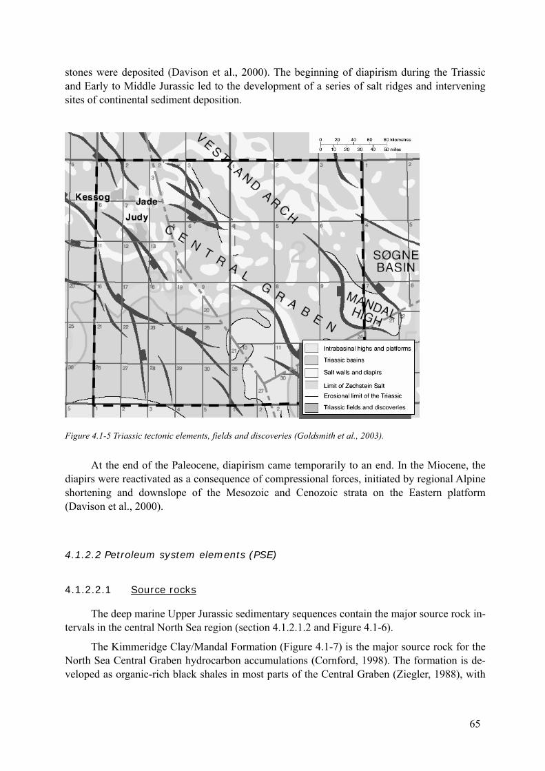
stones were deposited (Davison et al., 2000). The beginning of diapirism during the Triassic and Early to Middle Jurassic led to the development of a series of salt ridges and intervening sites of continental sediment deposition.

Figure 4.1-5 Triassic tectonic elements, fields and discoveries (Goldsmith et al., 2003).

At the end of the Paleocene, diapirism came temporarily to an end. In the Miocene, the diapirs were reactivated as a consequence of compressional forces, initiated by regional Alpine shortening and downslope of the Mesozoic and Cenozoic strata on the Eastern platform (Davison et al., 2000).

4.1.2.2 Petroleum system elements (PSE)

4.1.2.2.1 Source rocks

The deep marine Upper Jurassic sedimentary sequences contain the major source rock in-tervals in the central North Sea region (section 4.1.2.1.2 and Figure 4.1-6).

Figure 4.1-7The Kimmeridge Clay/Mandal Formation ( ) is the major source rock for the North Sea Central Graben hydrocarbon accumulations (Cornford, 1998). The formation is de-veloped as organic-rich black shales in most parts of the Central Graben (Ziegler, 1988), with

65

burial depths between 2000 m to more than 5000 m, and a maximum thickness of about 1200 m (Holm, 1998).

Figure 4.1-6 Distribution of Upper Jurassic source rocks and major discoveries (Fraser et al., 2003).

The organic-rich facies represents marine hemipelagic deposition in an an-oxic environment. The Bathonian to Mid-dle Oxfordian Heather/Farsund Formation has a higher terrigenous input than the overlying Kimmeridge Clay/Mandal For-mation. The formation consists of gray, silty mudstones, with interbedded good-quality shoreface sandstones. The Heather/Farsund Formation is an effective seal for many Middle Jurassic reservoirs, and is, where developed in an argillaceous

facies, a “fair” to “good” gas-prone source rock mixed kerogen (types II/III, average TOC of about 2-4%, but has only “poor” oil-prone source rock quality (Johnson and Fisher, 1998; Ku-bala et al., 2003).

010203040506070

<2 2-3 3-4 4-5 5-6 6-7 7-8 >8

TOC [%] range

Freq

uenc

y

80

Kimmeridge Clay (331 wells) Heather (170 wells)

Farsund Formation

Pentland Fm.

HeatherFm.

Fulm

ar F

m.

Kimmeridge Clay Formation

Fulmar Fm

.

N UK S

Mandal Formation

Tyne

Gro

up

Haugesund Formation

UlaFm.

W Norway E

Central Graben

Farsund FormationFarsund Formation

Pentland Fm.

HeatherFm.

Fulm

ar F

m.

Kimmeridge Clay Formation

Fulmar Fm

.

N UK S

Mandal Formation

Tyne

Gro

upTy

ne G

roup

Haugesund Formation

UlaFm.

W Norway EW Norway E

Central Graben

010203040506070

<2 2-3 3-4 4-5 5-6 6-7 7-8 >8

TOC [%] range

Freq

uenc

y

80

Kimmeridge Clay (331 wells) Heather (170 wells)

Farsund Formation

Pentland Fm.

HeatherFm.

Fulm

ar F

m.

Kimmeridge Clay Formation

Fulmar Fm

.

N UK S

Mandal Formation

Tyne

Gro

up

Haugesund Formation

UlaFm.

W Norway E

Central Graben

Farsund FormationFarsund Formation

Pentland Fm.

HeatherFm.

Fulm

ar F

m.

Kimmeridge Clay Formation

Fulmar Fm

.

N UK S

Mandal Formation

Tyne

Gro

upTy

ne G

roup

Haugesund Formation

UlaFm.

W Norway EW Norway E

Central Graben

Figure 4.1-7 Left: Upper Jurassic Central Graben nomenclature (modified, after Vollset and Doré (1984)). Right: Histogram of total organic matter for the Kimmeridge Clays and the Heather Formation in the Central North Sea (Kubala et al., 2003).

The Middle Jurassic (Aalenian to Bajocian) fluvial deposits of the Pentland/Bryne For-mation (Fladden Group), overlain by the marine strata of the Heather Formation, consist of

66

coal-bearing heterolithic carbonaceous sandstones and shales, containing type III organic mat-ter (Donovan, 1993; Underhill, 1998b). The average cumulative coal thickness is low; coaly units (carbargillites) may reach values up to 30% TOC.

4.1.2.2.2 Reservoir rocks

4.1.2.2.2.1 Rotliegendes

The UK study area does not contain proven hydrocarbon accumulations in the members of the Rotliegendes Group. In the Norwegian study area, confirmed Rotliegendes plays are lo-cated in the Embla Field (block 2/7); traps are basically rotated fault blocks and sandstone res-ervoirs of predominantly continental origin.

4.1.2.2.2.2 Triassic

The major economic interest in Triassic reservoirs lies in their potential for deep gas condensates. The reservoir quality in these Triassic sandstones is highly variable, controlled by primary depositional facies, diagenesis and overpressure development. The main reservoir in-tervals consist of thick, fluvial dominated sandstones (Johnson and Fisher, 1998), deposited in terrestrial, semiarid environments. Fluvial channels and sheetflood deposits are common. The lithostratigraphy of the Triassic period in the Central Graben is subdivided into the Smith Bank Formation (Skythian), and the members of the Heron Group, the Skagerrak Formation (Anisian to Norian) and the Marmock Formation (Rhaetian). The climate during deposition of the Skagerrak Formation, the major production zone, was arid to semi-arid, as manifested by inter-fingering evaporitic deposits. The presence of caliche also indicates a relatively hot climate with low seasonal rainfall (Weibel, 1998). The sedimentation of Triassic sediments was strongly controlled by halokinetic movements of Zechstein salts during the period of thermal subsidence of the graben (Fisher and Mudge, 1998; Johnson and Fisher, 1998). The complex thickness pattern, including sudden thickness changes are due to the partial absence of fine-grained fluvial and sheetflood sandstones in areas of salt-induced topographic lows, caused by salt withdrawal or dissolution (Fisher and Mudge, 1998).

The Skagerrak Group is divided into two sandstone members (Joanne & Judy) and two mudstone members, the Jonathan and the Julius members. The sandstone members of the Skagerrak Formation consist basically of very fine to fine silty sandstones or locally medium grained sandstones, with interbedded mudstones and the sporadic appearance of conglomer-ates. The sandstones are commonly part of fining-upward sequences, for example in the stacked fluvial channel and sheetflood sandstone facies, interbedded with shales. According to Fisher and Mudge (1998) the reservoir quality of the Skagerrak Formation is commonly poor, with low net to gross ratios, poor lateral continuity and high intra-reservoir sedimentological complexity, but the reservoir quality can essentially differ from this generalized description, depending of the three quality controlling factors: primary depositional facies, diagenesis and overpressure development.

67

4.1.2.2.2.3 Jurassic

Upper Jurassic reservoirs were deposited during a punctuated transgression. The deposi-tion of shales is regarded as a time of widespread marine flooding, while sandstone deposition represents lows of relative sea level (Underhill, 1998b). Due to the syn-depositional rifting and locally involved salt movements is the distribution and predictability of the Upper Jurassic plays very complex (Johnson and Fisher, 1998).

During the Late Jurassic, when sedimentary sequences like the Humber Group were de-posited, the North Sea region was affected by a significant phase of extensional activities (Underhill, 1998b), concentrated on the three rift arms of the Central Graben area. The activi-ties had a major impact on the style of deposition, resulting in the development of fault frag-ments on the tilted fault blocks. This led to erosion of the foot wall areas and accumulation of very coarse grained clastic sediments in the basin margins. A simultaneous rise of the relative sea level led to the development of an extensive shelf environment with shallow-marine, high-quality sandstone deposits (Johnson and Fisher, 1998). In the Central Graben, those shallow-marine deposits overlie transgressively Triassic deposits. Upper Jurassic sandstones, deposited simultaneously with rifting in the Central Graben, form major reservoirs for many fields, with traps being either stratigraphic or structural. These syn-rift reservoirs include both shallow-marine and deep-marine/fan sandstones (Johnson and Fisher, 1998), locally interfingering with the source rock shales (Carr, 2001).

4.1.2.2.2.4 Cretaceous

The deposition of the Upper Cretaceous reservoir units reflects the post-rift subsidence of the graben system below, with depositions of combined Upper Cretaceous and Tertiary sedi-ments reaching locally 4000 m of thickness (Johnson and Fisher, 1998). Main Cretaceous oil producing formations in the Norwegian Central Graben are the Ekofisk Formation of Danian age and the Maastrichtian Tor Formation. In addition, the Campanian-Turonian Hod Forma-tion, like the Tor Formation a member of the Chalk Group, is an important reservoir for many of the Central Graben plays (Hughes et al., 1985).

Cretaceous plays were confirmed by the giant Ekofisk Field, the Valhall, Hod, Tor and Edda fields and several other discoveries. The trap types are halokinetic and stratigraphic. The best reservoir properties (e.g. porosities of 20-30%) within the Chalk Group are found in the up to 250 m thick reworked chalk facies, e.g. those of the Tor and Ekofisk formations (Underhill, 1998b). The migration and trapping mechanism remain poorly understood (Underhill, 2003). The open marine, allochthonous chalks were deposited mostly by turbidity currents or slumps, which destructed early diagenetic cements and enhanced thereby reservoir qualities (Schatzinger, 1985).

Holm (1998) stated that the preservation of the enhanced porosities depends highly on overpressure development. The reservoirs of the Chalk Group are sourced by the Upper Juras-sic shale (Mandal- and Draupne Formation) and Lower - Middle Jurassic shale and coal of the Bryne Formation.

68

4.1.2.2.3 Seals

The preservation of an overpressured cell is mostly controlled through the integrity of its lateral and vertical seals. In order to obtain overpressured conditions, pressure buildup must be at least equal to pressure loss through the seals. The Central Graben traps include fault blocks draped with Jurassic mudstones, Cretaceous chalk, or shale of Tertiary age. In contrast to the Viking Graben and Moray Firth, salt tectonics is responsible for much of the structural com-plexity that provides opportunities for hydrocarbon entrapment. Stratigraphic traps are domi-nant in the Upper Jurassic and younger sandstones. Seals are Jurassic shale, Cretaceous chalk, or Tertiary shale. The Cromer Knoll Group is composed of argillaceous marls and claystones, and is commonly regarded as seals for the underlying pre-Cretaceous overpressured sedimen-tary sequences (Holm, 1998).

4.1.3 Input data

The numerical model requires an input data set being assigned to the different events of the model. While events are defined in terms of their duration as part of the conceptual model, the properties of the corresponding layers are defined in terms of age, thickness, lithology, in-cluding lithology type and physical properties, such as permeability, compressibility, heat ca-pacity, thermal conductivity, etc. (Poelchau et al., 1997). This is the most crucial point during the setup of the model, as the quantity of available data obtained from direct observations is usually insufficient to describe the real system in detail. This means that input data are to a large extent based on assumptions made by the modeler.

The standard data available in the modeling software contain information about litholo-gies and models of various types, including kinetic reactions, fluid components, relative per-meability relationships and others.

In addition, thermal boundaries for the model and properties for the petroleum system elements are defined. Together, those parameters outline the direction the simulation is taking.

4.1.3.1 Lithologies and ages of events

The mechanical change of the lithology through time is defined via its changes of poros-ity, permeability and density, the thermal properties through thermal conductivity and capacity. Most of the parameters change continuously through time, some even interact. Besides the de-fault lithologies available in PetroMod™, the software allows the definition of user-defined lithologies, either via input in a spreadsheet, or via mixing of two or more default lithologies. The new lithology will receive ratio-dependent physical properties.

Petrophysical parameters available by default do not necessarily fit to those lithologies which are actually present in the basin. Tagging a unit as a “chalk” means, that this unit will be defined in the model for the simulation as a rock with the average petrophysical values of a chalk, but as the lithological unit present in the basin is not necessarily average, a different name tag could fit much better to this unit. This mislabeling can be avoided by including petrophysical parameters obtained from measurements performed at this peculiar unit. If no

69

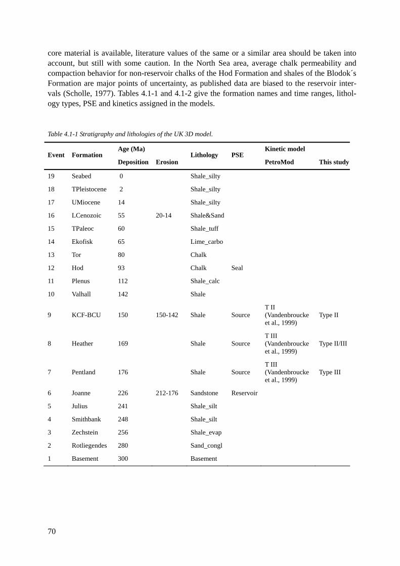
70

core material is available, literature values of the same or a similar area should be taken into account, but still with some caution. In the North Sea area, average chalk permeability and compaction behavior for non-reservoir chalks of the Hod Formation and shales of the Blodok´s Formation are major points of uncertainty, as published data are biased to the reservoir inter-vals (Scholle, 1977). Tables 4.1-1 and 4.1-2 give the formation names and time ranges, lithol-ogy types, PSE and kinetics assigned in the models.

Table 4.1-1 Stratigraphy and lithologies of the UK 3D model.

Age (Ma) Kinetic model Event Formation

Deposition Erosion Lithology PSE

PetroMod This study

19 Seabed 0 Shale_silty

18 TPleistocene 2 Shale_silty

17 UMiocene 14 Shale_silty

16 LCenozoic 55 20-14 Shale&Sand

15 TPaleoc 60 Shale_tuff

14 Ekofisk 65 Lime_carbo

13 Tor 80 Chalk

12 Hod 93 Chalk Seal

11 Plenus 112 Shale_calc

10 Valhall 142 Shale

9 KCF-BCU 150 150-142 Shale Source T II (Vandenbroucke et al., 1999)

Type II

8 Heather 169 Shale Source T III (Vandenbroucke et al., 1999)

Type II/III

7 Pentland 176 Shale Source T III (Vandenbroucke et al., 1999)

Type III

6 Joanne 226 212-176 Sandstone Reservoir

5 Julius 241 Shale_silt

4 Smithbank 248 Shale_silt

3 Zechstein 256 Shale_evap

2 Rotliegendes 280 Sand_congl

1 Basement 300 Basement

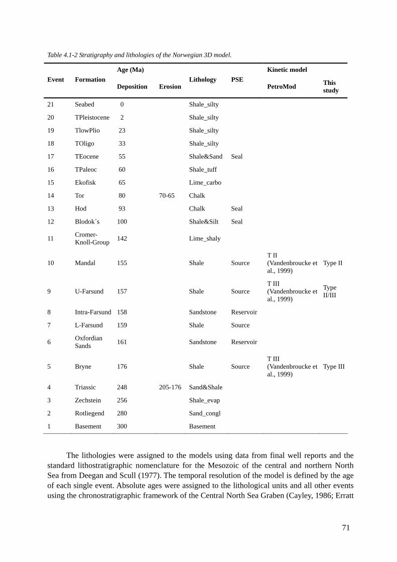
71

Table 4.1-2 Stratigraphy and lithologies of the Norwegian 3D model.

Age (Ma) Kinetic model Event Formation

Deposition Erosion Lithology PSE

PetroMod This study

21 Seabed 0 Shale_silty

20 TPleistocene 2 Shale_silty

19 TlowPlio 23 Shale_silty

18 TOligo 33 Shale_silty

17 TEocene 55 Shale&Sand Seal

16 TPaleoc 60 Shale_tuff

15 Ekofisk 65 Lime_carbo

14 Tor 80 70-65 Chalk

13 Hod 93 Chalk Seal

12 Blodok´s 100 Shale&Silt Seal

11 Cromer-Knoll-Group 142 Lime_shaly

10 Mandal 155 Shale Source T II (Vandenbroucke et al., 1999)

Type II

9 U-Farsund 157 Shale Source T III (Vandenbroucke et al., 1999)

Type II/III

8 Intra-Farsund 158 Sandstone Reservoir

7 L-Farsund 159 Shale Source

6 Oxfordian Sands 161 Sandstone Reservoir

5 Bryne 176 Shale Source T III (Vandenbroucke et al., 1999)

Type III

4 Triassic 248 205-176 Sand&Shale

3 Zechstein 256 Shale_evap

2 Rotliegend 280 Sand_congl

1 Basement 300 Basement

The lithologies were assigned to the models using data from final well reports and the standard lithostratigraphic nomenclature for the Mesozoic of the central and northern North Sea from Deegan and Scull (1977). The temporal resolution of the model is defined by the age of each single event. Absolute ages were assigned to the lithological units and all other events using the chronostratigraphic framework of the Central North Sea Graben (Cayley, 1986; Erratt

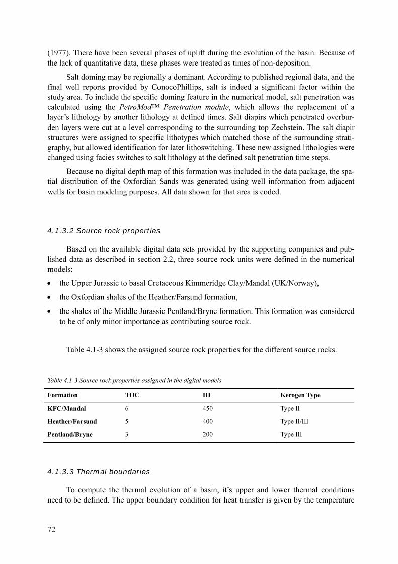
(1977). There have been several phases of uplift during the evolution of the basin. Because of the lack of quantitative data, these phases were treated as times of non-deposition.

Salt doming may be regionally a dominant. According to published regional data, and the final well reports provided by ConocoPhillips, salt is indeed a significant factor within the study area. To include the specific doming feature in the numerical model, salt penetration was calculated using the PetroMod™ Penetration module, which allows the replacement of a layer’s lithology by another lithology at defined times. Salt diapirs which penetrated overbur-den layers were cut at a level corresponding to the surrounding top Zechstein. The salt diapir structures were assigned to specific lithotypes which matched those of the surrounding strati-graphy, but allowed identification for later lithoswitching. These new assigned lithologies were changed using facies switches to salt lithology at the defined salt penetration time steps.

Because no digital depth map of this formation was included in the data package, the spa-tial distribution of the Oxfordian Sands was generated using well information from adjacent wells for basin modeling purposes. All data shown for that area is coded.

4.1.3.2 Source rock properties

Based on the available digital data sets provided by the supporting companies and pub-lished data as described in section 2.2, three source rock units were defined in the numerical models:

• the Upper Jurassic to basal Cretaceous Kimmeridge Clay/Mandal (UK/Norway),

• the Oxfordian shales of the Heather/Farsund formation,

• the shales of the Middle Jurassic Pentland/Bryne formation. This formation was considered to be of only minor importance as contributing source rock.

Table 4.1-3 shows the assigned source rock properties for the different source rocks.

Table 4.1-3 Source rock properties assigned in the digital models.

Formation TOC HI Kerogen Type

KFC/Mandal 6 450 Type II

Heather/Farsund 5 400 Type II/III

Pentland/Bryne 3 200 Type III

4.1.3.3 Thermal boundaries

To compute the thermal evolution of a basin, it’s upper and lower thermal conditions need to be defined. The upper boundary condition for heat transfer is given by the temperature

72

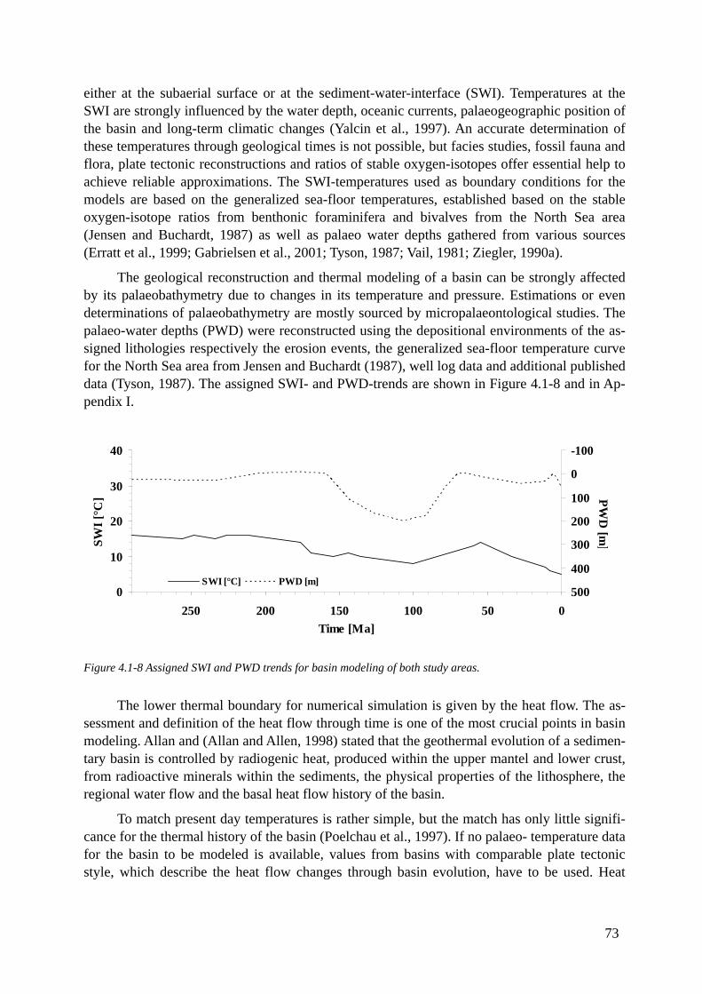
73

either at the subaerial surface or at the sediment-water-interface (SWI). Temperatures at the SWI are strongly influenced by the water depth, oceanic currents, palaeogeographic position of the basin and long-term climatic changes (Yalcin et al., 1997). An accurate determination of these temperatures through geological times is not possible, but facies studies, fossil fauna and flora, plate tectonic reconstructions and ratios of stable oxygen-isotopes offer essential help to achieve reliable approximations. The SWI-temperatures used as boundary conditions for the models are based on the generalized sea-floor temperatures, established based on the stable oxygen-isotope ratios from benthonic foraminifera and bivalves from the North Sea area (Jensen and Buchardt, 1987) as well as palaeo water depths gathered from various sources (Erratt et al., 1999; Gabrielsen et al., 2001; Tyson, 1987; Vail, 1981; Ziegler, 1990a).

The geological reconstruction and thermal modeling of a basin can be strongly affected by its palaeobathymetry due to changes in its temperature and pressure. Estimations or even determinations of palaeobathymetry are mostly sourced by micropalaeontological studies. The palaeo-water depths (PWD) were reconstructed using the depositional environments of the as-signed lithologies respectively the erosion events, the generalized sea-floor temperature curve for the North Sea area from Jensen and Buchardt (1987), well log data and additional published data (Tyson, 1987). The assigned SWI- and PWD-trends are shown in Figure 4.1-8 and in Ap-pendix I.

0

10

20

30

40

050100150200250Time [Ma]

SWI [

°C]

-100

0

100

200

300

400

500

PWD

[m]

SWI [°C] PWD [m]

Figure 4.1-8 Assigned SWI and PWD trends for basin modeling of both study areas.

The lower thermal boundary for numerical simulation is given by the heat flow. The as-sessment and definition of the heat flow through time is one of the most crucial points in basin modeling. Allan and (Allan and Allen, 1998) stated that the geothermal evolution of a sedimen-tary basin is controlled by radiogenic heat, produced within the upper mantel and lower crust, from radioactive minerals within the sediments, the physical properties of the lithosphere, the regional water flow and the basal heat flow history of the basin.

To match present day temperatures is rather simple, but the match has only little signifi-cance for the thermal history of the basin (Poelchau et al., 1997). If no palaeo- temperature data for the basin to be modeled is available, values from basins with comparable plate tectonic style, which describe the heat flow changes through basin evolution, have to be used. Heat

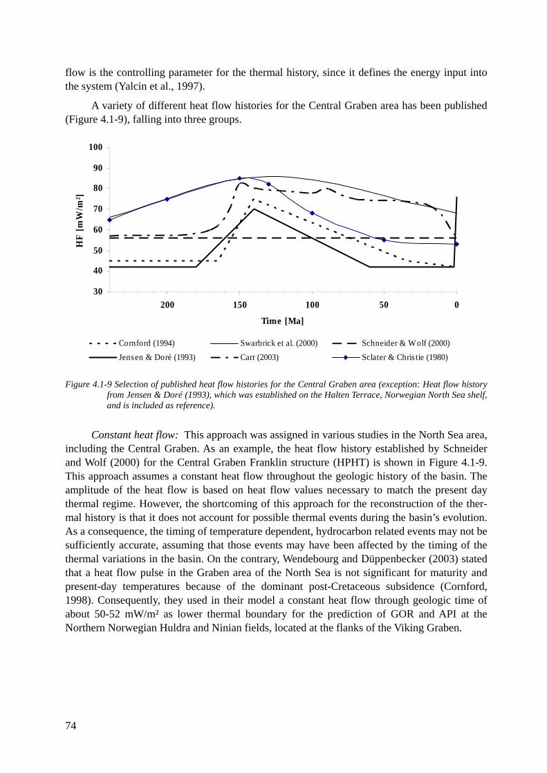
74

flow is the controlling parameter for the thermal history, since it defines the energy input into the system (Yalcin et al., 1997).

A variety of different heat flow histories for the Central Graben area has been published (Figure 4.1-9), falling into three groups.

30

40

50

60

70

80

90

100

050100150200

Time [Ma]

HF

[mW

/m²]

Cornford (1994) Swarbrick et al. (2000) Schneider & Wolf (2000)Jensen & Doré (1993) Carr (2003) Sclater & Chris tie (1980)

Figure 4.1-9 Selection of published heat flow histories for the Central Graben area (exception: Heat flow history from Jensen & Doré (1993), which was established on the Halten Terrace, Norwegian North Sea shelf, and is included as reference).

Constant heat flow: This approach was assigned in various studies in the North Sea area, including the Central Graben. As an example, the heat flow history established by Schneider and Wolf (2000) for the Central Graben Franklin structure (HPHT) is shown in Figure 4.1-9. This approach assumes a constant heat flow throughout the geologic history of the basin. The amplitude of the heat flow is based on heat flow values necessary to match the present day thermal regime. However, the shortcoming of this approach for the reconstruction of the ther-mal history is that it does not account for possible thermal events during the basin’s evolution. As a consequence, the timing of temperature dependent, hydrocarbon related events may not be sufficiently accurate, assuming that those events may have been affected by the timing of the thermal variations in the basin. On the contrary, Wendebourg and Düppenbecker (2003) stated that a heat flow pulse in the Graben area of the North Sea is not significant for maturity and present-day temperatures because of the dominant post-Cretaceous subsidence (Cornford, 1998). Consequently, they used in their model a constant heat flow through geologic time of about 50-52 mW/m² as lower thermal boundary for the prediction of GOR and API at the Northern Norwegian Huldra and Ninian fields, located at the flanks of the Viking Graben.

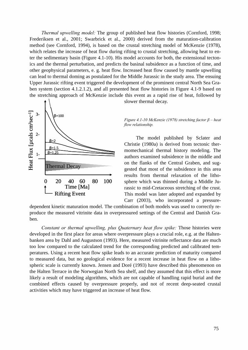
75

Thermal upwelling model: The group of published heat flow histories (Cornford, 1998; Frederiksen et al., 2001; Swarbrick et al., 2000) derived from the maturation-calibration method (see Cornford, 1994), is based on the crustal stretching model of McKenzie (1978), which relates the increase of heat flow during rifting to crustal stretching, allowing heat to en-ter the sedimentary basin (Figure 4.1-10). His model accounts for both, the extensional tecton-ics and the thermal perturbation, and predicts the basinal subsidence as a function of time, and other geophysical parameters, e. g. heat flow. Increased heat flow caused by mantle upwelling can lead to thermal doming as postulated for the Middle Jurassic in the study area. The ensuing Upper Jurassic rifting event triggered the development of the prominent central North Sea Gra-ben system (section 4.1.2.1.2), and all presented heat flow histories in Figure 4.1-9 based on the stretching approach of McKenzie include this event as a rapid rise of heat, followed by

slower thermal decay.

Figure 4.1-10 McKenzie (1978) stretching factor β – heat flow relationship.

The model published by Sclater and Christie (1980a) is derived from tectonic ther-momechanical thermal history modeling. The authors examined subsidence in the middle and on the flanks of the Central Graben, and sug-gested that most of the subsidence in this area results from thermal relaxation of the litho-sphere which was thinned during a Middle Ju-rassic to mid-Cretaceous stretching of the crust. This model was later adopted and expanded by Carr (2003), who incorporated a pressure-

dependent kinetic maturation model. The combination of both models was used to correctly re-produce the measured vitrinite data in overpressured settings of the Central and Danish Gra-ben.

Constant or thermal upwelling, plus Quaternary heat flow spike: Those histories were developed in the first place for areas where overpressure plays a crucial role, e.g. at the Halten-banken area by Dahl and Augustson (1993). Here, measured vitrinite reflectance data are much too low compared to the calculated trend for the corresponding predicted and calibrated tem-peratures. Using a recent heat flow spike leads to an accurate prediction of maturity compared to measured data, but no geological evidence for a recent increase in heat flow on a litho-spheric scale is currently known. Jensen and Doré (1993) have described this phenomenon on the Halten Terrace in the Norwegian North Sea shelf, and they assumed that this effect is more likely a result of modeling algorithms, which are not capable of handling rapid burial and the combined effects caused by overpressure properly, and not of recent deep-seated crustal activities which may have triggered an increase of heat flow.

Hea

t Flu

x [µ

cals

cm

²sec

-1]

3-

2-

1-

Time [Ma]0 20 40 60 80 100

β=1.25

β=100

β=1.5

β=2

Rifting Event

Thermal DecayHea

t Flu

x [µ

cals

cm

²sec

-1]

3-

2-

1-

Time [Ma]0 20 40 60 80 100

β=1.25

β=100

β=1.5

β=2

Rifting Event

Thermal Decay

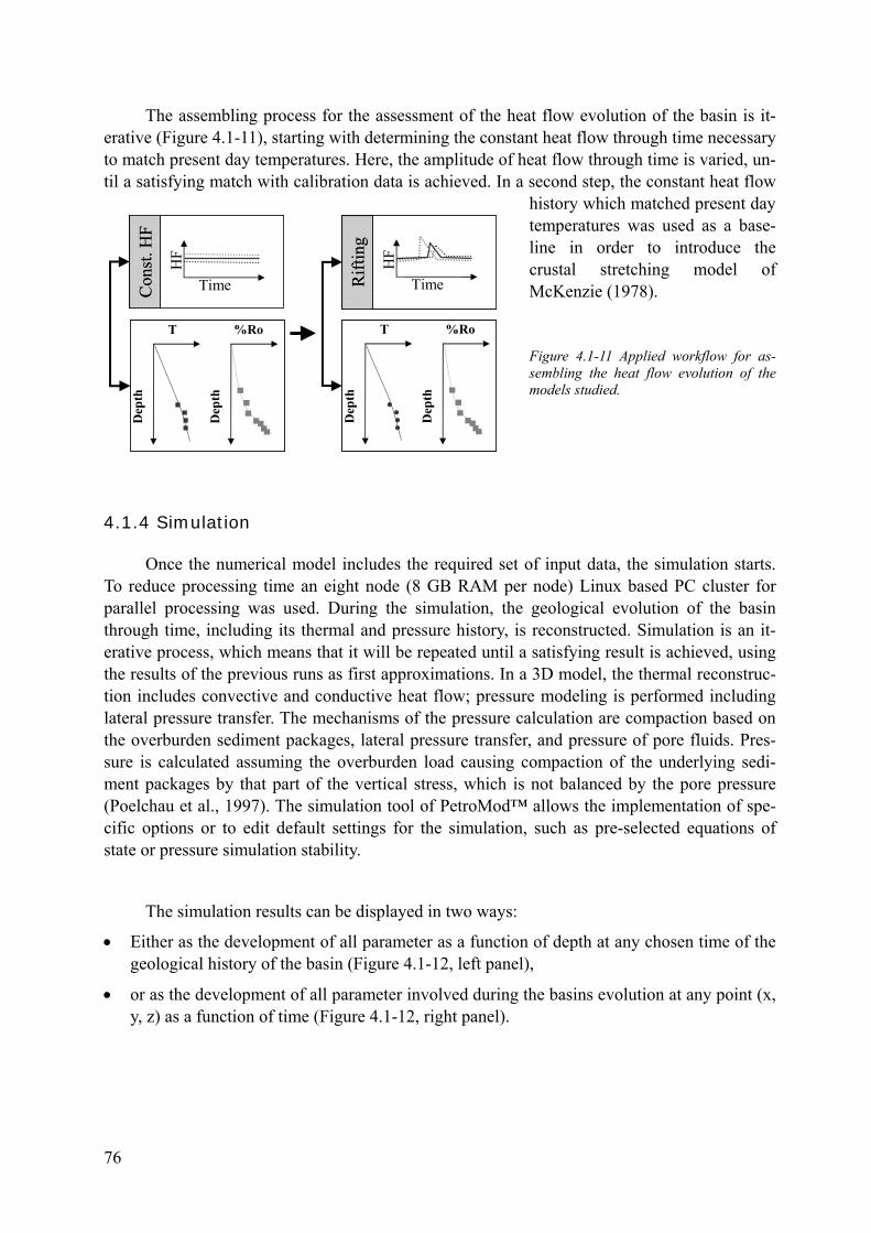
The assembling process for the assessment of the heat flow evolution of the basin is it-erative (Figure 4.1-11), starting with determining the constant heat flow through time necessary to match present day temperatures. Here, the amplitude of heat flow through time is varied, un-til a satisfying match with calibration data is achieved. In a second step, the constant heat flow

history which matched present day temperatures was used as a base-line in order to introduce the crustal stretching model of McKenzie (1978).

HF

TimeCon

st. H

F

T

Dep

th

%Ro

Dep

th

HF

TimeRift

ing

TD

epth

%Ro

Dep

th

HF

TimeCon

st. H

F

HF

TimeCon

st. H

F

T

Dep

th

%Ro

Dep

th

T

Dep

th

%Ro

Dep

th

HF

TimeRift

ing

HF

TimeRift

ing

TD

epth

%Ro

Dep

th

TD

epth

%Ro

Dep

th

Figure 4.1-11 Applied workflow for as-sembling the heat flow evolution of the models studied.

4.1.4 Simulation

Once the numerical model includes the required set of input data, the simulation starts. To reduce processing time an eight node (8 GB RAM per node) Linux based PC cluster for parallel processing was used. During the simulation, the geological evolution of the basin through time, including its thermal and pressure history, is reconstructed. Simulation is an it-erative process, which means that it will be repeated until a satisfying result is achieved, using the results of the previous runs as first approximations. In a 3D model, the thermal reconstruc-tion includes convective and conductive heat flow; pressure modeling is performed including lateral pressure transfer. The mechanisms of the pressure calculation are compaction based on the overburden sediment packages, lateral pressure transfer, and pressure of pore fluids. Pres-sure is calculated assuming the overburden load causing compaction of the underlying sedi-ment packages by that part of the vertical stress, which is not balanced by the pore pressure (Poelchau et al., 1997). The simulation tool of PetroMod™ allows the implementation of spe-cific options or to edit default settings for the simulation, such as pre-selected equations of state or pressure simulation stability.

The simulation results can be displayed in two ways:

• Either as the development of all parameter as a function of depth at any chosen time of the geological history of the basin (Figure 4.1-12, left panel),

• or as the development of all parameter involved during the basins evolution at any point (x, y, z) as a function of time (Figure 4.1-12, right panel).

76

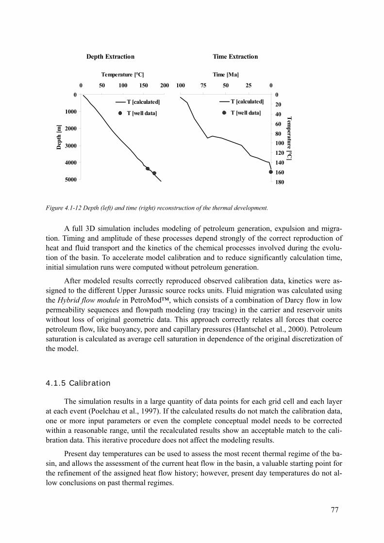
Depth Extraction

0

1000

2000

3000

4000

5000

0 50 100 150 200

Temperature [°C]

Dep

th [m

]

T [calculated]

T [well data]

Time Extraction

020406080100120140160180

0255075100

Time [Ma]

Tem

perature [°C]

T [calculated]

T [well data]

Figure 4.1-12 Depth (left) and time (right) reconstruction of the thermal development.

A full 3D simulation includes modeling of petroleum generation, expulsion and migra-tion. Timing and amplitude of these processes depend strongly of the correct reproduction of heat and fluid transport and the kinetics of the chemical processes involved during the evolu-tion of the basin. To accelerate model calibration and to reduce significantly calculation time, initial simulation runs were computed without petroleum generation.

After modeled results correctly reproduced observed calibration data, kinetics were as-signed to the different Upper Jurassic source rocks units. Fluid migration was calculated using the Hybrid flow module in PetroMod™, which consists of a combination of Darcy flow in low permeability sequences and flowpath modeling (ray tracing) in the carrier and reservoir units without loss of original geometric data. This approach correctly relates all forces that coerce petroleum flow, like buoyancy, pore and capillary pressures (Hantschel et al., 2000). Petroleum saturation is calculated as average cell saturation in dependence of the original discretization of the model.

4.1.5 Calibration

The simulation results in a large quantity of data points for each grid cell and each layer at each event (Poelchau et al., 1997). If the calculated results do not match the calibration data, one or more input parameters or even the complete conceptual model needs to be corrected within a reasonable range, until the recalculated results show an acceptable match to the cali-bration data. This iterative procedure does not affect the modeling results.

Present day temperatures can be used to assess the most recent thermal regime of the ba-sin, and allows the assessment of the current heat flow in the basin, a valuable starting point for the refinement of the assigned heat flow history; however, present day temperatures do not al-low conclusions on past thermal regimes.

77

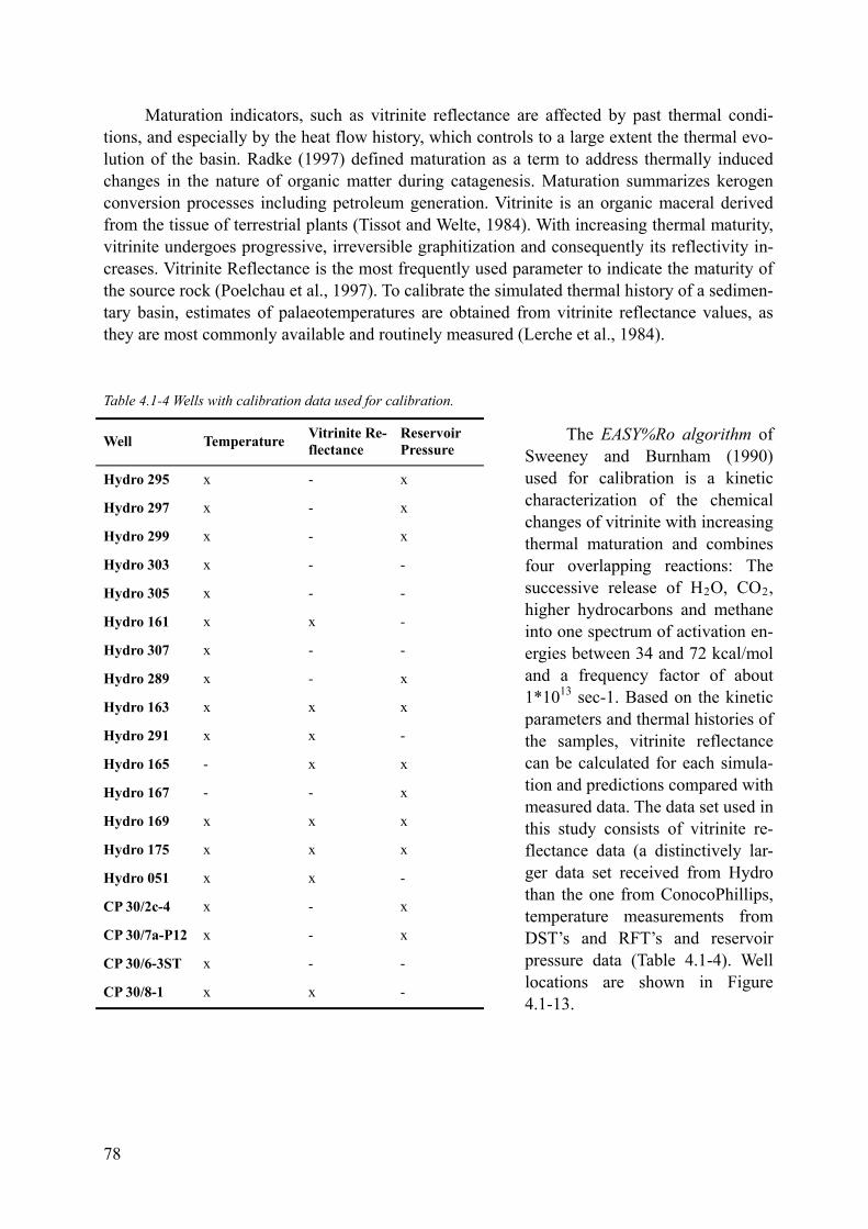
Maturation indicators, such as vitrinite reflectance are affected by past thermal condi-tions, and especially by the heat flow history, which controls to a large extent the thermal evo-lution of the basin. Radke (1997) defined maturation as a term to address thermally induced changes in the nature of organic matter during catagenesis. Maturation summarizes kerogen conversion processes including petroleum generation. Vitrinite is an organic maceral derived from the tissue of terrestrial plants (Tissot and Welte, 1984). With increasing thermal maturity, vitrinite undergoes progressive, irreversible graphitization and consequently its reflectivity in-creases. Vitrinite Reflectance is the most frequently used parameter to indicate the maturity of the source rock (Poelchau et al., 1997). To calibrate the simulated thermal history of a sedimen-tary basin, estimates of palaeotemperatures are obtained from vitrinite reflectance values, as they are most commonly available and routinely measured (Lerche et al., 1984).

Table 4.1-4 Wells with calibration data used for calibration.

EASY%Ro algorithmThe of Sweeney and Burnham (1990) used for calibration is a kinetic characterization of the chemical changes of vitrinite with increasing thermal maturation and combines four overlapping reactions: The successive release of H2O, CO2, higher hydrocarbons and methane into one spectrum of activation en-ergies between 34 and 72 kcal/mol and a frequency factor of about 1*1013 sec-1. Based on the kinetic parameters and thermal histories of the samples, vitrinite reflectance can be calculated for each simula-tion and predictions compared with measured data. The data set used in this study consists of vitrinite re-flectance data (a distinctively lar-ger data set received from Hydro than the one from ConocoPhillips, temperature measurements from DST’s and RFT’s and reservoir pressure data (Table 4.1-4). Well locations are shown in Figure 4.1-13.

Well Temperature Vitrinite Re-flectance

Reservoir Pressure

Hydro 295 x - x

Hydro 297 x - x

Hydro 299 x - x

Hydro 303 x - -

Hydro 305 x - -

Hydro 161 x x -

Hydro 307 x - -

Hydro 289 x - x

Hydro 163 x x x

Hydro 291 x x -

Hydro 165 - x x

Hydro 167 - - x

Hydro 169 x x x

Hydro 175 x x x

Hydro 051 x x -

CP 30/2c-4 x - x

CP 30/7a-P12 x - x

CP 30/6-3ST x - -

CP 30/8-1 x x -

78

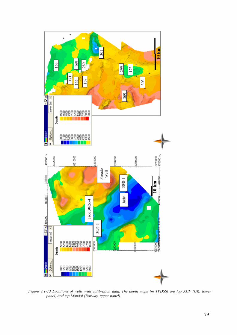
309

167

169

16517

1

299

173

301

289

303

163

10 k

m

Judy

Jade

30/

2c-4

Pseu

doW

ell

30/8

-1

30/6

-3

10 k

m

309

167

169

16517

1

299

173

301

289

303

163

10 k

m

309

167

169

16517

1

299

173

301

289

303

163

309

167

169

16517

1

299

173

301

289

303

163

10 k

m10

km

Judy

Jade

30/

2c-4

Pseu

doW

ell

30/8

-1

30/6

-3

10 k

m

Judy

Jade

30/

2c-4

Pseu

doW

ell

30/8

-1

30/6

-3

Judy

Jade

30/

2c-4

Pseu

doW

ell

30/8

-1

30/6

-3

10 k

m10

km

Figure 4.1-13 Locations of wells with calibration data. The depth maps (m TVDSS) are top KCF (UK, lower

panel) and top Mandal (Norway, upper panel).

79

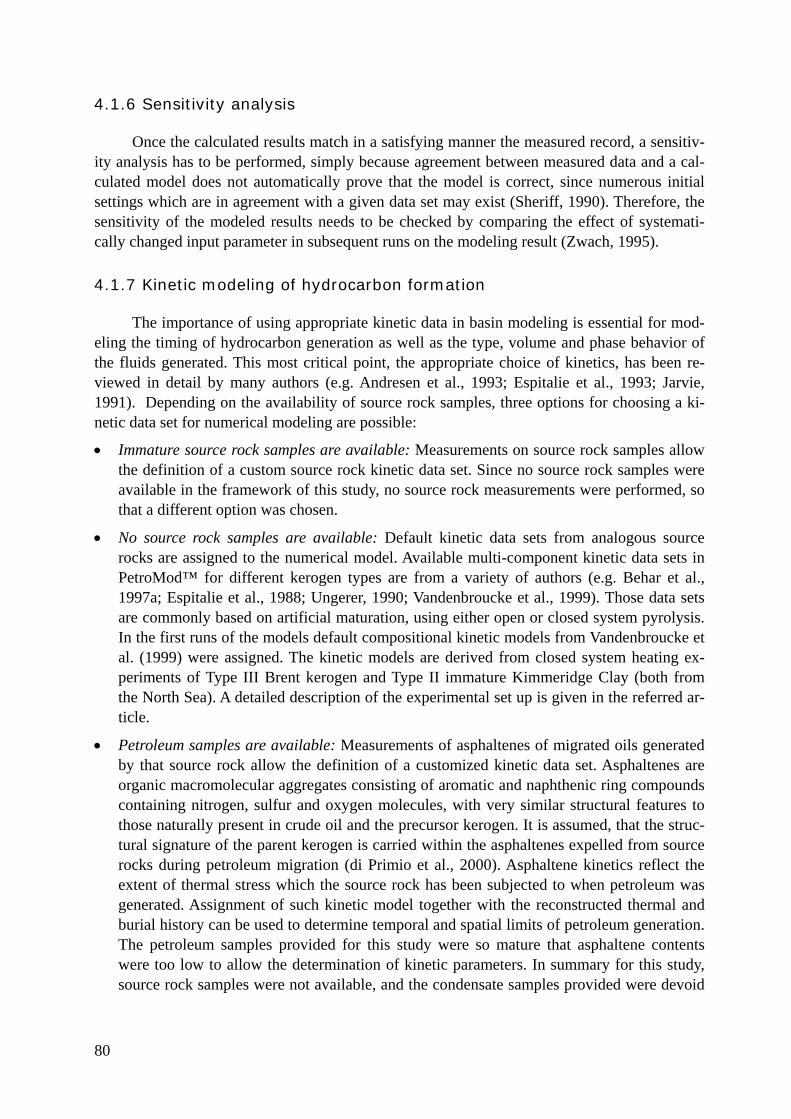
80

4.1.6 Sensitivity analysis

Once the calculated results match in a satisfying manner the measured record, a sensitiv-ity analysis has to be performed, simply because agreement between measured data and a cal-culated model does not automatically prove that the model is correct, since numerous initial settings which are in agreement with a given data set may exist (Sheriff, 1990). Therefore, the sensitivity of the modeled results needs to be checked by comparing the effect of systemati-cally changed input parameter in subsequent runs on the modeling result (Zwach, 1995).

4.1.7 Kinetic modeling of hydrocarbon formation

The importance of using appropriate kinetic data in basin modeling is essential for mod-eling the timing of hydrocarbon generation as well as the type, volume and phase behavior of the fluids generated. This most critical point, the appropriate choice of kinetics, has been re-viewed in detail by many authors (e.g. Andresen et al., 1993; Espitalie et al., 1993; Jarvie, 1991). Depending on the availability of source rock samples, three options for choosing a ki-netic data set for numerical modeling are possible:

• Immature source rock samples are available: Measurements on source rock samples allow the definition of a custom source rock kinetic data set. Since no source rock samples were available in the framework of this study, no source rock measurements were performed, so that a different option was chosen.

• No source rock samples are available: Default kinetic data sets from analogous source rocks are assigned to the numerical model. Available multi-component kinetic data sets in PetroMod™ for different kerogen types are from a variety of authors (e.g. Behar et al., 1997a; Espitalie et al., 1988; Ungerer, 1990; Vandenbroucke et al., 1999). Those data sets are commonly based on artificial maturation, using either open or closed system pyrolysis. In the first runs of the models default compositional kinetic models from Vandenbroucke et al. (1999) were assigned. The kinetic models are derived from closed system heating ex-periments of Type III Brent kerogen and Type II immature Kimmeridge Clay (both from the North Sea). A detailed description of the experimental set up is given in the referred ar-ticle.

• Petroleum samples are available: Measurements of asphaltenes of migrated oils generated by that source rock allow the definition of a customized kinetic data set. Asphaltenes are organic macromolecular aggregates consisting of aromatic and naphthenic ring compounds containing nitrogen, sulfur and oxygen molecules, with very similar structural features to those naturally present in crude oil and the precursor kerogen. It is assumed, that the struc-tural signature of the parent kerogen is carried within the asphaltenes expelled from source rocks during petroleum migration (di Primio et al., 2000). Asphaltene kinetics reflect the extent of thermal stress which the source rock has been subjected to when petroleum was generated. Assignment of such kinetic model together with the reconstructed thermal and burial history can be used to determine temporal and spatial limits of petroleum generation. The petroleum samples provided for this study were so mature that asphaltene contents were too low to allow the determination of kinetic parameters. In summary for this study, source rock samples were not available, and the condensate samples provided were devoid

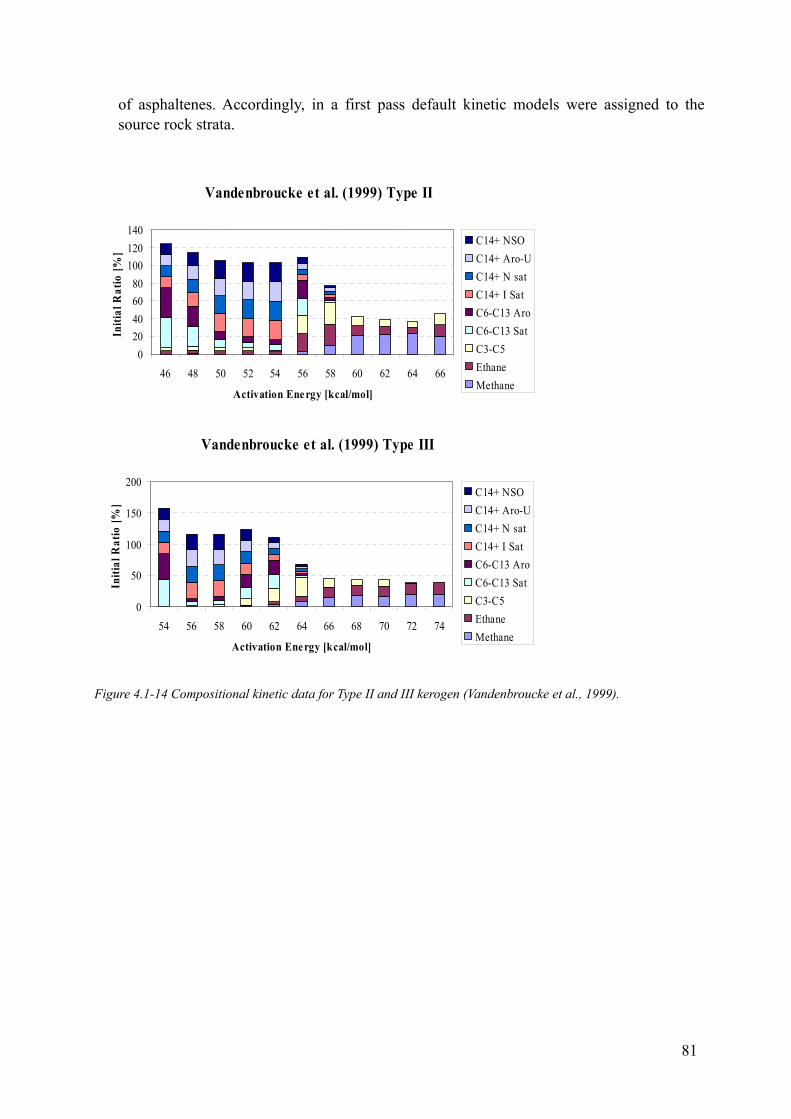
of asphaltenes. Accordingly, in a first pass default kinetic models were assigned to the source rock strata.

Vandenbroucke et al. (1999) Type II

020406080

100120140

46 48 50 52 54 56 58 60 62 64 66

Activation Ene rgy [kcal/mol]

Initi

al R

atio

[%]

C14+ NSOC14+ Aro-UC14+ N satC14+ I SatC6-C13 AroC6-C13 SatC3-C5EthaneMethane

Vandenbroucke et al. (1999) Type III

0

50

100

150

200

54 56 58 60 62 64 66 68 70 72 74

Activation Energy [kcal/mol]

Initi

al R

atio

[%]

C14+ NSOC14+ Aro-UC14+ N satC14+ I SatC6-C13 AroC6-C13 SatC3-C5EthaneMethane

Vandenbroucke et al. (1999) Type II

020406080

100120140

46 48 50 52 54 56 58 60 62 64 66

Activation Ene rgy [kcal/mol]

Initi

al R

atio

[%]

C14+ NSOC14+ Aro-UC14+ N satC14+ I SatC6-C13 AroC6-C13 SatC3-C5EthaneMethane

Vandenbroucke et al. (1999) Type III

0

50

100

150

200

54 56 58 60 62 64 66 68 70 72 74

Activation Energy [kcal/mol]

Initi

al R

atio

[%]

C14+ NSOC14+ Aro-UC14+ N satC14+ I SatC6-C13 AroC6-C13 SatC3-C5EthaneMethane

Figure 4.1-14 Compositional kinetic data for Type II and III kerogen (Vandenbroucke et al., 1999).

81

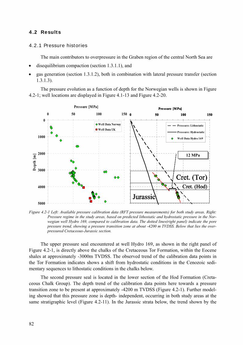
4.2 Results

4.2.1 Pressure histories

The main contributors to overpressure in the Graben region of the central North Sea are

• disequilibrium compaction (section 1.3.1.1), and

• gas generation (section 1.3.1.2), both in combination with lateral pressure transfer (section 1.3.1.3).

The pressure evolution as a function of depth for the Norwegian wells is shown in Figure 4.2-1; well locations are displayed in Figure 4.1-13 and Figure 4.2-20.

Cret. (Tor)

JurassicCret. (Hod)

0

1000

2000

3000

4000

5000

0 50 100 150

Pre ssure [M Pa]

Dep

th [m

]

Pressure: Lithostatic

Pressure: Hydrostatic

Well Data Hydro 169

12 MPa12 MPa

0

1000

2000

3000

4000

5000

0 50 100 150

Pressure [MPa]

Dep

th [m

]

Well Data NorwayWell Data UK

Cret. (Tor)

JurassicCret. (Hod)

0

1000

2000

3000

4000

5000

0 50 100 150

Pre ssure [M Pa]

Dep

th [m

]

Pressure: Lithostatic

Pressure: Hydrostatic

Well Data Hydro 169

12 MPa12 MPa

Cret. (Tor)

Jurassic

Cret. (Tor)

JurassicCret. (Hod)

0

1000

2000

3000

4000

5000

0 50 100 150

Pre ssure [M Pa]

Dep

th [m

]

Pressure: Lithostatic

Pressure: Hydrostatic

Well Data Hydro 169

12 MPa12 MPa

0

1000

2000

3000

4000

5000

0 50 100 150

Pressure [MPa]

Dep

th [m

]

Well Data NorwayWell Data UK

Figure 4.2-1 Left: Available pressure calibration data (RFT pressure measurements) for both study areas. Right: Pressure regime in the study areas, based on predicted lithostatic and hydrostatic pressure in the Nor-wegian well Hydro 169, compared to calibration data. The dotted lines(right panel) indicate the pore pressure trend, showing a pressure transition zone at about -4200 m TVDSS. Below that lies the over-pressured Cretaceous-Jurassic section.

The upper pressure seal encountered at well Hydro 169, as shown in the right panel of Figure 4.2-1, is directly above the chalks of the Cretaceous Tor Formation, within the Eocene shales at approximately -3000m TVDSS. The observed trend of the calibration data points in the Tor Formation indicates shows a shift from hydrostatic conditions in the Cenozoic sedi-mentary sequences to lithostatic conditions in the chalks below.

The second pressure seal is located in the lower section of the Hod Formation (Creta-ceous Chalk Group). The depth trend of the calibration data points here towards a pressure transition zone to be present at approximately -4200 m TVDSS (Figure 4.2-1). Further model-ing showed that this pressure zone is depth- independent, occurring in both study areas at the same stratigraphic level (Figure 4.2-11). In the Jurassic strata below, the trend shown by the

82

83

calibration data indicates a switch of the pressure regime at that depth back to hydrostatic con-ditions.

A variety of approaches to reproduce the pressure regimes in basin modeling are de-scribed in the literature (section 1.3.1). For any successful simulation, the effects of changing spatial or numerical model resolution or boundary conditions must be addressed. The following parameters were tested in detail during simulation:

• Changing the model’s scaling (maximum cell thickness, maximum time step duration, number of migration steps per time step) has no significant effects on the pressure-calculation, but it results in longer simulation times.

• It is not necessary to close the borders of the models; overpressure is retained even in open-bordered 3D modeling, while the generated hydrocarbons can leave the system through the sides.

• The Simulator/Options code “Oite 1000” increases the number of iterations in each time step (to e.g. 1000 in this case) and can be used to refine pressure modeling, but it results in an exponential increase in simulation times.

Indeed, changes applied to the options above may introduce some additional overpres-sure; however, its magnitude is not sufficient to seriously compromise the quality of the pres-sure calibration. Since overpressure in the North Sea Central Graben is commonly attributed to both, disequilibrium compaction as a function of the seal’s integrity and gas generation, the ef-fects of both mechanisms were tested in the models.

4.2.1.1 Seal Properties

A broad range of compaction-depth trends has been published. Those trends depend, in summary, on the initial porosity, the composition of the sediments and their age, the pressure regime and the temperature gradient (Giles et al., 1998). Overpressured areas show often po-rosities higher than the average. The effects of differential compacting of sediments were dis-cussed already in the nineteen twenties, for example by Monnett (1922), and also laboratory methods for determining parameters like bulk density and porosity were established already in the same period, for example by Athy (1930b), who described an exponential porosity-depth relationship based on 200 samples from Oklahoma shales (Equation 8):

Equation 8 z

oePP β−=

Po = average porosity β = compression parameterz = burial depth

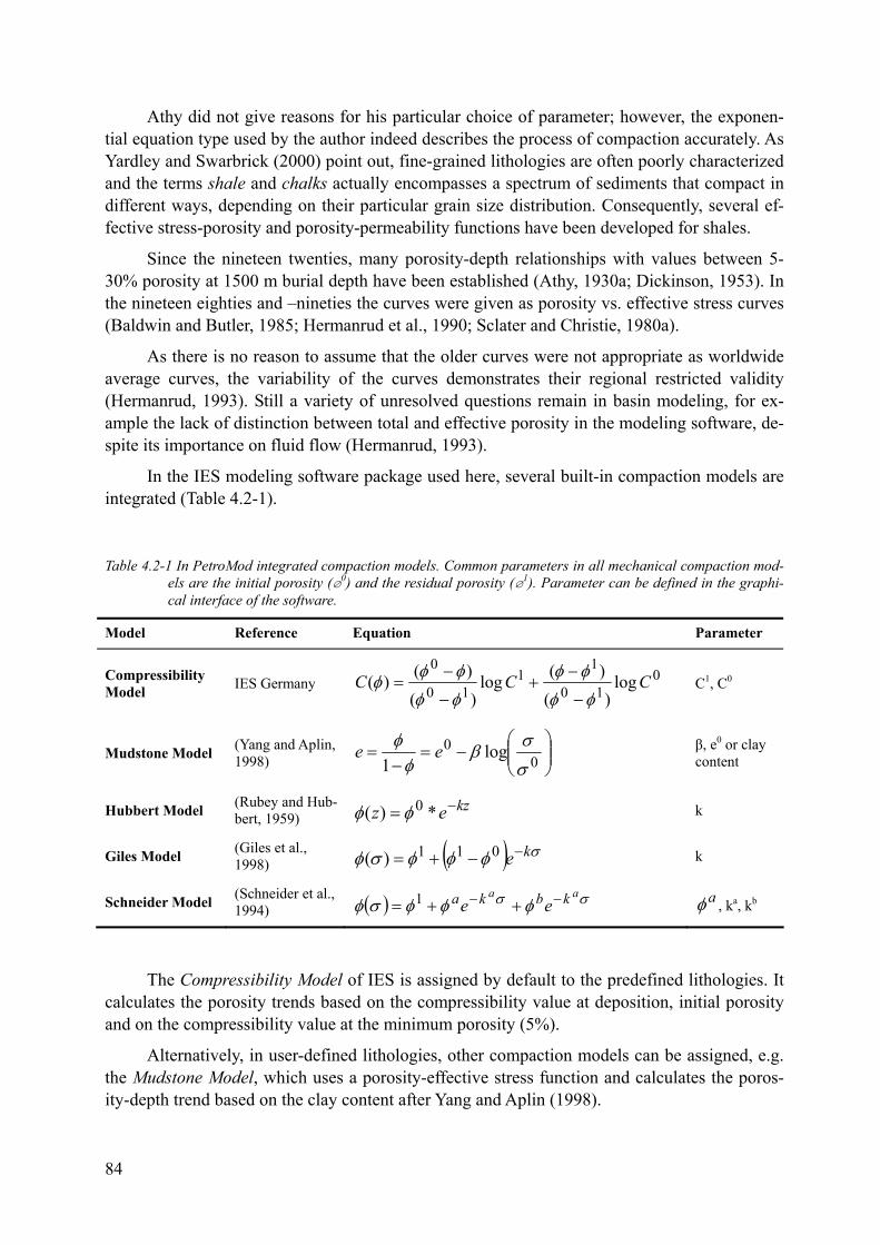
Athy did not give reasons for his particular choice of parameter; however, the exponen-tial equation type used by the author indeed describes the process of compaction accurately. As Yardley and Swarbrick (2000) point out, fine-grained lithologies are often poorly characterized and the terms shale and chalks actually encompasses a spectrum of sediments that compact in different ways, depending on their particular grain size distribution. Consequently, several ef-fective stress-porosity and porosity-permeability functions have been developed for shales.

Since the nineteen twenties, many porosity-depth relationships with values between 5-30% porosity at 1500 m burial depth have been established (Athy, 1930a; Dickinson, 1953). In the nineteen eighties and –nineties the curves were given as porosity vs. effective stress curves (Baldwin and Butler, 1985; Hermanrud et al., 1990; Sclater and Christie, 1980a).

As there is no reason to assume that the older curves were not appropriate as worldwide average curves, the variability of the curves demonstrates their regional restricted validity (Hermanrud, 1993). Still a variety of unresolved questions remain in basin modeling, for ex-ample the lack of distinction between total and effective porosity in the modeling software, de-spite its importance on fluid flow (Hermanrud, 1993).

In the IES modeling software package used here, several built-in compaction models are integrated (Table 4.2-1).

Table 4.2-1 In PetroMod integrated compaction models. Common parameters in all mechanical compaction mod-els are the initial porosity (i0) and the residual porosity (i1). Parameter can be defined in the graphi-cal interface of the software.

Model Reference Equation Parameter

010

11

10

0log

)()(log

)()()( CCC

φφ

φφ

φφ

φφφ−

−+

−

−=Compressibility

Model IES Germany C1, C0

⎟⎟⎠

⎞⎜⎜⎝

⎛−=

−= 0

0 log1 σ

σβφ

φ ee β, e0 or clay content

(Yang and Aplin, 1998) Mudstone Model

(Rubey and Hub-bert, 1959)

kzez −= *)( 0φφHubbert Model k

( ) σφφφσφ ke−−+= 011)((Giles et al., 1998) Giles Model k

(Schneider et al., 1994) ( ) σσ φφφσφ

aa kbka ee −− ++= 1 aφSchneider Model , ka, kb

Compressibility ModelThe of IES is assigned by default to the predefined lithologies. It calculates the porosity trends based on the compressibility value at deposition, initial porosity and on the compressibility value at the minimum porosity (5%).

Alternatively, in user-defined lithologies, other compaction models can be assigned, e.g. the Mudstone Model, which uses a porosity-effective stress function and calculates the poros-ity-depth trend based on the clay content after Yang and Aplin (1998).

84

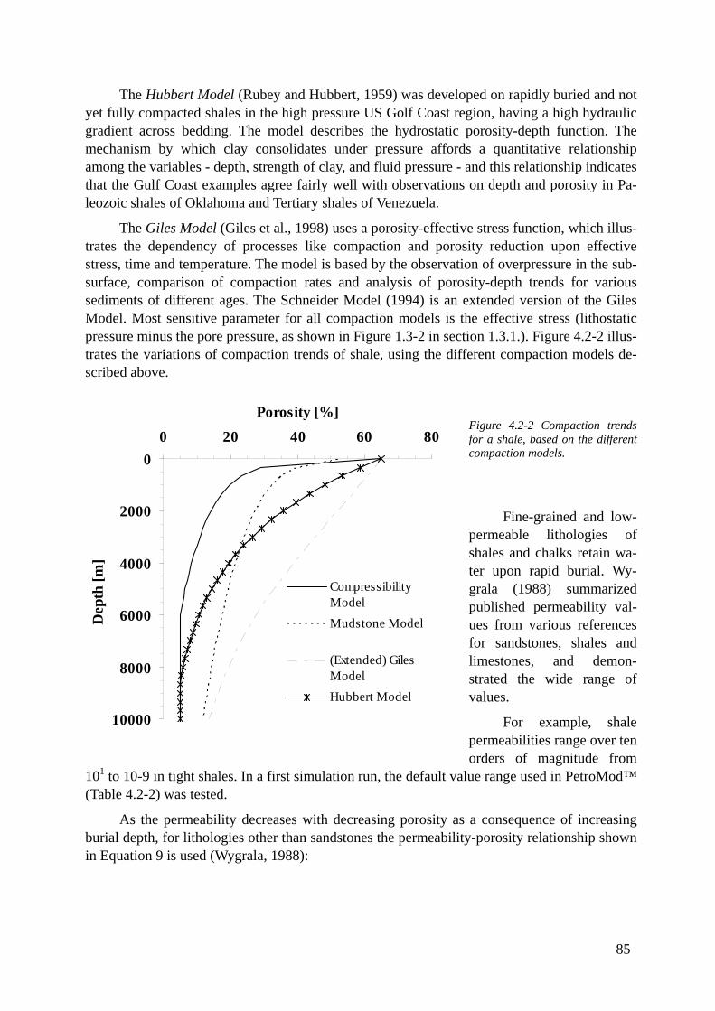
85

The Hubbert Model (Rubey and Hubbert, 1959) was developed on rapidly buried and not yet fully compacted shales in the high pressure US Golf Coast region, having a high hydraulic gradient across bedding. The model describes the hydrostatic porosity-depth function. The mechanism by which clay consolidates under pressure affords a quantitative relationship among the variables - depth, strength of clay, and fluid pressure - and this relationship indicates that the Gulf Coast examples agree fairly well with observations on depth and porosity in Pa-leozoic shales of Oklahoma and Tertiary shales of Venezuela.

The Giles Model (Giles et al., 1998) uses a porosity-effective stress function, which illus-trates the dependency of processes like compaction and porosity reduction upon effective stress, time and temperature. The model is based by the observation of overpressure in the sub-surface, comparison of compaction rates and analysis of porosity-depth trends for various sediments of different ages. The Schneider Model (1994) is an extended version of the Giles Model. Most sensitive parameter for all compaction models is the effective stress (lithostatic pressure minus the pore pressure, as shown in Figure 1.3-2 in section 1.3.1.). Figure 4.2-2 illus-trates the variations of compaction trends of shale, using the different compaction models de-scribed above.

Figure 4.2-2 Compaction trends for a shale, based on the different compaction models.

Fine-grained and low-permeable lithologies of shales and chalks retain wa-ter upon rapid burial. Wy-grala (1988) summarized published permeability val-ues from various references for sandstones, shales and limestones, and demon-strated the wide range of values.

For example, shale permeabilities range over ten orders of magnitude from

101 to 10-9 in tight shales. In a first simulation run, the default value range used in PetroMod™ (Table 4.2-2) was tested.

As the permeability decreases with decreasing porosity as a consequence of increasing burial depth, for lithologies other than sandstones the permeability-porosity relationship shown in Equation 9 is used (Wygrala, 1988):

0

2000

4000

6000

8000

10000

0 20 40 60 80

Porosity [%]

Dep

th [m

]

CompressibilityModelMudstone Model

(Extended) GilesModelHubbert Model

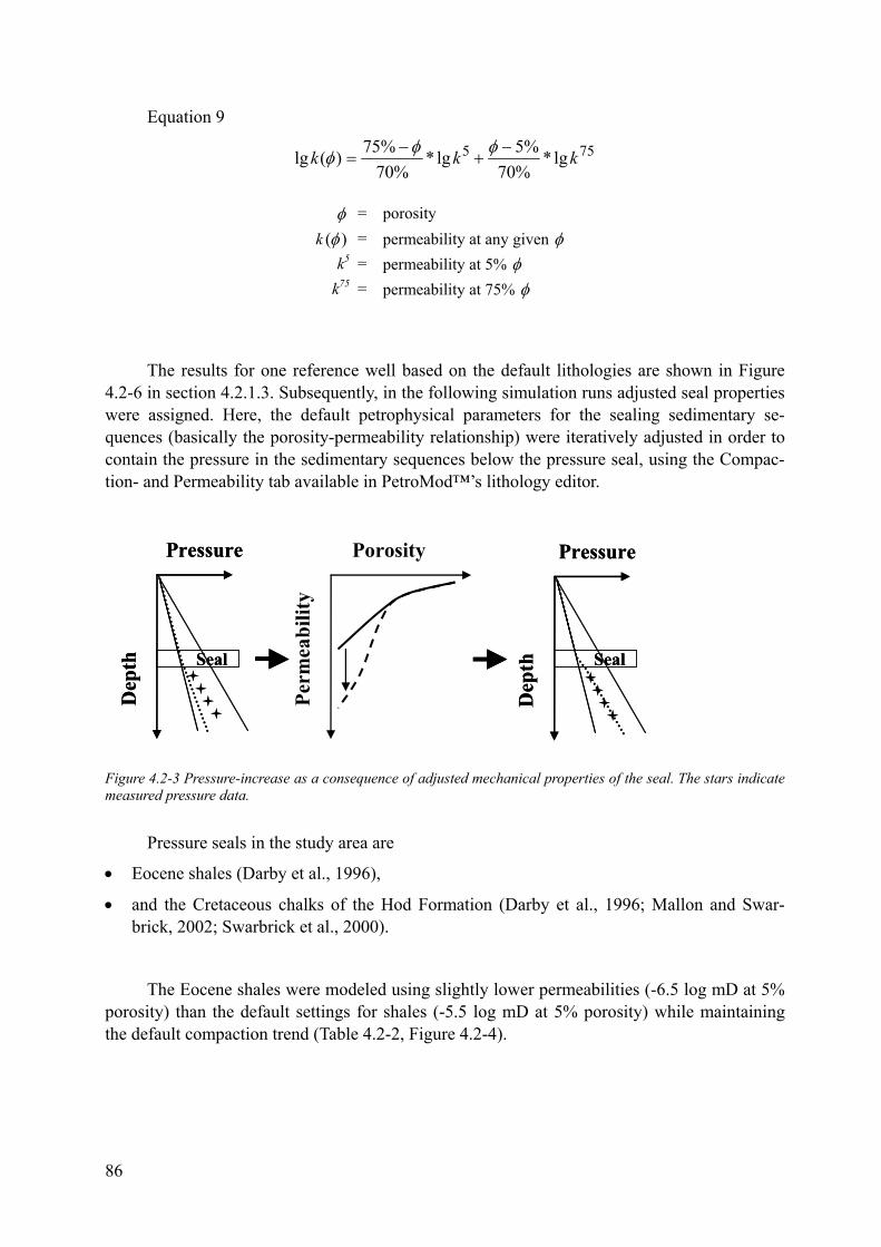
Equation 9

755 lg*%70%5lg*

%70%75)(lg kkk −

+−

=φφφ

φ = porosity )(φk = permeability at any given φ k5 = permeability at 5% φ

k75 = permeability at 75% φ

The results for one reference well based on the default lithologies are shown in Figure 4.2-6 in section 4.2.1.3. Subsequently, in the following simulation runs adjusted seal properties were assigned. Here, the default petrophysical parameters for the sealing sedimentary se-quences (basically the porosity-permeability relationship) were iteratively adjusted in order to contain the pressure in the sedimentary sequences below the pressure seal, using the Compac-tion- and Permeability tab available in PetroMod™’s lithology editor.

SealSeal

Pressure

Dep

th

PressureD

epth

Porosity

Perm

eabi

lity

SealSeal

Pressure

Dep

th

PressureD

epth

Porosity

Perm

eabi

lity

Figure 4.2-3 Pressure-increase as a consequence of adjusted mechanical properties of the seal. The stars indicate measured pressure data.

Pressure seals in the study area are

• Eocene shales (Darby et al., 1996),

• and the Cretaceous chalks of the Hod Formation (Darby et al., 1996; Mallon and Swar-brick, 2002; Swarbrick et al., 2000).

The Eocene shales were modeled using slightly lower permeabilities (-6.5 log mD at 5% porosity) than the default settings for shales (-5.5 log mD at 5% porosity) while maintaining the default compaction trend (Table 4.2-2, Figure 4.2-4).

86

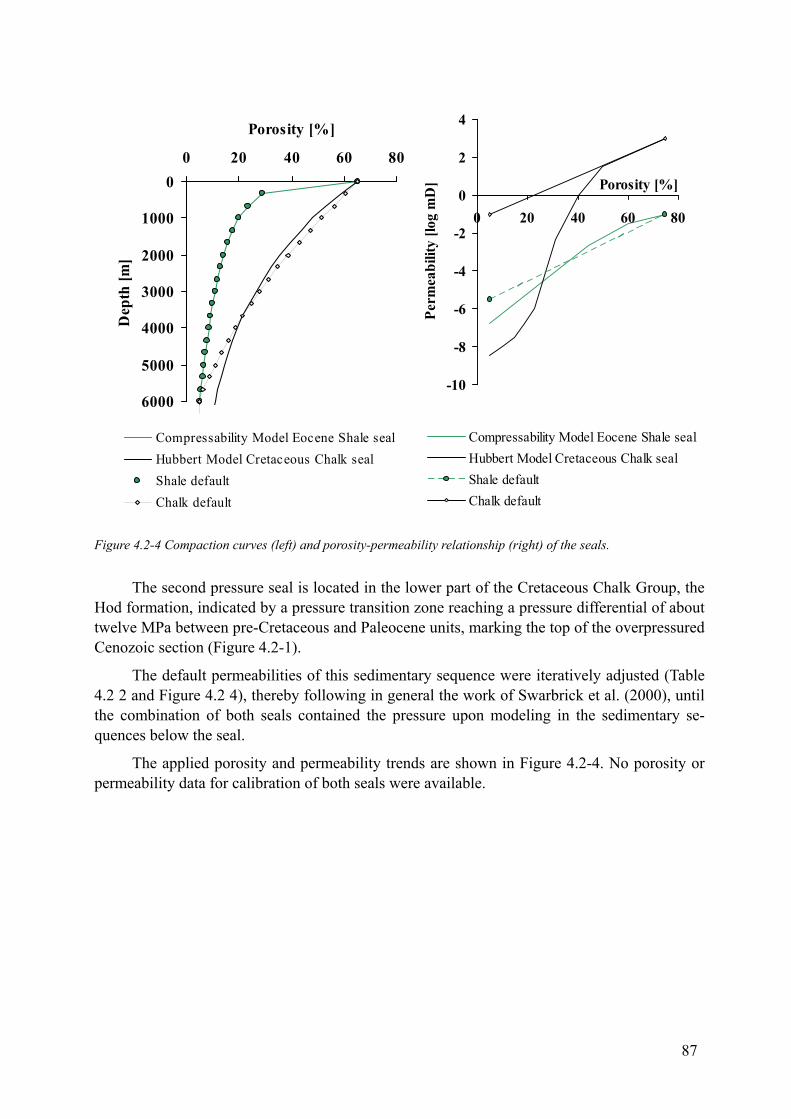
0

1000

2000

3000

4000

5000

6000

0 20 40 60 80

Porosity [%]D

epth

[m]

Compressability Model Eocene Shale sealHubbert Model Cretaceous Chalk sealShale defaultChalk default

-10

-8

-6

-4

-2

0

2

4

0 20 40 60 80

Porosity [%]

Perm

eabi

lity

[log

mD

]Compressability Model Eocene Shale sealHubbert Model Cretaceous Chalk sealShale defaultChalk default

0

1000

2000

3000

4000

5000

6000

0 20 40 60 80

Porosity [%]D

epth

[m]

Compressability Model Eocene Shale sealHubbert Model Cretaceous Chalk sealShale defaultChalk default

-10

-8

-6

-4

-2

0

2

4

0 20 40 60 80

Porosity [%]

Perm

eabi

lity

[log

mD

]Compressability Model Eocene Shale sealHubbert Model Cretaceous Chalk sealShale defaultChalk default

Figure 4.2-4 Compaction curves (left) and porosity-permeability relationship (right) of the seals.

The second pressure seal is located in the lower part of the Cretaceous Chalk Group, the Hod formation, indicated by a pressure transition zone reaching a pressure differential of about twelve MPa between pre-Cretaceous and Paleocene units, marking the top of the overpressured Cenozoic section (Figure 4.2-1).

The default permeabilities of this sedimentary sequence were iteratively adjusted (Table 4.2 2 and Figure 4.2 4), thereby following in general the work of Swarbrick et al. (2000), until the combination of both seals contained the pressure upon modeling in the sedimentary se-quences below the seal.

The applied porosity and permeability trends are shown in Figure 4.2-4. No porosity or permeability data for calibration of both seals were available.

87

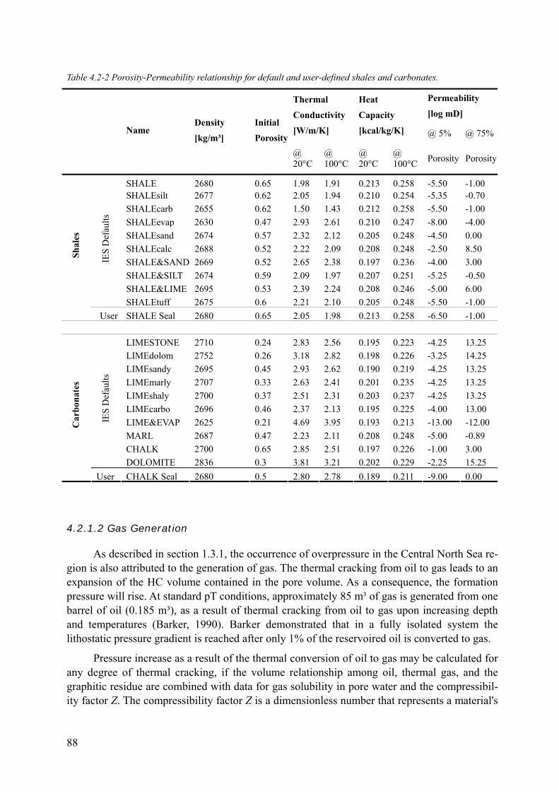
Table 4.2-2 Porosity-Permeability relationship for default and user-defined shales and carbonates.

Permeability Thermal Heat [log mD] Conductivity Capacity

[W/m/K] [kcal/kg/K] @ 5% @ 75% Name Density Initial

Porosity[kg/m³] @ 20°C

@ 100°C

@ 20°C

@ 100°C Porosity Porosity

SHALE 2680 0.65 1.98 1.91 0.213 0.258 -5.50 -1.00SHALEsilt 2677 0.62 2.05 1.94 0.210 0.254 -5.35 -0.70SHALEcarb 2655 0.62 1.50 1.43 0.212 0.258 -5.50 -1.00

IES

Def

aults

SHALEevap 2630 0.47 2.93 2.61 0.210 0.247 -8.00 -4.00SHALEsand 2674 0.57 2.32 2.12 0.205 0.248 -4.50 0.00

Shal

es

SHALEcalc 2688 0.52 2.22 2.09 0.208 0.248 -2.50 8.50SHALE&SAND 2669 0.52 2.65 2.38 0.197 0.236 -4.00 3.00SHALE&SILT 2674 0.59 2.09 1.97 0.207 0.251 -5.25 -0.50SHALE&LIME 2695 0.53 2.39 2.24 0.208 0.246 -5.00 6.00SHALEtuff 2675 0.6 2.21 2.10 0.205 0.248 -5.50 -1.00

User SHALE Seal 2680 0.65 2.05 1.98 0.213 0.258 -6.50 -1.00

LIMESTONE 2710 0.24 2.83 2.56 0.195 0.223 -4.25 13.25LIMEdolom 2752 0.26 3.18 2.82 0.198 0.226 -3.25 14.25LIMEsandy 2695 0.45 2.93 2.62 0.190 0.219 -4.25 13.25

IES

Def

aults

LIMEmarly 2707 0.33 2.63 2.41 0.201 0.235 -4.25 13.25

Car

bona

tes

LIMEshaly 2700 0.37 2.51 2.31 0.203 0.237 -4.25 13.25LIMEcarbo 2696 0.46 2.37 2.13 0.195 0.225 -4.00 13.00LIME&EVAP 2625 0.21 4.69 3.95 0.193 0.213 -13.00 -12.00MARL 2687 0.47 2.23 2.11 0.208 0.248 -5.00 -0.89CHALK 2700 0.65 2.85 2.51 0.197 0.226 -1.00 3.00DOLOMITE 2836 0.3 3.81 3.21 0.202 0.229 -2.25 15.25

User CHALK Seal 2680 0.5 2.80 2.78 0.189 0.211 -9.00 0.00

4.2.1.2 Gas Generation

As described in section 1.3.1, the occurrence of overpressure in the Central North Sea re-gion is also attributed to the generation of gas. The thermal cracking from oil to gas leads to an expansion of the HC volume contained in the pore volume. As a consequence, the formation pressure will rise. At standard pT conditions, approximately 85 m³ of gas is generated from one barrel of oil (0.185 m³), as a result of thermal cracking from oil to gas upon increasing depth and temperatures (Barker, 1990). Barker demonstrated that in a fully isolated system the lithostatic pressure gradient is reached after only 1% of the reservoired oil is converted to gas.

Pressure increase as a result of the thermal conversion of oil to gas may be calculated for any degree of thermal cracking, if the volume relationship among oil, thermal gas, and the graphitic residue are combined with data for gas solubility in pore water and the compressibil-ity factor Z. The compressibility factor Z is a dimensionless number that represents a material's

88

deviation from ideal gas behavior described by Boyle’s and Charles' laws. For lower pressures and small non-polar molecules an assumed compressibility factor value of 1 is a good first guess. At higher pressures and with larger molecular weight of polar molecules the compressi-bility factor will fall below 1. Z is defined as (Equation 10):

RTpVZ =

p = pressure T = temperature R = gas constant V = molar volume of the gas

For an ideal gas, Z is 1; in a real gas, Z is either below or above 1. Z can also be deter-mined graphically, using the generalized compressibility factor chart (Figure 4.2-5), which was first introduced by (Nelson and Obert, 1954).

The chart shows reduced temperature (Tr) trends between 1.0 and 15 for a reduced pres-sure (P ) range between Pr r = 0 to 30 for methane. To use that chart, reduced and critical values for temperature and pressure of the specific substance need to be determined.

On diagrams showing the thermodynamic properties for a given substance, the point at critical temperature and critical pressure is called the critical point of the substance. Above its critical temperature, a gas cannot be liquefied.

The critical temperature (Tcr) is defined as that point, above which no distinction be-tween liquid and gas phase can be made, because the physical properties of both phases be-come equal. The critical pressure (Pcr) is the vapor pressure at the critical temperature. An ex-ample for a PT phase diagram for a multicomponent fluid which includes the critical point for the specific substance is shown in Figure 1.2-2.

11:

In thermodynamics, T and Pr r use the specific critical point as the basis of comparison by dividing the actual state variable (T, P) by its critical equivalent (T , Pcr cr); they represent ratios of the reservoir conditions and the fluids critical conditions. T and P are dimensionless. Tr r r and P were calculated, using the following Equation r

crr P

PP =cr

r TTT =

and

To obtain Z, P was plotted versus Tr r. Data input were the values of the pressure (851.5 bar) and temperature (190.7°C) conditions encountered in the Jade DST 1, as shown in the box integrated in Figure 4.2-5. Z can than be read directly at the y-axis.

89

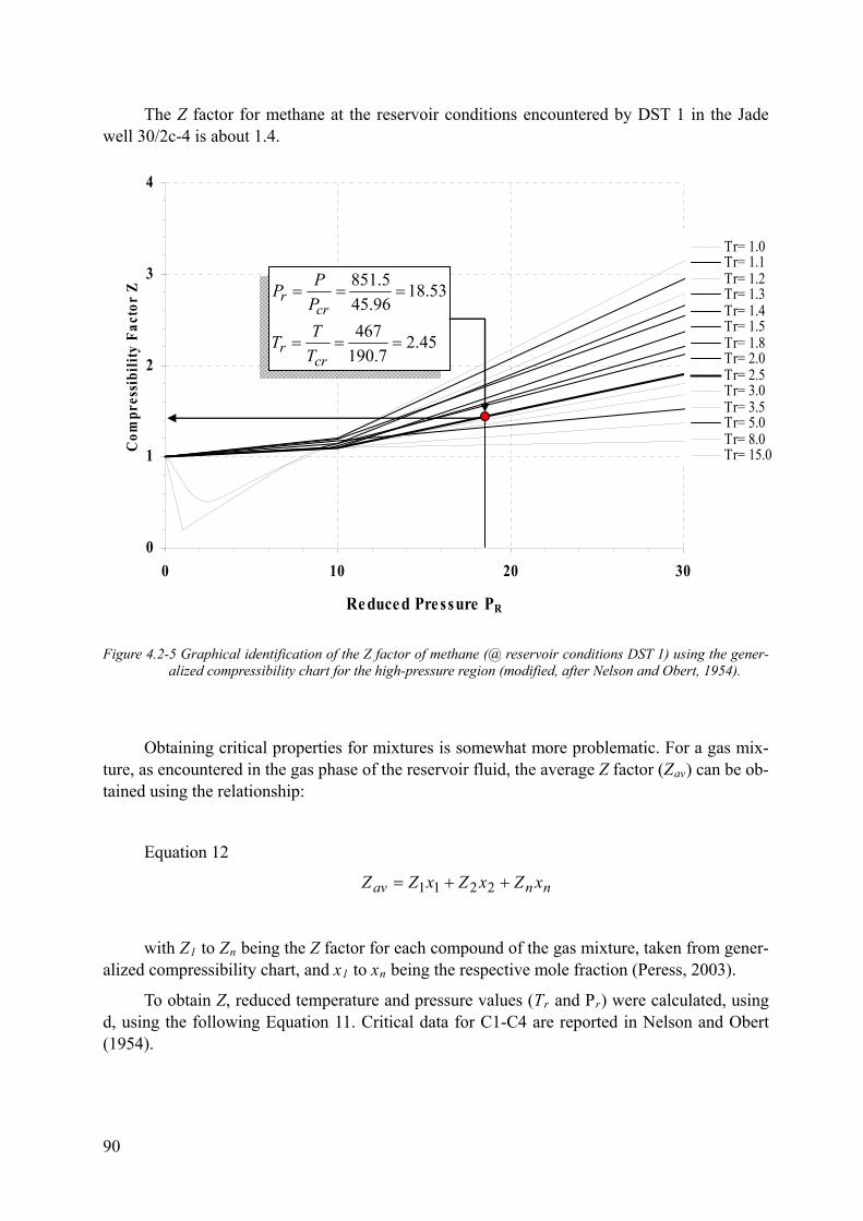
The Z factor for methane at the reservoir conditions encountered by DST 1 in the Jade well 30/2c-4 is about 1.4.

0

1

2

3

4

0 10 20 30

Re duced Pre ssure PR

Com

pres

sibi

lity

Fact

or Z

Tr= 1.0Tr= 1.1Tr= 1.2Tr= 1.3Tr= 1.4Tr= 1.5Tr= 1.8Tr= 2.0Tr= 2.5Tr= 3.0Tr= 3.5Tr= 5.0Tr= 8.0Tr= 15.0

45.27.190

467

53.1845.96851.5

===

===

crr

crr

TTT

PPP

0

1

2

3

4

0 10 20 30

Re duced Pre ssure PR

Com

pres

sibi

lity

Fact

or Z

Tr= 1.0Tr= 1.1Tr= 1.2Tr= 1.3Tr= 1.4Tr= 1.5Tr= 1.8Tr= 2.0Tr= 2.5Tr= 3.0Tr= 3.5Tr= 5.0Tr= 8.0Tr= 15.0

45.27.190

467

53.1845.96851.5

===

===

crr

crr

TTT

PPP

Figure 4.2-5 Graphical identification of the Z factor of methane (@ reservoir conditions DST 1) using the gener-alized compressibility chart for the high-pressure region (modified, after Nelson and Obert, 1954).

Obtaining critical properties for mixtures is somewhat more problematic. For a gas mix-ture, as encountered in the gas phase of the reservoir fluid, the average Z factor (Zav) can be ob-tained using the relationship:

Equation 12

nnav xZxZxZZ ++= 2211

with Z to Z1 n being the Z factor for each compound of the gas mixture, taken from gener-alized compressibility chart, and x to x being the respective mole fraction (Peress, 2003). 1 n

To obtain Z, reduced temperature and pressure values (T and P ) were calculated, using r r

d, using the following Equation 11. Critical data for C1-C4 are reported in Nelson and Obert (1954).

90

Table 4.2-3 Critical data and Z factors for the C1-nC4 fraction of the gas condensate tested in the deeper DST 1 of the Jade well 30/2c-4.

Respective Mole frac-tion

Critical Data Reduced Values Z (Generalized Compound

T [°C/K] P [bar] T P Compress. Chart) critical critical reduced reduced

C1 0.71883 -82.7/190 45.96 2.45 18.53 1.4

C2 0.08299 32.2/305 48.84 1.53 17.43 1.6

C3 0.03520 96.6/369 42.5 1.27 20.04 1.8

iC4 0.00820 134.9/408 36.48 1.14 23.34 2.2

nC4 0.01350 190.5/464 46 1.01 18.51 2.0

T [°C/K]: P [bar]: Reservoir Conditions Z average 1.247546

193.89/467 851.5

The thus obtained average Z factor of 1.25 (Table 4.2-3) is confirmed by the Z factor cal-culated with the PVT-modeling software PVTsim Vs. 13.1 (Calsep, A/S, Denmark), which solves Z to be 1.2 (Table 4.2-4).

Table 4.2-4 Calculated phase properties and Z factor of the reservoir fluid (DST 1 Jade 30/2c-4, UK), using PVT modeling software (PVTsim 13.1).

To determine the extent of pressure generation solely by gas generation, default lithologies were assigned to the pressure seals (Eo-cene: shales; Cretaceous: chalks), and the determined Z factor of the multicomponent reservoir fluid (Ta-ble 4.2-4) was integrated into the numerical models using the follow-

ing code in the Simulation/Options tab of the PetroMod™ Simulation tool. To define the code, the reciprocal of the compressibility (Z) of gas is used, because it is the equivalent of the coef-ficient of elasticity, the latter being the more commonly used term in physics and mechanics:

Phase Properties @ 432.06 bar and 68.93°C (CriticalPoint)

Volume cm³/mol 79.6

Density g/cm³ 0.4726

Z Factor 1.2091

Molecular Weight 37.62

Oela 833, 833 being the reciprocal of Z of gas, expressed in MPa:

1200 MPa = 1.2 GPa (1/Z = 1/1.2 GPa = 0.833 GPa-1).

The results of both approaches, of the modified petrophysical properties of the sealing formations and overpressure generation by gas generation, are shown in the following section.

91

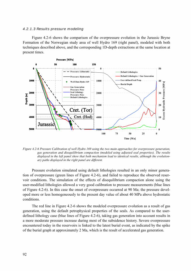
4.2.1.3 Results pressure modeling

Figure 4.2-6 shows the comparison of the overpressure evolution in the Jurassic Bryne Formation of the Norwegian study area of well Hydro 169 (right panel), modeled with both techniques described above, and the corresponding 1D-depth extractions at the same location at present times.

0

10

20

30

40

50

0255075100

Time [M a]

Exc

ess H

ydra

ulic

Pre

ssur

e [M

Pa]

0

1000

2000

3000

4000

5000

Default Lithologies

Default Lithologies + Gas Generation

User defined Seal Prop.

Burial Depth

Cret. (Tor)

JurassicCret. (Hod)

0

1000

2000

3000

4000

5000

0 50 100 150

Pressure [MPa]

Dep

th [m

]

Pressure: Lithostatic

Pressure: Hydrostatic

Well Data Hydro 169

Gas GenerationPressure: PoreSeal LithologyPressure: PoreDefault Lithologies

0

10

20

30

40

50

0255075100

Time [M a]

Exc

ess H

ydra

ulic

Pre

ssur

e [M

Pa]

0

1000

2000

3000

4000

5000

Default Lithologies

Default Lithologies + Gas Generation

User defined Seal Prop.

Burial Depth

Cret. (Tor)

JurassicCret. (Hod)

0

1000

2000

3000

4000

5000

0 50 100 150

Pressure [MPa]

Dep

th [m

]

Pressure: Lithostatic

Pressure: Hydrostatic

Well Data Hydro 169

Gas GenerationPressure: PoreSeal LithologyPressure: PoreDefault Lithologies

Cret. (Tor)

Jurassic

Cret. (Tor)

JurassicCret. (Hod)

0

1000

2000

3000

4000

5000

0 50 100 150

Pressure [MPa]

Dep

th [m

]

Pressure: Lithostatic

Pressure: Hydrostatic

Well Data Hydro 169

Gas GenerationPressure: PoreSeal LithologyPressure: PoreDefault Lithologies

Figure 4.2-6 Pressure Calibration of well Hydro 169 using the two main approaches for overpressure generation, gas generation and disequilibrium compaction (modeled using adjusted seal properties). The results displayed in the left panel show that both mechanism lead to identical results, although the evolution-ary paths displayed in the right panel are different.

Pressure evolution simulated using default lithologies resulted in an only minor genera-tion of overpressure (green lines of Figure 4.2-6), and failed to reproduce the observed reser-voir conditions. The simulation of the effects of disequilibrium compaction alone using the user-modified lithologies allowed a very good calibration to pressure measurements (blue lines of Figure 4.2-6). In this case the onset of overpressure occurred at 90 Ma; the pressure devel-oped more or less homogeneously to the present day value of about 40 MPa above hydrostatic conditions.

The red line in Figure 4.2-6 shows the modeled overpressure evolution as a result of gas generation, using the default petrophysical properties of the seals. As compared to the user-defined lithology case (blue lines of Figure 4.2-6), taking gas generation into account results in a more moderate pressure increase during most of the subsidence history. Severe overpressure encountered today in the reservoirs is linked to the latest burial event, as indicated by the spike of the burial graph at approximately 2 Ma, which is the result of accelerated gas generation.

92

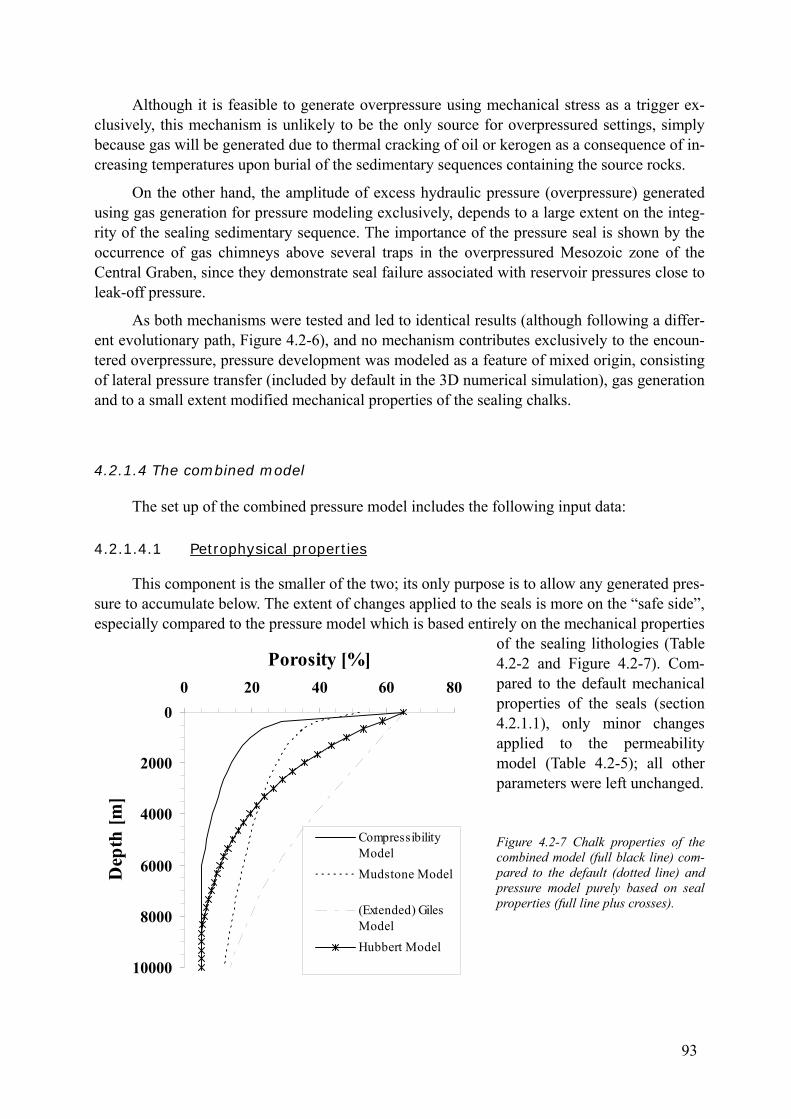
Although it is feasible to generate overpressure using mechanical stress as a trigger ex-clusively, this mechanism is unlikely to be the only source for overpressured settings, simply because gas will be generated due to thermal cracking of oil or kerogen as a consequence of in-creasing temperatures upon burial of the sedimentary sequences containing the source rocks.

On the other hand, the amplitude of excess hydraulic pressure (overpressure) generated using gas generation for pressure modeling exclusively, depends to a large extent on the integ-rity of the sealing sedimentary sequence. The importance of the pressure seal is shown by the occurrence of gas chimneys above several traps in the overpressured Mesozoic zone of the Central Graben, since they demonstrate seal failure associated with reservoir pressures close to leak-off pressure.

As both mechanisms were tested and led to identical results (although following a differ-ent evolutionary path, Figure 4.2-6), and no mechanism contributes exclusively to the encoun-tered overpressure, pressure development was modeled as a feature of mixed origin, consisting of lateral pressure transfer (included by default in the 3D numerical simulation), gas generation and to a small extent modified mechanical properties of the sealing chalks.

4.2.1.4 The combined model

The set up of the combined pressure model includes the following input data:

4.2.1.4.1 Petrophysical properties

This component is the smaller of the two; its only purpose is to allow any generated pres-sure to accumulate below. The extent of changes applied to the seals is more on the “safe side”, especially compared to the pressure model which is based entirely on the mechanical properties

of the sealing lithologies (Table 4.2-2 and Figure 4.2-7). Com-pared to the default mechanical properties of the seals (section 4.2.1.1), only minor changes applied to the permeability model (Table 4.2-5); all other parameters were left unchanged.

Figure 4.2-7 Chalk properties of the combined model (full black line) com-pared to the default (dotted line) and pressure model purely based on seal properties (full line plus crosses).

0

2000

4000

6000

8000

10000

0 20 40 60 80

Porosity [%]

Dep

th [m

]

CompressibilityModelMudstone Model

(Extended) GilesModelHubbert Model

93

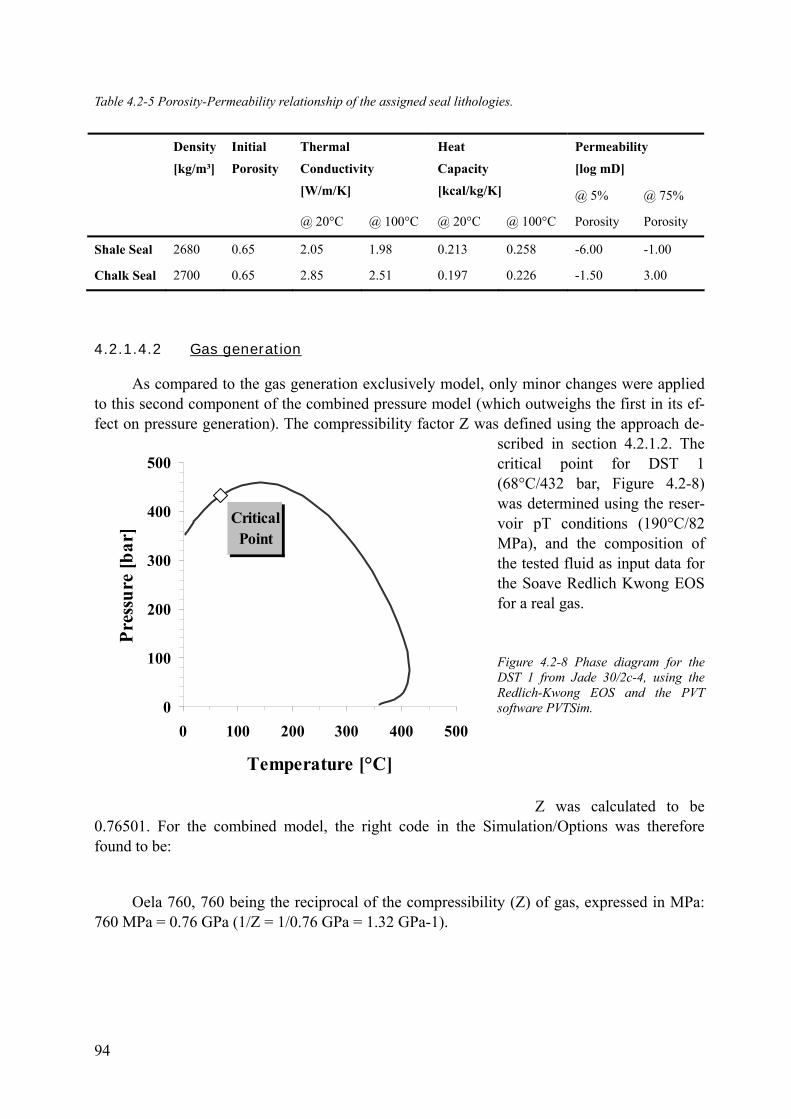
Table 4.2-5 Porosity-Permeability relationship of the assigned seal lithologies.

Density Initial Thermal Heat Permeability

[kg/m³] Porosity Conductivity Capacity [log mD]

[W/m/K] [kcal/kg/K] @ 5% @ 75%

@ 20°C @ 100°C @ 20°C @ 100°C Porosity Porosity

Shale Seal 2680 0.65 2.05 1.98 0.213 0.258 -6.00 -1.00

Chalk Seal 2700 0.65 2.85 2.51 0.197 0.226 -1.50 3.00

4.2.1.4.2 Gas generation

As compared to the gas generation exclusively model, only minor changes were applied to this second component of the combined pressure model (which outweighs the first in its ef-fect on pressure generation). The compressibility factor Z was defined using the approach de-

scribed in section 4.2.1.2. The critical point for DST 1 (68°C/432 bar,

Critical Point

0

100

200

300

400

500

0 100 200 300 400 500

Temperature [°C]

Pres

sure

[bar

]

Figure 4.2-8) was determined using the reser-voir pT conditions (190°C/82 MPa), and the composition of the tested fluid as input data for the Soave Redlich Kwong EOS for a real gas.

Figure 4.2-8 Phase diagram for the DST 1 from Jade 30/2c-4, using the Redlich-Kwong EOS and the PVT software PVTSim.

Z was calculated to be 0.76501. For the combined model, the right code in the Simulation/Options was therefore found to be:

Oela 760, 760 being the reciprocal of the compressibility (Z) of gas, expressed in MPa: 760 MPa = 0.76 GPa (1/Z = 1/0.76 GPa = 1.32 GPa-1).

94

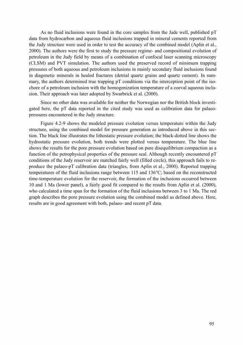
As no fluid inclusions were found in the core samples from the Jade well, published pT data from hydrocarbon and aqueous fluid inclusions trapped in mineral cements reported from the Judy structure were used in order to test the accuracy of the combined model (Aplin et al., 2000). The authors were the first to study the pressure regime- and compositional evolution of petroleum in the Judy field by means of a combination of confocal laser scanning microscopy (CLSM) and PVT simulation. The authors used the preserved record of minimum trapping pressures of both aqueous and petroleum inclusions in mainly secondary fluid inclusions found in diagenetic minerals in healed fractures (detrial quartz grains and quartz cement). In sum-mary, the authors determined true trapping pT conditions via the interception point of the iso-chore of a petroleum inclusion with the homogenization temperature of a coeval aqueous inclu-sion. Their approach was later adopted by Swarbrick et al. (2000).

Since no other data was available for neither the Norwegian nor the British block investi-gated here, the pT data reported in the cited study was used as calibration data for palaeo-pressures encountered in the Judy structure.

Figure 4.2-9 shows the modeled pressure evolution versus temperature within the Judy structure, using the combined model for pressure generation as introduced above in this sec-tion. The black line illustrates the lithostatic pressure evolution; the black-dotted line shows the hydrostatic pressure evolution, both trends were plotted versus temperature. The blue line shows the results for the pore pressure evolution based on pure disequilibrium compaction as a function of the petrophysical properties of the pressure seal. Although recently encountered pT conditions of the Judy reservoir are matched fairly well (filled circle), this approach fails to re-produce the palaeo-pT calibration data (triangles, from Aplin et al., 2000). Reported trapping temperatures of the fluid inclusions range between 115 and 136°C; based on the reconstructed time-temperature evolution for the reservoir, the formation of the inclusions occurred between 10 and 1 Ma (lower panel), a fairly good fit compared to the results from Aplin et al. (2000), who calculated a time span for the formation of the fluid inclusions between 3 to 1 Ma. The red graph describes the pore pressure evolution using the combined model as defined above. Here, results are in good agreement with both, palaeo- and recent pT data.

95

0

10

20

30

40

50

60

70

80

90

0 25 50 75 100 125 150

Pres

sure

[MPa

]Pressure: Lithostatic

Pressure: Hydrostatic

Pressure: Pore (Z=760)

Pressure: Pore (Seal Prop.)

Fluid Incl. (Aplin et al., 2000)

Judy pT reservoir cond.

0

50

100

150

200

0 25 50 75 100 125 150

Temperature [°C]

Tim

e [M

a]

Temperature

0

10

20

30

40

50

60

70

80

90

0 25 50 75 100 125 150

Pres

sure

[MPa

]Pressure: Lithostatic

Pressure: Hydrostatic

Pressure: Pore (Z=760)

Pressure: Pore (Seal Prop.)

Fluid Incl. (Aplin et al., 2000)

Judy pT reservoir cond.

0

50

100

150

200

0 25 50 75 100 125 150

Temperature [°C]

Tim

e [M

a]

Temperature

Figure 4.2-9 Pressure vs. temperature evolution through time for the Judy structure for the combined model. In-cluded are fluid inclusion data from Swarbrick et al, (2000).

In summary, the assigned pressure model succeeds in reproducing both, recent and pa-laeo pressure conditions as encountered in the Judy structure.

The combined pressure model was assigned to both the Norwegian and the UK numeri-cal model, and the results were compared to the available calibration data sets. For the UK study area, only few measured pressure data from DST’s which can be compared to the calcu-lated results exist. Modeling results for lithostatic, hydrostatic and pore pressures compared to

96

field date from the Jade well 30/2c-4 are displayed in Figure 4.2-10. Measured pressure data shows that the Triassic reservoir section below the Cretaceous seal is overpressured. The cali-

data.

bration data are in good agreement with the calculated

re 4.2-10 Pore pressure calibration data

The Norwegian study area con-tains

Cret.Jur.

Cenozoic

Triassic

0

1000

2000

3000

4000

5000

6000

0 50 100 150

Pressure [MPa]

Dep

th [m

]

C alcu late d Hydrostatic Pre ssureC alcu late d Lithostatic Pre ssureC alcu late d Pore Pre ssurewe l l data 30/2c-4 (DST)

Cret.Jur.

Cenozoic

Triassic

Cret.Jur.

Cenozoic

Triassic

0

1000

2000

3000

4000

5000

6000

0 50 100 150

Pressure [MPa]

Dep

th [m

]

C alcu late d Hydrostatic Pre ssureC alcu late d Lithostatic Pre ssureC alcu late d Pore Pre ssurewe l l data 30/2c-4 (DST)

Figucompared to modeled results for the Jade well 30/2c-4, UK.

more wells with pressure data than the UK section. Figure 4.2-11 shows the evolution of the calculated lithostatic, hydrostatic and pore pressures vs. depth in comparison to measured data from six Norwegian wells. The calculated pore pressures trends match the ob-served pressure in the majority of wells located in the study area. Measured and calculated pressure data down to a depth of approximately 2500 m show hydro-static conditions. Below that depth pore pressure rises, indicating overpressured conditions.

97

Cret.Jur.

Cenozoic

Rotl.

Cret.

Jur.

Cenozoic

Cret.

Jur.

Cenozoic

Cret.Jur.

Cenozoic

Cret.

Jur.

Cenozoic

Cret.Jur.

Cenozoic

Hydro 165

0

1000

2000

3000

4000

5000

6000

7000

0 50 100 150

Hydro 299

0

1000

2000

3000

4000

5000

6000

7000

0 50 100 150

Hydro 303

0

1000

2000

3000

4000

5000

6000

7000

0 50 100 150

Hydro 307

0

1000

2000

3000

4000

5000

6000

7000

8000

0 50 100 150

Hydro 169

0

1000

2000

3000

4000

5000

6000

0 50 100 150

Hydro 167

0

1000

2000

3000

4000

5000

6000

7000

0 50 100 150

Pressure [MPa]D

epth

[m]

Dep

th [m

]

Cret.Jur.

Cenozoic

Rotl.

Cret.Jur.

Cenozoic

Rotl.

Cret.

Jur.

Cenozoic

Cret.

Jur.

Cenozoic

Cret.

Jur.

Cenozoic

Cret.

Jur.

Cenozoic

Cret.Jur.

Cenozoic

Cret.Jur.

Cenozoic

Cret.

Jur.

Cenozoic

Cret.

Jur.

Cenozoic

Cret.Jur.

Cenozoic

Cret.Jur.

Cenozoic

Hydro 165

0

1000

2000

3000

4000

5000

6000

7000

0 50 100 150

Hydro 299

0

1000

2000

3000

4000

5000

6000

7000

0 50 100 150

Hydro 303

0

1000

2000

3000

4000

5000

6000

7000

0 50 100 150

Hydro 307

0

1000

2000

3000

4000

5000

6000

7000

8000

0 50 100 150

Hydro 169

0

1000

2000

3000

4000

5000

6000

0 50 100 150

Hydro 167

0

1000

2000

3000

4000

5000

6000

7000

0 50 100 150

Pressure [MPa]D

epth

[m]

Dep

th [m

]

Figure 4.2-11 Pore pressure calibration data compared to modeled results for six Norwegian wells, using the combined pressure model.

The developed and assigned combined model reproduces the pressure regime encoun-tered in the study areas correctly, and the results indicate severe overpressure being present be-low the Cretaceous Chalks in both study areas.

98

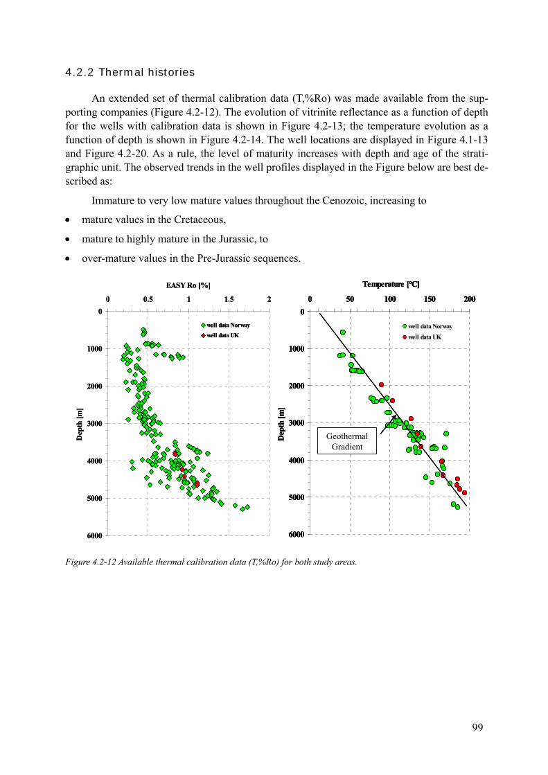
4.2.2 Thermal histories

An extended set of thermal calibration data (T,%Ro) was made available from the sup-porting companies (Figure 4.2-12). The evolution of vitrinite reflectance as a function of depth for the wells with calibration data is shown in Figure 4.2-13; the temperature evolution as a function of depth is shown in Figure 4.2-14. The well locations are displayed in Figure 4.1-13 and Figure 4.2-20. As a rule, the level of maturity increases with depth and age of the strati-graphic unit. The observed trends in the well profiles displayed in the Figure below are best de-scribed as:

Immature to very low mature values throughout the Cenozoic, increasing to

• mature values in the Cretaceous,

• mature to highly mature in the Jurassic, to

• over-mature values in the Pre-Jurassic sequences.

0

1000

2000

3000

4000

5000

6000

0 0.5 1 1.5 2

EASY Ro [%]

Dep

th [m

]

well data Norwaywell data UK

0

1000

2000

3000

4000

5000

6000

0 50 100 150 200

Temperature [°C]D

epth

[m]

well data Norwaywell data UK

Geothermal Gradient

0

1000

2000

3000

4000

5000

6000

0 0.5 1 1.5 2

EASY Ro [%]

Dep

th [m

]

well data Norwaywell data UK

0

1000

2000

3000

4000

5000

6000

0 50 100 150 200

Temperature [°C]D

epth

[m]

well data Norwaywell data UK

Geothermal Gradient

0

1000

2000

3000

4000

5000

6000

0 50 100 150 200

Temperature [°C]D

epth

[m]

well data Norwaywell data UK

Geothermal Gradient

Geothermal Gradient

Figure 4.2-12 Available thermal calibration data (T,%Ro) for both study areas.

99

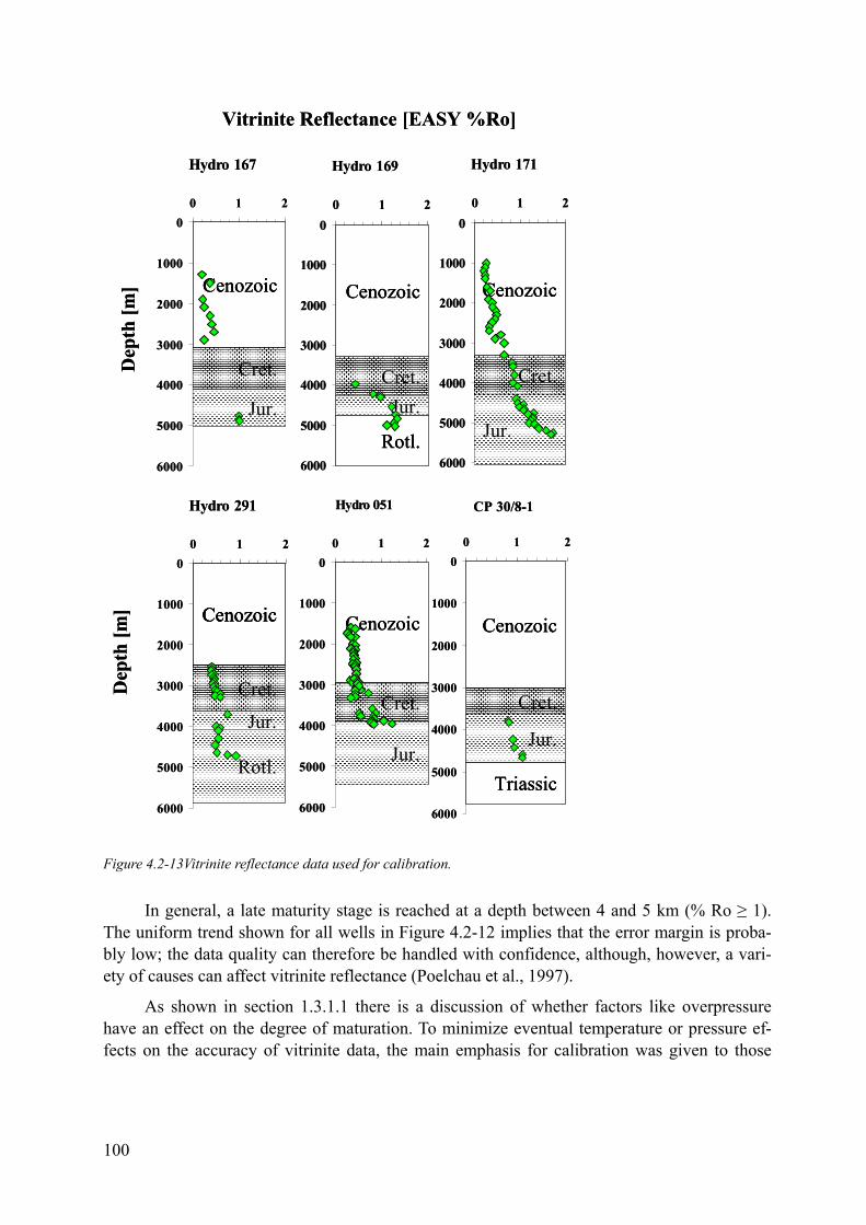
Cret.

Jur.

Cenozoic

Rotl.

Vitrinite Reflectance [EASY %Ro]

Cret.

Jur.

Cenozoic

Cret.Jur.

Cenozoic

Rotl.

Cret.

Jur.

Cenozoic

Dep

th [m

]

Cret.

Jur.

Cenozoic

Cret.

Jur.

Cenozoic

Triassic

Dep

th [m

]

Hydro 167

0

1000

2000

3000

4000

5000

6000

0 1 2

Hydro 169

0

1000

2000

3000

4000

5000

6000

0 1 2

Hydro 171

0

1000

2000

3000

4000

5000

6000

0 1 2

CP 30/8-1

0

1000

2000

3000

4000

5000

6000

0 1 2

Hydro 291

0

1000

2000

3000

4000

5000

6000

0 1 2

Hydro 051

0

1000

2000

3000

4000

5000

6000

0 1 2

Cret.

Jur.

Cenozoic

Rotl.

Cret.

Jur.

Cenozoic

Cret.

Jur.

Cenozoic

Rotl.

Vitrinite Reflectance [EASY %Ro]

Cret.

Jur.

Cenozoic

Cret.

Jur.

Cenozoic

Cret.Jur.

Cenozoic

Rotl.

Cret.Jur.

Cenozoic

Rotl.

Cret.

Jur.

Cenozoic

Cret.

Jur.

Cenozoic

Dep

th [m

]

Cret.

Jur.

Cenozoic

Cret.

Jur.

Cenozoic

Cret.

Jur.

Cenozoic

Triassic

Cret.

Jur.

Cenozoic

Triassic

Dep

th [m

]

Hydro 167

0

1000

2000

3000

4000

5000

6000

0 1 2

Hydro 169

0

1000

2000

3000

4000

5000

6000

0 1 2

Hydro 171

0

1000

2000

3000

4000

5000

6000

0 1 2

CP 30/8-1

0

1000

2000

3000

4000

5000

6000

0 1 2

Hydro 291

0

1000

2000

3000

4000

5000

6000

0 1 2

Hydro 051

0

1000

2000

3000

4000

5000

6000

0 1 2

Figure 4.2-13Vitrinite reflectance data used for calibration.

In general, a late maturity stage is reached at a depth between 4 and 5 km (% Ro ≥ 1). The uniform trend shown for all wells in Figure 4.2-12 implies that the error margin is proba-bly low; the data quality can therefore be handled with confidence, although, however, a vari-ety of causes can affect vitrinite reflectance (Poelchau et al., 1997).

As shown in section 1.3.1.1 there is a discussion of whether factors like overpressure have an effect on the degree of maturation. To minimize eventual temperature or pressure ef-fects on the accuracy of vitrinite data, the main emphasis for calibration was given to those

100

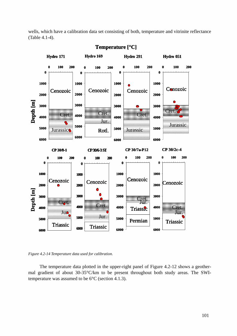
101

wells, which have a calibration data set consisting of both, temperature and vitrinite reflectance (Table 4.1-4).

Dep

th [m

]

Hydro 169

0

1000

2000

3000

4000

5000

6000

0 100 200

Cret.Jur.

Cenozoic

Triassic

Cret.

Jur.

Cenozoic

Triassic

Cret.Jur.

Cenozoic

Triassic

Permian

Cret.

Jurassic

Cenozoic

Cret.

Jurassic

Cenozoic

Cret.

Jurassic

Cenozoic

Cret.Jur.

Cenozoic

Rotl.

Temperature [°C]

Dep

th [m

]

Hydro 171

0

1000

2000

3000

4000

5000

6000

0 100 200

Hydro 291

0

1000

2000

3000

4000

5000

6000

0 100 200

Hydro 051

0

1000

2000

3000

4000

5000

6000

0 100 200

CP 30/6-3 ST

0

1000

2000

3000

4000

5000

6000

0 100 200

CP 30/7a-P12

0

1000

2000

3000

4000

5000

6000

0 100 200

Cret.

Jur.

Cenozoic

Triassic

0

1000

2000

3000

4000

5000

6000

0 100 200

CP 30/8-1 CP 30/2c-4

0

1000

2000

3000

4000

5000

6000

0 100 200

Dep

th [m

]

Hydro 169

0

1000

2000

3000

4000

5000

6000

0 100 200

Cret.Jur.

Cenozoic

Triassic

Cret.

Jur.

Cenozoic

Triassic

Cret.Jur.

Cenozoic

Triassic

Permian

Cret.

Jurassic

Cenozoic

Cret.

Jurassic

Cenozoic

Cret.

Jurassic

Cenozoic

Cret.Jur.

Cenozoic

Rotl.

Temperature [°C]

Dep

th [m

]

Hydro 171

0

1000

2000

3000

4000

5000

6000

0 100 200

Hydro 291

0

1000

2000

3000

4000

5000

6000

0 100 200

Hydro 051

0

1000

2000

3000

4000

5000

6000

0 100 200

CP 30/6-3 ST

0

1000

2000

3000

4000

5000

6000

0 100 200

CP 30/7a-P12

0

1000

2000

3000

4000

5000

6000

0 100 200

Cret.

Jur.

Cenozoic

Triassic

0

1000

2000

3000

4000

5000

6000

0 100 200

CP 30/8-1 CP 30/2c-4

0

1000

2000

3000

4000

5000

6000

0 100 200

Hydro 169

0

1000

2000

3000

4000

5000

6000

0 100 200

Cret.Jur.

Cenozoic

Triassic

Cret.Jur.

Cenozoic

Triassic

Cret.

Jur.

Cenozoic

Triassic

Cret.

Jur.

Cenozoic

Triassic

Cret.Jur.

Cenozoic

Triassic

Permian

Cret.Jur.

Cenozoic

Triassic

Cret.Jur.

Cenozoic

Triassic

Permian

Cret.

Jurassic

Cenozoic

Cret.

Jurassic

Cenozoic

Cret.

Jurassic

Cenozoic

Cret.

Jurassic

Cenozoic

Cret.

Jurassic

Cenozoic

Cret.

Jurassic

Cenozoic

Cret.Jur.

Cenozoic

Rotl.

Cret.Jur.

Cenozoic

Rotl.

Temperature [°C]

Dep

th [m

]

Hydro 171

0

1000

2000

3000

4000

5000

6000

0 100 200

Hydro 291

0

1000

2000

3000

4000

5000

6000

0 100 200

Hydro 051

0

1000

2000

3000

4000

5000

6000

0 100 200

CP 30/6-3 ST

0

1000

2000

3000

4000

5000

6000

0 100 200

CP 30/7a-P12

0

1000

2000

3000

4000

5000

6000

0 100 200

Cret.

Jur.

Cenozoic

Triassic

0

1000

2000

3000

4000

5000

6000

0 100 200

CP 30/8-1

Cret.

Jur.

Cenozoic

Triassic

Cret.

Jur.

Cenozoic

Triassic

0

1000

2000

3000

4000

5000

6000

0 100 200

CP 30/8-1 CP 30/2c-4

0

1000

2000

3000

4000

5000

6000

0 100 200

Figure 4.2-14 Temperature data used for calibration.

The temperature data plotted in the upper-right panel of Figure 4.2-12 shows a geother-mal gradient of about 30-35°C/km to be present throughout both study areas. The SWI-temperature was assumed to be 6°C (section 4.1.3).

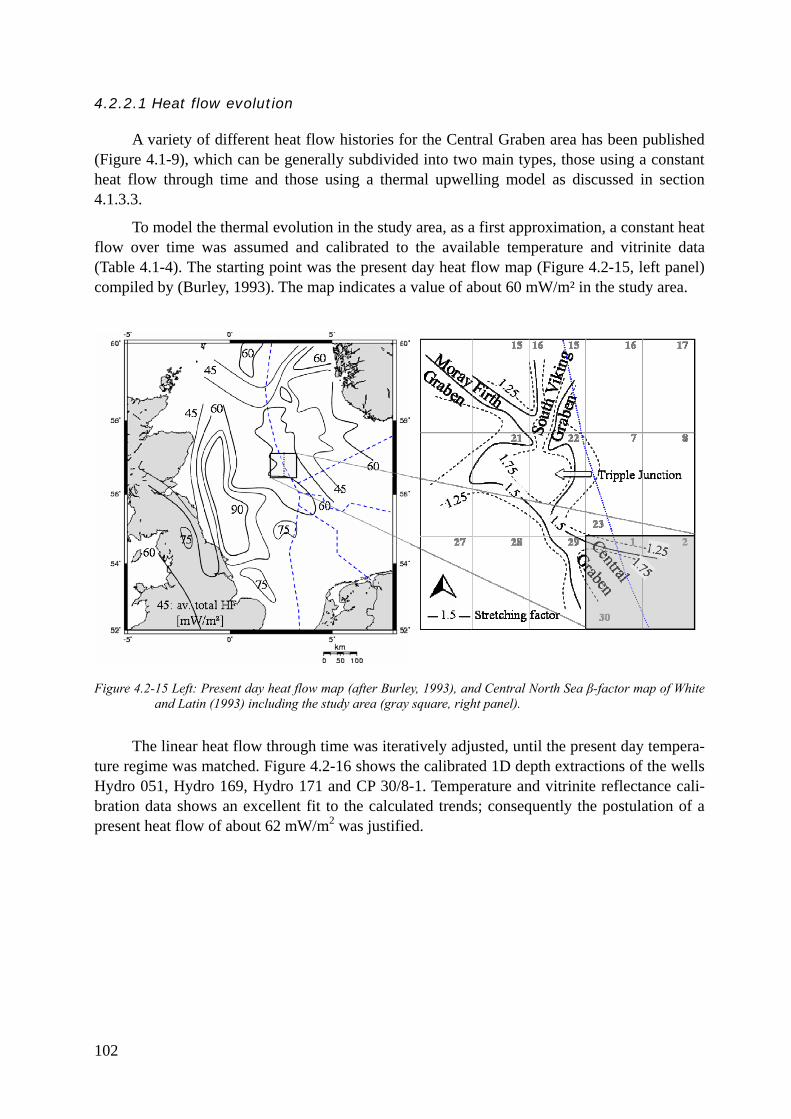
102

4.2.2.1 Heat flow evolution

A variety of different heat flow histories for the Central Graben area has been published (Figure 4.1-9), which can be generally subdivided into two main types, those using a constant heat flow through time and those using a thermal upwelling model as discussed in section 4.1.3.3.

To model the thermal evolution in the study area, as a first approximation, a constant heat flow over time was assumed and calibrated to the available temperature and vitrinite data (Table 4.1-4). The starting point was the present day heat flow map (Figure 4.2-15, left panel) compiled by (Burley, 1993). The map indicates a value of about 60 mW/m² in the study area.

Figure 4.2-15 Left: Present day heat flow map (after Burley, 1993), and Central North Sea β-factor map of White and Latin (1993) including the study area (gray square, right panel).

The linear heat flow through time was iteratively adjusted, until the present day tempera-ture regime was matched. Figure 4.2-16 shows the calibrated 1D depth extractions of the wells Hydro 051, Hydro 169, Hydro 171 and CP 30/8-1. Temperature and vitrinite reflectance cali-bration data shows an excellent fit to the calculated trends; consequently the postulation of a present heat flow of about 62 mW/m2 was justified.

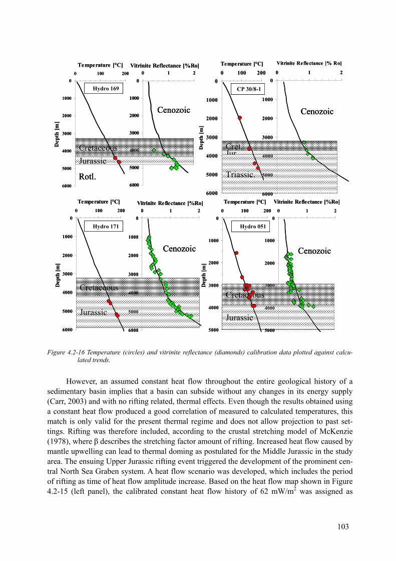
Cretaceous

Jurassic

Cenozoic

Cretaceous

Jurassic

Cenozoic

0

1000

2000

3000

4000

5000

6000

0 100 200

Temperature [°C]

Dep

th [m

]

0

1000

2000

3000

4000

5000

6000

0 1 2Vitrinite Reflectance [%Ro]

CretaceousJurassic

Cenozoic

Rotl.

0

1000

2000

3000

4000

5000

6000

0 1 2Vitrinite Reflectance [%Ro]

0

1000

2000

3000

4000

5000

6000

0 100 200

Temperature [°C]D

epth

[m]

Hydro 169

Hydro 1710

1000

2000

3000

4000

5000

0 100 200

Temperature [°C]D

epth

[m]

0

1000

2000

3000

4000

5000

0 1 2

Vitrinite Reflectance [%Ro]

Hydro 051

Cret.Jur.

Cenozoic

Triassic.

0

1000

2000

3000

4000

5000

6000

0 1

Vitrinite Reflectance [% Ro]

2

0

1000

2000

3000

4000

5000

6000

0 100 200

Temperature [°C]

Dep

th [m

]

CP 30/8-1

Cretaceous

Jurassic

Cenozoic

Cretaceous

Jurassic

Cenozoic

Cretaceous

Jurassic

Cenozoic

Cretaceous

Jurassic

Cenozoic

0

1000

2000

3000

4000

5000

6000

0 100 200

Temperature [°C]

Dep

th [m

]

0

1000

2000

3000

4000

5000

6000

0 1 2Vitrinite Reflectance [%Ro]

CretaceousJurassic

Cenozoic

Rotl.

CretaceousJurassic

Cenozoic

Rotl.

0

1000

2000

3000

4000

5000

6000

0 1 2Vitrinite Reflectance [%Ro]

0

1000

2000

3000

4000

5000

6000

0 100 200

Temperature [°C]D

epth

[m]

Hydro 169

Hydro 1710

1000

2000

3000

4000

5000

0 100 200

Temperature [°C]D

epth

[m]

0

1000

2000

3000

4000

5000

0 1 2

Vitrinite Reflectance [%Ro]

Hydro 051

Cret.Jur.

Cenozoic

Triassic.

Cret.Jur.

Cenozoic

Triassic.

0

1000

2000

3000

4000

5000

6000

0 1

Vitrinite Reflectance [% Ro]

2

0

1000

2000

3000

4000

5000

6000

0 100 200

Temperature [°C]

Dep

th [m

]

CP 30/8-1

Figure 4.2-16 Temperature (circles) and vitrinite reflectance (diamonds) calibration data plotted against calcu-lated trends.

However, an assumed constant heat flow throughout the entire geological history of a sedimentary basin implies that a basin can subside without any changes in its energy supply (Carr, 2003) and with no rifting related, thermal effects. Even though the results obtained using a constant heat flow produced a good correlation of measured to calculated temperatures, this match is only valid for the present thermal regime and does not allow projection to past set-tings. Rifting was therefore included, according to the crustal stretching model of McKenzie (1978), where β describes the stretching factor amount of rifting. Increased heat flow caused by mantle upwelling can lead to thermal doming as postulated for the Middle Jurassic in the study area. The ensuing Upper Jurassic rifting event triggered the development of the prominent cen-tral North Sea Graben system. A heat flow scenario was developed, which includes the period of rifting as time of heat flow amplitude increase. Based on the heat flow map shown in Figure 4.2-15 (left panel), the calibrated constant heat flow history of 62 mW/m2 was assigned as

103

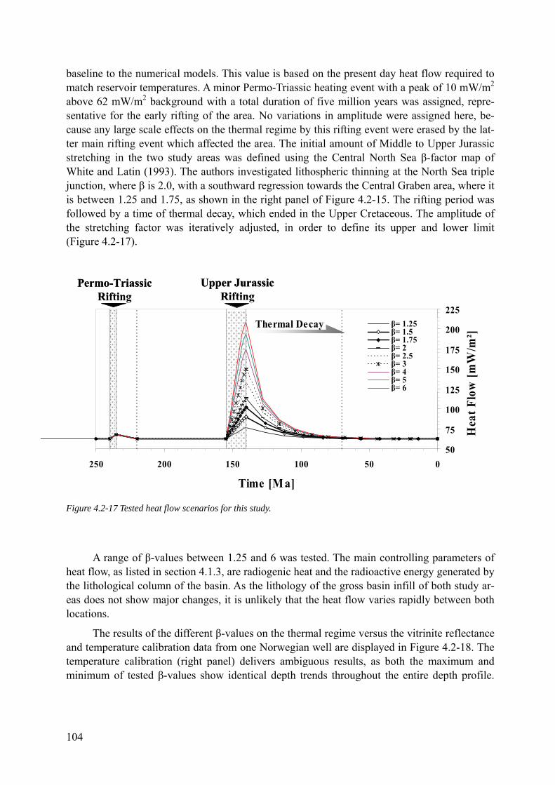
104

baseline to the numerical models. This value is based on the present day heat flow required to match reservoir temperatures. A minor Permo-Triassic heating event with a peak of 10 mW/m2 above 62 mW/m2 background with a total duration of five million years was assigned, repre-sentative for the early rifting of the area. No variations in amplitude were assigned here, be-cause any large scale effects on the thermal regime by this rifting event were erased by the lat-ter main rifting event which affected the area. The initial amount of Middle to Upper Jurassic stretching in the two study areas was defined using the Central North Sea β-factor map of White and Latin (1993). The authors investigated lithospheric thinning at the North Sea triple junction, where β is 2.0, with a southward regression towards the Central Graben area, where it is between 1.25 and 1.75, as shown in the right panel of Figure 4.2-15. The rifting period was followed by a time of thermal decay, which ended in the Upper Cretaceous. The amplitude of the stretching factor was iteratively adjusted, in order to define its upper and lower limit (Figure 4.2-17).

50

75

100

125

150

175

200

225

050100150200250

Time [Ma]H

eat F

low

[mW

/m²]

β= 1.25β= 1.5β= 1.75β= 2β= 2.5β= 3β= 4β= 5β= 6

Thermal Decay

Permo-Triassic Rifting

Upper Jurassic Rifting

50

75

100

125

150

175

200

225

050100150200250

Time [Ma]H

eat F

low

[mW

/m²]

β= 1.25β= 1.5β= 1.75β= 2β= 2.5β= 3β= 4β= 5β= 6

Thermal Decay

Permo-Triassic Rifting

Upper Jurassic Rifting

Figure 4.2-17 Tested heat flow scenarios for this study.

A range of β-values between 1.25 and 6 was tested. The main controlling parameters of heat flow, as listed in section 4.1.3, are radiogenic heat and the radioactive energy generated by the lithological column of the basin. As the lithology of the gross basin infill of both study ar-eas does not show major changes, it is unlikely that the heat flow varies rapidly between both locations.

The results of the different β-values on the thermal regime versus the vitrinite reflectance and temperature calibration data from one Norwegian well are displayed in Figure 4.2-18. The temperature calibration (right panel) delivers ambiguous results, as both the maximum and minimum of tested β-values show identical depth trends throughout the entire depth profile.

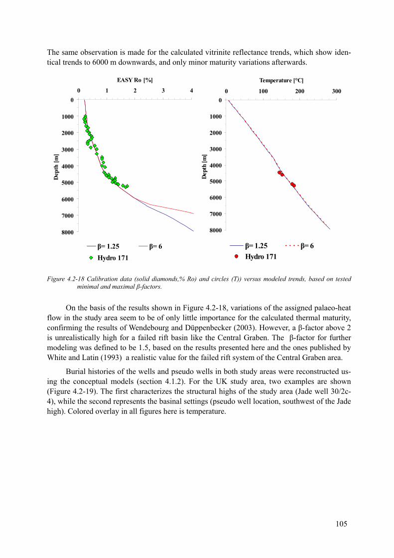
105

The same observation is made for the calculated vitrinite reflectance trends, which show iden-tical trends to 6000 m downwards, and only minor maturity variations afterwards.

0

1000

2000

3000

4000

5000

6000

7000

8000

0 1 2 3 4

EASY Ro [%]

Dep

th [m

]

β= 1.25 β= 6Hydro 171

0

1000

2000

3000

4000

5000

6000

7000

8000

0 100 200 300

Temperature [°C]

Dept

h [m

]

β= 1.25 β= 6Hydro 171

0

1000

2000

3000

4000

5000

6000

7000

8000

0 1 2 3 4

EASY Ro [%]

Dep

th [m

]

β= 1.25 β= 6Hydro 171

0

1000

2000

3000

4000

5000

6000

7000

8000

0 100 200 300

Temperature [°C]

Dept

h [m

]

β= 1.25 β= 6Hydro 171

Figure 4.2-18 Calibration data (solid diamonds,% Ro) and circles (T)) versus modeled trends, based on tested minimal and maximal β-factors.

On the basis of the results shown in Figure 4.2-18, variations of the assigned palaeo-heat flow in the study area seem to be of only little importance for the calculated thermal maturity, confirming the results of Wendebourg and Düppenbecker (2003). However, a β-factor above 2 is unrealistically high for a failed rift basin like the Central Graben. The β-factor for further modeling was defined to be 1.5, based on the results presented here and the ones published by White and Latin (1993) a realistic value for the failed rift system of the Central Graben area.

Burial histories of the wells and pseudo wells in both study areas were reconstructed us-ing the conceptual models (section 4.1.2). For the UK study area, two examples are shown (Figure 4.2-19). The first characterizes the structural highs of the study area (Jade well 30/2c-4), while the second represents the basinal settings (pseudo well location, southwest of the Jade high). Colored overlay in all figures here is temperature.

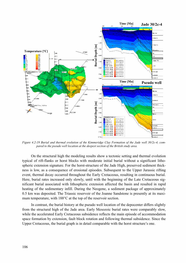
Jade 30/2c-4

Pseudo well

Temperature [°C]

Bur

ial D

epth

[m]

Bur

ial D

epth

[m]

Time [Ma]

Time [Ma] Jade 30/2c-4

Pseudo well

Temperature [°C]

Bur

ial D

epth

[m]

Bur

ial D

epth

[m]

Time [Ma]

Time [Ma]

Figure 4.2-19 Burial and thermal evolution of the Kimmeridge Clay Formation of the Jade well 30/2c-4, com-

pared to the pseudo well location at the deepest section of the British study area.

On the structural high the modeling results show a tectonic setting and thermal evolution typical of rift-flanks or horst blocks with moderate initial burial without a significant litho-spheric extension signature. For the horst-structure of the Jade High, preserved sediment thick-ness is low, as a consequence of erosional episodes. Subsequent to the Upper Jurassic rifting event, thermal decay occurred throughout the Early Cretaceous, resulting in continuous burial. Here, burial rates increased only slowly, until with the beginning of the Late Cretaceous sig-nificant burial associated with lithospheric extension affected the basin and resulted in rapid heating of the sedimentary infill. During the Neogene, a sediment package of approximately 0.5 km was deposited. The Triassic reservoir of the Joanne Sandstone is presently at its maxi-mum temperature, with 188°C at the top of the reservoir section.

In contrast, the burial history at the pseudo well location of the depocenter differs slightly from the structural high of the Jade area. Early Mesozoic burial rates were comparably slow, while the accelerated Early Cretaceous subsidence reflects the main episode of accommodation space formation by extension, fault block rotation and following thermal subsidence. Since the Upper Cretaceous, the burial graph is in detail comparable with the horst structure’s one.

106

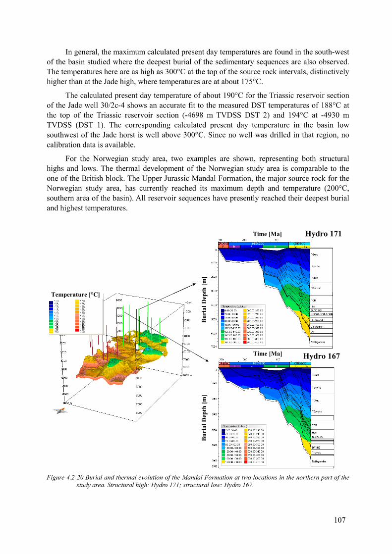
In general, the maximum calculated present day temperatures are found in the south-west of the basin studied where the deepest burial of the sedimentary sequences are also observed. The temperatures here are as high as 300°C at the top of the source rock intervals, distinctively higher than at the Jade high, where temperatures are at about 175°C.

The calculated present day temperature of about 190°C for the Triassic reservoir section of the Jade well 30/2c-4 shows an accurate fit to the measured DST temperatures of 188°C at the top of the Triassic reservoir section (-4698 m TVDSS DST 2) and 194°C at -4930 m TVDSS (DST 1). The corresponding calculated present day temperature in the basin low southwest of the Jade horst is well above 300°C. Since no well was drilled in that region, no calibration data is available.

For the Norwegian study area, two examples are shown, representing both structural highs and lows. The thermal development of the Norwegian study area is comparable to the one of the British block. The Upper Jurassic Mandal Formation, the major source rock for the Norwegian study area, has currently reached its maximum depth and temperature (200°C, southern area of the basin). All reservoir sequences have presently reached their deepest burial and highest temperatures.

Hydro 171

Hydro 167

Temperature [°C]

Bur

ial D

epth

[m]

Bur

ial D

epth

[m]

Time [Ma]

Time [Ma] Hydro 171

Hydro 167

Temperature [°C]

Bur

ial D

epth

[m]

Bur

ial D

epth

[m]

Time [Ma]

Time [Ma]

Figure 4.2-20 Burial and thermal evolution of the Mandal Formation at two locations in the northern part of the

study area. Structural high: Hydro 171; structural low: Hydro 167.

107

The close correlation of the calculated and observed temperatures for both areas suggests that the assignment of the same heat flow history to both study areas was justified.

4.2.3 Maturation & filling histories

4.2.3.1 Published compositional kinetic models

In the first simulation runs, published compositional kinetic models were assigned to the different source rock intervals in the basin models to evaluate hydrocarbon generation, migra-tion and phase behavior as a function of time. In order to assess the migration histories of both areas, first the drainage areas and subsequently the migration paths of the generated hydrocar-bons were modeled.

The carrier map of the Triassic Joanne Sandstone of the UK model was divided into drainage areas, using the PetroCharge tool of the PetroMod™ modeling software package. This tool models migration as flow within a defined carrier. The calculated drainage area borders, the closures, showing areas of possible hydrocarbon accumulations and the calculated spill paths, are based on the present day topography. Migration is assumed to occur instantaneously. Such flowpath models are based on the assumption, that

• petroleum flows against a defined surface (e.g. a regional seal),

• and that migration is only buoyancy driven (flow is generally up-dip) (IES, 2002).

The model’s basin sides were left open in all simulation runs, generated petroleum mi-grating to the model’s margins could therefore leave the basin through the open sides, thereby preventing artificially trapped accumulations in the model boundaries.

Subsequent to the calibration of the model, especially of those parameters crucial for the timing of hydrocarbon generation, the temperature boundary conditions, compositional kinetic models for the specific source-rock kerogen, as defined in section 4.1.7, were assigned to the source rock facies in the basin models in order to model the source rock’s maturation and tim-ing of generation and expulsion of hydrocarbons. For the first runs, faults were assigned to the model; their properties were defined in individual sensitivity runs as open (permeable) and closed (impermeable) with respect to petroleum migration. In comparison to the model without faults, no significant effects on the migration pattern or composition of the accumulated hydro-carbons could be proven. The assignment of faults only resulted in insignificantly smaller hy-drocarbon accumulations, but significantly longer calculation times. Therefore, no faults were assigned to the basin models for the further runs.

108

Figure 4.2-21 Left: Present day drainage areas of the Joanne Sandstone (UK study area). Right: 3D view on UK drainage areas, including closures, hydrocarbon accumulations and migration pathways. The map shows the topography of the Triassic Joanne sandstone (temperature overlay). The transparent layer on the top is the Heather Formation. The polygons are the individual drainage areas. The bigger, dot-ted polygon shows the kitchen area for the Jade structure, white arrows show the migration paths, the dotted arrow shows the fill path to the Judy structure in the British model.

Figure 4.2-21 shows the result from the drainage area modeling. The left panel in Figure 4.2-21 shows the Triassic Sandstone layer of the British 3D model at present day depth, includ-ing the drainage areas, displayed here as black polygons, the light grey areas represent oil ac-cumulations, the dark grey areas gas accumulations. The predicted accumulations are con-firmed by the wells of the Jade and Judy structures. The black arrows show migration paths of the hydrocarbons. Fill spill occurs at spill points, connecting several accumulations in up-dip direction. The right panel of Figure 4.2-21 shows the same area in a 3D perspective. The area enclosed by the white dotted line is the deep kitchen area for the Jade prospect. The burial graphs and corresponding temperature trends through time for the centre and flanks of this area were shown in Figure 4.2-19. Results of 3D modeling indicate that the kitchen area of the Jade field is the deep basin southeast of the structure. The Judy field is sourced from three directions (Figure 4.2-21). Previous investigations showed that the fluids present in the pre-Cretaceous reservoirs of both structures are geochemically similar (ConocoPhillips pers. com.), a fact which is supported by the spill route from Jade to Judy/Joanne.

109

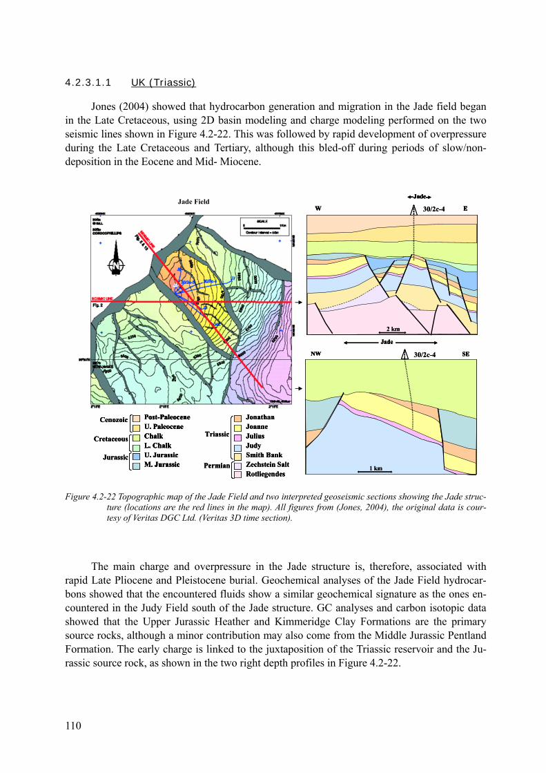
4.2.3.1.1 UK (Triassic)

Jones (2004) showed that hydrocarbon generation and migration in the Jade field began in the Late Cretaceous, using 2D basin modeling and charge modeling performed on the two seismic lines shown in Figure 4.2-22. This was followed by rapid development of overpressure during the Late Cretaceous and Tertiary, although this bled-off during periods of slow/non-deposition in the Eocene and Mid- Miocene.

2 km

Jade

W E

2 km2 km2 km

Jade

W E

1 km

NW SE

Jade

1 km1 km1 km

NW SE

Jade

Post-PaleoceneU. PaleoceneChalkL. ChalkU. JurassicM. Jurassic

Cretaceous

Jurassic

Cenozoic JonathanJoanneJuliusJudySmith BankZechstein SaltRotliegendes

Permian

Triassic

30/2c-4

30/2c-4Jade Field

2 km

Jade

W E

2 km2 km2 km

Jade

W E

1 km

NW SE

Jade

1 km1 km1 km

NW SE

Jade

Post-PaleoceneU. PaleoceneChalkL. ChalkU. JurassicM. Jurassic

Cretaceous

Jurassic

Cenozoic Post-PaleoceneU. PaleoceneChalkL. ChalkU. JurassicM. Jurassic

Post-PaleoceneU. PaleoceneChalkL. ChalkU. JurassicM. Jurassic

Cretaceous

Jurassic

Cenozoic JonathanJoanneJuliusJudySmith BankZechstein SaltRotliegendes

Permian

Triassic

JonathanJoanneJuliusJudySmith BankZechstein SaltRotliegendes

Permian

Triassic

30/2c-4

30/2c-4Jade Field

Figure 4.2-22 Topographic map of the Jade Field and two interpreted geoseismic sections showing the Jade struc-ture (locations are the red lines in the map). All figures from (Jones, 2004), the original data is cour-tesy of Veritas DGC Ltd. (Veritas 3D time section).

The main charge and overpressure in the Jade structure is, therefore, associated with rapid Late Pliocene and Pleistocene burial. Geochemical analyses of the Jade Field hydrocar-bons showed that the encountered fluids show a similar geochemical signature as the ones en-countered in the Judy Field south of the Jade structure. GC analyses and carbon isotopic data showed that the Upper Jurassic Heather and Kimmeridge Clay Formations are the primary source rocks, although a minor contribution may also come from the Middle Jurassic Pentland Formation. The early charge is linked to the juxtaposition of the Triassic reservoir and the Ju-rassic source rock, as shown in the two right depth profiles in Figure 4.2-22.

110

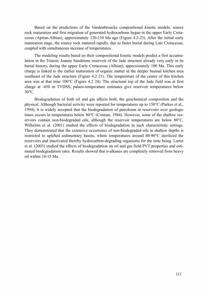
Based on the predictions of the Vandenbroucke compositional kinetic models, source rock maturation and first migration of generated hydrocarbons began in the upper Early Creta-ceous (Aptian-Albian), approximately 120-110 Ma ago (Figure 4.2-23). After the initial early maturation stage, the source rock matured rapidly, due to faster burial during Late Cretaceous, coupled with simultaneous increase of temperatures.

The modeling results based on their compositional kinetic models predict a first accumu-lation in the Triassic Joanne Sandstone reservoir of the Jade structure already very early in its burial history, during the upper Early Cretaceous (Albian), approximately 100 Ma. This early charge is linked to the earlier maturation of organic matter in the deeper basinal kitchen area southeast of the Jade structure (Figure 4.2 21). The temperature of the center of this kitchen area was at that time 100°C (Figure 4.2 24). The structural top of the Jade field was at first charge at -450 m TVDSS, palaeo-temperature estimates give reservoir temperatures below 30°C.

Biodegradation of both oil and gas affects both, the geochemical composition and the physical. Although bacterial activity were reported for temperatures up to 150°C (Parkes et al., 1994), it is widely accepted that the biodegradation of petroleum in reservoirs over geologic times occurs in temperatures below 80°C (Connan, 1984). However, some of the shallow res-ervoirs contain non-biodegraded oils, although the reservoir temperatures are below 80°C. Wilhelms et al. (2001) studied the effects of biodegradation in such characteristic settings. They demonstrated that the extensive occurrence of non-biodegraded oils in shallow depths is restricted to uplifted sedimentary basins, where temperatures around 80-90°C sterilized the reservoirs and inactivated thereby hydrocarbon-degrading organisms for the time being. Larter et al. (2003) studied the effects of biodegradation on oil and gas field PVT properties and esti-mated biodegradation rates. Results showed that n-alkanes are completely removed from heavy oil within 10-15 Ma.

111

Figure 4.2-23 EASY Ro and temperature of the Heather Formation, approximately 110 Ma ago. Vitrinite reflec-

tance shows an early maturation stage in the basin southwest of Jade and West of Judy.

112

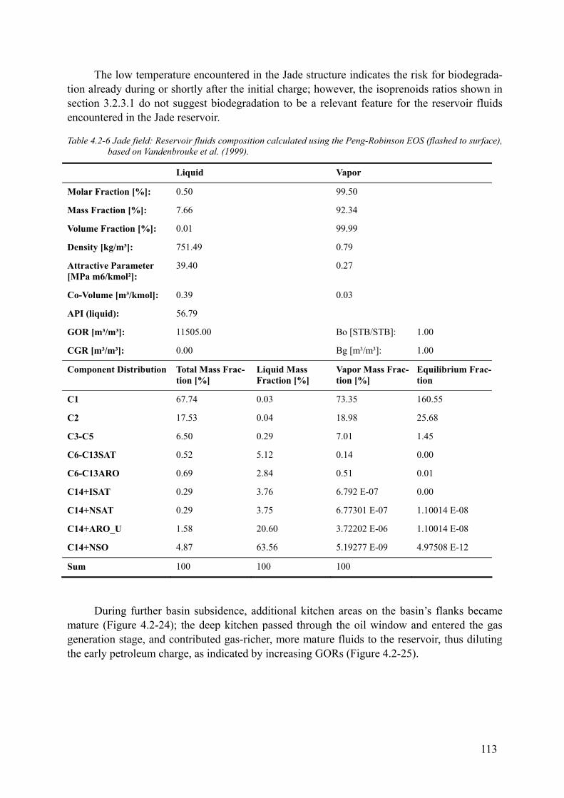
The low temperature encountered in the Jade structure indicates the risk for biodegrada-tion already during or shortly after the initial charge; however, the isoprenoids ratios shown in section 3.2.3.1 do not suggest biodegradation to be a relevant feature for the reservoir fluids encountered in the Jade reservoir.

Table 4.2-6 Jade field: Reservoir fluids composition calculated using the Peng-Robinson EOS (flashed to surface), based on Vandenbrouke et al. (1999).

Liquid Vapor

Molar Fraction [%]: 0.50 99.50

Mass Fraction [%]: 7.66 92.34

Volume Fraction [%]: 0.01 99.99

Density [kg/m³]: 751.49 0.79

Attractive Parameter [MPa m6/kmol²]:

39.40 0.27

Co-Volume [m³/kmol]: 0.39 0.03

API (liquid): 56.79

GOR [m³/m³]: 11505.00 Bo [STB/STB]: 1.00

CGR [m³/m³]: 0.00 Bg [m³/m³]: 1.00

Component Distribution Total Mass Frac-tion [%]

Liquid Mass Fraction [%]

Vapor Mass Frac-tion [%]

Equilibrium Frac-tion

C1 67.74 0.03 73.35 160.55

C2 17.53 0.04 18.98 25.68

C3-C5 6.50 0.29 7.01 1.45

C6-C13SAT 0.52 5.12 0.14 0.00

C6-C13ARO 0.69 2.84 0.51 0.01

C14+ISAT 0.29 3.76 6.792 E-07 0.00

C14+NSAT 0.29 3.75 6.77301 E-07 1.10014 E-08

C14+ARO_U 1.58 20.60 3.72202 E-06 1.10014 E-08

C14+NSO 4.87 63.56 5.19277 E-09 4.97508 E-12

Sum 100 100 100

During further basin subsidence, additional kitchen areas on the basin’s flanks became mature (Figure 4.2-24); the deep kitchen passed through the oil window and entered the gas generation stage, and contributed gas-richer, more mature fluids to the reservoir, thus diluting the early petroleum charge, as indicated by increasing GORs (Figure 4.2-25).

113

050100150200250300350

0255075100125150175

Time [Ma]

Tem

pera

ture

[°C

]

0

2000

4000

6000

8000

10000

Dep

th [m

]

Center Heather Temperature Flank Heather TemperatureCenter Heather Depth Flank Heather Depth

Figure 4.2-24 Temperature and burial development of the Heather Formation at the center and at the flanks of the

kitchen area of the Jade structure.

950750

0.1

1

10

100

1000

10000

100000

020406080100

Time [Ma]

GO

R [S

m³/S

m³]

Jade GOR Jade GOR [field]Judy GOR Judy GOR [field]

Figure 4.2-25 GOR evolution of the British Triassic reservoir fluids, as predicted by the assigned Vandenbroucke

compositional kinetic models.

The cracking of oil as a result of rising temperatures led to the onset of overpressure by enhance gas generation during the Late Cretaceous, resulting in the sudden switch from light oil to dry gas, leaving finally dry gas to be the only hydrocarbon phase in the reservoir with a GOR of 11,505 Sm³/Sm³ and 56° API Gravity for present times, as predicted by the composi-tional kinetic models of Vandenbroucke et al. (1999), as presented in Table 4.2-6 and Figure 4.2-25.

114

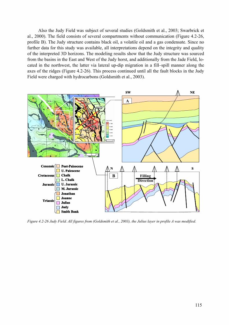
Also the Judy Field was subject of several studies (Goldsmith et al., 2003; Swarbrick et al., 2000). The field consists of several compartments without communication (Figure 4.2-26, profile B). The Judy structure contains black oil, a volatile oil and a gas condensate. Since no further data for this study was available, all interpretations depend on the integrity and quality of the interpreted 3D horizons. The modeling results show that the Judy structure was sourced from the basins in the East and West of the Judy horst, and additionally from the Jade Field, lo-cated in the northwest, the latter via lateral up-dip migration in a fill–spill manner along the axes of the ridges (Figure 4.2-26). This process continued until all the fault blocks in the Judy Field were charged with hydrocarbons (Goldsmith et al., 2003).

Post-PaleoceneU. PaleoceneChalkL. ChalkU. JurassicM. Jurassic

Cretaceous

Jurassic

Cenozoic

Triassic

JonathanJoanneJuliusJudySmith Bank

SW NE

N S

B Filling Direction

A

Post-PaleoceneU. PaleoceneChalkL. ChalkU. JurassicM. Jurassic

Cretaceous

Jurassic

Cenozoic

Triassic

JonathanJoanneJuliusJudySmith Bank

Post-PaleoceneU. PaleoceneChalkL. ChalkU. JurassicM. Jurassic

Cretaceous

Jurassic

Cenozoic

Triassic

JonathanJoanneJuliusJudySmith Bank

SW NE

N S

B Filling Direction

A

Figure 4.2-26 Judy Field. All figures from (Goldsmith et al., 2003), the Julius layer in profile A was modified.

115

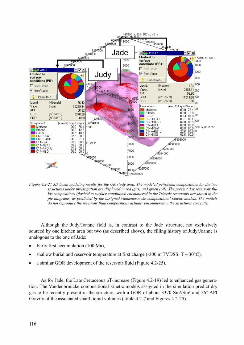
Judy

Jade

Judy

Jade

Figure 4.2-27 3D basin modeling results for the UK study area. The modeled petroleum compositions for the two structures under investigation are displayed in red (gas) and green (oil). The present day reservoir flu-ids compositions (flashed to surface conditions) encountered in the Triassic reservoirs are shown in the pie diagrams, as predicted by the assigned Vandenbroucke compositional kinetic models. The models do not reproduce the reservoir fluid compositions actually encountered in the structures correctly.

Although the Judy/Joanne field is, in contrast to the Jade structure, not exclusively sourced by one kitchen area but two (as described above), the filling history of Judy/Joanne is analogous to the one of Jade:

• Early first accumulation (100 Ma),

• shallow burial and reservoir temperature at first charge (-300 m TVDSS; T ~ 30°C),

• a similar GOR development of the reservoir fluid (Figure 4.2-25).

As for Jade, the Late Cretaceous pT-increase (Figure 4.2-19) led to enhanced gas genera-tion. The Vandenbroucke compositional kinetic models assigned in the simulation predict dry gas to be recently present in the structure, with a GOR of about 3370 Sm³/Sm³ and 56° API Gravity of the associated small liquid volumes (Table 4.2-7 and Figures 4.2-25).

116

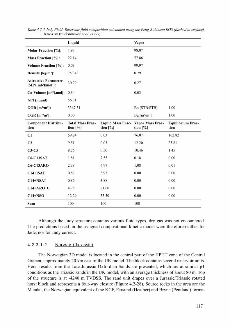
Table 4.2-7 Judy Field: Reservoir fluid composition calculated using the Peng-Robinson EOS (flashed to surface), based on Vandenbrouke et al. (1999).

Liquid Vapor

Molar Fraction [%]: 1.93 98.07

Mass Fraction [%]: 22.14 77.86

Volume Fraction [%]: 0.03 99.97

Density [kg/m³]: 753.43 0.79

Attractive Parameter [MPa m6/kmol²]: 30.79 0.27

Co-Volume [m³/kmol]: 0.34 0.03

API (liquid): 56.31

GOR [m³/m³]: 3367.51 Bo [STB/STB]: 1.00

CGR [m³/m³]: 0.00 Bg [m³/m³]: 1.00

Component Distribu-tion

Total Mass Frac-tion [%]

Liquid Mass Frac-tion [%]

Vapor Mass Frac-tion [%]

Equilibrium Frac-tion

C1 59.24 0.03 76.07 162.82

C2 9.51 0.03 12.20 25.81

C3-C5 8.26 0.50 10.46 1.45

C6-C13SAT 1.81 7.55 0.18 0.00

C6-C13ARO 2.38 6.97 1.08 0.01

C14+ISAT 0.87 3.93 0.00 0.00

C14+NSAT 0.86 3.88 0.00 0.00

C14+ARO_U 4.78 21.60 0.00 0.00

C14+NSO 12.29 55.50 0.00 0.00

Sum 100 100 100

Although the Judy structure contains various fluid types, dry gas was not encountered. The predictions based on the assigned compositional kinetic model were therefore neither for Jade, nor for Judy correct.

4.2.3.1.2 Norway (Jurassic)

The Norwegian 3D model is located in the central part of the HPHT zone of the Central Graben, approximately 20 km east of the UK model. The block contains several reservoir units. Here, results from the Late Jurassic Oxfordian Sands are presented, which are at similar pT conditions as the Triassic sands in the UK model, with an average thickness of about 80 m. Top of the structure is at -4240 m TVDSS. The sand unit drapes over a Jurassic/Triassic rotated horst block and represents a four-way closure (Figure 4.2-28). Source rocks in the area are the Mandal, the Norwegian equivalent of the KCF, Farsund (Heather) and Bryne (Pentland) forma-

117

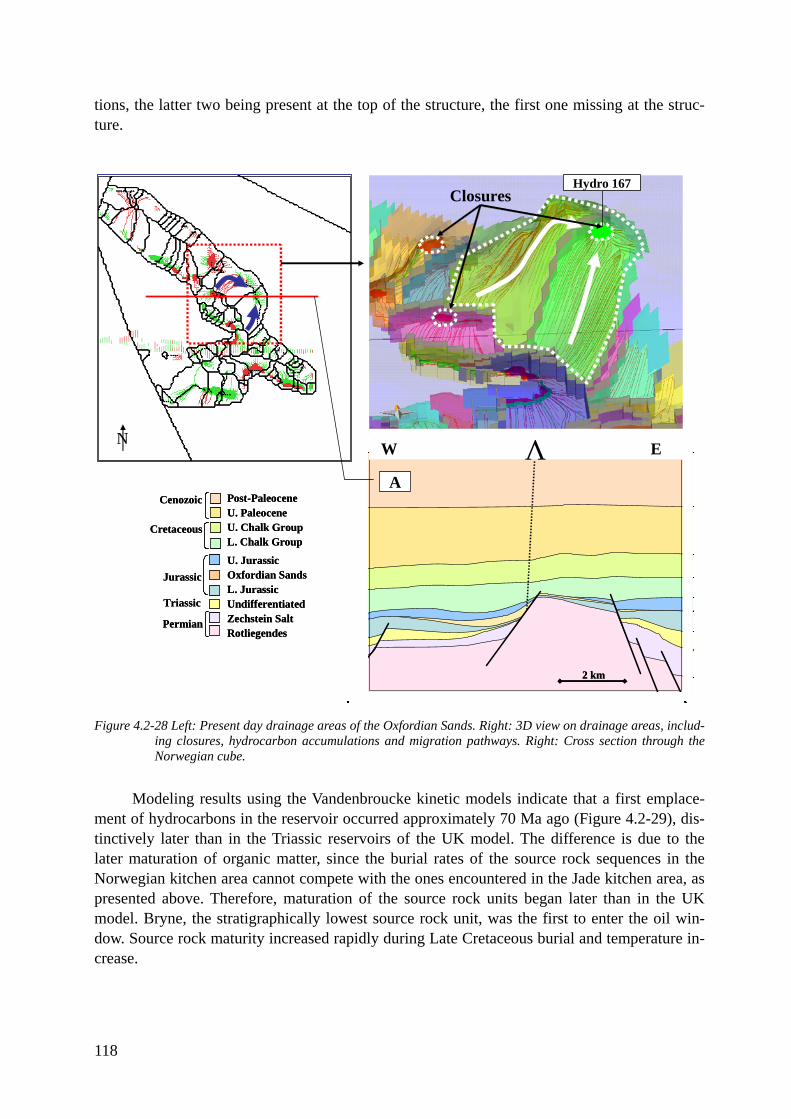
118

tions, the latter two being present at the top of the structure, the first one missing at the struc-ture.

2 km2 km2 km

W E

2 km2 km2 km

W E

Post-PaleoceneU. PaleoceneU. Chalk GroupL. Chalk Group

Cretaceous

Cenozoic

U. JurassicOxfordian SandsL. JurassicUndifferentiatedZechstein SaltRotliegendes

Permian

Jurassic

Triassic

Post-PaleoceneU. PaleoceneU. Chalk GroupL. Chalk Group

Cretaceous

Cenozoic

U. JurassicOxfordian SandsL. JurassicUndifferentiatedZechstein SaltRotliegendes

Permian

Jurassic

Triassic

Hydro 167Closures

N

A

W E

V

Figure 4.2-28 Left: Present day drainage areas of the Oxfordian Sands. Right: 3D view on drainage areas, includ-ing closures, hydrocarbon accumulations and migration pathways. Right: Cross section through the Norwegian cube.

Modeling results using the Vandenbroucke kinetic models indicate that a first emplace-ment of hydrocarbons in the reservoir occurred approximately 70 Ma ago (Figure 4.2-29), dis-tinctively later than in the Triassic reservoirs of the UK model. The difference is due to the later maturation of organic matter, since the burial rates of the source rock sequences in the Norwegian kitchen area cannot compete with the ones encountered in the Jade kitchen area, as presented above. Therefore, maturation of the source rock units began later than in the UK model. Bryne, the stratigraphically lowest source rock unit, was the first to enter the oil win-dow. Source rock maturity increased rapidly during Late Cretaceous burial and temperature in-crease.

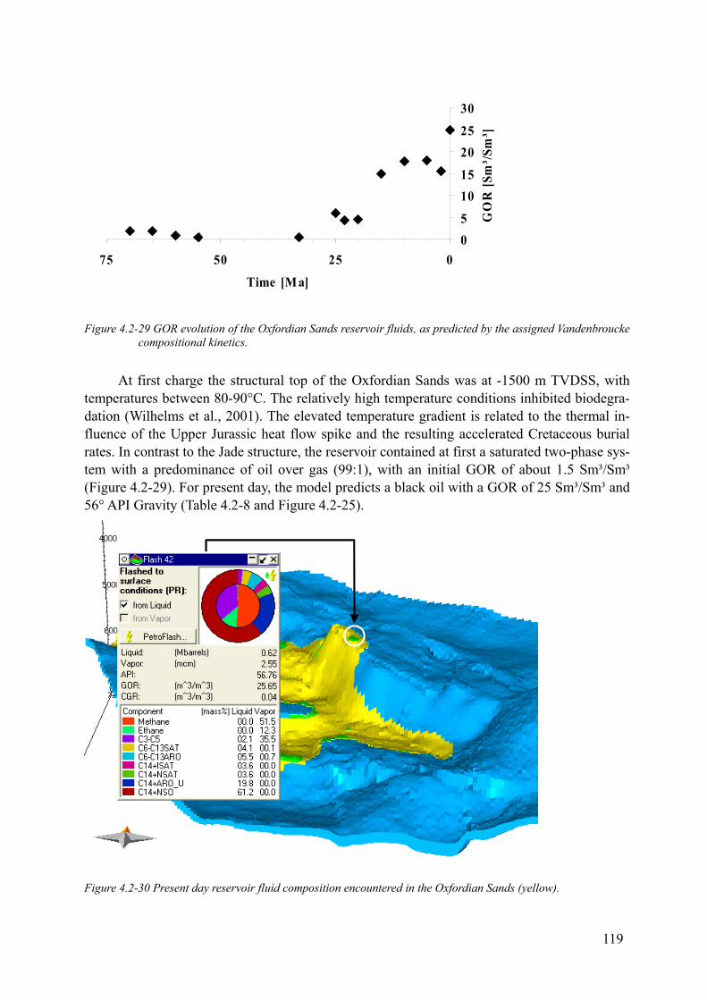
05

1015

2025

30

0255075

Time [M a]

GO

R [S

m³/S

m³]

Figure 4.2-29 GOR evolution of the Oxfordian Sands reservoir fluids, as predicted by the assigned Vandenbroucke compositional kinetics.

At first charge the structural top of the Oxfordian Sands was at -1500 m TVDSS, with temperatures between 80-90°C. The relatively high temperature conditions inhibited biodegra-dation (Wilhelms et al., 2001). The elevated temperature gradient is related to the thermal in-fluence of the Upper Jurassic heat flow spike and the resulting accelerated Cretaceous burial rates. In contrast to the Jade structure, the reservoir contained at first a saturated two-phase sys-tem with a predominance of oil over gas (99:1), with an initial GOR of about 1.5 Sm³/Sm³ (Figure 4.2-29). For present day, the model predicts a black oil with a GOR of 25 Sm³/Sm³ and 56° API Gravity (Table 4.2-8 and Figure 4.2-25).

Figure 4.2-30 Present day reservoir fluid composition encountered in the Oxfordian Sands (yellow).

119

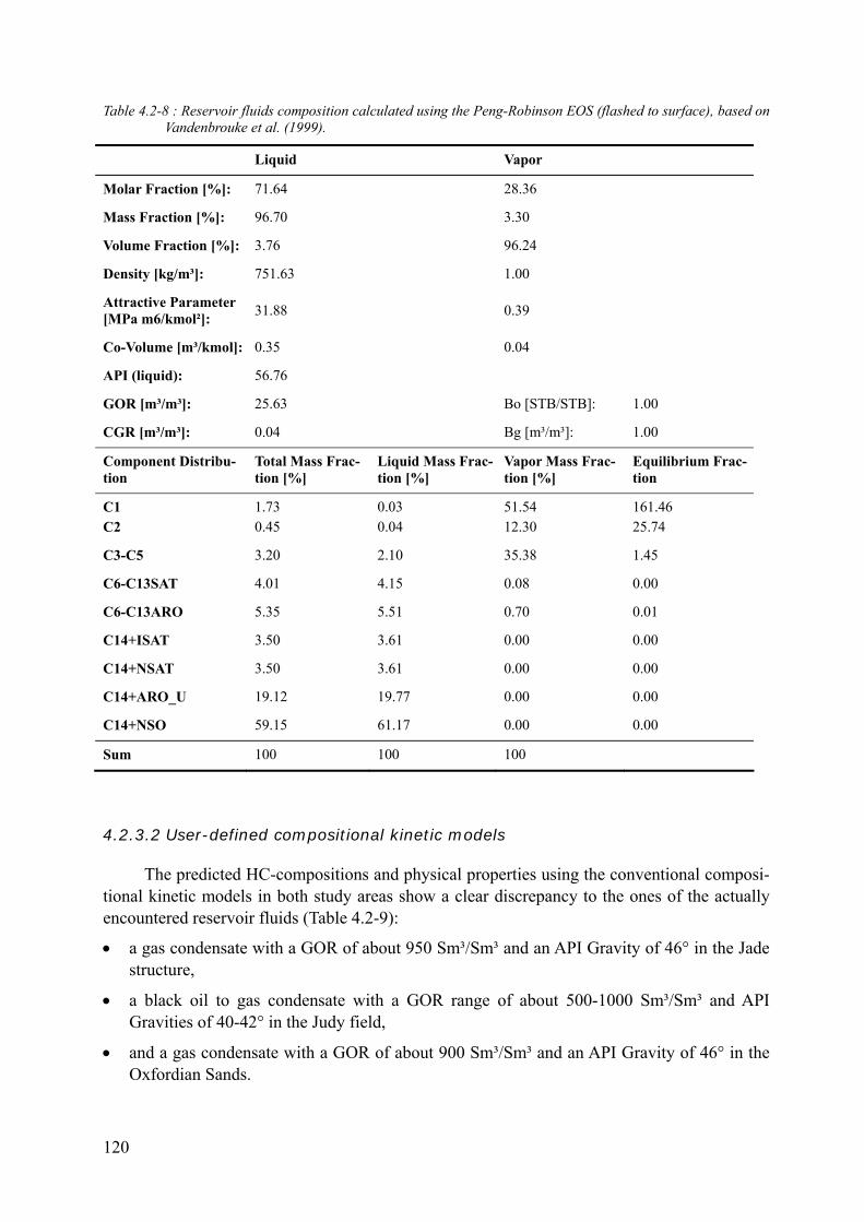
Table 4.2-8 : Reservoir fluids composition calculated using the Peng-Robinson EOS (flashed to surface), based on Vandenbrouke et al. (1999).

Liquid Vapor

Molar Fraction [%]: 71.64 28.36

Mass Fraction [%]: 96.70 3.30

Volume Fraction [%]: 3.76 96.24

Density [kg/m³]: 751.63 1.00

Attractive Parameter [MPa m6/kmol²]: 31.88 0.39

Co-Volume [m³/kmol]: 0.35 0.04

API (liquid): 56.76

GOR [m³/m³]: 25.63 Bo [STB/STB]: 1.00

CGR [m³/m³]: 0.04 Bg [m³/m³]: 1.00

Component Distribu-tion

Total Mass Frac-tion [%]

Liquid Mass Frac-tion [%]

Vapor Mass Frac-tion [%]

Equilibrium Frac-tion

C1 1.73 0.03 51.54 161.46 C2 0.45 0.04 12.30 25.74

C3-C5 3.20 2.10 35.38 1.45

C6-C13SAT 4.01 4.15 0.08 0.00

C6-C13ARO 5.35 5.51 0.70 0.01

C14+ISAT 3.50 3.61 0.00 0.00

C14+NSAT 3.50 3.61 0.00 0.00

C14+ARO_U 19.12 19.77 0.00 0.00

C14+NSO 59.15 61.17 0.00 0.00

Sum 100 100 100

4.2.3.2 User-defined compositional kinetic models

The predicted HC-compositions and physical properties using the conventional composi-tional kinetic models in both study areas show a clear discrepancy to the ones of the actually encountered reservoir fluids (Table 4.2-9):

• a gas condensate with a GOR of about 950 Sm³/Sm³ and an API Gravity of 46° in the Jade structure,

• a black oil to gas condensate with a GOR range of about 500-1000 Sm³/Sm³ and API Gravities of 40-42° in the Judy field,

• and a gas condensate with a GOR of about 900 Sm³/Sm³ and an API Gravity of 46° in the Oxfordian Sands.

120

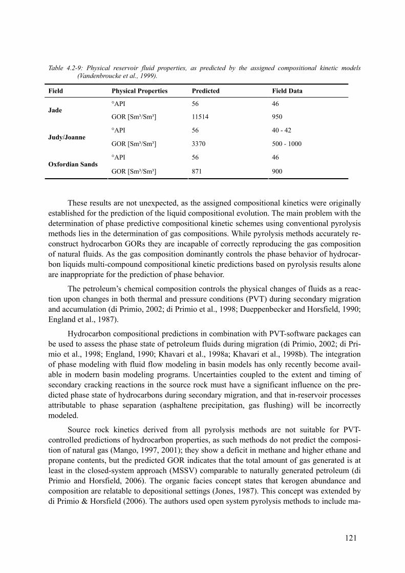
Table 4.2-9: Physical reservoir fluid properties, as predicted by the assigned compositional kinetic models (Vandenbroucke et al., 1999).

Field Physical Properties Predicted Field Data

°API 56 46 Jade

GOR [Sm³/Sm³] 11514 950

°API 56 40 - 42 Judy/Joanne

GOR [Sm³/Sm³] 3370 500 - 1000

°API 56 46 Oxfordian Sands

GOR [Sm³/Sm³] 871 900

These results are not unexpected, as the assigned compositional kinetics were originally established for the prediction of the liquid compositional evolution. The main problem with the determination of phase predictive compositional kinetic schemes using conventional pyrolysis methods lies in the determination of gas compositions. While pyrolysis methods accurately re-construct hydrocarbon GORs they are incapable of correctly reproducing the gas composition of natural fluids. As the gas composition dominantly controls the phase behavior of hydrocar-bon liquids multi-compound compositional kinetic predictions based on pyrolysis results alone are inappropriate for the prediction of phase behavior.

The petroleum’s chemical composition controls the physical changes of fluids as a reac-tion upon changes in both thermal and pressure conditions (PVT) during secondary migration and accumulation (di Primio, 2002; di Primio et al., 1998; Dueppenbecker and Horsfield, 1990; England et al., 1987).

Hydrocarbon compositional predictions in combination with PVT-software packages can be used to assess the phase state of petroleum fluids during migration (di Primio, 2002; di Pri-mio et al., 1998; England, 1990; Khavari et al., 1998a; Khavari et al., 1998b). The integration of phase modeling with fluid flow modeling in basin models has only recently become avail-able in modern basin modeling programs. Uncertainties coupled to the extent and timing of secondary cracking reactions in the source rock must have a significant influence on the pre-dicted phase state of hydrocarbons during secondary migration, and that in-reservoir processes attributable to phase separation (asphaltene precipitation, gas flushing) will be incorrectly modeled.

Source rock kinetics derived from all pyrolysis methods are not suitable for PVT-controlled predictions of hydrocarbon properties, as such methods do not predict the composi-tion of natural gas (Mango, 1997, 2001); they show a deficit in methane and higher ethane and propane contents, but the predicted GOR indicates that the total amount of gas generated is at least in the closed-system approach (MSSV) comparable to naturally generated petroleum (di Primio and Horsfield, 2006). The organic facies concept states that kerogen abundance and composition are relatable to depositional settings (Jones, 1987). This concept was extended by di Primio & Horsfield (2006). The authors used open system pyrolysis methods to include ma-

121

jor petroleum types whose gross compositions are defined by source rock kerogen and petro-leum composition which directly control the behavior of the fluids upon thermal stress. Their method allows the characterization of the compositional evolution of the fluids generated as a function of increasing thermal stress and pressure changes during secondary migration. The analytically determined gas compositions are iteratively corrected to natural fluid phase behav-ior and the ensuing corrected gas compositions are used for the definition of multi-compound kinetic models. The liquid composition only plays a minor role in phase prediction, as its im-portance lies more in the determination of fluid properties like API gravities.

A correction of only the pyrolysates gas phase composition and not of the total amount of gas is required in order to predict the phase behavior correctly. Methane is by far the most abundant compound of the gas phase in natural petroleum, having also the strongest influence on the phase behavior of the fluid, in particular on the saturation pressure. The effects are shown in Figure 4.2-32, demonstrating the error margin of using compositional data based on pyrolysis experiments for phase predictions.

The starting point for the definition of the kinetic dataset to use was based on source rock depositional environment. The PhaseKinetics approach of di Primio and Horsfield (2006) al-lows selecting specific kinetics for source rocks based on their depositional environment and the petroleum type they generate. For the Mandal/Kimmeridge sequence the Kimmeridge Clay PhaseKinetic model of di Primio and Horsfield (2006) was used. For the Bryne/Pentland for-mation, default compositional kinetics from the PhaseKinetics database of di Primio and Hors-field (2006) representative of kerogen deposited in a marine/deltaic environment was used (BH 393 Tertiary Coal). The compositional kinetic models are shown in Figure 4.2-31 and in ap-pendix II). The Farsund/Heather interval was assigned the bulk kinetic properties determined by Erdmann (1999) on a sample from that formation. Compositional information required for phase kinetics was obtained from the closed system pyrolysis experiments performed on the same sample by Erdmann (1999). Integration of the bulk kinetic and compositional data was performed following the procedure described by di Primio and Horsfield (2006).

122

Mandal/Kimmeridge Clay

0

100

200

300

400

47 49 51 53 55 57 59 61 63 65 67 69 71

Pote

ntia

l

Bryne/Pentland

0

100

200

300

47 50 53 56 59 62 65 68

Activation Energy [kcal/mol]

Pote

ntia

l

C 7+n-Hexanen-Pentanei-Pentanen-Butanei-ButanePropaneEthaneMethane

Farsund/Heather

0

100

200

300

55 56 57 58 59 60 61 62 63 64 65 66

Pote

ntia

l

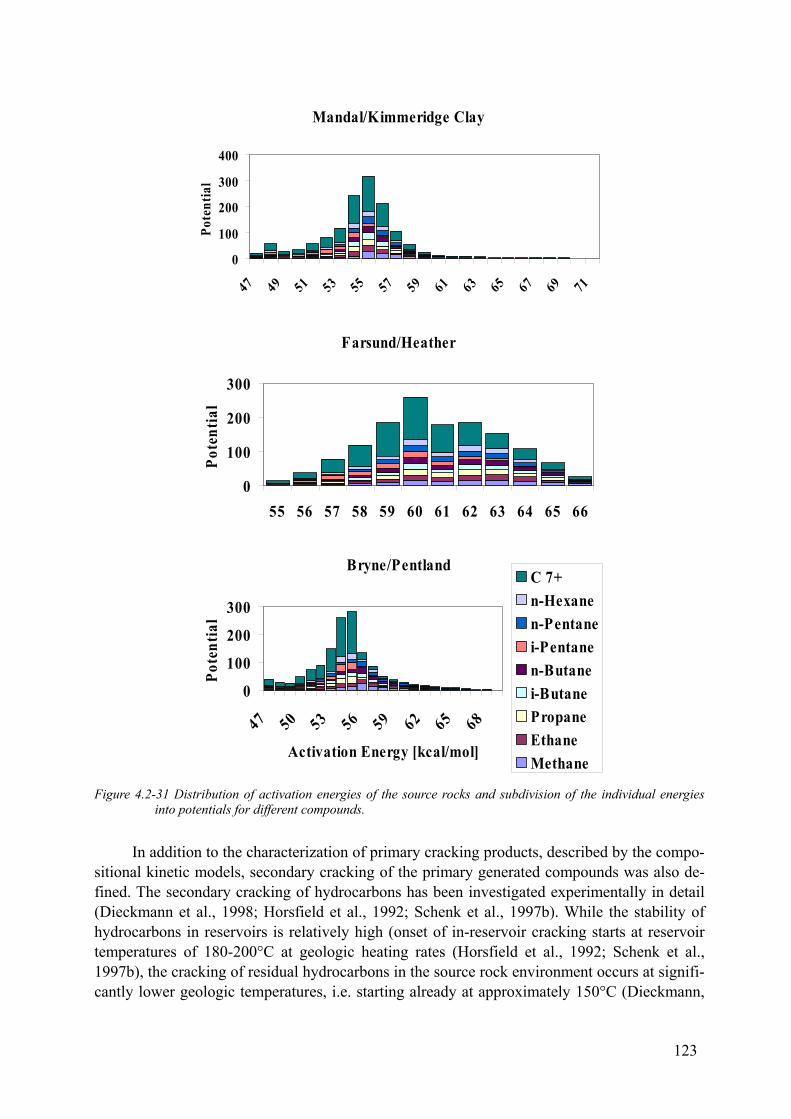
Mandal/Kimmeridge Clay

0

100

200

300

400

47 49 51 53 55 57 59 61 63 65 67 69 71

Pote

ntia

l

Bryne/Pentland

0

100

200

300

47 50 53 56 59 62 65 68

Activation Energy [kcal/mol]

Pote

ntia

l

C 7+n-Hexanen-Pentanei-Pentanen-Butanei-ButanePropaneEthaneMethane

Farsund/Heather

0

100

200

300

55 56 57 58 59 60 61 62 63 64 65 66

Pote

ntia

l

Figure 4.2-31 Distribution of activation energies of the source rocks and subdivision of the individual energies

into potentials for different compounds.

In addition to the characterization of primary cracking products, described by the compo-sitional kinetic models, secondary cracking of the primary generated compounds was also de-fined. The secondary cracking of hydrocarbons has been investigated experimentally in detail (Dieckmann et al., 1998; Horsfield et al., 1992; Schenk et al., 1997b). While the stability of hydrocarbons in reservoirs is relatively high (onset of in-reservoir cracking starts at reservoir temperatures of 180-200°C at geologic heating rates (Horsfield et al., 1992; Schenk et al., 1997b), the cracking of residual hydrocarbons in the source rock environment occurs at signifi-cantly lower geologic temperatures, i.e. starting already at approximately 150°C (Dieckmann,

123

124

2005). In the experimental studies listed, oil cracking was described by the formation of gas (C1-5) due to the cracking of the C6+ petroleum fraction. For the compositional kinetic models applied in this study, the use of 7 compounds describing the liquid composition precluded the definition of oil cracking using a single bulk reaction characterization.

The amount of gas generated by secondary cracking depends on the proportion of oil cracked to gas as well as the proportion of that fraction converted to pyrobitumen. Dieckmann et al. (1998) calculated a conversion factor of 0.7 (i.e. 70% of the cracked C6+ compounds were converted to gas and 30% to pyrobitumen) assuming average values for the H/C ratios of liquid and gaseous hydrocarbons using the following equations:

( ) nmn CHxCHxCH *1* −+=

n = average H/C-ratio of C6+ compounds m = average H/C-ratio of secondary gas u = average H/C-ratio of pyrobitumen

which yields ( )( )um

unx−−

=

and a conversion factor of ( )( )n

mxfc ++

=1212*

In these equations the following values for the variables were used:

• n = 0 2.2 (average of hexane and triacontane)

• m = 3.2 (average of methane and pentane)

• u = 0.2 (Behar et al., 1991).

Thus fc was calculated to be 0.7.

In this estimation the experimentally determined H/C ratio of the gas phase from closed system pyrolysis was used. As discussed above, the gas composition generated by any pyroly-sis method is notoriously wet. If natural gas compositions had been used in the calculations of Dieckmann et al. (1998), the H/C of the gas phase would have shifted to values approaching 4 and the total conversion factor would have decreased to 0.59.

Hantschel (pers. com. 2003) calculated an average conversion factor (termed reduction factor r in PetroMod) for oil to gas cracking of 0.57 based on the simple stoichiometry:

• 2 CH2 → 1 C + 1 CH4

• 2*14 → 12 + 16 and

• r = 16/28 = 0.57

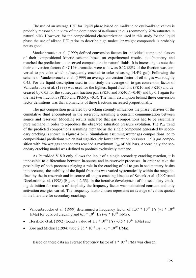
The use of an average H/C for liquid phase based on n-alkane or cyclo-alkane values is probably reasonable in view of the dominance of n-alkanes in oils (commonly 70% saturates in natural oils). However, for the compositional characterization used in this study for the liquid phase the use of alkane H/C ratios to describe high molecular weight compounds is probably not as good.

Vandenbroucke et al. (1999) defined conversion factors for individual compound classes of their compositional kinetic scheme based on experimental results, stoichiometry and matched the predictions to observed compositions in natural fluids. It is interesting to note that their conversion factors for C14+ aromatics were as low as 0.12 (88% of the fraction was con-verted to pre-coke which subsequently cracked to coke releasing 14.4% gas). Following the scheme of Vandenbroucke et al. (1999) an average conversion factor of oil to gas was roughly 0.45. For the liquid description used in this study the average oil to gas conversion factor of Vandenbrouke et al. (1999) was used for the lightest liquid fractions (PK10 and PK20) and de-creased by 0.05 for the subsequent fraction pair (PK30 and PK40 fc=0.40) and by 0.1 again for the last two fractions (PK50 and PK60 fc=0.3). The main assumption behind these conversion factor definitions was that aromaticity of these fractions increased proportionally.

The gas composition generated by cracking strongly influences the phase behavior of the cumulative fluid encountered in the reservoir, assuming a constant communication between source and reservoir. Modeling results indicated that gas compositions had to be essentially pure methane in order to reproduce the observed saturation pressure evolution. The Psat trend of the predicted compositions assuming methane as the single compound generated by secon-dary cracking is shown in Figure 4.2-32. Simulations assuming wetter gas compositions led to compositional predictions which had significantly lower saturation pressures, i.e. a gas compo-sition with 5% wet gas components reached a maximum Psat of 380 bars. Accordingly, the sec-ondary cracking model was defined to produce exclusively methane.

As PetroMod V 8.0 only allows the input of a single secondary cracking reaction, it is impossible to differentiate between in-source and in-reservoir processes. In order to take the possibility of both processes playing a role in the cracking of oil to gas in sedimentary basins into account, the stability of the liquid fractions was varied systematically within the range de-fined by the in-reservoir and in-source oil to gas cracking kinetics of Schenk et al. (1997b)and Dieckmann et al. (1998) (Figure 4.2-33). In the iterative development of the secondary crack-ing definition for reasons of simplicity the frequency factor was maintained constant and only activation energies varied. The frequency factor chosen represents an average of values quoted in the literature for secondary cracking:

• Vandenbroucke et al. (1999) determined a frequency factor of 1.37 * 1014 28 1/s (~1 * 10 1/Ma) for bulk oil cracking and 6.1 * 1017 31 1/s (~2 * 10 1/Ma),

• Horsfield et al. (1992) found a value of 1.1 * 1016 1/s (~3.5 * 1029 1/Ma) and 16• Kuo and Michael (1994) used 2.85 * 10 1/s (~1 * 1030 1/Ma).

Based on these data an average frequency factor of 1 * 1030 1/Ma was chosen.

125

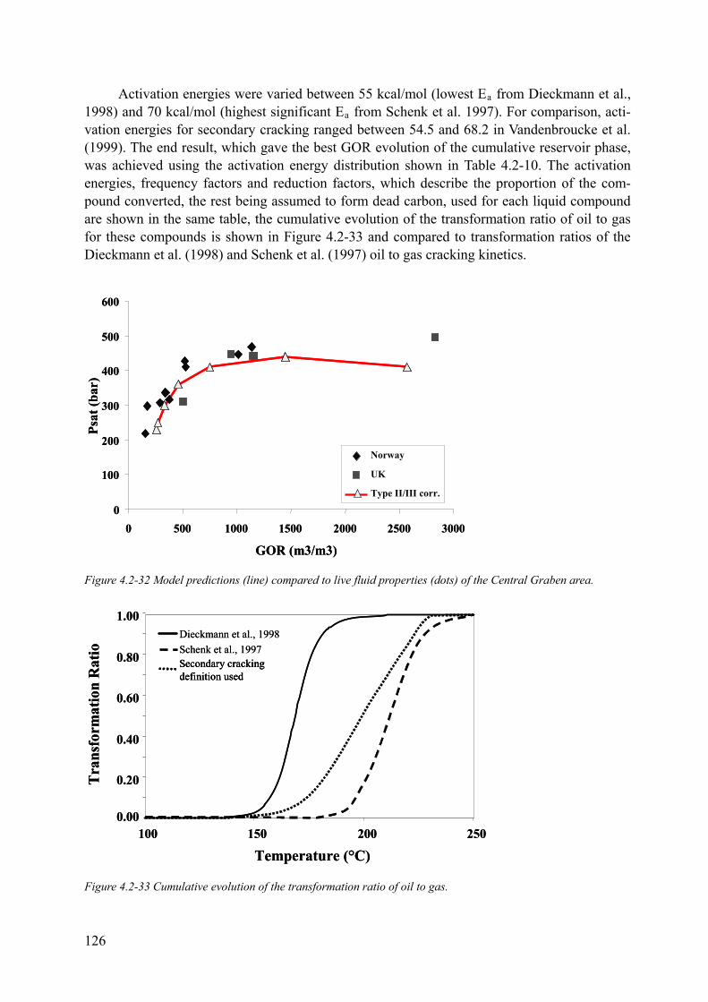
Activation energies were varied between 55 kcal/mol (lowest Ea from Dieckmann et al., 1998) and 70 kcal/mol (highest significant Ea from Schenk et al. 1997). For comparison, acti-vation energies for secondary cracking ranged between 54.5 and 68.2 in Vandenbroucke et al. (1999). The end result, which gave the best GOR evolution of the cumulative reservoir phase, was achieved using the activation energy distribution shown in Table 4.2-10. The activation energies, frequency factors and reduction factors, which describe the proportion of the com-pound converted, the rest being assumed to form dead carbon, used for each liquid compound are shown in the same table, the cumulative evolution of the transformation ratio of oil to gas for these compounds is shown in Figure 4.2-33 and compared to transformation ratios of the Dieckmann et al. (1998) and Schenk et al. (1997) oil to gas cracking kinetics.

0

100

200

300

400

500

600

0 500 1000 1500 2000 2500 3000

GOR (m3/m3)

Psat

(bar

)

Norway

UK

Type II/III corr.

0

100

200

300

400

500

600

0 500 1000 1500 2000 2500 3000

GOR (m3/m3)

Psat

(bar

)

Norway

UK

Type II/III corr.

Figure 4.2-32 Model predictions (line) compared to live fluid properties (dots) of the Central Graben area.

0.00

0.20

0.40

0.60

0.80

1.00

100 150 200 250

Temperature (°C)

Tra

nsfo

rmat

ion

Rat

io

Dieckmann et al., 1998Schenk et al., 1997Secondary crackingdefinition used

0.00

0.20

0.40

0.60

0.80

1.00

100 150 200 250

Temperature (°C)

Tra

nsfo

rmat

ion

Rat

io

Dieckmann et al., 1998Schenk et al., 1997Secondary crackingdefinition usedSecondary crackingdefinition used

Figure 4.2-33 Cumulative evolution of the transformation ratio of oil to gas.

126

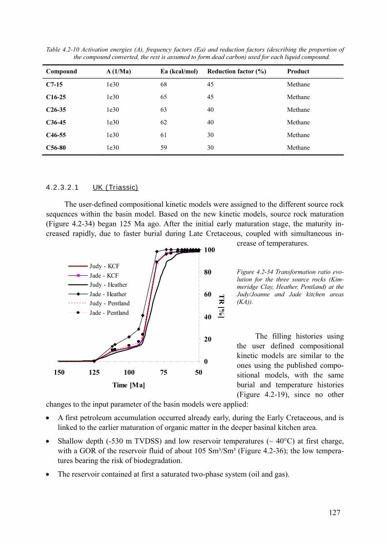
Table 4.2-10 Activation energies (A), frequency factors (Ea) and reduction factors (describing the proportion of the compound converted, the rest is assumed to form dead carbon) used for each liquid compound.

Compound A (1/Ma) Ea (kcal/mol) Reduction factor (%) Product

C7-15 1e30 68 45 Methane

C16-25 1e30 65 45 Methane

C26-35 1e30 63 40 Methane

C36-45 1e30 62 40 Methane

C46-55 1e30 61 30 Methane

C56-80 1e30 59 30 Methane

4.2.3.2.1 UK (Triassic)

The user-defined compositional kinetic models were assigned to the different source rock sequences within the basin model. Based on the new kinetic models, source rock maturation (Figure 4.2-34) began 125 Ma ago. After the initial early maturation stage, the maturity in-creased rapidly, due to faster burial during Late Cretaceous, coupled with simultaneous in-

crease of temperatures.

Figure 4.2-34 Transformation ratio evo-lution for the three source rocks (Kim-meridge Clay, Heather, Pentland) at the Judy/Joanne and Jade kitchen areas (KA)).

The filling histories using the user defined compositional kinetic models are similar to the ones using the published compo-sitional models, with the same burial and temperature histories (Figure 4.2-19), since no other

changes to the input parameter of the basin models were applied:

0

20

40

60

80

100

5075100125150

Time [Ma]

TR

[%]

Judy - KCFJade - KCFJudy - HeatherJade - HeatherJudy - PentlandJade - Pentland

• A first petroleum accumulation occurred already early, during the Early Cretaceous, and is linked to the earlier maturation of organic matter in the deeper basinal kitchen area.

• Shallow depth (-530 m TVDSS) and low reservoir temperatures (~ 40°C) at first charge, with a GOR of the reservoir fluid of about 105 Sm³/Sm³ (Figure 4.2-36); the low tempera-tures bearing the risk of biodegradation.

• The reservoir contained at first a saturated two-phase system (oil and gas).

127

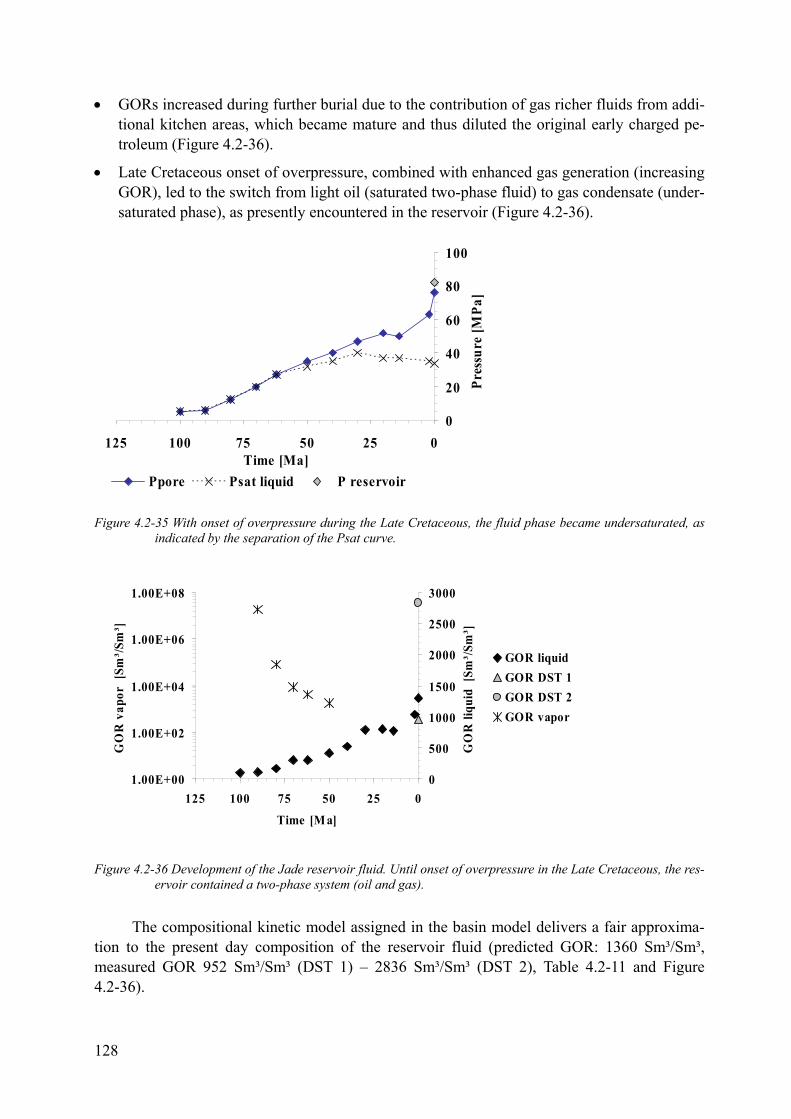
• GORs increased during further burial due to the contribution of gas richer fluids from addi-tional kitchen areas, which became mature and thus diluted the original early charged pe-troleum (Figure 4.2-36).

• Late Cretaceous onset of overpressure, combined with enhanced gas generation (increasing GOR), led to the switch from light oil (saturated two-phase fluid) to gas condensate (under-saturated phase), as presently encountered in the reservoir (Figure 4.2-36).

0

20

40

60

80

100

0255075100125Time [Ma]

Pres

sure

[MPa

]Ppore Psat liquid P reservoir

Figure 4.2-35 With onset of overpressure during the Late Cretaceous, the fluid phase became undersaturated, as indicated by the separation of the Psat curve.

0

500

1000

1500

2000

2500

3000

0255075100125

Time [M a]

GO

R li

quid

[Sm

³/Sm

³]

1.00E+00

1.00E+02

1.00E+04

1.00E+06

1.00E+08

GO

R v

apor

[Sm

³/Sm

³]

GOR liquidGOR DST 1GOR DST 2GOR vapor

Figure 4.2-36 Development of the Jade reservoir fluid. Until onset of overpressure in the Late Cretaceous, the res-ervoir contained a two-phase system (oil and gas).

The compositional kinetic model assigned in the basin model delivers a fair approxima-tion to the present day composition of the reservoir fluid (predicted GOR: 1360 Sm³/Sm³, measured GOR 952 Sm³/Sm³ (DST 1) – 2836 Sm³/Sm³ (DST 2), Table 4.2-11 and Figure 4.2-36).

128

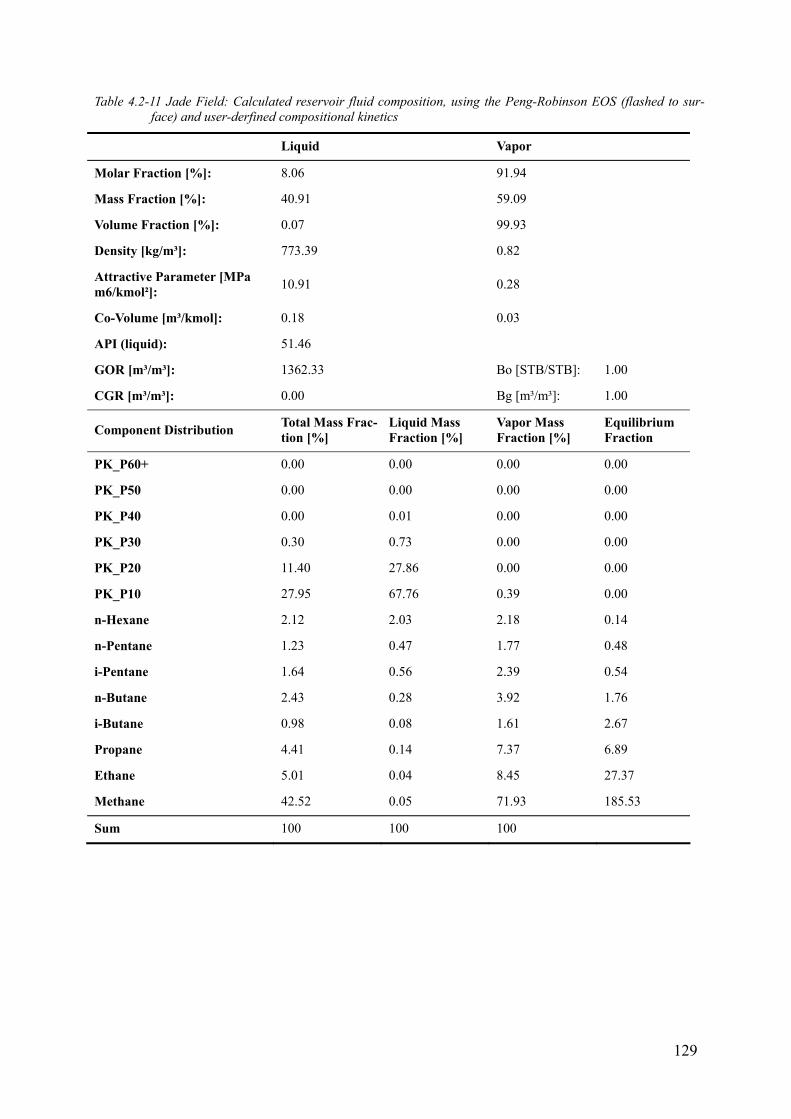
Table 4.2-11 Jade Field: Calculated reservoir fluid composition, using the Peng-Robinson EOS (flashed to sur-face) and user-derfined compositional kinetics

Liquid Vapor

Molar Fraction [%]: 8.06 91.94

Mass Fraction [%]: 40.91 59.09

Volume Fraction [%]: 0.07 99.93

Density [kg/m³]: 773.39 0.82

Attractive Parameter [MPa m6/kmol²]: 10.91 0.28

Co-Volume [m³/kmol]: 0.18 0.03

API (liquid): 51.46

GOR [m³/m³]: 1362.33 Bo [STB/STB]: 1.00

CGR [m³/m³]: 0.00 Bg [m³/m³]: 1.00

Total Mass Frac-tion [%]

Liquid Mass Fraction [%]

Vapor Mass Fraction [%]

Equilibrium Fraction Component Distribution

PK_P60+ 0.00 0.00 0.00 0.00

PK_P50 0.00 0.00 0.00 0.00

PK_P40 0.00 0.01 0.00 0.00

PK_P30 0.30 0.73 0.00 0.00

PK_P20 11.40 27.86 0.00 0.00

PK_P10 27.95 67.76 0.39 0.00

n-Hexane 2.12 2.03 2.18 0.14

n-Pentane 1.23 0.47 1.77 0.48

i-Pentane 1.64 0.56 2.39 0.54

n-Butane 2.43 0.28 3.92 1.76

i-Butane 0.98 0.08 1.61 2.67

Propane 4.41 0.14 7.37 6.89

Ethane 5.01 0.04 8.45 27.37

Methane 42.52 0.05 71.93 185.53

Sum 100 100 100

129

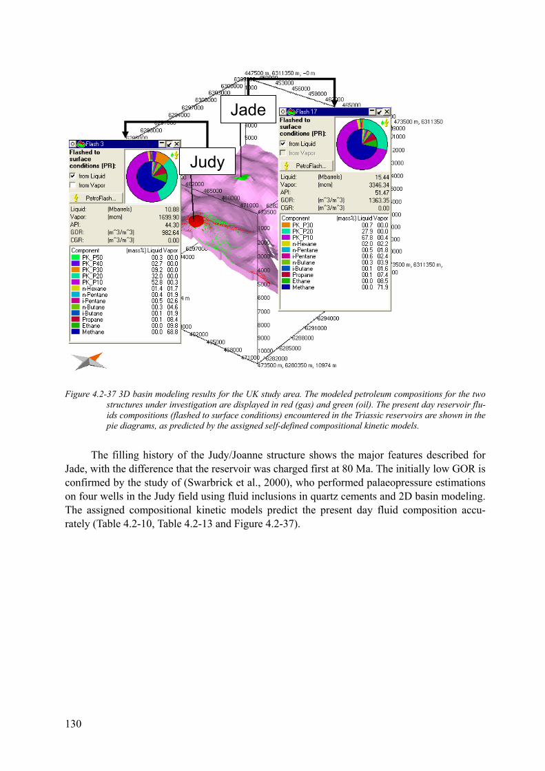
Judy

Jade

Judy

Jade

Figure 4.2-37 3D basin modeling results for the UK study area. The modeled petroleum compositions for the two structures under investigation are displayed in red (gas) and green (oil). The present day reservoir flu-ids compositions (flashed to surface conditions) encountered in the Triassic reservoirs are shown in the pie diagrams, as predicted by the assigned self-defined compositional kinetic models.

The filling history of the Judy/Joanne structure shows the major features described for Jade, with the difference that the reservoir was charged first at 80 Ma. The initially low GOR is confirmed by the study of (Swarbrick et al., 2000), who performed palaeopressure estimations on four wells in the Judy field using fluid inclusions in quartz cements and 2D basin modeling. The assigned compositional kinetic models predict the present day fluid composition accu-rately (Table 4.2-10, Table 4.2-13 and Figure 4.2-37).

130

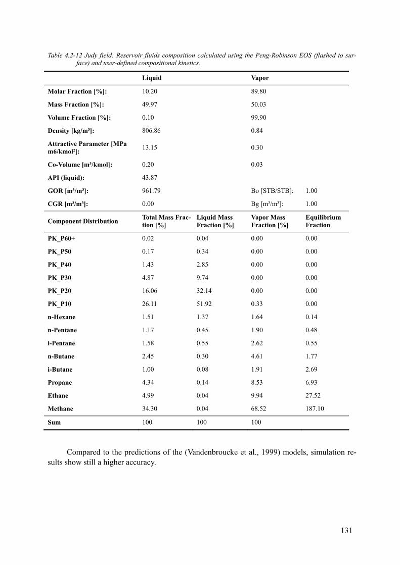
Table 4.2-12 Judy field: Reservoir fluids composition calculated using the Peng-Robinson EOS (flashed to sur-face) and user-defined compositional kinetics.

Liquid Vapor

Molar Fraction [%]: 10.20 89.80

Mass Fraction [%]: 49.97 50.03

Volume Fraction [%]: 0.10 99.90

Density [kg/m³]: 806.86 0.84

Attractive Parameter [MPa m6/kmol²]: 13.15 0.30

Co-Volume [m³/kmol]: 0.20 0.03

API (liquid): 43.87

GOR [m³/m³]: 961.79 Bo [STB/STB]: 1.00

CGR [m³/m³]: 0.00 Bg [m³/m³]: 1.00

Total Mass Frac-tion [%]

Liquid Mass Fraction [%]

Vapor Mass Fraction [%]

Equilibrium Fraction Component Distribution

PK_P60+ 0.02 0.04 0.00 0.00

PK_P50 0.17 0.34 0.00 0.00

PK_P40 1.43 2.85 0.00 0.00

PK_P30 4.87 9.74 0.00 0.00

PK_P20 16.06 32.14 0.00 0.00

PK_P10 26.11 51.92 0.33 0.00

n-Hexane 1.51 1.37 1.64 0.14

n-Pentane 1.17 0.45 1.90 0.48

i-Pentane 1.58 0.55 2.62 0.55

n-Butane 2.45 0.30 4.61 1.77

i-Butane 1.00 0.08 1.91 2.69

Propane 4.34 0.14 8.53 6.93

Ethane 4.99 0.04 9.94 27.52

Methane 34.30 0.04 68.52 187.10

Sum 100 100 100

Compared to the predictions of the (Vandenbroucke et al., 1999) models, simulation re-sults show still a higher accuracy.

131

4.2.3.2.2 Norway (Jurassic)

Again, the new compositional kinetic models were assigned to the different source rock sequences within the basin model. No other changes to the input parameter of the basin models were applied. The results showed, that

• the Bryne formation was the first to enter the oil window, at approximately 80 Ma (Figure 4.2-38).

• A first petroleum accumulation occurred in the upper Late Cretaceous already early, during the Early Cretaceous, and is linked to the earlier maturation of organic matter in the deeper basinal kitchen area.

• Deeper burial depth than Jade (-1500 m TVDSS) and relatively high reservoir temperatures (80-90°C) at first charge (Figure 4.2-41).

• The reservoir contained at first a saturated two-phase system (oil and gas), with an initial GOR of the of the oil phase of about 200 Sm³/Sm³, and a GOR of the gas phase of about 6000 Sm³/Sm³ (Figure 4.2-40).

• GORs increased during further burial due to the contribution of gas richer fluids from addi-tional kitchen areas, which became mature and thus diluted the original early charged pe-troleum (Figure 4.2-40).

• Late Cretaceous onset of overpressure (Figure 4.2-41) is associated with enhanced gas gen-eration (increasing GOR), and led to the switch from light oil (saturated two-phase fluid) to gas condensate (undersaturated phase), as presently encountered in the reservoir (Figure 4.2-42).

• These fluids increased in GOR during further source rock maturation due to the contribu-tion of gas richer fluids, which diluted the original early charged petroleum.

• The compositional kinetic models assigned in the basin model deliver a prediction which matches the present day composition of the reservoir fluids and their physical properties (predicted GOR: 871 Sm³/Sm³, field data: 900 Sm³/Sm³; predicted API gravity 45°, field data: 46° API, Table 4.2-13 and Figure 4.2-42).

132

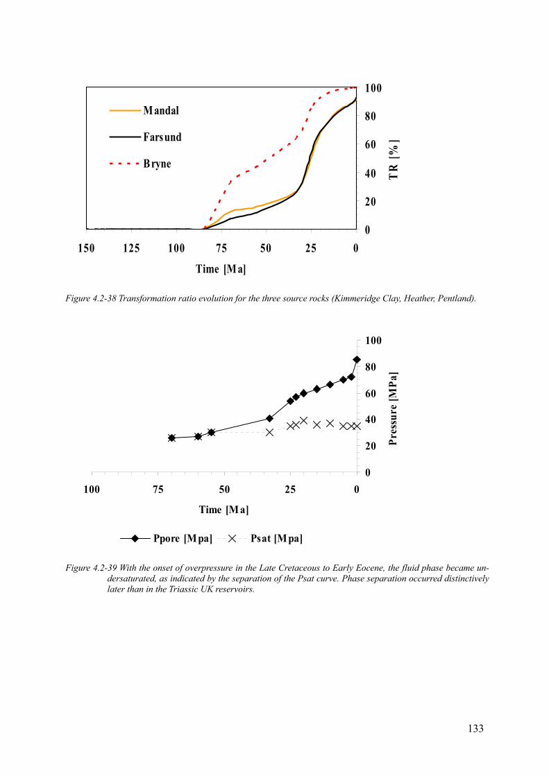
0

20

40

60

80

100

0255075100125150

Time [Ma]

TR

[%]

Mandal

Farsund

Bryne

Figure 4.2-38 Transformation ratio evolution for the three source rocks (Kimmeridge Clay, Heather, Pentland).

0

20

40

60

80

100

0255075100

Time [Ma]

Pres

sure

[MPa

]

Ppore [Mpa] Psat [Mpa]

Figure 4.2-39 With the onset of overpressure in the Late Cretaceous to Early Eocene, the fluid phase became un-dersaturated, as indicated by the separation of the Psat curve. Phase separation occurred distinctively later than in the Triassic UK reservoirs.

133

0

200

400

600

800

1000

0255075100

Time [Ma]

GO

R li

quid

[Sm

³/Sm

³]

0

2000

4000

6000

8000

10000G

OR

vap

or [S

m³/S

m³]

GOR liquidGOR FieldGOR vapor

Figure 4.2-40 GOR development in the Oxfordian sands. The increase of the GOR of the fluids is linked to accel-erated burial, coupled with further source rock maturation.

0

10

20

30

40

50

0255075100125150

Time [Ma]

Pres

sure

[Exc

ess H

ydra

ulic

, MPa

]

Combined Model Disequilibrium Compaction

0

50

100

150

200

0255075100125150

Time [Ma]

Pres

sure

[Exc

ess H

ydra

ulic

, M

Pa]

0

500

1000

1500

2000

2500

3000

3500

4000

4500

Dep

th [m

]

Temperature Depth

First Charge

0

10

20

30

40

50

0255075100125150

Time [Ma]

Pres

sure

[Exc

ess H

ydra

ulic

, MPa

]

Combined Model Disequilibrium Compaction

0

50

100

150

200

0255075100125150

Time [Ma]

Pres

sure

[Exc

ess H

ydra

ulic

, M

Pa]

0

500

1000

1500

2000

2500

3000

3500

4000

4500

Dep

th [m

]

Temperature Depth

First Charge

Figure 4.2-41 In the Norwegian Oxfordian reservoirs temperatures above 80°C at first fluid emplacement pre-cluded the risk of significant biodegradation.

134

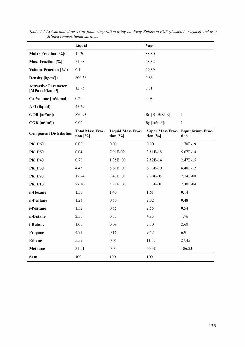
Table 4.2-13 Calculated reservoir fluid composition using the Peng-Robinson EOS (flashed to surface) and user-defined compositional kinetics.

Liquid Vapor

Molar Fraction [%]: 11.20 88.80

Mass Fraction [%]: 51.68 48.32

Volume Fraction [%]: 0.11 99.89

Density [kg/m³]: 800.38 0.86

Attractive Parameter [MPa m6/kmol²]: 12.95 0.31

Co-Volume [m³/kmol]: 0.20 0.03

API (liquid): 45.29

GOR [m³/m³]: 870.93 Bo [STB/STB]: 1

CGR [m³/m³]: 0.00 Bg [m³/m³]: 1

Total Mass Frac-tion [%]

Liquid Mass Frac-tion [%]

Vapor Mass Frac-tion [%]

Equilibrium Frac-tion Component Distribution

PK_P60+ 0.00 0.00 0.00 1.70E-19

PK_P50 0.04 7.91E-02 3.81E-18 5.67E-18

PK_P40 0.70 1.35E+00 2.82E-14 2.47E-15

PK_P30 4.45 8.61E+00 6.13E-10 8.40E-12

PK_P20 17.94 3.47E+01 2.28E-05 7.74E-08

PK_P10 27.10 5.21E+01 3.23E-01 7.30E-04

n-Hexane 1.50 1.40 1.61 0.14

n-Pentane 1.23 0.50 2.02 0.48

i-Pentane 1.52 0.55 2.55 0.54

n-Butane 2.55 0.33 4.93 1.76

i-Butane 1.06 0.09 2.10 2.68

Propane 4.71 0.16 9.57 6.91

Ethane 5.59 0.05 11.52 27.45

Methane 31.61 0.04 65.38 186.23

Sum 100 100 100

135

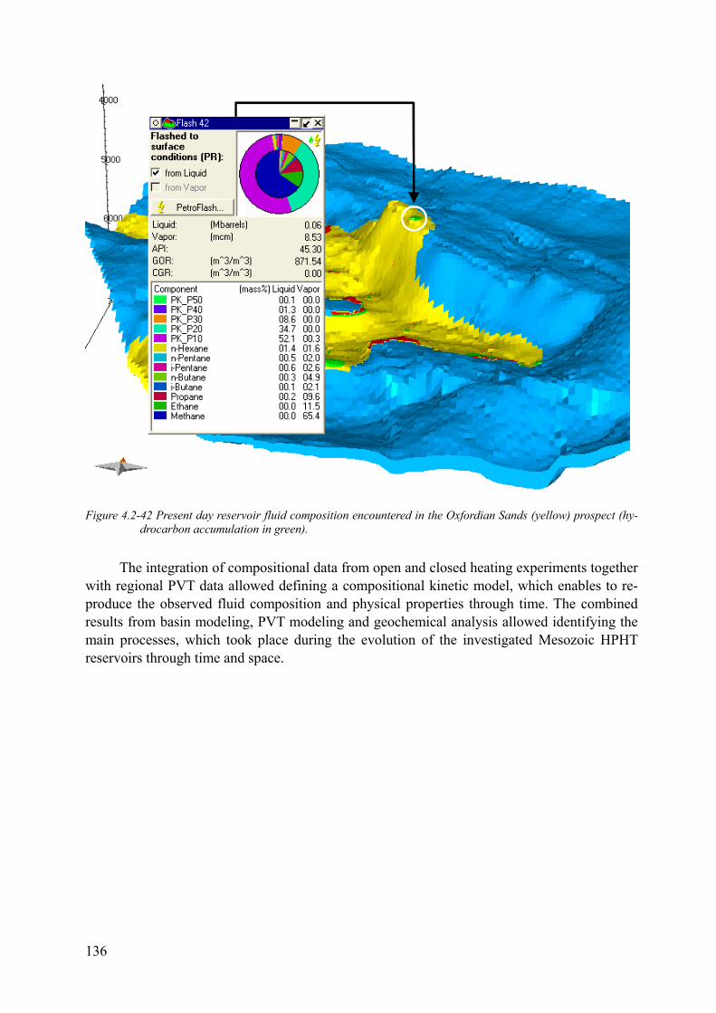
Figure 4.2-42 Present day reservoir fluid composition encountered in the Oxfordian Sands (yellow) prospect (hy-drocarbon accumulation in green).

The integration of compositional data from open and closed heating experiments together with regional PVT data allowed defining a compositional kinetic model, which enables to re-produce the observed fluid composition and physical properties through time. The combined results from basin modeling, PVT modeling and geochemical analysis allowed identifying the main processes, which took place during the evolution of the investigated Mesozoic HPHT reservoirs through time and space.

136

5 Discussion

The main goals of this study were to investigate the processes leading to the establish-ment of HPHT conditions in deep sedimentary basins as well as their effect on the hydrocar-bons accumulating in reservoirs. In detail the focus was on investigating

• heat flow history,

• pressure evolution and its numerical reproduction, and

• the reproduction of the hydrocarbon compositional evolution in the deep Mesozoic HPHT reservoirs of the Central Graben and its evolution through time.

This was achieved using

• geological and geochemical analysis,

• 3D basin modeling, and

• tuning compositional kinetic models for the main source rock sequences.

The previous chapters of this study gave an overview of the key literature available to date, the data used and the results obtained. The geological setting studied is centered on the UK and Norwegian Central Graben, an area well known for the HPHT conditions existing in its deepest regions. The common occurrence of wet gas condensates in this environment was addressed in this study by means of an advanced kinetic modeling approach. The term inverse modeling is used here to describe the methodology of reconstructing fluid compositional evo-lution by combining open and closed system pyrolysis results. Petroleum compositions derived from pyrolysis experiments are very accurate with respect to the oil range compounds; it’s the reproduced gas composition which is too wet and requires therefore a correction, which is cur-rently empirical in the PhaseKinetic approach of di Primio and Horsfield (2006).

The compositional kinetic models used in this context were:

• For the Kimmeridge Clay/Draupne formation the PhaseKinetic model developed by di Primio and Horsfield (2006) was used.

• For the main source of the HPHT reservoirs, the Heather/Farsund formation a composi-tional kinetic model was developed following the PhaseKinetic approach

• For the Pentland/Bryne formation a compositional model was selected based on source rock organogfacies. Here a kinetic model corresponding to a marine/deltaic source rock type was selected.

In all cases secondary cracking reactions were simulated using a kinetic model specifi-cally tuned to match the observed GOR and Psat evolution of high maturity fluids, but based on published activation energy, frequency factor and conversion factor ranges.

137

The result of this exercise was a pragmatic (as opposed to deterministic) approach to compositional modeling, allowing a better understanding of where the compositional or expul-sion models require more work.

Simulation results indicated that the main product of oil to gas cracking must be meth-ane, as a wetter gas compositions led to suppressed saturation pressure values. These results indicate that the too-wet gas compositions generated by pyrolysis also predominate in the com-positions of products generated by secondary cracking. With respect to the dominant control on reservoir fluid composition at elevated temperatures, the results point out that reactions occur-ring within the source rock define the composition of the reservoir fluid.

In general it can be stated that in-reservoir processes were of subordinate relevance in the cases investigated in this study, where the main kitchen areas were always deeper and hotter than the reservoirs. The main conclusions drawn from this study with respect to in-source vs. in-reservoir cracking were furthermore supported by geochemical analyses and PVT data as discussed below.

The organic geochemical evidence found in the extracted organic matter of the cored res-ervoir interval and the two DST samples indicate that the reservoir fluid encountered in the Jade structure has experienced already a high level of thermal maturation. A detectable retarda-tion of maturation was not observed. The n-alkane distributions of the two gas condensates tested in the two DST’s from GC analysis displayed in Figure 3.2-2 show high levels of ther-mal maturity. The molecular parameters frequently used for the assessment of the thermal ma-turity from GC-MS analyses of aliphatic compounds from the core extracts (steranes and ho-panes) show that the gas condensates encountered in the Jade well 30/2c-4 has already reached a high level of thermal maturity. Furthermore, the Pr/Ph and isoprenoid/n-alkane ratios found, as well as the CPI, indicate also a non-biodegraded oil to be present in the Jade structure, which originated from a mixed Type II to Type II/III kerogen organic source facies (higher land plants and algal). The high maturity shown in the two Jade condensates is consistent with the high modeled maturity of the main kitchen area. Since the two samples received from the DST’s taken directly above and only slightly below the cored section of the well resemble strongly the typical reservoir fluids in the area, which are predominantly generated in the Kimmeridge Clay and Heather Formation while the Pentland Formation is only of local impor-tance, it is reasonable to assume that the reservoir fluids originated from the same source rocks.

The different GOR’s encountered in the two DST’s indicate compartmentalization within the reservoir. Here, evidence was found within the mono vs. tri-aromatic steroid ratios of the two samples, as well as in the calculated Pressure- and GOR depth trends, using the PVT mod-eling software package PVT Sim Vs. 13.1. Both point towards reservoir compartmentalization, with the upper section as the recipient of the last charge with a more mature, in the source rock thermally cracked fluid. The latter conclusion is drawn from the observations that both fluids still contain large proportions of waxes and that the liquid fractions are characterized by com-paratively low API gravities for gas condensates.

The correct prediction of hydrocarbon phase and composition depends significantly on the pressure and temperature evolution of the carrier and reservoir system, as phase separation and differential migration of oil and gas are controlled by both the composition of the fluids and the respective pT conditions during migration and accumulation. Accordingly, the assess-

138

ment of the thermal history of the basin and the simulation of overpressure development and magnitude in the system was of critical importance.

A variety of published thermal histories, all following different philosophies, were tested. The thermal maturity data are in agreement with the rifting heat flow model of McKenzie (1980). However, thermal modeling does not show the necessity to use crustal stretching model of Mackenzie, as constant heat flow leads to identical results. That means that the amplitude and the timing of rifting are of minor importance, as long as the source rock is presently at its maximum burial depth. This outcome confirms the results published in the study of Hermanrud (1993).

Present day overpressure is generally assumed to be associated to both gas generation and disequilibrium compaction, especially during the youngest burial event of the basin stud-ied. The frequently reported retardation of maturity in overpressured sediments was only ob-served in one well, whereby the vast majority of calibration wells showed no retardation ef-fects.

While most published work relates overpressure generation to either disequilibrium compaction or gas generation, the methods used to reach these conclusions are generally unsat-isfactory. For example, Swarbrick et al. (1998) used 2D basin modeling in combination with fluid inclusion studies to conclude that overpressure generation in the same study area as inves-tigated here was dominantly controlled by disequilibrium compaction. Isaksen (2004) con-cluded in his investigation of the evolution of the Central Graben, that overpressure was mainly related to gas generation. His conclusions were, however, drawn from a correlation of over-pressure with enhanced in-situ temperatures. These two examples demonstrate the lack of a systematic test of the effects of different mechanisms on the total overpressure generated. The results of this study indicate that for the numerical reproduction of the encountered pressure conditions, none of the main pressure generation mechanisms can be exclusively favored, al-though both main mechanisms (lateral pressure transfer is implicitly included in 3D basin modeling) allow an accurate reproduction of the pressure settings. The permeabilities neces-sary to preserve overpressure generated only by disequilibrium compaction below the sealing chalks over geological times are 10-9 mD and less, values almost unlikely low to appear in natural chalks. On the contrary, overpressure generated by gas generation alone is possible to model, but unreasonable amounts and properties of the generated gas have to be assumed in natural sedimentary basins.

The approach used here to model overpressure generation focuses on a combined model, which includes gas generation, mechanical compaction and lateral pressure transfer. The key control on the effect of gas volumes generated on the overpressure evolution is its compressi-bility. Using a variety of methods, gas compressibility was determined based on the observed gas compositions in the basin. Assuming that the reproduction of present day pore pressures in the 3D models indicates that the pressure controlling mechanisms are simulated correctly, and that since the pressure seal evolution allowed the correct pressure prediction for the carriers at different depths and in different structural situations in the models, the statement that pressure evolution was modeled more or less correctly is defendable. In addition, whether the pore pres-sure increase is due to either mechanical or temperature controlled processes, or a combination of both, the main control can be simplified to enhanced burial rates where both variables in-crease. In the modeled pore pressure evolution a clear link between rapid burial and pore pres-

139

sure increase is seen, whereby significant pressure increase occurs mainly for the latest, fastest burial event.

However, the combination of gas generation and disequilibrium compaction correctly re-produced the palaeo-pT conditions of Judy Field as reported by Swarbrick et al. (2000) based on fluid inclusion confocal microscopy combined with PVT modeling. Also fluid inclusion GORs were correctly predicted by the 3D model for the time of inclusion formation. In essence all the evidence available indicates that the overpressure calculations are realistic and probably closely reproduce the natural processes.

Using this combination of disequilibrium compaction and gas generation, a series of side effects with respect to the fluid flow in the system become evident: Where extremely low cap rock permeabilities are used in order to match present day pressures using disequilibrium com-paction alone, hydrocarbon flow in the model tends to reach the cap rock and is then diverted laterally below the cap surface. This leads to a general loss of migrating hydrocarbons out the sides of the model. When gas generation is additionally taken into account, cap rock perme-abilities have to be increased. Accordingly leakage of hydrocarbons through the cap rock be-comes more prominent, a fact which is supported by observations of gas chimneys above struc-tural highs going through the chalks and Cenozoic sequences. In general the higher permeabili-ties used in the combined approach seem to be more realistic.

Interestingly, in all cases modeled it was only the increase in overpressure that was re-sponsible for the undersaturation of the reservoir fluids. During the early history of the reser-voirs, hydrocarbons occurred as two phase systems, whereby the proportion of gas was highest at the shallowest and coolest positions. In both the Triassic and Oxfordian reservoir sequences investigated, the main hydrocarbon charge came from the Farsund/Heather, and only minor proportions from the Pentland/Bryne formations. The Upper Jurassic Kimmeridge Clay/Mandal formation did not contribute significantly to the accumulations in the modeling results (which, in the reservoirs studied were predominantly in older stratigraphic layers). The gas condensates in these reservoirs today are, hence, the product of a terrestrially influenced source rock type, combined with enhanced levels of maturity extending into the early secon-dary oil-cracking zone. This latter statement is based on the observation, that the compositional descriptions of the reservoir fluids in the 3D models show that the highest molecular weight compounds (C36-C80) have already cracked to gas, a modeling result which is corroborated by the low average molecular weight of the liquid fraction of the natural fluids tested in these fields (data from PVT reports). Here it is interesting to note, that the secondary cracking kinet-ics which allowed such a good match of observed reservoir fluid compositions and physical properties actually represent a mixture of the two extremes of cracking kinetics reported in the literature (Dieckmann et al., 1998; Horsfield et al., 1992; Schenk et al., 1997). In this respect, the observations made in the two tests of Jade Field indicate that temperature controlled in-reservoir alteration of petroleum seems secondary in controlling petroleum composition, as compared to the effect of mixing with a fresh charge. The higher GOR fluid occurring at the (lower temperature) top of the sequence tested indicates that in-source processes have the dominant control on petroleum composition even in the reservoir formation.

The rapid burial rates encountered in the last million years result in extremely high heat-ing rates which can reach 20°/Ma. Under such circumstances it is obvious that stability predic-tions based on kinetics using a constant geologic heating rate are in error. The observed high

140

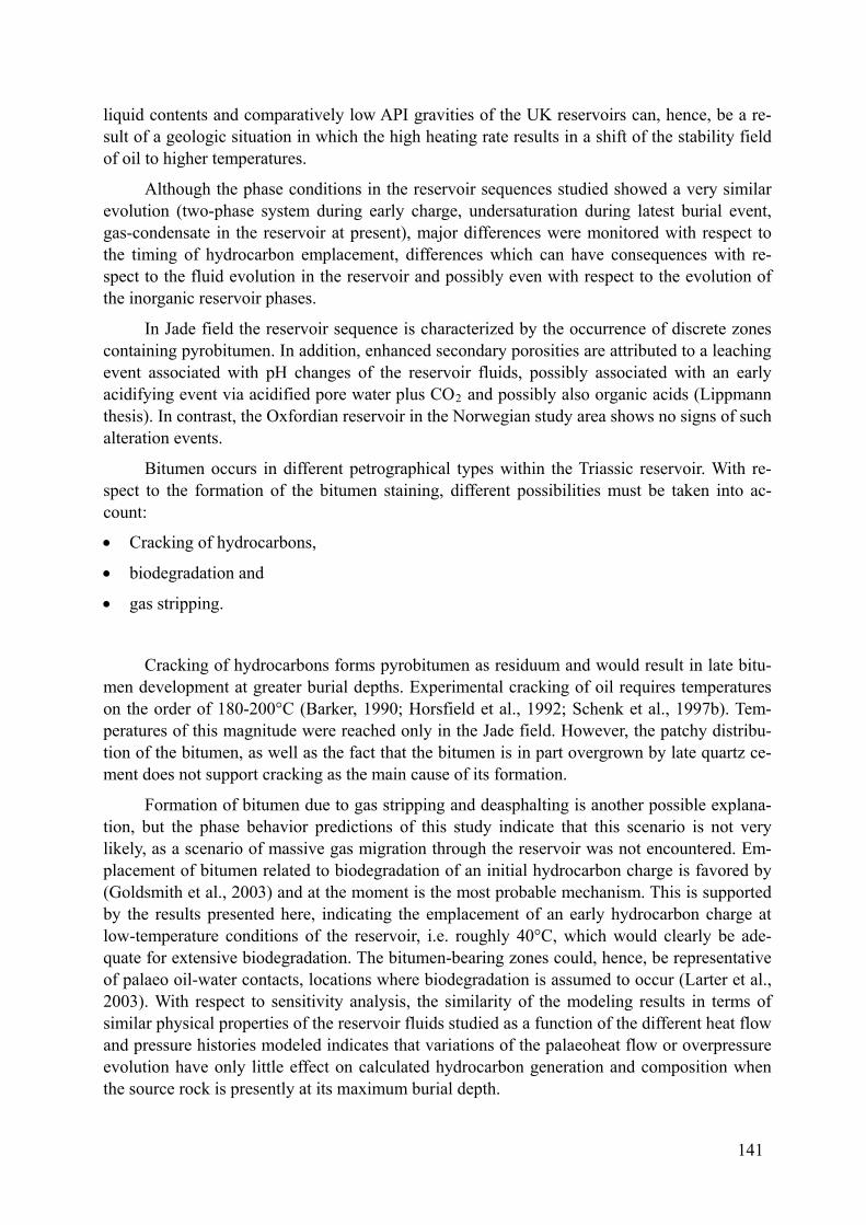
liquid contents and comparatively low API gravities of the UK reservoirs can, hence, be a re-sult of a geologic situation in which the high heating rate results in a shift of the stability field of oil to higher temperatures.

Although the phase conditions in the reservoir sequences studied showed a very similar evolution (two-phase system during early charge, undersaturation during latest burial event, gas-condensate in the reservoir at present), major differences were monitored with respect to the timing of hydrocarbon emplacement, differences which can have consequences with re-spect to the fluid evolution in the reservoir and possibly even with respect to the evolution of the inorganic reservoir phases.

In Jade field the reservoir sequence is characterized by the occurrence of discrete zones containing pyrobitumen. In addition, enhanced secondary porosities are attributed to a leaching event associated with pH changes of the reservoir fluids, possibly associated with an early acidifying event via acidified pore water plus CO2 and possibly also organic acids (Lippmann thesis). In contrast, the Oxfordian reservoir in the Norwegian study area shows no signs of such alteration events.

Bitumen occurs in different petrographical types within the Triassic reservoir. With re-spect to the formation of the bitumen staining, different possibilities must be taken into ac-count:

• Cracking of hydrocarbons,

• biodegradation and

• gas stripping.

Cracking of hydrocarbons forms pyrobitumen as residuum and would result in late bitu-men development at greater burial depths. Experimental cracking of oil requires temperatures on the order of 180-200°C (Barker, 1990; Horsfield et al., 1992; Schenk et al., 1997b). Tem-peratures of this magnitude were reached only in the Jade field. However, the patchy distribu-tion of the bitumen, as well as the fact that the bitumen is in part overgrown by late quartz ce-ment does not support cracking as the main cause of its formation.

Formation of bitumen due to gas stripping and deasphalting is another possible explana-tion, but the phase behavior predictions of this study indicate that this scenario is not very likely, as a scenario of massive gas migration through the reservoir was not encountered. Em-placement of bitumen related to biodegradation of an initial hydrocarbon charge is favored by (Goldsmith et al., 2003) and at the moment is the most probable mechanism. This is supported by the results presented here, indicating the emplacement of an early hydrocarbon charge at low-temperature conditions of the reservoir, i.e. roughly 40°C, which would clearly be ade-quate for extensive biodegradation. The bitumen-bearing zones could, hence, be representative of palaeo oil-water contacts, locations where biodegradation is assumed to occur (Larter et al., 2003). With respect to sensitivity analysis, the similarity of the modeling results in terms of similar physical properties of the reservoir fluids studied as a function of the different heat flow and pressure histories modeled indicates that variations of the palaeoheat flow or overpressure evolution have only little effect on calculated hydrocarbon generation and composition when the source rock is presently at its maximum burial depth.

141

6 Conclusions • 3D basin modeling of the study areas in the Central Graben, North Sea, allowed the charac-

terization of the burial, thermal and hydrocarbon generation and migration histories as well as a description of the reservoir fluid evolution during reservoir filling.

• The integration of bulk kinetics, compositional information from closed system pyrolysis and regional PVT data allowed the definition of a compositional kinetic model which cor-rectly reproduced the observed fluid compositions and physical properties (GOR, saturation pressure and API) using 3D basin modeling.

• The results indicate that in the UK Triassic reservoir early emplacement of petroleum oc-curred. This first hydrocarbon charge consisted of a two phase system (oil and gas) whereby the vapor phase dominated volumetrically. The reservoir conditions upon em-placement were such that biodegradation of this early charge was highly likely. Petro-graphic evidence of extensive, localized bitumen staining supports this assumption.

• Compared to the UK study area, in the Oxfordian reservoir in the Norwegian part of the Central Graben, hydrocarbon emplacement occurred later and at reservoir temperatures above 80°C, thus precluding any significant biotic petroleum alterations.

• The evolution of the fluid phases in the reservoirs in the further burial of the Central Gra-ben evolved along similar lines: reservoir fluids remained in two phases while the GOR in-creased systematically due to source rock maturation and the production of gas-richer pe-troleum compositions.

• Severe overpressures as monitored today in the reservoirs are linked to

• gas generation and

• disequilibrium compaction.

• The rapid development of overpressure in the reservoirs led to the undersaturation of the reservoir fluids, such that today undersaturated gas-condensates are encountered in both fields.

• The present fluid composition is most likely a function of both primary and secondary cracking processes.

Some limitations:

• Digital data quality: This study is nearly exclusively based on pre-generated data, with no control over data-quality. During the loading routine into the modeling software, data inconsistencies, for example crossing horizons, became evident. This may include also other, currently undetected inconsistencies.

• Despite the availability of an extended calibration data set for this study, their quantity is still insufficient with respect to small- and large scale results.

• Uncertainties of petrophysical parameter of the sealing formations like permeability trends are based on literature data and simplified assumptions and have not been re-solved.

• The numerical 3D models were constructed using simplified conceptual models.

143

References

Adamson, K., G. Birch, E. Gao, S. Hand, C. Macdonald, D. Mack and A. Quadri, 1998, High-pressure, high-temperature well construction: Oilfield Review, v. 10, p. 36-49.

Allan, P. A. and J. R. Allen, 1998, Basin Analysis - Principles and Applications: Oxford, Blackwell Sci-ence KK, 451 p.

Andresen, P., N. Mills, H. J. Schenk and B. Horsfield, 1993, The importance of kinetic parameters in modelling generation by cracking oil to gas; a case study in 1D from well 2/ 4-14, Basin model-ling; advances and applications; proceedings of the Norwegian Petroleum Society conference, v. 3: New York, International, Elsevier, p. 563-571.

Aplin, A. C., S. R. Larter, M. A. Bigge, G. Macleod, R. E. Swarbrick and D. Grunberger, 2000, PVTX history of the North Sea's Judy oilfield: Journal of Geochemical Exploration, v. 69-70, p. 641-644.

Athy, L. F., 1930a, Compaction and oil migration: Bulletin of the American Association of Petroleum Geologists, v. 14, p. 25-35.

Athy, L. F., 1930b, Density, porosity, and compaction of sedimentary rocks: Bulletin of the American Association of Petroleum Geologists, v. 14, p. 1-24.

Baldwin, B. and C. O. Butler, 1985, Compaction curves: AAPG Bulletin, v. 69, p. 622-626.

Barker, C., 1972, Aquathermal Pressuring; Role of Temperature in Development of Abnormal-Pressure Zones: The American Association of Petroleum Geologists Bulletin, v. 56, p. 2068-2071.

Barker, C., 1990, Calculated volume and pressure changes during the thermal cracking of oil to gas in reservoirs: AAPG Bulletin (American Association of Petroleum Geologists), v. 74, p. 1254-1261.

Barker, C., A. E. Beck and H. H. Schloessin, 1978, Problems and results of high pressure thermal con-ductivity measurements: Eos, Transactions, American Geophysical Union, v. 59, p. 1029.

Barth, T. and K. Bjorlykke, 1993, Organic acids from source rock maturation; generation potentials, transport mechanisms and relevance for mineral diagenesis: Applied Geochemistry, v. 8, p. 325-337.

Behar, F., S. Kressmann and J. L. Rudkiewicz, 1991, Origin and stability of gaseous compounds gener-ated during thermal cracking of organic matter in sedimentary basins, 201st ACS national meet-ing; abstracts of papers, v. 201; 1: Washington, DC, United States, American Chemical Society, p. GEOC 53.

Behar, F., Y. Tang and J. Liu, 1997a, Comparison of rate constants for some molecular tracers generated during artificial maturation of kerogens: influence of kerogen type: Organic Geochemistry, v. 26, p. 281-287.

Behar, F., M. Vandenbroucke, Y. Tang, F. Marquis and J. Espitalie, 1997b, Thermal cracking of kerogen in open and closed systems; determination of kinetic parameters and stoichiometric coefficients for oil and gas generation: Organic Geochemistry, v. 26, p. 321-339.

145

Berger, G., J.-C. Lacharpagne, B. Velde, D. Beaufort and B. Lanson, 1997, Kinetic constraints on illiti-zation reactions and the effects of organic diagenesis in sandstone/shale sequences: Applied Geochemistry, v. 12, p. 23-35.

Bethke, C. M., 1985, A numerical model of compaction-driven groundwater flow and heat transfer and its application to the paleohydrology of intracratonic sedimentary basins: Jgr, v. Journal of Geophysical Research. B. 90, p. 6817-6828.

Bishop, D. J., 1996, Regional distribution and geometry of salt diapirs and supra-Zechstein Group faults in the western and central North Sea: Marine and Petroleum Geology, v. 13, p. 355-364.

Bjorlykke, K., 1983, Diagenetic reactions in sandstones, in A. Parker, and B. W. Sellwood, eds., Sedi-ment diagenesis. NATO Advanced Study Institute: Co., Reading, UK, Reidel Publ., p. 169-213.

Bjorlykke, K., 1989, Closed versus open system in silicate diagenesis; a review, 28th international geo-logical congress, v. 28; 1: Washington, International Geological Congress, p. 157-158.

Bjorlykke, K., P. Aagaard, P. K. Egeberg and S. P. Simmons, 1995, Geochemical constraints from for-mation water analyses from the North Sea and the Gulf Coast basins on quartz, feldspar and il-lite precipitation in reservoir rocks, The geochemistry of reservoirs, v. 86;: London, United Kingdom, Geological Society of London, p. 33-50.

Bjorlykke, K. and K. Hoeg, 1997, Effects of burial diagenesis on stresses, compaction and fluid flow in sedimentary basins: Marine and Petroleum Geology, v. 14, p. 267-276.

Bolas, H. M. N., C. Hermanrud and G. M. G. Teige, 2004, Origin of overpressures in shales: Constraints from basin modeling: AAPG Bulletin, v. 88, p. 193-211.

Borge, H., 1999, Quantification of mechanisms for generating overpressures in the Haltenbanken re-gion: IAMG conference, p. 509-514.

Borge, H., 2002, Modelling generation and dissipation of overpressure in sedimentary basins: An ex-ample from the Halten Terrace, offshore Norway: Marine and Petroleum Geology, v. 19, p. 377-388.

Bray, E. E. and E. D. Evans, 1961, Distribution of n-paraffins as a clue to recognition of source beds, Symposium on the chemical approaches to the recognition of petroleum source rocks, v. 22; 1: Oxford, International, Pergamon, p. 2-15.

Brooks, J. D., K. Gould and J. W. Smith, 1969, Isoprenoid hydrocarbons in coal and petroleum: Nature (London), v. 222, p. 257-259.

Brosse, E., J. Matthews, B. Bazin, G. Y. Le and F. Sommer, 2000, Related quartz and illite cementation in the Brent sandstones: A modelling approach, in R. H. Worden, and S. Morad, eds., Quartz cementation in sandstones, v. 29: Oxford, International, Blackwell, p. 51-66.

Brown, S., 1991, Stratigraphy of the oil and gas reservoirs - U.K. continental shelf, in I. L. Abbots, ed., United Kingdom oil and gas fields - 25 years commemorative volume, v. 14: London, Geologi-cal Society, p. 9-18.

Bruce, C. H., Altaner, S. P., 1984, Smectite dehydration - its relationship to structural disposition and hydrocarbon migration in the Gulf of Mexico: AAPG Bulletin (American Association of Petro-leum Geologists), v. 68, p. 673-683.

146

Buhrig, C., 1989, Geopressured Jurassic reservoirs in the Viking Graben: Modeling and geological sig-nificance: Marine and Petroleum Geology, v. 6, p. 31-48.

Burley, S. D., 1993, Models of burial diagenesis for deep exploration plays in Jurassic fault traps of the Central and Northern North Sea, in J. R. Parker, ed., Petroleum Geology of Northwest Europe: Proceeding of the 4th Conference, v. 2: London, Geological Society, London, p. 1353-1375.

Byerlee, J., 1993, Model for episodic flow of high-pressure water in fault zones before earthquakes: Geology, v. 21, p. 303-306.

Caillet, G. and S. Batiot, 2003, 2D modelling of hydrocarbon migration along and across growth faults; an example from Nigeria: Petroleum Geoscience, v. 9, p. 113-124.

Carr, A. D., 1999, A vitrinite reflectance kinetic model incorporating overpressure retardation: Marine and Petroleum Geology, v. 16, p. 355-377.

Carr, A. D., 2000, Suppression and retardation of vitrinite reflectance; Part 1, Formation and signifi-cance for hydrocarbon generation: Journal of Petroleum Geology, v. 23, p. 313-343.

Carr, A. D., 2001, Source and timing of diagenesis in North Sea, Upper Jurassic, AAPG Annual Meet-ing (American Association of Petroleum Geologists), Denver, AAPG.

Carr, A. D., 2003, Thermal history model for the South Central Graben, North Sea, derived using both tectonics and maturation: International Journal of Coal Geology, v. 54, p. 3-19.

Cayley, G. T., 1986, Hydrocarbon migration in the central North Sea, in J. Brooks, Glennie, K. W., ed., Petroleum Geology of Northwest Europe: Proceeding of the 3rd Conference, v. 1: London, Geological Society, London, p. 549-556.

Connan, J., 1984, Biodegradation of crude oils in reservoirs, Advances in petroluem geochemistry; Vol-ume 1: London, United Kingdom, Acad Press.

Connan, J., J. Bouroullec, D. Dessort and P. Albrecht, 1986, The microbial input in carbonate-anhydrite facies of a sabkha palaeoenvironment from Guatemala; a molecular approach, Advances in or-ganic geochemistry, 1985; Part I, Petroleum geochemistry, v. 10; 1-3: Oxford-New York, Inter-national, Pergamon, p. 29-50.

Connan, J. and A. M. Cassou, 1980, Properties of gases and petroleum liquids derived from terrestrial kerogen at various maturation levels: Geochimica et Cosmochimica Acta, v. 44, p. 1-24.

Cornford, C., ed., 1994, Mandal-Ekofisk (!) petroleum system in the Central Graben of the North Sea: The petroleum system - from source to trap: AAPG Memoir 60, v. 60: Tulsa, Oklahoma, USA, The American Association of Petroleum Geologists (AAPG), 537-571 p.

Cornford, C., 1998, Source rocks and hydrocarbons of the North Sea, in K. W. Glennie, ed., Petroleum geology of the North Sea: Basic concepts and recent advances: Oxford, United Kingdom, Blackwell Science Geology & Petroleum Geology, p. 376-462.

Dahl, B. and J. H. Augustson, 1993, The influence of Tertiary and Quaternary sedimentation and ero-sion on hydrocarbon generation in Norwegian offshore basins, Basin modelling; advances and applications; proceedings of the Norwegian Petroleum Society conference, v. 3;: New York, In-ternational, Elsevier, p. 419-431.

147

Dahl, J., J. M. Moldowan, K. E. Peters, G. E. Claypool and M. A. Rooney, 1997, Utilization of diamon-doid hydrocarbons for determination of source, thermal maturity and extent of thermal crack-ing, American Association of Petroleum Geologists 1997 annual convention, v. 6;: Tulsa, OK, United States, American Association of Petroleum Geologists and Society of Economic Paleon-tologists and Mineralogists, p. 25.

Dahl, J. E., J. M. Moldowan, K. E. Peters, G. E. Claypool, M. A. Rooney, G. E. Michael, M. R. Mello and M. L. Kohnen, 1999, Diamondoid hydrocarbons as indicators of natural oil cracking: Na-ture, v. 399, p. 54-57.

Darby, D., R. S. Haszeldine and G. D. Couples, 1996, Pressure cells and pressure seals in the UK Cen-tral Graben: Marine and Petroleum Geology, v. 13, p. 865-878.

Darby, D., M. Wilkinson, A. E. Fallick and R. S. Haszeldine, 1997, Illite dates record deep fluid move-ments in petroleum basins: Petroleum Geoscience, v. 3, p. 133-140.

Davison, I., I. Alsop, P. Birch, C. Elders, N. Evans, H. Nicholson, P. Rorison, D. Wade, J. Woodward and M. Young, 2000, Geometry and late-stage structural evolution of Central Graben salt diapirs, North Sea: Marine and Petroleum Geology, v. 17, p. 499-522.

Deegan, C. E. and B. J. Scull, 1977, A proposed standard lithostratigraphic nomenclature for the Meso-zoic of the central and northern North Sea, Mesozoic; northern North Sea symposium 1977 (MNNSS-77); proceedings: Stravanger, Norway, Norwegian Pet Soc.

Deroo, G., B. Durand, J. Espitalie, R. Pelet and B. Tissot, 1969, Possibilite d'application des modeles mathematiques de formation du petrole a la prospection dans les bassins sedimentaires, Ad-vances in organic geochemistry, 1968: Oxford, United Kingdom, Pergamon Press.

di Primio, R., 2000, NH-00010231: Hydro Internal rep.

di Primio, R., 2002, Unraveling secondary migration effects through the regional evaluation of PVT data: a case study from Quadrant 25, NOCS: Organic Geochemistry, v. 33, p. 643-653.

di Primio, R., V. Dieckmann and N. Mills, 1998, PVT and phase behaviour analysis in petroleum explo-ration: Organic Geochemistry, v. 29, p. 207-222.

di Primio, R. and B. Horsfield, 2006, From petroleum type organofacies to hydrocarbon phase predic-tion: AAPG Bulletin, v. 90.

di Primio, R., B. Horsfield and M. A. Guzman-Vega, 2000, Determining the temperature of petroleum formation from the kinetic properties of petroleum asphaltenes: Nature (London), v. 406, p. 173-176.

di Primio, R. and J. E. Skeie, 2004, Development of a compositional kinetic model for hydrocarbon generation and phase equilibria modelling: a case study from Snorre Field, Norwegian North Sea, in J. M. Cubitt, England, W. A., Larter, S., ed., Understanding Petroleum Reservoirs: to-wards an Intefrated Reservoir Engineering and Geochemical Approach, v. 237: London, Geo-logical Society, p. 157-174.

Dickinson, G., 1953, Geological aspects of abnormal reservoir pressures in Guls Coast, Louisiana: AAPG Bulletin (American Association of Petroleum Geologists), v. 37, p. 410-432.

Didyk, B. M., B. R. T. Simoneit, S. C. Brassell and G. Eglinton, 1978, Organic geochemical indicators of palaeoenvironmental conditions of sedimentation: Nature (London), v. 272, p. 216-222.

148

Dieckmann, V., 2005, Modelling petroleum formation from heterogeneous source rocks: the influence of frequency factors on activation energy distribution and geological prediction: Marine and Pe-troleum Geology, v. 22, p. 375-390.

Dieckmann, V., H. J. Schenk, B. Horsfield and D. H. Welte, 1998, Kinetics of petroleum generation and cracking by programmed-temperature closed-system pyrolysis of Toarcian Shales: Fuel, v. 77, p. 23-31.

Donovan, A. D., Djakic, A. W., Ioannides, N. S., Garfield, G. R., Jones, C. R., 1993, Sequence strati-graphic control on Middle and Upper Jurassic reservoir distribution within the UK Central North Sea, in J. R. Parker, ed., Petroleum geology of northwest Europe: Proceeding of the 4th conference, v. 1: London, Geological Society, p. 251-269.

Dueppenbecker, S. and B. Horsfield, 1990, Compositional information for kinetic modelling and petro-leum type prediction, Advances in organic geochemistry 1989; Part I, Organic geochemistry in petroleum exploration, v. 16; 1-3: Oxford-New York, International, Pergamon, p. 259-266.

Durand, B., P. Ungerer, A. Chiarelli and J. L. Oudin, 1984, Modelisation de la migration de l'huile; ap-plication adeux exemples de bassins sedimentaires: Proceedings - World Petroleum Congress = Actes et Documents - Congres Mondial du Petrole, v. 11, p. 3-15.

EERTAG, 1997, An assessment of the evacuation of an offshore installation by TEMPSC - based on an analysis of survivor experiences, p. 36.

England, W. A., 1990, The organic geochemistry of petroleum reservoirs, Advances in organic geo-chemistry 1989; Part I, Organic geochemistry in petroleum exploration, v. 16; 1-3: Oxford-New York, International, Pergamon, p. 415-425.

England, W. A. and A. S. Mackenzie, 1989, Some aspects of the organic geochemistry of petroleum flu-ids: Geologische Rundschau, v. 78, p. 291-303.

England, W. A., A. S. Mackenzie, D. M. Mann and T. M. Quigley, 1987, The movement and entrapment of petroleum fluids in the subsurface, Two-phase flow in crust and mantle, v. 144; 2: London, United Kingdom, Geological Society of London, p. 327-347.

Erdmann, M., 1999, Gas generation from overmature Upper Jurassic source rocks, northern Viking Graben: Doctoral thesis, RWTH, Aachen. Berichte des Forschungszentrums Jülich; 3700, 128 p.

Erratt, D., G. M. Thomas and G. R. T. Wall, 1999, The evolution of the central North Sea Rift, Petro-leum geology of Northwest Europe; proceedings of the 5th conference, v. Conference. 5;: Lon-don, United Kingdom, The Geological Society of London, p. 63-82.

Espitalie, J., F. Marquis and S. Drouet, 1993, Critical study of kinetic modelling parameters, Basin modelling: Advances and applications; proceedings of the Norwegian Petroleum Society con-ference, v. 3: New York, International, Elsevier, p. 233-242.

Espitalie, J., P. Ungerer, I. Irwin and F. Marquis, 1988, Primary cracking of kerogens; experimenting and modeling C , C -C , C -C and C1 2 5 6 15 15+ classes of hydrocarbons formed, Advances in or-ganic geochemistry 1987; Part II, Analytical geochemistry; proceedings of the 13th interna-tional meeting on Organic geochemistry, v. 13; 4-6: Oxford-New York, International, Perga-mon, p. 893-899.

149

Evans, D., C. Graham, A. Armour and P. Bathurst, 2003, The millennium atlas; petroleum geology of the central and northern North Sea: London, United Kingdom, Geological Society of London, 389 p.

Fein, J. B., 1991a, Experimental study of aluminum-, calcium-, and magnesium-acetate complexing at 80 degrees C: Geochimica et Cosmochimica Acta, v. 55, p. 955-964.

Fein, J. B., 1991b, Experimental study of aluminum-oxalate complexing at 80°C; implications for the formation of secondary porosity within sedimentary reservoirs: Geology (Boulder), v. 19, p. 1037-1040.

Fisher, M. J. and D. C. Mudge, 1998, Triassic, in K. W. Glennie, ed., Petroleum geology of the North Sea: Basic concepts and recent advances: Oxford, United Kingdom, Blackwell Science Geol-ogy & Petroleum Geology.

Fraser, S., A. Robinson, H. Johnson, J. Underhill, D. Kadolsky, R. Connell, P. Johannessen and R. Rav-nas, 2003, Upper Jurassic, The millennium atlas; petroleum geology of the central and northern North Sea: London, United Kingdom, Geological Society of London.

Frederiksen, S., S. B. Nielsen and N. Balling, 2001, A numerical dynamic model for the Norwegian-Danish Basin: Tectonophysics, v. 343, p. 165-183.

Fritz, S. J., Marine, W., 1983, Experimental support for a predictive model of clay membranes: Geo-chimica et Cosmochimica Acta, v. 47, p. 1515-1522.

Gaarenstroom, L., R. A. J. Tromp, M. C. de Jong and A. M. Brandenburg, 1993, Overpressures in the central North Sea; implications for trap integrity and drilling safety, Petroleum geology of Northwest Europe; Proceedings of the 4th conference, v. Conference 4: London, United King-dom, The Geological Society of London, p. 1305-1313.

Gabrielsen, R. H., R. Kyrkjebo, J. I. Faleide, W. Fjeldskaar and T. Kjennerud, 2001, The Cretaceous post-rift basin configuration of the northern North Sea: Petroleum Geoscience, v. 7, p. 137-154.

Gaupp, R., A. Matter, J. Platt, K. Ramseyer and J. Walzebuck, 1993, Diagenesis and fluid evolution of deeply buried Permian (Rotliegende) gas reservoirs, Northwest Germany: AAPG Bulletin (American Association of Petroleum Geologists), v. 77, p. 1111-1128.

Giles, M. R., R. B. de Boer and J. D. Marshall, 1994, How important are organic acids in generating secondary porosity in the subsurface?, in E. D. Pittman, and M. D. Lewan, eds., Organic Acids in Geological Processes: New York, NY, United States, Springer-Verlag, p. 447-468.

Giles, M. R., S. L. Indrelid and D. M. D. James, 1998, Compaction; the great unknown in basin model-ling, Basin modelling; practice and progress, v. 141;: London, United Kingdom, Geological So-ciety of London, p. 15-43.

Glennie, K. W., 1998a, Lower Permian, Rotliegend, in K. W. Glennie, ed., Petroleum geology of the North Sea: Basic concepts and recent advances: Oxford, United Kingdom, Blackwell Science Geology & Petroleum Geology.

Glennie, K. W., 1998b, Lower Permian-Rotliegend, in K. W. Glennie, ed., Petroleum geology of the North Sea: Oxford, Blackwell Science Ltd., p. 137-173.

Glennie, K. W., 1998c, Origin, development and evolution of structural styles, in K. W. Glennie, ed., Petroleum geology of the North Sea: Oxford, Blackwell Science Ltd., p. 42-84.

150

Glennie, K. W. and J. R. Underhill, 1998, Origin, development and evolution of structural styles, in K. W. Glennie, ed., Petroleum geology of the North Sea: Basic concepts and recent advances: Ox-ford, United Kingdom, Blackwell Science Geology & Petroleum Geology.

Glover, P. W., 1999, Formation evaluation: Aberdeen, UK, Department of geology and petroleum geol-ogy.

Gluyas, J. and A. Leonard, 1995, Diagenesis of the Rotliegend Sandstone: The answer ain't blowin' in the wind: Marine and Petroleum Geology, v. 12, p. 491-497.

Gluyas, J. G., 1997, Poroperm prediction for reserves growth exploration; Ula Trend, Norwegian North Sea, Reservoir quality prediction in sandstones and carbonates, v. 69: Tulsa, OK, United States, American Association of Petroleum Geologists, p. 201-210.

Gluyas, J. G. and C. A. Cade, 1997, Prediction of porosity in compacted sands, Reservoir quality predic-tion in sandstones and carbonates, v. 69: Tulsa, OK, United States, American Association of Pe-troleum Geologists, p. 19-27.

Goldsmith, P. J., G. Hudson, V. P. van, P. Slater, K. S. Lervik, M. Bergan, G. W. Diesen, C. Stockbridge, H. Kerr, G. D. Harris, J. P. Gibson, R. Bayes, T. Keller, R. Blakey and B. Trudgill, 2003, Trias-sic, The millennium atlas; petroleum geology of the central and northern North Sea: London, United Kingdom, Geological Society of London.

Hantschel, T., A. I. Kauerauf and B. Wygrala, 2000, Finite element analysis and ray tracing modeling of petroleum migration: Marine and Petroleum Geology, v. 17, p. 815-820.

Harrison, W. J. and G. D. Thyne, 1994, Geochemical models of rock-water interactions in the presence of organic acids, Organic acids in geological processes: New York, NY, United States, Springer-Verlag.

Haszeldine, R. S. e. a., 1999, Diagenetic porosity creation in an overpressured graben, in A. J. B. Fleet, S. A. R., ed., Petroleum Geology of Northwest Europe: Proceeding of the 5th Conference, v. 2: London, Geological Society, p. 1339-1350.

Hendry, J. P., M. Wilkinson, A. E. Fallick and R. S. Haszeldine, 2000, Ankerite cementation in deeply buried Jurassic sandstone reservoirs of the central North Sea: Journal of Sedimentary Research, v. 70, p. 227-239.

Hermanrud, C., 1993, Basin modelling techniques; an overview, Basin modelling; advances and appli-cations; proceedings of the Norwegian Petroleum Society conference, v. 3;: New York, Interna-tional, Elsevier, p. 1-34.

Hermanrud, C., S. Eggen, T. Jacobsen, E. M. Carlsen and S. Pallesen, 1990, On the accuracy of model-ling hydrocarbon generation and migration; the Egersund Basin oil find, Norway, Advances in organic geochemistry 1989; Part I, Organic geochemistry in petroleum exploration, v. 16; 1-3: Oxford-New York, International, Pergamon, p. 389-399.

Hodgson, N. A., J. Farnsworth and A. J. Fraser, 1992, Salt-related tectonics, sedimentation and hydro-carbon plays in the Central Graben, North Sea, UKCS: Exploration Britain: geological insights for the next decade, Published by Geological Society, London; Special Publication, 67, Editors Hardman R.F.P., p. 31-63.

151

Holm, G. M., ed., 1998, Distribution and origin of overpressure in the Central Graben of the North Sea: Abnormal pressures in hydrocarbon environments: AAPG Memoir 70, v. 70: Tulsa, Oklahoma, USA, The American Association of Petroleum Geologists (AAPG), 123-144 p.

Horsfield, B., 1989, Practical criteria for classifying kerogens: Some observations from pyrolysis-gas chromatography: Geochimica et Cosmochimica Acta, v. 53, p. 891-901.

Horsfield, B., H. J. Schenk, N. Mills and D. H. Welte, 1992, An investigation of the in-reservoir conver-sion of oil to gas; compositional and kinetic findings from closed-system programmed-temperature pyrolysis, Advances in organic geochemistry 1991; Part 1, Advances and applica-tions in energy and the natural environment, v. 19; 1-3: Oxford-New York, International, Per-gamon, p. 191-204.

Hughes, W. B., A. G. Holba, D. E. Miller and J. S. Richardson, 1985, Geochemistry of greater Ekofisk crude oils, Petroleum geochemistry in exploration of the Norwegian Shelf: London, United Kingdom, Graham and Trotman.

IES, 2002, PetroMod© Reference Manual - version 8.0, Jülich, Germany, Jülich, Germany.

Isaksen, G., 2004, Central North Sea hydrocarbon systems: Generation, migration, entrapment, and thermal degradation of oil and gas: AAPG Bulletin, v. 88, p. 1545-1572.

Jackson, M. P., Talbot, C. J., 1986, External shapes, strain rates, and dynamics of salt structures: AAPG Bulletin (American Association of Petroleum Geologists), v. 97, p. 305-323.

Jarvie, D. M., 1991, Factors affecting Rock-Eval derived kinetic parameters, Organic geochemistry of hydrocarbon basins, v. 93; 1-2: Amsterdam, Netherlands, Elsevier, p. 79-99.

Jensen, R. P. and A. G. Doré, 1993, A recent Norwegian Shelf heating event - fact or fantasy?, Basin modelling; advances and applications; proceedings of the Norwegian Petroleum Society con-ference, v. 3: New York, International, Elsevier, p. 85-106.

Jensen, T. F. and B. Buchardt, 1987, Sedimentology and geochemistry of the organic carbon-rich Lower Cretaceous Sola Formation (Barremian-Albian), Danish North Sea, Petroleum geology of North West Europe: London, United Kingdom, Graham & Trotman.

Johansen, H., K. Iden, G. Aberg and K. Aasgaard, 1997, Importance of coal layers for reservoir diagene-sis and reservoir compartmentalization, 59th EAGE conference and technical exhibition; ex-tended abstracts; Volume 2, Oral and poster presentations; Petroleum Division, v. 59;, p.; abstr.

Johnson, H. D. and M. J. Fisher, 1998, North Sea plays; geological controls on hydrocarbon distribu-tion, in K. W. Glennie, ed., Petroleum geology of the North Sea: Basic concepts and recent ad-vances: Oxford, United Kingdom, Blackwell Science Geology & Petroleum Geology, p. 463-548.

Jones, A. D., Auld, H. A., Carpenter, T. J., Fetkovich, E., Palmer, I. A., Rigatos, E. N., and Thompson, M. W., 2004, Jade Field: An innovative approach to high-pressure/high-temperature field de-velopment, in A. G. Doré, Vining, B., ed., Petroleum Geology: North-West Europe and Global Perspectives-Proceedings of the 6th Petroleum Geology Conference, The Geological Society, p. 1-16.

Jones, R. W., 1987, Organic facies, Advances in petroleum geochemistry, v. 2: London-Orlando-Toronto, United Kingdom, Academic Press, p. 1-90.

152

Khavari, K. G., J. C. Dolson and J. K. Michelsen, 1998a, The factors controlling the abundance and mi-gration of heavy versus light oils, as constrained by data from the Gulf of Suez; Part I, The ef-fect of expelled petroleum composition, PVT properties and petroleum system geometry, Ad-vances in organic geochemistry 1997; proceedings of the 18th international meeting on Organic geochemistry; Part 1, Petroleum geochemistry, v. 29; 1-3: Oxford-New York, International, Pergamon, p. 255-282.

Khavari, K. G., J. K. Michelsen and J. C. Dolson, 1998b, The factors controlling the abundance and mi-gration of heavy vs. light oils, as constrained by data from the Gulf of Suez; Part II, The signifi-cance of reservoir mass transport processes, Advances in organic geochemistry 1997; proceed-ings of the 18th international meeting on Organic geochemistry; Part 1, Petroleum geochemis-try, v. 29; 1-3: Oxford-New York, International, Pergamon, p. 283-300.

Killops, S. D. and V. J. Killops, 1993, An Introduction to Organic Geochemistry: New York, Blackwell Publishing, 393 p.

Kubala, M., M. Bastow, S. Thompson, I. Scotchman and K. Oygard, 2003, Geothermal regime, petro-leum generation and migration, in D. Evans, Graham, C, Armour, A, and Bathurst, P, ed., The millennium atlas; petroleum geology of the central and northern North Sea: London, United Kingdom, Geological Society of London, p. 289-315.

Kuo, L. C. and G. E. Michael, 1994, A multicomponent oil-cracking kinetics model for modeling pres-ervation and composition of reservoired oils: Organic Geochemistry, v. 21, p. 911-925.

Kvenvolden, K. A. and B. R. T. Simoneit, 1990, Hydrothermally derived petroleum; examples from Guaymas Basin, Gulf of California, and Escanaba Trough, Northeast Pacific Ocean: AAPG Bulletin, v. 74, p. 223-237.

Landa, S. and V. Machacek, 1933, Adamantane, a new hydrocarbon extracted from petroleum: Collec-tion of Czechoslovak Chemical Communications, v. 5, p. 1-5.

Larter, S., A. Wilhelms, I. Head, M. Koopmans, A. Aplin, R. Di Primio, C. Zwach, M. Erdmann and N. Telnaes, 2003, The controls on the composition of biodegraded oils in the deep subsurface - part 1: Biodegradation rates in petroleum reservoirs: Organic Geochemistry, v. 34, p. 601-613.

Law, B. E., Spencer, C. W., ed., 1998, Abnormal pressures in hydrocarbon environments: Abnormal pressures in hydrocarbon environments: AAPG Memoir 70, v. 70: Tulsa, Oklahoma, USA, The American Association of Petroleum Geologists, 1-11 p.

Lee, Y. and D. Deming, 2002, Overpressures in the Anadarko Basin, southwestern Oklahoma; static or dynamic?: AAPG Bulletin, v. 86, p. 145-160.

Leonard, R. C., 1993, Distribution of sub-surface pressure in the Norwegian Central Graben and appli-cations for exploration, in J. R. Parker, ed., Petroleum Geology of Northwest Europe: Proceed-ing of the 4th Conference, v. 2: London, Geological Society, London, p. 1295-1303.

Lerche, I. and W. H. Glezen, 1984, Deposition, compaction and fluid migration: Time-depended models in one and two dimensions, Gulf research and development: Pittsburgh, p. 52.

Lerche, I., R. F. Yarzab and C. G. S. C. Kendall, 1984, Determination of paleoheat flux from vitrinite re-flectance data: AAPG Bulletin, v. 68, p. 1704-1717.

LGC-Geochemistry, 1997, Confidental Report.

153

Luo, X., Vasseur, G., 1992, Contributions of compaction and aquathermal pressuring to geopressure and the influence of environmental conditions: AAPG Bulletin (American Association of Petroleum Geologists), v. 76, p. 1550-1559.

Magoon, L. B. and W. G. Dow, 1994, The petroleum system, The petroleum system; from source to trap, v. 60;: Tulsa, OK, United States, American Association of Petroleum Geologists, p. 3-24.

Mallon, A. J. and R. E. Swarbrick, 2002, A compaction trend for non-reservoir North Sea Chalk: Ma-rine and Petroleum Geology, v. 19, p. 527-539.

Mango, F. D., 1997, The light hydrocarbons in petroleum: a critical review: Organic Geochemistry, v. 26, p. 417-440.

Mango, F. D., 2001, Methane concentrations in natural gas: the genetic implications: Organic Geo-chemistry, v. 32, p. 1283-1287.

Matthes, S., 1993, Mineralogie: Berlin Heidelberg New York, Springer-Verlag, 461 p.

McKenzie, D., 1978, Some remarks on the development of sedimentary basins: Earth and Planetary Science Letters, v. 40, p. 25-32.

Meulbroek, P., 2002, Equations of state in exploration: Organic Geochemistry, v. 33, p. 613-634.

Meulbroek, P. and G. MacLeod, 2002, PVT properties in exploration: Organic Geochemistry, v. 33, p. 611-612.

Monnett, V. E., 1922, Possible origin of some of the structures of the Mid-Continent oil field: Economic Geology and the Bulletin of the Society of Economic Geologists, v. 17, p. 194-200.

Mosar, J., G. Lewis and T. H. Torsvik, 2002, North Atlantic sea-floor spreading rates; implications for the Tertiary development of inversion structures of the Norwegian-Greenland Sea: Journal of the Geological Society of London.

Moss, B., Barson, D, Rakhit, K, Dennis, H, and Swarbrick, R., 2003, Formation pore pressures and formation waters, in D. Evans, Graham, C, Armour, A, and Bathurst, P, ed., The Millennium At-las: petroleum geology of the central and northern North Sea.: London, The Geological Society of London, p. 317-329.

Nelson, L. and E. Obert, 1954, How to use the new generalized compressibility charts: Chemical Engi-neering, v. 61, p. 203-208.

Nielsen, S. B., 1996, Sensitivity analysis in thermal and maturity modelling: Marine and Petroleum Ge-ology, v. 13, p. 415-425.

Oakman, C. D. and M. A. Partington, 1998, Cretaceous, in K. W. Glennie, ed., Petroleum geology of the North Sea: Basic concepts and recent advances: Oxford, United Kingdom, Blackwell Science Geology & Petroleum Geology, p. 294-349.

Osborne, M. J. and R. E. Swarbrick, 1997, Mechanisms of generating overpressure in sedimentary ba-sins: A reevaluation: AAPG Bulletin (American Association of Petroleum Geologists), v. 81, p. 1023-1041.

Osborne, M. J. and R. E. Swarbrick, 1999, Diagenesis in North Sea HPHT clastic reservoirs - conse-quences for porosity and overpressure prediction: Marine and Petroleum Geology, v. 16, p. 337-353.

154

Parkes, R. J., B. A. Cragg, S. J. Bale, J. M. Getliff, K. Goodman, P. A. Rochelle, J. C. Fry, A. J. Weightman and S. M. Harvey, 1994, Deep bacterial biosphere in Pacific Ocean sediments: Na-ture (London), v. 371, p. 410-413.

Patel, V., E. Decoster, A. Douglas, R. Chambers, O. Mullins, X. Wu, M. Kane, P. Rabbito, T. Terabaya-shi, N. Itagaki and J. Singer, 1997, Evaluation of new wells: Venezuela well evaluation confer-ence, p. 1-14.

Pepper, A. S. and P. J. Corvi, 1995a, Simple kinetic models of petroleum formation. Part I: Oil and gas generation from kerogen: Marine and Petroleum Geology, v. 12, p. 291-319.

Pepper, A. S. and P. J. Corvi, 1995b, Simple kinetic models of petroleum formation. Part III: Modelling an open system: Marine and Petroleum Geology, v. 12, p. 417-452.

Peress, J., 2003, Working with non-ideal gases: Chemical Engineering Progress (CEP), v. 99, p. 39-41.

Poelchau, H. S., D. R. Baker, T. Hantschel, B. Horsfield and B. Wygrala, 1997, Basin simulation and the design of the conceptual basin model, in D. H. Welte, B. Horsfield, and D. R. Baker, eds., Petroleum and basin evolution; insights from petroleum geochemistry, geology and basin mod-eling: Berlin, Federal Republic of Germany, Springer, p. 3-70.

Powell, T. G., H. H. L. ten, J. Rullkoetter, L. J. W. de and D. J. S. Sinninghe, 1988, Pristane/ phytane ra-tio as environmental indicator; discussion and reply: Nature (London), v. 333, p. 604.

Quigley, T. M., A. S. Mackenzie and J. R. Gray, 1987, Kinetic theory of petroleum generation, Migra-tion of hydrocarbons in sedimentary basins, v. 45: Paris, France, Technip, p. 649-665.

Radke, M., B. Horsfield, R. Littke and J. Rullkoetter, 1997, Maturation and petroleum generation, in D. H. Welte, B. Horsfield, and D. R. Baker, eds., Petroleum and basin evolution; insights from pe-troleum geochemistry, geology and basin modeling: Berlin, Federal Republic of Germany, Springer, p. 169-229.

Rattey, R. P. and A. P. Hayward, 1993, Sequence stratigraphy of a failed rift system: The Middle Juras-sic to Early Cretaceous basin evolution of the Central and Northern North Sea, in J. R. Parker, ed., Petroleum Geology of Northwest Europe: Proceeding of the 4th Conference, v. 1: London, Geological Society, London, p. 215-249.

Rubey, W. W. and M. K. Hubbert, 1959, Overthrust belt in geosynclinal area of western Wyoming in light of fluid-pressure hypothesis, [Part] 2 of Role of fluid pressure in mechanics of overthrust faulting: Geological Society of America Bulletin, v. 70, p. 167-205.

Rullkotter, J., P. K. Mukhopadhyay, R. G. Schaefer and D. H. Welte, 1984, Geochemistry and petrogra-phy of organic matter in sediments from Deep Sea Drilling Project sites 545 and 547, Mazagan Escarpment, Initial reports of the Deep Sea Drilling Project; Las Palmas, Grand Canary Island to Brest, France, July-December, 1979, v. 79;: College Station, TX, United States, Texas A & M University Ocean Drilling Program, p. 775-805.

Schatzinger, R. A., Feazel, C. T., Henry, W. E., 1985, Evidence of resedimentation in Chalk from the Central Graben, North Sea., in P. D. Crevello, Harris, P. M., ed., SEPM Core workshop No. 6: New Orleans, Society of Economic Palaeonological Mineralogists, p. 342-389.

155

Schenk, H. J., R. Di Primio and B. Horsfield, 1997a, The conversion of oil into gas in petroleum reser-voirs. Part 1: comparative kinetic investigation of gas generation from crude oils of lacustrine, marine and fluviodeltaic origin by programmed-temperature closed-system pyrolysis: Organic Geochemistry, v. 26, p. 467-481.

Schenk, H. J. and B. Horsfield, 1998, Using natural maturation series to evaluate the utility of parallel reaction kinetics models; an investigation of Toarcian shales and Carboniferous coals, Ger-many, Advances in organic geochemistry 1997; proceedings of the 18th international meeting on Organic geochemistry; Part 1, Petroleum geochemistry, v. 29; 1-3: Oxford-New York, Inter-national, Pergamon, p. 137-154.

Schenk, H. J., B. Horsfield, B. Krooss, R. G. Schaefer and K. Schwochau, 1997b, Kinetics of petroleum formation and cracking, Petroleum and basin evolution; insights from petroleum geochemistry, geology and basin modeling: Berlin, Federal Republic of Germany, Springer.

Schlumberger, 2005, Oilfield Glossary, Schlumberger.

Schneider, F., J. L. Potdevin and I. Faille, 1994, New compaction model for the simulation of sedimen-tary basins, AAPG annual convention, v. 1994;: Tulsa, OK, United States, American Associa-tion of Petroleum Geologists and Society of Economic Paleontologists and Mineralogists, p. 252.

Schneider, F. and S. Wolf, 2000, Quantitative HC potential evaluation using 3D basin modelling: appli-cation to Franklin structure, Central Graben, North Sea, UK: Marine and Petroleum Geology, v. 17, p. 841-856.

Scholle, P. A., 1977, Chalk Diagenesis and its relation to petroleum exploration: Oil from chalks - a modern miracle?: AAPG Bulletin, v. 61, p. 982-1009.

Sclater, J. G. and P. A. F. Christie, 1980a, Continental stretching: an explanation of the post-mid-Cretaceous subsidence of the central North Sea basin: Journal of Geophysical Research, v. 85, p. 3711-3739.

Sclater, J. G. and P. A. F. Christie, 1980b, Continental stretching; an explanation of the post-Mid-Cretaceous subsidence of the central North Sea basin: Journal of Geophysical Research, v. 85, p. 3711-3739.

Scotchman, I. C., C. E. Griffith, A. J. Holmes and D. M. Jones, 1998, The Jurassic petroleum system north and west of Britain: a geochemical oil-source correlation study: Organic Geochemistry, v. 29, p. 671-700.

Seifert, W. K. and J. M. Moldowan, 1980, The effect of thermal stress on source-rock quality as meas-ured by hopane stereochemistry, Advances in organic geochemistry 1979, v. 12;: Oxford-New York-Toronto, International, Pergamon, p. 229-237.

Sheriff, R. E., 1990, Encyclopedic dictionary of exploration geophysics. 3 ed: Explor. Geophys.. Tulsa, OK, United States, Soc, 376 p.

Slavin, V. I., Smirnova, E. M., 1998, Abnormally high formation pressures: Origin, prediction, hydro-carbon field development, and ecological problems, in B. E. Law, Ulmishek, G.F., Slavin, V. I., ed., Abnormal pressures in hydrocarbon environments: AAPG Memoir 70, v. 70: Tulsa, Okla-homa, USA, The American Association of Petroleum Geologists, p. 105-114.

156

Sørensen, K., 1986, Danish basin subsidence by Triassic rifting on a lithosphere cooling background: Nature, v. 319, p. 660-663.

Surdam, R. C., S. W. Boese and L. J. Crossey, 1984, The chemistry of secondary porosity, Clastic diagenesis, v. 37;: Tulsa, OK, United States, American Association of Petroleum Geologists, p. 127-149.

Surdam, R. C. and L. J. Crossey, 1985, Organic-inorganic reactions during progressive burial; key to porosity and permeability enhancement and preservation, Geochemistry of buried sediments, v. 315; 1531: London, United Kingdom, Royal Society of London, p. 135-156.

Swarbrick, R. E., M. J. Osborne, D. Grunberger, G. S. Yardley, G. Macleod, A. C. Aplin, S. R. Larter, I. Knight and H. A. Auld, 2000, Integrated study of the Judy Field (Block 30/7a) - an overpres-sured Central North Sea oil/gas field: Marine and Petroleum Geology, v. 17, p. 993-1010.

Swarbrick, R. E., Osborne, M. J., 1998, Mechanisms that generate abnormal pressures: An overview, in B. E. Law, Ulmishek, G.F., Slavin, V. I., ed., Abnormal pressures in hydrocarbon environments: AAPG Memoir 70, v. 70: Tulsa, Oklahoma, USA, The American Association of Petroleum Ge-ologists, p. 13-34.

Sweeney, J. and A. K. Burnham, 1990, Evaluation of a simple model of vitrinite reflectance based on chemical kinetics: AAPG Bulletin, v. 74, p. 1559-1570.

Taylor, J. C. M., 1997, Upper Permian-Zechstein, in K. W. Glennie, ed., Petroleum geology of the North Sea: Oxford, Blackwell Science Ltd., p. 174-210.

Taylor, J. C. M., 1998, Upper Permian, Zechstein, in K. W. Glennie, ed., Petroleum geology of the North Sea: Basic concepts and recent advances: Oxford, United Kingdom, Blackwell Science Geology & Petroleum Geology, p. 174-210.

Teige, G. M. G., C. Hermanrud, L. Wensaas and H. M. N. Bolas, 1999, The lack of relationship between overpressure and porosity in North Sea and Haltenbanken shales: Marine and Petroleum Geol-ogy, v. 16, p. 321-335.

ten Haven, H. L., J. W. de Leeuw, J. Rullkoetter and D. J. S. Sinninghe, 1987, Restricted utility of the pristane/ phytane ratio as a palaeoenvironmental indicator: Nature (London), v. 330, p. 641-643.

Thyne, G., B. P. Boudreau, M. Ramm and R. E. Midtbo, 2001, Simulation of potassium feldspar disso-lution and illitization in the Statfjord Formation, North Sea: AAPG Bulletin (American Asso-ciation of Petroleum Geologists), v. 85, p. 621-635.

Tissot, B., 1969, Premieres donnees sur les mecanismes et la cinetique de la formation du petrole dans les sediments; simulation d'un schema reactionnel sur ordinateur: Revue de l'Institut Francais du Petrole, v. 24, p. 470-501.

Tissot, B. and J. Espitalie, 1975, L'evolution thermique de la matiere organique des sediments; applica-tions d'une simulation mathematique; Potentiel petrolier des bassins sedimentaires et reconstitu-tion de l'histoire thermique des sediments: Revue de l'Institut Francais du Petrole et Annales des Combustibles Liquides, v. 30, p. 743-777.

Tissot, B. P., R. Pelet and P. Ungerer, 1987, Thermal history of sedimentary basins, maturation indices, and kinetics of oil and gas generation: AAPG Bulletin, v. 71, p. 1445-1466.

157

Tissot, B. P. and D. H. Welte, 1984, Petroleum formation and occurrence. 2 ed: Berlin, Federal Republic of Germany, Springer-Verlag, 699 p.

Torre, M. D., R. F. Mahlmann and W. G. Ernst, 1997, Experimental study on the pressure dependence of vitrinite maturation: Geochimica et Cosmochimica Acta, v. 61, p. 2921-2928.

Turner, P., M. Jones, D. J. Prosser, G. D. Williams and A. Searl, 1993, Structural and sedimentological controls on diagenesis in the Ravenspurn North gas reservoir, UK southern North Sea, Petro-leum geology of Northwest Europe; Proceedings of the 4th conference, v. Conference. 4: Lon-don, United Kingdom, The Geological Society of London, p. 771-785.

Tyson, R. V., Funnel, B.M., 1987, European Cretaceous shorelines, stage by stage, in E. J. Barron, ed., Cretaceous Paleogeography, v. 59, Special Publication of the Palaeogeography, Palaeoclima-tololgy and Palaeoecology, p. 69-91.

Underhill, J. R., 1998a, Jurassic, in K. W. Glennie, ed., Petroleum geology of the North Sea: Oxford, Blackwell Science Ltd., p. 245-293.

Underhill, J. R., 1998b, Jurassic, in K. W. Glennie, ed., Petroleum geology of the North Sea: Basic con-cepts and recent advances: Oxford, United Kingdom, Blackwell Science Geology & Petroleum Geology, p. 245-293.

Underhill, J. R., 2003, The tectonic and stratigraphic framework of the United Kingdom's oil and gas fields, United Kingdom oil and gas fields commemorative millennium volume, v. 20;: Bath, United Kingdom, Geological Society Publishing House, p. 17-59.

Ungerer, P., 1990, State of the art of research in kinetic modelling of oil formation and expulsion, Ad-vances in organic geochemistry 1989; Part I, Organic geochemistry in petroleum exploration, v. 16; 1-3: Oxford-New York, International, Pergamon, p. 1-25.

Ungerer, P., Bessis, F., Chenet, P. Y., ed., 1984, Geological and geochemical models of oil exploration; principles and practical examples: Petroleum geochemistry and basin evolution, v. AAPG Memoir 35: Tulsa, Oklahoma, USA, The American Association of Petroleum Geologists (AAPG).

Vail, P. R., Todd, R. G., 1981, Northern North Sea Jurassic unconformities, chronostratigraphy and sea level changes from seismic stratigraphy, in L. V. Illings, Hobson, G. D., ed., Petroleum geology of the continental shelf of northwest Europe: London, Institute of Petroleum, p. 216-235.

Vandenbroucke, M., F. Behar and J. L. Rudkiewicz, 1999, Kinetic modelling of petroleum formation and cracking: implications from the high pressure/high temperature Elgin Field (UK, North Sea)*1: Organic Geochemistry, v. 30, p. 1105-1125.

Vollset, J. and A. G. Doré, 1984, A revised Triassic and Jurassic lithostratigraphic nomenclature for the Norwegian North Sea.: Bulletin of the Norwegian Petroleum Directorate, v. 3.

Waples, D. and T. Machihara, 1991, Biomarkers for Geologists - A Practical Guide to the Application of Sternanes and Triterpanes in Petroleum Geology: AAPG Methods in Exploration, v. 9.

Waples, D. W., 1983, Physical-chemical models for oil generation, Research in chemistry and geochem-istry at Colorado School of Mines; a tribute to L J Beckham; Part 2, v. 78; 4: Golden, CO, United States, Colorado School of Mines, p. 15-30.

158

Ward, C. D., Coghill, K., Broussard, M,D, 1994, The application of petrophysical data to improve pore and fracture pressure determination in North Sea Central Graben HPHT wells, 69th SPE An-nual Technical Conference and Exhibition, SPE 28297, New Orleans, LA, USA, SPE.

Weibel, R., 1998, Diagenesis in oxidizing and locally reducing conditions -- an example from the Trias-sic Skagerrak Formation, Denmark: Sedimentary Geology, v. 121, p. 259-276.

Welte, D. H., 1972, Petroleum exploration and organic geochemistry: Journal of Geochemical Explora-tion, v. 1, p. 117-136.

Welte, D. H., B. Horsfield and D. R. Baker, 1997, Petroleum and basin evolution; insights from petro-leum geochemistry, geology and basin modeling: Berlin, Federal Republic of Germany, Springer, 559 p.

Welte, D. H., Horsfield, B., Baker, D. R., 1997, Petroleum and basin evolution: Berlin Heidelberg New York, Springer-Verlag, 536 p.

Welte, D. H. and M. N. Yalcin, 1987, Formation and occurrence of petroleum in sedimentary basins as deduced from computer aided basin modelling, Petroleum geochemistry and exploration in the Afro-Asian region: Balkema Publ., A A.

Welte, D. H. and M. A. Yukler, 1981, Petroleum origin and accumulation in basin evolution; a quantita-tive model: AAPG Bulletin, v. 65, p. 1387-1396.

Wendebourg, J., 2000, Modeling multi-component petroleum fluid migration in sedimentary basins: Journal of Geochemical Exploration, v. 69-70, p. 651-656.

Wendebourg, J. and S. J. Düppenbecker, 2003, Application of Compositional Basin Modeling to GOR and API Prediction in the North Sea, in S. J. Düppenbecker, and R. Marzi, eds., Multidimen-sional Basin Modeling, v. 7, AAPG/Datapackages Discoveryseries, p. 137-154.

White, N. and D. Latin, 1993, Subsidence analyses from the North Sea ‘triple-junction’: Journal of the Geological Society of London, v. 150, p. 473-488.

Wilhelms, A., S. R. Larter, I. Head, P. Farrimond, R. di Primio and C. Zwach, 2001, Biodegradation of oil in uplifted basins prevented by deep-burial sterilization: Nature (London), v. 411, p. 1034-1037.

Worden, R. H. and S. A. Barclay, 2000, Internally-sourced quartz cement due to externally-derived CO2 in sub-arkosic sandstones, North Sea: Journal of Geochemical Exploration, v. 69-70, p. 645-649.

Wygrala, B. P., 1988, Integrated computer-aided basin modeling applied to analysis of hydrocarbon generation history in a northern Italian oil field, Advances in organic geochemistry 1987; Part I, Organic geochemistry in petroleum exploration; proceedings of the 13th international meeting on organic geochemistry, v. 13; 1-3: Oxford-New York, International, Pergamon, p. 187-197.

Yalcin, M. N., R. Littke and R. F. Sachsenhofer, 1997, Thermal history of sedimentary basins, Petro-leum and basin evolution; insights from petroleum geochemistry, geology and basin modeling: Berlin, Federal Republic of Germany, Springer, p. 71-167.

Yang, Y. and A. C. Aplin, 1998, Influence of lithology and compaction on the pore size distribution and modelled permeability of some mudstones from the Norwegian margin: Marine and Petroleum Geology, v. 15, p. p 163-175.

159

Yardley, G. S. and R. E. Swarbrick, 2000, Lateral transfer: a source of additional overpressure?: Marine and Petroleum Geology, v. 17, p. 523-537.

Young, R. and D. Jackson, 1989, Basin modeling as an aid to seismic interpretation, Society of Explora-tion Geophysicists, 59th annual international meeting; expanded abstracts with biographies; 1989 technical program, v. 59, Vol. 2: Tulsa, OK, United States, Society of Exploration Geo-physicists International Meeting and Exposition, p. 808-812.

Ziegler, P. A., ed., 1988, Evolution of the Arctic-North Atlantic and the Western Tethys: AAPG Memoir, v. 43: Tulsa, Oklahoma, USA, The American Association of Petroleum Geologists (AAPG), 198 p.

Ziegler, P. A., 1990a, Geological Atlas of Western and Central Europe: Petrol. Mij. and Geol. Society: London, Shell International Petroleum, 239 p.

Ziegler, P. A., 1990b, Tectonic and palaeogeographic development of the North Sea rift system, Tec-tonic evolution of the North Sea rifts, v. 181;: New York, NY, International, Oxford University Press, p. 1-36.

Zou, Y.-R. and P. a. Peng, 2001, Overpressure retardation of organic-matter maturation: a kinetic model and its application: Marine and Petroleum Geology, v. 18, p. 707-713.

Zwach, C., 1995, Diagenesis and temperature history of the Cadotte Sandstone, Alberta Deep Basin, Canada: integration of reservoir quality analysis and basin modeling, Jül-Ber 3082, For-schungszentrum Jülich, 173 p.

160

Acknowledgements

This dissertation was fund by the German Science Foundation (DI 880/1) and carried out in the framework of the DFG-SPP “Dynamik sedimentärer Systeme unter wechselnden Span-nungsregimen am Beispiel des zentraleuropäischen Beckensystems“. ConcocoPhillips (UK) and Hydro (Norway) are acknowledged for providing data and samples for this research pro-ject.

This work was performed at the GeoForschungsZentrum Potsdam (GFZ). Foremost, I thank Prof. Brian Horsfield for his interest and advices, supervision and guidance throughout this study. I express my deepest gratitude to Dr. Rolando di Primio for his most patient supervi-sion and support in nearly all matters connected to this thesis. Prof. Wilhelm Dominik is ac-knowledged for reviewing this dissertation.

My thanks go to Prof. Reinhard Gaupp from the Friedrich-Schiller-Universität in Jena. My colleague Robert Lippmann, who worked on the inorganic part of the whole study, is ac-knowledged for the successful collaboration during those past years.

I thank my colleagues at the section 4.3 of the GFZ for their support, in particular Dr. Kai Mangelsdorf for his help on the biomarkers, Dr. Robert Ondrak for his input on basin model-ing, and Claudia Röhl, Raingard Haberer and Dr. Jochen Naeth for the great time we had in general, including the Mampe- and coffee breaks. Matthias Keym is especially - but not exclu-sively - acknowledged for introducing me to Eddie’s world. Also gratefully acknowledged is the technical staff of the section 4.3 for their assistance and support during lab work.

I thank my family and friends: My father, who passed away - way too soon, and my mother, both for their support and guidance during my studies, first in Berlin, later during those years in Maracaibo, and finally in Potsdam. Friends such as Rainer Schülke and Dirk Scherreiks are especially acknowledged for their ability to recognize and appreciate good mu-sic, to enjoy even the most boring soccer game, and for all the other things which accumulated during all those years.

But foremost I thank Gloria, the bravest, most wonderful person I have ever met. I am sure that this thesis would have never been completed without her love, help, patience and sup-port. This work is dedicated to her.

161

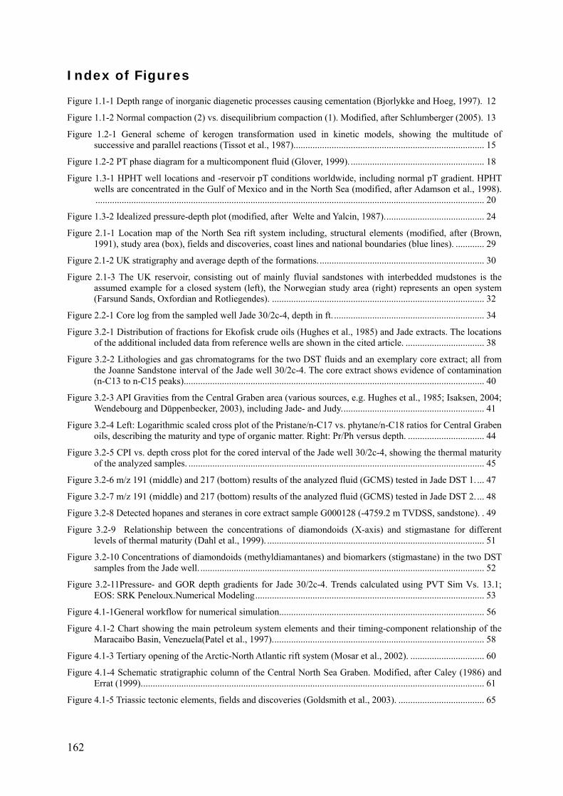
Index of Figures

12 Figure 1.1-1 Depth range of inorganic diagenetic processes causing cementation (Bjorlykke and Hoeg, 1997).

13 Figure 1.1-2 Normal compaction (2) vs. disequilibrium compaction (1). Modified, after Schlumberger (2005).

Figure 1.2-1 General scheme of kerogen transformation used in kinetic models, showing the multitude of successive and parallel reactions (Tissot et al., 1987)................................................................................ 15

........................................................ 18 Figure 1.2-2 PT phase diagram for a multicomponent fluid (Glover, 1999).

Figure 1.3-1 HPHT well locations and -reservoir pT conditions worldwide, including normal pT gradient. HPHT wells are concentrated in the Gulf of Mexico and in the North Sea (modified, after Adamson et al., 1998).................................................................................................................................................................... 20

......................................... 24 Figure 1.3-2 Idealized pressure-depth plot (modified, after Welte and Yalcin, 1987).

Figure 2.1-1 Location map of the North Sea rift system including, structural elements (modified, after (Brown, 1991), study area (box), fields and discoveries, coast lines and national boundaries (blue lines). ............ 29

..................................................................... 30 Figure 2.1-2 UK stratigraphy and average depth of the formations.

Figure 2.1-3 The UK reservoir, consisting out of mainly fluvial sandstones with interbedded mudstones is the assumed example for a closed system (left), the Norwegian study area (right) represents an open system (Farsund Sands, Oxfordian and Rotliegendes). ......................................................................................... 32

............................................................... 34 Figure 2.2-1 Core log from the sampled well Jade 30/2c-4, depth in ft.

Figure 3.2-1 Distribution of fractions for Ekofisk crude oils (Hughes et al., 1985) and Jade extracts. The locations of the additional included data from reference wells are shown in the cited article. ................................. 38

Figure 3.2-2 Lithologies and gas chromatograms for the two DST fluids and an exemplary core extract; all from the Joanne Sandstone interval of the Jade well 30/2c-4. The core extract shows evidence of contamination (n-C13 to n-C15 peaks).............................................................................................................................. 40

Figure 3.2-3 API Gravities from the Central Graben area (various sources, e.g. Hughes et al., 1985; Isaksen, 2004; Wendebourg and Düppenbecker, 2003), including Jade- and Judy............................................................ 41

Figure 3.2-4 Left: Logarithmic scaled cross plot of the Pristane/n-C17 vs. phytane/n-C18 ratios for Central Graben oils, describing the maturity and type of organic matter. Right: Pr/Ph versus depth. ................................ 44

Figure 3.2-5 CPI vs. depth cross plot for the cored interval of the Jade well 30/2c-4, showing the thermal maturity of the analyzed samples. ............................................................................................................................ 45

... 47 Figure 3.2-6 m/z 191 (middle) and 217 (bottom) results of the analyzed fluid (GCMS) tested in Jade DST 1.

... 48 Figure 3.2-7 m/z 191 (middle) and 217 (bottom) results of the analyzed fluid (GCMS) tested in Jade DST 2.

. 49 Figure 3.2-8 Detected hopanes and steranes in core extract sample G000128 (-4759.2 m TVDSS, sandstone).

Figure 3.2-9 Relationship between the concentrations of diamondoids (X-axis) and stigmastane for different levels of thermal maturity (Dahl et al., 1999). ........................................................................................... 51

Figure 3.2-10 Concentrations of diamondoids (methyldiamantanes) and biomarkers (stigmastane) in the two DST samples from the Jade well. ....................................................................................................................... 52

Figure 3.2-11Pressure- and GOR depth gradients for Jade 30/2c-4. Trends calculated using PVT Sim Vs. 13.1; EOS: SRK Peneloux.Numerical Modeling................................................................................................ 53

Figure 4.1-1General workflow for numerical simulation...................................................................................... 56 Figure 4.1-2 Chart showing the main petroleum system elements and their timing-component relationship of the

Maracaibo Basin, Venezuela(Patel et al., 1997)......................................................................................... 58 ............................... 60 Figure 4.1-3 Tertiary opening of the Arctic-North Atlantic rift system (Mosar et al., 2002).

Figure 4.1-4 Schematic stratigraphic column of the Central North Sea Graben. Modified, after Caley (1986) and Errat (1999)................................................................................................................................................ 61

.................................... 65 Figure 4.1-5 Triassic tectonic elements, fields and discoveries (Goldsmith et al., 2003).

162

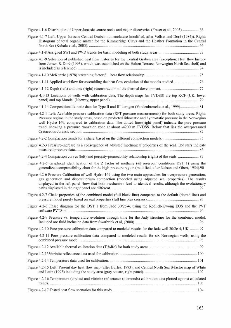
................ 66 Figure 4.1-6 Distribution of Upper Jurassic source rocks and major discoveries (Fraser et al., 2003).

Figure 4.1-7 Left: Upper Jurassic Central Graben nomenclature (modified, after Vollset and Doré (1984)). Right: Histogram of total organic matter for the Kimmeridge Clays and the Heather Formation in the Central North Sea (Kubala et al., 2003). ................................................................................................................ 66

......................................... 73 Figure 4.1-8 Assigned SWI and PWD trends for basin modeling of both study areas.

Figure 4.1-9 Selection of published heat flow histories for the Central Graben area (exception: Heat flow history from Jensen & Doré (1993), which was established on the Halten Terrace, Norwegian North Sea shelf, and is included as reference). ........................................................................................................................... 74

...................................................... 75 Figure 4.1-10 McKenzie (1978) stretching factor β – heat flow relationship.

......................... 76 Figure 4.1-11 Applied workflow for assembling the heat flow evolution of the models studied.

...................................... 77 Figure 4.1-12 Depth (left) and time (right) reconstruction of the thermal development.

Figure 4.1-13 Locations of wells with calibration data. The depth maps (m TVDSS) are top KCF (UK, lower panel) and top Mandal (Norway, upper panel)........................................................................................... 79

.................. 81 Figure 4.1-14 Compositional kinetic data for Type II and III kerogen (Vandenbroucke et al., 1999).

Figure 4.2-1 Left: Available pressure calibration data (RFT pressure measurements) for both study areas. Right: Pressure regime in the study areas, based on predicted lithostatic and hydrostatic pressure in the Norwegian well Hydro 169, compared to calibration data. The dotted lines(right panel) indicate the pore pressure trend, showing a pressure transition zone at about -4200 m TVDSS. Below that lies the overpressured Cretaceous-Jurassic section. ...................................................................................................................... 82

..................................... 85 Figure 4.2-2 Compaction trends for a shale, based on the different compaction models.

Figure 4.2-3 Pressure-increase as a consequence of adjusted mechanical properties of the seal. The stars indicate measured pressure data. ............................................................................................................................. 86

..................... 87 Figure 4.2-4 Compaction curves (left) and porosity-permeability relationship (right) of the seals.

Figure 4.2-5 Graphical identification of the Z factor of methane (@ reservoir conditions DST 1) using the generalized compressibility chart for the high-pressure region (modified, after Nelson and Obert, 1954).90

Figure 4.2-6 Pressure Calibration of well Hydro 169 using the two main approaches for overpressure generation, gas generation and disequilibrium compaction (modeled using adjusted seal properties). The results displayed in the left panel show that both mechanism lead to identical results, although the evolutionary paths displayed in the right panel are different. ......................................................................................... 92

Figure 4.2-7 Chalk properties of the combined model (full black line) compared to the default (dotted line) and pressure model purely based on seal properties (full line plus crosses)..................................................... 93

Figure 4.2-8 Phase diagram for the DST 1 from Jade 30/2c-4, using the Redlich-Kwong EOS and the PVT software PVTSim....................................................................................................................................... 94

Figure 4.2-9 Pressure vs. temperature evolution through time for the Judy structure for the combined model. Included are fluid inclusion data from Swarbrick et al, (2000). ................................................................ 96

......... 97 Figure 4.2-10 Pore pressure calibration data compared to modeled results for the Jade well 30/2c-4, UK.

Figure 4.2-11 Pore pressure calibration data compared to modeled results for six Norwegian wells, using the combined pressure model. ......................................................................................................................... 98

.................................................. 99 Figure 4.2-12 Available thermal calibration data (T,%Ro) for both study areas.

............................................................................... 100 Figure 4.2-13Vitrinite reflectance data used for calibration.

......................................................................................... 101 Figure 4.2-14 Temperature data used for calibration.

Figure 4.2-15 Left: Present day heat flow map (after Burley, 1993), and Central North Sea β-factor map of White and Latin (1993) including the study area (gray square, right panel). ..................................................... 102

Figure 4.2-16 Temperature (circles) and vitrinite reflectance (diamonds) calibration data plotted against calculated trends. ...................................................................................................................................................... 103

..................................................................................... 104 Figure 4.2-17 Tested heat flow scenarios for this study.

163

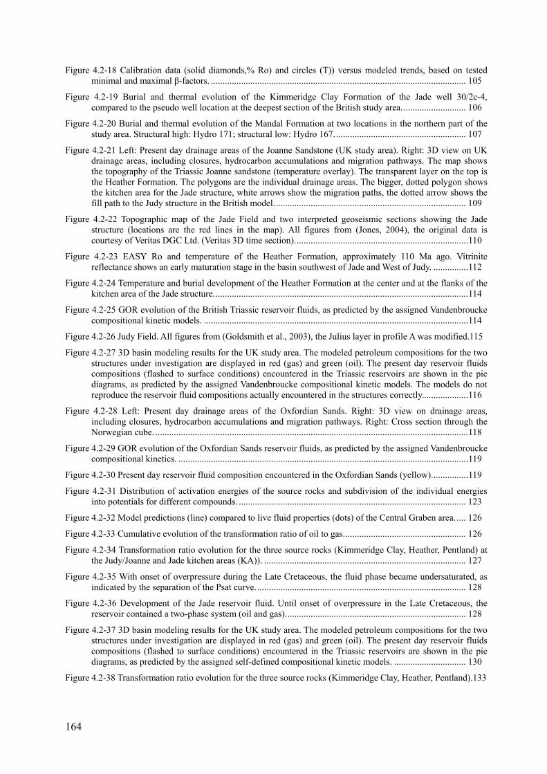
Figure 4.2-18 Calibration data (solid diamonds,% Ro) and circles (T)) versus modeled trends, based on tested minimal and maximal β-factors. .............................................................................................................. 105

Figure 4.2-19 Burial and thermal evolution of the Kimmeridge Clay Formation of the Jade well 30/2c-4, compared to the pseudo well location at the deepest section of the British study area............................ 106

Figure 4.2-20 Burial and thermal evolution of the Mandal Formation at two locations in the northern part of the study area. Structural high: Hydro 171; structural low: Hydro 167......................................................... 107

Figure 4.2-21 Left: Present day drainage areas of the Joanne Sandstone (UK study area). Right: 3D view on UK drainage areas, including closures, hydrocarbon accumulations and migration pathways. The map shows the topography of the Triassic Joanne sandstone (temperature overlay). The transparent layer on the top is the Heather Formation. The polygons are the individual drainage areas. The bigger, dotted polygon shows the kitchen area for the Jade structure, white arrows show the migration paths, the dotted arrow shows the fill path to the Judy structure in the British model................................................................................... 109

Figure 4.2-22 Topographic map of the Jade Field and two interpreted geoseismic sections showing the Jade structure (locations are the red lines in the map). All figures from (Jones, 2004), the original data is courtesy of Veritas DGC Ltd. (Veritas 3D time section)...........................................................................110

Figure 4.2-23 EASY Ro and temperature of the Heather Formation, approximately 110 Ma ago. Vitrinite reflectance shows an early maturation stage in the basin southwest of Jade and West of Judy. ...............112

Figure 4.2-24 Temperature and burial development of the Heather Formation at the center and at the flanks of the kitchen area of the Jade structure..............................................................................................................114

Figure 4.2-25 GOR evolution of the British Triassic reservoir fluids, as predicted by the assigned Vandenbroucke compositional kinetic models. ..................................................................................................................114

Figure 4.2-26 Judy Field. All figures from (Goldsmith et al., 2003), the Julius layer in profile A was modified.115 Figure 4.2-27 3D basin modeling results for the UK study area. The modeled petroleum compositions for the two

structures under investigation are displayed in red (gas) and green (oil). The present day reservoir fluids compositions (flashed to surface conditions) encountered in the Triassic reservoirs are shown in the pie diagrams, as predicted by the assigned Vandenbroucke compositional kinetic models. The models do not reproduce the reservoir fluid compositions actually encountered in the structures correctly....................116

Figure 4.2-28 Left: Present day drainage areas of the Oxfordian Sands. Right: 3D view on drainage areas, including closures, hydrocarbon accumulations and migration pathways. Right: Cross section through the Norwegian cube. .......................................................................................................................................118

Figure 4.2-29 GOR evolution of the Oxfordian Sands reservoir fluids, as predicted by the assigned Vandenbroucke compositional kinetics. .............................................................................................................................119

...............119 Figure 4.2-30 Present day reservoir fluid composition encountered in the Oxfordian Sands (yellow).

Figure 4.2-31 Distribution of activation energies of the source rocks and subdivision of the individual energies into potentials for different compounds. .................................................................................................. 123

.... 126 Figure 4.2-32 Model predictions (line) compared to live fluid properties (dots) of the Central Graben area.

.................................................... 126 Figure 4.2-33 Cumulative evolution of the transformation ratio of oil to gas.

Figure 4.2-34 Transformation ratio evolution for the three source rocks (Kimmeridge Clay, Heather, Pentland) at the Judy/Joanne and Jade kitchen areas (KA)). ....................................................................................... 127

Figure 4.2-35 With onset of overpressure during the Late Cretaceous, the fluid phase became undersaturated, as indicated by the separation of the Psat curve. .......................................................................................... 128

Figure 4.2-36 Development of the Jade reservoir fluid. Until onset of overpressure in the Late Cretaceous, the reservoir contained a two-phase system (oil and gas).............................................................................. 128

Figure 4.2-37 3D basin modeling results for the UK study area. The modeled petroleum compositions for the two structures under investigation are displayed in red (gas) and green (oil). The present day reservoir fluids compositions (flashed to surface conditions) encountered in the Triassic reservoirs are shown in the pie diagrams, as predicted by the assigned self-defined compositional kinetic models. ............................... 130

Figure 4.2-38 Transformation ratio evolution for the three source rocks (Kimmeridge Clay, Heather, Pentland).133

164

Figure 4.2-39 With the onset of overpressure in the Late Cretaceous to Early Eocene, the fluid phase became undersaturated, as indicated by the separation of the Psat curve. Phase separation occurred distinctively later than in the Triassic UK reservoirs.................................................................................................... 133

Figure 4.2-40 GOR development in the Oxfordian sands. The increase of the GOR of the fluids is linked to accelerated burial, coupled with further source rock maturation. ............................................................ 134

Figure 4.2-41 In the Norwegian Oxfordian reservoirs temperatures above 80°C at first fluid emplacement precluded the risk of significant biodegradation...................................................................................... 134

Figure 4.2-42 Present day reservoir fluid composition encountered in the Oxfordian Sands (yellow) prospect (hydrocarbon accumulation in green). ..................................................................................................... 136

165

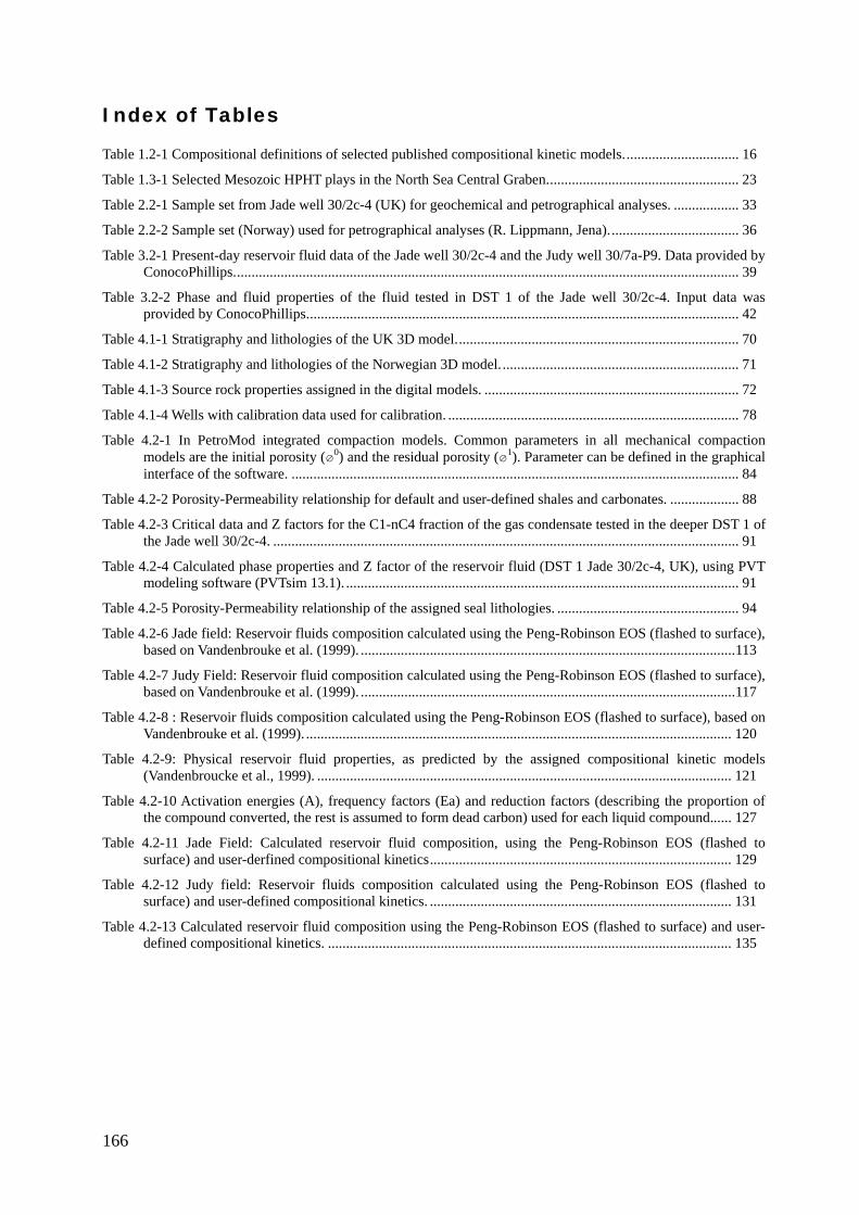
166

Index of Tables

Table 1.2-1 Compositional definitions of selected published compositional kinetic models................................ 16 Table 1.3-1 Selected Mesozoic HPHT plays in the North Sea Central Graben..................................................... 23 Table 2.2-1 Sample set from Jade well 30/2c-4 (UK) for geochemical and petrographical analyses. .................. 33 Table 2.2-2 Sample set (Norway) used for petrographical analyses (R. Lippmann, Jena).................................... 36 Table 3.2-1 Present-day reservoir fluid data of the Jade well 30/2c-4 and the Judy well 30/7a-P9. Data provided by

ConocoPhillips........................................................................................................................................... 39 Table 3.2-2 Phase and fluid properties of the fluid tested in DST 1 of the Jade well 30/2c-4. Input data was

provided by ConocoPhillips....................................................................................................................... 42 Table 4.1-1 Stratigraphy and lithologies of the UK 3D model.............................................................................. 70 Table 4.1-2 Stratigraphy and lithologies of the Norwegian 3D model.................................................................. 71 Table 4.1-3 Source rock properties assigned in the digital models. ...................................................................... 72 Table 4.1-4 Wells with calibration data used for calibration. ................................................................................ 78 Table 4.2-1 In PetroMod integrated compaction models. Common parameters in all mechanical compaction

models are the initial porosity (i0) and the residual porosity (i1). Parameter can be defined in the graphical interface of the software. ........................................................................................................................... 84

Table 4.2-2 Porosity-Permeability relationship for default and user-defined shales and carbonates. ................... 88 Table 4.2-3 Critical data and Z factors for the C1-nC4 fraction of the gas condensate tested in the deeper DST 1 of

the Jade well 30/2c-4. ................................................................................................................................ 91 Table 4.2-4 Calculated phase properties and Z factor of the reservoir fluid (DST 1 Jade 30/2c-4, UK), using PVT

modeling software (PVTsim 13.1). ............................................................................................................ 91 Table 4.2-5 Porosity-Permeability relationship of the assigned seal lithologies. .................................................. 94 Table 4.2-6 Jade field: Reservoir fluids composition calculated using the Peng-Robinson EOS (flashed to surface),

based on Vandenbrouke et al. (1999). .......................................................................................................113 Table 4.2-7 Judy Field: Reservoir fluid composition calculated using the Peng-Robinson EOS (flashed to surface),

based on Vandenbrouke et al. (1999). .......................................................................................................117 Table 4.2-8 : Reservoir fluids composition calculated using the Peng-Robinson EOS (flashed to surface), based on

Vandenbrouke et al. (1999). ..................................................................................................................... 120 Table 4.2-9: Physical reservoir fluid properties, as predicted by the assigned compositional kinetic models

(Vandenbroucke et al., 1999). .................................................................................................................. 121 Table 4.2-10 Activation energies (A), frequency factors (Ea) and reduction factors (describing the proportion of

the compound converted, the rest is assumed to form dead carbon) used for each liquid compound...... 127 Table 4.2-11 Jade Field: Calculated reservoir fluid composition, using the Peng-Robinson EOS (flashed to

surface) and user-derfined compositional kinetics................................................................................... 129 Table 4.2-12 Judy field: Reservoir fluids composition calculated using the Peng-Robinson EOS (flashed to

surface) and user-defined compositional kinetics. ................................................................................... 131 Table 4.2-13 Calculated reservoir fluid composition using the Peng-Robinson EOS (flashed to surface) and user-

defined compositional kinetics. ............................................................................................................... 135

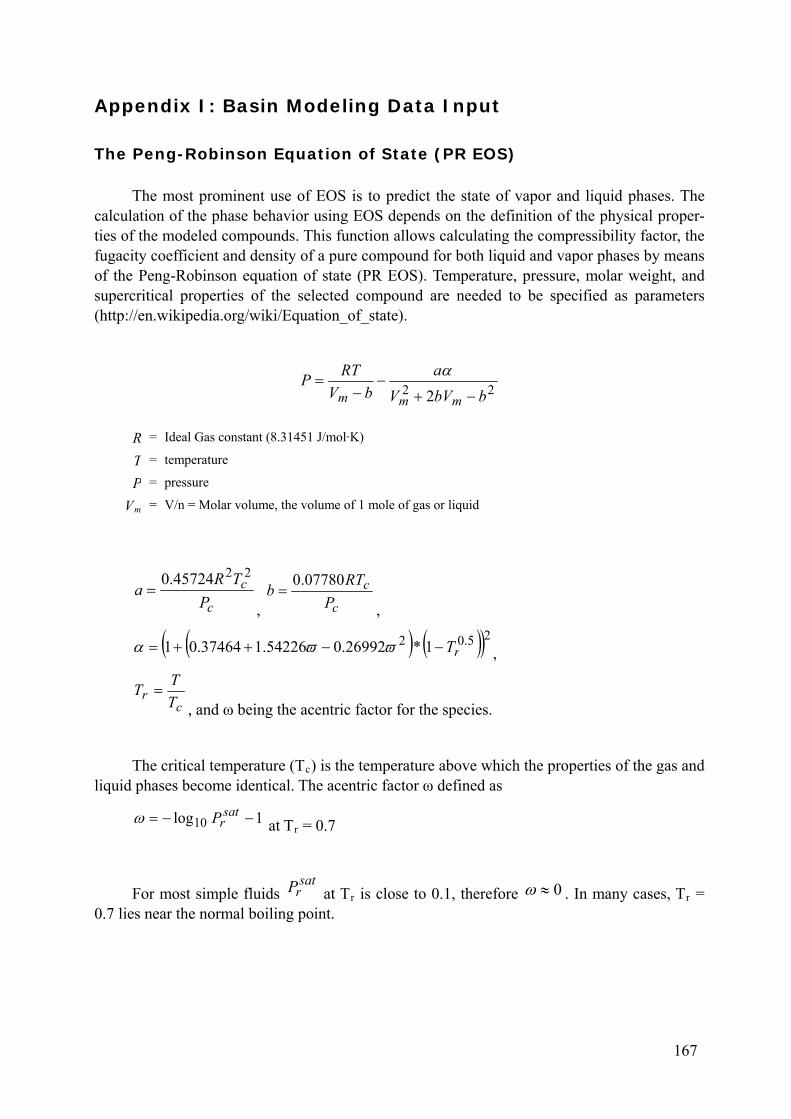
Appendix I: Basin Modeling Data Input

The Peng-Robinson Equation of State (PR EOS)

The most prominent use of EOS is to predict the state of vapor and liquid phases. The calculation of the phase behavior using EOS depends on the definition of the physical proper-ties of the modeled compounds. This function allows calculating the compressibility factor, the fugacity coefficient and density of a pure compound for both liquid and vapor phases by means of the Peng-Robinson equation of state (PR EOS). Temperature, pressure, molar weight, and supercritical properties of the selected compound are needed to be specified as parameters (http://en.wikipedia.org/wiki/Equation_of_state).

22 2 bbVVa

bVRTP

mmm −+−

−=

α

R = Ideal Gas constant (8.31451 J/mol·K)

T = temperature

P = pressure

V = V/n = Molar volume, the volume of 1 mole of gas or liquid m

c

cP

TRa

2245724.0=

c

cP

RTb

07780.0=

, ,

( ) ( )( )25.02 1*26992.054226.137464.01 rT−−++= ϖϖα ,

cr T

TT =, and ω being the acentric factor for the species.

The critical temperature (Tc) is the temperature above which the properties of the gas and liquid phases become identical. The acentric factor ω defined as

1log10 −−= satrPω at T = 0.7 r

For most simple fluids tsa

rP e is close to 0.1, therefor 0≈ω at T . In many cases, Tr r = 0.7 lies near the normal boiling point.

167

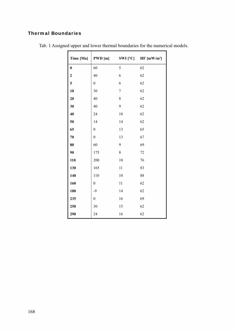
Thermal Boundaries

Tab. 1 Assigned upper and lower thermal boundaries for the numerical models.

Time [Ma] PWD [m] SWI [°C] HF [mW/m²]

0 60 5 62

2 40 6 62

5 0 6 62

10 30 7 62

20 40 8 62

30 40 9 62

40 24 10 62

50 14 14 62

65 0 13 65

70 0 13 67

80 60 9 69

90 175 8 72

110 200 10 76

130 165 11 83

140 110 10 88

160 0 11 62

180 -9 14 62

235 0 16 69

250 30 15 62

290 24 16 62

168

Appendix II: Compositional Kinetic Models

In addition to the characterization of primary cracking products, described by the compo-sitional kinetic models, secondary cracking of the primary generated compounds was also de-fined. The secondary cracking of hydrocarbons was investigated experimentally in detail (Horsfield et al., 1992, Schenk et al., 1997, Dieckmann et al., 1998).

While the stability of hydrocarbons in reservoirs is relatively high, onset of in-reservoir cracking starts at reservoir temperatures of 180-200°C at geologic heating rates (Horsfield et al., 1992, Schenk et al., 1997), cracking of residual hydrocarbons in the source rock environ-ment occurs at significantly lower geologic temperatures, i.e. starting already at roughly 150°C (Dieckmann et al., 1998). In the experimental studies listed oil cracking was described by the formation of gas (C1-5) due to the cracking of the C6+ petroleum fraction.

For the compositional kinetic models applied in this study the use of 7 compounds de-scribing the liquid composition precluded the definition of oil cracking using a single bulk re-action characterization.

In order to define oil to gas cracking, the stability of the liquid fractions was varied sys-tematically within the stability framework defined by the in-reservoir and in-source oil to gas cracking kinetics of Schenk et al. (1997) and Dieckmann et al. (1998). Activation energies, frequency factors and reduction factors (describing the proportion of the compound converted, the rest is assumed to form dead carbon) used for each liquid compound are shown in Table 2 and 3, the cumulative evolution of oil to gas for three compounds is shown in Figure 4.2-38 and compared to transformation ratios of the Dieckmann et al. (1998) and Schenk et al. (1997) oil to gas kinetics.

Methane was defined as the single compound being produced from oil cracking.

169

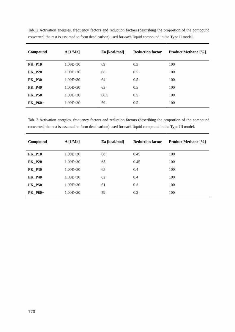
170

Tab. 2 Activation energies, frequency factors and reduction factors (describing the proportion of the compound

converted, the rest is assumed to form dead carbon) used for each liquid compound in the Type II model.

Compound A [1/Ma] Ea [kcal/mol] Reduction factor Product Methane [%]

PK_P10 1.00E+30 69 0.5 100

PK_P20 1.00E+30 66 0.5 100

PK_P30 1.00E+30 64 0.5 100

PK_P40 1.00E+30 63 0.5 100

PK_P50 1.00E+30 60.5 0.5 100

PK_P60+ 1.00E+30 59 0.5 100

Tab. 3 Activation energies, frequency factors and reduction factors (describing the proportion of the compound

converted, the rest is assumed to form dead carbon) used for each liquid compound in the Type III model.

Compound A [1/Ma] Ea [kcal/mol] Reduction factor Product Methane [%]

PK_P10 1.00E+30 68 0.45 100

PK_P20 1.00E+30 65 0.45 100

PK_P30 1.00E+30 63 0.4 100

PK_P40 1.00E+30 62 0.4 100

PK_P50 1.00E+30 61 0.3 100

PK_P60+ 1.00E+30 59 0.3 100

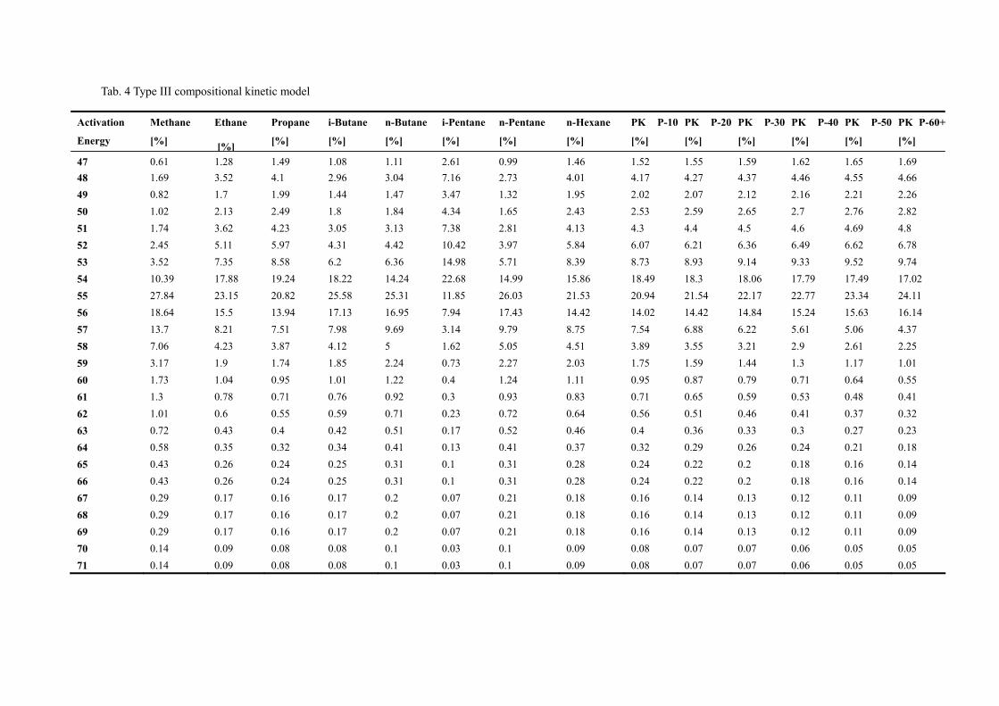
Tab. 4 Type III compositional kinetic model

Activation

Energy

Methane

[%]

Ethane

[%]

Propane

[%]

i-Butane

[%]

n-Butane

[%]

i-Pentane

[%]

n-Pentane

[%]

n-Hexane

[%]

PK P-10

[%]

PK P-20

[%]

PK P-30

[%]

PK P-40

[%]

PK P-50

[%]

PK P-60+

[%]

47 0.61 1.28 1.49 1.08 1.11 2.61 0.99 1.46 1.52 1.55 1.59 1.62 1.65 1.69 48 1.69 3.52 4.1 2.96 3.04 7.16 2.73 4.01 4.17 4.27 4.37 4.46 4.55 4.66 49 0.82 1.7 1.99 1.44 1.47 3.47 1.32 1.95 2.02 2.07 2.12 2.16 2.21 2.26 50 1.02 2.13 2.49 1.8 1.84 4.34 1.65 2.43 2.53 2.59 2.65 2.7 2.76 2.82 51 1.74 3.62 4.23 3.05 3.13 7.38 2.81 4.13 4.3 4.4 4.5 4.6 4.69 4.8 52 2.45 5.11 5.97 4.31 4.42 10.42 3.97 5.84 6.07 6.21 6.36 6.49 6.62 6.78 53 3.52 7.35 8.58 6.2 6.36 14.98 5.71 8.39 8.73 8.93 9.14 9.33 9.52 9.74 54 10.39 17.88 19.24 18.22 14.24 22.68 14.99 15.86 18.49 18.3 18.06 17.79 17.49 17.02 55 27.84 23.15 20.82 25.58 25.31 11.85 26.03 21.53 20.94 21.54 22.17 22.77 23.34 24.11 56 18.64 15.5 13.94 17.13 16.95 7.94 17.43 14.42 14.02 14.42 14.84 15.24 15.63 16.14 57 13.7 8.21 7.51 7.98 9.69 3.14 9.79 8.75 7.54 6.88 6.22 5.61 5.06 4.37 58 7.06 4.23 3.87 4.12 5 1.62 5.05 4.51 3.89 3.55 3.21 2.9 2.61 2.25 59 3.17 1.9 1.74 1.85 2.24 0.73 2.27 2.03 1.75 1.59 1.44 1.3 1.17 1.01 60 1.73 1.04 0.95 1.01 1.22 0.4 1.24 1.11 0.95 0.87 0.79 0.71 0.64 0.55 61 1.3 0.78 0.71 0.76 0.92 0.3 0.93 0.83 0.71 0.65 0.59 0.53 0.48 0.41 62 1.01 0.6 0.55 0.59 0.71 0.23 0.72 0.64 0.56 0.51 0.46 0.41 0.37 0.32 63 0.72 0.43 0.4 0.42 0.51 0.17 0.52 0.46 0.4 0.36 0.33 0.3 0.27 0.23 64 0.58 0.35 0.32 0.34 0.41 0.13 0.41 0.37 0.32 0.29 0.26 0.24 0.21 0.18 65 0.43 0.26 0.24 0.25 0.31 0.1 0.31 0.28 0.24 0.22 0.2 0.18 0.16 0.14 66 0.43 0.26 0.24 0.25 0.31 0.1 0.31 0.28 0.24 0.22 0.2 0.18 0.16 0.14 67 0.29 0.17 0.16 0.17 0.2 0.07 0.21 0.18 0.16 0.14 0.13 0.12 0.11 0.09 68 0.29 0.17 0.16 0.17 0.2 0.07 0.21 0.18 0.16 0.14 0.13 0.12 0.11 0.09 69 0.29 0.17 0.16 0.17 0.2 0.07 0.21 0.18 0.16 0.14 0.13 0.12 0.11 0.09 70 0.14 0.09 0.08 0.08 0.1 0.03 0.1 0.09 0.08 0.07 0.07 0.06 0.05 0.05 71 0.14 0.09 0.08 0.08 0.1 0.03 0.1 0.09 0.08 0.07 0.07 0.06 0.05 0.05

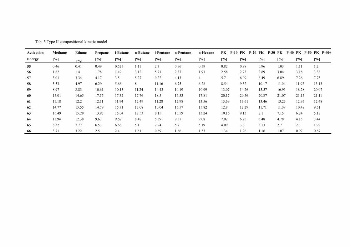
Tab. 5 Type II compositional kinetic model

Propane

[%]

i-Butane

[%]

n-Butane

[%]

i-Pentane

[%]

n-Pentane

[%]

n-Hexane

[%]

PK P-10

[%]

PK P-20

[%]

PK P-30

[%]

PK P-40

[%]

PK P-50

[%]

PK P-60+

[%]

Activation

Energy

Methane

[%]

Ethane

[%] 0.46 0.41 0.49 0.525 1.11 2.3 0.96 0.59 0.82 0.88 0.96 1.03 1.11 1.2 55 1.62 1.4 1.78 1.49 3.12 5.71 2.37 1.91 2.58 2.73 2.89 3.04 3.18 3.36 56 3.01 3.34 4.17 3.5 5.27 9.22 4.13 4 5.7 6.09 6.49 6.89 7.26 7.73 57 5.53 4.97 6.29 5.66 8 11.16 6.75 6.28 8.54 9.32 10.17 11.04 11.92 13.13 58 8.97 8.83 10.61 10.13 11.24 14.43 10.19 10.99 13.07 14.26 15.57 16.91 18.28 20.07 59 15.01 14.65 17.15 17.32 17.76 18.5 16.53 17.81 20.17 20.56 20.87 21.07 21.15 21.11 60 11.18 12.2 12.11 11.94 12.49 11.28 12.98 13.56 13.69 13.61 13.46 13.23 12.95 12.48 61 14.77 15.55 14.79 15.71 13.08 10.04 15.57 15.82 12.8 12.29 11.71 11.09 10.48 9.51 62 15.49 15.28 13.93 15.04 12.53 8.15 13.59 13.24 10.16 9.13 8.1 7.15 6.24 5.18 63 11.94 12.38 9.67 9.62 8.48 5.39 9.37 9.08 7.02 6.25 5.48 4.78 4.15 3.44 64 8.32 7.77 6.53 6.66 5.1 2.94 5.7 5.19 4.09 3.6 3.13 2.7 2.3 1.92 65 3.71 3.22 2.5 2.4 1.81 0.89 1.86 1.53 1.34 1.26 1.16 1.07 0.97 0.87 66

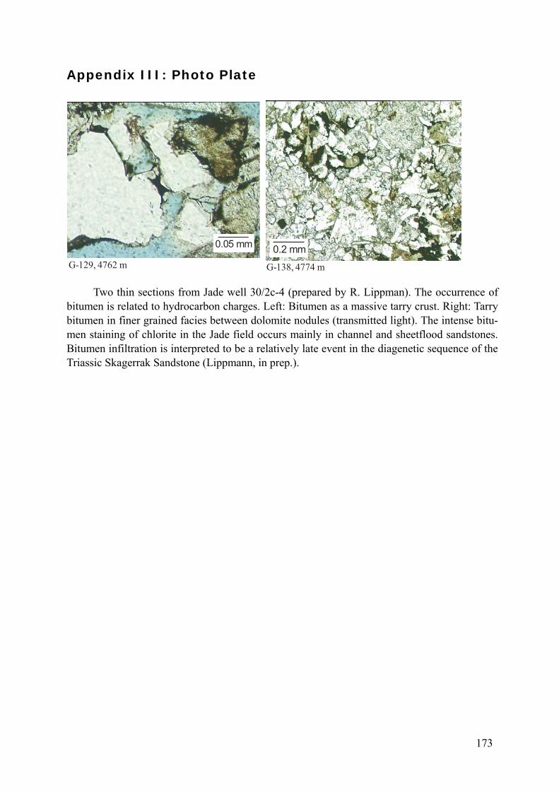
Appendix III: Photo Plate

0.05 mm 0.2 mm

G-138, 4774 mG-129, 4762 m

Two thin sections from Jade well 30/2c-4 (prepared by R. Lippman). The occurrence of bitumen is related to hydrocarbon charges. Left: Bitumen as a massive tarry crust. Right: Tarry bitumen in finer grained facies between dolomite nodules (transmitted light). The intense bitu-men staining of chlorite in the Jade field occurs mainly in channel and sheetflood sandstones. Bitumen infiltration is interpreted to be a relatively late event in the diagenetic sequence of the Triassic Skagerrak Sandstone (Lippmann, in prep.).

173

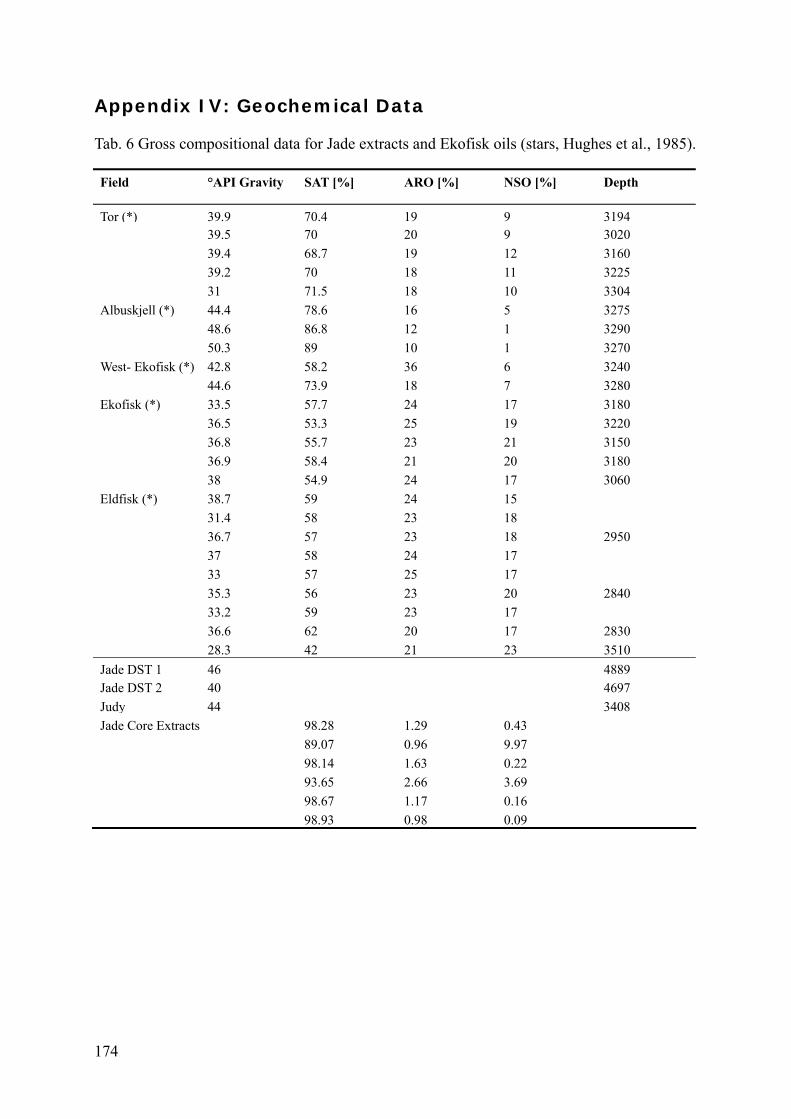
Appendix IV: Geochemical Data

Tab. 6 Gross compositional data for Jade extracts and Ekofisk oils (stars, Hughes et al., 1985).

Field °API Gravity SAT [%] ARO [%] NSO [%] Depth

Tor (*) 39.9 70.4 19 9 3194 39.5 70 20 9 3020 39.4 68.7 19 12 3160 39.2 70 18 11 3225 31 71.5 18 10 3304 Albuskjell (*) 44.4 78.6 16 5 3275 48.6 86.8 12 1 3290 50.3 89 10 1 3270 West- Ekofisk (*) 42.8 58.2 36 6 3240 44.6 73.9 18 7 3280 Ekofisk (*) 33.5 57.7 24 17 3180 36.5 53.3 25 19 3220 36.8 55.7 23 21 3150 36.9 58.4 21 20 3180 38 54.9 24 17 3060 Eldfisk (*) 38.7 59 24 15 31.4 58 23 18 36.7 57 23 18 2950 37 58 24 17 33 57 25 17 35.3 56 23 20 2840 33.2 59 23 17 36.6 62 20 17 2830 28.3 42 21 23 3510 Jade DST 1 46 4889 Jade DST 2 40 4697 Judy 44 3408 Jade Core Extracts 98.28 1.29 0.43 89.07 0.96 9.97 98.14 1.63 0.22 93.65 2.66 3.69 98.67 1.17 0.16 98.93 0.98 0.09

174

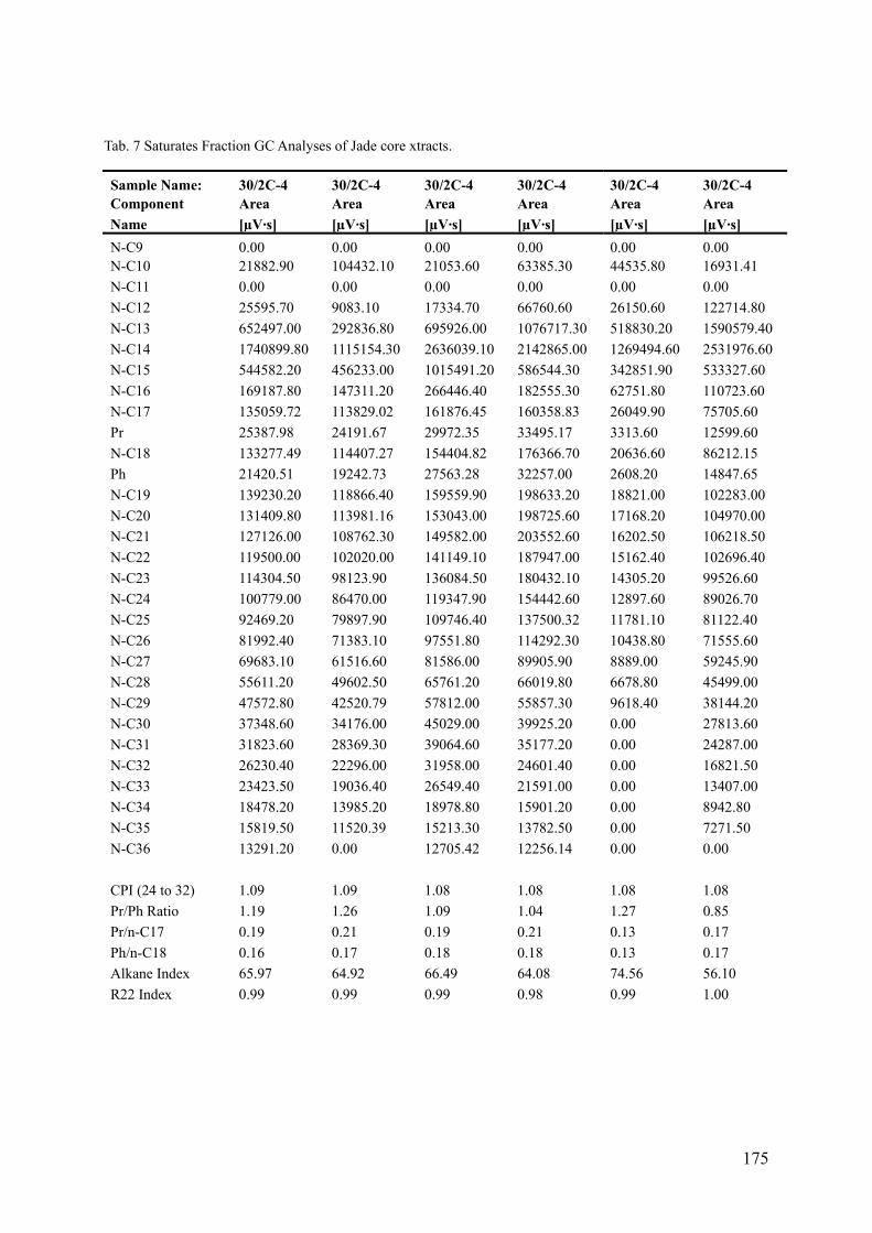
Tab. 7 Saturates Fraction GC Analyses of Jade core xtracts.

Sample Name: 30/2C-4 30/2C-4 30/2C-4 30/2C-4 30/2C-4 30/2C-4 Component Area Area Area Area Area AreaName [µV·s] [µV·s] [µV·s] [µV·s] [µV·s] [µV·s]N-C9 0.00 0.00 0.00 0.00 0.00 0.00N-C10 21882.90 104432.10 21053.60 63385.30 44535.80 16931.41N-C11 0.00 0.00 0.00 0.00 0.00 0.00N-C12 25595.70 9083.10 17334.70 66760.60 26150.60 122714.80N-C13 652497.00 292836.80 695926.00 1076717.30 518830.20 1590579.40N-C14 1740899.80 1115154.30 2636039.10 2142865.00 1269494.60 2531976.60N-C15 544582.20 456233.00 1015491.20 586544.30 342851.90 533327.60N-C16 169187.80 147311.20 266446.40 182555.30 62751.80 110723.60N-C17 135059.72 113829.02 161876.45 160358.83 26049.90 75705.60Pr 25387.98 24191.67 29972.35 33495.17 3313.60 12599.60N-C18 133277.49 114407.27 154404.82 176366.70 20636.60 86212.15Ph 21420.51 19242.73 27563.28 32257.00 2608.20 14847.65N-C19 139230.20 118866.40 159559.90 198633.20 18821.00 102283.00N-C20 131409.80 113981.16 153043.00 198725.60 17168.20 104970.00N-C21 127126.00 108762.30 149582.00 203552.60 16202.50 106218.50N-C22 119500.00 102020.00 141149.10 187947.00 15162.40 102696.40N-C23 114304.50 98123.90 136084.50 180432.10 14305.20 99526.60N-C24 100779.00 86470.00 119347.90 154442.60 12897.60 89026.70N-C25 92469.20 79897.90 109746.40 137500.32 11781.10 81122.40N-C26 81992.40 71383.10 97551.80 114292.30 10438.80 71555.60N-C27 69683.10 61516.60 81586.00 89905.90 8889.00 59245.90N-C28 55611.20 49602.50 65761.20 66019.80 6678.80 45499.00N-C29 47572.80 42520.79 57812.00 55857.30 9618.40 38144.20N-C30 37348.60 34176.00 45029.00 39925.20 0.00 27813.60N-C31 31823.60 28369.30 39064.60 35177.20 0.00 24287.00N-C32 26230.40 22296.00 31958.00 24601.40 0.00 16821.50N-C33 23423.50 19036.40 26549.40 21591.00 0.00 13407.00N-C34 18478.20 13985.20 18978.80 15901.20 0.00 8942.80N-C35 15819.50 11520.39 15213.30 13782.50 0.00 7271.50N-C36 13291.20 0.00 12705.42 12256.14 0.00 0.00 CPI (24 to 32) 1.09 1.09 1.08 1.08 1.08 1.08Pr/Ph Ratio 1.19 1.26 1.09 1.04 1.27 0.85Pr/n-C17 0.19 0.21 0.19 0.21 0.13 0.17Ph/n-C18 0.16 0.17 0.18 0.18 0.13 0.17Alkane Index 65.97 64.92 66.49 64.08 74.56 56.10R22 Index 0.99 0.99 0.99 0.98 0.99 1.00

175

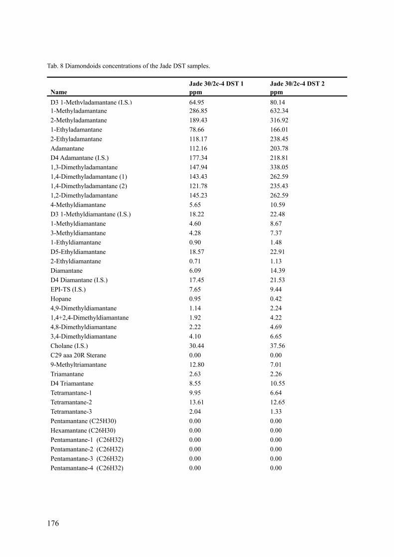
Tab. 8 Diamondoids concentrations of the Jade DST samples.

Jade 30/2c-4 DST 1 Jade 30/2c-4 DST 2 Name ppm ppm D3 1-Methyladamantane (I.S.) 64.95 80.14 1-Methyladamantane 286.85 632.34 2-Methyladamantane 189.43 316.92 1-Ethyladamantane 78.66 166.01 2-Ethyladamantane 118.17 238.45 Adamantane 112.16 203.78 D4 Adamantane (I.S.) 177.34 218.81 1,3-Dimethyladamantane 147.94 338.05 1,4-Dimethyladamantane (1) 143.43 262.59 1,4-Dimethyladamantane (2) 121.78 235.43 1,2-Dimethyladamantane 145.23 262.59 4-Methyldiamantane 5.65 10.59 D3 1-Methyldiamantane (I.S.) 18.22 22.48 1-Methyldiamantane 4.60 8.67 3-Methyldiamantane 4.28 7.37 1-Ethyldiamantane 0.90 1.48 D5-Ethyldiamantane 18.57 22.91 2-Ethyldiamantane 0.71 1.13 Diamantane 6.09 14.39 D4 Diamantane (I.S.) 17.45 21.53 EPI-TS (I.S.) 7.65 9.44 Hopane 0.95 0.42 4,9-Dimethyldiamantane 1.14 2.24 1,4+2,4-Dimethyldiamantane 1.92 4.22 4,8-Dimethyldiamantane 2.22 4.69 3,4-Dimethyldiamantane 4.10 6.65 Cholane (I.S.) 30.44 37.56 C29 aaa 20R Sterane 0.00 0.00 9-Methyltriamantane 12.80 7.01 Triamantane 2.63 2.26 D4 Triamantane 8.55 10.55 Tetramantane-1 9.95 6.64 Tetramantane-2 13.61 12.65 Tetramantane-3 2.04 1.33 Pentamantane (C25H30) 0.00 0.00 Hexamantane (C26H30) 0.00 0.00 Pentamantane-1 (C26H32) 0.00 0.00 Pentamantane-2 (C26H32) 0.00 0.00 Pentamantane-3 (C26H32) 0.00 0.00 Pentamantane-4 (C26H32) 0.00 0.00

176

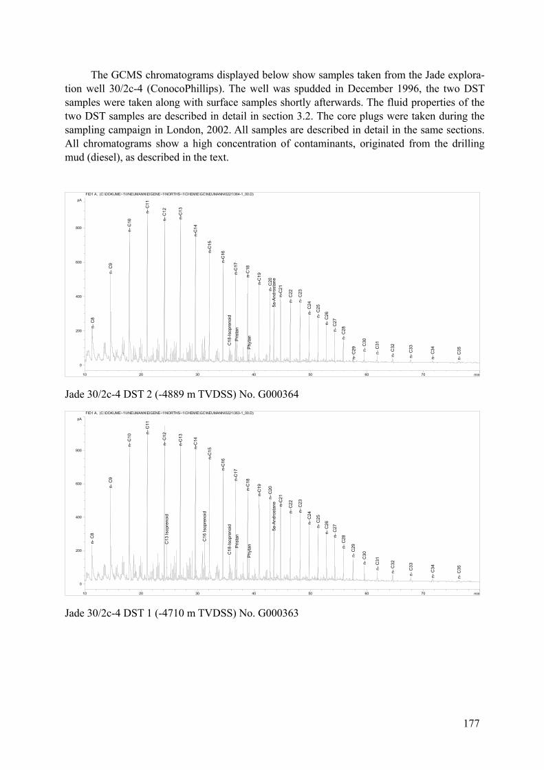
The GCMS chromatograms displayed below show samples taken from the Jade explora-tion well 30/2c-4 (ConocoPhillips). The well was spudded in December 1996, the two DST samples were taken along with surface samples shortly afterwards. The fluid properties of the two DST samples are described in detail in section 3.2. The core plugs were taken during the sampling campaign in London, 2002. All samples are described in detail in the same sections. All chromatograms show a high concentration of contaminants, originated from the drilling mud (diesel), as described in the text.

min10 20 30 40 50 60 70

pA

0

200

400

600

800

FID1 A, (C:\DOKUME~1\VNEUMANN\EIGENE~1\NORTHS~1\CHEMIE\GC\NEUMANN\0221\364-1_00.D)

n- C

8

n- C

9

n- C

10

n- C

11

n- C

12

n-C

13

n-C

14

n-C

15

n-C

16 C

18-Is

opre

noid

n-C

17

Pris

tan

n-C

18 P

hyta

n

n-C

19

n- C

20 5

a-A

ndro

stan

e n

-C21

n- C

22

n- C

23

n- C

24

n- C

25

n- C

26

n- C

27

n- C

28

n- C

29 n- C

30

n- C

31

n- C

32

n- C

33

n- C

34

n- C

35

Jade 30/2c-4 DST 2 (-4889 m TVDSS) No. G000364

min10 20 30 40 50 60 70

pA

0

200

400

600

800

FID1 A, (C:\DOKUME~1\VNEUMANN\EIGENE~1\NORTHS~1\CHEMIE\GC\NEUMANN\0221\363-1_00.D)

n- C

8

n- C

9

n- C

10

n- C

11

n- C

12 C

13 Is

opre

noid

n-C

13

n-C

14

C16

Isop

reno

id n

-C15

n-C

16 C

18-Is

opre

noid

n-C

17

Pris

tan

n-C

18 P

hyta

n

n-C

19

n- C

20 5

a-A

ndro

stan

e n

-C21

n- C

22

n- C

23

n- C

24

n- C

25

n- C

26

n- C

27

n- C

28

n- C

29

n- C

30

n- C

31

n- C

32

n- C

33

n- C

34

n- C

35

Jade 30/2c-4 DST 1 (-4710 m TVDSS) No. G000363

177

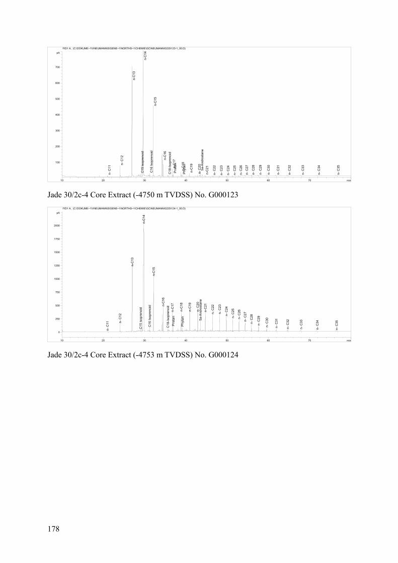
min10 20 30 40 50 60 70

pA

100

200

300

400

500

600

700

FID1 A, (C:\DOKUME~1\VNEUMANN\EIGENE~1\NORTHS~1\CHEMIE\GC\NEUMANN\0220\123-1_00.D)

n- C

11

n- C

12

n-C

13

C15

isop

reno

id n

-C14

C16

Isop

reno

id n

-C15

n-C

16 C

18-Is

opre

noid

n-C

17

Pris

tan

n-C

18 P

hyta

n

n-C

19

n- C

20 5

a-A

ndro

stan

e n

-C21

n- C

22

n- C

23

n- C

24

n- C

25

n- C

26

n- C

27

n- C

28

n- C

29

n- C

30

n- C

31

n- C

32

n- C

33

n- C

34

n- C

35

Jade 30/2c-4 Core Extract (-4750 m TVDSS) No. G000123

min10 20 30 40 50 60 70

pA

0

250

500

750

1000

1250

1500

1750

2000

FID1 A, (C:\DOKUME~1\VNEUMANN\EIGENE~1\NORTHS~1\CHEMIE\GC\NEUMANN\0220\124-1_00.D)

n- C

11 n- C

12

n-C

13

C15

isop

reno

id n

-C14

C16

Isop

reno

id n

-C15

n-C

16 C

18-Is

opre

noid

n-C

17

Pris

tan

n-C

18 P

hyta

n

n-C

19

n- C

20 5

a-A

ndro

stan

e n

-C21

n- C

22

n- C

23

n- C

24

n- C

25

n- C

26

n- C

27

n- C

28

n- C

29

n- C

30

n- C

31

n- C

32

n- C

33

n- C

34

n- C

35

Jade 30/2c-4 Core Extract (-4753 m TVDSS) No. G000124

178

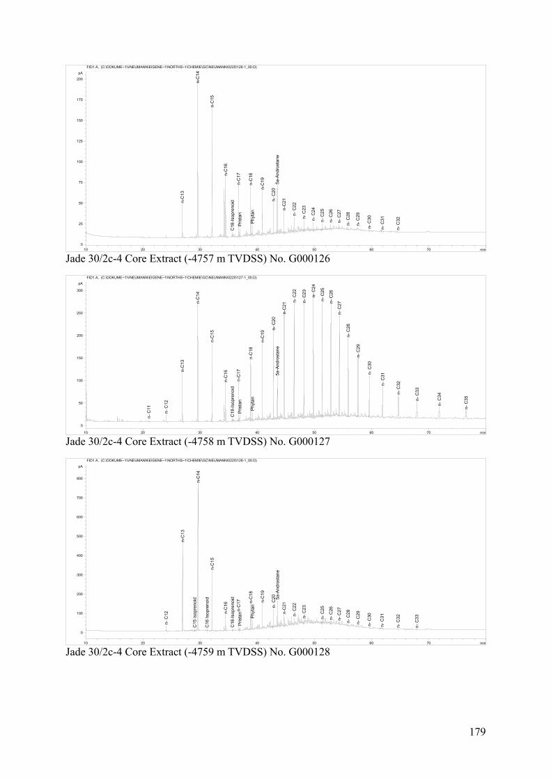
min10 20 30 40 50 60 70

pA

0

25

50

75

100

125

150

175

200

FID1 A, (C:\DOKUME~1\VNEUMANN\EIGENE~1\NORTHS~1\CHEMIE\GC\NEUMANN\0220\126-1_00.D)

n-C

13

n-C

14

n-C

15

n-C

16 C

18-Is

opre

noid

n-C

17

Pris

tan

n-C

18 P

hyta

n

n-C

19

n- C

20 5

a-A

ndro

stan

e n

-C21

n- C

22

n- C

23

n- C

24

n- C

25

n- C

26

n- C

27

n- C

28

n- C

29

n- C

30

n- C

31

n- C

32

Jade 30/2c-4 Core Extract (-4757 m TVDSS) No. G000126

min10 20 30 40 50 60 70

pA

0

50

100

150

200

250

300

FID1 A, (C:\DOKUME~1\VNEUMANN\EIGENE~1\NORTHS~1\CHEMIE\GC\NEUMANN\0220\127-1_00.D)

n- C

11

n- C

12

n-C

13

n-C

14

n-C

15

n-C

16 C

18-Is

opre

noid

n-C

17

Pris

tan

n-C

18 P

hyta

n

n-C

19

n- C

20 5

a-A

ndro

stan

e n

-C21 n

- C22

n- C

23

n- C

24

n- C

25

n- C

26

n- C

27

n- C

28

n- C

29

n- C

30

n- C

31

n- C

32

n- C

33

n- C

34

n- C

35

Jade 30/2c-4 Core Extract (-4758 m TVDSS) No. G000127

min10 20 30 40 50 60 70

pA

0

100

200

300

400

500

600

700

800

FID1 A, (C:\DOKUME~1\VNEUMANN\EIGENE~1\NORTHS~1\CHEMIE\GC\NEUMANN\0220\128-1_00.D)

n- C

12

n-C

13

C15

isop

reno

id n

-C14

C16

Isop

reno

id n

-C15

n-C

16 C

18-Is

opre

noid

n-C

17

Pris

tan

n-C

18 P

hyta

n

n-C

19

n- C

20 5a-

And

rost

ane

n-C

21

n- C

22

n- C

23

n- C

25

n- C

26

n- C

27

n- C

28

n- C

29

n- C

30

n- C

31

n- C

32

n- C

33

Jade 30/2c-4 Core Extract (-4759 m TVDSS) No. G000128

179

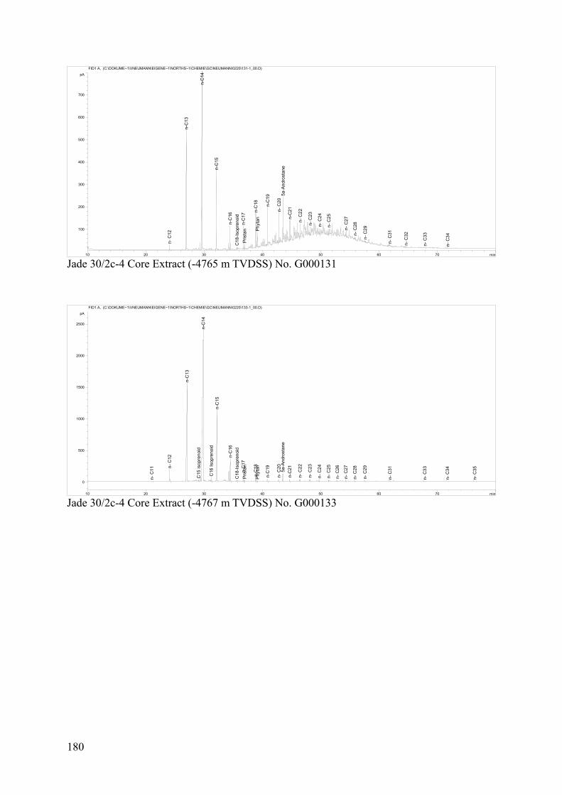
min10 20 30 40 50 60 70

pA

100

200

300

400

500

600

700

FID1 A, (C:\DOKUME~1\VNEUMANN\EIGENE~1\NORTHS~1\CHEMIE\GC\NEUMANN\0220\131-1_00.D)

n- C

12

n-C

13

n-C

14

n-C

15

n-C

16 C

18-Is

opre

noid

n-C

17

Pris

tan

n-C

18 P

hyta

n

n-C

19

n- C

20 5

a-A

ndro

stan

e n

-C21

n- C

22

n- C

23

n- C

24

n- C

25

n- C

27

n- C

28

n- C

29

n- C

31

n- C

32

n- C

33

n- C

34

Jade 30/2c-4 Core Extract (-4765 m TVDSS) No. G000131

min10 20 30 40 50 60 70

pA

0

500

1000

1500

2000

2500

FID1 A, (C:\DOKUME~1\VNEUMANN\EIGENE~1\NORTHS~1\CHEMIE\GC\NEUMANN\0220\133-1_00.D)

n- C

11 n- C

12

n-C

13

C15

isop

reno

id n

-C14

C16

Isop

reno

id n

-C15

n-C

16 C

18-Is

opre

noid

n-C

17

Pris

tan

n-C

18 P

hyta

n

n-C

19

n- C

20 5

a-A

ndro

stan

e n

-C21

n- C

22

n- C

23

n- C

24

n- C

25

n- C

26

n- C

27

n- C

28

n- C

29

n- C

31

n- C

33

n- C

34

n- C

35

Jade 30/2c-4 Core Extract (-4767 m TVDSS) No. G000133

180

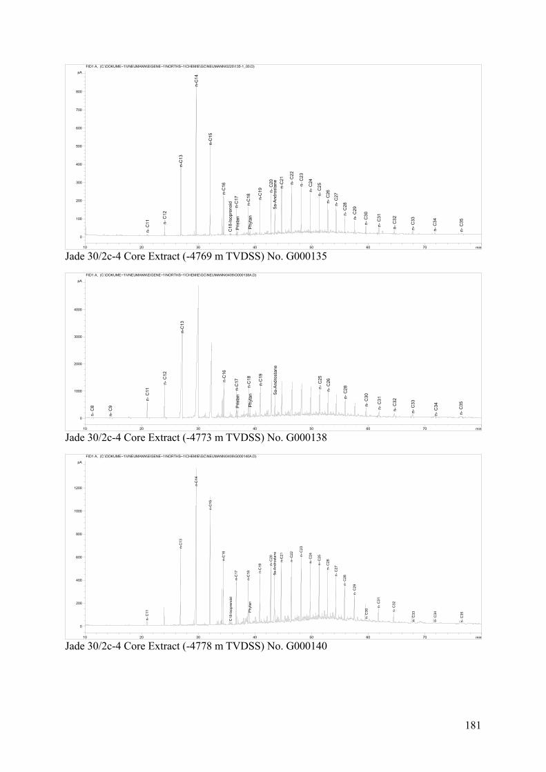
min10 20 30 40 50 60 70

pA

0

100

200

300

400

500

600

700

800

FID1 A, (C:\DOKUME~1\VNEUMANN\EIGENE~1\NORTHS~1\CHEMIE\GC\NEUMANN\0220\135-1_00.D)

n- C

11 n- C

12

n-C

13

n-C

14

n-C

15

n-C

16 C

18-Is

opre

noid

n-C

17

Pris

tan

n-C

18 P

hyta

n

n-C

19 n- C

20 5

a-A

ndro

stan

e n

-C21

n- C

22

n- C

23

n- C

24

n- C

25

n- C

26

n- C

27

n- C

28

n- C

29

n- C

30

n- C

31

n- C

32

n- C

33

n- C

34

n- C

35

Jade 30/2c-4 Core Extract (-4769 m TVDSS) No. G000135

min10 20 30 40 50 60 70

pA

0

1000

2000

3000

4000

FID1 A, (C:\DOKUME~1\VNEUMANN\EIGENE~1\NORTHS~1\CHEMIE\GC\NEUMANN\0409\G000138A.D)

n- C

8

n- C

9

n- C

11

n- C

12

n-C

13

n-C

16

n-C

17

Pris

tan

n-C

18 P

hyta

n

n-C

19

5a-

And

rost

ane

n- C

25

n- C

26

n- C

28

n- C

30

n- C

31

n- C

32

n- C

33

n- C

34

n- C

35

Jade 30/2c-4 Core Extract (-4773 m TVDSS) No. G000138

min10 20 30 40 50 60 70

pA

0

200

400

600

800

1000

1200

FID1 A, (C:\DOKUME~1\VNEUMANN\EIGENE~1\NORTHS~1\CHEMIE\GC\NEUMANN\0409\G000140A.D)

n- C

11

n-C

13

n-C

14

n-C

15

n-C

16

C18

-Isop

reno

id n

-C17

n-C

18 P

hyta

n

n-C

19 n- C

20 5

a-A

ndro

stan

e

n-C

21

n- C

22

n- C

23

n- C

24

n- C

25

n- C

26

n- C

27

n- C

28

n- C

29

n- C

30

n- C

31

n- C

32

n- C

33

n- C

34

n- C

35

Jade 30/2c-4 Core Extract (-4778 m TVDSS) No. G000140

181

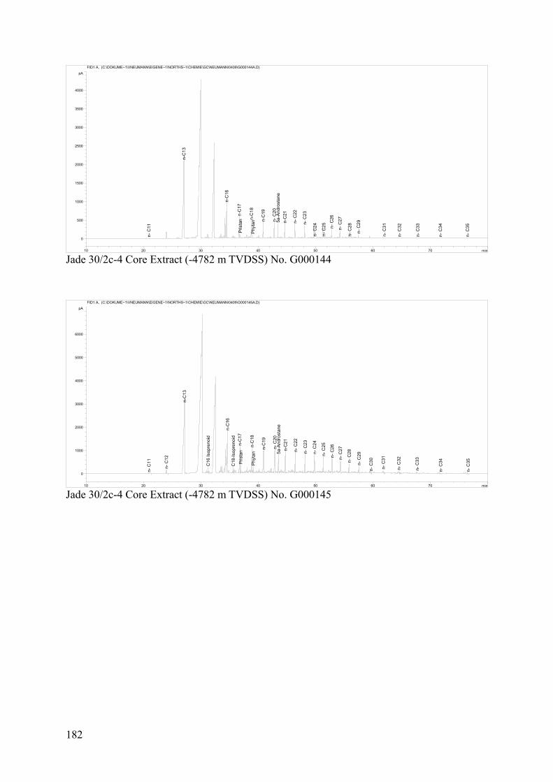
min10 20 30 40 50 60 70

pA

0

500

1000

1500

2000

2500

3000

3500

4000

FID1 A, (C:\DOKUME~1\VNEUMANN\EIGENE~1\NORTHS~1\CHEMIE\GC\NEUMANN\0409\G000144A.D)

n- C

11

n-C

13

n-C

16

n-C

17

Pris

tan n

-C18

Phy

tan n

-C19

n- C

20 5

a-A

ndro

stan

e n

-C21

n- C

22

n- C

23

n- C

24

n- C

25 n- C

26

n- C

27

n- C

28

n- C

29

n- C

31

n- C

32

n- C

33

n- C

34

n- C

35

Jade 30/2c-4 Core Extract (-4782 m TVDSS) No. G000144

min10 20 30 40 50 60 70

pA

0

1000

2000

3000

4000

5000

6000

FID1 A, (C:\DOKUME~1\VNEUMANN\EIGENE~1\NORTHS~1\CHEMIE\GC\NEUMANN\0409\G000145A.D)

n- C

11

n- C

12

n-C

13

C16

Isop

reno

id

n-C

16 C

18-Is

opre

noid

n-C

17

Pris

tan

n-C

18 P

hyta

n n-C

19

n- C

20 5

a-A

ndro

stan

e n

-C21

n- C

22

n- C

23

n- C

24

n- C

25

n- C

26

n- C

27

n- C

28

n- C

29

n- C

30

n- C

31

n- C

32

n- C

33

n- C

34

n- C

35

Jade 30/2c-4 Core Extract (-4782 m TVDSS) No. G000145

182

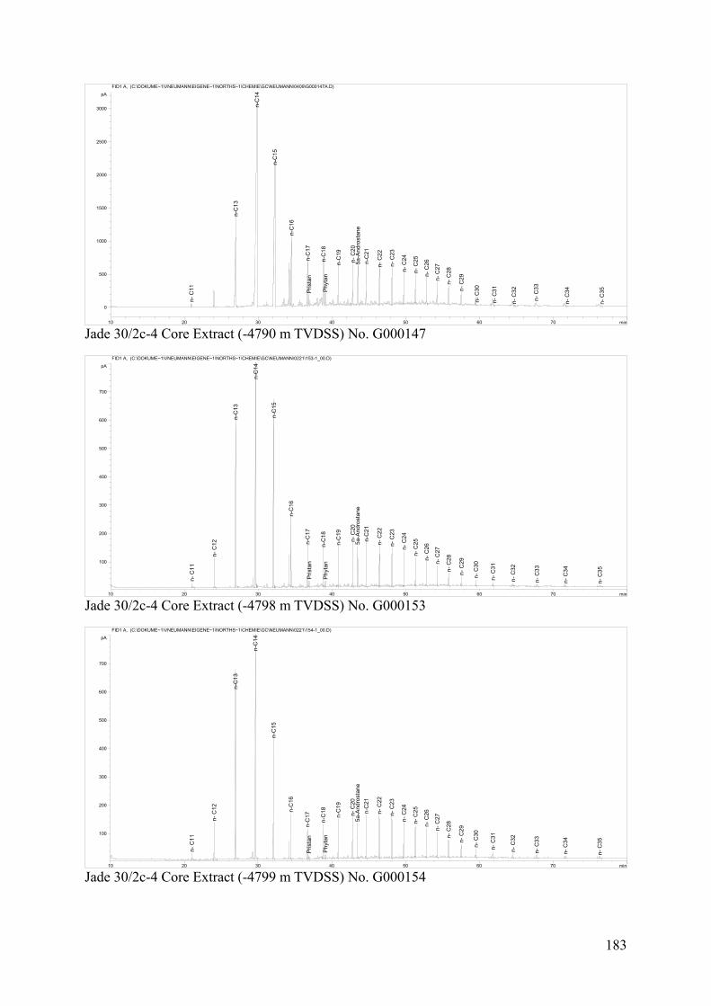
Jade 30/2c-4 Core Extract (-4790 m TVDSS) No. G000147 min10 20 30 40 50 60 70

pA

0

500

1000

1500

2000

2500

3000

FID1 A, (C:\DOKUME~1\VNEUMANN\EIGENE~1\NORTHS~1\CHEMIE\GC\NEUMANN\0409\G000147A.D)

n- C

11

n-C

13

n-C

14

n-C

15

n-C

16

n-C

17

Pris

tan

n-C

18 P

hyta

n

n-C

19

n- C

20 5

a-A

ndro

stan

e n

-C21

n- C

22

n- C

23

n- C

24

n- C

25

n- C

26

n- C

27

n- C

28

n- C

29

n- C

30

n- C

31

n- C

32

n- C

33

n- C

34

n- C

35min10 20 30 40 50 60 70

pA

100

200

300

400

500

600

700

FID1 A, (C:\DOKUME~1\VNEUMANN\EIGENE~1\NORTHS~1\CHEMIE\GC\NEUMANN\0221\153-1_00.D)

n- C

11

n- C

12

n-C

13

n-C

14

n-C

15

n-C

16

n-C

17

Pris

tan

n-C

18 P

hyta

n

n-C

19

n- C

20 5

a-A

ndro

stan

e n

-C21

n- C

22

n- C

23

n- C

24

n- C

25

n- C

26

n- C

27

n- C

28

n- C

29

n- C

30

n- C

31

n- C

32

n- C

33

n- C

34

n- C

35Jade 30/2c-4 Core Extract (-4798 m TVDSS) No. G000153

min10 20 30 40 50 60 70

pA

100

200

300

400

500

600

700

FID1 A, (C:\DOKUME~1\VNEUMANN\EIGENE~1\NORTHS~1\CHEMIE\GC\NEUMANN\0221\154-1_00.D)

n- C

11

n- C

12

n-C

13

n-C

14

n-C

15

n-C

16

n-C

17

Pris

tan

n-C

18 P

hyta

n

n-C

19

n- C

20 5

a-A

ndro

stan

e n

-C21

n- C

22

n- C

23

n- C

24

n- C

25

n- C

26

n- C

27

n- C

28

n- C

29

n- C

30

n- C

31

n- C

32

n- C

33

n- C

34

n- C

35

Jade 30/2c-4 Core Extract (-4799 m TVDSS) No. G000154

183

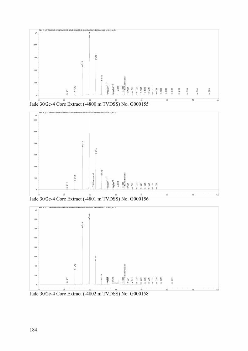
min10 20 30 40 50 60 70

pA

0

500

1000

1500

2000

FID1 A, (C:\DOKUME~1\VNEUMANN\EIGENE~1\NORTHS~1\CHEMIE\GC\NEUMANN\0221\155-1_00.D)

n- C

11

n- C

12

n-C

13

n-C

14

n-C

15

n-C

16

n-C

17

Pris

tan

n-C

18 P

hyta

n

n-C

19

n- C

20 5

a-A

ndro

stan

e n

-C21

n- C

22

n- C

23

n- C

24

n- C

25

n- C

26

n- C

27

n- C

28

n- C

29

n- C

30

n- C

31

n- C

32

n- C

33

n- C

34

n- C

35

Jade 30/2c-4 Core Extract (-4800 m TVDSS) No. G000155

min10 20 30 40 50 60 70

pA

0

500

1000

1500

2000

2500

3000

FID1 A, (C:\DOKUME~1\VNEUMANN\EIGENE~1\NORTHS~1\CHEMIE\GC\NEUMANN\0221\156-1_00.D)

n- C

11

n- C

12

n-C

13

C16

Isop

reno

id n

-C15

n-C

16

n-C

17

Pris

tan

n-C

18 P

hyta

n

n-C

19

n- C

20 5

a-A

ndro

stan

e n

-C21

n- C

22

n- C

23

n- C

24

n- C

25

n- C

26

n- C

27

n- C

28

Jade 30/2c-4 Core Extract (-4801 m TVDSS) No. G000156

min10 20 30 40 50 60 70

pA

0

200

400

600

800

1000

1200

1400

FID1 A, (C:\DOKUME~1\VNEUMANN\EIGENE~1\NORTHS~1\CHEMIE\GC\NEUMANN\0221\158-1_00.D)

n- C

11

n- C

12

n-C

13

n-C

14

n-C

15

n-C

16

n-C

17

Pris

tan

n-C

18

n- C

20 5a-

And

rost

ane

n-C

21

n- C

22

n- C

23

n- C

24

n- C

25

n- C

26

n- C

27

n- C

28

n- C

29

n- C

31

Jade 30/2c-4 Core Extract (-4802 m TVDSS) No. G000158

184

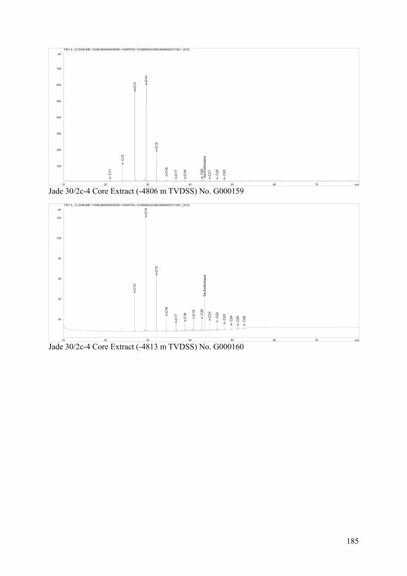
min10 20 30 40 50 60 70

pA

100

200

300

400

500

600

700

FID1 A, (C:\DOKUME~1\VNEUMANN\EIGENE~1\NORTHS~1\CHEMIE\GC\NEUMANN\0221\159-1_00.D)

n- C

11

n- C

12

n-C

13 n-C

14

n-C

15

n-C

16

n-C

17

n-C

18

n- C

20 5

a-A

ndro

stan

e n

-C21

n- C

22

n- C

23

Jade 30/2c-4 Core Extract (-4806 m TVDSS) No. G000159

min10 20 30 40 50 60 70

pA

20

40

60

80

100

120

FID1 A, (C:\DOKUME~1\VNEUMANN\EIGENE~1\NORTHS~1\CHEMIE\GC\NEUMANN\0221\160-1_00.D)

n-C

13

n-C

14

n-C

15

n-C

16

n-C

17

n-C

18

n-C

19

n- C

20 5

a-A

ndro

stan

e n

-C21

n- C

22

n- C

23

n- C

24

n- C

25

n- C

26

Jade 30/2c-4 Core Extract (-4813 m TVDSS) No. G000160

185

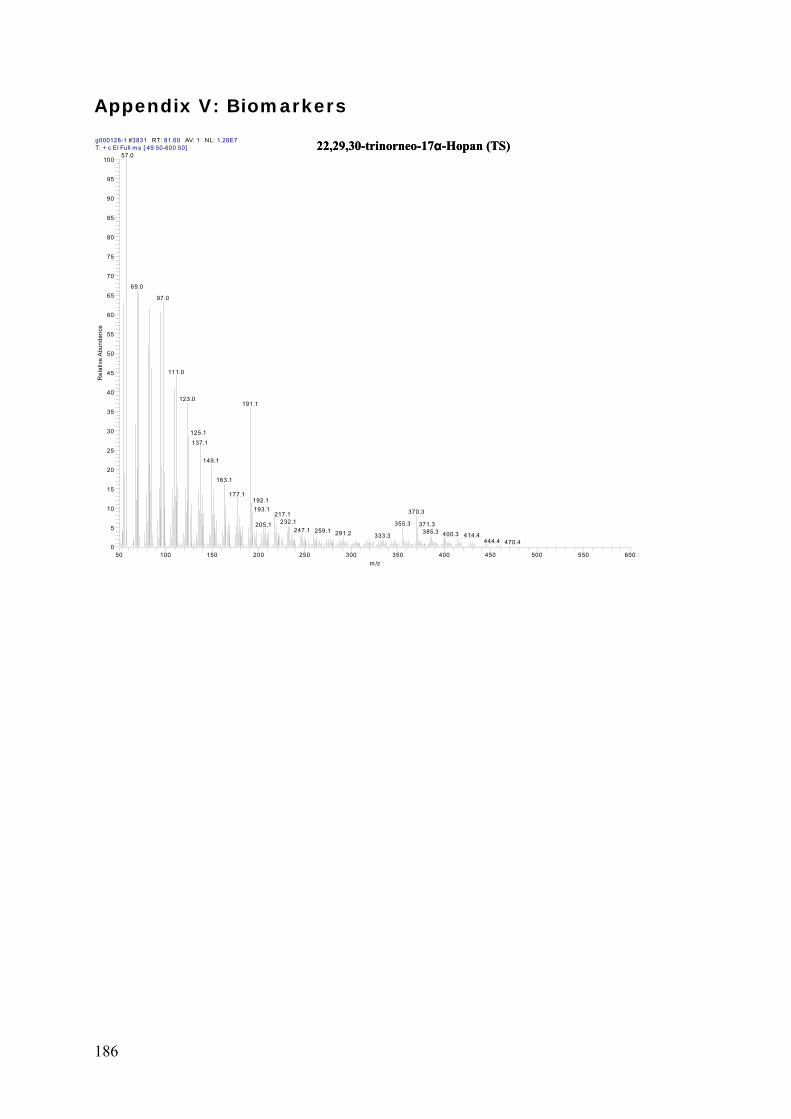
Appendix V: Biomarkers

22,29,30-trinorneo-17α-Hopan (TS)22,29,30-trinorneo-17α-Hopan (TS)g000128-1 #3831 RT: 81.60 AV: 1 NL: 1.28E7T: + c EI Full m s [ 49.50-600.50]

50 100 150 200 250 300 350 400 450 500 550 600m /z

0

5

10

15

20

25

30

35

40

45

50

55

60

65

70

75

80

85

90

95

100

Rel

ativ

e A

bund

ance

57.0

69.0

97.0

111.0

123.0191.1

125.1

137.1

149.1

163.1

177.1192.1193.1 370.3217.1

232.1 355.3 371.3205.1247.1 259.1 385.3291.2 400.3 414.4333.3

444.4 470.4

186

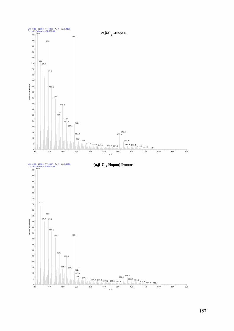
g000128-1 #3880 RT: 82.65 AV: 1 NL: 9.18E6T: + c EI Full m s [ 49.50-600.50]

50 100 150 200 250 300 350 400 450 500 550 600m /z

0

5

10

15

20

25

30

35

40

45

50

55

60

65

70

75

80

85

90

95

100

Rel

ativ

e A

bund

ance

57.0

191.1

95.0

69.081.0

97.0

109.0

111.0

149.1

125.1137.1

151.1163.1

192.1

177.1

370.3193.1 355.3

205.1217.1 371.3

233.1 259.1 385.3275.2 399.3319.3 331.3 414.4 444.4 460.4

α,β-C27-Hopanα,β-C27-Hopan

g000128-1 #3900 RT: 83.07 AV: 1 NL: 9.41E6T: + c EI Full m s [ 49.50-600.50]

50 100 150 200 250 300 350 400 450 500 550 600m /z

0

5

10

15

20

25

30

35

40

45

50

55

60

65

70

75

80

85

90

95

100

Rel

ativ

e A

bund

ance

57.0

71.0

95.0

81.0 97.0

109.0

191.1111.0

137.1

163.1

151.1 177.1192.1

193.1384.3205.1 369.3217.1 385.3261.2 275.2 414.3291.2 319.3 345.3 428.4 458.4 486.4

(α,β-C28-Hopan) Isomer(α,β-C28-Hopan) Isomer

187

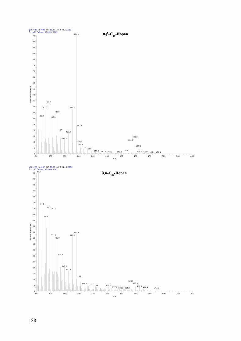
g000128-1 #4008 RT: 85.37 AV: 1 NL: 2.02E7T: + c EI Full m s [ 49.50-600.50]

50 100 150 200 250 300 350 400 450 500 550 600m /z

0

5

10

15

20

25

30

35

40

45

50

55

60

65

70

75

80

85

90

95

100

Rel

ativ

e Ab

unda

nce

191.1

95.0

81.0 177.1

123.0

69.0109.0

192.1

137.1163.1

398.3149.1

383.3193.1204.1

399.3217.1 231.1

369.3259.1 287.2 414.3 428.4301.2 343.2 456.4 472.4

α,β-C29-Hopanα,β-C29-Hopan

g000128-1 #4062 RT: 86.52 AV: 1 NL: 2.89E6T: + c EI Full m s [ 49.50-600.50]

50 100 150 200 250 300 350 400 450 500 550 600m /z

0

5

10

15

20

25

30

35

40

45

50

55

60

65

70

75

80

85

90

95

100

Rel

ativ

e A

bund

ance

57.0

71.0

95.0 97.0

83.0

191.1111.0 177.1

123.0

125.1

149.1

163.1

193.1

383.3398.3217.1 233.1 303.2259.1 413.3319.3 428.4343.3 361.3 474.4

β,α-C29-Hopanβ,α-C29-Hopan

188

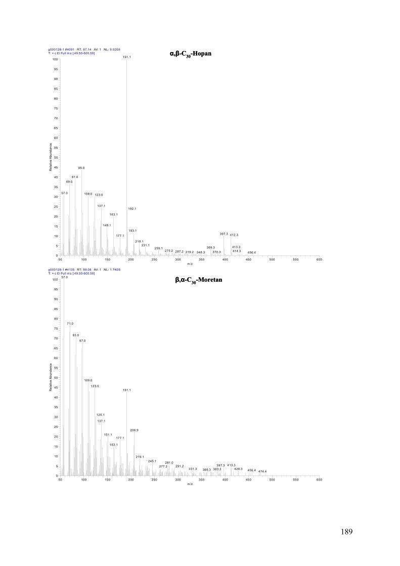
g000128-1 #4091 RT: 87.14 AV: 1 NL: 9.02E6T: + c EI Full m s [ 49.50-600.50]

50 100 150 200 250 300 350 400 450 500 550 600m /z

0

5

10

15

20

25

30

35

40

45

50

55

60

65

70

75

80

85

90

95

100

Rel

ativ

e A

bund

ance

191.1

95.0

81.069.0

57.0 109.0 123.0

137.1192.1

163.1

149.1

193.1397.3 412.3177.1

218.1231.1 413.3369.3259.1

275.2 414.3287.2 319.2 370.3348.3 456.4

α,β-C30-Hopanα,β-C30-Hopan

g000128-1 #4135 RT: 88.08 AV: 1 NL: 1.74E6T: + c EI Full m s [ 49.50-600.50]

50 100 150 200 250 300 350 400 450 500 550 600m /z

0

5

10

15

20

25

30

35

40

45

50

55

60

65

70

75

80

85

90

95

100

Rel

ativ

e A

bund

ance

57.0

71.0

83.0

97.0

109.0

123.0191.1

125.1

137.1

206.9151.1

177.1

163.1

219.1245.1 281.0

413.3397.3291.2277.2428.3331.3 383.3369.3 456.4 474.4

β,α-C30-Moretanβ,α-C30-Moretan

189

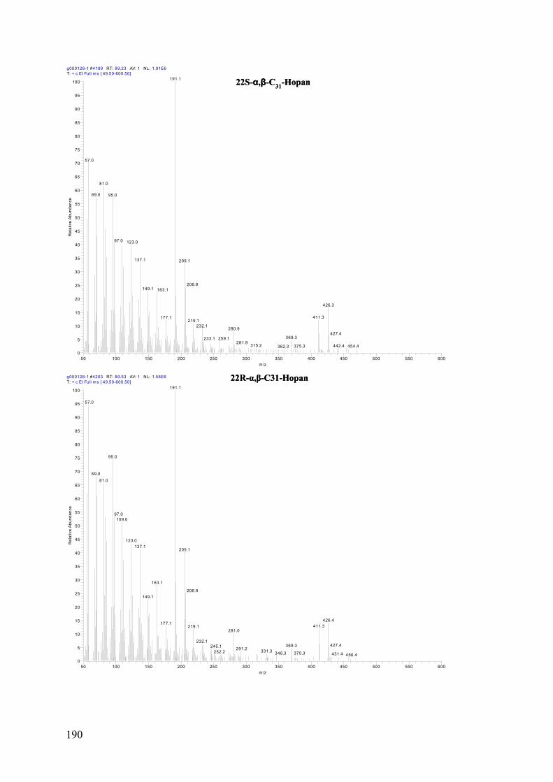
g000128-1 #4189 RT: 89.23 AV: 1 NL: 1.91E6T: + c EI Full m s [ 49.50-600.50]

50 100 150 200 250 300 350 400 450 500 550 600m /z

0

5

10

15

20

25

30

35

40

45

50

55

60

65

70

75

80

85

90

95

100

Rel

ativ

e A

bund

ance

191.1

57.0

81.0

69.0 95.0

97.0 123.0

137.1 205.1

206.9149.1 163.1

426.3

411.3177.1219.1

232.1280.9

427.4369.3233.1 259.1

281.9315.2 442.4375.3 454.4362.3

22S-α,β-C31-Hopan22S-α,β-C31-Hopan

g000128-1 #4203 RT: 89.53 AV: 1 NL: 1.58E6T: + c EI Full m s [ 49.50-600.50]

50 100 150 200 250 300 350 400 450 500 550 600m /z

0

5

10

15

20

25

30

35

40

45

50

55

60

65

70

75

80

85

90

95

100

Rel

ativ

e A

bund

ance

191.1

57.0

95.0

69.081.0

97.0109.0

123.0137.1

205.1

163.1

206.9149.1

426.4177.1

411.3219.1281.0

232.1427.4369.3245.1 291.2 331.3252.2 346.3 370.3 431.4 456.4

22R-α,β-C31-Hopan22R-α,β-C31-Hopan

190

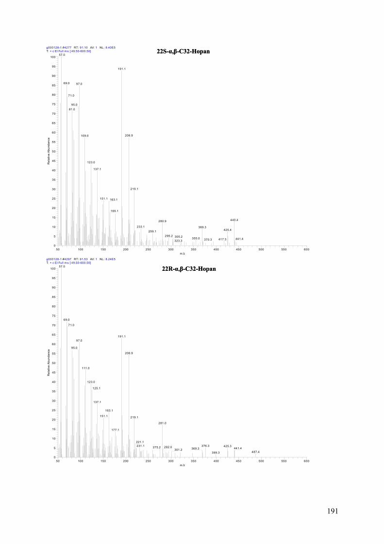
g000128-1 #4277 RT: 91.10 AV: 1 NL: 8.40E5T: + c EI Full m s [ 49.50-600.50]

50 100 150 200 250 300 350 400 450 500 550 600m /z

0

5

10

15

20

25

30

35

40

45

50

55

60

65

70

75

80

85

90

95

100

Rel

ativ

e A

bund

ance

57.0

191.1

69.0 97.0

71.0

95.081.0

206.9109.0

123.0

137.1

219.1

151.1 163.1

165.1

440.4280.9

233.1 369.3425.4259.1

295.2 305.2 355.0 441.4417.3370.3323.3

22S-α,β-C32-Hopan22S-α,β-C32-Hopan

g000128-1 #4297 RT: 91.53 AV: 1 NL: 8.24E5T: + c EI Full m s [ 49.50-600.50]

50 100 150 200 250 300 350 400 450 500 550 600m /z

0

5

10

15

20

25

30

35

40

45

50

55

60

65

70

75

80

85

90

95

100

Rel

ativ

e A

bund

ance

57.0

69.0

71.0

191.197.0

95.0

206.9

111.0

123.0

125.1

137.1

163.1

151.1 219.1

281.0

177.1

221.1376.3231.1 425.3282.0275.2 441.4369.3301.2

487.4399.3

22R-α,β-C32-Hopan22R-α,β-C32-Hopan

191

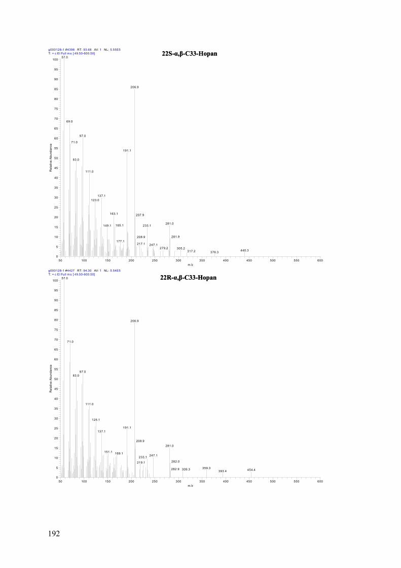
g000128-1 #4398 RT: 93.68 AV: 1 NL: 5.55E5T: + c EI Full m s [ 49.50-600.50]

50 100 150 200 250 300 350 400 450 500 550 600m /z

0

5

10

15

20

25

30

35

40

45

50

55

60

65

70

75

80

85

90

95

100

Rel

ativ

e A

bund

ance

57.0

206.9

69.0

97.0

71.0

191.1

83.0

111.0

137.1123.0

163.1 207.9

281.0165.1 233.1149.1

281.9208.9177.1

217.1 247.1279.2 305.2

440.3317.2 376.3

22S-α,β-C33-Hopan22S-α,β-C33-Hopan

g000128-1 #4427 RT: 94.30 AV: 1 NL: 5.54E5T: + c EI Full m s [ 49.50-600.50]

50 100 150 200 250 300 350 400 450 500 550 600m /z

0

5

10

15

20

25

30

35

40

45

50

55

60

65

70

75

80

85

90

95

100

Rel

ativ

e A

bund

ance

57.0

206.9

71.0

97.083.0

111.0

125.1

191.1137.1

208.9281.0

151.1 169.1247.1233.1

282.0219.1

359.3282.9 309.3 454.4393.4

22R-α,β-C33-Hopan22R-α,β-C33-Hopan

192