Numerical inversion of the dynamic model of a single-cylinder diesel engine

COMMUNICATIONS IN NUMERICAL METHODS IN ENGINEERINGCommun. Numer. Meth. Engng 2000; 16:505–517

Numerical inversion of the dynamic modelof a single-cylinder diesel engine

Yahya H. Zweiri, James F. Whidborne ∗ and Lakmal D. Seneviratne

Department of Mechanical Engineering; King’s College London; Strand; London WC2R 2LS; U.K.

SUMMARY

This paper presents a numerical technique to invert the dynamic model of a single-cylinder diesel engine. Themethod is employed to estimate the parameters of an engine from the data of crankshaft angular velocity,indicated torque, dynamometer angular velocity and applied load. The numerical inversion is performedduring both the transient and steady-state responses of the dynamic model. The method is developed with theaim of giving the designer information about the engine parameters which achieve a required performancecharacteristic (crankshaft velocity, indicated torque and applied load) and for tuning the parameters which playan important role in dynamic modelling. The model is implemented in MATLAB=SIMULINK, and simulationresults are presented. The simulation predictions of the engine and dynamometer parameters are compared withphysical values, and they are in excellent agreement. Further, a comparison between the measured crankshaftvelocity with simulated engine velocity calculated from the inverted parameters is presented, showing verygood agreement. Copyright ? 2000 John Wiley & Sons, Ltd.

KEY WORDS: diesel engine; dynamic modelling; numerical inversion; Newton–Raphson method; transientresponse; parameter tuning

1. INTRODUCTION

Inversion of an engine dynamic model has been established as an e�ective tool for studyingengine performance and contributing to design evaluation and new developments. Previous e�ortsin the area of inverting a dynamic engine model can be found in References [1–3]. The mainaim of these works is to use the engine dynamic model to describe the relationship between thecombustion pressure and engine angular velocity. This allows engine torque and cylinder pressureto be estimated from a measurement of crankshaft angular velocity which is more easily measuredthan cylinder pressure. The work of Zhang and Rizzoni [2] concentrates on the discrete frequenciescorresponding to the periodic rotation of the crankshaft; so it is only necessary to compute theengine dynamic model at the discrete frequencies, thus decreasing the computational time.

∗Correspondence to: J. F. Whidborne, Department of Mechanical Engineering, King’s College London, Strand, LondonWC2R 2LS, U.K.

Contract=grant sponsor: Mu’tah University, Hashemite Kingdom of Jordan

Received 23 April 1999Copyright ? 2000 John Wiley & Sons, Ltd. Accepted 12 January 2000

https://www.researchgate.net/publication/3153349_Estimate_of_indicated_torque_from_crankshaft_speed_fluctuations_A_model_for_the_dynamics_of_the_IC_engine?el=1_x_8&enrichId=rgreq-c60b759d-dace-461c-ae1c-6415158f02c1&enrichSource=Y292ZXJQYWdlOzIzNzA5OTQzMTtBUzoxMDY3NDU3MTYyODEzNDRAMTQwMjQ2MTU3MDE3Mg==

506 Y. H. ZWEIRI, J. F. WHIDBORNE AND L. D. SENEVIRATNE

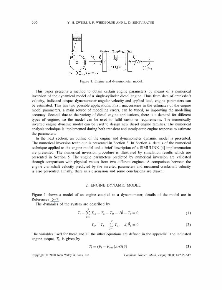
Figure 1. Engine and dynamometer model.

This paper presents a method to obtain certain engine parameters by means of a numericalinversion of the dynamical model of a single-cylinder diesel engine. Thus from data of crankshaftvelocity, indicated torque, dynamometer angular velocity and applied load, engine parameters canbe estimated. This has two possible applications. First, inaccuracies in the estimates of the enginemodel parameters, a main source of modelling errors, can be tuned, so improving the modellingaccuracy. Second, due to the variety of diesel engine applications, there is a demand for di�erenttypes of engines, so the model can be used to ful�l customer requirements. The numericallyinverted engine dynamic model can be used to design new diesel engine families. The numericalanalysis technique is implemented during both transient and steady-state engine response to estimatethe parameters.In the next section, an outline of the engine and dynamometer dynamic model is presented.

The numerical inversion technique is presented in Section 3. In Section 4, details of the numericaltechnique applied to the engine model and a brief description of a SIMULINK [4] implementationare presented. The numerical inversion procedure is illustrated by simulation results which arepresented in Section 5. The engine parameters predicted by numerical inversion are validatedthrough comparison with physical values from two di�erent engines. A comparison between theengine crankshaft velocity predicted by the inverted parameters and measured crankshaft velocityis also presented. Finally, there is a discussion and some conclusions are drawn.

2. ENGINE DYNAMIC MODEL

Figure 1 shows a model of an engine coupled to a dynamometer; details of the model are inReferences [5–7].The dynamics of the system are described by

Ti −5∑k=1Tfk − TS − TD − J ��− Tr = 0 (1)

TD + TS −N∑j=1TLj − J1 ��1 = 0 (2)

The variables used for these and all the other equations are de�ned in the appendix. The indicatedengine torque, Ti, is given by

Ti = (Pi − Patm)ArG(�) (3)

Copyright ? 2000 John Wiley & Sons, Ltd. Commun. Numer. Meth. Engng 2000; 16:505–517

https://www.researchgate.net/publication/3782006_Mathematical_transient_model_for_the_dynamics_of_a_single-cylinder_diesel_engine?el=1_x_8&enrichId=rgreq-c60b759d-dace-461c-ae1c-6415158f02c1&enrichSource=Y292ZXJQYWdlOzIzNzA5OTQzMTtBUzoxMDY3NDU3MTYyODEzNDRAMTQwMjQ2MTU3MDE3Mg==

https://www.researchgate.net/publication/237089214_Dynamic_simulation_of_a_single-cylinder_Diesel_engine_including_dynamometer_modelling_and_friction?el=1_x_8&enrichId=rgreq-c60b759d-dace-461c-ae1c-6415158f02c1&enrichSource=Y292ZXJQYWdlOzIzNzA5OTQzMTtBUzoxMDY3NDU3MTYyODEzNDRAMTQwMjQ2MTU3MDE3Mg==

https://www.researchgate.net/publication/237099431_Numerical_inversion_of_the_dynamic_model_of_a_single-cylinder_Diesel_engine?el=1_x_8&enrichId=rgreq-c60b759d-dace-461c-ae1c-6415158f02c1&enrichSource=Y292ZXJQYWdlOzIzNzA5OTQzMTtBUzoxMDY3NDU3MTYyODEzNDRAMTQwMjQ2MTU3MDE3Mg==

DYNAMIC MODELLING OF DIESEL ENGINE 507

where

G(�) = sin �+

√1− ��

cos � (4)

and

� = 1−(�+ r sin(�− �)

L

)2(5)

The piston displacement is given by

y =√(r + L)2 − �2 − [L cos � + r cos(�− �)] (6)

where

� = sin−1�

r + Land � = sin−1

�+ r sin(�− �)L

(7)

The friction torque terms,∑5

k=1 Tfk , are described as non-linear functions, which include pistonassembly friction, Tf 1 = f(r; �; �̇; �; Pi; h; B; d), bearing friction torque, Tf 2 = f(r; �; �̇; Db; Pi); valvetrain friction torque, Tf 3 = f(r; �̇; Div; niv; d), pumping losses torque, Tf 4 = f(�̇; Div; niv; nc; Vd);and pumps losses torque, Tf 5 = f(�̇; D; �; �; Vd). Details can be found in References [5; 6].The reciprocating torque, Tr , is produced due to the motion of the piston assembly and the small

end of the connecting rod and is given by

Tr = MrG(�) �y = MrG(�)[G1(�)�̇2+ G2(�) ��] (8)

where

G1(�) = r

[cos(�− �)

[1 +

(r=L) cos(�− �)�3=2

]−

√1− ��

sin(�− �)]

(9)

G2(�) = r

[sin(�− �) +

√1− ��

cos(�− �)]

(10)

and �y is the acceleration of the reciprocating components.The torsional sti�ness torque, TS , and damping torque, TD, which measure the sti�ness and the

damping in the coupling between the engine and the dynamometer respectively, are given by

TS = S(�− �1) (11)

and

TD = D(�̇− �̇1) (12)

Equations (1)–(12) lead to a set of non-linear di�erential equations which, given the indicatedpressure and the engine constant parameters, can be used to predict the motion of the engine andthe dynamometer. The dynamic model is implemented using MATLAB=SIMULINK [4; 8].



3. NUMERICAL INVERSION TECHNIQUE

Let there be n unknown system parameters in the vector p ∈ Rn×1. The dynamic equations(1)–(12), can be expressed as a function of p,

f(p) = 0 (13)

Thus given the measured data, engine angular velocity, indicated torque, dynamometer angularvelocity and dynamometer load, Equation (13) provides a single equation in the n unknown ele-ments of p. However, to �nd p, n independent equations are required. These equations are generatedby evaluating f, at discrete time intervals, t1; t2; : : : ; tn. In order to numerically invert the enginedynamic model, the system equations are expressed as functions of an engine parameters vectorp ∈ Rn×1.The engine dynamic equations (1)–(12), can now be expressed by n non-linear equations:

f1(p1; p2; : : : ; pn; t1) = 0

f2(p1; p2; : : : ; pn; t2) = 0

......

fn(p1; p2; : : : ; pn; tn) = 0

This system of n non-linear equations in n unknowns can alternatively be represented by de�ninga vector F ∈ Rn×1:

F(p1; p2; : : : ; pn) = (f1(p1; p2; : : : ; pn); f2(p1; p2; : : : ; pn); : : : ; fn(p1; p2; : : : ; pn))T = 0

(14)

Equation (14) can be written as

F(p) = 0: (15)

Let p0 be an initial estimate of p known to be in the vicinity of the actual solution of F(p).F(p) can now be expanded in a Taylor series about this point:

f1(p1; p2; : : : ; pn) = f01 +@f1@p1

∣∣∣∣0(p1 − p01) + @f1

@p2

∣∣∣∣0(p2 − p02) + · · ·

f2(p1; p2; : : : ; pn) = f02 +@f2@p1

∣∣∣∣0(p1 − p01) + @f2

@p2

∣∣∣∣0(p2 − p02) + · · ·

......

fn(p1; p2; : : : ; pn) = f0n +@fn@p1

∣∣∣∣0(p1 − p01) + @fn

@p2

∣∣∣∣0(p2 − p02) + · · ·

The zero subscript indicates that the functions and all partial derivatives are evaluated at p0. Bysetting F(p) = 0 in (16) gives n equations in the n unknowns p1; p2; : : : ; pn. These equations can



be solved using a generalized Newton–Raphson method:

p1p2...pn

≈

p01p02...p0n

−

@f1@p1

@f1@p2

: : :@f1@pn

@f2@p1

@f2@p2

: : :@f2@pn

......

......

@fn@p1

@fn@p2

: : :@fn@pn

−1∣∣∣∣∣∣∣∣∣∣∣∣∣∣∣∣∣∣0

f01f02...f0n

(16)

The Newton–Raphson method [9] gives rapid convergence, the accuracy approximately doublingwith each iteration [10].

4. IMPLEMENTATION OF THE NUMERICAL INVERSION TECHNIQUE

4.1. Parameter inversion technique

The numerical inversion technique is implemented for two di�erent engine operating modes, tran-sient and steady state. The transient response is used to estimate three parameters, that is p =(J;M; J1)T. Six parameters are estimated for the steady-state response, that is p = (S; D; d; r; L; Div)T.The discrete time intervals t1; t2; : : : ; tn, are uniformly spaced over a cycle for the steady-state

response, although the accuracy is not a�ected by the selection of the time intervals. But for thetransient response, since the engine speed is variable during this mode, the data must be sampledat the same angular position in each cycle. Thus the time interval is non-uniform for the transientresponse.For the transient response, the initial estimates need to be within about 60 per cent of their

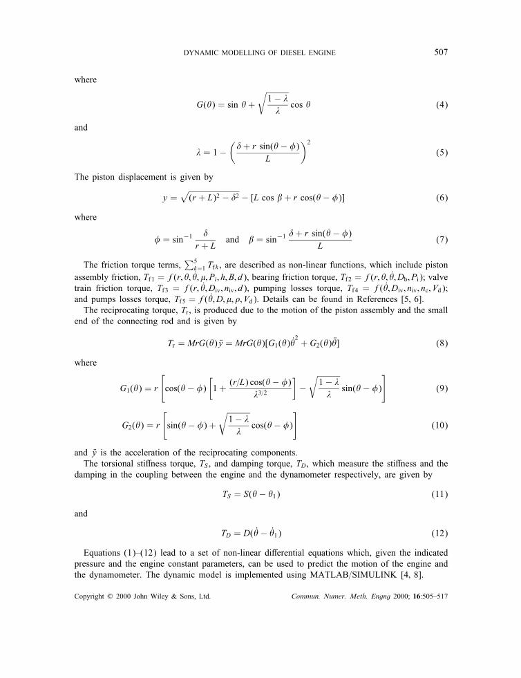
actual values for the method to correctly converge, however, for the steady-state estimation theparameters always converged.Prior to sampling, the angular velocity and indicated torque data were averaged over each

cycle to reduce noise and the uctuations resulting from higher-order crankshaft vibrations and thereactive forces from the engine and dynamometer mountings, as shown in Figure 2.

4.2. MATLAB/SIMULINK implementation

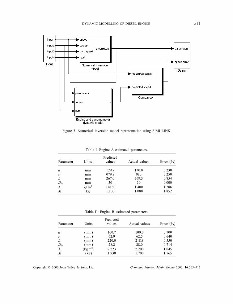
The technique is implemented using MATLAB=SIMULINK. Figure 3 shows the structure of theSIMULINK model for the numerical inversion technique. The input block contains the measureddata, crankshaft velocity, indicated torque, dynamometer velocity and applied load. The outputblock contains the engine and dynamometer parameters and speed comparison diagrams. The nu-merical inversion block consists of the non-linear Newton–Raphson method estimate the systemparameters from the input data. The engine dynamic model block contains the model described inSection 2. A comparison of the estimated crankshaft velocity with the measured data is performedin the comparison block.A variable-step Runge–Kutta (4,5) method was used for the simulation. The program was exe-

cuted on a 400 MHz Pentium II PC. and took about 7 min to complete.



Figure 2. Engine speed: (a) before averaging (—–) and after averaging (- - -), indicated torque: (b) beforeaveraging (—–) and after averaging (- - -).

5. RESULTS AND MODEL VALIDATION

In order to validate the numerical inversion model, both transient and steady-state estimations wereperformed for two single-cylinder diesel engines, labelled A and B, using the same dynamometer.The measured data for engine A are taken from Reference [11].Initial estimates of J are made from a knowledge of the moments of inertia of the large

ywheels, crankshafts, rotating parts of connecting rods and main gears. The predicted values areslightly less than the estimates obtained from the numerical inversion model as shown in Tables Iand II. These discrepancies arise from the fact that the system is time variant and the measureddata is averaged at each cycle during the transient response, and the inertia of auxiliary systems(alternator, water pump, fuel pump, oil pump, and camshaft) contribute to the engine moment ofinertia. The equivalent masses, M , are approximately computed by considering the mass of pistons,rings, wrist pins, and the small end of connecting rods. These values are slightly less than theestimates obtained from the model as shown in Tables I and II. These discrepancies arise due tothe averaging of data at each cycle and due to the small amount of mass near the small end alsocontributing to the reciprocating motion. The other values, Div, d, r, and L are very close to theestimated values.



Figure 3. Numerical inversion model representation using SIMULINK.

Table I. Engine A estimated parameters.

PredictedParameter Units values Actual values Error (%)

d mm 129:7 130:0 0:230r mm 079:8 080 0:250L mm 267:0 269:3 0:854Div mm 30 30 0:000J kgm2 1:4180 1:400 1:286M kg 1:100 1:080 1:852

Table II. Engine B estimated parameters.


d (mm) 100.7 100.0 0.700r (mm) 62.9 62.5 0.640L (mm) 220.0 218.8 0.550Div (mm) 28.2 28.0 0.714J (kgm2) 2.223 2.200 1.045M (kg) 1.730 1.700 1.765



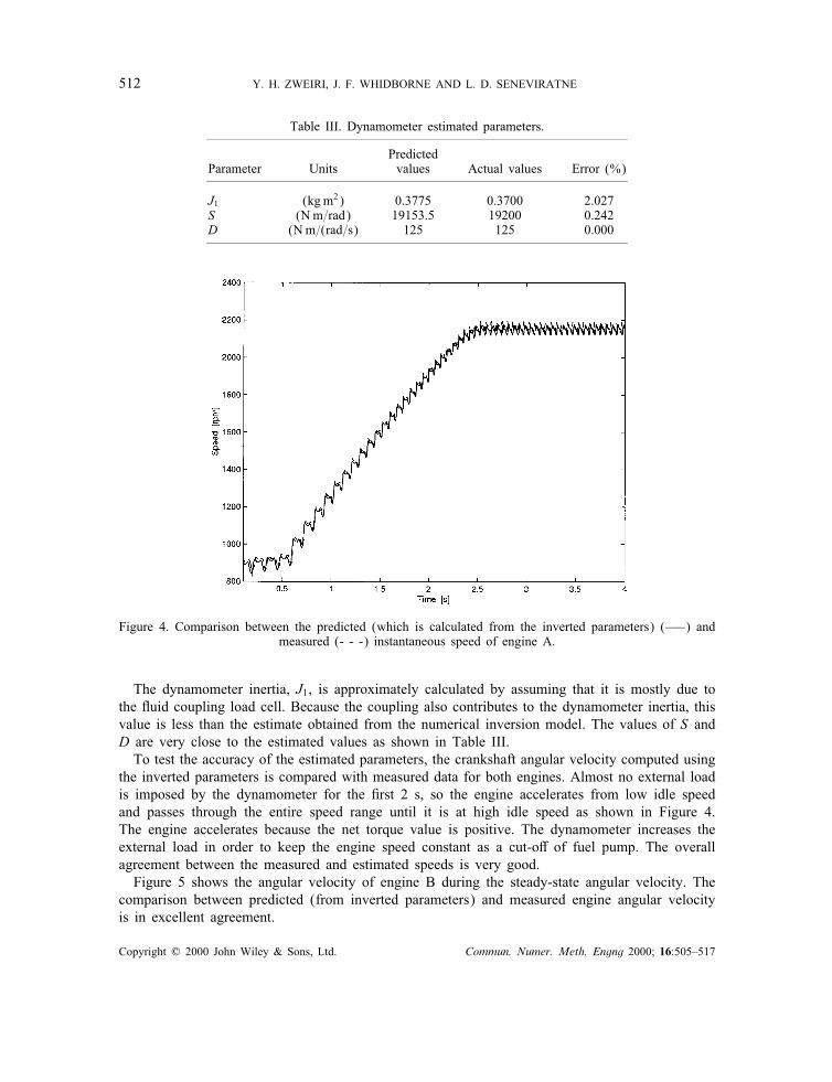
Table III. Dynamometer estimated parameters.


J1 (kgm2) 0.3775 0.3700 2.027S (Nm=rad) 19153.5 19200 0.242D (Nm=(rad=s) 125 125 0.000

Figure 4. Comparison between the predicted (which is calculated from the inverted parameters) (—–) andmeasured (- - -) instantaneous speed of engine A.

The dynamometer inertia, J1, is approximately calculated by assuming that it is mostly due tothe uid coupling load cell. Because the coupling also contributes to the dynamometer inertia, thisvalue is less than the estimate obtained from the numerical inversion model. The values of S andD are very close to the estimated values as shown in Table III.To test the accuracy of the estimated parameters, the crankshaft angular velocity computed using

the inverted parameters is compared with measured data for both engines. Almost no external loadis imposed by the dynamometer for the �rst 2 s, so the engine accelerates from low idle speedand passes through the entire speed range until it is at high idle speed as shown in Figure 4.The engine accelerates because the net torque value is positive. The dynamometer increases theexternal load in order to keep the engine speed constant as a cut-o� of fuel pump. The overallagreement between the measured and estimated speeds is very good.Figure 5 shows the angular velocity of engine B during the steady-state angular velocity. The

comparison between predicted (from inverted parameters) and measured engine angular velocityis in excellent agreement.



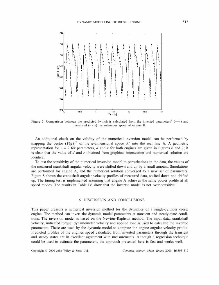
Figure 5. Comparison between the predicted (which is calculated from the inverted parameters) (—–) andmeasured (- - -) instantaneous speed of engine B.

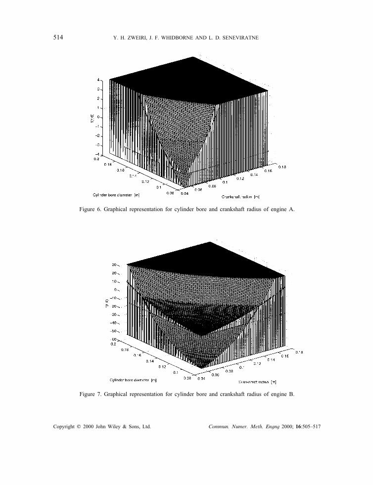
An additional check on the validity of the numerical inversion model can be performed bymapping the vector (F(p))T of the n-dimensional space Rn into the real line R. A geometricrepresentation for n = 2 for parameters, d and r for both engines are given in Figures 6 and 7; itis clear that the value of d and r obtained from graphical intersection and numerical solution areidentical.To test the sensitivity of the numerical inversion model to perturbations in the data, the values of

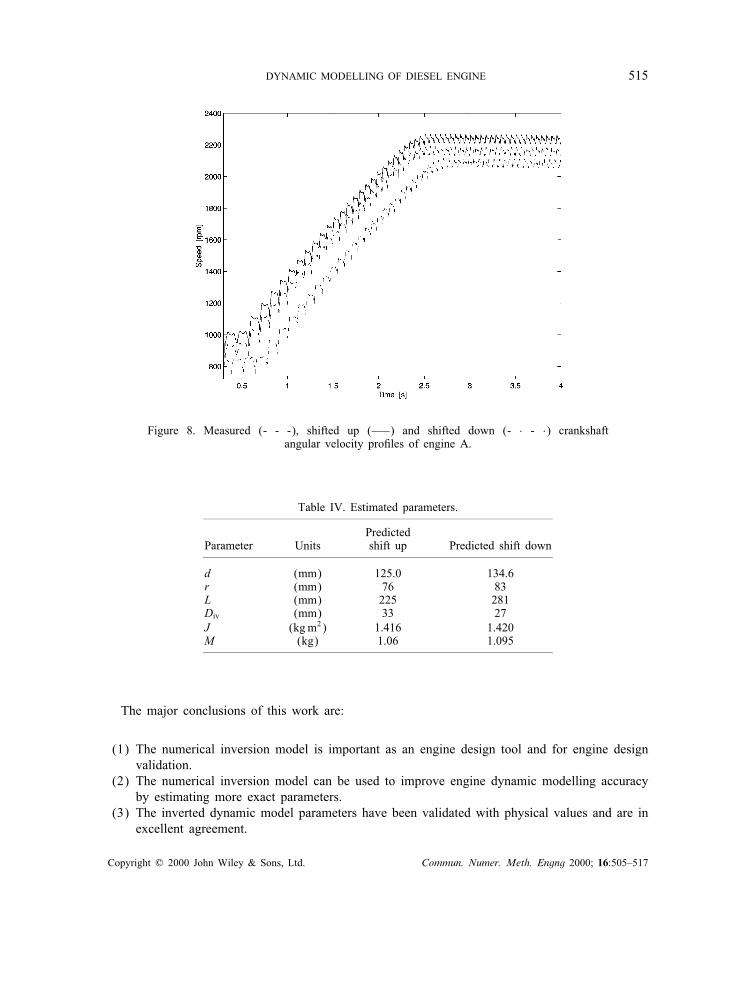
the measured crankshaft angular velocity were shifted down and up by a small amount. Simulationsare performed for engine A, and the numerical solution converged to a new set of parameters.Figure 8 shows the crankshaft angular velocity pro�les of measured data, shifted down and shiftedup. The tuning test is implemented assuming that engine A achieves the same power pro�le at allspeed modes. The results in Table IV show that the inverted model is not over sensitive.

6. DISCUSSION AND CONCLUSIONS

This paper presents a numerical inversion method for the dynamics of a single-cylinder dieselengine. The method can invert the dynamic model parameters at transient and steady-state condi-tions. The inversion model is based on the Newton–Raphson method. The input data, crankshaftvelocity, indicated torque, dynamometer velocity and applied load is used to calculate the invertedparameters. These are used by the dynamic model to compute the engine angular velocity pro�le.Predicted pro�les of the engines speed calculated from inverted parameters through the transientand steady states are in excellent agreement with measurements. Although a regression techniquecould be used to estimate the parameters, the approach presented here is fast and works well.



Figure 6. Graphical representation for cylinder bore and crankshaft radius of engine A.

Figure 7. Graphical representation for cylinder bore and crankshaft radius of engine B.



Figure 8. Measured (- - -), shifted up (—–) and shifted down (- · - ·) crankshaftangular velocity pro�les of engine A.

Table IV. Estimated parameters.

PredictedParameter Units shift up Predicted shift down

d (mm) 125.0 134.6r (mm) 76 83L (mm) 225 281Div (mm) 33 27J (kgm2) 1.416 1.420M (kg) 1.06 1.095

The major conclusions of this work are:

(1) The numerical inversion model is important as an engine design tool and for engine designvalidation.

(2) The numerical inversion model can be used to improve engine dynamic modelling accuracyby estimating more exact parameters.

(3) The inverted dynamic model parameters have been validated with physical values and are inexcellent agreement.



APPENDIX: NOMENCLATURE

A piston area (m2)B the width of the ring in the direction of motion (slider width) (m)d cylinder bore diameter (m)D damping coe�cient (Nm=(rad=s))Db bearing diameter (m)Div intake valve diameter (m)

G, G1, and G2(�) geometric functionsh total oil �lm thickness (m)j subscript to identify each load at di�erent timeJ moment of inertia of crankshaft, ywheel, main gear and rotating part of

connecting rod (kgm2)J1 moment of inertia of dynamometer rotating parts (kgm2)k subscript to identify each friction torque of the engineL connecting rod length (m)M piston, rings, pin and small end of connecting rod mass (kg)nc number of cylindersniv number of intake valvesPatm atmospheric pressure(101 kPa)Pi indicated pressure (Pa)p model parameters vectorp0 model starting points parameters vectorr crankshaft radius (m)S sti�ness (Nm=rad)TD damping torque (Nm)Tf 1 piston-ring assembly friction torque (Nm)Tf 2 crankshaft bearing friction torque (Nm)Tf 3 valve train friction torque (Nm)Tf 4 pumping losses torque (Nm)Tf 5 pumps friction torque (Nm)Ti indicated torque (Nm)TLj engine load torque (Nm)Tr reciprocating inertia torque (Nm)TS torsional sti�ness torque (Nm)Vd displacement volume (m3)y piston displacement (m)� connecting rod angle (rad)� piston pin o�set (m)� crankshaft angular position (rad)�1 dynamometer angular position (rad)� the dynamic viscosity of the oil (N s=m2)� oil density (kg=m3)� connecting rod angle when piston is at top dead centre (rad)



ACKNOWLEDGEMENTS

The authors would like to thank Mr D. Wareing of Perkins Technology for his support, and Dr D. N. Fenner,Dr K. C. Lee and Dr K. A. Althoefer for their suggestions and help. This research is partly �nanced bythe Hashemite Kingdom of Jordan and Mu’tah University. The �rst author is most grateful to ProfessorE. Dahiyat for his encouragement and help.

REFERENCES

1. Rizzoni G. Estimate of indicated torque from crankshaft speed uctuations: a model for the dynamics of the IC engine.IEEE Transactions on Vehicular Technology 1989; 38(3):168–179.

2. Zhang Y, Rizzoni G. An on-line indicated torque estimator for IC engine diagnosis and control. ASME Journal ofAdvanced Automotive Technology 1993; 52:147–162.

3. Citron S, O’Higgins J, Chen L. Cylinder by cylinder engine pressure torque waveform determination utilizing crankshaftspeed uctuation. SAE paper No. 890486, 1989.

4. The MathWorks, Inc., MA, U.S.A. SIMULINK: A Program for Simulating Dynamic Systems, 1997.5. Zweiri YH, Whidborne JF, Seneviratne LD. A mathematical transient model for the dynamics of a single cylinderdiesel engine. Proceedings of the Simulation ’98, York, U.K., September 1998; 145–151.

6. Zweiri YH, Whidborne JF, Seneviratne LD. Dynamic simulation of a single-cylinder diesel engine includingdynamometer modelling and friction. Proceedings of the Institution of Mechanical Engineers Part D 1999; 213:391–402.

7. Zweiri YH, Whidborne JF, Seneviratne LD. Numerical inversion of the dynamic model of a single-cylinder dieselengine. Proceedings of Spring Engine Techonology Conference ASME ICE, Vol. 3, Columbus, U.S.A., 1999;139–149.

8. The MathWorks, Inc., MA, U.S.A. MATLAB: Reference Guide, 1997.9. Burden RL, Faires JD. Numerical Analysis. Brooks Cole: Paci�c Grove, 1997.10. Mathews JH. Numerical Methods for Mathematics, Science, and Engineering. Prentice-Hall: Englewood Cli�s,

NJ, 1992.11. Filipi ZS, Assanis DN. A non-linear, transient, single-cylinder diesel engine simulation for predictions of instantaneous

engine speed and torque. Proceedings of the Tech. Conference ASME ICE, vol. 1, Colorado, U.S.A., 1997; 61–70.












Numerical inversion of the dynamic model of a single-cylinder diesel engine

Documents

Transcript of Numerical inversion of the dynamic model of a single-cylinder diesel engine