Ann Oper Res (2006) 141: 67–83

DOI 10.1007/s10479-006-5294-8

Numerical analysis of (s, S) inventory systems withrepeated attempts

J.R. Artalejo · A. Krishnamoorthy ·M.J. Lopez-Herrero

C© Springer Science + Business Media, Inc. 2006

Abstract This paper deals with a continuous review (s, S) inventory system where arriving

demands finding the system out of stock, leave the service area and repeat their request after

some random time. This assumption introduces a natural alternative to classical approaches

based either on lost demand models or on backlogged models. The stochastic model formu-

lation is based on a bidimensional Markov process which is numerically solved to investigate

the essential operating characteristics of the system. An optimal design problem is also

considered.

Keywords Inventory models . Numerical methods of truncation . Repeated attempts .

Stationary distribution

AMS subject classification: 90B05 . 90B22

1. Introduction

The stochastic modeling and performance analysis of inventory models form an integral part

of the Operations Research and the Applied Probability literature (see Tijms (1994) and the

references therein). An important feature in inventory models is to specify what happens

J.R. ArtalejoDepartment of Statistics and Operations Research, Faculty of Mathematics, Complutense University ofMadrid, Madrid 28040, Spaine-mail: jesus artalejo@mat.ucm.es

A. KrishnamoorthyDepartment of Mathematics, Cochin University of Science and Technology, Cochin 682022, Indiae-mail: ak@cusat.ac.in

M.J. Lopez-HerreroSchool of Statistics, Complutense University of Madrid, Madrid 28040, Spaine-mail: lherrero@estad.ucm.es

Springer

68 Ann Oper Res (2006) 141: 67–83

when a demand finds a system out of stock, i.e., the inventory on hand is zero. Two classical

situations are considered in the literature:

(i) Lost-sales case. The blocked demands arriving when the stock level is zero are

lost.

(ii) Backlog case. The demand arriving while the inventory system is out of stock are back-

logged and are satisfied as soon as an appropriate replenishment occurs.

The inventory model investigated in this paper offers a third option to the blocked de-

mands consisting in to leave temporally the service area but the demand is repeated after

some random time until it finds a positive stock level. This description arises frequently

in daily life situations when a customer visiting a retail store or a warehouse finds that

the stock of any salable good is empty and he must wait for some time before to try his

luck again. The consideration of the repeated request as an element of the inventory model

can be justified in practice due to a variety of reasons: (i) In contrast to the lost-sales and

backlog cases, the organization does not incur any expenditure towards lost sales nor for

holding unsatisfied demands; (ii) the blocked demands would prefer the repeated order op-

tion to avoid the payment of a deposit made as guarantee for the backlogged unit; (iii) the

physical characteristics of the warehouse can disable the option of backlogging the blocked

demands.

There exists a rich variety of different inventory models depending on the combination of

different assumptions. Some specific and common assumptions are as follows: continuous

versus periodic review of the inventory, individual versus batch demands, different replen-

ishment policies (fixed or random size, order-up-to level S), constant or random lead times,

etc. In this paper we will investigate an inventory model based on a policy of type (s, S)

operating under the presence of a non-homogeneous flow of repeated attempts due to the

existence of previous blocked demands.

Since the pioneering work of Arrow, Harris, and Marschak (1951) the continuous review

(s, S) inventory model has attracted a great deal of attention. Many authors have proposed

inventory systems based on (s, S) policies. Our model is close to the continuous system

proposed by Srinivasan (1979) (lost-sales case) and Sahin (1983) (backlog case). As far

as we know no work has been done in inventory models that take into account the retrial

phenomenon occurring after blocking of those demands finding a system out of stock, so

the joint consideration of inventories and retrials is the main goal of this paper. However,

the study of queueing systems with repeated calls is a topic that has received a considerable

attention in the last decades (Artalejo and Falin, 2002; Falin and Templeton, 1997). Our

approach to investigate numerically the stationary distribution of the inventory model under

consideration is inspired in the generalized truncated techniques developed in the context of

multiserver Markovian retrial queues (Artalejo and Pozo, 2002).

The stochastic modeling of complex inventory systems yields frequently to the use of two-

dimensional (or indeed multi-dimensional) inventory structures. This is a common feature

of the inventory system with repeated orders investigated in this paper and other models like

the model with item returns studied by Fleischmann, Kuik, and Dekker (2002) and Yuan and

Cheung (1998) and the production-inventory model subject to failures considered by Wang,

Cao, and Liu (2002).

The rest of the paper is organized as follows. Section 2 introduces the inventory model

and some notation. The main results relating to the algorithmic solution of the stationary

probabilities are presented in Section 3. Some particular cases are discussed in Section 4 and

finally, Section 5 is dedicated to numerical results and optimization.

Springer

Ann Oper Res (2006) 141: 67–83 69

2. Formulation of the model

We consider a single-item, continuous review (s, S) inventory model. Primary demands are

assumed to follow a Poisson process with rate λ > 0. Let us assume that the inventory level

at time t = 0 equals the maximum inventory level S. As soon as the stock level drops down

to s, a replenishment order for S − s units is placed, i.e., s is the reorder level. The maximum

level S is assumed to be greater than 2s. It should be pointed out that no more than one

replenishment order can be outstanding at the same time. Thus, the assumption S > 2s is

essential and it avoids perpetual order placement. The lead times are independent, identically

distributed random variables following an exponential law of rate ν > 0. If the stock level

was to drop to level zero, a demand arriving and finding the system out of stock leaves

the service area (i.e., the retail shop, the warehouse, . . . ) temporally but it makes successive

repeated attempts until the repeated demand finds a positive inventory level and consequently

it can be satisfied. Between trials we say that a blocked demand is on the retrial group. A

demand at the retrial group generates a source of repeated attempts independently of the

rest of demands in the retrial group. Thus, the probability of a repeated attempt during the

interval (t, t + dt), given that j demands are in the retrial group at time t , is jμ + o(dt).We also assume that the inter-demand periods, lead times and retrial times are mutually

independent.

The system state at time t can be described by means of a bivariate process X ={(I (t), R(t)); t ≥ 0}, where I (t) is the inventory level and R(t) is the number of blocked

demands in the retrial group at time t. Under the above assumptions the process X is

a regular continuous time Markov chain with the lattice semi-strip E = {0, . . . , S} ×Z+ as state space. Figure 1 illustrates the transitions among the states for the case

(s, S) = (2, 6).

Fig. 1 Process X : State space and transitions

Springer

70 Ann Oper Res (2006) 141: 67–83

The infinitesimal transition rates of process X are as follows. For i = 0 and j ≥ 0, we

have

q(0, j),(m,n) =

⎧⎪⎪⎪⎨⎪⎪⎪⎩λ, if (m, n) = (0, j + 1),

ν, if (m, n) = (S − s, j),

−(λ + ν), if (m, n) = (0, j),

0, otherwise.

(2.1)

For 1 ≤ i ≤ s and j ≥ 0, we have

q(i, j),(m,n) =

⎧⎪⎪⎪⎪⎪⎪⎨⎪⎪⎪⎪⎪⎪⎩

λ, if (m, n) = (i − 1, j),

ν, if (m, n) = (i + S − s, j),

jμ, if (m, n) = (i − 1, j − 1),

−(λ + ν + jμ), if (m, n) = (i, j),

0, otherwise,

(2.2)

and for s + 1 ≤ i ≤ S and j ≥ 0:

q(i, j),(m,n) =

⎧⎪⎪⎪⎨⎪⎪⎪⎩λ, if (m, n) = (i − 1, j),

jμ, if (m, n) = (i − 1, j − 1),

−(λ + jμ), if (m, n) = (i, j),

0, otherwise.

(2.3)

In the next section we will prove that the process X is positive recurrent if and only if

λ < (S − s)ν. Under this condition the stationary probabilities Pi j = limt→∞ P{I (t) = i,R(t) = j} exist for all (i, j) ∈ E and are positive. It should be noted that our inventory

model governed by the infinitesimal generator Q can be viewed as an M/M/c retrial queue

in which departures occur only if the number of customers in the service facility is greater

than c′, 0 < c′ ≤ c, and customers are served in batches of constant size c′. This analogy

is useful to understand the complicated structure of process X. Even with the Markovian

assumption the problem exhibits considerable complexity due to the spatial heterogeneity

caused by the transitions associated with the repeated attempts (Artalejo and Pozo, 2002;

Falin and Templeton, 1997). Thus, as it occurs in retrial queues, we overcome the analytical

difficulties by formulating a generalized truncated process in which all the essential operating

characteristics are rooted. This is done in the next section.

3. Performance analysis

In this section we study the process X modeling the inventory system with repeated attempts

when it is operating under the stable regime. Hence, the first question to be investigated is

the condition of positive recurrence.

Theorem 3.1. The process X = {(I (t), R(t)); t ≥ 0} is positive recurrent if and only if λ <

(S − s)ν.Springer

Ann Oper Res (2006) 141: 67–83 71

Proof: Let {Xn ; n ≥ 0} be the embedded Markov chain at the transition epochs of the

process X . Let also q(i, j) be the rate of the exponential distribution that governs the length

of a sojourn time in state (i, j) ∈ E for the continuous process X . Note that q(i, j) ≥ λ > 0,

for all (i, j) ∈ E, so a sufficient condition for the positive recurrence of {Xn ; n ≥ 0} is also

sufficient for the positive recurrence of process X in continuous time.

For an irreducible and aperiodic discrete time Markov chain {Xn ; n ≥ 0} with state space

E, a sufficient condition for positive recurrence is the existence of a non-negative func-

tion f (s), s ∈ S, a positive number ε and a finite subset H ⊂ E such that the mean drift

γs = E[ f (Xn+1) |Xn = s ] − f (s) is finite for all i ∈ S and γs ≤ −ε for all s /∈ H (Foster’s

criterion). Let us consider f (i, j) = a(S − i) + j , where the constant a should be determined

later. Then, we obtain

γ(i, j) =

⎧⎪⎪⎪⎪⎪⎪⎨⎪⎪⎪⎪⎪⎪⎩

λ − a(S − s)ν

λ + ν, if i = 0, j ≥ 0,

a(λ − (S − s)ν) + (a − 1) jμ

λ + ν + jμ, if 1 ≤ i ≤ s, j ≥ 0,

aλ + (a − 1) jμ

λ + jμ, if s + 1 ≤ i ≤ S, j ≥ 0.

For 1 ≤ i ≤ S, we note that γ(i, j) → a − 1, as j → ∞. Now we can choose the constant

a belonging to the interval ( λ(S−s)ν

, 1) and ε = 12

min{1 − a, a(S−s)ν−λ

λ+ν}. Since γ(i, j) < −ε

for all (i, j) ∈ E except perhaps for a finite number, the sufficiency follows from Foster’s

criterion.

We now define the subset Ek = {(i, j) ∈ E |S − i + j ≤ k } , for each k ≥ 0. By equating

the flow rate in and out of the subset Ek, we have

λ = (S − s)νs∑

i=0

∞∑j=0

Pi j .

Under the normalization condition∑

(i, j)∈E Pi j = 1, the term on the right hand side of

the above formula is bounded by (S − s)ν, so we conclude the necessity. �

We now introduce a generalized truncated model which preserves the main features of

the original inventory model X and provides a tractable numerical approximate analysis of

the stationary probabilities {Pi j ; (i, j) ∈ E}. As far as the number of demands in the retrial

group increases the retrial rate tends to infinity. In the light of this fact, our truncated inventory

model is based on the following assumption: we assume that the retrial rate becomes infinity

when R(t) exceeds a certain threshold level M.

Let X M = {(I M (t), RM (t)); t ≥ 0

}be the Markov process denoting the system state in

the approximate model. Note that the process X M corresponds to an inventory model with

repeated attempts in which the retrial rate μ j , given that the number of demands in the retrial

group is j, is given by

μ j ={

jμ, if 0 ≤ j ≤ M,

∞, if j ≥ M + 1.

Springer

72 Ann Oper Res (2006) 141: 67–83

Fig. 2 Process X M : State space and transitions

The state space associated to process X M is E M = {1, . . . , S} × {0, . . . , M} ∪ {0} × Z+.

Its infinitesimal generator QM has the following elements:

(i) if 0 ≤ i ≤ S, 0 ≤ j ≤ M , then q M(i, j),(m,n) = q(i, j),(m,n),

(ii) if i = 0, j ≥ M + 1, then

q M(0, j),(m,n) =

⎧⎪⎪⎪⎪⎪⎪⎨⎪⎪⎪⎪⎪⎪⎩

λ, if (m, n) = (0, j + 1),

ν,if j < M + S − s and (m, n) = (S − s − j + M, M)

or if j ≥ M + S − s and (m, n) = (0, j − S + s),

−(λ + ν), if (m, n) = (i, j),

0, otherwise.

Figure 2 illustrates the transitions among states and is helpful to understand the dynamic

of the approximate model X M .

The positive recurrent condition of process X M is λ < (S − s)ν which will be assumed

in the sequel. The proof is similar to the one shown in Theorem 3.1 for the process X so the

Springer

Ann Oper Res (2006) 141: 67–83 73

details are now omitted. We only remark that the mean drifts γ M(0, j), for j ≥ M + S − s, of

process X M are given by

γ M(0, j) = λ − (S − s)ν

λ + ν, j ≥ M + S − s.

The stationary probabilities {P Mi j ; (i, j) ∈ E M } satisfy the system of Kolmogorov equa-

tions �pM QM = �0, where �pM is a vector containing the stationary probabilities P Mi j re-

arranged in lexicographical order. Let us introduce new variables {r Mi j ; (i, j) ∈ E M } de-

fined as r Mi j = P M

i j /P M0M , for (i, j) ∈ E M , which are useful for computing recursively the

stationary probabilities. Note that the relationship between P Mi j and the new unknowns

r Mi j is P M

i j = r Mi j (

∑(m,n)∈E M r M

mn)−1. We observe that the variables r Mi j satisfy the following

system of equations:

(λ + ν)r M0 j = (1 − δ j0)λr M

0, j−1 + λr M1 j + ( j + 1)μr M

1, j+1, 0 ≤ j ≤ M − 1, (3.1)

(λ + ν + jμ)r Mi j = λr M

i+1, j + ( j + 1)μr Mi+1, j+1, 1 ≤ i ≤ s, 0 ≤ j ≤ M − 1, (3.2)

(λ + jμ)r Mi j = λr M

i+1, j + ( j + 1)μr Mi+1, j+1, s + 1 ≤ i ≤ S − s − 1,

0 ≤ j ≤ M − 1, (3.3)

(λ + jμ)r Mi j = (1 − δi S)λr M

i+1, j + (1 − δi S)( j + 1)μr Mi+1, j+1 + νr M

i−S+s, j ,

S − s ≤ i ≤ S, 0 ≤ j ≤ M − 1, (3.4)

(λ + ν)r M0M = (1 − δM0)λr M

0,M−1 + λr M1M + νr M

0,M+S−s, (3.5)

(λ + ν + Mμ)r Mi M = λr M

i+1,M + νr M0,M+S−s−i , 1 ≤ i ≤ s, (3.6)

(λ + Mμ)r Mi M = λr M

i+1,M + νr M0,M+S−s−i , s + 1 ≤ i ≤ S − s − 1, (3.7)

(λ + Mμ)r Mi M = (1 − δi S)λr M

i+1,M + νr Mi−S+s,M , S − s ≤ i ≤ S, (3.8)

(λ + ν)r M0 j = λr M

0, j−1 + νr M0, j+S−s, j ≥ M + 1, (3.9)

where δi j denotes the Kronecker’s symbol

δi j ={

1, if i = j,

0, if i �= j.

To solve the system of equations (3.1)–(3.9), we first take generating functions in equation

(3.9). By denoting F(z) = ∑∞j=M+1 z jr M

0 j , we find that

F(z) = λzM+S−s+1r M0M − ν

∑M+S−sj=M+1 z jr M

0 j

(λ(1 − z) + ν)zS−s − ν. (3.10)

Springer

74 Ann Oper Res (2006) 141: 67–83

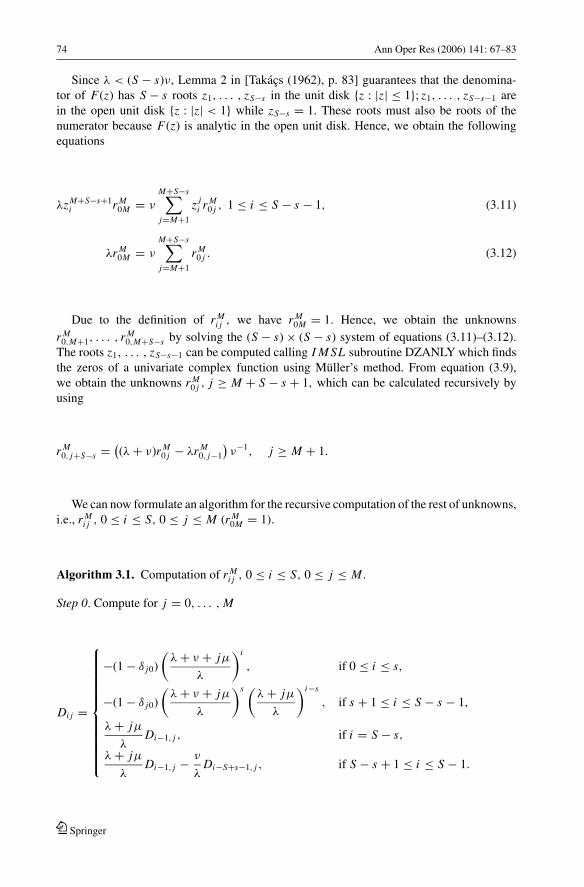
Since λ < (S − s)ν, Lemma 2 in [Takacs (1962), p. 83] guarantees that the denomina-

tor of F(z) has S − s roots z1, . . . , zS−s in the unit disk {z : |z| ≤ 1}; z1, . . . , zS−s−1 are

in the open unit disk {z : |z| < 1} while zS−s = 1. These roots must also be roots of the

numerator because F(z) is analytic in the open unit disk. Hence, we obtain the following

equations

λzM+S−s+1i r M

0M = ν

M+S−s∑j=M+1

z ji r M

0 j , 1 ≤ i ≤ S − s − 1, (3.11)

λr M0M = ν

M+S−s∑j=M+1

r M0 j . (3.12)

Due to the definition of r Mi j , we have r M

0M = 1. Hence, we obtain the unknowns

r M0,M+1, . . . , r M

0,M+S−s by solving the (S − s) × (S − s) system of equations (3.11)–(3.12).

The roots z1, . . . , zS−s−1 can be computed calling I M SL subroutine DZANLY which finds

the zeros of a univariate complex function using Muller’s method. From equation (3.9),

we obtain the unknowns r M0 j , j ≥ M + S − s + 1, which can be calculated recursively by

using

r M0, j+S−s = (

(λ + ν)r M0 j − λr M

0, j−1

)ν−1, j ≥ M + 1.

We can now formulate an algorithm for the recursive computation of the rest of unknowns,

i.e., r Mi j , 0 ≤ i ≤ S, 0 ≤ j ≤ M (r M

0M = 1).

Algorithm 3.1. Computation of r Mi j , 0 ≤ i ≤ S, 0 ≤ j ≤ M .

Step 0. Compute for j = 0, . . . , M

Di j =

⎧⎪⎪⎪⎪⎪⎪⎪⎪⎪⎪⎪⎨⎪⎪⎪⎪⎪⎪⎪⎪⎪⎪⎪⎩

−(1 − δ j0)

(λ + ν + jμ

λ

)i

, if 0 ≤ i ≤ s,

−(1 − δ j0)

(λ + ν + jμ

λ

)s (λ + jμ

λ

)i−s

, if s + 1 ≤ i ≤ S − s − 1,

λ + jμ

λDi−1, j , if i = S − s,

λ + jμ

λDi−1, j − ν

λDi−S+s−1, j , if S − s + 1 ≤ i ≤ S − 1.

Springer

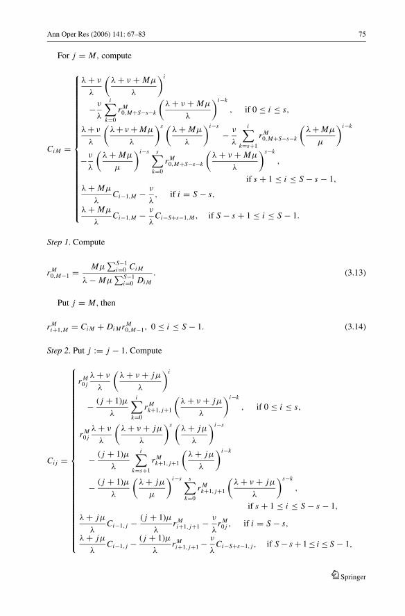
Ann Oper Res (2006) 141: 67–83 75

For j = M, compute

Ci M =

⎧⎪⎪⎪⎪⎪⎪⎪⎪⎪⎪⎪⎪⎪⎪⎪⎪⎪⎪⎪⎪⎪⎪⎨⎪⎪⎪⎪⎪⎪⎪⎪⎪⎪⎪⎪⎪⎪⎪⎪⎪⎪⎪⎪⎪⎪⎩

λ + ν

λ

(λ + ν + Mμ

λ

)i

−ν

λ

i∑k=0

r M0,M+S−s−k

(λ + ν + Mμ

λ

)i−k

, if 0 ≤ i ≤ s,

λ + ν

λ

(λ + ν + Mμ

λ

)s (λ + Mμ

λ

)i−s

− ν

λ

i∑k=s+1

r M0,M+S−s−k

(λ + Mμ

μ

)i−k

−ν

λ

(λ + Mμ

μ

)i−s s∑k=0

r M0,M+S−s−k

(λ + ν + Mμ

λ

)s−k

,

if s + 1 ≤ i ≤ S − s − 1,λ + Mμ

λCi−1,M − ν

λ, if i = S − s,

λ + Mμ

λCi−1,M − ν

λCi−S+s−1,M , if S − s + 1 ≤ i ≤ S − 1.

Step 1. Compute

r M0,M−1 = Mμ

∑S−1i=0 Ci M

λ − Mμ∑S−1

i=0 Di M

. (3.13)

Put j = M , then

r Mi+1,M = Ci M + Di Mr M

0,M−1, 0 ≤ i ≤ S − 1. (3.14)

Step 2. Put j := j − 1. Compute

Ci j =

⎧⎪⎪⎪⎪⎪⎪⎪⎪⎪⎪⎪⎪⎪⎪⎪⎪⎪⎪⎪⎪⎪⎪⎪⎪⎪⎪⎪⎪⎪⎨⎪⎪⎪⎪⎪⎪⎪⎪⎪⎪⎪⎪⎪⎪⎪⎪⎪⎪⎪⎪⎪⎪⎪⎪⎪⎪⎪⎪⎪⎩

r M0 j

λ + ν

λ

(λ + ν + jμ

λ

)i

− ( j + 1)μ

λ

i∑k=0

r Mk+1, j+1

(λ + ν + jμ

λ

)i−k

, if 0 ≤ i ≤ s,

r M0 j

λ + ν

λ

(λ + ν + jμ

λ

)s (λ + jμ

λ

)i−s

− ( j + 1)μ

λ

i∑k=s+1

r Mk+1, j+1

(λ + jμ

λ

)i−k

− ( j + 1)μ

λ

(λ + jμ

μ

)i−s s∑k=0

r Mk+1, j+1

(λ + ν + jμ

λ

)s−k

,

if s + 1 ≤ i ≤ S − s − 1,

λ + jμ

λCi−1, j − ( j + 1)μ

λr M

i+1, j+1 − ν

λr M

0 j , if i = S − s,

λ + jμ

λCi−1, j − ( j + 1)μ

λr M

i+1, j+1 − ν

λCi−S+s−1, j , if S − s + 1 ≤ i ≤ S − 1,

Springer

76 Ann Oper Res (2006) 141: 67–83

and

r M0, j−1 = jμ

∑S−1i=0 Ci j

λ − jμ∑S−1

i=0 Di j

. (3.15)

Calculate recursively

r Mi+1, j = Ci j + Di jr

M0, j−1, 0 ≤ i ≤ S − 1. (3.16)

Step 3. Repeat step 2 until j = 0.

Proof: The proof follows after some algebraic manipulations over the set of equations (3.1)–

(3.8). We now indicate only the main steps. First of all, we employ equations (3.5)–(3.7) to

express r Mi+1,M as a linear function of r M

i M , for 0 ≤ i ≤ S − s − 1. Then a backward recur-

sion allows us to get expression (3.14) for 0 ≤ i ≤ S − s − 1. An appeal to equation (3.8)

completes the scheme for S − s ≤ i ≤ S − 1. We neglect equation (3.8) for i = S and al-

ternatively we use the equation obtained by equating the flow rate into and out of the subset{(i, j) ∈ E | j ≤ M − 1 }:

λr M0,M−1 = Mμ

S∑i=1

r Mi M . (3.17)

By combining expressions (3.14) and (3.17) we easily find (3.13). Then, we decrease in

one unit the level of the retrial group and proceed with equations (3.1)–(3.4). By employing

parallel arguments we get formulas (3.15) and (3.16). Finally, when the algorithm reaches

the level j = 0 we observe that Di0 = 0, 0 ≤ i ≤ S − 1, so we can determine r M00 and then

r Mi0 , 1 ≤ i ≤ S. �

In Section 5 we will discuss the numerical analysis of the approximate inventory model

X M . In order to evaluate the efficiency of the generalized truncated model, we now intro-

duce another model based on a finite truncation. Both inventory models will be compared

numerically in Section 5.

We next consider a finite truncated inventory model which consist in replacing the infinite

state space E by another truncated finite space E K obtained by placing a finite limit Kon the retrial group capacity. Let X K = {

(I K (t), RK (t)); t ≥ 0}

be the process describing

the inventory state and the number of blocked demands in the retrial group at time t . The

process X K is a continuous time bivariate Markov chain with state space E K = {0, . . . , S} ×{0, . . . , K } . If we denote as λi j the arrival rate of primary demands when the system state

is (i, j), then the direct truncated inventory model X K corresponds to the case

λi j ={

λ, if (i, j) ∈ E K − {(0, K )} ,

0, if (i, j) = (0, K ),

i.e., the approximate model X K can be viewed as an inventory model with partial lost-sales

where primary demands finding a system out of stock and a fully occupance of the retrial

group must abandon the system.

Since X K is an aperiodic and irreducible Markov chain taking values on a finite state space,

we know that X K is positive recurrent for any choice of the system parameters λ > 0, ν > 0,

Springer

Ann Oper Res (2006) 141: 67–83 77

μ > 0 and K ∈ Z+. The stationary probabilities P Ki j = limt→∞ P{I K (t) = i, RK (t) = j},

(i, j) ∈ E K , can be recursively computed by modifying the scheme proposed for process

X M in Algorithm 3.1. Let us consider the unknowns r Ki j = P K

i j /P K0K which satisfy a system

formed by equations (3.1)–(3.4) and (3.8) (replacing the threshold M by K ) and the new

equations

νr K0K = (1 − δK 0)λr K

0,K−1 + λr K1K , (3.18)

(λ + ν + Kμ)r Ki K = λr K

i+1,K , 1 ≤ i ≤ s, (3.19)

(λ + Kμ)r Ki K = λr K

i+1,K , s + 1 ≤ i ≤ S − s − 1. (3.20)

From equations (3.18)–(3.20), we find that

r Ki+1,K = Ci K + Di K r K

0,K−1, 0 ≤ i ≤ S − s − 1,

where

Ci K =

⎧⎪⎪⎪⎨⎪⎪⎪⎩ν

λ

(λ + ν + Kμ

λ

)i

, for 0 ≤ i ≤ s,

ν

λ

(λ + ν + Kμ

λ

)s (λ + Kμ

λ

)i−s

, for s + 1 ≤ i ≤ S − s − 1,

Di K =

⎧⎪⎪⎪⎨⎪⎪⎪⎩−(1 − δK 0)

(λ + ν + Kμ

λ

)i

, for 0 ≤ i ≤ s,

−(1 − δK 0)

(λ + ν + Kμ

λ

)s (λ + Kμ

λ

)i−s

, for s + 1 ≤ i ≤ S − s − 1.

The rest of the recursive scheme for the computation of r Ki j follows the steps given in

Algorithm 3.1.

4. Special cases

As special cases of our inventory model with repeated attempts, we can derive some simple

systems where the demands finding upon arrival that the stock level is zero either abandon

the system or they are backlogged.

Let us consider the truncated model X K in the extreme case where K equals 0. The

following result provides explicit expressions for the stationary probabilities. These for-

mulas are supplemental to the work done in Srinivasan (1979) for the continuous re-

view (s, S) inventory model in the lost-sales case. The proof of Proposition 4.1 follows

the arguments leading to the recursive scheme proposed in Theorem 3.1. We first get

the unknowns r Ki j (case K = 0) and, in a second round, we obtain P K

i j . For ease of nota-

tion, we denote P0i j simply as Qi j .

Proposition 4.1. The stationary distribution of the continuous review inventory model withexponential lead times and losses of the blocked demands corresponds to the special case of

Springer

78 Ann Oper Res (2006) 141: 67–83

the model X K where K = 0. In this case, we have

Qi j =

⎧⎪⎪⎪⎪⎪⎪⎪⎨⎪⎪⎪⎪⎪⎪⎪⎩

ν

λ

(λ + ν

λ

)i−1

Q00, if 1 ≤ i ≤ s,

ν

λ

(λ + ν

λ

)s

Q00, if s + 1 ≤ i ≤ S − s,

ν

λ

(λ + ν

λ

)s (1 −

(λ + ν

λ

)i−1−S )Q00, if S − s + 1 ≤ i ≤ S,

where

Q00 =(

1 + (S − s)ν

λ

(λ + ν

λ

)s )−1

.

On the other hand, the case where μ j = ∞ for j ≥ 1 (i.e., we consider the process X M

in the extreme case M = 0) can be interpreted in terms of an inventory model where thedemands finding a system out of stock are backlogged. As soon as a replenishment order ofS − s items arrive, the backlogged demands are served (probably according to a first-come-first-served regime). It should be noted that several orders of S − s items are not pendingsimultaneously. In contrast, subsequent orders are made at the replenishment epochs whereasthe inventory level remains below the reorder level s.

5. Numerical results

We next illustrate numerically the (s, S) inventory model with repeated attempts making

emphasis in the following aspects:

(i) Comparison between the models X M and X K .

(ii) Behavior of the main performance characteristics with respect to the retrial rate μ.

(iii) Comparison between the model X M and the classical inventory model with losses.

(iv) Optimal design of the (s, S) policy.

(v) Influence of varying the pair (s, S).

First of all, we compare the convergence of models X M and X K when their truncation

levels tend to infinity. The intuition indicate that, if M and K are large enough, then both

approximate models converge to the original one X. This heuristic could be formalized rig-

orously by employing synchronization methods (Anisimov and Artalejo, 2002) or stochastic

comparability results (Falin and Templeton, 1997; Shin and Kim, 2000).

The expected number of demands in the retrial group is compared in Table 1. To this end,

we choose the case (λ, ν, s, S) = (3.0, 1.0, 4, 10) so the traffic intensity ρ = λ/(S − s)ν is

equal to 0.5. We consider the retrial rates μ = 0.5, 2.0 and 5.0. Then, we vary both truncation

levels from 0 to 60 with a step of 5 units. In each column a number is marked in bold to indicate

the first truncation level at which the expectation E[RM ] (respectively E[RK ]) matches the

three first decimal digits of the true performance descriptor E[R].

Springer

Ann Oper Res (2006) 141: 67–83 79

Table 1 Comparing E[RM ] and E[RK ]

μ = 0.5 μ = 2.0 μ = 5.0

M, K E[RM ] E[RK ] E[RM ] E[RK ] E[RM ] E[RK ]

0 0.86242 0.0 0.86242 0.0 0.86242 0.0

5 1.71517 1.17652 1.11222 0.62716 0.96855 0.49623

10 2.08501 1.78687 1.19685 0.95569 1.00149 0.77275

15 2.23317 2.08431 1.22563 1.11609 1.01223 0.91056

20 2.28971 2.22080 1.23545 1.18857 1.01580 0.97304

25 2.31064 2.28044 1.23880 1.21954 1.01700 0.99968

30 2.31824 2.30553 1.23994 1.23226 1.01741 1.01058

35 2.32097 2.31577 1.24033 1.23733 1.01754 1.01491

40 2.32194 2.31986 1.24046 1.23931 1.01759 1.01659

45 2.32228 2.32146 1.24050 1.24007 1.01760 1.01723

50 2.32240 2.32208 1.24052 1.24035 1.01761 1.01747

55 2.32244 2.32232 1.24052 1.24046 1.01761 1.01756

60 2.32245 2.32241 1.24052 1.24050 1.01761 1.01759

To calculate the expectation E[RM ] we observe that its definition corresponds to E[RM ] =∑(i, j)∈E M j P M

i j . Thus, it is convenient to decompose E[RM ] as

E[RM ] =S∑

i=0

M∑j=0

j P Mi j +

∞∑j=M+1

j P M0 j . (5.1)

Then, we can take derivatives over formula (3.10) and reduce the calculation of the second

term on the right hand side of the above formula to the following finite sum

∞∑j=M+1

jr M0 j = λM(M + S − s + 1)

2((S − s)ν − λ)+ λ(λ + ν)(S − s)(M + S − s + 1)

2((S − s)ν − λ)2

+ (S − s)ν

2((S − s)ν − λ)

(1 − λ + ν

(S − s)ν − λ

) M+S−s∑j=M+1

jr M0 j

− ν

2((S − s)ν − λ)

M+S−s∑j=M+1

j( j − 1)r M0 j .

In a second set of experiments we show the influence of the retrial rate on the main

performance measures. The criterion to choose a sufficiently large threshold M∗ is to consider

the first non-negative integer satisfying that F(1) = ∑∞j=M+1 P M

0 j < 10−3. Table 2 gives M∗

in the case (ν, s, S) = (1.0, 4, 10), when we vary the retrial rate in the domain (0, ∞). The

three choices of λ lead to the traffic intensity levels ρ = 0.25, 0.5 and 0.75, respectively.

Table 2 M∗ versus λ and μ.

Case (ν, s, S) = (1.0, 4, 10) λ\μ 0.01 0.05 0.1 0.5 1.0 5.0 10.0 100.0

1.5 15 9 8 7 7 7 7 7

3.0 127 50 39 28 26 24 24 24

4.5 647 214 152 92 83 75 74 73

Springer

80 Ann Oper Res (2006) 141: 67–83

Fig. 3 Blocking probability versus μ

Fig. 4 Mean inventory level versus μ

Fig. 5 Mean number of demands in the retrial group versus μ

On the other hand, figures 3–5 show the effect of μ on the blocking probability, P Mb =∑∞

j=0 P M0 j , the mean inventory level, E[I M ] = ∑

(i, j)∈E M i P Mi j , and the expected number

of demands in the retrial group, E[RM ]. Each figure consists of three curves associated

to λ = 1.5, 3.0 and 4.5 (i.e., ρ = 0.25, 0.5 and 0.75). Figure 3 shows that the blocking

probability is an increasing function of ρ and μ.

The conclusions for E[I M ] are more interesting. It is clear from figure 4 that E[I M ]

decreases when the traffic intensity increases. We do not have a simple explanation to un-

derstand the monotone behavior of the curves displayed in figure 4. Maybe the increasing

or decreasing trend could be explained in terms of the relationship between E[I M ] and the

reorder level s. In addition, we observe a weak dependency of the stationary distribution

of the on hand inventory upon μ. More concretely, for each fixed value ρ, the expectation

E[I M ] varies in a very narrow band (for example, if ρ = 0.25 then E[I M ] takes values on

the interval (5.95, 5.97)). It is clear that the value of μ does not affect the rates λ and ν, but

it affects the variability of the inter-demands periods. If P Mb is small then the impact of this

change of variability is small too. Therefore, the influence of μ on E[I M ] will be larger as

far as ρ increases (i.e., for larger demand rates and lower reorder points).

Figure 5 illustrates the influence of μ on the expected number of demands in the retrial

group. E[RM ] decreases with increasing values of μ and it increases as far as ρ also increases.

Springer

Ann Oper Res (2006) 141: 67–83 81

Table 3 Comparing E[I ] in the retrial and the lost-sales inventory models

E[I ] μ = 0.01 μ = 0.1 μ = 1.0 μ = 10.0 μ = 100.0 μ = ∞

λ = 1.5 5.9496

6.0000

5.9508

6.0000

5.9581

6.0000

5.9691

6.0000

5.9715

6.0000

5.9718

6.0000

λ = 3.0 4.2111

4.7048

4.2124

4.7048

4.2188

4.7048

4.2358

4.7048

4.2446

4.7048

4.2459

4.7048

λ = 4.5 2.2692

3.7546

2.2671

3.7546

2.2560

3.7546

2.2478

3.7546

2.2529

3.7546

2.2540

3.7546

These conclusions agree with the intuitive expectations. In contrast to E[I M ], E[RM ] is very

sensitive with respect to μ. Consequently, there exist a significant difference between the

time that a demand spent in a system with a small rate μ and the corresponding time in the

backlog model described in Section 4 (i.e., μ j = ∞ for j ≥ 1).

It is important to point out that many classical inventory models of the lost-sales type do

not take into account the existence of a second flow of repeated attempts due to absence of

stock upon primary arrival. In Table 3 we analyze the incidence of the retrial phenomenon

by comparing the expected inventory level in the classical lost-sales model (corresponding

to the special case K = 0 in Section 4) and the inventory model with repeated attempts

modelled through the process X M . We again consider the system parameters (ν, s, S) =(1.0, 4, 10).

For each pair (λ, μ) we obtain M∗ (see Table 2) and E[I M∗] (upper line), and the expected

inventory level in the pure truncated model with K = 0 (lower line). We notice that the

expectation is always less in the inventory model with repeated attempts. This fact is a

natural gain associated to a system modeling that takes into account retrials. The differences

between both inventory systems (with and without retrials) become more significant when

ρ increases. In the lost-sales model, to increase ρ means to lose more demands due to out of

stock. In contrast, the model with repeated attempts gives a chance to the blocked demands to

remain in the retrial group. So, after some attempts, the demand is satisfied and consequently

the on hand inventory decreases.

Our next goal is to consider a nonadaptive control scheme, where the objective is to choose

optimally the pair (s, S) with respect to a specified cost criterion. We define a regeneration

cycle as the time T M elapsed between two successive visits to the state (S, 0). Several cost

criteria can be formulated. One possibility is to minimize the long-run average cost per unit

time. To this end, we consider the cost function

f (s, S) = lE[N M ]

E[T M ]+ hE[I M ] + gE[RM ], (5.2)

where, N M : the number of replenishment orders made in (0, T M ]; l: the fixed ordering cost

per replenishment order; h: the holding cost per item stored per unit time; g: the backlog cost

per demand in the retrial group per unit time.

By appealing to the theory of regenerative processes, the stationary probability P Mi j can

be interpreted as the long-run fraction of time that the system state is (i, j). Then, it can be

proved that

E[N M ]

E[T M ]=

M∑j=0

(λ + jμ)P Ms+1, j + ν

( ∞∑j=M+1

P M0 j −

M+S−2s−1∑j=M+1

P M0 j

). (5.3)

Springer

82 Ann Oper Res (2006) 141: 67–83

Substituting formulas (5.1) and (5.3) into (5.2), we easily compute the value of the cost

function f (s, S).

Table 4 gives the optimal (s, S) policy when we assume the scenario h = 0.5, g = 2.0

and l = S − s (i.e., we consider a unit cost per ordered item), and the system parameters

(λ, ν, μ) = (3.0, 1.0, 5.0). We also assume that the maximum admissible inventory level is

S∗ = 12. Then, the pair (s, S) is subject to the constraints 2s < S ≤ S∗ and λ < (S − s)ν.

Each cell in Table 4 contains two numbers indicating the value of the cost function and the

truncation level M∗. In the scenario under consideration the minimum is achieved at the pair

(s, S) = (2, 11).

Finally, we turn our attention to the last objective, i.e., to analyze what happens when

we vary the pair (s, S). In Table 5, we fix (ν, μ) = (1.0, 1.0) and increase the maximum

inventory level S but we choose s = [S3

](where [z] denotes the largest integer lesser or

equal than z) to keep constant the proportionality between s and S. We also choose λ =0.75(S − s) to get the traffic intensity ρ = 0.75. To vary (s, S) means that the system space

also varies so it is complicate to find intuitive interpretations of the numerical results. In

any case, we observe that E[I M ] and E[RM ] increase with increasing values of the pair

(s, S), whereas P Mb decreases. The truncation threshold M∗ also increases in agreement with

the heuristic idea that to approximate a model with higher number of states becomes more

cumbersome.

Table 4 Optimal design of the (s, S) policy

S\s 0 1 2 3 4 5

4 18.50 (59) – – – – –

5 11.15 (37) 16.50 (57) – – – –

6 8.89 (29) 10.01 (35) 14.73 (55) – – –

7 7.90 (25) 8.14 (28) 9.13 (34) 13.21 (53) – –

8 7.40 (23) 7.36 (24) 7.62 (27) 8.48 (33) – –

9 7.14 (22) 7.01 (22) 7.04 (23) 7.30 (26) 8.04 (31) –

10 7.02 (21) 6.86 (21) 6.82 (21) 6.90 (22) 7.14 (24) –

11 6.99 (20) 6.83 (20) 6.77 (20) 6.79 (20) 6.90 (21) 7.13 (23)

12 7.01 (19) 6.86 (19) 6.80 (19) 6.81 (19) 6.88 (19) 7.01 (20)

Table 5 The effect of increasingthe pair (s, S) (s, S) λ M∗ P M

b E[I M ] E[RM ]

(1,3) 1.5 38 0.600 0.71 5.05

(2,6) 3.0 63 0.582 1.22 8.86

(3,9) 4.5 88 0.575 1.73 12.65

(4,12) 6.0 114 0.571 2.24 16.43

(5,15) 7.5 139 0.569 2.75 20.20

(6,18) 9.0 164 0.567 3.26 23.98

(7,21) 10.5 190 0.566 3.77 27.76

(8,24) 12.0 215 0.565 4.28 31.53

(9,27) 13.5 240 0.564 4.78 35.31

(10,30) 15.0 265 0.564 5.29 39.08

Springer

Ann Oper Res (2006) 141: 67–83 83

Acknowledgments The authors thank the referees for their constructive comments on an earlier version of thepaper. The research of J.R. Artalejo and M.J. Lopez-Herrero was supported by the project BFM2002-02189.A. Krishnamoorthy acknowledges UGC (India) for the support through Research Award F.30-97/98/SA-III.

References

Anisimov, V.V. and J.R. Artalejo. (2002). “Approximation of Multiserver Retrial Queues by Means of Gener-alized Truncated Models.” Top 10, 51–66.

Arrow, K.J., T.E. Harris, and J. Marschak. (1951). “Optimal Inventory Theory.” Econometrica 19, 250–272.Artalejo, J.R. and G.I. Falin. (2002). “Standard and Retrial Queueing Systems: A Comparative Analysis.”

Revista Matematica Complutense 15, 101–129.Artalejo, J.R. and M. Pozo. (2002). “Numerical Calculation of the Stationary Distribution of the Main Multi-

server Retrial Queue.” Annals of Operations Research 116, 41–56.Falin, G.I. and J.G.C. Templeton. (1997). Retrial Queues . Chapman and Hall, London.Fleischmann, M., R. Kuik, and R. Dekker. (2002). “Controlling Inventories with Stochastic Item Returns: A

Basic Model.” European Journal of Operational Research 138, 63–75.Sahin, I. (1983). “On the Continuous-Review (s,S) Inventory Model Under Compound Renewal Demand and

Random Lead Times.” Journal of Applied Probability 20, 213–219.Shin, Y.W. and Y.C. Kim, (2000). “Stochastic Comparisons of Markovian Retrial Queues.” Journal of the

Korean Statistical Society 29, 473–488.Srinivasan, S.K. (1979). “General Analysis of s-S Inventory Systems with Random Lead Times and Unit

Demands.” Journal of Mathematical and Physical Sciences 13, 107–129.Takacs, L. (1962). Introduction to the Theory of Queues. Oxford University Press, New York.Tijms, H.C. (1994). Stochastic Models: An Algorithmic Approach. Wiley, Chichester.Wang, J., J. Cao, and B. Liu, (2002). “Unreliable Production-Inventory Model with a Two-Phase Erlang

Demand Arrival Process.” Computers and Mathematics with Applications 43, 1–13.Yuan, X.M. and K.L. Cheung. (1998). “Modeling Returns of Merchandise in an Inventory System.” OR

Spektrum 20, 147–154.

Springer