Numer. Math.DOI 10.1007/s00211-013-0584-y

NumerischeMathematik

Numerical analysis of differential operatorson raw point clouds

Julie Digne · Jean-Michel Morel

Received: 19 October 2012© Springer-Verlag Berlin Heidelberg 2013

Abstract 3D acquisition devices acquire object surfaces with growing accuracy byobtaining 3D point samples of the surface. This sampling depends on the geometry ofthe device and of the scanned object and is therefore very irregular. Many numericalschemes have been proposed for applying PDEs to regularly meshed 3D data. Nev-ertheless, for high precision applications it remains necessary to compute differentialoperators on raw point clouds prior to any meshing. Indeed differential operators suchas the mean curvature or the principal curvatures provide crucial information for theorientation and meshing process itself. This paper reviews a half dozen local schemeswhich have been proposed to compute discrete curvature-like shape indicators on rawpoint clouds. All of them will be analyzed mathematically in a unified framework bycomputing their asymptotic form when the size of the neighborhood tends to zero.They are given in terms of the principal curvatures or of higher order intrinsic differ-ential operators which, in return, characterize the discrete operators. All consideredlocal schemes are of two kinds: either they perform a polynomial local regression,or they compute directly local moments. But the polynomial regression of order 1 isdemonstrated to play a special role, because its iterations yield a scale space. Thisanalysis is completed with numerical experiments comparing the accuracies of theseschemes. We demonstrate that this accuracy is enhanced for all operators by applyingpreviously the scale space.

Mathematics Subject Classification 68U05 · 65D18

J. Digne (B)LIRIS-Geomod, Université de Lyon, CNRS UMR5205,3 boulevard du 11 novembre 1918, 69622 Villeurbanne, Francee-mail: julie.digne@liris.cnrs.fr

J.-M. MorelCMLA, Ecole Normale Supérieure de Cachan,61 Avenue du Président Wilson, 94230 Cachan, France

123

J. Digne, J.-M. Morel

1 Introduction

The output of laser scanners or any surface acquisition system is a set of points sam-pled with variable density on the surface. The scanners often deliver directly a mesh,i.e., a set of triangles linking point samples. But the basic raw information is an unor-ganized point cloud which can be locally sparse or over-cluttered. In this paper wefocus on the mathematical analysis and processing of such raw irregularly sampledsurfaces. Indeed, they contain the most accurate information, before it is altered orsmoothed by any re-sampling and meshing. We shall interpret in terms of intrinsicdifferential operators (the curvatures) the most interesting and simple local surfaceestimators. Iterative surface regularization processes will also be analyzed and thescale space method used to compute reliably local differential features. In one word,the challenge is: how to compute intrinsic operators which ideally only depend onthe underlying surface, not on its sampling? Surprisingly enough, we shall see thatthis is possible and that the reliability of such operators can be enforced and evalu-ated.

The field of numerical surface analysis has been widely studied over the 15 pastyears, due to the development of computer graphics. Yet, most studies take as start-ing surface representation a mesh. Meshes are much easier to handle than raw pointclouds, being already oriented, having usually a uniform or regularly varying sam-pling, and having a definite surface topology. On the contrary, raw data point setsare completely unstructured heaps of points, known only by their Euclidean coordi-nates. Nevertheless the construction of a mesh and the constitution of its topologyinvolve, implicitly or explicitly, the computation of differential operators on the rawdata.

The most popular mesh reconstruction methods from a raw point cloud define asigned function over R

3 representing the distance to the object, and then extract thezero level set which approximates the object surface. See (e.g.) [4,9,15,22,27], andthe well established Poisson method [28], which solves a Poisson equation to build theindicator function of the solid object. These methods vary in the approach to computethe distance function, but all extract its zero-level set by using the marching cubesalgorithm [29,35]. In such meshing processes, the initial raw points are irremediablylost. This incurs into a loss of resolution and explains the relevance of processingdirectly an unstructured raw point cloud.

The reminder of this paper is divided as follows: Sect. 2 reviews surface opera-tors and surface motions previously defined on meshes and on point clouds, Sect. 3gives the necessary definitions and tools for raw surfaces and their underlying smoothmodel. Section 4 analyzes the first kind of local “differential operator” computableon a raw cloud: these are simply local order two moments, which will be shown toasymptotically compute functions of the surface principal curvatures. Section 5 ana-lyzes and compares the surface motions given by the projection on simple regressionsurfaces: a plane and a degree 2 polynomial surface. Finally, Sect. 6 shows compar-ative numerical experiments comparing the accuracies of the mesh free methods tocompute local pseudo-differential operators, and also show the improvement broughtby applying a scale space strategy based on the iteration on the cloud of a local linearsurface regression.

123

Numerical analysis of differential operators on raw point clouds

2 Computing curvatures on sampled surface: state of the art

2.1 Curvatures computed on meshes

Reviews for curvature estimation on meshed surfaces can be found in [36] or [44].Curvature tensor estimation methods were pioneered by Taubin [46] who presenteda simple approximation for computing the directional curvature in any tangent direc-tion. The curvature is computed in all incident edge directions and a covariancematrix of the edge directions weighted by their directional curvatures and the areaof the two incident triangles is built. Eigenvectors and eigenvalues of this covari-ance matrix yield a simple expression of the principal curvatures and curvaturedirections.

Other curvature tensor estimation methods include [44] where the tensor is esti-mated by building a linear system binding the tensor coefficients. This linear systemexpresses the constraints that multiplying the tensor by an edge direction should givethe difference of the edge’s endpoints normals. The same method is applied to findthe curvature derivatives. Normals are also used in [48] to give a piecewise linearcurvature estimation (see also [49]).

To avoid the computation of derivatives with irregular samples, a new kind ofintegral curvature estimation method has been proposed in [42,43,52]. The intersectionof the surface with either a sphere or a ball centered at a vertex is analyzed: thecovariance matrix of this domain is computed and eigenvalues are expressed in termsof principal curvatures. By increasing the neighborhood radius, the curvature estimatecan be made multiscale. A very interesting feature of these methods is that they do notrely on high order derivatives and are therefore more stable.

Surface motions have also been studied as part of a mesh fairing process. A keymethod was introduced by Taubin [47] who considered a discrete Laplacian for amesh V with vertices vi , ∂V

∂t = λL(V ), L being a discretization of the Lapla-cian L(vi ) = 1

card N (vi )

∑j ∈ N (vi )(v j − vi ) where N (vi ) is the set of vertices

linked by an edge to vi (1-ring neighborhood). This formulation is widely used.For example, [16] uses a similar “umbrella” operator. Gross and Hubeli [20] alsocomputes the discrete Laplacian for all mesh vertices its eigenvectors and eigenval-ues. By removing the smallest eigenvalues, a fair mesh (i.e. a denoised mesh) isobtained.

A well known formulation of the Laplace Beltrami operator is the famous cotangentformula [38],

�vi = 1

2

∑

j∈N vi

(cotanαi j + cotanβi j )

where vi is a vertex of the mesh, N1(vi ) its one ring neighborhood, αi j and βi j

are the angle opposite to edge vi v j in the two triangles adjacent to vi v j . This hasbeen used to compute the surface intrinsic equation. Another definition of the curva-tures for triangulated surfaces, based on the theory of normal cycles, can be foundin [14].

123

J. Digne, J.-M. Morel

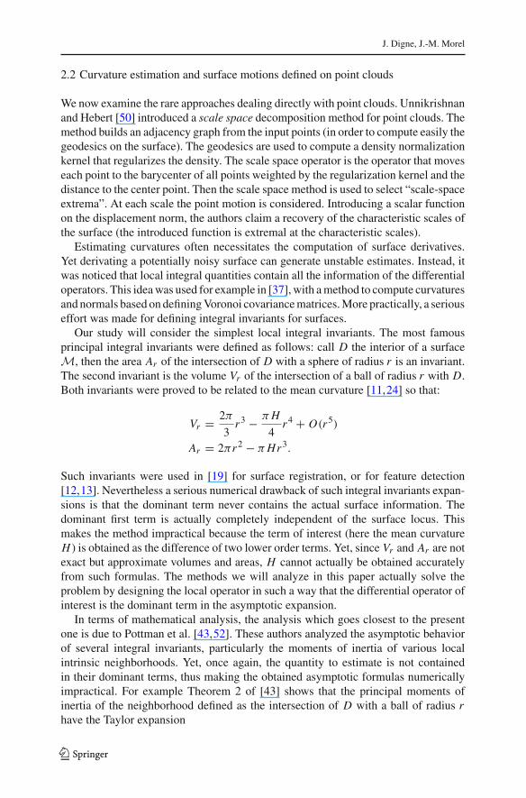
2.2 Curvature estimation and surface motions defined on point clouds

We now examine the rare approaches dealing directly with point clouds. Unnikrishnanand Hebert [50] introduced a scale space decomposition method for point clouds. Themethod builds an adjacency graph from the input points (in order to compute easily thegeodesics on the surface). The geodesics are used to compute a density normalizationkernel that regularizes the density. The scale space operator is the operator that moveseach point to the barycenter of all points weighted by the regularization kernel and thedistance to the center point. Then the scale space method is used to select “scale-spaceextrema”. At each scale the point motion is considered. Introducing a scalar functionon the displacement norm, the authors claim a recovery of the characteristic scales ofthe surface (the introduced function is extremal at the characteristic scales).

Estimating curvatures often necessitates the computation of surface derivatives.Yet derivating a potentially noisy surface can generate unstable estimates. Instead, itwas noticed that local integral quantities contain all the information of the differentialoperators. This idea was used for example in [37], with a method to compute curvaturesand normals based on defining Voronoi covariance matrices. More practically, a seriouseffort was made for defining integral invariants for surfaces.

Our study will consider the simplest local integral invariants. The most famousprincipal integral invariants were defined as follows: call D the interior of a surfaceM, then the area Ar of the intersection of D with a sphere of radius r is an invariant.The second invariant is the volume Vr of the intersection of a ball of radius r with D.Both invariants were proved to be related to the mean curvature [11,24] so that:

Vr = 2π

3r3 − π H

4r4 + O(r5)

Ar = 2πr2 − π Hr3.

Such invariants were used in [19] for surface registration, or for feature detection[12,13]. Nevertheless a serious numerical drawback of such integral invariants expan-sions is that the dominant term never contains the actual surface information. Thedominant first term is actually completely independent of the surface locus. Thismakes the method impractical because the term of interest (here the mean curvatureH ) is obtained as the difference of two lower order terms. Yet, since Vr and Ar are notexact but approximate volumes and areas, H cannot actually be obtained accuratelyfrom such formulas. The methods we will analyze in this paper actually solve theproblem by designing the local operator in such a way that the differential operator ofinterest is the dominant term in the asymptotic expansion.

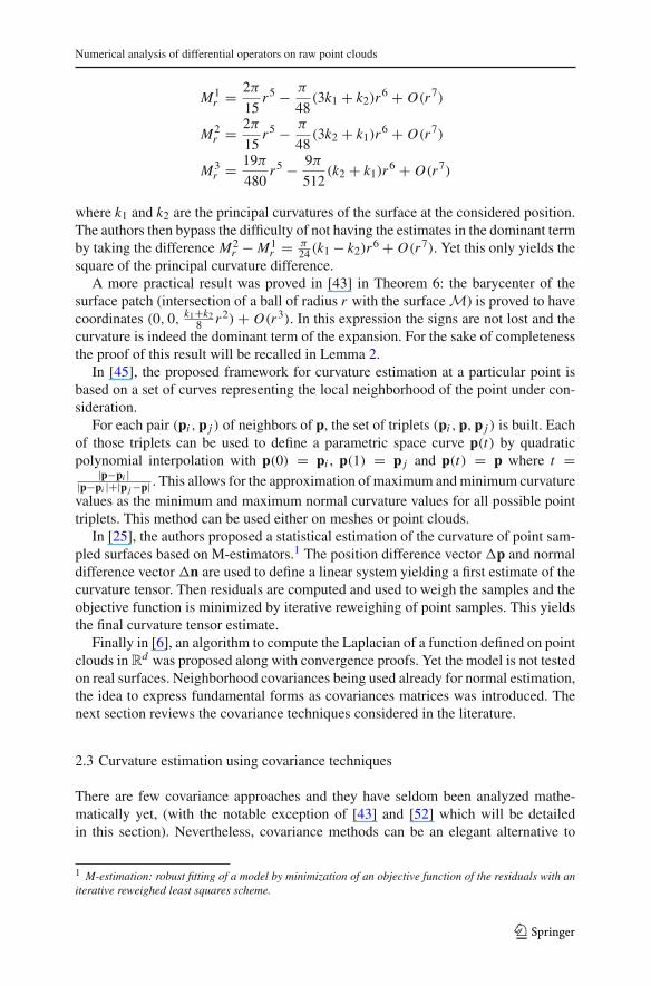
In terms of mathematical analysis, the analysis which goes closest to the presentone is due to Pottman et al. [43,52]. These authors analyzed the asymptotic behaviorof several integral invariants, particularly the moments of inertia of various localintrinsic neighborhoods. Yet, once again, the quantity to estimate is not containedin their dominant terms, thus making the obtained asymptotic formulas numericallyimpractical. For example Theorem 2 of [43] shows that the principal moments ofinertia of the neighborhood defined as the intersection of D with a ball of radius rhave the Taylor expansion

123

Numerical analysis of differential operators on raw point clouds

M1r = 2π

15r5 − π

48(3k1 + k2)r

6 + O(r7)

M2r = 2π

15r5 − π

48(3k2 + k1)r

6 + O(r7)

M3r = 19π

480r5 − 9π

512(k2 + k1)r

6 + O(r7)

where k1 and k2 are the principal curvatures of the surface at the considered position.The authors then bypass the difficulty of not having the estimates in the dominant termby taking the difference M2

r − M1r = π

24 (k1 − k2)r6 + O(r7). Yet this only yields thesquare of the principal curvature difference.

A more practical result was proved in [43] in Theorem 6: the barycenter of thesurface patch (intersection of a ball of radius r with the surface M) is proved to havecoordinates (0, 0, k1+k2

8 r2) + O(r3). In this expression the signs are not lost and thecurvature is indeed the dominant term of the expansion. For the sake of completenessthe proof of this result will be recalled in Lemma 2.

In [45], the proposed framework for curvature estimation at a particular point isbased on a set of curves representing the local neighborhood of the point under con-sideration.

For each pair (pi , p j ) of neighbors of p, the set of triplets (pi , p, p j ) is built. Eachof those triplets can be used to define a parametric space curve p(t) by quadraticpolynomial interpolation with p(0) = pi , p(1) = p j and p(t) = p where t =

|p−pi ||p−pi |+|p j −p| . This allows for the approximation of maximum and minimum curvaturevalues as the minimum and maximum normal curvature values for all possible pointtriplets. This method can be used either on meshes or point clouds.

In [25], the authors proposed a statistical estimation of the curvature of point sam-pled surfaces based on M-estimators.1 The position difference vector �p and normaldifference vector �n are used to define a linear system yielding a first estimate of thecurvature tensor. Then residuals are computed and used to weigh the samples and theobjective function is minimized by iterative reweighing of point samples. This yieldsthe final curvature tensor estimate.

Finally in [6], an algorithm to compute the Laplacian of a function defined on pointclouds in R

d was proposed along with convergence proofs. Yet the model is not testedon real surfaces. Neighborhood covariances being used already for normal estimation,the idea to express fundamental forms as covariances matrices was introduced. Thenext section reviews the covariance techniques considered in the literature.

2.3 Curvature estimation using covariance techniques

There are few covariance approaches and they have seldom been analyzed mathe-matically yet, (with the notable exception of [43] and [52] which will be detailedin this section). Nevertheless, covariance methods can be an elegant alternative to

1 M-estimation: robust fitting of a model by minimization of an objective function of the residuals with aniterative reweighed least squares scheme.

123

J. Digne, J.-M. Morel

surface regression. Three papers [7,33,40] use covariance matrices for the curvatureestimation.

The first one [7] considers the neighbors (pi ) of a point p. The second fundamentalform analog is then defined as the covariance matrix of the vectors ppi projected ontothe tangent plane of the surface at p. An analog of the Gauss map is also introduced:it is the covariance matrix of the neighbors unit normals projected onto the surfacetangent plane at point p. The eigenvectors are said to give the principal directions. Infact these two covariance matrices are inspired from [33]. Indeed, [33] first proposedto compute the covariance matrix of the normals at the neighbors of p, and to extractthe principal eigenvalues which correspond to the principal curvatures of the surfaceat p. The last covariance method, introduced in [40] is not claimed to be explicitlylinked to surface curvatures or fundamental forms, yet it is used to account for thesurface geometric variations. Consider the covariance matrix of vectors opi where o isthe barycenter of the neighborhood of p. The surface variation is defined as the ratioof the least eigenvector over the sum of all eigenvectors of this covariance matrix.This quantity has the nice property that it is bounded between 0 (flat case) and 1/3(isotropic case). All of these methods will be detailed and analyzed in Sect. 4.

2.4 Moving least squares surfaces

Moving least square (MLS) surfaces were introduced in [30] as follows. Given a dataset of points {pi }i (possibly acquired by a 3D scanning device) and belonging to asmooth surface M, the goal is to replace the points p defining M by a reduced setR = {ri } defining a so called MLS M′ surface which approximates M. The surfaceM is assumed to be a C∞ 2-manifold. The authors fix a bounding error ε such thatd(M,M′) < ε, where d is the Hausdorff distance.

The projection of a point on the MLS surface is defined as follows: given a point p,find a local reference domain (plane) for p. The local regression plane H is obtained byminimizing a local weighted sum of square distances of the points pi to the plane. Theweights attached to pi are defined as functions of the distance of pi to the projectionof p on plane H , rather than their distance to p.

Assume Q is the projection of p onto H , then H is found by locally minimizingwith respect to n and D the quadratic cost

N∑

i=1

(〈n, pi 〉 − D)2θ(‖pi − Q‖)

where θ is a smooth, monotone decreasing positive function. We can set Q = p + tnfor some t ∈ R, which leads to the minimization of

N∑

i=1

(〈n, pi − p − tn〉)2θ(‖pi − p − tn‖).

The local reference domain is then given by an orthonormal coordinate system onH with origin Q. The reference domain for p is used to compute a local bivariate

123

Numerical analysis of differential operators on raw point clouds

polynomial approximation to the surface in a neighborhood of p. Let Qi be theprojection of pi onto H , and fi = 〈n, pi − Qi 〉. In this local coordinate system,let (xi , yi ) be the coordinates of Qi on H . The coefficients of the polynomial arecomputed by minimizing the least square error

∑Ni=1(g(xi , yi ) − fi )

2θ(‖pi − Q‖).The projection of p onto M is defined by the polynomial value at the origin, i.e.Q + g(0, 0)n = p + (t + g(0, 0))n. Thus, given a point p and its neighborhood, itsprojection onto the MLS surface can be computed. The approximation power of MLSsurfaces was evaluated in [31] and the first applications were introduced in [2,5,32].

MLS surfaces are not only theoretically powerful; they also provide fine implemen-tations for rendering, up-sampling or down-sampling point sets [3,40]. Finer variantsof MLS were subsequently proposed for a better preservation of sharp edges in surfacesdefined by point clouds [1,18,21,34,39].

The same framework was used to build a scale space for point clouds in [41]. Thesurface is evolved through a diffusion process ∂p

∂t − λ · �p = 0, where p is a point ofthe surface, λ a diffusion parameter and �p = Hn is the Laplace Beltrami Operator(H is the curvature and n the normal at point p, this is the decomposition process). Byremembering the set of displacements Di (p) of each point p we have a reconstructionoperator. The choice of the Laplacian discretization is very important: a first possibilityis to use the standard mesh Laplacian techniques [47] adapted for point clouds usingthe k-nearest neighbors instead of the one ring neighborhood. Another possibility is touse the weighted least squares projection [23,26] : the surface is iteratively projectedonto the plane defined by the weighted barycenter o and the normal estimated usingthe weighted neighborhood covariance matrix. The weights are a Gaussian functionof the distance to p, and the size of the Gaussian kernel is a parameter that controls theamount of smoothing. This projection process is in fact an order 1 projection motion(MLS1) that will be analyzed in the following sections.

To make the projection more efficient, Pauly et al. [41] proposed to sub-samplethe point cloud. This yields a scale space decomposition where at each level thesurface is smoothed and sub-sampled. The scale space decomposition is then appliedto the multi-scale freeform deformation and to the morphing problem, with satisfactoryresults.

The MLS were used to estimate curvatures. For example, in [51], the authors usethe MLS framework to build a closed form solution for curvature estimation. Indeed,surfaces implied by point clouds can be seen as the zero level set of an implicit functionf whose gradient and Hessian Matrix are built. Finally, using formulas for the Gaussianand the mean curvature depending on the Hessian and gradient of f , those curvaturescan be computed.

In [10], the problem of estimating differential quantities on point clouds is recast tothat of fitting the local representation of the manifold by a jet. A jet is simply a truncatedTaylor expansion. A n jet is a Taylor expansion truncated at order n. A jet of order ncontains differential information up to the n-th order. In particular it is stated that apolynomial fitting of degree n estimates any kth order differential quantity to accuracyO(hn−k+1). This implies that the coefficient of the first fundamental form and unitvector normal are estimated with O(hn) precision and the coefficients of the secondfundamental form and shape operator are approximated with accuracy O(hn−1), and

123

J. Digne, J.-M. Morel

so are the principal directions. In order to characterize curvature properties, the methodresorts to the Weingarten map A of the surface, also called the shape operator, that isthe tangent map of the Gauss map. Recall that the first and second fundamental formsI , I I and A satisfy I I (t, t) = I (A(t), t) for any vector t of the tangent space. Secondorder derivatives are computed by building the Weingarten map of the osculating jetwhose eigenvalues are the principal curvatures. Note that the described methods canbe used either with a mesh or with a point cloud. Jets are in fact very related to MLSsurfaces. Indeed, to estimate differential quantities a polynomial fitting of degree n isdone, which is exactly what MLS does. Therefore the analysis in Sect. 5 giving theequation governing MLS1 and MLS2 motions are valid for the jets too.

Nevertheless, we shall prove that none of the above mentioned moment based meth-ods for computing the curvatures without a surface regression gives back the signedcurvatures. We shall also prove experimentally that in order to be stable, those integralestimates as well as the surface regression estimates require a large neighborhood,which leads to larger computation time. In terms of signal-to-noise ratio, it will turnout to be better to consider a scale-space approach: applying the scale space iterationswith a small neighborhood and then extracting the differential operator analogue.

This section has reviewed the main methods aiming at estimating locally the sur-face shape, thus implicitly computing local equivalents of the infinitesimal curvaturetensor. We have seen that two sorts of methods, logically, dominate: the polynomialregressions on one side, and the local moments on the other. (It is actually difficult toimagine other kinds of local methods on a raw point set). These kinds have very dif-ferent techniques, but we shall be able to compare them in two unifying frameworks.We shall first give their asymptotic equivalents, which are functions of the surfaceprincipal curvatures. Then we shall compare their reliability by a numerical set up inthe experimental section.

In particular Sect. 4 finds the form of the differential operators underlying the fourmentioned discrete schemes based on local cloud point statistics, and proposing dis-crete analogues of the “second fundamental forms” or of the “principal curvatures”.These discrete schemes have very simple and robust form, being based on the compu-tation of local moments and eigenvalues of the point cloud. The next Sect. 3 providesthe tools to analyze numerically point cloud motions. The analysis is in spirit close tothe image filter analysis performed in [8].

3 Tools for numerical analysis of point cloud surface motions

We always assume the existence of a smooth surface M supporting the point set. Thesesurfaces are the boundaries of solid objects and can therefore be assumed to be locallyLipschitz graphs. However, for a mathematical analysis of smoothing algorithms andcurvature estimations on the surface, we shall always assume that the surface is a C∞embedded manifold, known from its samples denoted by MS . This is not a limitation,in the sense that any finite sample set can be anyway interpolated by an arbitrarilysmooth surface. Let p = p(xp, yp, zp) be a point of the surface M. At each nonumbilical point p, consider the principal curvatures k1 and k2 linked to the principaldirections t1 and t2, with k1 > k2 where t1 and t2 are orthogonal vectors. At umbilical

123

Numerical analysis of differential operators on raw point clouds

Spherical Neighborhood

Regression Plane

Cylindrical Neighborhood

Fig. 1 Comparison between cylindrical and spherical neighborhoods

points, any orthogonal pair (t1, t2) can be taken. Set n = t1 × t2 so that (t1, t2, n) is anorthonormal basis. The quadruplet (p, t1, t2, n) is called the local intrinsic coordinatesystem. In this system we can express locally the surface as a C2 graph z = f (x, y)

(Fig. 1). By Taylor expansion,2

z = f (x, y) = 1

2

(k1x2 + k2 y2

)+ o

(x2 + y2

). (1)

Notice that the sign of the pair (k1, k2) depends on the arbitrary surface orientation.Points where k1 and k2 have the same sign are called parabolic, and points where theyhave opposite signs are hyperbolic.

Consider two kinds of neighborhoods in M for p defined in the local intrinsiccoordinate system (p, t1, t2, n) (see Fig. 1):

– the spherical neighborhood Br = Br (p) ∩ M is the set of all points m of M withcoordinates (x, y, z) satisfying (x − xp)2 + (y − yp)2 + (z − zp)2 < r2

– the cylindrical neighborhood Cr = Cr (p) ∩ M is the set of all points m(x, y, z)on M such that (x − xp)2 + (y − yp)2 < r2.

The spherical neighborhood in the sampled surface MS is the only neighborhood towhich there is a direct numerical access. It serves for defining all numerical schemesconsidered here. Nevertheless, for the forthcoming asymptotic numerical analysis, thecylindrical neighborhood will prove much handier than the spherical one. The nexttechnical lemma justifies its use in theoretical calculations.

2 We could use z = f (x, y) = − 12 (k1x2 + k2 y2)+ o(x2 + y2) at the cost of changing the orientation and

sign of k1, k2.

123

J. Digne, J.-M. Morel

Lemma 1 Integrating on M any function f (x, y) such that f (x, y) = O(rn) on acylindrical neighborhood Cr instead of a spherical neighborhood Br introduces ano(rn+4) error. More precisely:

∫

Br

f (x, y)dm =∫

x2+y2<r2

f (x, y)dxdy + O(r4+n). (2)

Proof The surface area element of a point m(x, y, z(x, y)) on the surface M,

expressed as a function of x , y, dx and dy is dm(x, y) =√

1 + z2x + z2

ydxdy. One

has zx = k1x + O(r2) and zy = k2 y + O(r2). Thus

dm(x, y) =√(

1 + k21 x2 + k2

2 y2 + O(r3))dxdy

which yields

dm(x, y) =(

1 + O(r2))

dxdy. (3)

Using (3), the integrals we are interested in become

∫

Br

f (x, y)dm = (1 + O(r2))

∫

x2+y2+z2<r2,(x,y,z)∈Mf (x, y)dxdy; (4)

∫

Cr

f (x, y)dm = (1 + O(r2))

∫

x2+y2<r2, (x,y,z)∈Mf (x, y)dxdy. (5)

The right hand forms are amenable to analytic computations. Consider polar coor-dinates (ρ, θ) such that x = ρ cos θ and y = ρ sin θ with −r ≤ ρ ≤ rand 0 ≤ θ ≤ π . Then for m(x, y, z) belonging to the surface M, we havez = 1

2ρ2(k1 cos2 θ + k2 sin2 θ) + O(r3). Thus z = 12ρ2k(θ) + O(r3), where

k(θ) = k1 cos2 θ + k2 sin2 θ . The condition that (x, y, z) belongs to the neighbor-hood Br can therefore be rewritten as ρ2 + z2 < r2, that is

ρ2 + 1

4k(θ)2ρ4 < r2 + O(r5).

Computing the boundaries ±ρ(θ) of this neighborhood yields ρ(θ)2 + 14 k(θ)2ρ(θ)4 −

r2 + O(r5) = 0. Thus

ρ(θ)2 =−1 +

√1 + k(θ)2

(r2 + O(r5)

)

12 k(θ)2

.

123

Numerical analysis of differential operators on raw point clouds

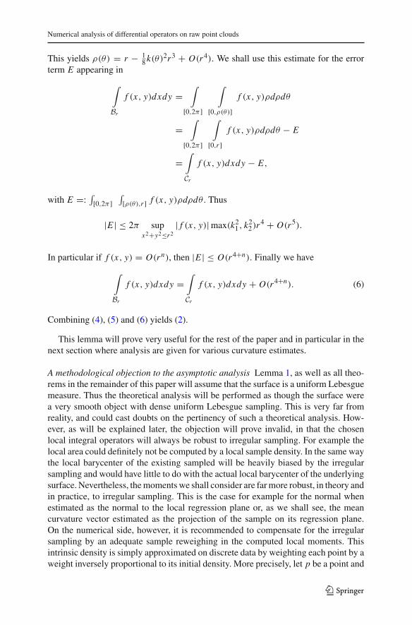
This yields ρ(θ) = r − 18 k(θ)2r3 + O(r4). We shall use this estimate for the error

term E appearing in

∫

Br

f (x, y)dxdy =∫

[0,2π ]

∫

[0,ρ(θ)]f (x, y)ρdρdθ

=∫

[0,2π ]

∫

[0,r ]f (x, y)ρdρdθ − E

=∫

Cr

f (x, y)dxdy − E,

with E =: ∫[0,2π ]

∫[ρ(θ),r ] f (x, y)ρdρdθ . Thus

|E | ≤ 2π supx2+y2≤r2

| f (x, y)| max(k21, k2

2)r4 + O(r5).

In particular if f (x, y) = O(rn), then |E | ≤ O(r4+n). Finally we have

∫

Br

f (x, y)dxdy =∫

Cr

f (x, y)dxdy + O(r4+n). (6)

Combining (4), (5) and (6) yields (2).

This lemma will prove very useful for the rest of the paper and in particular in thenext section where analysis are given for various curvature estimates.

A methodological objection to the asymptotic analysis Lemma 1, as well as all theo-rems in the remainder of this paper will assume that the surface is a uniform Lebesguemeasure. Thus the theoretical analysis will be performed as though the surface werea very smooth object with dense uniform Lebesgue sampling. This is very far fromreality, and could cast doubts on the pertinency of such a theoretical analysis. How-ever, as will be explained later, the objection will prove invalid, in that the chosenlocal integral operators will always be robust to irregular sampling. For example thelocal area could definitely not be computed by a local sample density. In the same waythe local barycenter of the existing sampled will be heavily biased by the irregularsampling and would have little to do with the actual local barycenter of the underlyingsurface. Nevertheless, the moments we shall consider are far more robust, in theory andin practice, to irregular sampling. This is the case for example for the normal whenestimated as the normal to the local regression plane or, as we shall see, the meancurvature vector estimated as the projection of the sample on its regression plane.On the numerical side, however, it is recommended to compensate for the irregularsampling by an adequate sample reweighing in the computed local moments. Thisintrinsic density is simply approximated on discrete data by weighting each point by aweight inversely proportional to its initial density. More precisely, let p be a point and

123

J. Digne, J.-M. Morel

Nr (p) = Ms ∩ Br (p). Each point q should ideally have a weight 0 ≤ w(q) ≤ 1 suchthat

∑q∈Nr (p) w(q) = 1. This amounts to solve a huge linear system. For this reason,

we shall be contented in the experimental section with ensuring∑

q∈Nr (p) w(q) 1

by taking w(p) = 1�(Bp(r))

, as proposed in [50].

4 Curvature estimates by covariance matrix methods

This section contains some of the main contributions of the present paper. It finds theform of the differential operators underlying four different discrete schemes based onlocal cloud point statistics, and proposing discrete analogues of the “second funda-mental form matrix” or of the “principal curvatures”. These discrete schemes have avery simple and robust form, being based on the computation of local moments andeigenvalues of the point cloud or of its normals. We shall see that all of the meth-ods asymptotically compute nonlinear differential operators linked to the principalcurvatures. Their principle is to replace the matrix of the second fundamental formby some symmetric matrix that can be deduced from the local statistics of the pointcloud. We shall consider four matrices (2 or 3-dimensional) that are the simplest ofsuch covariance matrices:

– 2D covariance matrix of the projections of −→pi p on the tangent plane where pi arethe points of the neighborhood (Sect. 4.1);

– 2D covariance matrix of the projections of the unit normals n(pi ) on the tangentplane (Sect. 4.2);

– 3D covariance matrix of the unit normals n(pi ) (Sect. 4.3);– 3D centered covariance matrix of the −→pi o where o is the barycenter of the neigh-

borhood (Sect. 4.4).

4.1 A discrete “second fundamental form” [7]

Let (pi )i∈1...N be the set of neighbors of a point p with normal n. This paper proposesto build the “second fundamental form matrix” as follows. Although this covariancematrix is not, as we shall see, consistent with the second fundamental form, it is thuscalled in this paper, and actually has asymptotically, as we shall see, the principaldirections as eigenvectors. Let si = (pi −p)T ·n, let t1, t2 be two orthonormal vectorsin the tangent plane of p, and

αi = si ·(

(pi − p) · t1(pi − p) · t2

)

= ((pi − p)T · n) ·(

(pi − p) · t1(pi − p) · t2

)

.

The αi are the projections of the vectors (pi −p) onto the tangent plane to p, weightedby their distance to this plane. The “second fundamental form matrix” is the covarianceof these vectors, namely

123

Numerical analysis of differential operators on raw point clouds

Σd =N∑

i=1

(αi − αm) · (αi − αm)T (7)

where αm = 1N

∑Ni=1 αi and in Σd the d stands for “discrete”. To compute the

underlying differential operators, two assumptions will be made throughout this paper.The first one is that the surface sampling is uniform with respect to the area measure onthe surface. The second one is that this sampling is dense enough, so that the averagestaken on neighborhoods can be interpreted as integrals. Under this interpretation,we can reinterpret the sum in (7) as an integral on a cylindrical neighborhood of p,assuming the data point set to be a locally smooth manifold. In the local intrinsicsurface coordinate system at point p, (p, t1, t2, n), the surface can be written as agraph z = 1

2 (k1x2 + k2 y2) + o(r2). Thus the vectors αi are replaced by a continuousvector α(x, y) defined by

α(x, y) = 1

2(k1x2 + k2 y2) ·

(xy

)

= 1

2·(

k1x3 + k2 y2xk1x2 y + k2 y3

)

+ o(r3). (8)

Under the interpretation taken above the “second fundamental matrix” rewrites

Σ =∫

Br

(α(x, y) − αm) · (α(x, y) − αm)T dm(x, y) (9)

where

αm = 1

meas(Br )

∫

Br

α(x, y)dm(x, y). (10)

The proposition made in [7] is to extract the surface principal curvatures and theircorresponding directions at p from this covariance matrix, as its eigenvalues andeigenvectors. The next theorem checks if this works asymptotically in the continuousmodel.

Theorem 1 The eigenvectors of the “second fundamental form matrix” Σ give theprincipal directions with error o(r8). But the eigenvalues of Σ are not the principalcurvatures as they satisfy

λ1 = πr8

256

(5k2

1 +2k1k2+k22)+o(r8

)and λ2 = πr8

256

(k2

1 + 2k1k2 + 5k22

)+ o(r8)

where k1 and k2 are the principal curvatures at p

Proof In the continuous model αm therefore is close to zero because the integratedfunction is odd on a symmetric domain. More precisely, using Lemma 1 in (10) andwriting αm = (αmx , αmy),

123

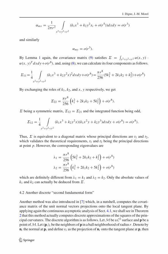
J. Digne, J.-M. Morel

αmx = 1

2πr2

∫

x2+y2<r2

(k1x3 + k2 y2xi + o(r5))dxdy = o(r3)

and similarly

αmy = o(r3).

By Lemma 1 again, the covariance matrix (9) satisfies Σ = ∫x2+y2<r2 α(x, y) ·

α(x, y)T dxdy+o(r8), and, using (8), we can calculate its four components as follows.

Σ11 = 1

4

∫

x2+y2<r2

(k1x3 + k2 y2x)2dxdy+o(r8)= πr8

256(5k2

1 + 2k1k2 + k22)+o(r8)

By exchanging the roles of k1, k2, and x , y respectively, we get

Σ22 = πr8

256

(k2

1 + 2k1k2 + 5k22

)+ o(r8).

Σ being a symmetric matrix, Σ12 = Σ21 and the integrated function being odd,

Σ12 = 1

4

∫

x2+y2<r2

(k1x3 + k2 y2x)(k1x2 y + k2 y3)dxdy + o(r8) = o(r8).

Thus, Σ is equivalent to a diagonal matrix whose principal directions are t1 and t2,which validates the theoretical requirements, t1 and t2 being the principal directionsat point p. However, the corresponding eigenvalues are

λ1 = πr8

256

(5k2

1 + 2k1k2 + k22

)+ o(r8)

λ2 = πr8

256

(k2

1 + 2k1k2 + 5k22

)+ o(r8)

which are definitely different from λ1 = k1 and λ2 = k2. Only the absolute values ofk1 and k2 can actually be deduced from Σ .

4.2 Another discrete “second fundamental form”

Another method was also introduced in [7] which, in a nutshell, computes the covari-ance matrix of the unit normal vectors projections onto the local tangent plane. Byapplying again the continuous asymptotic analysis of Sect. 4.1, we shall see in Theorem2 that this method actually computes discrete approximations of the squares of the prin-cipal curvatures. The discrete algorithm is as follows. Let M be a C2 surface and p be apoint ofM. Let (pi )i be the neighbors of p in a ball neighborhood of radius r . Denote byni the normal at pi and define vi as the projection of ni onto the tangent plane at p, then

123

Numerical analysis of differential operators on raw point clouds

the computed “curvatures” are defined as the eigenvalues of the covariance matrix ofthe vectors vi . The vector vi being the projection of ni onto the tangent plane, we have

vi =(

ni · t1ni · t2

)

.

Set vm = 1N

∑Ni=1 vi . Then this new discrete covariance matrix writes Σd =∑N

i=1(vi−vm) · (vi −vm)T . In the continuous framework, the local points on the surface havecoordinates m(x, y) = (x, y, 1

2 (k1x2 +k2 y2)+o(r2)) and the normal vector to thissurface is ∂m

∂x (x, y) ∧ ∂m∂y (x, y)=(−k1x,−k2 y, 1) + o(r). It follows that

v(x, y) = 1√

1 + k21 x2 + k2

2 y2

(−k1x−k2 y

)

+ o(r),

vm = 1

meas(Br )

∫

v(x, y)dm(x, y),

and the continuous covariance matrix is

Σ :=∫

Br

(v(x, y) − vm) · (v(x, y) − vm)T .

Theorem 2 The eigenvalues of the covariance matrix Σ of the vectors v(x, y) in thespherical neighorhood Br are

k21r4π

4+ o(r4) and

k22r4π

4+ o(r4).

Proof Let us compute the mean vm of v(x, y) on the spherical neighborhood. ByLemma 1 the integral on a spherical neighborhood is asymptotically equivalent to theintegral on a cylindrical neighborhood and more precisely, (πr2)vm · t1 = o(r3) andsimilarly

(πr2)vm · t2 =∫

x2+y2<r2

−k2 y√

1 + k21 x2 + k2

2 y2dxdy + o(r4) = o(r3).

Thus the coefficients of Σ satisfy, again by Lemma 1,

Σ11 =∫

x2+y2<r2

k21 x2

1 + k21 x2 + k2

2 y2dxdy + o(r4) =

∫

x2+y2<r2

k21 x2 + o(r4)

= k21r4π

4+ o(r4)

Similarly, Σ22 = k22r4π

4 + o(r4) and Σ12 = Σ21 = o(r4).

123

J. Digne, J.-M. Morel

Thus Σ is asymptotically diagonal and its eigenvalues Σ11 and Σ22 are asymptot-ically obtained for the principal directions t1 and t2. Yet, these eigenvalues asymptot-ically give an approximation of each one of the squared principal curvatures, but notof their sign.

4.3 A third discrete “fundamental form”

The methods analyzed in Sects. 4.1 and 4.2 are akin to the original method introducedin [33]. Indeed, in [33] it was proposed to compute the covariance matrix of the normalvectors of the neighborhood (without projecting them in the local regression plane)and therefore get a 3 × 3 matrix instead of a 2 × 2 matrix. This is actually the simplestimaginable method and we shall see that it gives a result similar to Sect. 4.2.

Theorem 3 Let M be a C2 surface, let p be a point of M. Then the three eigenvaluesof the covariance matrix C of the unit normals in a neighborhood of radius r around pare asymptotically respectively equal to 1 and to the squares of the principal curvaturesat p.

Proof A normal vector writes

N = 1√

1 + k21 x2 + k2

2 y2

⎛

⎝−k1x−k2 y

1

⎞

⎠ + o(r).

As in the previous sections, we easily obtain by Lemma 1, Nmx = o(r), Nmy =o(r), Nmz = 1 + o(r). Thus again by Lemma 1,

C =∫

x2+y2≤r2

1

1+k21 x2+k2

2 y2

⎛

⎝k2

1 x2 k1k2xy k1x(1−Nmz)

k1k2xy k22 y2 k2 y(1−Nmz)

k1x(1−Nmz) k2 y(1−Nmz) (1−Nmz)2

⎞

⎠dxdy+o(r4)

and, by calculations exactly analogous to Sect. 4.2, C11 = k21r4π

4 + o(r4), C22 =k2

2r4π

4 + o(r4), C12 = C21 = k1k2∫

x,y xydxdy = o(r4), C13 = C31 = C23 = C32 =C33 = o(r4).

Thus the eigenvalues are asymptotically equal tok2

1r4π

4 andk2

2r4π

4 , which alsogives back the squares of the principal curvatures of the surface, but again not theirsign.

4.4 A fourth discrete fundamental form: the surface variation

We shall now analyze a last variant introduced in [40], the so called surface variation.It is again based on a local covariance analysis. Unlike the previous methods, thesurface variation was not claimed to be a curvature estimate, but to be a measure of

123

Numerical analysis of differential operators on raw point clouds

the neighborhood shape. This subsection establishes again a link between this discretequantity and the principal curvatures of the surface.

Let p be a point with given neighborhood Br . Let o be the barycenter of the neigh-borhood. In R

3, the coordinates are written with superscripts e.g. the coordinates of apoint u are (u1, u2, u3). Thus, for i = 1, 2, 3, oi = 1

card Br

∑pk∈Br

pik . The centered

covariance matrix Σ = (mi j )i, j=1,...,3 is defined as mi j = ∑pk∈Br

(pik −oi )·(p j

k −o j )

for i, j = 1, 2, 3. Let λ0 ≤ λ1 ≤ λ2 be the eigenvalues of Σ with corresponding eigen-vectors v0, v1, v2. For k = 0, . . . , 2,

λk =∑

pi ∈Br

〈(pi − o), vk〉2. (11)

Each eigenvalue gives the variance of the point set in the direction of the correspondingeigenvector. Since v1 and v2 are the vectors that capture most variations, they definethe PCA regression plane. The normal v0 to this plane is the direction v minimizing∑

pi ∈Br〈(pi − o), v〉2. Pauly et al. [40] defines the surface variation by

σ = λ0

λ0 + λ1 + λ2. (12)

This quantity measures the ratio of variance along the normal to the total variance.If the neighborhood is highly curved, its surface variation will be high and if theneighborhood is flat the surface variation will be small. This quantity has the propertyto be bounded between 0 (flat case) and 1/3 (isotropic distribution case).

Lemma 2 (Pottmann et al. [43]) In the local intrinsic coordinate system, the barycen-ter of a neighborhood Br of point p has coordinates xo = o(r2), yo = o(r2) and

zo = Hr2

4 + o(r2), where H = k1+k22 is the mean curvature at p.

Proof We give the proof for the sake of completeness. By Lemma 1 applied to thenumerator and denominator of the following fraction, we have

zo =∫Br

zdm∫Br

dm=

∫x2+y2<r2 z(x, y)dxdy + O(r5)

∫x2+y2<r2 dxdy + O(r3)

=∫

x2+y2<r2

[ 12 (k1x2 + k2 y2) + o(x2 + y2)

]dxdy

∫x2+y2<r2 dxdy

+ O(r3)

= 1

2πr2

r∫

ρ=0

2π∫

θ=0

ρ2(k1 cos2 θ + k2 sin2 θ)ρdρdθ + o(r2)

= r2

8π(k1π + k2π) + o(r2) = Hr2

4+ o(r2).

A similar but simpler computation yields the estimates of xo and yo.

123

J. Digne, J.-M. Morel

Theorem 4 In the local coordinate system the surface variation σ satisfies

σ = r2

16

(k2

1 + k22

2− 1

3k1k2

)

+ o(r2) (13)

Proof We need to explain what the covariance eigenvalues stand for. Each eigenvectorvi and associated eigenvalue λi represent a principal direction and the variation alongthis principal direction,

λi =∫

m∈Br

〈om, vi 〉2dm.

Since we have λ0 ≤ λ1 ≤ λ2, we can see that λ0 is associated to the direction with theleast variation namely the normal direction to the surface oz. Since the eigenvectorsform an orthonormal basis, we have

λ0 + λ1 + λ2 =∫

m∈Cr

〈om, v0〉2 + 〈om, v1〉2 + 〈om, v2〉2dm =∫

m∈Cr

‖om‖2dm

This yields λ0 + λ1 + λ2 =∫

x2+y2<r2x2 + y2 + (z − zo)

2dxdy and

λ0 + λ1 + λ2 = πr4

2+ λ0 + o(r6) (14)

We first compute λ0, applying again Lemma 1 to get back to the easy cylindricalneighborhood.

λ0 =∫

x2+y2≤r2

(z − zo)2dxdy

=∫

x2+y2≤r2

z2dxdy + z2o

∫

x2+y2≤r2

dxdy − 2zo

∫

x2+y2≤r2

zdxdy

=∫

x2+y2≤r2

z2dxdy + H2r4

16× πr2 − 2

Hr2

4

r4

4π H + o(r6)

= 1

4(k2

1

∫

x2+y2≤r2

x4dxdy + k22

∫

x2+y2≤r2

y4dxdy + 2k1k2

∫

x2+y2≤r2

x2 y2dxdy

− H2r6

16π + o(r6)

= 1

4

r6

6

(3π

4(k2

1 + k22) + k1k2

π

2

)

− H2r6

16π + o(r6)

123

Numerical analysis of differential operators on raw point clouds

where H = k1+k22 is the mean curvature. Thus

λ0 = πr6

32

(k2

1 + k22

2− 1

3k1k2

)

+ o(r6) (15)

Using (14) and (15) we get

σ =r2

16

(k2

1+k22

2 − 13 k1k2

)

+ o(r2)

1 + r2

16

(k2

1+k22

2 − 13 k1k2

)

+ o(r2)

which finally yields:

σ = r2

16

(k2

1 + k22

2− 1

3k1k2

)

+ o(r2)

The formula of the surface variation given by Theorem 4 indeed measures a sort ofcurvature. To interpret it we can notice that

– the surface variation is symmetric in k1, k2;– in the case of a point lying on a sphere, k1 = k2 = k so σsphere = r6

24 k2;

– in the case of a saddle point k1 = k = −k2, σsaddle = r6

12 k2 so σsphere < σsaddle;

– in the case of a cylinder k1 = k, k2 = 0, σcylinder = r6

32 k2.

It follows from that the surface variation is not a discriminating enough informationabout the surface curvature. It is unable to discriminate very different local shapes.

5 Asymptotic behavior of MLS1 and MLS2

The simplest statistics that can be computed in a spherical neighborhood are thebarycenter and the regression plane. Lemma 2 stated that sending each point onto thebarycenter of its neighborhood approximates the mean curvature motion. The nextsimplest statistic is the regression plane, and the second next is the local degree 2regression surface. The main tool of the scale space proposed in [17] is the projectionof each surface point p on the local regression plane. This PCA regression plane isdefined as the plane orthogonal to the least eigenvector of the centered local covariancematrix, and passing through the centroid of the neighborhood. The projection of p onthis plane will be called p′ = M L S1(p) where MLSn stands for moving least squareof degree n. Indeed, this projection method is the simplest instance of the movingleast square method by which each point of a surface is projected to a local degree npolynomial regression. The local barycenter can actually be considered as an MLS oforder 0, MLS0. There is some particular interest in MLS1, because a recent meshingmethod uses it as the simplest reversible smoothing tool for point clouds [17]. On theother hand many cloud point processing methods involve some variant of the MLS2method to smooth, interpolate, or sub-sample a point cloud. MLS1 and MLS2 are

123

J. Digne, J.-M. Morel

smoothing operators and therefore could be used as scale spaces, that is, as iterativesmoothing operators. But, following [17] MLS1 indeed is a scale space. MLS2 is not,as illustrated in the experiments of Sect. 6. The theorems of this section clarify whathappens with these local polynomial regressions by first recalling briefly why MLS1implements a mean curvature motion, and second by showing that MLS2 is insensitiveto first, second, and third order intrinsic derivatives, and has an order 4 difference tothe original surface. The study reveals the fourth order intrinsic differential operatorassociated with MLS2.

5.1 The asymptotic behavior of MLS1

The next lemma compares the normal to the PCA regression plane with the normal tothe surface, n at p.

Lemma 3 The normal v to the PCA regression plane in a spherical neighborhoodBr at p ∈ M is equal to the surface normal at point p, up to a negligible factor:v = n + O(r).

Proof The local PCA regression plane of point p is characterized as the plane passingthrough the barycenter of the neighborhood Br and with normal v minimizing:

I (v) =∫

Br

|〈v, pp′〉|2dp′ s.t. ‖v‖ = 1

Denoting by (vx , vy, vz) the coordinates of v,

I (v) =∫

Br

(

vx x + vy y + vz1

2(k1x2 + k2 y2) + o(r2)

)2

dxdy.

Considering the particular value v = (0, 0, 1) shows that the minimal value Imin

of I (v) satisfies Imin ≤ O(r6). In consequence the minimum (vx , vy, vz) satisfiesvx ≤ O(r) and vy ≤ O(r). Thus, since ||v|| = 1, vz ≥ 1 − O(r) and thereforev = n + O(r).

Theorem 5 Let Tr be the operator defined on the surface M transforming each pointp into its projection p′ = Tr (p) on the local regression plane. Then

Tr (p) − p = Hr2

4n + o(r2). (16)

Proof By Lemma 2 the barycenter o of Br has local coordinates −→po = (o(r2), o(r2),Hr2

4 + o(r2)). On the other hand−→pp′ is proportional to the normal to the regression

plane, v. Thus by Lemma 3,−→pp′ = λ(O(r), O(r), 1 − O(r)). To compute λ, we use

the fact that p′ is the projection on the regression plane of p, and that o belongs to this

plane by definition. This implies that−→pp′ ⊥ −→

op′ and therefore

123

Numerical analysis of differential operators on raw point clouds

λ2 O(r2) + λ(1 − O(r))

(

Hr2

4+ o(r2) + λ(1 − O(r))

)

= 0,

which yields λ = Hr2

4 + o(r2) and therefore

−→pp′ =

(

O(r3), O(r3),Hr2

4+ o(r2)

)

= Hr2

4n + o(r2).

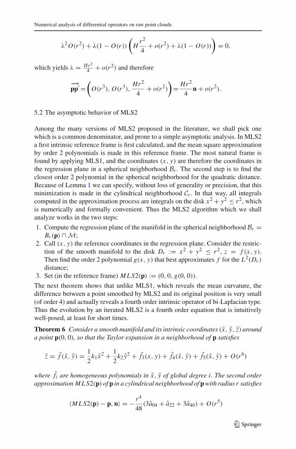
5.2 The asymptotic behavior of MLS2

Among the many versions of MLS2 proposed in the literature, we shall pick onewhich is a common denominator, and prone to a simple asymptotic analysis. In MLS2a first intrinsic reference frame is first calculated, and the mean square approximationby order 2 polynomials is made in this reference frame. The most natural frame isfound by applying MLS1, and the coordinates (x, y) are therefore the coordinates inthe regression plane in a spherical neighborhood Br . The second step is to find theclosest order 2 polynomial in the spherical neighborhood for the quadratic distance.Because of Lemma 1 we can specify, without loss of generality or precision, that thisminimization is made in the cylindrical neighborhood Cr . In that way, all integralscomputed in the approximation process are integrals on the disk x2 + y2 ≤ r2, whichis numerically and formally convenient. Thus the MLS2 algorithm which we shallanalyze works in the two steps:

1. Compute the regression plane of the manifold in the spherical neighborhood Br =Br (p) ∩ M;

2. Call (x, y) the reference coordinates in the regression plane. Consider the restric-tion of the smooth manifold to the disk Dr := x2 + y2 ≤ r2, z = f (x, y).Then find the order 2 polynomial g(x, y) that best approximates f for the L2(Dr )

distance;3. Set (in the reference frame) M L S2(p) := (0, 0, g(0, 0)).

The next theorem shows that unlike MLS1, which reveals the mean curvature, thedifference between a point smoothed by MLS2 and its original position is very small(of order 4) and actually reveals a fourth order intrinsic operator of bi-Laplacian type.Thus the evolution by an iterated MLS2 is a fourth order equation that is intuitivelywell-posed, at least for short times.

Theorem 6 Consider a smooth manifold and its intrinsic coordinates (x, y, z) arounda point p(0, 0), so that the Taylor expansion in a neighborhood of p satisfies

z = f (x, y) = 1

2k1 x2 + 1

2k2 y2 + f3(x, y) + f4(x, y) + f5(x, y) + O(r6)

where fi are homogeneous polynomials in x, y of global degree i . The second orderapproximation M L S2(p) of p in a cylindrical neighborhood of p with radius r satisfies

〈M L S2(p) − p, n〉 = − r4

48(3a04 + a22 + 3a40) + O(r5)

123

J. Digne, J.-M. Morel

where x and y are the coordinates associated with the principal curvatures, a40 =14!

∂4 f∂ x4 , a04 = 1

4!∂4 f∂ y4 , a22 = 1

4!∂4 f

∂ x2∂2 yare the fourth derivatives of the intrinsic equation

at p in the directions of x , y and x, y respectively, and n is the normal to the surfaceat p, oriented towards the concavity.

Lemma 4 One can choose the coordinates x and y in the regression plane at p sothat, z being the coordinate in the direction of the normal plane, the equation of themanifold around p has the form z = f (x, y) = ∑5

i, j=0 ai j xi y j + o(|x2 + y2|3), and

in addition ai j = ai j + O(r) where z = f (x, y) = ∑5i, j=0 ai j x i y j + o(|x2 + y2|3)

is the equation of the manifold in the intrinsic coordinates (x, y, z) defined by thenormal at p and the directions of the principal curvatures.

Proof Consider (x, y, z) the coordinates in the intrinsic frame such that x and y arethe coordinates associated with the principal curvatures at p, and the plane xpy is thetangent plane. Consider now coordinates (x, y, z) associated with the regression planein a spherical neighborhood. Because the normal at the regression plane tends to thereal normal when the spherical neighborhood shrinks, we can choose the coordinateaxes (x, y) in the regression plane so that the rotation R which sends one frame to theother is close to the identity, namely

(x, y, z) = R(x, y, z) (17)

with R → I d when r → 0. More precisely, by Lemma 3, the normal v(r) to thePCA regression plane in a spherical neighborhood Br at p ∈ M is equal to the surfacenormal at point p, up to a negligible factor: v(r) = n + O(r). Thus we can pick R(r)

satisfying

R = R(r) = I + O(r). (18)

Consider now the order 4 asymptotic expansion of z as a function of x, y, where g isa degree 4 polynomial. We assume the manifold to be at least C5:

z − g(x, y) − O((x2 + y2)

52

)= 0.

By substituting in it the relation (17) the above equation becomes an implicit equationin z, x, y, R,

Q(x, y, z, R) − O((x2 + y2 + z2)52 ) = 0. (19)

However, by the chain rule we have ∂ Q∂z (0, 0, 0, I d) = 1. Thus by the implicit function

theorem, there is a function h of class C5 such that in a neighborhood of (0, 0, 0, I d),(19) is equivalent to

z = h(x, y, R).

123

Numerical analysis of differential operators on raw point clouds

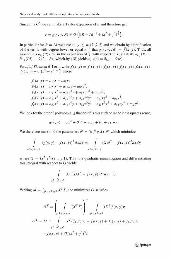
Since h is C5 we can make a Taylor expansion of h and therefore get

z = g(x, y, R) + O(||R − I d||5 + (x2 + y2)

52

).

In particular for R = I d we have (x, y, z) = (x, y, z) and we obtain by identificationof the terms with degree lower or equal to 4 that g(x, y, I d) = f (x, y). Thus, allmonomials ai j (R)xi y j in the expansion of f with respect to x, y satisfy ai, j (R) =ai, j (I d) + O(I − R), which by (18) yields ai, j (r) = ai, j + O(r).

Proof of Theorem 6 Let us write f (x, y) = f1(x, y)+ f2(x, y)+ f3(x, y)+ f4(x, y)+f5(x, y) + o(|x2 + y2|5/2) where

f1(x, y) = a10x + a01 y,

f2(x, y) = a20x2 + a11xy + a02 y2,

f3(x, y) = a30x3 + a21x2 y + a12xy2 + a03 y3,

f4(x, y) = a40x4 + a31x3 y + a22x2 y2 + a13xy3 + a04 y4,

f5(x, y) = a50x5 + a41x4 y + a32x3 y2 + a23x2 y3 + a14xy4 + a05 y5.

We look for the order 2 polynomial g that best fits this surface in the least squares sense,

g(x, y) = αx2 + βy2 + γ xy + δx + εy + θ.

We therefore must find the parameters Θ = (α β γ δ ε θ) which minimize

∫

x2+y2<r2

(g(x, y) − f (x, y))2 dxdy =∫

x2+y2<r2

(XΘT − f (x, y))2dxdy

where X = (x2 y2 xy x y 1

). This is a quadratic minimization and differentiating

this integral with respect to Θ yields

∫

x2+y2<r2

X T (XΘT − f (x, y))dxdy = 0.

Writing M = ∫x2+y2<r2 X T X, the minimizer Θ satisfies

ΘT =⎛

⎜⎝

∫

x2+y2<r2

(X T X)

⎞

⎟⎠

−1∫

x2+y2<r2

(X T f (x, y));

ΘT = M−1∫

x2+y2<r2

X T ( f1(x, y) + f2(x, y) + f3(x, y) + f4(x, y)

+ f5(x, y) + O((x2 + y2)3);

123

J. Digne, J.-M. Morel

where X T X =

⎛

⎜⎜⎜⎜⎜⎜⎝

x4 x2 y2 x3 y x3 x2 y x2

x2 y2 y4 xy3 xy2 y3 y2

x3 y xy3 x2 y2 x2 y xy2 xyx3 xy2 x2 y x2 xy x

x2 y y3 xy2 xy y2 yx2 y2 xy x y 1

⎞

⎟⎟⎟⎟⎟⎟⎠

.

When integrating on the disk, most terms vanish and we get

M = πr4

4

⎛

⎜⎜⎜⎜⎜⎜⎜⎜⎜⎝

r2

2r2

6 0 0 0 1

r2

6r2

2 0 0 0 1

0 0 r2

6 0 0 00 0 0 1 0 00 0 0 0 1 01 1 0 0 0 4

r2

⎞

⎟⎟⎟⎟⎟⎟⎟⎟⎟⎠

; M−1 = 4

πr4

⎛

⎜⎜⎜⎜⎜⎜⎜⎜⎝

92r2

32r2 0 0 0 − 3

2

32r2

92r2 0 0 0 − 3

2

0 0 6r2 0 0 0

0 0 0 1 0 00 0 0 0 1 0

− 32 − 3

2 0 0 0 r2

⎞

⎟⎟⎟⎟⎟⎟⎟⎟⎠

.

Therefore

ΘT = M−1∫

x2+y2<r2

X T f1(x, y) + M−1∫

x2+y2<r2

X T f2(x, y)

+M−1∫

x2+y2<r2

X T f3(x, y) + M−1∫

x2+y2<r2

X T f4(x, y)

+M−1∫

x2+y2<r2

X T f5(x, y) + M−1∫

x2+y2<r2

X T O((x2 + y2)4),

with∫

x2+y2<r2

X T f1(x, y) = πr4

4

⎛

⎜⎜⎜⎜⎝

000

a10a01

⎞

⎟⎟⎟⎟⎠

;

∫

x2+y2<r2

X T f2(x, y) = πr4

4

⎛

⎜⎜⎜⎜⎜⎜⎜⎜⎝

r2

6 (3a20 + a02)

r2

6 (a20 + 3a02)

r2

6 a11

00

a20 + a02

⎞

⎟⎟⎟⎟⎟⎟⎟⎟⎠

;

123

Numerical analysis of differential operators on raw point clouds

∫

x2+y2<r2

X T f3(x, y) = πr4

4

⎛

⎜⎜⎜⎜⎜⎜⎜⎝

000

r2

6 (3a30 + a12)

r2

6 (a21 + 3a03)

0

⎞

⎟⎟⎟⎟⎟⎟⎟⎠

;

∫

x2+y2<r2

X T f4(x, y) = πr4

4

⎛

⎜⎜⎜⎜⎜⎜⎜⎜⎜⎜⎝

r4

16 (5a40 + a22 + a04)

r4

16 (a40 + a22 + 5a04)

r4

16 (a31 + a13)

00

r2

6 (3a40 + a22 + 3a04)

⎞

⎟⎟⎟⎟⎟⎟⎟⎟⎟⎟⎠

;

∫

x2+y2<r2

X T ( f5(x, y)) = πr4

4

⎛

⎜⎜⎜⎜⎜⎜⎜⎜⎝

000

r4

16 (5a50 + a32 + a14)

r4

16 (a41 + a23 + 5a05)

0

⎞

⎟⎟⎟⎟⎟⎟⎟⎟⎠

;

∫

x2+y2<r2

X T (x2 + y2)3 = πr4

4

⎛

⎜⎜⎜⎜⎜⎜⎜⎜⎜⎝

2r6

5

2r6

5

000r4

2

⎞

⎟⎟⎟⎟⎟⎟⎟⎟⎟⎠

.

Multiplying all of these results by the matrix M−1, we get

M−1∫

x2+y2<r2

X T f1(x, y) =

⎛

⎜⎜⎜⎜⎜⎜⎝

000

a10a010

⎞

⎟⎟⎟⎟⎟⎟⎠

; (20)

M−1∫

x2+y2<r2

X T f2(x, y) =

⎛

⎜⎜⎜⎜⎜⎜⎝

a20a02a11000

⎞

⎟⎟⎟⎟⎟⎟⎠

; (21)

123

J. Digne, J.-M. Morel

M−1∫

x2+y2<r2

X T ( f3(x, y)) =

⎛

⎜⎜⎜⎜⎜⎜⎜⎜⎝

000

r2

6 (3a30 + a12)

r2

6 (a21 + 3a03)

0

⎞

⎟⎟⎟⎟⎟⎟⎟⎟⎠

; (22)

M−1∫

x2+y2<r2

X T ( f4(x, y)) =

⎛

⎜⎜⎜⎜⎜⎜⎜⎜⎜⎜⎝

r2

8 (6a40 + a22)

r2

8 (a22 + 6a04)

3r2

8 (a31 + a13)

00

− r4

48 (3a40 + a22 + 3a04)

⎞

⎟⎟⎟⎟⎟⎟⎟⎟⎟⎟⎠

; (23)

M−1∫

x2+y2<r2

X T ( f5(x, y)) =

⎛

⎜⎜⎜⎜⎜⎜⎜⎜⎝

000

r4

16 (5a50 + a32 + a14)

r4

16 (a41 + a23 + 5a05)

0

⎞

⎟⎟⎟⎟⎟⎟⎟⎟⎠

; (24)

M−1∫

x2+y2<r2

X T (x2 + y2)3 =

⎛

⎜⎜⎜⎜⎜⎜⎜⎜⎜⎝

33r4

20

33r4

20

000

− 7r6

10

⎞

⎟⎟⎟⎟⎟⎟⎟⎟⎟⎠

, (25)

and combining (20), (21), (22), (23), (24) and (25) we finally obtain the parameter Θ

ΘT =

⎛

⎜⎜⎜⎜⎜⎜⎜⎜⎜⎜⎜⎜⎜⎝

a20 + r2

8 (a22 + 6a40) + O(r4)

a02 + r2

8 (a22 + 6a04) + O(r4)

a11 + 3r2

8 (a13 + a31) + O(r4)

a10 + r2

6 (a12 + 3a30) + r4

16 (5a50 + a32 + a14) + O(r5)

a01 + r2

6 (3a03 + a21) + r4

16 (a41 + a23 + 5a05) + O(r5)

− r4

48 (3a04 + a22 + 3a40) + O(r6)

⎞

⎟⎟⎟⎟⎟⎟⎟⎟⎟⎟⎟⎟⎟⎠

123

Numerical analysis of differential operators on raw point clouds

so that the MLS2 projection satisfies g(0, 0) = − r4

48 (3a04 + a22 + 3a40) + O(r6).

Finally Lemma 4 permits to replace g(0, 0) = − r4

48 (3a04 + a22 + 3a40) + O(r6) by

−(

r4

48(3a04 + a22 + 3a40) + O(r6)

)

(1 + O(r))

= − r4

48(3a04 + a22 + 3a40) + O(r5).

��We shall now analyze experimentally those results.

6 Numerical experiments

This section performs numerical comparative experiments with the most significantalgorithms described in the previous sections. A simulated randomly sampled spherewill play the role of numerical pattern. In particular we evaluate the mean curvaturesgiven on the sphere by MLS1 projection and MLS2 projection followed by polynomialregression. We also compute the curvature estimated by the method described in [7]and by the surface variation of [40]. The results are compared by giving the meanestimated curvature and its standard variation. The input data is a randomly sampledsphere with radius 2 corrupted with added centered Gaussian noise of variance 0.1.

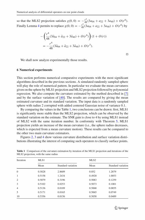
By comparing the values in the Table 1, two conclusions can be drawn: first, MLS1is significantly more stable than the MLS2 projection, which can be observed by thestandard variation on the estimate. The SNR gain is close to 4 by using MLS1 insteadof MLS2 with the same iteration number. In conformity with Theorem 5, MLS1projection yields an increase of the mean curvature (i.e., the sphere radius decreases,which is expected from a mean curvature motion). These results can be compared tothe other two main curvature estimators.

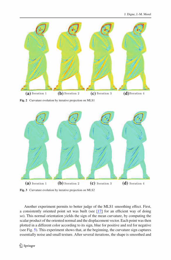
Figures 2, 3 and 4 show various curvature distribution and surface variation distri-butions illustrating the interest of computing such operators to classify surface points.

Table 1 Comparison of the curvature estimation by iteration of the MLS1 projection and iterations of theMLS2 projection, with the same radius

Iteration MLS1 MLS2

Mean Standard variation Mean Standard variation

0 0.5828 2.8609 0.052 1.2879

1 0.5158 1.2434 0.4920 1.0053

2 0.5079 0.3196 0.5083 0.1259

3 0.5102 0.0253 0.5073 0.1001

4 0.5136 0.0189 0.5068 0.0855

5 0.5171 0.0165 0.5065 0.0749

10 0.5356 0.0156 0.5058 0.0489

123

J. Digne, J.-M. Morel

(a) (b) (c) (d)Fig. 2 Curvature evolution by iterative projection on MLS1

(a) (b) (c) (d)Fig. 3 Curvature evolution by iterative projection on MLS2

Another experiment permits to better judge of the MLS1 smoothing effect. First,a consistently oriented point set was built (see [17] for an efficient way of doingso). This normal orientation yields the sign of the mean curvature, by computing thescalar product of the oriented normal and the displacement vector. Each point was thenplotted in a different color according to its sign, blue for positive and red for negative(see Fig. 5). This experiment shows that, at the beginning, the curvature sign capturesessentially noise and small texture. After several iterations, the shape is smoothed and

123

Numerical analysis of differential operators on raw point clouds

Fig. 4 Other curvatureestimates

(a) (b)

Fig. 5 Evolution of the motion direction with projection iterations

the sign captures the geometry of the shape (large scale variations), which is the mainadvantage of the scale space strategy.

To compare the techniques analyzed theoretically in the previous sections, we finallyused randomly sampled shapes with added Gaussian noise. We compared betweencomputing the covariance of the points projected onto the local tangent plane, asdescribed in Sect. 4.1 (called 2dcov1 in the remainder of this section); computing thecovariance of the unit normals projected on the regression plane, as described in Sect.4.2 (called 2dcov2 in the remainder of this section); computing the covariance of theunit normals, as described in Sect. 4.3 (called 3dcov in the remainder of this section);and finally MLS2. The 2dcov1 method was immediately discarded, because it does

123

J. Digne, J.-M. Morel

not yield a separate estimate of the principal curvatures. We therefore only comparedthe other three methods.

To do so the estimators were compared on three kinds of noisy surfaces: a sphere,a cylinder and a torus with added gaussian noise in the normal direction. The goalwas not to compute the actual curvatures of the noiseless surface, but to contrast therobustness of these local surface geometric indicators which replace the infinitesimalcurvatures. The asymptotic Theorems 1 2, 3, and 4 show that the considered intrinsiclocal integral estimators retain the same structure properties as the real differentialoperators. Thus, our goal is to select among them the ones that have the best SNR. Onthe other hand the SNR depends of course of the radius on which these operators arecomputed. The smaller the radius, the more faithful these operators will be to localcurvature operators. Thus, all things being equal, it is better to compute them withsmall radii. But of course the SNR decreases with the radius. Thus, to compare thepower of these local integral operators, the best way is to compare the SNR’s withfixed radius or, equivalently, to compare their radii for fixed SNR. Yet there are twoparameters for MLS1: the radius r and the number of iterations N . But both parameterscan be an equivalent radius. Indeed, applying N iterations of MLS1 with radius r isroughly equivalent to applying one iteration of the scale space with radius rq = √

Nr(this equivalence is drawn by analogy with iterated linear filters). The numerical tablesgive the equivalent radius value for MLS1.

A sphere and a cylinder were used because they have constant curvatures on thewhole surface. We also considered a torus, because one can compute the operatorson invariant circles of the torus, where curvatures should be constant in absence ofnoise. As just explained, the radii were set so that each method gives the same standardvariation for the estimate of the same curvature.

One should first notice that 3dcov and 2dcov2 give very similar results. This is notsurprising since both methods rely on the normal covariance matrix (actually, eventheir asymptotic behavior is the same, see Theorems 2 and 3).

Tables 2, 3 and 4 show the results after this calibration of the experiment by thestandard deviation. Two conclusions can be drawn from these experiments. First, theradii needed for getting a small standard variation are slightly larger for 2dcov2, 3dcovand significantly larger for MLS2, than for MLS1. This has the direct consequence

Table 2 Comparison of the mean curvature estimates on a noisy sphere with radius 2 and noise variance0.05

Parameters Stdev SNR

MLS1 N = 5, r = 0.14, req = 0.31 0.026 20.0

2dcov2 r = 0.3 0.027 17.6

3dcov r = 0.3 0.027 17.6

MLS2 r = 0.6 0.029 15.6

Calibration is done by setting the parameters so that the standard deviation is similar. The parameters arethe neighborhood radius r and the number of iterations N in the case of MLS1. The best SNR is obtainedwith MLS1, which is also the fastest method. But 2dcov2 and 3dcov have similar performance, while MLS2is clearly worse (its radius doubles for a lower SNR)

123

Numerical analysis of differential operators on raw point clouds

Table 3 Comparison of the mean curvature estimates on a noisy cylinder with radius 1 and noise variance0.05

Parameters Stdev SNR

MLS1 N = 5, r = 0.16, req = 0.36 0.040 16.2

2dcov2 r = 0.37 0.032 16.9

3dcov r = 0.3 0.031 16.9

MLS2 r = 0.6 0.036 13.2

The radius r or equivalent radius req are set so that the standard deviation becomes similar. The conclusionsare the same as in Table 2

Table 4 Comparison of the mean curvature estimates for an invariant circle of a noisy torus with radii 2and 0.5 and noise variance 0.02

Parameters Stdev SNR

MLS1 N = 4, r = 0.07, req = 0.14 0.032 34.2

2dcov2 r = 0.15 0.031 31.8

3dcov r = 0.15 0.031 31.8

MLS2 r = 0.32 0.030 1.2

Here again, the filtering radii were chosen so that the standard deviation becomes similar, and the SNR’sand radii can therefore be compared. Here again MLS1 wins by a small margin on 2dcov2 and 3dcov, andby a large margin over MLS2

that computation times are significantly higher for those methods than for MLS1: itis indeed faster to iterate a method working on a small neighborhood than to do asingle iteration of a method requiring a large neighborhood. Nevertheless, MLS1 onlyprovides us with an estimated equivalent to the mean curvature but does not give anestimated equivalent of the principal curvatures nor of the principal directions. As amatter of fact only MLS2 provides this information: 2dcov2 and 3dcov only providethe principal directions and the squared principal curvatures. Yet we saw that in orderfor MLS2 to be resilient to noise a large neighborhood must be used which leads tohuge computation times.

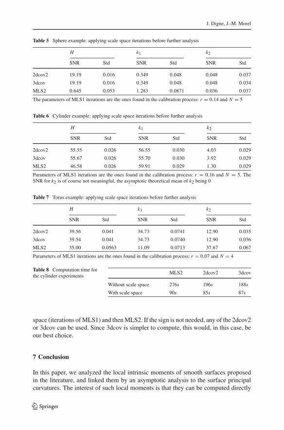
Since we proved that MLS1 is consistent with an intrinsic heat equation, it plays thespecial role among the considered operators of simulating a scale space semigroup.Using the scale space paradigm, it can be used previously to the computation of otherdifferential operators. We did again the same computations using the MLS1 iterations(scale space) before applying the more complex methods. We used the same numberof iterations for MSLS1 as found in Tables 2, 3 and 4 and performed the next analysisusing the same radius. The new tables (Tables 5, 6, 7) show how the scale space makesit possible to compute reliably the same moments with a smaller processing radius.Computation times being the bottleneck of all numerical methods, we compare onTable 8 the computation times obtained on the cylinder when applying all the methods(with the same parameters as in Tables 3 and 6: it is straightforward that applying theMLS1 iterations is a much better strategy to get manageable numerical experiments.

These numerical experiments confirm that the only way to recover a robust signedintegro-differential operator, equivalent to the mean curvature, is to apply the scale

123

J. Digne, J.-M. Morel

Table 5 Sphere example: applying scale space iterations before further analysis

H k1 k2

SNR Std SNR Std SNR Std

2dcov2 19.19 0.016 0.349 0.048 0.048 0.037

3dcov 19.19 0.016 0.349 0.048 0.048 0.034

MLS2 0.645 0.053 1.283 0.0871 0.036 0.037

The parameters of MLS1 iterations are the ones found in the calibration process: r = 0.14 and N = 5

Table 6 Cylinder example: applying scale space iterations before further analysis

H k1 k2

SNR Std SNR Std SNR Std

2dcov2 55.55 0.026 56.55 0.030 4.03 0.029

3dcov 55.67 0.026 55.70 0.030 3.92 0.029

MLS2 46.58 0.026 59.91 0.029 1.30 0.029

Parameters of MLS1 iterations are the ones found in the calibration process: r = 0.16 and N = 5. TheSNR for k2 is of course not meaningful, the asymptotic theoretical mean of k2 being 0

Table 7 Torus example: applying scale space iterations before further analysis

H k1 k2

SNR Std SNR Std SNR Std

2dcov2 39.56 0.041 34.73 0.0741 12.90 0.035

3dcov 39.54 0.041 34.73 0.0740 12.90 0.036

MLS2 35.00 0.0563 11.09 0.0713 37.67 0.067

Parameters of MLS1 iterations are the ones found in the calibration process: r = 0.07 and N = 4

Table 8 Computation time forthe cylinder experiments

MLS2 2dcov2 3dcov

Without scale space 276s 196s 188s

With scale space 90s 85s 87s

space (iterations of MLS1) and then MLS2. If the sign is not needed, any of the 2dcov2or 3dcov can be used. Since 3dcov is simpler to compute, this would, in this case, beour best choice.

7 Conclusion

In this paper, we analyzed the local intrinsic moments of smooth surfaces proposedin the literature, and linked them by an asymptotic analysis to the surface principalcurvatures. The interest of such local moments is that they can be computed directly

123

Numerical analysis of differential operators on raw point clouds

on raw point clouds and therefore allow for a direct numerical analysis of such rawdata. We showed that these clever methods only recover the equivalent of squaredprincipal curvatures, and loose their signs.

The alternative method to compute curvatures on the surface is the order 2 regressionMLS2. An asymptotic analysis of MLS2 confirms that is is accurate with order 4 andalso uncovers a new intrinsic fourth order partial differential operator arising naturallyfrom this order 2 regression.

Finally the analysis of the MLS1 projection (recalled from [17]) yields a mean cur-vature motion. Once iterated this scale space operator, proven very robust to irregularsampling, gives an alternative way to compute curvatures by combining scale spaceand MLS2. Numerical experiments herewith have shown this to be the most reliablemethod, in agreement with the scale space methodology already established in imageanalysis.

Acknowledgments The authors acknowledge support by the E.R.C. advanced grant “Twelve labours”.

References

1. Alexa, M., Adamson, A.: Interpolatory point set surfaces convexity and hermite data. ACM Trans.Graph. 28, 20:1–20:10 (2009)

2. Alexa, M., Behr, J., Cohen-Or, D., Fleishman, S., Levin, D., Silva, C.T.: Point set surfaces. In: Pro-ceedings of the Conference on Vis ’01, pp. 21–28. IEEE Computer Society, Washington, DC (2001)

3. Alexa, M., Behr, J., Cohen-Or, D., Fleishman, S., Levin, D., Silva, C.T.: Computing and renderingpoint set surfaces. IEEE TVCG 9(1), 3–15 (2003)

4. Alliez, P., Cohen-Steiner, D., Tong, Y., Desbrun, M.: Voronoi-based variational reconstruction ofunoriented point sets. In: Proceedings of the SGP ’07, pp. 39–48. Eurographics, Switzerland (2007)

5. Amenta, N., Kil, Y.J.: Defining point-set surfaces. In: Proceedings of the SIGGRAPH ’04: ACMSIGGRAPH 2004 Papers, pp. 264–270. ACM Press, USA (2004)

6. Belkin, M., Sun, J., Wang, Y.: Constructing laplace operator from point clouds in rd. In: Proceedingsof the SODA ’09, pp. 1031–1040. SIAM, USA (2009)

7. Berkmann, J., Caelli, T.: Computation of surface geometry and segmentation using covariance tech-niques. IEEE PAMI 16(11), 1114–1116 (1994)

8. Buades, A., Coll, B., Morel, J.M.: Neighborhood filters and pdes. Numer. Math. 105(1), 1–34 (2006)9. Carr, J.C., Beatson, R.K., Cherrie, J.B., Mitchell, T.J., Fright, W.R., McCallum, B.C., Evans, T.R.:

Reconstruction and representation of 3d objects with radial basis functions. In: SIGGRAPH 01, Pro-ceedings of the 28th annual conference on Computer Graphics and Interactive Technics, pp. 67–76(2001)

10. Cazals, F., Pouget, M.: Estimating differential quantities using polynomial fitting of osculating jets.In: Proceedings of the SGP ’03, pp. 177–187. Eurographics, Switzerland (2003)

11. Cazals, F., Pouget, M.: Topology driven algorithms for ridge extraction on meshes. Tech. Rep. INRIA(2005)

12. Clarenz, U., Griebel, M., Rumpf, M., Schweitzer, M.A., Telea, A.: Feature sensitive multiscale editingon surfaces. Vis. Comput. 20, 329–343 (2004)

13. Clarenz, U., Rumpf, M., Telea, A.: Robust feature detection and local classification for surfaces basedon moment analysis. IEEE Trans. Vis. Comput. Graph. 10, 516–524 (2004)

14. Cohen-Steiner, D., Morvan, J.M.: Restricted delaunay triangulations and normal cycle. In: Proceedingsof the SCG ’03, pp. 312–321. ACM, USA (2003)

15. Curless, B., Levoy, M.: A volumetric method for building complex models from range images. In:Proceedings of the SIGGRAPH ’96, pp. 303–312. ACM Press, USA (1996)

16. Desbrun, M., Meyer, M., Schroder, P., Barr, A.H.: Implicit fairing of irregular meshes using diffusionand curvature flow. In: Proceedings of the SIGGRAPH ’99, pp. 317–324. ACM Press/Addison-WesleyPublishing Co., USA (1999)

123

J. Digne, J.-M. Morel

17. Digne, J., Morel, J.M., Mehdi-Souzani, C., Lartigue, C.: Scale space meshing of raw data point sets.Comput. Graph. Forum. 30(6):1630–1642 (2011)

18. Fleishman, S., Cohen-Or, D., Silva, C.T.: Robust moving least-squares fitting with sharp features. ACMTrans. Graph. 24(3), 544–552 (2005)

19. Gelfand, N., Mitra, N.J., Guibas, L.J., Pottmann, H.: Robust global registration. In: Proceedings ofthe Third Eurographics Symposium on Geometry Processing. Eurographics Association, Switzerland(2005)

20. Gross, M., Hubeli, A.: Eigenmeshes Technical Report. ETH Zurich, Switzerland (2000)21. Guennebaud, G., Gross, M.: Algebraic point set surfaces. ACM Trans. Graph. 26(3), (2007)22. Hoppe, H., DeRose, T., Duchamp, T., McDonald, J., Stuetzle, W.: Surface reconstruction from unor-

ganized points. In: Proceedings of the SIGGRAPH ’92, pp. 71–78. ACM Press, USA (1992)23. Hubeli, A., Gross, M.: Multiresolution feature extraction for unstructured meshes. In: Proceedings of

the Conference on Visualization ’01, pp. 287–294. IEEE Computer Society, Washington, DC (2001)24. Hulin, D., Troyanov, M.: Mean curvature and asymptotic volume of small balls. Am. Math. Mon.

110(10), 947–950 (2003)25. Kalogerakis, E., Simari, P., Nowrouzezahrai, D., Singh, K.: Robust statistical estimation of curvature

on discretized surfaces. In: Proceedings of the SGP ’07, pp. 13–22. Eurographics, Switzerland (2007)26. Karni, Z., Gotsman, C.: Spectral compression of mesh geometry. In: Proceedings of the 27th Annual

Conference on Computer Graphics and Interactive Techniques (SIGGRAPH ’00), pp. 279–286. ACMPress/Addison-Wesley Publishing Co., USA (2000)

27. Kazhdan, M.: Reconstruction of solid models from oriented point sets. In: Proceedings of the SGP’05, p. 73. Eurographics Association, Switzerland (2005)

28. Kazhdan, M., Bolitho, M., Hoppe, H.: Poisson surface reconstruction. In: Proceedings of the SGP ’06,pp. 61–70. Eurographics, Switzerland (2006)

29. Kobbelt, L.P., Botsch, M., Schwanecke, U., Seidel, H.P.: Feature sensitive surface extraction fromvolume data. In: Proceedings of the SIGGRAPH ’01, pp. 57–66. ACM, USA (2001)

30. Lancaster, P., Salkauskas, K.: Surfaces generated by moving least squares methods. Math. Comput.37(155), 141–158 (1981)

31. Levin, D.: The approximation power of moving least-squares. Math. Comput. 67(224), 1517–1531(1998)

32. Levin, D.: Mesh-independent surface interpolation. In: Brunnett, G., Hamann, B., Müller, H., Linsen, L.(eds.) Geometric Modeling for Scientific Visualization, pp. 37–49. Springer, New York (2003)

33. Liang, P., Todhunter, J.S.: Representation and recognition of surface shapes in range images: a differ-ential geometry approach. Comput. Vision Graph. Image Process. 52(1), 78–109 (1990)

34. Lipman, Y., Cohen-Or, D., Levin, D.: Data-dependent mls for faithful surface approximation. In:Proceedings of the SGP ’07, pp. 59–67. Eurographics, Switzerland (2007)

35. Lorensen, W.E., Cline, H.E.: Marching cubes: a high resolution 3d surface construction algorithm. In:Proceedings of the SIGGRAPH ’87, pp. 163–169. ACM Press, USA (1987)

36. Magid, E., Soldea, O., Rivlin, E.: A comparison of gaussian and mean curvature estimation methodson triangular meshes of range image data. CVIU 107(3), 139–159 (2007)

37. Mérigot, Q., Ovsjanikov, M., Guibas, L.J.: Robust Voronoi-based curvature and feature estimation. In:Proceedings of the SIAM/ACM Joint Conference on Geometric and Physical Modeling. San Francisco,USA (2009)

38. Meyer, M., Desbrun, M., Schröder, P., Barr, A.: Discrete differential geometry operators for triangulated2-manifolds. In: Proceedings of the International Workshop on Visualization and Mathematics (2002)

39. Oztireli, A.C., Guennebaud, G., Gross, M.: Feature preserving point set surfaces based on non-linearkernel regression. CGF 28(9), 493–501 ((2009))

40. Pauly, M., Gross, M., Kobbelt, L.P.: Efficient simplification of point-sampled surfaces. In: Proceedingsof the VIS ’02, pp. 163–170. IEEE, USA (2002)

41. Pauly, M., Kobbelt, L.P., Gross, M.: Point-based multiscale surface representation. ACM Trans. Graph.25(2), 177–193 (2006)

42. Pottmann, H., Wallner, J., Huang, Q.X., Yang, Y.L.: Integral invariants for robust geometry processing.CAGD 26(1), 37–60 (2009)

43. Pottmann, H., Wallner, J., Yang, Y.L., Lai, Y.K., Hu, S.M.: Principal curvatures from the integralinvariant viewpoint. CAGD 24(8–9), 428–442 (2007)

44. Rusinkiewicz, S.: Estimating curvatures and their derivatives on triangle meshes. In: Proceedings ofthe 3DPVT ’04, pp. 486–493. IEEE, USA (2004)

123

Numerical analysis of differential operators on raw point clouds

45. Tang, X.: A sampling framework for accurate curvature estimation in discrete surfaces. IEEE TVCG11(5), 573–583 (2005)

46. Taubin, G.: Estimating the tensor of curvature of a surface from a polyhedral approximation. In:Proceedings of the ICCV ’95, p. 902. IEEE, USA (1995)

47. Taubin, G.: A signal processing approach to fair surface design. In: Proceedings of the SIGGRAPH’95, pp. 351–358. ACM Press, USA (1995)

48. Theisel, H., Rossl, C., Zayer, R., Seidel, H.P.: Normal based estimation of the curvature tensor fortriangular meshes. In: Proceedings of the PG’ 04, pp. 288–297. IEEE, USA (2004)

49. Tong, W.S., Tang, C.K.: Robust estimation of adaptive tensors of curvature by tensor voting. IEEEPAMI 27(3), 434–449 (2005)

50. Unnikrishnan, R., Hebert, M.: Multi-scale interest regions from unorganized point clouds. In: Proceed-ings of the Workshop on Search in 3D (S3D), IEEE CVPR, New York (2008)

51. Yang, P., Qian, X.: Direct computing of surface curvatures for point-set surfaces. In: Proceedings ofthe PBG 07 (2007)

52. Yang, Y.L., Lai, Y.K., Hu, S.M., Pottmann, H.: Robust principal curvatures on multiple scales. In:Proceedings of the SGP ’06, pp. 223–226. Eurographics, Aire-la-Ville (2006)

123