Computational Statistics and Data Analysis 52 (2008) 4325–4345www.elsevier.com/locate/csda

Notes on estimation of proportion ratio under a non-compliancerandomized trial with missing outcomes

Kung-Jong Luia,∗, William G. Cumberlandb

a Department of Mathematics and Statistics, San Diego State University, San Diego, CA 92182-7720, USAb Department of Biostatistics, University of California, Los Angeles, CA 90265, USA

Received 23 October 2006; received in revised form 13 February 2008; accepted 13 February 2008Available online 17 February 2008

Abstract

When measuring the efficacy of an experimental treatment in dichotomous data, we often employ the proportion ratio (PR)of a positive response (or an adverse event) between the experimental and standard treatments. In this paper, we consider a non-compliance randomized clinical trial with outcomes missing at random (MAR). We derive the maximum likelihood estimator(MLE) for the PR under the model in which missingness depends only on assigned treatments, and the model in which missingnessdepends on both assigned and received treatments. We develop three asymptotic interval estimators for the PR under the lattersituation. We apply Monte Carlo simulation to evaluate and compare the performance of these estimators in a variety of situations.We note that the point estimator assuming outcomes missing completely at random (MCAR) can be subject to a serious bias undervarious models with MAR, and the point estimators developed here may consistently perform reasonably well when the number ofpatients per assigned treatment is large. We find that the interval estimator using Wald’s statistic tends to lose accuracy with respectto the coverage probability, while the interval estimator using the logarithmic transformation tends to lose precision with respect tothe average length. We also find that an ad hoc combination of the previous two interval estimators can consistently perform wellin many situations. Finally, we use data taken from a multiple risk factor intervention trial for reducing mortality of coronary heartdisease to illustrate the bias of the point estimator for MCAR and the use of these point and interval estimators for the PR underthe assumed MAR.c© 2008 Elsevier B.V. All rights reserved.

1. Introduction

When measuring the efficacy of an experimental treatment, we often consider the use of the proportion ratio (PR)of a positive response (or an adverse event) between the experimental and standard treatments (Lui, 2006a). When thePR represents the ratio of probabilities of an adverse event, the PR is also called the relative risk or risk ratio (RR), andis one of the most frequently used indices to measure the strength of association between a risk factor and a disease inetiological studies (Fleiss, 1981; Lui, 2004). When RR < 1, the relative difference (Sheps, 1958, 1959; Fleiss, 1981;Lui, 2004) or the relative risk reduction is simply equal to 1−RR (Fleiss, 1981; Lui, 2004). Thus, the results presentedhere are applicable if the latter index is of our interest.

∗ Corresponding author. Tel.: +1 619 594 6191; fax: +1 619 594 6746.E-mail address: kjl@rohan.sdsu.edu (K.-J. Lui).

0167-9473/$ - see front matter c© 2008 Elsevier B.V. All rights reserved.doi:10.1016/j.csda.2008.02.011

4326 K.-J. Lui, W.G. Cumberland / Computational Statistics and Data Analysis 52 (2008) 4325–4345

Non-compliance can occur in a randomized clinical trial (RCT) due to ethical or other reasons. When a patientassigned to an experimental treatment has serious reactions (or personal concerns), the patient should be given theoption to switch to the best standard treatment (Zelen, 1979, 1986, 1990). Also, we may come across a treatmentfor which we cannot apply the traditional RCT to study its effect. For example, it would be unethical to randomlyassign high-risk patients to receive either a flu vaccine or a placebo in a flu shot trial. To alleviate this concern,the randomized encouragement design (RED), in which each patient is randomly assigned to either the interventiongroup in which the patient receives an encouragement for using an experimental treatment or to the control groupin which the patient receives no encouragement, has recently received a lot of attention (Multiple Risk FactorIntervention, 1982; Matsui, 2005; McDonald et al., 1992; Zhou and Li, 2006). The basic idea of RED is to increasethe number of patients to receive the experimental treatment through encouragement in the intervention groupwithout affecting the selection of a treatment for patients assigned to the control group in a RCT. Thus, if thereis a difference in the response rates among patients between the intervention and control groups, we may attributethis to the effect of the experimental treatment. When employing the RED, however, we frequently encounter twoimportant analytic issues: a high rate of non-compliance and a non-negligible percentage of missing outcomes (Zhouand Li, 2006). The former is due to the fact that patients may receive the experimental or the standard treatmentregardless of whether he/she receives an encouragement. The latter can occur because of patients’ refusal or lossto follow-up (Frangakis and Rubin, 1999) during a long period RCT. Since non-compliance and missing outcomesdo not generally occur at random, simply analyzing data as treated or arbitrarily excluding patients with missingoutcomes from the data analysis may lead us to misleading conclusions. Frangakis and Rubin (1999) proposeda compound exclusion restriction model and discussed estimation of the intention-to-treat effect measured by therisk difference (RD) in the presence of missing outcomes. However, they focused their consideration on the simplecompliance trial (Sommer and Zeger, 1991; Lui, 2007), in which only patients assigned to the experimental treatmentcould be allowed to switch to the other treatment. Zhou and Li (2006) considered a non-compliance RCT withmissing outcomes, in which patients assigned to both treatments were allowed to switch to the other treatment,and focused their discussion on estimation of the RD under the compound exclusion restriction model as well.The application of Zhou’s and Li’s methods involved intensive iterative numerical procedures. Because of thecomplexity in their estimation procedures, no variances of Zhou’s and Li’s estimators in closed forms were given.Other papers addressing the estimation of the treatment effect under a non-compliance RCT with missing data whenthe outcomes are continuous have appeared elsewhere (Yau and Little, 2001; Barnard et al., 2003). None of thesediscussed estimation of PR under a non-compliance RCT with missing outcomes. Because the data structure for thenon-compliance RCT is essentially parallel to that of the pre-randomized design (Zelen, 1979, 1986, 1990; Anbar,1983; Sommer and Zeger, 1991; Brunner and Neumann, 1985; Bernhard and Compagnone, 1989; Lui and Lin, 2003;Matts and McHugh, 1987, 1993; McHugh, 1984), the results and findings presented here are applicable to the latteras well.

In this paper, we focus the discussion on estimation of the PR under a non-compliance RCT with outcomes missingat random (MAR). Using an approach similar to that proposed elsewhere (Brunner and Neumann, 1985; Bernhardand Compagnone, 1989), we derive in Sections 2.1–2.3 the maximum likelihood estimator (MLE) for the PR undervarious assumptions, including the model in which there is no missingness, the model in which missingness dependson only assigned treatments, and the model in which missingness depends on both assigned and received treatments.In Section 2.4, we develop three asymptotic interval estimators in closed form for the PR under the model in whichmissingness depends on assigned and received treatments. We use Monte Carlo simulation to study the performanceof point estimators developed in Section 3.1 and the performance of the three asymptotic interval estimators inSection 3.2. We note that the point estimator for missing completely at random (MCAR) can be subject to a seriousbias under various models with MAR. By contrast, we note that the point estimators developed in this paper canperform well when the number of patients per assigned treatment is large. Further, we find that the asymptotic intervalestimator using Wald’s statistic tends to lose accuracy with respect to the coverage probability, while the intervalestimator using the logarithmic transformation (Katz et al., 1978; Fleiss, 1981; Lui, 2002) tends to lose precisionwith respect to the average length. Finally, we note that an interval estimator, formed by an ad hoc combination ofthe previous two estimators, can perform well in almost all situations considered here. We apply the data taken froma multiple risk factor intervention trial for reducing the mortality of coronary heart disease (Multiple Risk FactorIntervention, 1982) in Section 3.3 to illustrate the bias of the point estimator for MCAR, and the use of the abovepoint and interval estimators under the assumed MAR.

K.-J. Lui, W.G. Cumberland / Computational Statistics and Data Analysis 52 (2008) 4325–4345 4327

2. Notations and methods

Consider comparing an experimental treatment with a standard treatment under a RCT, in which each patient can bepotentially assigned to either of these two treatments G (=1 for experimental, and =0 for standard). Following Angristet al. (1996), we define for each patient the function D(G) as the status of his/her received treatment, where D(G) = 1if the patient assigned to treatment G actually receives the experimental treatment, and D(G) = 0 otherwise. Thus, wecan divide our population into four subpopulations. These include compliers (D(1) = 1 and D(0) = 0), never-takers(D(1) = D(0) = 0), always-takers (D(1) = D(0) = 1), and defiers (D(1) = 0 and D(0) = 1). As commonlyassumed for a RCT with non-compliance (Li and Frangakis, 2005; Zhou and Li, 2006), we assume monotonicity(D(1) ≥ D(0)) for all patients (i.e., no defiers) in the following discussion. Brunner and Neumann (1985) contendedthat a patient who refused a proffered treatment should only stay in the study if he/she preferred the other treatment.In practice, a patient who is a defier may not even provide his/her written consent and enter into a RCT. Thus, themonotonicity assumption should be generally plausible. Based on this assumption, a patient with D(1) = 0 musthave D(0) = 0. In other words, if a patient assigned to the experimental treatment (G = 1) receives the standardtreatment (G = 0), he/she must be a never-taker. Similarly, if a patient assigned to the standard treatment receivesthe experimental treatment, he/she must be an always-taker. (i.e., a patient with D(0) = 1 must have D(1) = 1).However, if a patient assigned to the experimental treatment receives his/her assigned (experimental) treatment (i.e.,D(1) = 1), he/she can be either a complier or an always-taker. Also, if a patient assigned to the standard treatmentreceives his/her assigned (standard) treatment (i.e., D(0) = 0), he/she can be either a complier or a never-taker. Welet π

(G)1J denote the cell probability of a randomly selected patient assigned to treatment G (G = 1, 0) who has a

positive response and falls in category J : J = C for compliers, =A for always-takers, and =N for never-takers.We further let π

(G)2J denote the corresponding cell probability of a negative response for a randomly selected patient

assigned to treatment G. Because patients are randomly assigned to one of the two treatments and patients who arealways-takers will take the same experimental treatment regardless of their assigned treatments, we have π

(1)i A = π

(0)i A

for i = 1, 2. Following similar arguments, we have π(1)i N = π

(0)i N (for i = 1, 2) for never-takers. These assumptions

π(1)i A = π

(0)i A and π

(1)i N = π

(0)i N for i = 1, 2 are actually called the exclusion restriction assumption for always-takers

and never-takers, respectively (Angrist et al., 1996). To conveniently represent summation over a given subscript, weuse the “+” notation to designate summation of cell probabilities over that particular subscript. For example, π

(1)+J

represents π(1)1J + π

(1)2J . The arguments above then imply that π

(1)+J = π

(0)+J for J = C , A, N . We are interested in the

estimation of the PR of a positive response between compliers assigned to the experimental treatment and compliersassigned to the standard treatment:

PR = (π(1)1C /π

(1)+C )/(π

(0)1C /π

(0)+C ) = π

(1)1C /π

(0)1C . (1)

Note that by definition, PR > 0.

2.1. No missing outcomes

We first consider the situation in which all outcomes of patients are known. For clarity, we summarize theprobability of responses for patients assigned to the experimental treatment in the following table:

Assigned experimental treatment (G = 1)

Treatment received Experimental StandardCompliers and Always-takers Never-takers Total

Outcome Positive π(1)1CA(= π

(1)1C +π

(1)1A ) π

(1)1N π

(1)1+

Negative π(1)2CA(= π

(1)2C +π

(1)2A ) π

(1)2N π

(1)2+

Total π(1)+CA(= π

(1)+C +π

(1)+A) π

(1)+N 1.0

Note that the cell probability π(1)1CA that a randomly selected patient assigned to the experimental treatment has a

positive response and receives the assigned (experimental) treatment is simply equal to π(1)1C + π

(1)1A . Note also that we

4328 K.-J. Lui, W.G. Cumberland / Computational Statistics and Data Analysis 52 (2008) 4325–4345

can only observe whether a patient assigned to the experimental treatment receives the assigned (experimental) or thestandard treatment. We cannot distinguish patients who are compliers (i.e., D(G) = G for G = 1, 0) from patientswho are always-takers (D(G) = 1 for G = 1, 0) in the observed data. Similarly, for patients assigned to the standardtreatment, we can summarize the data structure by use of the following table:

Assigned standard treatment (G = 0)

Treatment received Standard ExperimentalCompliers and Never-takers Always-takers Total

Outcome Positive π(0)1CN(= π

(0)1C + π

(0)1N ) π

(0)1A π

(0)1+

Negative π(0)2C N (= π

(0)2C + π

(0)2N ) π

(0)2A π

(0)2+

Total π(0)+C N (= π

(0)+C + π

(0)+N ) π

(0)+A 1.0

Thus, the parameter π(0)1CN (=π

(0)1C +π

(0)1N ) represents the probability that a randomly selected patient assigned to the

standard treatment has a positive response and receives the assigned (standard) treatment. For those patients assignedto the standard treatment, we cannot distinguish patients who are compliers (D(G) = G for G = 1, 0) from patientswho are never-takers (D(G) = 0 for G = 1, 0), and hence the number of patients who are compliers and have apositive response in the assigned standard treatment is unobservable as well.

Suppose that we randomly assign nG patients to receive the experimental treatment (G = 1) and standard treatment(G = 0), respectively. Let n(G)

i J (i = 1, 2, J = C, A, N ) denote the random frequencies corresponding to the

probabilities π(G)i J in the assigned treatment G. Then the random vector (n(G)

1C , n(G)1A , n(G)

1N , n(G)2C , n(G)

2A , n(G)2N )′ follows

a multinomial distribution with parameters nG and (π(G)1C , π

(G)1A , π

(G)1N , π

(G)2C , π

(G)2A , π

(G)2N )′. However, for patients

assigned to the experimental treatment, we can only observe n(1)iC A = n(1)

iC + n(1)i A . Hence, we cannot estimate the cell

probability π(1)iC directly from the unobservable frequency n(1)

iC . Similarly, what we can observe for patients assigned

to the standard treatment is n(0)iC N = n(0)

iC + n(0)i N (rather than n(0)

iC and n(0)i N separately); hence we cannot estimate π

(0)iC

directly from n(0)iC either. Note that the random vectors n(1)

= (n(1)1C + n(1)

1A, n(1)1N , n(1)

2C + n(1)2A, n(1)

2N )′ and n(0)= (n(0)

1C +

n(0)1N , n(0)

1A, n(0)2C +n(0)

2N , n(0)2A)′ follow the multinomial distribution with parameters n1 and (π

(1)1CA, π

(1)1N , π

(1)2CA, π

(1)2N )′, and

the multinomial distribution with parameters n0 and (π(0)1CN, π

(0)1A , π

(0)2C N , π

(0)2A )′, respectively. The MLE for π

(G)i J is

π(G)i J = n(G)

i J /nG where i = 1, 2, and J = CA, N for G = 1, and J = CN, A for G = 0. Because π(1)1C = π

(1)1CA −π

(1)1A

and π(1)1A = π

(0)1A , we have π

(1)1C = π

(1)1CA − π

(0)1A . Thus, we can estimate π

(1)1C by π

(1)1C = π

(1)1CA − π

(0)1A . Similarly, we can

estimate π(0)1C by π

(0)1C = π

(0)1CN − π

(1)1N . These lead directly to the MLE for PR(1) as

PR = π(1)1C /π

(0)1C = (π

(1)1CA − π

(0)1A )/(π

(0)1CN − π

(1)1N ). (2)

Note that PR(2) is identical to the estimator for a single measurement per patient based on an assumed constant riskmultiplicative model (Sato, 2001; Matsuyama, 2002; Lui, 2008). By contrast, we derive PR(2) here without assumingany model. Thus, the procedure in the derivation of PR(2) is model free.

Using the delta method (Casella and Berger, 1990; Agresti, 1990, pp. 420–424), we can further show(Appendix A.1) that an estimated asymptotic variance for PR is:

Var(PR) = {[π(1)1CA(1 − π

(1)1CA) + (PR)2π

(1)1N (1 − π

(1)1N ) − 2PRπ

(1)1CAπ

(1)1N ]/n1

+ [π(0)1A (1 − π

(0)1A ) + (PR)2π

(0)1CN(1 − π

(0)1CN) − 2PRπ

(0)1CN π

(0)1A ]/n0}/(π

(0)1CN − π

(1)1N )2. (3)

2.2. Missing outcomes depending on the assigned treatment

In this section, we begin with the simple situation in which missing outcomes depend only on assigned treatments.We let γ (G) denote the probability of a non-missing outcome for a randomly selected patient assigned to treatment

K.-J. Lui, W.G. Cumberland / Computational Statistics and Data Analysis 52 (2008) 4325–4345 4329

G (G = 1, 0). For clarity, we summarize the data structure for patients assigned to the experimental treatment in thefollowing table:

Experimental treatment (G = 1) AssignedTreatment received Experimental Standard

Compliers and always-takers Never-takers Total

Outcome Positive γ (1)π(1)1CA γ (1)π

(1)1N γ (1)π

(1)1+

Negative γ (1)π(1)2CA γ (1)π

(1)2N γ (1)π

(1)2+

Unknown (1 − γ (1))π(1)+CA (1 − γ (1))π

(1)+N (1 − γ (1))

Total π(1)+CA π

(1)+N 1.0

For convenience in the following discussion, we let p(1)i J (i = 1, 2, 3 and J = CA, N ) denote the corresponding

cell probability in the above table. For example, we define p(1)iC A = γ (1)π

(1)iC A for i = 1, 2, p(1)

3C A = (1 − γ (1))π(1)+CA,

etc. These also imply that the marginal probabilities: p(1)i+ = γ (1)π

(1)i+ for i = 1, 2, and p(1)

3+= (1 − γ (1)). Note that

the probability γ (1) of a non-missing outcome for a randomly selected patient assigned to the experimental treatmentsimply equals p(1)

1++p(1)

2+. Similarly, we can summarize the data structure for patients assigned to the standard treatment

in the following table:

Assigned standard treatment (G = 0)

Treatment received Standard ExperimentalCompliers and never-takers Always-takers Total

Outcome Positive γ (0)π(0)1CN γ (0)π

(0)1A γ (0)π

(0)1+

Negative γ (0)π(0)2C N γ (0)π

(0)2A γ (0)π

(0)2+

Unknown (1 − γ (0))π(0)+C N (1 − γ (0))π

(0)+A (1 − γ (0))

Total π(0)+C N π

(0)+A 1.0

We let p(0)i J denote the corresponding cell probability in the above table. Note that the probability γ (0) of non-

missing outcome for patients assigned to the standard treatment equals p(0)1+

+ p(0)2+

. Further, in terms of the parameters

γ (G) and p(G)i J , we can easily show that the parameter PR(1) of interest can be expressed as

PR = (p(1)1CA/γ (1)

− p(0)1A/γ (0))/(p(0)

1CN/γ (0)− p(1)

1N /γ (1)). (4)

Suppose that we randomly assign nG patients to the experimental treatment (G = 1) and control treatment(G = 0), respectively. Let n(G)

i J denote the observed frequency corresponding to the cell probability p(G)i J in the

assigned treatment G. The MLE for p(G)i J is p(G)

i J = n(G)i J /nG . Because γ (G)

= p(G)1+

+ p(G)2+

, we can estimate γ (G) by

γ (G)= p(G)

1++ p(G)

2+. These lead to the MLE for PR as

PR = ( p(1)1CA/γ (1)

− p(0)1A/γ (0))/( p(0)

1CN/γ (0)− p(1)

1N /γ (1)). (5)

Using the delta method, we obtain (Appendix A.2) an estimated asymptotic variance Var(PR) as

Var(PR) = (γ (0))2{ p(1)

1CA(1 − p(1)1CA) + (PR)2 p(1)

1N (1 − p(1)1N ) − 2PR p(1)

1CA p(1)1N

+ ( p(0)1A p(1)

1N − p(0)1CN p(1)

1CA)2γ (1)(1 − γ (1))/( p(0)1CN γ (1)

− p(1)1N γ (0))2

+ 2( p(0)1A p(1)

1N − p(0)1CN p(1)

1CA) p(1)1CA(1 − γ (1))/( p(0)

1CN γ (1)− p(1)

1N γ (0))

+ 2PR( p(0)1A p(1)

1N − p(0)1CN p(1)

1CA) p(1)1N (1 − γ (1))/( p(0)

1CN γ (1)− p(1)

1N γ (0))}/

4330 K.-J. Lui, W.G. Cumberland / Computational Statistics and Data Analysis 52 (2008) 4325–4345

[n1( p(0)1CN γ (1)

− p(1)1N γ (0))2

]

+ (γ (1))2{(PR)2 p(0)

1CN(1 − p(0)1CN) + p(0)

1A(1 − p(0)1A) − 2PR p(0)

1CN p(0)1A

+ ( p(0)1A p(1)

1N − p(0)1CN p(1)

1CA)2γ (0)(1 − γ (0))/( p(0)1CN γ (1)

− p(1)1N γ (0))2

+ 2( p(0)1A p(1)

1N − p(0)1CN p(1)

1CA) p(0)1A(1 − γ (0))/( p(0)

1CN γ (1)− p(1)

1N γ (0))

+ 2PR( p(0)1A p(1)

1N − p(0)1CN p(1)

1CA) p(0)1CN(1 − γ (0))/( p(0)

1CN γ (1)− p(1)

1N γ (0))}/

[n0( p(0)1CN γ (1)

− p(1)1N γ (0))2

]. (6)

Note that when γ (1)= γ (0)

= 1 (i.e., there are no missing outcomes), we have γ (1)= γ (0)

= 1, and henceformulae (5) and (6) reduce to (2) and (3), respectively.

2.3. Missing outcomes depending on assigned and received treatments

In this section, we consider the situation in which missing outcomes depend on both the originally assigned andthe actually received treatments. We let η

(G)R denote the probability of a non-missing outcome for a randomly selected

patient assigned to treatment G (G = 1, 0) who actually receives treatment R (=1 for the experimental treatment,and =0 for the standard treatment). We summarize the data structure for patients assigned to the experimental andstandard treatments in the following two tables:

Assigned experimental treatment (G = 1)

Treatment received Experimental StandardCompliers andalways-takers

Never-takers Total

Outcome Positive η(1)1 π

(1)1CA η

(1)0 π

(1)1N η

(1)1 π

(1)1CA + η

(1)0 π

(1)1N

Negative η(1)1 π

(1)2CA η

(1)0 π

(1)2N η

(1)1 π

(1)2CA + η

(1)0 π

(1)2N

Unknown (1 − η(1)1 )π

(1)+CA (1 − η

(1)0 )π

(1)+N (1 − η

(1)1 )π

(1)+CA + (1 − η

(1)0 )π

(1)+N

Total π(1)+CA π

(1)+N 1.0

Assigned standard treatment (G = 0)

Treatment received Standard ExperimentalCompliers andnever-takers

Always-takers Total

Outcome Positive η(0)0 π

(0)1CN η

(0)1 π

(0)1A η

(0)0 π

(0)1CN + η

(0)1 π

(0)1A

Negative η(0)0 π

(0)2C N η

(0)1 π

(0)2A η

(0)0 π

(0)2C N + η

(0)1 π

(0)2A

Unknown (1 − η(0)0 )π

(0)+C N (1 − η

(0)1 )π

(0)+A (1 − η

(0)0 )π

(0)+C N + (1 − η

(0)1 )π

(0)+A

Total π(0)+C N π

(0)+A 1.0

Again, we let p(G)i J (i = 1, 2, 3, and J = CA, N for G = 1 or J = CN, A for G = 0) denote the corresponding

cell probability in the above tables. Thus, in terms of parameters η(G)R and p(G)

i J , we can rewrite PR(1) as

PR = (p(1)1CA/η

(1)1 − p(0)

1A/η(0)1 )/(p(0)

1CN/η(0)0 − p(1)

1N /η(1)0 ). (7)

Define n(1)= (n(1)

1C + n(1)1A, n(1)

1N , n(1)2C + n(1)

2A, n(1)2N , n(1)

3C + n(1)3A, n(1)

3N )′ and n(0)= (n(0)

1C + n(0)1N , n(0)

1A, n(0)2C +

n(0)2N , n(0)

2A, n(0)3C + n(0)

3N , n(0)3A)′, where n(G)

i J is the frequency corresponding to the cell probability p(G)i J . As given

previously, we can estimate p(G)i J by p(G)

i J = n(G)i J /nG for G = 1, 0. Furthermore, the probabilities of non-missing

η(1)1 and η

(1)0 are equal to (p(1)

1CA + p(1)2CA)/p(1)

+CA and (p(1)1N + p(1)

2N )/p(1)+N , respectively. Thus, we can estimate η

(1)1 and

K.-J. Lui, W.G. Cumberland / Computational Statistics and Data Analysis 52 (2008) 4325–4345 4331

η(1)0 by using η

(1)1 = ( p(1)

1CA + p(1)2CA)/ p(1)

+CA and η(1)0 = ( p(1)

1N + p(1)2N )/ p(1)

+N , respectively. Similarly, we can estimate

η(0)0 and η

(0)1 by using η

(0)0 = ( p(0)

1CN + p(0)2C N )/ p(0)

+C N and η(0)1 = ( p(0)

1A + p(0)2A)/ p(0)

+A, respectively. This leads to the

estimators: π(1)1CA = p(1)

1CA/η(1)1 , π

(0)1A = p(0)

1A/η(0)1 , π

(0)1CN = p(0)

1CN/η(0)0 , and π

(1)1N = p(1)

1N /η(1)0 . Hence we obtain the

following estimator for PR(1):

PR = ( p(1)1CA/η

(1)1 − p(0)

1A/η(0)1 )/( p(0)

1CN/η(0)0 − p(1)

1N /η(1)0 ). (8)

Using the delta method again, we obtain (Appendix A.3) an asymptotic variance Var(PR) for the point estimatorPR(8) to be

Var(PR) = {Var( p(1)1CA/η

(1)1 ) + Var( p(0)

1A/η(0)1 ) + (PR)2

[Var( p(0)1CN/η

(0)0 ) + Var( p(1)

1N /η(1)0 )]

+ 2PR[ ˆCov( p(1)1CA/η

(1)1 , p(1)

1N /η(1)0 ) + ˆCov( p(0)

1A/η(0)1 , p(0)

1CN/η(0)0 )]}/

( p(0)1CN/η

(0)0 − p(1)

1N /η(1)0 )2, (9)

where

Var( p(1)1CA/η

(1)1 ) = [ p(1)

1CA(1 − p(1)1CA) + (π

(1)1CA)2η

(1)1 (1/ p(1)

+CA − η(1)1 )

− 2π(1)1CA( p(1)

1CA)(1/ p(1)+CA − η

(1)1 ) + 3( p(1)

1CA)2(1 − p(1)+CA)/ p(1)

+CA

− 2π(1)1CA( p(1)

1CA)η(1)1 (1 − p(1)

+CA)/ p(1)+CA]/[n1(η

(1)1 )2

],

Var( p(0)1A/η

(0)1 ) = [ p(0)

1A(1 − p(0)1A) + (π

(0)1A )2η

(0)1 (1/ p(0)

+A − η(0)1 )

− 2π(0)1A ( p(0)

1A)(1/ p(0)+A − η

(0)1 ) + 3( p(0)

1A)2(1 − p(0)+A)/ p(0)

+A

− 2π(0)1A ( p(0)

1A)η(0)1 (1 − p(0)

+A)/ p(0)+A]/[n0(η

(0)1 )2

],

Var( p(0)1CN/η

(0)0 ) = [ p(0)

1CN(1 − p(0)1CN) + (π

(0)1CN)2η

(0)0 (1/ p(0)

+C N − η(0)0 )

− 2π(0)1CN( p(0)

1CN)(1/ p(0)+C N − η

(0)0 ) + 3( p(0)

1CN)2(1 − p(0)+C N )/ p(0)

+C N

− 2π(0)1CN( p(0)

1CN)η(0)0 (1 − p(0)

+C N )/ p(0)+C N ]/[n0(η

(0)0 )2

], and

Var( p(1)1N /η

(1)0 ) = [ p(1)

1N (1 − p(1)1N ) + (π

(1)1N )2η

(1)0 (1/ p(1)

+N − η(1)0 )

− 2π(1)1N ( p(1)

1N )(1/ p(1)+N − η

(1)0 ) + 3( p(1)

1N )2(1 − p(1)+N )/ p(1)

+N

− 2π(1)1N ( p(1)

1N )η(1)0 (1 − p(1)

+N )/ p(1)+N ]/[n1(η

(1)0 )2

],

Cov( p(1)1CA/η

(1)1 , p(1)

1N /η(1)0 ) = −π

(1)1CAπ

(1)1N /n1, and

Cov( p(0)1A/η

(0)1 , p(0)

1CN/η(0)0 ) = −π

(0)1CN π

(0)1A /n0.

Note that when η(G)R = 1 for all G and R (and hence η

(G)R = 1), both PR(8) and Var(PR)(9) simplify to (2)

and (3), respectively, for the case of non-missing outcomes. Note also that under the assumption of MCAR (i.e.,η

(1)1 = η

(1)0 = η

(0)1 = η

(0)0 ), one can easily show that the PR equals (p(1)

1CA − p(0)1A)/(p(0)

1CN − p(1)1N ). Thus, the MLE for

PR is simply given by (2) with π(G)1J replaced by p(G)

1J , where J = CA, N for G = 1, and J = CN, A for G = 0.

2.4. Interval estimation

In this section, we focus the discussion on interval estimation of the PR under MAR in which missingnessdepends on both the assigned and the received treatments. We first consider using Wald’s statistic based on PR(8)and Var(PR)(9). We obtain an asymptotic 100(1 − α) percent confidence interval for P R(1) as

[max{PR − Zα./2(Var(PR))1/2, 0}, PR + Zα./2(Var(PR))1/2], (10)

where Zα/2 is the upper 100(α/2)th percentile of the standard normal distribution.Note that because PR(8) is a ratio of two statistics, the sampling distribution of PR can be skewed, especially when

the number of patients assigned to either treatment is not large. After employing the commonly-used logarithmictransformation on PR(8) to improve the normal approximation, we can apply the delta method to obtain the estimated

4332 K.-J. Lui, W.G. Cumberland / Computational Statistics and Data Analysis 52 (2008) 4325–4345

asymptotic variance Var(log(PR)) to be given by Var(PR)/PR2. Thus, we obtain the following asymptotic 100(1 −α)

percent confidence interval for PR

[PR exp(−Zα/2(Var(log(PR)))1/2), PR exp(Zα/2(Var(log(PR)))1/2)], (11)

where Var(log(PR)) = Var(PR)/PR2.

Although the logarithmic transformation can often improve the coverage probability, it may also cause a loss ofefficiency. For example, consider the situation in which the denominator (p(0)

1CN/η(0)0 − p(1)

1N /η(1)0 ) of PR is small. The

estimate PR, if it exists, can be large, and so is the estimated asymptotic variance Var(log(PR)). This will produce awide confidence interval using estimator (11) because of the exponential transformation. To alleviate the possible lossof accuracy when using (10) and the possible loss of precision when using (11), we consider an ad hoc procedure ofcombining (10) and (11). We define the indicator random variable δ(n(1), n(0)) to be 1 if the length

PR[exp(Zα/2(Var(log(PR)))1/2) − exp(−Zα/2(Var(log(PR)))1/2)] of (11) is larger than or equal to K times the

length (PR + Zα/2

√Var(PR) − max{PR − Zα/2

√Var(PR), 0}) of (10), and to be 0, otherwise. Thus, we obtain an

asymptotic 100(1 − α) percent confidence interval for PR as

[PRl , PRu], (12)

where

PRl = δ(n(1), n(0)) max{PR − Zα/2

√Var(PR), 0}

+ (1 − δ(n(1), n(0)))(PR exp(−Zα/2(Var(log(PR)))1/2)), and

PRu = δ(n(1), n(0))(PR + Zα/2

√Var(PR)) + (1 − δ(n(1), n(0)))(PR exp(Zα/2(Var(log(PR)))1/2)).

When using the interval estimator (12), we need to choose a value for the constant K . Interval estimators (10) and(11) are simply the limiting cases of interval estimator (12) as K goes to 0 and ∞, respectively. If we choose a valuefor K too small, interval estimator (12) will tend to mimic the performance of interval estimator (10) and hence willlikely be liberal. On the other hand, if we choose a value for K too large, then interval estimator (12) will tend toperform like interval estimator (11) and hence will likely be conservative. Based on some empirical evaluations ofthe coverage probability and average length of (12) using Monte Carlo simulations for other situations (Lui, 2007)than those considered here, we fix the constant K at 2.5 when using (12) here. Note that when the number of patientsnG in both assigned treatments is large, we expect the performance of interval estimators (10) and (11) to be similarto each other, and hence the choice of a value for K has little effect on the performance of (12) in this case.

3. Monte Carlo simulation

To study the performance of the point estimator (2) with π(G)1J replaced by p(G)

1J for MCAR, and point estimators (5)and (8) derived under different MAR assumptions, as well as to evaluate the finite-sample performance of asymptoticinterval estimators (10)–(12), we use Monte Carlo simulation. For patient i assigned to treatment G, we let Firepresent the subpopulation with which the patient is affiliated (i.e., Fi = C for complier; Fi = A for always-taker; and Fi = N for never-takers). We consider the situations in which the vector of subpopulation distribution(P(Fi = C), P(Fi = A), P(Fi = N ))′ = A, B, where A′

= (0.70, 0.20, 0.10), B′= (0.90, 0.07, 0.03); these cover

the cases in which the proportion of compliers ranges from moderate to high. Because we randomly assign patients toone of the two treatment groups, the underlying population for both treatment groups has the same population structureas the sampling population. Based on the resulting Fi for patient i assigned to treatment G, we can determine the statusof the treatment received: Di (Fi , G) = 1 for the patient receiving the experimental treatment, and =0, otherwise.For example, if G = 1 and Fi = C or A then Di (Fi , G) = 1 or if G = 1 and Fi = N then Di (Fi , G) = 0.Similarly, if G = 0 and Fi = C or N , then Di (Fi , G) = 0. We let Y (G)

i denote the response for patient i assigned to

treatment G, and define Y (G)i = 1 when the response is positive, and =0, otherwise. We assume that the effect due

to the experimental treatment is multiplicative and that the probability of a positive response for patient i assigned totreatment G is given by P(Y (G)

i = 1|Di (Fi , G)) = pi (Fi )(PR)Di (Fi ,G)

, where pi (Fi ) denotes the underlying basic

K.-J. Lui, W.G. Cumberland / Computational Statistics and Data Analysis 52 (2008) 4325–4345 4333

probability of a positive response for patient i assigned to treatment G when the patient is from subpopulation Fiand receives the standard treatment. In other words, the probability of a positive response would equal pi (Fi ) if thepatient received the standard treatment and would equal pi (Fi )PR if the patient received the experimental treatment.Because pi (Fi ) may depend on the characteristics of an individual patient besides his/her affiliation Fi and can varybetween patients, we assume that pi (Fi ) = CFi Ui , where CFi is a given constant and Ui follows a beta distributionwith mean µ and variance µ(1 − µ)/(T + 1). Note that given µ fixed, the larger the parameter T , the smaller thevariation of the basic probability pi (Fi ). Thus, we can regard T as a dispersion parameter for the probabilities of apositive response between patients. When µ = 0.50 and T = 2, the assumed beta distribution reduces to an uniformdistribution over (0, 1), and hence pi (Fi ) follows the uniform distribution over (0, CFi ). Because the PR can beas large as 3 in our simulations, the upper bound for constant CFi chosen here for Fi = A and C cannot exceed1/3 (=1/PR) so that the probability of a positive response for an always-taker or a complier does not exceed 1. Toallow the mean probability of positive responses to vary between subpopulations, we arbitrarily choose CA = 0.33,CC = 0.30, and CN = 0.25. Note that the above settings do cover a variety of situations in which the probabilityof a positive response for a randomly selected patient may vary between subpopulations with different characteristicsand various risks. Because it is reasonable to assume that patients coming from different subpopulations at variousrisks have a distinct probability of a positive response, this implication is desirable. For example, when µ = 0.50and T = 2, we would assume that the probability of a positive response for a randomly selected patient from thesubpopulation of always-takers with PR = 2 follows a uniform distribution over (0, 0.66), while this probabilityfrom the subpopulation of never-takers (whose Di (Fi , G) is always, by definition, equal to 0) follows a uniformdistribution over (0, 0.25) (=(0, CN )). Note also that under the above settings, despite allowing the underlying basicprobability pi (Fi ) to vary between patients, we can still show when there are no missing outcomes, the random vectorn(1)

= (n(1)1C + n(1)

1A, n(1)1N , n(1)

2C + n(1)2A, n(1)

2N )′ has the unconditional distribution given by the multinomial distributionwith parameters n1 and the vector of cell probabilities: (PRµ[CC P(F = C) + CA P(F = A)], CN µP(F =

N ), (1 − PRµCC )P(F = C) + (1 − PRµCA)P(F = A), (1 − CN µ)P(F = N )). Similarly, we can show thatthe random vector n(0)

= (n(0)1C + n(0)

1N , n(0)1A, n(0)

2C + n(0)2N , n(0)

2A)′ also has an unconditional multinomial distributionwith parameters n0 and the vector of cell probabilities: (µ[CC P(F = C) + CN P(F = N )], P RCAµP(F = A),(1 − µCC )P(F = C) + (1 − µCN )P(F = N ), (1 − P RCAµ)P(F = A)). Thus, all the point and intervalestimators derived assuming n(G)(G = 1, 0) follow multinomial distributions are valid for use in the above settings.For patient i who is assigned to treatment G and receives treatment Di (Fi , G), we define the random variableZi (Di , G) as 1 if his/her outcome is non-missing, and as 0, otherwise. Thus, we have η

(G)R = P(Zi (Di , G) = 1)

where Di = (Di (Fi , G)) = R for R = 1, 0. For patient i in the assigned treatment G, we generate the vector ofquadruple random variables (Y (G)

i , Di (Fi , G), Zi (Di , G), Fi ).

3.1. Performance of point estimators

We define the vector of non-missing probabilities (η(1)1 , η

(1)0 , η

(0)0 , η

(0)1 )′ = I, II, III, IV, where I =

(0.95, 0.75, 0.90, 0.70)′, II = (0.65, 0.90, 0.90, 0.95)′, III = (0.90, 0.90, 0.70, 0.70)′, IV = (0.80, 0.80, 0.80, 0.80)′.The patterns I and II are for MAR in which the probability of a non-missing outcome depends on both assignedand received treatments. Pattern III is for MAR in which the probability of non-missing outcome depends on onlythe assigned treatment, while pattern IV is for MCAR. We also consider the case in which the probability of non-missing outcome depends on the patient response and is given by P(Zi (Di , G) = 1|Y (G)

i = 1) = 0.90 and

P(Zi (Di , G) = 1|Y (G)i = 0) = 0.70. For convenience in the following discussion, we call this pattern V. When

evaluating the performance of point estimators, we consider the above patterns for the number of patients per as-signed treatment n (=n1 = n0) = 300 in the following situations in which the distribution of subpopulation(P(Fi = C), P(Fi = A), P(Fi = N ))′ = A, B, where A′

= (0.70, 0.20, 0.10), B′= (0.90, 0.07, 0.03); the

measure of the dispersion parameter T = 2, 9 and µ = 0.50; and the PR of a positive response between patientsreceiving the experimental treatment and patients receiving the standard treatment PR = 0.50, 1, 2.0, and 3.0. Foreach configuration, we employ SAS Institute Inc (1990) to generate 10 000 repeated samples of (n=) 300 observa-tions per assigned treatment following the desired distributions as described above. If the resulting point estimate isnot defined or negative, we exclude this particular simulated sample from our consideration. For each point estimator,we calculate the estimated relative bias (RB), defined as the average difference between the point estimate and the

4334 K.-J. Lui, W.G. Cumberland / Computational Statistics and Data Analysis 52 (2008) 4325–4345

true value PR over 10 000 simulated samples for which this point estimate exists and then divided by PR. Further-more, we calculate the estimated mean-squared-error (MSE) as the average of the square difference between the pointestimate and the true value PR over 10 000 simulated samples for which the point estimate exists. For completeness,we also calculate the proportion of cases for which the corresponding point estimate does not exist. Since we findthat the proportion of cases for which the point estimate does not exist is either negligible (≈ 0.000) or extremelysmall (60.002) in almost all the situations considered in Table 1, we do not present these values here for brevity. Wesummarize the estimated RB and MSE (in parenthesis) in Table 1. First, we see that the point estimator (2) with π

(G)1J

replaced by p(G)1J for MCAR is subject to a large bias under patterns I, II, III for MAR, but performs reasonably well

under pattern IV for MCAR and V for non-missing outcomes depending on only patients’ responses. Second, we notethat the estimated RB and MSE of estimator (5) are similar to those of estimator (8); they both perform reasonablywell with respect to RB in the situations considered in Table 1. Third, we find that the estimated MSE for estimators(5) and (8) is generally smaller than that for estimator (2) with π

(G)1J replaced by p(G)

1J , including patterns IV andV. To investigate the effect due to an increase in the number of patients per assigned treatment on the RB and MSE,we have repeated the above Monte Carlo simulation for n = 500 (which is not shown here for brevity). We havefound that under patterns I–III for MAR, the estimated RB for the point estimator (2) with π

(G)1J replaced by p(G)

1J forMCAR remains approximately the same order of magnitude as those presented in Table 1, while the estimated RB of(5) and (8) decreases from approximately 3%–6% (as shown in Table 1) in most cases to approximately 1%–3% asn increases to 500. For pattern V, the estimated RB of (5) and (8) are similar to those given in Table 1. However, theMSE for all these estimators in all patterns decreases due to the reduction of their variances when n increases.

3.2. Performance of interval estimators

To evaluate the performance of an interval estimator, we use the coverage probability to measure its accuracy andthe average length to measure its precision. Furthermore, to study the bias of an interval estimator, we investigatethe non-coverage probabilities in the lower and upper tails. Using Monte Carlo simulation as described previously,we calculate the estimated coverage probability, the estimated average length, and the estimated non-coverageprobabilities in the two tails of the 95% confidence interval using interval estimators (10)–(12). As noted before,if the resulting estimate PR(8) was not defined or negative in a simulated sample, we would exclude this particularsample from our consideration. We calculate the estimated coverage probability as the proportion of simulated samplesfor which the resulting confidence interval covers the underlying true PR over the total number of 10 000 simulatedsamples for which PR(8) is defined. Similarly, we calculate the estimated average length as the average of the lengthof the resulting confidence interval over the simulated samples for which PR(8) is defined as well. For completeness,we also calculate the proportion of samples for which we fail to obtain interval estimators due to the non-existence ofPR(8) in our simulations. We summarize in Table 2 the estimated coverage probability, the estimated average length of95% confidence interval (in parenthesis) using interval estimators (10)–(12), and the estimated proportion of cases forwhich PR(8) does not exist (in brackets). These are presented for situations where the distribution of subpopulation(P(Fi = C), P(Fi = A), P(Fi = N ))′ = A, B, where A′

= (0.70, 0.20, 0.10), B′= (0.90, 0.07, 0.03); the

parameter of dispersion T = 2, 9; the patterns of probabilities for non-missing outcomes I and II; the number ofpatients per treatment n = 100, 200, 300; and the underlying proportion ratio of positive responses among compliersbetween the two treatments PR = 0.5, 1.0, 2.0, 3.0. To allow readers easily see which asymptotic interval estimatortends to have the estimated coverage probability less than the desired 95% confidence level, we put the symbol “*”next to the entry whenever it is less than the nominal level 95% by more than 1%. First, we note that the estimatedcoverage probability of the 95% confidence interval using (10) based on Wald’s statistic can be less than the desiredconfidence level 95% by approximately 1%–3%. Second, although the estimated coverage probability of the 95%confidence interval using (11) is consistently larger than the desired confidence level in all the situations consideredin Table 2, using (11) can cause a substantial loss of precision (with respect to the estimated average length) whenn = 100 or 200. While the estimated coverage probability of the 95% confidence interval using (12) is larger thanor approximately equal to the desired 95% confidence level in almost all the situations in Table 2, using (12) canalso alleviate the possible loss of substantial precision when one uses (11). Finally, we note that when n = 100 andB′

= (0.90, 0.07, 0.03), the probability that we fail to use interval estimators (10)–(12) to produce a 95% confidenceinterval due to the non-existence of PR(8) can be as large as approximately 11%. This is mainly due to the fact that the

K.-J. Lui, W.G. Cumberland / Computational Statistics and Data Analysis 52 (2008) 4325–4345 4335

Table 1

The estimated relative bias (RB) and mean-squared-error (MSE) (in parenthesis) using point estimators (2) with π(G)1J replaced by p(G)

1J andpoint estimators (5) and (8) for the number of patients per treatment n = 300 in the situations in which the distribution of subpopulation:(P(Fi = C), P(Fi = A), P(Fi = N ))′ = A,B, where A = (0.70, 0.20, 0.10)′,B = (0.90, 0.07, 0.03)′; the parameter of dispersion T = 2, 9;the patterns of probabilities for non-missing outcomes: I, II, III, IV, V; and the underlying proportion ratio of positive responses among compliersbetween the two treatments PR = 0.5, 1.0, 2.0, 3.0

T Pattern PR (2) (5) (8)

A = (0.70, 0.20, 0.10)′

2 I 0.5 0.156(0.049) 0.041(0.036) 0.035(0.043)1.0 0.171(0.148) 0.054(0.098) 0.048(0.116)2.0 0.161(0.425) 0.044(0.257) 0.038(0.300)3.0 0.169(0.930) 0.051(0.544) 0.045(0.625)

II 0.5 −.342(0.057) 0.043(0.059) 0.044(0.052)1.0 −.353(0.191) 0.043(0.148) 0.045(0.127)2.0 −.360(0.676) 0.035(0.386) 0.038(0.321)3.0 −.356(1.430) 0.041(0.785) 0.044(0.631)

III 0.5 0.511(0.167) 0.049(0.049) 0.049(0.049)1.0 0.526(0.567) 0.059(0.132) 0.059(0.133)2.0 0.512(2.004) 0.051(0.398) 0.051(0.397)3.0 0.518(4.407) 0.053(0.779) 0.053(0.777)

IV 0.5 0.058(0.052) 0.055(0.051) 0.056(0.051)1.0 0.057(0.133) 0.055(0.128) 0.054(0.127)2.0 0.048(0.375) 0.046(0.355) 0.046(0.355)3.0 0.048(0.716) 0.046(0.669) 0.046(0.665)

V 0.5 0.044(0.046) 0.064(0.046) 0.064(0.047)1.0 0.041(0.114) 0.039(0.107) 0.039(0.106)2.0 0.043(0.376) −.001(0.276) −.001(0.274)3.0 0.040(0.595) −.041(0.456) −.039(0.473)

9 I 0.5 0.161(0.049) 0.045(0.036) 0.040(0.042)1.0 0.170(0.145) 0.053(0.096) 0.047(0.114)2.0 0.164(0.437) 0.048(0.267) 0.041(0.312)3.0 0.167(0.920) 0.051(0.538) 0.045(0.613)

II 0.5 −.336(0.055) 0.049(0.060) 0.051(0.052)1.0 −.358(0.194) 0.037(0.149) 0.039(0.127)2.0 −.357(0.668) 0.039(0.394) 0.041(0.326)3.0 −.357(1.421) 0.039(0.718) 0.041(0.584)

III 0.5 0.514(0.178) 0.050(0.053) 0.050(0.052)1.0 0.526(0.653) 0.057(0.145) 0.057(0.146)2.0 0.513(1.982) 0.049(0.377) 0.049(0.378)3.0 0.519(4.500) 0.054(0.792) 0.054(0.793)

IV 0.5 0.052(0.052) 0.050(0.051) 0.050(0.051)1.0 0.046(0.159) 0.044(0.138) 0.044(0.130)2.0 0.048(0.385) 0.046(0.362) 0.046(0.361)3.0 0.053(0.774) 0.049(0.714) 0.049(0.720)

V 0.5 0.038(0.043) 0.058(0.043) 0.057(0.044)1.0 0.044(0.112) 0.042(0.104) 0.042(0.104)2.0 0.042(0.308) −.003(0.249) −.002(0.250)3.0 0.044(0.613) −.039(0.466) −.037(0.473)

B = (0.90, 0.07, 0.03)′

2 I 0.5 0.107(0.028) 0.033(0.022) 0.031(0.023)1.0 0.103(0.075) 0.029(0.056) 0.027(0.059)2.0 0.102(0.233) 0.028(0.167) 0.026(0.173)3.0 0.103(0.470) 0.030(0.325) 0.027(0.336)

II 0.5 −.292(0.037) 0.020(0.029) 0.021(0.029)1.0 −.286(0.120) 0.028(0.071) 0.029(0.069)2.0 −.290(0.436) 0.022(0.195) 0.023(0.187)3.0 −.291(0.936) 0.020(0.349) 0.022(0.335)

III 0.5 0.366(0.082) 0.029(0.028) 0.029(0.028)

(continued on next page)

4336 K.-J. Lui, W.G. Cumberland / Computational Statistics and Data Analysis 52 (2008) 4325–4345

Table 1 (continued)

T Pattern PR (2) (5) (8)

1.0 0.369(0.263) 0.033(0.071) 0.033(0.071)2.0 0.377(0.965) 0.039(0.216) 0.039(0.216)3.0 0.367(1.976) 0.032(0.412) 0.032(0.412)

IV 0.5 0.031(0.027) 0.031(0.027) 0.031(0.027)1.0 0.028(0.068) 0.028(0.066) 0.028(0.066)2.0 0.032(0.207) 0.031(0.195) 0.031(0.196)3.0 0.028(0.387) 0.027(0.361) 0.027(0.362)

V 0.5 0.024(0.024) 0.045(0.024) 0.044(0.024)1.0 0.030(0.063) 0.029(0.060) 0.028(0.060)2.0 0.025(0.174) −.017(0.147) −.017(0.147)3.0 0.027(0.344) −.054(0.290) −.053(0.292)

9 I 0.5 0.107(0.028) 0.033(0.022) 0.031(0.024)1.0 0.103(0.075) 0.029(0.056) 0.027(0.059)2.0 0.103(0.233) 0.029(0.166) 0.027(0.172)3.0 0.101(0.464) 0.027(0.321) 0.024(0.332)

II 0.5 −.283(0.036) 0.030(0.030) 0.032(0.029)1.0 −.287(0.120) 0.025(0.072) 0.026(0.070)2.0 −.289(0.432) 0.022(0.190) 0.024(0.183)3.0 −.290(0.935) 0.022(0.351) 0.024(0.337)

III 0.5 0.379(0.084) 0.041(0.027) 0.040(0.027)1.0 0.374(0.269) 0.038(0.072) 0.038(0.072)2.0 0.368(0.926) 0.033(0.208) 0.033(0.209)3.0 0.371(2.022) 0.035(0.421) 0.035(0.422)

IV 0.5 0.032(0.028) 0.030(0.027) 0.031(0.027)1.0 0.028(0.071) 0.027(0.068) 0.027(0.068)2.0 0.033(0.203) 0.032(0.193) 0.032(0.193)3.0 0.033(0.403) 0.032(0.376) 0.032(0.377)

V 0.5 0.023(0.024) 0.043(0.024) 0.043(0.025)1.0 0.027(0.059) 0.025(0.055) 0.025(0.056)2.0 0.025(0.175) −.017(0.146) −.017(0.147)3.0 0.024(0.329) −.055(0.277) −.055(0.278)

expected total for never-takers per assigned treatment in this case is only 3 (100×0.03) patients. Thus, the probabilitythat we cannot obtain an estimate η

(1)0 (>0) can be significant. However, as shown in Table 2, as the number n of

patients increases, the probability of failure to obtain these interval estimators quickly diminishes to be negligible inall the situations discussed here.

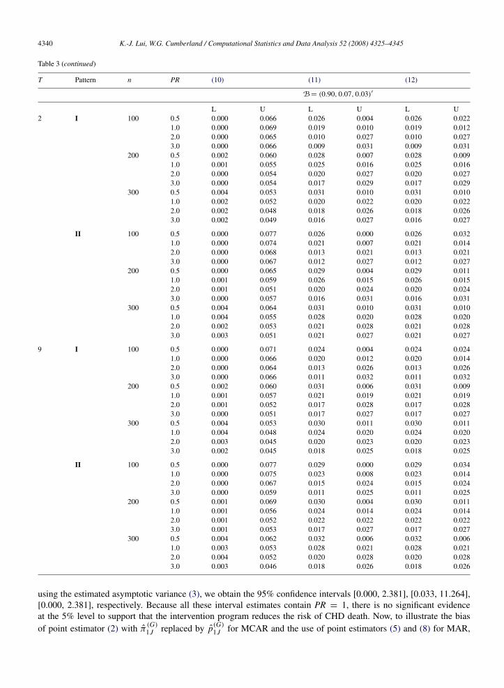
To study the bias of (10)–(12) we summarize in Table 3 the non-coverage probability in the lower and upper tailsof the resulting 95% confidence interval for the same set of configurations as those in Table 2. We note that usinginterval estimator (10) consistently produces a 95% confidence interval shifted to the left. We also note that usinginterval estimator (11) tends to produce a 95% confidence interval which shifts to the right for PR = 0.5, 1, but shiftsto the left for PR = 2, 3. We find that using interval estimator (12) improves the bias over using interval estimator (11)for PR = 0.5, 1, but has the bias nearly identical to the latter for PR = 2, 3. We also find that both interval estimators(11) and (12) consistently have less bias than interval estimator (10).

3.3. A numerical example

To illustrate the use of PR(2) and interval estimators (10)–(12) for data with no missingness, we first consider thedata in Table 4A taken from the multiple risk factor intervention trial (Multiple Risk Factor Intervention, 1982) forreducing the mortality of CHD. Eligible men aged 35–57 years at increased risk of death from CHD were randomlyassigned to either the intervention program or control group. Participants assigned to the intervention group wereprovided with dietary advice to reduce blood cholesterol, smoking cessation counseling, and hypertension medication,while participants assigned to the control group were referred to their usual physicians for treatment. However, onlythe treatment for cigarette smoking was actually effective as compared with those targeting blood cholesterol andhypertension. Because of the paucity of achieved difference in the other risk factors, we restrict our attention, as

K.-J. Lui, W.G. Cumberland / Computational Statistics and Data Analysis 52 (2008) 4325–4345 4337

Table 2The estimated coverage probability, the estimated average length of 95% confidence interval (in parenthesis), and the estimated proportion ofcases for which PR(6) does not exist (in brackets), for interval estimators (10)–(12) in the situations in which the distribution of subpopulations(P(Fi = C), P(Fi = A), P(Fi = N ))′ = A,B, where A = (0.70, 0.20, 0.10)′, B = (0.90, 0.07, 0.03)′; the parameter of dispersion T = 2, 9;the patterns of probabilities for non-missing outcomes I and II; the number of patients per treatment n = 100, 200, 300; and the underlyingproportion ratio of positive responses among compliers between the two treatments PR = 0.5, 1.0, 2.0, 3.0

T Pattern n PR (10) (11) (12) PR non-existence

A = (0.70, 0.20, 0.10)′

2 I 100 0.5 0.959(24.33) 0.978(5E193) 0.951(24.89) [0.041]1.0 0.941(87.94) 0.988(7E125) 0.969(15.33) [0.005]2.0 0.930(6.813)* 0.979(62E17) 0.978(7.900) [0.001]3.0 0.924(7.732)* 0.968(18E13) 0.968(9.151) [0.002]

200 0.5 0.952(0.982) 0.970(66E45) 0.948(1.204) [0.005]1.0 0.947(1.615) 0.978(61.96) 0.975(1.819) [0.000]2.0 0.941(2.703) 0.967(7.058) 0.967(2.930) [0.000]3.0 0.931(3.695)* 0.958(3.994) 0.958(3.968) [0.000]

300 0.5 0.951(0.789) 0.969(14E77) 0.957(0.896) [0.001]1.0 0.950(1.254) 0.967(1.340) 0.967(1.340) [0.000]2.0 0.946(2.070) 0.960(2.164) 0.960(2.164) [0.000]3.0 0.945(2.866) 0.960(2.980) 0.960(2.980) [0.000]

II 100 0.5 0.955(3.673) 0.973(8E297) 0.937(4.341)* [0.053]1.0 0.930(16.56)* 0.987(1E144) 0.953(17.49) [0.010]2.0 0.926(15.79)* 0.982(16E47) 0.979(16.89) [0.001]3.0 0.928(9.499)* 0.972(35E19) 0.972(10.89) [0.001]

200 0.5 0.942(1.050) 0.965(1E126) 0.929(1.324)* [0.010]1.0 0.939(1.696)* 0.976(32421) 0.970(1.936) [0.000]2.0 0.941(2.773) 0.968(3.015) 0.968(3.015) [0.000]3.0 0.939(3.803)* 0.961(4.222) 0.961(4.082) [0.000]

300 0.5 0.945(0.856) 0.964(93E22) 0.945(0.994) [0.002]1.0 0.948(1.344) 0.968(1.452) 0.968(1.450) [0.000]2.0 0.946(2.136) 0.963(2.238) 0.963(2.238) [0.000]3.0 0.945(2.903) 0.958(3.016) 0.958(3.016) [0.000]

9 I 100 0.5 0.962(1.693) 0.978(5E261) 0.953(2.260) [0.039]1.0 0.937(8.535)* 0.986(1E171) 0.965(9.348) [0.005]2.0 0.932(70.38)* 0.980(6E147) 0.978(71.46) [0.002]3.0 0.927(9.157)* 0.969(88E21) 0.969(10.51) [0.002]

200 0.5 0.955(0.993) 0.970(27E47) 0.950(1.217) [0.005]1.0 0.948(1.607) 0.977(35E75) 0.974(1.813) [0.000]2.0 0.939(2.667)* 0.966(2.888) 0.966(2.883) [0.000]3.0 0.941(3.700) 0.965(3.966) 0.965(3.960) [0.000]

300 0.5 0.956(0.793) 0.966(72E30) 0.956(0.903) [0.002]1.0 0.947(1.252) 0.971(1.338) 0.970(1.338) [0.000]2.0 0.947(2.074) 0.963(2.168) 0.963(2.168) [0.000]3.0 0.945(2.843) 0.960(2.953) 0.960(2.953) [0.000]

II 100 0.5 0.951(26.53) 0.978(2E260) 0.940(27.17) [0.055]1.0 0.931(13.32)* 0.986(8E218) 0.952(14.23) [0.010]2.0 0.929(85.40)* 0.985(3E217) 0.982(86.56) [0.001]3.0 0.925(11.18)* 0.969(52E44) 0.969(12.60) [0.001]

200 0.5 0.945(1.041) 0.971(2E285) 0.936(1.310)* [0.010]1.0 0.946(1.690) 0.977(444E9) 0.972(1.927) [0.001]2.0 0.936(2.759)* 0.967(2.989) 0.967(2.989) [0.000]3.0 0.940(3.783) 0.964(4.097) 0.964(4.071) [0.000]

300 0.5 0.944(0.853) 0.967(37E34) 0.950(0.993) [0.002]1.0 0.943(1.327) 0.969(21E28) 0.969(1.430) [0.000]2.0 0.948(2.150) 0.959(2.253) 0.959(2.253) [0.000]3.0 0.944(2.909) 0.960(3.024) 0.960(3.024) [0.000]

(continued on next page)

4338 K.-J. Lui, W.G. Cumberland / Computational Statistics and Data Analysis 52 (2008) 4325–4345

Table 2 (continued)

T Pattern n PR (10) (11) (12) PR non-existence

B = (0.90, 0.07, 0.03)′

2 I 100 0.5 0.934(1.068)* 0.970(2E36) 0.953(1.330) [0.114]1.0 0.931(1.792)* 0.970(2.232) 0.968(2.055) [0.105]2.0 0.935(3.061)* 0.963(3.420) 0.963(3.385) [0.112]3.0 0.934(4.325)* 0.960(4.907) 0.960(4.741) [0.114]

200 0.5 0.938(0.725)* 0.965(587E5) 0.963(0.796) [0.010]1.0 0.944(1.167) 0.959(1.232) 0.959(1.232) [0.011]2.0 0.945(1.967) 0.953(2.044) 0.953(2.044) [0.011]3.0 0.946(2.740) 0.955(2.833) 0.955(2.833) [0.009]

300 0.5 0.942(0.585) 0.959(0.620) 0.959(0.620) [0.001]1.0 0.946(0.922) 0.957(0.955) 0.957(0.955) [0.001]2.0 0.950(1.554) 0.955(1.592) 0.955(1.592) [0.001]3.0 0.950(2.151) 0.957(2.197) 0.957(2.197) [0.001]

II 100 0.5 0.923(1.149)* 0.973(2E270) 0.941(1.508) [0.077]1.0 0.926(1.922)* 0.972(153.5) 0.966(2.262) [0.071]2.0 0.932(3.180)* 0.966(3.547) 0.966(3.531) [0.063]3.0 0.933(4.452)* 0.961(14.53) 0.961(4.901) [0.065]

200 0.5 0.935(0.812)* 0.968(886E6) 0.961(0.916) [0.005]1.0 0.939(1.266)* 0.959(1.350) 0.959(1.350) [0.004]2.0 0.948(2.066) 0.956(2.155) 0.956(2.155) [0.004]3.0 0.943(2.809) 0.953(2.909) 0.953(2.909) [0.004]

300 0.5 0.932(0.653)* 0.959(0.716) 0.959(0.703) [0.000]1.0 0.942(1.010) 0.952(1.052) 0.952(1.052) [0.000]2.0 0.945(1.638) 0.952(1.683) 0.952(1.683) [0.000]3.0 0.946(2.240) 0.952(2.290) 0.952(2.290) [0.000]

9 I 100 0.5 0.929(1.061)* 0.972(11E47) 0.951(1.318) [0.115]1.0 0.934(1.791)* 0.968(4.827) 0.966(2.053) [0.109]2.0 0.936(3.096)* 0.961(3.655) 0.961(3.432) [0.109]3.0 0.934(4.331)* 0.957(5.221) 0.957(4.744) [0.108]

200 0.5 0.939(0.727)* 0.962(23E12) 0.960(0.800) [0.010]1.0 0.943(1.157) 0.960(1.221) 0.960(1.221) [0.011]2.0 0.947(1.955) 0.955(2.031) 0.955(2.031) [0.010]3.0 0.949(2.727) 0.955(2.819) 0.955(2.819) [0.011]

300 0.5 0.942(0.585) 0.959(0.620) 0.959(0.620) [0.001]1.0 0.949(0.927) 0.956(0.960) 0.956(0.960) [0.001]2.0 0.953(1.559) 0.957(1.597) 0.957(1.597) [0.001]3.0 0.953(2.164) 0.957(2.210) 0.957(2.210) [0.001]

II 100 0.5 0.923(1.156)* 0.971(1E24) 0.938(1.520)* [0.073]1.0 0.925(1.962)* 0.969(427.3) 0.963(2.304) [0.069]2.0 0.933(3.181)* 0.962(3.541) 0.962(3.533) [0.070]3.0 0.941(4.436) 0.964(4.999) 0.964(4.881) [0.065]

200 0.5 0.930(0.809)* 0.966(44.95) 0.959(0.913) [0.005]1.0 0.943(1.265) 0.962(1.349) 0.962(1.349) [0.004]2.0 0.948(2.059) 0.956(2.147) 0.956(2.147) [0.005]3.0 0.946(2.808) 0.956(2.908) 0.956(2.908) [0.003]

300 0.5 0.934(0.655)* 0.963(0.706) 0.962(0.705) [0.000]1.0 0.943(1.009) 0.952(1.052) 0.952(1.052) [0.000]2.0 0.944(1.634) 0.952(1.679) 0.952(1.679) [0.000]3.0 0.951(2.228) 0.956(2.279) 0.956(2.279) [0.000]

The symbol “*” indicates that the estimated coverage probability is less than the desired 95% confidence level by more than 1%.

done elsewhere (Mark and Robins, 1993; Sato, 2000; Matsui, 2005), to the effect of quitting cigarette smoking. Forillustrative purposes, we consider only patients smoking 30 or more cigarettes per day at the baseline (Table 4A).Based on the data in Table 4A, we obtain PR(2) to be 0.607, which suggests that participants in the interventionprogram have a risk of CHD death lower than those in the control group. When applying interval estimators (10)–(12)

K.-J. Lui, W.G. Cumberland / Computational Statistics and Data Analysis 52 (2008) 4325–4345 4339

Table 3The estimated non-coverage probability in the lower (L) and upper (U) tails of 95% confidence interval using interval estimators (10)–(12) inthe situations in which the distribution of subpopulation (P(Fi = C), P(Fi = A), P(Fi = N ))′ = A,B, where A = (0.70, 0.20, 0.10)′,B = (0.90, 0.07, 0.03)′; the parameter of dispersion T = 2, 9; the patterns of probabilities for non-missing outcomes I and II; the number ofpatients per treatment n = 100, 200, 300; and the underlying proportion ratio of positive responses among compliers between the two treatmentsPR = 0.5, 1.0, 2.0, 3.0

T Pattern n PR (10) (11) (12)

A = (0.70, 0.20, 0.10)′

L U L U L U2 I 100 0.5 0.000 0.041 0.021 0.001 0.021 0.027

1.0 0.000 0.059 0.011 0.001 0.011 0.0202.0 0.000 0.070 0.004 0.017 0.004 0.0183.0 0.000 0.076 0.002 0.030 0.002 0.030

200 0.5 0.000 0.048 0.029 0.001 0.029 0.0231.0 0.000 0.053 0.016 0.006 0.016 0.0092.0 0.000 0.059 0.011 0.022 0.011 0.0223.0 0.000 0.069 0.007 0.035 0.007 0.035

300 0.5 0.001 0.047 0.031 0.000 0.031 0.0131.0 0.000 0.049 0.023 0.010 0.023 0.0102.0 0.001 0.054 0.015 0.025 0.015 0.0253.0 0.000 0.055 0.011 0.029 0.011 0.029

II 100 0.5 0.000 0.045 0.027 0.000 0.027 0.0361.0 0.000 0.070 0.012 0.001 0.012 0.0352.0 0.000 0.074 0.005 0.013 0.005 0.0153.0 0.000 0.072 0.004 0.024 0.004 0.024

200 0.5 0.000 0.057 0.035 0.000 0.035 0.0361.0 0.000 0.061 0.021 0.003 0.021 0.0092.0 0.000 0.059 0.013 0.019 0.013 0.0193.0 0.000 0.061 0.011 0.028 0.011 0.028

300 0.5 0.001 0.054 0.036 0.000 0.036 0.0191.0 0.000 0.052 0.025 0.007 0.025 0.0072.0 0.001 0.054 0.015 0.022 0.015 0.0223.0 0.000 0.054 0.014 0.028 0.014 0.028

9 I 100 0.5 0.000 0.038 0.021 0.001 0.021 0.0261.0 0.000 0.063 0.013 0.002 0.013 0.0222.0 0.000 0.068 0.005 0.016 0.005 0.0173.0 0.000 0.073 0.003 0.028 0.003 0.028

200 0.5 0.000 0.044 0.029 0.001 0.029 0.0211.0 0.000 0.052 0.018 0.005 0.018 0.0082.0 0.000 0.061 0.011 0.024 0.011 0.0243.0 0.000 0.059 0.007 0.029 0.007 0.029

300 0.5 0.002 0.043 0.033 0.001 0.033 0.0111.0 0.000 0.053 0.019 0.010 0.019 0.0102.0 0.000 0.052 0.015 0.022 0.015 0.0223.0 0.000 0.055 0.010 0.030 0.010 0.030

II 100 0.5 0.000 0.049 0.022 0.000 0.021 0.0391.0 0.000 0.069 0.013 0.001 0.013 0.0362.0 0.000 0.071 0.005 0.010 0.005 0.0143.0 0.000 0.075 0.003 0.028 0.003 0.028

200 0.5 0.000 0.055 0.029 0.000 0.029 0.0351.0 0.000 0.054 0.021 0.002 0.021 0.0072.0 0.000 0.064 0.014 0.019 0.014 0.0193.0 0.000 0.060 0.011 0.026 0.011 0.026

300 0.5 0.002 0.054 0.033 0.000 0.033 0.0171.0 0.001 0.056 0.023 0.008 0.023 0.0082.0 0.001 0.052 0.019 0.022 0.019 0.0223.0 0.000 0.056 0.013 0.027 0.013 0.027

(continued on next page)

4340 K.-J. Lui, W.G. Cumberland / Computational Statistics and Data Analysis 52 (2008) 4325–4345

Table 3 (continued)

T Pattern n PR (10) (11) (12)

B = (0.90, 0.07, 0.03)′

L U L U L U2 I 100 0.5 0.000 0.066 0.026 0.004 0.026 0.022

1.0 0.000 0.069 0.019 0.010 0.019 0.0122.0 0.000 0.065 0.010 0.027 0.010 0.0273.0 0.000 0.066 0.009 0.031 0.009 0.031

200 0.5 0.002 0.060 0.028 0.007 0.028 0.0091.0 0.001 0.055 0.025 0.016 0.025 0.0162.0 0.000 0.054 0.020 0.027 0.020 0.0273.0 0.000 0.054 0.017 0.029 0.017 0.029

300 0.5 0.004 0.053 0.031 0.010 0.031 0.0101.0 0.002 0.052 0.020 0.022 0.020 0.0222.0 0.002 0.048 0.018 0.026 0.018 0.0263.0 0.002 0.049 0.016 0.027 0.016 0.027

II 100 0.5 0.000 0.077 0.026 0.000 0.026 0.0321.0 0.000 0.074 0.021 0.007 0.021 0.0142.0 0.000 0.068 0.013 0.021 0.013 0.0213.0 0.000 0.067 0.012 0.027 0.012 0.027

200 0.5 0.000 0.065 0.029 0.004 0.029 0.0111.0 0.001 0.059 0.026 0.015 0.026 0.0152.0 0.001 0.051 0.020 0.024 0.020 0.0243.0 0.000 0.057 0.016 0.031 0.016 0.031

300 0.5 0.004 0.064 0.031 0.010 0.031 0.0101.0 0.004 0.055 0.028 0.020 0.028 0.0202.0 0.002 0.053 0.021 0.028 0.021 0.0283.0 0.003 0.051 0.021 0.027 0.021 0.027

9 I 100 0.5 0.000 0.071 0.024 0.004 0.024 0.0241.0 0.000 0.066 0.020 0.012 0.020 0.0142.0 0.000 0.064 0.013 0.026 0.013 0.0263.0 0.000 0.066 0.011 0.032 0.011 0.032

200 0.5 0.002 0.060 0.031 0.006 0.031 0.0091.0 0.001 0.057 0.021 0.019 0.021 0.0192.0 0.001 0.052 0.017 0.028 0.017 0.0283.0 0.000 0.051 0.017 0.027 0.017 0.027

300 0.5 0.004 0.053 0.030 0.011 0.030 0.0111.0 0.004 0.048 0.024 0.020 0.024 0.0202.0 0.003 0.045 0.020 0.023 0.020 0.0233.0 0.002 0.045 0.018 0.025 0.018 0.025

II 100 0.5 0.000 0.077 0.029 0.000 0.029 0.0341.0 0.000 0.075 0.023 0.008 0.023 0.0142.0 0.000 0.067 0.015 0.024 0.015 0.0243.0 0.000 0.059 0.011 0.025 0.011 0.025

200 0.5 0.001 0.069 0.030 0.004 0.030 0.0111.0 0.001 0.056 0.024 0.014 0.024 0.0142.0 0.001 0.052 0.022 0.022 0.022 0.0223.0 0.001 0.053 0.017 0.027 0.017 0.027

300 0.5 0.004 0.062 0.032 0.006 0.032 0.0061.0 0.003 0.053 0.028 0.021 0.028 0.0212.0 0.004 0.052 0.020 0.028 0.020 0.0283.0 0.003 0.046 0.018 0.026 0.018 0.026

using the estimated asymptotic variance (3), we obtain the 95% confidence intervals [0.000, 2.381], [0.033, 11.264],[0.000, 2.381], respectively. Because all these interval estimates contain PR = 1, there is no significant evidenceat the 5% level to support that the intervention program reduces the risk of CHD death. Now, to illustrate the biasof point estimator (2) with π

(G)1J replaced by p(G)

1J for MCAR and the use of point estimators (5) and (8) for MAR,

K.-J. Lui, W.G. Cumberland / Computational Statistics and Data Analysis 52 (2008) 4325–4345 4341

Table 4The death incidence of coronary heart disease (CHD) during 7 years of follow-up between the intervention and control groups for the number ofcigarettes ≥30 per day at baseline in a randomized intervention trial

Group: Intervention ControlSmoking: Quit Not Quit Non-Quit Quit

(A) The observed frequency taken from a multiple risk factor intervention trialCHD Yes 5 39 47 1

No 532 1997 2388 214Total 537 2036 2435 215

(B) The expected frequency generated from Table 4A for the vector of the probability of non-missing outcome

(η(1)1 , η

(1)0 , η

(0)0 , η

(0)1 )′ = (0.65, 0.90, 0.90, 0.95)′

CHD Yes 3 35 42 1No 346 1797 2149 203Unknown 188 204 244 11Total 537 2036 2435 215

we consider the numerical data in Table 4B, which were obtained as the expected frequency from Table 4A whenwe assumed the probabilities of non-missing outcomes (η

(1)1 , η

(1)0 , η

(0)0 , η

(0)1 )′ = II (=(0.65, 0.90, 0.90, 0.95)′). On

the basis of these data (Table 4B), we obtain the estimates for the PR to be 0.351, 0.643, and 0.559, respectively,when applying estimator (2) with π

(G)1J replaced by p(G)

1J , and point estimators (5) and (8). Comparing these with the

estimate PR(2) = 0.607 based on Table 4A with no missing data illustrates that the bias of using (2) (with π(G)1J

replaced by p(G)1J ) is larger than those of estimators (5) and (8) under the assumed MAR. It should be pointed out that

the difference between the estimate 0.607 for Table 4A and the estimate 0.559 using (8) for Table 4B is actually dueto the round-off error in generation of non-missing data (needed to be in integers) and the precision of computation.Because some observed frequencies of CHD death in Table 4A are quite small (e.g., n(1)

1C + n(1)1A = 5 & n(0)

1A = 1), asmall round-off error (to be an integer) can have a relatively non-negligible impact on these cell probability estimates.This may explain the 5% difference between the estimate 0.607 which assumes no missing outcomes and the estimate0.558 using estimator (8) for data with missing outcomes (Table 4B). When using (10)–(12) for data in Table 4B, weobtain asymptotic 95% confidence intervals as [0.000, 2.399], [0.021, 15.008], and [0.000, 2.399]. As is expected,these interval estimates are slightly wider than the corresponding ones obtained for data with no missing outcomes(Table 4A). Note that the length of (11) is approximately 5–6 times those for (10) and (12) for data in both Table 4A,B. This is consistent with the previous findings that using interval estimator (11) with the logarithmic transformationtends to cause a substantial loss of precision as compared with the other two interval estimators (10) and (12).

4. Discussion

Table 1 indicates that the point estimator PR(5), which is derived under the assumption that non-missing outcomesdepend only on assigned treatments, can perform well even when the probability of non-missing outcomes actuallydepends on both assigned and received treatments (patterns I and II). Table 1 also shows that both the estimatedRB and MSE for estimators PR(5) and PR(8) are comparable under these patterns. In fact, the difference in both theestimated RB and MSE between these two estimators is quite small under all patterns considered here (Table 1). Thus,when the number of patients per treatment is small or moderate and we cannot calculate PR(8), we may consider usingPR(5) to estimate the underlying PR. In practice, we may not have prior knowledge to determine whether non-missingoutcomes depend only on assigned treatments or depend on both assigned and received treatments. An easy approachis to assume a logistic regression treating non-missing outcomes as the dependent variable, and both assigned andreceived treatments as independent covariates. We can apply the likelihood ratio test or Wald’s test to decide whichmodel is more appropriate for the observed data. Because use of PR(8) requires less restrictive assumption than useof PR(5), and because the differences in the estimated RB and MSE for these two estimators are quite small in allpatterns considered here, we may wish to use the former, especially when the number of patients per treatment is largeand there is an evidence that non-missing outcomes strongly depend on both assigned and received treatments.

4342 K.-J. Lui, W.G. Cumberland / Computational Statistics and Data Analysis 52 (2008) 4325–4345

When n = 100 and the subpopulation distribution is given by B′= (0.90, 0.07, 0.03), as noted previously, the

expected total of never-takers is only 3 (=100 × 0.03) patients per assigned treatment. Among these, even in thecase of no missing outcomes, we expect only 0.375 (=3 ×0.25 × 0.5) never-takers with a positive response in theexperimental treatment in our simulation. Following similar arguments, we can also show that the expected number ofalways-takers with a positive response per assigned treatment is small (<5) in our simulations as well. Nonetheless,our simulations suggest that interval estimators (10)–(12), although they are all derived from large sample theory, canperform reasonably well with respect to the coverage probability in these extreme cases. To further investigate theperformance of interval estimators (10)–(12) for even a sample size smaller than 100, we consider n = 50 and repeatsimulations for the same set of configurations as those considered in Table 2. We find that the interval estimator (10)becomes more liberal, while the interval estimator (11) becomes more conservative. We also find that the intervalestimator (12) still performs well; the coverage probabilities are all larger than or approximately equal to the desired95% confidence level. The probability of failing to use interval estimators (10)–(12) due to the non-existence of PR(8)can be, however, as large as approximately 40% when n = 50, PR = 0.5 and B′

= (0.90, 0.07, 0.03). Thus, we caninfer that as long as the MLE PR(8) exists, it may be still adequate for use of the interval estimator (12) for n = 50under the situations considered here.

When there are patients with missing outcomes, for simplicity we often assume MCAR, and use point estimator (2)with π

(G)1J replaced by p(G)

1J . This paper notes that use of this estimator can cause a large bias in point estimation undermodels with MAR. To alleviate this concern, this paper shows that one may use PR(5) or PR(8) when missingnessdepends on assigned treatments or both assigned and received treatments. On the other hand, we may encounterthe situation in which missingness may also depend on other factors such as gender or age. To account for theadditional effects of gender or age on missingness, we can apply stratified analysis with strata determined by acombination of gender and age categories. This leads us to consider the Mantel–Haenszel (MH) type estimator,PRM H =

∑l wl( p(1)

1C A|l/η(1)1|l − p(0)

1A|l/η(0)1|l )/

∑l wl( p(0)

1C N |l/η(0)0|l − p(1)

1N |l/η(1)0|l ), where wl = n1ln0l/(n1l + n0l), nGl

is the sample size for assigned treatment G in stratum l, p(G)1J |l and η

(G)R|l are simply calculated as p(G)

1J and η(G)R in (8)

by using the data from stratum l. When there are no patients with missing outcomes and when every patient complieswith his/her assigned treatment, the above PRM H reduces to the commonly-used MH estimator for the PR (Lui, 2004,2006b). Although we can also apply the delta method to derive the asymptotic variance of PRM H , the evaluation ofthe point estimator PRM H and the corresponding interval estimators for a non-compliance stratified RCT with missingoutcomes are beyond the scope of this paper and can be a future research topic.

Table 2 shows that when the number n of patients per treatment is not large, the interval estimator (10) basedon Wald’s statistic can lose accuracy, while the interval estimator (11) with the logarithmic transformation can loseprecision. The bias (Table 3) and short width of interval estimator (10) (Table 2) may account for the reason whyits coverage probability is lower than the nominal 95% confidence level. On the other hand, the wide length ofinterval estimator (11) may explain why its coverage probability tends to be larger than the 95%. To learn whetherour simulated results would be affected if we chose larger values for constants CC and CA (which must be, as notedbefore, bounded above by 1/PR), we concentrate our attention on the study of performance of interval estimators(10)–(12) around the PR of 1 (i.e., PR = 0.50, 1.0 and 2.0). We have repeated the entire Monte Carlo simulations bychoosing (CC , CA, CC ) = (0.40, 0.30, 0.35) and (0.40, 0.45, 0.50). Again, we have found that all the findings on therelative performance of these interval estimators still hold. When n 6 200 and PR = 0.50 (Table 2), Table 2 showsthat the estimated coverage probability of the interval estimator (12) can be less than the desired 95% confidence levelby around 2%. On the other hand, when n > 200 or PR > 1, the interval estimator (12) can consistently perform wellwith respect to the coverage probability in all the situations considered here, and hence we recommend its general useespecially for PR > 1. When the number of patients n per treatment is large (n = 300) and PR > 1, all these threeinterval estimators can perform well in most cases and the interval estimator (10) can be preferable to the others.

In summary, we have considered estimation of the PR under the RCT with non-compliance and missing outcomes.We have derived the MLE for the PR under models with MAR and evaluated the performance of these estimatorsin a variety of situations. We have noted that the estimator derived for MCAR can be subject to serious bias, whilethe estimators derived here can be of use for large sample sizes. We have further developed three asymptotic intervalestimators for the PR under MAR in which missingness depends on assigned and received treatments. We have notedthat the interval estimator based on Wald’s statistic tends to be liberal and biased, and the interval estimator withthe logarithmic transformation tends to be conservative. We have also demonstrated that the interval estimator (12)

K.-J. Lui, W.G. Cumberland / Computational Statistics and Data Analysis 52 (2008) 4325–4345 4343

generally performs well and has less bias than interval estimators (10) and (11) in many situations. Thus, werecommend interval estimator (12) for general use with a caution in the case of a small or moderate n and PR < 1.The results, findings, and discussions should have use for clinicians and biostatisticians when they encounter a non-compliance RCT with missing outcomes.

Acknowledgements

The authors wish to thank the two reviewers for many valuable comments and suggestions to improve the contentsand the clarity of this paper.

Appendix

A.1. Outlines for deriving the asymptotic variance Var(PR)(3) for no missing outcomes

Define f1(x1, x2) =x1x2

. When substituting π(1)1C = π

(1)1CA − π

(0)1A and π

(0)1C = π

(0)1CN − π

(1)1N for x1 and x2,we obtain

f1(x1, x2) = PR(2). Note that ∂ f1(x1, x2)/∂x1 = 1/x2 and ∂ f1(x1, x2)/∂x2 = −x1/x22 . When employing the delta

method (Agresti, 1990, pp. 420–424) to f1(x1, x2), we can show that

Var(PR) = {Var(π (1)1CA − π

(0)1A ) + PR2Var(π (0)

1CN − π(1)1N )

−2PRCov(π(1)1CA − π

(0)1A , π

(0)1CN − π

(1)1N )}/(π

(0)1CN − π

(1)1N )2, (A.1)

where

Var(π (1)1CA − π

(0)1A ) = π

(1)1CA(1 − π

(1)1CA)/n1 + π

(0)1A (1 − π

(0)1A )/n0,

Var(π (0)1CN − π

(1)1N ) = π

(0)1CN(1 − π

(0)1CN)/n0 + π

(1)1N (1 − π

(1)1N )/n1,

and

Cov(π(1)1CA − π

(0)1A , π

(0)1CN − π

(1)1N ) = π

(1)1CAπ

(1)1N /n1 + π

(0)1A π

(0)1CN/n0.

After substituting PR for PR and πi J ’s for πi J ’s, we obtain the estimated asymptotic variance Var(PR)(3).

A.2. Outlines for deriving the asymptotic variance Var(PR)(6) for MAR with missing outcomes depending on onlyassigned treatments

Note that PR(4) can be rewritten as

PR = H1/H2, (A.2)

where H1 = γ (0) p(1)1CA − γ (1) p(0)

1A and H2 = γ (1) p(0)1CN − γ (0) p(1)

1N .

Thus, we consider PR = H1/H2, where H1 = γ (0) p(1)1CA −γ (1) p(0)

1A and H2 = γ (1) p(0)1CN −γ (0) p(1)

1N . One can easilyshow that

∂PR/∂p(1)1CA = γ (0)/H2 (A.3)

∂PR/∂γ (1)= γ (0)

[p(0)1A p(1)

1N − p(1)1CA p(0)

1CN]/(H2)2 (A.4)

∂PR/∂p(1)1N = γ (0) H1/(H2)

2 (A.5)

∂PR/∂p(0)1CN = −γ (1) H1/(H2)

2 (A.6)

∂PR/∂γ (0)= −γ (1)

[p(0)1A p(1)

1N − p(1)1CA p(0)

1CN]/(H2)2 (A.7)

∂PR/∂p(0)1A = −γ (1)/H2. (A.8)

4344 K.-J. Lui, W.G. Cumberland / Computational Statistics and Data Analysis 52 (2008) 4325–4345

Furthermore, after a few algebraic manipulations, we obtain

ˆCov( p(1)1CA, γ (1)) = p(1)

1CA(1 − γ (1))/n1, (A.9)

ˆCov( p(1)1CA, p(1)

1N ) = − p(1)1CA p(1)

1N /n1, (A.10)

ˆCov( p(1)1N , γ (1)) = p(1)

1N (1 − γ (1))/n1, (A.11)

ˆCov( p(0)1CN, γ (0)) = p(0)

1CN(1 − γ (0))/n0, (A.12)

ˆCov( p(0)1CN, p(0)

1A) = − p(0)1CN p(0)

1A/n0, (A.13)

and

ˆCov( p(0)1A , γ (0)) = p(0)

1A(1 − γ (0))/n0. (A.14)

When employing the delta method again based on (A.3)–(A.14), we can obtain the estimated asymptotic varianceVar(PR)(6).

A.3. Outlines for deriving the asymptotic variance Var(PR)(9) for MAR with missing outcomes depending on assignedand received treatments

When substituting π(1)1C = p(1)

1CA/η(1)1 − p(0)

1A/η(0)1 and π

(0)1C = p(0)

1CN/η(0)0 − p(1)

1N /η(1)0 for x1 and x2 in f1(x1, x2), we

obtain f1(x1, x2) = PR(8). Following similar arguments as for deriving Var(PR)(A.1), we obtain

Var(PR) = {Var( p(1)1CA/η

(1)1 − p(0)

1A/η(0)1 ) + PR2Var( p(0)

1CN/η(0)0 − p(1)

1N /η(1)0 )

− 2PRCov( p(1)1CA/η

(1)1 − p(0)

1A/η(0)1 , p(0)

1CN/η(0)0 − p(1)

1N /η(1)0 )}/

(p(0)1CN/η

(0)0 − p(1)

1N /η(1)0 )2. (A.15)

Define f2(x1, x2, x3) =x1x3x2

. When substituting p(1)1CA, p(1)

1CA + p(1)2CA, and p(1)

+CA for x1, x2 and x3 in f2(x1, x2, x3),

we obtain f2(x1, x2, x3) = p(1)1CA/η

(1)1 . Note that ∂ f2(x1, x2, x3)/∂x1 = x3/x2, ∂ f2(x1, x2, x3)/∂x2 = −x1x3/x2

2 , and∂ f2(x1, x2, x3)/∂x3 = x1/x2. Thus, by applying the delta method to the function f2(x1, x2, x3), we obtain after a fewalgebraic manipulations,

Var( p(1)1CA/η

(1)1 ) = [ p(1)

1CA(1 − p(1)1CA) + (π

(1)1CA)2η

(1)1 (1/ p(1)

+CA − η(1)1 )

− 2π(1)1CA( p(1)

1CA)(1/ p(1)+CA − η

(1)1 ) + 3( p(1)

1CA)2(1 − p(1)+CA)/ p(1)

+CA

− 2π(1)1CA( p(1)

1CA)η(1)1 (1 − p(1)

+CA)/ p(1)+C A]/[n1(η

(1)1 )2

]. (A.16)

Applying the same arguments as for deriving for (A.16), we can derive the estimated asymptotic variancesVar( p(1)

1N /η(1)0 ), Var( p(0)

1CN/η(0)0 ), and Var( p(0)

1A/η(0)1 ).

Define h1(x) =x1x3x2

and h2(x) =x4x6x5

, where x = (x1, x2, x3, . . . , x6)′. When substituting p(1)

1CA, p(1)1CA + p(1)

2CA,

and p(1)+CA for x1, x2 and x3 in h1(x), as well as substituting p(1)

1N , p(1)1N + p(1)

2N , and p(1)+N for x4, x5 and x6 in h2(x),

we obtain h1(x) = p(1)1CA/η

(1)1 and h2(x) = p(1)

1N /η(1)0 . Using the delta method for the function of random vectors

(Agresti, 1990, p. 424) to (h1(x), h2(x))′, we can obtain the estimated asymptotic covariance after a few algebraicmanipulations:

ˆCov( p(1)1CA/η

(1)1 , p(1)

1N /η(1)0 ) = −π

(1)1CAπ

(1)1N /n1. (A.17)

Similarly, we can obtain the estimated asymptotic covariance

ˆCov( p(0)1CN/η

(0)0 , p(0)

1A/η(0)1 ) = −π

(0)1CN π

(0)1A /n0. (A.18)

On the basis of (A.15)–(A.18), we obtain the estimated asymptotic variance Var(PR)(9).

K.-J. Lui, W.G. Cumberland / Computational Statistics and Data Analysis 52 (2008) 4325–4345 4345

References

Agresti, A., 1990. Categorical Data Analysis. Wiley, New York.Anbar, D., 1983. The relative efficiency of Zelen’s prerandomization design for clinical trials. Biometrics 39, 711–718.Angrist, J.D., Imbens, G.W., Rubin, D.B., 1996. Identification of causal effects using instrumental variables. Journal of the American Statistical

Association 91, 444–456.Barnard, J., Frangakis, G.E., Hill, J.E., Rubin, D.B., 2003. Principal stratification approach to broken randomized experiments: A case study of

school choice voucher in New York City. Journal of the American Statistical Association 98, 299–311.Bernhard, G., Compagnone, D., 1989. Binary data in prerandomized designs. Biometrical Journal 31, 29–33.Brunner, E., Neumann, N., 1985. On the mathematical basis of Zelen’s prerandomized designs. Methods of Information in Medicine 24, 120–130.Casella, G., Berger, R.L., 1990. Statistical Inference. Duxbury, Belmont, CA.Fleiss, J.L., 1981. Statistical Methods for Rates and Proportions. Wiley, New York.Frangakis, C.E., Rubin, D.B., 1999. Addressing complications of intention-to-treat analysis in the combined presence of all-or-none treatment-

noncompliance and subsequent missing outcomes. Biometrika 86, 365–379.Katz, D., Baptista, J., Azen, S.P., Pike, M.C., 1978. Obtaining confidence intervals for the risk ratio in cohort studies. Biometrics 34, 469–474.Li, F., Frangakis, C.E., 2005. Designs in partially controlled studies: Messages from a review. Statistical Methods in Medical Research 14, 417–431.Lui, K.-J., 2002. Notes on estimation of the general odds ratio and the general risk difference for paired-sample data. Biometrical Journal 44,

957–968.Lui, K.-J., 2004. Statistical Estimation Epidemiological Risk. Wiley, New York.Lui, K.-J., 2006a. In: Chow, S.-C. (Ed.), Risk Ratio Analysis, 2nd edn., Revised and Expanded. In: Encyclopedia of Biopharmaceutical Statistics,

Marcel Dekker, New York.Lui, K.-J., 2006b. A Monte Carlo evaluation of five interval estimators for the relative risk in sparse data. Biometrical Journal 48, 131–143.Lui, K.-J., 2007. Interval estimation of risk ratio in the simple compliance randomized trial. Contemporary Clinical Trials 28, 120–129.Lui, K.-J., 2008. Estimation of proportion ratio in non-compliance randomized trials with repeated measurements in binary data. Statistical

Methodology 5, 129–141.Lui, K.-J., Lin, C.-D., 2003. Interval estimation of treatment effects in double consent randomized design. Statistica Sinica 13, 179–187.Mark, S.D., Robins, J.M., 1993. A method for the analysis of randomized trials with compliance information: An application to the multiple risk

factor intervention trial. Controlled Clinical Trials 14, 79–97.Matsui, S., 2005. Stratified analysis in randomized trials with noncompliance. Biometrics 61, 816–823.Matsuyama, Y., 2002. Correcting for non-compliance of repeated binary outcomes in randomized clinical trials: Randomized analysis approach.

Statistics in Medicine 21, 675–687.Matts, J., McHugh, R., 1987. Randomization and efficiency in Zelen’s single consent design. Biometrics 43, 885–894.Matts, J.P., McHugh, R.B., 1993. Precision estimation in Zelen’s single-consent design. Biometrical Journal 35, 65–72.McDonald, C.J., Hui, S.L., Tierney, W.M., 1992. Effects of computer reminders for influenza vaccination on morbidity during influenza epidemics.

M.D. Computing 9, 304–312.McHugh, R., 1984. Validity and treatment dilution in Zelen’s single consent design. Statistics in Medicine 3, 215–218.Multiple Risk Factor Intervention Trial Research Group, 1982. Multiple risk factor intervention trial: Risk factor changes and mortality results.

Journal of the American Medical Association 248, 1465–1477.SAS Institute Inc., 1990. SAS Language, Reference Version 6, 1st edn. SAS Institute, Cary, NC.Sato, T., 2000. Sample size calculations with compliance information. Statistics in Medicine 19, 2689–2697.Sato, T., 2001. A method for the analysis of repeated binary outcomes in randomized clinical trials with non-compliance. Statistics in Medicine 20,

2761–2774.Sheps, M.C., 1958. Shall we count the living or the dead? New England Journal of Medicine 259, 1210–1214.Sheps, M.C., 1959. An examination of some methods of comparing several rates or proportions. Biometrics 15, 87–97.Sommer, A., Zeger, S.L., 1991. On estimating efficacy from clinical trials. Statistics in Medicine 10, 45–52.Yau, L.H.Y., Little, R.J., 2001. Inference for complier-average causal effect from longitudinal data subject to noncompliance and missing data, with

application to a job training assessment for the unemployed. Journal of the American Statistical Association 96, 1232–1244.Zelen, M., 1979. A new design for randomized clinical trials. The New England Journal of Medicine 300, 1242–1245.Zelen, M., 1986. Response. Journal of Chronic Disease 39, 247–249.Zelen, M., 1990. Randomized consent designs for clinical trials: An update. Statistics in Medicine 9, 645–656.Zhou, X.-H., Li, S.M., 2006. ITT analysis of randomized encouragement design studies with missing data. Statistics in Medicine 25, 2737–2761.