Note on Transformations of Quadratic Equations in Algorithms in Mathematical Cuneiform Texts

of 34

A Note on Transformations of Quadratic Equations in Algorithms in

Mathematical Cuneiform Texts

by Robert L. Baber, 2008 December, revised 2009 January 3 – 22, May 19 [email protected], http://office.RLBaber.de

Goal of this investigation The goal of this examination of Babylonian and Mesopotamian algorithms for calculating the positive roots of quadratic equations was to identify (1) the conditions under which a transformed equation was first solved and (2) what transformations were applied to the original equations.

Summary Algorithms for solving quadratic equations were taken from the research literature on Mesopotamian mathematical cuneiform texts. The algorithms examined included (1) complete algorithms for solving quadratic equations only and (2) extracts of algorithms for solving larger problems of which quadratic equations were only parts.

To find a positive root of a quadratic equation

a•s2 + b•s + c = 0

every algorithm examined (with the possible exception of algorithm 6, tablet B.M. 13901, No. 23) calculated a positive root of the equation

s12 + b•s1 + a•c = 0

and then (if a≠1) multiplied the root s1 by 1/a to find the root s of the original equation. With the possible exception cited above, no other type of transformation was found among the algorithms examined.

The above transformation results in a quadratic equation in which the coefficient of the quadratic term is 1 and the coefficient b of the linear term is unchanged. The algorithm first finds the value of (a•s) that satisfies the first equation above and then effectively divides that value by the parameter a to obtain the desired solution s.

When a=1, the original equation is already in the transformed form. Two calculations (multiplying c by a and multiplying s1 by 1/a) reduce to multiplication by 1 and are, therefore, not performed.

[Berriman] mentions on page 186 that quadratic equations solved in Babylonian texts were transformed in this particular way, but it is not clear whether that comment applies only to algorithms in that paper or to Mesopotamian algorithms more generally. [Ritter] states on page 66 that the equation solved on the lower half of page 65 was transformed to an equation of the form s1

2+s1+…, i.e. not as specified above, but that statement is not correct. As shown in this note, that equation was also transformed as described above.

The reason for solving a transformed quadratic equation first is not completely clear. A slight modification of the standard procedure can calculate the root of the original equation directly. The modification would eliminate the multiplication by 1/a at the end of the algorithm at the expense of introducing it in an earlier step to calculate b/a. Multiplying c by a would be replaced by multiplying c by 1/a. Thus, the number of computational steps would remain the same. The transformational approach does, however, have one advantage over calculating the root of a quadratic equation directly: Only one division (multiplication by a reciprocal), not two, is required, reducing the guesswork needed when the sexagesimal representation of the

mailto:[email protected]?subject=Transformations%20of%20Quadratic%20Equations%20in%20Algorithms%20in%20Mathematical%20Cuneiform%20Texts�

http://office.rlbaber.de/�

of 34

reciprocal (e.g. 1/7) does not end. Whether or not this was the actual reason for transforming quadratic equations in Mesopotamian mathematics is a matter of speculation.

Overview of examined algorithms The table below contains one entry for each algorithm examined. Each entry contains a unique identification of the algorithm and the parameters of the original quadratic equation whose positive root the algorithm calculates. Some algorithms first find the positive root of a transformed equation and then transform the solution found to obtain the solution of the original equation. Where applicable, the parameters of such a transformed equation are also shown in the table below. These parameters are shown both as numbers and as functions of the parameters in the original equation.

Abbreviations used in the headers in the table below are defined as follows. The variable whose value is calculated by the algorithm in question is named s (see “Notation” below). In the transformed equations, the variable is named s1. Similarly, the parameters of the equations are named a, b, and d or a1, b1 and d1.

ID: identification of the particular Babylonian algorithm parameters in the original equation: a•s2 + b•s − d = 0, where a≠0 parameters in the transformed equation *: s1

2 + b1•s1 − d1 = 0

All numbers in the table below are in the decimal (base 10) system.

ID

original parameters (numerical)

transformation transformed parameters *

numerical as functiona b d numerical function a1 b1 d1 a1 b1 d1

1 1 1 3/4 none not applicable 2 1 ‒1 870 none not applicable 3 2/3 1/3 1/3 s=s1/(2/3) s=s1/a ** 1 1/3 2/9 1 b a•d4 1 ‒225 ‒8100 none not applicable 5 13/9 20/3 1500 s=s1/(13/9) s=s1/a ** 1 20/3 6500/3 1 b a•d6 1 4 25/36 none (see ID 6) not applicable 7 1800 ‒150 375 s=s1/1800 s=s1/a ** 1 ‒150 675000 1 b a•d8 1 ‒10 600 none not applicable 9 1 ‒1300 ‒360000 none not applicable 10 1 ‒26/12 ‒1 none not applicable 11 13/9 ‒40/3 900 s=s1/(13/9) s=s1/a ** 1 ‒40/3 1300 1 b a•d12 13/9 80/3 2100 s=s1/(13/9) s=s1/a ** 1 80/3 9100/3 1 b a•d13 13/9 140/3 2700 s=s1/(13/9) s=s1/a ** 1 140/3 3900 1 b a•d14 1 ‒29 ‒210 none not applicable 15 1 100 5600 none not applicable 16 5/8 15 1600 s=s1/(5/8) s=s1/a ** 1 15 1000 1 b a•d17 4 1/3 7/6 s=s1/4 s=s1/a ** 1 1/3 14/3 1 b a•d18 4 8/3 7/3 s=s1/4 s=s1/a ** 1 8/3 28/3 1 b a•d19 2/3 5/18 25/3 s=s1/(2/3) s=s1/a ** 1 5/18 50/9 1 b a•d20 1 ‒5/18 50/9 none not applicable 21 7 ‒17/6 ‒1/6 s=s1/7 s=s1/a ** 1 ‒17/6 ‒7/6 1 b a•d22 1 ‒17/6 ‒7/6 none not applicable 23 22464 ‒720 3600 s=s1/22464 s=s1/a ** 1 ‒720 80870400 1 b a•d24 68580 ‒1260 7200 s=s1/68580 s=s1/a ** 1 ‒1260 493776000 1 b a•d25 34020 ‒540 3600 s=s1/34020 s=s1/a ** 1 ‒540 122472000 1 b a•d

of 34

26 1800 ‒150 375 s=s1/1800 s=s1/a ** 1 ‒150 675000 1 b a•d27 1 5/6 25/3 none not applicable 28 1 ‒35/6 ‒25/3 none not applicable 29 1 ‒13/12 ‒7/24 none not applicable

* The transformed equations are normalized to a1=1. It is not possible to determine the transformed parameters a1, b1 and d1 precisely, only the ratios b1/a1 and d1/a1. This is due to the fact that

s12 + b1•s1 − d1 = 0

= k•s1

2 + k•b1•s1 − k•d1 = 0

for any non-zero number k. Consequently, all such equations have the same solutions for s1.

** This transformation is equivalent to solving the quadratic formula for the original equation for (a•s) and then dividing by a (multiplying by the reciprocal of a) to obtain the desired value for s.

Notation: Occasionally, the variable name x is used in the cited literature with a different meaning or connotation than the variable in a general quadratic equation. Therefore, the variable name s is used in this article to reduce possible misunderstanding or confusion.

The transformation With the possible exception of algorithm 6, the Mesopotamian algorithms examined in this note solve the initial quadratic equation

a•s2 + b•s + c = 0

by first solving the intermediate equation

s12 + b•s1 + a•c = 0

Effectively, the initial quadratic equation is transformed by the change of variable s=s1/a (and multiplying the entire equation by a). Finally, each algorithm transforms the solution s1 of the intermediate equation back to the solution s of the initial equation by multiplying s1 by the reciprocal of a. (Multiplying by the reciprocal was the normal way of dividing in Mesopotamian arithmetic.)

Note that this transformation converts the initial quadratic equation into an intermediate one in which the coefficient of the quadratic term is 1 and the coefficient of the linear term is unchanged – not necessarily 1.

A different but equivalent view of this transformation is helpful in understanding it. Multiplying the original equation above by a results in

a2•s2 + b•a•s + a•c = 0

which can be rewritten as

(a•s)2 + b•(a•s) + a•c = 0

The quadratic formula can be applied to this equation to find the solution for (a•s). Multiplying that solution by 1/a gives the solution s of the original equation.

The term (a•s) is s1.

Multiplying s by a is the important characteristic of the above transformation. If, in addition, a constant is added, an equivalent result is obtained. If the additive constant is b/2, even the same algorithm will arise. For example, if s2=a•s+b/2, (i.e. if s2=s1+b/2) then

of 34

a•s2 + b•s + c = 0

becomes

s22 − (b/2)2 + a•c = 0

or, equivalently,

s22 = (b/2)2 − a•c

and

s2 = ((b/2)2 − a•c)1/2

In the Mesopotamian algorithms for calculating the root of a quadratic equation, the step that extracts the square root calculates s2 and the following step, which adds or subtracts b/2, calculates s1. The final step divides s1 by a (by multiplying s1 by 1/a) to calculate s, the desired final result.

The transformation s2=a•s+b/2 is mentioned in [Friberg1] in § 5.7 c, on page 573, column 2, at the end of the first paragraph. In that passage, the variables and parameters are named differently.

Both of the above transformations for s1 and s2 are embedded in the contemporary quadratic formula, whose derivation is based on the concept of completing the square.

Analyzing an algorithm for calculating the root of a quadratic equation With the possible exception of algorithm 6, every Mesopotamian algorithm for calculating the root of a quadratic equation examined in this project exhibited the following structure. This structure directly reflects the quadratic formula we know.

Calculational step expression for value calculated

calculate a a calculate d d multiply a and d a•d calculate b b calculate b/2 b/2 square b/2 (b/2)2 add (subtract if negative) a•d to (b/2)2 (b/2)2 + a•d square root of previous result ((b/2)2+ a•d)1/2 add (or subtract ) b/2 to/from previous result –b/2 + ((b/2)2 + a•d)1/2 divide previous result by a (–b/2 + ((b/2)2 + a•d)1/2)/a

If the value of the parameter a is 1, the steps calculating a, multiplying a and d, and dividing by a will be missing.

Note that squaring a term (often described as multiplying a term by itself) occurs in this type of algorithm only once. Similarly, calculating the square root of a number also occurs only once. Other operations such as adding, subtracting, multiplying, taking the reciprocal of a number, etc. can occur several times in several steps.

When analyzing an algorithm believed to calculate the root of a quadratic equation, look first for the square root operation. Immediately following it will be a step adding or subtracting the term b/2. The result of this addition or subtraction will, if the original quadratic equation was not already in the transformed form (i.e., if a≠1), be divided by (multiplied by the reciprocal of) the parameter a, the coefficient of the quadratic term in the original equation. This will enable the analyst to identify both parameters a and b. Before the square root operation will be steps that square the b/2 term and add it to another term (the term a•d). These steps will

of 34

enable one to confirm the b/2 term and identify d. The step multiplying a and d can be used to confirm the values of a and d already identified.

If the structure outlined above is not found, the square root and squaring operations most likely are not involved in calculating the root of a quadratic equation. The absence of the squaring and square root operations is a clear indication that the algorithm does not calculate the root of a quadratic equation.

All algorithms examined in this project exhibit the above general pattern. As mentioned in the section “Calculating the root directly” below, the above algorithm can be modified to calculate the root of any quadratic equation directly, without the final division step. Such an algorithm would calculate b/(2•a) instead of b/2 and would calculate d/a instead of a•d. If the calculations differ from the above in this way, an algorithm not transforming the quadratic equation to be solved may have been identified. As yet, there is no reason to believe or speculate that such an algorithm will be found.

Calculating the root directly A Mesopotamian style algorithm for directly calculating the solution of a general quadratic equation can be derived by modifying slightly the initialization in the algorithm above. If the equation to be solved is

as2 + bs – d = 0

then the positive solution for s is

s = – (b/(2a)) + ((b/(2a))2 + (d/a))1/2

The standard Mesopotamian algorithm can be modified so that (d/a) is calculated instead of a•d and (b/(2•a)) is calculated in addition to (b/2) in the early part of the algorithm. Then the multiplication of s1 by 1/a can be eliminated.

of 34

Examination of the individual algorithms Translations: In the algorithms below, the descriptions of the individual steps are mathematically accurate translations of the material in the cited sources into contemporary mathematical terminology. No attempt has been made to capture the literary style of either the Akkadian originals or the intermediate translations, of which there may be several. Thus, the descriptions below of the steps in the algorithms do not reflect Babylonian views of the mathematics involved.

ID: 1, tablet B.M. 13901, No. 1 Quadratic equation to be solved: s2 + s – d = 0

Sources: [Ritter] This algorithm is on pages 62-63.

[Berriman] This algorithm is on page 185.

Parameter: The particular calculation shown in the source of this algorithm is for the value 0;45 (base 60), i.e. for 3/4 (base 10 fraction) for d.

result (60) result (10) result expressed Step for given d for given d as a function of d

1. set 1 1;0 1 1 2. subtract half of 1 from result of step 1 0;30 1/2 1/2 3. multiply result of step 2 by itself 0;15 1/4 1/4 4. add result of step 3 to d 1;0 1 1/4 + d 5. take square root of result of step 4 1;0 1 (1/4 + d)1/2 6. subtract result of step 2 from result of step 5 0;30 1/2 (1/4 + d)1/2 – 1/2

The result of step 6 is the quadratic formula for the positive root of the equation s2+s–d=0.

This algorithm does not transform the original quadratic equation internally into another equation.

of 34

ID: 2, tablet B.M. 13901, No. 2 Quadratic equation to be solved: s2 – s – d = 0

Sources: [Ritter] This algorithm is on the upper part of page 65.

[Berriman] This algorithm is on p. 186.

Parameter: The particular calculation shown in the source of this algorithm is for the value 14 30 (base 60), i.e. for 870 (base 10) for d.


1. set 1 1;0 1 1 2. subtract half of 1 from result of step 1 0;30 1/2 1/2 3. multiply result of step 2 by itself 0;15 1/4 1/4 4. add result of step 3 to d 14 30;15 870.25 1/4 + d 5. take square root of result of step 4 29;30 29.5 (1/4 + d)1/2 6. add result of step 2 to result of step 5 30; 30 (1/4 + d)1/2 + 1/2

The result of step 6 is the quadratic formula for the positive root of the equation s2–s–d=0.


of 34

ID: 3, tablet B.M. 13901, (No. 3?) Quadratic equation to be solved: (2/3)•s2 + (1/3)•s – d = 0

Source: [Ritter] This algorithm is on the lower part of page 65.

Parameter: The particular calculation shown in the source of this algorithm is for the value 0;20 (base 60), i.e. for 1/3 (base 10) for d.


1. set 1 1;0 1 1 2. subtract third of 1 from result of step 1 0;40 2/3 2/3 3. multiply result of step 2 by d 0;13 20 2/9 2d/3 4. take away half of 1/3 0;10 1/6 1/6 5. multiply result of step 4 by itself 0;1 40 1/36 1/36 6. add result of step 3 to result of step 5 0;15 1/4 1/36 + 2d/3 7. square root of result of step 6 0;30 1/2 (1/36 + 2d/3)1/2

8. subtract result of step 4 from result of step 7 0;20 1/3 (1/36 + 2d/3)1/2 – 1/6 9. reciprocal of result of step 2 1;30 3/2 3/2 10. multiply result of step 9 by result of step 8 0;30 1/2 ((1/36 + 2d/3)1/2 – 1/6)•(3/2)

The result of step 10 is equal to ((1/16 + 3d/2)1/2 – 1/4), which is the quadratic formula for the positive root of the original equation (2/3)•s2+(1/3)•s–d=0.

This algorithm transforms the original quadratic equation internally into the equation s1

2+(1/3)•s1–2d/3=0 (or any multiple thereof), whose solution is the result of step 8. The transformation is s=s1/a, in this particular case, s=(3/2)•s1.

of 34

ID: 4, tablet B.M. 85194, No. 25 Quadratic equation to be solved: s2 – 225•s + c = 0, more generally referred to below as s2+b•s+c=0

The subject of the algorithm cited here is a more encompassing problem, of which solving this quadratic equation is a part. The algorithm below shows only those steps in the original algorithm that are relevant to the quadratic equation above.

Source: [Berriman] This algorithm is on pages 188-189.

Parameter: The particular calculation shown in the source of this algorithm is for the value 8100 (base 10) for c.

result (10) result expressed Step for given c as a function of b, c

1. … … … 2. calculate b/2 112.5 b/2 3. calculate b 225 b 4. calculate c 8100 c 5. square b/2 12656.25 (b/2)2 6. subtract c from (b/2)2 4556.25 (b/2)2 – c 7. square root of result of step 6 67.5 ((b/2)2 – c)1/2 8. subtract result of step 7 from b/2 45 b/2 – ((b/2)2 – c)1/2 9. … … …

The result of step 8 is the quadratic formula for the smaller root of the original equation above.


of 34

ID: 5, tablet B.M. 13901, No. 14 Quadratic equation to be solved: (13/9)•s2 + (20/3)•s – d = 0, more generally referred to below as a•s2+b•s–d=0


Source: [Berriman] This algorithm is on page 187.

Parameter: The particular calculation shown in the source of this algorithm is for the value 1500 (base 10) for d.

result (10) result expressed Step for given d as a function of a, b, d

1. … … … 2. calculate d 1500 d 3. … … … 4. calculate a 13/9 a 5. calculate a•d 6500/3 a•d 6. calculate b/2 10/3 b/2 7. square b/2 100/9 (b/2)2 8. add results of steps 7 and 5 19600/9 (b/2)2 + a•d 9. square root of result of step 8 140/3 ((b/2)2 + a•d)1/2 10. subtract b/2 from result of step 9 130/3 ((b/2)2 + a•d)1/2 – b/2 11. multiply the result of step 10 by the reciprocal of a 30 (((b/2)2 + a•d)1/2 – b/2)/a

The result of step 11 is equal to ((b/(2•a))2 + d/a)1/2 – b/(2•a), which is the quadratic formula for the positive root of the original equation.


2+b•s1–a•d=0 (or any multiple thereof), whose solution is the result of step 10. The transformation is s=s1/a, in this particular case, s=(9/13)•s1.

of 34

ID: 6, tablet B.M. 13901, No. 23 Quadratic equation to be solved: s2 + 4•s – d = 0 [1]

or (1/2)•s2 + 2•s – d/2 = 0 [2]

or (s/2)2 + 2•(s/2) – d/4 = 0 [3]

or s12 + 2•s1 – d/4 = 0 [4]

see “Comments” below.


[Friberg2] This algorithm is on pages 311-312.

[Høyrup] This algorithm is on page 2.

[Neugebauer3] This algorithm is on page 9.

Parameter: The particular calculation shown in the source of this algorithm is for the value 0;41,40 (base 60), i.e. for 25/36 (base 10) for d.


1. set 4 4 4 4 2. reciprocal of 4 0;15 1/4 1/4 3. multiply result of step 2 and d 0;10,25 25/144 d/4 4. add 1 to result of step 3 1;10,25 169/144 1+d/4 5. square root of result of step 4 1;5 13/12 (1+d/4)1/2 6. subtract 1 from result of step 5 0;5 1/12 (1+d/4)1/2 – 1 7. multiply result of step 6 by 2 0;10 1/6 (4+d)1/2 – 2

Comments: When examining a Mesopotamian algorithm originally in cuneiform, an expression in modern mathematical form for the result of each step can always be deduced. Because the operands involved are referred to by value, it is sometimes unclear whether a numerical constant or the value of a parameter (or a previous result) of the problem is meant, but inserting the numerical value into the modern expression always leads to a correct expression. On the other hand, the original Mesopotamian author’s intention for what the algorithm should calculate can remain speculative, that is, the modern form for the original quadratic equation to be solved can remain unclear. In the case of every other algorithm examined in this project one of the several possibilities stands out as significantly more meaningful and likely than the others. In the case of this algorithm ID 6, the choice among the several possibilities is not really clear.

Equation [1] above corresponds most closely with the original statement of the problem: the sum of the area and the four sides of a square is 25/36. However, little in the algorithm itself is consistent with the choice of equation [1] as the equation whose solution the author of the algorithm actually wanted to calculate.

The fact that the first reference to the parameter d effectively divides it by 4 suggests that the original intention was not to solve equation [1] but rather to solve either equation [2], [3] or [4]. Especially the goal represented by equations [3] and [4] , i.e. to solve initially for half the length of the side, not the length of the side itself, is consistent with [Berriman] and the diagrams in [Friberg2] and [Høyrup]. Therefore, I categorize this algorithm as not based on a transformation of the original quadratic equation to be solved, admitting that this choice can be contested.

of 34

Note that equation [4] is the same as equation [3] with s1=s/2. The standard transformation identified in all the other algorithms examined in this project would transform equation [2] into equation [4]. Note also that equations [1], [2] and [3] are multiples of one another, i.e. are effectively the same equation. Still other multiples are conceivable, but there is little or no evidence to suggest considering them seriously.

From the expression for the result obtained in step 6 of the algorithm it is clear that this result is the solution of equation [4], i.e. is half of the length of the side of the square in question. The multiplication in step 7 adjusts this result to the full length of the side.

Note further that equation [1] is already in the transformed form. Its solution could have been calculated in the same way as other algorithms examined in this note, with no more steps in the calculation than in this algorithm.

[Neugebauer3] suggests on page 14 that the scribe might have misinterpreted the problem to be solved (“Ich halte es nicht für ausgeschlossen, daß die ganze Aufgabe vom Schreiber falsch interpretiert wurde …”). Also other aspects of this problem and its solution are identified as questionable in this passage in [Neugebauer3].

of 34

ID: 7, from a tablet in the Museum of Strasbourg University Quadratic equation to be solved: 1800•s2 – 150•s – d = 0, more generally referred to below as a•s2+b•s–d=0




result (10) result expressed Step for given d as a function of a, b, d

1. … 2. calculate a 1800 a 3. calculate a•d 675000 a•d 4. calculate ⎪b⎪ 150 ⎪b⎪ 5. multiply result of step 4 by 1/2 75 ⎪b/2⎪ 6. square result of step 5 5625 (b/2)2 7. add results of steps 6 and 3 680625 (b/2)2 + a•d 8. square root of result of step 7 825 ((b/2)2 + a•d)1/2 9. add result of step 5 to result of step 8 900 ((b/2)2 + a•d)1/2 +⎪b/2⎪ 10. reciprocal of a (result of step 2) 1/1800 1/a 11. multiply result of step 9 by result of step 10 1/2 (((b/2)2 + a•d)1/2 +⎪b/2⎪)/a … …

The result of step 11 is equal to ((b/(2•a))2 + d/a)1/2 +⎪b/(2•a)⎪, which is the quadratic formula for the positive root of the original equation above to be solved.

This algorithm transforms the original quadratic equation internally into the equation s12–

150•s1–a•d=0 (or any multiple thereof), whose solution is the result of step 9. The transformation is s=s1/a, in this particular case, s=s1/1800.

of 34

ID: 8, tablet B.M. 13901, No. 9 Quadratic equation to be solved: s2 – 10•s – d = 0, more generally referred to below as s2+b•s–d=0


The given parameters for the overall problem are P (=650) and q (=5). The corresponding quadratic equation is a•s2+b•s–d=0, where a=1, b= –2•q and d=P–2•q2, i.e. a=1, b= –10 and d=600.



result (10) result expressed result expressed Step for given d as a function of P, q as a function of b, d

1. set P 650 P 2•(b/2)2 + d 2. set q 5 q – (b/2) 3. square result of step 2 25 q2 (b/2)2 4. subtract result of step 3 from result of step 1 625 P–q2 (b/2)2 + d 5. square root of result of step 4 25 (P–q2)1/2 ((b/2)2 + d)1/2 6. add result of step 2 to result of step 5 30 (P–q2)1/2 + q ((b/2)2 + d)1/2 – (b/2) … …

The result of step 6 is the quadratic formula for the positive root of the original equation.


of 34

ID: 9, tablet B.M. 13901, No. 12 Quadratic equation to be solved: s2 – 1300•s + c = 0, more generally referred to below as s2+b•s+c=0




result (10) result expressed Step for given c as a function of b, c

1. calculate ⎪b/2⎪ 650 ⎪b/2⎪ 2. square result of step 1 422500 (b/2)2 3. calculate c 360000 c 4. subtract result of step 3 from result of step 2 62500 (b/2)2 – c 5. square root of result of step 4 250 ((b/2)2 – c)1/2 6. add result of step 1 to result of step 5 900 ((b/2)2 – c)1/2 + ⎪b/2⎪ … …



of 34

ID: 10, tablet B.M. 85200, No. 16 Quadratic equation to be solved: s2 – (26/12)•s + c = 0, more generally referred to below as a•s2+b•s+c=0




result (10) result expressed Step for given c as a function of c

1. … 2. calculate ⎪b⎪ 26/12 ⎪b⎪ 3. take half of result of step 2 13/12 ⎪b/2⎪ 4. square result of step 3 169/144 (b/2)2 5. subtract c from result of step 4 25/144 (b/2)2 – c 6. square root of result of step 5 5/12 ((b/2)2 – c)1/2 7. add results of steps 3 and 6 3/2 ((b/2)2 – c)1/2 + ⎪b/2⎪ … …



of 34

ID: 11, tablet Strssbg. No. 363, Vs. 1-11. Quadratic equation to be solved: (13/9)•s2 – (40/3)•s – d = 0, more generally referred to below as a•s2+b•s–d=0


Source: [Neugebauer1] This tablet is the subject of pages 243-248, see particularly page 245.

Parameter: The particular calculation shown in the source of this algorithm is for the value 15,0 (base 60), i.e. for 900 (base 10) for d.

result (60) result (10) result expressed Line for given d for given d as a function of a, b, d

… … 3-4. calculate d 15,0 900 d 4-5. calculate a 1;26,40 13/9 a 5-6. multiply a with d 21,40 1300 a•d 6. calculate ⎪b/2⎪ 6;40 20/3 ⎪b/2⎪ 7. square ⎪b/2⎪ 44;26,40 400/9 (b/2)2 7-8. add results of lines 5-6 and 7 22,24;26,40 12100/9 (b/2)2 + a•d 9. square root of result of line 7-8 36;40 110/3 ((b/2)2 + a•d)1/2 9-10. add results of lines 6 and 9 43;20 130/3 ((b/2)2 + a•d)1/2 + ⎪b/2⎪ 10-11. 1;26,40•s=43;20, what is s? (s=(result of line 9-10)/a) 30 30 (((b/2)2 + a•d)1/2 + ⎪b/2⎪)/a … …

The result of line 10-11 is equal to ((b/(2•a))2+d/a)1/2+⎪b/(2•a)⎪, which is the quadratic formula for the positive root of the original equation a•s2–⎪b⎪•s–d=0, or with the values of a, b and d inserted, (13/9)•s2–(40/3)•s–900=0.


(40/3)•s1–(13/9)•d=0 (or any multiple thereof), whose solution is the result of line 9-10. The transformation is s=s1/a, in this particular case, s=(9/13)•s1.

of 34

ID: 12, tablet Strssbg. No. 363, Vs. 13-Rs. 5. Quadratic equation to be solved: (13/9)•s2 + (80/3)•s – d = 0, more generally referred to below as a•s2+b•s–d=0


Source: [Neugebauer1] This tablet is the subject of pages 243-248, see particularly pages 245-246.



… … 15-17. calculate d 35,0 2100 d 18-19. calculate a 1;26,40 13/9 a 19-20. multiply a with d 50,33;20 9100/3 a•d 20-22. calculate b/2 13;20 40/3 b/2 22. square b/2 2,57;46,40 1600/9 (b/2)2 Rs. 1-2. add results of lines 19-20 and 22 53,31;6,40 28900/9 (b/2)2 + a•d 2. square root of result of line 1-2 56;40 170/3 ((b/2)2 + a•d)1/2 3. subtract result of line 20-22 from result of line 2 43;20 130/3 ((b/2)2 + a•d)1/2 – b/2 4-5. 1;26,40•s=43;20, what is s? (s=(result of line 3)/a) 30 30 (((b/2)2 + a•d)1/2 – b/2)/a … …

The result of line 4-5 is equal to ((b/(2•a))2+d/a)1/2–b/(2•a), which is the quadratic formula for the positive root of the original equation a•s2+b•s–d=0, or with the values of a, b and d inserted, (13/9)•s2+(80/3)•s–2100=0.


2+(80/3)•s1–(13/9)•d=0 (or any multiple thereof), whose solution is the result of line 3. The transformation is s=s1/a, in this particular case, s=(9/13)•s1.

of 34

ID: 13, tablet Strssbg. No. 363, Rs. 8-21. Quadratic equation to be solved: (13/9)•s2 + (140/3)•s – d = 0, more generally referred to below as a•s2+b•s–d=0





… … 10-12. calculate d 45,0 2700 d 13-14. calculate a 1;26,40 13/9 a 14-15. multiply a with d 1,5,0 3900 a•d 15-17. calculate b/2 23;20 70/3 b/2 17. square b/2 9,4;26,40 4900/9 (b/2)2 18. add results of lines 14-15 and 17 1,14,4;26,40 40000/9 (b/2)2 + a•d 19. square root of result of line 18 1,6;40 200/3 ((b/2)2 + a•d)1/2 19-20. subtract result of line 15-17 from result of line 19 43;20 130/3 ((b/2)2 + a•d)1/2 – b/2 20-21. 1;26,40•s=43;20, what is s? (s=(result of line 19-20)/a) 30 30 (((b/2)2 + a•d)1/2 – b/2)/a … …

The result of line 20-21 is equal to ((b/(2•a))2+d/a)1/2–b/(2•a), which is the quadratic formula for the positive root of the original equation a•s2+b•s–d=0, or with the values of a, b and d inserted, (13/9)•s2+(140/3)•s–2700=0.


2+(140/3)•s1–(13/9)•d=0 (or any multiple thereof), whose solution is the result of line 19-20. The transformation is s=s1/a, in this particular case, s=(9/13)•s1.

of 34

ID: 14, tablet AO 8862, I Quadratic equation to be solved: s2 – 29•s + c = 0, more generally referred to below as s2+b•s+c=0



Parameter: The particular calculation shown in the source of this algorithm is for the value 3,30 (base 60), i.e. for 210 (base 10) for c.

result (60) result (10) result expressed Line for given c for given c as a function of b, c

… … 9-11. calculate c 3,30 210 c 11-12. calculate ⎪b⎪ 29 29 ⎪b⎪ 12-13. half of result of lines 11-12 14;30 14.5 ⎪b/2⎪ 13. square result of lines 12-13 3,30;15 210.25 (b/2)2 14-16. subtract result of lines 9-11 from result of line 13 0;15 0.25 (b/2)2 – c 16. square root of result of lines 14-16 0;30 0.5 ((b/2)2 – c)1/2 17-18. add result of lines 12-13 to result of line 16 15 15 ((b/2)2 – c)1/2 + ⎪b/2⎪ … …

The result of lines 17-18 is the quadratic formula for the positive root of the original equation.


of 34

ID: 15, tablet AO 8862, II 33-III 20 Quadratic equation to be solved: s2 + 100•s – d = 0, more generally referred to below as s2+b•s–d=0



Parameter: The particular calculation shown in the source of this algorithm is for the value 1,33,20 (base 60), i.e. for 5600 (base 10) for d.

result (60) result (10) result expressed Line for given d for given d as a function of b, d

… … III 9-12. calculate d 1,33,20 5600 d 13-14. calculate b/2 50 50 b/2 14-15. square b/2 41,40 2500 (b/2)2 15-16. add results of lines 9-12 and 14-15 2,15,0 8100 (b/2)2 + d 16. square root of result of lines 15-16 1,30 90 ((b/2)2 + d)1/2 17-18. subtract result of line 16 from b 10 10 b – ((b/2)2 + d)1/2 18-19. … 19-20. subtract result of lines 17-18 from result of lines 13-14 40 40 – b/2 + ((b/2)2 + d)1/2 … …

The result of line 19-20 is the quadratic formula for the positive root of the original equation.


of 34

ID: 16, tablet BM 85210, Rs. I Quadratic equation to be solved: (5/8)•s2 + 15•s – d = 0, more generally referred to below as a•s2+b•s–d=0





… … 4. calculate d 26,40 1600 d 4-7. calculate a 0;37,30 5/8 a 8. multiply a with d 16,40 1000 a•d 8-10. calculate b/2 7;30 7.5 b/2 11. square b/2 56;15 56.25 (b/2)2 11-12. add results of lines 8 and 11 17,36;15 1056.25 (b/2)2 + a•d 12. square root of result of line 11-12 32;30 32.5 ((b/2)2 + a•d)1/2 13. subtract result of line 8-10 from result of line 12 25 25 ((b/2)2 + a•d)1/2 – b/2 14. reciprocal of a 1;36 8/5 1/a 14-15. multiply 1/a by result of line 13 40 40 (((b/2)2 + a•d)1/2 – b/2)/a … …

The result of line 14-15 is equal to ((b/(2•a))2+d/a)1/2–b/(2•a), which is the quadratic formula for the positive root of the original equation a•s2+b•s–d=0, or with the values of a, b and d inserted, (5/8)•s2+15•s–1600=0.


2+15•s1–(5/8)•d=0 (or any multiple thereof), whose solution is the result of line 13. The transformation is s=s1/a, in this particular case, s=(8/5)•s1.

of 34

ID: 17, tablet BM 85200 + VAT 6599, Vs. I, section 9 Quadratic equation to be solved: 4•s2 + (1/3)•s – d = 0, more generally referred to below as a•s2+b•s–d=0


Source: [Neugebauer1] This tablet is the subject of pages 193-219, see particularly page 201, section 9, lines 26-32.



… … 27. calculate a 4 4 a 27. multiply a with d 4;40 14/3 a•d 28. calculate b/2 0;10 1/6 b/2 28. square b/2 0;1,40 1/36 (b/2)2 28-29. add a•d to (b/2)2 4;41,40 169/36 (b/2)2 + a•d 29. square root of result of line 28-29 2;10 13/6 ((b/2)2 + a•d)1/2 29-30. from previous result subtract b/2 2 2 ((b/2)2 + a•d)1/2 – b/2 30. reciprocal of a 0;15 1/4 1/a 30-31. multiply 1/a by result of line 29-30 0;30 1/2 (((b/2)2 + a•d)1/2 – b/2)/a … …

The result of line 30-31 is equal to ((b/(2•a))2+d/a)1/2–b/(2•a), which is the quadratic formula for the positive root of the original equation a•s2+b•s–d=0, or with the values of a, b and d inserted, 4•s2+(1/3)•s–7/6=0.


2+(1/3)•s1–4•d=0 (or any multiple thereof), whose solution is the result of line 29-30. The transformation is s=s1/a, in this particular case, s=s1/4.

of 34

ID: 18, tablet BM 85200 + VAT 6599, Vs. II, section 13 Quadratic equation to be solved: 4•s2 + (8/3)•s – d = 0, more generally referred to below as a•s2+b•s–d=0





… … 14. calculate d 2;20 7/3 d 14-15. calculate a 4 4 a 15. multiply a with d 9;20 28/3 a•d 15-16. calculate b 2;40 8/3 b 16. calculate b/2 1;20 4/3 b/2 16-17. square b/2 1;46,40 16/9 (b/2)2 17. add a•d to (b/2)2 11;6,40 100/9 (b/2)2 + a•d 18i. square root of result of line 17 3;20 10/3 ((b/2)2 + a•d)1/2 18ii. from previous result subtract b/2 2 2 ((b/2)2 + a•d)1/2 – b/2 19i. reciprocal of a 0;15 1/4 1/a 19ii. multiply 1/a by result of line 18ii 0;30 1/2 (((b/2)2 + a•d)1/2 – b/2)/a … …

The result of line 19ii is equal to ((b/(2•a))2+d/a)1/2–b/(2•a), which is the quadratic formula for the positive root of the original equation a•s2+b•s–d=0, or with the values of a, b and d inserted, 4•s2+(8/3)•s–7/3=0.


2+(8/3)•s1–4•d=0 (or any multiple thereof), whose solution is the result of line 18ii. The transformation is s=s1/a, in this particular case, s=s1/4.

of 34

ID: 19 and 20, tablet BM 85200 + VAT 6599, Rs. I, section 26 Quadratic equation to be solved: (2/3)•s2 + (5/18)•s – d = 0, more generally referred to below as a•s2+b•s–d=0

The subject of the algorithm cited here is a more encompassing problem, of which solving this quadratic equation is a part. The algorithm below identifies primarily those steps in the original algorithm that are relevant to the quadratic equation above.

The rest of this algorithm solves a second, slightly different quadratic equation: w2–(5/18)•w–(2/3)•d=0. Note that except for the sign of the linear term this is the equation into which the original equation above is transformed, see below. Solving this second equation is recorded in the summary table at the beginning of this note as ID 20.

Source: [Neugebauer1] This tablet is the subject of pages 193-219, see particularly pages 205-206, section 26, lines 11-18.



… … 12-13. calculate d 8;20 25/3 d 13. multiply d with a 5;33,20 50/9 a•d 13. calculate b 0;16,40 5/18 b 14. calculate b/2 0;8,20 5/36 b/2 14. square b/2 0;1,9,26,40 25/1296 (b/2)2 14. add a•d to (b/2)2 5;34,29,26,40 7225/1296 (b/2)2 + a•d 15i. square root of result of line 14 2;21,40 85/36 ((b/2)2 + a•d)1/2 15ii-16. add b/2 to result of line 15i 2;30 5/2 ((b/2)2 + a•d)1/2 + b/2 15iii-16. subtract b/2 from result of line 15i 2;13,20 20/9 ((b/2)2 + a•d)1/2 – b/2 16. reciprocal of a 1;30 3/2 1/a 16-17. multiply 1/a by result of line 15iii-16 3;20 10/3 (((b/2)2 + a•d)1/2 – b/2)/a … …

The result of line 16-17 is equal to ((b/(2•a))2+d/a)1/2–b/(2•a), which is the quadratic formula for the positive root of the original equation a•s2+b•s–d=0, or with the values of a, b and d inserted, (2/3)•s2+(5/18)•s–25/3=0.


2+(5/18)•s1–(2/3)•d=0 (or any multiple thereof), whose solution is the result of line 15iii-16. The transformation is s=s1/a, in this particular case, s=(3/2)•s1.

The result of line 15ii-16 is ((b/2)2 + a•d)1/2 + b/2, which is the quadratic formula for the positive root of the second equation above w2–b•w–a•d=0, or with the values of a, b and d inserted, w2–(5/18)•w–(50/9)=0 (ID 20).

of 34

ID: 21 and 22, tablet BM 85200 + VAT 6599, Rs. II, section 29 Quadratic equation to be solved: 7•s2 – (17/6)•s + c = 0, more generally referred to below as a•s2+b•s+c=0


The rest of this algorithm solves a second, different quadratic equation: w2–(17/6)•w+7•c=0. Note that this is exactly the equation into which the original equation above is transformed, see below. Solving this second equation is recorded in the summary table at the beginning of this note as ID 22.


Parameter: The particular calculation shown in the source of this algorithm is for the value 0;10 (base 60), i.e. for 1/6 (base 10) for c.

result (60) result (10) result expressed Line for given c for given c as a function of a, b, c

… … 3-4. calculate c 0;10 1/6 c 4. multiply c with a 1;10 7/6 a•c 4-5. calculate ⎪b⎪ 2;50 17/6 ⎪b⎪ 5. calculate ⎪b/2⎪ 1;25 17/12 ⎪b/2⎪ 5-6. square b/2 2;0,25 289/144 (b/2)2 6. subtract a•c from (b/2)2 0;50,25 121/144 (b/2)2 – a•c 7i. square root of result of line 6 0;55 11/12 ((b/2)2– a•c)1/2 7ii. add result of line 7i to ⎪b/2⎪ 2;20 7/3 ⎪b/2⎪ + ((b/2)2 – a•c)1/2 7iii. subtract result of line 7i from ⎪b/2⎪ 0;30 1/2 ⎪b/2⎪ – ((b/2)2 – a•c)1/2 8. divide result of line 7ii by a 0;20 1/3 (⎪b/2⎪ + ((b/2)2 – a•c)1/2)/a … …

The result of line 8 is equal to ⎪b/(2•a)⎪ + ((b/(2•a))2–c/a)1/2, which is the quadratic formula for the greater positive root of the original equation a•s2–⎪b⎪•s+c=0, or with the values of a, b and c inserted, 7•s2–(17/6)•s+1/6=0.


(17/6)•s1+7/6=0 (or any multiple thereof), whose greater solution is the result of line 7ii. The transformation is s=s1/a, in this particular case, s=s1/7.

The result of line 7iii is ⎪b/2⎪ – ((b/2)2 – a•c)1/2, which is the quadratic formula for the lesser root of the second equation above w2–⎪b⎪•w+a•c=0. This is the same equation as the transformed version of the original first equation. With the values of a, b and c inserted, this equation is w2–(17/6)•w+7/6=0 (ID 22).

of 34

ID: 23, tablet VAT 7532 Quadratic equation to be solved: 22464•s2 – 720•s – d = 0, more generally referred to below as a•s2+b•s–d=0





Vs. … … 8-15. calculate a 6,14,24 22464 a 16. calculate d 1,0,0 3600 d 16-17. multiply d with a 6,14,24,0,0 80870400 a•d 17-19. calculate ⎪b⎪ 12,0 720 ⎪b⎪ 19. calculate ⎪b/2⎪ 6,0 360 ⎪b/2⎪ 19-Rs.1. square b/2 36,0,0 129600 (b/2)2 Rs. 1. add a•d to (b/2)2 6,15,0,0,0 81000000 (b/2)2 + a•d 2. square root of result of line 1 2,30,0 9000 ((b/2)2+ a•d)1/2 2-3. add result of line 2 to ⎪b/2⎪ 2,36,0 9360 ⎪b/2⎪ + ((b/2)2 + a•d)1/2 3-5. divide result of line 2-3 by a 0;25 5/12 (⎪b/2⎪ + ((b/2)2 + a•d)1/2)/a … …

The result of line 3-5 is equal to ⎪b/(2•a)⎪ + ((b/(2•a))2+d/a)1/2, which is the quadratic formula for the greater positive root of the original equation a•s2–⎪b⎪•s–d=0, or with the values of a, b and d inserted, 22464•s2–720•s–3600=0.


720•s1–80870400=0 (or any multiple thereof), whose positive solution is the result of line 2-3. The transformation is s=s1/a, in this particular case, s=s1/22464.

of 34

ID: 24, tablet VAT 7535, Vs. Quadratic equation to be solved: 68580•s2 – 1260•s – d = 0, more generally referred to below as a•s2+b•s–d=0





Vs. … … 9-15. calculate a 19,3,0 68580 a 15. calculate d 2,0,0 7200 d 16. multiply d with a 38,6,0,0,0 493776000 a•d 16-18. calculate ⎪b⎪ 21,0 1260 ⎪b⎪ 18-19. calculate ⎪b/2⎪ 10,30 630 ⎪b/2⎪ 19. square b/2 1,50,15,0 396900 (b/2)2 19-20. add a•d to (b/2)2 38,7,50,15,0 494172900 (b/2)2 + a•d 20. square root of result of line 19-20 6,10,30 22230 ((b/2)2+ a•d)1/2 21. add result of line 20 to ⎪b/2⎪ 6,21,0 22860 ⎪b/2⎪ + ((b/2)2 + a•d)1/2 22-23. divide result of line 21 by a 0;20 1/3 (⎪b/2⎪ + ((b/2)2 + a•d)1/2)/a … …



1260•s1–493776000=0 (or any multiple thereof), whose positive solution is the result of line 21. The transformation is s=s1/a, in this particular case, s=s1/68580.

of 34

ID: 25, tablet VAT 7535, Rs. Quadratic equation to be solved: 34020•s2 – 540•s – d = 0, more generally referred to below as a•s2+b•s–d=0





Rs. … … 8-13. calculate a 9,27,0 34020 a 14. calculate d 1,0,0 3600 d 14-15. multiply d with a 9,27,0,0,0 122472000 a•d 15-16. calculate ⎪b⎪ 9,0 540 ⎪b⎪ 16. calculate ⎪b/2⎪ 4,30 270 ⎪b/2⎪ 17. square b/2 20,15,0 72900 (b/2)2 17-18. add a•d to (b/2)2 9,27,20,15,0 122544900 (b/2)2 + a•d 18. square root of result of line 17-18 3,4,30 11070 ((b/2)2+ a•d)1/2 19. add result of line 18 to ⎪b/2⎪ 3,9,0 11340 ⎪b/2⎪ + ((b/2)2 + a•d)1/2 20-21. divide result of line 21 by a 0;20 1/3 (⎪b/2⎪ + ((b/2)2 + a•d)1/2)/a … …



540•s1–122472000=0 (or any multiple thereof), whose positive solution is the result of line 19. The transformation is s=s1/a, in this particular case, s=s1/34020.

of 34

ID: 26, tablet Strssbg. 368 Quadratic equation to be solved: 1800•s2 – 150•s – d = 0, more generally referred to below as a•s2+b•s–d=0

The subject of the algorithm cited here is a more encompassing problem, of which solving this quadratic equation is the major part. The algorithm below shows in detail only those steps in the original algorithm that are relevant to the quadratic equation above.




Vs. … … 5. d given 6,15 375 d 6-12. calculate a 30,0 1800 a 13-Rs. 1. multiply d with a 3,7,30,0 675000 a•d Rs. 2-4. calculate ⎪b⎪ 2,30 150 ⎪b⎪ 4. calculate ⎪b/2⎪ 1,15 75 ⎪b/2⎪ 5. square b/2 1,33,45 5625 (b/2)2 6. add a•d to (b/2)2 3,9,3,45 680625 (b/2)2 + a•d 7. square root of result of line 6 13,45 825 ((b/2)2+ a•d)1/2 8-9. add result of line 7 to ⎪b/2⎪ 15,0 900 ⎪b/2⎪ + ((b/2)2 + a•d)1/2 9. divide result of line 8-9 by a 0;30 1/2 (⎪b/2⎪ + ((b/2)2 + a•d)1/2)/a … …

The result of line 9 is equal to ⎪b/(2•a)⎪ + ((b/(2•a))2+d/a)1/2, which is the quadratic formula for the greater positive root of the original equation a•s2–⎪b⎪•s–d=0, or with the values of a, b and d inserted, 1800•s2–150•s–375=0.


150•s1–675000=0 (or any multiple thereof), whose positive solution is the result of line 8-9. The transformation is s=s1/a, in this particular case, s=s1/1800.

of 34

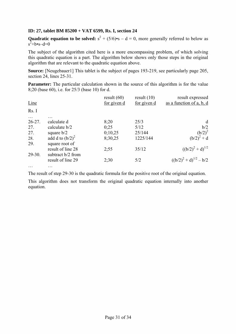
ID: 27, tablet BM 85200 + VAT 6599, Rs. I, section 24 Quadratic equation to be solved: s2 + (5/6)•s – d = 0, more generally referred to below as s2+b•s–d=0





Rs. I … … 26-27. calculate d 8;20 25/3 d 27. calculate b/2 0;25 5/12 b/2 27. square b/2 0;10,25 25/144 (b/2)2 28. add d to (b/2)2 8;30,25 1225/144 (b/2)2 + d 29. square root of result of line 28 2;55 35/12 ((b/2)2 + d)1/2 29-30. subtract b/2 from result of line 29 2;30 5/2 ((b/2)2 + d)1/2 – b/2 … …

The result of step 29-30 is the quadratic formula for the positive root of the original equation.


of 34

ID: 28, tablet BM 85200 + VAT 6599, Rs. I, section 25 Quadratic equation to be solved: s2 – (35/6)•s + c = 0, more generally referred to below as a•s2+b•s+c=0



Parameter: The particular calculation shown in the source of this algorithm is for the value 8;20 (base 60), i.e. for 25/3 (base 10) for c.


Rs. I … … 6-7. calculate c 8;20 25/3 c 7. calculate ⎪b/2⎪ 2;55 35/12 ⎪b/2⎪ 7. square b/2 8;30,25 1225/144 (b/2)2 8i. subtract c from (b/2)2 0;10,25 625/3600 (b/2)2 – c 8ii. square root of result of line 8i 0;25 5/12 ((b/2)2 – c)1/2 9. add ⎪b/2⎪ to result of line 8ii 3;20 10/3 ((b/2)2 – c)1/2 + ⎪b/2⎪ … …



of 34

ID: 29, tablet BM 85200 + VAT 6599, Rs. II, section 30 Quadratic equation to be solved: s2 – (13/12)•s + c = 0, more generally referred to below as a•s2+b•s+c=0


Source: [Neugebauer1] This tablet is the subject of pages 193-219, see particularly pages 207-208, section 30, lines 10-18.

Parameter: The particular calculation shown in the source of this algorithm is for the value 0;17,30 (base 60), i.e. for 7/24 (base 10) for c.


Rs. II … … 12-13. calculate c 0;17,30 7/24 c 14-15. calculate ⎪b⎪ 1;5 13/12 ⎪b⎪ 15. calculate ⎪b/2⎪ 0;32,30 13/24 ⎪b/2⎪ 15. square b/2 0;17,36,15 169/576 (b/2)2 16i. subtract c from (b/2)2 0;0,6,15 1/576 (b/2)2 – c 16ii. square root of result of line 16i 0;2,30 1/24 ((b/2)2 – c)1/2 17. add ⎪b/2⎪ to result of line 16ii 0;35 7/12 ((b/2)2 – c)1/2 + ⎪b/2⎪ … …



of 34

Sources [Berriman] Berriman, A.E., “The Babylonian Quadratic Equation”, The Mathematical Gazette, Vol. 40, October 1956, pp. 185-192.

[Friberg1] Friberg, J., “Mathematik”, S. 531-585 in Edzard, Dietz Otto (Hrsg.), Reallexikon der Assyriologie und Vorderasiatischen Archäologie, Siebter Band, Walter de Gruyter, Berlin, New York, 1987-1990. (Note that although the titles of the book and of the article are in German, the entire text of the article is in English.)

[Friberg2] Friberg, Jöran, A Remarkable Collection of Babylonian Mathematical Texts, Manuscripts in the Schøyen Collection, Cuneiform Texts I, Springer Science+Business Media, New York, 2007.

[Høyrup] Høyrup, Jens, “HERO, PS-HERO, AND NEAR EASTERN PRACTICAL GEOMETRY, An investigation of Metrica, Geometrica, and other treatises”, Roskilde University Centre, Section for philosophy and science studies, 1996 Nr. 5, downloaded from http://akira.ruc.dk/~jensh/Publications/1996%7Bf%7D_Hero.pdf on 2009 January 2.

[Neugebauer1] Neugebauer, O., Mathematische Keilschrift-Texte, Erster Teil, Texte, in Quellen und Studien zur Geschichte der Mathematik Astronomie und Physik, Abteilung A: Quellen, 3. Band, Verlag von Julius Springer, Berlin, 1935.

[Neugebauer2] Neugebauer, O., Mathematische Keilschrift-Texte, Zweiter Teil, Register, Glossar, Nachträge, Tafeln, in Quellen und Studien zur Geschichte der Mathematik Astronomie und Physik, Abteilung A: Quellen, 3. Band, Verlag von Julius Springer, Berlin, 1935.

[Neugebauer3] Neugebauer, O., Mathematische Keilschrift-Texte, Dritter Teil, Ergänzungsheft, in Quellen und Studien zur Geschichte der Mathematik Astronomie und Physik, Abteilung A: Quellen, 3. Band, Verlag von Julius Springer, Berlin, 1937.

[Ritter] Ritter, James, “Babylon –1800”, S. 38-71 in Serres, Michel (Hrsg.), Elemente einer Geschichte der Wissenschaften, Suhrkamp Verlag, Frankfurt am Main, 1994, the German translation of Éléments d’histoire des sciences, Bordas, Paris, 1989.

http://akira.ruc.dk/~jensh/Publications/1996%7Bf%7D_Hero.pdf�

Note on Transformations of Quadratic Equations in Algorithms in Mathematical Cuneiform Texts

Documents

Transcript of Note on Transformations of Quadratic Equations in Algorithms in Mathematical Cuneiform Texts