Nonlinear Finite Element Analysis of Marine and Offshore ...

Guidance Notes on

Nonlinear Finite Element Analysis of Marineand Offshore Structures

January 2021

GUIDANCE NOTES ON

NONLINEAR FINITE ELEMENT ANALYSIS OF MARINEAND OFFSHORE STRUCTURESJANUARY 2021

American Bureau of ShippingIncorporated by Act of Legislature ofthe State of New York 1862

© 2021 American Bureau of Shipping. All rights reserved.ABS Plaza1701 City Plaza DriveSpring, TX 77389 USA

Foreword (2021)With the continuous increase in the size and complexity of marine and offshore structures, new andinnovative design concepts are constantly being envisaged by engineers. With the development ofpowerful computers, more and more engineers turn to advance nonlinear numerical simulation tools inorder to better understand complex engineering processes of new structural concepts that may not beadequately covered by the current Rules and standards. Also, advanced nonlinear numerical tools arewidely used in situations where a structural engineer wants to apply more advanced analysis methods thatgo beyond the standard Rule requirements in order to investigate the behavior of the structure in theinelastic regime, to assess the actual safety margin of the structure, or to gain a better understanding ofalternative load paths, failure mode interactions, and collapse sequences.

Nonlinear finite element analysis (NLFEA) is currently one of the most advanced structural analysisapproaches. It takes into account various sources of nonlinearity such as material, geometry, and boundarycondition nonlinearities such as contact. NLFEA has been developed over the last 60 years and isconsidered mature enough to be applied in daily structural design and analysis. However, the application ofNLFEA is still challenging because many technical aspects need to be carefully considered. Nonlinearanalysis solutions can be non-unique, convergence is not always obtained, and there is often nomathematical error estimation available. While NLFEA is a powerful numerical analysis tool, improperapplication can yield unreliable and inconsistent results.

These Guidance Notes address the main technical aspects of using NLFEA and provide the best practicesand general recommendations for achieving more reliable results when analyzing yielding and plasticdeformations, buckling, ductile static fracture, and dynamic low-cycle fatigue fracture of marine andoffshore structures made of steel. Application examples included in these Guidance Notes are structuralcollapse analysis of a stiffened panel, hull-girder ultimate strength calculations in intact and damagedconditions, dynamic analysis of a container stacks, and impact analysis of a stiffened panel.

The objective of this document is to provide guidance for using NLFEA for cases that are not covered bythe ABS Rules and Guides, or for those involving novel structural designs and loading situations whereNLFEA may provide a better insight into the adequacy of a proposed design.

Additional considerations may be needed for some specific cases, especially when a novel design orapplication is being evaluated. In case of any doubt about the application of these Guidance Notes, ABSshould be consulted.

The January 2021 edition updates the examples in Appendix 1.

These Guidance Notes become effective on the first day of the month of publication.

Users are advised to check periodically on the ABS website www.eagle.org to verify that this version ofthese Guidance Notes is the most current.

We welcome your feedback. Comments or suggestions can be sent electronically by email [email protected].

Terms of Use

The information presented herein is intended solely to assist the reader in the methodologies and/ortechniques discussed. These Guidance Notes do not and cannot replace the analysis and/or advice of aqualified professional. It is the responsibility of the reader to perform their own assessment and obtainprofessional advice. Information contained herein is considered to be pertinent at the time of publicationbut may be invalidated as a result of subsequent legislations, regulations, standards, methods, and/or moreupdated information and the reader assumes full responsibility for compliance. Where there is a conflictbetween this document and the applicable ABS Rules and Guides, the latter will govern. This publicationmay not be copied or redistributed in part or in whole without prior written consent from ABS.

ABS GUIDANCE NOTES ON NONLINEAR FINITE ELEMENT ANALYSIS OF MARINE AND OFFSHORESTRUCTURES • 2021

ii

CONTENTS

SECTION 1 Introduction.......................................................................................... 81 General...........................................................................................8

1.1 Principles of Structural Design Evaluation.........................81.2 Application of NLFEA.......................................................101.3 Types of Structural Failures............................................. 11

2 Scope and Overview of these Guidance Notes............................133 Associated ABS Documents.........................................................144 Abbreviations................................................................................145 Definitions.....................................................................................156 Symbols........................................................................................18

FIGURE 1 Load-Displacement Curve of a Typical Structure...................9FIGURE 2 Partial Safety Factors for LSD Approach............................. 10FIGURE 3 Load-Displacement Curves for Large Plasticity and

Buckling ...............................................................................13

SECTION 2 Sources of Structural Nonlinearity...................................................221 General.........................................................................................222 Geometric Nonlinearity................................................................. 22

2.1 Bifurcation Buckling (Instability).......................................222.2 Large Displacements....................................................... 222.3 Snap-Through Problem................................................... 23

3 Material Nonlinearity.....................................................................244 Boundary Condition Nonlinearity.................................................. 25

FIGURE 1 Load-Displacement Curves for Bifurcation Buckling of aRigid Beam...........................................................................23

FIGURE 2 Load-Displacement Curves for Large Deflection of anElastic System......................................................................24

FIGURE 3 Load-Displacement Curves for Snap-Through of anElastic System......................................................................24

GUIDANCE NOTES ON

NONLINEAR FINITE ELEMENT ANALYSIS OF MARINEAND OFFSHORE STRUCTURES


iii

FIGURE 4 Material Nonlinearity – Elastic-Perfectly Plastic Material..... 25

SECTION 3 Main Aspects of NLFEA.................................................................... 261 General.........................................................................................262 Incremental-Iterative Solution Process.........................................263 Iteration Algorithms.......................................................................27

3.1 Newton-Raphson Algorithms........................................... 283.2 Arc Length (Riks) Algorithm.............................................283.3 Choice of the Iteration Algorithm..................................... 28

4 Numerical Stabilization................................................................. 295 Analysis Type................................................................................30

5.1 Static Analysis................................................................. 305.2 Dynamic Analysis............................................................ 305.3 Quasi-Static Analysis.......................................................34

6 Model Extent.................................................................................357 Loading Approach.........................................................................36

7.1 Displacement Control...................................................... 377.2 Load Control.................................................................... 38

8 Boundary Conditions.................................................................... 389 Material Model.............................................................................. 38

9.1 Yield Condition.................................................................399.2 Flow Rule.........................................................................409.3 Hardening Rule................................................................409.4 Stress-Strain Curves (Flow Curves)................................ 449.5 Strain-Rate Effects...........................................................47

10 Geometric Imperfections...............................................................5010.1 Imposing Measured Imperfections...................................5010.2 Linear Superposition of Eigenmodes...............................5010.3 Direct Shape Definition.................................................... 5110.4 Deformed Shape from Linear Static Analysis.................. 56

11 Ductile Fracture Modeling.............................................................5612 Contact Modeling..........................................................................58

12.1 Definition of Contact Interface Constitutive Properties.... 5812.2 Definition of Contact Pairs............................................... 5812.3 Initial Overclosures and Rough Surface Geometry......... 5912.4 Contact Stabilization........................................................ 59

13 Mesh Quality and Size..................................................................5914 Element Choice............................................................................ 62

14.1 Element Geometric Shape and Order............................. 6214.2 Element Integration Level................................................ 62

TABLE 1 Recommended Unconditionally Stable Time IntegrationSchemes.............................................................................. 32


iv

TABLE 2 Critical Time Increments in Explicit Analysis........................32TABLE 3 Model Extent Recommendations......................................... 36TABLE 4 Material Model Parameters for Common Steel Grades....... 48TABLE 5 Cowper-Symonds Parameters for Small Plastic Strains......49TABLE 6 Recommended Quality Measure Limits for Quadrilateral

Shell and Solid Brick Elements............................................ 60TABLE 7 Mesh Size Recommendations............................................. 60

FIGURE 1 Incremental-Iterative Solution Process................................ 27FIGURE 2 General Load-Displacement Curve......................................29FIGURE 3 Smooth Step Function..........................................................35FIGURE 4 Typical Stress-Strain Curve of Steel.................................... 39FIGURE 5 Von Mises Yield Surface for Plain Stress.............................40FIGURE 6 Kinematic Hardening Model.................................................41FIGURE 7 Isotropic Hardening Model................................................... 41FIGURE 8 Cyclic Hardening and Plastic Shakedown............................43FIGURE 9 Cycle-Dependent Creep and Relaxation..............................43FIGURE 10 True vs. Engineering Flow Curves ...................................... 45FIGURE 11 Schematic Description of the Recommended Material

Model................................................................................... 47FIGURE 12 Design True Flow Curves for Common Marine and

Offshore Steels.................................................................... 48FIGURE 13 Typical Stiffened Panel.........................................................52FIGURE 14 Global Stiffened Panel Imperfections (scale = 50x)............. 52FIGURE 15 Local Imperfections of Plate Between the Stiffeners

(m = 5, scale = 50x) ............................................................ 53FIGURE 16 Local Imperfections of Stiffener Webs (m = 5, scale =

50x)...................................................................................... 54FIGURE 17 Local Tripping Imperfections of Stiffeners (scale = 50x) ..... 55FIGURE 18 Combined Imperfections of Stiffened Panel (scale = 25x) .. 55FIGURE 19 Ductile Fracture Initiation and Evolution...............................57

SECTION 4 Quality Control................................................................................... 641 Choice of NLFEA Program........................................................... 642 General Recommendations for Improving Results Reliability.......643 Validating the Analysis Methodology and Results........................ 654 Documenting the Analysis............................................................ 65

APPENDIX 1 Application Examples........................................................................671 General.........................................................................................672 Ultimate Strength and Post-Collapse Analysis of a Stiffened

Panel.............................................................................................672.1 Geometry, Material, and Initial Imperfections.................. 672.2 Boundary Conditions and Loads......................................68


v

2.3 Mesh Size and Element Type.......................................... 702.4 Analysis Type...................................................................702.5 Results.............................................................................70

3 Ultimate Strength and Post-Collapse Analysis of a Hull Girder....743.1 Geometry, Material, and Initial Imperfections.................. 753.2 Boundary Conditions and Loads......................................753.3 Mesh Size and Element Type.......................................... 763.4 Damage Extent................................................................ 773.5 Analysis Type...................................................................773.6 Results.............................................................................78

4 Time-Domain Analysis of Container Lashing System...................814.1 Container Stack Modeling................................................824.2 Boundary Conditions and Loads......................................844.3 Mesh Size and Element Type.......................................... 864.4 Analysis Type ..................................................................864.5 Results.............................................................................86

5 Indentation of a Stiffened Panel....................................................895.1 Geometry and Material.................................................... 895.2 Boundary Conditions and Loads......................................915.3 Mesh Size and Element Type.......................................... 915.4 Contact Modeling.............................................................915.5 Analysis Type...................................................................915.6 Results.............................................................................92

6 Impact with Ice..............................................................................93

TABLE 1 Model Geometry Parameters...............................................67TABLE 2 Twistlock Clearances........................................................... 82TABLE 3 Model Geometry Parameters...............................................90

FIGURE 1 Stiffened Panel Boundary Conditions.................................. 68FIGURE 2 Kinematic Coupling Between Stiffener Web and Web

Frame ..................................................................................69FIGURE 3 Load-Displacement Curves for Uniaxial Compression.........70FIGURE 4 Kinetic to Internal Energy Ratio for Implicit Quasi-Static

Analyses...............................................................................71FIGURE 5 von Mises Stresses in the Stiffened Panel...........................73FIGURE 6 Load-Displacement Curves for All Three Load Cases.........74FIGURE 7 The Effect of Imperfections on the Load Displacement

Curve....................................................................................74FIGURE 8 CAD Model of the Bulk Carrier.............................................75FIGURE 9 Hull Girder Boundary Conditions..........................................76FIGURE 10 Damage Extent.................................................................... 77FIGURE 11 Moment-Curvature Curves for Intact and Damaged

Conditions............................................................................ 79


vi

FIGURE 12 Interframe Collapse mode of the Intact Bulk Carrier inHogging................................................................................79

FIGURE 13 Collapsed Bulk Carrier with Grounding Damage inHogging................................................................................80

FIGURE 14 Collapsed Bulk Carrier with Collision Damage in Sagging...80FIGURE 15 Kinetic to Internal Energy Ratios..........................................81FIGURE 16 Comparison Between Linear and Nonlinear FEA................ 81FIGURE 17 Nonlinear Behavior of Twistlocks......................................... 83FIGURE 18 Nonlinear Behavior of Lashing Rods ...................................84FIGURE 19 Container Stack Modeling....................................................85FIGURE 20 Time History of Applied Roll Motion at COR........................ 85FIGURE 21 Maximum Twistlock Tension (TT) ........................................87FIGURE 22 Maximum Corner Post Compression (CPC)........................ 87FIGURE 23 Maximum Lashing Rod Tension (LRT) ................................88FIGURE 24 Relative Transverse Deformation of the Stack.....................89FIGURE 25 Model Geometry and Boundary Conditions......................... 90FIGURE 26 Equivalent Plastic Strain Distribution on a Punctured

Stiffened Panel.....................................................................92FIGURE 27 Absorbed Energy Over Time................................................93

APPENDIX 2 Tabulated True Flow Curves............................................................. 94TABLE 1 Steel Grades MS, HS32, HS36............................................94TABLE 2 Steel Grades HS40, HS43, HS47........................................ 95TABLE 3 Steel Grades HS51, HS56, HS63........................................ 97TABLE 4 Steel Grades HS70, HS91, HS98........................................ 98

APPENDIX 3 References........................................................................................101


vii

S E C T I O N 1Introduction

1 GeneralThe stiffness of a discretized structure in a numerical analysis is characterized by its stiffness matrix K.When the structure is in static equilibrium, K relates the vector of external nodal loads, f , to the vector ofnodal displacements, u, as follows:f = Ku .............................................................................................................................................. (1.1)

A structure is said to be nonlinear whenever its stiffness changes with changing loads. The stiffness matrixK can be a function of the structure’s geometric and material properties and change continuously as theapplied load f changes. This requires an incremental and iterative solution of the governing equations ofthe nonlinear system.

Most marine and offshore structures exhibit nonlinear behavior prior to reaching their maximum loadbearing capacity (ultimate strength) after which a progressive collapse and total failure occur. Whenanalyzing various structures, including marine and offshore structures, it is common to plot the relationshipbetween a dominant load acting on the structure and the appropriately chosen measure of the structure’sdeflection (e.g., a hull girder vertical bending moment plotted against a hull girder curvature or acompressive force on the stiffened panel plotted against an average axial displacement of the loaded edgeof the panel in the direction of the applied load). These curves are usually called the load-displacement (P-Δ) or load-shortening curves.

An example of a P-Δ curve is shown in Section 1, Figure 1 for a typical structure exhibiting nonlinearbehavior. Initial response of the structure to the applied load is usually linear up to the proportionality limitwith a constant stiffness matrix K. If the load is increased even further, the structure begins to behave in anonlinear manner due to changes in K. At the point of ultimate strength (largest maxima in the load-displacement curve), the structure reaches its maximum load bearing capacity. At this point, any increasein the applied load will lead to an accelerated response of the structure, as the static equilibrium can nolonger be established.

Nonlinear finite element analysis (NLFEA) is an advanced, robust, and widely used numerical procedurefor analyzing structural problems involving nonlinearities and will be discussed in detail in Section 3.

1.1 Principles of Structural Design EvaluationA marine or offshore structure needs to withstand various static and dynamic loads throughout its entiredesign life. Rules and standards for marine and offshore structures usually rely on the following threestructural design evaluation principles [1]:

1) Working Stress Design (WSD) where the calculated working stress in a structural component doesnot exceed a fraction of the yield stress of the material.


8

2) Critical Buckling Strength Design (CBSD) where the calculated stress in components susceptibleto buckling does not exceed the critical buckling stress which is usually equal to the elasticbuckling stress corrected by a factor that considers plasticity.

3) Limit State Design (LSD) where a reliability theory is used to calculate the actual safety margin ofthe structure subjected to extreme loads. The limit state is defined as the state of the structurebeyond which it is no longer fit for its intended use. Limit states are further categorized as follows[1]:

a) Ultimate Limit State (ULS) represents the state of a structure at which the maximum loadcarrying capacity is reached when the structure is subjected to extreme loads.

b) Accidental Limit State (ALS) represents a state of the structure at which the maximumload-carrying capacity of the structure is reached when the structure is subjected toaccidental loads such as loads due to explosion, collision, and grounding.

c) Fatigue Limit State (FLS) represents the state of a structure at which the maximumcapacity of the structure to withstand cyclic loads is reached.

d) Serviceability Limit State (SLS) represents the state of a structure at which the normalfunctional or operational parameter limits are reached (e.g., local deformation limit).

FIGURE 1Load-Displacement Curve of a Typical Structure

Although WSD and CBSD are generally sufficient for many types of vessels, the use of the moresophisticated LSD approach may be justified in certain cases. The LSD approach requires very precisecalculations of both the ultimate capacity of the structure and the extreme loads. An accurate and generalway to assess the reliability of the structure for all relevant failure modes is to characterize all the randomvariables affecting the loads and the structural capacity using their full probability distributions. Reliabilitytheory is then used to calculate the probability of failure of the structure (reliability = 1 – probability offailure).

Frequently, for marine and offshore structures, the full probabilistic limit state approach is not used due tothe lack of statistical data and complexity of the approach. Approximate probabilistic methods are oftenused such as the Safety Index (SI) method and the Partial Safety Factors (PSF) method (see [2] and [1] formore details). The latter is widely adopted in the marine and offshore industries. It uses the established setof deterministic factors (PSFs) which factor up the characteristic load and factor down the characteristicload limit (capacity or resistance) such that the required level of structural safety can be obtainedconsidering the consequence of each failure mode (see Section 1, Figure 2). For loads, the characteristic

Section 1 Introduction 1


9

value implies that there is a small probability of exceeding this value. For load limit, the characteristicvalue implies that there is a small probability of being below this value. The following condition is to besatisfied:γPPC ≤ PL,C/γL ................................................................................................................................ (1.2)

whereγP = PSF accounting for the uncertainty in the calculated loadγL = PSF accounting for the uncertainty in the calculated load limit (capacity or resistance)PC = characteristic loadPL,C = characteristic load limit

FIGURE 2Partial Safety Factors for LSD Approach

The calculation of load characteristic values is outside of the scope of these Guidance Notes. However,when the NLFEA is used to determine the characteristic load limit using the recommendations contained inthese Guidance Notes regarding finite element (FE) model, material model, and analysis parameters, thecalculated load limit may be considered as a characteristic value with a 5% probability that the actual loadlimit is lower than the calculated load limit. The statistical variability of other parameters affecting the loadlimit that are not specified in these Guidance Notes, such as plate thickness, should be considered whencalculating the statistical properties of the characteristic load limit.

1.2 Application of NLFEAWith the increase in computing capacity, and with the NLFEA achieving maturity, its usage by engineersin the marine and offshore industries has grown rapidly. The cases where the NLFEA is most applied are:

i) When the Rules or standards call for the application of LSD approach. In contrast to WSD andCBSD approaches, LSD approach requires the use of a nonlinear analysis to calculate the limitstate of the structure and to assess the actual safety margin against a certain type of failure. Theexamples may include the calculation of hull girder ultimate strength (reference should be made toParts 5A, 5B, 5C, and 5D of the ABS Marine Vessel Rules, as applicable for specific vessel type)in the intact and damaged conditions (residual strength) and the investigation of the collapsesequence of a stiffened panel.



10

ii) When current Rules or standards do not cover a certain aspect of a structural design or for noveldesigns and loading situations where the NLFEA may be used to provide a better insight into theadequacy of a proposed design

iii) When it is necessary to assess the adequacy of the structure following an accident such ascollision, impact with ice, grounding, or explosion

iv) When it is necessary to assess the crashworthiness of a vessel (i.e., the ability of a vessel to absorbthe energy of the collision while protecting its occupants and cargo)

v) For static and dynamic analysis of structures containing members for which the assumption oflinearity does not hold. An example of such a structure is a container stack with twistlocks andlashing rods, which both exhibit nonlinear structural behavior

vi) Whenever a contact between two surfaces or objects needs to be analyzed and whenever frictionneeds to be simulated

vii) When it is necessary to analyze repeated yielding of the structure and the associated low-cyclefatigue

viii) To assess the redundancy of complex structures (i.e., the ability of a structure to shed loads from afailed member to surrounding intact members and to establish alternative load paths)

ix) To assess the interaction of various failure modes and complete collapse sequence of complexstructures

x) To analyze manufacturing or repair processes involving plastic deformations and residual stresses

xi) Multi-physics analysis (fluid-structure interaction – FSI, thermal-structural coupling, etc.)

xii) To gain insights into complex engineering processes otherwise only accessible by experiments

The recommendations and best practices contained within these Guidance Notes may be applied in theNLFEA of all types of limit states (ULS, ALS, FLS, SLS).

1.3 Types of Structural FailuresThe objective of the LSD approach is to find the loads that cause structural failure at the local memberlevel, or at the global level involving the overall collapse of the entire structure. Since most marine andoffshore structures behave nonlinearly before reaching the ultimate state, LSD may require the use ofNLFEA. Nonlinearities may come from the geometry of the structure, its material, boundary conditions, orfrom the combination of these factors. For structures made of steel, such as marine and offshore structures,the most common and basic types of failure are [2]:

i) Large local plasticity

ii) Buckling (bifurcation or nonbifurcation)

iii) Fracture

● Static (ductile and brittle)

● Dynamic (high-cycle and low-cycle fatigue)

Usually, the failure of a structural component, or the entire structure, involves a combination of the abovebasic failure types. The typical load-displacement curves for members failing due to large local plasticityand buckling are shown in Section 1, Figure 3.

1.3.1 Large Local PlasticityLarge local plasticity is the dominant failure mode in sturdy members which are not susceptible tobuckling. After the proportionality limit has been reached, the growth of the local plastic regionsgradually decreases the stiffness of the structure represented by the slope of the load-displacementcurve. As the stiffness becomes very small, the deflection starts to rapidly increase (see Section 1,



11

Figure 3a). There may not be a well-defined failure point, and the failure load is usually defined asthe load at which the deflection of the structure starts to increase rapidly.

1.3.2 Bifurcation BucklingBuckling, or instability, occurs in slender members under axial or in-plane compressive loads.Bifurcation (branching) buckling is an idealized model assuming a perfect structure without anygeometric or load eccentricities and without any local imperfections or residual stresses. Underthese assumptions, there will be no deflection of the member in any direction other than thedirection of the applied load until a load reaches a certain critical value. After this point, called thebifurcation point, multiple solutions may exist as the load-displacement path branches. Themember’s lateral deflection may stay at zero (unstable solution) or may start to rapidly increase indifferent directions without any increase in the axial load (stable solutions) as seen in Section 1,Figure 3b for an idealized beam.

The bifurcation buckling model is appropriate for many actual slender members, such as beamsand pillars with initial eccentricities and imperfections, where the lateral deflection is very smallprior to the onset of buckling (see Section 1, Figure 3b). The initial load and geometriceccentricities and imperfections determine to which side the member will buckle. Slenderstiffened panels and plates may have some reserve strength (positive stiffness) after the initialbifurcation buckling, as illustrated in Section 1, Figure 3c.

1.3.3 Nonbifurcation BucklingNonbifurcation buckling occurs when the initial deflection of the member increases with theapplied axial or in-plane compressive loads and progressively weakens the structure from thebeginning of load application. Nonbifurcation buckling usually occurs in beams, pillars, plates,and stiffened panels with significant lateral load in combination with in-plane and axialcompressive loads. Due to the coupling between the in-plane or axial loads and the lateraldeflection of the member, the structural response is nonlinear from the beginning of loadapplication. Similarly to large local plasticity, there is no clear onset of buckling or maxima in theload-displacement curve (see Section 1, Figure 3d). Instead, the member is considered to havefailed when a limit value of the deflection has been reached.



12

FIGURE 3Load-Displacement Curves for Large Plasticity and Buckling

1.3.4 Static FractureA static fracture is the rupture of a structural component under the action of static loads. Forductile materials, such as typical steel grades used for marine and offshore structures, significantplastic deformation will occur before static fracture, giving sufficient warning of the imminentfailure. On the other hand, brittle materials do not exhibit large plastic deformations before staticfracture. Steels may become brittle at very low temperatures, depending mainly on their chemicalcomposition. However, steel grades used for marine and offshore structures are engineered to havesufficient ductility, even at low temperatures.

1.3.5 High-cycle and Low-cycle FatigueHigh-cycle fatigue failure occurs when many cycles of moderate dynamic loads are applied to thestructure causing crack initiation and growth to the point where fracture occurs. High-cycle fatigueis governed by the elastic stress range and is analyzed using a linear damage accumulation lawcalled Miner’s Rule. On the other hand, low-cycle fatigue occurs when the structure is subjected toa relatively low number of large dynamic load cycles causing plastic deformations. Low-cyclefatigue is governed by the strain range [3] (strain-based approach to fatigue).

2 Scope and Overview of these Guidance NotesThe objective of these Guidance Notes is to provide the best practices and general recommendations foranalyzing marine and offshore structures using NLFEA. The main technical aspects of NLFEA areaddressed in these Guidance Notes to help the reader to better understand and evaluate the analysis resultsand to aid in troubleshooting possible issues with solution convergence.

These Guidance Notes cover:

● Different sources of structural nonlinearities (see Section 2)



13

● Main technical aspects of NLFEA, such as analysis type, iterative algorithm, time-domain integration,model extent, mesh size, element type, boundary conditions, load application, geometricimperfections, contact, numerical solution stabilization, etc. (see Section 3)

● Quality control (see Section 4)

● Application examples (see Appendix 1)

The recommendations of these Guidance Notes for using NLFEA are applicable to marine and offshorestructures made of steel. All types of structural failures listed in 1/1.3 are covered except for brittle failureand high-cycle fatigue. Brittle failure rarely occurs in marine and offshore structures due to high qualitycontrol of the steel manufacturing and construction processes. Linear high-cycle fatigue analysis procedureand the associated acceptance criteria may be found in ABS Guide for Spectral-Based Fatigue Analysis forVessels and ABS Guide for Spectral-Based Fatigue Analysis for Floating Production, Storage andOffloading (FPSO) Installations.

Design loads and acceptance criteria for NLFEA results regarding various failure modes may be found inABS Rules or other applicable Standards.

3 Associated ABS Documents● ABS Rules for Building and Classing Marine Vessels (Marine Vessel Rules)

● ABS Guide for Certification of Container Securing Systems

● ABS Guide for Spectral-Based Fatigue Analysis for Vessels

● ABS Guide for Spectral-Based Fatigue Analysis for Floating Production, Storage and Offloading(FPSO) Installations

● ABS Guidance Notes on Accidental Load Analysis and Design for Offshore Structures

● ABS Guidance Notes on Ice Class

4 AbbreviationsABS : American Bureau of Shipping

ALS : Accidental Limit State

CAD : Computer Aided Design

CBSD : Critical Buckling Strength Design

COR : Center of Roll

CPC : Corner Post Compression

DOF : Degree of Freedom

FAT : Fully Automatic Twistlock

FE : Finite Element

FEA : Finite Element Analysis

FLS : Fatigue Limit State

FPSO : Floating Production, Storage and Offloading

FSI : Fluid-Structure Interaction



14

HHT : Hilber-Hughes-Taylor

HS : Higher-Strength Steel

ISO : International Organization for Standardization

ISSC : International Ship and Offshore Structures Congress

LRT : Lashing Rod Tension

LSD : Limit State Design

MPC : Multi Point Constraint

MS : Mild Steel (Ordinary-Strength Steel)

NLFEA : Nonlinear Finite Element Analysis

N-R : Newton-Raphson

PSF : Partial Safety Factors

SAT : Semi-Automatic Twistlock

SI : Safety Index

SLS : Serviceability Limit State

TT : Twistlock Tension

ULS : Ultimate Limit State

WSD : Working Stress Design

5 DefinitionsAccidental Limit State. State of a structure at which the maximum load-carrying capacity of the structure isreached when the structure is subjected to accidental loads.

Backstress. Stress tensor by which the yield surface shifts according to the kinematic hardening model.

Bauschinger Effect. Asymmetry of yield stress in tension and subsequent compression of the materialcaused by the shifting of the yield surface in one direction.

Bifurcation Buckling. Idealized model assuming no eccentricities in structure or loads where there is noresponse in the buckling mode until a critical buckling load is reached. At that point, the solution bifurcates(branches) into multiple load-displacement paths.

Characteristic Value of Load or Load Limit. Load design value with a certain small probability of beingexceeded or a load limit design value with a certain small probability of not being exceeded.

Combined Kinematic and Isotropic Hardening. Hardening model which assumes simultaneous isotropicexpansion and kinematic shift of the yield surface.

Contact Pair. A pair of geometric entities or element sets on the same or on different bodies which maypotentially come into contact during the analysis.

Corner Angle. Angle between element edges at a corner.



15

Coulomb Friction Model. Model where friction is proportional to the force acting normal to the contactsurfaces.

Crashworthiness. The ability of a vessel to absorb the energy of the collision while protecting its occupantsand cargo.

Critical Buckling Strength Design . Design principle in which the calculated stress in componentssusceptible to buckling does not exceed the critical buckling stress.

Critical Time Increment (for Explicit Analysis). The maximum size of a time increment allowing for astable and accurate solution. It is approximately equal to the time it takes a stress wave to propagate acrossthe smallest finite element dimension.

Cycle-Dependent Creep. The increase of the mean strain when the material is subjected to biased stresscycles.

Cycle-Dependent Relaxation. The shifting of the mean stress towards zero when the material is subjectedto biased strain cycles.

Cyclic Hardening. Phenomenon where the maximum stress reached in each of the hysteresis loops of asymmetric strain-controlled loading cycle gradually increases.

Displacement Control. Analysis approach in which the displacement application is controlled.

Drilling Stiffness. Rotational stiffness of a shell element about the direction normal to plane of the element.

Element Aspect Ratio. Ratio of maximum to minimum element edge length.

Engineering Stress and Strain. Stress and strain calculated based on the initial cross section and length of atest specimen, respectively.

Explicit Time Integration. Time integration in which the displacements and velocities at the next timeincrement are nonlinear functions of the displacements and velocities at the previous time increments onlyand can be calculated explicitly without the iterative solution process.

Fatigue Limit State. State of a structure at which the maximum capacity of the structure to withstand cyclicloads is reached.

Flow Curve. Uniaxial stress-plastic strain curve that defines the flow rule.

Flow Rule. Relationship between the plastic strain increment and the stress increment once the stress stateis on the yield surface.

Follower Loads. Loads that follow the nodal translation and rotation of the structure.

Geometric Nonlinearity. Type of nonlinearity that occurs in structures that exhibit large displacements androtations such that the applied loads and/or the stiffness of the structure become dependent on thestructure’s geometry.

Hard Contact. Type of pressure-overclosure relationship where the contact pressure is zero when thesurfaces are not in contact and where there is no penetration of one surface into another.

Hardening Rule. Rule that describes how the yield surface evolves when plastic straining occurs.

High-Cycle Fatigue. Many cycles of moderate dynamic loads are applied to the structure causing crackinitiation and growth to the point where fracture occurs.



16

Hourglassing. Numerical issue that is characterized by the occurrence of spurious, zero strain energybending modes of first-order elements with reduced integration.

Implicit Time Integration. Time integration in which the displacements and velocities at the next timeincrement are nonlinear functions of the displacements and velocities at the next and previous timeincrements. It requires an iterative solution process.

Isotropic Hardening. Hardening model which assumes that the yield surface expands equally in alldirections when plastic straining occurs.

Jacobian. Measure of the element’s deviation from an ideal shape.

Kinematic Hardening. Hardening model which assumes that the yield surface does not change in size orshape, but simply shifts in the stress space.

Large Local Plasticity. Growth of the local plastic regions that gradually decreases the stiffness of thestructure.

Limit State Design. Design principle in which the reliability theory is used to calculate the true safetymargin of the structure subjected to extreme loads.

Load Control. Analysis approach in which the load application is controlled.

Load-Displacement Curve. Relationship between a dominant load acting on the structure and theappropriately chosen measure of the structure’s deflection.

Load-Shortening Curve. See “Load-Displacement Curve”.

Low-Cycle Fatigue. Relatively low number of large dynamic load cycles causing plastic deformations andfracture.

Mass Scaling. Artificial increasing of material density in order to increase the critical time incrementduring explicit analysis.

Material Nonlinearity. Nonlinearity stemming from the nonlinear material behavior as characterized by anonlinear uniaxial stress-strain function.

Necking. Localization of strains in a ductile material. In a tensile test of a cylindrical specimen, necking ismanifested as a local reduction of cylinder radius.

Nonbifurcation Buckling. Type of buckling that occurs when the initial deflection of the member increaseswith the applied axial or in-plane compressive loads and progressively weakens the structure from thebeginning of load application.

Numerical Stabilization. Introduction of artificial damping elements at the nodes where the ratio ofdisplacement increments to load increments is very high.

Partial Safety Factors. Deterministic factors which factor up the characteristic load and factor down thecharacteristic load limit of a structure such that the required level of structural safety can be obtainedconsidering the consequence of each failure mode.

Penalty Method. Numerical method used to enforce the contact pressure-overclosure relationship.

Plastic Shakedown. Stabilization of the cyclic hardening over a certain number of cycles.

Ratchetting. See “Cycle-Dependent Creep”.



17

Reversed Mass Scaling. Technique which consists of reducing the material density in order to minimize theinertial effects during the quasi-static analysis.

Safety Index. Inverse of the coefficient of variation of the margin between the actual load and the load limitvalue (capacity). It determines the degree of safety of the structure.

Selective Subcycling. Technique used during the explicit analysis to reduce the total computation time. It isused when a small number of elements with a very small critical time increment govern the totalcomputation time. Instead of integrating all the elements with this very small time increment, theremaining elements are integrated with their significantly larger critical time increment.

Serviceability Limit State. State of a structure at which the normal functional or operational parameterlimits are reached.

Shear Locking. Excessive stiffness in bending of first-order fully integrated finite elements caused byspurious shear strains.

Skewness Angle. Difference between the right angle and the smallest angle between intersecting elementmid-lines.

Smooth Step. Mathematical function that gradually increases the load application rate from zero to amaximum value and then gradually decreases the load application rate to zero towards the end of theanalysis.

Snap-Back. Unstable structural response that occurs when the displacement is gradually incremented.

Snap-Through. Unstable structural response that occurs when a structure suddenly assumes anotherconfiguration under the action of an external load.

Static Fracture. Rupture of a structural component under the action of static loads.

True Stress and Strain. Stress and strain calculated based on a specimen’s instantaneous cross-section andinstantaneous strain increment, respectively.

Ultimate Limit State. State of a structure at which the maximum load carrying capacity is reached when thestructure is subjected to extreme loads.

Ultimate Strength. Maximum load-bearing capacity of the structure.

Volumetric Locking. Excessive stiffness of fully integrated elements to deformations that cause no changein the volume of the element. Volumetric locking is caused by spurious pressure stresses.

Warping Angle. Out-of-plane element warping.

Working Stress Design. Design principle in which the calculated working stress in a structural componentdoes not exceed a fraction of the yield stress of the material.

Yield Condition. Combination of stresses in a certain structural component when the material starts toyield.

Yield Surface. Mathematical function describing the yield condition.

6 Symbolsa Distance between the strong stiffened panel supports in the x direction

A Overall stiffened panel length



18

b Spacing of stiffened panel stiffeners; plate breadth; grounding damage breadthbf Breadth of flangeB Total breadth of the stiffened panel in the y directionc Dilatational wave speedC Damping matrixC Parameter of the Cowper-Symonds modeld Collision damage breadthd1,d2,d3,d4,d5 Parameters of the Johnson-Cook ductile fracture criteriaE Modulus of elasticityf Functionf Vector of external nodal loadsF ForceFx Compressive load in x directionFy Compressive load in y directionℎ Collision or grounding damage heightℎw Height of the stiffener webH Half-length of one structural fold of a thin plateK Stiffness matrixK Constant of the power-hardening true stress-strain relationshipKt Tangent stiffnessL Finite element lengthm Number of half-waves between the stiffened panel strong supports in the x directionM Mass matrixn Strain-hardening exponent of the power-hardening true stress-strain relationshipns Number of stiffeners between strong longitudinal supportsP LoadPC Characteristic loadPL .C Characteristic load limitq Parameter of the Cowper-Symonds modelr Radius of the indenterR Residual loadRxi–j Rotation around the x axis of edge connecting corners i and jRyi Rotation around the y axis of corner iRyi–j Rotation around the y axis of edge connecting corners i and jRzi Rotation around the z axis of corner iRzi–j Rotation around the z axis of edge connecting corners i and j



19

S Current cross-sectional area of the test specimenS0 Initial cross-sectional area of the test specimenS(t) Smooth step functiont Time or plate thicknesstf Thickness of flangetp Thickness of platetw Thickness of webT Time period over which the full load is applied such that S(T) =1u Vector of nodal displacementsup Equivalent plastic displacementupf Equivalent plastic displacement at fractureUxi Translation in the x direction of corner iUxi–j Translation in the x direction of edge connecting corners i and jUyi Translation in the y direction of corner iUzi Translation in the z direction of corner iV0 Initial speed of the dynamic loadw Vertical displacementα Backstress tensorα Parameter of Hilber-Hughes-Taylor implicit time integration schemeβ Parameter of Hilber-Hughes-Taylor implicit time integration schemeγ Parameter of Hilber-Hughes-Taylor implicit time integration schemeγL PSF accounting for the uncertainty in the calculated load limitγP PSF accounting for the uncertainty in the calculated loadδ Average displacement of the structural elementδy, flange Transverse displacements of the stiffener flange nodesδy,web Transverse displacements of the stiffener web nodesδz, flange Vertical displacements of the stiffener flange nodesδz, panel Vertical displacement of the stiffened panel nodesδz, plate Vertical displacement of the stiffened panel plate nodesδz,web Vertical displacements of the stiffener web nodes∆ DisplacementΔP Load incrementε True strainε Strain rateεcf Critical fracture strain



20

εel Elastic portion of the true strainεeng Engineering strainεijp Components of the plastic strain rate tensorεp True plastic strainεp Equivalent plastic strainεsℎ, eng Engineering strain at the start of the strain hardening regionεu, eng Engineering strain at the point where ultimate engineering stress is reachedεy, eng Engineering strain at the onset of yieldingv Poisson ratioρ Densityσ True stressσ1,σ2,σ3 Principal stresses in the three orthogonal directionsσY Yield stressσY, eng Engineering yield stressσU, eng Engineering ultimate stressσ(ε) Static true flow curveσ(ε)dyn Dynamic true flow curveφ Rotation angle



21

S E C T I O N 2Sources of Structural Nonlinearity

1 GeneralThere are three main sources of nonlinearity in solid mechanics:

1) Geometric nonlinearity

2) Material nonlinearity

3) Boundary condition nonlinearity

Since the solution methods of the NLFEA should be adjusted according to the type of nonlinearity, allthree sources of nonlinearity are described separately in the next Subsections.

2 Geometric NonlinearityGeometric nonlinearity occurs in structures such as beams and shells that exhibit large displacements androtations such that the applied loads and/or the stiffness of the structure become dependent on thestructure’s instantaneous geometry. A few classical examples of geometric nonlinearity are given in thefollowing Paragraphs, and more details can be found in [4].

2.1 Bifurcation Buckling (Instability)A simple example features an idealized rigid beam supported by an elastic rotational spring and loadedwith an axial compression force, F, without any eccentricities, as shown in Section 2, Figure 1. After theforce reaches a critical value that depends on the length of the beam and the stiffness of the rotationalspring, the solution of the nonlinear problem starts to bifurcate (branch). This critical point is called thebifurcation point, after which three different solutions are possible: an unstable trivial solution in whichthere is no rotation of the beam, and two stable symmetric solutions with either positive or negativerotation of the beam, , as shown in Section 2, Figure 1. Initial eccentricities in the geometry or the load,that are common in structures, will determine which of the two stable solutions is followed as thecompressive force is increased.

2.2 Large DisplacementsAnother example of geometric nonlinearity is shown in Section 2, Figure 2, where a system of twoconnected elastic rods is subjected to large displacements by a force, F, acting at their connection point. Asthe rods are stretched, the axial forces in the rods grow and progressively resist the applied vertical force asthe angle of the rods with respect to the horizontal increases. Therefore, the force needed for anincremental increase in the vertical displacement, w, grows with the vertical displacement, as shown withthe force-displacement curve in Section 2, Figure 2.


22

2.3 Snap-Through ProblemThe snap-through problem occurs when a structure suddenly assumes another configuration under theaction of an external load. An example of such nonlinear behavior is shown in Section 2, Figure 3. Thisexample is very similar to the example in 2/2.2, but in this case, the elastic rods form an isosceles trianglewith the horizontal in their initial unloaded configuration. The force displacement curve for this problem isalso shown in Section 2, Figure 3. As the force, F, reaches a critical value at point A, an instability occurs,and the structure instantaneously snaps through from one equilibrium state at point A to anotherequilibrium state at point B.

FIGURE 1Load-Displacement Curves for Bifurcation Buckling of a Rigid Beam

Section 2 Sources of Structural Nonlinearity 2


23

FIGURE 2Load-Displacement Curves for Large Deflection of an Elastic System

FIGURE 3Load-Displacement Curves for Snap-Through of an Elastic System

3 Material NonlinearityGeometric nonlinearities occur when the structure’s displacements are large. If the strains are large as well,then material nonlinearity may also affect the structure’s behavior. Many materials, including steel, exhibitnonlinear behavior which is characterized by a nonlinear uniaxial stress-strain function. Section 2, Figure 4shows an idealized elastic-perfectly plastic material behavior where the initial slope of the elastic region



24

sharply decreases to zero allowing the material to strain indefinitely with no further increase in stress. Mostreal materials exhibit some strain hardening until the ultimate stress of the material is reached.

Similar to geometric nonlinearity, which can be the cause of structures’ instability (bifurcation buckling,snap-through, snap-back), material nonlinearity can also cause instability in the form of necking, plastichinges, or shear bands.

FIGURE 4Material Nonlinearity – Elastic-Perfectly Plastic Material

4 Boundary Condition NonlinearityBoundary conditions may be the sources of nonlinearity in cases where, for example, two bodies come intocontact with one another or in cases where the loads or load paths depend on the deformation of thestructure. The follower loads that follow the nodal translation and rotation of the structure fall into thelatter category. An example of these follower loads is a liquid pressure that always acts normal to thedeformed surface.



25

S E C T I O N 3Main Aspects of NLFEA

1 GeneralThis Section addresses the following main aspects of the NLFEA:

● Incremental-iterative solution process

● Iteration algorithms

● Numerical stabilization

● Analysis type

● Model extent

● Loading approach

● Boundary conditions

● Material model

● Geometric imperfections

● Ductile fracture modeling

● Contact modeling

● Mesh quality and size

● Element choice

The following Subsections discuss each of these aspects and provide general guidance andrecommendations.

2 Incremental-Iterative Solution ProcessIn a linear analysis, the solution is calculated directly in one step by solving a system of linear equations.However, in order to trace the solution path in a nonlinear analysis, the load (or prescribed displacement)should be divided into a series of smaller increments. For each load increment equilibrium, a solution isfound by performing several iterations, each of which is computationally comparable to a solution of alinear system. Therefore, nonlinear analysis may be computationally much more demanding compared tothe linear analysis. Section 3, Figure 1 shows the basic incremental-iterative approach to solving nonlinearproblems with two load increments (ΔP1 and ΔP2) and three iterations within each of the two loadincrements.

In most commercial NLFEA programs, the load is prescribed as a function of time. In a static analysis, thetime is usually specified from zero to one, and it does not have a physical meaning. It only tells theprogram how to increment the load from its initial value at time equal to zero to its final value at time


26

equal to one. In this case, each load increment is specified as a fraction of total time over which the load isprescribed.

Load incrementation in many commercial NLFEA programs is controlled automatically by the software inorder to reduce the computation time, although manual control is also available. For most nonlinearproblems, automatic increment control is sufficient and recommended. The user should only specify thesize of the first load increment. A reasonable value of the initial load increment should be provided. Avalue that is too large or too small will require significant subsequent reductions or growth of the loadincrement resulting in wasted computing effort. Prior knowledge or experience related to similar problemscan aid in selecting a reasonable initial increment. Otherwise a value of 10% of the maximum load may beused. The manual increment control should only be used in rare circumstances when convergence cannotbe achieved by any other means. Also, iteration algorithms have a finite radius of convergence, whichmeans that a load increment that is too large may prevent the nonlinear solver from converging to asolution.

FIGURE 1Incremental-Iterative Solution Process

At each load increment, the nonlinear solver begins the iterative process to find the equilibrium solutionand stops when convergence is achieved as judged by the tolerances specified in the solver. The solution ateach load increment is said to be converged when certain residuals are below the specified tolerances.Usually, the iterative solver monitors the difference between the external and internal loads, called theresidual load, R (see Section 3, Figure 1), and stops when R falls below a small tolerance value that is setas a solver default or edited by the user. There may be other convergence checks specific to eachimplementation of the iterative solver. It is not recommended to change the default tolerance values for theconvergence checks unless the analyst has an in-depth knowledge of the nonlinear solver and how thechanges may affect the solution accuracy. Any such changes should be well documented and supported.

3 Iteration AlgorithmsWhen the stiffness matrix is dependent on either the displacement vector or the load vector, or both, theproblem is nonlinear and will require an iterative algorithm to solve it. The three main iteration algorithmsare:

1) Newton-Raphson (N-R) Algorithm for static or dynamic implicit analysis

2) Modified N-R (Quasi N-R) Algorithm for static or dynamic implicit analysis

Section 3 Main Aspects of NLFEA 3


27

3) Arc Length (Riks) for static analysis only

3.1 Newton-Raphson AlgorithmsThe N-R algorithm [2] updates the tangent stiffness, Kt (see Section 3, Figure 1) at each iteration in orderto find progressively better estimates of the equilibrium solution with progressively smaller residual loadsR.

The modified N-R algorithm is similar to the N-R algorithm but uses a constant tangent stiffness for all theiterations within a particular load increment. Not having to calculate Kt at each iteration considerablyreduces the computational effort. However, the modified N-R method usually requires more iterations toachieve comparable accuracy as the N-R method, thus offsetting the efficiency gain.

3.2 Arc Length (Riks) AlgorithmThe Arc Length algorithm [5], also known as the Riks algorithm [6] controls both the load incrementationprocess and the iteration process used to eliminate the unbalanced loads. This method considers the loadincrement, ΔP, as an additional unknown and solves simultaneously for loads and displacements. Theprogress of the solution is measured by the “arc length” along the static load-displacement curve. Since theload is a part of the solution and not prescribed using a certain function, it is possible to analyze globalpost-ultimate strength or post-buckling behavior. In order to use the Arc Length method, all loads acting onthe structure need to be proportional, meaning they can all be scaled with a single parameter.

The Arc-Length algorithm is not well suited for analyzing bifurcation buckling problems. Usually, whenusing the Arc-Length algorithm, initial imperfections should be applied to the structure (see 3/10). In thatcase, there will be a continuous response by the structure before the critical buckling load is reached, andbifurcation buckling will be avoided.

3.3 Choice of the Iteration AlgorithmThe choice of the iteration algorithm will depend upon the analysis type (see 3/5), load control approach(see 3/7), and the expected load-displacement behavior of the structure. Section 3, Figure 2 shows a verygeneral load-displacement curve of a highly nonlinear structure experiencing snap-through (see 2/2.3) andsnap-back behavior. As opposed to snap-through behavior that occurs when the load is graduallyincremented (load control approach), snap-back behavior occurs when the displacement is graduallyincremented (displacement control approach). At point C, called the turning point, the structure may snapback to point D as illustrated in Section 3, Figure 2.



28

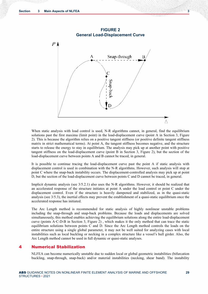
FIGURE 2General Load-Displacement Curve

When static analysis with load control is used, N-R algorithms cannot, in general, find the equilibriumsolutions past the first maxima (limit point) in the load-displacement curve (point A in Section 3, Figure2). This is because the algorithm relies on a positive tangent stiffness (or positive definite tangent stiffnessmatrix in strict mathematical terms). At point A, the tangent stiffness becomes negative, and the structurestarts to release the energy to stay in equilibrium. The analysis may pick up at another point with positivetangent stiffness on the load-displacement curve (point B in Section 3, Figure 2), but the section of theload-displacement curve between points A and B cannot be traced, in general.

It is possible to continue tracing the load-displacement curve past the point A if static analysis withdisplacement control is used in combination with the N-R algorithms. However, such analysis will stop atpoint C where the snap-back instability occurs. The displacement-controlled analysis may pick up at pointD, but the section of the load-displacement curve between points C and D cannot be traced, in general.

Implicit dynamic analysis (see 3/5.2.1) also uses the N-R algorithms. However, it should be realized thatan accelerated response of the structure initiates at point A under the load control or point C under thedisplacement control. Even if the structure is heavily dampened and stabilized, as in the quasi-staticanalysis (see 3/5.3), the inertial effects may prevent the establishment of a quasi-static equilibrium once theaccelerated response has initiated.

The Arc Length method is recommended for static analysis of highly nonlinear unstable problemsincluding the snap-through and snap-back problems. Because the loads and displacements are solvedsimultaneously, this method enables achieving the equilibrium solutions along the entire load-displacementcurve (points A‑C-D-B in Section 3, Figure 2) , which makes it the only method that can trace the staticequilibrium solutions between points C and D. Since the Arc Length method controls the loads on theentire structure using a single global parameter, it may not be well suited for analyzing cases with localinstabilities such as local buckling or necking in a complex structure like a vessel’s hull girder. Also, theArc Length method cannot be used in full dynamic or quasi-static analyses.

4 Numerical StabilizationNLFEA can become numerically unstable due to sudden local or global geometric instabilities (bifurcationbuckling, snap-through, snap-back) and/or material instabilities (necking, shear band). The instability



29

comes from the fact that the displacements or strains at the onset of instability become very large, eventhough the load increment is kept relatively small. Global instabilities can frequently be assessed using theArc-Length method (see 3/3.2 and 3/3.3). However, the Arc-Length method may not work if theinstabilities are local such that a part of the structure releases the strain energy while the neighboring partsof the structure accumulate it. Such local instabilities often arise in the limit state analysis of complexstructures (e.g., ultimate strength analysis of a hull girder) and must be treated either dynamically (see3/5.2 and 3/5.3) or/and numerically stabilized using artificial damping.

Numerical stabilization is based on the introduction of artificial damping elements at the nodes where theratio of displacement increments to load increments is very high. Numerical stabilization can be used inboth static and dynamic analyses. In a static analysis, damping is proportional to the ratio of the nodaldisplacement increment and the load increment, where the load increment is expressed as a fraction of totaltime. In a dynamic analysis, artificial damping has a physical meaning and is proportional to the nodalvelocity.

The amount of damping needed to stabilize a certain problem is not known in advance. The proper amountof damping will depend on the type of system being analyzed, the analysis type, the mesh size, and theextent of the model. Experience with a similar type of problem and some trial-and-error simulations canhelp determine the right amount of damping. Too much damping can lead to unrealistically stiff structuresand will affect the final static or dynamic equilibrium. Too little damping will not be able to stabilize theproblem.

It is important to verify that, after the problem has been stabilized and the convergence has been achieved,the accumulated stabilization energy is less than 5% of the model’s total strain energy (internal energy) ateach increment of the analysis. The accumulated stabilization energy is readily available as an output inmost commercial NLFEA programs.

Most commercial NLFEA programs offer automatic numerical stabilization of unstable problems. This isthe preferred method of stabilization since the program automatically applies artificial damping only to thenodes with high local velocity, while keeping the accumulated stabilization energy below a user-specifiedsmall fraction (5% is recommended) of the model’s total strain energy at each increment of the analysis.

5 Analysis TypeThe following main analysis types of NLFEA are briefly described in this Subsection:

1) Static analysis

2) Dynamic analysis

3) Quasi-static analysis

5.1 Static AnalysisDuring a static analysis, loads or displacements are applied incrementally. At each load increment, staticequilibrium (Eq. 1.1) is found using an iterative numerical algorithm (e.g., N-R or Arc Length), asdescribed in 3/3.1 and 3/3.2. Inertial effects are not accounted for, as well as time-dependent materialeffects such as creep. However, strain rate effects on material plasticity can be taken into account. Whenthe N-R iteration algorithm is used and local instabilities (local buckling, material necking, etc.) areexpected to occur, numerical stabilization techniques should be applied as in 3/4.

5.2 Dynamic AnalysisNonlinear dynamic analysis uses either implicit (Backward Euler or Hilber-Hughes-Taylor) or explicit(Central Difference) direct time integration schemes to propagate the solution across all time increments.Both integration methods solve the dynamic system of equations:f = Mu+ Cu+Ku ....................................................................................................................... (3.1)



30

whereM = mass matrixC = damping matrixu = vector of time dependent nodal displacements f = vector of time dependent external nodal loads

5.2.1 Implicit Dynamic AnalysisWhen implicit time integration is used, the displacements and velocities at the current time stepare nonlinear functions of the displacements and velocities at the current and previous time steps,thus requiring an iterative solution using the N-R algorithms at each time increment of theanalysis.

The most commonly used implicit time integration scheme is the Hilber-Hughes-Taylor (HHT)[7], which is an extension of the Newmark β-method. Another commonly used scheme is theBackward Euler. All numerical integration schemes introduce some level of artificial (non-physical) numerical damping. The Backward Euler scheme introduces more numerical dampingcompared to the HHT scheme and is usually used when quasi-static analysis (see 3/5.3) isperformed.

The HHT time integration scheme is controlled by three parameters: α, β, and γ. Parameter αvaries in the range – 1 2 ≤ α ≤ 0 and controls the amount of numerical damping. It is highlyrecommended to set the other two parameters as follows:β = 14 1− α 2 > 0 and γ = 12 − α ≥ 12 .............................................................................. (3.2)

This preserves the unconditional stability of the HHT integration scheme for linear problems orlinear portions of nonlinear problems, which means that the time increment in a linear implicitdynamic analysis can be arbitrarily large, and that the converged solution at a given time instantcan be obtained in only one time increment. The same stability characteristics cannot beguaranteed in a nonlinear analysis, but the unconditionally stable HHT scheme in a linear analysiswill also have desirable characteristics in a nonlinear analysis. Section 3, Table 1 shows therecommended time integration schemes and parameter values for various types of implicitdynamic analyses.

HHT with α= 0 is also called the Trapezoidal Rule and has no numerical damping. However, somenumerical damping is always desirable to improve the convergence behavior and reduce the high-frequency solution noise.

Automatic time incrementation is recommended, which allows the implicit solver to minimize thecomputation time while achieving convergence at each time increment.

For transient analyses involving high-frequency vibrations (e.g., whipping of the hull girdercaused by slamming), it is recommended to limit the maximum time increment to 1/100 of thetotal simulated time span or 1/10 of the smallest natural vibration period of interest, whichever issmaller.



31

TABLE 1Recommended Unconditionally Stable Time Integration Schemes

Time Integration Scheme Parameters Damping Typical Applications

α β γ

Backward Euler NA Significant Quasi-static analysis

HHT

0 0.25 0.5 Zero Transient analysis involvingvery high-frequency vibrations

–0.05 0.27563 0.55 Very small Transient analysis involvinghigh-frequency vibrations

–0.41421 0.5 0.91421 Medium Collision analysis−1 3 4 9 5 6 Maximum(for HHT)

Quasi-static analysis

For dynamic analyses involving moderate energy dissipation mechanisms where high-frequencyvibration modes are not of interest (e.g., collision analysis), the maximum time increment shouldbe limited to1 10 of the total simulated time span.

For quasi-static analysis (see 3/5.3), there is no need to use the upper bound for the timeincrement. The automatic time incrementation will use large time increments when possible toachieve maximum computation efficiency.

5.2.2 Explicit Dynamic AnalysisWhen explicit time integration is used, the displacements and velocities at the current time step arenonlinear functions of the displacements and velocities at the previous time steps only and can becalculated explicitly without the iterative solution process. This means that each time increment ofthe explicit method is computationally much more efficient compared to the implicit method.However, the Central Difference integration scheme is conditionally stable, unlike theunconditionally stable implicit time integration schemes (see 3/5.2.1). The size of the critical timeincrement (allowable time increment) in the explicit analysis is approximately equal to the time ittakes a stress wave (dilatational wave) to propagate across the smallest finite element dimension.Section 3, Table 2 shows the critical time increment for explicit dynamic analysis for rod, shell,and solid finite elements.

TABLE 2Critical Time Increments in Explicit Analysis

Finite Element Critical Time Increment Δtc

Rod ∆ tc = Lc = L ρEShell ∆ tc = Lc = L 1− ν2 ρESolid ∆ tc = Lc = L 1 + ν 1− 2ν ρE 1− ν

where



32

L = smallest finite element dimension in the meshc = dilatational wave speedv = Poisson ratioE = modulus of elasticityρ = density

The critical time increment for beam elements is computed in a similar way. However, L is equalto the length of the beam only for the axial deformation mode and is computed differently forbending, shear, and torsion deformation modes. In practice, the critical time increment of the beamelement can be smaller compared to other element types of similar size present in the mesh. Forthat reason, attention should be paid when using beam elements in the explicit dynamic analysis ofmarine and offshore structures.

The critical time increment of the explicit analysis, even without the beam elements, is likely to bemuch smaller compared to the time increment of the implicit analysis. Therefore, the time savedon avoiding iterations can be offset by the large number of required time increments.

In order to reduce the computation time, it is necessary to increase the critical time increment (seeSection 3, Table 2) or to reduce the total simulated time. This can be done using four differenttechniques:

1) Increasing the size L of the smallest element in the mesh by a factor ƒ increases the timeincrement and decreases the computation time by the same factor. The effect can be evenlarger if by increasing L, the number of nodes in the model reduces significantly.Increasing L may decrease the accuracy of the finite element solution.

2) Artificially increasing the material density, ρ, by a factor ƒ2 will reduce the requirednumber of time increments (and the total simulation time) by a factor ƒ. This is calledmass scaling. Increasing the mass density will increase the inertial forces and maysignificantly affect the solution. Therefore, the mass scaling factor ƒ should be chosencarefully. Inertial forces should be monitored during the solution to make sure they do notbecome dominant. For quasi-static problems, kinetic energy of the system should bemonitored to make sure it does not become larger than 5% of the internal strain energy,except at the beginning of the analysis where this ratio may exceed 5% due to very smallstrain energy. In order to minimize the inertial effects, mass scaling can be appliedselectively to only the elements whose critical time increment is below a specified value.This can be accomplished in most commercial NLFEA programs.

3) Artificially speeding up the simulation by increasing the load application rates by a factorƒ will reduce the computation time by the same factor. This has the same effect on thesimulation results as mass scaling and the same precautions should be made in terms ofmonitoring the inertial forces. In addition to this, speeding up the simulation should notbe done if time/rate dependent material behavior is specified in the analysis.

4) In cases where there is a relatively small number of very small elements governing thecritical time increment and where all the other elements in the model are significantlylarger, the total computation time can be considerably reduced if the two groups ofelements are integrated separately using different critical time increments. In that case,the bigger group of larger elements is integrated using a correspondingly larger timeincrement which can significantly speed-up the simulation. This technique is calledselective subcycling.

Due to the large number of time increments needed in the explicit dynamic analysis, the smallnumerical roundoff errors in each time increment can quickly accumulate into a significant error.



33

Therefore, it is strongly suggested to use double precision float numbers when running an explicitanalysis.

5.2.3 Implicit vs. Explicit Dynamic AnalysisBoth implicit and explicit time integration schemes can be used for a wide range of dynamicproblems. In many cases, the choice will not be obvious and will depend on the specifics of theanalyzed system. The following paragraphs present some general guidance.

The computation cost of the explicit analysis depends linearly on the number of elements in themodel. The computation cost of the implicit analysis rises more rapidly with the number ofelements in the model. Therefore, explicit analysis will be computationally very effective for largeproblems, (e.g., ultimate strength analysis of a 2-hold hull girder model or collision analysis oftwo vessels).

The explicit method is usually more efficient than the implicit method for solving highly dynamicand discontinuous events over a short period of time (e.g., impact and explosions).

The explicit method can usually achieve convergence in cases where the implicit method fails,since it does not require iteration.

Although both time integration schemes can be used to solve quasi-static problems (see 3/5.3), aslight preference should be given to the implicit scheme, since it provides more options fordamping the solution and minimizing inertial effects. For example, the inertial effects can beminimized by reducing the material density, which is called reversed mass scaling. This will notimpact the solution time of the implicit scheme, but it will have a detrimental effect on the criticaltime increment of the explicit scheme (see 3/5.2.2). Likewise, increasing the load application timemay not have a big impact on the computational time when implicit analysis is used due to the factthat larger time increments may be used, but it will proportionally increase the computation timeof the explicit analysis where the critical time increment remains unchanged.

5.3 Quasi-Static AnalysisQuasi-static analysis is a dynamic analysis whose purpose is to estimate the static response of the structureby minimizing the inertial effects, which are only introduced to mitigate the unstable behavior of thestructure. It is mainly used when static analysis fails to converge. Examples may include the ultimate andpost-ultimate strength analysis of a hull girder or a collapse analysis of a stiffened panel or a web frame.The maxima (limit point) in the load-displacement curve (point A in Section 3, Figure 2) can be passedusing either load control or displacement control approaches. However, when the structure reaches itsultimate capacity at point A, any further incremental increase in the external load, which can no longer besustained by the structure, will initiate the accelerated response of the structure. At this point, it becomesincreasingly more difficult to dampen and stabilize the structure, and its kinetic energy may quickly growto over 5% of the internal strain energy of the system. At that point, the solution can no longer beconsidered as quasi-static.

There are three ways to minimize the inertia effects and to achieve a quasi-static equilibrium usingdynamic analysis:

1) Loads are applied over a long time period, which increases the number of time increments whenexplicit analysis is used.

2) Density of the structural material is deliberately lowered by an order of magnitude (reversed massscaling). This will have a negative effect on the critical time increment for explicit analysis butwill not affect the implicit analysis.

3) Numerical and/or structural and material damping is used, which also stabilizes the system andimproves convergence.



34

In addition to the above-mentioned ways of minimizing the inertia effects, another useful approach tominimize the inertia effects (especially at the beginning of the analysis when the internal strains in thestructure are small) is to use a smooth step function to apply the loads or displacements. The smooth stepfunction gradually increases the load application rate from zero to a maximum value and then graduallydecreases the load application rate to zero towards the end of the analysis, as can be seen in Section 3,Figure 3.

The mathematical expression for the smooth step function is as follows:S t = tT 2 3− 2 tT 2 . . . . . . . . . . . . . . . . . . . . . . . . . . . . . . . . . . . . . . . . . . . . . . . . . . . (3 . 3)where

t = time

T = time period over which the full load is applied such that S(T) = 1

FIGURE 3Smooth Step Function

The smooth step function can also be useful in dynamic analysis, where it is necessary to gradually rampup the dynamic cyclic loads to their full amplitudes in order to avoid excessive noise in the results at thebeginning of the simulation.

Both time integration schemes can be used to obtain a stable quasi–static solution in cases where staticanalysis fails. However, a quasi-static solution should be verified by comparing the kinetic and internalenergies of the system throughout the solution sequence. Kinetic energy should always be below 5% of theinternal strain energy of the system, except at the beginning of the analysis where this ratio may exceed 5%due to very small strain energy. In addition to checking the ratio of kinetic and internal strain energies ofthe system, a quasi-static solution should be further verified by checking if the slope of the linear portionof the load-displacement curve is the same as the corresponding slope from a purely linear static analysis.

6 Model ExtentExcessive computation cost may prohibit the consideration of the entire structure when performingNLFEA. When only a part of the structure is modeled, the loads and supports at its boundaries should becarefully considered.



35

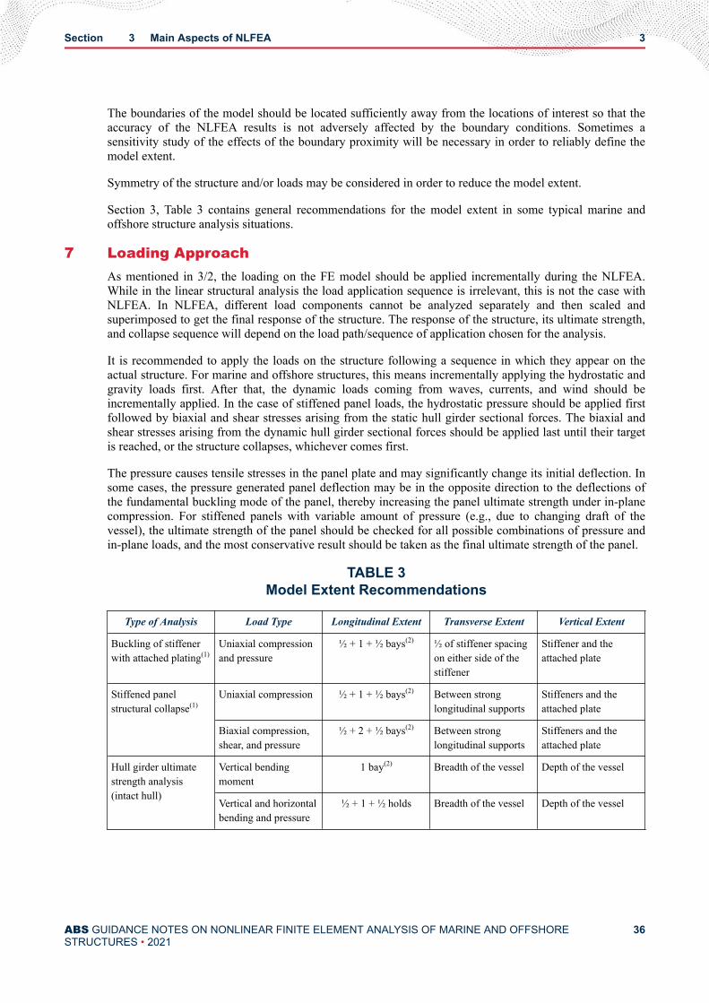
The boundaries of the model should be located sufficiently away from the locations of interest so that theaccuracy of the NLFEA results is not adversely affected by the boundary conditions. Sometimes asensitivity study of the effects of the boundary proximity will be necessary in order to reliably define themodel extent.

Symmetry of the structure and/or loads may be considered in order to reduce the model extent.

Section 3, Table 3 contains general recommendations for the model extent in some typical marine andoffshore structure analysis situations.

7 Loading ApproachAs mentioned in 3/2, the loading on the FE model should be applied incrementally during the NLFEA.While in the linear structural analysis the load application sequence is irrelevant, this is not the case withNLFEA. In NLFEA, different load components cannot be analyzed separately and then scaled andsuperimposed to get the final response of the structure. The response of the structure, its ultimate strength,and collapse sequence will depend on the load path/sequence of application chosen for the analysis.

It is recommended to apply the loads on the structure following a sequence in which they appear on theactual structure. For marine and offshore structures, this means incrementally applying the hydrostatic andgravity loads first. After that, the dynamic loads coming from waves, currents, and wind should beincrementally applied. In the case of stiffened panel loads, the hydrostatic pressure should be applied firstfollowed by biaxial and shear stresses arising from the static hull girder sectional forces. The biaxial andshear stresses arising from the dynamic hull girder sectional forces should be applied last until their targetis reached, or the structure collapses, whichever comes first.

The pressure causes tensile stresses in the panel plate and may significantly change its initial deflection. Insome cases, the pressure generated panel deflection may be in the opposite direction to the deflections ofthe fundamental buckling mode of the panel, thereby increasing the panel ultimate strength under in-planecompression. For stiffened panels with variable amount of pressure (e.g., due to changing draft of thevessel), the ultimate strength of the panel should be checked for all possible combinations of pressure andin-plane loads, and the most conservative result should be taken as the final ultimate strength of the panel.

TABLE 3Model Extent Recommendations

Type of Analysis Load Type Longitudinal Extent Transverse Extent Vertical Extent

Buckling of stiffenerwith attached plating(1)

Uniaxial compressionand pressure

½ + 1 + ½ bays(2) ½ of stiffener spacingon either side of thestiffener

Stiffener and theattached plate

Stiffened panelstructural collapse(1)

Uniaxial compression ½ + 1 + ½ bays(2) Between stronglongitudinal supports

Stiffeners and theattached plate

Biaxial compression,shear, and pressure

½ + 2 + ½ bays(2) Between stronglongitudinal supports

Stiffeners and theattached plate

Hull girder ultimatestrength analysis(intact hull)

Vertical bendingmoment

1 bay(2) Breadth of the vessel Depth of the vessel

Vertical and horizontalbending and pressure

½ + 1 + ½ holds Breadth of the vessel Depth of the vessel



36

Type of Analysis Load Type Longitudinal Extent Transverse Extent Vertical Extent

Hull girder residualstrength analysis(damaged hull)

Vertical bendingmoment

The extent of damage,but no less than½ + 1 + ½ holds

Breadth of the vessel Depth of the vessel

Vertical and horizontalbending and pressure

The extent of damage,but no less than½ + 1 + ½ holds

Breadth of the vessel Depth of the vessel

Impact with ice Line loads and patchload (ABS GuidanceNotes on Ice Class)

Sufficiently beyondthe length of theapplied ice patch

load(3)

From side shell tocenterline

Between deck abovestructural region ofinterest and turn ofbilge

Ship-to-ship collision Impact with bulbousbow of striking ship

1 hold From side shell tocenterline

Depth of the vessel

Notes:

1 For stiffeners and stiffened panels, the longitudinal direction coincides with the direction of the stiffeners, and thevertical direction is perpendicular to the plating.

2 Bay is the area between adjacent transverse frames.

3 For ice class vessels, the model longitudinal extent needs to be sufficient such that the boundary conditions do notsignificantly influence the results of the NLFEA.

Some structures may undergo large deflections. As a result, the load direction and/or magnitude maychange. This should be carefully considered during the analysis.

When performing NLFEA, there are two main types of incremental loading approach:

● Displacement control

● Load control

7.1 Displacement ControlThis loading approach consists of incrementing the displacements of the structure’s boundary. In case ofthe hull girder under bending moments, rigid body rotation of the model end cross sections (curvature) isincremented.

Displacement control is primarily used because it is easy to trace the behavior of the structure in the post-collapse region beyond the limit point (point A in Section 3, Figure 2). However, it requires special postprocessing of the stress results in order to find the forces and moments at various cross sections of interestinside the structure. Another issue of pre-imposing a curvature on the FE model is that the real-worldbehavior of marine and offshore structures is not controlled by displacements, but by loads (forces andmoments), and the input of the displacement may not accurately represent the failure process as describedin [8].

Care should be taken when displacement control is applied to asymmetric structures (e.g., asymmetricallydamaged hull girder). In this case, incrementing the rotation of the end cross sections around the horizontalaxis will result in the development of the horizontal bending moment in addition to the intended verticalbending moment, if the neutral axis of the model is not allowed to rotate. However, if boundary conditionsapplied at the ends of a sufficiently long FE model of the hull (e.g., ½ + 1 + ½ holds – see Section 3, Table3) prevent the development of internal axial forces, then the neutral axis of the hull away from the endswill be allowed to shift and rotate.



37

7.2 Load ControlThis loading approach consists of incrementing the loads (force, moment, pressure). The major drawbackof this approach is that it is not possible, in general, to obtain the negative slope portion of the load-displacement curve when using the N-R iteration algorithm in a static analysis. This creates uncertainty onthe calculated ultimate strength value (i.e., the confidence that the ultimate capacity of a structure has beenreached without being able to identify the highest peak in the load-displacement curve). This is especiallyimportant if the load-displacement curve of the structure has more than one peak. The loss of convergenceduring static analysis will, of course, occur just as the first peak is being reached. Therefore, unless the firstpeak is also the highest, it will usually be impossible to find the ultimate strength of the structure usingload control during a static analysis with N-R algorithms.

The Arc-Length algorithm (see 3/3.2) can trace the static solution into the post ultimate strength region. Inpractice, however, for complex marine and offshore structures, the Arc-Length algorithm may fail toconverge as soon as local instabilities start to occur. If the static analysis using Arc-Length algorithm failsto converge beyond the first peak of the load-displacement curve, then the quasi-static analysis (see 3/5.3)may offer a solution. However, it may be quite difficult to control the kinetic energy of the system beyondthe first peak of the load-displacement curve, as mentioned in 3/5.3.

8 Boundary ConditionsEvery NLFEA will require some level of assumptions regarding the boundary conditions. The importanceof realistically representing the boundary conditions in the finite element model is even more important fornonlinear analyses than for linear analyses. When assumptions regarding the boundary conditions need tobe made, they should be made in such a way as to lead to a conservative response of the structure.

Using assumptions that are valid for small displacement linear analysis for NLFEA should be donecautiously. For example, the assumption that the hull girder cross sections remain plane is valid inside thesimple beam theory but ceases to hold when shear and torsion effects are included as part of theTimoshenko beam theory. However, this assumption is considered adequate in many linear analyses,especially for vessels with closed cross-sections. In a nonlinear analysis, it becomes less accurate,especially as certain parts of the structure begin to yield or buckle. The assumption can still be made inNLFEA, but only when the locations of interest are sufficiently away from the end cross sections.

The examples of typical boundary conditions for the analysis of stiffened panels, hull girders, andcontainer stacks are given in Appendix 1. Boundary conditions for the analysis of side structure of a vesselsubject to ice loads are given in the ABS Guidance Notes on Ice Class.

9 Material ModelMild and high tensile strength steels used for building marine and offshore structures are elasto-plasticmaterials. They are characterized by an elastic region up to the yield point and an elasto-plastic regionconsisting of a yield plateau and a strain hardening region where the material yield point increases whenthe structure is unloaded and subsequently reloaded, as shown in Section 3, Figure 4. When the initial yieldstress, σY, is exceeded, plastic strains (deformations) start to develop in the structure. In the case ofunloading at point A, the stress response follows a straight line to point B with the same elastic modulus,E. The elastic strain, εel, is recovered at point B, but the plastic strain, εp, remains. When the structure isloaded again (point B to point A), the stress response follows the same path as on unloading. However, thistime the material will start to yield at σY1 ≥ σY. Therefore, the material hardens due to the plastic strains.

The material model used in the NLFEA should be able to adequately describe the material behavior duringmonotonic loading, unloading, reversed loading, and repeated cyclic loading if needed as in the low-cyclefatigue analyses.

The commonly used J2 metal plasticity theory [9] provides high-fidelity models for elasto-plastic materialssuch as mild and high tensile steels used in the marine and offshore industries and consists of the followingthree main elements:



38

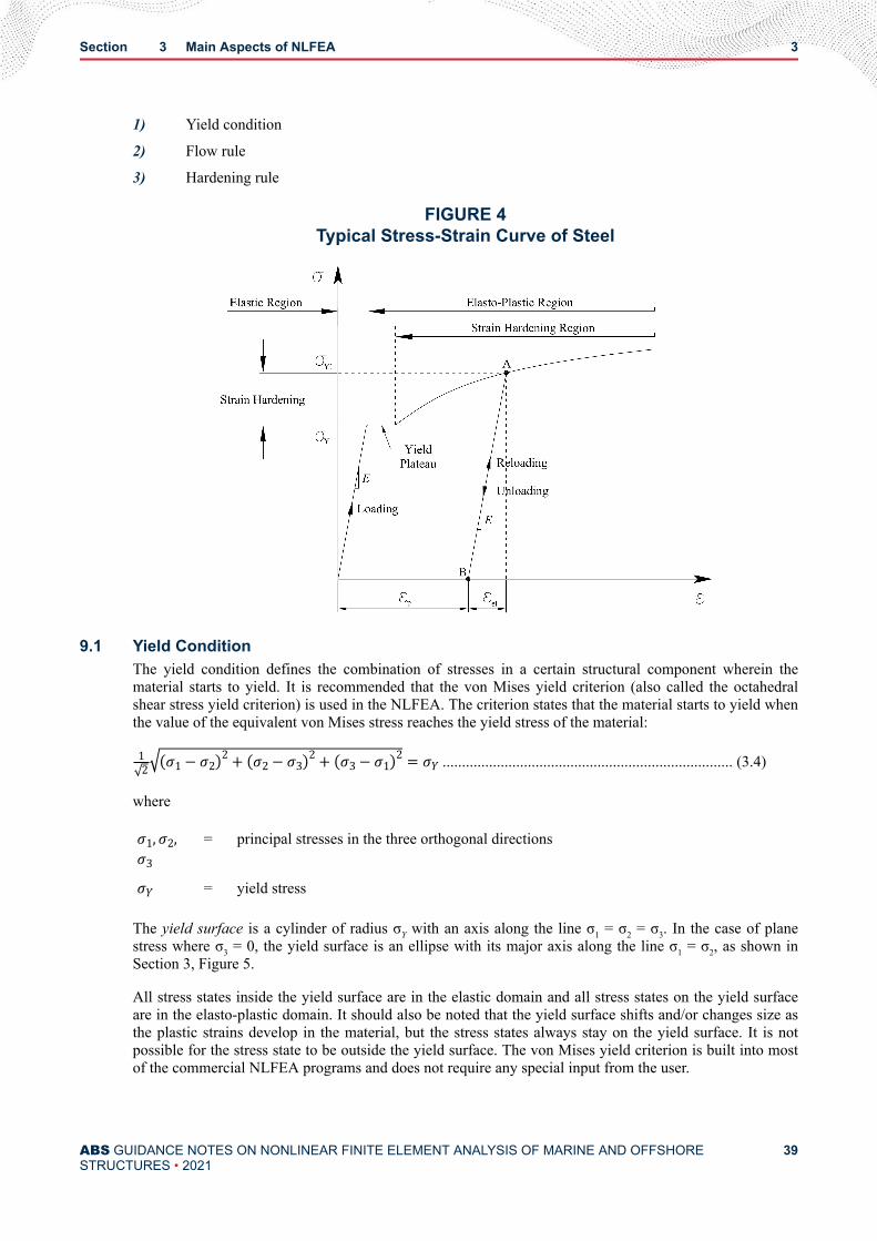
1) Yield condition

2) Flow rule

3) Hardening rule

FIGURE 4Typical Stress-Strain Curve of Steel

9.1 Yield ConditionThe yield condition defines the combination of stresses in a certain structural component wherein thematerial starts to yield. It is recommended that the von Mises yield criterion (also called the octahedralshear stress yield criterion) is used in the NLFEA. The criterion states that the material starts to yield whenthe value of the equivalent von Mises stress reaches the yield stress of the material:12 σ1− σ2 2+ σ2− σ3 2+ σ3− σ1 2 = σY ........................................................................... (3.4)

whereσ1,σ2,σ3 = principal stresses in the three orthogonal directions

σY = yield stress

The yield surface is a cylinder of radius σY with an axis along the line σ1 = σ2 = σ3. In the case of planestress where σ3 = 0, the yield surface is an ellipse with its major axis along the line σ1 = σ2, as shown inSection 3, Figure 5.

All stress states inside the yield surface are in the elastic domain and all stress states on the yield surfaceare in the elasto-plastic domain. It should also be noted that the yield surface shifts and/or changes size asthe plastic strains develop in the material, but the stress states always stay on the yield surface. It is notpossible for the stress state to be outside the yield surface. The von Mises yield criterion is built into mostof the commercial NLFEA programs and does not require any special input from the user.



39

FIGURE 5Von Mises Yield Surface for Plain Stress

9.2 Flow RuleThe flow rule describes the relationship between the plastic strain increment and the stress increment oncethe stress state is on the yield surface. In other words, it describes how the plastic straining develops(flows). The plastic strain increment direction is usually assumed to be normal to the yield surface (see3/9.1). Due to this association between the plastic strain increment direction and the yield surface normal,the rule is called the associated flow rule and is used in most commercial NLFEA programs by default.

According to the plasticity theory, the relationship between the plastic strain increments and stressincrements (the flow rule) can be described by a single uniaxial stress-plastic strain curve for all possiblestress states. This stress-strain curve is called the flow curve and is usually the only input required from theuser to define the flow rule. The uniaxial tension test data, if available, should be used. If this is not thecase, the design stress-strain curves for mild and high tensile steels from 3/9.4 may be used instead.

9.3 Hardening RuleThe hardening rule describes how the yield surface evolves when plastic straining occurs. Three basichardening models are usually used and are available in most commercial NLFEA programs:

1) Kinematic hardening

2) Isotropic hardening

3) Combined kinematic and isotropic hardening

9.3.1 Kinematic HardeningThe kinematic hardening model assumes that the yield surface does not change in size or shape,but simply shifts in the stress space by a tensor, α, called backstress. The shifting of the yieldsurface in one direction causes the asymmetry of yield stress in tension and subsequentcompression of the material. For example, the material subjected to tension will yield at σY. If theloading is then reversed and compression force is applied, the material will yield at a value that issmaller, in absolute terms, compared to σY (see Section 3, Figure 6 for a case of uniaxial stress).This earlier yielding on load reversal is called the Bauschinger effect and is observed in mostengineering metals. Therefore, the chosen hardening model for marine and offshore steels shouldcontain the kinematic hardening component if reversed loading is applied during the analysis.



40

A simplified version of the general (nonlinear) kinematic hardening model is the linear kinematichardening model where stresses after yielding depend linearly on plastic strains. Therefore, thelinear kinematic hardening model should only be used if the bilinear stress-strain curve is anadequate representation of the material, which is seldom the case.

9.3.2 Isotropic HardeningThe isotropic hardening model assumes that the yield surface expands equally in all directionswhen plastic straining occurs. In this case, the material in subsequent compression starts to yield atthe new yield stress, σY1, which is greater in absolute terms than the initial yield stress of thematerial, σY (see Section 3, Figure 7). Therefore, the isotropic hardening model predicts theopposite of the Bauschinger effect. The isotropic hardening model should only be used on its ownif reversed loading is not applied during the analysis (e.g., ultimate strength analysis of a hull-girder or a local structure).

FIGURE 6Kinematic Hardening Model

FIGURE 7Isotropic Hardening Model



41

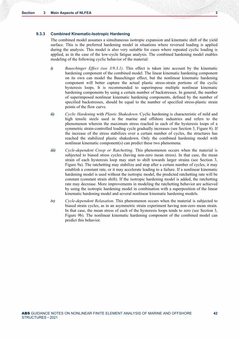
9.3.3 Combined Kinematic-Isotropic HardeningThe combined model assumes a simultaneous isotropic expansion and kinematic shift of the yieldsurface. This is the preferred hardening model in situations where reversed loading is appliedduring the analysis. This model is also very suitable for cases where repeated cyclic loading isapplied, as in the case of the low-cycle fatigue analysis. The combined hardening model enablesmodeling of the following cyclic behavior of the material:

i) Bauschinger Effect (see 3/9.3.1). This effect is taken into account by the kinematichardening component of the combined model. The linear kinematic hardening componenton its own can model the Bauschinger effect, but the nonlinear kinematic hardeningcomponent will better capture the actual plastic stress-strain portions of the cyclichysteresis loops. It is recommended to superimpose multiple nonlinear kinematichardening components by using a certain number of backstresses. In general, the numberof superimposed nonlinear kinematic hardening components, defined by the number ofspecified backstresses, should be equal to the number of specified stress-plastic strainpoints of the flow curve.

ii) Cyclic Hardening with Plastic Shakedown. Cyclic hardening is characteristic of mild andhigh tensile steels used in the marine and offshore industries and refers to thephenomenon wherein the maximum stress reached in each of the hysteresis loops of asymmetric strain-controlled loading cycle gradually increases (see Section 3, Figure 8). Ifthe increase of the stress stabilizes over a certain number of cycles, the structures hasreached the stabilized plastic shakedown. Only the combined hardening model withnonlinear kinematic component(s) can predict these two phenomena.

iii) Cycle-dependent Creep or Ratchetting. This phenomenon occurs when the material issubjected to biased stress cycles (having non-zero mean stress). In that case, the meanstrain of each hysteresis loop may start to shift towards larger strains (see Section 3,Figure 9a). The ratchetting may stabilize and stop after a certain number of cycles, it mayestablish a constant rate, or it may accelerate leading to a failure. If a nonlinear kinematichardening model is used without the isotropic model, the predicted ratchetting rate will beconstant (constant strain shift). If the isotropic hardening model is added, the ratchettingrate may decrease. More improvements in modeling the ratchetting behavior are achievedby using the isotropic hardening model in combination with a superposition of the linearkinematic hardening model and several nonlinear kinematic hardening models.

iv) Cycle-dependent Relaxation. This phenomenon occurs when the material is subjected tobiased strain cycles, as in an asymmetric strain experiment having non-zero mean strain.In that case, the mean stress of each of the hysteresis loops tends to zero (see Section 3,Figure 9b). The nonlinear kinematic hardening component of the combined model canpredict this behavior.



42

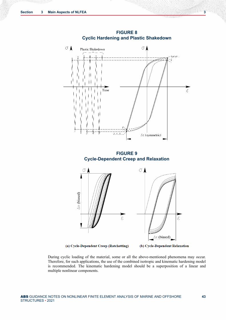
FIGURE 8Cyclic Hardening and Plastic Shakedown

FIGURE 9Cycle-Dependent Creep and Relaxation

During cyclic loading of the material, some or all the above-mentioned phenomena may occur.Therefore, for such applications, the use of the combined isotropic and kinematic hardening modelis recommended. The kinematic hardening model should be a superposition of a linear andmultiple nonlinear components.



43

Different commercial NLFEA packages may have different implementations of various hardeningmodels. The determination of parameters of such models is outside the scope of these GuidanceNotes. Some general guidelines are provided below. Usually, the NLFEA program documentationwill contain details on how to calibrate the parameters of hardening models based on test data.

The parameters of the isotropic hardening model may be calibrated directly from the strain-controlled cyclic test data for the material in question. Because the isotropic hardening model doesnot predict different hardening behavior at different strain ranges, attention should be given toperforming the calibration test at a constant strain range corresponding to the strain range expectedduring the analysis.

The parameters of the kinematic hardening model may be calibrated based on the stress-plasticstrain data from a monotonic uniaxial tension test. In this way, the kinematic hardening parametersare essentially calibrated based on the first half-cycle and will only be relevant if the analysisconsists of only a few cycles.

For analyses consisting of many cycles, especially where a stabilized response is of interest, theparameters of the kinematic hardening model should be calibrated based on the stabilized stress-plastic strain hysteresis loop curve from a symmetric strain-controlled cyclic test. Somecommercial NLFEA programs will perform the calibration automatically based on the suppliedtest data.

Cyclic stress-plastic strain curves for a particular material may be used as an approximation of thestabilized stress-plastic strain hysteresis loop curve, but it needs to be expanded by a scale factorof two [3]. Care should also be taken to supply the test data in the format that is required by theNLFEA program.

9.4 Stress-Strain Curves (Flow Curves)When reversed loading or cyclic loading does not have to be modeled, usually the only material parametersthat need to be supplied are the elastic parameters (Poisson ratio, v, elastic modulus, E, and yield stress,σY), mass density, ρ, and the uniaxial stress-strain curve describing the nonlinear plastic flow (flow curve).Ideally, the material parameters should be obtained from tests of the selected material. In the case when theuniaxial test data sets are not available for the materials used in the NLFEA, the data presented in thisSubsection may be used as characteristic design material properties.

The stress-strain pairs from the uniaxial tension tests are usually given in terms of engineering stresses andstrains, where both physical quantities are calculated based on the initial cross section and length of a testspecimen, respectively. On the other hand, most commercial NLFEA require the definition of the flowcurve in terms of the true stresses and strains, which are calculated based on the specimen’s instantaneouscross-section and instantaneous strain increments, respectively. The relationships between true andengineering stresses and strains are given as:σ = σeng εeng+ 1 ............................................................................................................................. (3.5)ε = ln εeng+ 1 ................................................................................................................................. (3.6)

whereσ = true stressε = true strainσeng = engineering stressεeng = engineering strain



44

Eq. 3.5 and 3.6 are only valid up to the onset of necking, when the ultimate tensile stress is reached. Afternecking, the true stresses and strains may be obtained using precise measurements of the instantaneouscross-sectional area of the specimen:σ = FS . . . . . . . . . . . . . . . . . . . . . . . . . . . . . . . . . . . . . . . . . . . . . . . . . . . . . . . . . . . . . . . . . . . . . (3 . 7)ε = ln S0S . . . . . . . . . . . . . . . . . . . . . . . . . . . . . . . . . . . . . . . . . . . . . . . . . . . . . . . . . . . . . . . . (3 . 8)whereF = instantaneous axial tensionS = current cross-sectional area of the test specimenS0 = initial cross-sectional area of the test specimen

In addition to the true flow curves, commercial NLFEA programs usually require that the true stresses bedefined versus the plastic portion, εp, of the total true strain ε. True plastic strains can be calculated bysubtracting the elastic strains from the total true strains as follows:εP = ε− εel = ε − σE . . . . . . . . . . . . . . . . . . . . . . . . . . . . . . . . . . . . . . . . . . . . . . . . . . . . . . . (3 . 9)whereεel = σE = elastic portion of the true strain (see also Section 3, Figure 4).

The engineering stress-strain curves for most steels used in marine and offshore structures exhibit asoftening region after the ultimate stress point is reached. This region is characterized by the negative slopeof the flow curve and occurs due to necking (localized deformation of the specimen’s cross section duringuniaxial tests). The true stress-strain curves for most steels used in marine and offshore structures willusually not have the softening region as shown in Section 3, Figure 10.

FIGURE 10True vs. Engineering Flow Curves



45

The proposed model for the true flow curves is based on calibration analysis on over 500 engineeringstress-strain data sets for structural carbon steels with the yield stress ranging from 235 N/mm2 (23.96kgf/mm2, 34084 psi) to 960 N/mm2 (97.89 kgf/mm2, 139236 psi), as specified in [10]. The model is acombination of a bi-linear and a nonlinear strain hardening model. The model only requires the knowledgeof the elastic modulus, E, the engineering yield stress, σY,eng, and the engineering ultimate stress, σU,eng. Allthree parameters are usually readily available to the engineer for any steel grade.

The true flow curve is given as follows:

σ ε =

E eε− 1 eε if ε ≤ ln εy, eng+ 1σY, engeε if ln εy, eng+ 1 < ε ≤ ln εsℎ, eng+ 1σY, eng+ σU, eng− σY, eng 1− 24015 eε − 1 − εsℎ, engεu, eng − εsℎ, eng if ln εsℎ, eng+ 1 < ε ≤ ln εu, eng+ 1+ 2 eε − 1 − εsℎ, engεu, eng − εsℎ, eng

1 + 400 eε − 1 − εsℎ, engεu, eng − εsℎ, eng 5 1/5 eεKεn if ε > ln εu, eng+ 1

(3 . 10)

whereεy, eng = σY, engE . . . . . . . . . . . . . . . . . . . . . . . . . . . . . . . . . . . . . . . . . . . . . . . . . . . . . . . (3 . 11)εsℎ, eng = 0.1 σY, engσU, eng – 0.055 , but 0.015 ≤ εsℎ, eng ≤ 0.03 . . . . . . . . . . . . . . . . . . . . . (3 . 12)εu, eng = 0.6 1− σY, engσU, eng , but εu, eng ≥ 0.06 . . . . . . . . . . . . . . . . . . . . . . . . . . . . . . (3 . 13)K = σU, eng en n . . . . . . . . . . . . . . . . . . . . . . . . . . . . . . . . . . . . . . . . . . . . . . . . . . . . . . . (3 . 14)n = ln εu, eng+ 1 . . . . . . . . . . . . . . . . . . . . . . . . . . . . . . . . . . . . . . . . . . . . . . . . . . . . . (3 . 15)The material model is schematically explained in Section 3, Figure 11, where the axes are the true stressand true strain. It should be noted that:εy, eng = engineering strain at the onset of yieldingεsℎ, eng = engineering strain at the start of the strain hardening regionεu, eng = engineering strain at the point where ultimate engineering stress σu, eng, is reached (the

onset of necking)

The material model parameters for common steel grades used in the marine and offshore industries areshown in Section 3, Table 4.

The recommended design true flow curve plots for common marine and offshore steels are shown inSection 3, Figure 12.

Appendix 2 contains design true flow curves for common steel grades used in the marine and offshoreindustries. Both total true strains and plastic true strains are given in the tables.



46

9.5 Strain-Rate EffectsThe effect of strain rate on the mechanical properties of the material are often neglected during the NLFEAof marine and offshore structures. However, in cases of high-speed collision or impact analyses, theseeffects may become important.

In general, material flow curves harden, and the fracture strain decreases as the strain rate increases. Strain-rate hardening should be modeled using the Cowper-Symonds equation to stretch the true flow curve alongthe y-axis by a constant factor that depends on the strain rate, ε:σ ε dyn = σ ε 1 + εC 1/q . . . . . . . . . . . . . . . . . . . . . . . . . . . . . . . . . . . . . . . . . . . . . . . . . (3 . 16)whereσ ε dyn = dynamic true flow curveσ(ε) = static true flow curveC, q = parameters of the Cowper-Symonds model

C and q should be calibrated based on the experimental data. In the absence of more relevant experimentaldata, the parameter values from Section 3, Table 5 may be used when the plastic strains during the analysisare small.

FIGURE 11Schematic Description of the Recommended Material Model



47

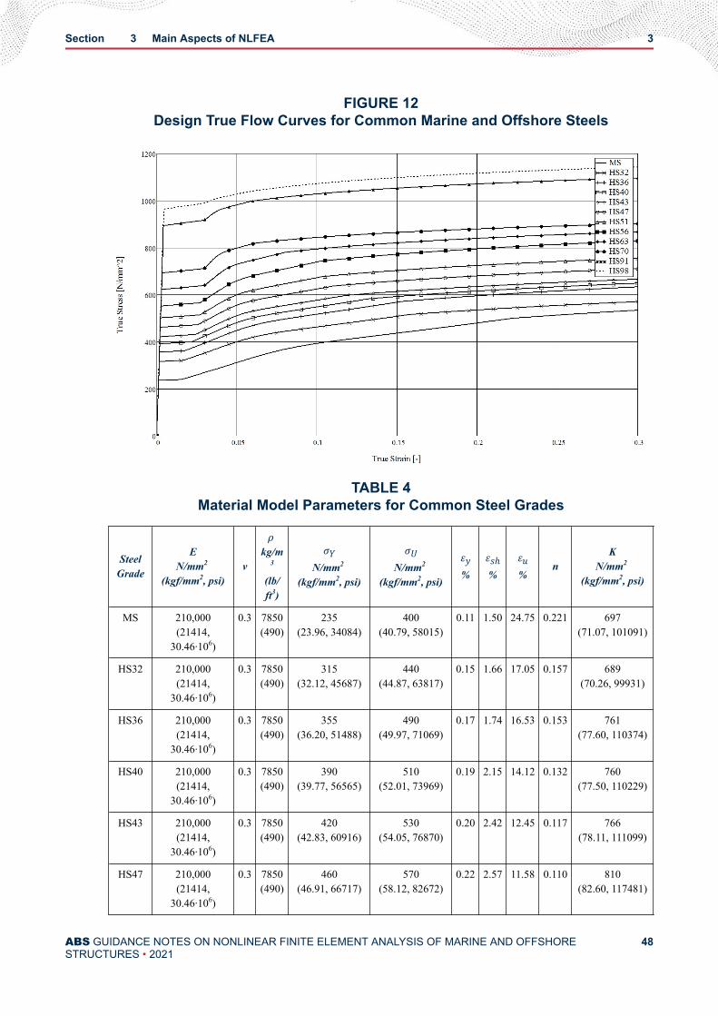
FIGURE 12Design True Flow Curves for Common Marine and Offshore Steels

TABLE 4Material Model Parameters for Common Steel Grades

SteelGrade

EN/mm2

(kgf/mm2, psi)ν

ρ kg/m

3

(lb/ft3)

σYN/mm2

(kgf/mm2, psi)

σUN/mm2

(kgf/mm2, psi)

εy%

εsℎ%

εu%

nK

N/mm2 (kgf/mm2, psi)

MS 210,000(21414,

30.46∙106)

0.3 7850(490)

235(23.96, 34084)

400(40.79, 58015)

0.11 1.50 24.75 0.221 697(71.07, 101091)

HS32 210,000(21414,

30.46∙106)

0.3 7850(490)

315(32.12, 45687)

440(44.87, 63817)

0.15 1.66 17.05 0.157 689(70.26, 99931)

HS36 210,000(21414,

30.46∙106)

0.3 7850(490)

355(36.20, 51488)

490(49.97, 71069)

0.17 1.74 16.53 0.153 761(77.60, 110374)

HS40 210,000(21414,

30.46∙106)

0.3 7850(490)

390(39.77, 56565)

510(52.01, 73969)

0.19 2.15 14.12 0.132 760(77.50, 110229)

HS43 210,000(21414,

30.46∙106)

0.3 7850(490)

420(42.83, 60916)

530(54.05, 76870)

0.20 2.42 12.45 0.117 766(78.11, 111099)

HS47 210,000(21414,

30.46∙106)

0.3 7850(490)

460(46.91, 66717)

570(58.12, 82672)

0.22 2.57 11.58 0.110 810(82.60, 117481)



48

SteelGrade

EN/mm2

(kgf/mm2, psi)ν

ρ kg/m

3

(lb/ft3)

σYN/mm2

(kgf/mm2, psi)

σUN/mm2

(kgf/mm2, psi)

εy%

εsℎ%

εu%

nK

N/mm2 (kgf/mm2, psi)

HS51 210,000(21414,

30.46∙106)

0.3 7850(490)

500(50.99, 72519)

610(62.20, 88473)

0.24 2.70 10.82 0.103 854(87.08, 123862)

HS56 210,000(21414,

30.46∙106)

0.3 7850(490)

550(56.08, 79771)

670(68.32, 97175)

0.26 2.71 10.75 0.102 937(95.55, 135900)

HS63 210,000(21414,

30.46∙106)

0.3 7850(490)

620(63.22, 89923)

720(73.42, 104427)

0.30 3.00 8.33 0.080 955(97.38, 138511)

HS70 210,000(21414,

30.46∙106)

0.3 7850(490)

690(70.36, 100076)

770(78.52, 111679)

0.33 3.00 6.23 0.061 969(98.81, 140542)

HS91 210,000(21414,

30.46∙106)

0.3 7850(490)

890(90.75, 129084)

940(95.85, 136335)

0.42 3.00 6.00 0.058 1176(119.92,170564)

HS98 210,000(21414,

30.46∙106)

0.3 7850(490)

960(97.89, 139236)

980(99.93, 142137)

0.46 3.00 6.00 0.058 1226(125.02,177816)

TABLE 5Cowper-Symonds Parameters for Small Plastic Strains

Cowper-Symonds Parameters

C [s-1] q [-]

Mild Steels 40.4 5

High Tensile Steels 3200 5

Since parameters C and q may depend on the plastic strains and the plate thickness as shown in [11],especially for mild steels, it is necessary to use the parameters that are calibrated at the plastic strain leveland the plate thickness relevant for the problem to be analyzed by the NLFEA. If the expected strainsduring the NLFEA are very large, the parameter values from Section 3, Table 5 for mild steel may lead tooverestimation of the hardening effect for larger plastic strains. In the absence of more accurate values, thestrain rate may be estimated using the following expression:ε = V02δ . . . . . . . . . . . . . . . . . . . . . . . . . . . . . . . . . . . . . . . . . . . . . . . . . . . . . . . . . . . . . . . . . (3 . 17)whereV0 = initial speed of the dynamic loadδ = average displacement of the structural element

For ship collisions, the estimated strain rate is in the range of 0.5 s-1 to 5 s-1, as stated in [12].



49

10 Geometric ImperfectionsDuring the fabrication of thin-walled marine and offshore structures (metal cutting, rolling, forming,welding, and heat treatment), some geometric imperfections (nonuniformities in shape, eccentricities, andlocal imperfections) and residual stresses are inevitably introduced and can affect their structural behavior,especially the ultimate strength. Accidental limit states due to collision, grounding, impact with ice, orexplosion are not likely to be affected by the initial imperfections and residual stresses in the structure.However, the initial imperfections may help avoid the numerical instabilities during the solution process,regardless of the type of limit state that is being analyzed.

The shape and size of initial geometric imperfections may have a significant impact on the ultimate limitstate of the structure and its collapse mechanism, especially for structures that are sensitive to the initialimperfections. Therefore, a sound understanding of the effect of imperfection patterns and magnitudes onthe analyzed or similar structures may be necessary. The geometric imperfections can be treated using thefollowing four different approaches:

1) Impose the measured initial imperfection pattern onto the FE model

2) Linear superposition of buckling eigenmodes from the eigenvalue buckling analysis

3) Direct shape definition through the specification of nodal coordinates

4) Using the deformation shape from a linear static analysis

The following Paragraphs contain recommended practices related to each of the above-mentionedtreatments of the geometric imperfections. The imperfection magnitudes given in 3/10.3 can be used inapproaches 2, 3, and 4 from the above list and are applicable to the basic building blocks of marine andoffshore structures – stiffened panels. Imperfections obtained in this way can be considered as equivalentimperfections that represent the combined effects of the initial imperfections and the residual stresses.Other equivalent imperfection magnitudes may be considered, depending on fabrication tolerances andpost weld heat treatment. The choice of equivalent imperfection magnitudes should be documented.

10.1 Imposing Measured ImperfectionsThis is the most accurate approach to treating the geometric imperfections. However, measurement ofrandom imperfection patterns on real marine and offshore structures is complex and time consuming, andthe measured imperfections are usually not available. The measured imperfections, as opposed to theequivalent imperfections, do not account for the effects of residual stresses.

10.2 Linear Superposition of EigenmodesThis is usually the most convenient method and is recommended for large and complex structures such as asection or the entire hull girder of a vessel. A linear eigenvalue buckling analysis should be performedfirst. Then, only four eigenmodes should be linearly combined and scaled to obtain the imperfectionpattern with the desired amplitudes. The following four buckling modes should be selected:

1) Global buckling mode that best describes the overall buckling of the stiffened panel (plate andstiffeners) between the strong supporting members

2) Local buckling mode that best describes the local buckling of the plate between the stiffeners

3) Local buckling mode that best describes the local buckling of the stiffener web plates

4) Local buckling mode that best describes the local sideways tripping of the stiffeners

More information regarding the recommended geometry of the global and local imperfection patterns aswell as their recommended equivalent magnitudes is given in 3/10.3.

Attention should be paid to imposing the relevant boundary conditions during the eigenvalue bucklinganalysis so that realistic buckling modes can be obtained.



50

Initial imperfections are usually imposed over the parts of the structure that are susceptible to bucklingunder compressive loads. In case of the hull girder, imperfections should be applied across the top hullgirder flange (deck) when the hull is in sagging, or across the bottom flange (double bottom) when the hullis in hogging. In the longitudinal direction, the imperfections should be specified across three adjacent webframe spacings at the weakest sections of the hull where failure is expected.

This method usually produces the most conservative imperfection pattern because the main plate andstiffener buckling modes will be triggered during the analysis.

10.3 Direct Shape DefinitionDirect shape definition uses regular imperfection patterns based on trigonometric functions to describe theinitial imperfections by manually offsetting all the nodes in the structure. Attention should be paid toachieving consistency between nodal offsets of separately treated regions of the marine or the offshorestructure.

Imperfection patterns based on regular trigonometric functions, and similar to the global and local bucklingmodes listed in 3/10.2, should be selected for stiffened panels (see Section 3, Figure 13).

10.3.1 Global Imperfections of the Stiffened PanelThe global imperfections of the panel are given as vertical displacements in the z-axis direction ofall the panel nodes depending only on the original in-plane (x and y) coordinates of the stiffenedpanel nodes (see Section 3, Figure 13). The vertical displacements may be calculated as:σz, panel = a750cosπxa sinπyB . . . . . . . . . . . . . . . . . . . . . . . . . . . . . . . . . . . . . . . . . . . . (3 . 18)wherea = distance between the strong stiffened panel supports in the x direction (e.g., between

web frames)B = total breadth of the stiffened panel in the y direction (see Section 3, Figure 13)

Eq. 3.18 creates one half-wave between the strong supports in the x direction and one half-wavebetween the strong supports in the y direction, as shown in Section 3, Figure 14. Therecommended maximum out-of-plane global deformation of the stiffeners with the attachedplating is a/750.

If the origin of the coordinate system is shifted in the x direction to the strong transverse supportinstead of in between the strong transverse supports, then the cosine function in Eq. 3.18 should bereplaced with the sine function.



51

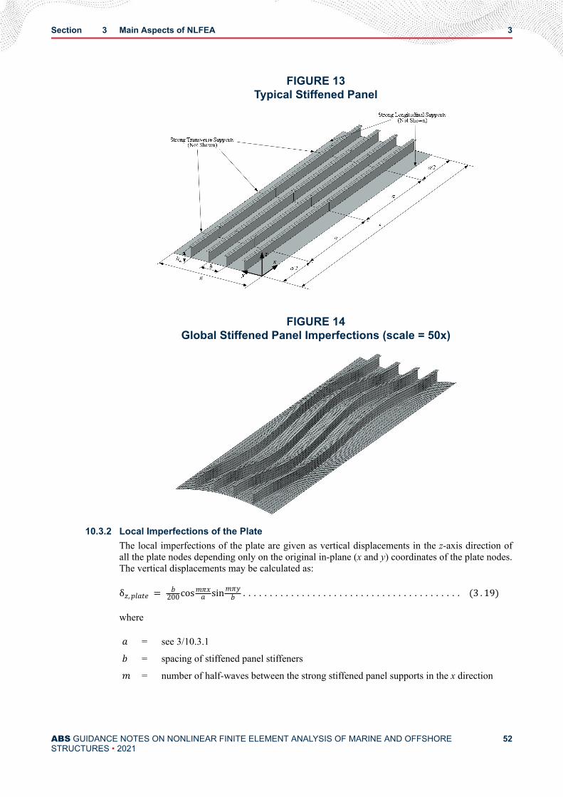
FIGURE 13Typical Stiffened Panel

FIGURE 14Global Stiffened Panel Imperfections (scale = 50x)

10.3.2 Local Imperfections of the PlateThe local imperfections of the plate are given as vertical displacements in the z-axis direction ofall the plate nodes depending only on the original in-plane (x and y) coordinates of the plate nodes.The vertical displacements may be calculated as:δz, plate = b200cosmπxa sinmπyb . . . . . . . . . . . . . . . . . . . . . . . . . . . . . . . . . . . . . . . . . (3 . 19)wherea = see 3/10.3.1b = spacing of stiffened panel stiffenersm = number of half-waves between the strong stiffened panel supports in the x direction



52

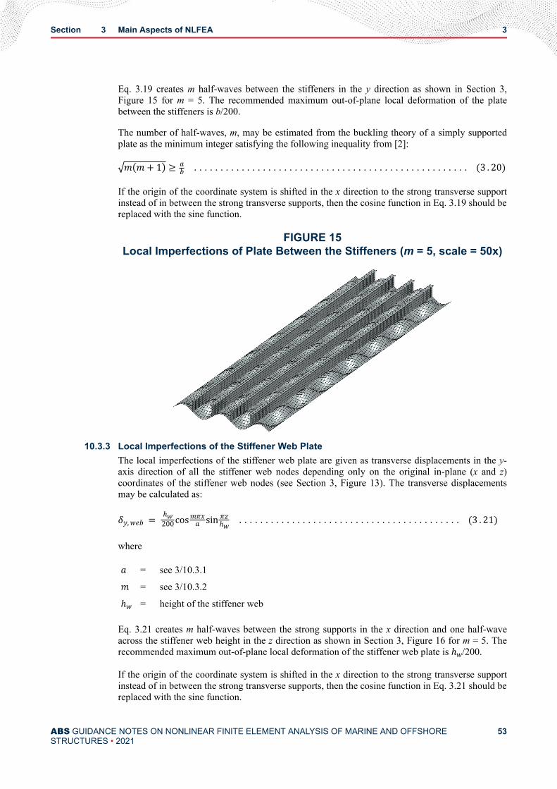
Eq. 3.19 creates m half-waves between the stiffeners in the y direction as shown in Section 3,Figure 15 for m = 5. The recommended maximum out-of-plane local deformation of the platebetween the stiffeners is b/200.

The number of half-waves, m, may be estimated from the buckling theory of a simply supportedplate as the minimum integer satisfying the following inequality from [2]:m m+ 1 ≥ ab . . . . . . . . . . . . . . . . . . . . . . . . . . . . . . . . . . . . . . . . . . . . . . . . . . . . (3 . 20)If the origin of the coordinate system is shifted in the x direction to the strong transverse supportinstead of in between the strong transverse supports, then the cosine function in Eq. 3.19 should bereplaced with the sine function.

FIGURE 15Local Imperfections of Plate Between the Stiffeners (m = 5, scale = 50x)

10.3.3 Local Imperfections of the Stiffener Web PlateThe local imperfections of the stiffener web plate are given as transverse displacements in the y-axis direction of all the stiffener web nodes depending only on the original in-plane (x and z)coordinates of the stiffener web nodes (see Section 3, Figure 13). The transverse displacementsmay be calculated as:δy,web = ℎw200cosmπxa sin πzℎw . . . . . . . . . . . . . . . . . . . . . . . . . . . . . . . . . . . . . . . . . . (3 . 21)wherea = see 3/10.3.1m = see 3/10.3.2ℎw = height of the stiffener web

Eq. 3.21 creates m half-waves between the strong supports in the x direction and one half-waveacross the stiffener web height in the z direction as shown in Section 3, Figure 16 for m = 5. Therecommended maximum out-of-plane local deformation of the stiffener web plate is ℎw/200.




53

FIGURE 16Local Imperfections of Stiffener Webs (m = 5, scale = 50x)

10.3.4 Local Tripping Imperfections of the StiffenerThe local tripping imperfections of the stiffener are given as rotations of the stiffener about thepoint where it is attached to the plate. The transverse and vertical displacements of the stiffenerweb nodes may be calculated as:δy,web = z sinφ .................................................................................................................... (3.22)δz,web = z cosφ – 1 ........................................................................................................ (3.23)

φ = a750ℎwcosπxa sinπ yweb − ns+ 12 bns − 1 b . . . . . . . . . . . . . . . . . . . . . . . . . . . . . . . . . . . . (3 . 24)wherea = see 3/10.3.1b = see 3/10.3.2ℎw = see 3/10.3.3ns = number of stiffeners between strong longitudinal supportsφ = rotation angle of the stiffenerx,yweb,z = original coordinates of the stiffener web nodes with yweb being constant for each of

the stiffeners

The recommended maximum rotation angle of the stiffener is a/(750ℎw) radians.

Similarly, for the stiffener flange nodes:δy, flange = z2+ y − yweb 2 sin α+ φ – sin α ................................................... (3.25)δz, flange = z2+ y − yweb 2 cos α + φ – cos α .................................................. (3.26)



54

α = tan−1y − ywebz .............................................................................................................. (3.27)

y – yweb is the difference between the original y coordinate of the flange node and the y coordinateof the corresponding web. Eq. 3.25, 3.26, and 3.27 couple the stiffener flange rotation with thestiffener web rotation, as shown in Section 3, Figure 17.

FIGURE 17Local Tripping Imperfections of Stiffeners (scale = 50x)


10.3.5 Combined Imperfections of the Stiffened PanelThe combined global and local imperfections are obtained by linear superposition of all theimperfections calculated in 3/10.3.1 to 3/10.3.4. Section 3, Figure 18 shows the combined initialgeometric imperfections of the stiffened panel. Attention should be paid to confirm that themaximum global and local deflections in a certain direction coincide and have the same sign.

FIGURE 18Combined Imperfections of Stiffened Panel (scale = 25x)



55

10.4 Deformed Shape from Linear Static AnalysisThe deformed structure configuration after the linear static analysis step can be scaled and used as theinitial, unstressed configuration for the NLFEA. The scaling should be performed such that the largest out-of-plane deformation of the plate is equal to the sum of global and local amplitudes (i.e., a/750 + b/200)

Using the deformed shape from the linear static analysis to prescribe initial geometric imperfections is onlyapplicable to simple structures that are not sensitive to the imperfection shapes.

11 Ductile Fracture ModelingWhen simulating ship-to-ship collision, grounding, explosions, and other accidental limit states, it may beimportant to consider ductile fracture of the material. Fracture of the material will have an impact on theglobal collapse mechanism of the structure, it will control possible flooding of the compartments, and mostimportantly, it will affect the total energy absorbed by the structure, which determines its crashworthiness.

Predicting fracture in a material is very complex and requires careful calibration and validation againstexperimental data. Many ductile fracture criteria have been developed, some of them specifically for use inmarine and offshore structures [13]. Many of the ductile fracture criteria predict rupture when theequivalent plastic strain in the material, εp , becomes equal to or larger than the critical fracture strain, εcf:εp ≥ εcf .................................................................................................................................... (3.28)εp is a scalar quantity representing material’s accumulated inelastic deformation. It can be expressed usingthe repeated index notation as follows:εp = ∫0t 23 εijp εijpdt .......................................................................................................................... (3.29)

whereεijp = components of the plastic strain rate tensort = time over which the straining has occurredεijp εijp = ε11p 2+ ε12p 2+ ε13p 2+ ε21p 2+ ε22p 2+ ε23p 2+ ε31p 2+ ε32p 2+ ε33p 2Equivalent plastic strain is readily post-processed in most commercial NLFEA programs. According to theplasticity theory, the uniaxial flow curve (σ-ε) can be taken as the equivalent stress-strain (σ − ε) curve, asshown in Section 3, Figure 19. When εp = εcf, ductile fracture is said to have occurred. Some NLFEAdefine the point where εp = εcf, as the initiation of ductile fracture (point A in Section 3, Figure 19),whereas the actual fracture occurs at a larger critical failure strain εcf′ (point B in Section 3, Figure 19).Between the initiation of fracture and the actual fracture, there is progressive ductile fracture evolutionwith degradation of both the yield stress (softening) and the material stiffness. At the actual point offracture, the stiffness of the structure reduces to zero.

The ductile fracture evolution is heavily dependent on the mesh size. NLFEA programs try to minimizethis mesh dependency by defining the ductile fracture evolution in terms of the equivalent plasticdisplacement, up, instead of equivalent plastic strain. up is zero at ductile fracture initiation and increasesto a value upf at fracture. However, it is recommended to, conservatively, neglect the ductile fractureevolution region of the equivalent stress-strain curve by setting:upf = 0 .............................................................................................................................................. (3.30)

where upf is the equivalent plastic displacement at fracture. This is equivalent to assuming that the fracturehas occurred at initiation when εp = εcf, as many ductile fracture criteria do.



56

Critical failure strain, εcf, depends on stress state in the material, strain rate, and mesh size. However, ithas been shown in [14] that εcf in most reliable ductile fracture criteria for collision simulations of marinestructures can be assumed independent of the stress state and the strain rate. A number of commonly usedfracture criteria assume that εcf is a function of the mesh size and plate thickness only:εcf = f L, t ................................................................................................................................... (3.31)

whereL = length of the finite elementt = plate thickness

Ductile fracture criteria with the form as described with Eq. 3.31, where the critical fracture strain isconstant for a certain mesh size and plate thickness, are not usually implemented in commercial NLFEAprograms. However, such criteria can be implemented using commonly available and well-known criteria,where εcf has a constant term, among other terms, and where the ductile damage accumulates linearly. Onesuch criteria is the Johnson-Cook criteria described in [15] that has five parameters d1, d2, d3, d4, and d5, ofwhich only d1 is the constant term. The criteria given by Eq. 3.31 can be implemented using the Johnson-Cook ductile fracture criteria by setting:d1 = f L, t . . . . . . . . . . . . . . . . . . . . . . . . . . . . . . . . . . . . . . . . . . . (3 . 32)d2 = d3 = d4 = d5 = 0The criteria described by Eq. 3.31 also assume there is no ductile fracture evolution and, therefore, requireupf= 0.

FIGURE 19Ductile Fracture Initiation and Evolution



57

References [13] and [12] describe a number of available fracture criteria that can also be considered.However, care should be taken to use properly calibrated parameters for the material and mesh size used inthe NLFEA.

Usually, the NLFEA program will delete an element that has exceeded the ductile fracture criterion in atleast one integration point, by default.

It is generally recommended to conduct the analyses involving fracture using explicit dynamic or explicitquasi-static analyses. Implicit dynamic or implicit quasi static analyses as well as the static analysis requireiteration algorithms that may fail to converge due to the progressive degradation of yield stress andstiffness, especially in cases where ductile fracture evolution is neglected.

12 Contact ModelingModeling contact between two different bodies is necessary in some scenarios, such as ship collisions,grounding, various structural indentations, and multiple container stacks.

When two different bodies come into contact, a contact pressure will develop in the direction perpendicularto the contacting surfaces. The NLFEA solver will determine the amount of contact pressure acting on bothcontact surfaces based on the user-defined pressure-overclosure relationship. Also, if the contactingsurfaces slip relative to each other, frictional forces will develop in the tangential direction. Therefore,contact interface constitutive properties in the normal and tangential direction need to be defined.

12.1 Definition of Contact Interface Constitutive PropertiesFor the analysis of typical marine and offshore structures where contact modeling is needed, it isrecommended to use the hard contact pressure-overclosure relationship where the contact pressure is zerowhen the surfaces are not in contact. When the surfaces are in contact, the pressure is determined based onthe constraint of no penetration of one surface into another. It is recommended to use the penalty method inorder to enforce the hard contact. The penalty method may allow small penetrations. However, thisnumerical softening may help with the convergence issues. Surfaces that come into contact should beallowed to separate once the contact pressure becomes zero.

If modeling friction is needed, isotropic Coulomb friction model is recommended where the friction isproportional to the force acting normal to the contact surfaces. The proportionality factor is the coefficientof friction. For perpendicular ship-to-ship collisions, the friction force will have a very small impact on theanalysis. However, for ship-to-ship collisions at an oblique angle (raking collisions) or for ship groundingsimulations, friction may become an important factor that should be included in the analysis. Thecoefficient of friction should be carefully calibrated and validated against the available experimental data.For ship-to-ship collisions, values between 0.23 and 0.3 are typically used.

12.2 Definition of Contact PairsApart from defining the contact interface constitutive properties in the normal and tangential directions, theuser may also need to define the surfaces, edges, and vertices on one body that may potentially come intocontact with other surfaces, edges, or vertices on the same body or on another body or bodies. This iscalled contact pair definition. Usually surface-to-surface, edge-to-surface, edge-to-edge, and vertex-to-surface types of contact are allowed.

Some commercial NLFEA programs can assign contact pairs automatically, including self-contact. Thisprocedure is recommended as it simplifies the contact modeling considerably, albeit at potentially highercomputational cost.

If the contact pairs are defined manually, then all potential contact pairs should be identified first. Oneentity in the contact pair is defined as “master” and the other one is defined as “slave”. When contact pairsare defined automatically by the NLFEA program, each entity in the contact pair is defined as both master



58

and slave. When defining master and slave surfaces for surface-to-surface contact, the following generalrecommendations should be followed:

i) The larger surface should be selected as the master surface.

ii) If the surfaces are of similar size, the surface of the stiffer body should be selected as the mastersurface.

iii) If the surfaces are of similar size and stiffness, the surface with a coarser mesh should be selectedas the master surface.

12.3 Initial Overclosures and Rough Surface GeometryInitial overclosures (penetrations) may cause convergence issues and should be resolved. Sometimes thetwo or more structural components are in contact at the beginning of the analysis. Even though the surfacesof the bodies that are in contact may be smooth, they will be faceted during meshing and the nodes of onesurface may penetrate the other surface. Small overclosures at the beginning of the analysis can often beresolved automatically by the NLFEA program without causing any initial strain in the structures. Careshould be taken to minimize such initial overclosures as the NLFEA program will exclude the surfaceswith significant initial overclosures from contact pairs.

Rough surface geometry caused by coarse mesh will decrease the accuracy of contact pressure and frictionforce results. It may also cause two surfaces to stick to each other, preventing sliding of the surfaces.Rough surface geometry may be smoothed by refining the mesh in the areas that are expected to come intocontact or by using automated surface smoothing contact algorithms if they are available in the NLFEAprogram.

It should also be recognized that the NLFEA program will take the thickness of the shell elements intoaccount when determining the existence of the contact between two surfaces. Therefore, putting two shellelement reference surfaces into initial contact will result in an overclosure equal to t1/2 + t2/2, where t1 andt2 are the thicknesses of the two shell elements.

12.4 Contact StabilizationConvergence issues related to unwanted rigid body motions can sometimes occur when modeling contact.Some NLFEA programs offer highly automated contact stabilization based on the introduction of artificialviscous damping without significantly affecting the accuracy of the solution. This is similar to thenumerical stabilization technique used for improving the convergence of the N-R iterations as explained in3/4. Contact stabilization should only be used when necessary to stabilize the convergence issues related tocontact, and its energy should stay below 5% of the total internal energy of the system throughout theanalysis.

13 Mesh Quality and SizeMesh size and quality parameters are even more important for NLFEA compared to linear finite elementanalysis (FEA). If the elements undergo significant distortions during the large-displacement nonlinearanalysis, the accuracy and reliability of the solution may be reduced. Therefore, special attention should begiven to element quality, which can often be defined using the following measures:

i) Element Aspect Ratio. Ratio of maximum to minimum element edge length

ii) Skewness Angle. Difference between the right angle and the smallest angle between intersectingelement mid-lines

iii) Warping Angle. Out-of-plane element warping

iv) Corner Angle. Angle between element edges at a corner

v) Jacobian. Measure of the element’s deviation from an ideal shape



59

In order to increase the accuracy and reliability of the NLFEA, the recommended element quality measurelimits for quadrilateral shell and solid brick elements are given in Section 3, Table 6.

Triangle shell or tetrahedral solid elements should not be used in areas of interest. They can be used inareas where finer mesh is transitioned into a coarse mesh, but their usage should be minimized.

Areas of interest will usually have a finer mesh. Due to the high computational cost of the NLFEA, thefiner mesh may be transitioned into a coarser mesh away from the areas of interest. Mesh transitionsshould be done gradually.

TABLE 6Recommended Quality Measure Limits for Quadrilateral Shell and Solid Brick

Elements

Aspect Ratio Close to 1 as possible, but not > 3

Skewness < 60°

Warping < 5°

Corner angle > 45° and < 135°

Jacobian > 0.6

The size of the mesh will have a very large impact on the computation time of NLFEA. The number ofdegrees of freedom (DOF) in the system depends on the type of structure, type of loading, expected failuremodes, and the type of analysis. It should enable the representation of all relevant failure modes that are tobe investigated. For example, the regions of the structure that are expected to have high compressive loadsshould have a mesh that is fine enough to be able to capture the main buckling failure modes of allstructural members in that region. However, at a certain mesh size, further refinements will have a verysmall impact on the accuracy of the results. Therefore, a mesh sensitivity study should be carried out toassess the adequacy of the selected mesh size. It should be noted that the result convergence will not beattained at geometric discontinuities of the structure where singularities exist. At those locations, stressesand strains will always increase with further mesh refinements.

Mesh sensitivity studies require additional modeling and computation time and may not always bejustified. Section 3, Table 7 contains guidance regarding the recommended mesh size for certain commontypes of NLFEA of marine and offshore structures.

For hull girder ultimate strength and residual analyses, small geometric details, such as cutouts for weldsand stiffeners and stiffener brackets, may be neglected. However, larger cutouts, such as manholes and pipeand ventilation duct openings, should be modeled.

TABLE 7Mesh Size Recommendations

Type of Analysis Mesh Size

Simulation of tensile testsSmall scale ductile fractureanalysisPlate forming simulations

t × t for shell and t × t × t for solid elements

Low-cycle fatigue of a criticaldetail

t × t for shell and t × t × t for solid elements (second-order solid elements should beused, and weld should be modeled)



60

Type of Analysis Mesh Size

Stiffened panel structural collapseand indentation

8 elements between stiffeners with aspect ratio close to 13 to 6 elements across the stiffener web height with aspect ratio close to 1 and sizenot larger than the size of the plate elements2 elements across the full flange breadth of T type stiffeners with size not larger thanthe size of the plate elements1 element across the flange breadth for L type stiffeners with size not larger than thesize of the plate elements(1)

Hull girder ultimate strength andresidual strength analyses

Fine Mesh:Extent: Hull girder compression flange extending five stiffener spaces from the deckor inner bottom in the vertical sense and five web-frame spaces in the longitudinalsense.

● 6 to 8 elements between stiffeners with aspect ratio close to 1

● 3 to 6 elements across the stiffener web height with aspect ratio close to 1 withsize not larger than the size of the plate elements

● 2 elements across the full flange breadth of T type stiffeners with size not largerthan the size of the plate elements

● 1 element across the flange breadth for L type stiffeners with size not larger thanthe size of the plate elements(1)

Coarse Mesh:1 stiffener spacing with aspect ratio close to 1

Impact with ice

Fine Mesh: Extent: Ice belt.

● 6 to 8 elements between stiffeners with aspect ratio close to 1

● 3 to 6 elements across the stiffener web height with aspect ratio close to 1 withsize not larger than the size of the plate elements

● 2 elements across the full flange breadth with size not larger than the size of theplate elements

● 3 elements in the area where the bracket meets the longitudinal flange.

Coarse Mesh:½ stiffener spacing with aspect ratio close to 1

Plate forming r/5; r = indenter radius

Local crushing analysis of thinplates(e.g., web frames)

8 elements per half-length of one structural fold HH = 0.983b2/3t1/3; b = plate breadth, t = plate thickness

Ship-to-ship collision

Fine Mesh:Extent: Area to be impacted by the striking ship.10t ×10t, but not greater than 200 mm (7.874 in.) with aspect ratio close to 1

Coarse Mesh:1 stiffener spacing with aspect ratio close to 1

Note:1. In case of stiffeners with bulb profile that are modeled with solid elements, finer mesh size may be required to adequatelycapture the shape of the bulb.



61

14 Element ChoiceThe element choice will depend on the type of the structure to be analyzed and the type of the analysis.Commercial NLFEA programs usually offer a large selection of elements to be used in the nonlinearanalysis. A number of constitutive formulations usually exist for one element type (e.g., shell) each with itsown set of advantages/disadvantages and application areas. In that regard, three main features of eachelement are:

● Element geometric shape (truss/beam, shell, or solid)

● Element order (first-order linear or second-order quadratic)

● Element integration level (full integration or reduced integration)

The structural analyst should be aware of any unwanted element behavior, such as shear locking,volumetric locking, and hourglassing, as these may impact the nonlinear analysis more than they do linearanalysis.

14.1 Element Geometric Shape and OrderFor the NLFEA of typical thin-walled marine and offshore structures, general-purpose first-orderquadrilateral shell elements are usually sufficient for modeling all structural members. The elementsshould have at least five points through the thickness at each integration location to adequately model thenonlinear material behavior. The usage of triangular shell elements should be minimized in the locations ofinterest. Second-order elements will provide higher solution accuracy but should only be used when theexpected solution is smooth. In other cases, first-order elements are preferred.

In cases where the through-thickness distribution of stresses and strains is important (e.g., low-cyclefatigue analysis), 3-D solid elements may be used. If second-order solid elements are used, one elementacross the plate thickness is usually sufficient, but if linear solid elements are used, then at least fourelements across the plate thickness are recommended. Solid triangular prisms (wedge elements) may beused to model welds. Tetrahedral elements should be avoided in the areas of interest.

The use of beam and truss elements should be avoided in the areas of interest, except that first-order beamelements may be used to model stiffeners on primary structural members and flanges of longitudinalsoutside the fine mesh region. The use of beam elements may significantly increase the computation timewhen explicit dynamic analysis is performed, as stated in 3/5.2.2, and selective subcycling isrecommended.

It is not recommended to mix first- and second-order elements in the model.

14.2 Element Integration LevelA finite element stiffness matrix is obtained by numerical integration of constitutive equations that modelstructural behavior of springs/trusses, beams, shells, and homogeneous solids. Most commercial NLFEAprograms offer fully integrated and reduced integration elements. Reduced integration significantly reducesthe computation time, and in some cases, may provide more accurate results because it eliminates elementshear and volumetric locking. Shear locking may occur in first-order fully integrated elements where thespurious (parasitic) shear strains give rise to excessive stiffness in bending. Volumetric locking may occurin fully integrated elements where spurious pressure stresses render the element too stiff to deformationsthat cause no change in the volume of the element.

However, first-order elements with reduced integration are prone to hourglassing. This is a numerical issuethat arises because the bending modes (which combined mode resembles the shape of an hourglass) offirst-order elements with reduced integration have no strain energy associated with them. These spuriouszero-energy modes need to be stabilized. Most commercial NLFEA programs have automatic hourglasscontrol, which is recommended for all first-order reduced integration elements. Hourglassing can also bereduced by mesh refinements and by distributing the concentrated load over a larger area. The energyassociated with hourglass control should be less than 5% of the total internal strain energy of the system.



62

For shell elements with three translational and three rotational DOF per node, only two in-plane rotationalDOF are associated with the element stiffness. The element will have no rotational stiffness (or drillingstiffness) about the direction normal to the plane of the element. Most commercial NLFEA programsautomatically add a small rotational stiffness to avoid this singularity while minimally affecting thesolution accuracy. As with numerical stabilization, contact stabilization, and hourglass control, the energyassociated with drilling stiffness should be less than 5% of the total internal strain energy of the system.



63

S E C T I O N 4Quality Control

1 Choice of NLFEA ProgramThe use of a well-tested and validated program is strongly recommended. The NLFEA program should beable to adequately model all types of nonlinearity and all relevant failure modes that are expected in theanalyzed system. The selected NLFEA program should be well documented, and its basic theoreticalbackground should be available to the structural analyst.

The structural analyst should possess a sound theoretical knowledge of the nonlinear finite element methodand should be familiar with the selected NLFEA program, and its strengths and limitations. The analystshould be familiar with the behavior of the system to be analyzed and all its relevant failure modes in orderto exercise sound professional judgment when assessing the adequacy of the nonlinear finite elementanalysis techniques and results.

2 General Recommendations for Improving Results ReliabilityThe following general recommendations are given in order to assist the structural analyst in achievingmore reliable and accurate results when using NLFEA. More information can be found in Section 3.

i) Apply the load in multiple steps, each of which will contain multiple load increments. The staticloads (gravity, hydrostatic pressure, etc.) are applied first, followed by the dynamic loads.

ii) If the NLFEA program fails to converge at the beginning of the analysis when the structure isexpected to behave linearly, investigate the adequacy of the FE model, the boundary conditions,and the applied loads. The initial load increment may be too large, preventing the iterationalgorithm from converging to a valid solution. The convergence issue may appear at the beginningof the analysis even if the initial increment is too small, especially if the loads or displacementsare applied using the smooth step function.

iii) If needed, use numerical damping to stabilize sudden material or geometric instabilities. It shouldbe verified that the stabilization energy does not exceed 5% of the total internal energy of thesystem.

iv) Apply initial geometric imperfections to convert bifurcation buckling into a continuous bucklingproblem, this avoiding sudden instability at the critical buckling load.

v) If needed, use surface smoothing and contact stabilization. The energy used to stabilize the contactshould be monitored and should not exceed 5% of the total internal energy of the system.

vi) Discontinuity of the first derivative of the material flow curve may cause convergence issues. Theflow curve should be specified at sufficiently large number of points to adequately describe theyielding of the material. Sudden changes in the tangent stiffness, as when the material starts toyield, may require smoothing out.

vii) If reversed loading or cyclic loading is applied, then the combined nonlinear kinematic/isotropichardening material model is recommended.


64

viii) When running quasi-static analysis, kinetic energy should be monitored and should not exceed 5%of the total internal energy of the system, except at the beginning of the analysis. The linearbehavior of the structure should be verified by comparing it to the solution of the linear FEanalysis. To minimize the inertial effects at the beginning of the analysis, the loads ordisplacements should be applied using the smooth step function.

ix) When running dynamic analysis, input time series should be specified with sufficient resolution.Smoothing should be used when prescribed displacement time series are specified to providecontinuity of the calculated accelerations. Smoothing of velocity time series is also recommended.

x) Sampling of the results during the dynamic analysis should be done with twice the highestvibration frequency of interest in the response of the structure.

xi) Caution should be exercised when using beam elements in explicit analysis as the beam cross-sectional properties, and not just the element length, density, and modulus of elasticity, can have asignificant effect on the critical time increment.

xii) The use of triangular or tetrahedral elements should be minimized, and the aspect ratio of elementsides should not exceed 3.

xiii) If first-order reduced integration elements are used, hourglass control should be applied. Theenergy needed to control the hourglassing should stay below 5% of the total internal energy of thesystem. A ratio greater than 5% indicates that mesh refinement or a different element type isneeded.

xiv) The energy associated with adding the drilling stiffness to shell elements should stay below 5% ofthe total internal energy of the system.

3 Validating the Analysis Methodology and ResultsThe analysis methodology and the results should be validated against existing numerical and test results,when available. The reports from the International Ship and Offshore Structures Congress (ISSC) containbenchmark studies performed using various NLFEA programs (e.g., [16]).

Material parameters should be carefully calibrated against the experimental data. If such data is notavailable, data given in these Guidance Notes may be used.

Sensitivity studies with respect to the mesh size, material parameters, element type, and imperfection sizeand shape may be necessary, especially for novel designs.

4 Documenting the AnalysisUpon conclusion of the NLFEA, modeling techniques, input parameters, final results, and conclusionsshould be documented. The analysis report and model database should be submitted to ABS for review asdeemed necessary. The level of detail in the report should enable an independent analysis. The reportshould cover the following items:

i) The objective of the analysis

ii) Relevant failure modes of the structure and its sources of nonlinearity

iii) Main assumptions

iv) Model geometry with reference to the technical drawings needed to create it

v) Model geometry simplifications

vi) Relevant load cases and loading approach including the load sequence

vii) Boundary conditions

viii) Finite element model extent, mesh size, and element type (hourglassing, locking, drilling stiffness)

ix) Geometric imperfections

Section 4 Quality Control 4


65

x) Analysis type (e.g., static, quasi-static, dynamic)

xi) The plot of kinetic to internal energy ratio for quasi-static analysis

xii) Iteration algorithms (e.g., N-R, modified N-R, Arc Length)

xiii) Load (displacement) incrementation procedure

xiv) Time domain integration scheme (e.g., implicit, explicit)

xv) Result sampling frequency

xvi) Numerical stabilization and the plot of the ratio of stabilization energy to total internal energy

xvii) Materials and their respective models including the flow curve, hardening rule, and strain rateeffects, if considered

xviii) Ductile fracture modeling details

xix) Contact modeling details

xx) The choice of applied partial safety factors and failure criteria with justifications

xxi) Detailed presentation of relevant results and the discussion of the same

xxii) Analysis conclusions and recommendations

Section 4 Quality Control 4


66

A P P E N D I X 1Application Examples

1 General (2021)The following examples highlight the practical application of the NLFEA. The main model and analysisinput parameters are given, as well as the summary of the results. The examples are prepared with thecommercial NLFEA program Abaqus [17], for illustrative purposes only, and not as an endorsement of theprogram. ABS will accept results from any reliable commercial FE program.

2 Ultimate Strength and Post-Collapse Analysis of a Stiffened PanelA stiffened panel similar to the one shown in Section 3, Figure 13 is analyzed under uniaxial compressionand biaxial-compression combined with the normal pressure acting on the unstiffened side of the panel.The force-displacement curves are given for various analysis types. Also, the effect of initial imperfectionsis shown.

2.1 Geometry, Material, and Initial ImperfectionsThe stiffened panel consists of the plate and four “T” stiffeners with dimensions as given in Appendix 1,Table 1 (also refer to Section 3, Figure 13). Three transverse web frames are not modeled. Instead, they arerepresented in the model with adequate boundary conditions (see A1/2.2). Initial imperfections aregenerated using trigonometric functions as explained in 3/10.3.

The material is taken as higher-strength steel HS32 with parameters described in Section 3, Table 4. Sincethe load application is without load reversals, isotropic hardening model is used.

TABLE 1Model Geometry Parameters

Dimension Value mm (in.) DescriptionA 9000 (354.331) Overall panel length (1/2a + a + a +1/2a)B 4200 (165.354) Overall panel breadtha 3000 (118.110) Web frame spacing

b 840 (33.071) Stiffener spacingℎw 350 (13.780) Height of webbf 150 (5.906) Breadth of flangetp 20 (0.787) Thickness of plate


67

Dimension Value mm (in.) Descriptiontw 12 (0.472) Thickness of webtf 18 (0.709) Thickness of flange

2.2 Boundary Conditions and LoadsAppendix 1, Figure 1 shows the boundary conditions of the stiffened panel with four corners 1, 2, 3, and 4.To enable the application of biaxial loads and pressure, the panel is allowed to be compressed in both the xand y axes and is allowed to shear while all the edges 1-2 and 3-4 remain straight, as shown in Appendix 1,Figure 1. Also, the edge 1-2 remains parallel to the edge 3-4. Multi point constraints (MPC) of Slider typeare used in Abaqus to enforce the edges 1-2 and 3-4 to remain straight. The edge 1-4 is restrained in the xdirection, while all the nodes on the edge 2-3 are enforced to have an equal translation in the x direction.

FIGURE 1Stiffened Panel Boundary Conditions

Making sure that the edges 1-2 and 3-4 remain parallel and that the edge 2-3 translates parallel to the y axis(all nodes of the edge 2-3 have the same translation in the x direction) is achieved by Equation typeConstraints in Abaqus. For example:Uy3 = Uy4+ ARz4Ux3 = Ux2Ux2− 3 = Ux2 . . . . . . . . . . . . . . . . . . . . . . . . . . . . . . . . . . . . . . . . . . . . . . . . . . . . . . . . . (A1 . 1)Uy2 = ARz4whereUy3 = translation in the y direction of corner 3Uy4 = translation in the y direction of corner 4Ux3 = translation in the x direction of corner 3

Appendix 1 Application Examples A1


68

Ux2 = translation in the x direction of corner 2Ux2− 3 = translation in the x direction of edge 2-3Uy2 = translation in the y direction of corner 2Rz4 = rotation around the z axis of corner 4A = overall stiffened panel length as specified in Appendix 1, Table 1.

In order to properly model the stiffener web to web frame welded connection, Kinematic Coupling is usedto connect the master node at the intersection of plate, stiffener web, and plane of the transverse web frameto all the slave nodes of the stiffener web in the plane of the transverse web frame (see Appendix 1, Figure2). Only the translation in the y direction is coupled. Also, displacement in the z direction, Uz, is preventedat the intersections of the transverse web frames and the stiffened panel plate.

A compressive load along the edges 1-2 and 3-4 in the y direction, Fy, is applied as a concentrated forcedistributed uniformly at all the edge nodes (corner nodes should be loaded with ½ of the force at othernodes). A compressive load along the edge 2-3 in the x direction, Fx, is applied as a concentrated force atnode 2. The boundary conditions and constraints at nodes 2, 3, and edge 2-3 provide a uniform distributionof Fx along the edge 2-3. In some analyses, the uniform pressure of 0.2 N/mm2 (0.020 kgf/mm2, 29.01 psi)is also applied on the unstiffened side of the panel before the uniaxial or biaxial compression are applied.

FIGURE 2Kinematic Coupling Between Stiffener Web and Web Frame

Instead of applying compressive concentrated force at corner 2 (load control), in some analyses, thedisplacements in the x direction are applied at corner 2 (displacement control). The difference in the resultsbetween the load control and the displacement control are shown in A1/2.4.

The following three load cases are considered:

i) Uniaxial compression

ii) Constant pressure and uniaxial compression

iii) Constant pressure and biaxial compression applied proportionally so that Fy = 0 . 5Fx



69

2.3 Mesh Size and Element TypeMesh size is selected in accordance with the recommendations in Section 3, Table 7. Eight elements aregenerated across the stiffener spacing, four elements across the stiffener web, and two elements across thestiffener flange. Element side aspect ratio of all the elements is close to one.

All generated elements are first-order shell quadrilaterals with full integration – S4 elements in Abaqus.These are general purpose shell elements applicable to small and finite strains and thick and thin plates.

2.4 Analysis TypeTwo different analysis types are used: static and quasi-static. Also, two different loading approaches areused: displacement control and load control.

Static analysis is performed using both the Arc-Length and the Newton-Raphson algorithms. The N-Rstatic analysis is stabilized using adaptive stabilization with the maximum ratio of stabilization to internalstrain energy not exceeding 1%.

Quasi-static analysis is performed using an implicit time integration scheme. The implicit analysis is runusing the “Quasi-Static” settings in Abaqus. The effect of the inertia forces is further minimized byreducing the material density (reversed mass scaling; see 3/5.2.3 and 3/5.3) by an order of magnitude andby extending the load application time to ten seconds (from the original one second for the static analysis).

In the implicit quasi-static analyses, the loads or displacements are applied using a Smooth Step amplitudeoption in Abaqus (see 3/5.3). This helps with the convergence, and it also minimizes the inertial effect atthe beginning of the analysis by gradually increasing the load application rate.

Nonlinear geometry is considered in all analysis types using NLGEOM = on in Abaqus.

2.5 Results2.5.1 Uniaxial Compression (2021)

Appendix 1, Figure 3 compares the load-displacement curves obtained using different analysistypes for the case of pure uniaxial compression.

FIGURE 3Load-Displacement Curves for Uniaxial Compression (2021)



70

Since the Arc-Length algorithm treats the load increments as part of the solution, they can eitherbe positive or negative (applied load increases or decreases during the analysis). Therefore, theArc-Length algorithm can trace the load-displacement curve beyond the limit point (ultimatestrength). The static N-R algorithm can only do that when displacement control is used.Otherwise, if the load control is used, the static N-R algorithm stops at the limit point. Up to thelimit point, load and displacement controls yield the same results with the static N-R algorithm.

The implicit quasi-static analysis can trace the load-displacement curve beyond the limit pointwith either the load control or the displacement control. However, when the load control is used,the implicit quasi-static analysis starts to experience the accelerated collapse once the limit point isreached. After the limit state is reached, the internal forces in the panel are no longer purely static,but also contain the inertia component, which grows as the applied load is increased. Therefore,the implicit quasi-static load-displacement curve for the load control is above all the other curvesfor axial displacements greater than 20 mm (0.866 in.).

Appendix 1, Figure 4 shows the ratio of kinetic (ALLKE) and internal strain energies (ALLIE) forthe implicit quasi-static analysis with displacement and load control. The energy ratio is plottedagainst the displacement. At the ultimate strength point, the energy ratio starts to increase. Duringthe displacement control, the inertial effects are quickly dampened, always staying well below the5% threshold as mentioned in 3/5.2.2 and 3/5.3. During the load control, the inertial effects cannotbe dampened as the applied load keeps increasing beyond the limit point, and the kinetic energyquickly crosses the threshold. This part of the load-controlled analysis can no longer be consideredquasi-static.

FIGURE 4Kinetic to Internal Energy Ratio for Implicit Quasi-Static Analyses (2021)

All the analysis types provide very similar estimates of the ultimate strength of the panel, althoughthere are some differences in the post-ultimate strength region. Appendix 1, Figure 5 shows thevon Mises stresses in the top surface of the plate and the deformed shape of the stiffened panel atthe ultimate strength and at the end of the Arc-Length static analysis. The panel collapses betweenthe second and third transverse web frame where the size and shape of the initial imperfections iscritical for the initiation and progression of the collapse.



71

2.5.2 Pressure and Biaxial CompressionAppendix 1, Figure 6 shows the load displacement curves for the three load cases mentioned inA1/2.2. The Arc-Length algorithm is used in all three analyses. The load-displacement curves inthe x direction are plotted for all three load cases as the load in the x direction is common for all ofthem. The uniaxial load-displacement curve is the same as in Appendix 1, Figure 3.

It is seen how the constant pressure of 0.2 N/mm2 (0.020 kgf/mm2, 29.01 psi) decreases theultimate strength of the panel. If compression in the y direction is added, the ultimate strength ofthe panel decreases even further. It is also seen that the addition of the compression in the ydirection slightly increases the initial linear stiffness of the panel in the x direction.

2.5.3 The Effect of Initial ImperfectionsThe load displacement curves for the case with and without the initial imperfections are given inAppendix 1, Figure 7. In order to facilitate the convergence, the case with “No Imperfections”contains 5% of the standard initial imperfections as calculated using the expressions in 3/10.3. It isseen that the imperfections cause approximately 9.4% decrease in the ultimate strength of thepanel. The “No Imperfections” curve clearly shows when the material starts to yield (yieldplateau), and when the stiffened panel suddenly buckles. When the imperfections are present, it isdifficult to clearly separate yielding from buckling as there will be some response in the bucklingmode right from the start of the analysis.



72

FIGURE 5von Mises Stresses in the Stiffened Panel



73

FIGURE 6Load-Displacement Curves for All Three Load Cases

FIGURE 7The Effect of Imperfections on the Load Displacement Curve

3 Ultimate Strength and Post-Collapse Analysis of a Hull GirderAn ultimate strength and post-collapse behavior of a bulk carrier is analyzed in the intact and damaged(residual strength) conditions. Only the vertical bending moment is considered in the analysis. Hogging



74

and sagging conditions are considered for the intact hull girder. Hogging is considered for the groundingdamage and sagging is considered for the collision damage. More information about this example can befound in [18].

3.1 Geometry, Material, and Initial ImperfectionsThe computer aided design (CAD) model of a bulk carrier is shown in Appendix 1, Figure 8. A ½ + 1 + ½hold model is considered in accordance with Section 3, Table 3.

FIGURE 8CAD Model of the Bulk Carrier

The hull is made of mild steel (MS), and higher-strength steels HS32 and HS36. Since the load applicationis without load reversals, the isotropic hardening model is used.

The method of superposition of buckling modes is used because of its convenience when large structuresare considered and the fact that such imperfections will conservatively trigger the main plate and stiffenerbuckling modes during the analysis. The scaling of the buckling modes is calculated so that the largestplate out-of-plane deformation is equal to b/200, where b is the width of the plate between the stiffeners.

3.2 Boundary Conditions and LoadsCurvature control is used to apply a pure vertical bending moment on the hull girder. Equal in magnitude,but opposite in sign, rotations of the cross sections around the horizontal transverse axis are simultaneouslyincremented at the reference points at both ends of the model (see Appendix 1, Figure 9). All DOF of thereference point are kinematically coupled with the corresponding DOF of all the nodes on the two endcross sections. The two reference points are placed at the neutral axis level. At the aft end of the model, thevertical and transverse translations of the reference point are restricted (Uy = Uz = 0), while at the forwardend, all translations are restricted (Ux = Uy = Uz = 0), as well as the rotation around the longitudinal axes(Rx = 0). Rotation around the transverse axis is prescribed symmetrically at the reference points on bothends of the model (Ry = c and Ry = –c) where c is the rotation magnitude. Such constraints prevent rigid



75

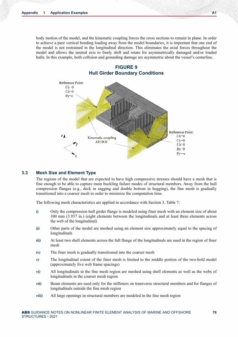
body motion of the model, and the kinematic coupling forces the cross sections to remain in plane. In orderto achieve a pure vertical bending loading away from the model boundaries, it is important that one end ofthe model is not restrained in the longitudinal direction. This eliminates the axial forces throughout themodel and allows the neutral axis to freely shift and rotate for asymmetrically damaged and/or loadedhulls. In this example, both collision and grounding damage are asymmetric about the vessel’s centerline.

FIGURE 9Hull Girder Boundary Conditions

3.3 Mesh Size and Element TypeThe regions of the model that are expected to have high compressive stresses should have a mesh that isfine enough to be able to capture main buckling failure modes of structural members. Away from the hullcompression flanges (e.g., deck in sagging and double bottom in hogging), the fine mesh is graduallytransitioned into a coarser mesh in order to minimize the computation time.

The following mesh characteristics are applied in accordance with Section 3, Table 7:

i) Only the compression hull girder flange is modeled using finer mesh with an element size of about100 mm (3.937 in.) (eight elements between the longitudinals and at least three elements acrossthe web of the longitudinal)

ii) Other parts of the model are meshed using an element size approximately equal to the spacing oflongitudinals

iii) At least two shell elements across the full flange of the longitudinals are used in the region of finermesh

iv) The finer mesh is gradually transitioned into the coarser mesh

v) The longitudinal extent of the finer mesh is limited to the middle portion of the two-hold model(approximately five web frame spacings)

vi) All longitudinals in the fine mesh region are meshed using shell elements as well as the webs oflongitudinals in the coarser mesh region

vii) Beam elements are used only for the stiffeners on transverse structural members and for flanges oflongitudinals outside the fine mesh region

viii) All large openings in structural members are modeled in the fine mesh region



76

All quadrilateral shell elements are first-order full integration general purpose elements (S4) applicable tosmall and finite strains and thick and thin plates. The usage of triangular shell elements is minimized,especially in the fine mesh region. Timoshenko beam elements (B31) are used for the stiffeners ontransverse structural members and for flanges of longitudinals outside the fine mesh region.

3.4 Damage ExtentCollision and grounding damage are considered as two separate cases. Damage is assumed to have arectangular shape with transverse dimensions similar to the ones specified for collision and grounding in[19]. Appendix 1, Figure 10 shows schematically the transverse damage extent for the bulk carrier. Thecollision and grounding damage extents are shown on the same figure for simplicity only. The groundingdamage is positioned so that it includes the bilge, thus creating the greatest amount of geometricasymmetry. The grounding damage reaches three quarters of the double bottom height, leaving only theinner bottom plating with its longitudinals.

In the longitudinal direction, the collision and grounding damage spans three web frame spacings,including the transverse structure at the ends of the damage extent. The ends of the damage include sharpstress concentration raisers that are left on purpose in the FE models to simulate stress concentrations inthe real-world damage case.

FIGURE 10Damage Extent

3.5 Analysis TypeResults are obtained using explicit quasi-static analysis with reversed mass scaling where the density of thematerial is reduced by an order of magnitude to minimize the inertial effects. Explicit analysis is selectedbecause it is very effective on large systems.

The curvature is applied using a Smooth Step amplitude option in Abaqus (see 3/5.3). This minimizes theinertial effect at the beginning of the analysis by gradually increasing the curvature application rate.Curvature application time is one second.

The relatively small number of beam elements in the model governs the critical time increment of theexplicit analysis. Therefore, selective subcycling is used to decrease the computation time, as stated in3/5.2.2.



77

Nonlinear geometry is considered in all analyses using NLGEOM = on in Abaqus. Also, double precisionis used for the analysis and the packager (preprocessor).

A small amount of viscous damping should be introduced when running explicit analysis to control highfrequency oscillations. In Abaqus, this is achieved by specifying linear and quadratic bulk viscosityparameters. The default values are 0.06 and 1.2, respectively, and are considered suitable for most types ofanalysis.

3.6 ResultsAppendix 1, Figure 11 shows the moment curvature (load-displacement) plots for the sagging and hoggingconditions of the intact and damaged structure. It is seen how the collision and grounding damage decreasethe ultimate strength of the hull girder.

Appendix 1, Figure 12 shows the interframe collapse mode of the intact bulk carrier in the hoggingcondition. Interframe collapse mode is very common for intact ship structures.

Appendix 1, Figure 13 shows the non-interframe collapse mode of the bulk carrier with the groundingdamage in hogging. It is seen that the entire inner bottom on the damaged side has buckled due to the lackof the primary support members such as floors and longitudinal girders. The intact side of the doublebottom experiences the interframe collapse.

Appendix 1, Figure 14 shows the collapse mode of the bulk carrier with collision damage in sagging. It isseen how the interframe collapse mechanism originates at the sharp corner of the damage in the decksubjected to compressive loads.

In order to verify that the quasi-static stable response is obtained using explicit analysis, the ratio of kinetic(ALLKE) and internal strain energies (ALLIE) is plotted for all analyses in Appendix 1, Figure 15. Exceptat the beginning of each analysis, the ratio of energies stays below the 5% threshold, as stated in 3/5.2.2and 3/5.3. It is also a good practice to check the behavior of the structure at the beginning of the analysisby comparing the response of the NLFEA with the response of a purely linear analysis. This is shown inAppendix 1, Figure 16 for the case of the intact bulk carrier in hogging. It is seen that a stable quasi-staticresponse is achieved at the beginning of the analysis as well.



78

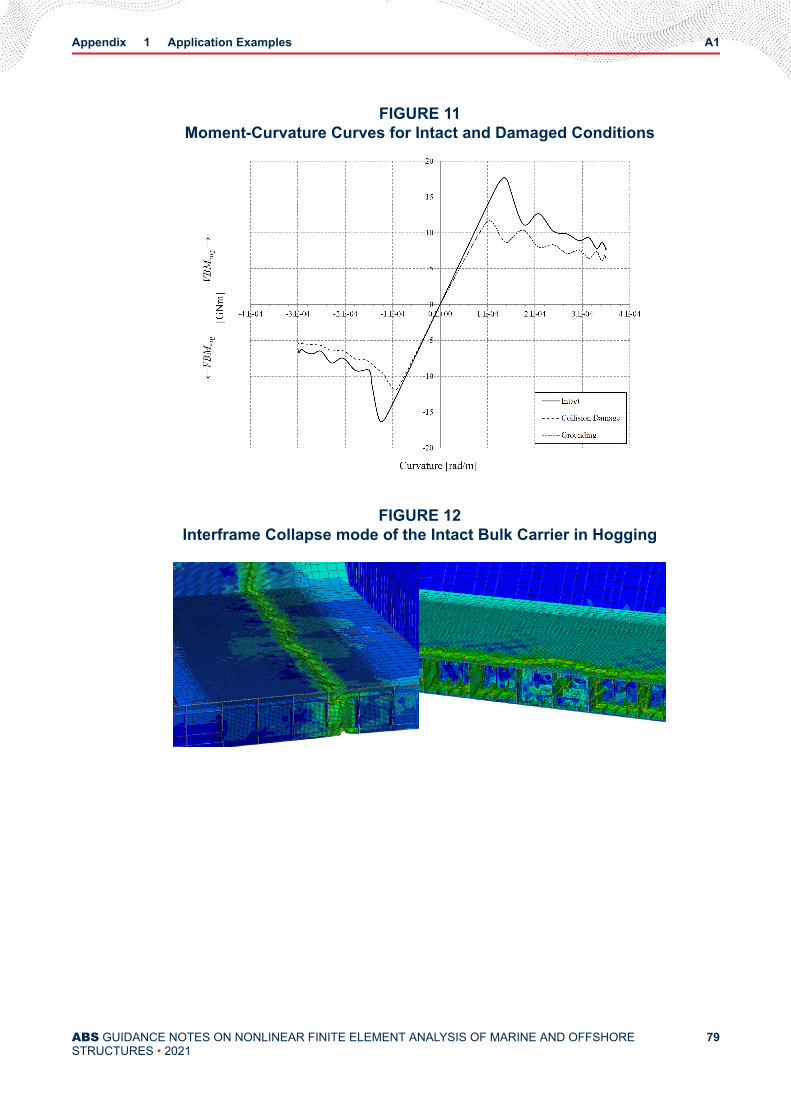
FIGURE 11Moment-Curvature Curves for Intact and Damaged Conditions

FIGURE 12Interframe Collapse mode of the Intact Bulk Carrier in Hogging



79

FIGURE 13Collapsed Bulk Carrier with Grounding Damage in Hogging

FIGURE 14Collapsed Bulk Carrier with Collision Damage in Sagging



80

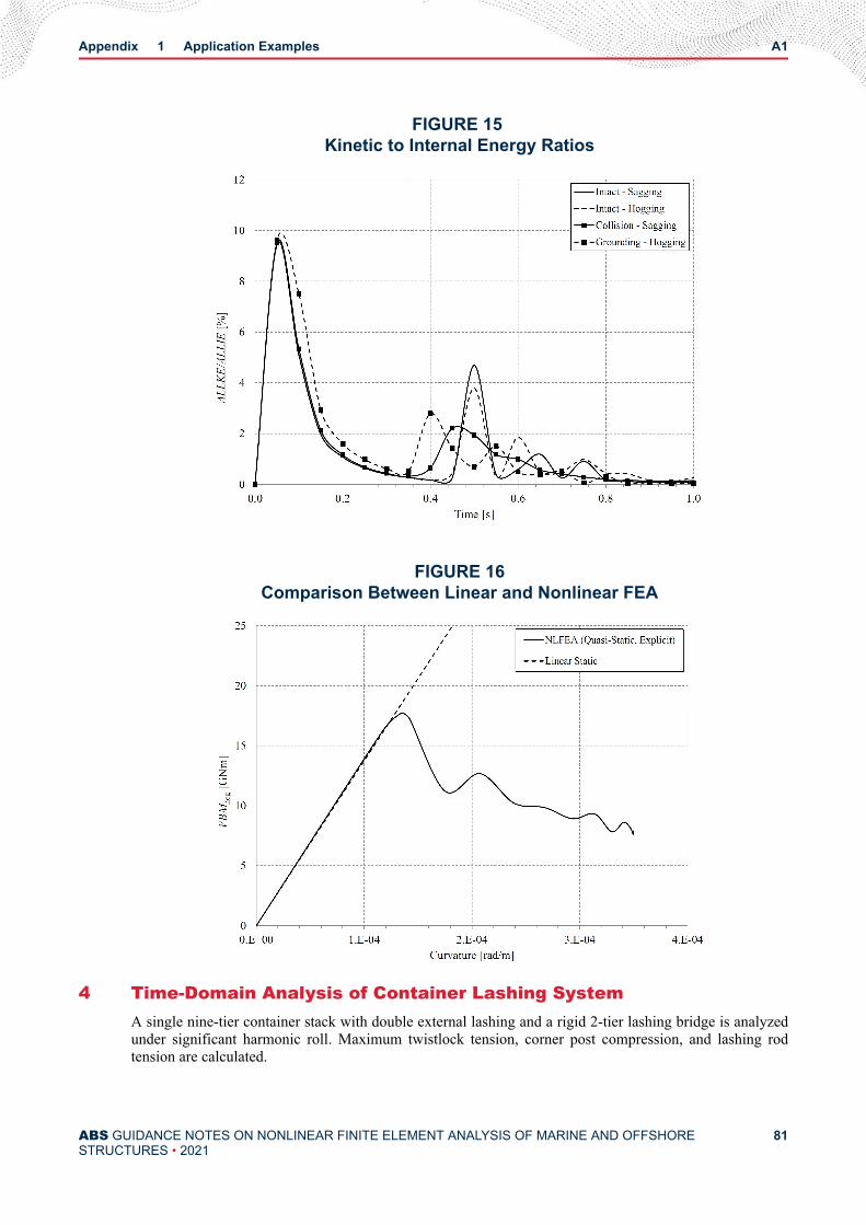
FIGURE 15 Kinetic to Internal Energy Ratios

FIGURE 16Comparison Between Linear and Nonlinear FEA

4 Time-Domain Analysis of Container Lashing SystemA single nine-tier container stack with double external lashing and a rigid 2-tier lashing bridge is analyzedunder significant harmonic roll. Maximum twistlock tension, corner post compression, and lashing rodtension are calculated.



81

Tall container stacks exhibit strong nonlinear behavior caused primarily by:

i) Container corner separations (containers can separate without any resistance until the twistlockclearance value is exhausted and the twistlock engages)

ii) Inability of the lashing rod to carry compressive loads

iii) Coupling between the overturning moment about the base of the stack and the relative transversedeformation of the stack caused mainly by the container corner separations on the tension side ofthe stack and the resulting container rigid body rotations

Material nonlinearity does not significantly affect the stack forces up to their allowable limits and does notneed to be considered in nonlinear static or time-domain analyses.

4.1 Container Stack ModelingAll nine containers are standard International Organization for Standardization (ISO) 40 feet high cubecontainers.

4.1.1 TwistlocksThe containers are mutually connected with twistlocks. Fully automatic twistlocks (FATs) are usedabove the highest lashing point, and semi-automatic twistlocks (SATs) are used below the highestlashing point. Twistlocks are modeled in Abaqus using Cartesian Connectors with prescribedclearance (gap) values in all three directions (see Appendix 1, Table 2). Appendix 1, Figure 17shows the nonlinear force-separation behavior of the twistlocks. Friction in the twistlocks is alsomodeled using Coulomb’s Law.

TABLE 2Twistlock Clearances

Clearance mm (in.)

Vertical Transverse Longitudinal

FAT 0-30 (0-1.181) ± 0.75 (± 0.030) ± 4 (± 0.157)

SAT 0-12 (0-0.472) ± 0.75 (± 0.030) ± 4 (± 0.157)



82

FIGURE 17Nonlinear Behavior of Twistlocks

4.1.2 Lashing RodsThe container stack is secured to the 1-tier lashing bridge with the double external lashing patternthat connects the bottom container corners of the third tier and top container corners of the secondtier with the top platform of the lashing bridge, as can be seen in Appendix 1, Figure 19. Lashingrods are modeled as nonlinear springs having almost zero stiffness in compression and linearstiffness in tension. The lashing rod stiffness in tension is determined based on the lashing roddiameter, length, and the effective modulus of elasticity, as specified in the ABS Guide forCertification of Container Securing Systems. Appendix 1, Figure 18 shows the nonlinear behaviorof the lashing rod when transitioning from tension to compression.



83

FIGURE 18Nonlinear Behavior of Lashing Rods

4.1.3 Container Masses and Mass Proportional DampingContainer cargo is modeled as a point mass located in the middle of the container in thelongitudinal and transverse directions and at 45% of the container height. The cargo massmoments of inertia are specified under the assumption of a homogeneous mass distribution insidethe container up to 90% of the container height. The cargo mass is then connected usingDistributed Continuum coupling to all four corners of the container so that it can follow themotion of the container in an average sense. The cargo mass and the container structural mass givethe total mass of the loaded container which can be seen in Appendix 1, Figure 19 for each tier.

Mass proportional damping from the Rayleigh damping model is specified for container cargo andstructural masses. The damping coefficient α is calibrated based on measurement data for a similarnine tier stack with double external lashing.

4.2 Boundary Conditions and LoadsHarmonic rolling is prescribed at the instantaneous center of roll (COR) of the vessel. All other DOF arefixed at the COR, which is then kinematically coupled with the twistlocks at the bottom of the stack andwith the bottom ends of each lashing rod, as shown in Appendix 1, Figure 19.

Gravity is first applied in a separate step of the analysis over a time period of two seconds using SmoothStep function to avoid numerical issues and noise in the results.

In the next step, harmonic roll with an amplitude of 14° and a period of 26 seconds is applied as a timeseries of prescribed roll motion at the COR of the vessel. Five full roll cycles are analyzed. The rollamplitude is gradually increased from 0° to 14° over the first 26 seconds of the analysis in order to avoidnumerical issues at the start of the analysis and results that have too much noise. Appendix 1, Figure 20shows the time history of applied roll motion at the COR.



84

FIGURE 19Container Stack Modeling

FIGURE 20Time History of Applied Roll Motion at COR

The prescribed roll motion time series is entered tabularly into Abaqus. Care should be taken that the inputtime series is smooth enough, since the tabular data will be linearly interpolated and will not havecontinuous first derivatives. If a time derivative of the input time series is required (e.g., in order to getvelocity and acceleration from a prescribed displacement), and if the resolution of the input time series iscoarse, this can create a substantial amount of noise in the results. In this case, smoothing of the input timeseries should be used. Abaqus applies quadratic smoothing across a fraction of the time intervals beforeand after each point of the input time series. A fraction value equal to 0.05 is recommended when input



85

time series are coarse. In this example, the input roll time series interval is very small (1 ms), and thesmoothing does not have a big impact.

When performing dynamic analysis, attention should be paid to the sampling frequency of the response(frequency at which the results are saved). If this frequency is less than twice the highest frequencyexpected in the response of the structure, then aliasing will occur, meaning that the time series of theresults will not be completely defined, and loss of information and distortion of the time series will occur.In this example, a sampling frequency of 23 Hz is used, which is sufficient since the highest expectedrelevant frequency is about 5 Hz. Anything above 5 Hz can be considered as numerical noise and can befiltered out. In this example, time series of the results are filtered using the Butterworth filter with a cutofffrequency of 5 Hz. The amount of noise present in the results is found to be very small, however.

4.3 Mesh Size and Element TypeEach container is constructed using only Timoshenko beam elements (B31) with one element per containeredge. Beam General Section is used in Abaqus to directly define the cross-sectional properties of eachelement (cross-sectional area, moments of inertia, torsion constant, modulus of elasticity, Poisson ratio,density, damping, and transverse shear). All these properties are calibrated so that the container hasmatching racking stiffness constants on all sides as required by the ABS Guide for Certification ofContainer Securing Systems. This modeling technique enables an adequate simulation of the containerglobal structural response without the need for modeling the container corrugated plating.

4.4 Analysis Type Explicit time-domain nonlinear analysis is used to determine the response of the container stack toharmonic roll motion. This type of analysis has proven very effective in simulating the dynamic behaviorof container stacks, especially when multiple stacks, even whole bays, are modeled and the contactbetween containers is simulated. Also, twistlock and lashing rod failure can be simulated, which may leadto stack collapse and loss of containers.

Nonlinear geometry is considered using NLGEOM = on in Abaqus. Also, double precision is used for theanalysis and the packager (preprocessor).

A small amount of viscous damping should be introduced when running explicit analysis to control highfrequency oscillations. In Abaqus, this is achieved by specifying linear and quadratic bulk viscosityparameters. The default values are 0.06 and 1.2, respectively, and are considered suitable for most types ofanalysis.

4.5 ResultsTime series of maximum twistlock tension, corner post compression, and lashing rod tension occurring inthe stack are given in Appendix 1, Figure 21, Figure 22, and Figure 23, respectively. It is seen that all forcetime series exhibit a periodic, albeit not harmonic, response, which is a characteristic of a nonlinearsystem. Since the roll amplitude is slowly ramped up during the first roll cycle, the results reach a steadystate during the second cycle. Another feature common to all the results is the local vibratory response ofthe stack as it rolls over to one side. This is evident in the oscillations of the time series around the peakvalues.

Appendix 1, Figure 21 shows the time series with the maximum twistlock tension of 247.8 kN (25.27 tf,24.87 Ltf) (positive twistlock force) which occurs in the first FAT above the highest lashing point. This isvery common since this is the first twistlock unprotected by the lashing rods with all the above containerspulling on it. The twistlock separation time series is also plotted on the same graph. It is seen that thetension force in the twistlock only exists when the maximum twistlock clearance of 20 mm (0.787 in.) isexhausted and the twistlock engages.

Appendix 1, Figure 22 shows the maximum corner post compression of 715.7 kN (72.98 tf, 71.83 Ltf). Itoccurs in tier-2 container, which is also common for this type of lashing pattern and lashing bridge height.



86

Corner post compression is calculated by combining the top corner twistlock force with the verticalcomponent of the lashing rod tension attached to the same container corner, if present. Care should betaken regarding signs of the forces when combining the two time series.

FIGURE 21Maximum Twistlock Tension (TT)

FIGURE 22Maximum Corner Post Compression (CPC)

Appendix 1, Figure 23 shows two lashing rod tension time series: the maximum lashing rod tension amongall upper lashing rods (rods connecting the bottom container corners of the third tier with the lashingbridge) and the maximum lashing rod tension among all lower lashing rods (rods connecting the topcontainer corners of the second tier with the lashing bridge). Due to the separation of the corners betweenthe upper and lower lashing rods, caused by the twistlock clearance, the upper lashing rod will have largerelongation, and thus, larger tensile forces. Maximum tension in the upper lashing rods is 233.9 kN (23.85tf, 23.47 Ltf) and the maximum tension in the lower lashing rods is 89.0 kN (9.08 tf, 8.93 Ltf). Linearanalysis cannot account for the twistlock clearance and thus predicts equal forces in both lashing rods. It isalso seen in Appendix 1, Figure 23 that there is no compression force in the lashing rods due to thespecified nonlinear behavior of the lashing rods. The maximum upper and lower lashing rod tension forcesoccur on the opposite sides of the container (port side and starboard side). This is why the two time seriesare out of phase.



87

FIGURE 23Maximum Lashing Rod Tension (LRT)

In the absence of twistlock clearances, the container stack will deform, relative to its base, only due tocontainer racking, and these transverse deformations are generally small. However, twistlock clearancesenable additional rigid body rotation of each container, and this causes the container stack to significantlydeform relative to its base. Such significant deformation causes coupling between the overturning momentabout the base of the stack and the relative transverse deformation of the stack. As the stack deforms, themoment around the base of the stack increases. This effect cannot be captured by linear stack analysis.Appendix 1, Figure 24 shows the maximum relative stack deformation of the stack at the instant of largestroll angle. The stack is shown such that its base is in the horizontal position, and its roll angle is indicatedin Appendix 1, Figure 24 by the orientation of the coordinate system.



88

FIGURE 24Relative Transverse Deformation of the Stack

5 Indentation of a Stiffened Panel (2021)This example demonstrates the use of NLFEA to analyze the impact between a stiffened panel and arounded rigid indenter causing plastic deformation and ductile fracture of the stiffened panel. The problemis treated dynamically. Strain-rate hardening is simulated using the Cowper-Symonds mode, in accordancewith 3/9.5. The fracture is also modeled using the linear damage accumulation law with the Liu ductilefracture criteria described in 3/11.

5.1 Geometry and Material (2021)The stiffened panel geometry is shown in Appendix 1, Figure 25 and the panel particulars are given inAppendix 1, Table 3. The stiffened panel is impacted by a small semi-spherical indenter with a radius r =300 mm (11.811 in.) and a mass of 12 t (26455.5 lb) from the unstiffened side. The indenter is placed inthe middle of the model between the stiffeners. At the beginning of the analysis, the top of the indenter isone millimeter away from the plate, including the thickness of the plate. This is done to avoid initialcontact overclosures.



89

FIGURE 25Model Geometry and Boundary Conditions (2021)

TABLE 3Model Geometry Parameters

Dimension Value mm (in.) DescriptionA 3000 (118.110) Overall panel lengthB 4050 (159.449) Overall panel breadthb 810 (31.890) Stiffener spacingℎw 150 (5.906) Height of webbf 90 (3.543) Breadth of flangetp 6 (0.236) Thickness of platetw 9 (0.354) Thickness of webtf 9 (0.354) Thickness of flanger 300 (11.811) Radius of the indenter

Material of the panel is HS32 steel with parameters described in Section 3, Table 4. Since there are no loadreversals or cyclic loads, isotropic hardening model is used. Strain rate hardening is simulated using theCowper-Symonds model, which for high tensile steels has C = 3200 s-1 and q = 5, in accordance withrecommended values from Section 3, Table 5. In Abaqus, this is selected as the Power Law Rate Dependedhardening suboption of the Plastic material behavior with Multiplier = 3200 and Exponent = 5.

In this example, Liu ductile fracture criteria [20] is used. This criterion is of the form given by Eq. 3.31with a constant critical fracture strain for a certain element size and plate thickness. The Liu criterion isgiven in Eq. A1.2, which also shows how the criterion is modeled in Abaqus using the Johnson-Cooklinear damage accumulation law (only available for explicit analysis):εcf = 0.5 – 0.01Ltd1 = 0.5 – 0.01Lt = 0.5 – 0.01306 = 0.45 . . . . . . . . . . . . . . . . . . . . . . . . . . . . . . . . . . . (A1 . 2)d2 = d3 = d4 = d5 = 0



90

as explained in 3/11, where L = 30 mm (1.181 in.) is the size of the stiffened panel plate elements and t = 6mm (0.236 in.) is the plate thickness. As described in [12], the Liu criterion is particularly suitable forsimulating penetrations with a rounded indenter, such as the one used in this example. The criterion is validfor L/t in the range from 5 to 20 for mild and high tensile steels. The Liu criterion assumes there is noductile fracture evolution. In Abaqus, this is modeled using Displacement at failure = 0 in the DamageEvolution suboption of the Johnson-Cook Damage material behavior.

No initial imperfections are modeled, as they have a negligible impact on this kind of analysis.

5.2 Boundary Conditions and Loads (2021)All edges of the panel are clamped, as can be seen in Appendix 1, Figure 25. This is a conservativeassumption. In a real case scenario (e.g., object dropped onto a deck of a vessel), the edges of the panelwill be allowed to deform, and the energy of the impact will be absorbed by a larger part of the deckstructure.

The indenter has an initial velocity of 12 m/s (39.37 ft/s) in the z direction perpendicular to the stiffenedpanel plate (see Appendix 1, Figure 25). There are no other externally applied loads. Therefore, once thesimulation starts, the energy of the system remains constant, and the initial kinetic energy of the indenter ismainly transformed into the internal strain energy of the stiffened panel. A part of the initial kinetic energyis dissipated through friction, contact, ductile fracturing, and bulk viscous dissipation. As the kineticenergy of the indenter is transformed into the internal energy of the stiffened panel or dissipated, theindenter slows down. The analysis is run for one second, during which the indenter penetrates through thestiffened panel and continues moving in the same direction at a significantly reduced speed.

5.3 Mesh Size and Element TypeThe entire stiffened panel is meshed using first-order shell quadrilaterals with full integration (S4). Theseare general purpose shell elements applicable to small and finite strains and thick and thin plates.

A uniform mesh size of 30 mm (1.181 in.) is used with an element side ratio equal to one for all elements.The mesh size was selected to be 5t, where t = 6 mm (0.236 in.) is the plate thickness. This is the finestmesh admissible by the Liu ductile fracture criteria, as noted in 3/11.

A rigid semi-spherical indenter is meshed using R3D4 bilinear rigid quadrilaterals and a small number ofR3D3 linear rigid triangles. Mesh size for the indenter is also 30 mm (1.181 in.). This enables a smoothcontact.

5.4 Contact ModelingThe General contact algorithm is used to model contact between the indenter and the stiffened panel,where Abaqus assigns the contact pairs automatically, including the self-contact.

The Hard Contact pressure-overclosure relationship is used in the normal direction with the Penaltyconstraint enforcement method.

Frictional behavior is specified in the tangential direction using the Penalty frictional formulation with acoefficient of friction equal to 0.3.

5.5 Analysis TypeExplicit dynamic analysis is performed. Nonlinear geometry is considered using NLGEOM = on. A smallamount of viscous damping should be introduced when running explicit analysis to control high frequencyoscillations. In Abaqus, this is achieved by specifying linear and quadratic bulk viscosity parameters. Thedefault values are 0.06 and 1.2, respectively, and are considered suitable for most types of analysis.



91

5.6 Results (2021)Appendix 1, Figure 26 shows the distribution of the equivalent plastic strain, εp (PEEQ in Abaqus), on apunctured stiffened panel at the end of the analysis. As soon as the equivalent plastic strain reaches thefracture limit (PEEQ = 0.45) at all through thickness sections of a shell element on at least one integrationpoint, the element is deleted, and the fracture occurs. This is clearly indicated in Appendix 1, Figure 26,where the maximum contour of PEEQ is 0.45 and occurs close to the rim of the fracture.

FIGURE 26Equivalent Plastic Strain Distribution on a Punctured Stiffened Panel (2021)

Appendix 1, Figure 26 also shows the areas with permanent plastic deformation (PEEQ > 0). At the end ofthe analysis, the elastic strains are recovered, and the small vibrations of the panel caused by a suddenimpact are faded.

The average displacement of the plate in the z direction around the fracture (not including the jagged edgesof the puncture) is approximately equal to 300 mm (11.811 in.). Using Eq. 3.17, the strain rate can beestimated at 20 s-1. At this strain rate, the hardening effect on the material flow curve will be significant.The relationship between the dynamic and static true flow curves can be obtained by using Eq. 3.16: σ ε dyn = 1.36σ ε ........................................................................................................................... (A1.3)

where σ ε dyn is the dynamic true flow curve and σ(ε) is the static true flow curve. Therefore, thedynamic yield stress is 36% greater than the static yield stress.

Appendix 1, Figure 27 shows plots of the energy absorbed by the stiffened panel (internal astrain energyALLIE) over time. Cases with and without the strain rate effect are shown. The initial kinetic energy of theindenter is 0.864 MJ. It is seen that about 92.4% of that kinetic energy is absorbed by the stiffened panelwhen strain rate hardening effect is considered. When it is not considered, only 57.6% of the initial kineticenergy of the indenter is absorbed by the stiffened panel.



92

6 Impact with IceFor an example of the application of NLFEA to analyze the impact of vessel’s side structure with ice, seethe ABS Guidance Notes on Ice Class.

FIGURE 27Absorbed Energy Over Time (2021)



93

A P P E N D I X 2Tabulated True Flow Curves

TABLE 1Steel Grades MS, HS32, HS36

MS HS32 HS36

TrueStrain

ε[%]

True PlasticStrain

εp=ε-σ/E[%]

TrueStress

σ[N/mm2]

TrueStrain

ε[%]

True PlasticStrain

εp=ε-σ/E[%]

TrueStress

σ[N/mm2]

TrueStrain

ε[%]

True PlasticStrain

εp=ε-σ/E[%]

TrueStress

σ[N/mm2]

0.000 0.000 0.000 0.000 0.000 0.000 0.000 0.000 0.000

0.112 0.000 235.263 0.150 0.000 315.473 0.169 0.000 355.600

0.456 0.344 236.074 0.485 0.334 316.530 0.499 0.329 356.775

0.800 0.688 236.888 0.819 0.668 317.592 0.829 0.659 357.955

1.145 1.032 237.705 1.154 1.003 318.657 1.159 0.988 359.138

1.489 1.375 238.525 1.489 1.337 319.725 1.489 1.318 360.325

1.861 1.744 245.974 1.861 1.705 328.349 1.861 1.685 369.970

2.233 2.113 253.499 2.233 2.073 337.061 2.233 2.053 379.713

2.606 2.481 261.102 2.606 2.441 345.858 2.606 2.420 389.551

2.978 2.850 268.781 2.978 2.809 354.733 2.978 2.788 399.473

3.878 3.742 287.661 3.878 3.700 376.322 3.878 3.677 423.558

4.779 4.633 306.820 4.779 4.591 397.021 4.779 4.567 446.402

5.680 5.525 325.823 5.680 5.483 414.730 5.680 5.459 465.522

6.581 6.417 343.841 6.581 6.377 428.375 6.581 6.353 480.019

7.481 7.310 359.896 7.481 7.273 438.962 7.481 7.248 491.330

8.382 8.205 373.450 8.382 8.169 447.952 8.382 8.144 501.090

9.283 9.100 384.704 9.283 9.066 456.254 9.283 9.041 510.216

10.184 9.996 394.290 10.184 9.963 464.304 10.184 9.937 519.131

11.084 10.893 402.841 11.084 10.860 472.301 11.084 10.834 528.024

11.985 11.790 410.813 11.985 11.757 480.338 11.985 11.730 536.980


94

MS HS32 HS36

TrueStrain

ε[%]

True PlasticStrain

εp=ε-σ/E[%]

TrueStress

σ[N/mm2]

TrueStrain

ε[%]

True PlasticStrain

εp=ε-σ/E[%]

TrueStress

σ[N/mm2]

TrueStrain

ε[%]

True PlasticStrain

εp=ε-σ/E[%]

TrueStress

σ[N/mm2]

12.886 12.687 418.491 12.886 12.654 488.463 12.886 12.627 546.044

13.787 13.584 426.044 13.787 13.551 496.700 13.787 13.523 555.239

14.687 14.481 433.572 14.687 14.447 505.063 14.687 14.419 564.578

15.588 15.378 441.135 15.588 15.344 513.561 15.588 15.316 572.641

16.489 16.276 448.767 16.489 16.242 518.785 16.489 16.215 577.584

17.390 17.173 456.493 17.390 17.141 523.147 17.390 17.113 582.303

18.290 18.070 464.328 18.290 18.040 527.321 18.290 18.012 586.819

19.191 18.967 472.283 19.191 18.939 531.326 19.191 18.910 591.150

20.092 19.863 480.364 20.092 19.838 535.176 20.092 19.809 595.313

20.993 20.760 488.578 20.993 20.737 538.883 20.993 20.708 599.321

21.893 21.657 496.931 21.893 21.636 542.458 21.893 21.607 603.185

22.794 22.555 502.353 22.794 22.535 545.911 22.794 22.506 606.917

23.695 23.454 506.677 23.695 23.434 549.251 23.695 23.405 610.526

24.596 24.353 510.874 24.596 24.333 552.486 24.596 24.304 614.021

25.496 25.251 514.954 25.496 25.232 555.623 25.496 25.203 617.409

26.397 26.150 518.923 26.397 26.132 558.667 26.397 26.102 620.697

27.298 27.049 522.788 27.298 27.031 561.625 27.298 27.001 623.891

28.199 27.948 526.555 28.199 27.930 564.502 28.199 27.901 626.997

29.099 28.847 530.229 29.099 28.830 567.303 29.099 28.800 630.021

30.000 29.746 533.815 30.000 29.729 570.031 30.000 29.699 632.966

TABLE 2Steel Grades HS40, HS43, HS47

HS40 HS43 HS47

TrueStrain

ε[%]

True PlasticStrain

εp=ε-σ/E[%]

TrueStress

σ[N/mm2]

TrueStrain

ε[%]

True PlasticStrain

εp=ε-σ/E[%]

TrueStress

σ[N/mm2]

TrueStrain

ε[%]

True PlasticStrain

εp=ε-σ/E[%]

TrueStress

σ[N/mm2]

0.000 0.000 0.000 0.000 0.000 0.000 0.000 0.000 0.000

0.186 0.000 390.724 0.200 0.000 420.840 0.219 0.000 461.008

0.511 0.325 391.999 0.522 0.322 422.198 0.536 0.317 462.474

0.837 0.650 393.279 0.844 0.643 423.561 0.854 0.634 463.944

1.163 0.976 394.562 1.167 0.965 424.928 1.171 0.950 465.420

Appendix 2 Tabulated True Flow Curves A2


95

HS40 HS43 HS47

TrueStrain

ε[%]

True PlasticStrain

εp=ε-σ/E[%]

TrueStress

σ[N/mm2]

TrueStrain

ε[%]

True PlasticStrain

εp=ε-σ/E[%]

TrueStress

σ[N/mm2]

TrueStrain

ε[%]

True PlasticStrain

εp=ε-σ/E[%]

TrueStress

σ[N/mm2]

1.489 1.301 395.850 1.489 1.286 426.300 1.489 1.267 466.900

1.861 1.668 406.116 1.861 1.654 437.172 1.861 1.634 478.728

2.233 2.036 416.486 2.233 2.021 448.152 2.233 2.000 490.673

2.606 2.403 426.951 2.606 2.387 459.224 2.606 2.367 502.707

2.978 2.770 437.482 2.978 2.754 470.323 2.978 2.733 514.723

3.878 3.659 462.576 3.878 3.643 495.987 3.878 3.621 541.755

4.779 4.549 484.478 4.779 4.534 516.166 4.779 4.513 561.513

5.680 5.442 500.666 5.680 5.428 530.013 5.680 5.407 574.908

6.581 6.337 512.583 6.581 6.324 540.768 6.581 6.303 585.860

7.481 7.233 522.601 7.481 7.220 550.517 7.481 7.198 596.150

8.382 8.130 531.956 8.382 8.116 560.017 8.382 8.094 606.332

9.283 9.026 541.134 9.283 9.013 569.520 9.283 8.990 616.583

10.184 9.922 550.324 10.184 9.909 579.121 10.184 9.886 626.967

11.084 10.819 559.605 11.084 10.805 588.858 11.084 10.782 636.811

11.985 11.715 569.014 11.985 11.701 597.469 11.985 11.680 642.286

12.886 12.611 578.568 12.886 12.600 602.572 12.886 12.579 647.405

13.787 13.509 585.317 13.787 13.498 607.369 13.787 13.477 652.216

14.687 14.407 590.229 14.687 14.397 611.898 14.687 14.376 656.754

15.588 15.306 594.887 15.588 15.296 616.187 15.588 15.274 661.051

16.489 16.204 599.316 16.489 16.194 620.263 16.489 16.173 665.132

17.390 17.103 603.541 17.390 17.093 624.147 17.390 17.072 669.019

18.290 18.002 607.579 18.290 17.992 627.857 18.290 17.971 672.731

19.191 18.901 611.449 19.191 18.891 631.410 19.191 18.870 676.284

20.092 19.800 615.164 20.092 19.790 634.818 20.092 19.769 679.691

20.993 20.699 618.737 20.993 20.690 638.094 20.993 20.668 682.964

21.893 21.598 622.179 21.893 21.589 641.248 21.893 21.568 686.115

22.794 22.497 625.501 22.794 22.488 644.289 22.794 22.467 689.153

23.695 23.396 628.710 23.695 23.388 647.226 23.695 23.366 692.085

24.596 24.296 631.816 24.596 24.287 650.067 24.596 24.266 694.920

25.496 25.195 634.824 25.496 25.186 652.817 25.496 25.165 697.664

26.397 26.094 637.741 26.397 26.086 655.482 26.397 26.065 700.323

27.298 26.994 640.573 27.298 26.985 658.068 27.298 26.964 702.902



96

HS40 HS43 HS47

TrueStrain

ε[%]

True PlasticStrain

εp=ε-σ/E[%]

TrueStress

σ[N/mm2]

TrueStrain

ε[%]

True PlasticStrain

εp=ε-σ/E[%]

TrueStress

σ[N/mm2]

TrueStrain

ε[%]

True PlasticStrain

εp=ε-σ/E[%]

TrueStress

σ[N/mm2]

28.199 27.893 643.326 28.199 27.885 660.580 28.199 27.864 705.407

29.099 28.792 646.002 29.099 28.784 663.023 29.099 28.763 707.841

30.000 29.692 648.608 30.000 29.684 665.399 30.000 29.663 710.209


HS51 HS56 HS63

TrueStrain

ε[%]

True PlasticStrain

εp=ε-σ/E[%]

TrueStress

σ[N/mm2]

TrueStrain

ε[%]

True PlasticStrain

εp=ε-σ/E[%]

TrueStress

σ[N/mm2]

TrueStrain

ε[%]

True PlasticStrain

εp=ε-σ/E[%]

TrueStress

σ[N/mm2]

0.000 0.000 0.000 0.000 0.000 0.000 0.000 0.000 0.000

0.238 0.000 501.190 0.262 0.000 551.440 0.295 0.000 621.830

0.551 0.312 502.760 0.568 0.306 553.135 0.593 0.298 623.690

0.863 0.624 504.335 0.875 0.612 554.835 0.892 0.595 625.554

1.176 0.936 505.915 1.182 0.918 556.540 1.190 0.893 627.424

1.489 1.248 507.500 1.489 1.224 558.250 1.489 1.191 629.300

1.861 1.614 520.302 1.861 1.590 572.327 1.861 1.555 645.172

2.233 1.980 533.227 2.233 1.955 586.540 2.233 1.920 661.175

2.606 2.346 546.234 2.606 2.321 600.840 2.606 2.285 677.057

2.978 2.712 559.151 2.978 2.686 615.033 2.978 2.650 691.970

3.878 3.600 587.219 3.878 3.572 645.748 3.878 3.538 717.836

4.779 4.491 606.351 4.779 4.463 666.542 4.779 4.432 733.335

5.680 5.386 619.522 5.680 5.357 680.899 5.680 5.326 746.507

6.581 6.281 630.847 6.581 6.252 693.305 6.581 6.221 759.394

7.481 7.177 641.762 7.481 7.147 705.288 7.481 7.115 772.379

8.382 8.072 652.669 8.382 8.042 717.270 8.382 8.011 782.886

9.283 8.968 663.692 9.283 8.937 729.384 9.283 8.909 789.308

10.184 9.863 674.876 10.184 9.832 741.677 10.184 9.807 795.180

11.084 10.761 681.297 11.084 10.729 748.271 11.084 10.705 800.593

11.985 11.659 686.788 11.985 11.627 754.262 11.985 11.603 805.616

12.886 12.558 691.920 12.886 12.525 759.862 12.886 12.502 810.302

13.787 13.456 696.739 13.787 13.424 765.120 13.787 13.400 814.696



97

HS51 HS56 HS63

TrueStrain

ε[%]

True PlasticStrain

εp=ε-σ/E[%]

TrueStress

σ[N/mm2]

TrueStrain

ε[%]

True PlasticStrain

εp=ε-σ/E[%]

TrueStress

σ[N/mm2]

TrueStrain

ε[%]

True PlasticStrain

εp=ε-σ/E[%]

TrueStress

σ[N/mm2]

14.687 14.355 701.284 14.687 14.322 770.079 14.687 14.299 818.834

15.588 15.253 705.586 15.588 15.221 774.772 15.588 15.198 822.744

16.489 16.152 709.669 16.489 16.119 779.227 16.489 16.097 826.452

17.390 17.051 713.558 17.390 17.018 783.469 17.390 16.996 829.978

18.290 17.950 717.269 18.290 17.917 787.518 18.290 17.895 833.339

19.191 18.849 720.821 19.191 18.816 791.392 19.191 18.794 836.552

20.092 19.748 724.225 20.092 19.715 795.105 20.092 19.694 839.629

20.993 20.647 727.496 20.993 20.614 798.673 20.993 20.593 842.582

21.893 21.547 730.642 21.893 21.513 802.105 21.893 21.493 845.420

22.794 22.446 733.675 22.794 22.412 805.413 22.794 22.392 848.153

23.695 23.345 736.602 23.695 23.311 808.605 23.695 23.291 850.788

24.596 24.245 739.431 24.596 24.211 811.690 24.596 24.191 853.332

25.496 25.144 742.168 25.496 25.110 814.676 25.496 25.091 855.793

26.397 26.044 744.820 26.397 26.009 817.568 26.397 25.990 858.174

27.298 26.943 747.392 27.298 26.909 820.373 27.298 26.890 860.482

28.199 27.843 749.889 28.199 27.808 823.096 28.199 27.790 862.721

29.099 28.742 752.315 29.099 28.708 825.742 29.099 28.689 864.895

30.000 29.642 754.675 30.000 29.607 828.315 30.000 29.589 867.008


HS70 HS91 HS98

TrueStrain

ε[%]

True PlasticStrain

εp=ε-σ/E[%]

TrueStress

σ[N/mm2]

TrueStrain

ε[%]

True PlasticStrain

εp=ε-σ/E[%]

TrueStress

σ[N/mm2]

TrueStrain

ε[%]

True PlasticStrain

εp=ε-σ/E[%]

TrueStress

σ[N/mm2]

0.000 0.000 0.000 0.000 0.000 0.000 0.000 0.000 0.000

0.328 0.000 692.267 0.423 0.000 893.772 0.456 0.000 964.389

0.618 0.289 694.279 0.689 0.265 896.157 0.714 0.257 966.882

0.908 0.579 696.297 0.956 0.531 898.548 0.972 0.514 969.381

1.199 0.868 698.320 1.222 0.796 900.946 1.231 0.771 971.887

1.489 1.157 700.350 1.489 1.061 903.350 1.489 1.028 974.400

1.861 1.521 718.578 1.861 1.427 916.985 1.861 1.397 982.140



98

HS70 HS91 HS98

TrueStrain

ε[%]

True PlasticStrain

εp=ε-σ/E[%]

TrueStress

σ[N/mm2]

TrueStrain

ε[%]

True PlasticStrain

εp=ε-σ/E[%]

TrueStress

σ[N/mm2]

TrueStrain

ε[%]

True PlasticStrain

εp=ε-σ/E[%]

TrueStress

σ[N/mm2]

2.233 1.884 736.782 2.233 1.793 930.573 2.233 1.765 989.870

2.606 2.248 753.444 2.606 2.159 942.899 2.606 2.134 997.104

2.978 2.615 765.963 2.978 2.527 952.241 2.978 2.503 1003.152

3.878 3.507 783.941 3.878 3.421 967.498 3.878 3.398 1014.885

4.779 4.401 798.169 4.779 4.315 980.857 4.779 4.294 1025.910

5.680 5.295 812.223 5.680 5.210 994.207 5.680 5.190 1036.983

6.581 6.191 822.193 6.581 6.106 1003.488 6.581 6.086 1046.190

7.481 7.089 828.596 7.481 7.003 1011.018 7.481 6.983 1054.040

8.382 7.987 834.312 8.382 7.901 1017.737 8.382 7.880 1061.045

9.283 8.885 839.477 9.283 8.798 1023.808 9.283 8.778 1067.374

10.184 9.784 844.192 10.184 9.697 1029.348 10.184 9.676 1073.150

11.084 10.682 848.530 11.084 10.595 1034.444 11.084 10.574 1078.462

11.985 11.581 852.548 11.985 11.493 1039.164 11.985 11.473 1083.383

12.886 12.480 856.292 12.886 12.392 1043.561 12.886 12.371 1087.968

13.787 13.379 859.798 13.787 13.291 1047.677 13.787 13.270 1092.259

14.687 14.278 863.095 14.687 14.190 1051.548 14.687 14.169 1096.295

15.588 15.178 866.207 15.588 15.089 1055.201 15.588 15.068 1100.104

16.489 16.077 869.155 16.489 15.988 1058.661 16.489 15.967 1103.710

17.390 16.976 871.955 17.390 16.887 1061.947 17.390 16.866 1107.136

18.290 17.876 874.622 18.290 17.786 1065.077 18.290 17.765 1110.399

19.191 18.775 877.168 19.191 18.686 1068.064 19.191 18.664 1113.514

20.092 19.675 879.604 20.092 19.585 1070.923 20.092 19.564 1116.494

20.993 20.575 881.940 20.993 20.485 1073.663 20.993 20.463 1119.350

21.893 21.474 884.184 21.893 21.384 1076.294 21.893 21.363 1122.094

22.794 22.374 886.342 22.794 22.284 1078.826 22.794 22.262 1124.733

23.695 23.274 888.422 23.695 23.183 1081.265 23.695 23.162 1127.276

24.596 24.174 890.428 24.596 24.083 1083.618 24.596 24.061 1129.729

25.496 25.073 892.367 25.496 24.982 1085.891 25.496 24.961 1132.100

26.397 25.973 894.243 26.397 25.882 1088.090 26.397 25.861 1134.392

27.298 26.873 896.059 27.298 26.782 1090.220 27.298 26.760 1136.612

28.199 27.773 897.820 28.199 27.682 1092.284 28.199 27.660 1138.764



99

HS70 HS91 HS98

TrueStrain

ε[%]

True PlasticStrain

εp=ε-σ/E[%]

TrueStress

σ[N/mm2]

TrueStrain

ε[%]

True PlasticStrain

εp=ε-σ/E[%]

TrueStress

σ[N/mm2]

TrueStrain

ε[%]

True PlasticStrain

εp=ε-σ/E[%]

TrueStress

σ[N/mm2]

29.099 28.673 899.529 29.099 28.581 1094.287 29.099 28.560 1140.853

30.000 29.573 901.188 30.000 29.481 1096.233 30.000 29.459 1142.881



100

A P P E N D I X 3References

[1] J. K. Paik and A. K. Thayamballi, Ship–Shaped Offshore Installations: Design, Building, andOperation, Cambridge: Cambridge University Press, 2007.

[2] O. Hughes and J. K. Paik, Ship Structural Analysis and Design, Jersey City, NJ: The Society ofNaval Architects and Marine Engineers, 2010, pp. 8.1-8.22.

[3] N. E. Dowling, Mechanical Behavior of Materials, Third ed., Upper Saddle River, NJ: PearsonPrentice Hall, 2007.

[4] P. Wriggers, Nonlinear Finite Element Methods, Heidelberg: Springer-Verlag, 2008.

[5] M. A. Crisfield, "A fast incremental/iterative solution procedure that handles “snap-through”,"Computers & Structures, vol. 13, no. 1-3, pp. 55-62, 1981.

[6] E. Riks, "An incremental approach to the solution of snapping and buckling problems,"International Journal of Solids and Structures, vol. 15, no. 7, pp. 529-551, 1979.

[7] H. M. Hilber, T. J. R. Hughes and R. L. Taylor, "Improved numerical dissipation for timeintegration algorithms in structural dynamics," Earthquake Engineering and Structural Dynamics,vol. 5, no. 3, pp. 283-292, 1977.

[8] E. Lehmann, "Discussion on Report of Committee III. 1: Ultimate Strength," in Proceedings of16th ISSC, pp. 121–131, 2006.

[9] J. Lubliner, Plasticity Theory, Berkeley, CA: Jacob Lubliner, 2006.

[10] X. Yun and L. Gardner, "Stress-strain curves for hot-rolled steels," Journal of Constructional SteelResearch, vol. 133, pp. 36-46, 2017.

[11] N. Jones and C. Jones, "Inelastic failure of fully clamped beams and circular plates under impactloading," Proceedings of the Institution of Mechanical Engineers, Part C: Journal of MechanicalEngineering Science, vol. 216, no. 2, pp. 133-149, 2002.

[12] S. Zhang, P. T. Pedersen and R. Villavicencio, Probability and Mechanics of Ship Collision andGrounding, Oxford: Butterworth-Heinemann, 2019.

[13] R. Törnqvist, Design of Crashworthy Ship Structures (Phd Thesis), Kongens Lyngby: TechnicalUniversity of Denmark, 2003.

[14] M. Storheim, J. Amdahl and I. Martens, "On the accuracy of fracture estimation in collisionanalysis of ship and offshore structures," Marine Structures, vol. 44, pp. 254-287, 2015.

[15] G. R. Johnson and W. H. Cook, "Fracture characteristics of three metals subjected to variousstrains, strain rates, temperatures and pressures," Engineering Fracture Mechanics, vol. 21, no. 1,pp. 31-48, 1985.


101

[16] J. e. a. Czujko, "Committee III.1 - Ultimate Strength," in Proceedings of the 20th InternationalShip and Offshore Structures Congress, 2018.

[17] Simulia Corp, SIMULIA User Assistance 2018, Providence, RI: Dassault Systèmes Simulia Corp.,2017.

[18] M. Petričić, "Survivability of Hull Girder in Damaged Condition," Ship Structure Committee,Washington, 2015.

[19] IACS, Common Structural Rules for Bulk Carriers and Oil Tankers – External Release 1, London:International Association of Classification Societies, 2014.

[20] B. Liu, R. Villavicencio, S. Zhang and C. Guedes Soares, "A simple criterion to evaluate therupture of materials in ship collision simulations," Marine Structures, vol. 54, pp. 92-111, 2017.

Appendix 3 References A3


102

Nonlinear Finite Element Analysis of Marine and Offshore ...

Documents

Transcript of Nonlinear Finite Element Analysis of Marine and Offshore ...