Noise Momentum Around the World - UQ eSpace

CHARLIE X. CAI, ROBERT FAFF, AND YONGCHEOL SHIN

Noise Momentum Around the World

We argue that arbitrageurs will strategically limit their initial investment inan arbitrage opportunity in anticipation of further mispricing caused by thedeepening of noise traders’ misperceptions. Such ‘noise momentum’ is animportant determinant of the overall arbitrage process. We design anempirical strategy to capture noise momentum in a two-period generalizederror correction model. Applying it to a wide range of internationalspot-futures market pairs, we document pervasive evidence of noisemomentum around the world.

Key words: Futures and spot prices; Initial mispricing correction; Limitedarbitrage; Noise momentum.

Existing empirical studies of the limits to arbitrage focus on the initial mispricingerror correction coefficient in a one-period framework designed to measure thelevel of arbitrage activity. In contrast, the theoretical work of Shleifer and Vishny(SV, 1997) models the arbitrage process in a multi-period setup. In their paper, overand above the error correction component, we identify a theoretical concept(hitherto ignored in the literature) that forms a potentially important part of thedeterminants of the arbitrage process. Specifically, in SV’s model, one of the criticalconsiderations for the arbitrageur in deciding how much effort to apply to correctinginitial mispricing, is the probability of persistence in mispricing. We label thispersistence of the uncorrected pricing errors (after the next period of trading) ‘noisemomentum’. Further, we design an empirical strategy to capture noise momentumin a two-period generalized error correction model (GECM). We execute anempirical application to test the importance of noise momentum across globalmarkets. In so doing, we extend the existing body of knowledge by showing thatnoise momentum, together with the initial unarbitraged pricing error, affects pricemovements and the path to equilibrium. In short, we document empirical evidenceconsistent with the existence of noise momentum around the world.The uncertainty regarding the level of noise trading and the uncertainty of

other arbitrageurs’ actions poses a nontrivial risk to rational arbitrageurs’ activities(see, e.g., Abreu and Brunnermeier, 2002; Kondor, 2004; Stein, 2009). These modelssuggest that knowing the aggregate level of the arbitrage activity present in themarket is important to participants. In contrast to the rich insights offered in existing

CHARLIE X. CAI is Professor of Finance at the University of Leeds, ROBERT FAFF ([email protected]) isProfessor of Finance at the University of Queensland, and YONGCHEOL SHIN is a Professor in the Department ofEconomics and Related Studies at the University of York.

The third author acknowledges partial financial support from the ESRC (Grant No. RES-000-22-3161). The usualdisclaimer applies.

ABACUS, Vol. ••, No. ••, 2017 doi: 10.1111/abac.12101

1© 2017 Accounting Foundation, The University of Sydney

bs_bs_banner

theoretical models on the limits of arbitrage (see Gromb and Vayanos, 2010 for asurvey of the theoretical studies), the short-term dynamics in these models isunder-researched empirically. Our study seeks to redress this situation.To test our hypotheses, we examine the impact of limited arbitrage and noise

momentum in the index futures market, motivated by the ongoing interest in spotand futures price dynamics (e.g., Kurov and Lasser, 2004). Derived from the theoryof no-arbitrage, we use a cost of carry framework which predicts that spot andfutures prices are cointegrated. Market equilibrium is achieved by active tradingof arbitrageurs in both markets (e.g., Garbade and Silber, 1983; Stoll and Whaley,1990). Similar to other equilibrium models, the cause of any disequilibrium andthe path followed to reach an equilibrium state are not explicitly described in theory.Our modelling approach provides an ideal tool to unlock this ‘black box’.1 Usingdaily index futures and spot data from 26 international markets over the maximumperiod 1984–2012, we find pervasive evidence of limited arbitrage linked to noisemomentum.Our core hypothesis concerning the two-period adjustment process is strongly

supported by the empirical analysis. In particular, we document a continuation ofunarbitraged pricing error, that is, that there is ‘noise momentum’ in the priceadjustment. Including the potential for noise momentum as an extra dimension inthe short-term adjustment process enhances our understanding of the price discov-ery process. Previous empirical literature and the standard one-period arbitragemodels show that the effect of arbitrage is limited when arbitrageurs face varioustypes of risk, financial constraints, and transaction costs.2 We further demonstratethat the trading behaviour conditional on the initial level of arbitrage also plays asignificant role in determining the speed of adjustment or the duration of the pricingerrors. In particular, we find that the overall speed of adjustment depends not onlyon the initial error correction coefficient but also on the noise momentum coefficientwhich captures the market response to the prior period’s unarbitraged error.Overall, our results highlight the importance of taking into consideration partialcorrection when modelling the short-term dynamics of the price–fundamentalsrelationship.Our study contributes to the literature in three fundamental ways. First, we revisit

SV’s analysis and demonstrate the importance of a two-period model forinvestigating the full effects arbitrage behaviour. Specifically, the concept of noisemomentum delivers an extra, rich dimension to understanding the price discoveryprocess. It is an important determinant of the overall mispricing duration. Second,our empirical application illustrates that the generalized error correction modelwe develop for the purpose provides a powerful tool for analyzing the dynamics

1 While the long-run spot and futures price relationship is governed by the cost of carry theory, in theshort run, price synchronization is less than perfect due to the uncertainty in inputs (i.e., interest ratesand dividend yields) to the cost of carry model. The heterogeneity in futures market pricing is mainlydriven by the difference in market participants’ expectations with respect to these input variables.

2 Indeed, previous literature predominantly argues that transaction costs cause the slow adjustment to asmall mispricing (e.g., Sercu et al., 1995; Panos et al., 1997; Roll et al., 2007; Oehmke, 2009).

ABACUS


of the price–fundamentals relationship. Finally, our empirical study makes a directcontribution to the spot-futures literature by documenting new insights into theprice dynamics evident between these two markets.

HYPOTHESIS DEVELOPMENT

The limits of arbitrage and its consequences in financial markets have beenhighlighted in prior empirical analysis and incorporated in a growing body oftheoretical work (see, e.g., DeLong et al., 1990a, b; Shleifer and Vishny, 1997; Abreuand Brunnermeier, 2002, 2003; Liu and Longstaff, 2004; Kondor, 2004, 2009; Stein,2009; Hombert and Thesmar, 2009; Oehmke, 2009; Moreira, 2012; Makarov andPlantiny, 2012; Buraschi et al., 2014; Ljungqvist and Qian, 2014; Edmans et al.,2014; see also Gromb and Vayanos, 2010 for an excellent survey). These theoreticalstudies provide important and useful models regarding the equilibrium price–fundamentals relationship and the dynamic interactions between rational and,sometimes, ‘behaviourally biased’ agents. However, in general the models are char-acterized as a one-step correction to equilibrium and arbitrageurs are either unableto learn about market-wide arbitrage capacity or the poor timing of this knowledgerenders it a useless input into their decision making.Shleifer and Vishny (1997), however, study the impact of equity constraints on the

limits of arbitrage in a fully dynamic two-period setting (with three dates/times:‘time 1’, ‘time 2, and ‘time 3’). In a nutshell, SV’s model suggests two alternativepaths to market equilibrium—the two scenarios depend on whether arbitrageursengage in a fully invested or partially invested strategy. A critical determinant ofthe investment strategy and the associated price adjustment path is the probability(denoted by ‘q’) that noise traders’ misperceptions deepen at time 2. We refer tothe deepening of noise traders’ misperceptions as ‘noise momentum’. In the SVmodel there is another key parameter, a threshold point for q, denoted q*. Whenq < q*, that is, when the probability that noise traders’ misperceptions deepen isrelatively low, arbitrageurs will be more likely to fully invest at time 1. Alternatively,when q > q* (i.e., the probability of deepening misperceptions is ‘critically’ high),arbitrageurs will defer some of their investment, expecting that the time 2 price(p2) will be further away from fundamentals.Arbitrageurs care about the deepening of time 2 mispricing because their funding

is constrained by their initial arbitrage performance. SV describe this structure asperformance-based arbitrage (PBA). Essentially, investors in the arbitrage fundwould withdraw/augment funds conditional on the performance of the fund betweentime 1 and time 2. Alternatively, this structure can be interpreted as the fundingallocation strategy of a large arbitrage fund among its different fund managers. Sucha PBA approach can also be applied to an arbitrage fund in which leverage is used,thus magnifying the predicted effects, and in this case changes in the market priceaffect margin requirements. When mispricing deepens, the arbitrageurs’ initialinvestment would require higher margins and, therefore, they would have to liqui-date part of their holdings and realize losses to generate sufficient cash to meet

NOISE MOMENTUM AROUND THE WORLD


the margin calls. The overall effect predicted by this model is a reduction ofarbitrage-focused funds in the market. On the other hand, if market conditionsimprove by time 2, leveraged arbitrageurs can release some funds from theirmargins and reinvest further into the market.The SV model focuses on analyzing the effect of funding constraints on the overall

efficiency of the price. A key focus of our enhancement to the SV model is toanalyze the realized mispricing correction/persistence in time 1 and time 2. In sodoing, we are able to characterize the arbitrageurs’ impact on the subsequent pricemovements and the duration of pricing errors.To lay the foundations of our analysis, we define a range of basic concepts

(and associated symbolic representations) which, as much as possible, accord withthe SV model setup. Let V be the fundamental value of the asset at time 3, whichis known to the arbitrageurs but not to the fund investors or noise traders. S1 andS2 are the noise traders’ shocks at time 1 and 2, respectively, that is, these ‘shocks’represent the extent to which noise traders in aggregate undervalue the assetrelative to its fundamental value V (a larger S indicates a greater undervaluation‘shock’). F1 and F2 are cumulative resources under management by arbitrageurs attimes 1 and 2, respectively. SV assume that F1 is exogenous, while F2 is determinedendogenously within the model. D1 is the amount that arbitrageurs invest in theasset at time 1. Parameter a captures the sensitivity of arbitrage funds undermanagement at time 2 (i.e., F2) to its initial performance, suggesting that theseinvestors would withdraw or increase funds according to performance-basedarbitrage.3 Noise trader demand for the asset is given by: QN(t) = (V�St)/pt.Arbitrageurs’ demand for the asset at time 1 is given by: QA(1)=D1/p1. When themarket is cleared, QN(1) +QA(1)= 1 and we have the price at time 1 given byp1 =V�S1 +D1, while p2 =V�S2 +F2 is derived similarly.Now define the pricing error correction activity by the ratio Κ=D1/S1, a metric

designed to capture the proportion of mispricing correction achieved byarbitrageurs at time 1. At one extreme,Κ=0 implies that there is no error correctionby arbitrageurs. At the other extreme, Κ=1 indicates that full error correctionoccurs.4 Our initial hypothesis (H1) relates to the basic action of correcting (at leastpartially) initial mispricing:

3 SV specify the supply of time 2 funding to arbitrageurs as follows:

F2 ¼ F1 þ aD1p2p1

� 1� �

;with a≥1:

The arbitrageurs’ funding is determined by the performance of their investment between time 1 and time2. Notice that when a = 1, investors play no role in affecting their available funding. Alternatively, a can beregarded as a parameter reflecting the degree to which an arbitrageur chooses to increase or decreasecapital investment in an arbitrage strategy.

4 In SV’s analysis, it is assumed that arbitrage resources are not sufficient to bring prices all the way tofundamentalvalues, i.e., F1 ≤ S1 . This implies that D1 ≤ F1< S1.

ABACUS


H1: Initial Mispricing CorrectionArbitrageurs engage in initial mispricing correction (i.e., Κ>0) and the limited ar-bitrage version of this hypothesis is captured by Κ<1.

After time 1 trading is complete, the quantity, V�p1, measures the pricing errorwhich has not been arbitraged away, where p1 is the price determined by the supplyand demand at time 1. This pricing error is observed before the next round oftrading. The quantity, V�p2, measures the pricing error that remains after time 2trading. Now we introduce a new parameter,Λ ¼ V�p2

V�p1¼ V�p2

S1�D1, capturing the degree

of error persistence or noise momentum after time 2 trading.5 At one extreme, whenV=p2 such that none of the error persists, we have Λ = 0. Conversely, if all of thetime 1 pricing error persists, then p2 =p1 and, thus, there is 100% error persistence,that is, Λ = 1. It is also possible that the pricing error might even become exacer-bated in time 2, such that p2<p1, in which case Λ > 1.Our setup shows an important insight in terms of overall arbitrage activity. All

existing empirical models are based on the one-period error correction model inwhich the speed of mispricing correction or arbitrage adjustment is determinedsolely byΚ. In our extended analysis of the SV model, Λ is an additional key param-eter that jointly withΚ dictates the speed of overall arbitrage adjustment in our two-period setting. Hence, the standard one-period error correction model is valid onlyif Λ is equal to zero, which occurs when noise momentum is absent, such that p2 =V.We therefore have our core testable hypothesis.

H2: Noise MomentumNoise momentum affects arbitrageurs’ behaviour regarding the mechanism forcorrecting mispricing (i.e., Λ > 0).

Our extension of the SV model argues that the (initial) mispricing correctionparameter, Κ, and the noise momentum (or mispricing persistence) parameter aftertime 2 trading, Λ, are both important in characterizing the overall speed of thearbitrage adjustment process or the duration of pricing errors. The noise momentumcoefficient is zero only if noise traders’ misperceptions are corrected completely inthe second period.

A GENERALIZED ERROR CORRECTION MODELWITH NOISEMOMENTUM

Basic One-period ECM Setup Accommodating Mispricing CorrectionTo begin the empirical side of our analysis, we set up a basic one-period errorcorrection modelling (ECM) framework, consistent with the majority of the

5 Note that p1 =V� S1 +D1. A simple re-arrangement produces: V� p1 = S1�D1, and, thus, demon-strates equivalence of the denominators in the two alternative definitions of the noise momentumparameter defined in the text.



developments in the extant literature. Consider the long-run price–fundamentalsrelationship given by:6

f t ¼ f �t þ zt (1)

where ft is the observed market price, f �t is the fundamental value of the asset, and ztis the short-term deviation of observed price from its fundamental value. Notice thatf �t is the martingale difference sequence such that zt is stationary but serially corre-lated. For simplicity we represent zt as an AR process:

zt ¼ ϕzt�1 þ εt; εteiid 0; σ2ε� �

(2)

where εt is regarded as the mispricing innovations. Taking the first difference of (1),and using Δzt= κzt� 1 + εt, with κ = ϕ – 1, we obtain the standard ECM:

Δf t ¼ Δf �t þ κzt�1 þ εt (3)

The parameter, κ, measures the impact of arbitrage trading activity incorrecting the pricing error towards the long-run equilibrium relationship, andlies between –1 and 0. Next, we suppose that the reduced-form data-generatingprocess for f �t is given by:

Δf �t ¼ πΔf t�1 þ et; eteiid 0; σ2e� �

(4)

which allows for the (possible) feedback trading pattern, where positive (negative) πimplies positive (negative) feedback trading, and et captures the innovations fromthe fundamental value of the asset,7 after controlling for feedback trading.8 Thissetup is motivated by both empirical and theoretical evidence that market pricemight potentially induce fundamental changes. It has been documented that thefutures market can influence pricing of the underlying index (see, e.g., Chan, 1992).One important issue is whether or not the pricing error innovation (εt) and the

innovation of fundamentals (et) are independent of each other. If they are notcorrelated, then the pricing error innovation is random noise. If the pricing errorsare linked to fundamental news, then these two error innovations will be correlated.

6 Without loss of generality we assume that the equilibrium coefficient on the fundamentals is unity.

7 Consider as an example the cost of carry model, which we investigate later in the empirical section. Inthis case et captures the innovations related to fundamental changes in the valuation of the stocks, thediscount rate, and the dividend yield. If these three inputs change, then the fundamental values alsochange, making the futures price react accordingly.

8 This is the simplest specification allowing for feedback trading. Following Hasbrouck (1991), we canreadily extend equation (4) by adding the higher lagged terms of Δf�t�i and Δft � i.

ABACUS


If their contemporaneous correlation is significantly different from zero, Δf �t isweakly endogenous with respect to εt in equation (3). To deal with this issue, weconsider the following regression:

εt ¼ ωet þ ut ¼ ω Δf �t � πΔf t�1

� �þ ut; uteiid 0; σ2u� �

(5)

where ut is uncorrelated with et by construction. Then, replacing εt in equation (3)with equation (5) and rearranging, we obtain the more efficient ECM as follows:

Δf t ¼ κzt�1 þ γΔf t�1 þ δΔf �t þ ut (6)

where γ= �ωπ and δ=1+ω. Notice that model (6) accommodates the dynamicsof price overreaction or underreaction with respect to fundamental changesthrough the contemporaneous reaction coefficient, δ, as well as the short-run mo-mentum effects through the coefficient, γ. Only if the market is efficient (i.e., εt isiid, in which case ω=0 trivially), then we expect that a one-unit (permanent)change in fundamentals should cause a one-unit change in the market price,instantaneously.

Two-period GECM Accommodating Mispricing Correction and Noise MomentumThe model developed so far, called the standard (one-period) ECM, is a naturalstarting point for an analysis of hypotheses relating to the limits of arbitrage.However, the ECM suffers from a fundamental weakness as only limited dynam-ics are covered; namely, the speed of adjustment (or the ‘reciprocal’ concept,duration of mispricing) in equation (6) is measured solely by the error correctioncoefficient, κ.SV’s model suggests that extending the analysis of arbitrage into a two-period

model is important. Recall, we label the continuation of unarbitraged errors the‘noise momentum’ effect, and measure it by the further pricing impacts of initialunarbitraged pricing error components. We can accommodate this important newdimension most simply by supposing that the pricing errors, zt, follow an AR(2) pro-cess of the form:

zt ¼ ϕzt�1 þ λ ϕzt�2ð Þ þ εt; εteiid 0; σ2ε� �

(7)

where ϕzt� 2 = (1+ κ)zt� 2 is the unarbitraged error carried over from the previousperiod and the parameter, λ, measures the further pricing impact of these (initial)unarbitraged pricing error components, that is, ‘noise momentum’ effects. Thehigher is λ, the higher the noise momentum in the price.Combining equations (1), (4), (5), and (7), we finally obtain the two-period

GECM given by:

Δf t ¼ κzt�1 þ λ 1þ κð Þzt�2f g þ δΔf �t þ γΔf t�1 þ ut; uteiid 0; σ2u� �

(8)

The GECM simultaneously captures the (complex) dynamics of the two-periodinteraction between arbitrageurs and noise traders. The distinguishing feature ofthe GECM is that we can accommodate ‘noise momentum’ effects through the



term λ{(1 + κ)zt� 2}, with the parameter λ measuring the strength of noise momen-tum and (1+ κ)zt� 2 representing the unarbitraged component of the pricing errorsfrom the previous period. It is easily seen that the standard one-period GECMwill be biased in the case where the λ coefficient is non-zero (i.e., H2).We can transform the GECM, equation (8), into the following autoregressive

distributed lag (ARDL) specification:

f t ¼ ϕ1f t�1 þ ϕ2f t�2 þ γ0f�t þ γ1f

�t�1 þ γ2f

�t�2 þ ut (9)

where ϕ1 = (1+ κ+ γ) , ϕ2 = λ(1+ κ)� γ , γ0 = δ, γ1 = � (δ+ κ), and γ2 = � λ(1+ κ). Theoverall speed of convergence to equilibrium is now determined jointly by parame-ters κ and λ; namely, it is captured by ϕ1 +ϕ2� 1= κ+ λ(1+ κ). Since �1< κ<0, apositive noise momentum would make the pricing errors more persistent. Notably,this is a dynamic issue (of potential importance) which cannot be addressed by theconventional one-period model.

Decomposition of the Pricing ErrorsThe GECM incorporates several important economic concepts which are mostclearly identified and understood by decomposing the pricing error. Specifically, thepricing error, zt, from the two-period GECM in equation (8), can be represented as:

zt ¼ 1þ κð Þzt�1 þ λ 1þ κð Þzt�2f g þ ωΔf �t þ γΔf t�1 þ ut; uteiid 0; σ2u� �

(10)

where Δf �t captures the innovations from the fundamental value of the asset.Equation (10) presents a five-part decomposition of the pricing error, which isdiscussed below.The first and second components provide a natural framework for testing our hy-

potheses regarding the limits to arbitrage and its impact on further price dynamicsthrough the two parameters, κ and λ.9 As discussed earlier, arbitrage is limited,

9 The parameter K (defined earlier as ‘pricing error correction’) and parameter κ are closely allied,and both relate to the level of initial error correction in the theoretical and empirical models,respectively. Specifically, κ = �Κ or |κ| =Κ, that is, conceptually, in absolute value they are identical.In the theoretical model, we conceptualize the degree of error correction as a positive quantity. Incontrast, in the empirical model, given the basic structure of the specification in equation (10)(i.e., zt = f(zt-1, zt-2, …)), the error correction parameter κ should be negative if the short-run pricedynamics are indeed error correcting, because this parameter is devised to measure the extent towhich the impact of the past error reduces relative to today’s error. At one extreme, κ = 0 (=K) whichreflects no error correction by arbitrageurs at time 1, while at the other extreme κ = � 1 (K = 1)thereby capturing the case in which there is 100% reduction in the impact of the past error, that is,the full error-correction case. An intermediate scenario would be κ = � 0.5 (K = 0.5), that is, ϕ = 0.5,which captures the case of a 50% reduction in the impact of the past error. As such, in our empiricaldiscussion, we refer to the ‘magnitude of κ ’ to draw appropriate comparisons with its theoreticalcounterpart, Κ. Furthermore, the definition of λ and its theoretical counterpart Λ, are perfectlymatched. Both measure the same concept of noise momentum, that is, the percentage of uncorrectederror from time 1, which persists after the next period of trading.

ABACUS


suggesting that |κ| is below unity. In the context of this setup, H1 now becomes:0 < |κ| < 1. Hence, the unarbitraged pricing error component persists into the nexttrading period and the extent of such persistence is captured by the parameter λ.The third component measures the degree of the over- or under-reaction

with respect to the contemporaneous fundamental changes. Generally, ω islikely to be non-zero unless the market is perfectly efficient. The sign of ωdetermines the direction of the price reaction to fundamental impact. If ω ispositive (i.e., the pricing error innovation εt is positively correlated with thefundamental valuation innovation et), then the futures price overreacts to thefundamentals’ shock, irrespective of the sign of the innovation. On the otherhand, a negative ω implies that the futures price underreacts to the fundamen-tals’ shock. The fourth term represents the short-run momentum effect. Thesign of γ (γ= �ωπ ) is generally ambiguous since it depends on the productof the correlation coefficient, ω, and the feedback trading coefficient, π. Assuch this is an empirical issue.The last component, ut, is an idiosyncratic error term with zero mean and finite

variance, σ2u . Notice that the total variance of the mispricing innovation, εt, isobtained simply as the sum of the variance of fundamental innovation, et, and thevariance of idiosyncratic error, ut.Finally, in the context of equation (10) we see that the magnitude and amplitude

of the initial pricing errors are determined mainly by parameters ω, γ, and σ2u, whilethe overall speed of convergence to equilibrium (as already outlined above) isdetermined jointly by k and λ, namely (k+ λ(1+ κ)). Importantly, positive noisemomentum would make the pricing errors more persistent.

EMPIRICAL APPLICATION TO INDEX FUTURES

Empirical ModelThe cost of carry model is based on the exclusion of arbitrage and assumes that therisk-free rate and dividend yield are given. Specifically, we expect the followingrelationship to hold in equilibrium:

F�t;T ¼ St� exp rt � qtð Þτt½ � (11)

whereF�t;T is the ‘fair value’ of a futures contract maturing at time T; St is the current

value of the spot index; rt is the risk-free interest rate, τt= (T� t), and qt is the divi-dend yield on the index.Assuming that the risk-free rate and dividend yield are deterministic, F�

t;T and Stwill share the same stochastic trend. The futures and spot prices are cointegratedunder general conditions (Ghosh, 1993; Wahab and Lashgari, 1993; Brenner andKroner, 1995). Significant deviations from the prediction of cost of carry can reflectviolations of the model’s assumptions.The key assumption underlying the cost of carry model is that market partici-

pants take advantage of arbitrage opportunities as soon as they occur (Hull,



2008).10 However, empirically, only partial adjustment is found (e.g., Stoll andWhaley, 1986; MacKinlay and Ramaswamy, 1988). The ECM and GECM devel-oped above provide an ideal tool for helping us to understand the rich dynamics be-hind the pricing error generated and the associated convergence processes. Theirempirical counterparts, respectively, are given by:

Δf t ¼ αþ κzt�1 þ 1þ ωð ÞΔf �t þ �ωπð ÞΔf t�1 þ ut (12)

Δf t ¼ αþ κzt�1 þ λ 1þ κð Þzt�2 þ 1þ ωð ÞΔf �t þ �ωπð ÞΔf t�1 þ ut (13)

where ft is the natural log of the futures contract price; f �t is the natural log of thefundamental value implied by the cost of carry model, f �t ¼ st þ rt � qtð Þτt ; st is thenatural log of the spot index price; rt is the risk-free rate; and qt is the dividend yieldon the index. The pricing error, zt, is estimated from the long-run equation:

f t ¼ μþ θf �t þ zt (14)

Comparing equation (14) with equation (1), we allow for both an intercept and anon-unity long-run coefficient for general purposes. According to the cost of carrymodel, the theoretical value of θ equals 1.

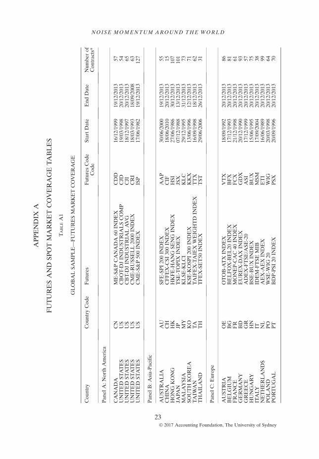
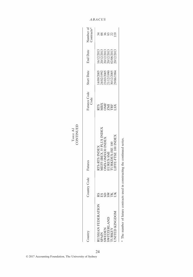
DataWe collect spot and futures data from 26 international markets to illustrate theexistence of noise momentum around the world. We use differential time periodscovering the complete lifespan of the daily index spot and futures contracts betweenJanuary 1982 (earliest available) and December 2013. The markets covered are:(a) North America—Canada and the US (four alternatives); (b) Asia-Pacific—Australia, China, Hong Kong, Japan, Malaysia, South Korea, and Thailand;(c) Europe—Austria, Belgium, France, Germany, Greece, Hungary, Netherlands,Poland, Portugal, Russian Federation, Spain, Switzerland, Turkey, and the UK.11

These markets are summarized in Appendix A, Table A1. Proxies for the risk-freeinterest rate are shown in Table A2. Divided yields on the indices are also collected.

10 In prior studies, transaction costs and market liquidity have been proposed to explain the temporarydeviation from the cost of carry model. Generally, it is documented that liquidity enhances the effi-ciency of the futures-cash pricing system (e.g., Stoll and Whaley, 1986; MacKinlay and Ramaswamy,1988; Roll et al., 2007). Temporary deviations from cost of carry also motivate several studies to em-ploy threshold error correction models (e.g., Yadav et al., 1994; Martens et al., 1995).

11 The power of our empirical tests is potentially weakened by the lower liquidity evident in some of theindividual markets included. While we clearly have a wide variation of liquidity across our sample, inunreported analysis, we find evidence of reasonable activity even in the emerging/developing marketsub-sample. Given that an illiquidity effect would tend to induce noise and make it harder to find thepredicted relationships, the fact that our results are uniformly strong allays any major concernsaround our research design in this regard.

ABACUS


The main data are sourced from DataStream and where the dividend yields and in-terest rate data are missing we supplement with data from Bloomberg. A continuousseries of the nearest term futures contracts is constructed by DataStream. The seriesswitch to the next nearest contract on the first day of the expiry month for thenearest term contract. We use a full set of expiry dates for all the contracts to ensurecorrect matching of the date to maturity in the continued futures price series.Table 1 reports the sample averages for all variables (measured in percentageterms), across the different markets in our full sample.As expected, the movements of the paired spot and futures prices closely mimic

each other. For each market, the average price changes are of the same magnitudewhile the volatilities are higher in the futures contracts. For example, in the case ofthe US S&P 500 (ISP), the average daily basis (the log difference between futuresand spot prices) is 0.36%. After applying the cost of carry model, the differencebetween the futures price and the fair estimate (f� f*) is, on average, zero.12 Similarfindings are documented in other country pairs. The mean pricing error is zero,suggesting that on average the markets are in equilibrium.

EMPIRICAL RESULTS

Initial Mispricing Correction around the World: One-period ECM ResultsThe detailed market-by-market estimation results for the one-period ECM inequation (12) are reported in Table 2, with an accompanying summary provided inTable 3. Our main focus in this baseline estimation is the role of the kappa param-eter, reflecting the initial mispricing correction. At a general level, we observe thatin all 29 cases the estimated coefficient is negative and significant (at the 1% level).Accordingly, there is pervasive evidence supporting the role of initial mispricingcorrection in futures-spot markets, in line with H1. That is, our analysis in thecontext of this simple ECM framework supports the view that arbitrageurs engagein initial mispricing correction (i.e., |κ| > 0). Moreover, we see the magnitude ofkappa estimates range in the (0,1) interval, thereby indicating that this initialcorrection phenomenon is consistent with limited arbitrage (i.e., |κ| < 1).Figure 1 plots the initial error correction parameters from highest to lowest

(in magnitude) across our sample of markets. We see that the maximum (minimum)magnitude of this effect occurs in Canada (Italy). Other large magnitude cases areevident for the US (except CJD), Japan, and Germany. These results suggest thata stronger role for initial mispricing correction is more likely to occur in the larger,more prominent markets. However, the patterns are quite mixed. While the devel-oping markets of China, Malaysia, and Poland exhibit small magnitude estimates,relatively close to zero, so too do the much bigger developed markets of Franceand the UK. Thus, while we do observe considerable variation across market

12 As expected, the point estimate of long-run coefficient θ across all markets is very close to (andstatistically indistinguishable from) unity. While full details of these analyses are suppressed hereto conserve space, they are available from the authors upon request.



TABLE 1

SAMPLE MEANS FOR BASE VARIABLES ACROSS MARKETS

Panel A: North America

Country CN US

Futures CDD CJD CJI CRI IS

Δf 4.14 3.66 4.08 7.21 8.32Δs 4.05 3.51 4.00 7.20 8.26f –s 0.05 0.03 0.06 0.044 0.36f –f* 0.00 0.00 0.00 0.00 0.00r 2.47 2.41 2.34 3.79 4.25q 2.00 2.24 2.24 1.19 2.50N 3710 4096 4211 4007 8242

Panel B: Asia-Pacific

Country AU CH HK JP KO MY TA THFutures AAP CIF HSI JSX KKX KLC TTX TST

Δf 3.79 �7.44 8.95 �2.00 5.03 3.19 0.40 7.14Δs 3.81 �7.56 8.86 �2.01 5.00 3.16 0.47 7.08f –s 0.09 0.38 0.10 0.14 0.19 0.06 �0.29 �0.50f –f* 0.00 0.00 0.00 0.00 0.00 0.00 0.00 0.00r 5.07 2.75 4.39 1.48 5.85 4.20 2.28 3.03q 3.99 1.57 3.30 0.78 2.53 0.66 2.99 3.87N 3539 942 7190 6581 4582 4682 4005 1977

Panel C: Europe

Country BD BG ES FR GR HN IT NLFutures GDX BFX MBX FCX ASI BUX MSM ETI

Δf 7.52 0.19 5.70 0.45 �13.34 13.00 �3.57 4.79Δs 7.48 0.27 5.64 0.41 �13.21 12.73 �3.27 4.77f –s 0.52 �0.04 �0.05 �0.05 �0.49 1.11 �0.35 0.01f –f* 0.00 0.03 0.00 0.00 0.00 0.00 0.00 0.00r 3.50 2.84 4.54 2.41 2.33 10.02 1.87 3.93q 1.98 3.33 3.51 3.36 3.17 1.63 1.85 3.47N 5846 4601 5636 3882 3716 4755 2526 6544

Country OE PO PT RS SD SW TK UKFutures VTX WIG PSX RTS OMF ZMI TRF LSX

Δf 1.24 3.60 �6.14 6.25 5.89 7.36 9.88 5.78Δs 0.18 3.85 �5.98 6.20 5.86 7.31 11.72 5.80f –s �0.29 �0.21 �0.23 �0.51 �0.14 �0.08 0.27 0.35f –f* 0.02 0.00 0.02 0.00 0.00 0.00 0.03 0.00r 2.59 8.08 2.63 4.38 1.72 2.27 11.76 7.10q 2.40 2.44 3.59 1.13 2.77 1.95 2.47 3.44N 3730 4137 3705 2169 2290 6012 1846 7713

This table reports the sample mean for all of the variables employed across each market. Table 6 in Ap-pendix A provides the full list of the markets covered. The variables included are: Δs (Δf) is the first dif-ference of log spot (futures) price; f �t;T ¼ st þ rt � qtð Þτt where st = ln (St), rt is the annualized risk-freeinterest rate on an investment for the period τt = T-t; qt is the annualized dividend yield on the index,while N is the sample size for each market. All numbers are tabulated in percentage point terms.

ABACUS


TABLE 2

ONE-PERIOD ECM ESTIMATION RESULTS—INITIAL MISPRICING CORRECTIONAROUND THE WORLD


Coeff. CN US

CDD CJD CJI CRI ISP

α 0.001 0.001 0.000 0.000 �0.002κ �0.714*** �0.039*** �0.617*** �0.558*** �0.394***ω �0.035*** �0.026*** �0.002 0.044*** 0.045***π �0.370*** �0.923*** �4.318 0.608*** 0.015N 3705 4091 4206 4002 8237


Coeff. AU CH 1HK JP KO MY 2TA THAAP CIF HSI JSX KKX KLC TTX TST

α 0.001 �0.002 0.002 0.000 0.001 0.000 0.001 0.000κ �0.301*** �0.151*** �0.268*** �0.512*** �0.162*** �0.102*** �0.180*** �0.235***ω �0.038*** �0.054*** �0.028*** 0.049*** 0.045*** 0.125*** 0.077*** 0.049***π �0.085 0.395** �1.077*** 1.006*** 1.932*** 0.984*** 0.992*** 0.998***N 3534 937 7185 6576 4577 4677 4000 1972

Panel C: Europe

Coeff. BD BG ES FR GR HN IT NLGDX BFX MBX FCX ASI BUX MSM ETI

α 0.001 0.005 0.017 0.000 �0.002 0.010 0.001 0.000κ �0.435*** �0.186*** �0.132*** �0.071*** �0.222*** �0.281*** �0.037*** �0.123***ω �0.019*** �0.029*** �0.727*** �0.020*** �0.027*** �0.139*** �0.035*** �0.008***π �0.435*** �0.423** 0.002 0.057 �1.059*** �0.330*** 0.808*** �0.616*N 5841 4464 5631 3877 3711 4750 2521 6539

Coeff. OE PO PT RS SD SW TK UKVTX WIG PSX RTS OMF ZMI TRF LSX

α 0.001 0.003 0.002 �0.001 0.001 0.001 0.039 0.001κ �0.148*** �0.051*** �0.082*** �0.228*** �0.094*** �0.137*** �0.193*** �0.098***ω �0.010* �0.059*** 0.006 0.076*** 0.012*** �0.007** �0.537*** 0.009***π �0.679 �0.722*** 3.584 0.959*** 3.891** �3.249** �0.162*** 3.062***N 3628 4132 3606 2164 2285 6007 1841 7708

This table reports the estimation results for the one-period ECM for pairs of futures contracts and countrystock indices, around the world, as listed in Table 6 in Appendix A. The ECM is specified as follows(equation (12)): Δf t ¼ αþ κzt�1 þ 1þ ωð ÞΔf �t þ �ωπð ÞΔf t�1 þ ut ;where Δ is the first difference operator;{α, κ,ω, π} are the parameters, and ut is the error term. The residual, zt ; of the long-run model is obtainedfrom the following estimation: f t ¼ μþ θf �t þ zt where ft is the natural log of the actual futures contractprice; f �t is the natural log of the fundamental value implied by the cost of carry model, f �t ¼ st þ rt � qtð Þτt;st is the natural log of the spot index price; rt is the risk-free rate; and qt is the dividend yield on the index.***, **, and * indicate significance at the 1%, 5%, and 10% levels, respectively.



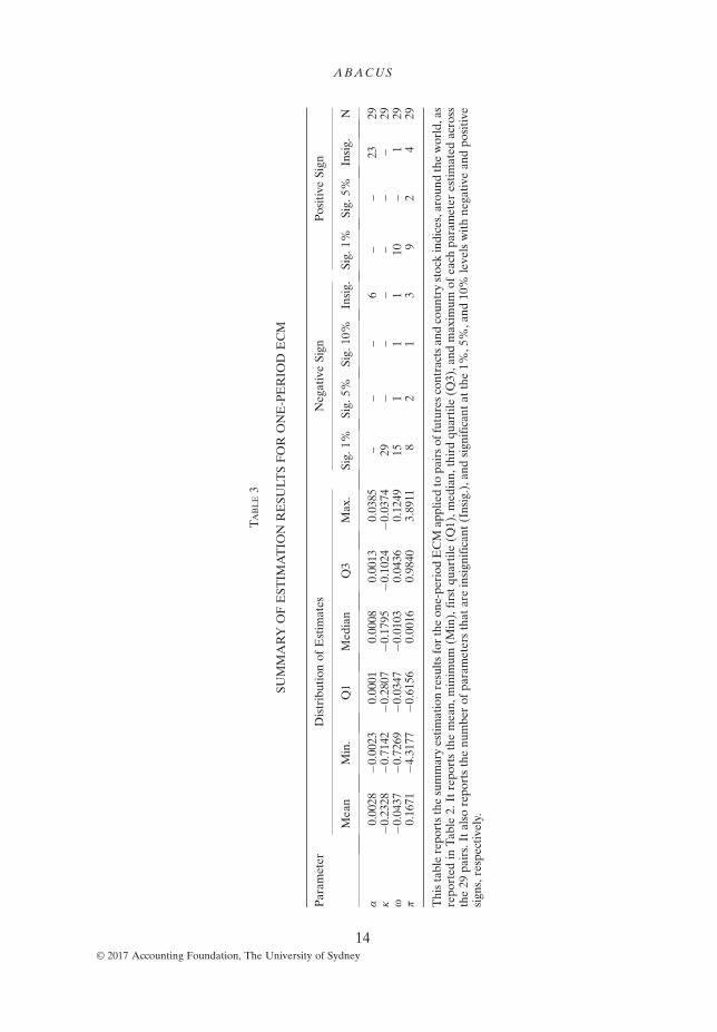
TABLE3

SUMMARY

OFEST

IMATIO

NRESU

LTSFOR

ONE-PERIO

DECM

Param

eter

Distributionof

Estim

ates

NegativeSign

PositiveSign

Mean

Min.

Q1

Med

ian

Q3

Max.

Sig.

1%Sig.

5%Sig.

10%

Insig.

Sig.

1%Sig.

5%Insig.

N

α0.0028

�0.0023

0.0001

0.0008

0.0013

0.0385

––

–6

––

2329

κ�0

.2328

�0.7142

�0.2807

�0.1795

�0.1024

�0.0374

29–

––

––

–29

ω�0

.0437

�0.7269

�0.0347

�0.0103

0.0436

0.1249

151

11

10–

129

π0.1671

�4.3177

�0.6156

0.0016

0.9840

3.8911

82

13

92

429

Thistablerepo

rtsthesummaryestimationresultsfortheon

e-pe

riod

ECM

appliedto

pairsof

futurescontractsan

dcoun

trystockindices,arou

ndtheworld,as

repo

rted

inTab

le2.

Itrepo

rtsthemean,

minim

um(M

in),firstqu

artile

(Q1),m

edian,

thirdqu

artile

(Q3),a

ndmaxim

umof

each

parameter

estimated

across

the29

pairs.Italso

repo

rtsthenu

mbe

rof

parametersthat

areinsign

ifican

t(Insig.),a

ndsign

ifican

tat

the1%

,5%,a

nd10%

levelswithne

gativ

ean

dpo

sitive

sign

s,respectively.

ABACUS


settings and we are unable to draw strong conclusions regarding any trends, we dopresent pervasive evidence of the predicted initial mispricing correction effect.

Noise Momentum around the World: Two-period GECM ResultsThe detailed market-by-market estimation results for the two-period GECM inequation (13) are reported in Table 4, with an accompanying summary provided inTable 5. In Table 4, various findings are worthy of special focus—primarily, thoselinking to our two key hypotheses. We see in the table that the estimated initialmispricing parameters, κ, are negative and significant in all 29 cases, once moremimicking the outcome of the one-period ECM. Again, this supports the limits toarbitrage version of the initial mispricing correction hypothesis (H1).Based on the range of point estimates produced, the median value (with a

magnitude of approximately 41%) suggests that just under half of the prior periodpricing error is corrected. It is noteworthy that this is a much higher correction thanthe counterpart median observed in the one-period ECM—with a value less than20% in magnitude. Indeed, comparing the initial mispricing correction coefficientsbetween the ECM and GECM models market-by-market, in most cases it appearsthat arbitrageurs play a much bigger role in bringing the price back to its fundamen-tal value than suggested by the simpler ECM setup. Only in the case of Spain doesthe magnitude of the estimate not increase. Such a contrasting result suggests thatthe one-period ECM gives a biased and unreliable view of the initial errorcorrection forces evident in the data. This is most noticeable for the French and

FIGURE 1

INITIAL MISPRICING CORRECTION IMPLIED BY THE ONE-PERIOD ECM

[Color figure can be viewed at wileyonlinelibrary.com]



TABLE 4

TWO-PERIOD GECM ESTIMATION RESULTS—NOISEMOMENTUMAROUND THEWORLD


Coeff. CN US

CDD CJD CJI CRI ISP

α 0.001 0.000 0.000 �0.001 �0.002κ �0.761*** �0.188*** �0.705*** �0.652*** �0.540***λ 0.694*** 0.190*** 0.752*** 0.523*** 0.466***ω �0.033*** �0.023*** 0.000 0.047*** 0.048***π �0.199 �0.573** 19.672 0.300*** �0.390***N 3705 4091 4206 4002 8237


Coeff. AU CH HK JP KO MY TA THAAP CIF HSI JSX KKX KLC TTX TST

α 0.001 �0.001 0.000 0.001 0.000 �0.001 0.001 �0.001κ �0.518*** �0.365*** �0.410*** �0.629*** �0.349*** �0.325*** �0.365*** �0.462***λ 0.636*** 0.399*** 0.316*** 0.572*** 0.328*** 0.343*** 0.342*** 0.524***ω �0.033*** �0.052*** �0.020*** 0.051*** 0.050*** 0.125*** 0.079*** 0.053***π 0.467*** 0.492*** �0.103 0.540*** 0.998*** 0.401*** 0.563*** 0.259*N 3534 937 7185 6576 4577 4677 4000 1972

Panel C: Europe

Coeff. BD BG ES FR GR HN IT NLGDX BFX MBX FCX ASI BUX MSM ETI

α 0.001 0.004 0.016 0.000 0.000 0.007 0.002 0.000κ �0.599*** �0.462*** �0.101*** �0.324*** �0.474*** �0.454*** �0.197*** �0.404***λ 0.725*** 0.610*** �0.088*** 0.404*** 0.602*** 0.436*** 0.206*** 0.536***ω �0.016*** �0.032*** �0.707*** �0.020*** �0.030*** �0.138*** �0.034*** �0.008***π �0.115 0.363** �0.001 0.204* 0.357 0.004 0.858*** 0.514N 5841 4464 5631 3877 3711 4750 2521 6539

Coeff. OE PO PT RS SD SW TK UKVTX WIG PSX RTS OMF ZMI TRF LSX

α �0.002 0.003 0.003 �0.002 0.000 0.001 0.033 0.000κ �0.450*** �0.188*** �0.364*** �0.415*** �0.357*** �0.447*** �0.431*** �0.349***λ 0.636*** 0.178*** 0.475*** 0.395*** 0.450*** 0.648*** 0.494*** 0.423***ω �0.009 �0.055*** 0.005 0.082*** 0.015*** �0.006** �0.547*** 0.014***π 3.207 �0.563*** -2.982 0.435*** 1.862*** �1.613** 0.171*** 0.555**N 3628 4132 3606 2164 2285 6007 1841 7708

This table reports the estimation results of the two-period GECM for pairs of futures contracts and coun-try stock indices, around the world, as listed in Table 6 in Appendix A. The GECM is specified as follows(equation (13)):Δf t ¼ αþ κzt�1 þ λ 1þ κð Þzt�2 þ 1þ ωð ÞΔf �t þ �ωπð ÞΔf t�1 þ ut where Δ is the first differ-ence operator; {α, κ, λ,ω, π} are the parameters, and ut is the error term. The residual, zt; of the long-runmodel is obtained from the following estimation: f t ¼ μþ θf �t þ zt where ft is the natural log of the actualfutures contract price; f �t is the natural log of the fundamental value implied by the cost of carry model,f �t ¼ st þ rt � qtð Þτt; st is the natural log of the spot index price; rt is the risk-free rate; and qt is the dividendyield on the index. ***, **, and * indicate significance at the 1%, 5%, and 10% levels, respectively.

ABACUS


TABLE5

SUMMARY

OFEST

IMATIO

NRESU

LTSFOR

TWO-PERIO

DGECM

Param

eter

Distributionof

Estim

ates

Neg

ativeSign

PositiveSign

Mea

nMin.

Q1

Med

ian

Q3

Max

.Sig.

1%Sig.

5%Sig.

10%

Insig.

Sig.

1%Sig.

5%Sig.

10%

Insig.

N

α0.00

22�0

.002

3�0

.000

30.00

030.00

100.03

31–

––

10–

––

1929

κ�0

.423

6�0

.761

4�0

.474

0�0

.414

8�0

.349

3�0

.100

929

––

––

––

–29

λ0.45

56�0

.088

20.34

320.46

620.60

230.75

211

––

–28

––

–29

ω�0

.0411

�0.707

1�0

.033

1�0

.008

80.04

660.12

5415

1–

110

––

229

π0.88

56�2

.982

0�0

.103

10.35

710.53

9619

.672

32

2–

511

22

529

Thistablerepo

rtsthesummaryestimationresultsforthetw

o-pe

riod

GECM

appliedto

pairsof

futurescontractsan

dcoun

trystockindices,arou

ndtheworld,

asrepo

rted

inTab

le4.Itrepo

rtsthemean,

minim

um(M

in),firstq

uartile

(Q1),m

edian,

thirdqu

artile(Q

3),and

maxim

umof

each

parameter

estimated

across

the29

pairs.Italso

repo

rtsthenu

mbe

rof

parametersthat

areinsign

ifican

t(Insig.),a

ndsign

ifican

tat

the1%

,5%,a

nd10%

levelswithne

gative

andpo

sitive

sign

s,respectively.



UK markets—while both of these in the ECM analysis showed statistically signifi-cant correction effects, neither seemed to differ markedly from zero in economicterms. Now both France and the UK show coefficient estimates exceeding 30%,which is much more economically meaningful.Our primary focus is on the estimated noise momentum coefficient (λ), which

links to the ‘noise momentum’ hypothesis, H2. Notably, in Tables 4 and 5 we findthat the effect of noise momentum is positive and significant in all but one case(the one exception is Spain). This finding provides strong support for our noisemomentum hypothesis which highlights that, over and above any correction for ini-tial mispricing in the first period, the convergence to equilibrium displays a degreeof momentum in the mispricing or ‘noise’ component. It is noteworthy that all theestimated positive coefficients are less than unity.Looking at the country-by-country results, we see the overall maximum case of

noise momentum occurs in the US market (CJI) with a value of 0.752, closelyshadowed by Canada (0.694). In the Asia-Pacific region, Australia (0.637) andJapan (0.572) produce the highest values, while in Europe, Germany (0.725) andSweden (0.649) are prominent. At the other end of the spectrum, aside fromSpain, which exhibits the only negative noise momentum coefficient, we have Italy(0.206) and Poland (0.178) standing out with the lowest values. Nevertheless, nostrong patterns emerge, for example, in terms of a developed versus emergingmarket divide. For a visual appreciation, Figure 2 plots the Kappa and Lambdaparameters produced by the GECM across our sample of markets.For completeness, we make some closing general observations regarding the

remaining estimated parameters of the two-period model. First, regarding the inter-cept we see that in all cases it is insignificant. While not a guarantee, it is suggestivethat the specification is one not greatly challenged by mis-specification. In otherwords, the empirical specification is closely matched with the theoretical model inwhich this parameter is expected to be zero.Second, regarding the parameter ω, we observe only three instances of insignifi-

cance—we have 16 (10) significant negative (positive) cases, at the 10% level or bet-ter. Recall that in the context of equation (10), which decomposes the pricing errorsinto its various parts, the ω coefficient relates to the component that measures thedegree of the over- or underreaction with respect to the contemporaneous funda-mental changes. Our findings suggest that the futures price is more likely to under-react than overreact on the fundamentals shocks from the underlying stock index.Finally, regarding parameter π, there is a preponderance of (few) significant cases with

a positive (negative) sign, namely, 15 (four) cases at the 10% level. Recall that in thecontext of equation (4), this coefficient relates to the short-run momentum effect.Specifically, a positive (negative) π implies positive (negative) feedback trading. Ac-cordingly, this GECM analysis suggests a high incidence of positive feedback trading.

Speed of Mispricing Correction and Duration of Error ConvergenceAs indicated earlier, measuring the speed of mispricing correction is a point ofcontrast between our two models: in the one-period ECM it is given by κ, whereasin the two-period GECM it is a function of both initial mispricing correction, κ,

ABACUS


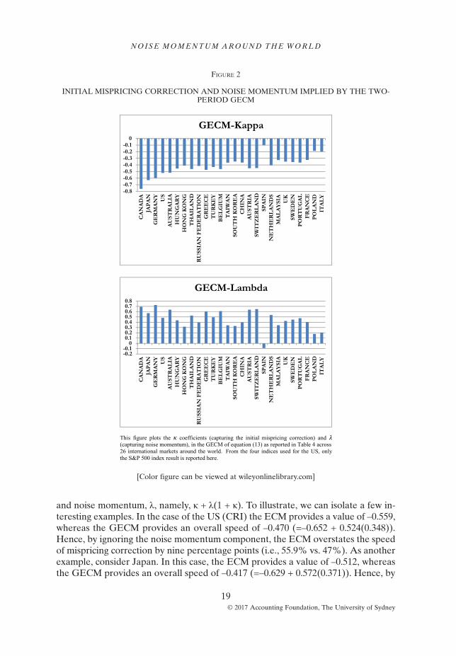
and noise momentum, λ, namely, κ + λ(1 + κ). To illustrate, we can isolate a few in-teresting examples. In the case of the US (CRI) the ECM provides a value of –0.559,whereas the GECM provides an overall speed of –0.470 (=–0.652 + 0.524(0.348)).Hence, by ignoring the noise momentum component, the ECM overstates the speedof mispricing correction by nine percentage points (i.e., 55.9% vs. 47%). As anotherexample, consider Japan. In this case, the ECM provides a value of –0.512, whereasthe GECM provides an overall speed of –0.417 (=–0.629 + 0.572(0.371)). Hence, by

FIGURE 2

INITIAL MISPRICING CORRECTION AND NOISE MOMENTUM IMPLIED BY THE TWO-PERIOD GECM




ignoring the noise momentum component, the ECM overstates the speed ofmispricing correction by close to 10 percentage points (i.e., 51% vs. 41%). As a finalexample, consider Italy. In this case, the ECM provides a value of –0.037, whereasthe GECM provides an overall speed of –0.0316 (=–0.197 + 0.206(0.803)).An associated question of interest is how long does it take the price change to con-

verge to its long-run value, implied by either of our models? In other words, what isthe ‘duration’ (in days) of the mispricing error convergence? The answer to thisquestion is quite simply evaluated by taking the reciprocal of the (overall) adjust-ment coefficient. To this end, Figure 3 provides a comparative plot of the error du-ration implied by the ECM versus GECM models.Generally, it is true that we see somewhat similar values in several cases, but this

belies the relative role of the underlying components (i.e., Kappa versus Lambda),as discussed above. Consider a few interesting examples. At the short end of the spec-trum, across our sample markets, the US (CRI) exhibits durations of 1.8 days versus2.1 days for the ECM versus GECMmodels. In contrast, for the longest durations wesee Italy with values of 27 days versus 31.6 days for the ECM versus GECM models.Thus, regarding the question of the duration of error convergence, while it seems tomatter little for the US, the choice of modelling ECM versus GECM does make anappreciable difference for a market like Italy. Nevertheless, in percentage terms wegenerally see a nontrivial difference between the alternative paired duration esti-mates—in the order of 15% (measured relative to the ECM benchmark).

FIGURE 3

DURATION OF MISPRICING IN ECM AND GECM MODELS


ABACUS


CONCLUSION

Building on Shleifer and Vishny’s (1997) theoretical work, we study the dynamics oflimited arbitrage. Shleifer and Vishny’s (1997) model shows an important insightinto why arbitrageurs might deliberately limit their initial arbitrage, given their con-cern about further mispricing in the next period. We show that second-period errorpersistence (labelled ‘noise momentum’) is an important parameter in characteriz-ing the overall speed of the adjustment process, augmenting the initial error correc-tion coefficient as commonly used in the standard one-period ECM.To test our model predictions, we develop a two-period error correction model.

We apply our model to study the dynamics of limited arbitrage in the index futuresmarket, an important area of ongoing research interest in its own right. Using paireddaily index futures and spot data from 26 international markets over the maximumperiod 1984–2012, in addition to initial mispricing error we document pervasiveevidence of limited arbitrage linked to noise momentum around the world.Notably, the significance of this noise momentum coefficient suggests a serious

misspecification in the standard error correction models used in the literature.Our empirical application illustrates that the generalized error correction modelwe develop for the purpose provides a powerful tool for analyzing the dynamicsof the price–fundamentals relationship. The potential applications of this approachgo well beyond that developed in the current paper. For example, our approachcan be applied to explore the short-term dynamics associated with fundamentallong-run cointegrating relationships (e.g., the price–dividend relationship) and thepricing dynamics between segmented markets for single assets (e.g., cross-listingand commodity contracts in different markets). We commend these and other mean-ingful applications to future research agendas.

REFERENCES

Abreu, D. and M. K. Brunnermeier (2002), ‘Synchronization Risk and Delayed Arbitrage’, Journal of Fi-nancial Economics, Vol. 66, Nos 2–3, pp. 341–60.

—— (2003), ‘Bubbles and Crashes’, Econometrica, Vol. 71, No. 1, pp. 173–204.

Brenner, R. J. and K. F. Kroner (1995), ‘Arbitrage, Cointegration, and Testing the Unbiasedness Hypoth-esis in Financial Markets’, Journal of Financial and Quantitative Analysis, Vol. 30, No. 1, pp. 23–42.

Buraschi, A., M. Menguturk, and E. Sener (2014), ‘The Geography of Funding Markets and Limits to Ar-bitrage’, Review of Financial Studies, Vol. 28, No. 4, pp. 1103–52.

Chan, K. (1992), ‘A Further Analysis of the Lead–Lag Relationship between the Cash Market and StockIndex Futures Markets’, Review of Financial Studies, Vol. 5, No. 1, pp. 123–52.

DeLong, J. B., A. Shleifer, L. H. Summers, and R. J. Waldmann (1990a), ‘Noise Trader Risk in FinancialMarkets’, Journal of Political Economy, Vol. 98, No. 4, pp. 703–38.

—— (1990b), ‘Positive Feedback Investment Strategies and Destabilizing Rational Speculation’, Journalof Finance, Vol. 45, No. 2, pp. 379–95.

Edmans, A., I. Goldstein, and W. Jiang (2014), Feedback Effects and the Limits to Arbitrage, UnpublishedManuscript, London Business School, London.

Garbade, K. D. and W. L. Silber (1983), ‘Price Movements and Price Discovery in Futures and CashMarkets’, Review of Economics and Statistics, Vol. 65, No. 2, pp. 289–97.



Ghosh, A. (1993), ‘Cointegration and Error Correction Models: Intertemporal Causality between Indexand Futures Prices’, Journal of Futures Markets, Vol. 13, No. 7, pp. 193–98.

Gromb, D. and D. Vayanos (2010), ‘Limits of Arbitrage: The State of the Theory’, 8 March, available atSSRN: http://ssrn.com/abstract=1567243, accessed 26 June 2014.

Hasbrouck, J. (1991), ‘Measuring the Information Content of Stock Trades’, Journal of Finance, Vol. 46,No. 1, pp. 179–207.

Hombert, J. and D. Thesmar (2009), ‘Limits of Limits of Arbitrage: Theory and Evidence’, 5 March,available at SSRN: http://ssrn.com/abstract=1352285, accessed 26 June 2014.

Hull, J. C. (2008), Fundamentals of Futures and Options Markets, 6th edition, Prentice Hall, New Jersey.

Kondor, P. (2004), ‘Rational Trader Risk’, Discussion Paper, 533, Financial Markets Group, LondonSchool of Economics and Political Science, London, available at: http://eprints.lse.ac.uk/24646/,accessed 26 June 2014.

—— (2009), ‘Risk in Dynamic Arbitrage: Price Effects of Convergence Trading’, Journal of Finance,Vol. 64, pp. 638–58.

Kurov, A. and D. Lasser (2004), ‘Price Dynamics in the Regular and E-Mini Futures Market’, Journal ofFinancial and Quantitative Analysis, Vol. 39, No. 2, pp. 365–84.

Liu, J. and F. A. Longstaff (2004), ‘Losing Money on Arbitrages: Optimal Dynamic PortfolioChoice in Markets with Arbitrage Opportunities’, Review of Financial Studies, Vol. 17, No.3, pp. 611–41.

Ljungqvist A. and W. Qian (2014), How Binding Are Limits to Arbitrage?, Unpublished Manuscript,Stern School of Business, New York University, New York.

MacKinlay, A. C. and K. Ramaswamy (1988), ‘Index-futures Arbitrage and the Behavior of Stock IndexFutures Prices’, Review of Financial Studies, Vol. 1, pp. 137–58.

Makarov, I. and G. Plantiny (2012), Deliberate Limits to Arbitrage, Unpublished Manuscript, LondonBusiness School, London.

Martens, M., P. Kofman, and T. C. F. Vorst (1995), ‘A Threshold Error Correction Model for IntradayFutures and Index Returns’, Journal of Applied Econometrics, Vol. 13, No. 3, pp. 245–63.

Moreira, A. (2012), Limits to Arbitrage and Lockup Contracts, Unpublished Manuscript, Yale School ofManagement.

Oehmke, M. (2009), ‘Gradual Arbitrage’, 16 December, available at SSRN: http://ssrn.com/ab-stract=1364126, accessed 26 June 2014.

Panos, A. M., R. Nobay, and D. A. Peel (1997), ‘Transactions Costs and Nonlinear Adjustment in RealExchange Rates: An Empirical Investigation’, Journal of Political Economy, Vol. 105, pp. 862–79.

Roll, R., E. Schwartz, and A. Subrahmanyam (2007), ‘Liquidity and the Law of One Price: The Case ofthe Futures/Cash Basis’, Journal of Finance, Vol. 62, No. 5, pp. 2201–34.

Sercu, P., R. Uppal, and C. V. Hulle (1995), ‘The Exchange Rate in the Presence of Transaction Costs:Implications for Tests of Purchasing Power Parity’, Journal of Finance, Vol. 50, No. 4, pp. 1309–19.

Shleifer, A. and R. W. Vishny (1997), ‘The Limits of Arbitrage’, Journal of Finance, Vol. 52, No. 1,pp. 35–55.

Stein, J. C. (2009), ‘Presidential Address: Sophisticated Investors and Market Efficiency’, Journal ofFinance, Vol. 64, No. 4, pp. 1517–48.

Stoll, H. R. and R. E. Whaley (1986), Expiration Day Effects of Index Options and Futures, MonographSeries in Finance and Economics, Monograph 1986-3.

—— (1990), ‘The Dynamics of Stock Index and Stock Index Futures Returns’, Journal of Financial andQuantitative Analysis, Vol. 25, No. 4, pp. 441–68.

Wahab, M. and M. Lashgari (1993), ‘Price Dynamics and Error Correction in Stock Index and Stock In-dex Futures Markets: A Cointegration Approach’, Journal of Futures Markets, Vol. 13, pp. 711–42.

Yadav, P. K., P. F. Pope, and K. Paudyal (1994), ‘Threshold Autoregressive Modeling in Finance: ThePrice Differences of Equivalent Assets’, Mathematical Finance, Vol. 4, No. 2, pp. 205–21.

ABACUS


http://ssrn.com/abstract=1567243


http://eprints.lse.ac.uk/24646/



ATABLEA1

GLOBALSA

MPLE—FUTURESMARKETCOVERAGE

Cou

ntry

Cou

ntry

Cod

eFutures

Futures

Cod

eCod

eStartDate

End

Date

Num

berof

Con

tracts*

Pan

elA:N

orth

America

CANADA

CN

ME-S&PCANADA

60IN

DEX

CDD

16/12/1999

19/12/2013

57UNIT

ED

STATES

US

CBOT-DJIN

DUST

RIA

LSCOMP

CJD

19/03/1998

20/12/2013

54UNIT

ED

STATES

US

CBT-DJIN

DUST

RIA

LAVG

CJI

18/12/1997

20/12/2013

65UNIT

ED

STATES

US

CME-R

USS

ELL2000

INDEX

CRI

18/03/1993

18/09/2008

63UNIT

ED

STATES

US

CME-S&P500IN

DEX

ISP

17/06/1982

19/12/2013

127

Pan

elB:A

sia-Pacific

AUST

RALIA

AU

SFE-SPI200IN

DEX

AAP

30/06/2000

19/12/2013

55CHIN

ACH

CFFEX-C

SI300IN

DEX

CIF

18/06/2010

20/12/2013

15HONG

KONG

HK

HKFE-H

ANG

SENG

INDEX

HSI

27/06/1986

30/12/2013

107

JAPA

NJP

TSE

-TOPIX

INDEX

JSX

07/12/1988

13/12/2013

101

MALAYSIA

MY

KLSE

-KLCI

KLC

29/12/1995

31/12/2013

73SO

UTH

KOREA

KO

KSE

-KOSP

I200IN

DEX

KKX

13/06/1996

12/12/2013

71TAIW

AN

TA

TAIFEX-TAIE

XWEIG

HTD

INDEX

TTX

16/09/1998

18/12/2013

62THAIL

AND

TH

TFEX-SET50

INDEX

TST

29/06/2006

26/12/2013

31

Pan

elC:E

urop

e

AUST

RIA

OE

OTOB-A

TX

INDEX

VTX

18/09/1992

20/12/2013

86BELGIU

MBG

BELFOX-B

EL20

INDEX

BFX

17/12/1993

20/12/2013

81FRANCE

FR

MONEP-C

AC

40IN

DEX

FCX

21/12/1998

20/12/2013

61GERMANY

BD

EUREX-D

AX

INDEX

GDX

20/12/1990

20/12/2013

93GREECE

GR

ADEX-FTSE

/ASE

-20

ASI

17/12/1999

20/12/2013

57HUNGARY

HN

BSE

-BUX

INDEX

BUX

15/06/1995

20/12/2013

75ITALY

ITID

EM-FTSE

MIB

MSM

17/09/2004

20/12/2013

38NETHERLANDS

NL

AEX-A

EX

INDEX

ETI

16/06/1989

20/12/2013

99POLAND

PO

WSE

-WIG

20WIG

20/03/1998

20/12/2013

64PORTUGAL

PT

BDP-PSI

20IN

DEX

PSX

20/09/1996

20/12/2013

70

APPENDIX

A

FUTURESAND

SPOTMARKETCOVERAGE

TABLES



TABLEA1

CONTIN

UED

Cou

ntry

Cou

ntry

Cod

eFutures

Futures

Cod

eCod

eStartDate

End

Date

Num

berof

Con

tracts*

RUSS

IAN

FEDERATIO

NRS

RTS-RTSIN

DEX

RTS

14/09/2005

16/12/2013

34SP

AIN

ES

MEFF-IBEX

35PLUSIN

DEX

MBX

24/02/1992

20/12/2013

88SW

EDEN

SDOMX-O

MXS3

0IN

DEX

OMF

23/03/2005

20/12/2013

36SW

ITZERLAND

SWEUREX-SMI

ZMI

21/12/1990

20/12/2013

93TURKEY

TK

TURKDEX-ISE

100

TRF

30/12/2005

02/08/2013

22UNIT

ED

KIN

GDOM

UK

LIFFE-FTSE

100IN

DEX

LSX

29/06/1984

20/12/2013

119

*The

numbe

rof

future

contractsused

inconstructing

thecontinue

dseries.

ABACUS


TABLEA2

GLOBALSA

MPLE—UNDERLY

ING

STOCK

INDEX

COVERAGE

Cou

ntry

Cou

ntry

Cod

eUnd

erlin

gInde

xInterest

Rate

Currency

Pan

elA:N

orth

America

CANADA

CN

S&P/TSX

60IN

DEX

CANADA

TREASU

RY

BIL

L3MONTH

(BOC)

C$

UNIT

ED

STATES

US

DOW

JONESIN

DUST

RIA

LS

UST-BIL

LSE

CMARKET3MONTH

(D)

U$

UNIT

ED

STATES

US

DOW

JONESIN

DUST

RIA

LS

UST-BIL

LSE

CMARKET3MONTH

(D)

U$

UNIT

ED

STATES

US

RUSS

ELL2000

UST-BIL

LSE

CMARKET3MONTH

(D)

U$

UNIT

ED

STATES

US

S&P500COMPOSITE

UST-BIL

LSE

CMARKET3MONTH

(D)

U$

Pan

elB:A

sia-Pacific

AUST

RALIA

AU

S&P/A

SX200

AUST

RALIA

N$DEPO

3MONTH

(ICAP/TR)Rate

A$

CHIN

ACH

CHIN

ASE

CURIT

IES300

CHIN

AREPO

3MONTH

CH

HONG

KONG

HK

HANG

SENG

TR

HONG

KONG

DOLLAR

3M

DEPOSIT

K$

JAPA

NJP

TOPIX

JPCD

RATESFIN

INS30–59D,A

VG

YMALAYSIA

MY

FTSE

BURSA

MALAYSIA

KLCI

MALAYSIA

INTERBANK

3MONTH

M$

SOUTH

KOREA

KO

KOREA

SEKOSP

I200

KOREA

NCD

91DAYS

KW

TAIW

AN

TA

TAIW

AN

SEWEIG

HED

TAIE

XTAIW

AN

MONEY

MARKET90

DAYS

TW

THAIL

AND

TH

BANGKOK

S.E.T.5

0BANGKOK

INTERBANK

3MONTH

TB

Pan

elC:E

urop

e

AUST

RIA

OE

ATX:A

UST

RIA

NTRADED

INDEX

BrusselsInterban

kOffered

Rate

EBELGIU

MBG

BEL20

BD

EU-M

ARK

3M

DEPOSIT(FT/TR)

EFRANCE

FR

FRANCE

CAC

40EURO

SHORTTERM

REPO

(ECB)

EGERMANY

BD

DAX

30PERFORMANCE

(XETRA)

EURO

SHORTTERM

REPO

(ECB)

EGREECE

GR

FTSE

/ATHEX

LARGE

CAP

EURO

SHORTTERM

REPO

(ECB)

EHUNGARY

HN

BUDAPEST

(BUX)

HUNGARY

INTERBANK

3MONTH

HF

ITALY

ITFTSE

MIB

INDEX

EURO

SHORTTERM

REPO

(ECB)

ENETHERLANDS

NL

AEX

INDEX

(AEX)

NETHERLAND

INTERBANK

3MONTH

EPOLAND

PO

WARSA

WGENERALIN

DEX

20WARSA

WIN

TERBANK

3MONTH

PZ

PORTUGAL

PT

PORTUGALPSI-20

OECD

PortugalInterestRates

3Mon

thVIB

OR

E



TABLEA2

CONTIN

UED

Cou

ntry

Cou

ntry

Cod

eUnd

erlin

gInde

xInterest

Rate

Currency

RUSS

IAN

FEDERATIO

NRS

RUSS

IARTSIN

DEX

RUSS

IAIN

TERBANK

31TO

90DAY

U$

SPAIN

ES

IBEX

35SP

AIN

INTERBANK

W/A

3M

(DISC)

ESW

EDEN

SDOMX

STOCKHOLM

30(O

MXS3

0)SW

EDEN

TREASU

RY

BIL

L90

DAY

SKSW

ITZERLAND

SWSW

ISSMARKET(SMI)

SWISS3MONTH

LIB

OR

(SNB)

SFTURKEY

TK

BISTNATIO

NAL100

TURKISH

INTERBANK

3MONTH

TL

UNIT

ED

KIN

GDOM

UK

FTSE

100

UK

INTERBANK

3MONTH

£

ABACUS


Noise Momentum Around the World - UQ eSpace

Documents

Transcript of Noise Momentum Around the World - UQ eSpace