Noise-invariant Neurons in the Avian Auditory Cortex: Hearing the Song in Noise

Noise-invariant Neurons in the Avian Auditory Cortex:Hearing the Song in NoiseR. Channing Moore1, Tyler Lee2, Frederic E. Theunissen1,2,3*

1 Biophysics Graduate Group, University of California, Berkeley, Berkeley, California, United States of America, 2 Helen Wills Neuroscience Institute, University of California,

Berkeley, Berkeley, California, United States of America, 3 Department of Psychology, University of California, Berkeley, Berkeley, California, United States of America

Abstract

Given the extraordinary ability of humans and animals to recognize communication signals over a background of noise,describing noise invariant neural responses is critical not only to pinpoint the brain regions that are mediating our robustperceptions but also to understand the neural computations that are performing these tasks and the underlying circuitry.Although invariant neural responses, such as rotation-invariant face cells, are well described in the visual system, high-levelauditory neurons that can represent the same behaviorally relevant signal in a range of listening conditions have yet to bediscovered. Here we found neurons in a secondary area of the avian auditory cortex that exhibit noise-invariant responses inthe sense that they responded with similar spike patterns to song stimuli presented in silence and over a background ofnaturalistic noise. By characterizing the neurons’ tuning in terms of their responses to modulations in the temporal andspectral envelope of the sound, we then show that noise invariance is partly achieved by selectively responding to longsounds with sharp spectral structure. Finally, to demonstrate that such computations could explain noise invariance, wedesigned a biologically inspired noise-filtering algorithm that can be used to separate song or speech from noise. This novelnoise-filtering method performs as well as other state-of-the-art de-noising algorithms and could be used in clinical orconsumer oriented applications. Our biologically inspired model also shows how high-level noise-invariant responses couldbe created from neural responses typically found in primary auditory cortex.

Citation: Moore RC, Lee T, Theunissen FE (2013) Noise-invariant Neurons in the Avian Auditory Cortex: Hearing the Song in Noise. PLoS Comput Biol 9(3):e1002942. doi:10.1371/journal.pcbi.1002942

Editor: Konrad P. Kording, Northwestern University, United States of America

Received January 4, 2012; Accepted January 10, 2013; Published March 7, 2013

Copyright: � 2013 Moore et al. This is an open-access article distributed under the terms of the Creative Commons Attribution License, which permitsunrestricted use, distribution, and reproduction in any medium, provided the original author and source are credited.

Funding: The work was funded by NIDCD 010132 grant to FET. The funders had no role in study design, data collection and analysis, decision to publish, orpreparation of the manuscript.

Competing Interests: The authors have declared that no competing interests exist.

* E-mail: [email protected]

Introduction

Invariant neural representations of behaviorally relevant objects

are a hallmark of high-level sensory regions and are interpreted as

the outcome of a series of computations that would allow us to

recognize and categorize objects in real life situations. For example,

view-invariant face neurons have been found in the inferior

temporal cortex [1] and are thought to reflect our abilities to

recognize the same face from different orientations and scales. The

representation of auditory objects by the auditory system is less

well understood although neurons in high-level auditory areas can

be very selective for complex sounds and, in particular,

communication signals[2]. It has also been shown that auditory

neurons can be sound level invariant [3,4] or pitch sensitive [5]. As

is the case for all neurons labeled as invariant, pitch sensitive

neurons respond similarly to many different stimuli as long as these

sounds yield the same pitch percept. Both sound level invariant

and pitch sensitive neurons could therefore be building blocks in

the computations required to produce invariant responses to

particular auditory signals subject to distortions due to propaga-

tions or corruption by other auditory signals. The existence of such

distortion invariant auditory neurons, however, remains unknown.

Similarly, the neuronal computations required to recognize

communication signals embedded in noise are not well understood

although it is known that humans [6] and other animals [7] excel

at this task.

In this study, we examined how neurons in the secondary avian

auditory cortical area NCM (CaudoMedial Nidopalium) responded to

song signals embedded in background noise to test whether this

region presents noise-invariant characteristics that could be

involved in robust song recognition. We chose the avian model

system because birds excel at recognizing individuals based on

their communication calls [8], often in very difficult situations [9].

Moreover, the avian auditory system is well characterized and it is

known that neurons in higher-level auditory regions can respond

selectively to particular conspecific songs [10]. We focused our

study on NCM because a series of neurophysiological [11,12] and

immediate early gene studies [13,14] have implicated this

secondary auditory area in the recognition of familiar songs. In

addition, although neuronal responses in the primary avian

auditory cortex regions are systematically degraded by noise

[15], studies using immediate early gene activation suggested that

responses to conspecific song in NCM were relatively constant for

a range of behaviorally relevant noise levels [16].

Results/Discussion

We recorded neural responses from single neurons in NCM of

anesthetized adult male Zebra Finches. We obtained responses to

40 different unfamiliar conspecific songs and to the same songs

embedded in naturalistic synthetic noise also called modulation-

limited noise (ml-noise from here on). Ml-noise is broadband

PLOS Computational Biology | www.ploscompbiol.org 1 March 2013 | Volume 9 | Issue 3 | e1002942

white-noise that has been filtered in the modulation domain to

mimic the structure that is found in environmental sounds by

restricting the power of modulations in the envelope to low

spectral-temporal frequencies [17]. Ml-noise has also been shown

to be an efficient stimulus for driving high-level auditory neurons

(see Methods for additional details). The signal to noise ratio

(SNR) was set at 3dB.

Noise Invariant Neurons in NCMAs illustrated on the left panels in Fig. 1, responses of some

neurons to song signal were almost completely masked by the

addition of noise. In these situations, the post-stimulus time

histogram (PSTH) obtained for song only (third row) is very

different than the one obtained for song + ml-noise (fifth row).

However, some neurons also showed strong robustness to noise

degradation as illustrated on the right panels of Fig. 1. Those

neurons had similar PSTHs for both conditions.

To quantify the degree of noise robustness, we calculated two

measures of noise-invariance: a de-biased correlation coefficient

between the PSTHs obtained for the song alone and song + ml-

noise stimuli (called ICC) and the ratio of the SNR estimated for

the song + noise response and the song + ml-noise response (ISNR

invariance). The ICC metric is a normalized measure that ranges in

values between 21 and 1. It is 1 when the response pattern

observed to song+ml-noise is identical to the one observed to song,

irrespective of the relative magnitude of the two responses. For

ISNR, we defined the response SNR as follows. For the response to

song alone, the signal power was defined as the variance in the

PSTH across time and the noise was defined as the mean firing

rate. For the response to song plus noise, the signal was taken to be

the time-varying response that could be predicted linearly from the

response to song alone and the noise was the mean of this

predicted response (see methods). This second value of invariance

is bounded between 0 and 1 and captures not only the similarities

in response patterns but also magnitudes of time-varying responses

that carry information about the song. As shown in the

supplemental material, the two measures were highly correlated

and subsequent analyses resulted in very similar results and

identical conclusions. For brevity, we show the analysis using the

ICC metric in the main paper. Some of the results with the ISNR

metric are included in the supplemental material.

Noise Invariance and Frequency TuningWe found neurons with different degrees of noise invariance

throughout NCM but the neurons in the ventral region tended to

have highest Icc (Fig. 2B). NCM also exhibits some degree of

frequency tonotopy along this dimension with higher frequency

tuning found in more ventral regions [18,19]. Indeed, in our data

set, we also found a strong correlation between dorsal/ventral

position and the best frequency (BF) of the neuron (Fig. 2C). We

estimated a neuron’s best frequency from the peak of the

frequency marginal of its spectral-temporal receptive field (STRF).

Figure 1. Noise-invariant responses in the avian NCM. Responses of two neurons (Cell A and Cell B) to song presented alone and over noise.The top row shows the spectrogram of the same zebra finch song used in the two recordings. Song starts at 0s. Below the spectrogram are rasterplots and corresponding smoothed PSTHs. The first raster and PSTH correspond to the response of each neuron to the song alone presented at 70 dBSPL. Clear temporal synchrony across the four trials can be seen illustrative of an equally robust response to song stimuli. The second raster and PSTHcorrespond to the responses to song+ modulation limited noise (ml-noise) presented at 3dB signal to noise ratio. Ml-noise is synthesized by low-passfiltering white noise in the space of temporal and spectral modulations (see methods). The pink highlights show the duration of the stimulus (song +noise). The onset and offset of the stimulus is different in each trial because the trials are aligned to the onset of the song and the noise maskerbegan and ended with a different delay in each trial. The noise was also different in each trial. This addition of naturalistic noise destroys the cross-trial synchrony in the response for the neuron shown in the left column but not for the neuron shown in the right column.doi:10.1371/journal.pcbi.1002942.g001

Author Summary

Birds and humans excel at the task of detecting importantsounds, such as song and speech, in difficult listeningenvironments such as in a large bird colony or in acrowded bar. How our brains achieve such a feat remains amystery to both neuroscientists and audio engineers. Inour research, we found a population of neurons in thebrain of songbirds that are able to extract a song signalfrom a background of noise. We explain how the neuronsare able to perform this task and show how a biologicallyinspired algorithm could outperform the best noise-reduction methods proposed by engineers.

Noise Invariance in the Avian Auditory Brain


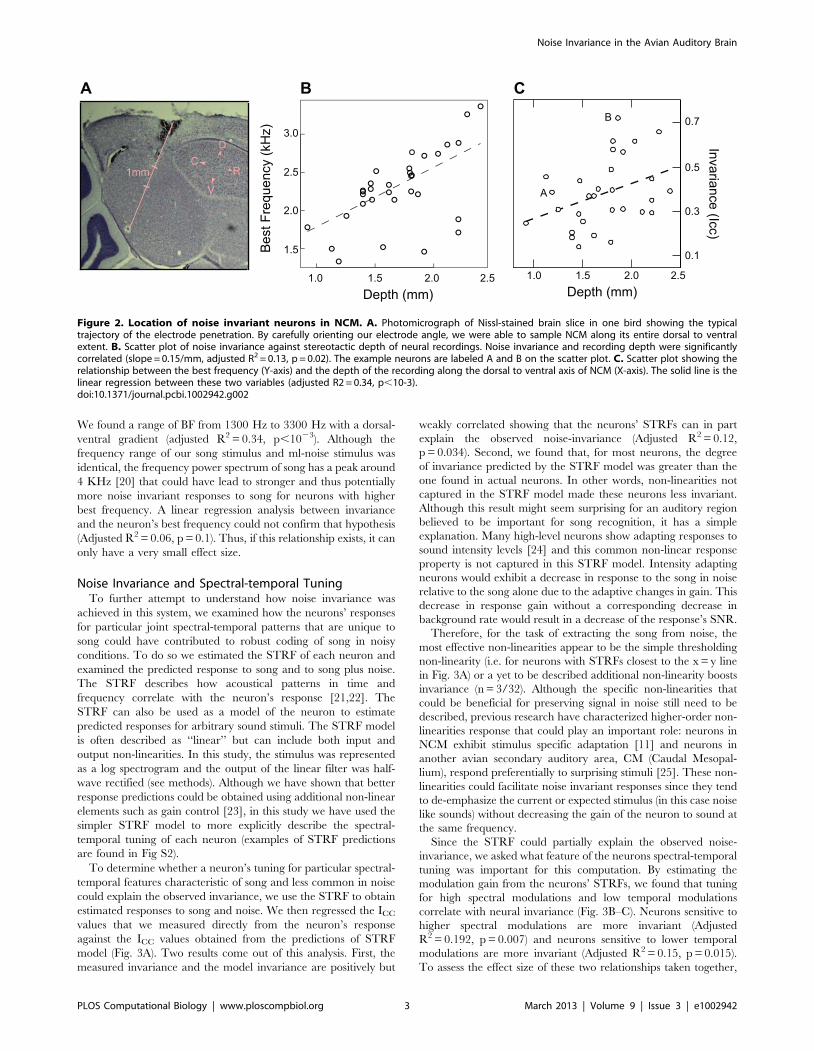
We found a range of BF from 1300 Hz to 3300 Hz with a dorsal-

ventral gradient (adjusted R2 = 0.34, p,1023). Although the

frequency range of our song stimulus and ml-noise stimulus was

identical, the frequency power spectrum of song has a peak around

4 KHz [20] that could have lead to stronger and thus potentially

more noise invariant responses to song for neurons with higher

best frequency. A linear regression analysis between invariance

and the neuron’s best frequency could not confirm that hypothesis

(Adjusted R2 = 0.06, p = 0.1). Thus, if this relationship exists, it can

only have a very small effect size.

Noise Invariance and Spectral-temporal TuningTo further attempt to understand how noise invariance was

achieved in this system, we examined how the neurons’ responses

for particular joint spectral-temporal patterns that are unique to

song could have contributed to robust coding of song in noisy

conditions. To do so we estimated the STRF of each neuron and

examined the predicted response to song and to song plus noise.

The STRF describes how acoustical patterns in time and

frequency correlate with the neuron’s response [21,22]. The

STRF can also be used as a model of the neuron to estimate

predicted responses for arbitrary sound stimuli. The STRF model

is often described as ‘‘linear’’ but can include both input and

output non-linearities. In this study, the stimulus was represented

as a log spectrogram and the output of the linear filter was half-

wave rectified (see methods). Although we have shown that better

response predictions could be obtained using additional non-linear

elements such as gain control [23], in this study we have used the

simpler STRF model to more explicitly describe the spectral-

temporal tuning of each neuron (examples of STRF predictions

are found in Fig S2).

To determine whether a neuron’s tuning for particular spectral-

temporal features characteristic of song and less common in noise

could explain the observed invariance, we use the STRF to obtain

estimated responses to song and noise. We then regressed the ICC

values that we measured directly from the neuron’s response

against the ICC values obtained from the predictions of STRF

model (Fig. 3A). Two results come out of this analysis. First, the

measured invariance and the model invariance are positively but

weakly correlated showing that the neurons’ STRFs can in part

explain the observed noise-invariance (Adjusted R2 = 0.12,

p = 0.034). Second, we found that, for most neurons, the degree

of invariance predicted by the STRF model was greater than the

one found in actual neurons. In other words, non-linearities not

captured in the STRF model made these neurons less invariant.

Although this result might seem surprising for an auditory region

believed to be important for song recognition, it has a simple

explanation. Many high-level neurons show adapting responses to

sound intensity levels [24] and this common non-linear response

property is not captured in this STRF model. Intensity adapting

neurons would exhibit a decrease in response to the song in noise

relative to the song alone due to the adaptive changes in gain. This

decrease in response gain without a corresponding decrease in

background rate would result in a decrease of the response’s SNR.

Therefore, for the task of extracting the song from noise, the

most effective non-linearities appear to be the simple thresholding

non-linearity (i.e. for neurons with STRFs closest to the x = y line

in Fig. 3A) or a yet to be described additional non-linearity boosts

invariance (n = 3/32). Although the specific non-linearities that

could be beneficial for preserving signal in noise still need to be

described, previous research have characterized higher-order non-

linearities response that could play an important role: neurons in

NCM exhibit stimulus specific adaptation [11] and neurons in

another avian secondary auditory area, CM (Caudal Mesopal-

lium), respond preferentially to surprising stimuli [25]. These non-

linearities could facilitate noise invariant responses since they tend

to de-emphasize the current or expected stimulus (in this case noise

like sounds) without decreasing the gain of the neuron to sound at

the same frequency.

Since the STRF could partially explain the observed noise-

invariance, we asked what feature of the neurons spectral-temporal

tuning was important for this computation. By estimating the

modulation gain from the neurons’ STRFs, we found that tuning

for high spectral modulations and low temporal modulations

correlate with neural invariance (Fig. 3B–C). Neurons sensitive to

higher spectral modulations are more invariant (Adjusted

R2 = 0.192, p = 0.007) and neurons sensitive to lower temporal

modulations are more invariant (Adjusted R2 = 0.15, p = 0.015).

To assess the effect size of these two relationships taken together,

Figure 2. Location of noise invariant neurons in NCM. A. Photomicrograph of Nissl-stained brain slice in one bird showing the typicaltrajectory of the electrode penetration. By carefully orienting our electrode angle, we were able to sample NCM along its entire dorsal to ventralextent. B. Scatter plot of noise invariance against stereotactic depth of neural recordings. Noise invariance and recording depth were significantlycorrelated (slope = 0.15/mm, adjusted R2 = 0.13, p = 0.02). The example neurons are labeled A and B on the scatter plot. C. Scatter plot showing therelationship between the best frequency (Y-axis) and the depth of the recording along the dorsal to ventral axis of NCM (X-axis). The solid line is thelinear regression between these two variables (adjusted R2 = 0.34, p,10-3).doi:10.1371/journal.pcbi.1002942.g002



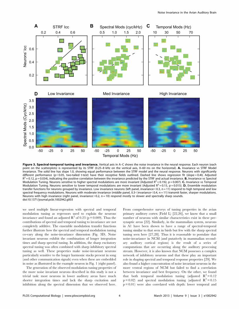
we used multiple linear-regression with spectral and temporal

modulation tuning as regressors used to explain the neurons

invariance and found an adjusted R2 of 0.23 (p = 0.009). Thus the

contributions of spectral and temporal tuning to invariance are not

completely additive. The ensemble modulation transfer functions

further illustrate how the spectral and temporal modulation tuning

co-vary along the noise-invariance dimension (Fig. 3D). Noise

invariant neurons exhibit the combination of longer integration

times and sharp spectral tuning. In addition, the sharp excitatory

spectral tuning was often combined with sharp inhibitory spectral

tuning as well. These properties make noise-invariant neurons

particularly sensitive to the longer harmonic stacks present in song

(and other communication signals) even when these are embedded

in noise as illustrated in the example neuron in Fig. 1 (right panel).

The generation of the observed modulation tuning properties of

the more noise invariant neurons described in this study is not a

trivial task: most neurons in lower auditory areas have much

shorter integration times and lack the sharp excitation and

inhibition along the spectral dimension that we observed here.

From comprehensive surveys of tuning properties in the avian

primary auditory cortex (Field L) [22,26], we know that a small

number of neurons with similar characteristics exist in these pre-

synaptic areas [22]. Similarly, in the mammalian system, neurons

in A1 have been shown to have a range of spectral-temporal

tuning similar to that seen in birds but few with the sharp spectral

tuning seen here [27,28]. Thus it is reasonable to postulate that

noise-invariance in NCM (and putatively in mammalian second-

ary auditory cortical regions) is the result of a series of

computations that are occurring along the auditory processing

stream. However, it is also known that NCM possesses a complex

network of inhibitory neurons and that these play an important

role in shaping spectral and temporal response properties [29]. We

also found a higher concentration of noise invariant neurons in the

more ventral regions of NCM but failed to find a correlation

between invariance and best frequency. On the other, we found

that both temporal modulation tuning (adjusted R2 = 0.12

p = 0.02) and spectral modulation tuning (adjusted R2 = 0.15

p = 0.01) were also correlated with depth: lower temporal and

Figure 3. Spectral-temporal tuning and invariance. Vertical axis in A–C shows the noise invariance in the neural response. Each neuron (eachpoint on the scatterplots) is represented by its STRF (0.25–8 kHz on the vertical axis, 0–60 ms on the horizontal). A. Invariance vs STRF ModelInvariance. The solid line has slope 1.0, showing equal performance between the STRF model and the neural response. Neurons with significantlydifferent performance (p,0.05, two-tailed t-test) have their receptive fields outlined. Dashed line shows regression fit (slope = 0.40, AdjustedR2 = 0.12, p = 0.034), indicating the positive correlation between the invariance predicted by the STRF and actual invariance. B. Invariance vs SpectralModulation Tuning. Neurons sensitive to higher spectral modulations are more invariant (Adjusted R2 = 0.192, p = 0.007). C. Invariance vs TemporalModulation Tuning. Neurons sensitive to lower temporal modulations are more invariant (Adjusted R2 = 0.15, p = 0.015). D. Ensemble modulationtransfer functions for neurons grouped by invariance. Low invariance neurons (left panel, invariance,0.3, n = 11) respond to high temporal and lowspectral frequency modulations. Neurons with moderate invariance (middle panel, 0.3,invariance,0.4, n = 11) transmit faster, sharper modulations.Neurons with high invariance (right panel, invariance.0.2, n = 10) respond mostly to slower and spectrally sharp sounds.doi:10.1371/journal.pcbi.1002942.g003



higher spectral modulation tuning is found in ventral regions of

NCM. This organization of tuning properties is reminiscent of the

organization of the primary auditory areas, field L, where the

output layers have a higher concentration of neurons with longer

integration times [30]. Thus both upstream and local circuitry are

almost certainly involved in the creation of noise-invariant neural

representations.

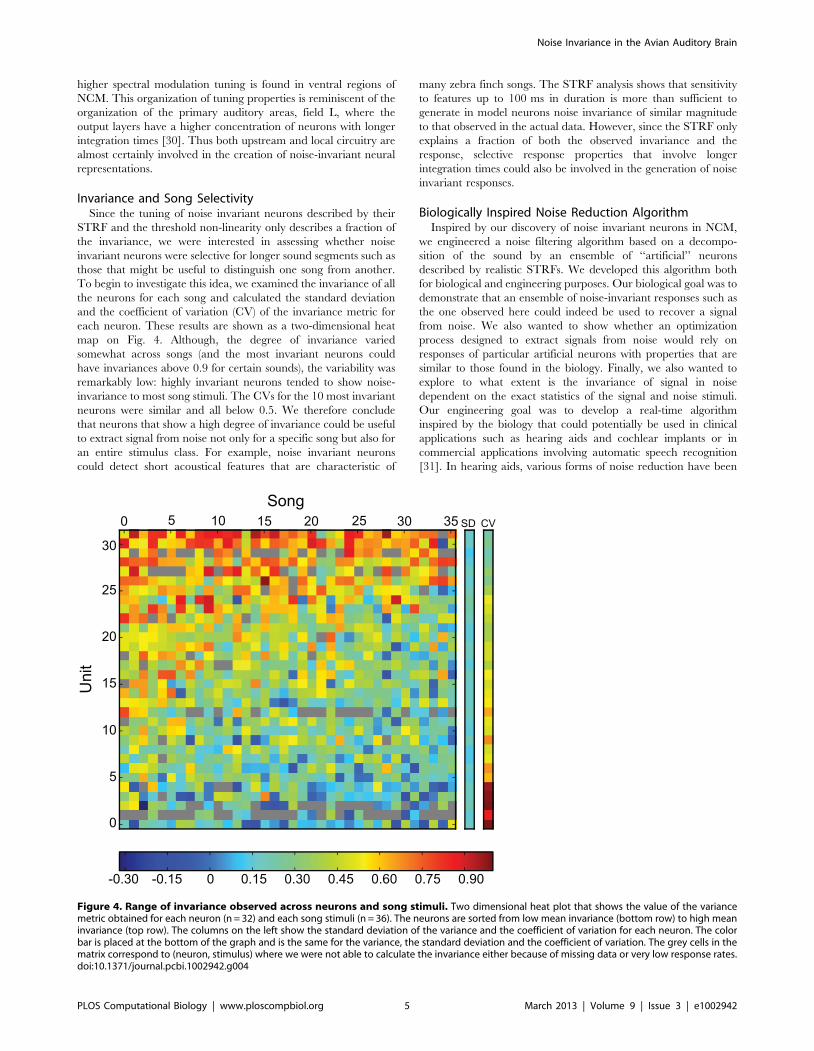
Invariance and Song SelectivitySince the tuning of noise invariant neurons described by their

STRF and the threshold non-linearity only describes a fraction of

the invariance, we were interested in assessing whether noise

invariant neurons were selective for longer sound segments such as

those that might be useful to distinguish one song from another.

To begin to investigate this idea, we examined the invariance of all

the neurons for each song and calculated the standard deviation

and the coefficient of variation (CV) of the invariance metric for

each neuron. These results are shown as a two-dimensional heat

map on Fig. 4. Although, the degree of invariance varied

somewhat across songs (and the most invariant neurons could

have invariances above 0.9 for certain sounds), the variability was

remarkably low: highly invariant neurons tended to show noise-

invariance to most song stimuli. The CVs for the 10 most invariant

neurons were similar and all below 0.5. We therefore conclude

that neurons that show a high degree of invariance could be useful

to extract signal from noise not only for a specific song but also for

an entire stimulus class. For example, noise invariant neurons

could detect short acoustical features that are characteristic of

many zebra finch songs. The STRF analysis shows that sensitivity

to features up to 100 ms in duration is more than sufficient to

generate in model neurons noise invariance of similar magnitude

to that observed in the actual data. However, since the STRF only

explains a fraction of both the observed invariance and the

response, selective response properties that involve longer

integration times could also be involved in the generation of noise

invariant responses.

Biologically Inspired Noise Reduction AlgorithmInspired by our discovery of noise invariant neurons in NCM,

we engineered a noise filtering algorithm based on a decompo-

sition of the sound by an ensemble of ‘‘artificial’’ neurons

described by realistic STRFs. We developed this algorithm both

for biological and engineering purposes. Our biological goal was to

demonstrate that an ensemble of noise-invariant responses such as

the one observed here could indeed be used to recover a signal

from noise. We also wanted to show whether an optimization

process designed to extract signals from noise would rely on

responses of particular artificial neurons with properties that are

similar to those found in the biology. Finally, we also wanted to

explore to what extent is the invariance of signal in noise

dependent on the exact statistics of the signal and noise stimuli.

Our engineering goal was to develop a real-time algorithm

inspired by the biology that could potentially be used in clinical

applications such as hearing aids and cochlear implants or in

commercial applications involving automatic speech recognition

[31]. In hearing aids, various forms of noise reduction have been

Figure 4. Range of invariance observed across neurons and song stimuli. Two dimensional heat plot that shows the value of the variancemetric obtained for each neuron (n = 32) and each song stimuli (n = 36). The neurons are sorted from low mean invariance (bottom row) to high meaninvariance (top row). The columns on the left show the standard deviation of the variance and the coefficient of variation for each neuron. The colorbar is placed at the bottom of the graph and is the same for the variance, the standard deviation and the coefficient of variation. The grey cells in thematrix correspond to (neuron, stimulus) where we were not able to calculate the invariance either because of missing data or very low response rates.doi:10.1371/journal.pcbi.1002942.g004



shown to offer an incremental improvement in the listening

experience [32,33] though listening to speech in noisy environ-

ments remains the principal complaint of hearing aid users [34]. In

addition, none of the current noise reduction algorithms have led

to improvements in speech intelligibility [35,36].

Our ensemble of artificial neurons can be thought of as a

modulation filter bank because the response of each neuron

quantifies the presence and absence of particular spectral-temporal

patterns as observed in a spectrogram and, contrary to a frequency

filter bank, not solely the presence or absence of energy at a

particular frequency band. In other words, the STRFs can be

thought of as ‘‘higher-level’’ sound filters: if lower-level sound

filters operate in the frequency domain (for example removing low

frequency noise such as the hum of airplane engines), these high-

level filters operate in the spectral-temporal modulation domain.

In this joint modulation domain, sounds that have structure in

time (such as beats) or structure in frequency (such as in a musical

note composed of a fundamental tone and its harmonically related

overtones) are characterized by specific temporal and spectral

modulations. A spectral-temporal modulation filter could then be

used to detect sounds that contain particular time-frequency

patterns while filtering out other sounds that might have similar

frequency content but lack this spectral-temporal structure.

Similar decompositions have also been proposed and used by

others for the efficient processing of speech and other complex

signals [37,38,39].

Noise filtering with such a modulation filter bank can be

described as series of signal processing steps: i) decompose the

signal into frequency channels using a frequency filter bank; ii)

represent the sound as the envelope in each of the frequency

channels, as it is done in a spectrogram; iii) filter this time-

frequency amplitude representation by a modulation filter bank to

effectively obtain a filtered spectrogram; iv) invert this filtered

spectrogram to recover the desired signal. Although each of these

steps involves relatively simple signal processing, two significant

issues remain. First, one has to choose the appropriate gain on the

modulation filters in order to detect behaviorally relevant signals

over noise. Second, the spectrogram inversion step requires a

computationally intensive iterative procedure [40] that would

prevent such a modulation filtering procedure to operate in real

time or with minimal delays. Our algorithm solves these two issues.

We have eliminated the spectrographic inversion step and instead

use the output of the modulation filter bank to generate a time-

varying gain vector that can directly operate on the output of the

initial frequency filter bank. Second, we propose to find optimal

fixed gains on the modulation filter bank by minimizing the error

between a desired signal and the output of the filtering process in

the time domain. Then once the modulation filter weights are

fixed, the algorithm can operate in real-time with a delay that is

only dependent on the width of the STRF in the modulation filter

bank.

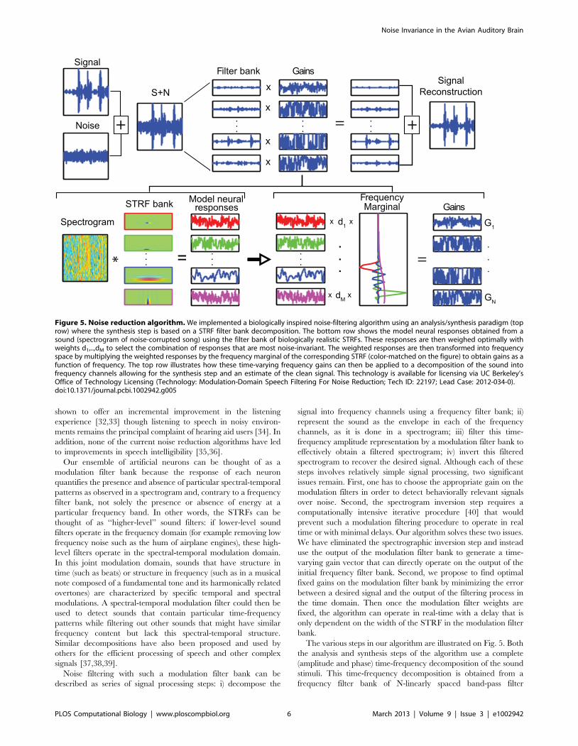
The various steps in our algorithm are illustrated on Fig. 5. Both

the analysis and synthesis steps of the algorithm use a complete

(amplitude and phase) time-frequency decomposition of the sound

stimuli. This time-frequency decomposition is obtained from a

frequency filter bank of N-linearly spaced band-pass filter

Figure 5. Noise reduction algorithm. We implemented a biologically inspired noise-filtering algorithm using an analysis/synthesis paradigm (toprow) where the synthesis step is based on a STRF filter bank decomposition. The bottom row shows the model neural responses obtained from asound (spectrogram of noise-corrupted song) using the filter bank of biologically realistic STRFs. These responses are then weighed optimally withweights d1,..,dM to select the combination of responses that are most noise-invariant. The weighted responses are then transformed into frequencyspace by multiplying the weighted responses by the frequency marginal of the corresponding STRF (color-matched on the figure) to obtain gains as afunction of frequency. The top row illustrates how these time-varying frequency gains can then be applied to a decomposition of the sound intofrequency channels allowing for the synthesis step and an estimate of the clean signal. This technology is available for licensing via UC Berkeley’sOffice of Technology Licensing (Technology: Modulation-Domain Speech Filtering For Noise Reduction; Tech ID: 22197; Lead Case: 2012-034-0).doi:10.1371/journal.pcbi.1002942.g005



Gaussian shaped channels located between 250 Hz and 8 kHz.

The amplitude of these N narrow-band signals is obtained using

the Hilbert transform (or rectification and low-pass filtering) to

generate a spectrogram of the sound. This spectrographic

transformation is identical to the one that we use for the

estimation of the STRFs (see methods).

The analysis step in the algorithm involves generating an

additional representation of the sounds based on an ensemble of

model neurons fully characterized by their STRF. These STRFs

are designed to efficiently encode the structure of the signal and

the noise, allowing them to be useful indicators of the time-course

of signal in a noisy sound. For this study, we used a bank of STRFs

that were designed to model the STRFs found throughout the

auditory pallium, including STRFs not only from neurons in

NCM but also the field L complex [22]. The log spectrogram of

the stimulus is convolved with each STRF to obtain model neural

responses: ~aa(t) of dimension M. The crux of our algorithm is to

transform these neural responses back into a set of time varying

frequency gains, ~gg(t) of dimension N. These frequency gains will

then be applied to the corresponding frequency slices in the time-

frequency decomposition of the sound to synthesize the processed

signal. ~gg(t) is a function of the sum of all model neural responses

each scaled by an importance weighting, di, and then multiplied

by the frequency marginal of the corresponding neuron’s STRF:

gj(t)~fXMi~1

di:ai(t):Ki,j

!with j[ 1,Nf g:

The function f was chosen to be the logistic function in order to

restrict the gains to lie between a lower bound, representing

maximal attenuation, and 0 dB, representing no attenuation. Ki,j

is the frequency marginal value of neuron i for the frequency band

centered at j, and it was obtained from the frequency marginal of

each STRF. Using these gains, we then synthesized a processed

signal:

ss(t)~XN

j~1

gj(t):yj(t),

where yj(t) is the narrow-band signal from the frequency filter j

obtained in the time-frequency decomposition of the song + noise

stimulus, x(t). The optimal set of weights, di, was learned by

minimizing the squared error e2(t)~(s(t){ss(t))2 through gradient

descent.

To assess the quality of our algorithm, we compared it to 3

other noise reduction schemes: the optimal classical frequency

Wiener filter for stationary Gaussian signals (OWF), a state-of-the-

art spectral subtraction algorithm (SINR) used by a hearing aid

company, and the upper bound obtained by an ideal binary mask

(IBM). The optimal Wiener filter is a frequency filter whose static

gain depends solely on the ratio of the power spectrum of the

signal and signal + noise. The state-of-the-art spectral subtraction

algorithm uses a time variable gain just as in our algorithm but

based on a running estimate of noise and signal spectrum. This

algorithm was patented by Sonic Innovations (US Patent

6,757,395 B1) and is currently used in hearing aids. The IBM

procedure used a zero-one mask applied to the sounds in the

spectrogram domain. The mask is adapted to specific signals by

setting an amplitude threshold. Ideal binary masks require prior

knowledge of the desired signal and thus can be considered as an

approximate upper bound on the potential performance of general

noise reduction algorithms [41].

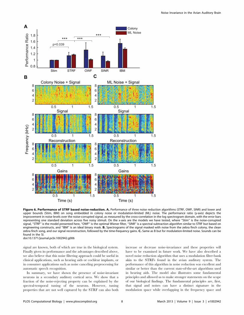
As shown on Fig. 6A, with relatively little customization and

exploration (for example in the choice of the set of artificial

STRFs) our algorithm performed strikingly well: our algorithm

performed significantly better than both the classical frequency

Wiener filter and the SINR algorithm for a song embedded in ml-

noise and similarly to the SINR algorithm for a song embedded in

colony noise. The quality of the noise filtering can also be assessed

by examining the time-varying gains shown on bottom row in

Figs 6B and C: without any a priori knowledge of the location of the

signal in time (and contrary to the IBM), the time-varying gains

can pick out when the signal occurs in the noise. Moreover, the

gains are not constant for all frequencies but instead are also able

to pick out harmonic structure in the sound. The quality of the

reconstruction can also be visually assessed by examining the

spectrograms shown in that figure or listening to the demos

provided as supplemental material.

We are now able to answer our questions. First, as quantified

above, using an ensemble of physiologically realistic noise-

invariant responses, we show that one is able to recover the

distorted signal with remarkable accuracy. Second, we were also

able to compare the properties of the STRFs in the model that had

the biggest importance gains (di) with those found in noise-

invariant neurons in NCM. As shown on Fig. 7A &B, these STRFs

are composed both of narrow band neurons with long integration

times as observed in our data set and also broad band neurons

with very short integration time. The eMTF shown in Fig. 7C&D

further quantify these results. Thus, the noise invariant neurons

found in NCM are well represented in by the model STRFs tuned

for high spectral modulation and low temporal modulations. NCM

also has neurons tuned to faster temporal modulations but the

majority of these neurons had narrow band frequency tuning (or

high spectral modulations) and these neurons are therefore not

particularly effective at rejecting noise stimuli. Fast broad-band

neurons are however found in the avian primary auditory

forebrain [22,26] and could thus play a role, as part of an

ensemble, in the signal and noise separation. Our third question

regarded the sensitivity of noise-invariant neurons to the particular

choice of signal and noise. The modeling shows that the

importance weights obtained for filtering out ml-noise were

slightly different that the weights obtained for filtering colony

noise. This relatively small effect can be visually assessed by

comparing the highest weighted STRFs for each noise class shown

in Fig. 7A versus 7B. These results suggest that slightly different

sets of invariant-neurons depending on the statistical nature of the

signal and noise but that these effects might be rather small. In

addition, we found no correlation between the magnitude of

importance weights of the artificial neurons and their BF. Thus,

we also predict that the modulation tuning properties of noise-

invariant neurons that we described here would apply to a

relatively large relevant set of natural signals and noise. This is in

part possible because many forms of environmental noise,

including noise resulting from the summation of multiple sound

signals, have similar modulation structure characterized by a

concentration of energy at very low spectral modulations and low

to intermediate temporal modulations. In converse, communica-

tion signals can have significant energy in regions combining either

high spectral modulations with low temporal modulations or high

temporal modulations with low spectral modulations [17] [42].

Both in the model and in the biological system, given a complete

modulation filter bank, the importance weights for a given signal

and noise could be learned quickly through supervised learning.

Moreover, after learning, the algorithm can easily be implemented

in real-time with minimal delay. Thus, the algorithm is particularly

useful with adaptive weights or if the statistics of the noise and



signal are known, both of which are true in the biological system.

Finally given its performance and the advantages described above,

we also believe that this noise filtering approach could be useful in

clinical applications, such as hearing aids or cochlear implants, or

in consumer applications such as noise canceling preprocessing for

automatic speech recognition.

In summary, we have shown the presence of noise-invariant

neurons in a secondary auditory cortical area. We show that a

fraction of the noise-rejecting property can be explained by the

spectral-temporal tuning of the neurons. However, tuning

properties that are not well captured by the STRF can also both

increase or decrease noise-invariance and these properties will

have to be examined in future work. We have also described a

novel noise reduction algorithm that uses a modulation filter-bank

akin to the STRFs found in the avian auditory system. The

performance of this algorithm in noise reduction was excellent and

similar or better than the current state-of-the-art algorithms used

in hearing aids. The model also illustrates some fundamental

principles and allowed us to make stronger statements on the scope

of our biological findings. The fundamental principles are, first,

that signal and noises can have a distinct signature in the

modulation space while overlapping in the frequency space and

Figure 6. Performance of STRF based noise-reduction. A. Performance of three noise reduction algorithms (STRF, OWF, SINR) and lower andupper bounds (Stim, IBM) on song embedded in colony noise or modulation-limited (ML) noise. The performance ratio (y-axis) depicts theimprovement in noise levels over the noise-corrupted signal, as measured by the cross-correlation in the log spectrogram domain, with the error barsrepresenting one standard deviation across five noisy stimuli. On the x-axis are the models we have tested, where ‘‘Stim’’ is the noise-corruptedsignal, ‘‘STRF’’ is the model presented here, ‘‘OWF’’ is the optimal Wiener filter, ‘‘SINR’’ is a spectral subtraction algorithm similar to STRF but based onengineering constructs, and ‘‘IBM’’ is an ideal binary mask. B. Spectrograms of the signal masked with noise from the zebra finch colony, the cleanzebra finch song, and our signal reconstruction, followed by the time-frequency gains. C. Same as B but for modulation-limited noise. Sounds can befound in the SI.doi:10.1371/journal.pcbi.1002942.g006



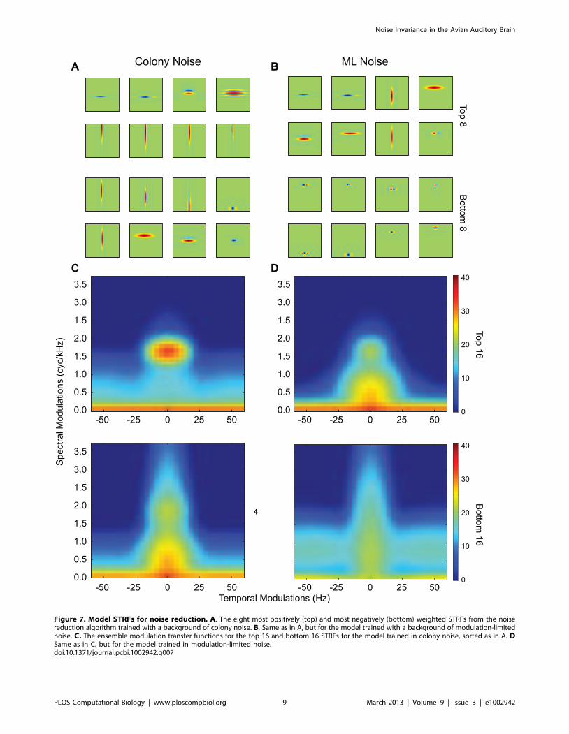
Figure 7. Model STRFs for noise reduction. A. The eight most positively (top) and most negatively (bottom) weighted STRFs from the noisereduction algorithm trained with a background of colony noise. B, Same as in A, but for the model trained with a background of modulation-limitednoise. C. The ensemble modulation transfer functions for the top 16 and bottom 16 STRFs for the model trained in colony noise, sorted as in A. DSame as in C, but for the model trained in modulation-limited noise.doi:10.1371/journal.pcbi.1002942.g007



that therefore filtering in this domain can be advantageous.

Second, that although modulation filtering is a linear operation in

the spectrogram domain, that both the generation of a spectro-

gram and the re-synthesis of a clean signal require non-linear

computations. We argue that the spectral-temporal properties that

are found in higher auditory areas and that are particularly

efficient at distinguishing noise modulations from signal modula-

tions are the result of a series of non-linear computations that

occurred in the ascending auditory processing stream. The model

also shows that a real-time re-synthesis of a cleaned signal could be

obtained with additional non-linear operations or, in other words,

that a real-time spectrographic inversion is possible. Finally, our

modeling efforts show that the noise-invariant findings described

here for a song as a chosen prototypical signal and a modulation-

limited noise as the chosen prototypical noise would also apply to

other signals and noise. However, the involvement of neurons with

slightly different tuning or adaptive properties would be needed to

obtain optimal signal detection. Given the behavioral experiments

that have shown that birds excel at auditory scene analysis tasks

both in the wild [9] and in the lab [43,44] and given our increasing

understating of the underlying neural mechanisms [45], the

birdsong model shows great promise to tackle one of the most

difficult and fascinating problems in auditory sciences: the analysis

of a sound scape into distinct sound objects.

Methods

Neurophysiology and HistologyAll animal procedures were approved by our institutional

Animal Care and Use Committee. Neurophysiological recordings

were performed in four, urethane anesthetized adult zebra finches

to obtain 50 single unit recordings in areas NCM and potentially

field L (see below). We used similar neurophysiological and

histological methods to characterize other regions of the avian

auditory processing stream and detailed descriptions can be found

there [22]. The methods are summarized here and differences

when they exist are noted.

To obtain recordings from NCM, we used more medial

coordinates than our previous experiments. With the bird’s beak

fixed at a 55u angle to the vertical, electrodes were inserted

roughly 1.2 mm rostral and 0.5 mm lateral to the Y-sinus. We

made extracellular recordings from tungsten-parylene electrodes

having impedance between 1 and 3 MV (A-M Systems).

Electrodes were advanced in 0.5 mm steps with a microdrive

(Newport), and extracellular voltages were recorded with a system

from Tucker-Davis Technologies (TDT).

In all cases, the extracellular voltages were thresholded to collect

candidate spikes. Each time the voltage crossed the threshold, the

timestamp was saved along with a high-resolution waveform of the

voltage around that time (0.29 ms before and 0.86 ms after for a

total of 1.15 ms). After the experiment, these waveforms were

sorted using SpikePak (TDT) to assess unit quality. We sorted

spike waveforms using a combination of PCA and waveform

features (maximum and minimum voltage, maximum slope, area).

We assessed clustering qualitatively and verified afterwards that

the resulting units had Inter-Spike-Interval distributions where no

more than 0.5% of the intervals were less than 1.5 ms.

In each bird, we advanced the electrode in 50 mm steps until we

found auditory responses. At that point we recorded activity in

100 mm steps. When we no longer found auditory responses, we

moved the electrode 300 mm further, made an electrolytic lesion

(2 uA610 s), advanced another 300 mm, and made a second

identical lesion. These lesions were used to find the electrode track

post-mortem and to calibrate the depth measurements.

At the end of the recording session, the bird was euthanized

with an overdose of Equithesin and transcardially perfused with

0.9% saline, followed by 3.7% formalin in 0.025 M phosphate

buffer. The skullcap was removed and the brain was post-fixed in

30% sucrose and 3.7% formalin to prepare it for histological

procedures. The brain was sliced parasagittally in 40 mm thick

sections using a freezing microtome. Alternating brain sections

were stained with both cresyl violet and silver stain, which were

then used to visualize electrode tracks, electrolytic lesions and

brain regions.

All of our electrode tracks sampled NCM from dorsal to ventral

regions. Some of the more dorsal recordings (shallower depths)

could have been in subregions L or L2b of the Field L complex as

the boundary between either of these two regions and NCM

proper is difficult to establish [46,47]. It is possible therefore that

the correlation between degree of invariance and depth also

reflects lower invariance observed in the field L complex and

higher invariance in NCM proper.

Sound StimuliStimuli consisted of zebra-finch songs, roughly 1.6–2.6 seconds

in length, recorded from 40 unfamiliar adult male zebra finches

played either in isolation or in combination with a background of

synthetic noise (song+ml-noise stimuli in main text).

The masking noise in the neurophysiological experiments was

synthetic and obtained by low-pass filtering white noise in the

modulation domain following the procedure described in [48].

This modulation low-pass filter had cutoff frequencies of vf = 1.0

cycles/kHz and vt = 50 Hz and gain roll off of 10 dB/(cycle/kHz)

and 10 dB/10 Hz. The cutoff modulation frequencies were

chosen in order to generate noisy sounds with similar range of

modulation frequencies found in environmental noise [17]. In

addition, most of the modulations found in zebra finch song are

well masked by this synthetic noise although it should be noted

that song also includes sounds features with high spectral

modulation frequencies (above 2 cycles/kHz) and high temporal

modulation frequencies (above 60 Hz). The frequency spectrum of

the ml-noise was flat from 250 Hz to 8 kHz completely

overlapping the entire range of the band-passed filtered songs

we used in the experiments. Thus, although, different results could

be found with noise stimuli with different statistics, we carefully

designed our masking noise stimulus to both capture the

modulation found in natural environmental noise while at the

same time completely overlapping the frequency spectrum of our

signal. The frequency power spectrum of these signals can be

found in [20].

We have also shown that such ml-noise is an effective stimuli for

midbrain and cortical avian auditory neurons in a sense that it

drives neuron with high response rates and high information rates

[20]. ML-noise is also very similar to the dynamic noise ripples

described in [49] and used in many neurophysiological studies to

characterize high-level mammalian auditory neurons. We also

recorded responses to the ml-noise masker alone but these data

were not analyzed for this study.

All song and ml-noise stimuli were processed to be band limited

between 250 Hz and 8 kHz and to have equal loudness using

custom code in Matlab. The sounds were presented using software

and electronics from TDT. Stimuli were played over a speaker at

72 dB C-weighted average SPL in a double-walled anechoic

chamber (Acoustic Systems). The bird was positioned 20 cm in

front of the speaker for free-field binaural stimulation.

Each of the combined stimuli consisted of a different ml-noise

sound sample, randomly paired with one of the songs. The noise

stimulus began five to seven seconds after the previous stimulus,



and the song began after a random delay of 0.5 to 1.5 seconds

after the onset of the noise. Thus for each trial the same song is

paired with a different noise sample and at a different delay. In the

combined presentations, the noise stimuli were attenuated by 3 dB

to obtain a signal to noise ratio (SNR) of 3 dB.

We played four trials at each recording location, each consisting

of a randomized sequence of 40 songs, 40 masking noise stimuli,

and 40 combined stimuli. Stimuli were separated by a period of

silence with a length uniformly and randomly distributed between

five and seven seconds.

Neural Data AnalysisWe used custom code written in MATLAB, Python and R for

all of our analyses.

We assessed responsiveness using an average z-score metric for

each stimulus class. The z-score is calculated as follows:

z~mS{mBGffiffiffiffiffiffiffiffiffiffiffiffiffiffiffiffiffiffiffiffiffiffiffiffiffiffiffiffiffiffiffiffiffiffiffiffiffiffiffiffiffiffiffiffiffiffiffiffiffiffiffi

s2Szs2

BG{2covar(S,BG)q ,

where mS is the mean response during the stimulus, mBG is the

mean response during the background, sS2 is the variance of the

response during the stimulus, and sBG2 the variance of the

response during baseline. The background rates were calculated

using the 500 ms periods preceding and following each stimulus.

Using a cutoff of z$1.5 for either ml-noise or song stimuli, 32 of

the 50 single units were determined to be responsive.

To measure invariance, we evaluated the similarity between the

responses to song and song + ml-noise by computing two

measures: 1) the correlation coefficient between the PSTH for

each corresponding response and 2) the ratio of the SNR in the

neural response to song+noise and the SNR in the response to

song alone.

If the PSTH for song is called rs(t) and the PSTH obtained in

response to song+noise is called rszn(t), then the correlation

coefficient is given by:

ICC~S rs(t){�rrsð Þ rszn(t){�rrsznð ÞTtffiffiffiffiffiffiffiffiffiffiffiffiffiffiffiffiffiffiffiffiffiffiffiffiffiffiffiffiffiffiffiffiffiffiffiffiffiffiffiffiffiffiffiffiffiffiffiffiffiffiffiffiffiffiffiffiffiffiffiffiffiffiffiffiffiffiffiffiffi

S rs(t){�rrsð Þ2Tt S rszn(t){�rrsznð Þ2Tt

q ,

where the ,. are averages across time samples. We called this

correlation coefficient, the correlation invariance or the invariance

for short. The correlation coefficient is bounded between 21 and

1 and measures the linear similarity in the response after mean

subtracted and scaling. Thus a response to song+noise with a

deviation from its mean rate that is similar in shape but much

smaller than the time-varying response to song alone will have a

very high CC invariance. A better measure of invariance might

therefore take into account both the mean PSTH rate as a proxy

for noise and the deviations from this rate as a measure of signal.

Thus, for the response to song alone, we define the signal power as

Ss~S rs(t){�rrsð Þ2T and the noise power as Ns~�rr2 for a signal to

noise ratio of:

SNRs~S rs(t){�rrsð Þ2T

�rr2s

:

For the response to the song+noise, we wanted to determine the

fraction of the time varying-response that was related to the song.

For that purpose, we used rs(t) as a regressor to obtain an estimate

of rszn(t):

rrszn(t)~b0zb1rs(t)urrszn(t)~ b0zb1�rrsð Þz b1rs(t){�rrsð Þ,

where b0 and b1 are the coefficients obtained from the normal

solution for linear regression.

The signal to noise ratio for the response to song+noise is then:

SNRszn~b2

1S rs(t){�rrsð Þ2Tb0zb1�rrsð Þ2

:

And the SNR invariance is given by the ratio of the two SNRs:

ISNR~SNRszn

SNRs

~b2

1�rr2s

b0zb1�rrsð Þ2

As shown on Fig S1A, the two metrics ended up being highly

correlated: the correlation coefficient between ICC and the log of

ISNR is r = 0.94 (p,1026) and we decided to use ICC in the main

text. However, the calculation of ISNR also provides useful

information in terms of the absolute magnitude of the invariance.

For example, it shows that the SNR in the response for the seven

most invariant cells is decreased by 5 to 10 dB when the song in

presented in noise. Thus, even for these noise-robust neurons the

loss of signal quality is present. Similarly, one can examine the

value of the linear regression coefficient, b1 on Fig S1B. This

coefficient is always less than one showing that the responses to the

song signal in the song+noise stimulus is always reduced. b1 is also

highly correlated with ICC but always smaller. Together this shows

that although the shape of the time-varying response is often very

well preserved in noise-invariant neurons, that the magnitude of

this response is decreased resulting in significant losses in signal

power (informative time-varying firing rate) relative to noise power

(mean firing rate).

In the calculations above, the PSTH was obtained by smoothing

spike arrival times using a 31 ms Hanning window. The bias

introduced by the small number of trials used to compute each

PSTH was correcting by jackknifing. The single-stimulus results

indicate a small but consistent negative bias in the four-trial

estimates. We then computed the invariance as the mean of the

individual bias-corrected correlations obtained for each 40

stimulus.

For each responsive single unit, we estimated the neuron’s

STRF from their responses to song alone. The STRF were

obtained using the strfLab neural data analysis suite developed in

our laboratory (strflab.berkeley.edu). The STRFs were estimated

by regularized linear regression. The algorithm is implemented as

a Ridge Regression in strfLab (directfit training option). Because of

the 1/f2 statistics of song, the ridge regression hyper parameter

acts as a smoothing factor on the STRF. In addition, we used a

sparseness hyper-parameter that controls the number of non-zero

coefficients in the STRF. Optimal values of the two hyperpara-

meters were found by Jackknife cross-validation (see [21,50] for

more details). The stimulus representation used for the STRF was

the log of the amplitude of the spectrogram of the sound obtained

with a Gaussian shaped filter bank of 125 Hz wide frequency

bands. Time delays of up to 100 ms were used to assess the cross-

correlation between the stimulus and the response. Performance of

the estimated final best STRF was then quantified with a separate

validation data set.

We assessed the performance of each STRF using coherence

and the normal mutual information as described in [51,52]. First,

we compute the expected coherence between two single response



trials; we then compute the coherence between the STRF

prediction and the average response. The coherence is a function

of frequency between zero and 1 that measures the correlation of

two signals at each frequency. To obtain a single measure of

correlation, one can compute the normal mutual information (MI).

We then computed the normal MI for the two coherences, calling

the first the ‘‘response information’’ and the second the ‘‘predicted

information’’. The ratio of the predicted information to the

response information is the performance ratio, and provides a

measure of model performance that is independent of the

variability of the neuron [52]. In all of our receptive field analyses,

we used only STRFs that predict sufficiently well, defined here as

having predicted information of at least 1.2 bits/second and a

performance ratio of at least 20%. The STRF performance was

not correlated with either the responsiveness of the neuron, as

measured by their z-score, or the degree of invariance (data not

shown).

To further examine the gain of the neuronal response as a

function of temporal and spectral modulations, we also represent-

ed each STRF in terms of its Modulation Transfer Function

(MTF). The MTF is obtained by taking the amplitude of 2

dimensional Fourier Transform of the STRF [42]. For each

neuron, we also computed the center of mass of its MTF to

estimate its best spectral and temporal modulation frequencies

To calculate the invariance metrics for the STRF model, we

first obtained the predicted response to the song+ml-noise stimulus

for each trial. Using these in place of the actual responses, we then

computed an invariance metrics for the STRF model by

comparing the predicted responses to the actual response obtained

for song alone. In this manner, we were able to directly compare

the STRF model invariance with the invariance calculated for the

actual neuron. We used a two-tailed t-test to compare the

distribution of similarity values for the 40, four-trial linear

predictions to the 40 actual four-trial responses.

Fig. S2 illustrates the methodology and shows the STRF, MTF,

neural responses and predictions to both song and song+ml-noise

for two additional example neurons: one with relatively low noise-

invariance and one with relatively high noise-invariance.

Noise Filtering Algorithm Using the Modulation FilterBank Model

Following directly from the premise that neurons in area NCM

selectively respond to spectral-temporal modulations present in

zebra finch songs, even in the presence of corrupting background

noise, we developed a noise reduction scheme that would exploit

this property. Our algorithm falls in the general class of single

microphone noise reduction (SMNR) algorithms using spectral

subtraction. The core idea in spectral subtraction is to estimate the

frequency components of the signal from the short time Fourier

components of the corrupted signal. The estimated signal frequency

components are obtained by multiplying the Fourier components of

signal+noise by a gain function. This is the synthesis part of the

algorithm. The gain function can vary both in frequency and time.

The form and estimation of the optimal gain function is the analysis

step of the algorithm and its design is the principal focus of the novel

development of the state-of-the art SMNR algorithms.

Both the analysis and synthesis step in our algorithm used a

complete (amplitude and phase) time-frequency decomposition of

the sound stimuli (Fig. 5). This time-frequency decomposition was

obtained from a frequency filter bank of N-linearly band-pass filter

Gaussian shaped channels located between 250 Hz and 8 kHz

(BW = 125 Hz). N was set at 60 for all simulations. The amplitude

of these N narrow-band signals could then be obtained using the

Hilbert transform to generate a spectrogram of the sound.

The analysis step in the algorithm involved generating an

additional representation of the sounds based on an ensemble of M

model neurons fully characterized by their STRF. The model

STRFs were parameterized as the product of two Gabor functions

describing the temporal and spectral response of the neuron:

STRF (t,f )~H(t):G(f ), where

H(t)~Ate{0:5 t{t0ð Þ=st½ �2 :cos(2p:Vt(t{t0)zPt) and

G(f )~Af e{0:5 f {f0ð Þ=sf

h i2

:cos(2p:Vf (f {f0)zPf ):

The parameters of these Gabor functions (e.g. for time: t0, the

temporal latency; st, the temporal bandwidth; Vt, the best

temporal modulation frequency; and Pt, the temporal phase) were

randomly chosen using a uniform distribution over the range of

those found in area NCM (present study) and Field L [22]. The

number of model neurons, M, was not found to be critical as long

as the population of STRFs sufficiently tiled the relevant

modulation space. M was set to be 140 for the results shown.

To obtain the representation of sounds in this ‘‘neural space’’, the

log spectrogram of the stimuli was convolved by each STRF to

obtain the model neural response: ~aa(t) of dimension M. As

explained in the main text, we then used these activation functions

to obtain a set of optimal time varying frequency gains, ~gg(t) of

dimension N. These frequency gains are then be applied to the

corresponding frequency slices in the time-frequency decomposi-

tion of the sound to synthesize the processed signal using:

ss(t)~XN

j~1

gj(t):yj(t),

where yj(t) is the narrow-band signal from the frequency filter j

obtained in the time-frequency decomposition of the song + noise

stimulus, x(t).

The optimal set of weights, di, needed to obtain the optimal

gains, ~gg(t) (see Results) was learned by minimizing the squared

error e2(t)~(s(t){ss(t))2 through gradient descent. For this

purpose, training stimuli were generated by summing together a

1.5 s song clip and a randomly selected chunk of either ml-noise or

zebra finch colony noise of the same duration. To match the

experimental results, both the song, s(t), and the noise, n(t), were

first high-pass filtered above 250 Hz and low-pass filtered below

8 kHz, and then resampled to a sampling rate of 16 kHz. The

song and noise were weighted to obtain a SNR of 3 dB, although

similar results were found with lower SNR’s.

Training was performed on all instances of the signal + noise

samples. Weights were determined by averaging across values

obtained through jack-knifing across this data set ten times with

10% of the data held out as an early stopping set. Noise reduction was

then validated and quantified on a novel song in novel noise.

Examples of noise corrupted signals and filtered signals that

correspond to the spectrograms shown in Fig. 6 can be found in

the supplemental online material: Audio S1, Zebra finch song masked

by ml-noise; Audio S2, the recovered song signal; Audio S3, the original

song signal; Audio S4, Zebra finch song masked by colony noise; Audio

S5, the recovered song signal; Audio S6, the original song signal.



To assess the performance of our model, we computed the cross-

correlation between the estimate and the clean signal in the log

spectrogram domain. We then took the ratio of this cross-correlation

and the value obtained prior to attempting to de-noise the stimulus to

obtain a performance ratio. As summarized in the text, we then

compared our algorithm to other noise reduction schemes. For this

purpose, we also estimated the performance ratio for three other

spectral subtraction noise algorithms: the optimal Wiener filter (OWF),

a variable gain algorithm patented by Sonic Innovations (SINR) and

the ideal binary mask (IBM). The optimal Wiener filter is a frequency

filter whose static gain depends solely of the ratio of the power spectrum

of the signal and signal + noise. In our implementation, the Wiener

filter was constructed using the frequency power spectrum of signal and

noise from the training set and then applied to a stimulus from the

testing set (of the same class). The spectral subtraction algorithm for

Sonic Innovations used a time variable gain just as in our

implementation. Also, as in our implementation, the analysis step for

estimating this gain was based on the log of the amplitude of the

Fourier components. However, the gain function itself was estimated

not from a modulation filter bank but estimating the statistical

properties of the envelope of the signal and noise in each frequency

band (US Patent 6,757,395 B1). We used a Matlab implementation of

the SINR algorithm provided to us by Dr. William Woods of Starkey

Hearing Research Center, Berkeley, CA. Optimal parameters for the

level of noise reduction and the estimation of the noise envelope for that

algorithm were also obtained on the training signal and noise stimuli

and the performance was cross-validated with the test stimuli. The

IBM procedure used a zero-one mask applied to the sounds in the

spectrogram domain. The mask is adapted to specific signals by setting

an amplitude threshold. Binary masks require prior knowledge of the

desired signal and thus should be seen as an approximate upper bound

on the potential performance of general noise reduction algorithms.

Although these simulations are far from comprehensive, they allowed

us to compare our algorithm to optimal classical approaches for

Gaussian distributed signals (OWF), to a very recent state-of-the-art

algorithm (SINR) and to an upper bound (IBM). For commercial

applications, our noise-reduction algorithm is available for licensing via

UC Berkeley’s Office of Technology Licensing (Technology: Modu-

lation-Domain Speech Filtering For Noise Reduction; Tech ID:

22197; Lead Case: 2012-034-0).

Supporting Information

Audio S1 The Zebra finch song from Audio S3 maskedby modulation limited-noise.

(WAV)

Audio S2 The recovered song signal after the corruptedsignal in Audio S1 was processed by our biologicalinspired noise-reduction algorithm.

(WAV)

Audio S3 An example of a Zebra finch song labeled as asignal since it will be masked (in Audio S1) andrecovered (in Audio S2).(WAV)

Audio S4 The Zebra finch song from Audio S6 maskedby colony noise.(WAV)

Audio S5 The recovered song signal after the corruptedsignal in Audio S4 was processed by our biologicalinspired noise-reduction algorithm.(WAV)

Audio S6 An example of a Zebra finch song labeled as asignal since it will be masked (in Audio S4) andrecovered (in Audio S3).(WAV)

Figure S1 Comparison of the correlation invariance(ICC) and the SNR invariance (ISNR). A. Scatter plot showing

the strong correlation between the ISNR (in dB units) and ICC:

r = 0.96, p,1026. B. Scatter plot between the non-normalized

linear regression coefficient, b1, and the normalized measure of

invariance, ICC. These two measures are also highly correlated:

r = 0.96, p,1026.

(EPS)

Figure S2 Example of STRF and STRF predictions fortwo cells. Column A: A low noise-invariant cell (invari-

ance = 0.25), Cell 1 and Column B: a high noise-invariant cell

(invariance = 0.65), Cell 2. Top row shows the STRF and the

corresponding MTF. Second row shows the spectrogram of one

song stimulus. Third and fourth row show the neural responses as

a spike raster (top) and a PSTH (below) to the song presented

alone. In the PSTH plot, the actual neural response is in blue and

the prediction obtained from the STRF is in red. Spike raster for

response of low noise-invariant cell to masked song. The fifth and

sixth row show the responses to the song presented over a masker

of ml-noise.

(EPS)

Acknowledgments

We thank Julie Elie and Wendy de Heer for constructive comments on a

previous version of the manuscript. We also thank William S. Woods of

Starkey Hearing Research Center, Berkeley, CA., for expert advice on

current state-of-the-art noise reduction algorithms.

Author Contributions

Conceived and designed the experiments: RCM TL FET. Performed the

experiments: RCM TL FET. Analyzed the data: RCM TL FET.

Contributed reagents/materials/analysis tools: RCM TL FET. Wrote

the paper: RCM TL FET.

References

1. Freiwald WA, Tsao DY (2010) Functional Compartmentalization and

Viewpoint Generalization Within the Macaque Face-Processing System. Science

330: 845–851.

2. Rauschecker JP, Tian B, Hauser M (1995) Processing of complex sounds in the

macaque nonprimary auditory cortex. Science 268: 111–114.

3. Sadagopan S, Wang X (2008) Level invariant representation of sounds by

populations of neurons in primary auditory cortex. Journal of Neuroscience 28:

3415–3426.

4. Billimoria CP, Kraus BJ, Narayan R, Maddox RK, Sen K (2008) Invariance and

sensitivity to intensity in neural discrimination of natural sounds. Journal of

Neuroscience 28: 6304–6308.

5. Bendor D, Wang X (2005) The neuronal representation of pitch in primate

auditory cortex. Nature 436: 1161–1165.

6. Bronkhorst AW (2000) The cocktail party phenomenon: A review of research

on speech intelligibility in multiple-talker conditions. Acustica 86: 117–

128.

7. Bee MA, Micheyl C (2008) The cocktail party problem: What is it? How can it

be solved? And why should animal behaviorists study it? Journal of Comparative

Psychology 122: 235–251.

8. Vignal C, Mathevon N, Mottin S (2004) Audience drives male songbird response

to partner’s voice. Nature 430: 448–451.

9. Aubin T, Jouventin P (2002) How to vocally identify kin in a crowd: The

penguin model. Advances in the Study of Behavior. San Diego: Academic Press

Inc. pp. 243–277.

10. Knudsen DP, Gentner TQ (2010) Mechanisms of song perception in oscine

birds. Brain and Language 115: 59–68.



11. Stripling R, Volman S, Clayton D (1997) Response modulation in the zebra

finch caudal neostriatum: relationship to nuclear gene regulation. J Neurosci 17:3883–3893.

12. Phan ML, Pytte CL, Vicario DS (2006) Early auditory experience generates

long-lasting memories that may subserve vocal learning in songbirds. Proc NatlAcad Sci U S A 103: 1088–1093. Epub 2006 Jan 1017.

13. Mello C, Nottebohm F, Clayton D (1995) Repeated exposure to one song leadsto a rapid and persistent decline in an immediate early gene’s response to that

song in zebra finch telencephalon. J Neurosci 15: 6919–6925.

14. Bolhuis JJ, Zijlstra GG, den Boer-Visser AM, Van Der Zee EA (2000) Localizedneuronal activation in the zebra finch brain is related to the strength of song

learning. Proc Natl Acad Sci U S A 97: 2282–2285.15. Narayan R, Best V, Ozmeral E, McClaine E, Dent M, et al. (2007) Cortical

interference effects in the cocktail party problem. Nat Neurosci 10: 1601–1607.16. Vignal C (2004) Background noise does not modify song-induced genic

activation in the bird brain. Behavioural Brain Research 153: 241–248.

17. Singh NC, Theunissen FE (2003) Modulation spectra of natural sounds andethological theories of auditory processing. J Acoust Soc Am 114: 3394–3411.

18. Ribeiro S, Cecchi GA, Magnasco MO, Mello CV (1998) Toward a song code:evidence for a syllabic representation in the canary brain. Neuron 21: 359–371.

19. Terleph TA, Mello CV, Vicario DS (2006) Auditory topography and temporal

response dynamics of canary caudal telencephalon. J Neurobiol 66: 281–292.20. Hsu A, Woolley SM, Fremouw TE, Theunissen FE (2004) Modulation power

and phase spectrum of natural sounds enhance neural encoding performed bysingle auditory neurons. J Neurosci 24: 9201–9211.

21. Theunissen FE, David SV, Singh NC, Hsu A, Vinje W, et al. (2001) Estimatingspatio-temporal receptive fields of auditory and visual neurons from their

responses to natural stimuli. Network: Comp Neural Syst 12: 1–28.

22. Woolley SM, Gill PR, Fremouw T, Theunissen FE (2009) Functional groups inthe avian auditory system. J Neurosci 29: 2780–2793.

23. Gill P, Zhang J, Woolley SM, Fremouw T, Theunissen FE (2006) Soundrepresentation methods for spectral-temporal receptive field estimation.

J Comput Neurosci 22: 22.

24. Dean I, Harper NS, McAlpine D (2005) Neural population coding of sound leveladapts to stimulus statistics. Nature Neuroscience 8: 1684–1689.

25. Gill P, Woolley SM, Fremouw T, Theunissen FE (2008) What’s That Sound?Auditory Area CLM Encodes Stimulus Surprise, Not Intensity or Intensity

Changes. J Neurophysiol 99: 2809–2820.26. Nagel KI, Doupe AJ (2008) Organizing principles of spectral-temporal encoding

in the avian primary auditory area field L. Neuron 58: 938–955.

27. Depireux DA, Simon JZ, Klein DJ, Shamma SA (2001) Spectral-temporalresponse field characterization with dynamic ripples in ferret primary auditory

cortex. J Neurophysiol 85: 1220–1234.28. Miller LM, Escabi MA, Read HL, Schreiner CE (2002) Spectrotemporal

receptive fields in the lemniscal auditory thalamus and cortex. J Neurophysiol

87: 516–527.29. Pinaud R, Terleph TA, Tremere LA, Phan ML, Dagostin AA, et al. (2008)

Inhibitory Network Interactions Shape the Auditory Processing of NaturalCommunication Signals in the Songbird Auditory Forebrain. J Neurophysiol 14:

14.30. Kim G, Doupe A (2011) Organized Representation of Spectrotemporal Features

in Songbird Auditory Forebrain. Journal of Neuroscience 31: 16977–16990.

31. Hermus K, Wambacq P, Van hamme H (2007) A review of signal subspacespeech enhancement and its application to noise robust speech recognition.

Eurasip Journal on Advances in Signal Processing 1: 195.32. Luts H, Eneman K, Wouters J, Schulte M, Vormann M, et al. (2010)

Multicenter evaluation of signal enhancement algorithms for hearing aids.

Journal of the Acoustical Society of America 127: 1491–1505.

33. DiGiovanni JJ, Davlin EA, Nagaraj NK (2011) Effects of Transient Noise

Reduction Algorithms on Speech Intelligibility and Ratings of Hearing Aid

Users. American Journal of Audiology 20: 140–150.

34. Palmer CV (2009) A Contemporary Review of Hearing Aids. Laryngoscope 119:

2195–2204.

35. Alcantara JI, Moore BCJ, Kuhnel V, Launer S (2003) Evaluation of the noise

reduction system in a commercial digital hearing aid. International Journal of

Audiology 42: 34–42.

36. Bentler R, Wu YH, Kettel J, Hurtig R (2008) Digital noise reduction: Outcomes

from laboratory and field studies. International Journal of Audiology 47: 447–

460.

37. Chi T, Ru P, Shamma SA (2005) Multiresolution spectrotemporal analysis of

complex sounds. The Journal of the Acoustical Society of America 118: 887.

38. Mesgarani N, Slaney M, Shamma SA (2006) Discrimination of speech from

nonspeech based on multiscale spectral-temporal modulations. Ieee Transac-

tions on Audio Speech and Language Processing 14: 920–930.

39. Klein DJ, Konig P, Kording KP (2003) Sparse spectrotemporal coding of

sounds. EURASIP Journal of Applied Signal Processing 7: 659–667.

40. Griffin DW, Lim JS (1984) Signal estimation from modified short-time Fourier

transform. IEEE Transactions on Acoustics, Speech, & Signal Processing ASSP-

32: 236–243.

41. Li Y, Wang D (2009) On the optimality of ideal binary time-frequency masks.

Speech Communication 51: 230–239.

42. Woolley SM, Fremouw TE, Hsu A, Theunissen FE (2005) Tuning for spectral-

temporal modulations as a mechanism for auditory discrimination of natural

sounds. Nat Neurosci 8: 1371–1379.

43. MacDougall-Shackleton SA, Hulse SH, Gentner TQ, White W (1998) Auditory

scene analysis by European starlings (Sturnus vulgaris): Perceptual segregation of

tone sequences. Journal of the Acoustical Society of America 103: 3581–3587.

44. Benney KS, Braaten RF (2000) Auditory scene analysis in estrildid finches

(Taeniopygia guttata and Lonchura striata domestica): A species advantage for

detection of conspecific song. Journal of Comparative Psychology 114: 174–182.

45. Bee MA, Micheyl C, Oxenham AJ, Klump GM (2010) Neural adaptation to

tone sequences in the songbird forebrain: patterns, determinants, and relation to

the build-up of auditory streaming. Journal of Comparative Physiology a-

Neuroethology Sensory Neural and Behavioral Physiology 196: 543–557.

46. Vates GE, Broome BM, Mello CV, Nottebohm F (1996) Auditory pathways of

caudal telencephalon and their relation to the song system of adult male zebra

finches (Taenopygia guttata). J Comp Neurol 366: 613–642.

47. Fortune ES, Margoliash D (1992) Cytoarchitectonic organization and

morphology of cells of the field L complex in male zebra finches (Taenopygia

guttata). J Comp Neurol 325: 388–404.

48. Elliott TM, Theunissen FE (2009) The modulation transfer function for speech

intelligibility. PLoS Comput Biol 5: e1000302.

49. Escabi MA, Miller LM, Read HL, Schreiner CE (2003) Naturalistic auditory

contrast improves spectrotemporal coding in the cat inferior colliculus. J Neurosci

23: 11489–11504.

50. Woolley SM, Gill PR, Theunissen FE (2006) Stimulus-dependent auditory

tuning results in synchronous population coding of vocalizations in the songbird

midbrain. J Neurosci 26: 2499–2512.

51. Borst A, Theunissen FE (1999) Information theory and neural coding. Nat

Neurosci 2: 947–957.

52. Hsu A, Borst A, Theunissen FE (2004) Quantifying variability in neural

responses and its application for the validation of model predictions. Network

15: 91–109.



Noise-invariant Neurons in the Avian Auditory Cortex: Hearing the Song in Noise

Documents

Transcript of Noise-invariant Neurons in the Avian Auditory Cortex: Hearing the Song in Noise