Correction. Nil Deletion.. Nil Insertion.. Nil Overwriting.. Nil AE ...
Upload
khangminh22Category
view
0download
0
SLAC—360 DE90 014869
PROPERTIES OF HADRONIC DECAYS OF THE Z BOSON*
Kathryn F. O'Shaughnessy
Stanford Linear Accelerator Center Stanford University
Stanford, California 94309
June 1990
Prepared for the Department of Energy under contract number DE-AC03-76SF00515
m
nil .&*<*
; O
i * l i f OH
B ^ S
isitiliiji
nil ii i i"' f a n .ill-
Printed in the United States of America. Available from the National Technical Information Service, U.S. Department of Commerce, 5285 Port Royal Road, Springfield, Virginia 22161. Price: Printed Copy A07, Microfiche AOl.
* Ph.D. thesis SASIE?
-ACTION OF THIS DOCUMENT IS UNLIMITED

Abstract
The decays of the Z° boson to quarks and subsequently to hadrons were first directly
observed in 1989 with the Mark II detector. This report studies the general properties
of the hadronic events in the initial data sample recorded at center-of-mass energies
near the Z° resonance (91.2 GeV).
The preliminary chapters introduce the theoretical framework and the apparatus.
A brief review is given of some features of Quantum Chromodynamics (QCD) that
are relevant to the study. Two QCD-based models that are used to help correct the
data distributions for detector effects and also for comparisons with the corrected
distributions are described. For each of the detector systems used in the analysis, the
design, operation and performance is discussed.
The next chapter describes the event selection which is designed to provide a
sample of well-measured hadronic events. The following three chapters contain the
measured data distributions. The QCD-based models with parameters tuned at
Ecm= 29 GeV describe the 91 GeV data distributions well. Each of these chapters
also shows the variation of the observables as the center-of-mass energy changes.
The event shape variables chosen for study are sphericity, aplanarity, thrust, and
the hemisphere invariant masses. The distributions at 91 GeV show that the majority
of the events are 2-jet-Iike, with most of the energy confined to two narrow cones
ii

around an axis. However, there is a significant number of events with considerable
momentum away from this axis; those topologies are attributed to events with gluon
radiation from the primary quarks.
The jet analysis begins with a description and comparison of two widely used jet
cluster algorithms. One of them is chosen to apply to the data, and the number of
jets as a function of the jet resolution parameter is measured.
The last topic consists of a study of the individual charged-particle track momenta.
The corrected charged multiplicity is derived and then compared with lower energy
values. The charged-particle inclusive distributions shown are those of the scaled
momentum, the transverse momenta to the sphericity axis in and out of the event
plane, and the rapidity.
iii

Acknowledgements
My time at Stanford has been a true learning experience. I would like to thank the
Natural Sciences and Engineering Research Council of Canada and the US Depart
ment of Energy for providing the financial support for my work here. In addition,
many people contributed to the experience both academically and socially; I would
like to acknowledge their support.
Firstly, I would like to thank the Mark II collaboration for providing a wonderful
environment to learn about particle physics. I would like particularly like to thank
the technical staff at SLAC who have patiently and good-naturedly taught me much
about the hardware aspects of a detector. I would like to list all of the physicists who
have shared their ideas and listened to mine but our author lists are long enough.
However, some people deserve special mention. I would like to thank Gary Feldman,
my advisor; John Bartelt, my office-mate, for answering innumerable questions; Dave
Coupal, Jordan Nash, Tricia Rankin and Rick Van Kooten for making work on the
FADC system so enjoyable; and Walt Innes and Tom Glanzman for passing on their
knowledge about the detector so cheerfully.
For encouraging me to join activities away from SLAC, I would like to acknowledge
my friends and fellow grad students in the Physics and Applied Physics Departments
over the years. Also the students and staff at the International Center and the
iv

members of the Dunai folk dance ensemble who helped me realize that there was
more to being here than academics.
Finally, I would like to thank my family for their continued support and encourage
ment of my seemingly endless academic career. Especially my husband and "coach",
Jerry, whose love and companionship has made these last few years much richer.
v

Contents
Abstract i»
Acknowledgements v
1 Introduction I
1.1 Theory 2
1.1.1 Standard Model 3
1.1.2 The Z° Boson 4
1.1.3 Quantum Chromodynamics 6
2 QCD Models 9
2.1 Purpose of the Models 9
2.2 Two Energy Regions 11
2.2.1 Perturbative 11
2.2.2 Fragmentation 13
2.3 Specific Models and their Implementation 15
2.3.1 BIGWIG 4.1 15
2.3.2 JETSET 6.3 16
2.4 Parameters 18
VI

3 Apparatus 20
3.1 Central Drift Chamber 22
3.1.1 Drift Chamber Design 22
3.1.2 Drift Chamber Electronics 24
3.1.3 Drift Chamber Operation 26
3.1.4 Drift Chamber Performance 26
3.2 Mark II Solenoid 31
3.3 Liquid Argon Barrel Calorimeter 32
3.3-1 Physical Description 32
3.3.2 Cryogenics System 34
3.3.3 Electronics 35
3.3.4 Performance 35
3.4 The End Cap Calorimeter 38
3.4.1 Mechanical Design 38
3.4.2 Electronics 40
3.4.3 Performance 40
3.5 Luminosity Monitors 42
3.5.1 Small Angle Monitor 42
3.5.2 Mini-Small Angle Monitor 45
3.6 Trigger 47
3.6.1 Data Trigger 48
3.6.2 Cosmic Ray Trigger 51
3.6.3 Random Trigger 51
3.7 The Extraction Line Spectrometer 52
3.7.1 Spectrometer Description 52
vii
3.7.2 Magnetic Field Monitoring 53
3.7.3 Detection of Synchrotron Radiation 53
3.7.4 Performance 56
3.8 Data Aquisition System 57
4 Event selection 61
4.1 Initial Data Sample • 61
4.2 Charged Track and Neutral Shower Cuts 62
4.2.1 Charged Track Cuts 62
4.2.2 Neutral Shower Cuts 64
4.3 Event Cuts 65
4.4 Background Estimates 66
4.4.1 Physics Backgrounds 66
4.4.2 Environment Backgrounds 67
4.5 Summary of Sample 68
4.6 Corrections 68
5 Event shapes 71
5.1 Definition of Observables 71
5.2 Observations 73
5.3 Variation with Em 78
6 Jet Multiplicity 82
6.1 Cluster Algorithms 82
6.1.1 Algorithm Descriptions 84
6.1.2 Algorithm Comparison 86
6.2 Jet Fractions 89
viii

6.3 Differential Distribution 91
7 Inclusive Charged Track Distributions 92
7.1 Charged Multiplicity 92
7.1.1 Corrections 93
7.1.2 Error calculation 95
7.1.3 Variation with Eon 96
7.2 Scaled Momentum 96
7.2.1 Results 98
7.2.2 Variation with Em 98
7.3 Transverse Momentum 101
7.3.1 Variables 101
7.3.2 Results 102
7.3.3 Variation with Em 103
7.4 Rapidity 104
7.4.1 Variable definition 104
7.4.2 Results 104
8 Conclusions 106
Bibliography 109
be

List of Tables
1 Matter-building particles in the Standard Model 3
2 The three forces described by the Standard Model and the gauge bosons
that mediate them 4
3 Relative decay fractions of the Z° to the fermions 5
4 Parameters for the QCD Monte Carlo models used 19
5 Design parameters for the central drift chamber 22
6 Orientation, width and number of strips per layer in each liquid argon
module 33
7 The outermost radius and corresponding cos 8 value for each superlayer. 64
8 Correction factors for each bin for the shape distributions S, A, (1-T). 74
9 Correction factors for each bin for the shape distributions M ' / s and
{Mlfs - Mf/s) 74
10 Results of the jet algorithm comparison at Ecm = 91 GeV 87
11 Comparison of the two algorithms as E^. is changed 88
12 Correction factors for the charged particle inclusive distributions. . . 99

List of Figures
1 Diagrams involved in the definition of a,: a) the simple vertex b) some
higher order corrections to the vertex , . 7
2 Feynman diagrams for parton generation: (a) first order corrections to
qq (b) first order qqg production (c) second order qqq'if or qqgg produc
tion and (d) some diagrams contributing to second order corrections
to qqg 12
3 Concepts v view oi a parton shower 13
4 Schematic view of the upgraded Mark II detector. The two vertex
detectors were not installed for the data sample in this report 21
5 Cell design for the central drift chamber 23
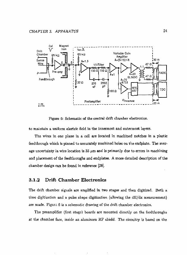
6 Schematic of the central drift chamber electronics 24
7 Tracking efficiency for the central drift chamber as a function of cos 9.
The hadronic events (boxes) are from a Monte Carlo study; the Bhabha
events (points) are from a sample of PEP data 27
8 Central drift chamber position resolution versus drift distance, with
(closed circles) and without (open circles) the time-slewing correction. . 29
XI
9 Momentum resolution for the central drift chamber. The tracks are
selected from Bhabha events and a constraint that the track originate
from a single point is used. The magnetic field was 4.5 kG 30
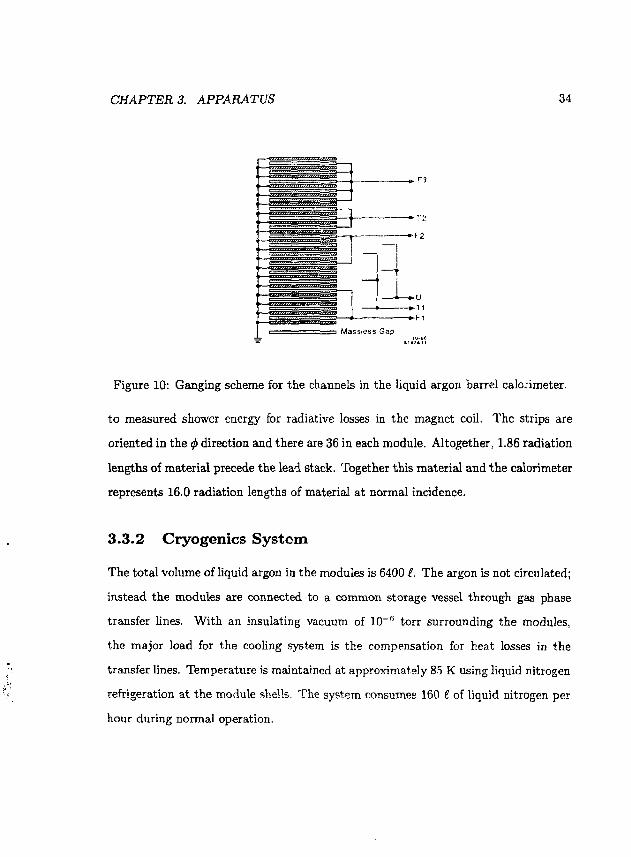
10 Ganging scheme for the channels in the liquid argon barrel calorimeter. 34
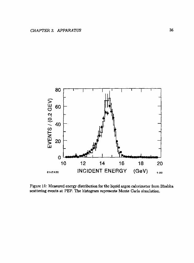
11 Measured energy distribution for the liquid argon calorimeter from
Bhabha scattering events at PEP. The histogram represents Moate
Carlo simulation 36
12 Monte Carlo simulation of the barrel calorimeter energy resolution as
a function of energy and angle of incidence 37
13 Total calorimeter thickness (in radiation lengths) (solid line) and the
number of sampling layers (dotted line) versus cos &. The shaded area
shows the region used for calculating the solid angle coverage 39
14 Response of the end cap calorimeter to small numbers (1-6) of 10 GeV
positrons 41
15 Side view of one of the four hemispherical SAM modules showing its
location inside the Mark II detector 43
16 View of two SAM modules as seen from the interaction point. The
figure shows the axes for the orientation of drift and proportional tubes
as well as the method of assembly around the beam pipe 44
17 Geometry of the Mini-SAM. As an example, in the 'Signal Used' def
inition, 12S means the signal sum of quadrants 1 and 2 being over a
Bhabha threshold in the south monitor 47
18 Block diagram of the charged particle trigger 49
19 Conceptual design of the extraction line spectrometer (ELS) system. . 52

20 Cross section of B32 magnets showing locations of magnetic strength
measuring devices for the ELS 54
21 Schematic view of the Phosphorescent Screen Monitor (PSM) 55
22 FASTBUS architecture for the Mark II data aquisition system 59
23 The distribution of transverse momentum values for data (points) and
for the MC simulation (histogram). The areas are normalized to the
number of events 63
24 The cos 6 values for tracks in the data (points) and the MC simulation
(histogram) 65
25 Feynman diagrams for the physics processes considered as background
for this analysis: a) lepton pair production and b) two-photon events. . 67
26 Corrected sphericity distribution 1/N dN/dS 75
27 Corrected 1-Thrust distribution 1/N dN/d(l-T) 76
28 Corrected aplanarity distribution 1/N dN/dA !\. i . . 76
29 Corrected scaled invariant heavy mass distribution 77
30 Corrected distribution of the difference between the scaled invariant
heavy and light masses 77
31 Mean values of sphericity (S), thrust (1-T), and aplanarity (A) versus
Ecm. The 91 GeV data values are compared with those from lower
energy e +e~ experiments; the solid lines are from the JETSET 6.3
shower model 79
32 Mean values of M\js and (Mfi/s - Mf/s) vs Ecm. The solid line is
the JETSET 6.3 shower model 80
33 End-on view of an event in the Mark II detector showing a 3-jet event. 83
xm

34 Jet fractions as a function of ycut. The solid line is from the JETSET
6.3 model, the dashed line from BIGWIG 4.1 89
35 The 3-jet fraction vs Ecm 90
36 Corrected differential jet distribution D2(y) 91
37 Multiplicity distributions. The uncorrected data is shown in (a), along
with the models after detector simulation. The result of the unfold is
shown in (b) 95
38 The corrected mean charged-particle multiplicity versus Ecm as mea
sured by e + e" experiments. The solid line is the JETSET 6.3 shower
model 97
39 Corrected \fa da/dx distribution 99
40 l/<r dojdx for a given x for various Ecm values. The solid line is from
the JETSET 6.3 shower ;aodel 100
41 Distributions of transverse momenta (a) p_i_m and (b) p±out 102
42 Mean of the squared transverse momentum distribution versus E^. . 103
43 Corrected rapidity distribution 105
xiv

Chapter 1
Introduction
The Z° boson is a recent addition to the list of observed elementary particles. A
mediator of the weak force, it was postulated in 1967 [l] and the first experimental
evidence for it was seen in proton-anti-proton collisions at the CERN laboratory near
Geneva, Switzerland, in 1983. The UA1 [2] and UA2 [3] experiments recorded events
where the reactions Z° —* e +e~ , /J"*"/!- took place.
However, the more copious decays of the Z°, namely to quarks, are too difficult
to extract from other processes happening at proton acctlerators. Therefore two
laboratories, SLAC at Stanford, CA and CERN, undertook to build machines that
would produce Zn particles through e +e~ annihilation. The SLAC Linear Collider
(SLC) was a prototype of a new type of accelerator; the CERN facility (LEP) was a
conventional storage ring accelerator at a large scale. Both machines started collecting
data in 1989. The first SLC events were recorded by the Mark II detector in April
[4] and the four detectors at LEP (ALEPH, DELPHI, L3 and OPAL) [5] all recorded
events during a short run in August and September.
Between the time that the 2" was first discovered and the first Z° events were
1

CHAPTER 1. INTRODUCTION 2
produced at SLC and LEP, a tremendous number of studies had been made by both
theorists and experimentalists. The interactions of the Z° with other particles were
predicted and the information that could be inferred about the basic theories of matter
from Z° measurements was studied [6]. It was found that Z° decays are a rich place
to look for new particles, to make precision tests of predictions of the theories, and
to learn more about areas where the theories cannot yet make predictions.
This report examines a narrow part of the second two categories. The data sample
was collected by the Mark II detector at the SLC. The general properties of the decays
of the Z° boson to quarks have been studied, concentrating on the effects of the strong
interaction which is one of the three forces that are combined in what is called the
Standard Model. The rest of this chapter a-cplains the Standard Model and what
might be learned about the strong interaction by studying hadronic decays of the Z°.
Chapter 2 describes the physics models that are used to simulate hadronic decays
and Chapter 3 discusses the general features of the Mark II detector. The method
that is used to select hadronic events based on detector measurements is described in
Chapter 4. Chapters 5-7 contain the results of the analysis, loosely divided into the
topics of event shapes, jet studies, and charged-particle inclusive studies. Chapter 8
summarizes the findings of the analysis.
1.1 Theory
It is well beyond the scope of this report to detail the complete theoretical framework
which supports the current beliefs of particle physics. In fact, only a brief summation
is offered of the concepts that affect the analysis. For more comprehensive reviews,
see [7].

CHAPTER 1. INTRODUCTION 3
Table 1: Matter-building particles in the Standard Model.
Quarks [Masses (GeV)] Charge (e) up (u) charm (c) top (r) [0.005] [1.4] [> 72]
down (d) strange(s) bottom (b) [0.007] [0.150] [4.8]
+2/3
- 1 / 3
Leptons [Masses (GeV)] electron (e~) muon (n~) tau(r~)
[0.00051] [0.1056] [1.784] e~ neutrino (i/e) yT neutrino [y^ r~ neutrino {vT) [< 0.46 x 10- 7] [< 0.50 x 10~3] [< 0.164]
- 1
0
1.1.1 Standard Model
The successful theory that integrates the electromagnetic force, the weak nuclear force
and the strong nuclear force is called the Standard Model. The first step in building
the model was the unification of the first two forces into the electro-weak theory.
This was accomplished by Glashow [8], Weinberg [1], and Salam [9] by combining
the gauge symmetry of the weak interaction, denoted SU(2) (special unitary group
with 2 dimensions) with U(l) (unitary group with dimension l) which described
electromagnetic interactions. Adding the similar gauge group description of the strong
interaction, SU(3), then provides a mathematical formulation of the three forces.
In the model there are two types of matter-building particles, quarks and leptons,
as well as force-mediating particles. The quarks and leptons are postulated to be
grouped into "generations" as shown in Table l 1 ; the different types of quarks are
said to be different "flavors". Also shown in the table are the electric charge of each 1The Standard Model set3 the number of generations to 3, but many wondered if there were
more generations at heavier masses. One of the analyses of the Z° data has shown that the number of generations with light neutrinos is less than 3.9 at a 95% confidence level flu], excluding a 4 t h
similar generation.

CHAPTER 1. INTRODUCTION 4
particle and the masses (or, if not known, mass limits). Of the particles listed, tLe
top quark has not been experimentally verified [11]. Each particle in the table has a
corresponding anti-particle partner that is not shown. The quantum numbers (e.g.
charge) are the opposite in sign for the anti-particle. The spin quantum numbers of
the quarks and leptons are half-integers, therefore they obey Fermi-Dirac statistics
and are called fermions.
The particles that mediate the forces are shown in Table 2. They have integral
spins and so are members of the class called bosons (they obey Bose-Einstein statis
tics). Another boson that is part of the Standard Model is called the Higgs boson.
Its presence is a result of the mechanism to generate masses for the particles.
1.1.2 The Z° Boson
The Z° boson, a mediator of the weak force, is the heaviest of the mediating particles
in the Standard Model. Its mass has been determined to be 91.14± 0.14 GeV [10]. It
is neutral and can decay into any fermion-anti-fermion pair with a combined mass less
than its mass (therefore all particles in Table 1 except the top quark). Table 3 shows
the relative decay fractions of the Z° to the various quarks and leptons. The ability
to observe the decay of the Z° into quarks substantially increases the possibihties for
studying the properties of the Z°.
Table 2: The three forces described by the Standard Model and the gauge bosons that mediate them.
Force Mediating particle Electromagnetic
Weak Strong
photon (7) intermediate vector bosons (Wk, Z°)
gluon (g)

CHAPTER 1. INTRODUCTION 5
Table 3: Relative decay fractions of the Z° to the fermions.
Decay Mode Percent of Decays Ve^V^^VrOr 6.1%
e + e " , [i+fi~ ,T+T~ 3.1% uu, cc, tt 10.6% dd, ss, bb 13.6%
The Z° is produced by the annihiliation of an electron (e~) and its anti-particle,
the positron (e + ). The cross section for producing the Z° peaks at center-of-rnass
energies near the Z° mass; at lower energies, e +e~ annihilation results in the produc
tion of an intermediary photon. As both the Z° and photon are neutral mediators of
the electroweak force, they both decay to fermion-anti-fermion pairs (although with
different couplings). Thus we can compare the general hadronic properties of the
Z° decays directly with those from e +e~ annihilation experiments. An advantage to
studying Z° decays is that the produced particles have higher energies.
A physics process which affects e +e~ annihilation is the radiation of a photon
by the initial e~ or e + ; the process is called initial state radiation. The result is
a lowering of the energy available to produce the intermediate state. In the case
of e^e" annihilation at Ecm= 29 GeV, the radiated photons could have energies of
several GeV. Monte Carlo (MC) programs were developed so that the energy loss
could be predicted. The presence of the Z° boson resonance makes the effect less
important. If beam energies are set to run near the peak of the resonance and either
of the initial particles emits an energetic photon, the center-of-mass energy drops
below the Z° mass where the interaction cross section is small. So these events are
rare. In any case, the process is included in the MC simulations and a correction is
made.

CHAPTER 1. INTRODUCTION 6
1.1,3 Quantum Chromodynamics
This report will be investigating particles interacting via the strong nuclear force. The
theory that describes the interaction is called Quantum Chromodynamics (QCD).
The charge carried by the particles is known as color, of which there are 3 (typically
labelled red, yellow and blue). The non-abelian nature of the theory means that the
force carriers, the gluons, also carry color and can self-interact; this has interesting
consequences.
One of the consequences is quark confinement. The gluon self-interaction causes
the force between quarks to be very strong and to rise linearly with distance. As
a quark is pulled away from other quarks (or any strongly interacting particles) a
large amount of energy is contained in the field between them and new quarks are
produced from that energy. Thus we observe combinations of quarks, not single ones.
These combinations are called hadrons and are divided into mesons (a quark and an
anti-quark) and baryons (three quarks together). An important part of QCD analyses
is estimating the effects of only observing hadrons, not the quarks and gluons.
Another consequence is seen when the coupling constant, as, is examined. The
bare coupling constant, aao, is defined at the vertex shown in Figure la. Higher order
corrections to the vertex, such as the type shown in Figure lb, cause the value of
aso to change, so a value different from the bare coupling constant is measured by
experiments. To avoid infinities in the calculation and to determine the relationship
between a5o and as, we perform a renormalization procedure and specify an energy
A which is a reference point. A result is that the value of a, depends on the energy
B* which it is being measured. To second order, the coupling constant is calculated
as: , 2» 12i
a 4 9 ; 6 Dln( gVA 2) + 6,/boln{ln(?VA2))'

CHAPTER 1. INTRODUCTION
Figure 1: Diagrams involved in the definition of as: a) the simple vertex b) some higher order corrections to the vertex.
where
b0 - (33 - 2n/)
bi = (918 - 11471/)
and n/ is the number of flavors produced at the q2 being studied. The parameter
A represents the renormalization point (the energy at which as becomes infinite)
and its value depends on the renormalization scheme. A widely used scheme is the
modified Mimimal Subtraction scheme (MS) and the corresponding parameter is
usually labelled A ^ . The value of A^JJ must be determined from experiment.
If n/ is less than 16 (which is very likely) then b0 is positive and as q2 increases,
as decreases. This trend is termed the "running" of a3 and is much more visible here
than in the corresponding description of the electromagnetic force. The difference
comes from the gluon self-interaction contributions to the diagrams. At very high
energies (q2 —> oo), as(q2) —» 0 and the strong interaction between quarks and gluons

CHAPTER 1. INTRODUCTION 8
is negligible. This effect has been termed "asymptotic freedom" [12] and implies
that perturbation theory can be used at high energies. The energy scale for the
division between the perturbative region and the non-perturbative region is set by A;
an experimental value was measured by Mark II was AJJJJ= 0.29^12^0.06 GeV using
SLC data and Am= 0.28±g;g|±S;gf GeV using PEP data [13].

Chapter 2
QCD Models
The models described in this chapter simulate the general characteristics of hadronic
events. For a given set of parameters, each model wi!l provide a set of events listing
particles and their momenta and energies. Choices about the content of individual
events are made probabilistically. Some of the parameters are determined by the
experimental situation or are known numbers {e.g. beam energy and particle masses)
and others are inherent to the particular model.
This chapter outlines the general features of models and then discusses the two
models used later in more detail.
2.1 Purpose of the Models
QCD models play an important part in experimental high energy physics. In most
currently running experiments, quark interactions are a large part of the physical pro
cesses that are occurring. Being able to simulate these interactions and the resulting
particles have the following uses.
As discussed in the next section, the simulation of hadronic events is usually
9

CHAPTER 2. QCD MODELS 10
divided into two energy regions. In the first region, at high energies, calculations
of probabilities of momentum configurations have been made. The results of those
calculations are implemented in the models using Monte Carlo techniques, and predict
the behavior of the quarks and gluons. These predictions should be measured to test
the theory of QCD.
The second energy region describes the transformation of quarks and gluons (par-
tons) to the measured hadrons. The process is not calculable using available tech
niques, so the production of hadrons (known EU "fragmentation") must be modelled.
For analyses which are trying to probe the behavior of partons, it is necessary to
investigate the effects of the fragmentation. In some cases, the parton information
is masked by the hadrons (e.g. trying to determine the direction of a quark from
the resulting hadrons (see section 6.1.2)). Many analyses turn to the models to es
timate the fragmentation effects. In addition, if the fragmentation models are based
on physics principles, the comparison of data and the models may lead to a greater
understanding of hadron production.
As well as the possibility of the models providing deeper insight to QCD and
testing its predictions, the models are also a useful tool for experimenters. Each
quantity that is measured is affected by the detector measuring it. To correct for
this, Monte Carlo simulations of the detector are written which use the particles
generated by the QCD-based models as the starting point. The detector simulation
in some ways can be thought of as a third stage of the model.
Although QCD does not often give predictions of the values of observables, it
can in some cases predict the energy evolution. When implemented in the models,
this allows the prediction of the data environment, which can have implications for
detector design. For example, at the SLC the predictions of particle multiplicities

CHAPTER 2. QCD MODELS 11
and separations helped establish criteria for track separation in the tracking devices
designed.
2.2 Two Energy Regions
The large size of the coupling constant as at low energies means that the event
simulation must be divided into two ^gions. The division occurs because ot the
calculational tools available (or lacking) to make predictions from QCD.
2.2.1 Perturbative
In the first region, the perturbative region, the quarks have such large energies that
the coupling constant is relatively small (« 0(0.10)) and so quark production can be
calculated using a perturbative series with the nth term preceeded by a coefficient
of a". Thus each successive term becomes smaller and so terminating the series or
making approximations is possible.
There are two methods which are currently used to produce the partons. The
first method, the matrix element method, uses calculations of the coefficients of the
perturbative expansion to estimate the number and 4-momenta of the produced par-
tons. At this point, only terms up to 0(a2
s) have bten calculated and confirmed and
so at most 4 partons can be produced (see Figure 2). Th.3 calculations usually make
varying assumptions (such as the procedure to recombine soft *luons) and hence some
uncertainty is introduced at this level.
The other method Is to keep the leading log terms to all orders and so it is
called the leading log approximation (LLA). In the models, it can be implemented
as a showering or cascading mechanism (see Figure 3), where at each branching a

CHAPTER 2. QCD MODELS 12
Figure 2: Feynman diagrams for parton generation: (a) first order corrections to qq (b) first order qqg production (c) second order qqq'q' or qqgg production and (d) sane diagrams contributing to second order corrections to qqg.

CHAPTER 2. QCD MODELS 13
Figure 3: Conceptual view of a parton shower.
statistical determination of the amount of momentum carried by the products is
used. This calculation is a good approximation in the case where the available energy
is quickly decreasing at each branching point.
2.2.2 Fragmentat ion
The second region of the simulation is at a low enough energy that the quarks undergo
"hadronization" or "fragmentation", that is, the confinement property causes other
quarks to be produced and hadrons to form. These hadrons are given some of the
characteristics and properties of the parent parton. Because the coupling constant is
so large at these energies, none of the calculational tools above can be used and so
models must be employed. The initial particles are a set of generated partons with
known 4-momenta. The models then use ideas based on physics principles, but not
necessarily calculations, to produce the primary hadrons.

CHAPTER 2. QCD MODELS 14
The first models used what is now called independent jet fragmentation to form
hadrons [14]. As a quark moves out from the production point, qq pairs are produced
with some fraction of the original quark's momentum. One of these quarks will
pair with the original quark and the other will continue on. This process continues
iteratively until the remaining quark has very little energy. The product quarks are
treated the same as the first quark, with no influence from previous branchings in the
chain or from other quarks (hence the description independent). Several experimental
measurements suggest that this assumption is not valid [15] and therefore independent
jet fragmentation is regarded as less accurate than some of the later models1. It will
not be discussed further in this report.
The available information about the forces between quarks suggests that the con
fining part of the strong force, F„ is governed by a term
F 3 ocfcr
where r is the distance between the quarks and k is a constant. This is the same
relationship for the force due to a string, and a model was derived [17] where the
quarks are pictured as endpoints of a string. As the quarks move apart, the string has
more energy and eventually will "break", creating two more quarks as endpoints. This
process continues until there is too little energy in the string to create more quarks.
The string then decays to hadrons. This method is known as string fragmentation,
or Lund fragmentation (from the group at Lund University that developed it).
The cluster fragmentation method takes the result of the perturbative parton
generation and forms colorless clusters of quarks. The clusters then decay according
to phase space. In later versions of the models heavy clusters decay using a string l A recent paper [16] claims than an adjustment of the treatment of soft particles can reproduce
the data, and that the independent fragmentation model is a viable model.

CHAPTER 2. QCD MODELS 15
mechanism to smaller clusters before undergoing the usual cluster decay.
2.3 Specific Models and their Implementation
The previous section briefly outlined the general concepts of the models. This section
describes the implementation of two of the more widely used QCD models. By neces
sity the discussion will be brief; these models have become very complex programs.
References [18] contain excellent reviews and comparisons of the programs.
2.3.1 BIGWIG 4.1
This model is based on ideas by Webber and Marchesini [19] and uses a parton shower
generation (the leading log approximation) and cluster fragmentation. It was the first
widely used model to use showering to generate partons.
The initial quark flavor is chosen based on the probability of coupling to the
Z°. The kinematic variables used in the showering require the choice of a reference
frame and the BIGWIG authors have chosen a frame where the initial two partons
have an opening angle of 90°. Version 4.1 also uses 0(as) calculations to weight the
momenta of this first splitting. It was found that this technique compensated for
a tendency of the shower parton generation to underestimate hard gluon radiation.
The momenta for the subsequent branchings of these partons (emitting gluons or the
gluons branching to qq pairs or to two gluons) are governed by the Altarelli-Parisi
equations [20]. The strength of the coupling constant as at each branching depends
on the parameter A as shown in Chapter 1. The evaluation of A depends on the
calculational scheme used, in this case the leading log approximation, so we label
the model parameter AfjLA. Coherence between gluons is included by a requirement

CHAPTER 2. QCD MODELS 16
that each succeeding opening angle be smaller than the previous one. The branching
piocess continues until the partons have energy below some cutoff parameter Q0 (all
the partons are considered massless at this point).
The cluster fragmentation is then implemented. Remaining gluons are forced to
break into qq pairs, and all of the quarks and anti-quarks are paired together to form
colorless clusters. An improvement over earlier versions is that if the cluster is heavier
than Mc, then the cluster fragments using a string-like mechanism before the regular
cluster decay is used. Within a cluster, a new flavor q' is chosen, and the resulting
two hadrons from the cluster will be qq' and qq'. The choice of isospin and angular
momentum for the hadron (e.g. whether a uu combination will be a TT° or a p°) is
weighted by the number of possibiUties. These hadrons then decay according to their
known decay properties. Energy and momentum conservation are forced at the end
of the generation by working backwards along the chain.
The mechanism described above only allows the creation of mesons (qq1 pairs),
whereas we know baryons (groups of three quarks or anti-quarks) are also produced
in e +e~ annihilation. The BIGWIG model forms baryons in two ways. The first
is to allow gluons to branch to diquark-anti-diquark pairs during the shower. The
second is to allow the flavor q' chosen during the cluster decay to be a diquark. With
these mechanisms, the BIGWIG model has been able to describe the observed baryon
production in the data [21].
2.3.2 JETSET 6.3
The JETSET model [22], often called the Lund model because it features the string
fragmentation developed there, has two different options for parton generation. The
default is to use 0(a2
3) matrix element calculations of the type described above.

CHAPTER 2. QCD MODELS 17
For the implementation used at Mark II, the calculations by Gutbrod, Kramer, and
Schierholz (GKS) [23] are used to predict the number and mom^u'.a <A '•.)•.•-. partons.
Again a parameter A is needed to define o^; in this case it is denoted ATJJ . In
addition, for the calculations to remain finite when soft gluons are emitted, a parton
pair resolution parameter y m t „ is used. This parameter dictates the minimum scaled
invariant mass between two partons; j / m , ; l = rnllin/s, where s = Ecm
2- The advantage
of using the matrix elements to predict parton production is that they are calculated
using well-established methods and are reliable as long as the coefficients of the higher
order corrections are small. However, they can at most give 4 partons and there are
indications that this is not adequate to describe the data at 91 GeV [21].
The version of JETSET 6.3 tha t uses parton shower generation has become one
of the more successful models for describing recent e + e~ data [21,24]. The showering
mechanism for version 6.3 is slightly different in detail from BIGWIG 4.1; the amount
of momentum the daughter particles receive at the branching is denned differently.
Also, JETSET considers the masses of the partons at each step whereas BIGWIG
calculates the masses of the partons after the cascade has finished. These differences
lie more in the implementation details rather than the fundamental idea of the shower
picture. The parameters ALLA and Qo serve the same functions as the equivalents in
the BIGWIG model.
The fragmentation parameters for the string fragmentation have the same defini
tion but will have different values for the two parton generation schemes since the
parton configuration going into the hadronization stage is different. The fragmenta
tion function, which governs the momentum sharing of the two quarks at a break in
the string, is given by
f(z)='[-{l-zrexp(=^). z z

CHAPTER 2. QCD MODELS 18
The quark direction is used in the definition of z — E + p\\, mr — yjpr + m2 is the
transverse mass of the hadron and a, b are the parameters to be determined by fits
to the data. The transverse momenta of the hadrons is given by a Gaussian function
with width a.
2.4 Parameters
The parameters of the models are in some cases well fixed by the experimental sit
uation (e.g. beam energy) and in other cases must be determined from the data.
Although the choice of values for the parameters seems to have a large range, it is
usually possible to tune them by choosing a judicious set of data distributions that
are sensitive to changes. This procedure was performed by Mark II [24] and TASSO
[25], among other experiments, using data collected at 29 GeV and 35 GeV, respec
tively. The distributions used were the same types as those studied in this analysis,
therefore it is known that they are well matched by the models at lower energies. In
Table 4 are shown the values obtained in the two studies for the two models. For this
report, the Mark II parameters tuned at 29 GeV are used for model comparisons.
If the energy variations are built into the models properly, they should be able to
predict the distributions at 91 GeV with no changes.
The difficulty with this philosophy is that a parameter for the JETSET matrix
element model cannot be sensibly used at 91 GeV. The parameter in question is
the minimum invariant mass, ymtn, which has a tuned value of 0.015. Physically the
parameter is describing the point at which we cannot resolve a soft gluon from another
parton. Practically, it is a cutoff to avoid singularities in the calculation. It defines
an absolute energy scale for the invariant mass of the partons. The remaining energy

CHAPTER 2. QCD MODELS 19
Table 4: Parameters for the QCD Monte Carlo models used,
Parameter Mark II value TASSO value JETSET 6.3 0(a;)
A;gj QCD scale 0.5 0.62 y,ntTL cutoff for combining partons 0.015 0.02
A frag function 0.9 0.58 B frag function 0.7 0.41
crq for p ± 0.265 0.40 JETSET 6.3 shower
ALZ..4 QCD scale 0.4 0.26 Qo cutoff for parton evolution 1.0 1.0
A frag function 0.45 0.18 B frag function 0.9 0.34
<7„ for p± 0.23 0.39 BIGWIG 4.1
ALL.4 QCD scale 0.75 0.25 Q0 cutoff for parton evolution 0.75 0.61
M0 for cluster cutoff 3.0 2.3
is handled by the fragmentation process and the parameters o and b. Therefore as
Erm changes, m m i n should be kept fixed in order to use the same values for a and 6.
The corresponding value of ymin at 91 GeV is 0.0015, at which point the calculations
give an unphysical negative number of 2-jet events. So the parameters tuned at 29
GeV cannot be used to generate events at 91 GeV. With the data sample presently
available, it is not possible to retune the parameters to the data; therefore this version
of the model cannot be used for comparison with the Z" hadronic data.

Chapter 3
Apparatus
The Mark II detector was upgraded in preparation for its role as the first detector
to take data at the SLAC Linear Collider (SLC) [26]. The SLC provides colliding
electron and positron beams at a centeT-of-mass energy of roughly 91 GeV. It is the
first prototype of the linear collider type of accelerator. Typical running luminosities
during the data-taking foT the analysis of this report were on the order of 10 2 8 c m " 2 s - 1 .
The SLC has only one collision point which the Mark II detector has occupied since
1986.
A schematic view of the detector can be seen in Figure 4. Emerging from the
interaction point (IP), a particle emitted perpendicular to the beam would traverse
the beampipe, the central drift chamber, a time-of-flight counter, the coil of the
solenoid magnet, the liquid argon calorimeter and finally the muon detection system.
At low angles, coverage is provided by the endcap calorimeter and the small-angle
monitor. The following sections describe the components used for the analysis. In
several cases, the performance of the components as measured at PEP is quoted; the
data sample at SLC energies is not large enough to provide a statistically meaningful
20

CHAPTER 3. APPARATUS 21
Lead/Liquid Argon Electromagnetic Calorimeter
y A
Muon Chambers
Hadron Absorber
Muon Chambers Solenoid Coil Lead-Proport ional Tube Electromagnetic Calorimeter Mini-Small Angle Monitor Small Angle Monitor Sil icon Strip Vertex Detector
Drift Chamber Vertex Detector Central Drift Chamber
Time-of-Fl ight counter
12-88 S 6147A1
Figure A: Schematic view of the upgraded Mark II detector. The two vertex detectors were not installed for the data sample in this report.

CHAPTER 3. APPARATUS 22
Table 5: Design parameters for the central drift chamber. Radius at Stereo Angle Number
Layer center (degrees) of (cm) Wirel Wire 6 cells
1 27.05 0 0 26 2 38.25 3.65 4.07 36 3 48.45 0 0 46 4 59.25 -3.73 -4.00 56 5 69.45 0 0 66 6 80.15 3.76 3.96 76 7 90.35 0 0 86 8 100.95 -3.77 -3.93 96 9 111.15 0 0 106 10 121.65 3.77 3.91 116 11 131.85 0 0 126 12 142.35 -3.78 -3.89 136
evaluation.
3.1 Central Drift Chamber
A new central drift chamber was built for the SLC run to improve the momentum res
olution, the two track separation and the pattern recognition. Some charged particle
identification capability through dE/dx measurements is also possible.
3.1.1 Drift Chamber Design
The drift chamber design is based on a six sense-wire cell, a shortened version
of the jet-chamber configuration [27]. The cells are arranged in twelve concentric
cylindrical layers, alternating between wires parallel to the cylinder axis (axial layers)
or inclined at approximately ±3.8° to the axis to provide stereo information. The

CHAPTER 3. APPARATUS 23
380 \im -Ah Offset .°
3.3 cm
1/ mm •
T-: 8.33 mm •
7.5 cm
» Sense Wire • Potential Wire o Guard Wire • Field Wire
Figure 5: Cell design for the central drift chamber.
inner radius of the drift chamber is 19.2 cm, the outer radius is 151.9 cm and the
active length is 2.30 m. The design parameters are given in Table 5.
The detailed cell design is shown in Figure 5. The sense wires (30 ^ra diameter
gold-plated tungsten) are staggered ±380 fim from the cell axis to provide local left-
right ambiguity resolution. The electric field is controlled primarily by the voltage
on a row of 19 field wires at each edge of the cell. There are also potential wires
interspersed with the sense wires and guard *ra-es which help to adjust the electric
field and the gains on the sense wires.
The wires are strung between 5.1 mm-thick aluminum endplates which are held
apart by a 2 mm-thick beryllium inner cylinder and a 1.27 mm-thick aluminum outer
shell. In addition there are eight 2.5 mm by 5.1 mm aluminum ribs attached to
the outer shell which provide structural support. The aluminum shell and beryllium
cylinder are lined with skins of copper-clad Kapton; a voltage is applied to these skins
CHAPTER 3. APPARATUS 24
Cal Magnet ~\r Iron
Drift V _ ^ ^ Chamber 05 k j l " ^ 1
Feedthrough
i 1 '1 ml r \ 1/t Filter
Test A
05 kQ
1 A.1.5
Variable Gain Amplifier
A=(0-15)1/8
1 r - H H 32 fl 2 70 2000
DF PF
Postamplifier vThreshoid T*7 i23 m
Figure 6: Schematic of the central drift chamber electronics.
to maintain a uniform electric field in the innermost and outermost layers.
The wires in one plane in a cell are located in machined notches in a plastic
feedthrough which is pinned to accurately machined holes on the endplate. The aver
age uncertainty in wire location is 35 /jm and is primarily due to errors in machining
and placement of the feedthroughs and endplates. A more detailed description of the
chamber design can be found in reference [28].
3.1.2 Drift Chamber Electronics
The drift chamber signals are amplified in two stages and then digitized. Both a
time digitization and a pulse shape digitization (allowing the dE/dx measurement)
are made. Figure 6 is a schematic drawing of the drift chamber electronics.
The preamplifier (first stage) boards are mounted directly on the feedthroughs
at the chamber face, inside an aluminum RF shield. The circuitry is based on the

CHAPTER 3. APPARATUS 25
Plessey SL560C chip. The second stage of amplification is performed by the 24-
channel postamplitiers located in crates mounted on the magnet iron. In addition,
these boards shape and split the signal. The timing half of the postamplifier has a
gain of 70 and discriminates the pulses using a LeCroy MVL407 comparator. The
threshold set for the comparator corresponds to 80 fiV at the preamp input. This is
equivalent to A% of the mean pulse height due to a minimum ionizing particle. The
gain setting for the pulse height measurement can be varied. More details on the
preamplifiers and postamplifiers can be found in reference [29].
At this point, the two sets of signals (timing and pulse shape) aTe led out approx
imately 30 m to the electronics house. The drift times are digitized by 96-channel
LeCroy 1879 TDCs located in 4 PASTBUS crates. These modules have multi-hit
capability and a time bin width of 2 ns. The drift chamber pulses are digitized by
SLAC-designed [30] FASTBUS boards. These boards are 16-charmel 100 MHz Flash
ADCs with 6-bit resolution based on the TRW 1029J7C chip.
The readout of both the TDCs and FADCs is controlled by SLAC Scanner Pro
cessors (SSPs) [31], which are programmable FASTBUS modules. One SSP is used
in each FASTBUS crate to preprocess {e.g. perform zero suppression and pedestal
corrections) and format the data. The crate SSPs are read out via cable segments by
system SSPs, which buffer the data and interface with the experiment host computer,
a VAX 8600. Programs on the host computer correlate the TDC and FADC hits on
each wire. The timing and pulse height channels are calibrated separately. For both,
the calibration pulse is injected at the input to the preamplifier. The timing calibra
tion measures the time propogation differences for each channel. The pulse height
calibration measures a pedestal, gain, and quadratic correction for each channel.

CHAPTER 3. APPARATUS 26
3.1.3 Drift Chamber Operation
A graded high voltage is supplied to the field wires of each cell through a resistor-
divider chain. The voltage on a field wire in the center of a cell is typically —4.5 kV,
the potential wire and guard wire voltages are typically —1.5 kV and —200 V respec
tively, and the sense wires are grounded. The copper skins lining the inner and outer
cylinders are typically set at —2.5 kV. The drift chamber high voltages and currents
are controlled and monitored using an IBM PC.
The chamber gas is a mixture of 89% Ar, 10% C 0 2 and 1% CH., (HRS gas) and
is at a pressure slightly above 1 atmosphere. The above voltages result in a gas gain
of approximately 2 x 10⁴ with an electric drift field of 900 V/cm and the typical drift
velocity is 52 yum/ns. For the data sample used in this report, the magnetic field was
4.75 kG, giving a Lorentz angle of 18.6°.
3.1.4 Drift Chamber Performance
Tracking Efficiency
The drift chamber tracking program utilizes the multi-sense-wire feature of the cells
and forms track segments within cells. These segments are later matched to form
tracks through the chamber [32]. The track-finding routine efficiency has been mea
sured at PEP and estimated for SLC using Monte Carlo programs. For low multi
plicity events at PEP with tracks which go through all sublayers, the efficiency was
measured to be approximately 99%. It has been estimated to be > 95% for high mul
tiplicity hadronic events at SLC energies. Figure 7 shows the efficiency as a function
of cos 8 for these two classes of events.
Position and Momentum Resolution
The position resolution in the chamber is primarily limited by diffusion in the gas.

CHAPTER 3. APPARATUS 27
1.0
o c
| 0.8
0.6 0 0.2 0.4 0.6 0.8 1.0
cos e I 6147A31
Figure 7: Tracking efficiency for the central drift chamber as a function of cos 9. The hadronic events (boxes) are from a Monte Carlo study; the Bhabha events (points) are from a sample of PEP data.

CHAPTER 3. APPARATUS 28
Calculations show that this effect contributes an error of as 150 /xm for the longest
drift distances. Other errors are w 50 fim from the time measurement error in the
electronics and » 35 fim from wire placement. When a single drift velocity was used
for all cells and layers to convert the drift times to positions, the achieved resolution
was 185 /jm. Fitting velocities for each of 3 drift distance regions in a cell and for
different groups of wire layers improved the resolution to « 170 iim.
The information from the FADCs can be included in the timing measurement by
using the deposited charge to make a "time-slewing" correction. This correction com
pensates for the change in measured time as a function of pulse height and improves
the resolution by a small amount.
Figure 8 shows the resolution versus drift distance with and without the time-
slewing correction. However, the major tracking improvement provided by the FADCs
is a better double hit separation. Scanning algorithms that use the pulse shape have
an efficiency of 80% for separating hits 2.5 mm apart compared to 5 mm if only the
TDCs are used.
Using Bhabha scattering events from PEP data in a 4.5 kG field, a momentum
resolution of a(p)/p2 = 0.46% GeV - 1 was measured in the central drift chamber for
single tracks. The resolution is tr{p)/p2 = 0.31% GeV" 1 if the tracks are constrained
to originate from a single point (see Figure 9). The multiple scattering contribution
to the resolution from the drift chamber itself is 1.4%. This number increases if
additional material from, for example, beam diagnostic devices is considered.
Particle Identification
The main purpose of the FADC system is to provide some degree of particle iden
tification, particularly for separating electrons from pions. The charge deposited by
a particle traversing the drift chamber is proportional to its energy loss (dE/dx).

CHAPTER 3. APPARATUS 29
300
CO c o o 250 £
O l -Z)
200
O 150 H LLI
100
o •
• o * ° • • ° ~ o •
• o o .
-20 0 20
DRIFT DISTANCE (mm) 6 1 4 7 A 5
Figure S: Central drift chamber position resolution versus drift distance, with (closed circles) and without (open circles) the time-slewing correction.

CHAPTER 3. APPARATUS 30
2000
5 10 15 MOMENTUM (GeV/c)
Figure 9: Momentum resolution for the central drift chamber. The tracks are selected from Bhabha events and a constraint that the track originate from a single point is used. The magnetic field was 4.5 kG.

CHAPTER 3. APPARATUS 31
The value of dE/dx coupled with the measured momentum allows a rough determi
nation of the particle mass. For a track travelling the full extent of the central drift
chamber, the 72 possible charge measurements would provide an expected dE/dx
resolution for minimum-ionizing particles of 6.9% [33]. No particle identification is
used in the analysis, so the system will not be discussed here. Reference [34] provides
more information.
3.2 Mark II Solenoid
The Mark II solenoid is a conventional cylindrical coil producing a magnetic field
of up to 5.0 kG in the center of the detector. Its thickness is 1.3 radiation lengths.
The coil consists of twelve aluminum conductors wound in series into four contiguous
cylinders. The solenoid is 405 cm long with inner and outer radii of 156 cm and 171
cm respectively. The coil can support a current of 7500 A with a total heat dissipation
of 1.8 MW.
The inner radius of the coil is covered by a heat shield which helps to isolate
it thermally from the inner detector components. A flow of 40 £ per minute of
temperature controlled water through the heat shield keeps the temperature within
the central drift chamber stable to within a few degrees. The magnetic field inside
the cylindrical volume occupied by the drift chamber has been measured and fit to
a set of polynomials in coordinates r and z. Within the tracking volume the field
is uniform to within 3% while the fit describes the magnetic field with an error of
less than 0.1%. The magnetic field used in charged particle tracking is obtained from
the fit normalized using the data from two Hall probes positioned at each end of the
central drift chamber.

CHAPTER 3. APPARATUS 32
3.3 Liquid Argon Barrel Calorimeter
The central electromagnetic calorimeter of the Mark II is a lead-liquid argon sampling
device with strip readout geometry. The calorimeter system consists of 8 independent
liquid argon cryostats enclosed in a common vacuum vessel. The system was designed
and built as part of the Mark II at SPEAR [35],
3.3.1 Physical Description
Each module measures 1.5 x 3.8 x 0.21 m 3. The modules are arranged in an octagonal
barrel outside the magnet coil. Together they cover the polar angle range of 9 =
47° to 133° and the full azimuthal angle <j> except for 3° gaps between each pair of
modules. The total solid angle coverage is 63.5%.
Each module contains a stack of alternating layers of 2 mm lead sheets and lead
strips with the 3 mm gaps between them filled with liquid argon. The lead is strength
ened with 6% antimony to minimize sagging. The strips are aligned either perpen
dicular to the beam axis to measure the polar coordinate 6, parallel tc the beam axis
to measure the azimuthal coordinate <t> or at 45" relative to the other 2 sets of strips
(labeled U) to aid in track reconstruction. Table 6 gives the details for this design.
Spacing is maintained both between strips and between layers by ceramic spacers
which contribute an overall dead space of $%. In order to reduce the number of
electronic channels many of the strips are ganged together, both from strip to strip
in certain layers and from layer to layer. The ganging results in 6 interleaved readout
layers and a total of 326 channels for each module. The ganging scheme is shown
in Figure 10. There is an additional pair of 8 mm liquid argon gaps formed by
1.6 mm thick aluminum sheets and strips in front of the lead stack to allow corrections

CHAPTER 3. APPARATUS 33
Table 6: Orientation, width and number of strips per layer in each liquid argon module.
Strip Coordinate number of strips strip width layer measured (cm)
trigger <S> 36 3.5 1 <j> 38 3.5 2 e 100 3.5 3 u 70 5.4 4 4> 38 3.5 5 e 100 3.5 6 u 70 5.4 7 4> 40 3.5 8 9 100 3.5 9 U 70 5.4 10 4> 40 3.5 11 B 100 3.5 12 e 100 3.5 13 e 100 3.5 14 4> 40 3.5 15 4> 40 3.5 16 4> 40 3.5 17 4> 40 3.5 18 <t> 40 3.5
CHAPTER 3. APPARATUS 34
* F 3
• t 2
-»T1 •»F l
Figure 10: Ganging scheme for the channels in the liquid argon barrel calorimeter.
to measured shower energy for radiative losses in the magnet coil. The strips are
oriented in the <j> direction and there are 36 in each module. Altogether,. 1.86 radiation
lengths of material precede the lead stack. Together this material and the calorimeter
represents 16.0 radiation lengths of material at normal incidence.
3.3.2 Cryogenics System
The total volume of liquid argon in the modules is 6400 £. The argon is not circulated;
instead the modules are connected to a common storage vessel through gas phase
transfer lines. With an insulating vacuum of 10~6 torr surrounding the modules,
the major load for the cooling system is the compensation for heat losses in the
transfer lines. Temperature is maintained at approximately 85 K using liquid nitrogen
refrigeration at the module shells. The system consumes 160 I of liquid nitrogen per
hour during normal operation.
Massiess Gap

CHAPTER 3. APPARATUS 35
3.3.3 Electronics
Charge produced through ionization in the liquid argon drifts to the readout strips
in a field of 12 kV/cm. Each readout strip is impedance matched to a TIS75 FET
through a small ferrite pot core transformer. The electronic noise is dominated by
Johnson noise generated in the conduction channel of the FET and is minimized using
a bipolar shaping amplifier [36] with a resolving time of 1.5 (is. The equivalent noise
energy in the ganged readout channel varies from 0.3 to 1.5 MeV and is a function of
the capacitance of the channel which varies from 0.9 to 8.0 nF. The preamplifiers and
shaping amplifiers are mounted on the detector. RF shielding encloses the modules,
the amplifiers, and the twisted pair signal cables that run from the amplifiers to the
electronics house.
Sample-and-hold modules (SHAMs [37]) follow the output voltage of the amplifiers
and are gated to hold at the peak. The charge stored in the SHAMs is measured with
12-bit ADCs incorporated in a microprocessor, BADCs [38]. The BADC in each of
the six CAMAC crates performs pedestal subtractions, linear gain corrections, and
threshold cuts. The maximum time for digitization and reduction of all data in a
CAMAC crate is 6 ms. Thresholds are normally set so that the noise occupancy is
about 5%. After ten years of operation, the number of dead channels in the system
(due to failing electronics or unrepairable internally shorted strips) is less than 1%.
3.3.4 Performance
The measured energy distribution from Bhabha scattering events at PEP is shown
in Figure 11 (the number of Bhabha events in the SLC data is too small to provide
a measurement). The resolution is cr/E = 4.6%, measured using the width of the
distribution at half maximum. However, the distribution is not Gaussian due to
CHAPTER 3. APPARATUS 36
S147A30
12 14 16 INCIDENT ENERGY
18 (GeV)
20
Figure 11: Measured energy distribution for the liquid argon calorimeter from Bhabha scattering events at PEP. The histogram represents Monte Carlo simulation.

CHAPTER 3. APPARATUS 37
I I I I I | 1 1 1 — I I I I I |
- ' * • * t * -o 8.1 ~
Angle of Incidence: • 25.0 _ a 35.7
i i i i 11 i i I
0.5 1 2 5 10 20 Incident Energy (GeV) ,_a9
Figure 12: Monte Carlo simulation of the barrel calorimeter energy resolution as a function of energy and angle of incidence.
several reasons. Dead space in the calorimeter active volume creates a low energy tail,
the size of which depends on the number of failing channels in the system. Saturation
in the readout electronics for the first active layer, used to correct for losses in the coil,
further degrades the resolution for high energy electrons in the upgrade data sample.
The gain in the amplifiers for the first layer has been reduced so that saturation does
not affect running at the SLC. As Figure 11 shows, the Monte Carlo simulation [39],
including the effects of dead space and saturation, roughly reproduces the distribution.
The energy dependence of the resolution, without saturation, has been studied with
the Monte Carlo and is shown in Figure 12. Again, these quantities are difficult to
verify with a small data sample. The position resolution measured with the PEP
V.Z5
§0.20
I 0.15 CD
1 0.10
b 0.05

CHAPTER 3. APPARATUS 38
Bhabha scattering events is 3 mrad in 4> and 0.8 cm in z and both measurements are
consistent with Monte Carlo simulation.
The inclusive electron production analysis [40] performed with data taken before
the upgrade provides an example of the electron-hadron separation capability of the
barrel calorimeter. In hadronic events, electrons were identified with an efficiency
that varied from 78% at 1 G e v / c to 93% at the highest momenta. The hadron
misidentification probability was typically 0.5% but could be as large as 3% for tracks
of momentum below 2 GeV/c ir the core of a jet. A more detailed discussion of the
performance of the barrel calorimeter can be found in previous publications [41].
3.4 The End Cap Calorimeter
The end cap calorimeters (ECC's)[42] were added to increase the electromagnetic
coverage of the detector. These lead-proportional tube calorimeters are 18 radiation
lengths (X0) thick, and cover the angular region between approximately 15° and 45°
in 9 from the beam axis. The first layer of the calorimeter is located 1.37 m in z from
the interaction point. Together with the liquid argon calorimeter, they provide full
electromagnetic calorimetry for 86% of the total solid angle (Figure 13).
3.4.1 Mechanical Design
Each ECC consists of 36 layers of 0.28 cm thick lead (0.5 X0) followed by a plane
of 191 proportional tubes. The tubes are aluminum and have a rectangular cross
section of 0.9 x 1.5cm2. The l! 1 tubes are glued together with epoxy to form an
annular plane with inner and oi ter radii of 40 cm and 146 cm. A 50 jim diameter
Stablohm 800 (nickel-chromium alloy) wire is strung through the center of each tube.

CHAPTER 3. APPARATUS 39
COS0
Figure 13: Total calorimeter thickness (in radiation lengths) (solid line) and the number of sampling layers (dotted line) versus cos 0. The shaded area shows the region used for calculating the solid angle coverage.
Alternating layers of tubes and lead are 'onded together with 0.02 cm thick epoxy-
saturated fiberglass cloth to a flatness to* -ice of 0.06 cm. The first twenty tube
planes are oriented alternately in four different d rections: vertically (X), horizontally
(Y), canted -45° (£/), and canted +45° (V). The remaining sixteen layers alternate
between X and Y layers.
The gas (HRS gas) flows at slightly above atmospheric pressure through the pro
portional tubes at a rate of one volume per two days. The outer radius of the ECC
consists of sixteen 0.16 cm thick Lexan panels, which are made gas-tight with vinyl
tape and epoxy.
To compensate for the variation of the gas gain with gas density, the temperature
is measured with thermistors embedded in each ECC and the pressure is measured
with transducers on the gas inlets and outlets. The variation of the ECC response
is less than 2% after correcting for density changes. This stability is verified by the
pulse height spectrum recorded by two small tubes that contain s s Fe sources. These

CHAPTER 3. APPARATUS 40
tubes, which are mounted on the inlet and outlet of the gas system for each ECC,
are primarily used to monitor the gas quality.
3.4.2 Electronics
The signals from several tubes are ganged together to reduce the number of elec
tronic channels to 1276 per endcap [43]. Tubes are grouped in depth and in some
cases laterally to give ten interleaved measurements of the longitudinal shower devel
opment. The ganging follows a projective geometry so that all tubes in a channel lie
approximately in a plane containing the interaction point.
The first half of the readout electronics of the ECCs consists of charge-sensitive
preamplifiers and shaping amplifiers mounted in electronics crates close to the detec
tor. These are connected to the tube anodes by coaxial cables that carry both high
voltage and signals. The second part of the system is a set of SHAM lis and BADCs
[37,38] located in the electronics building. The system is calibrated by injecting a
variable amount of charge into the front end of the preamplifiers. During readout,
pedestal and gain corrections are applied to the data and a threshold cut is made.
3.4.3 Performance
One of the ECCs was tested in a positron beam and a pion beam prior to installation.
Figure 14 shows the response of the ECC to pulses containing between one and five
10 GeV positrons. The five peaks are clearly distinguishable. The beam test data
has been used to develop algorithms that reject 99% of isolated pions while retaining
95% of electrons at a momentum of 5 GeV/c.
A study of Bhabha events in the ECCs at PEP [44] gave an energy resolution of
22%/^/E (E in GeV). Since the PEP run there has been a substantial decrease in

CHAPTER 3. APPARATUS 41
12-88
100 200 300 400 TOTAL CHARGE (pC) 6 1 4 7 A
Figure 14: Response of the end cap calorimeter to small numbers (1-5) of 10 GeV positrons.
CHAPTER 3. APPARATUS 42
the number of dead channels and an improvement in the gas tightness of the system,
so this resolution is a conservative number for the SLC data. A position resolution
of 0.7 cm in both the x and y directions was measured.
3.5 Luminosity Monitors
Two detectors whose main function is to precisely measure the integrated luminosity
have been built especially for SLC running. The Small Angle Monitor (SAM) covers
the angular range 50 mrad < 8 < 160 mrad, and the Mini-Small Angle Monitor
(Mini-SAM) covers 15 mrad < 9 < 25 mrad. Both detectors use small-angle Bhabha
scattering to measure luminosity.
3.5.1 Small Angle Monitor
Mechanical Design
The SAM consists of a tracking section with 9 layers of drift tubes and a sampling
calorimeter with 6 layers each of lead and proportional tubes (see Figure 15). Each
layer of lead is 13.2 mm thick giving a total of 14.3 radiation lengths. There are four
SAM modules, two on each side of the interaction point (IP). The distance of the
front face of the SAM from the IP is 1.38 m. Pairs of SAM modules are assembled
around the beam pipe as is shown in Figure 16. The layers are arranged in 3 different
orientations. The tubes in the first layer (Y) are horizontal and the other two layers
(U,V) are rotated ±30° from Y when looking at the front face of SAM from the IP.
For both the tracking and calorimetry layers, the pattern of layer orientation is a
series of repeating triplets YUV as seen from the IP.
Both the drift and proportional wire planes are constructed from square aluminum

CHAPTER 3. APPARATUS 43
Drift Chamber End Plate,
180 160 140 120 ,= .. Horizontal Distance from IP (cm) <,<»,«
Figure 15: Side view of one of the four hemispherical SAM modules showing its location inside the Mark II detector.
tubes 9.47 mm wide with a wall thickness of 0.25 mm. The sense wire in each tube
consists of 38 /mi diameter gold-plated tungsten. Positive high voltage is applied to
the sense wire with respect to the tube wall which is at ground potential. This voltage
is 1800V for the tracking tubes and 1700V for the calorimeter tubes. Each of the four
SAM modules contains 30 tubes per layer giving 270 tracking and 180 calorimeter cells
per module. All tubes operate with HRS gas. Since the gas gain depends strongly
on the density, the temperature and pressure of the gas are monitored by thermistors
and transducers mounted on the SAM modules.
Electronics
The electronics for the tracking part of the SAM consists of LeCroy LD604 ampli
fier/discriminators and TACs [37] that are read o- - by BADCs [38]. The calorimeter
part is instrumented with custom-designed amplifiers and the signals are stored in
SHAMs [37] which are also read out by BADCs.

CHAPTER 3. APPARATUS 44
Figure 16: View of two SAM modules as seen from the interaction point. The figure shows the axes for the orientation of drift and proportional tubes as well as the method of assembly around the beam pipe.

CHAPTER 3. APPARATUS 45
Calibration pulses are injected at the input to the amplifier with variable time
delays and constant pulse height for TACs and with constant time delay and variable
pulse heights for SHAMs. The resulting signals are fit linearly or quadratically to
extract the calibration constants which are then stored in the BADCs for subsequent
application to incoming data.
Performance
One of the four identical SAM modules was tested in a beam of positrons at 5, 10
and 15 GeV. The measured tracking resolution was 250 yxa, which yields an intrinsic
angular resolution for Bhabha tracks of 0.2 mrad assuming the SLC interaction point
is known. The measured energy resolution in the range 5-15 GeV can be parametrized
by a/E = 45%/\/E (E in GeV) for showers near the center of the SAM active
area. The resolution worsens somewhat at the edges because of radial shower leakage.
Longitudinal shower leakage increases from 9% at 5 GeV to about 22% at 50 GeV, and
fluctuations in this leakage degrade the energy resolution. The position resolution for
locating showers with just the calorimeter section of the SAM is 3 mm. This number
is used for matching tracks with showers and also represents the precision with which
photons entering the SAM can be located. The SAM Bhabha rate is estimated to be
roughly 20% higher than the visible Z° rate. The experimental systematic error on
the luminosity measurement was « 2%.
3.5.2 Mini-Small Angle Monitor
Mechanical Design
The Mini-SAM surrounds the beam pipe 2.05 m on either side of the IP. It is composed
of six layers of 0.64 cm thick scintillator interleaved with 0.79 cm-thick tungsten
slabs providing 15 radiation lengths in total thickness and resulting in an expected

CHAPTER 3. APPARATUS 46
energy resolution of 35%/Vl3 {E in GeV). The first scintillator layer is preceded
by 2 layers of tungsten (4.5 radiation lengths) as a pre-radiator. The layers are
divided into four equal azimuthal segments, each read out with a Hamamatsu R2490
photomultiplier tube viewing a wavelength shifter bar running the length of each
azimuthal segment. Angular acceptance windows are sharply defined by 5.08 cm
thick conical tungsten masks (15 radiation lengths). These masks are asymmetric;
reasons for this include allowing for motion of the interaction point without reducing
acceptance, and allowing for Monte Carlo/data disagreement at small acollinearity
angles. The angular acceptance is 15.2 mrad < 9 < 25.0 mrad on one side of the IP,
and 16.2 mrad < 9 < 24.5 mrad on the other side.
Electronics
The Mini-SAM readout electronics use a BADC -- SHAM IV combination similar to
that used by the liquid argon barrel and endcap calorimeter systems. The system also
emplys TACs [37] to provide timing information for the signals. The Mini-SAM is
read out on every trigger to monitor noise. Signals are also sent from the Mini-SAM
to the trigger logic to provide an additional Bhabha trigger.
Performance
The Mini-SAM as installed was not tested in a beam; however, a very similar pro
totype was placed in a 10 GeV e~ test beam, and these tests confirmed EGS [39]
shower studies of both the shower profile and the predicted performance of the tuDg-
sten aperture masks. A test of the integrity of the Mini-SAM has been made using
cosmic rays. The observed cosmic ray signals were used to set an approximate energy
scale for the device.
To measure luminosity, small angle Bhabha pairs must be detected above a poten
tially large machine background. All events which had > ~ 20 GeV deposited energy

CHAPTER 3. APPARATUS 47
Signal used: 12S • 23N or 23S «12N or 34S- 14N or 14S» 34N
Figure 17: Geometry of the Mini-SAM. As an example, in the 'Signal Used' definition, 12S means the signal sum of quadrants 1 and 2 being over a Bhabha threshold in the south monitor.
in both sides qualified as a Mini-SAM trigger. A Bhabha pair is defined by back-
to-back coincidences of discriminated signal sums of adjacent azimuthal segments as
shown in Figure 17. The rate of accidentals is measured by forming coincidences be
tween azimuthal segments which are not back-to-back. Other cuts are made off-line
(e.g. requiring the timing to be consistent with an e + or e" entering the front side
of the segment) to obtain the corrected luminosity. The tungsten masks defining the
angular acceptance result in a Mini-SAM Bhabha rate of approximately eight times
the total estimated visible Z° rate at i/s = Mz-
3.6 Trigger
The trigger used for running at the SLC combines a modification of the trigger used
at PEP with new FASTBUS based logic. The SLC beam crossing rate was 10, 30 or
60 Hz for the sample collected for this report. Since this allowed sufficient time to
run the trigger logic on every beam crossing, the beam crossing signal supplied by

CHAPTER 3. APPARATUS 48
the accelerator provided the primary trigger. The interface between the trigger logic
and the host VAX is provided via CAMAC by the Master Interrupt Controller (MIC)
module. Details of the trigger combination for the data sample collected are given in
section 4.1.
3.6.1 Data Trigger
There are three components of the normal data trigger. They use information from the
central drift chamber, electromagnetic calorimeters and small-angle monitors. Each
component operates independently and provides a degree of redundancy to assist in
monitoring the performance of the other components. This redundancy is also used
to measure their relative triggering efficiencies.
Charged Particle Trigger
The chaTged particle trigger uses a fast track-finding processor [45,46] to count the
number of charged tracks traversing the drift chamber. Pattern recognition can be
done with up to 12 detector layers; for this data sample, the twelve layers of the
central drift chamber were used. No information about the z-coordinate is used.
This design requires approximately 60 fis to count the charged tracks.
A drift chamber cell is considered "hit" when at least four of the six sense wires in
the cell have signals detected by the TDCs. (The number of wires which determine a
hit is programmable.) This requirement is a powerful means of rejecting backgrounds
which do not produce track segments. Requiring a track to traverse more than half a
cell produces a geometrical inefficiency of less than 0.5% for tracks of pt ~ 1 GeV/c.
The pattern of hits in each layer is loaded into a shift register and transferred
serially into special hardware curve-finding or "curvature" modules as shown in Fig
ure 18. Each curvature module is programmed to identify patterns of hits falling

CHAPTER 3. APPARATUS 49
Shift Register ^^^Tionnni
ShiH Registers
12 IB
X I Track
Counter X
Curvature Modules
Track Counter
Co planar
In Track Finder 1
MIC Start Maste Clock K> Timing Signals
to all Modules Shown
Figure 18: Block diagram of the charged particle trigger
within a specific range of radii of curvature called a road. These modules can also be
programmed to require any pattern of layers to define a valid track.
Track counters are used to record the total number of tracks found as well as
the azimuth of each track. All tracks found by curvature modules within ~ 10° in
azimuth of each other are counted as a single track. The total number of tracks found
is encoded into two bits which are passed to the MIC for the trigger decision.
Finally, a coplanar track finder is used to look specifically for back-to-back tracks.
It uses two curvature modules to estimate the azimuth of tracks, and returns a bit to
the MIC when a pair of tracks are found that are coplanar to within ~ 11°.
Calorimeter Energy Trigger
The calorimeter energy trigger uses a table of constants stored in a memory module
to find events with topologies of interest. The event topology is defined by thresholds
placed on the energy deposited in the liquid argon, endcap and SAM calorimeters,
and in small-angle counters.
A programmable Memory Logic Module (MLM) encodes 32 input bits into two
output bits which are returned to the MIC; this requires a few hundred nanoseconds.

CHAPTER 3. APPARATUS 50
The MLM uses information from the SAM and Mini-S AM to form a low-angle Bhabha
trigger for luminosity monitoring, while calorimeter information is used for the Total
Energy Deposition (TED) trigger. The TED trigger uses groups of eight adjacent
channels (strips in the liquid argon calorimeter; proportional tubes in the endcap)
which are summed at the detector. The sum representing one LA module is compared
with a threshold voltage by a strobed discriminator [47]. The sum for an endcap is
fed into two discriminators with different thresholds. The determination of these
thresholds is ultimately limited by the maximum trigger rate permitted by t'jt. data
acquisition system.
SSP-based Software Trigger(SST)
The SST was more recently designed to duplicate the capability of the TED trigger
and, in addition, to provide new software flexibility for improving both its noise sen
sitivity and pattern recognition characteristics. The redundancy available to the two
triggers does, in addition, provide an important cross check for calorimeter triggering.
A SLAC Scanner Processor (SSP) is the component of the SST which processes the
calorimetric data in a much more flexible manner than the TED trigger. Copies of
the LA and EC trigger sums are made by summing/buffer boards which are then
digitized by LeCroy 1885N FASTBUS ADCs. In one pass the SSP reads out the
ADCs and defines "hits" based on three software thresholds. Trigger algorithms then
find calorimetric "towers" (clusters of energy which point to the IP) by using the
hits to index a table of pre-calculated patterns. (The complexity of the algorithm is
constrained only by the time available between beam crossings.) Only the energies of
the channels contributing to a tower are summed, therefore the SST eliminates noise
from other channels in the modules. More details on the SST system may be found
in reference [48]. For most of the data-taking run, the single tower energy threshold

CHAPTER 3. APPARATUS 51
was 2.2 GeV for the LA system and 3-3 GeV for the endcaps.
In addition to the calorimeters, the SST reads out noise monitors through its
ADCs. There are 48 ionization chambers in the last section of the SLC beamline,
and 16 proportional tubes along the beamline in the experimental hall (and inside
the Mark II). An increase in the signals from these monitors is indicative of various
accelerator-related problems such as klystron tube and magnet failures or mis-steering
of the beams.
3.6.2 Cosmic Ray Trigger
A cosmic ray trigger is needed for debugging and performance evaulation of individ
ual detector components. Cosmic rays are defined using the normal charged particle
trigger system in conjunction with a signal from the TOF system to provide an abso
lute time measurement required by the charged trigger electronics and drift chamber
reconstruction software. Cosmic ray data also form an important check of the charged
particle trigger performance.
3.6.3 Random Trigger
To monitor the accelerator backgrounds, a random trigger was developed. Pre-scaled
to provide a low percentage of the triggers, the events which have only the random
trigger are very useful in estimating the energy deposition in the detector when no
annihilation occurred. See section 4.4.2 for details of the use of these events.

CHAPTER 3. APPARATUS 52
Spectrometer Quadrupole Magnet
Doublet Vertical
Dump Synchrotron Light Monitor
2-90 5771A1
Figure 19: Conceptual design of the extraction line spectrometer (ELS) system.
3.7 The Extraction Line Spectrometer
In order to determine the center-of-mass energy (Ecm) at the SLC interaction point
(IP), precise measurements of the beam energies (Ebeam) for both the e~ and e + beams
are essential. To meet the resolution goal of a-^Si- < 0.05%, precision sper -^meters
were installed [49] in the SLC extraction lines, 150 m downstream of the Ii" in both
beam lines.
3.7.1 Spectrometer Description
A conceptual design of the extraction line is shown in Figure 19. In the line, the e*
bunch travels thro-igh a si. * e of three dipole magnets (B31, B32, and B33). Magnet
B32 is a well measured spectrometer magnet (set at / Bdl = 30.5 kG • m when Et,eam is
50 GeV) which bends the beam by an amount proportional to / Bdl/EiJMm. Magnets
B31 and B33 bend the beam perpendicular to the bend direction of B32 and cause
the beam to emit two 5 cm wide swaths of synchrotron radiation. Synchrotron light
detectors located at the beam focal point (approximately 15 m from B32) measure
the distance between these swaths (approximately 27 cm) and thus the angle through

CHAPTER 3. APPARATUS 53
which the beam has been bent by magnet B32. Combining this information with the
strength of the magnet allows a determination of the energy of the beam. Analysis
of the widths of the synchrotron stripes yields the energy spread of the beam.
3.7.2 Magnetic Field Monitoring
Two high prei.; in, absolute methods were used to make a determination of the
magnetic strength of the B32 magnets before their installation in the extraction line.
The first measured / Bdl directly by moving NMR probes along the length of the
magnet, measuring B and dl for each step. In the second method, / Bdl was measured
by monitoring the voltage induced on a moving loop of wire. These methods are
described in detail elsewhere [50]. The techniques agreed to better than 0.008%.
The absolute measurements were used to simultaneously calibrate three online
methods of determining the spectrometer strength: a flip coil, NMR probes, and
current monitors. A cross section of the magnet with these devices installed in the
gap is shown in Figure 20. Agreement between the flip coil and NMR probes was
better than 0.01%.
3.7.3 Detection of Synchrotron Radiation
The bend magnets cause the beam to emit intense swaths of synchrotron radiation
with a maximum energy of approximately 3.0 MeV. An energy spread of 0.2% in the
bunches causes the stripe from B33 to be dispersed by about 540 fan at the detector
plane. Two independent detectors have been built to detect the separation and width
of the two synchrotron swaths: a Phosphorescent Screen Monitor (PSM) (Figure 21)
and a Wire Imaging Synchrotron Radiation Detector (WISRD) which was not used
during this run.
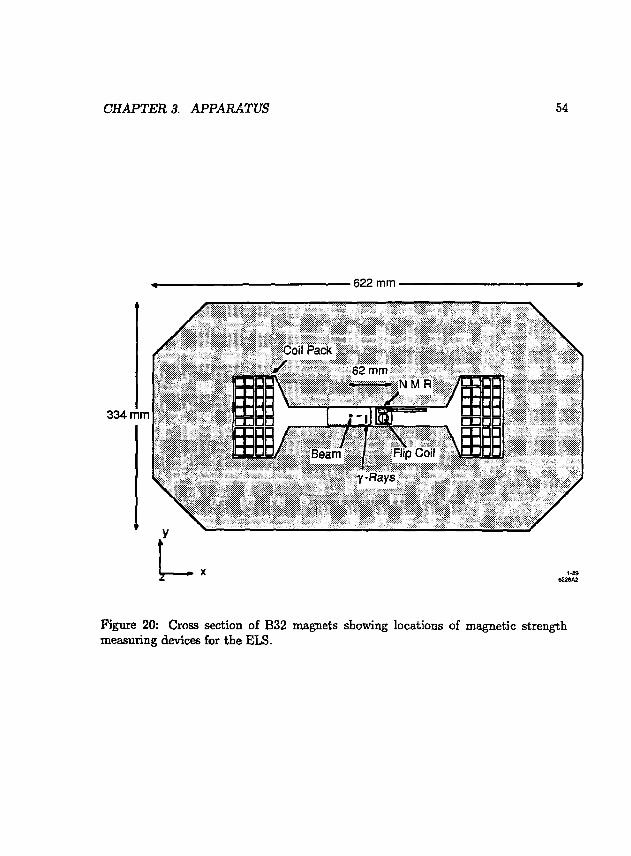
CHAPTER 3. APPARATUS 54
• 622 mm •
334 mm
Coil Pack * 62 mm
Beam } Flip Coil
7-Rays
1.89 6226A2
Figure 20: Cross section of B32 magnets showing locations of magnetic strength measuring devices for the ELS.

CHAPTER 3. APPARATUS 55
Camera
Illumination Unit
Iris Control
Phosphor Screen and Mirror /W i re Array
<ff Spectrometer Beam Deflection
Beam Pipe
Synchrotron Band
3-88 5973A1
Figure 21: Schematic view of the Phosphorescent Screen Monitor (PSM).

CHAPTER 3. APPARATUS 56
The PSM consists of two identical target and camera systems to monitor both
stripes simultaneously. An Invar [51] support structure holds both targets and fixes
the distance between them. Each target consists of an array of 100 ^m diameter
fiducial wires with center-to-center spacing of 500 fira. and a phosphorescent screen
which emits light where struck by the synchrotron beam [52j. The individual wires and
the spacing between the two arrays were measured on precision optical comparators
to an accuracy of better than 10 /xm. A camera system records both the fiducial wires
and the synchrotron stripe which runs parallel to them. The video frame is digitized
and compressed by a signal averager into a one dimensional array (perpendicular to
the wire direction) before readout. Ultimate system resolution has been measured to
be better than 25 fan. and readout rates up to SLC design repetition rate (180 Hz)
are possible.
3.7.4 Performance
In addition to the previously described errors, there are other contributions to the
error on measuring Ebeam • These contributions include: the survey of distance and
misalignments between B32 and the detectors, and misalignments between bend mag
nets. Combining these contributions in quadrature yields an estimated total error on
Ebeam of 15 MeV. However, knowledge of the average energy of the beam bunch does
not necessarily determine the luminosity weighted Eon at the IP. Complete under
standing of correlations between particle position and energy in the two colliding
bunches is essential to limit the systematic error on the energy measurement. An
absolute accuracy of 35 MeV on Et± has been achieved.

CHAPTER 3. APPARATUS 57
3.8 Data Aquisition System
Data acquisition for the Mark II detector is performed by a system of software and
hardware elements. The software consists of a number of independent processes
running on the host VAX 8600 under the control of the VMS operating system. Each
process performs a primary function and communicates with the other processes via
shared memory (global) variables, shared instructions and a form of interprocess
communication known as event flags. These functions include: reading CAMAC
data; reading FASTBUS data; merging of raw data with results from on-line event
tagging; tape logging of data records; disk logging of tagged data records; monitoring
of detector performance, electronics and environmental status; on-line analysis and
histogramming; and operator control of the experiment.
All data from the detector are channeled into the VAX through either the CA
MAC or FASTBUS interfaces. The amount of data read per event varies with the
event topology. A Z° decaying into 20 charged particles will typically result in ap
proximately 50 kbytes of data.
The CAMAC interface is a UNIBUS-based microprocessor system called the VAX
CAMAC channel or VCC [53]. This system is capable of transferring 24 bits of data
every 2 fjs. Generally, however, only the least significant 16 bits are used resulting
in a transfer rate of 1 Mbyte/s. The VCC operates a parallel branch serving two
system crates [54]. These system crates contain a total of 11 branch drivers which
connect with the 44 data acquisition crates. Event triggers are generated within the
CAMAC system and are posted as AST (Asynchronous System Trap) interrupts on
the VAX. CAMAC event acquisition consists of multiple VAX reads of individual
BADC memories and other general instrumentation modules.
The FASTBUS system interface consists of two parts. The first part is a DEC

CHAPTER 3. APPARATUS 58
DR-780 32-bit parallel port which connects the VAX SBI (Synchronous Backplane
Interconnect) with a DDI (DR-32 Device Interconnect) cable. This DDI cable con
nects with another interface [55] which provides access to a FASTBUS crate segment
through a simple buffer module, BAFFO (see Figure 22). The combined interface sup
ports interrupt messages and block transfer data rates of approximately 5.5 Mbytes/s
between the VAX and an SSP. Two FASTBUS crates running in parallel serve as sys
tem crates. One system crate contains five system SSP modules which in turn control
each of five FASTBUS cable segments connected to the 25 remote data acquisition
crates [56]. Each remote crate contains a single SSP acting as an intelligent crate
controller and data processor, along with the data acquisition modules. The second
system crate contains a pair of SSPs managing a sixth cable segment used for a future
project involving online data processing. Event acquisition begins with remote crate
SSPs performing local data readout and processing, then reporting to the appropriate
system SSP. The master system SSP acts as an event builder, collecting the entire
FASTBUS component of an event into its own local memory before interrupting the
VAX. In this way, the FASTBUS system is able to buffer several events before being
read out. The VAX then performs a single block read from the master system SSP.
Event acquisition proceeds in the following way. A signal is generated at every
beam crossing (e.g. 8.3 ms at 120 Hz). This signal starts the trigger logic (see previous
section) and BADC processing which requires approximately 8 ms. Note that no dead
time is introduced as a result of running the trigger logic for every beam crossing.
If a trigger has been received, the VAX reads data from the entire CAMAC system
and awaits a signal from the master system SSP that the FASTBUS system is ready
to accept the next event. When the signal is received the trigger is reset. FASTBUS
data is subsequently read into the VAX, combined with the CAMAC data and a

CHAPTER 3. APPARATUS 59
VAX 8600 system 1 crate
—[BAFFO] system
1 crate 1 " 3081/E [SSP] (SSP)
3081/E 6FI-780 [SSP] (SSP)
3081/E [SSP] (SSP)
Emulators Emulators
FASTBUS interface 3081/E 3081/E
[BAFFO ]—I system * — • — '
i crate | (x4 crales)
] (sgp B ^sspl I SSP I " -(ss?)
TDCJ .. |TDC | [SSP
Central Drift Ctumoer
(Ti,-ning)
L
|FADc| ... |FADC|[SSP] (X6 crates)
L I JZZH Central Drift
EADC|...[FADC|(SSP] (x6cra.es) C ~
~l P 1FADC| ••• [FADCHSSP] < X 6 c r a l e s »
Vertex Drift Chamber I
IFADCI
Trigger & Muon upgrade L
[SSP] (X2 crates) [ADC |FIFO1(SSP"]
FASTBUS crate segments 27 FASTBUS cable segments 6 SSPs 32
Figure 22: FASTBUS architecture for the Mark II data aquisition system.

CHAPTER 3. APPARATUS 60
simple event tagging algorithm executed. The event is then placed into a global
buffer where consumer processes, such as the on-line analysis program, sample the
complete events. The tape logging process is the final consumer of all events and,
after logging is completed, removes the event from the buffer.

Chapter 4
Event selection
The event selection goal for this analysis was to produce a sample of well-measured
hadronic events. The Monte Carlo (MC) simulation of the detector should match
the data well (so that corrections can be made for the effects of the detector) and it
should be ensured that most of the information about the event is measured. The
following sections describe the data sample and the cuts made on the data to further
that goal.
4.1 Initial Data Sample
As described in Chapter 3, there are several main triggers for the detector. For most
of the time when this data set was collected (April - October 1989), the trigger was
a logical OR of the following event characteristics: at least 2 charged tracks, one
electromagnetic shower of greater than 3.3 GeV (2.2 GeV) for the barrel (endcap)
calorimeter, a trigger from one of the luminosity monitors, a random beam crossing,
or cosmic ray events. The efficiency for recording a hadronic Z event was estimated
from MC simulations to be > 99%. In total, more than 4.5 million triggers were
61

CHAPTER 4. EVENT SELECTION 62
recorded.
These events were passed through a simple filter and then written out as the Data
Summary Tapes (DSTs). The filter required that at least two tracks originate from
a common vertex defined as a cylinder with radius 0.015 m and half-length along the
beam axis of 0.03 m. The center of the cylinder must have been located along the
beam line and within ±0.50 m in z from the IP. The total luminosity measured was
19.7 n b _ 1 using the SAM and Mini-SAM luminosity monitors (see section 3.5) [10].
4.2 Charged Track and Neutral Shower Cuts
4.2.1 Charged Track Cuts
The charged tracks in the events were reconstructed using the information from the
central drift chamber. Segments were formed from the hits on the 6 wires in each
cell. The segments throughout the chamber were then matched if they fell on the
arc of a circle. The tracking finding program made several iterations to find the best
assignment of hits to tracks. The track fitting program used these assignments to
determine the track parameters and their errors. After all of the single tracks were
reconstructed, they were refit with the assumption that all came from a common
vertex within the specified beam interaction region.
Cuts were initiated by requiring that the tracks originate near to the measured
e +e~ IP. A cylinder was defined with radius 0.01 m and half-length 0.03 m, aligned
along the beam direction and centered at the IP. The track origins were restricted to
be within the cylinder. Tracks that come from secondary interactions with detector
material were therefore mostly avoided. The single track reconstruction yielded the
best nr: jasurement of the distance of closest approach to the primary vertex. However,

CHAPTER 4. EVENT SELECTION 63
0.16
3-90 p x y (GeV/c)
6590A1
Figure 23: The distribution of transverse momentum values for data (points) and for the MC simulation (histogram). The areas are normalized to the number of events.
studies showed that the vertex-constrained measurement mentioned above gave a
more accurate representation of the particles' momenta for values greater than 1
GeV/c. Therefore all subsequent cuts and analyses used the vertex-constrained value.
It was necessary to ensure that the track had a large enough momentum so that a)
it did not loop in a full circle under the effect of the magnetic field and b) the efficiency
for finding tracks was understood. A particle with momentum perpendicular to the
beam axis greater than 110 MeV/c will exit the chamber before curling up on itself.
However, as can be seen in Figure 23, the Monte Carlo (MC) with detector simulation
overestimates the number of tracks we should find until approximately 300 MeV/c.
Therefore a cut was made at this value.
As a track leaves the drift chamber at close angles to the beam pipe, it intercepts
less than the maximum 12 layers of wires and less information is gathered. Table 7

CHAPTER 4. EVENT SELECTION 64
Table 7: The outermost radius and corresponding cos 6 value for each superlayer.
Radius of Layer wire 6 (m) cosfl
1 0.291 0.964 2 0.403 0.934 3 0.505 0.901 4 0.613 0.864 5 0.715 0.827 6 0.822 0.787 7 0.924 0.751
shows the cos 9 values for the outermost wire in each superlayer (a group of 6 wires),
where 9 is the angle between the beam axis and a line to the farthest end of the wire.
Figure 24 shows the number of tracks found versus cos 8 for data and MC. A drop-off
with increasing 9 is apparent. One can also see that the MC doesn't estimate the
efficiency very well for |cos0| > 0.82. Therefore a cut was set at that value.
4.2.2 Neutral Shower Cuts
The barrel and endcap electromagnetic calorimeters were used to detect showers from
electrons, positrons and photons. The reconstruction program first extrapolated the
found charged tracks into the calorimeters and associated energy deposits with them.
The program then examined the unused deposits and formed tracks if they were
consistent with a particle coming from the inner part of the detector.
Each reconstructed shower that was not associated with a charged track was
examined. To be well contained within the fiducial volume of the calorimeter, the
showers found in the barrel must have had jcos0| > 0.68 and the centers must have
been projected to be at least one strip away from the 3° cracks between the modules.

CHAPTER 4. EVENT SELECTION 65
1 1
<X> 0.06 -•
1 1 1 1 i i i
—
«> 111., m o - '' 'ifP — o r , ^5 0.04 - —
z 1 1
-o ( ,, u -
> ' *n n -<Po.02 - f'f T — - f'f
n 1 t i i i 1 NL jJ iu . 0.8
cos 8 0.9 1.0
Figure 24: The cos 9 values for tracks in the data (points) and the MC simulation (histogram).
For the endcaps, the angular requirement was that 0.74 > |cos#| > 0.95. A shover
energy of at least 0.5 GeV was also required.
4.3 Event Cuts
The tracks and showers selected above were used to make the event cuts. The first
requirement was that there be at least 5 quality charged tracks in the e vent. Most
lepton pair events and cosmic, two-photon and beam-gas events (see the next section
for explanations of these types of events) are eliminated with this cut. A further cut
was necessary to avoid including T+T~ pairs which can have a total of 3 charged tracks
if both T particles decay to 3 charged particles (e.g. r~ \ For events with
5 or 6 charged tracks, the event was divided into two hemisphere using the thrust
direction (see Chapter 5) as an approximation to the r direct'on. If the invariant

CHAPTER 4. EVENT SELECTION 66
mass of the charged particles on either side was less than 2.0 GeV, then the event
was rejected as a probable r candidate. There were very few of these type of events
produced, so this effect was small.
The visible energy in the event was denned as
Evi. = £ \/{p2+ml) + £ Em.
The final cut was that Evi, must be > 0AEcm. In addition to removing possible
twu-photon candidate events, the cut also had the advantage of ensuring that most
of the particles in the event were measured. Thus the number of distorted events in
the sample was minimized.
4.4 Background Estimates
The contamination in the sample from other sources was estimated. Those sources
were divided into two types - physics backgrounds and environment backgrounds.
4.4.1 Physics Backgrounds
The first type of background comes from physics processes that occur in e +e~ annihilation
but are not the ones under study. The main processes involved are pictured in Fig
ure 25 and are lepton pair production (r pair being the most serious) and two-photon
evjnts. MC simulations of these processes were used to generate 1.7 and 248 p b _ 1
of events, respectively. A small number of these events passed the cuts listed abtfve,
which corresponded to a contamination in the data sample of 0.26 events for r pairs
and 0.16 events for two-photon events.

CHAPTER 4. EVENT SELECTION 67
Figure 25: Feynman diagrams for the physics processes considered as background for this analysis: a) lepton pair production and b) two-photon events.
4.4.2 Environment Backgrounds
There can also be backgrounds caused by the environment around the detector These
can either be whole events that mimic a hadronic decay of the Z° at the triggering level
or information that is superimposed on a true Z° decay. Two sources of background
events were cosmic ray and beam-gas events. The number of cosmic ray events that
passed the cut of five or more tracks was negligible. However, beam-gas events (when
an electron or positron in the beam interacts with the gas inside the beam pipe and
produces a spray of particles in the detector) were examined more closely.
An estimate of the number of beam-gas events was made by searching through
the DST sample with all event cuts except the requiremont on the z position of the
tracks. (The beam-gas events can occur at any z position in the beampipe.) Charged
tracks were accepted if the z coordinate was within 0.50 m of the IP (c/0.03 m for
the usual analysis). There were 0 events that passed this relaxed set of cuts which

CHAPTER 4. EVENT SELECTION 68
corresponds to a 95% confidence level upper limit of less than 0.4 beam-gas events in
the data sample.
The effects of stray particles hitting the detector which were superimposed on
events must also be dealt with. These particles were generated whenever the beam
particles hit beamline components before they reached the detector. The stray par
ticles consisted of muons, photons from synchrotron radiation and other forms of
electromagnetic debris. The technique used to help adjust for the extra energy and
hits in the detector is called "mixing". After MC generated events have undergone
the full detector simulation, the information from random beam crossings that were
recorded near in time to the Z° decays was mixed in at the raw data level. Then
the mixed events were passed through the standard track and shower reconstruction
algorithms. In this way it is hoped that a compensation was made for the machine
environment.
4.5 Summary of Sample
After all track, shower and event cuts there was a total of 398 hadronic Z° decays.
As detailed above, a total background of 0.8 events was estimated due to r pair
production, beam-gas backgrounds and two-photon production.
4.6 Corrections
The quantities that were measured in the detector have been changed from their true
value by many different effects. A correction must be made for these effects before
a meaningful measurement of physics processes can be presented. In this case the
decay of Za bosons to quarks and their subsequent hadronizat.on was being examined.

CHAPTER 4. EVENT SELECTION 69
The ability to measure this decay was hampered by, for example, the fact that the
detector didn't capture each outgoing particle (acceptance), or that there was a finite
resolution for a given measurement. These can be summed up as detector effects.
As discussed before, there were unwanted particles entering the detector due to the
machine environment. It was also necessary to correct for the process of initial state
radiation.
To quantitatively estimate these effects, a detailed Monte Carlo simulation of
the detector and the environment was written for each system in the detector. For
an event produced by the models described in Chapter 2, each particle was tracked
through the detector and suitable information was generated which is equivalent to
the raw data. This raw information was then analysed by the same programs that
were used for the data. The result was the ability to compare, on an event basis, the
model-generated information with what was seen in the detector.
The simplest way to correct a detected (or observed) distribution back to a gen
erated distribution is to correct each bin individually. This bin-by-bin correction is a
valid procedure only if the quantity being studied is not changed very much by the
detector simulation. For each bin, a correction factor C(x) is determined with
K ' ~ ndet(x)/Nd£t '
where n9tri(x) is the number of entries in bin x of the generated distribution, niet{x)
the entries in the detected distribution and Ngtn and iVdc, the total number of gen
erated and detected events, respectively. In general, Ngen is larger than N4f.t as some
events are lost due to detector acceptance. Ideally, the correction factors are close to
1, or at least vary little from bin to bin. To obtain the corrected distribution, one
uses the relation
nc(.r(x) = C(x)nol,s(x)

CHAPTER 4. EVENT SELECTION 70
where nobs(x) is the measured number of events in bin x. For the results in this
report, the JETSET shower model was used to calculate the correction factors. The
differences when other models were used were incorporated as a systematic error on
the correction factor. The other main systematic error was to account for possible
errors in the way the effects of the backgrounds in the detector were estimated (see
section 4.4.2). The uncertainty in the correction factors was evaluated by calculating
the difference in the correction factors with the random beam crossings mixed in and
without, then dividing that value by 4.

Chapter 5
Event shapes
The underlying parton structure in an event has consequences for the overall energy
and momentum flow of the resulting hadrons. One class of observables that measures
these global event characteristics are loosely termed shape variables. In this chapter
some common variables are presented along with their distributions at 91 GeV. Also
shown are how the mean values change over a range of center-of-mass energies.
5.1 Definition of Observables
Only a few of the many different types of shape variables have been chosen for study.
They are: sphericity (S), aplanarity (A) [57], thrust (T) [58], the heavy hemisphere
mass {Mh) and the light hemisphere mass (A^). The first three distributions have
already been shown based on a smaller sample of data [59].
Both the sphericity and the aplanarity are derived from the energy-momentum
tensor, , , T,iPiaPi3 M*8= „ 2
71

CHAPTER o. EVENT SHAPES 72
with a, 0 denoting the three coordinates of the momentum and i running over all
particles. When this tensor is diagonalized, the result is three eigenvectors (n t , ^2,^3)
and three eigenvalues (<31.Q2.Q3), with Q\ < Q2 < Qz- The eigenvectors n 3 and
fU define the "event plane" which typically contains most of the momentum of the
event. The sphericity is defined as S = | ( Q 2 + Qi) and has the range 0 to 1. An
event that has no preferred direction (ie spherical) will have S=l whereas a tightly
collimated 2-jet event will have S approaching 0. The aplanarity is defined as A =
f <?i and measures the amount of momentum out of the event plane. A Z° decay
which produces 3 partons (e.g. qqg) will be essentially planar due to momentum
conservation. Therefore the aplanarity measures the number of 4-parton events and
also the amount of momentum given to the hadrons during the fragmentation process.
The advantage of these two shape variables is that they are quite easy to calculate.
The disadvantage of them rises from the quadratic momentum dependence; high
momentum particles are weighted heavily. Also they are not what is termed "collinear
safe". If one particle decays into two almost collinear particles, then the sphericity
would change, although the underlying energy flow is the same.
The thrust is a quantity that is linear in momentum and does have the property
of being collinear safe. Again, a coordinate system is chosen in the event. In this
case, an axis hi is found that maximizes the quantity
T _ Si bin I Li\Pi\
where i runs aver all the particles and pi\\ is the component of momentum along nx.
T is then called the thrust. The second axis maximizes momentum in a direction
perpendicular to fi] and the third defines an orthogonal system. For the predominant
2-jet events the thrust peaks near 1, so we have chosen to show the quantity 1-T.
The two coordinate systems defined in these ways (sphericity axes and thrust axes)

CHAPTER 5. EVENT SHAPES 73
are used later in the charged-particle inclusive studies.
Two other interesting quantities that give information about the shape of the event
are the invariant masses in each "side" of the event. To calculate these, the event is
divided into two hemispheres along the thrust axis. The sum of the 4-momenta of
all the particles in a given hemisphere is formed and the associated invariant masses
mfnv — E2 — p2 is calculated. The results from the two sides are compared and the
largest is defined as M2, the heavy mass, and the other as Mf, the light mass. These
variables also have the property of being collinear safe. In this report the scaled heavy
mass Ml/s and the scaled difference in the masses (Ml/s — M2/s) are studied. As the
full center-of-mass energy wasn't detected, the masses were normalized to the visible
energy. These quantities are of interest as, along with thrust, they can be calculated
at the parton level using perturbation theory. The difference between using partons
and hadrons is small as the 4-vectors of the decay products are summed to form the
invariant masses.
5.2 Observations
Using the event sample described in the previous chapter, the distributions for S, 1-T,
A, M'fjs and (Ml/s — Mf/s) were calculated. These raw distributions were affected
by detector resolution and acceptance and by the event cuts made. The procedure
described in section 4.6 was used to make corrections for each bin. 1 Tables 8 and 9
show the bin ranges and correction factors for each of the shape distributions. lSome experiments that have calculated these quantities [60] have used a more complicated
correction procedure than the bin-by-bin correction for the scaled invariant masses. As mentioned in section 4.6, the procedure is only valid if there is little shifting among the bins. This data sample is small enough that the bins must be large and the simpler correction procedure is valid.
i i i i ' inn

CHAPTER 5. EVENT SHAPES 74
Table 8: Correction factors for each bin for the shape distributions S, A, (1-T).
Bin Sphericity
range factor Aplanarity
range factor 1-Thrust
range factor 1 2 3 4 5 6 7 8 9 10 11
0.00-0.02 1.22 0.02-0.04 0.99 0.04-0.06 0.93 0.06-0.10 0.85 0.10-0.20 0.89 0.20-0.30 0.93 0.30-0.40 0.91 0.40-0.60 0.77
0.000-0.004 1.23 0.004-0.008 1.18 0.008-0.012 0.94 0.012-0.016 0.85 0.016-0.024 0.80 0.024-0.060 0.70 0.060-0.140 0.62
0.00-0.01 0.57 0.01-0.02 1.15 0.02-0.03 1.26 0.03-0.04 1.12 0.04-0.05 0.99 0.05-0.06 0.90 0.06-0.08 0.91 0.08-0.10 0.92 0.10-0.15 0.92 0.15-0.20 0.94 0.20-0.30 0.84
Table 9: Correction factors for each bin for the shape distributions MlJs and {Ml/s-Mf/s).
Bin Heavy mass
range factor Mass difference range factor
1 2 3 4 5 6 7 8 9 10
0.000-0.016 0.78 0.016-0.024 1.27 0.024-0.032 1.12 0.032-0.040 1.00 0.040-0.056 0.99 0.056-0.072 0.94 0.072-0.104 1.01 0.104-0.136 1.00 0.136-0.216 0.97
0.000-0.008 1.17 0.008-0.016 1.12 0.016-0.024 0.94 0 024-0.032 0.92 0.032-0.040 0.91 0.040-0.056 0.86 0.056-0.072 0.95 0.072-0.104 0.90 0.104-0.136 0.84 0.136-0.216 0.95

CHAPTER 5. EVENT SHAPES 75
1 0 2
_ 1 0 1
& XI
2 Z ~ 10°
0 0.2 0.4 0.6 0.8 . „ SPHERICITY ..««..
Figure 26: Corrected sphericity distribution 1/N dN/dS.
The corrected distributions are shown in Figures 26 to 30 along with the predic
tions from the QCD Monte Carlo models discussed in Chapter 2. In general, the
models with their parameters tuned at Ecm=- 29 GeV do a very good job describing
the shape distributions. With the statistical precision of this data sample, neither o'.
the models show a significant deviation from data.
The sphericity distribution in Figure 26 shows that the events in general have a
low sphericity, that is, they are 2-jet-like. This is also apparent in the 1-T distribution,
Figure 27, as it is peaked very close to 0 which means that most of the momentum
is along one axis. The aplanarity in general is low as well, but is not 0. This implies
that although most of the events are planar, there is a measurable number of events
that have momentum flow out of the event plane. The invariant mass distributions
are shown in Figures 29 and 30.
Mark II 91 GeV JETSET 6.3 Shower BIGWIG 4.1

CHAPTER 5. EVENT SHAPES 76
102
10°
— i — i — r Marti II 91 GeV JETSET 6.3 Shower BIGWIG 4.1
Figure 27: Corrected l-Thrust distribution 1/N dN/d(l-T).
l i o '
: r' • • | -i |- — i - i — i II1
K • Mark II 91 GeV JETSET 6.3 Shower BIGWIG 4.1
r~ |ii1111 i i
K Mark II 91 GeV JETSET 6.3 Shower BIGWIG 4.1
r~ |ii1111 i i
^ \ -=
-
\ v
-= -\\ \ \ X ^ x*> X •* X \ -=
r
\ \ ;s
-= r
i J I ? X i i -=
o.os o.i o.is o.a APLANARITY MTO
Figure 28: Corrected aplanarity distribution 1/N dN/dA.

CHAPTER 5. EVENT SHAPES 77
so — I - I " ' l ' l ' _
• Mark II 91 GeV - JETSET 6.3 Sfiower -
'10 ± - BIGWIG 4.1
5
1
I i i
\ X \ \ \ \ N \
N \
\ XJ
0.6 I i i , , , l \ -
0.05 0.10 0.15 0.20 2
M ^ / S 6S90A5
Figure 29: Corrected scaled invariant heavy mass distribution.
• Mark II 81 GeV — JETSET 6.3 Shower — BIGWIG 4.1
0.05 0.10 0.15 ( M h - M | ) / s
0.20
Figure 30: Corrected distribution of the difference between the scaled invariant heavy and light masses.

CHAPTER 5. EVENT SHAPES 78
5.3 Variat ion wi th Ecm
The shape distributions change significantly when the center-of-mass energy changes.
In Figure 31 is shown the mean values of S, 1-T, and A as a function of the center-
of-mass energy as measured by several e +e~ experiments [60,61,62,63,64]. The values
measured by Mark II at 91 GeV are < S > = 0.075 ±0.005, < A > = 0.0113 ± 0.0007,
and < 1 — T > = 0.068 ±0.003. As Ecm increases, the partons have more energy and
the resulting hadrons are more energetic and collimated. Thus the sphericity decreases
and the mean thrust approaches 1. In addition, the coupling constant decreases and
one would expect fewer four-jet events. Therefore the aplanarity is also expected
to decrease. These expectations are realized by the measurements. The measured
variation of the scaled invariant masses is shown in Figure 32 compared with other
experiments (60,62] and the JETSET shower model. The values from the data in
this report are < Ml/s >= 0.053 ± 0.002 and < {M2
hfs - Mf/s) > = 0.035 ± 0.002.
The heavy scaled invariant mass is expected to vary in a similar manner to the
thrust as Ecm increases. The difference in the scaled invariant masses should be
sensitive to gluon radiation (high values of M%/s are caused by 3~jet events) therefore
a slight decrease of the mean value is expected ar Ecm changes. These predicted
variations are also seen. More study would be needed to determine the relative
contributions of the increasing parton energy, the decrease of as and the energy-
independent fragmentation effects to the variation of the shape variables shown.
The above energy variation arguments only apply as long as a threshold to produce
new particles is not crossed. Some of the first techniques explored to search for new
particle production in 2° decays used shape variables. For example, a heavy top
quark t would yield very spherical events from Z° —• ti. Therefore one would expect
the mean sphericity to be significantly higher than the QCD models with just udscb

CHAPTER 5. EVENT SHAPES 79
O Pluto O HRS
• Tasso A Cello
• AMY • Mark H
0.4
0.04
- 0.02
•cm
Figure 31: Mean values of sphericity (S), thrust (1-T), and aplanarity (A) versus Ecm- The 91 GeV data values are compared with those from lower energy e + e" experiments; the solid lines are from the JETSET 6.3 shower model.

CHAPTER 5. EVENT SHAPES 80
0.1b 1 1 1 1 • 1 | 1 | 1
~4 (a)
0.10 ~ \
"
• f * ^ ^
0.05 —JL_
n 1 1 L_L 1 1 1 1 1
• Mark II o Pluto • AMY A Cello
I I > I
0.04 ^w
2 ^OT
0.02 CM - c
5
0 20 40 60 80 100 0 20 40 60 80 100
3-90 -cm 6SMM
Figure 32: Mean values of Mjl/s and (M%/s - Mffs) vs Em- The solid line is the JETSET 6.3 shower model.

Chapter 6
Jet Multiplicity
The concept of a "jet" is an intuitive tool that helps equate the particles seen in
the detector with the initial quarks and gluons produced in the decay of a Z°. In
Figure 33 a reconstruction of an event in the detector is shown. Three sprays of
particles can be clearly seen; they are called jets and associated with partons being
produced. In practise, however, it is not always easy to reconstruct the paxtons from
the hadrons. The first section in this chapter discusses the algorithms which fina the
jets. The second and third sections then discuss the jet-like properties of hadronic
ZQ decays and how they vary with center-of-mass energy.
6.1 Cluster Algorithms
The shape algorithms described in Chapter 5 were the first attempts at looking at
the underlying parton structure of events. The existence of 3-jet events at PETRA
[66] was shown by various algorithms. However, many of these algorithms assumed
that one was looking for 3-jet events and used the properties of this class of events
(e.g. planarity) to construct the jets. For a general analysis tool, it is useful to have
82

CHAPTERS. EVENT SHAPES 81
quarks would predict. However, due to the variation of predictions from the different
models, other techniques were developed. So far there is no evidence for new particle
production [65].

CHAPTER 6. JET MULTIPLICITY 83
RUN 17912 REC U 9 E= 92.20 TRIGGER 0 009 CHAR GET
25 PRONG hMDRON (5-0) ERCDnE = OODBoilOO
;
s 1 1
ft 1
1 1 1 c .
1 \ 1 k
1 \ I J> 1
Figure 33: End-on view of an event in the Mark II detector showing a 3-jet event.

CHAPTER 6. JET MULTIPLICITY 84
a jet-finding algorithm that has some criterion that will yield a varying number of
jets.
The algorithms discussed below are often called cluster algorithms because they
cluster the particles in an event together until the clusters reach a certain size or
separation from each other. Therefore the number of jets the algorithm will find
depends on some separation parameter, usually called the jet resolution parameter.
It is quite common to show the variation in the number of jets as the parameter
varies.
As the name suggests, the jet resolution parameter is supposed to deal with cases
where the jets are close together and it may not be possible to tell if there are two
small jets or one large one. This would seem to imply that there is a fixed absolute
cutoff that would be determined by experimental factors. However, the energy of the
partons themselves is (approximately) scaling with Ecm. Therefore, if an algorithm
that can match the hadron jets with the underlying partons is desired, it is reasonable
to scale the jet resolution parameter with Ecm as well.
Two algorithms that are widely used are the clustering algorithm supplied with
JETSET (LCLUS) [67] and a clustering algorithm developed by the JADE experiment
(YCLUS) [68]. Both algorithms give a varying number of clusters as the default.
6.1.1 Algorithm Descriptions
LCLUS
The LCLUS clustering algorithm uses the momenta of the particles. Ideally, the
cluster algorithm goes as follows. Initially each particle is treated as its own cluster.
A distance D is calculated between cluster i (momentum p,) and cluster j (momentum

CHAPTER 6. JET ..1ULTIPLICITY 85
p3) with „ | 2 | p , | 2 | p 2 | 2 ( l - c o ^ ) "
\ (|Pil + b 2 | ) 2
where ftj is the angle between jets i and j . For small angles 8-.j, this reduces to
D^\piXpj\/\Pi+Pj\
which is the transverse momentum of either particle with respect to the vector sum
of the two momenta. The two clusters that have the smallest value of D are joined
together and the procedure is repeated until the values of D for all clusters is above
dj0in, the jet resolution parameter. The default value of djoin tuned at Ecm = 30 GeV
is 2.5 GeV, giving a scaled value of 7.9 GeV at Ecm = 91.1 GeV.
In practise, the algorithm is sped up by setting up an initial configuration of up
to 8 clusters. Also, after each joining of clusters, the particles can be reassigned if
they have become closer to one of the new cluster directions.
YCLUS
The YCLUS algorithm uses the invariant masses of the particles and jets to determine
' if they should be joined together. It is based on the method used when avoiding infra
red divergences while calculating matrix elements (see section 2.3.2), substituting the
visible energy for the center-of-mass energy. At the start of the algorithm, all particles
are treated as clusters. The quantity
_ m% y=„2
-*vxs El is calculated for each pair of clusters. There are two options for the invariant mass
calculation,
or
Tnjj = 2E,Ej(l-cos9ij).
CHAPTER 6. JET MULTIPLICITY 86
The two clusters with the smallest y value are joined together, and this process con
tinues until all of the y values are larger than some ycut, the jet resolution parameter.
Typical values for ycut are between 0.02 and 0.10. In addition to the similarity to the
calculation, it is also a conceptually simple algorithm and is easy to implement.
6.1.2 Algorithm Comparison
The two algorithms were compared using two sets of MC events. The first set was
generated with JETSET 6.3 using matrix elements to generate the partons and then
string fragmentation to generate the hadrons. As only 2-4 partons are produced,
this allows a direct comparison between the partons and the jets found when the
algorithm is applied to the hadTons.
The second set of events was generated with JETSET 6.3, using the shower al
gorithm for the partoris. This process generates, on average, 11 partons at Ecm= 91
GeV. Thus the clustering algorithm must be used on the partons themselves before
they can be compared to the jets from the hadrons. The YCLUS algorithm copies
the procedure used when combining partons analytically, therefore that algorithm
was used with a typical ymt value of 0.015 to calculate the shower "partons" for the
matching.
Por this analysis, it was desired that the jets found reflect the underlying parton
structure. Therefore the number of jets should match the number of partons; also the
found jets should match the partons in direction and energy. Por studying changes in
jet structure with E„n, it is also useful to have the correspondence between partons
and jets be constant with respect to changes in Ecm •
The first measure of the algorithms was to determine the percentage of events
where the algorithm found the same number of hadron jets as there were partons. For
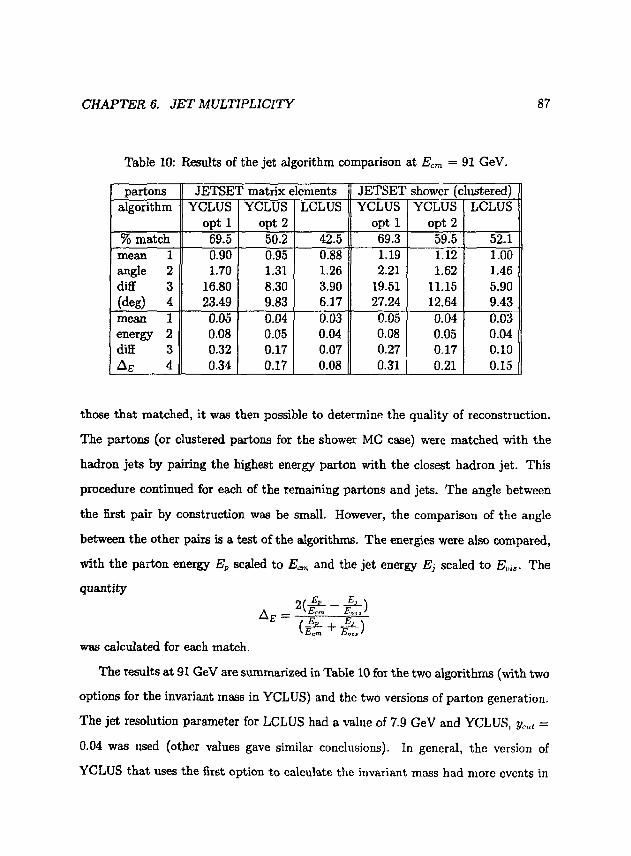
CHAPTER 6. JET MULTIPLICITY 87
Table 10: Results of the jet algorithm comparison at Ecm = 91 GeV.
partons JETSET matrix elements JETSET shower (clustered) algorithm YCLUS
opt 1 YCLUS
opt 2 LCLUS YCLUS
opt 1 YCLUS
opt 2 LCLUS
% match 69.5 50.2 42.5 69.3 59.5 52.1 mean 1 angle 2 diff 3 (deg) 4
0.90 1.70
16.80 23.49
0.95 1.31 8.30 9.83
0.88 1.26 3.90 6.17
1.19 2.21
19.51 27.24
1.12 1.62
11.15 12.64
1.00 1.46 5.90 9.43
mean 1 energy 2 diff 3 AE 4
0.05 0.08 0.32 0.34
0.04 0.05 0.17 0.17
0.03 0.04 0.07 0.08
0.05 0.08 0.27 0.31
0.04 0.05 0.17 0.21
0.03 0.04 0.10 0.15
those that matched, it was then possible to determine the quality of reconstruction.
The partons (or clustered partons for the shower MC case) were matched with the
hadron jets by pairing the highest energy parton with the closest hadron jet. This
procedure continued for each of the remaining partons and jets. The angle between
the first pair by construction was be small. However, the comparison of the angle
between the other pairs is a test of the algorithms. The energies were also compared,
with the parton energy Ep scaled to Ecm and the jet energy Ej scaled to £?„,•<,. The
quantity
was calculated for each match.
The results at 91 GeV are summarized in Table 10 for the two algorithms (with two
options for the invariant mass in YCLUS) and the two versions of parton generation.
The jet resolution parameter for LCLUS had a value of 7.9 GeV and YCLUS, ycut =
0.04 was used (other values gave similar conclusions). In general, the version of
YCLUS that uses the first option to calculate the invariant mass had more events in

CHAPTER 6. JET MULTIPLICITY 88
Table 11: Comparison of the two algorithms as Ecm is changed.
YCLUS option 2 LCLUS Ec,n
% match f3 {partem)/f3 (hadron) % match f3 (parton)/f3 (hadron) "•join
29 45.1 0.96 38.8 1.24 2.5 40 52.9 1.03 46.9 1.34 3.5 50 53.9 1.09 48.7 1.37 4.3 60 54.2 1.17 32.4 1.47 5.2 70 56.7 1.18 50.5 1.52 6.0 80 56.7 1.34 50.9 1.80 6.9 91 59.5 1.37 52.1 1.85 7.9 100 62.4 1.40 54.5 1.84 8.6
which the number of jets and partons match. However, the angle and energy of the
reconstructed hadron jets differed considerably from the partons. This option will
not be considered further.
The other two algorithms tested, YCLUS with the second option and LCLUS,
gave very similar results. They differed in that the first gave more eveuts where the
number of jets and partous matched and the second had a slightly better quality
of reconstruction. The next quality factor, namely the quality of the parton-hadron
match as the energy changes, was examined. For this study, the JETSET shower MC
was run for a range of energies, then the partons were clustered with ycut — 0.015
(other values gave the same results). At each energy, the events with the number of
hadron jets equal to the number of clustered partons were counted. Also, the ratio of
3-parton events to 3-hadron jet events was calculated. The results are in Table 11,
and show that the YCLUS algorithm produces a higher percentage of events with
equal numbers of jets as well as a smaller variation in the ratio. Therefore, as the
quality of the match is not too dissimilar, this form of the algorithm was chosen for
the jet analysis.

CHAPTER 6. JET MULTIPLICITY 89
JETSET 6.3 Shower BIGWIG 4.1
0.2 'cut
Figure 34: Jet fractions as a function of ycut- The solid line is from the JETSEIT 6.3 model, the dashed line from BIGWIG 4.1.
6.2 Je t Fractions
The goal is to measure the number of n-jet events and compare the results with the
model predictions. Define
_ number of n—jet events _ total number of events
as the jet fractions. For each value of ymti the uncorrected values of f\ to / 5 were
determined. Corrections for detector acceptance, initial state radiation and event
cuts were extracted from the MC simulation. The corrected values are in Figure 34.
The solid line is the JETSET shower model and the dashed line is the BIGWIG 4.1
model. Each set of points at a given ymt value uses all of the events, so the different

CHAPTER 6. JET MULTIPLICITY 90
0.4
0.3
CO 0.2
0.1
0 0 40 80
Figure 35: The 3-jet fraction VB Ecm.
Vcut points are not statistically independent. For a given value of j / ^ , , it can be seen
that both models are within 2a of the data, with the JETSET shower model being
closer. At a typical y^t value of 0.04, we have 60% 2-jet events, 37% 3-jet events
and 3% 4-jet events.
It is also interesting to see the variation with Ecm of the jet fractions. The variable
fz is chosen because, in first order, the number of 3-jet events is proportional to
a,. The coupling constant is expected to decrease with an increase in Ecm, so fs
is expected to decrease as well. Figure 35 shows f3 vs Ecm for several experiments
with the jet resolution parameter at j / r a t = 0.08 [69], along with the results with the
JETSET shower prediction. With the large error it is difficult to confirm that the
values are still decreasing, but the data is consistent with that expectation.
D Tasso • AMY • Jade • MarkU
JETSET 6.3 Shower

CHAPTER 6. JET MULTIPLICITY 91
4-90 y 6S30A9
Figure 36: Corrected differential jet distribution Di(y).
6.3 Differential Distribution
Another way of displaying the information about 3-jet events is to take the derivative
of the f3 distribution in Figure 34. Rather than measuring the fraction at a fixed ycui,
the value of y at which the event transforms from a 3-jet event to a 2-jet event is
found. Or equivalently, the minimum invariant mass of the 3 possible combinations of
the 3 jets is found. The advantage to this method of looking at, jets is that each event
enters only once into the distribution and therefore analyses of the match between
data and the models is more straightforward.
The function D2(y) is defined to be the distribution of y values for which the
events go from 3 - to 2-jet. The data values are shown in Figure 36 along with the
models. Again, the models predict the behaviour of the data.

Chapter 7
Inclusive Charged Track
Distributions
This chapter concentrates on the information given by the charged tracks in the event.
Examining the multiplicity, the momenta and the flow of the momenta in the event
gives clues about the mechanism that takes the partons to the detected hadrons. The
data in the first three sections has been previously published [70].
7.1 Charged Multiplicity
One of the obvious measurements to make about a group of events is to measure the
average number of charged particles produced. A mean charged-particle multiplicity
that has been corrected for detector effects was measured from the hadronic event
sample.
92

CHAPTER 7. INCLUSIVE CHARGED TRACK DISTRIBUTIONS 93
7.1.1 C o r r e c t i o n s
Most of the charged particles produced in an event at this Ecm have momenta below
1 GeV/c (see section 7.2). Unfortunately, these particles are also the most susceptible
to being scattered by the material in the detector, which means the tracks are more
difficult to reconstruct. In addition, tracks of all momenta are simply not seen if the
particle exits the ends of the detector. Due to these and other reasons, it was not
possible to use the bin-by-bin corrections described in section 4.6 as the correlation
between bins is large. For example, over 50% of Z° decays with 20 charged particles
produced will only have 11-16 charged particles measured.
The correction method used to obtain the mean charged-particle multiplicity was
an unfolding technique [61]. A distribution of observed multiplicities was measured
which must be corrected back to the original produced charged-particle multiplicity
distribution. One choice that must be made is how to correct for secondary decays
of the produced hadrons. For example, a B meson can decay within a few hundred
microns of the IP to several charged particles; the choice is whether to count the B or
the decay products. A standard technique is to let particles with lifetimes less than
3 x 10" l o s decay; others are assumed stable. The charged particles from all K% and
A decays were included.
The effects of the detector are modelled by a Monte Carlo simulation; this program
was used to produce a transition matrix A to give the probabilities for detecting
ridet charged particles if ngen are generated. Due to the low statistics of the data
sample, several multiplicities were grouped into one entry in the column vector D
(for detected) and another grouping was used for G (the generated multiplicity).
Therefore in general, A is not a square matrix.

CHAPTER 7. INCLUSIVE CHARGED TRACK DISTRIBUTIONS 94
Following a lc=<st squares technique [71], a x2 variable was defined:
where t runs over the detected bins, j runs over the generated bins and <r, is the
error on the detected bin. The solution involved finding the column vector G that
minimized the x2- Using matrix motation, a diagonal weight matrix W was defined,
with Wu = 1/of. Then
X2 = (AG - D)TW(AG - D).
The solution was
G = VATWD
with the covariance matrix V defined as:
V = ^WA)-1.
The uncorrected data distribution (grouped) and the result of the unfold are
in Figure 37. As the shape information in the corrected distribution is minimal,
the detected distribution is compared with the various MC models after detector
simulation. One can see that the models systematically overestimate the detected
multiplicity.
To calculatvs the mean of the corrected distribution, it is necessary know the value
at the center of each bin, &,-. The MC model was used to estimate that number. Then
if g, is the corrected number of entries in each bin,
^ E.6.& < nch >= — .

CHAPTER 7. INCLUSIVE CHARGED TRACK DISTRIBUTIONS 95
0.15
- ^ 0.1J
C, 0.05
r | • • •i 1 i 1 i 1 i i ' i i i i • Mark II Data • Mark II Da1a
- — JETSET 6.3 Shower -
" { — BIGWIG 4.1
(a) - (b) _
I. -
7
1 11
• f • " . . 1 j—i—r^»fc»J»«u«
11
• f • " 10 20 30 40
Detected n c h
10 20 30 Corrected n c h
40
Figure 37: Multiplicity distributions. The uncorrected data is shown in (a), along with the models after detector simulation. The result of the unfold is shown in (b).
7.1.2 Error calculation
The unfold procedure has both a statistical error and a systematic error associated
with it. The statistical error was calculated from
«r2 = GTVG
and had a value of 1.0. The systematic error from the unfold was generated by
grouping the multiplicities in different ways and by using different models to generate
the transition matrix A. The resulting spread in the corrected mean gave a systematic
error estimate of 0.4. In addition, there was an additional error of 0.8 multiplicity
units from uncertainties in the drift chamber efficiency simulation. The final result
for the mean corrected charge multiplicity was
< nch >= 19.0 ± l.O(stat) ± 0.9(sys).

CHAPTER 7. INCLUSIVE CHARGED TRACK DISTRIBUTIONS 96
As a check of this method, a corrected mean was calculated by making a simple
overall correction. The mean of the detected data distribution was 13.81 ±0.25 (stat).
From the MC simulation, the generated mean is 21.25 ± 0.07 and the detected mean
is 14.65 ± 0.06. Using the formula
. / < nch >gen\ < nch >cor=< Tick >det [— T I i
N < nch >det ' MC the corrected mean charged multiplicity was calculated to be
< nck > c o r = 20.03±0.36{stat)
which confirms the above number. The statistical error from the unfold procedure is
higher because the information is spread over more bins.
7.1.3 Variation w i th Ecm
Figure 38 shows the variation of mean charged multiplicity versus center-of-mass
energy from e + e~ experiments [24,61,72,73]. The solid line in the figure is from the
JETSET 6.3 shower model. Note that some experiments did not publish a systematic
error for their measurement. In those cases only the statistical error is plotted (most
errors are smaller than the symbol). The mean charged-particle multiplicity is growing
rapidly with Ecm and the value at 91 GeV is consistent with the model '.
7.2 Scaled Momentum
Another interesting property to measure is the momentum of the charged particles.
The maximum value possible for a particle to have is Ebeam- Each hadron would 1 Several different parameterizations of the energy variation have been proposed in the literature
(see e.g. [73]) but no fits were made as the large error precludes a precise determination of the fit parameters.

CHAPTER 7. INCLUSIVE CHARGED TRACK DISTRIBUTIONS 97
1 I I I II11 ' T " 1 1 1 1 1111 _ • Adone _
A Markl / - a LENA /<r
+ CLEO /
x PLUTO Jf - v HRS A
• TASSO IT " o JADE i"
A AMY • Markl
n
i i i i M i l 1 1 1 1 1 1 1 ll
10 50 100 2-90 • c m (GeV) 6S27A1
Figure 38: The corrected mean charged-particle multiplicity versus Em as measured by e + e" experiments. The solid line is the JETSET 6.3 shower model.

CHAPTER 7. INCLUSIVE CHARGED TRACK DISTRIBUTIONS 98
have that value if only two partons were produced and then they decayed to only one
hadron each. The scaled momentum x is defined for charged particles as x = 2 |p | /£ c m .
In theory, x has a range of 0 to 1. In practise, the data sample had very few particles
with large x.
Without the presence of gluon radiation, the principle of scaling predicts that the
distribution 1/<T dajdx should be the same for all values of Eon. With gluon radiation,
the amount of momentum available to the particles from each parton decreases. As
the center-of-mass energy increases, a higher number of partons are created and the
energy is shared between more particles. Thus the production of high x particles will
decrease.
7.2.1 Results
The raw distribution was corrected using the bin-by-bin technique. The correction
factors (in Table 12) are very uniform for all but the first bin, which represent particles
with momenta below 1 GeV. As mentioned in the previous section, these tracks are
subject to large errors in reconstruction. The corrected distribution 1/CT dajdx is in
Figure 39, compared with the results of the two QCD models. The normalization is
such that the integral of the curve yields the mean charged multiplicity. The models
agree well with the data.
7.2.2 Variation with Eon
To search for evidence of scaling violation, the distribution was divided into bins
in x and compared with similar values from other e+e~ annihilation experiments
[24,61,62]. The result is in Figure 40. The solid line in the figure represents the
JETSET shower model. The smallest x bin shows a strong rise with Em due to

CHAPTER 7. INCLUSIVE CHARGED TRACK DISTRIBUTIONS 99
Table 12: Correction factors for the charged particle inclusive distributions.
Bin X
range factor P±in
range factor Plout
range factor y
range factor 1 2 3 4 5 6 7 8 9 10 11 12 13
0.00-0.04 1.56 0.04-0.08 1-25 0.08-0.12 1.25 0.12-0.16 1.24 0.16-0.20 1.22 0.20-0.30 1.32 0.30-0.40 1.35 0.40-0.50 1.22 0.50-0.60 1.20 0.60-0.80 1.01
0.00-0.20 1.73 0.20-0.40 1.37 0.40-0.60 1.26 0.60-0.80 1.25 0.80-1.00 1.26 1.00-1.50 1.26 1.50-2.00 1.25 2.00-2.50 1.31 2.50-3.00 1.30 3.00-4.00 1.35 4.00-5.00 1.53 5.00-7.00 1.61 7.00-9.00 1.44
0.00-0.20 1.60 0.20-0.40 1.33 0.4C-0.60 1.24 0.60-0.80 1.24 0.80-1.00 1.25 1.00-1.50 1.33 1.50-2.00 1.41 2.00-2.50 1.38 2.50-3.00 1.21
0.0-0.5 2.47 0.5-1.0 1.88 1.0-1.5 1.49 1.5-2.0 1.25 2.0-2.5 1.20 2.5-3.0 1.20 3.0-3.5 1.19 3.5-4.0 1.20 4.0-4.5 1.09 4.5-5.0 0.79
x=2p/EC l
Figure 39: Corrected l/a dcr/dx distribution.

CHAPTER 7. INCLUSIVE CHARGED TRACK DISTRIBUTIONS 100
•a
O •o (0
10'
10 1
10°
10 M E-
10
i i r
•2 10
• Mark I I • TASSO A AMY
1 —
0.02<x<0.05
0.05<x<0.10
0.10<x<0.20
«-0.20<x<0.30 0.30<x<0.40 0.40<x<0.50
0.50<x<0.60
0.60<x<0.80 =
j i i u i. 30 50 100
cm (GeV) 300
Figure 40: l/<7 dtr/dx for a given x for various Ecm values. The solid line is from the JETSET 6.3 shower model.
CHAPTER 7. INCLUSIVE CHARGED TRACK DISTRIBUTIONS 101
the increased energy available to produce soft particles. At the higher x range, the
data points do show a scale breaking at a level that is consistent with the model
predictions.
7.3 Transverse Momentum
As well as the absolute value of a charged particle's momentum, the direction of the
particle also contains information. The sphericity axes described in Chapter 5 are
used to define a coordinate system for an event. In general, two axes define a plane
that contains most of the momentum of the event; the third axis is defined to make
an orthogonal system. Individual track directions with respect to these axes were
examined.
7.3.1 Variables
For each track, the components of momentum that are transverse to the sphericity
axis were examined; the first lay in the event plane (px,n) and the second lay out
of the event plane (pj.Dm). As discussed in the chapter on event shapes, most of
the events were planar. Therefore, the amount of transverse momentum out of the
event plane given to an individual particle measures the effects of the fragmentation
process. The fragmentation effect is also present for the transverse momentum in the
event plane, but is overshadowed by gluon radiation. The sphericity axis usually lies
along the direction of the most energetic quark and the gluon will have some p± with
respect to that axis that is passed on to the fragmentation products. As the energy
scale of the fragmentation is on the order of 1 GeV and gluons have energies up to «
30 GeV (at Erm = 91 GeV), the pL given by gluon radiation dominates.

CHAPTER 7. INCLUSIVE CHARGED TRACK DISTRIBUTIONS 102
> O 101
cT 10
10-1 r
10-'
r JETSET Shower 6.3 '-\ BIGWIG 4.1 -r\ • Markn 91 GeV -=
•rm
~
i II
IIII
J i
(a) 1
IIH
II|
iiin
il
„: I , I . -
„: I , I i S . i
0 .,
p l i n (GeV/c)
T T — JETSET Shower 6.3 :
- BIGWIG 4.1 • Markn 91 GeV
(b) i
Plout < G e V / c >
Figure 41: Distributions of transverse momenta (a) p^n and (b) p±mf
The fragmentation effects are expected to change very slowly with changes in Ecm-
On the other band, the energy available for gluon radiation increases rapidly and so
the px in the event plane is expected to increase almost linearly. (The small decrease
in the coupling constant as is a slight restraint on this effect.)
7-3.2 Results
The distributions were corrected in each bin and the result is shown in Figure 41 for
the two variables. There is generally very little momentum out of the event plane,
another indication that the sample consists of mostly 2- and 3-jet events. Again,
the distributions are normalized to the number of hadronic events and the integrals
are equal to the mean charged multiplicity. The error bars include statistical and
systematic uncertainties, where the main systematic error came from variations in
the correction factors from the models.

CHAPTER 7. INCLUSIVE CHARGED TRACK DISTRIBUTIONS 103
20 40 60 80 100 ECm (GeV)
Figure 42: Mean of the squared transverse momentum distribution versus Ecm.
7.3.3 Variation with Em
To be able to compare with other experiments, the mean of the squared transverse
momentum distributions, <pj.,„ 2 > and <p±But2 >, were calculated. The values are
0.70 ± 0.04 ± 0.03 and 0.121 ± 0.004 ± 0.003, where the first error is statistical and
the second systematic. The contributions to the systematic error for both cases were
from model differences in the correction factors and variations when the pxy cut was
changed. In addition, the distributions both had trackf at high p\ that contributed
substantially to the mean. The weight of these tracks was varied to estimate another
contribution to the systematic error.
These values, along with those from other experiments [24,61,62,64], are plotted
in Figure 42. The solid line is the JETSET shower model result. As expected, the
<P±o»t2 > shows only a small increase as Ecm increases. The transverse momentum

CHAPTER 7. INCLUSIVE CHARGED TRACK DISTRIBUTIONS 104
in the event plane does increase significantly. The prediction of the JETSET shower
model is 2cr below what is observed. However, this is not a significant inadequacy
of the models. It may be possible to find a parameter set that would give a result
consistent with both the 91 GeV and the 29 GeV data values.
7.4 Rapidity
Again the particle's momentum with respect to the overall momentum flow in the
event is used to give information. For this variable the thrust axes are used to define
a coordinate system.
7.4.1 Variable definition
For each charged track, the rapidity y is defined as
y- i l n £ + a 2 E - n
where E is the particle energy and p\\ the component of momentum along the thrust
axis. For all particles, the energy is calculated assuming a pion mass. The rapidity
distribution is characterized by a broad plateau with a dip near y = 0 and a steep
fall-off at high values. Changes in these characteristics with changes in Ecm are
predicted by QCD: the plateau is expected to increase in height (as the multiplicity
is increasing) and to broaden due to the increase in parton energy.
7.4.2 Results
The observed distribution was corrected using the bin-by-bin factors shown in Ta
ble 12. The result is shown in Figure 43 with the QCD models. We do see a slight

CHAPTER 7. INCLUSIVE CHARGED TRACK DISTRIBUTIONS 105
Figure 43: Corrected rapidity distribution.
dip at y = 0 and the broad plateau. The JETSET shower model overestimates the
height of the plateau; this is associated with the difference in the charged multiplicities
seen in section 7.1.

Chapter 8
Conclusions
Several of the distributions which characterize the hadronic decays of the Z° boson
have been measured from the initial Mark II data sample. The shape distributions
and the jet rates show that a majority of the events are 2-jet events, assumed to
result from the decay of a Z° boson into a quark and an anti-quark. Some of the
events, however, have a significant amount of momentum away from a single axis.
The parton structure of these events is most likely qqg, where the energetic gluon has
been radiated from one of the quarks.
All measured quantities were corrected for detector effects and were compared
with the predictions of two QCD-based Monte Carlo models. Both JETSET version
6.3 and BIGWIG 4.1 used parton shower generation for the perturbative region; the
model for the fragmentation region was different. The model parameters were tuned
at 29 GeV with the Mark II data from PEP. In all cases both models predicted
distributions that were in agreement with the data distributions measured at Ecm =
91 GeV.
The shape distributions that were measured were sphericity (S), thrust (1-T),
106

CHAPTER 8. CONCLUSIONS 107
aplanarity (A), and the scaled invariant masses M£/s and (Mf;/s — Mf js). They
each highlight different aspects of the events. The thrust is a good measure of the
2-jet events, whereas aplanarity is sensitive to 4-jet events and fragmentation effects.
The mean values of each of these distributions were also compared to those from
e + e~ experiments at lower center-of-mass energies. The variation with Ecm shows
that the events have a higher proportion of tightly collimated 2-jet events.
A study of two commonly used jeJ fading algorithms was performed. It wat> f 1
that the YCLUS rdgorithm, first used by the JADE experiment, reconstructed the
quark directions and energies nearly as well as the LCLUS algorithm which is included
in the JETSET model software. However, YCLUS showed a more consistent result
with a changing center-of-mass energy and more events had the same number of
reconstructed jets as initial partons. Using- the YCLUS algorithm, the number of jets
as a function of the jet resolution parameter ycut was calculated. At a typical ycut
value of 0.04, there are 60% 2-jet events, 27% 3-jet events, and 3% 4-j«'t events. Also
shown was the fraction of 3-jet events versus center-of-mass energy. The statistical
error is too large to make any statement about the running of as.
Charged-particle inclusive distributions were also measured. An unfolding tech
nique was used to obtain a corrected mean charged multiplitiy of < nch > = 19.0 ±
1.0(stat) ± Q.9(sys). The scaled momentum distribution, when compared with lower
energy e+e~ annihilation data, showed slight scaling violations. The transverse mo
menta in and out of the event pla^a were calculated u^mg the sphericity axes as the
coordinate system. The mean values of the transverse momenta squared distribu
tions were compared with values from lower Ecm experiments. The <pj.,„ 2 > showed
a rapid rise, indicating that harder gluons are being radiated in the event plane. The
< P±out2 > grew at a much slower rate, showing that the fragmentation effects are

CHAPTER 8. CONCLUSIONS 108
not very energy-dependent. The last distribution measured was the rapidity y of the
charged tracks. The data distribution has the expected characteristics.

Bibliography
[1] S. Weinberg, Phys. Rev. Lett. 19 (1967) 1264.
[2] G. Arnison et al., Phys. Lett. B126 (1983) 398.
[3] P. Bagnaia et al., Phys. Lett. B129 (1983) 130.
[4] G. S. Abrams et ai, Pbys. Rev. Lett. 63 (1989) 724.
[5] D. Decamp et al. (ALEPH), Phys. Lett. B231 (1989) 519.
P. Aamio et al. (DELPHI), Phys. Lett. B231 (1989) 539.
B. Adeva et al. (L3), Phys. Lett. B231 (1989) 509.
M. Z. Akrawy et al. (OPAL), Phys. Lett. B231 (1989) 530.
[6] G. Peldman ed., Proceedings of the Second Mark II Workshop on SLC Physics,
SLAC-Report-306, November, 1986.
G. Feldman ed., Proceedings of the Third Mark II Workshop on SLC Physics,
SLAC-Report-315, July, 1987.
J. Ellis and R. Peccei eds., Physics at LEP, Vols 1 and 2, CERN 86-02, 21 Feb.
1986.
109

BIBLIOGRAPHY 110
[7] F. Halzen and A. D. Martin, Quarks and Leptons, J. Wiley and Sons (1984).
D. H. Perkins, Introduction to High Energy Physics, Addison-Wesley (1987).
[8] S. L. Glashow, Nucl. Phys. 22 (1961) 579.
[9] A. Salam, 8 t h Nobel Symposium, N. Svartholm ed., Almquist and Wiksell, Stock
holm (1968) 367.
[10] G. S. Abrams et al, Phys. Rev. Lett. 63 (1989) 2173.
[11] A. Barbaro-Galtieri, 8 t h Workshop on pp Collider Physics, LBL—28673, Feb.
1990. Recent limits of mt > 89 GeV have also been reported but are not yet
published.
[12] D. J. Gross and F. Wilczek, Phys. Rev. Lett. 30 (1973) 1343.
H. D. Politzer, Phys. Rev. Lett. 30 (1973) 1346.
[13] S. Komamiya et al., Phys. Rev. Lett. 64 (1990) 987.
[14] P. Hoyer et al., Nucl. Phys. B161 (1979) 349.
A. Ah et al, Phys. Lett. 93B (1980) 155.
[15] W. Bartel et al. (JADE), Z. Phys. C21 (1983) 37.
W. Bartel et al. (JADE), Phys. Lett. B134 (1984) 275.
W. Bartel et al. (JADE), Phys. Lett. B157 (1985) 340.
H. Aihara et al. (TPC), Z. Phys. C28 (1985) 31.
M. Althoff et al. (TASSO), Z. Phys. C29 (1985) 29.
H. Aihara et al. (TPC), Phys. Rev. Lett. 57 (1986) 945.
P. Sheldon et al. (Mark II), Phys. Rev. Lett. 57 (1986) 1398.
[16] G. Ballochi and R. Odorico, CERN-EP/89-162, Dec, 1989.

BIBLIOGRAPHY 111
[17] B. Andersson et al., Phys. Rep. 97 (1983) 31.
X. Artni, Phys. Rep. 97 (1987) 1.
A. Casher, H. Neuberger, and S. Nussinov, Phys. Rev. D20 (1979) 179.
A. Casher, H. Neuberger, and S. Nussinov, Phys. Rev. D21 (1980) 1966.
[18] T. Sjostrand, Status of Fragmentation Models, Int. J. Mod. Phys. A3 (1988) 751.
B. Bambah et al., QCD Generators at LEP, CERN-TH-5466/89. July 1989.
[19] G. Marchesini and B. R. Webber, Nucl. Phys. B238 (1984) 1.
B. R. Webber, Nucl. Phys. B238 (1984) 492.
[20] G. Altarelli and G. Parisi, Nucl. Phys. B216 (1977) 298.
[21] W. Hofmann, in Proceedings of International Symposium on Lepton and Photon
Interactions at High Energies, Hamburg, Germany (1987).
[22] T. Sjostrand, Comput. Phys. Commun. 39 (1986) 347.
T. Sjostrand and M. Bengtsson, Comput. Phys. Commun. 43 (1987) 367.
M. Bengtsson and T. Sjostrand, Nucl. Phys. B289 (1987) 810.
[23] F. Gutbrod, G. Kramer and G. Schiergolz, Z. Phys. C21 (1984) 235.
[24] A. Petersen et al., Phys. Rev. D37 (1988) 1.
[25] W. Braunschweig et al., 1. Phys. C41 (1988) 359.
[26] B. Richter et al, SLAC-PUB-4367, 1987 Lepton and Photon Symposium.
SLAC-229, Conceptual SLC Design Report, June 1980.
[27] W. Farr et al., Nucl. Instr. and Meth. 156 (1978) 283.
[28] G. Hanson, Nucl. Instr. and Meth. A252 (1983) 343.

BIBLIOGRAPHY 112
[29] D. Briggs et al., IEEE Trans. Nucl. Sci. NS-32 (1985) 653.
[30] D. Bernstein et al., IEEE Trans. Nucl. Sci. NS-33 (1986) 86.
[31] H. Bratman et al., IEEE Trans. Nucl. Sci. NS-32 (1985) 336.
[32] J. Perl et al., Nucl. Instr. and Meth. A252 (1986) 616.
[33] J. Va'Vra et al., Nucl. Instr. and Meth. 203 (1982) 109.
[34) G. S. Abrams et al., Nucl. Instr. and Meth. A281 (1989) 55.
[35] G. S. Abrams et al, IEEE Trans. Nucl. Sci. NS-25 (1978) 309.
G. S. Abrams ei al, IEEE Trans. Nucl. Sci. NS-27 (1980) 59.
[36] W. J. Willis and V. Radeka, Nucl. Instr. and Meth. 120 (1974) 221.
[37] E. Cisneros et al., IEEE Trans. Nucl. Sci. NS-24 (1977) 413.
[38] M. Breidenbach et al., IEEE Trans. Nucl. Sci. NS-25 (1978) 706.
[39] R. L. Ford and W. R. Nelson, EGS3, SLAC-210, June 1978.
[40] M. Nelson et al., Phys. Rev. Lett. 50 (1983) 1542.
[41] M. E. Nelson, Ph.D. Thesis, LBL-16724mc, October 1983.
D. A. Karlen, Ph.D. Thesis, SLAC-325, March 1988.
[42] J. A. Kadyk, Proceedings of the Gas Sampling Calorimetry Workshop II,
Batavia, IL, (1985) 373.
[43] R. C. Jared et al., IEEE Trans. Nucl. Sci. NS-33 (1986) 916.
[44] J. Haggerty, Mark II/SLC Note #137 (1986), unpublished.

BIBLIOGRAPHY 113
[45] H. Brafman et al, SLAC-PUB-2033, October 1977.
[46] T. Himel, SLAC-REP-223, October 1979.
[47] J. E. Grund, IEEE Trans. Nucl. Sci. NS-26 (1979) 220.
[48] R. Aleksan et al., SLAC-PUB-4636, May 1988.
[49] Mark II Collaboration and SLC Final Focus Group, SLAC-SLC-PROP-2, April
1986.
[50] M. E. Levi et al., Nucl. Instr. Meth. A281 (1989) 265.
[51] Iron-Nickel alloy with low thermal expansion coefficient.
[52] J. Seeman et al., SLAC-PUB-3945, April 1986, published in proceedings
LINAC86, 441.
[53] D. J. Nelson et al., IEEE Trans. Nucl. Sci. NS-28 (1981) 336.
[54] J. E. Gnind, IEEE Trans. Nucl. Sci. NS-27 (1980) 599.
J. S. Brown et al., Nucl. Instr. and Meth. 221 (1984) 503.
[55] E. J. Siskind, IEEE Trans. Nucl. Sci. NS-30 (1983) 188.
[56] A. J. Lankford and T. Glanzman, IEEE Trans. Nucl. Sci. NS-31 (1984) 225.
T. Barklow et al., IEEE Trans. Nucl. Sci. NS-33 (1986) 775.
[57] J. D. Bjorken and S. J. Brodsky, Phys. Rev. Dl (1970) 1416.
G. Hanson et al., Phys. Rev. Lett. 35 (1975) 1609.
[58] E. Farhi, Phys. Rev. Lett. 39 (1977) 1587.
R. Brandelik et al., Phys. Lett. B86 (1979) 243.

BIBLIOGRAPHY 114
[59] G. S. Abrams et al, Phys. Rev. Lett. 63 (1989) 1558.
[60] Ch. Berger et al. (Pluto), Z. Phys. C12 (1982) 297.
H. J. Behrend et al. (CELLO), Z. Phys. C44 (1989) 63.
[61] M. Althoff et al. (TASSO), Z. Phys. C22 (1984) 307.
[62] Y. K. Li et al. (AMY), KEK Preprint 89-149, Nov. 1989.
[63] W. Braunschweig et al. (TASSO), Z. Phys. C41 (1988) 63.
[64] D. Bender et al. (HRS), Phys. Rev. D31 (1985) 1.
[65] G. S. Abrams et al., Phys. Rev. Lett. 63 (1989) 2447.
C. K. Jung et al., Phys. Rev. Lett. 64 (1990) 1091.
M. Swartz et al., SLAC-PUB-5176, Submitted to Phys. Rev. Lett.
P. R. Burchat et ai., SLAC-PUB-5172, Submitted to Pays. Rev. Lett.
S. Komamiya et al., SLAC-PUB-5175, Submitted to Phys. Rev. Lett.
[66] R. Brandelik et al. (TASSO), Phys. Lett. B86 (1979) 243.
Ch. Berger et al. (Pluto), Phys. Lett. B86 (1979) 418.
D. P. Barber et al. (Mark J), Phys. Rev. Lett. 43 (1979) 830.
W. Bartel et al. (JADE), Phys. Lett. B91 (1980) 142.
[67] T. Sjostrand, Comput. Phys. Commun. 28 (1983) 227.
[68] W. Bartel et al. (JADE), Z. Phys. C33 (1986) 23.
S. Bethke, Habilitationschrift, University of Heidelberg (1987) (unpublished).
[69] S. Bethke et al. (JADE), Phys. Lett. B213 (1988) 235.
W. Braunschwieg et al. (TASSO), Phys. Lett. B214 (1988) 286.
I. H. Park et al. (AMY), Phys. Rev. Lett. 62 (1989) 1713.

BIBLIOGRAPHY 115
[70] G. S. Abrams et al., Phys. Rev. Lett. 64 (1990) 1334.
[71] V. Blobel, in Formulae and Methods in Experimental Data Evaluation, Vol. 3,
CERN (1984).
[72] C. Bacci et al. (Adone), Phys. Lett. B86 (1979) 234.
J. L. Siegrist et al. (Mark I), Phys. Rev. D26 (1982) 969.
B. Niczyporuk et al. (Lena), Z. Phys. C9 (1981) 1.
M. S. Alam et al. (Cleo), Phys. Lett. B49 (1982) 357.
Ch. Berger et al. (Pluto), Phys. Lett. B95 (1980) 313.
W. Bartel et al. (JADE), Z. Phys. C20 (1983) 187.
H. W. Zheng et al. (AMY), KEK-Preprint 90-5.
[73] M. Derrick et al. (HRS), Phys. Rev. D34 (1986) 3304.
Copyright © 2022 FDOKUMEN