arX

iv:1

012.

4098

v2 [

hep-

ph]

7 M

ar 2

011

SI-HEP-2010-19

Next-to-leading-order correction to pion form factor in kT factorization

Hsiang-nan Lia,b,c, Yue-Long Shena,d, Yu-Ming Wange,f , Hao ZoufaInstitute of Physics, Academia Sinica, Taipei, Taiwan 115, Republic of China

bDepartment of Physics, National Cheng-Kung University, Tainan, Taiwan 701, Republic of ChinacDepartment of Physics, National Tsing-Hua University, Hsinchu, Taiwan 300, Republic of China

dCollege of Information Science and Engineering,Ocean University of China, Qingdao, Shandong 266100, P.R. China

eTheoretische Physik 1, Fachbereich Physik, Universitat Siegen, D-57068 Siegen, Germanyf Institute of High Energy Physics and Theoretical Physics Centerfor Science Facilities, P.O. Box 918(4) Beijing 100049, China

We calculate next-to-leading-order (NLO) correction to the pion electromagnetic form factorat leading twist in the kT factorization theorem. Partons off-shell by k2

T are considered in bothquark diagrams and effective diagrams for the transverse-momentum-dependent (TMD) pion wavefunction. The light-cone singularities in the TMD pion wave function are regularized by rotatingthe Wilson lines away from the light cone. The soft divergences from gluon exchanges among initial-and final-state partons cancel exactly. We derive the infrared-finite kT -dependent NLO hard kernelfor the pion electromagnetic form factor by taking the difference of the above two sets of diagrams.Varying the renormalization and factorization scales, we find that the NLO correction is smaller,when both the scales are set to the invariant masses of internal particles: it becomes lower than 40%of the leading-order (LO) contribution for momentum transfer squared Q2 > 7 GeV2. It is observedthat the NLO leading-twist correction does not play an essential role in explaining the experimentaldata, but the LO higher-twist contribution does.

PACS numbers: 12.38.Bx, 12.38.Cy, 12.39.St

I. INTRODUCTION

The kT factorization theorem [1–6] in perturbative QCD (PQCD) has caught a lot of attention recently (see [7, 8]for its recent applications). How to derive a hard kernel beyond leading order (LO) in the kT factorization theoremis one of the important subjects. We have proposed the prescription that partons in both QCD quark diagrams andeffective diagrams for transverse-momentum-dependent (TMD) hadron wave functions are off mass shell by k2T [9].Since the gauge dependence cancels between the two sets of diagrams, their difference defines a gauge-invariant hardkernel. The gauge invariance of the kT factorization theorem has been investigated in [10, 11], and proved in [12].The light-cone singularities, appearing in the naive definition of TMD wave functions, are regularized by rotating theWilson lines away from the light cone [13–15]. Following the above prescription, the next-to-leading-order (NLO)correction to the pion transition form factor associated with the process πγ∗ → γ has been calculated at leading twist[11]. Both the large double logarithms αs ln

2 kT and αs ln2 x, x being a parton momentum fraction, were identified.

The former is absorbed into the pion wave function and summed to all orders in αs by the kT resummation, and thelatter is absorbed into a jet function and summed to all orders in αs by the threshold resummation.In this paper we shall extend the framework to the more complicated pion electromagnetic form factor associated

with the process πγ∗ → π. Our work represents the first NLO study of this quantity at leading twist in the kTfactorization theorem. The NLO correction to the pion form factor has been evaluated in the collinear factorizationtheorem by several groups [16–24]. For πγ∗ → π, not only the collinear divergences from gluon emissions collimatedto the initial- and final-state pions, but also the soft divergences from gluon exchanges between the two pions exist.Therefore, it is nontrivial to demonstrate that the collinear divergences in the quark diagrams are cancelled by those inthe pion wave functions, and the soft divergences cancel among themselves. The computation of the box and pentagondiagrams for the pion form factor is also technically involved. The renormalization scale µ and the factorization scaleµf are introduced by higher-order corrections to the quark diagrams and to the effective diagrams, respectively. Weshall show that the NLO correction to the pion form factor is smaller, when both the scales are set to the invariantmasses of internal particles as postulated in [5, 25]: it becomes lower than 40% of the LO contribution for momentumtransfer squared Q2 > 7 GeV2. The variation of the pion form factor with µ and µf gives an estimate of the theoreticaluncertainty in our analysis.Another related subject concerns the shape of the pion distribution amplitudes. It has been pointed out [26] that

the recent BaBar data of the pion transition form factor Fπγ(Q2) [27] at low (high) Q2 indicate an asymptotic (flat)

leading-twist, i.e., twist-2 pion distribution amplitude. However, a pion distribution amplitude ought to be universal.

2

These seemingly contradictory observations have been reconciled in the kT factorization theorem [26]: the increase ofthe measured Q2Fπγ(Q

2) for Q2 > 10 GeV2 was explained by convoluting a kT -dependent hard kernel with a flat pion

distribution amplitude. The low Q2 data were accommodated by including the threshold resummation of αs ln2 x,

which provides a strong suppression at the endpoints of x. The suppression becomes stronger as Q2 decreases. Thatis, the twist-2 pion distribution amplitude multiplied by the threshold resummation factor behaves like the asymptoticmodel at low Q2 effectively. In this work we shall show that the asymptotic models for both the twist-2 and two-partontwist-3 pion distribution amplitudes also lead to results in better agreement with the data of the pion form factor atlow Q2, compared to those from the non-asymptotic models. It is found that the NLO twist-2 correction does not playan essential role in accounting for the data, but the contribution from the LO two-parton twist-3 pion distributionamplitudes does, a conclusion the same as drawn in [28].In Sec. II we calculate the O(α2

s) QCD quark diagrams, the O(αs) effective diagrams for the TMD pion wave func-tion, and their convolution with the O(αs) hard kernel, considering partons off-shell by k2T . Since the kT factorizationtheorem is appropriate for QCD processes dominated by contributions from small x [9], we shall keep only termsin leading power of x. Taking the difference between the two sets of diagrams, we derive the NLO kT -dependenthard kernel for the pion form factor. Section III contains the numerical investigation, in which we obtain the partialcontributions to the pion form factor from different twists and orders, and the relative importance of the LO andNLO twist-2 contributions. We also examine the dependence of our results on the renormalization and factorizationscales, and on the shape of the pion distribution amplitudes. Section IV is the conclusion.

II. NLO CORRECTIONS

In this section we compute the O(α2s) quark diagrams in QCD and the O(αs) effective diagrams for the pion

wave function in the Feynman gauge, and then derive the NLO hard kernel for the pion electromagnetic form factorin the kT factorization theorem. The momentum P1 (P2) of the initial-state (final-state) pion is chosen as P1 =(P+

1 , 0,0T ) (P2 = (0, P−2 ,0T )). The anti-quark q carries the momentum k1 = (x1P

+1 , 0,k1T ) in the initial state and

k2 = (0, x2P−2 ,k2T ) in the final state, as indicated by the LO quark diagrams in Fig. 1. The parton virtuality k2T

regularizes the collinear and soft divergences into the logarithm ln k2T . We shall focus only on Fig. 1(a), since theNLO correction to Fig. 1(b) can be obtained from that to Fig. 1(a) by exchanging the kinematic variables of the twopions. The NLO corrections to the other two LO quark diagrams with the virtual photon attaching to the anti-quarkline are then obtained via the variable exchanges between the quark and the anti-quark. According to the hierarchyQ2 ≫ xQ2 ≫ k2T in the small-x region, we keep only those terms that do not vanish in the x → 0 and kT → 0 limit.Figure 1(a) leads to the amplitude

H(0)(x1, k1T , x2, k2T , Q2) = −g2CF

Nc

(√2Nc)2

Tr[γνγ5 6P2γν(6P2−6 k1)γµ 6P1γ5]

(P2 − k1)2(k1 − k2)2,

= g2CFTr(6P2 6P1γµ 6P1)

Q2(x1x2Q2 + |k1T − k2T |2), (1)

where Nc is the number of colors, CF is a color factor, 6P1γ5/√2Nc and γ5 6P2/

√2Nc are the twist-2 spin structures of

the initial- and final-state pions, respectively, and Q2 ≡ 2P1 · P2 is the momentum transfer squared from the virtualphoton. To reach the last line in Eq. (1), we have applied the hierarchy x1Q

2 ≫ k21T to the internal quark propagator.The denominator x1x2Q

2+ |k1T −k2T |2 comes from the virtuality of the LO hard gluon. The |k1T −k2T |2 term maynot be negligible compared to x1x2Q

2 in the small-x region, so it is retained.The NLO hard kernel H(1) is defined, in the kT factorization theorem, by [9]

H(1)(x1, k1T , x2, k2T , Q2) = G(1)(x1, k1T , x2, k2T , Q

2)

−∫

dx′1d

2k′1TΦ(1)(x1, k1T ;x

′1, k

′1T )H

(0)(x′1, k

′1T , x2, k2T , Q

2)

−∫

dx′2d

2k′2TH(0)(x1, k1T , x

′2, k

′2T , Q

2)Φ(1)(x2, k2T ;x′2, k

′2T ), (2)

where G(1) denotes the NLO quark diagrams associated with Fig. 1(a), and Φ(1) collects the O(αs) effective diagramsfor the twist-2 quark-level wave function [9, 29]

Φ(x1, k1T ;x′1, k

′1T ) =

∫

dy−

2π

d2yT(2π)2

e−ix′

1P+

1y−+ik′

1T ·yT 〈0|q(y)Wy(n)†In;y,0W0(n) 6 n−γ5q(0)|q(P1 − k1)q(k1)〉. (3)

3

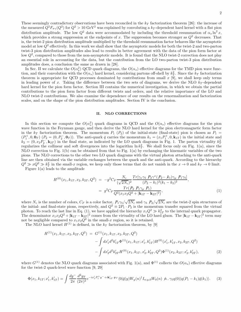
(a)k1

P1 − k1 P2 − k2

k2

(c) (d)

(b)

FIG. 1: Leading-order quark diagrams for πγ∗

→ π with ⊗ representing the virtual photon vertex.

In the above expression y = (0, y−,yT ) is the coordinate of the anti-quark field q, n− = (0, 1,0T ) is a null vectoralong P2, |q(P1 − k1)q(k1)〉 is the leading Fock state of the pion, and the Wilson line Wy(n) with n2 6= 0 is written as

Wy(n) = P exp

[

−ig

∫ ∞

0

dλn ·A(y + λn)

]

. (4)

The two Wilson lines Wy(n) and W0(n) are connected by a vertical link In;y,0 at infinity [30, 31]. Equation (3) willgenerate additional light-cone singularities from the region with a loop momentum collinear to n−, as the Wilson linedirection approaches the light cone, i.e., as n → n− [13]. That is, n2 serves as an infrared regulator for the light-conesingularities.

A. NLO Quark Diagrams

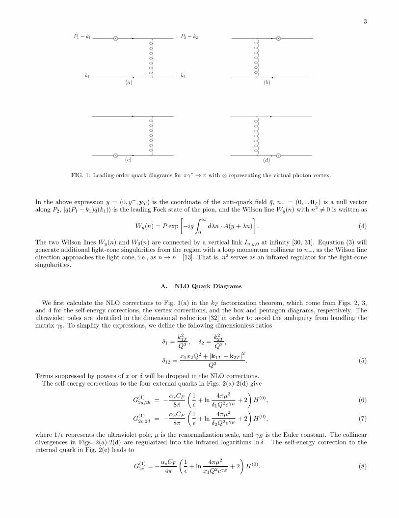
We first calculate the NLO corrections to Fig. 1(a) in the kT factorization theorem, which come from Figs. 2, 3,and 4 for the self-energy corrections, the vertex corrections, and the box and pentagon diagrams, respectively. Theultraviolet poles are identified in the dimensional reduction [32] in order to avoid the ambiguity from handling thematrix γ5. To simplify the expressions, we define the following dimensionless ratios

δ1 =k21TQ2

, δ2 =k22TQ2

,

δ12 =x1x2Q

2 + |k1T − k2T |2Q2

. (5)

Terms suppressed by powers of x or δ will be dropped in the NLO corrections.The self-energy corrections to the four external quarks in Figs. 2(a)-2(d) give

G(1)2a,2b = −αsCF

8π

(

1

ǫ+ ln

4πµ2

δ1Q2eγE

+ 2

)

H(0), (6)

G(1)2c,2d = −αsCF

8π

(

1

ǫ+ ln

4πµ2

δ2Q2eγE

+ 2

)

H(0), (7)

where 1/ǫ represents the ultraviolet pole, µ is the renormalization scale, and γE is the Euler constant. The collineardivergences in Figs. 2(a)-2(d) are regularized into the infrared logarithms ln δ. The self-energy correction to theinternal quark in Fig. 2(e) leads to

G(1)2e = −αsCF

4π

(

1

ǫ+ ln

4πµ2

x1Q2eγE

+ 2

)

H(0). (8)

4

(a) (b) (c)

(d) (e) (f)

(g) (h) (i)

FIG. 2: Self-energy diagrams.

(a) (b) (c)

(d) (e)

FIG. 3: Vertex-correction diagrams.

The ultraviolet poles in Eqs. (6) and (7) are half of that in Eq. (8), because an additional factor 1/2 is associated withan external particle. The internal quark is off-shell by the invariant mass squared x1Q

2, which replaces the argumentsk2T of the infrared logarithms in Eqs. (6) and (7). The self-energy correction to the hard gluon, summing the quark-,gluon- and ghost-loop contributions in Figs. 2(f)-2(i), is written as

G(1)2f+2g+2h+2i =

αs

4π

(

5

3Nc −

2

3Nf

)(

1

ǫ+ ln

4πµ2

δ12Q2eγE

)

H(0), (9)

with Nf being the number of quark flavors. In this case the logarithm depends on the invariant mass squared δ12Q2

of the hard gluon.The results from the five diagrams Figs. 3(a)-3(e) for the vertex corrections are summarized as

G(1)3a =

αsCF

4π

(

1

ǫ+ ln

4πµ2

Q2eγE

+ 2

)

H(0), (10)

G(1)3b = − αs

8πNc

(

1

ǫ+ ln

4πµ2

x1Q2eγE

+ 2 lnx1

δ2+

7

2

)

H(0), (11)

5

G(1)3c = − αs

8πNc

(

1

ǫ+ ln

4πµ2

δ12Q2eγE

− 2 lnδ12δ1

lnδ12δ2

+ 2 lnδ212δ1δ2

− 2π2

3+

11

2

)

H(0), (12)

G(1)3d =

αsNc

8π

(

3

ǫ+ 3 ln

4πµ2

δ12Q2eγE

+ 2 lnδ212δ1δ2

+23

2

)

H(0), (13)

G(1)3e =

αsNc

8π

[

3

ǫ+ 3 ln

4πµ2

x1Q2eγE

+ 2 lnx1

δ2

(

1− lnx1

δ12

)

+ lnx1

δ12− 2

3π2 +

7

2

]

H(0). (14)

The ultraviolet poles in the self-energy and vertex corrections are summed into

αs

4π

(

11− 2

3Nf

)

1

ǫ, (15)

for Nc = 3, which is the same as obtained in [22]. This pole term determines the renormalization-group (RG) evolutionof the coupling constant αs.

The loop correction G(1)3a to the photon vertex does not contain an infrared logarithm, because of the sequence of

the γ-matrices in the fermion flow. The correction G(1)3b to the upper gluon vertex contains only the infrared logarithm

associated with the final-state pion. The other end of the radiative gluon attaches to the internal quark line, so G(1)3b

depends on x1Q2, and does not generate a double logarithm. The correction to the lower gluon vertex in Fig. 3(c)

depends on the momentum transfer squared δ12Q2 from the LO hard gluon, and on the two infrared regulators δ1 and

δ2 from the incoming and outgoing partons. The expression of G(1)3c is symmetric under the exchange of δ1 and δ2 as

expected. The ln(δ12/δ1) ln(δ12/δ2) term is not a large double logarithm in the small-x region, where ln δ1 ln δ2 arisesfrom the soft region of the radiative gluon. It is obvious from the convolutions of Φ(1) and H(0) in Eq. (2) that thissoft logarithm can not be cancelled by the infrared logarithms in the effective diagrams: there is no chance for ln δ1associated with the initial-state pion and ln δ2 associated with the final-state pion to appear in a product. Therefore,cancellation must occur within this type of soft logarithms as demonstrated below.

The triple-gluon vertex correction G(1)3d also depends on the scale δ12Q

2, and contains the same infrared logarithm

ln(δ212/δ1δ2) as in G(1)3c but with different color factors. Their sum is proportional to CF : −1/Nc + Nc = 2CF ,

implying the factorization of this infrared logarithm in color flow. It is then possible that it will be cancelled by thecorresponding logarithm in the effective diagrams, whose color factor is also CF . This combination of quark diagramsfor achieving factorization also takes place elsewhere. Another triple-gluon vertex correction in Fig. 3(e) involves theinvariant masses squared of the virtual quark and of the hard gluon as shown in Eq. (14). At small x, the quark qin Fig. 3(e) is energetic, leading to the collinear logarithmic enhancement ln(x1/δ2), and the hard gluon has a smallinvariant mass, leading to the soft enhancement ln(x1/δ12). Their overlap then gives rise to the important double

logarithm ln(x1/δ2) ln(x1/δ12) in G(1)3e . This double logarithm can be reexpressed as

2 lnx1

δ2ln

x1

δ12= ln2

x1

δ2+ ln2

δ12x1

− ln2 δ12δ2

, (16)

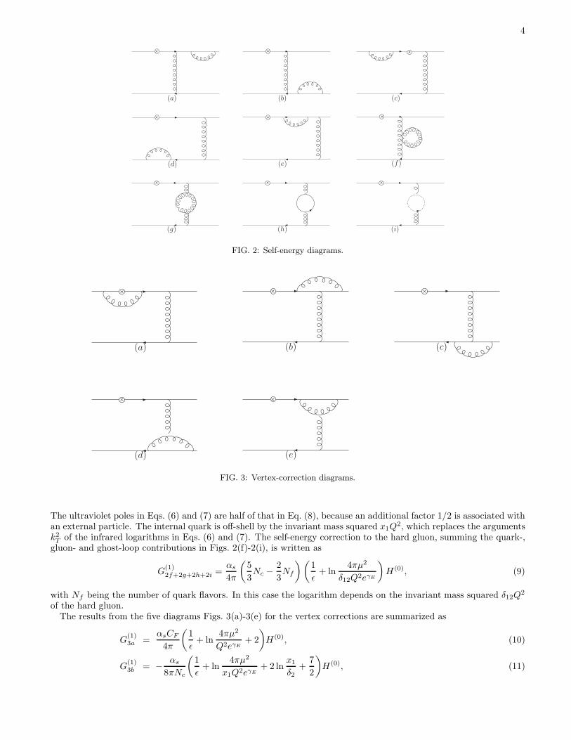
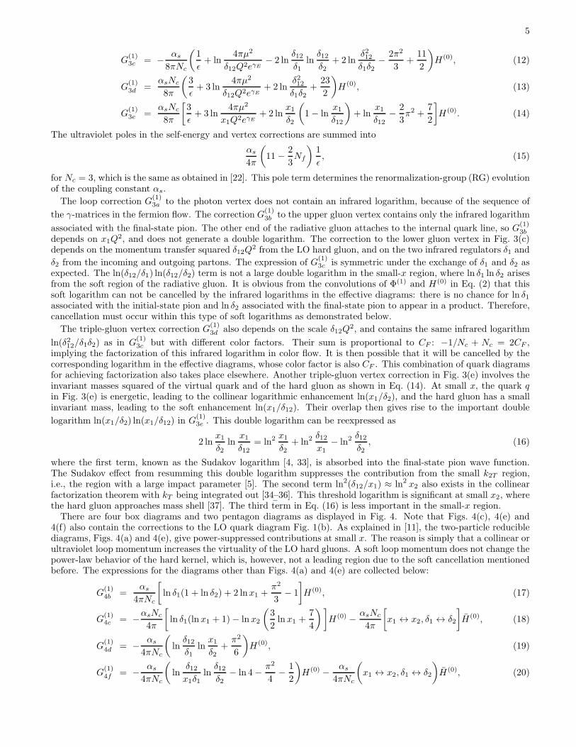
where the first term, known as the Sudakov logarithm [4, 33], is absorbed into the final-state pion wave function.The Sudakov effect from resumming this double logarithm suppresses the contribution from the small k2T region,i.e., the region with a large impact parameter [5]. The second term ln2(δ12/x1) ≈ ln2 x2 also exists in the collinearfactorization theorem with kT being integrated out [34–36]. This threshold logarithm is significant at small x2, wherethe hard gluon approaches mass shell [37]. The third term in Eq. (16) is less important in the small-x region.There are four box diagrams and two pentagon diagrams as displayed in Fig. 4. Note that Figs. 4(c), 4(e) and

4(f) also contain the corrections to the LO quark diagram Fig. 1(b). As explained in [11], the two-particle reduciblediagrams, Figs. 4(a) and 4(e), give power-suppressed contributions at small x. The reason is simply that a collinear orultraviolet loop momentum increases the virtuality of the LO hard gluons. A soft loop momentum does not change thepower-law behavior of the hard kernel, which is, however, not a leading region due to the soft cancellation mentionedbefore. The expressions for the diagrams other than Figs. 4(a) and 4(e) are collected below:

G(1)4b =

αs

4πNc

[

ln δ1(1 + ln δ2) + 2 lnx1 +π2

3− 1

]

H(0), (17)

G(1)4c = −αsNc

4π

[

ln δ1(lnx1 + 1)− lnx2

(

3

2lnx1 +

7

4

)]

H(0) − αsNc

4π

[

x1 ↔ x2, δ1 ↔ δ2

]

H(0), (18)

G(1)4d = − αs

4πNc

(

lnδ12δ1

lnx1

δ2+

π2

6

)

H(0), (19)

G(1)4f = − αs

4πNc

(

lnδ12x1δ1

lnδ12δ2

− ln 4− π2

4− 1

2

)

H(0) − αs

4πNc

(

x1 ↔ x2, δ1 ↔ δ2

)

H(0), (20)

6

(a) (b) (c)

(d) (e) (f)

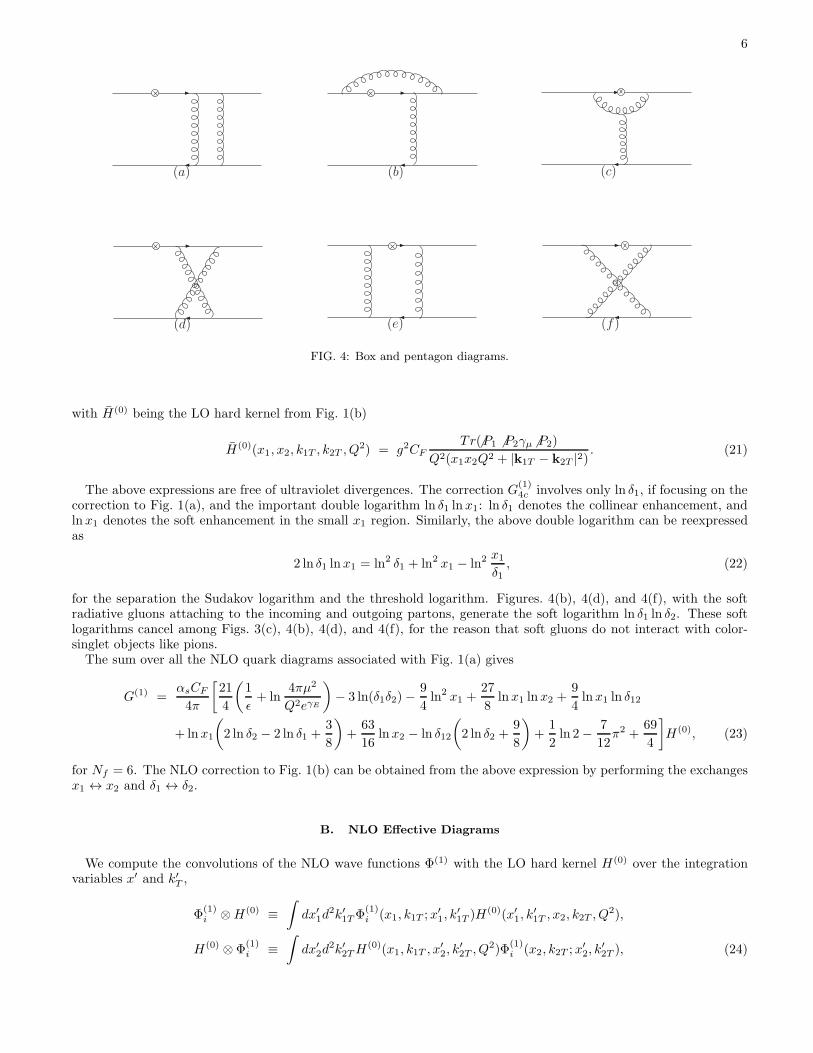
FIG. 4: Box and pentagon diagrams.

with H(0) being the LO hard kernel from Fig. 1(b)

H(0)(x1, x2, k1T , k2T , Q2) = g2CF

Tr(6 P1 6 P2γµ 6 P2)

Q2(x1x2Q2 + |k1T − k2T |2). (21)

The above expressions are free of ultraviolet divergences. The correction G(1)4c involves only ln δ1, if focusing on the

correction to Fig. 1(a), and the important double logarithm ln δ1 lnx1: ln δ1 denotes the collinear enhancement, andlnx1 denotes the soft enhancement in the small x1 region. Similarly, the above double logarithm can be reexpressedas

2 ln δ1 lnx1 = ln2 δ1 + ln2 x1 − ln2x1

δ1, (22)

for the separation the Sudakov logarithm and the threshold logarithm. Figures. 4(b), 4(d), and 4(f), with the softradiative gluons attaching to the incoming and outgoing partons, generate the soft logarithm ln δ1 ln δ2. These softlogarithms cancel among Figs. 3(c), 4(b), 4(d), and 4(f), for the reason that soft gluons do not interact with color-singlet objects like pions.The sum over all the NLO quark diagrams associated with Fig. 1(a) gives

G(1) =αsCF

4π

[

21

4

(

1

ǫ+ ln

4πµ2

Q2eγE

)

− 3 ln(δ1δ2)−9

4ln2 x1 +

27

8lnx1 lnx2 +

9

4lnx1 ln δ12

+ lnx1

(

2 ln δ2 − 2 ln δ1 +3

8

)

+63

16lnx2 − ln δ12

(

2 ln δ2 +9

8

)

+1

2ln 2− 7

12π2 +

69

4

]

H(0), (23)

for Nf = 6. The NLO correction to Fig. 1(b) can be obtained from the above expression by performing the exchangesx1 ↔ x2 and δ1 ↔ δ2.

B. NLO Effective Diagrams

We compute the convolutions of the NLO wave functions Φ(1) with the LO hard kernel H(0) over the integrationvariables x′ and k′T ,

Φ(1)i ⊗H(0) ≡

∫

dx′1d

2k′1TΦ(1)i (x1, k1T ;x

′1, k

′1T )H

(0)(x′1, k

′1T , x2, k2T , Q

2),

H(0) ⊗ Φ(1)i ≡

∫

dx′2d

2k′2TH(0)(x1, k1T , x

′2, k

′2T , Q

2)Φ(1)i (x2, k2T ;x

′2, k

′2T ), (24)

7

(g) (h)

(a)

(f)

(b) (c) (d) (e)

(i) (j)

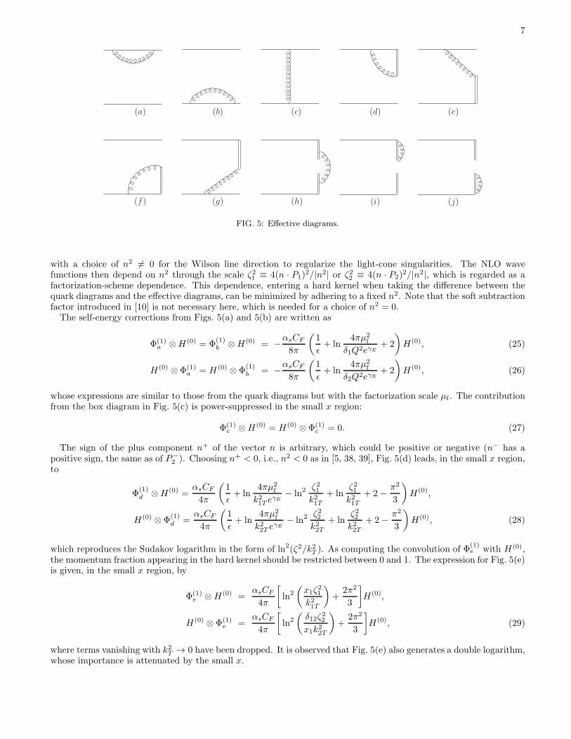
FIG. 5: Effective diagrams.

with a choice of n2 6= 0 for the Wilson line direction to regularize the light-cone singularities. The NLO wavefunctions then depend on n2 through the scale ζ21 ≡ 4(n · P1)

2/|n2| or ζ22 ≡ 4(n · P2)2/|n2|, which is regarded as a

factorization-scheme dependence. This dependence, entering a hard kernel when taking the difference between thequark diagrams and the effective diagrams, can be minimized by adhering to a fixed n2. Note that the soft subtractionfactor introduced in [10] is not necessary here, which is needed for a choice of n2 = 0.The self-energy corrections from Figs. 5(a) and 5(b) are written as

Φ(1)a ⊗H(0) = Φ

(1)b ⊗H(0) = −αsCF

8π

(

1

ǫ+ ln

4πµ2f

δ1Q2eγE

+ 2

)

H(0), (25)

H(0) ⊗ Φ(1)a = H(0) ⊗ Φ

(1)b = −αsCF

8π

(

1

ǫ+ ln

4πµ2f

δ2Q2eγE

+ 2

)

H(0), (26)

whose expressions are similar to those from the quark diagrams but with the factorization scale µf . The contributionfrom the box diagram in Fig. 5(c) is power-suppressed in the small x region:

Φ(1)c ⊗H(0) = H(0) ⊗ Φ(1)

c = 0. (27)

The sign of the plus component n+ of the vector n is arbitrary, which could be positive or negative (n− has apositive sign, the same as of P−

2 ). Choosing n+ < 0, i.e., n2 < 0 as in [5, 38, 39], Fig. 5(d) leads, in the small x region,to

Φ(1)d ⊗H(0) =

αsCF

4π

(

1

ǫ+ ln

4πµ2f

k21T eγE

− ln2ζ21k21T

+ lnζ21k21T

+ 2− π2

3

)

H(0),

H(0) ⊗ Φ(1)d =

αsCF

4π

(

1

ǫ+ ln

4πµ2f

k22T eγE

− ln2ζ22k22T

+ lnζ22k22T

+ 2− π2

3

)

H(0), (28)

which reproduces the Sudakov logarithm in the form of ln2(ζ2/k2T ). As computing the convolution of Φ(1)e with H(0),

the momentum fraction appearing in the hard kernel should be restricted between 0 and 1. The expression for Fig. 5(e)is given, in the small x region, by

Φ(1)e ⊗H(0) =

αsCF

4π

[

ln2(

x1ζ21

k21T

)

+2π2

3

]

H(0),

H(0) ⊗ Φ(1)e =

αsCF

4π

[

ln2(

δ12ζ22

x1k22T

)

+2π2

3

]

H(0), (29)

where terms vanishing with k2T → 0 have been dropped. It is observed that Fig. 5(e) also generates a double logarithm,whose importance is attenuated by the small x.

8

The result from Fig. 5(f) is similar to that from Fig. 5(d), but with the replacement of P − k by k, i.e., ζ by xζ.Keeping terms which do not vanish with k2T → 0, we have

Φ(1)f ⊗H(0) =

αsCF

4π

(

1

ǫ+ ln

4πµ2f

k21T eγE

− ln2x21ζ

21

k21T+ ln

x21ζ

21

k21T+ 2− π2

3

)

H(0),

H(0) ⊗ Φ(1)f =

αsCF

4π

(

1

ǫ+ ln

4πµ2f

k22T eγE

− ln2x22ζ

22

k22T+ ln

x22ζ

22

k22T+ 2− π2

3

)

H(0), (30)

where the double logarithm is further attenuated by x2. It should disappear, after combined with the contributionfrom Fig. 5(g), since such a double logarithm is absent in the NLO quark diagrams. The same variable transformation

relating Φ(1)f to Φ

(1)d is not applicable to Φ

(1)g , for the latter involves the nontrivial convolution with H(0). Retaining

terms which are finite as kT → 0, Fig. 5(g) leads to

Φ(1)g ⊗H(0) =

αsCF

4π

(

ln2x21ζ

21

k21T− π2

3

)

H(0),

H(0) ⊗ Φ(1)g =

αsCF

4π

(

ln2x22ζ

22

k22T− π2

3

)

H(0). (31)

It is easy to see the cancellation of the double logarithms between Eqs. (30) and (31).At last, we include the self-energy corrections to the Wilson lines, namely, Fig. 5(h-j):

Φ(1)h ⊗H(0) =

αsCF

2π

(

1

ǫ+ ln

4πµ2f

δ12Q2eγE

)

H(0),

H(0) ⊗ Φ(1)h =

αsCF

2π

(

1

ǫ+ ln

4πµ2f

δ12Q2eγE

)

H(0). (32)

Summing all the above O(αs) contributions, we obtain

Φ(1) ⊗H(0) =

h∑

i=a

Φ(1)i ⊗H(0)

=αsCF

4π

[

3

ǫ+ 3 ln

4πµ2f

ζ21eγE

+ (2 lnx1 + 3) lnζ21

δ1Q2+ 2 ln

ζ21δ12Q2

+ lnx1(lnx1 + 2) + 2− π2

3

]

H(0),

H(0) ⊗ Φ(1) =h∑

i=a

H(0) ⊗ Φ(1)i

=αsCF

4π

[

3

ǫ+ 3 ln

4πµ2f

ζ22eγE

+ (2 lnδ12x1

+ 3) lnζ22

δ2Q2+ 2 ln

ζ22δ12Q2

+ ln2δ12x1

+ 2 lnx2 + 2− π2

3

]

H(0).

(33)

The resultant anomalous dimension of the pion wave function is the same as derived in the axial gauge (for a recentreference, see [31]).

C. NLO Hard Kernel

We derive the NLO hard kernel for the pion electromagnetic form factor in the kT factorization theorem by takingthe difference between the quark and effective diagrams. Note that αs appearing in Eqs. (23) and (33) denotes thebare coupling constant, which can be rewritten as

αs = αs(µf) + δZ(µf)αs(µf), (34)

with the counterterm δZ being defined in the modified minimal subtraction scheme. We insert Eq. (34) into theexpressions of the LO and NLO quark diagrams, and of the NLO effective diagrams. The LO hard kernel H(0)

multiplied by δZ then regularizes the ultraviolet pole in Eq. (23). The ultraviolet pole in Eq. (33) is regularized bythe counterterm of the quark field and by an additive counterterm in the modified minimal subtraction scheme. For theinfrared logarithms, there exists a cancellation between the two-particle reducible quark diagrams and the two-particle

9

reducible effective diagrams. That is, G(1)2a,2b−H(0)⊗Φ

(1)a,b and G

(1)2c,2d−Φ

(1)a,b⊗H(0) are infrared finite. The self-energy

diagrams for the internal quarks and gluons are free of infrared divergences. The collinear logarithm represented by

ln δ1 (ln δ2) cancels between the two-particle irreducible diagrams and the convolution [Φ(1)d +Φ

(1)e +Φ

(1)f +Φ

(1)g ]⊗H(0)

(H(0) ⊗ [Φ(1)d +Φ

(1)e +Φ

(1)f +Φ

(1)g ]).

The infrared-finite kT -dependent NLO hard kernel for Fig. 1(a) is given by

H(1) =αs(µf)CF

4π

(

21

4ln

µ2

Q2− 6 ln

µ2f

Q2− 17

4ln2 x1 +

27

8lnx1 lnx2 − ln2 δ12 +

17

4lnx1 ln δ12

−13

8lnx1 +

31

16lnx2 +

23

8ln δ12 +

1

2ln 2 +

5π2

48+

53

4

)

H(0). (35)

We have chosen |n+| = n−, which renders ζ2 = Q2, to avoid creating an additional large logarithm like ln(ζ2/Q2).The Sudakov logarithm ln2(Q2/k2T ) in Eq. (22) has been removed by that in the effective diagrams, but the threshold

logarithms ln2 x2 remains in H(1), which can be absorbed into a jet function [37]. Because there is no end-pointsingularity in the pion form factor at twist-2, we shall not perform the factorization of this threshold logarithmhere. However, an end-point singularity does exist in the contribution from the two-parton twist-3 pion distributionamplitudes, so the factorization and the threshold resummation for the jet function needs to be performed.We have checked that Eq. (35) is gauge-invariant by repeating the NLO calculations in an arbitrary covariant gauge.

Applying the Ward identity to the gauge-dependent terms [11, 12], it is easy to show that the gauge dependence cancelsbetween the quark diagrams and the effective diagrams. The NLO hard kernel H(1) for Fig. 1(b) can be obtainedfrom Eq. (35) by exchanging x1 and x2, and by substituting H(0) in Eq. (21) for H(0). The NLO hard kernels forthe other two LO quark diagrams with the virtual photon attaching to the anti-quark line can be obtained from H(1)

and H(1) by exchanging x and 1− x.

III. NUMERICAL ANALYSIS

In this section we evaluate the NLO correction to the pion electromagnetic form factor in the kT factorization theo-rem numerically. Since the Sudakov suppression was derived in the impact parameter space, we write the factorizationformula as a convolution in the impact parameters b1 and b2 [5], conjugate to k1T and k2T , respectively. The Sudakovfactor, resulting from the summation of the double logarithm αs ln

2 kT to all orders, describes the perturbative kTdependence of a pion wave function. We shall not consider the intrinsic kT dependence of a pion wave function pro-posed in [40] here. To simplify the expression of the NLO hard kernel in the b1-b2 space, we adopt the approximationln δ12 ≈ ln(x1x2). This approximation does not modify the power-law behavior of end-point contributions from smallx, and affects numerical outcomes only slightly. We first test the following asymptotic models for the twist-2 piondistribution amplitude φA

π and the two-parton twist-3 pion distribution amplitudes φP,Tπ ,

φAπ (x) =

6fπ

2√2Nc

x(1 − x),

φPπ (x) =

fπ

2√2Nc

,

φTπ (x) =

fπ

2√2Nc

(1− 2x), (36)

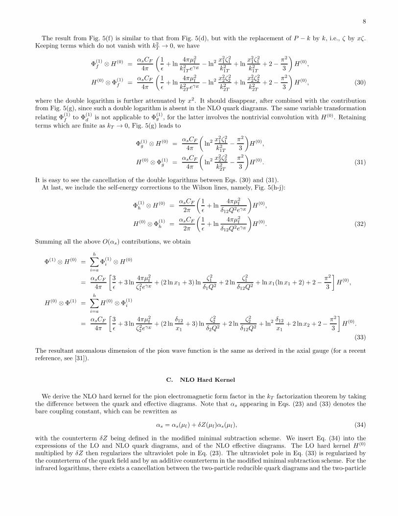
where the pion decay constant is taken as fπ = 130 MeV.The first issue concerns the choice of the renormalization scale µ and the factorization scale µf in order to minimize

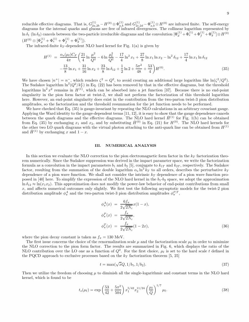
the NLO correction to the pion form factor. The results are summarized in Fig. 6, which displays the ratio of theNLO contribution over the LO one as a function of Q2. For the first choice, µf is set to the hard scale t defined inthe PQCD approach to exclusive processes based on the kT factorization theorem [5, 25]

t = max(√xQ, 1/b1, 1/b2). (37)

Then we utilize the freedom of choosing µ to diminish all the single-logarithmic and constant terms in the NLO hardkernel, which is found to be

ts(µf) = exp

(

53

42+

5π2

504

)

x5/421 x

11/242

(

µf

Q

)1/7

µf . (38)

10

0 20 40 60 80 1000.2

0.3

0.4

0.5

0.6

0.7

0.8

0.9

1.0

F NLO

tw-2(Q

2 )/ F L

O tw

-2(Q

2 )

Q2 (GeV2)

f=t, =t

s (

f)

f=Q, =t

s (

f)

=f=t

FIG. 6: Ratio of the NLO correction over the LO contribution to the pion form factor with the scale ts(µf) being defined inEq. (38).

0 1 2 3 4 5 6 7 8 9 100.0

0.1

0.2

0.3

0.4

0.5

0.6

0.7

0.8

0.9

1.0

Q2 F

(Q2 ) (

GeV

2 )

Q2 (GeV2)

LO twist-2 LO twist-2 + LO twist-3 LO twist-2 + NLO twist-2 total form factor

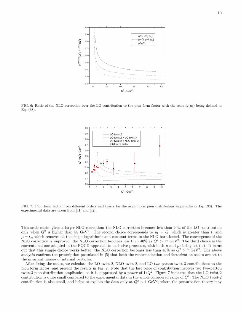
FIG. 7: Pion form factor from different orders and twists for the asymptotic pion distribution amplitudes in Eq. (36). Theexperimental data are taken from [41] and [42].

This scale choice gives a larger NLO correction: the NLO correction becomes less than 40% of the LO contributiononly when Q2 is higher than 55 GeV2. The second choice corresponds to µf = Q, which is greater than t, andµ = ts, which removes all the single-logarithmic and constant terms in the NLO hard kernel. The convergence of theNLO correction is improved: the NLO correction becomes less than 40% as Q2 > 17 GeV2. The third choice is theconventional one adopted in the PQCD approach to exclusive processes, with both µ and µf being set to t. It turnsout that this simple choice works better: the NLO correction becomes less than 40% as Q2 > 7 GeV2. The aboveanalysis confirms the prescription postulated in [5] that both the renormalization and factorization scales are set tothe invariant masses of internal particles.After fixing the scales, we calculate the LO twist-2, NLO twist-2, and LO two-parton twist-3 contributions to the

pion form factor, and present the results in Fig. 7. Note that the last piece of contribution involves two two-partontwist-3 pion distribution amplitudes, so it is suppressed by a power of 1/Q2. Figure 7 indicates that the LO twist-2contribution is quite small compared to the experimental data in the whole considered range of Q2. The NLO twist-2contribution is also small, and helps to explain the data only at Q2 ∼ 1 GeV2, where the perturbation theory may

11

0 1 2 3 4 5 6 7 8 9 100.0

0.2

0.4

0.6

0.8

1.0

1.2

1.4

Q2 F

(Q2 ) (

GeV

2 )

Q2 (GeV2)

LO twist-2 LO twist-2 + LO twist-3 LO twist-2 + NLO twist-2 total form factor

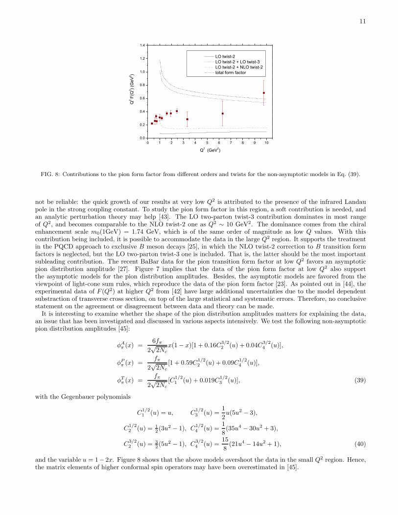
FIG. 8: Contributions to the pion form factor from different orders and twists for the non-asymptotic models in Eq. (39).

not be reliable: the quick growth of our results at very low Q2 is attributed to the presence of the infrared Landaupole in the strong coupling constant. To study the pion form factor in this region, a soft contribution is needed, andan analytic perturbation theory may help [43]. The LO two-parton twist-3 contribution dominates in most rangeof Q2, and becomes comparable to the NLO twist-2 one as Q2 ∼ 10 GeV2. The dominance comes from the chiralenhancement scale m0(1GeV) = 1.74 GeV, which is of the same order of magnitude as low Q values. With thiscontribution being included, it is possible to accommodate the data in the large Q2 region. It supports the treatmentin the PQCD approach to exclusive B meson decays [25], in which the NLO twist-2 correction to B transition formfactors is neglected, but the LO two-parton twist-3 one is included. That is, the latter should be the most importantsubleading contribution. The recent BaBar data for the pion transition form factor at low Q2 favors an asymptoticpion distribution amplitude [27]. Figure 7 implies that the data of the pion form factor at low Q2 also supportthe asymptotic models for the pion distribution amplitudes. Besides, the asymptotic models are favored from theviewpoint of light-cone sum rules, which reproduce the data of the pion form factor [23]. As pointed out in [44], theexperimental data of F (Q2) at higher Q2 from [42] have large additional uncertainties due to the model dependentsubstraction of transverse cross section, on top of the large statistical and systematic errors. Therefore, no conclusivestatement on the agreement or disagreement between data and theory can be made.It is interesting to examine whether the shape of the pion distribution amplitudes matters for explaining the data,

an issue that has been investigated and discussed in various aspects intensively. We test the following non-asymptoticpion distribution amplitudes [45]:

φAπ (x) =

6fπ

2√2Nc

x(1− x)[1 + 0.16C3/22 (u) + 0.04C

3/24 (u)],

φPπ (x) =

fπ

2√2Nc

[1 + 0.59C1/22 (u) + 0.09C

1/24 (u)],

φTπ (x) =

fπ

2√2Nc

[C1/21 (u) + 0.019C

1/23 (u)], (39)

with the Gegenbauer polynomials

C1/21 (u) = u, C

1/23 (u) =

1

2u(5u2 − 3),

C1/22 (u) = 1

2 (3u2 − 1), C

1/24 (u) =

1

8(35u4 − 30u2 + 3),

C3/22 (u) = 3

2 (5u2 − 1), C

3/24 (u) =

15

8(21u4 − 14u2 + 1), (40)

and the variable u = 1− 2x. Figure 8 shows that the above models overshoot the data in the small Q2 region. Hence,the matrix elements of higher conformal spin operators may have been overestimated in [45].

12

0 10 20 30 40 50 60 70 80 90 1000.1

0.2

0.3

0.4

0.5

Q2 F

(Q2 )

(GeV

2 )

Q2 (GeV2)

f=t, =t

s (

f)

f=Q, =t

s (

f)

=f=t

FIG. 9: Scale dependence of the pion form factor with ts(µf) being defined in Eq. (38).

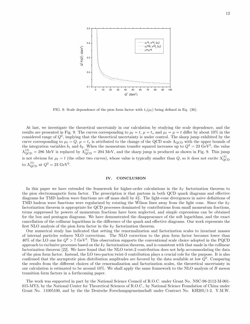
At last, we investigate the theoretical uncertainly in our calculation by studying the scale dependence, and theresults are presented in Fig. 9. The curves corresponding to µf = t, µ = ts and µf = µ = t differ by about 10% in theconsidered range of Q2, implying that the theoretical uncertainty is under control. The sharp jump exhibited by thecurve corresponding to µf = Q, µ = ts is attributed to the change of the QCD scale ΛQCD with the upper bounds ofthe integration variables b1 and b2. When the momentum transfer squared increases up to Q2 = 23 GeV2, the value

Λ(4)QCD = 286 MeV is replaced by Λ

(5)QCD = 204 MeV, and the sharp jump is produced as shown in Fig. 9. This jump

is not obvious for µf = t (the other two curves), whose value is typically smaller than Q, so it does not excite Λ(4)QCD

to Λ(5)QCD at Q2 = 23 GeV2.

IV. CONCLUSION

In this paper we have extended the framework for higher-order calculations in the kT factorization theorem tothe pion electromagnetic form factor. The prescription is that partons in both QCD quark diagrams and effectivediagrams for TMD hadron wave functions are off mass shell by k2T . The light-cone divergences in naive definitions ofTMD hadron wave functions were regularized by rotating the Wilson lines away from the light cone. Since the kTfactorization theorem is appropriate for QCD processes dominated by contributions from small momentum fractions,terms suppressed by powers of momentum fractions have been neglected, and simple expressions can be obtainedfor the box and pentagon diagrams. We have demonstrated the disappearance of the soft logarithms, and the exactcancellation of the collinear logarithms in the difference of the quark and effective diagrams. Our work represents thefirst NLO analysis of the pion form factor in the kT factorization theorem.Our numerical study has indicated that setting the renormalization and factorization scales to invariant masses

of internal particles reduces NLO corrections. The NLO correction to the pion form factor becomes lower than40% of the LO one for Q2 > 7 GeV2. This observation supports the conventional scale choice adopted in the PQCDapproach to exclusive processes based on the kT factorization theorem, and is consistent with that made in the collinearfactorization theorem [22]. We have found that the NLO twist-2 contribution does not help accommodating the dataof the pion form factor. Instead, the LO two-parton twist-3 contribution plays a crucial role for the purpose. It is alsoconfirmed that the asymptotic pion distribution amplitudes are favored by the data available at low Q2. Comparingthe results from the different choices of the renormalization and factorization scales, the theoretical uncertainty inour calculation is estimated to be around 10%. We shall apply the same framework to the NLO analysis of B mesontransition form factors in a forthcoming paper.

The work was supported in part by the National Science Council of R.O.C. under Grant No. NSC-98-2112-M-001-015-MY3, by the National Center for Theoretical Sciences of R.O.C., by National Science Foundation of China underGrant No. 11005100, and by the the Deutsche Forschungsgemeinschaft under Contract No. KH205/1-2. Y.M.W.

13

would like to acknowledge Prof. Cai-Dian Lu for warm hospitality during his visit at IHEP, Beijing, and Prof.Xue-Qian Li for inviting him to give a talk at Nankai University.

[1] S. Catani, M. Ciafaloni and F. Hautmann, Phys. Lett. B 242, 97 (1990); Nucl. Phys. B 366, 135 (1991).[2] J.C. Collins and R.K. Ellis, Nucl. Phys. B 360, 3 (1991).[3] E.M. Levin, M.G. Ryskin, Yu.M. Shabelskii, and A.G. Shuvaev, Sov. J. Nucl. Phys. 53, 657 (1991).[4] J. Botts and G. Sterman, Nucl. Phys. B 225, 62 (1989).[5] H-n. Li and G. Sterman, Nucl. Phys. B 381, 129 (1992).[6] T. Huang and Q.X. Shen, Z. Phys. C 50, 139 (1991); J.P. Ralston and B. Pire, Phys. Rev. Lett. 65, 2343 (1990).[7] F. Dominguez, B.W. Xiao, and F. Yuan, Phys. Rev. Lett. 106, 022301 (2011).[8] S.P. Baranov, A.V. Lipatov, and N.P. Zotov, arXiv:1012.3022 [hep-ph]; A.V. Lipatov, M.A. Malyshev, and N.P. Zotov,

arXiv:1102.1134 [hep-ph].[9] M. Nagashima and H-n. Li, Phys. Rev. D 67, 034001 (2003).

[10] F. Feng, J. P. Ma and Q. Wang, Phys. Lett. B 674, 176 (2009).[11] S. Nandi and H-n. Li, Phys. Rev. D 76, 034008 (2007).[12] H-n. Li and S. Mishima, Phys. Lett. B 674, 182 (2009).[13] J.C. Collins, Acta. Phys. Polon. B 34, 3103 (2003).[14] J.P. Ma and Q. Wang, JHEP 0601, 067 (2006); Phys. Lett. B 642, 232 (2006).[15] H-n. Li and H.S. Liao, Phys. Rev. D 70, 074030 (2004).[16] R.D. Field, R. Gupta, S. Otto, and L. Chang, Nucl. Phys. B 186, 429 (1981).[17] F.M. Dittes and A.V. Radyushkin, Yad. Fiz. 34, 529 (1981) [Sov. J. Nucl. Phys. 34, 293 (1981)].[18] M.H. Sarmadi, Ph.D. thesis, University of Pittsburgh, 1982.[19] R.S. Khalmuradov and A.V. Radyushkin, Yad. Fiz. 42, 458 (1985), [Sov. J. Nucl. Phys. 42, 289 (1985)].[20] E. Braaten and S.M. Tse, Phys. Rev. D 35, 2255 (1987).[21] E.P. Kadantseva, S.V. Mikhailov, and A.V. Radyushkin, Yad. Fiz. 44, 507 (1986) [Sov. J. Nucl. Phys. 44, 326 (1986)].[22] B. Melic, B. Nizic, and K. Passek, Phys. Rev. D 60, 074004 (1999).[23] V. M. Braun, A. Khodjamirian and M. Maul, Phys. Rev. D 61, 073004 (2000).[24] J. Bijnens and A. Khodjamirian, Eur. Phys. J. C 26, 67 (2002).[25] Y.Y. Keum, H-n. Li, and A.I. Sanda, Phys. Lett. B 504, 6 (2001); Phys. Rev. D 63, 054008 (2001); Y.Y. Keum and H-n.

Li, Phys. Rev. D 63, 074006 (2001); C. D. Lu, K. Ukai and M. Z. Yang, Phys. Rev. D 63, 074009 (2001).[26] H-n. Li and S. Mishima, Phys. Rev. D 80, 074024 (2009).[27] B. Aubert et al. [The BABAR Collaboration], Phys. Rev. D 80, 052002 (2009).[28] Z.T. Wei and M.Z. Yang, Phys. Rev. D 67, 094013 (2003); J.W. Chen, H. Kohyama, K. Ohnishi, U. Raha, and Y.L. Shen,

Phys. Lett. B 693, 102 (2010).[29] H-n. Li, Phys. Rev. D 64, 014019 (2001); M. Nagashima and H-n. Li, Eur. Phys. J. C 40, 395 (2005).[30] X. Ji, and F. Yuan, Phys. Lett. B 543, 66 (2002); A.V. Belitsky, X. Ji, and F. Yuan, Nucl. Phys. B 656, 165 (2003).[31] I. O. Cherednikov and N. G. Stefanis, Nucl. Phys. B 802, 146 (2008).[32] W. Siegel, Phys. Lett. B 84, 193 (1979).[33] J.C. Collins and D.E. Soper, Nucl. Phys. B 193, 381 (1981).[34] G.P. Korchemsky, D. Pirjol, and T.M. Yan, Phys. Rev. D 61, 114510 (2000) and references therein.[35] J.P. Ma and Q. Wang, Phys. Rev. D 75, 014014 (2007) and references therein.[36] R. Akhoury, G. F. Sterman and Y. P. Yao, Phys. Rev. D 50, 358 (1994).[37] H-n. Li, Phys. Rev. D 66, 094010 (2002); K. Ukai and H-n. Li, Phys. Lett. B 555, 197 (2003).[38] H-n. Li and H.L. Yu, Phys. Rev. Lett. 74, 4388 (1995); Phys. Lett. B 353, 301 (1995); Phys. Rev. D 53, 2480 (1996).[39] H-n. Li, Phys. Rev. D 55, 105 (1997).[40] R. Jakob and P. Kroll, Phys. Lett. B 315, 463 (1993); B 319, 545 (1993)(E).[41] G. M. Huber et al. [Jefferson Lab Collaboration], Phys. Rev. C 78, 045203 (2008).[42] C. J. Bebek et al., Phys. Rev. D 17, 1693 (1978).[43] A. P. Bakulev, K. Passek-Kumericki, W. Schroers and N. G. Stefanis, Phys. Rev. D 70, 033014 (2004) [Erratum-ibid. D

70, 079906 (2004)].[44] H. P. Blok, G. M. Huber and D. J. Mack, arXiv:nucl-ex/0208011.[45] G. Duplancic, A. Khodjamirian, T. Mannel, B. Melic, and N. Offen, JHEP 0804, 014 (2008).