Citation: Yang, J.; Li, X.; Luo, L.;

Zhao, L.; Wei, J.; Ma, T. New

Supplementary Photography

Methods after the Anomalous of

Ground Control Points in UAV

Structure-from-Motion

Photogrammetry. Drones 2022, 6, 105.

https://doi.org/10.3390/

drones6050105

Academic Editors: Efstratios

Stylianidis and Luis Javier

Sánchez-Aparicio

Received: 20 March 2022

Accepted: 21 April 2022

Published: 24 April 2022

Publisher’s Note: MDPI stays neutral

with regard to jurisdictional claims in

published maps and institutional affil-

iations.

Copyright: © 2022 by the authors.

Licensee MDPI, Basel, Switzerland.

This article is an open access article

distributed under the terms and

conditions of the Creative Commons

Attribution (CC BY) license (https://

creativecommons.org/licenses/by/

4.0/).

drones

Article

New Supplementary Photography Methods after theAnomalous of Ground Control Points in UAVStructure-from-Motion PhotogrammetryJia Yang 1,*,†, Xiaopeng Li 1,2,†, Lei Luo 3 , Lewen Zhao 1, Juan Wei 1 and Teng Ma 1

1 School of Surveying and Urban Spatial Information, Henan University of Urban Construction,Pingdingshan 467036, China; lixp@gs.zzu.edu.cn (X.L.); 202012263@hncj.edu.cn (L.Z.);065418122@hncj.edu.cn (J.W.); 202012140@hncj.edu.cn (T.M.)

2 School of Geoscience and Technology, Zhengzhou University, Zhengzhou 450001, China3 Aerospace Information Research Institute, Chinese Academy of Sciences, Beijing 100094, China;

luolei@aircas.ac.cn* Correspondence: yangjia@hncj.edu.cn† These authors contributed equally to this work.

Abstract: Recently, multirotor UAVs have been widely used in high-precision terrain mapping,cadastral surveys and other fields due to their low cost, flexibility, and high efficiency. Indirectgeoreferencing of ground control points (GCPs) is often required to obtain highly accurate topographicproducts such as orthoimages and digital surface models. However, in practical projects, GCPs aresusceptible to anomalies caused by external factors (GCPs covered by foreign objects such as crops andcars, vandalism, etc.), resulting in a reduced availability of UAV images. The errors associated with theloss of GCPs are apparent. The widely used solution of using natural feature points as ground controlpoints often fails to meet the high accuracy requirements. For the problem of control point anomalies,this paper innovatively presents two new methods of completing data fusion by supplementingphotos via UAV at a later stage. In this study, 72 sets of experiments were set up, including threecontrol experiments for analysis. Two parameters were used for accuracy assessment: Root MeanSquare Error (RMSE) and Multiscale Model to Model Cloud Comparison (M3C2). The study showsthat the two new methods can meet the reference accuracy requirements in horizontal directionand elevation direction (RMSEX = 70.40 mm, RMSEY = 53.90 mm, RMSEZ = 87.70 mm). In contrast,the natural feature points as ground control points showed poor accuracy, with RMSEX = 94.80 mm,RMSEY = 68.80 mm, and RMSEZ = 104.40 mm for the checkpoints. This research considers andsolves the problems of anomalous GCPs in the photogrammetry project from a unique perspectiveof supplementary photography, and proposes two new methods that greatly expand the meansof solving the problem. In UAV high-precision projects, they can be used as an effective meansto ensure accuracy when the GCP is anomalous, which has significant potential for applicationpromotion. Compared with previous methods, they can be applied in more scenarios and havehigher compatibility and operability. These two methods can be widely applied in cadastral surveys,geomorphological surveys, heritage conservation, and other fields.

Keywords: unmanned aerial vehicle (UAV); structure-from-motion (SFM); accuracy assessment;ground control points (GCP)

1. Introduction

With the rapid development of UAV hardware and ground-station software tech-nology, UAVs have become smarter and have an increasingly wide range of applications.Using UAV to acquire earth observation data combined with a structure-from-motion (SFM)algorithm can generate high-precision orthoimages and digital surface models (DSM). Thepoints on the house wall, building corners [1], or farmland [2] on the orthoimages can be

Drones 2022, 6, 105. https://doi.org/10.3390/drones6050105 https://www.mdpi.com/journal/drones

Drones 2022, 6, 105 2 of 22

collected to obtain ownership information. Based on ensuring satisfactory accuracy, theefficiency of cadastral survey work in cities [3] and rural areas is greatly improved. Ingeomorphology [4–6], multiphase photogrammetric point cloud data is generated. Thechanges are monitored and analyzed by obtaining aerial photos of different phases of land-forms such as river channel morphology, glaciers, and landslides. Digital reconstruction ofhistorical buildings is carried out by combining the photo datasets collected by UAVs andthe hand-held camera [7–9]. Accurate building size and texture information are obtainedto facilitate the protection and maintenance of historic buildings. At the same time, it canalso combine virtual reality (VR) and augmented reality (AR) technology to popularizeancient buildings.

In the field of precision agriculture [10–13], the use of UAV photogrammetry allowsfor the generation of crop height models (CHMs), which are one of the most importantparameters for assessing crop characteristics such as biomass, leaf area index (LAI), andyield. In hilly and mountainous areas, drones can also obtain high-level terrain detail toprovide more accurate basic geographic data for mechanized agriculture. In the field oflarge-scale infrastructure construction [14–18], UAVs play an increasingly important role.They can complete a mine topographic survey and a fill-and-excavation volume monitoringand evaluation and perform change monitoring, progress monitoring, and site-planning onconstruction sites such as roads, bridges, and buildings, thus saving corresponding laborand time costs and improving production efficiency.

The UAV Post-Processed Kinematic (PPK) and Real-Time Kinematic (RTK) technolo-gies are gradually maturing, and the research related to them is also increasing. Manystudies [19–23] have shown that using UAVs equipped with GNSS RTK can effectivelyimprove the planimetric accuracy. The accuracy is very close to that of the project using areasonable GCPs distribution. However, the elevation error varies significantly dependingon the experimental equipment and studied surface morphology, showing the phenomenonof unstable elevation accuracy. To improve the elevation accuracy of direct georeferencing,a dual-grid oblique flight in differential mode can achieve the approximate planimetricand vertical accuracy of the deployment GCP scheme. While in RTK compared to PPK,the accuracy is higher in the single-grid nadiral flight model, where both planimetric andelevation differences are poor. The addition of partial oblique data improves the elevationaccuracy significantly, with significant errors in the N direction [24]. In contrast, whenusing RTK-UAV direct georeferencing, the combination scheme between orthoimages withdifferent aerial heights and the combination scheme between different oblique images inthe urban surface study area can be evaluated with higher accuracy. However, it showsdifferent trends in the countryside, with better accuracy performance only when combiningnadiral images with oblique images [25]. However, there are some limitations to this tech-nology. RTK real-time differential correction is available in two ways, local main RTK orcontinuously operating reference station (CORS) network transmission (NRTK). The NRTK,however, is affected by the strength of the network signal, and observations may be unfixed,resulting in errors. With the PPK method, there is no risk of data accuracy degradation dueto interruptions in network transmission. Still, the accuracy of the PPK method may beadversely affected by the long reference distance if the UAV´s flight path has a long path(>30 km) [26]. In practice, most of the sensors carried by UAVs are non-professional mea-surement cameras. In some areas where the surface is relatively flat, direct georeferencingcan easily lead to the dome effect, which is caused by anomalies in the internal orientationelements of the camera calibration [27]. In summary, the involvement of ground controlpoints is still required for geomorphological surveys to meet high accuracy requirements.

The existing photogrammetric GCP studies have mainly focused on the influence ofthe distribution and number of GCPs on the measurement accuracy. Most researchersassume that the higher the number of control points used, the better the overall accuracy.Oniga et al. [28] considered it necessary to have GCPs not far from the corners of the studyarea. When the number of GCPs was increased from 8 to 20, the accuracy greatly improvedbut continued to increase the number of GCPs—the trend of accuracy improvement slowed

Drones 2022, 6, 105 3 of 22

down. Eventually, the planimetric accuracy of the RMSE gradually approached two timesthe GSD, and the elevation accuracy of the RMSE approached three times the GSD. Sanz-Ablanedo et al. [29] deployed 102 GCPs in a 1225 ha coal-mine area, and when 10–20 GCPswere used, the RMSE of the checkpoints was approximately five times the project averageGSD. By adding more GCPs to reach more than two GCPs per 100 photos, the RMSE slowlyconverges to a value approximately twice the average GSD.

At the same time, the GCPs should be uniformly distributed throughout the studyarea, preferably in a triangular grid structure. This configuration minimizes the maximumdistance of any GCPs in the area. Ferrer-González et al. [30] proposed that both horizontaland vertical accuracy in the case of a corridor´s survey area increases with the number ofGCPs used in bundle adjustment, and that planar accuracy is always better than verticalaccuracy. Placing GCPs on the edge of the corridor alternately and placing two GCPs ateach end of the study area produced the most accurate results. Liu et al. [31] also concludedthat GCPs should be evenly distributed over the study area, with at least one GCP near thecenter of the area. The local accuracy of DSM decreased significantly when the distancebetween the adjacent GCPs increased. Ulvi [32] proposed that if the GCPs are concentratedin the center, the planimetric and elevation accuracy of all inspection points in the surveyarea is the worst, and the GCPs placed at the edge of the study area can obtain the bestplanimetric accuracy but cannot obtain the best elevation accuracy. When the number ofGCPs is increased in the center of the study area, the overall error can be minimized andthe best elevation accuracy can be obtained.

There has been a significant number of studies on GCPs; both manually placed GCPsand natural feature points are subject to anomalies due to natural and human factors.However, there is a lack of systematic research on GCP anomalies during UAV collectiondata. Common GCP anomalies often occur when covered by foreign objects such asvehicles, crops, and vandalism (Figure 1). In UAV aerial photogrammetry, GCPs areoften placed first. Then, the route task is carried out to collect aerial photographs, so thesequence of operations will bring the possibility of GCPs anomalies. Anomalies in theGCPs often cause irreversible damage to the operation in that the GCPs cannot be found inthe completed aerials.

Drones 2022, 6, x FOR PEER REVIEW 4 of 24

(a) (b) (c)

Figure 1. Illustration of anomalous ground control points: (a) car gland; (b) crop gland; (c) vandal-ism (being cleaned).

This paper proposes two solutions in UAV photogrammetry for this anomalous GCP to solve these problems. The surface information of the processed anomalous GCP is com-plemented by our method and then fused into the nadiral images to achieve the purpose of indirect georeferencing of this GCP, which ensures the accuracy and quality of the data. An innovative way of thinking about problems and solving them from a new perspective is the use of a supplementary photograph. Compared with the previous solutions, the proposed methods can actively perform post-secondary work supplementary photog-raphy for anomalous GCPs, which is more controllable and can be applied to more envi-ronmental scenarios. At the same time, in the practical operation of the methods, it is more fault-tolerant and operative and can efficiently complete the supplementary photography of the anomalous GCPs. New ideas and methods are provided for solving GCPs anoma-lies in practical UAV photogrammetry projects. The new methods can be widely used in cadastral surveying, high-precision topographic mapping, and other fields.

2. Materials and Methods 2.1. Study Area

The study area is located in Yanglingzhuang Village, Yexian County, Pingdingshan City, Henan Province, China (Figure 2). The east–west length is about 880 m, the north–south length is about 870 m, and the elevation range is from 154 to 185 m. The longitude range of the study area is 113°13′27″ E~113°14′02″ E, and the latitude range is 33°25′47″ N~33°26′13″ N, with an area of 0.67 km². The study area contains various feature elements, such as arable land, rivers, artificial structures, scrubland, and groves, which are more representative. The wide field of view of the flight and the uninterrupted satellite signal are conducive to collecting images by the UAV.

Figure 1. Illustration of anomalous ground control points: (a) car gland; (b) crop gland; (c) vandalism(being cleaned).

A widely used method is to find a natural feature around an anomalous GCP toreplace that anomaly and achieve indirect georeferencing of the GCPs by reacquiringthe geographic coordinates of that natural feature and transcribing them to the initialphotograph. However, this method is more dependent on the quality of the natural featurepoints and the subjective judgement of the data processor. However, it is impossible to findnatural feature points that meet the standards in many places. Boon et al. [33] suggestedusing artificially marked GCPs and Checkpoints (CPs) instead of natural feature points.Forlani et al. [22] proposed that artificially marked GCPs are necessary because it is difficultto find natural feature points of the required quality in areas outside of cities. Therefore,in applications such as high-precision topographic mapping, artificially marked groundcontrol points should be used as much as possible. Natural feature points on the groundoften have many uncontrollable factors and drawbacks.

Drones 2022, 6, 105 4 of 22

This paper proposes two solutions in UAV photogrammetry for this anomalous GCPto solve these problems. The surface information of the processed anomalous GCP iscomplemented by our method and then fused into the nadiral images to achieve thepurpose of indirect georeferencing of this GCP, which ensures the accuracy and qualityof the data. An innovative way of thinking about problems and solving them from anew perspective is the use of a supplementary photograph. Compared with the previoussolutions, the proposed methods can actively perform post-secondary work supplementaryphotography for anomalous GCPs, which is more controllable and can be applied to moreenvironmental scenarios. At the same time, in the practical operation of the methods,it is more fault-tolerant and operative and can efficiently complete the supplementaryphotography of the anomalous GCPs. New ideas and methods are provided for solvingGCPs anomalies in practical UAV photogrammetry projects. The new methods can bewidely used in cadastral surveying, high-precision topographic mapping, and other fields.

2. Materials and Methods2.1. Study Area

The study area is located in Yanglingzhuang Village, Yexian County, PingdingshanCity, Henan Province, China (Figure 2). The east–west length is about 880 m, the north–south length is about 870 m, and the elevation range is from 154 to 185 m. The longituderange of the study area is 113◦13′27′′ E~113◦14′02′′ E, and the latitude range is 33◦25′47′′

N~33◦26′13′′ N, with an area of 0.67 km2. The study area contains various feature elements,such as arable land, rivers, artificial structures, scrubland, and groves, which are morerepresentative. The wide field of view of the flight and the uninterrupted satellite signalare conducive to collecting images by the UAV.

Drones 2022, 6, x FOR PEER REVIEW 5 of 24

Figure 2. Location of the study area. The orthophoto illustrates the study area surrounded by a red polyline.

2.2. Overall Workflow The process of this research (Figure 3) can be divided into three parts, including data

acquisition, data processing, and accuracy evaluation. Our proposed solution and the com-parison scheme are processed separately by structure from motion (SFM) and multiview stereopsis (MVS), and the results of the different schemes are evaluated for accuracy after the point clouds are generated. The main evaluation metrics include RMSE and M3C2 dis-tance.

Figure 3. Overall experimental workflow. Group I used the “STNG” method, and Group II used the “Oblique and Circle” method.

Figure 2. Location of the study area. The orthophoto illustrates the study area surrounded by ared polyline.

2.2. Overall Workflow

The process of this research (Figure 3) can be divided into three parts, includingdata acquisition, data processing, and accuracy evaluation. Our proposed solution andthe comparison scheme are processed separately by structure from motion (SFM) andmultiview stereopsis (MVS), and the results of the different schemes are evaluated for

Drones 2022, 6, 105 5 of 22

accuracy after the point clouds are generated. The main evaluation metrics include RMSEand M3C2 distance.

Drones 2022, 6, x FOR PEER REVIEW 5 of 24

Figure 2. Location of the study area. The orthophoto illustrates the study area surrounded by a red polyline.

2.2. Overall Workflow The process of this research (Figure 3) can be divided into three parts, including data

acquisition, data processing, and accuracy evaluation. Our proposed solution and the com-parison scheme are processed separately by structure from motion (SFM) and multiview stereopsis (MVS), and the results of the different schemes are evaluated for accuracy after the point clouds are generated. The main evaluation metrics include RMSE and M3C2 dis-tance.

Figure 3. Overall experimental workflow. Group I used the “STNG” method, and Group II used the “Oblique and Circle” method.

Figure 3. Overall experimental workflow. Group I used the “STNG” method, and Group II used the“Oblique and Circle” method.

There is often a time lag between the placing of GCPs and UAV operations in UAVphotogrammetry. During this time gap, GCPs are prone to be vandalised or covered byforeign objects. These problems are not easily detected during the flight of the UAV route,resulting in a reduced availability of the images due to that anomalous GCPs. In order tosolve the problem of anomalous GCPs, we proposed two methods called the “STNG” andthe “Oblique and Circle”.

“STNG” is a method of taking photographs by descending equidistantly and verticallyfrom sky to near-ground (Figure 4). We defined a specific altitude, H1, directly abovethe restored GCP as the starting point (H1 = H + ∆h, where H is the orthometric altitudeand ∆h is the difference between the altitude of the orthometric take-off point and thealtitude of the anomalous control point). We then hovered at certain intervals D to takepictures during the vertical downward movement of the UAV until it reached the surfaceto complete the operation.

“Oblique and Circle” is a method of surround photography that maintains the obliqueangle of the camera for anomalous GCP (Figure 5). We defined that the position of H2(same as H1) directly above the repaired GCP was the centre O, a certain distance R wasthe radius to make a circular motion, and the camera was inclined at a certain angle β. Theheading angle α was a fixed interval to take images. The main optical axis of the camerawas required to align with the GCP.

Drones 2022, 6, 105 6 of 22

Drones 2022, 6, x FOR PEER REVIEW 6 of 24

There is often a time lag between the placing of GCPs and UAV operations in UAV photogrammetry. During this time gap, GCPs are prone to be vandalised or covered by foreign objects. These problems are not easily detected during the flight of the UAV route, resulting in a reduced availability of the images due to that anomalous GCPs. In order to solve the problem of anomalous GCPs, we proposed two methods called the “STNG” and the “Oblique and Circle”.

“STNG” is a method of taking photographs by descending equidistantly and verti-cally from sky to near-ground (Figure 4). We defined a specific altitude, H1, directly above the restored GCP as the starting point (H1 = H + Δh, where H is the orthometric altitude and Δh is the difference between the altitude of the orthometric take-off point and the altitude of the anomalous control point). We then hovered at certain intervals D to take pictures during the vertical downward movement of the UAV until it reached the surface to complete the operation.

Figure 4. Demonstration of the principle of the “STNG” method.

“Oblique and Circle” is a method of surround photography that maintains the oblique angle of the camera for anomalous GCP (Figure 5). We defined that the position of H2 (same as H1) directly above the repaired GCP was the centre O, a certain distance R was the radius to make a circular motion, and the camera was inclined at a certain angle β. The heading angle α was a fixed interval to take images. The main optical axis of the camera was required to align with the GCP.

Figure 4. Demonstration of the principle of the “STNG” method.

Drones 2022, 6, x FOR PEER REVIEW 7 of 24

Figure 5. Demonstration of the principle of the “Oblique and Circle” method.

2.3. Data Collection 2.3.1. GNSS Survey

According to the characteristics of the field to be studied, we used four corner points combined with a central point to place a total of five GCPs [34]. In order to assess the accuracy, the checkpoints were placed evenly over the study area with a total of 19 CPs (Figure 6). In addition, we searched for the ground natural feature point (the corner point of the bridge named TZ2) near point K2 as a GCP instead of point K2. As the study area is located in the countryside, with more cultivated land and abundant natural landforms, we compared several locations. Finally, we chose the bridge corner point with a high level and more flat terrain as the natural feature point. Two materials were used to place the GCPs and CPs, i.e., pulverized lime for the dirt roads and red paint for the concrete roads.

Figure 5. Demonstration of the principle of the “Oblique and Circle” method.

2.3. Data Collection2.3.1. GNSS Survey

According to the characteristics of the field to be studied, we used four corner pointscombined with a central point to place a total of five GCPs [34]. In order to assess theaccuracy, the checkpoints were placed evenly over the study area with a total of 19 CPs(Figure 6). In addition, we searched for the ground natural feature point (the corner pointof the bridge named TZ2) near point K2 as a GCP instead of point K2. As the study area islocated in the countryside, with more cultivated land and abundant natural landforms, wecompared several locations. Finally, we chose the bridge corner point with a high level and

Drones 2022, 6, 105 7 of 22

more flat terrain as the natural feature point. Two materials were used to place the GCPsand CPs, i.e., pulverized lime for the dirt roads and red paint for the concrete roads.

Drones 2022, 6, x FOR PEER REVIEW 8 of 24

Figure 6. Shows the route and take-off point of the UAV; the map also shows the distribution of ground control points, checkpoints, and natural feature points.

Three measurements of 24 artificial GCPs and one natural feature point were made in CORS mode using a Huace i80 GNSS receiver. The spatial reference was the CGCS 2000 ellipsoid, the projection was the Gauss–Kruger projection, and the elevation datum was “National Vertical Datum 1985”—all in metres (m). Each positioning was verified to be above 12 satellites, with 10 ephemerides collected each time. The device achieved a hori-zontal accuracy of ± (8 + 0.5 × 10−6 × D) mm and a vertical accuracy of ± (15 + 0.5 × 10−6 × D) mm in CORS mode.

2.3.2. UAV Image Acquisition The photographs for this experiment were collected using a DJI Phantom 4 Pro drone

manufactured by DJI. It is a consumer-grade UAV that is portable, flexible, small in weight and low in cost. It carries a DJI FC6310 camera with a field of view (FOV) of 84° and an image size of 5472 × 3648 pixels. The route planning software used for the experiment was DJI Pilot and DJI GO4. The study area boundary was converted to KML format and im-ported into DJI Pilot software, the flight altitude (H) above the ground was set to 160 m, the forward overlap was 80%, the side overlap was 80%, the Mapping Mode was set, and the take-off point was selected as point K5 (the altitude of this point is 159.8 m). The cam-era parameter settings (ISO and exposure values, etc.) are automatically adjusted accord-ing to the actual brightness of the scene at the time of flight. The experiment was com-pleted on 4 July 2021 with a light breeze and good light at the site. We collected a total of 562 nadiral images with an average ground resolution of 4.32 cm/pixel. The route and images are shown in Figure 6.

After the nadiral images were acquired, the anomalous GCP was photographed us-ing the method proposed in this paper. As the anomaly GCP (K2) was at the same altitude as the ortho take-off point (K5), the starting flight altitude above the ground for data col-lection was 160 m (nadiral flight altitude), and then hovered every 5 m down to take one photo for a total of 32 images. The DJI GO4 software was used to complete the data acqui-sition and determine the height of descent based on the value shown on the display.

Figure 6. Shows the route and take-off point of the UAV; the map also shows the distribution ofground control points, checkpoints, and natural feature points.

Three measurements of 24 artificial GCPs and one natural feature point were made inCORS mode using a Huace i80 GNSS receiver. The spatial reference was the CGCS 2000 el-lipsoid, the projection was the Gauss—Kruger projection, and the elevation datum was “Na-tional Vertical Datum 1985”—all in metres (m). Each positioning was verified to be above12 satellites, with 10 ephemerides collected each time. The device achieved a horizontal ac-curacy of±(8 + 0.5× 10−6 × D) mm and a vertical accuracy of±(15 + 0.5 × 10−6 × D) mmin CORS mode.

2.3.2. UAV Image Acquisition

The photographs for this experiment were collected using a DJI Phantom 4 Pro dronemanufactured by DJI. It is a consumer-grade UAV that is portable, flexible, small in weightand low in cost. It carries a DJI FC6310 camera with a field of view (FOV) of 84◦ and animage size of 5472 × 3648 pixels. The route planning software used for the experimentwas DJI Pilot and DJI GO4. The study area boundary was converted to KML format andimported into DJI Pilot software, the flight altitude (H) above the ground was set to 160 m,the forward overlap was 80%, the side overlap was 80%, the Mapping Mode was set, andthe take-off point was selected as point K5 (the altitude of this point is 159.8 m). Thecamera parameter settings (ISO and exposure values, etc.) are automatically adjustedaccording to the actual brightness of the scene at the time of flight. The experiment wascompleted on 4 July 2021 with a light breeze and good light at the site. We collected a totalof 562 nadiral images with an average ground resolution of 4.32 cm/pixel. The route andimages are shown in Figure 6.

After the nadiral images were acquired, the anomalous GCP was photographed usingthe method proposed in this paper. As the anomaly GCP (K2) was at the same altitude asthe ortho take-off point (K5), the starting flight altitude above the ground for data collectionwas 160 m (nadiral flight altitude), and then hovered every 5 m down to take one photo for

Drones 2022, 6, 105 8 of 22

a total of 32 images. The DJI GO4 software was used to complete the data acquisition anddetermine the height of descent based on the value shown on the display.

We used the DJI GO4 software´s Point of Interest (POI) function while manuallycontrolling the shutter to take photos. The flight altitude above the ground was 160 m, thecircle´s centre was O1, the radius (R) was 20 m, the camera oblique angle was β = 78◦, andthe heading angle sampling interval α was 20◦, meaning that a total of 18 images wereacquired. In addition, we added two sets of routes with a flight altitudes of 140 m and180 m. The parameters for the “oblique and circle” images acquisition are shown in Table 1.

Table 1. UAV “Oblique and Circle” images acquisition parameters.

Project Max. FlightAltitude (m) Radius (m) Camera Oblique

Angle β (◦)Heading Angle

Interval α (◦)Number of

Images

Flight 1 160 20 78 20 18Flight 2 140 20 77 20 18Flight 3 180 20 83 20 18

2.4. Data Processing

ContextCapture software is an excellent professional-grade mapping data processingsoftware from Bentley, which can quickly generate real-scene 3D models based on pho-tographs with a certain degree of overlap and output high-precision mapping products,such as TDOM, DSM, and photogrammetric point clouds [35]. It has a robust computergeometry algorithm, an excellent human–computer interface, and is highly operable. Weimported the UAV images with various optional additional auxiliary data (camera prop-erties (focal length, sensor size, master point, etc.), photo location information) into thesoftware, used the GCPs for directional aerial triangulation, and then reconstructed it in 3Dto obtain a high-resolution triangulated mesh model with realistic textures and a mappingproduct with a certain degree of accuracy. The software is widely used in China to researchand produce topographic products and has a large user base. ContextCapture Centerversion 4.4.10 was chosen for this experiment to process the data.

The experimental group of “STNG” was named group I; the experimental group of“Oblique and Circle” was named group II. If the K2 point was anomalous, a natural featurepoint was found as a control point, called “NFP”; four GCPs (K1, K3, K4, and K5) wereused to simulate the loss of K2, which was called “4 GCPs”; five GCPs (K1, K2, K3, K4, andK5) were used (K2 is not lost) as the baseline accuracy, which was called “5GCPs”. Table 2shows the detailed description of the overall experiment.

Table 2. Overall experiment.

Experiment Name Description of the Method Number of GCPs and CPs

Group I Use “STNG” 5 GCPs + 19 CPsGroup II Oblique and circle 5 GCPs + 19 CPs

Natural feature point (NFP) Natural feature point used as GCP (replace K2 Point) 5 GCPs (include 1 NFP) + 19 CPs4 GCPs Lose K2 Point 4 GCPs + 19 CPs5 GCPs All GCPs are normal 5 GCPs + 19 CPs

In each experiment in Group I and Group II, “NFP”, “4 GCPs”, and “5 GCPs” weresubjected to aerial triangulation operations, and all experiments were performed usinguniform parameters (Table 3). The number and distribution of checkpoints were consistentfor all experiments. To reduce the influence of “human factors”, georeferenced artificialmarkers at the same locations (pixel coordinates) were used in all experiments [36]. Itshould be emphasised that due to our flight altitude above the ground of 160 m and themotion blur phenomenon, the location of natural feature points were found in the imagesas closely as possible [37].

Drones 2022, 6, 105 9 of 22

Table 3. Aerial triangulation parameter setting.

Aero Triangulation Setting Value

Positioning mode Use control points for adjustmentKey point density Normal

Pair selection mode DefaultComponent construction mode OnePass

Tie points ComputePosition ComputeRotation Compute

Photogroup estimation mode MultiPassFocal length Adjust

Principal point AdjustRadial distortion Adjust

Tangential distortion AdjustAspect ratio Keep

Skew Keep

For group I, the main problems we addressed are as follows: firstly, the effect ofdifferent distances between adjacent images on accuracy; secondly, the relationship betweenthe variation of its overall (five images) spatial position and accuracy when the imagespacing is fixed. Therefore, we set the spacing between adjacent images to 5 m, 10 m,15 m, 20 m, 25 m, 30 m and 35 m in 7 groups of 61 experiments. There were twenty-seven experiments in the “5 m” group, thirteen experiments in the “10 m” group, eightexperiments in the “15 m” group, five experiments in the “20 m” group, four experiments inthe “25 m” group, three experiments in the “30 m” group and one experiment in the “35 m”group. The first project for each group was to involve aerial triangulation of all photographsat the corresponding interval. For example, for the “10 m” group, 16 photographs weretaken for the first experiment ([10–160 m]), and for the “20 m” group, eight photographswere taken for the first experiment ([20–160 m]). Figure 7 shows the photo participation foreach of the experiments.

Drones 2022, 6, x FOR PEER REVIEW 11 of 24

Figure 7. A schematic diagram of 61 “STNG” experiments is shown. The horizontal axis is the num-ber of the experiment, representing each experimental scheme, and the vertical axis is the flight altitude above the ground of the photographs. Each red dot represents a photograph, and the posi-tion of the red dot represents the relative spatial position of the photograph.

In Group II, the following two issues were discussed: firstly, the effect on accuracy was explored by varying the flight altitude (140 m, 160 m, 180 m) (Figure 8); secondly, after the optimal flight altitude was obtained, further experiments were completed on the 16 photographs taken at that flight altitude, and 6 of the 16 photographs were selected according to the heading angle interval to explore the effect of the spatial position of the photographs on the accuracy was investigated. The six photographs were selected accord-ing to the heading angle interval (20°, 40°, 60°), and six consecutive aerial photographs were taken, respectively (Figure 9).

Figure 8. Three different flight altitudes are set: 140 m (green); 160 m (blue); 180 m (red).

0

20

40

60

80

100

120

140

160

0 1 2 3 4 5 6 7 8 9 10 11 12 13 14 15 16 17 18 19 20 21 22 23 24 25 26 27 28 29 30 31 32 33 34 35 36 37 38 39 40 41 42 43 44 45 46 47 48 49 50 51 52 53 54 55 56 57 58 59 60 61

Hei

ght o

f the

pho

tos (

m)

"STNG" experiment number

Photos Position

Figure 7. A schematic diagram of 61 “STNG” experiments is shown. The horizontal axis is thenumber of the experiment, representing each experimental scheme, and the vertical axis is the flightaltitude above the ground of the photographs. Each red dot represents a photograph, and the positionof the red dot represents the relative spatial position of the photograph.

Drones 2022, 6, 105 10 of 22

In Group II, the following two issues were discussed: firstly, the effect on accuracywas explored by varying the flight altitude (140 m, 160 m, 180 m) (Figure 8); secondly,after the optimal flight altitude was obtained, further experiments were completed on the16 photographs taken at that flight altitude, and 6 of the 16 photographs were selectedaccording to the heading angle interval to explore the effect of the spatial position of thephotographs on the accuracy was investigated. The six photographs were selected accord-ing to the heading angle interval (20◦, 40◦, 60◦), and six consecutive aerial photographswere taken, respectively (Figure 9).

Drones 2022, 6, x FOR PEER REVIEW 11 of 24

Figure 7. A schematic diagram of 61 “STNG” experiments is shown. The horizontal axis is the num-ber of the experiment, representing each experimental scheme, and the vertical axis is the flight altitude above the ground of the photographs. Each red dot represents a photograph, and the posi-tion of the red dot represents the relative spatial position of the photograph.

In Group II, the following two issues were discussed: firstly, the effect on accuracy was explored by varying the flight altitude (140 m, 160 m, 180 m) (Figure 8); secondly, after the optimal flight altitude was obtained, further experiments were completed on the 16 photographs taken at that flight altitude, and 6 of the 16 photographs were selected according to the heading angle interval to explore the effect of the spatial position of the photographs on the accuracy was investigated. The six photographs were selected accord-ing to the heading angle interval (20°, 40°, 60°), and six consecutive aerial photographs were taken, respectively (Figure 9).

Figure 8. Three different flight altitudes are set: 140 m (green); 160 m (blue); 180 m (red).

0

20

40

60

80

100

120

140

160

0 1 2 3 4 5 6 7 8 9 10 11 12 13 14 15 16 17 18 19 20 21 22 23 24 25 26 27 28 29 30 31 32 33 34 35 36 37 38 39 40 41 42 43 44 45 46 47 48 49 50 51 52 53 54 55 56 57 58 59 60 61

Hei

ght o

f the

pho

tos (

m)

"STNG" experiment number

Photos Position

Figure 8. Three different flight altitudes are set: 140 m (green); 160 m (blue); 180 m (red).

Drones 2022, 6, x FOR PEER REVIEW 12 of 24

(a) (b) (c)

Figure 9. Set-up of three different spatial position scenarios: (a) heading angle interval α = 20°; (b) heading angle interval α = 40°; (c) heading angle interval α = 60°. We defined the direction to be north, with a heading angle starting at 0°, and the UAV movement direction was clockwise.

A set of experimental data was selected from the results of Group I and Group II, respectively, together with the remaining experiments, including “NFP”, ”4 GCPs”, and “5 GCPs” for a total of five experiments. The photogrammetric point cloud model was generated for each experiment, and the sampling distance of the point cloud was set to 0.1 m.

The point cloud analysis was carried out using the M3C2 plug-in of Cloud compare software. The parameters were adjusted according to the system recommended values (Guess params), with a projection radius of 0.87 m, an initial value of 0.44 m, a step size of 0.44 m, a final value of 1.74 m, and a calculation depth of 0.40 m. By comparing the point cloud of each scenario with the reference point cloud data, the overall analysis was carried out on the accuracy of the point cloud data. To improve the reliability of the ex-perimental method, we obtained a set of high-precision reference point clouds by adding GCPs [27]. We increased the number of control points from 5 to 15 to enhance the four corner points and the central point [38].

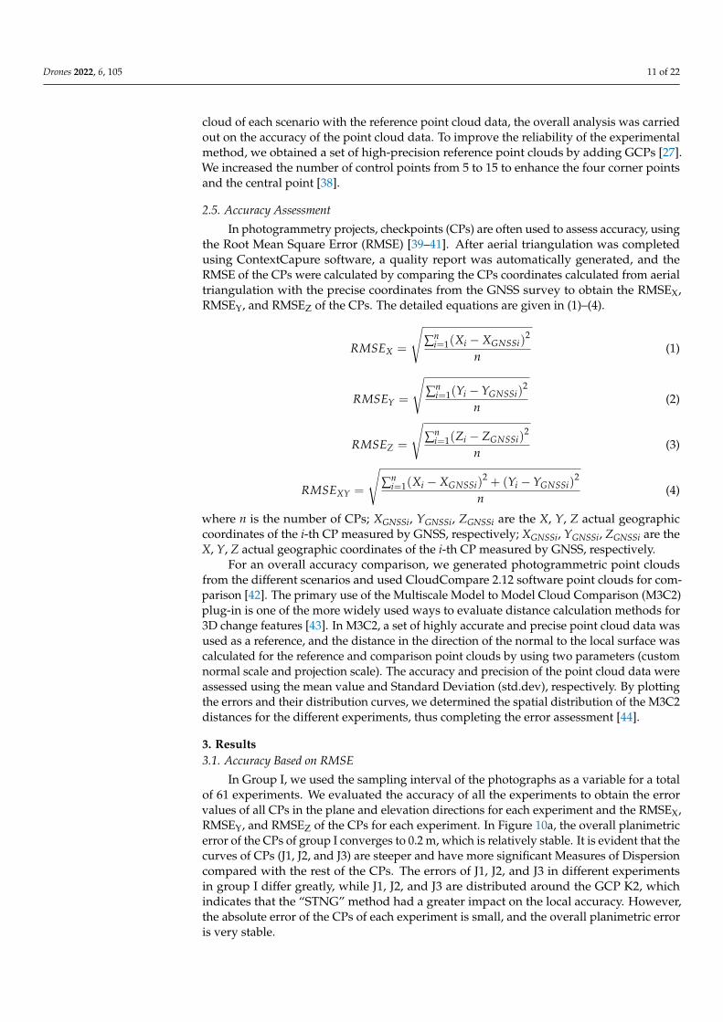
2.5. Accuracy Assessment In photogrammetry projects, checkpoints (CPs) are often used to assess accuracy, us-

ing the Root Mean Square Error (RMSE) [39–41]. After aerial triangulation was completed using ContextCapure software, a quality report was automatically generated, and the RMSE of the CPs were calculated by comparing the CPs coordinates calculated from aerial triangulation with the precise coordinates from the GNSS survey to obtain the RMSEX, RMSEY, and RMSEZ of the CPs. The detailed equations are given in (1)–(4).

𝑅𝑀𝑆𝐸 = ∑ (𝑋 − 𝑋 )𝑛 (1)

𝑅𝑀𝑆𝐸 = ∑ (𝑌 − 𝑌 )𝑛 (2)

𝑅𝑀𝑆𝐸 = ∑ (𝑍 − 𝑍 )𝑛 (3)

Figure 9. Set-up of three different spatial position scenarios: (a) heading angle interval α = 20◦;(b) heading angle interval α = 40◦; (c) heading angle interval α = 60◦. We defined the direction to benorth, with a heading angle starting at 0◦, and the UAV movement direction was clockwise.

A set of experimental data was selected from the results of Group I and Group II,respectively, together with the remaining experiments, including “NFP”, ”4 GCPs”, and“5 GCPs” for a total of five experiments. The photogrammetric point cloud model was gen-erated for each experiment, and the sampling distance of the point cloud was set to 0.1 m.

The point cloud analysis was carried out using the M3C2 plug-in of Cloud comparesoftware. The parameters were adjusted according to the system recommended values(Guess params), with a projection radius of 0.87 m, an initial value of 0.44 m, a step size of0.44 m, a final value of 1.74 m, and a calculation depth of 0.40 m. By comparing the point

Drones 2022, 6, 105 11 of 22

cloud of each scenario with the reference point cloud data, the overall analysis was carriedout on the accuracy of the point cloud data. To improve the reliability of the experimentalmethod, we obtained a set of high-precision reference point clouds by adding GCPs [27].We increased the number of control points from 5 to 15 to enhance the four corner pointsand the central point [38].

2.5. Accuracy Assessment

In photogrammetry projects, checkpoints (CPs) are often used to assess accuracy, usingthe Root Mean Square Error (RMSE) [39–41]. After aerial triangulation was completedusing ContextCapure software, a quality report was automatically generated, and theRMSE of the CPs were calculated by comparing the CPs coordinates calculated from aerialtriangulation with the precise coordinates from the GNSS survey to obtain the RMSEX,RMSEY, and RMSEZ of the CPs. The detailed equations are given in (1)–(4).

RMSEX =

√∑n

i=1(Xi − XGNSSi)2

n(1)

RMSEY =

√∑n

i=1(Yi −YGNSSi)2

n(2)

RMSEZ =

√∑n

i=1(Zi − ZGNSSi)2

n(3)

RMSEXY =

√∑n

i=1(Xi − XGNSSi)2 + (Yi −YGNSSi)

2

n(4)

where n is the number of CPs; XGNSSi, YGNSSi, ZGNSSi are the X, Y, Z actual geographiccoordinates of the i-th CP measured by GNSS, respectively; XGNSSi, YGNSSi, ZGNSSi are theX, Y, Z actual geographic coordinates of the i-th CP measured by GNSS, respectively.

For an overall accuracy comparison, we generated photogrammetric point cloudsfrom the different scenarios and used CloudCompare 2.12 software point clouds for com-parison [42]. The primary use of the Multiscale Model to Model Cloud Comparison (M3C2)plug-in is one of the more widely used ways to evaluate distance calculation methods for3D change features [43]. In M3C2, a set of highly accurate and precise point cloud data wasused as a reference, and the distance in the direction of the normal to the local surface wascalculated for the reference and comparison point clouds by using two parameters (customnormal scale and projection scale). The accuracy and precision of the point cloud data wereassessed using the mean value and Standard Deviation (std.dev), respectively. By plottingthe errors and their distribution curves, we determined the spatial distribution of the M3C2distances for the different experiments, thus completing the error assessment [44].

3. Results3.1. Accuracy Based on RMSE

In Group I, we used the sampling interval of the photographs as a variable for a totalof 61 experiments. We evaluated the accuracy of all the experiments to obtain the errorvalues of all CPs in the plane and elevation directions for each experiment and the RMSEX,RMSEY, and RMSEZ of the CPs for each experiment. In Figure 10a, the overall planimetricerror of the CPs of group I converges to 0.2 m, which is relatively stable. It is evident that thecurves of CPs (J1, J2, and J3) are steeper and have more significant Measures of Dispersioncompared with the rest of the CPs. The errors of J1, J2, and J3 in different experimentsin group I differ greatly, while J1, J2, and J3 are distributed around the GCP K2, whichindicates that the “STNG” method had a greater impact on the local accuracy. However,the absolute error of the CPs of each experiment is small, and the overall planimetric erroris very stable.

Drones 2022, 6, 105 12 of 22Drones 2022, 6, x FOR PEER REVIEW 14 of 24

(a)

(b)

Figure 10. Horizontal XY (a) and vertical Z (b) error distributions at CPs in group I. The abscissa represents the serial numbers of 61 different experiments (corresponding to Figure 7); the ordinate represents the error of the CPs, and each column of data represents the size of the error value of the 19 CPs in each experiment. The 19 CPs are distinguished by 19 colors, and the broken line represents the fluctuation of the error of the 19 CPs with the change of the experiment.

Figure 10 shows that the distribution of error values in the elevation direction is not as concentrated as the plane, and the overall convergence was −0.5 m~0.2 m. There are

0.00

0.02

0.04

0.06

0.08

0.10

0.12

0.14

0.16

0.18

0.20

1 2 3 4 5 6 7 8 9 10 11 12 13 14 15 16 17 18 19 20 21 22 23 24 25 26 27 28 29 30 31 32 33 34 35 36 37 38 39 40 41 42 43 44 45 46 47 48 49 50 51 52 53 54 55 56 57 58 59 60 61

Che

ck P

oint

Err

or_X

Y(m

)

"STNG" experiment number

j1 j2 j3 j4 j5 j6 j7 j8 j9 j10 j11 j12 j13 j14 j15 j16 j17 j18 j19

-0.90

-0.80

-0.70

-0.60

-0.50

-0.40

-0.30

-0.20

-0.10

0.00

0.10

0.20

1 2 3 4 5 6 7 8 9 10 11 12 13 14 15 16 17 18 19 20 21 22 23 24 25 26 27 28 29 30 31 32 33 34 35 36 37 38 39 40 41 42 43 44 45 46 47 48 49 50 51 52 53 54 55 56 57 58 59 60 61

Che

ck P

oint

Err

or_Z

(m)

"STNG" experiment number

J1 J2 J3 J4 J5 J6 J7 J8 J9 J10 J11 J12 J13 J14 J15 J16 J17 J18 J19

Figure 10. Horizontal XY (a) and vertical Z (b) error distributions at CPs in group I. The abscissarepresents the serial numbers of 61 different experiments (corresponding to Figure 7); the ordinaterepresents the error of the CPs, and each column of data represents the size of the error value of the19 CPs in each experiment. The 19 CPs are distinguished by 19 colors, and the broken line representsthe fluctuation of the error of the 19 CPs with the change of the experiment.

Drones 2022, 6, 105 13 of 22

Figure 10 shows that the distribution of error values in the elevation direction is notas concentrated as the plane, and the overall convergence was −0.5 m~0.2 m. There areapparent differences in the elevation errors between the different experiments in group I,which was unstable. The instability of CPs (J1, J2, J3, J4, and J10) is more pronounced, asthese 5 points were distributed around K2, further verifying that the “STNG” method has agreater impact on local accuracy. On the other hand, the crests indicate the convergenceof error values for the overall CPs of this experiment, and elevation errors were smaller.It can be found that the experiments in the case of full photo participation (experimentnumbers 1, 28, 41, 49, 54, 58, and 61) are at the wave crest in the group of seven differentsampling interval distances; this means that a uniform distribution of photographs within160 m according to the sampling interval has less error than a partial take of five, while thenumber of uniformly distributed photographs is greater compared to five (five photos for35 m sampling distance). Figure 11 represents the fitted curve between sampling intervaland CPs RMSE for these seven experiments. The results show that the effect of the samplinginterval on the CPs was significant, with the RMSE of the CPs gradually decreasing andthen stabilising as a power function relationship as the distance between the samplingintervals increases (regression coefficients R2 = 0.610, significance level p < 0.05). However,larger sampling intervals (40 m and above) would not satisfy the experimental conditions,which were limited by the flight height of the data itself.

Drones 2022, 6, x FOR PEER REVIEW 15 of 24

apparent differences in the elevation errors between the different experiments in group I, which was unstable. The instability of CPs (J1, J2, J3, J4, and J10) is more pronounced, as these 5 points were distributed around K2, further verifying that the “STNG” method has a greater impact on local accuracy. On the other hand, the crests indicate the convergence of error values for the overall CPs of this experiment, and elevation errors were smaller. It can be found that the experiments in the case of full photo participation (experiment numbers 1, 28, 41, 49, 54, 58, and 61) are at the wave crest in the group of seven different sampling interval distances; this means that a uniform distribution of photographs within 160 m according to the sampling interval has less error than a partial take of five, while the number of uniformly distributed photographs is greater compared to five (five photos for 35 m sampling distance). Figure 11 represents the fitted curve between sampling in-terval and CPs RMSE for these seven experiments. The results show that the effect of the sampling interval on the CPs was significant, with the RMSE of the CPs gradually de-creasing and then stabilising as a power function relationship as the distance between the sampling intervals increases (regression coefficients R2 = 0.610, significance level p < 0.05). However, larger sampling intervals (40 m and above) would not satisfy the experimental conditions, which were limited by the flight height of the data itself.

Figure 11. RMSEZ analysis of seven groups of experiments involving all photos at different distance intervals (calculated in MS Excel and IBM SPSS Statistics). The 5 m [5–160] measurement on the graph indicates that all photos (32 photos) with a sampling interval of 5 m in the interval 5–160 m participated in the experiment. The figure also shows the bounds of the CPs RMSEZ for 5 GCPs.

In order to determine how the accuracy varies with the spatial position of the photo-graph in the vertical direction, a correlation analysis was carried out on the “5 m” series of 26 experiments. The experiments are numbered 2–27 (Figure 7) (remove experiment number 16, which has a large outlier, RMSEZ = 0.0815 m). Figure 12 shows a significant correlation between the overall height of the five photographs and the CPs RMSEZ, with the RMSEZ showing a linear increase as the overall height of the photographs increases (regression coefficients R2 = 0.6434, Pearson coefficient of 0.811, significance level p < 0.001). The values in the graph are valid only for this study, as the errors depend on the sampling interval.

y = 0.289x-0.376

R² = 0.610

0.00

0.02

0.04

0.06

0.08

0.10

0.12

0.14

0.16

0.18

0.20

Che

ck P

oint

RM

SE(m

)

5GCPs RMSE=0.0877m

Figure 11. RMSEZ analysis of seven groups of experiments involving all photos at different distanceintervals (calculated in MS Excel and IBM SPSS Statistics). The 5 m [5–160] measurement on thegraph indicates that all photos (32 photos) with a sampling interval of 5 m in the interval 5–160 mparticipated in the experiment. The figure also shows the bounds of the CPs RMSEZ for 5 GCPs.

In order to determine how the accuracy varies with the spatial position of the photo-graph in the vertical direction, a correlation analysis was carried out on the “5 m” series of26 experiments. The experiments are numbered 2–27 (Figure 7) (remove experiment number16, which has a large outlier, RMSEZ = 0.0815 m). Figure 12 shows a significant correlationbetween the overall height of the five photographs and the CPs RMSEZ, with the RMSEZshowing a linear increase as the overall height of the photographs increases (regressioncoefficients R2 = 0.6434, Pearson coefficient of 0.811, significance level p < 0.001). The valuesin the graph are valid only for this study, as the errors depend on the sampling interval.

Drones 2022, 6, 105 14 of 22Drones 2022, 6, x FOR PEER REVIEW 16 of 24

Figure 12. Elevation error at the checkpoints as a function of the overall height value of the photo (calculated in MS Excel). The horizontal axis represents the maximum flight height in the photos of each experiment in the 5 m interval group (for example, the maximum flight height of the five pho-tos in the experiment number 2 is 160 m, and the experiment number 3 is 155 m), and the vertical axis is the RMSEZ of each experimental checkpoint.

The main focus of Group II was to investigate the effect of different flight altitudes and heading angle intervals on accuracy. In the nomenclature of the experiment, II_140 m_20° (18) indicates an “Oblique and Circle” of 18 photographs at a flight height of 140 m and a heading angle interval of 20°.

Table 4 shows the RMSE of the CPs for the different solutions of the “Oblique and Circle” method. Different schemes can meet the accuracy requirements of “5GCPs” (RMSEX = 70.40 mm, RMSEY = 53.90 mm, RMSEZ = 87.70 mm) in both horizontal and ele-vation directions, indicating the effectiveness and stability of the “Oblique and Circle” method. When the number of images was reduced to six, the overall accuracy does not change significantly, so we preferred to use six images. After comparison, the 140 m aerial height shows a higher elevation accuracy, with the best being at CPs RMSEZ = 75 mm.

Table 4. RMSE in the horizontal and elevation direction for different flight altitudes and different numbers of photographs using the “Oblique and Circle” method.

Experiment RMSEX (mm) RMSEY (mm) RMSEZ (mm) II_140m_20° (18) 70.70 51.80 77.90 II_140m_60° (6) 70.60 52.10 75.00

II_160m_20° (18) 71.10 51.10 87.30 II_160m_60° (6) 71.30 50.70 83.00

II_180m_20° (18) 70.80 50.80 74.30 II_180m_60° (6) 70.30 53.20 84.20

From the results of the above experiments, it can be concluded that the accuracy was better at a flight altitude of 140 m. Therefore, data with a flight altitude of 140 m was used to explore the effect of different spatial positions of the photographs on accuracy. The number of photographs was six, and three sets of experiments were designed (Figure 9). The results of the experiments are shown in Table 5. The errors show fluctuations as the relative spatial positions of the photographs vary. The smallest error is in experiment

y = 0.0015x + 0.0677R² = 0.6434

0.00

0.05

0.10

0.15

0.20

0.25

0.30

0.35

0.40

30 40 50 60 70 80 90 100 110 120 130 140 150 160

Che

ck P

oint

RM

SE_Z

(m)

Maximum flight altitude(m)

Figure 12. Elevation error at the checkpoints as a function of the overall height value of the photo(calculated in MS Excel). The horizontal axis represents the maximum flight height in the photos ofeach experiment in the 5 m interval group (for example, the maximum flight height of the five photosin the experiment number 2 is 160 m, and the experiment number 3 is 155 m), and the vertical axis isthe RMSEZ of each experimental checkpoint.

The main focus of Group II was to investigate the effect of different flight altitudesand heading angle intervals on accuracy. In the nomenclature of the experiment, II_140m_20◦ (18) indicates an “Oblique and Circle” of 18 photographs at a flight height of 140 mand a heading angle interval of 20◦.

Table 4 shows the RMSE of the CPs for the different solutions of the “Oblique andCircle” method. Different schemes can meet the accuracy requirements of “5GCPs”(RMSEX = 70.40 mm, RMSEY = 53.90 mm, RMSEZ = 87.70 mm) in both horizontal andelevation directions, indicating the effectiveness and stability of the “Oblique and Circle”method. When the number of images was reduced to six, the overall accuracy does notchange significantly, so we preferred to use six images. After comparison, the 140 m aerialheight shows a higher elevation accuracy, with the best being at CPs RMSEZ = 75 mm.

Table 4. RMSE in the horizontal and elevation direction for different flight altitudes and differentnumbers of photographs using the “Oblique and Circle” method.

Experiment RMSEX (mm) RMSEY (mm) RMSEZ (mm)

II_140m_20◦ (18) 70.70 51.80 77.90II_140m_60◦ (6) 70.60 52.10 75.00II_160m_20◦ (18) 71.10 51.10 87.30II_160m_60◦ (6) 71.30 50.70 83.00II_180m_20◦ (18) 70.80 50.80 74.30II_180m_60◦ (6) 70.30 53.20 84.20

From the results of the above experiments, it can be concluded that the accuracy wasbetter at a flight altitude of 140 m. Therefore, data with a flight altitude of 140 m was used toexplore the effect of different spatial positions of the photographs on accuracy. The numberof photographs was six, and three sets of experiments were designed (Figure 9). The resultsof the experiments are shown in Table 5. The errors show fluctuations as the relative spatialpositions of the photographs vary. The smallest error is in experiment II_140m_60◦ (6),

Drones 2022, 6, 105 15 of 22

representing a uniform distribution of images, with the heading angle of every two imagesdiffering by 60◦ and the RMSEZ being 75 mm. However, the RMSEZ for the rest of theexperiments was less than 87.70 mm (5 GCPs), which further validates the stability of the“Oblique and Circle” method.

Table 5. CPs RMSE of three distribution modes at 140 m altitude by the “Oblique and Circle” method.

Experiment RMSEX (mm) RMSEY (mm) RMSEZ (mm)

II_140m_60◦ (6) 70.60 52.10 75.00II_140m_20◦ (6) 71.00 51.90 79.80II_140m_40◦ (6) 70.50 52.50 86.00

Experiment I_54 and experiment II_140m_60◦ (6) were used as the representativeresults of group I and group II, respectively, and the accuracy was compared with “NFP”(using natural feature points as control points), “4 GCPs” (K2 point loss), and “5 GCPs”.From Figure 13, in the X-direction, the largest error was NFP with CPs RMSEX = 94.80 mm,followed by 4 GCPs, CPs RMSEX = 75 mm. The results show that adding a natural featurepoint as a GCP did not improve the accuracy but reduced it to some extent. The RMSEX ofExperiment I_54, Experiment II_140 m_60◦ (6), and 5 GCPs were 70.37 mm, 70.60 mm, and70.40 mm, respectively, and the accuracy in the X-direction remained the same for all three. Theerror distribution pattern in the Y-direction is consistent with that in the X-direction. It is verifiedthat our methods can meet the requirements of 5GCPs accuracy in the horizontal direction.

Drones 2022, 6, x FOR PEER REVIEW 17 of 24

II_140m_60° (6), representing a uniform distribution of images, with the heading angle of every two images differing by 60° and the RMSEZ being 75 mm. However, the RMSEZ for the rest of the experiments was less than 87.70 mm (5 GCPs), which further validates the stability of the “Oblique and Circle” method.

Table 5. CPs RMSE of three distribution modes at 140 m altitude by the “Oblique and Circle” method.

Experiment RMSEX (mm) RMSEY (mm) RMSEZ (mm) II_140m_60° (6) 70.60 52.10 75.00 II_140m_20° (6) 71.00 51.90 79.80 II_140m_40° (6) 70.50 52.50 86.00

Experiment I_54 and experiment II_140m_60° (6) were used as the representative re-sults of group I and group II, respectively, and the accuracy was compared with “NFP” (using natural feature points as control points), “4 GCPs” (K2 point loss), and “5 GCPs”. From Figure 13, in the X-direction, the largest error was NFP with CPs RMSEX = 94.80 mm, followed by 4 GCPs, CPs RMSEX = 75 mm. The results show that adding a natural feature point as a GCP did not improve the accuracy but reduced it to some extent. The RMSEX of Experiment I_54, Experiment II_140 m_60° (6), and 5 GCPs were 70.37 mm, 70.60 mm, and 70.40 mm, respectively, and the accuracy in the X-direction remained the same for all three. The error distribution pattern in the Y-direction is consistent with that in the X-direction. It is verified that our methods can meet the requirements of 5GCPs accuracy in the horizontal direction.

In the Z-direction of elevation, the four GCPs exhibited the largest error, with CPs RMSEZ = 145.10 mm being greater than the 5 GCPs (CPs RMSEZ = 87.70 mm), which indi-cates that the absence of a GCP has a greater impact on the overall elevation accuracy. The NFP solution RMSEZ was 104.40 mm, which is between 4 GCPs and 5 GCPs, indicating that the addition of a natural feature point can improve the overall accuracy to some extent, compared to the elevation accuracy of 4 GCPs, but cannot achieve the accuracy (5 GCPs). In contrast, both the “STNG” and the “Oblique and Circle” met the accuracy of the 5 GCPs with an CPs RMSEZ of 71.41 mm and 75.00 mm, respectively, to a certain extent, thus im-proving the elevation accuracy.

70.37 70.60

94.80

75.00 70.40

53.77 52.10

68.80 62.50

53.90

71.41 75.00

104.40

145.10

87.70

0.00

20.00

40.00

60.00

80.00

100.00

120.00

140.00

160.00

Ⅰ_54 Ⅱ_140m_60°（6） NSP 4GCPs 5GCPs

Che

ck P

oint

RM

SE(m

m)

Experiment name

RMSEX RMSEY RMSEZ

Figure 13. RMSE in the X-, Y- and Z-directions for the checkpoints of the five key scenarios.

In the Z-direction of elevation, the four GCPs exhibited the largest error, with CPsRMSEZ = 145.10 mm being greater than the 5 GCPs (CPs RMSEZ = 87.70 mm), whichindicates that the absence of a GCP has a greater impact on the overall elevation accuracy.The NFP solution RMSEZ was 104.40 mm, which is between 4 GCPs and 5 GCPs, indicatingthat the addition of a natural feature point can improve the overall accuracy to some extent,compared to the elevation accuracy of 4 GCPs, but cannot achieve the accuracy (5 GCPs).In contrast, both the “STNG” and the “Oblique and Circle” met the accuracy of the 5 GCPswith an CPs RMSEZ of 71.41 mm and 75.00 mm, respectively, to a certain extent, thusimproving the elevation accuracy.

Drones 2022, 6, 105 16 of 22

3.2. Point Cloud Evaluation Based on M3C2 Distance

The photogrammetric point cloud of the “15 GCPs” scheme was used as the ref-erence point cloud, and the M3C2 distance operation was performed with the abovefive sets of experimental point clouds respectively, to obtain the point cloud change re-sults (Figure 14). The comparative analysis shows that the”4 GCPs” (mean = −0.0409,std. dev = 0.1223) was greatly affected in terms of accuracy and precision compared to“5 GCPs” (mean = −0.0239, std. dev = 0.0666), and the use of natural feature point as a GCP(mean = −0.0320, std. dev = 0.0734) could improve the accuracy but failed to achieve the5 GCPs accuracy. When five additional images with different altitudes (I_54) were added(mean = 0.0040, std. dev = 0.0652), the accuracy greatly improved (Figure 14a). When fiveoblique-circle images (II_140 m_60◦ (6)) were added (mean = 0.0017, std. dev = 0.0694),the overall accuracy and precision improved significantly and were closer to that of the15 GCPs (Figure 14b).

Drones 2022, 6, x FOR PEER REVIEW 18 of 24

Figure 13. RMSE in the X-, Y- and Z-directions for the checkpoints of the five key scenarios.

3.2. Point Cloud Evaluation Based on M3C2 Distance The photogrammetric point cloud of the “15 GCPs” scheme was used as the reference

point cloud, and the M3C2 distance operation was performed with the above five sets of experimental point clouds respectively, to obtain the point cloud change results (Figure 14). The comparative analysis shows that the”4 GCPs” (mean = −0.0409, std. dev = 0.1223) was greatly affected in terms of accuracy and precision compared to “5 GCPs” (mean = −0.0239, std. dev = 0.0666), and the use of natural feature point as a GCP (mean = −0.0320, std. dev = 0.0734) could improve the accuracy but failed to achieve the 5 GCPs accuracy. When five additional images with different altitudes (I_56) were added (mean = 0.0040, std. dev = 0.0652), the accuracy greatly improved (Figure 14a). When five oblique-circle images (II_140 m_60° (6)) were added (mean = 0.0017, std. dev = 0.0694), the overall accu-racy and precision improved significantly and were closer to that of the 15 GCPs (Figure 14b).

When the GCP (K2) is lost, it significantly impacted the accuracy of the study area, especially around the anomalous GCP and houses, which could be improved by the “STNG” and “Oblique and Circle” solution, and was significantly better than the use of natural feature points (Figure 14c).

(a)

(b)

Figure 14. Cont.

Drones 2022, 6, 105 17 of 22

Drones 2022, 6, x FOR PEER REVIEW 19 of 24

(c)

(d)

(e)

Figure 14. Different scenarios M3C2 Distances (in m). Square black dots for GCPs, triangular black dots for natural feature points. (a) 15GCPs-I_56; mean = 0.0040, std. dev = 0.0652, (b) 15 GCPs-II_140 m_60° (6); mean = 0.0017, std. dev = 0.0694, (c) 15 GCPs-Natural Feature Point; mean = −0.0320, std. dev = 0.0734, (d) 15 GCPs-4 GCPs; mean = −0.0409, std. dev = 0.1223, (e) 15 GCPs-5 GCPs; mean = −0.0239, std. dev = 0.0666.

Figure 14. Different scenarios M3C2 Distances (in m). Square black dots for GCPs, triangular blackdots for natural feature points. (a) 15GCPs-I_54; mean = 0.0040, std. dev = 0.0652, (b) 15 GCPs-II_140m_60◦ (6); mean = 0.0017, std. dev = 0.0694, (c) 15 GCPs-Natural Feature Point; mean = −0.0320,std. dev = 0.0734, (d) 15 GCPs-4 GCPs; mean = −0.0409, std. dev = 0.1223, (e) 15 GCPs-5 GCPs;mean = −0.0239, std. dev = 0.0666.

When the GCP (K2) is lost, it significantly impacted the accuracy of the study area,especially around the anomalous GCP and houses, which could be improved by the “STNG”and “Oblique and Circle” solution, and was significantly better than the use of naturalfeature points (Figure 14c).

Drones 2022, 6, 105 18 of 22

4. Discussion

We placed GCPs at each of the four corners and central points within the approximatelyrectangular study area, and this approach was feasible. Both Rangel et al. [45] and PatricioMartínez-Carricondo et al. [46] argued that a uniform distribution around the experimentalarea and the addition of uniformly distributed GCPs in the middle of the experimentalarea can improve the elevation accuracy. The errors introduced when a corner point K2 islost are significant, especially in elevation, with the RMSEZ of the CPs reaching 145.10 mmcompared to the 5 GCPs RMSEZ = 87.70 mm. Therefore, the quality of the photographsafter the loss of a GCP should be questioned and should not be used directly.

The anomalies in GCPs have rarely been discussed in previous studies. The generalmethod of a “natural feature point” has limitations and is very dependent on the qualityof the natural feature points and the subjective judgement of the data processor. It wasfound that when natural feature points were used as control points (NFP scheme), the errorin the elevation direction of the CPs reached 104.40 mm, which is not possible to achievethe accuracy of 5 GCPs. There is a significant increase in error in the horizontal direction,with the CPs RMSEX reaching 94.80 mm compared to the 5 GCPs checkpoints RMSEX of70.40 mm, further verifying that NFP is unable to achieve the 5 GCPs’ accuracy in boththe horizontal and elevation directions. Such instability is determined by the quality ofthe natural feature point— its actual position is not easy to find on the aerial images andis often met with some deviation. Francisco-Javier Mesas–Carrascosa’s study shows thatinstead of using well-defined artificial checkpoints, the use of natural feature points in thestudy area as checkpoints would increase the checkpoint RMSE from a GSD of 3.7 times toa GSD of five times [47].

The idea of the “STNG” method is to improve the ground resolution of the areaaround the GCP by progressively taking additional images downwards and fusing themwith the nadiral images, thus improving the accuracy. Quoc Long et al. [48] mentioned thatincreasing the ground resolution by reducing the flight altitude of the UAV could improvethe accuracy, and Agüera-Vega et al. [38] showed that the effect of GSD on elevationaccuracy was significant. In contrast, the effect on planimetric accuracy was smaller.

It was found that the “STNG” showed high stability in the horizontal direction butless stability in the elevation direction. The first experiment of each group representsthe best case for each group, all the images in each group are involved, and their spa-tial locations are shown in Figure 7. As the interval between adjacent photos increased,the elevation accuracy showed a nonlinear trend of gradual improvement and stability(regression coefficients R2 = 0.610, significance level p < 0.05), which is consistent withthe accuracy of “5 GCPs”, indicating that the “STNG” is feasible. The best solution is toset the sampling interval as 25 m (I_54), where all seven images were involved and theRMSEX = 70.37 mm, RMSEY = 53.77 mm, RMSEZ = 71.41 mm of the CPs. The RMSEZof the CPs of the sampling interval of 30 m (I_58) and 35 m (I_61) were 88.61 mm and73.85 mm—both of which met the 5 GCP’s accuracy requirements. Therefore, we suggestthat in the actual operation, the sampling interval D should be determined with referenceto the nadiral flight altitude ((H + ∆h)/7 ≤ D ≤ (H + ∆h)/5, where H is the nadiral flightaltitude and ∆h is the difference between the altitude of the nadiral take-off point and thealtitude of the anomalous GCP).

In experiments with a sampling interval of 5 m, we found a linear trend in the accuracyof the data with decreasing photo height (regression coefficients R2 = 0.6434, significancelevel p < 0.001). This observation will need to be verified in further studies.

A total of six experiments were set up in Group II to verify the influence of altitudeand number of photographs on the accuracy, and three experiments were set up to verifythe influence of different spatial positions of photographs at the same altitude on accuracy.The results show that the accuracy of the 5 GCPs can be achieved at different flight altitudes,indicating that the “Oblique and Circle” method has high stability. The highest elevationaccuracy was demonstrated at an altitude of 140 m. The difference between the accuracyof 18 additional images and six images is not significant, so using six images was a better

Drones 2022, 6, 105 19 of 22

choice. When the spatial position of six images was evenly distributed, and the headingangles of different images were spaced 60◦ apart, which is more accurate. The horizontalerror of the above experiment is about one-to-two times the GSD, and the elevation error isabout two-to-three times the GSD, which satisfies the general law of photogrammetry [49].

By using the “Oblique and Circle” method, there is a clear tendency to improveaccuracy in the elevation direction further. The RMSEZ of the CPs of the II_140m_60◦ (6)experiment is 75.00 mm, which is about 10 mm higher elevation accuracy than the 5 GCPs.Wackrow et al. [50] suggested that the angle between homologous rays could be increasedby introducing oblique images in the nadiral dataset, thus reducing systematic errors.Bi et al. [51], Harwin et al. [52], and Štroner et al. [25] have shown that adding additionaloblique images to the nadiral images can improve the accuracy of the results and increasethe elevation accuracy. Sanz-Ablanedo et al. [53] showed that square POI flights, where thecamera angle is always aligned with the centre of the region of interest, produce a smallersystematic error. Therefore, we believe that the “Oblique and Circle” method is valid andis valuable for further research.

The M3C2 point cloud comparison confirms our viewpoint as well. Using the “STNG”and “Oblique and Circle” methods can improve the elevation accuracy to a certain extentwhile still meeting the 5 GCPs’ accuracy. The “Oblique and Circle” method provides thehighest elevation accuracy and is more stable. The “natural feature point” method has asignificant local error (Figure 14c), and the overall accuracy is not as good as required.

In UAS, the height above the ground level can be measured based on barometersensors. The DJI Phantom 4 Pro UAV used in this study has a vertical positioning accuracyof ±0.5 m, which means that height deviations at the decimetre level may occur duringdata acquisition and that the centimetre level (or smaller) positioning accuracy cannot beaccomplished [54]. However, the two methods are experimentally compatible, and thedecimetre-level positioning errors have less impact on the two methods. Therefore, thevertical positioning errors of the UAV itself can be ignored when using the methods.

At the same time, the limitations of fixed-wing UAVs make it challenging to use themethod proposed in this paper to collect images. Therefore, the fusion of images usingdifferent camera sensors is proposed, such as using a more flexible multirotor UAV tocomplement images; this will be the next stage of our research.

5. Conclusions

In this paper, two different solutions based on ground control point anomalies wereput forward, and the optimum of which was verified. By adopting the “5 GCPs” asthe reference project and the “NFP” method as the comparison solution, the followingconclusions can be drawn.

It is not easy to find natural feature points that meet the requirements outside urbanareas. The location of the feature points in the image depends on the subjective judgmentof professionals with a large error caused by “human factors”. For this reason, it is notrecommended that “natural features” be the preferred option for aerial photogrammetrywhen high accuracy is required.

In practical projects, only when horizontal accuracy is required, can our proposed“STNG” and “Oblique and Circle” methods meet the accuracy requirements. The “NFP”demonstrates that neither the horizontal nor the elevation direction can meet the require-ments of the 5 GCPs’ accuracy. The “STNG” method is simple and easy to use, so it isrecommended. When using the “STNG” method, the spacing between the adjacent imagesis D ((H + ∆h)/7 ≤ D ≤ (H+ ∆h)/5, where H is the nadiral flight altitude, ∆h is the differ-ence between the elevation of the nadiral take-off point and the elevation of the anomalyGCP, and the number of photographs must not be less than 5.).

When elevation accuracy is considered, the “Oblique and Circle” method has higherstability and meets the accuracy requirements. In the horizontal direction, the accuracy ismaintained and consistent with the data´s accuracy from the 5 GCPs. There is a tendencyto improve the accuracy further in the elevation direction. When using the “Oblique and

Drones 2022, 6, 105 20 of 22

Circle” method, the accuracy requirements can be met by keeping the flight height thesame as the flight height of the nadiral. To improve the elevation accuracy, the flightheight can be reduced by a small amount, e.g., about 20 m in the experiment of this paper.At the same time, the selection of photographs should be evenly distributed around theentire circumference, and the results are better when the heading angle is 60◦. In sum, the“Oblique and Circle” method is highly effective when the GCPs are anomalous.

Author Contributions: Conceptualization, J.Y. and X.L.; methodology, X.L. and J.Y.; formal analysis,X.L., L.Z. and J.W.; investigation, X.L., L.Z., J.Y. and J.W.; Resources, J.Y. and L.L.; writing—originaldraft preparation, X.L. and J.Y.; writing—review and editing, J.Y.; visualization, X.L. and T.M.;supervision, J.Y. and L.L.; funding acquisition, L.L. All authors have read and agreed to the publishedversion of the manuscript.

Funding: This work was supported by the Strategic Priority Research Program of the ChineseAcademy of Sciences (Grant No. XDA19030504).

Institutional Review Board Statement: Not applicable.

Informed Consent Statement: Not applicable.

Data Availability Statement: Not applicable.

Conflicts of Interest: The authors declare no conflict of interest.

References1. Šafár, V.; Potucková, M.; Karas, J.; Tlustý, J.; Štefanová, E.; Jancovic, M.; Cígler Žofková, D. The Use of UAV in Cadastral Mapping

of the Czech Republic. ISPRS Int. J. Geo-Inf. 2021, 10, 380. [CrossRef]2. Puniach, E.; Bieda, A.; Cwiakała, P.; Kwartnik-Pruc, A.; Parzych, P. Use of Unmanned Aerial Vehicles (UAVs) for Updating

Farmland Cadastral Data in Areas Subject to Landslides. ISPRS Int. J. Geo-Inf. 2018, 7, 331. [CrossRef]3. Chio, S.-H.; Chiang, C.-C. Feasibility Study Using UAV Aerial Photogrammetry for a Boundary Verification Survey of a Digitalized

Cadastral Area in an Urban City of Taiwan. Remote Sens. 2020, 12, 1682. [CrossRef]4. Alexiou, S.; Deligiannakis, G.; Pallikarakis, A.; Papanikolaou, I.; Psomiadis, E.; Reicherter, K. Comparing High Accuracy t-LiDAR

and UAV-SfM Derived Point Clouds for Geomorphological Change Detection. ISPRS Int. J. Geo-Inf. 2021, 10, 367. [CrossRef]5. De Marco, J.; Maset, E.; Cucchiaro, S.; Beinat, A.; Cazorzi, F. Assessing Repeatability and Reproducibility of Structure-from-Motion

Photogrammetry for 3D Terrain Mapping of Riverbeds. Remote Sens. 2021, 13, 2572. [CrossRef]6. Kyriou, A.; Nikolakopoulos, K.; Koukouvelas, I. How Image Acquisition Geometry of UAV Campaigns Affects the Derived

Products and Their Accuracy in Areas with Complex Geomorphology. ISPRS Int. J. Geo-Inf. 2021, 10, 408. [CrossRef]7. Bakirman, T.; Bayram, B.; Akpinar, B.; Karabulut, M.F.; Bayrak, O.C.; Yigitoglu, A.; Seker, D.Z. Implementation of Ultra-Light

UAV Systems for Cultural Heritage Documentation. J. Cult. Herit. 2020, 44, 174–184. [CrossRef]8. Berrett, B.E.; Vernon, C.A.; Beckstrand, H.; Pollei, M.; Markert, K.; Franke, K.W.; Hedengren, J.D. Large-Scale Reality Modeling

of a University Campus Using Combined UAV and Terrestrial Photogrammetry for Historical Preservation and Practical Use.Drones 2021, 5, 136. [CrossRef]

9. Teppati Losè, L.; Chiabrando, F.; Giulio Tonolo, F. Documentation of Complex Environments Using 360◦ Cameras. The SantaMarta Belltower in Montanaro. Remote Sens. 2021, 13, 3633. [CrossRef]

10. Fraser, B.T.; Congalton, R.G. Estimating Primary Forest Attributes and Rare Community Characteristics Using Unmanned AerialSystems (UAS): An Enrichment of Conventional Forest Inventories. Remote Sens. 2021, 13, 2971. [CrossRef]

11. Malachy, N.; Zadak, I.; Rozenstein, O. Comparing Methods to Extract Crop Height and Estimate Crop Coefficient from UAVImagery Using Structure from Motion. Remote Sens. 2022, 14, 810. [CrossRef]

12. Pagliai, A.; Ammoniaci, M.; Sarri, D.; Lisci, R.; Perria, R.; Vieri, M.; D’Arcangelo, M.E.M.; Storchi, P.; Kartsiotis, S.-P. Comparison ofAerial and Ground 3D Point Clouds for Canopy Size Assessment in Precision Viticulture. Remote Sens. 2022, 14, 1145. [CrossRef]

13. Santana, L.S.; Ferraz, G.A.e.S.; Marin, D.B.; Faria, R.d.O.; Santana, M.S.; Rossi, G.; Palchetti, E. Digital Terrain Modelling byRemotely Piloted Aircraft: Optimization and Geometric Uncertainties in Precision Coffee Growing Projects. Remote Sens. 2022,14, 911. [CrossRef]

14. Albeaino, G.; Gheisari, M. Trends, benefits, and barriers of unmanned aerial systems in the construction industry: A survey studyin the United States. J. Inf. Technol. Constr. 2021, 26, 84–111. [CrossRef]

15. Esposito, G.; Mastrorocco, G.; Salvini, R.; Oliveti, M.; Starita, P. Application of UAV Photogrammetry for the Multi-TemporalEstimation of Surface Extent and Volumetric Excavation in the Sa Pigada Bianca Open-Pit Mine, Sardinia, Italy. Environ. Earth Sci.2017, 76, 1–16. [CrossRef]

16. Hammad, A.; da Costa, B.; Soares, C.; Haddad, A. The Use of Unmanned Aerial Vehicles for Dynamic Site Layout Planning inLarge-Scale Construction Projects. Build 2021, 11, 602. [CrossRef]

Drones 2022, 6, 105 21 of 22

17. Lee, S.B.; Song, M.; Kim, S.; Won, J.-H. Change Monitoring at Expressway Infrastructure Construction Sites Using Drone. Sens.Mater. 2020, 32, 3923–3933. [CrossRef]

18. Rizo-Maestre, C.; González-Avilés, Á.; Galiano-Garrigós, A.; Andújar-Montoya, M.D.; Puchol-García, J.A. UAV + BIM: Incor-poration of Photogrammetric Techniques in Architectural Projects with Building Information Modeling Versus Classical WorkProcesses. Remote Sens. 2020, 12, 2329. [CrossRef]

19. Bolkas, D. Assessment of GCP Number and Separation Distance for Small UAS Surveys with and without GNSS-PPK Positioning.J. Surv. Eng. 2019, 145, 04019007. [CrossRef]

20. Hugenholtz, C.; Brown, O.; Walker, J.; Barchyn, T.; Nesbit, P.; Kucharczyk, M.; Myshak, S. Spatial Accuracy of UAV-DerivedOrthoimagery and Topography: Comparing Photogrammetric Models Processed with Direct Geo-Referencing and GroundControl Points. Geomatica 2016, 70, 21–30. [CrossRef]

21. Fazeli, H.; Samadzadegan, F.; Dadrasjavan, F. Evaluating the Potential of Rtk-Uav for Automatic Point Cloud Generation in 3dRapid Mapping. ISPRS—Int. Arch. Photogramm. Remote Sens. Spat. Inf. Sci. 2016, XLI-B6, 221–226. [CrossRef]

22. Forlani, G.; Dall’Asta, E.; Diotri, F.; Cella, U.M.d.; Roncella, R.; Santise, M. Quality Assessment of DSMs Produced from UAVFlights Georeferenced with On-Board RTK Positioning. Remote Sens. 2018, 10, 311. [CrossRef]

23. Benassi, F.; Dall’Asta, E.; Diotri, F.; Forlani, G.; Morra di Cella, U.; Roncella, R.; Santise, M. Testing Accuracy and Repeatability ofUAV Blocks Oriented with GNSS-Supported Aerial Triangulation. Remote Sens. 2017, 9, 172. [CrossRef]

24. Taddia, Y.; Stecchi, F.; Pellegrinelli, A. Coastal Mapping Using DJI Phantom 4 RTK in Post-Processing Kinematic Mode. Drones2020, 4, 9. [CrossRef]

25. Štroner, M.; Urban, R.; Seidl, J.; Reindl, T.; Broucek, J. Photogrammetry Using UAV-Mounted GNSS RTK: GeoreferencingStrategies without GCPs. Remote Sens. 2021, 13, 1336. [CrossRef]

26. Teppati Losè, L.; Chiabrando, F.; Giulio Tonolo, F. Boosting the Timeliness of UAV Large Scale Mapping. Direct GeoreferencingApproaches: Operational Strategies and Best Practices. ISPRS Int. J. Geo-Inf. 2020, 9, 578. [CrossRef]

27. James, M.R.; Robson, S. Mitigating systematic error in topographic models derived from UAV and ground-based image networks.Earth Surf. Processes Landf. 2014, 39, 1413–1420. [CrossRef]

28. Oniga, V.-E.; Breaban, A.-I.; Pfeifer, N.; Chirila, C. Determining the Suitable Number of Ground Control Points for UAS ImagesGeoreferencing by Varying Number and Spatial Distribution. Remote Sens. 2020, 12, 876. [CrossRef]

29. Sanz-Ablanedo, E.; Chandler, J.; Rodríguez-Pérez, J.; Ordóñez, C. Accuracy of Unmanned Aerial Vehicle (UAV) and SfMPhotogrammetry Survey as a Function of the Number and Location of Ground Control Points Used. Remote Sens. 2018, 10, 1606.[CrossRef]

30. Ferrer-González, E.; Agüera-Vega, F.; Carvajal-Ramírez, F.; Martínez-Carricondo, P. UAV Photogrammetry Accuracy Assessmentfor Corridor Mapping Based on the Number and Distribution of Ground Control Points. Remote Sens. 2020, 12, 2447. [CrossRef]

31. Liu, X.; Lian, X.; Yang, W.; Wang, F.; Han, Y.; Zhang, Y. Accuracy Assessment of a UAV Direct Georeferencing Method and Impactof the Configuration of Ground Control Points. Drones 2022, 6, 30. [CrossRef]

32. Ulvi, A. The Effect of the Distribution and Numbers of Ground Control Points on the Precision of Producing Orthophoto Mapswith an Unmanned Aerial Vehicle. J. Asian Archit. Build. Eng. 2021, 20, 806–817. [CrossRef]

33. Boon, M.A.; Drijfhout, A.P.; Tesfamichael, S. Comparison of a Fixed-Wing and Multi-Rotor Uav for Environmental MappingApplications: A Case Study. Int. Arch. Photogramm. Remote Sens. Spat. Inf. Sci. 2017, XLII-2/W6, 47–54. [CrossRef]

34. Reshetyuk, Y.; Mårtensson, S.-G. Generation of Highly Accurate Digital Elevation Models with Unmanned Aerial Vehicles.Photogramm. Rec. 2016, 31, 143–165. [CrossRef]

35. Context Capture 4.4.10. Available online: https://www.bentley.com/en/products/brands/contextcapture (accessed on19 February 2022).

36. Forsmoo, J.; Anderson, K.; Macleod, C.J.; Wilkinson, M.E.; DeBell, L.; Brazier, R.E. Structure from Motion Photogrammetry inEcology: Does the Choice of Software Matter? Ecol. Evol. 2019, 9, 12964–12979. [CrossRef] [PubMed]

37. Manyoky, M.; Theiler, P.; Steudler, D.; Eisenbeiss, H. Unmanned Aerial Vehicle in Cadastral Applications. The InternationalArchives of the Photogrammetry. Remote Sens. Spat. Inf. Sci. 2012, XXXVIII-1/C22, 57–62. [CrossRef]

38. Agüera-Vega, F.; Carvajal-Ramírez, F.; Martínez-Carricondo, P. Assessment of Photogrammetric Mapping Accuracy Based onVariation Ground Control Points Number Using Unmanned Aerial Vehicle. Measurement 2017, 98, 221–227. [CrossRef]

39. Rabah, M.; Basiouny, M.; Ghanem, E.; Elhadary, A. Using RTK and VRS in Direct Geo-Referencing of the UAV Imagery. NRIAG J.Astron. Geophys. 2019, 7, 220–226. [CrossRef]

40. Gerke, M.; Przybilla, H.J. Accuracy Analysis of Photogrammetric UAV Image Blocks: Influence of Onboard RTK-GNSS and CrossFlight Patterns. Photogramm. Fernerkund. Geoinf. (PFG) 2016, 1, 17–30. [CrossRef]

41. Lalak, M.; Wierzbicki, D.; Kedzierski, M. Methodology of Processing Single-Strip Blocks of Imagery with Reduction andOptimization Number of Ground Control Points in UAV Photogrammetry. Remote Sens. 2020, 12, 3336. [CrossRef]

42. CloudCompare v2.12. Available online: https://www.danielgm.net/cc/ (accessed on 19 February 2022).43. DiFrancesco, P.-M.; Bonneau, D.; Hutchinson, D.J. The Implications of M3C2 Projection Diameter on 3D Semi-Automated Rockfall

Extraction from Sequential Terrestrial Laser Scanning Point Clouds. Remote Sens. 2020, 12, 1885. [CrossRef]44. James, M.R.; Robson, S.; Smith, M.W. 3-D Uncertainty-Based Topographic Change Detection with Structure-From-Motion

Photogrammetry: Precision Maps for Ground Control and Directly Georeferenced Surveys. Earth Surf. Processes Landf. 2017, 42,1769–1788. [CrossRef]

Drones 2022, 6, 105 22 of 22

45. Rangel, J.M.G.; Gonçalves, G.R.; Pérez, J.A. The Impact of Number and Spatial Distribution of GCPs on the Positional Accuracyof Geospatial Products Derived from Low-Cost UASs. Int. J. Remote Sens. 2018, 39, 7154–7171. [CrossRef]

46. Martínez-Carricondo, P.; Agüera-Vega, F.; Carvajal-Ramírez, F.; Mesas-Carrascosa, F.-J.; García-Ferrer, A.; Pérez-Porras, F.-J.Assessment of UAV-Photogrammetric Mapping Accuracy Based on Variation of Ground Control Points. Int. J. Appl. Earth Obs.Geoinf. 2018, 72, 1–10. [CrossRef]

47. Mesas-Carrascosa, F.J.; Notario Garcia, M.D.; Merono de Larriva, J.E.; Garcia-Ferrer, A. An Analysis of the Influence of FlightParameters in the Generation of Unmanned Aerial Vehicle (UAV) Orthomosaicks to Survey Archaeological Areas. Sensors 2016,16, 1838. [CrossRef]

48. Quoc Long, N.; Goyal, R.; Khac Luyen, B.; Van Canh, L.; Xuan Cuong, C.; Van Chung, P.; Ngoc Quy, B.; Bui, X.-N. Influence ofFlight Height on The Accuracy of UAV Derived Digital Elevation Model at Complex Terrain. Inzynieria Miner. 2020, 1, 179–186.[CrossRef]

49. Casella, V.; Chiabrando, F.; Franzini, M.; Manzino, A.M. Accuracy Assessment of a UAV Block by Different Software Packages,Processing Schemes and Validation Strategies. ISPRS Int. J. Geo-Inf. 2020, 9, 164. [CrossRef]

50. Wackrow, R.; Chandler, J.H. Minimising Systematic Error Surfaces in Digital Elevation Models Using Oblique ConvergentImagery. Photogramm. Rec. 2011, 26, 16–31. [CrossRef]

51. Bi, R.; Gan, S.; Yuan, X.; Li, R.; Gao, S.; Luo, W.; Hu, L. Studies on Three-Dimensional (3D) Accuracy Optimization andRepeatability of UAV in Complex Pit-Rim Landforms as Assisted by Oblique Imaging and RTK Positioning. Sensors 2021, 21, 8109.[CrossRef]

52. Harwin, S.; Lucieer, A.; Osborn, J. The Impact of the Calibration Method on the Accuracy of Point Clouds Derived UsingUnmanned Aerial Vehicle Multi-View Stereopsis. Remote Sens. 2015, 7, 11933–11953. [CrossRef]

53. Sanz-Ablanedo, E.; Chandler, J.H.; Ballesteros-Pérez, P.; Rodríguez-Pérez, J.R. Reducing systematic dome errors in digitalelevation models through better UAV flight design. Earth Surf. Processes Landf. 2020, 45, 2134–2147. [CrossRef]

54. DJI Phantom 4 Pro. Available online: https://www.dji.com/phantom-4-pro/info#specs (accessed on 19 February 2022).