New Methodology to Model Metal Chemistry at High ...
200
New Methodology to Model Metal Chemistry at High Temperature by Mary Elizabeth Wagner S.B., Massachusetts Institute of Technology (2016) Submitted to the Department of Materials Science and Engineering in Partial Fulfillment of the Requirements for the Degree of Doctor of Science at the MASSACHUSETTS INSTITUTE OF TECHNOLOGY June 2021 ©2021 Massachusetts Institute of Technology. All rights reserved. Signature of Author ............................................................................ Department of Materials Science and Engineering May 12, 2021 Certified by .................................................................................... Antoine Allanore Associate Professor of Metallurgy Thesis Supervisor Accepted by .................................................................................... Frances M. Ross Chair Departmental Committee on Graduate Studies
-
Upload
khangminh22 -
Category
Documents
-
view
0 -
download
0
Transcript of New Methodology to Model Metal Chemistry at High ...

New Methodology to Model Metal Chemistry at High
Temperature
by
Mary Elizabeth Wagner
S.B., Massachusetts Institute of Technology (2016)
Submitted to the Department of Materials Science and Engineeringin Partial Fulfillment of the Requirements for the Degree of
Doctor of Science
at the
MASSACHUSETTS INSTITUTE OF TECHNOLOGY
June 2021
©2021 Massachusetts Institute of Technology. All rights reserved.
Signature of Author . . . . . . . . . . . . . . . . . . . . . . . . . . . . . . . . . . . . . . . . . . . . . . . . . . . . . . . . . . . . . . . . . . . . . . . . . . . .
Department of Materials Science and EngineeringMay 12, 2021
Certified by . . . . . . . . . . . . . . . . . . . . . . . . . . . . . . . . . . . . . . . . . . . . . . . . . . . . . . . . . . . . . . . . . . . . . . . . . . . . . . . . . . . .
Antoine AllanoreAssociate Professor of Metallurgy
Thesis Supervisor
Accepted by . . . . . . . . . . . . . . . . . . . . . . . . . . . . . . . . . . . . . . . . . . . . . . . . . . . . . . . . . . . . . . . . . . . . . . . . . . . . . . . . . . . .
Frances M. RossChair
Departmental Committee on Graduate Studies

Abstract
There is currently a lack of ability to predict which species will be reduced at the cathode and
what purity will be achieved during metal electrodeposition. Problems related to co-deposition
and contamination are usually avoided by using selective aqueous electrolytes or pre-purifying
feedstock. However, these approaches are not always possible, particularly when developing novel,
high temperature electrochemical processes where there is little experimental information about
the electrolyte. In addition, present thermodynamic modeling methods fall short of their ability
to accurately predict the properties of the multicomponent, high temperature solutions commonly
used for electrolytes. In absence of meaningful models and sufficient data, the standard state
electrochemical potential is often used as a metric to determine which reduction reaction will
dominate. However, this approach assumes every species in the electrolyte acts as if it were a pure
species, and does not accurately reflect true electrochemical behavior.
Herein, a new approach to modeling electrolytes is developed. By examining liquid solutions
in a traditional chemical thermodynamic framework, and using this as a foundation for combining
targeted experiments with calculated Gibbs energy data, deeper insights into the role of electrolytes
on cell behavior can be obtained. A quantitative link between the activity of the electrolyte
and the cathode composition is modeled. In order to expand the utility of the model, a new
reference state for activity has been derived, specifically suited to the unique challenges of electrolyte
thermodynamics. This model was tested against experimental data for several case study systems
and performed well at predicting electrochemical behavior. Activity measured relative to the new
reference state accurately informed on thermodynamic phenomena. Use of the model on systems
with limited data enabled efficient design of new electrochemical processes.
3

4

To my grandfather,
Joseph Gregory Leija
5

6

Acknowledgements
This thesis would not have been possible without the guidance and support of many. I would
especially like to acknowledge Professor Allanore, who has been my research supervisor since Jan-
uary 2013, when I joined the laboratory as an undergraduate researcher. My time in your group has
shaped me into who I am today, both scientifically and personally, and graduation is a bittersweet
moment. When I began my research with you, I was a particularly poor student in thermody-
namics. Thank you for all your time and patience over the years teaching me the subject, and for
always pushing me to improve myself. I would also like to thank you for your mentorship over the
past 8 and a half years, and for all of our illuminating discussions in that time.
I would also like to thank and acknowledge Professor Sadoway and Professor Olivetti for not
only serving on my thesis committee, but also for the outstanding guidance you both have given
me during my time at MIT. Professor Sadoway, it was on your suggestion that I first joined the
Allanore Group, and in the time since you have provided invaluable advice as if I were your own
student, on subjects as narrow as immediate research problems to as broad as philosophical outlook.
Professor Olivetti, you have been a crucial mentor, helping me ground my work in sustainability
and encouraging me not to lose sight of those goals.
A very special thank you is in order for Professor Carter, who has also mentored me as if I were
his own student. You not only taught me the fundamentals of materials computation that made
this thesis possible, but you have also been a constant source of positivity and support. Thank you
also to Professor Morita, for always being at the ready with thermodynamic advice, and Professor
Fukunaka, for all of your help in successfully navigating conferences, as well as for hosting me
during my time in Japan.
7
To the Allanore Group members: I want to thank you for eight years of camaraderie. You have
always been there when I needed it the most, from midnight equipment repairs, to giving your
honest feedback on my work, to helping me take much-needed breaks from the lab. I would also
like to acknowledge the DMSE staff at large, especially Angelita Mireles and Mike Tarkanian, for
the countless hours you put in helping me and everyone else succeed at MIT.
Gianluca, the story of this thesis cannot be told without your companionship. We have gone
through every step of our doctorates together since we met as first years in September 2016:
studying for quals, defining our research, and now writing our theses. Thank you for always being
there for me through the highs and lows of this journey, and for the sheer joy you bring me every
day of our life together. I love you.
Thank you also to my family, especially my parents, Cynthia and Robert, and my siblings,
Mikey and Katey. I know I can always count on you no matter what, and I am forever grateful for
that. Thank you for always reminding me to keep things in perspective, and for the support and
advice you have given every step of the way. After 9 years, I’m finally graduating “college”.
Finally, I would like to thank my grandfather, Joseph Leija, to whom this thesis is dedicated.
You have given me the values, determination, and work ethic that guide me in everything I do. It
was when you were helping me recover from my foot surgery that I first derived the models that
would become the core of this work. It is impossible for me to look at the equations in this thesis
without thinking of you, and smiling.
8

Contents
Abstract 3
Acknlowledgements 7
List of Figures 20
List of Tables 21
1 Introduction 23
1.1 Background on Selectivity in Electrochemistry . . . . . . . . . . . . . . . . . . . . . 25
1.2 Methods to Determine Electrolyte Activity . . . . . . . . . . . . . . . . . . . . . . . 29
1.2.1 Experimental Methods . . . . . . . . . . . . . . . . . . . . . . . . . . . . . . . 29
1.2.2 Computational Methods . . . . . . . . . . . . . . . . . . . . . . . . . . . . . . 31
1.3 Molten Sulfides: A Unique Electrolyte for Both Primary and Secondary Metal Pro-
cessing . . . . . . . . . . . . . . . . . . . . . . . . . . . . . . . . . . . . . . . . . . . . 34
1.3.1 Precious Metals and Molten Sulfide Electrolysis . . . . . . . . . . . . . . . . . 34
1.3.2 Copper Ore and Molten Sulfide Electrolysis . . . . . . . . . . . . . . . . . . . 35
1.4 The Argument for a New Approach to Thermodynamic Study at High Temperature 37
2 Hypothesis 49
2.1 Limitations of Existing Electrolyte Models . . . . . . . . . . . . . . . . . . . . . . . . 50
2.2 Scientific Gap . . . . . . . . . . . . . . . . . . . . . . . . . . . . . . . . . . . . . . . . 52
2.3 Statement of Hypothesis . . . . . . . . . . . . . . . . . . . . . . . . . . . . . . . . . . 53
9
2.4 Framework for Validating Hypothesis . . . . . . . . . . . . . . . . . . . . . . . . . . . 53
2.5 Assumptions and Boundary Conditions . . . . . . . . . . . . . . . . . . . . . . . . . 54
2.6 Summary . . . . . . . . . . . . . . . . . . . . . . . . . . . . . . . . . . . . . . . . . . 55
3 Mathematical Framework for Linking Electrolyte Properties to Reduction Be-
havior 59
3.1 Introduction . . . . . . . . . . . . . . . . . . . . . . . . . . . . . . . . . . . . . . . . . 60
3.2 Background . . . . . . . . . . . . . . . . . . . . . . . . . . . . . . . . . . . . . . . . . 61
3.3 Derivation of Generalized Model . . . . . . . . . . . . . . . . . . . . . . . . . . . . . 63
3.4 The Case for a New Reference State . . . . . . . . . . . . . . . . . . . . . . . . . . . 70
3.4.1 The Wagner-Allanore Reference State . . . . . . . . . . . . . . . . . . . . . . 71
3.5 Summary . . . . . . . . . . . . . . . . . . . . . . . . . . . . . . . . . . . . . . . . . . 75
4 Modeling Case Studies in Industrial Electrochemistry 77
4.1 Cobalt-Nickel . . . . . . . . . . . . . . . . . . . . . . . . . . . . . . . . . . . . . . . . 78
4.1.1 Results . . . . . . . . . . . . . . . . . . . . . . . . . . . . . . . . . . . . . . . 79
4.1.2 Discussion . . . . . . . . . . . . . . . . . . . . . . . . . . . . . . . . . . . . . . 80
4.2 Praseodymium-Neodymium . . . . . . . . . . . . . . . . . . . . . . . . . . . . . . . . 86
4.2.1 Results . . . . . . . . . . . . . . . . . . . . . . . . . . . . . . . . . . . . . . . 86
4.2.2 Discussion . . . . . . . . . . . . . . . . . . . . . . . . . . . . . . . . . . . . . . 87
4.3 Summary . . . . . . . . . . . . . . . . . . . . . . . . . . . . . . . . . . . . . . . . . . 89
5 Thermodynamics of Ag2S−Cu2S Pseudobinary in BaS− La2S3 Electrolyte 93
5.1 Introduction . . . . . . . . . . . . . . . . . . . . . . . . . . . . . . . . . . . . . . . . . 94
5.2 Background . . . . . . . . . . . . . . . . . . . . . . . . . . . . . . . . . . . . . . . . . 97
5.3 Activity Measurements . . . . . . . . . . . . . . . . . . . . . . . . . . . . . . . . . . . 98
5.3.1 Experimental Methods . . . . . . . . . . . . . . . . . . . . . . . . . . . . . . . 98
5.3.2 Results . . . . . . . . . . . . . . . . . . . . . . . . . . . . . . . . . . . . . . . 101
5.4 Discussion . . . . . . . . . . . . . . . . . . . . . . . . . . . . . . . . . . . . . . . . . . 108
10

5.4.1 Equilibration Experiments . . . . . . . . . . . . . . . . . . . . . . . . . . . . . 108
5.4.2 Gallium Quench Experiment . . . . . . . . . . . . . . . . . . . . . . . . . . . 109
5.5 Summary . . . . . . . . . . . . . . . . . . . . . . . . . . . . . . . . . . . . . . . . . . 111
6 Electrochemistry in Molten Sulfides 115
6.1 Ag-Cu Separation . . . . . . . . . . . . . . . . . . . . . . . . . . . . . . . . . . . . . . 115
6.1.1 Experimental Methods . . . . . . . . . . . . . . . . . . . . . . . . . . . . . . . 116
6.1.2 Results . . . . . . . . . . . . . . . . . . . . . . . . . . . . . . . . . . . . . . . 119
6.1.3 Discussion . . . . . . . . . . . . . . . . . . . . . . . . . . . . . . . . . . . . . . 119
6.2 Fe-Cu Separation . . . . . . . . . . . . . . . . . . . . . . . . . . . . . . . . . . . . . . 123
6.2.1 Experimental Methods . . . . . . . . . . . . . . . . . . . . . . . . . . . . . . . 124
6.2.2 Results . . . . . . . . . . . . . . . . . . . . . . . . . . . . . . . . . . . . . . . 126
6.2.3 Discussion . . . . . . . . . . . . . . . . . . . . . . . . . . . . . . . . . . . . . . 128
6.3 Summary . . . . . . . . . . . . . . . . . . . . . . . . . . . . . . . . . . . . . . . . . . 129
7 Predicting Solution Behavior in Non-Electrochemical Systems: Rare Earth
Magnet Recycling 133
7.1 Introduction . . . . . . . . . . . . . . . . . . . . . . . . . . . . . . . . . . . . . . . . . 133
7.2 Motivation . . . . . . . . . . . . . . . . . . . . . . . . . . . . . . . . . . . . . . . . . 134
7.3 Magnet Sludge Model . . . . . . . . . . . . . . . . . . . . . . . . . . . . . . . . . . . 139
7.3.1 Modeling Methodology . . . . . . . . . . . . . . . . . . . . . . . . . . . . . . . 139
7.3.2 Results . . . . . . . . . . . . . . . . . . . . . . . . . . . . . . . . . . . . . . . 145
7.3.3 Discussion . . . . . . . . . . . . . . . . . . . . . . . . . . . . . . . . . . . . . . 148
7.4 Recycling Model . . . . . . . . . . . . . . . . . . . . . . . . . . . . . . . . . . . . . . 150
7.4.1 Modeling Methodology: Oxygen Removal . . . . . . . . . . . . . . . . . . . . 150
7.4.2 Reduction Thermodynamics Results . . . . . . . . . . . . . . . . . . . . . . . 151
7.4.3 Implication for Magnet Sludge Recycling Technologies . . . . . . . . . . . . . 153
7.5 Summary . . . . . . . . . . . . . . . . . . . . . . . . . . . . . . . . . . . . . . . . . . 157
11
8 Future Work 165
8.1 Multiphase Systems . . . . . . . . . . . . . . . . . . . . . . . . . . . . . . . . . . . . 165
8.2 Anode Dissolution . . . . . . . . . . . . . . . . . . . . . . . . . . . . . . . . . . . . . 166
8.3 Kinetic Contributions . . . . . . . . . . . . . . . . . . . . . . . . . . . . . . . . . . . 166
9 Conclusion 169
9.1 Demonstrated Outcomes . . . . . . . . . . . . . . . . . . . . . . . . . . . . . . . . . . 170
9.1.1 The Wagner-Allanore Reference State . . . . . . . . . . . . . . . . . . . . . . 170
9.1.2 Predictive Electrochemical Modeling . . . . . . . . . . . . . . . . . . . . . . . 171
9.2 Method Limitations . . . . . . . . . . . . . . . . . . . . . . . . . . . . . . . . . . . . 172
9.2.1 Limitations of a Relative Reference State . . . . . . . . . . . . . . . . . . . . 172
9.2.2 Limitations of Selectivity Model . . . . . . . . . . . . . . . . . . . . . . . . . 173
9.3 Potential for Impact . . . . . . . . . . . . . . . . . . . . . . . . . . . . . . . . . . . . 174
9.3.1 Impact on Thermodynamic Studies . . . . . . . . . . . . . . . . . . . . . . . . 174
9.3.2 A New Outlook on Modeling . . . . . . . . . . . . . . . . . . . . . . . . . . . 175
9.4 Final Thoughts and Perspectives . . . . . . . . . . . . . . . . . . . . . . . . . . . . . 175
Appendix A Alternative Methods for Modeling the Chemistries of the Cathode
and Electrolyte 177
A.1 Introduction to Electrochemical Distribution . . . . . . . . . . . . . . . . . . . . . . 177
A.2 Interpolative Approach to Modeling Distribution . . . . . . . . . . . . . . . . . . . . 179
A.3 Predicting the Equilibrium Distribution . . . . . . . . . . . . . . . . . . . . . . . . . 181
A.4 Perspectives on Further Model Development . . . . . . . . . . . . . . . . . . . . . . . 184
A.4.1 Boundary Conditions . . . . . . . . . . . . . . . . . . . . . . . . . . . . . . . 184
A.4.2 Extension to More Complex Systems . . . . . . . . . . . . . . . . . . . . . . . 185
A.5 Final Thoughts . . . . . . . . . . . . . . . . . . . . . . . . . . . . . . . . . . . . . . . 186
Appendix B Further Investigation of Molten Sulfide Solution Properties 189
B.1 Precious Metal Solubility . . . . . . . . . . . . . . . . . . . . . . . . . . . . . . . . . 190
12

B.1.1 Solubility in Na2S-ZnS . . . . . . . . . . . . . . . . . . . . . . . . . . . . . . . 190
B.1.2 Solubility in BaS-Cu2S . . . . . . . . . . . . . . . . . . . . . . . . . . . . . . . 190
B.2 Isothermal Study of BaS-La2S3-Cu2S Ternary . . . . . . . . . . . . . . . . . . . . . . 194
B.3 Perspectives . . . . . . . . . . . . . . . . . . . . . . . . . . . . . . . . . . . . . . . . . 196
13

14

List of Figures
1.1 Schematic of a molten salt electrorefining cell for selective refining of uranium,
from [Ackerman1989]. . . . . . . . . . . . . . . . . . . . . . . . . . . . . . . . . . . 27
1.2 Interplay of models, data, and calculations that allow for expressions of Gibbs energy
to be described according to the CALPHAD method [Andersson2002]. . . . . . . . 33
1.3 Alternative method of precious metal extraction from copper-rich sources using se-
quential reduction in a molten sulfide electrorefining cell. . . . . . . . . . . . . . . . . 36
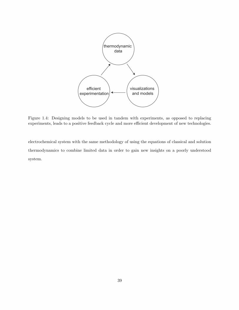
1.4 Designing models to be used in tandem with experiments, as opposed to replacing
experiments, leads to a positive feedback cycle and more efficient development of
new technologies. . . . . . . . . . . . . . . . . . . . . . . . . . . . . . . . . . . . . . . 39
2.1 Illustration of the thermodynamic system. . . . . . . . . . . . . . . . . . . . . . . . . 54
3.1 a) exchange of species A and B through a permeable membrane separating solutions
α and β. b) species A and B must undergo a redox reaction in order to exchange
between the metal and electrolyte . . . . . . . . . . . . . . . . . . . . . . . . . . . . . 61
3.2 Hypothetical placement of EA, EB, and ES on electrochemical potential series. In
this example, Eref = 0. . . . . . . . . . . . . . . . . . . . . . . . . . . . . . . . . . . 64
3.3 Equilibrium electrochemical synthesis diagram for arbitrary binary A-B, where A is
the more noble element on the electrochemical potential series, and A and B form a
completely miscible metallic solution. . . . . . . . . . . . . . . . . . . . . . . . . . . . 67
3.4 Equilibrium electrochemical synthesis diagram for the Pr−Nd/Pr2O3−Nd2O3 sys-
tem at 1323K. At this temperature, Pr and Nd form a completely miscible liquid. . . 68
15

3.5 Equilibrium electrochemical synthesis diagram for the Ag−Ni/AgCl2−NiCl2 system
at 1773K. At this temperature, Ag and Ni phase separate to form two different liquid
solutions. . . . . . . . . . . . . . . . . . . . . . . . . . . . . . . . . . . . . . . . . . . 69
3.6 Comparison of Raoultian, Henrian, and Wagner-Allanore reference states. Henrian
activities are scaled according to the value of γ∞, while Wagner-Allanore activities
are scaled according to the activity coefficient of A, γA, which may not be constant
with concentration, unlike the Henrian case. The composition coordinate of the
Wagner-Allanore reference state is also rescaled along the A−B pseudobinary. . . . 74
4.1 Phase diagram of the Ni-Co system. At 823K, Ni and Co form a fully miscible FCC
solid solution. . . . . . . . . . . . . . . . . . . . . . . . . . . . . . . . . . . . . . . . . 78
4.2 a) Electrochemical synthesis diagram for Ni − Co/NiCl2 − CoCl2 system at 823K
where xNiCl2 = xCoCl2 = 2wt%. b) Wagner-Allanore activity coefficient ρ for
CoCl2. : Values calculated for: ENi − ECo = 0.2V (from ideal solution), and
ENi − ECo = 0.185V (from cyclic voltammetry peaks). ;: experimental concentra-
tion of Co in Ni cathode after chronopoteniometry at 50mA/cm2, 200mA/cm2, and
500mA/cm2 [Choi2020]. . . . . . . . . . . . . . . . . . . . . . . . . . . . . . . . . . 81
4.3 Wagner-Allanore activity coefficient ρCoCl2 calculated from experimental concentra-
tion of Co in Ni cathode after electrolysis at 50mA/cm2, 200mA/cm2, and 500mA/cm2,
whenxCoCl2
xNiCl2+xCoCl2
= 0.2 (W) , 0.33 (5), and 0.5 (;) [Choi2020]. . . . . . . . . . . . 82
4.4 Comparison of electrolyte composition and cathode concentration after electrolysis
at 50mA/cm2, 200mA/cm2, and 500mA/cm2, whenxCoCl2
xNiCl2+xCoCl2
= 0.2 (W) , 0.33
(5), and 0.5 (;) [Choi2020]. . . . . . . . . . . . . . . . . . . . . . . . . . . . . . . . 83
4.5 Comparison of ρCoCl2 calculated from experimental concentration of Co in Ni cathode
after electrolysis at 50mA/cm2, to ideal solution assumption forxCoCl2
xNiCl2+xCoCl2
= 0.2
(W) , 0.33 (5), and 0.5 (;). Ideal solution model: [Choi2020]. . . . . . . . . . . . 84
16

4.6 Electrochemical synthesis diagram for for the Pr − Nd/Pr2O3 − Nd2O3 system at
1323K with: : predicted concentration of Nd in Pr based on ENi − ECo = −5mV ,
;: calculated from experimental results [Milicevic2017]. . . . . . . . . . . . . . . . 87
5.1 Standard-state electrochemical series for sulfides at 1523K, plotted v. Cu/Cu2S
reference [Bale2016, Barton1980]. . . . . . . . . . . . . . . . . . . . . . . . . . . . 95
5.2 Electrochemical synthesis diagram for for the Ag−Cu/Ag2S−Cu2S system at 1523K
with: : predicted concentration of Cu in Ag based on EAg − ECu = 257mV. . . . . 96
5.3 a) graphite crucible and cap used for sulfide melts and equilibration experiments b)
sulfide sample and metal taken from crucible post-equilibration experiment. . . . . . 99
5.4 Left) furnace setup used for sulfide melts and equilibrium experiments. Right)
schematic of setup showing hot zone and quench zone. . . . . . . . . . . . . . . . . . 100
5.5 Measured Cu content in Ag metal after equilibration with molten BaS-La2S3-Cu2S-
Ag2S at 1523K for 24 hours. . . . . . . . . . . . . . . . . . . . . . . . . . . . . . . . . 102
5.6 Calculated activity coefficient ρCu2S in BaS-La2S-Cu2S-Ag2S after equilibration with
Ag metal at 1523K for 24 hours. . . . . . . . . . . . . . . . . . . . . . . . . . . . . . 103
5.7 SEM image of typical microstructure of Ga-quenched BaS-La2S-Cu2S-Ag2S elec-
trolyte with an electroactive content of 40% Cu2S and 60% Ag2S. The “primary
phase” had an average Ag content of 65% relative to Cu, while the “secondary
phase” contained an average of 52%. No significant segregation trend was observed
in the tertiary phase. . . . . . . . . . . . . . . . . . . . . . . . . . . . . . . . . . . . 105
5.8 Measured overall Ag content relative to Cu in a BaS-La2S-Cu2S-Ag2S electrolyte
with an electroactive content of 40% Cu2S and 60% Ag2S, as a function of height
inside the crucible. . . . . . . . . . . . . . . . . . . . . . . . . . . . . . . . . . . . . . 106
5.9 Measured Ag content relative to Cu in the primary and secondary phases of a BaS-
La2S-Cu2S-Ag2S electrolyte with an electroactive content of 40% Cu2S and 60%
Ag2S, as a function of height inside the crucible. . . . . . . . . . . . . . . . . . . . . 107
17
6.1 Left) schematic of electrochemical cell used for Cu-Ag separation experiments. Right)
cathode and electrolyte after electrolysis experiment . . . . . . . . . . . . . . . . . . 118
6.2 Chronopotentiometry measurements in a BaS-La2S3-Cu2S-Ag2S electrolyte for cath-
odes containing varying starting amounts of Cu. Cathode current density: 12mA/cm2.
Temperature: 1523 K. . . . . . . . . . . . . . . . . . . . . . . . . . . . . . . . . . . . 120
6.3 Equilibrium electrochemical synthesis diagram showing change in cathode composi-
tion before and after electrolysis for a BaS-La2S3-Cu2S-Ag2S electrolyte containing
equimolar proportions of Cu2S and Ag2S. : equilibrium Cu content in Ag cathode
for this electrolyte. . . . . . . . . . . . . . . . . . . . . . . . . . . . . . . . . . . . . . 121
6.4 Fe-Cu phase diagram. . . . . . . . . . . . . . . . . . . . . . . . . . . . . . . . . . . . 124
6.5 a) Fe-Cu-C phase diagram when xCxF e+xC
= 0.17. b) equilibrium electrochemical syn-
thesis diagram for the Fe−Cu−C/FeS−Cu2S system at 1573K. At this temperature,
cast iron and Cu phase separate to form two different liquid solutions and solid C. :
predicted Cu content in cast iron (2 mol%), assuming ideal behavior in the electrolyte.125
6.6 Equilibrium electrochemical synthesis diagram for the Fe−Cu−C/FeS−Cu2S system
at 1573K for a cast iron cathode containing 19mol%C showing measured equilibrium
Cu content in cathode () as well as the cathode composition ranges after various
electrolysis experiments. . . . . . . . . . . . . . . . . . . . . . . . . . . . . . . . . . . 127
7.1 Schematic of a typical Fe-R-B magnet microstructure showing the magnetic 2-14
grains separated by a rare earth rich “other metallic phase” at the grain boundaries. 135
7.2 Overview of main processing steps in Fe-R-B magnet production. Highly oxidized
waste such as magnet sludge is produced mainly during the jet milling and machining
steps. . . . . . . . . . . . . . . . . . . . . . . . . . . . . . . . . . . . . . . . . . . . . 136
7.3 Overview of the current magnet sludge recycling process. Commercial magnet sludge
recycling occurs at the primary rare earth smelter. . . . . . . . . . . . . . . . . . . . 138
7.4 Comparison between actual magnet manufacturing (left) and the modeling steps
used herein (right). . . . . . . . . . . . . . . . . . . . . . . . . . . . . . . . . . . . . . 144
18
7.5 Calculated phase distribution in the simulated magnet after melting and casting with
no additional oxygen added (baseline case). . . . . . . . . . . . . . . . . . . . . . . . 146
7.6 Modeled distribution of rare earth elements among phases in baseline case. Rare
earth containing phases present: Dy: 100% Fe14Dy2B, Ce: 100% Ce2C3, Nd: 2%
Nd2O3, 96% Fe14Nd2B, 2% Nd2B5 Pr: 82% Pr and 18% PrAl2, La: 100% LaC2,
Gd: 14% Gd2O3, 86% GdS. . . . . . . . . . . . . . . . . . . . . . . . . . . . . . . . . 146
7.7 Calculated changes in phases present as oxygen content is increased from 0.09wt% to
5.4wt%. l: 2-14 phase, s: “other metallic” grain boundary phase, n: oxide phase.
After the grain boundary phase is completely oxidized near 1.8wt%, the 2-14 phase
begins to break down into oxide and more metallic phases. . . . . . . . . . . . . . . . 147
7.8 Modeled distribution of rare earth elements among phases with 5.4wt% O present.
Rare earth containing phases present: Dy: 100% Dy3Al5O12 Ce: 15% CeO2 85%
CeCrO3 Nd: 2% Nd3Al5O12, 45% NdBO3, 18% Fe14Nd2B, 35% Fe8Nd Pr: 100%
Fe8Pr Gd: 100% Gd3Al5O12 . . . . . . . . . . . . . . . . . . . . . . . . . . . . . . . 148
7.9 a) minimum Gibbs energy (∆G) needed to reduce equilibrated magnet sludge. b)
minimum Gibbs energy (∆G) to reduce magnet sludge with addition of the enthalpy
(∆H) to heat the material to temperature. —: modeled case where RE oxides are
separated prior to treatment. - - -: modeled case where sludge is reduced as a whole. 152
7.10 Calculated changes in phases present as O content in magnet sludge is reduced from
5.4% to 0% at 1773K. s: rare earth rich metallic phase (no Fe), n: oxide phase ,
l: metallic phases containing Fe and rare earth, u: Fe-rich metallic phase (no rare
earth). As oxygen is removed, Fe and rare earths interact to create new phases. . . . 153
7.11 Steps for direct recycling of magnet sludge. . . . . . . . . . . . . . . . . . . . . . . . 156
7.12 Ellingham diagram showing the ∆G of formation of relevant rare earth oxides and
calcium oxide, a popular choice for reductant in rare earth recycling. ∆Gf is very
similar for the various rare earths, highlighting their chemical similarity and the
resulting difficulty in purification from ore. . . . . . . . . . . . . . . . . . . . . . . . 158
19

A.1 Plot showing the relationship between the concentration of B in the cathode and
BX in the electrolyte, as well as the calculated distribution for each concentration.
Both metal and electrolyte are assumed to follow the regular solution model, with
T=1250K, Zmetal=10, Zelectrolyte=10, Ωmetal=300, Ωelectrolyte=-300. . . . . . . . . . . 180
A.2 a) ∆Gmix for sample metallic and electrolyte systems. b) Sum of ∆Gmixmetal and
∆Gmixelectrolyte. . . . . . . . . . . . . . . . . . . . . . . . . . . . . . . . . . . . . . . . . 182
A.3 Distribution of La and Nd between a LiCl-KCl electrolyte and a Cd cathode. s:
: modeled distribution from thermodynamic data and summed Gibbs energies of
mixing La-Nd and LaCl3-NdCl3. : experimentally determined distribution. Data
from [Ackerman1991, Ackerman1993]. . . . . . . . . . . . . . . . . . . . . . . . . 183
B.1 SEM image of quenched sulfide from Ag solubility experiments in BaS-Cu2S elec-
trolyte. Primary phase composition (mol%): 37% S, 29% Ba, 29% Cu, 5% Ag.
Secondary phase composition (mol%): 39 % S, 59% Ba, 2% Cu. . . . . . . . . . . . 192
B.2 SEM image of quenched sulfide from Au solubility experiments in BaS-Cu2S elec-
trolyte. Primary phase composition (mol%): 34% S, 32% Ba, 33% Cu. Secondary
phase composition (mol%): 37% S, 60% Ba, 2% Cu. Tertiary phase composition
(mol %): 33% S, 29% Ba, 17% Cu, 21% Au . . . . . . . . . . . . . . . . . . . . . . . 193
B.3 a) BaS-La2S-Cu2S ternary concentrations tested during isothermal experiment. b)
custom-designed graphite crucible showing sample wells and drill holes. c) example
of typical “melted”, “unmelted”, and “somewhat melted” samples post-experiment. . 195
B.4 Estimated isothermal projection of BaS-La2S-Cu2S system at 1473 K based on ob-
served melting behavior. . . . . . . . . . . . . . . . . . . . . . . . . . . . . . . . . . . 197
20

List of Tables
5.1 Cu content in Ag after equilibration and measured ρCu2S . . . . . . . . . . . . . . . 104
6.1 Cu content in cathode measured before and after electrolysis at 12mA/cm2. . . . . 120
7.1 Modeled Gibbs energy of 2-14 compounds modified to limit reaction with oxygen.
Real stoichiometry: Fe(14.00018), R(1.99988), B(0.9994) . . . . . . . . . . . . . . . 141
7.2 Elemental compositions used for calculations with no additional oxygen. Initial:
compositions estimated from published reports. Post-V IM : calculated after “ini-
tial” composition was equilibrated at 1723K to simulate treatment in vacuum induc-
tion melting furnace. . . . . . . . . . . . . . . . . . . . . . . . . . . . . . . . . . . . . 143
7.3 Comparison of theoretical energy needed for the existing magnet sludge recycling
method and the alternative of direct reduction of entire sludge without primary feed
or elemental separation. . . . . . . . . . . . . . . . . . . . . . . . . . . . . . . . . . . 157
21

22

Chapter 1
Introduction
Development of new, sustainable methods to process metals are desperately needed by modern
society, which must reconcile the benefits of technology and industrialization with the social and
environmental costs of such development. Metals production carries the highest environmental
footprint of all materials production in terms of greenhouse gas emissions (CO2-equivalent) [1], an
impact that is only posed to climb. Recent trends predict the amount of metals in-use globally will
increase 5 to 10 times current amounts by 2050 [2].
Furthermore, the scale-up of sustainability in other industries, such as the energy sector, is
inherently coupled to the metals industry, which itself is a web of interconnected elements that are
mined or processed together. For example, wind power relies on dysprosium-containing magnets,
which must be mined and partially processed alongside other rare earths [3, 4]. The key elements
in a photovoltaic solar cell, such as indium, germanium, and tellurium, are linked to the production
of base industrial metals copper and zinc, as well as toxic arsenic and cadmium [5]. In absence of
an effort to reduce the environmental impact of metals processing, the greenhouse gasses emitted
during metal production may in fact offset the benefits of the green technologies that require
them. [6].
Electrochemical reduction of metal ores is a pathway to greener extraction [7], with the ability
to significantly reduce emissions associated with metal production. By utilizing the electron to
decompose an oxidized species, according to the reaction:
23
AX → A+X (1.1)
where
An+ + ne− → A
Xn− → X + ne− (1.2)
only electricity is necessary, meaning that the footprint of this process is tied primarily to the
method of electricity generation [8]. If renewable energy sources are used to drive electrolysis, then
the emissions of greenhouse gasses such as CO2 and SO2 from metal production can be dramatically
reduced, or even eliminated.
At the cornerstone of electrochemical metal processing, or electrometallurgy, is the electrolyte,
the media which hosts the ions that are either oxidized or reduced inside the cell. Aqueous elec-
trolytes are popular for their low-temperatures and well-established chemistries, and are the system
of choice for electrowinning or electrorefining many metals such as zinc, nickel, copper, silver, and
gold. However, low-temperature aqueous systems are often plagued by slow kinetics, which in turn
lead to the necessity of operating at high current densities. When the electrodes are solid, as in
room temperature processes, then operating this way can cause dendritic growth. These dendrites
can break off and fall to the bottom of the cell with anode slimes, a collection of species insoluble
in the electrolyte.
Slimes pose an additional challenge to metal processing sustainability. Electrolysis must be
periodically stopped, so the cell can be cleaned and the slimes collected. In the case of copper
electrorefining, these slimes can contain valuable precious metals (10.5 wt% Ag and 1.8 wt% Au
were found in slimes at Sumitomo Metal Mining Co. Ltd. [9]), and some slimes can contain up to
50wt% Cu due to dendrite break-off [10], highlighting the inefficiency of this process.
Higher temperature, non-aqueous electrolytes operating with liquid cathodes do not produce
slimes. The most industrially important electrometallurgical technology utilizing a high tempera-
ture electrolyte and a liquid cathode is aluminum production via the Hall-Heroult process [11], but
24

the method is used for many reactive metals, including the rare earths [12].
Recently, new electrochemical technologies are pushing the boundaries of processing conven-
tions. Novel high temperature electrolytes such as molten sulfides [13, 14] and oxides [15] generally
have greater solubility for a wider range of elements than their aqueous counterparts, and are being
investigated to develop new extraction methods for base metals such as copper and iron. The bene-
fits of using a high temperature electrolyte and liquid electrode has even led to their implementation
in new battery designs, the liquid metal battery [16].
With new technologies come new challenges, and in the case of high temperature electrolytes,
enhanced solubility is both a benefit and a detriment. When multiple species are soluble in an
electrolyte, they can compete with each other for dominance of the cell’s redox reaction. Even
if the electrolyte is well-understood, the link between electrolyte properties and the composition
of the reduced metal at the cathode is unclear, and the relationship is difficult to quantify, with
efforts so far focusing on cathode chemistry and leaving the electrolyte generalized [17]. Novel
electrolytes are even more challenging. In these cases, the composition of the final metal product
cannot be guaranteed a priori, and many experiments are required to effectively develop the new
technology. In order to move forward with newer and greener electrochemical processes, then, the
study of selectivity in high temperature electrolysis is necessary.
1.1 Background on Selectivity in Electrochemistry
Except in notable cases, such as praseodymium-neodymium production from a mixed oxide [12],
the desired electrolyzed product tends to be a nearly pure metal. Purification tends to be achieved
through either pre-processing to ensure a pure electrolysis feedstock, as in the Bayer process for
aluminum production [18], or by carefully selecting a supporting electrolyte insoluble to unwanted
species, such as silver and gold in copper anode electrorefining [19]. Therefore, if these new elec-
trometallurgical routes are to be competitive with existing technology, they must be selective to
the metal of interest.
However, pre- and post- processing to avoid selectivity issues are not always practical. When
25

trying to recover metals from nuclear waste, a series of processing steps will introduce more points
of possible radioactive contamination, and separation in one unified electrochemical cell is prefer-
able [20, 21]. Additionally, significant energy expenditures and waste production result from pu-
rification steps, making these routes unattractive to recycling technologies that seek to break away
from the “back-to-the-smelter” approach currently used for many metals [4, 22–24].
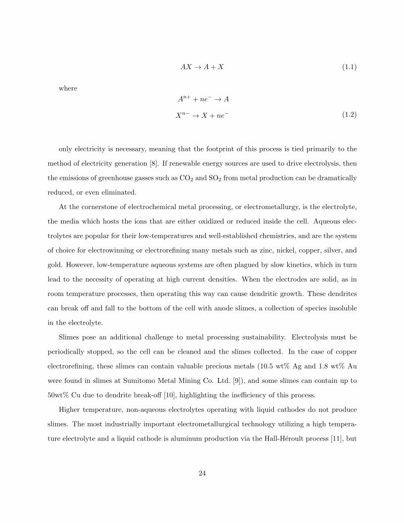
There is a rich body of literature on electrochemical selectivity from research on nuclear waste
processing. In 1989, the problem was addressed in a patent detailing an electrorefining cell for
separating uranium from plutonium in a molten chloride electrolyte [20]. Figure 1.1 shows the
schematic of the cell proposed in the patent. This cell featured a system of raising and lowering
cathode baskets. When a significant change in voltage was detected, indicating that plutonium
was now being deposited alongside uranium, the “pure” uranium cathode basket was raised and
an “alloy” cathode basket was lowered.
In addition to a new cell design, selectivity research in nuclear waste treatment also attempted to
probe the relationship between the electrode alloys, the electrolyte composition, and the dominating
redox reaction in hopes of enhancing the efficiency of electrorefining. Equilibration experiments
were carried out to study the partitioning of elements between a metal electrode and chloride
electrolyte [25–28]. This led to the development of “distribution” or “separation factor” as a means
of quantifying the selectivity of two elements. It is given by the ratio of two elements in the metal
electrode over the ratio of those same elements in the electrolyte after equilibrium. For elements A
and B present in the electrolyte as AX and BX such that there are two competing decomposition
reactions:
AX → A+X
BX → B +X (1.3)
Distribution can be given by:
26

Figure 1.1: Schematic of a molten salt electrorefining cell for selective refining of uranium, from [20].
27

D =
xAxBxAXxBX (1.4)
Further discussion of the utility of a distribution-based approach to modeling electrochemical
selectivity will be given in Appendix A.
Other endeavors to study the factors contributing to selectivity have focused on the chemistry of
the electrolyte and the role of the supporting electrolyte. In their investigation of electrochemically
separating Mg and Mn from Al cans for recycling, Antony Cox and Derek Fray examined how
electrolyte composition affected the electrode potential of each element, and its effect on the chloride
series [29]. By only varying the concentration of the NaCl-MgCl2 supporting electrolyte by about
20wt%, the electrode potentials of Mg, Mn, and Al were observed to change by as much as 50mV.
This phenomena may be explained by changes in the activities of AlCl3, MnCl2, and MgCl2.
Although only the concentration of MgCl2 and NaCl were changed, this resulted in an overall
change in the thermodynamic properties of the entire Al-Mg-Mn-Na-Cl quinternary system. This,
in turn, changed the activities of AlCl3 and MnCl2, even if their concentration remained the same.
Consider the equation for reduction of a generic metal chloride MexCly:
2
yMexCly →
2x
yMe + Cl2 (1.5)
The Gibbs energy of this reaction can be broken down into the standard state reaction, ∆G,
and the effect solution behavior will have on this reaction, measured by activity as well as fugacity
(or partial pressure assuming chlorine behaves as an ideal gas):
∆Gr = ∆G +RT lnacMepCl2abMexCly
(1.6)
Neglecting for the moment the effects of the gas (pCl2), if aMe > aMexCl2 , then the metallic
Me carries a higher energy of mixing in the metal phase than MexCly in the electrolyte. This will
raise the overall Gibbs energy of reaction. Conversely, if aMe < aMexCl2 , then MexCly carries a
28
higher energy of mixing, which will lower the Gibbs energy of reaction. The activity of MexCly
can be affected by a variety of factors, including temperature and pressure as well as the overall
electrolyte composition. Thus, even if the concentration of MexCly itself does not change, changing
the concentrations of other species will change those species’ activity, and in turn change the activity
of MexCly [30].
1.2 Methods to Determine Electrolyte Activity
Understanding the activities of electrolyte species is essential to understanding selectivity in
electrolysis. Because activity contributes to the Gibbs energy of the decomposition reaction, it will
influence which redox couple dominates during cell operation. Fortunately, the study of activity is
an established practice in thermodynamics, with a variety of methods presently in use to measure
and quantify it.
1.2.1 Experimental Methods
Equilibrium-Based Methods
In equilibrium activity measurements, the composition of a species in a known phase, or ref-
erence phase, is directly connected to its composition in an unknown phase by the equilibrium
constant for the chemical reaction of moving between phases. One common application of this
method are vapor-pressure studies.
Consider a molten salt electrolytic species AX. If the partial pressure of AX in the gaseous
phase above the liquid can be measured, than the activity of AX in the liquid electrolyte may be
determined by the equation:
alAX =pAXPAX
(1.7)
where PAX is the vapor pressure of pure gaseous AX. If AX cannot be assumed to be an ideal
gas, fugacity may be substituted into this relationship. This method is a popular and accurate
way to probe electrolyte activity, and has been extensively used to gather data on molten salt
29
electrolytes [31–33].
In theory, this principle can be extended to any system where two phases can be brought
into equilibrium with one another (i.e. liquid-solid or liquid-liquid, not only liquid-gas). The phase
under investigation is the “unknown phase”, in this case the liquid electrolyte, and the second phase
is the “reference phase”, with known properties that can be found in a database or reference text
such as [30, 34]. This method is useful when vapor pressure methods are not possible, for example,
if AX disassociates upon vaporization according to an unknown mechanism. Equilibrium methods
have been used to probe the properties of high-temperature liquids [35, 36], and are possible as
long as the equilibrium constant of the phase change reaction is known and thermochemical data
on the reference phase is available.
Electrochemical Methods
An alternative method of activity measurements is electrochemical potential difference mea-
surements (formerly electromotive force measurements). This method is attractive because the use
of a potentiostat to record potential differences allows for highly precise measurements, down to
the order of microvolts. Additionally, thermodynamic properties of high temperature systems may
be probed in-situ, unlike some equilibration measurements which must first be quenched before
evaluation.
The fundamental principle for this study is measurement of the potential difference between
electrodes. The system being probed must have a working electrode (WE) and at least one reference
electrode (RE). The difference between these two is given by:
∆Ecell = EWE − ERE
∆Ecell = −RTnF
lnaAaB
(1.8)
where the activity aB is known through the use of a stable and well-defined reference electrode.
This method has been used to probe systems that could be used for new innovative electro-
chemical technologies (see [37–39] for a series of studies used in development of the liquid metal
battery), as well as to inform on molten salt electrolytes (see [31, 40, 41]).
30

One drawback of potential difference measurements is their dependency on a reference electrode
at which a consistent and known reaction occurs. Such an electrode must be resistant to contamina-
tion by other elements that could drift or change its potential. The reactive nature of most molten
salt electrolytes makes this endeavor challenging. It is possible to inhibit transfer of problematic
species through use of a selective solid electrolyte membrane such as β”-Al2O3 (see [42] and the
references within), but the success of this method is dependent on the accuracy of the assumption
that the molten salt does not interact with membrane.
Recently, a novel method of electrochemical activity measurements using alternating current
cyclic voltammetry (ACV) has been proposed [43]. This is an attractive alternative. The enhanced
accuracy of ACV as well as its ability to segregate different electrochemical phenomena to different
Fourier harmonics, allowing for a more thorough evaluation, has been demonstrated [44–49].
1.2.2 Computational Methods
With the increase in modern computational power has come expanded interest in computational
efforts to determine thermodynamic properties. Broadly speaking, these efforts can be divided into
two categories: ab-initio, or “first principles” calculations, and CALPHAD modeling. Ab-initio
techniques attempt to solve the equations of quantum and statistical mechanics in order to define all
materials properties (see [50] for more information). However, the ability to solve these relationships
at higher temperature, when entropic contributions start to play a key role, is limited. Therefore
this discussion will focus instead on CALPHAD modeling, which is more common in studying the
thermochemistry of high temperature liquids.
CALPHAD is an acronym for “Calculation of PHAse Diagrams”, and it is an interpolation-
extrapolation method. Expressions for the Gibbs energy of pure substances are calculated first,
linearly expanded in terms of T. Such data can be calculated by fitting experimental data, by
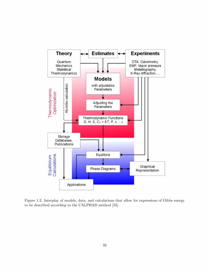
comparison to similar systems, or from ab-initio techniques. Figure 1.2 shows the interplay of
various data sources in building CALPHAD models. Scientific Group Thermodata Europe [51]
produced one of the most comprehensive publicly available databases for pure elements, as well as
references for the data used to make their functions. This database forms the core of the models
31

for the two main CALPHAD softwares available today, FactSage [52] and Thermo-Calc [53].
In the CALPHAD method, pure substance data are used as end members for a binary expression,
which is determined by the software in the same matter as pure substances (fitting, comparison,
and calculation). Information on a system binary is fit to a statistical solution model that can
also be linearly expanded in terms of T. As the ultimate goal is convergence, the fitting models
are not general to the thermodynamics of every system. Instead, they must be carefully selected
by the modeler based on their assumptions. For example, solid solutions at low temperature
and off-stoichiometry compounds are commonly modeled using the Compound Energy Formalism
(CEF) [54]:
G = XAG0A +XBG
0B +RT (XAlnXA +XBlnXB) +Gex
Gex = XAXB
∑n≥0
nL(A,B)(XB −XA)n(1.9)
The summation may be expanded as necessary until convergence is reached during interpolation.
Statistical expressions of liquids are far more challenging, and they are commonly modeled using
a random-mixing Bragg-Williams approximation [55]. Models have been derived attempting to
incorporate the nonrandom nature of liquid mixing, one example being the Modified Quasichemical
Model (MQM) [56–59], adapted from the Quasichemical Model [60]. The full MQM is given by:
G = (nA,V aG0A,V a + nB,V aG
0B,V a)− T∆Sconfig +
nAB,V a2
∆gAB,V a
∆gAB = ∆g0AB +
∑i≥1
gi0ABXiAA +
∑j≥1
g0jABX
jBB
(1.10)
where Sconfig is represented by 1-dimensional Ising Model [61]. ∆g contains information about
the coordination number Z as well, although this value is used as another fitting parameter and
may be changed by the modeler in order to optimize fit.
The many complex fitting parameters demanded by this model arises from its lack of an accurate
statistical description for entropy. In order to compensate for the use of the 1-D Ising Model, all
other parameters, including end-member data, must be optimized. Unfortunately, reliance on such
fitting techniques cause challenges in accuracy of obtaining new information by extrapolating the
32
Thermo-Calc SoftwareThe CALPHAD method
Figure 1.2: Interplay of models, data, and calculations that allow for expressions of Gibbs energyto be described according to the CALPHAD method [53].
33

CALPHAD-generated Gibbs energy expression into unstudied regions. Rinzler and Allanore showed
that by expanding the definition of entropy in the quasichemical model to include just one other
mode of entropy, in this case electronic entropy, the accuracy of liquid models increased [62].
Entropic contributions are significant in molten salts. These electrolytes are high temperature,
multicomponent liquids with complex ionic and electronic interactions. Such features make CAL-
PHAD modeling challenging: even if enough data are obtained to build a model for the system, the
divergence between entropy as described in the fitted equations and entropy in the actual liquid
solution will cause inaccurate extrapolation to new concentrations and conditions. Additionally,
the success of the CALPHAD method is predicated on the existence of accurate experimental data
for the system. If an electrolyte is novel, with unknown thermochemical properties, and also reac-
tive enough that traditional activity measurements are difficult, then it cannot be modeled using
CALPHAD techniques.
1.3 Molten Sulfides: A Unique Electrolyte for Both Primary and
Secondary Metal Processing
Molten sulfides are a class of electrolyte that sit at the intersection of novel, reactive, and
high-temperature: a challenging system to study thermodynamically. Furthermore, its exceptional
solubility properties for multiple elements force the electrochemist to face issues of selectivity head-
on. However, it is molten sulfide’s ability as a high temperature solvent that enable its use in new
electrochemical technologies.
1.3.1 Precious Metals and Molten Sulfide Electrolysis
Due to solubility limitations of aqueous media, extracting precious metals, whether from copper
ore or electronic waste, must be done sequentially. Typically, these metals are separated from each
other during electrorefining, where an aqueous electrolyte soluble specifically to the species of
interest is chosen. This method starts with the more reactive metal (such as Cu), and sequentially
moves on to refine more more noble metals (Ag, followed by Au, followed by PGM). When Cu is
34
refined, Ag, Au and PGM collect at the bottom of the cell in the slimes.
The anode slimes take primarily the form of selenides (containing the valuable metals), and
sulfates (containing base and special metals such as lead and arsenic, as well as some copper) [10, 63–
67]. There are many differing techniques for treating slimes, extensively discussed in literature [10,
68–70]. These methods often utilize a combination of pyro- and hydro- metallurgical techniques to
successfully extract metals, and are generally optimized for the typical slime composition at each
refinery. However, in all cases, this process can only be done in series, using multiple facilities and
separate streams for each metal. This is true regardless of the initial material’s status as a primary
ore or a secondary recycled waste.
Molten sulfides have already shown promise as a stable electrolyte with sufficient ionic conduc-
tivity to support electrolysis. They have been a successful media for electrolytic decomposition of
the sulfides of copper, molybdenum, and rhenium [14, 48]. Furthermore, copper, gold, silver, plat-
inum, and palladium have all been found in nature as sulfides [71–73], supporting the likelihood
that they could be solvated in a molten sulfide electrolyte. Preliminary tests of precious metal
solubility in molten sulfides will be discussed in Appendix B.
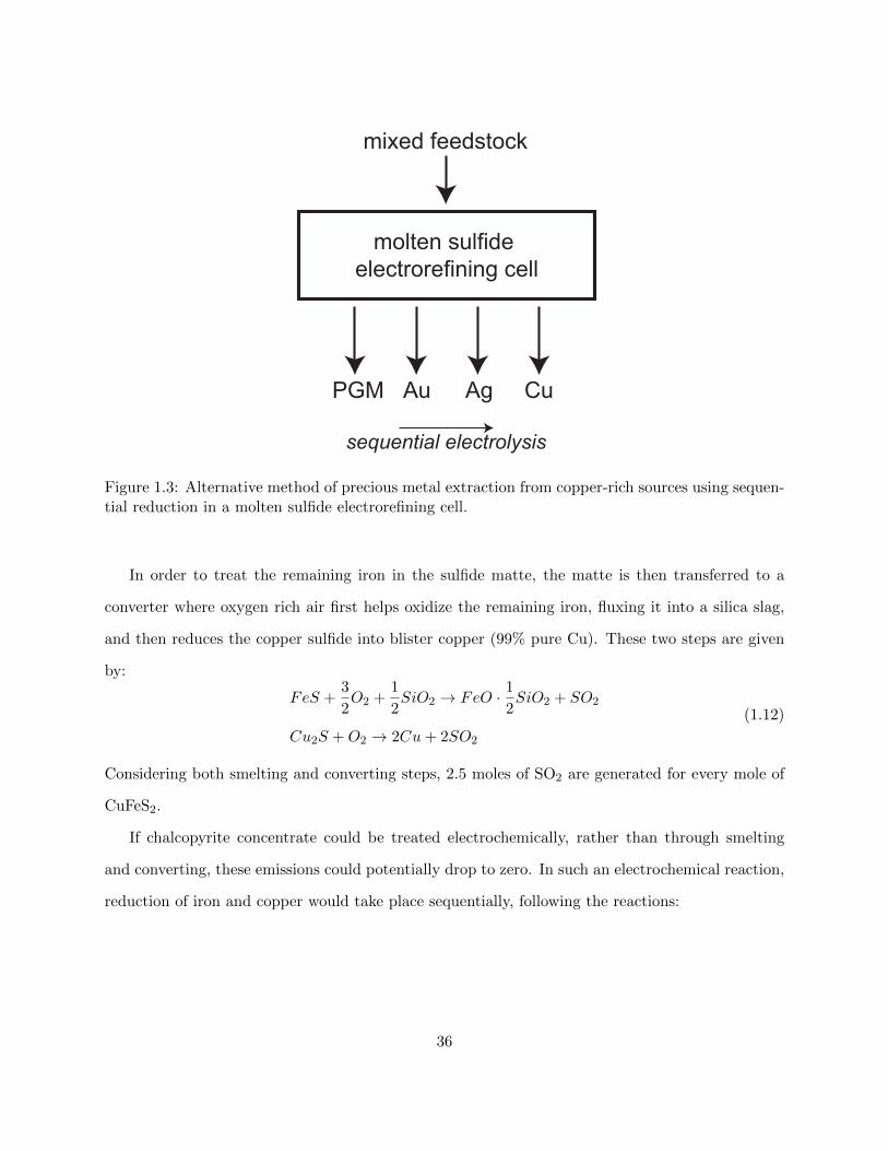
Figure 1.3 shows a possible alternative to treating and extracting precious metals from copper-
containing sources. Such a process would be enabled by the unique solvating behavior of molten
sulfides, and is inspired by the sequential refining cell proposed for nuclear waste treatment [20].
1.3.2 Copper Ore and Molten Sulfide Electrolysis
Chalcopyrite is one of the most commonly processed minerals in copper-bearing ores, with a
chemical composition of CuFeS2 [19]. Once the ore is concentrated to isolate this mineral, a product
with almost equimolar amounts of iron and copper remains.
The next step in copper processing is matte smelting in order to segregate iron to an oxide
(slag) phase and copper to a sulfide (matte) phase. The chemical reaction is given below for one
mole of chalcopyrite as:
CuFeS2 +13
8O2 →
1
2(Cu2S ·
1
2FeS) +
3
4FeO +
5
4SO2 (1.11)
35
molten sulfide electrorefining cell
Au Ag CuPGM
mixed feedstock
sequential electrolysis
Figure 1.3: Alternative method of precious metal extraction from copper-rich sources using sequen-tial reduction in a molten sulfide electrorefining cell.
In order to treat the remaining iron in the sulfide matte, the matte is then transferred to a
converter where oxygen rich air first helps oxidize the remaining iron, fluxing it into a silica slag,
and then reduces the copper sulfide into blister copper (99% pure Cu). These two steps are given
by:
FeS +3
2O2 +
1
2SiO2 → FeO · 1
2SiO2 + SO2
Cu2S +O2 → 2Cu+ 2SO2
(1.12)
Considering both smelting and converting steps, 2.5 moles of SO2 are generated for every mole of
CuFeS2.
If chalcopyrite concentrate could be treated electrochemically, rather than through smelting
and converting, these emissions could potentially drop to zero. In such an electrochemical reaction,
reduction of iron and copper would take place sequentially, following the reactions:
36

CuFeS2 →1
2Cu2S + Fe+
3
4S2
1
2Cu2S → Cu+
1
4S2
(1.13)
with 1 mole of S2 generated for every mole of Cu produced. Sulfur is solid at room temperature,
indicating that it can be easily collected downstream.
Such a process would have a great environmental benefit, but being able to control the selectivity
of this process in order to compete with industry standards of less than 1% Fe in blister copper is
critical to its success [19]. Both Cu and Fe are soluble in molten sulfides, but their standard state
free energies of sulfide formation are sufficiently close to each other to make co-deposition during
electrolysis highly probable.
There is significant evidence suggesting that the behavior of Cu2S and FeS vary significantly
from standard state behavior, and that molten sulfides in general do not follow the ideal solution
model. It is not uncommon for sulfide systems to show liquid-liquid miscibility gaps [74, 75], owing
partially to changes in electronic structure and behavior [62]. Therefore, an assessment of the
thermodynamics of a molten sulfide electrolyte used for Cu and Fe extraction is necessary in order
to evaluate how feasible separation in this system may be.
1.4 The Argument for a New Approach to Thermodynamic Study
at High Temperature
The ability to quickly determine electrolyte suitability is necessary if electrochemical technolo-
gies are going to meet the demands for sustainable processing. With their improved solubility, faster
kinetics, and environmentally benign anode products if an inert anode is used, high temperature
electrochemistry offers significant improvement over existing extraction and treatment methods.
When a new electrochemical system is screened for possible use in a new technology, one of
the first items for consideration is the placement of the species of interest on the standard state
electrochemical series. The more noble species will be deposited on the cathode first, and if there is
sufficient (≈ 200mV ) difference between that species and the next one on the series, a pure product
37

can be expected [76]. This behavior is then confirmed or refuted through a series of thermodynamic
and electrochemical experiments targeted at understanding the cell behavior. It is not possible to
know if the technology will be successful a priori.
Modelers often approach thermodynamics with the goal of eliminating these experimental steps.
If everything about a system can be determined computationally, then laboratory tests become
redundant. Unfortunately, computational power sufficient to utilize ab-initio techniques in high-
entropy, high-temperature systems is not yet available, and the success of the CALPHAD method
is predicated on the existence of accurate data for the system of study, as well as statistical models
that capture solution behavior. While this makes CALPHAD modeling useful for well-established
technologies, such as steelmaking, its ability to evaluate a truly novel system is presently lacking.
The models that will be presented and discussed in this thesis follow an alternative approach.
Designed from the start to be run in tandem with experiments, they fall in between experimental
analysis techniques and predictive modeling methods. These models will be grounded in the rela-
tively simple equations of solution thermodynamics, meaning they can be easily solved and utilized
without significant computational power or softwares. The intended outcome of such an approach
is detailed in Figure 1.4: experiments are used to generate thermodynamic data, which are then
fed into equations of classical thermodynamics and analyzed with visualizations in order to gain
new insight on a system. These insights are then used to design future experiments. Unlike other
modeling approaches, the models put forth in this thesis require very few data to analyze a system.
As such, systems with scattered or incomplete datasets may be evaluated.
In Chapter 2, I will put forth the central hypothesis of this thesis, providing a framework to
predict selectivity in high temperature electrochemistry. The selectivity models derived in Chapter 3
are done so with this alternative approach to modeling in mind: they are intended from the start
to be an aid to the electrochemist when exploring new systems and technologies. In Chapter 4,
I will verify the accuracy of this model by comparing results to already studied systems, and in
Chapters 5 and 6, I will demonstrate the utility of this alternative approach by using it to study
a novel system: molten sulfide electrolysis for copper and precious metal extraction. Finally, I
will extend the philosophy of this modeling approach in Chapter 7, where I will analyze a non-
38
thermodynamic data
efficient experimentation
visualizations and models
Figure 1.4: Designing models to be used in tandem with experiments, as opposed to replacingexperiments, leads to a positive feedback cycle and more efficient development of new technologies.
electrochemical system with the same methodology of using the equations of classical and solution
thermodynamics to combine limited data in order to gain new insights on a poorly understood
system.
39
Bibliography
[1] Edgar G. Hertwich. “Increased carbon footprint of materials production driven by rise in
investments”. In: Nature Geoscience 14.3 (Mar. 2021), pp. 151–155. issn: 1752-0894. doi:
10.1038/s41561-021-00690-8. url: http://www.nature.com/articles/s41561-021-
00690-8.
[2] M.A. Reuter et al. UNEP (2013) Metal Recycling: Opportunities, Limits, and Infrastructure,
A Report of the Working Group on the Global Metal Flows to the Inter-national Resource
Panel. Tech. rep. UNEP, 2013.
[3] Ayman Elshkaki and T. E. Graedel. “Dysprosium, the balance problem, and wind power
technology”. In: Applied Energy 136 (Dec. 2014), pp. 548–559. issn: 03062619. doi: 10.
1016/j.apenergy.2014.09.064.
[4] Osamu Takeda and Toru H. Okabe. “Current Status on Resource and Recycling Technology
for Rare Earths”. In: Metallurgical and Materials Transactions E 1 (June 2014), pp. 160–
173. issn: 2196-2936. doi: https://doi.org/10.1007/s40553-014-0016-7. url: http:
//link.springer.com/10.1007/s40553-014-0016-7.
[5] Ayman Elshkaki and T. E. Graedel. “Solar cell metals and their hosts: A tale of oversupply
and undersupply”. In: Applied Energy 158 (Nov. 2015), pp. 167–177. issn: 03062619. doi:
10.1016/j.apenergy.2015.08.066.
[6] Takuma Watari, Keisuke Nansai, and Kenichi Nakajima. “Review of critical metal dynam-
ics to 2050 for 48 elements”. In: Resources, Conservation and Recycling 155 (Apr. 2020),
p. 104669. issn: 18790658. doi: 10.1016/j.resconrec.2019.104669.
40
[7] Antoine Allanore. “Features and Challenges of Molten Oxide Electrolytes for Metal Extrac-
tion Fundamentals of Metal Extraction: The Electrolytic Path”. In: Journal of The Electro-
chemical Society 162.1 (2015), pp. 13–22. doi: 10.1149/2.0451501jes.
[8] Donald R. Sadoway. “New opportunities for metals extraction and waste treatment by elec-
trochemical processing in molten salts”. In: Journal of Materials Research 10.03 (Mar. 1995),
pp. 487–492. issn: 0884-2914. doi: 10.1557/JMR.1995.0487. url: http://www.journals.
cambridge.org/abstract%7B%5C_%7DS0884291400077086.
[9] C Segawa and T Kusakabe. “Current Operations in SMM’s Slime Treatment”. In: TMS
Extraction and Processing Division. Anaheim, Ca, 1996. url: http://www.isasmelt.com/
EN/Publications/TechnicalPapersBBOC/SMM’s%20Slime%20Treatment.pdf.
[10] Ailiang Chen et al. “Recovery of Silver and Gold from Copper Anode Slimes”. In: JOM
Journal of the Minerals, Metals and Materials Society 67.2 (2015), pp. 493–502. doi: 10.
1007/s11837-014-1114-9.
[11] Nguyen Quang Minh. “Extraction of Metals by Molten Salt Electrolysis : Chemical Funda-
mentals”. In: 37.January (1985), pp. 28–33. url: http://link.springer.com/content/
pdf/10.1007/BF03257510.pdf.
[12] Ksenija Milicevic, Thomas Meyer, and Bernd Freidrich. “Influence of electrolyte composition
on molten salt electrolysis of didymium”. In: ERES2017: 2nd European Rare Earth Resources
Conference. Santorini, 2017. doi: 10.13140/RG.2.2.13137.33122.
[13] Samira Sokhanvaran et al. “Electrochemistry of Molten Sulfides: Copper Extraction from
BaS-Cu 2 S”. In: Journal of The Electrochemical Society 163.3 (2016), pp. D115–D120. issn:
0013-4651. doi: 10.1149/2.0821603jes.
[14] Sulata K. Sahu, Brian Chmielowiec, and Antoine Allanore. “Electrolytic Extraction of Cop-
per, Molybdenum and Rhenium from Molten Sulfide Electrolyte”. In: Electrochimica Acta
243 (2017), pp. 382–389. issn: 00134686. doi: 10.1016/j.electacta.2017.04.071.
41
[15] Antoine Allanore, Lan Yin, and Donald R. Sadoway. “A new anode material for oxygen
evolution in molten oxide electrolysis”. In: Nature 497 (May 2013), pp. 353–356. doi: 10.
1038/nature12134. url: http://www.nature.com/articles/nature12134.
[16] Hojong Kim et al. “Liquid Metal Batteries: Past, Present, and Future”. In: Chemical Reviews
113.3 (2013), pp. 2075–2099. doi: 10.1021/cr300205k. url: http://sadoway.mit.edu/
wordpress/wp-content/uploads/2011/10/Sadoway%7B%5C_%7DResume/145.pdf.
[17] G. Kaptay. “The conversion of phase diagrams of solid solution type into electrochemical
synthesis diagrams for binary metallic systems on inert cathodes”. In: Electrochimica Acta
60 (Jan. 2012), pp. 401–409. issn: 00134686. doi: 10.1016/j.electacta.2011.11.077.
[18] James Metson. “Production of Alumina”. In: Fundamentals of Aluminum Metallurgy. Ed. by
Roger Lumley. Cambridge: Woodhead, 2011. Chap. 2, pp. 23–48. isbn: 978-1-84569-654-2.
[19] W.G Davenport et al. Extractive Metallurgy of Copper. Fourth. Elsevier Science, 2002. isbn:
0-444-50206-8.
[20] John P. Ackerman and William E. Miller. Electrorefining process and apparatus for recovery
of uranium and a mixture of uranium and plutonium from spent fuels. Nov. 1989.
[21] Timothy Lichtenstein et al. “Electrochemical deposition of alkaline-earth elements (Sr and Ba)
from LiCl-KCl-SrCl 2 -BaCl 2 solution using a liquid bismuth electrode”. In: Electrochimica
Acta 281 (Aug. 2018), pp. 810–815. issn: 00134686. doi: 10.1016/j.electacta.2018.05.
097.
[22] Jirang Cui and Lifeng Zhang. “Metallurgical recovery of metals from electronic waste: A
review”. In: Journal of Hazardous Materials 158.2-3 (2008), pp. 228–256. issn: 03043894.
doi: 10.1016/j.jhazmat.2008.02.001.
[23] Umicore Process. http://pmr.umicore.com/en/about-us/process/. url: http://pmr.umicore.
com/en/about-us/process/ (visited on 01/15/2018).
[24] C J Newman, D N Collins, and A J Weddick. Recent operation and environmental con-
trol in the Kennecott Smelter. Tech. rep. Magna, UT: Kennecott Utah Copper Corporation,
42
1999, pp. 1–17. url: http://www.kennecott.com/library/media/kennecott%7B%5C_
%7Dsmelter.pdf.
[25] John P Ackerman. “Chemical Basis for Pyrochemical Reprocessing of Nuclear Fuel”. In: Ind.
Eng. Chem. Res. 30.1 (1991), pp. 141–5. url: https://pubs.acs.org/sharingguidelines.
[26] John P. Ackerman and Jack L. Settle. “Distribution of plutonium, americium, and several rare
earth fission product elements between liquid cadmium and LiCl-KCl eutectic”. In: Journal
of Alloys and Compounds 199 (Sept. 1993), pp. 77–84. issn: 09258388. doi: 10.1016/0925-
8388(93)90430-U.
[27] M Kurata et al. “Distribution behavior of uranium, neptunium, rare-earth elements (Y, La,
Ce, Nd, Sm, Eu, Gd) and alkaline-earth metals (Sr,Ba) between molten LiC1-KC1 eutectic
salt and liquid cadmium or bismuth”. In: Journal of Nuclear Materials 227 (1995), pp. 110–
121.
[28] Y Sakamura et al. “Distribution behavior of plutonium and americium in LiCl–KCl eutec-
tic/liquid cadmium systems”. In: Journal of Alloys and Compounds 321 (May 2001), pp. 76–
83. issn: 09258388. doi: 10.1016/S0925-8388(01)00973-2.
[29] Antony Cox and Derek Fray. “Separation of Mg and Mn from Beverage Can Scrap using a
Recessed-Channel Cell”. In: Journal of The Electrochemical Society 150.12 (2003), pp. D200–
8. doi: 10.1149/1.1623768.
[30] C H P Lupis. Chemical Thermodynamics of Materials. New York: North-Holland, 1983. isbn:
9780444007797.
[31] Milton Blander. Molten Salt Chemistry. New York: Interscience Publishers, 1964, p. 775.
[32] O.J. Kleppa. “Thermodynamics of Molten Salt Mixtures”. In: Molten Salt Chemistry. Ed. by
G Mamantov and R. Marassi. Dordrecht: Springer, 1987, pp. 79–122. doi: 10.1007/978-94-
009-3863-2_4.
[33] T Forland. “Thermodynamic Properties of Fused Salt Systems”. In: Fused Salts. Ed. by B
Sunderheim. New York: McGraw-Hill, 1964, pp. 63–164.
43
[34] E.T. Turkdogan. Physical Chemistry of High Temperature Technology. New York: Academic
Press, 1980. isbn: 0-12-704650-X.
[35] Yun Lei et al. “Thermodynamic properties of the MnS-CuS0.5 binary system”. In: ISIJ
International 52 (2012), pp. 1206–1210. doi: 10.2355/isijinternational.52.1206. url:
https://www.jstage.jst.go.jp/article/isijinternational/52/7/52%7B%5C_
%7D1206/%7B%5C_%7Dpdf.
[36] Yun Lei et al. “Thermodynamic properties of the FeS-MnS-CuS0.5 ternary system at 1473 K”.
In: ISIJ International 53 (2013), pp. 966–972. doi: 10.2355/isijinternational.53.966.
url: https://www.jstage.jst.go.jp/article/isijinternational/53/6/53%7B%5C_
%7D966/%7B%5C_%7Dpdf.
[37] Hojong Kim et al. “Thermodynamic properties of calcium – magnesium alloys determined by
emf measurements”. In: Electrochimica Acta 60 (2012), pp. 154–162. issn: 0013-4686. doi:
10.1016/j.electacta.2011.11.023. url: http://dx.doi.org/10.1016/j.electacta.
2011.11.023.
[38] Jocelyn Marie Newhouse. “Modeling the operating voltage of liquid metal battery cells”.
PhD thesis. Massachusetts Institute of Technology, 2014. url: https://dspace.mit.edu/
handle/1721.1/89840.
[39] Sophie Poizeau et al. “Determination and modeling of the thermodynamic properties of liquid
calcium–antimony alloys ”. In: Electrochimica Acta 76 (2012), pp. 8–15.
[40] George J. Janz. Molten Salts Handbook. New York: Academic Press, Inc., 1967, p. 588.
[41] Y. K. Delimarskii and B. F. Markov. Electrochemistry of Fused Salts (Translated). Ed. by
Reuben E. Wood. Washington D.C.: The Sigma Press, Publishers, 1961, p. 338.
[42] Caspar Stinn and Antoine Allanore. “Thermodynamic and Structural Study of the Copper-
Aluminum System by the Electrochemical Method Using a Copper-Selective Beta” Alumina
Membrane”. In: Metallurgical and Materials Transactions B 49.6 (2018), pp. 3367–3380. issn:
1073-5615. doi: 10.1007/s11663-018-1400-y. url: http://link.springer.com/10.1007/
s11663-018-1400-y.
44

[43] Andrew H. Caldwell. “Alternating Current Voltammetry of High Temperature Electrolysis
Reactions”. Doctoral. Massachusetts Institute of Technology, 2020.
[44] Donald E. Smith. “AC polarography and related techniques”. In: Electroanalytical Chemistry:
A Series of Advances (I). Ed. by A J Bard. New York: Marcel Dekker, Inc., 1966. Chap. 1,
pp. 1–155.
[45] Anna A. Sher et al. “Appendix: Resistance Capacitance and Electrode Effects in Fourier
Transformed Large Amplitude Sinusoidal Voltammetry: The Emergence of Powerfl and In-
tuitively Obvious Tools for Recognition of Patterns of Behaviour”. In: Analytical Chemistry
76.21 (2004), p. 13. issn: 0717-6163.
[46] A. M. Bond et al. “Changing the Look of Voltammetry”. In: Analytical Chemistry 77 (2005),
186A–195A.
[47] Mary-Elizabeth Wagner et al. “Copper Electrodeposition Kinetics Measured by Alternating
Current Voltammetry and the Role of Ferrous Species”. In: Journal of The Electrochemical
Society 163.2 (2016), pp. D17–D23. issn: 0013-4651. doi: 10.1149/2.0121602jes. url:
http://jes.ecsdl.org/lookup/doi/10.1149/2.0121602jes.
[48] Samira Sokhanvaran et al. “Electrochemistry of Molten Sulfides: Copper Extraction from
BaS-Cu 2 S”. In: Journal of The Electrochemical Society 163.3 (2016), pp. D115–D120. issn:
0013-4651. doi: 10.1149/2.0821603jes.
[49] Bradley R. Nakanishi and Antoine Allanore. “Electrochemical study of a pendant molten
alumina droplet and its application for thermodynamic property measurements of Al-Ir”. In:
Journal of The Electrochemical Society 164.13 (2017), E460. doi: 10.1149/2.1091713jes.
[50] Materials Project. url: https://www.materialsproject.org/ (visited on 03/31/2021).
[51] A T Dinsdale. “SGTE data for pure elements”. In: CALPHAD: Comput. Coupling Phase
Diagrams Thermochem. 15.4 (1991), pp. 317–425.
45

[52] C. W. Bale et al. “FactSage thermochemical software and databases, 2010-2016”. In: Calphad
54 (Sept. 2016), pp. 35–53. issn: 03645916. doi: https://doi.org/10.1016/j.calphad.
2016.05.002.
[53] J.O. Andersson et al. “Thermo-Calc and DICTRA, Computational tools for materials sci-
ence”. In: Calphad 26 (2002), pp. 273–312.
[54] Mats Hillert. “The compound energy formalism”. In: Journal of Alloys and Compounds 320.2
(2001), pp. 161–176. doi: 10.1016/S0925-8388(00)01481-X. url: http://linkinghub.
elsevier.com/retrieve/pii/S092583880001481X.
[55] Terrell L. Hill. An Introduction to Statistical Thermodynamics. New York: Dover Publications,
Inc., 1986. isbn: 0-486-65242-4.
[56] A D Pelton et al. “The Modified Quasichemical Model I — Binary Solutions”. In: Metallurgical
and Materials Transactions B 31B.August (2000), pp. 651–659.
[57] Arthur D. Pelton. “A General ”Geometric” Thermodynamic Model for Multicomponent So-
lutions”. In: Calphad 25.2 (2001), pp. 319–328.
[58] Patrice Chartrand and Arthur D. Pelton. “The modified quasi-chemical model: Part III. Two
sublattices”. In: Metallurgical and Materials Transactions A 32.6 (2001), pp. 1397–1407. issn:
1073-5623. doi: 10.1007/s11661-001-0229-0.
[59] Arthur D. Pelton, Patrice Chartrand, and Gunnar Eriksson. “The modified quasi-chemical
model: Part IV. Two-sublattice quadruplet approximation”. In: Metallurgical and Materials
Transactions A 32.6 (2001), pp. 1409–1416. issn: 1073-5623. doi: 10.1007/s11661-001-
0230-7.
[60] R. Fowler and E.A. Guggenheim. Statistical Thermodynamics. Cambridge University Press,
1965.
[61] David Chandler. Introduction to Modern Statistical Mechanics. New York: Oxford University
Press, 1987, p. 274.
46
[62] Charles Cooper Rinzler. “Quantitatively Connecting the Thermodynamic and Electronic
Properties of Molten Systems”. PhD. Massachusetts Institute of Technology, 2017.
[63] J. D. Scott. “Electrometallurgy of copper refinery anode slimes”. In: Metallurgical Transac-
tions B 21.4 (Aug. 1990), pp. 629–635. issn: 0360-2141. doi: 10.1007/BF02654241. url:
http://link.springer.com/10.1007/BF02654241.
[64] M Chen, B Hallstedt, and L Gauckler. “Thermodynamic modeling of phase equilibria in the
Mn–Y–Zr–O system”. In: Solid State Ionics 176.15-16 (2005), pp. 1457–1464. issn: 01672738.
doi: 10.1016/j.ssi.2005.03.014.
[65] D R Swinbourne, G G Barbante, and A Sheeran. “Tellurium Distribution in Copper Anode
Slimes Smelting”. In: Metallurgical and Materials Transactions B 29.3 (1998), pp. 555–562.
url: https://link.springer.com/content/pdf/10.1007%7B%5C%%7D2Fs11663-998-
0089-8.pdf.
[66] S Beauchemin, T T Chen, and J E Dutrizac. “Behavior of Antimony and Bismuth in Copper
Electrorefining Circuits”. In: CANADIAN METALLURGICAL QUARTERLY 47.1 (2008),
pp. 9–26. doi: 10.1179/cmq.2008.47.1.9. url: http://www.tandfonline.com/action/
journalInformation?journalCode=ycmq20%20http://dx.doi.org/10.1179/cmq.2008.
47.1.9.
[67] E.N. Petkova. “Microscopic Examination of Copper Electrorefining Slimes”. In: Hydrometal-
lurgy 24.3 (1990), pp. 351–359. url: https://ac.els-cdn.com/0304386X9090098M/1-
s2 . 0 - 0304386X9090098M - main . pdf ? %7B % 5C _ %7Dtid = aa4f056a - b755 - 11e7 - 8532 -
00000aab0f26%7B%5C&%7Dacdnat=1508696601%7B%5C_%7D.
[68] S.A. Mastyugin and S.S. Naboichenko. “Processing of Copper-Electrolyte Slimes: Evolution
of Technology”. In: Russian Journal of Non-Ferrous Metals 53.5 (2012), pp. 367–374. doi:
10.3103/S1067821212050070.
[69] J Hait, R K Jana, and S K Sanyal. “Processing of copper electrorefining anode slime:
a review”. In: Trans. Inst. Min. Metall. C. 118.4 (2009), pp. 240–252. doi: 10 . 1179 /
174328509X431463.
47
[70] T Chen and J E Dutrizac. “Mineralogical overview of the behavior of gold in conventional
copper electrorefinery anode slimes processing circuits”. In: J E Minerals & Metallurgical
Processing Aug 25.3 (2008), pp. 156–164.
[71] Umicore AG & Co. KG. Precious Materials Handbook. 1st ed. Hanau-Wolfgang: Umicore AG
& Co, KG, 2012. isbn: 978-3-8343-3259-2.
[72] G.A. Pal’yanova and N.E. Savva. “Some Sulfides of Gold and Silver: Composition, Mineral
mineral Assemblage, and Conditions of Formation”. In: Theoretical Foundations of Chemical
Engineering 42.5 (2008), pp. 749–761. doi: 10.1134/S0040579508050485.
[73] Galina Palyanova, Nick Karmanov, and Natalie Savva. “Sulfidation of native gold”. In: Amer-
ican Mineralogist 99.5-6 (2014), pp. 1095–1103. doi: 10.2138/am.2014.4677.
[74] Caspar Stinn et al. “Experimentally Determined Phase Diagram for the Barium Sulfide-
Copper(I) Sulfide System Above 873 K (600 °C)”. In: Metallurgical and Materials Trans-
actions B 48.6 (2017), pp. 2922–2929. doi: 10.1007/s11663-017-1107-5. url: https:
//link.springer.com/content/pdf/10.1007/s11663-017-1107-5.pdf.
[75] Denis Shishin, Evgueni Jak, and Sergei A. Decterov. “Thermodynamic assessment and database
for the Cu-Fe-O-S system”. In: Calphad: Computer Coupling of Phase Diagrams and Thermo-
chemistry 50 (2015), pp. 144–160. issn: 03645916. doi: 10.1016/j.calphad.2015.06.004.
url: http://dx.doi.org/10.1016/j.calphad.2015.06.004.
[76] A. N. Baraboshkin. “Electrocrystallization from Molten Salts”. In: Moscow: Nauka (1976).
48

Chapter 2
Hypothesis
Although electrochemistry has existed as a field for over 200 years [1], certain aspects of the
field remain ill-understood. In particular, it is presently not possible to quantitatively predict the
extent of co-deposition that may occur in an electrochemical cell [2]. As a result, electrochemical
engineers must resort to trial-and-error methods to ensure that their process results in a product
within the desired composition specification. Alternatively, a pure product can be achieved by
means of a pure feedstock (see Bayer process, [3]) or selectively soluble aqueous electrolytes (see
copper anode electrorefining, [4]). While these are effective solutions for established technologies,
lack of fundamental understanding of what drives certain species to co-deposit hinders development
of new electrochemical systems (See Chapter 1).
The core of this issue is a two-fold problem: there are real experimental challenges to accu-
rately measuring the thermodynamic properties of high temperature electrolytes, and there is an
inability to quantitatively model how these properties correlate to cell behavior. Development of
an alternative approach to electrochemical modeling could shed light upon this problem. Doing so
would enable more efficient development of electrochemical technologies by reducing trial-and-error
experimentation, and could also lead to developments that enhance the quality of metal produced
by existing processes.
49

2.1 Limitations of Existing Electrolyte Models
Electrolyte behavior is fundamental to overall cell performance. Therefore, it is important to
understand the thermodynamics of the system’s electrolyte before undertaking any endeavor to
model the extent of co-deposition. This may be accomplished through one of three main meth-
ods. The first method is direct activity measurements, such as electrochemical potential difference
measurements (formerly EMF). While by far the most accurate of the three methods, it requires
multiple experiments at various temperatures and concentrations to accurately map out the system.
In addition, all direct activity experiments require a thermodynamic and electrochemical reference.
This is particularly challenging for certain high temperature molten electrolytes, such as chlorides,
fluorides, and sulfides, which tend to react not only with a reference or ion-selective membrane,
but also with containment, introducing further experimental unknowns.
The second method for quantifying activity is employing ab-initio calculations such as density
functional theory (DFT). While first-principles calculations have generated a lot of excitement
due to their promise in linking atomic-level phenonoma to macroscopic materials properties, they
struggle to calculate entropic interactions that are important in high temperature liquids.
The final method for quantifying activity is the CALPHAD method (CALculation of PHAse
Diagrams) [5]. The CALPHAD method is unique in that it takes experimental measurements and
fits them to equations of statistical thermodynamics or linear expansions of classical thermodynam-
ics. It then generates an expression of total Gibbs energy, from which thermodynamic properties
may be derived. It is fundamentally an interpolation method, and thus has difficulty predicting
properties in areas far from the original interpolation, or in systems where limited data is available.
All three methods for quantifying activity have their relative strengths and weaknesses. For cer-
tain electrolytes that are high temperature, reactive, and understudied, these weaknesses overlap
and frustrate attempts to understand these solutions’ thermodynamic properties, and the elec-
trochemist is either forced to return once more to extensive experimentation or make simplifying
assumptions. One common assumption maintains that if two species are further than 200mV on the
standard state electrochemical series, then the more reactive species will not contribute at all to the
50

reduction reaction and there will be no significant co-deposition. Conversely, if the standard state
reduction potential of two species are closer than 200mV, codeposition will occur [6]. The major
issue with this assumption is its use of pure standard state (a=1) thermodynamic convention, which
neglects all effects of concentration and chemical interaction and treats both the electrolyte and the
cathode as if they were completely pure. In many cases, this is an erroneous assumption, as mixing
chemistry will change the Gibbs energy of formation and decomposition of oxidized species [7]. If
the concentrations of the species in the electrolyte and cathode are known, the electrochemical
series may be adjusted to an ideal series. For an oxidized specie AX being reduced to metal A and
gaseous X such that:
An+ + ne− → A
Xn− → X + ne− (2.1)
we can find its ideal decomposition potential via the equation:
Eid = E − RT
nFlnxApX
xAX(2.2)
Where E is the standard state decomposition potential of AX and X is assumed to be an
ideal gas. Although this formalism improves upon standard state, it does not take into account
interactions between AX and other species in the electrolyte, or A and other metals in the cathode.
Although certain metallic systems can be approximated as nearly ideal, most electrolytes are eutec-
tic systems with interactions that have significant deviations from ideality. These interactions are
typically represented by the Raoultian activity coefficient (γ) such that Raoltian activity a = γx,
or:
Eid = E − RT
nF
xAγApX
xAXγAX
Eid = E − RT
nF
aApX
aAX(2.3)
This formalism is particularly important when one considers the fact that in commercial elec-
51

trolytic processes, the supporting electrolyte is present in far greater concentrations than the elec-
troactive species. For example, in the Hall-Heroult process, Al2O3 is present in the range of 2-3
wt%, dissolved in a cryolite supporting electrolyte [8]. Such concentrations are common across
other technologies, such as rare earth electrowinning [9]. At these concentrations, the molecules
of electroactive species are completely surrounded by molecules of supporting electrolyte (i.e. sol-
vated): an alumina-cryolite interaction is statistically far more common than an alumina-alumina
interaction. The significant role of the supporting molten salt electrolyte concentrations on the
electrochemical series has been observed [10], and in certain cases the changes are so severe that
the series becomes inverted. A species previously thought to reduce first may now be second or
third in the series [7, 11], and unforeseen co-deposition may become possible. These changes are
not always intuitive, and optimizing separation between two electroactive species in the presence
of a bulk supporting electrolyte has been the subject of many experimental studies [12–14].
2.2 Scientific Gap
In electrochemical production of metals, there is presently a lack of ability to predict which
metal species, and at what purity, will deposit on the liquid cathode of a high temperature electro-
chemical cell. The high temperature, reactive nature of electrolytes make gathering uncontaminated
experimental data in sufficient amounts a real challenge. To complicate the problem further, mod-
eling methods fall short of their ability to accurately predict the thermodynamic properties of high
temperature electrolytes. This stems from their inability to accurately quantify entropy, resulting
in poor treatment of high-entropy systems such as high-temperature liquid electrolytes. In absence
of meaningful models or sufficient experimental data, the standard state electrochemical potential
is used as a metric to determine if co-deposition will occur. Unfortunately, under industrial process
conditions, standard state assumptions do not often capture the true behavior of these solutions.
52

2.3 Statement of Hypothesis
As discussed above, quantifying the activity of electrolytes is essential to understanding the
real reduction potential of species of interest. However, even if all exact reduction potentials are
known, the link to co-deposition is still uncertain. It is hypothesized herein that the dominating
reduction reaction in a high temperature electrochemical cell can be understood by examining the
solution properties of the metal cathode and the molten electrolyte, and the equilibrium composition
established between these two phases. If a full description of activity of electrolyte species cannot be
obtained, it is proposed that measurement of the relative activity between two species is sufficient
to determine if co-deposition will occur between them.
It is a basic principle of thermodynamics that a system will seek to minimize its internal
energy. Therefore, it is further hypothesized that the chemical interactions between the cathode and
electrolyte will drive the cell towards an equilibrium composition in order to lower its overall energy.
Understanding the thermodynamic relationship between cathode and electrolyte will therefore allow
for predictions as to the extent of co-deposition, and can be used to design new electrochemical
systems.
2.4 Framework for Validating Hypothesis
In order to validate this hypothesis, a model connecting the solution thermodynamics of the
cathode and electrolyte to predicted co-deposition should be proposed. This model must be tested
against a variety of electrochemical systems to demonstrate its robustness and to determine its
limitations. It is important that these systems are industrially relevant and represent real electro-
chemical processes that cannot otherwise be described by existing modeling methods. Therefore,
this model will primarily be tested against experimental data rather than alternate models.
At the core of this hypothesis is the proposition that relative activity is sufficient to capture
the necessary thermodynamic information of electrolytes. As such, a mathematical framework for
describing activity in this way must be developed. The utility of this method should be shown
by measuring relative activity and comparing the insights from these measurements to experimen-
53
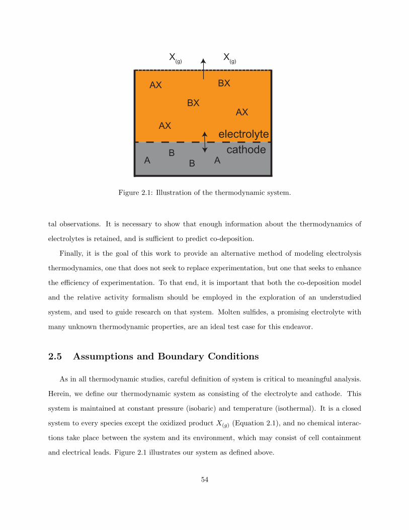
cathodeelectrolyte
X(g)X(g)
A ABB
BX
BX
AX
AXAX
Figure 2.1: Illustration of the thermodynamic system.
tal observations. It is necessary to show that enough information about the thermodynamics of
electrolytes is retained, and is sufficient to predict co-deposition.
Finally, it is the goal of this work to provide an alternative method of modeling electrolysis
thermodynamics, one that does not seek to replace experimentation, but one that seeks to enhance
the efficiency of experimentation. To that end, it is important that both the co-deposition model
and the relative activity formalism should be employed in the exploration of an understudied
system, and used to guide research on that system. Molten sulfides, a promising electrolyte with
many unknown thermodynamic properties, are an ideal test case for this endeavor.
2.5 Assumptions and Boundary Conditions
As in all thermodynamic studies, careful definition of system is critical to meaningful analysis.
Herein, we define our thermodynamic system as consisting of the electrolyte and cathode. This
system is maintained at constant pressure (isobaric) and temperature (isothermal). It is a closed
system to every species except the oxidized product X(g) (Equation 2.1), and no chemical interac-
tions take place between the system and its environment, which may consist of cell containment
and electrical leads. Figure 2.1 illustrates our system as defined above.
54

Considering the electrolyte, it is assumed herein to be a single-phase liquid solution. There are
no conditions on the number of components the electrolyte may contain, and the anode species is
likewise left generalized in order to accommodate many different systems. Importantly, however,
this work lays the groundwork for a model for binary codeposition. Therefore, although the elec-
trolyte may contain more than two components, only two components are considered capable of
reduction (henceforth referred to as species A and B). All other species are modeled as belonging
to the supporting electrolyte, where they are stable enough not to contribute meaningfully to any
reaction. Expansion of this boundary condition will be detailed in Chapter 8.
Analogously, the metal cathode may also be modeled as multicomponent. Unlike the electrolyte,
the solution may contain any number of condensed phases so long as the Gibbs phase rule is
observed. Like the electrolyte, however, any additional species present in the electrolyte beyond A
and B are considered stable and non-reacting.
Finally, contrary to traditional electrochemical convention, all energies of reaction will be nor-
malized per mole of reduced metal. While it is true that electrochemical engineers typically nor-
malize per mole of oxidized gas, the model presented in this thesis focuses on the interactions of
a metallic cathode and liquid electrolyte. Therefore this convention was chosen for mathematical
simplicity.
2.6 Summary
Although it is well-established that electrolyte chemistry is fundamental to the performance of
electrochemical cells, a quantitative link between electrolyte properties and the final composition
of the metal produced at the cathode remains elusive. Furthermore, electrolytes used in high
temperature processes are often reactive- making gathering uncontaminated experimental data
challenging. Because these same electrolytes are usually complex multicomponent solutions, the
ability to model them with traditional thermodynamic computation methods is severely hindered,
mostly due to the increased role of entropy in these systems and the difficulty these methods have
in accurately modeling entropy.
55

It is hypothesized that by examining the equilibrium between the electrolyte and cathode solu-
tions, further insights may be gained about which reduction reactions will dominate in an electro-
chemical cell. The drive for the cell to reach this equilibrium will influence which species will be
reduced and when, and therefore these reactions may be predicted by modeling the thermodynamic
interactions between the electrolyte and cathode.
It is further hypothesized that, in cases where the highly reactive nature of an electrolyte make
direct activity measurements difficult, relative activity measurements between the two species being
evaluated for codeposition is sufficient.
Framework for evaluating these hypotheses has been put forth, and will involve:
1. comparison of the proposed model to experimental data for multiple electrochemical systems
with different anodic species (e.g. oxides, chlorides)
2. development of a mathematical method to rigorously define relative activity in a manner
useful to thermodynamic endeavors
3. measurement of relative activity and critical evaluation of the utility of the results
4. use of relative activity together with the proposed model to probe the properties of molten
sulfides
Validation of these hypotheses would enable development of a model to predict if co-deposition
will occur in an electrochemical cell, and to what extent. Such a model could be utilized by the
electrochemist, not as a replacement for experimentation, as other thermodynamic models often
aim to do, but as a way to quickly screen new systems for feasibility, and as a guide for design of
more efficient and targeted experiments.
56

Bibliography
[1] Alessandro Volta. “XVII. On the electricity excited by the mere contact of conducting sub-
stances of different kinds.” In: Phil. Trans. R. Soc. Lond. 90 (1800), pp. 403–431. url: http:
//rstl.royalsocietypublishing.org/.
[2] G. Kaptay. “The conversion of phase diagrams of solid solution type into electrochemical
synthesis diagrams for binary metallic systems on inert cathodes”. In: Electrochimica Acta
60 (Jan. 2012), pp. 401–409. issn: 00134686. doi: 10.1016/j.electacta.2011.11.077.
[3] James Metson. “Production of Alumina”. In: Fundamentals of Aluminum Metallurgy. Ed. by
Roger Lumley. Cambridge: Woodhead, 2011. Chap. 2, pp. 23–48. isbn: 978-1-84569-654-2.
[4] W.G Davenport et al. Extractive Metallurgy of Copper. Fourth. Elsevier Science, 2002. isbn:
0-444-50206-8.
[5] C.W. Bale et al. “FactSage thermochemical software and databases — recent developments”.
In: Calphad 33.2 (June 2009), pp. 295–311. issn: 0364-5916. doi: 10.1016/J.CALPHAD.2008.
09.009.
[6] A. N. Baraboshkin. Elektrocrystalization from Molten Salts. Moscow: Nauka, 1976.
[7] O. Kubaschewski and Phil Habil. “Application of Chemical Thermodynamics to Practical
Problems”. In: Symposium on the Thermodynamics of High-Temperature Systems. Vol. 60.
Stoke-on-Trent: British Ceramic Society, 1961, pp. 67–83. isbn: 1111111111. doi: 10.1080/
10643389.2012.728825.
57

[8] H Kvande. “Production of Primary Aluminum”. In: Fundamentals of Aluminum Metal-
lurgy. Ed. by Roger Lumley. 1st ed. Woodhead Publishing, 2010. Chap. 3, pp. 49–69. isbn:
9781845696542.
[9] Ksenija Milicevic, Dominic Feldhaus, and Bernd Friedrich. “Conditions and mechanisms of
gas emissions from didymium electrolysis and its process control”. In: Minerals, Metals and
Materials Series. Vol. Part F4. Springer International Publishing, 2018, pp. 1435–1441. isbn:
9783319722832. doi: 10.1007/978-3-319-72284-9_187.
[10] Antony Cox and Derek Fray. “Separation of Mg and Mn from Beverage Can Scrap using a
Recessed-Channel Cell”. In: Journal of The Electrochemical Society 150.12 (2003), pp. D200–
8. doi: 10.1149/1.1623768.
[11] Timothy Lichtenstein et al. “Electrochemical deposition of alkaline-earth elements (Sr and Ba)
from LiCl-KCl-SrCl 2 -BaCl 2 solution using a liquid bismuth electrode”. In: Electrochimica
Acta 281 (Aug. 2018), pp. 810–815. issn: 00134686. doi: 10.1016/j.electacta.2018.05.
097.
[12] John P Ackerman. “Chemical Basis for Pyrochemical Reprocessing of Nuclear Fuel”. In: Ind.
Eng. Chem. Res. 30.1 (1991), pp. 141–5. url: https://pubs.acs.org/sharingguidelines.
[13] John P. Ackerman and Jack L. Settle. “Distribution of plutonium, americium, and several rare
earth fission product elements between liquid cadmium and LiCl-KCl eutectic”. In: Journal
of Alloys and Compounds 199 (Sept. 1993), pp. 77–84. issn: 09258388. doi: 10.1016/0925-
8388(93)90430-U.
[14] Y Sakamura et al. “Distribution behavior of plutonium and americium in LiCl–KCl eutec-
tic/liquid cadmium systems”. In: Journal of Alloys and Compounds 321 (May 2001), pp. 76–
83. issn: 09258388. doi: 10.1016/S0925-8388(01)00973-2.
58
Chapter 3
Mathematical Framework for Linking
Electrolyte Properties to Reduction
Behavior
In Chapter 2, I put forth the hypothesis that an electrolytic cell can be thought of as two
solutions seeking equilibrium with one another- the electrolyte and the cathode. The equilibrium
composition that both solutions want to achieve will define the limits of how the cell can operate.
This concept is familiar to the electrochemist. For example, if one wanted to deposit metallic
aluminum from an aqueous electrolyte, they would decompose water and create hydrogen long
before they could reduce aluminum ions [1]. The reason for this is simple- aluminum oxide is more
thermodynamically stable than water.
Understanding the thermodynamic limitations of an electrolytic cell becomes more complex
once additional chemical reactions become possible and interactions beyond that of pure elements
and compounds start to arise. In such cases, the thermodynamics of electrolysis can no longer be
approximated to the standard state, and solution behavior must be accounted for. In this chapter,
we put forth a mathematical framework for evaluating such solution behavior, and use the insights
gained to obtain further information about the electrolytic cell.
59

3.1 Introduction
The development of the CALPHAD method brought significant advances in the world of creat-
ing computer-generated phase diagrams. Minimization algorithms could compute the equilibrium
of multicomponent systems and map out their phase relations. However, in terms of visualizing
thermodynamics, not much progress has been made since the development of Pourbaix and Elling-
ham diagrams in the 1940’s [2, 3]. Both of these diagrams may be used to compare Gibbs energies
of reactions of different species, and both visualize how certain conditions effect these reaction
energies- in Ellingham’s case, temperature and partial pressure, and in Pourbaix’s case, cell poten-
tial and pH. The derivations of both diagrams, however, make the assumption that the condensed
species taking part in the reaction are in their standard state. In certain cases, this assumption
has led to discrepancies between reaction energies calculated theoretically and those observed ex-
perimentally when standard state behavior does not apply. For example, different solubilities for
oxygen among reactive metals will effect which oxide species is more thermodynamically stable [4].
In his paper “The conversion of phase diagrams of solid solution type into electrochemical syn-
thesis diagrams for binary metallic systems on inert cathodes”, G. Kaptay proposed a type of phase
diagram, called an “equilibrium electrochemical synthesis diagram” (EESD), which links the equi-
librium relationship between metals in the cathode to the reduction potential of the electrolyte [5].
This type of phase diagram is distinct from Pourbaix and Ellingham diagrams because it takes
into account the non-standard state behavior of the metal cathode. No comment is made on the
behavior of electrolytes, which are left generalized. Kaptay’s work focused on the theoretical aspect
of EESD derivation, which he derived for an ideal binary solution only, although equations were
also shown regarding application to real solutions.
In this chapter, the formalism of Kaptay will be extended and expanded to a multicompo-
nent cathode displaying real (ai 6= xi) solution behavior. Through this methodology, targeted
experimental data and classical Gibbs energy curves can be used in combination to map out the
thermodynamic nature of complex electrolytes. To facilitate this effort, a new thermodynamic ref-
erence state for activity is derived that allows one to determine electrolyte activities directly from
60
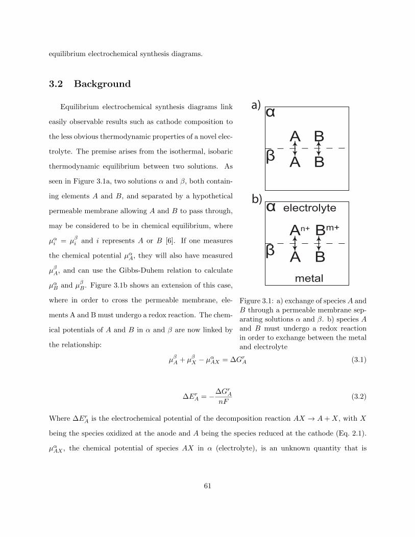
equilibrium electrochemical synthesis diagrams.
3.2 Background
α
βΑ
Α Β
Β
electrolyte
An+
Α Β
Bm+
metal
α
β
a)
b)
Figure 3.1: a) exchange of species A andB through a permeable membrane sep-arating solutions α and β. b) species Aand B must undergo a redox reactionin order to exchange between the metaland electrolyte
Equilibrium electrochemical synthesis diagrams link
easily observable results such as cathode composition to
the less obvious thermodynamic properties of a novel elec-
trolyte. The premise arises from the isothermal, isobaric
thermodynamic equilibrium between two solutions. As
seen in Figure 3.1a, two solutions α and β, both contain-
ing elements A and B, and separated by a hypothetical
permeable membrane allowing A and B to pass through,
may be considered to be in chemical equilibrium, where
µαi = µβi and i represents A or B [6]. If one measures
the chemical potential µαA, they will also have measured
µβA, and can use the Gibbs-Duhem relation to calculate
µαB and µβB. Figure 3.1b shows an extension of this case,
where in order to cross the permeable membrane, ele-
ments A and B must undergo a redox reaction. The chem-
ical potentials of A and B in α and β are now linked by
the relationship:
µβA + µβX − µαAX = ∆GrA (3.1)
∆ErA = −∆GrAnF
(3.2)
Where ∆ErA is the electrochemical potential of the decomposition reaction AX → A+X, with X
being the species oxidized at the anode and A being the species reduced at the cathode (Eq. 2.1).
µαAX , the chemical potential of species AX in α (electrolyte), is an unknown quantity that is
61

a function of two independent variables, µβA and ∆Er. With two unknowns and one equation
(Equation 3.1), µαAX cannot be determined. If the second species, B, is reducing as well, then there
will be a unique potential ES at which the co-reduction of both elements A and B takes place, as
shown in Figure 3.2. If the mixing of A and B are energetically favored, then co-reduction of A
and B will lower the Gibbs energy of reaction such that ES takes place at a more positive potential
than either EA or EB alone. By taking this mixing behavior into account, it is possible to link the
difference between ErA and ErB to the ∆GmixA,B in β (cathode). The derivation of this relationship is
given in [5], and leads to:
∆ES =xB ∗ nB ∗ F ∗∆EB −∆GmixA,B
F [xBnB + (1− xB)nA](3.3)
where ∆EB = EB − EA, (i.e. the difference between B and A on the electrochemical series),
∆ES = ES − EA, and ni are the number of electrons required to reduce i.
If ∆ES is maximized as a function of concentration of A and B in the cathode, and A and B are
assumed to form an ideal solution as metals, ∆EB can be determined directly as a function of the
cathode composition, written here in terms of xB:
∆EB =RT
nAnBF
[nB lnxB − nA ln (1− xB)
](3.4)
This relationship is undoubtedly powerful in linking the alloying chemistries of the cathode to the
properties of an unknown electrolyte, here represented by ∆EB. However, it is limited to cathodes
that form only ideal solutions and are comprised of only A and B. In order to account for a full
range of possible behavior, including phase separation between A and B and the use of additional
“host” metals in the cathode, the derivation should generalized. Herein, this relationship will
be re-derived for the general case of a multicomponent cathode behaving as a real solution with
aB 6= xB.
62
3.3 Derivation of Generalized Model
Consider a ternary system of three elements: A, B, C. Elements A and B can be reduced from
the electrolyte into the cathode, while element C is a stable cathode host and does not interact
with the electrolyte. The concentration of A, the more noble element, is taken as the dependent
variable so concentration can be reframed in terms of B and C only. In addition, although for this
derivation C is assumed to be a single element (the cathode is modeled as three components), C
can also be any compound or alloy of fixed concentration, as long as it does not contain either A
or B. The Gibbs energy of mixing A, B, and C to produce a liquid cathode is given by:
∆Gmix = Gl − (1− xB − xC)G0A − xBG0
B − xCG0C (3.5)
G0i is the standard state Gibbs energy of pure element i at the temperature and pressure of elec-
trolysis. Gl is the Gibbs energy of a liquid cathode phase created by alloying A, B, and C. It can
be represented by
(1− xB − xC)GlA + xBGlB + xCG
lC +RT [(1− xB − xC) ln aA + xB ln aB + xC ln aC ] (3.6)
Where Gli is the Gibbs energy of element i in the pure liquid state. 1.
Element A reduces at cathode potential EA, B at EB, and both will co-reduce at a common
potential ES (Figure 3.2). Following the convention of Kaptay, A is a more “noble” species than
B, reducing at less negative potentials [5].
If mixing is favorable, there will be an energetic drive for A and B to reduce together at ES .
The shift from EA (or EB) to ES can therefore be directly equated to the contribution of A and B
to the Gibbs energy of mixing:
∆Gmix = −xBnBF (ES − EB)− (1− xB − xC)nAF (ES − EA) + xC∆GmixC (3.7)
1If pure i is liquid at the temperature of interest, Gi = Gli. If pure i is solid, but forms a liquid solution with a
cathode alloy, Gi 6= Gli
63

Eref
ES
EA
EB
E vs. Eref/V
ΔE S
ΔE Β
Figure 3.2: Hypothetical placement of EA, EB, and ES on electrochemical potential series. In thisexample, Eref = 0.
where
∆GmixC = GlC +RT ln aC −G0C (3.8)
and ni is the number of electrons necessary to reduce species i, as in Equations 2.1 - 2.2. We can
expand and then simplify Equation 3.7 with the relations ∆EB = EB −EA and ∆ES = ES −EA,
as illustrated in Figure 3.2. This leads to:
∆Gmix = −xBnBFES + xBnBFEB − (1− xB − xC)nAF (∆ES) + xC∆GmixC +
+(xBnBFEA − xBnBFEA)
(3.9)
∆Gmix = −xBnBF∆ES + xBnBF∆EB − (1− xB − xC)nAF (∆ES) + xC∆GmixC (3.10)
64
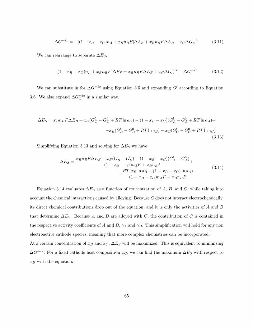
∆Gmix = −[(1− xB − xC)nA + xBnBF ]∆ES + xBnBF∆EB + xC∆GmixC (3.11)
We can rearrange to separate ∆ES :
[(1− xB − xC)nA + xBnBF ]∆ES = xBnBF∆EB + xC∆GmixC −∆Gmix (3.12)
We can substitute in for ∆Gmix using Equation 3.5 and expanding Gl according to Equation
3.6. We also expand ∆GmixC in a similar way.
∆ES = xBnBF∆EB + xC(GlC −G0C +RT ln aC)− (1− xB − xC)(GlA −G0
A +RT ln aA)+
−xB(GlB −G0B +RT ln aB)− xC(GlC −G0
C +RT ln aC)
(3.13)
Simplifying Equation 3.13 and solving for ∆ES we have
∆ES =xBnBF∆EB − xB(GlB −G0
B)− (1− xB − xC)(GlA −G0A)
(1− xB − xC)nAF + xBnBF+
−RT (xB ln aB + (1− xB − xC) ln aA)
(1− xB − xC)nAF + xBnBF
(3.14)
Equation 3.14 evaluates ∆ES as a function of concentration of A, B, and C, while taking into
account the chemical interactions caused by alloying. Because C does not interact electrochemically,
its direct chemical contributions drop out of the equation, and it is only the activities of A and B
that determine ∆ES . Because A and B are alloyed with C, the contribution of C is contained in
the respective activity coefficients of A and B, γA and γB. This simplification will hold for any non
electroactive cathode species, meaning that more complex chemistries can be incorporated.
At a certain concentration of xB and xC , ∆ES will be maximized. This is equivalent to minimizing
∆Gmix. For a fixed cathode host composition xC , we can find the maximum ∆ES with respect to
xB with the equation:
65

∂∆ES∂xB
)xC
= 0 (3.15)
Solving for ∆EB and simplifying gives:
∆EB =nA∆GssB − nB∆GssA − nBRT ln[(1− xB − xC)γA] +RT ln[xBγB]
FnAnB(3.16)
Where ∆Gssi refers to the change in energy when moving from the standard state of species i
at a given T to a liquid state. This is the generalized version of Equation 3.4 that can be applied
to any liquid cathode chemistry. It details how the composition of the cathode can influence the
extent of co-deposition. When plotting xB against ∆EB, an equilibrium electrochemical synthesis
diagram is created. For clarity of plotting, xB is better plotted against −∆EB. In this notation,
more positive potential differences favor the element A with a more positive potential. In order
to facilitate comparison with other equilibrium diagrams (e.g. phase diagrams), the EESD’s in
this paper are rotated from the original design of Kaptay, placing concentration on the x-axis. An
example of an electrochemical synthesis diagram plotted in this way for a general system A and B
at temperature T is given in Figure 3.3.
Equilibrium electrochemical synthesis diagrams provide a quantitative relationship between
two metals’ willingness to alloy in the cathode and the difference in the electrochemical potentials
required to reduce them. Two metals with favorable mixing properties, such as Pr and Nd, will
have a very steep curve, indicating that very large potential differences |∆EB| >> 0 are needed
to avoid codeposition (Figure 3.4). On the contrary, two metals that phase separate, such as
Ni and Ag, will have a horizontal curve in the region of phase separation, and a much shallower
curve overall (Figure 3.5). This indicates that for there to be significant codeposition, ∆EB ≈ 0.
The tendencies of Ni and Ag to avoid mixing in the cathode result in a higher energetic barrier to
codeposition. This EESD indicates it is far easier to electrochemically separate Ag from Ni in a
molten salt than it would be to separate Pr from Nd.
To construct a simple EESD, this potential difference, ∆EB, is left generalized. Looking in
more detail, we see ∆EB is a function of the standard state electrochemical potentials of A and B,
66

A BxB
Ε A- Ε
B(V)
Figure 3.3: Equilibrium electrochemical synthesis diagram for arbitrary binary A-B, where A isthe more noble element on the electrochemical potential series, and A and B form a completelymiscible metallic solution.
as well as their activity in the electrolyte, here designated by the notation aAX and aBX , where X
is the anionic species in the electrolyte. We have:
−∆EB = EA − EB = EA −RT
nAFln aAX − (EB −
RT
nBFln aBX) (3.17)
Although in most cases, the standard state electrochemical potentials EA and EB are known,
the activities aAX and aBX are often unknown. Direct experimental measurement of activity is
possible, but difficult if co-deposition of A and B is favored. In this case an ion-selective membrane
must be used. If the supporting electrolyte reacts with either the membrane or the reference, the
67
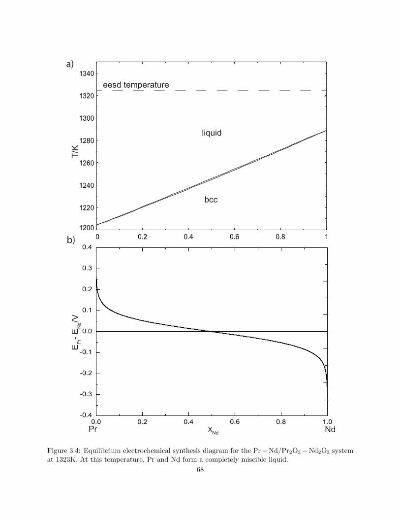
0 0.2 0.4 0.6 0.8 11200
1220
1240
1260
1280
1300
1320
1340
Pr Nd
bcc
liquid
T/K
eesd temperature
xNd
a)
b)
Ε Pr- Ε N
d/V
Figure 3.4: Equilibrium electrochemical synthesis diagram for the Pr−Nd/Pr2O3−Nd2O3 systemat 1323K. At this temperature, Pr and Nd form a completely miscible liquid.
68

T/K eesd temperature
liquid 1 + liquid 2
fcc + liquid 1
Ag NixNi
b)
a)
liqui
d 1 liquid 2
Ε Ag- Ε N
i/V
Figure 3.5: Equilibrium electrochemical synthesis diagram for the Ag− Ni/AgCl2 − NiCl2 systemat 1773K. At this temperature, Ag and Ni phase separate to form two different liquid solutions.
69
activity measurements will be contaminated. Unfortunately, many high-temperature supporting
electrolytes are highly reactive, and a compatible membrane or reference may not be available.
3.4 The Case for a New Reference State
Thermodynamic convention calls for the study of relative changes in the energy of a system:
absolute values of energy and enthalpy are not necessary within a classical framework. The energy
of the initial state of matter, then, can be chosen according to the convenience of the thermody-
namicist, as long as they remain consistent throughout their calculations.
In the equation for molar Gibbs energy,
Gi = µi = µoi (T ) +RT ln ai (3.18)
µoi is defined arbitrarily according to mathematical and experimental convenience. When ai → 1,
species i is said to be in its standard state, and µi = µoi . The deviation of the activity function
ai from unity can thus be thought of as a measurement of deviation from standard state. This
deviation may be viewed as a function of the concentration of i in a multicomponent system:
ai = xiγi, where γi is called the activity coefficient, and is the activity of species i normalized by
its concentration. When γi = 1, ai = xi and the material is said to behave ideally. When γi > 1,
ai > xi and µi > µoi and i is in a state with elevated Gibbs energy relative to its standard state.
If µoi is defined to represent the energetic state of i as a pure substance in its thermodynamically
stable phase at standard pressure (1 atm), then this behavior may be interpreted as an increase in
free energy upon mixing into a multicomponent system. If the increase in energy upon mixing is
high enough, phase separation will occur. Conversely, when γi < 1, ai < xi and µi < µoi and i is
in a state with lowered Gibbs energy relative to its standard state. The system favors interaction
between i and the other components in the system. If the interactions lower the energy sufficiently,
short range ordering and, in some cases, compound formation, will occur.
Two main reference states exist for relating the activity function to the chemical potential.
70
The first, and by far the most common in thermodynamics, is the Raoultian reference state. In a
Raoultian reference state:
γixi→1 = 1 (3.19)
In other words, the reference state is chosen to be one where Raoult’s law applies.
In contrast, in a Henrian reference state, the reference state is chosen to be where Henry’s law
applies:
fixi→0 = 1 (3.20)
where f is the Henrian activity coefficient.
No matter the reference state, the integral chemical potential µi does not change. Activity
framed in one reference state may be easily converted to another by a proportionality factor in-
dependent of concentration [7]. In both of these reference states, ai is quantified, and all other
activities aj can be found by Gibbs-Duhem integration. This is valid no matter how many compo-
nents the system contains.
In certain cases, it is difficult to measure the activity of species i independently. Molten sulfides,
highly reactive at elevated temperatures, are one such case, and others have been discussed in
Chapter 1. Fortunately, in order to predict the extent of co-reduction between two electroactive
species, independent activities are not necessary. It is the relative difference between the activities of
two electroactive species AX andBX that determine their relative placement on the electrochemical
series, and this in turn dictates which species will be reduced first.
3.4.1 The Wagner-Allanore Reference State
Herein, we propose a third reference state, the Wagner-Allanore reference state. This reference
state is derived specifically for multicomponent solutions where direct activity measurements are
difficult. It is a relative reference state where the activities of two species dissolved in a complex
solvent are measured relative to one another (e.g. two electroactive species in a multicomponent
71
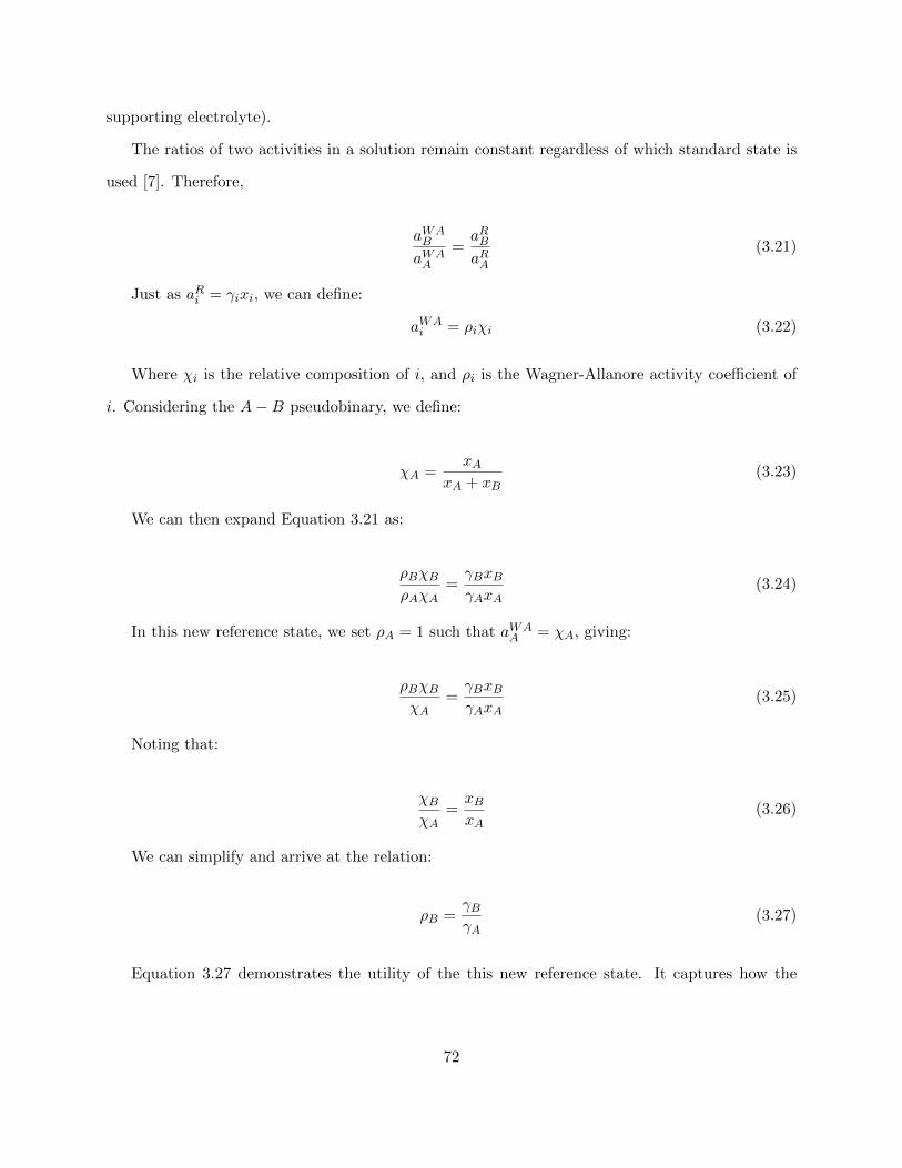
supporting electrolyte).
The ratios of two activities in a solution remain constant regardless of which standard state is
used [7]. Therefore,
aWAB
aWAA
=aRBaRA
(3.21)
Just as aRi = γixi, we can define:
aWAi = ρiχi (3.22)
Where χi is the relative composition of i, and ρi is the Wagner-Allanore activity coefficient of
i. Considering the A−B pseudobinary, we define:
χA =xA
xA + xB(3.23)
We can then expand Equation 3.21 as:
ρBχBρAχA
=γBxBγAxA
(3.24)
In this new reference state, we set ρA = 1 such that aWAA = χA, giving:
ρBχBχA
=γBxBγAxA
(3.25)
Noting that:
χBχA
=xBxA
(3.26)
We can simplify and arrive at the relation:
ρB =γBγA
(3.27)
Equation 3.27 demonstrates the utility of the this new reference state. It captures how the
72
chemical potential of species A and B vary with respect to each other, as well as how other
components in the solution may effect this relationship. For example, if A and B are dissolved into
solvent C, and solvent C tends to bond with A (γA < 1), while phase separating with B (γB > 1),
then γB > γA and ρB > 1. In certain cases, exact calculation of γA and γB is impractical or difficult,
but ρB can be easily measured by using an EESD diagram in combination with Equation 3.17. Since
ρB is all that is needed to determine if the electrolyte solution properties favor codeposition or
purification, reframing activity in this reference state is particularly useful to electrochemists. The
Wagner-Allanore reference state can be converted to a Raoultian reference state via the equation:
aRB = aWAB γA (3.28)
The conversion factor, γA is a function of composition xA. Because the composition coordinate
χ is relative as well, there are no limits on how dilute or concentrated A and B can be in the
solvent. Thus, this new reference state has several significant advantages over Raoultian and Hen-
rian states. First, because it is a relative reference state, not an absolute reference, it is easier to
measure experimentally, particularly when very reactive solutions are involved. Second, because it
measures the pseudobinary between A and B, there are no conditions on concentration. A Raoul-
tian reference state is the simplest mathematically and experimentally when a material is very
concentrated. A Henrian reference state is the simplest mathematically and experimentally when
a material is very dilute. By defining a new composition coordinate χ, species A and B can be at
any dilution. Although the exact, independent activities of A or B cannot be determined, and thus
Gibbs-Duhem integration cannot be performed, much of the information about the solution is still
retained, such as how A and B interact with each other and with their solvent. Figure 3.6 shows
a comparison between activities reported in a Raoultian, Henrian, and Wagner-Allanore reference
state.
73
0.2 0.4 0.6 0.80 1
∞
A
1
1
1∞
aR aH
xBB
0 0.5 1
1
aWA
Figure 3.6: Comparison of Raoultian, Henrian, and Wagner-Allanore reference states. Henrianactivities are scaled according to the value of γ∞, while Wagner-Allanore activities are scaledaccording to the activity coefficient of A, γA, which may not be constant with concentration,unlike the Henrian case. The composition coordinate of the Wagner-Allanore reference state is alsorescaled along the A−B pseudobinary.
74

3.5 Summary
Re-framing activity in a relative framework is advantageous for the study of electrolytes with
activities difficult to measure directly. In combination with equilibrium electrochemical synthesis
diagrams, relative activity can be measured after equilibrating the cathode and electrolyte, as long
as the activity of the cathode has been previously determined. Fortunately, many metallic systems
have previously been studied in detail, and this information is readily available.
As will be shown in the following chapters, significant information about electrolytes can be
obtained with this method, even if direct activity is never measured. Such information can be used
to drive the design of further electrochemical experiments, as well as to quickly screen systems for
their limitations. For example, achieving a pure cathode product when two metals have a strong
Gibbs energy of mixing will be challenging, and if their ∆EB is small for a chosen electrolyte, it
may not be possible. In such cases, it will be apparent from an EESD that alternative methods
should be pursued. This valuable information for the electrochemist can now be realized far more
quickly, as only a few experiments in tandem with an EESD are required for this analysis.
Currently, the model for EESD’s have been only derived for comparison of two species in the
electrolyte (binary system). Direct comparison of three species is possible, but this would require
a third axis and would produce a three-dimensional figure similar to a complete (non-isothermal)
ternary phase diagram. It is simpler to compare three species indirectly, by first measuring ρB,
the activity coefficient relative to A, and then by measuring a third component relative to A, for
example ρD (recall that C is a non-interacting cathode specie), but this assumes negligible ternary
interactions between A, B, and D. A full discussion of possible extensions of this model is given in
Chapter 8.
75
Bibliography
[1] Allen J. Bard and Larry R. Faulkner. Electrochemical Methods- Fundamentals and Applica-
tions. Second. J. Wiley, 2001. isbn: ISBN 0-471-04372-9.
[2] M. Pourbaix. “Thermodynamique des solutions aqueuses diluees: Representation graphique
du role du pH et du potentiel”. PhD thesis. Technical University Delft, 1945.
[3] H.J.T. Ellingham. “Reducibility of Oxides and Sulphides in Metallurgical Processes”. In:
Journal of the Society of Chemical Industry 63.5 (May 1944), p. 133. issn: 03684075. doi:
10.1002/jctb.5000630501.
[4] O. Kubaschewski and Phil Habil. “Application of Chemical Thermodynamics to Practical
Problems”. In: Symposium on the Thermodynamics of High-Temperature Systems. Vol. 60.
Stoke-on-Trent: British Ceramic Society, 1961, pp. 67–83. isbn: 1111111111. doi: 10.1080/
10643389.2012.728825.
[5] G. Kaptay. “The conversion of phase diagrams of solid solution type into electrochemical
synthesis diagrams for binary metallic systems on inert cathodes”. In: Electrochimica Acta
60 (Jan. 2012), pp. 401–409. issn: 00134686. doi: 10.1016/j.electacta.2011.11.077.
[6] L.S. Palatnik and A.I. Landau. Phase Equilibria in Multicomponent Systems. Ed. by Joseph
Joffe. New York: Holt, Rinehart, and Winston, Inc., 1964.
[7] C H P Lupis. Chemical Thermodynamics of Materials. New York: North-Holland, 1983. isbn:
9780444007797.
76

Chapter 4
Modeling Case Studies in Industrial
Electrochemistry
Although production of a pure metal through electrolysis is typically achieved by using a pure
feedstock or selective solvent, there are certain cases where two species are soluble and present
in amounts that make co-deposition possible (see Chapter 1). One such case is nuclear waste
processing, where due to the radioactive nature of the components, multiple pre-purifying steps
prior to electrolysis introduce radiation contamination risks and are thus impractical. As such,
significant efforts have been expended towards investigating recycling metals from nuclear waste
in one single electrolytic cell [1–3]. In this chapter, I will investigate the separation of cobalt from
nickel in a molten chloride media, and compare model results and insights to the experimental
analysis given in [4].
Another notable system for industrial co-depositon is rare earth alloy production. Although
individual rare earths are usually produced as pure metals via electrolysis after extensive pre-
processing to ensure a pure oxide feedstock [5–7], occasionally neodymium and praseodymium are
electrolyzed together to produce a Pr-Nd alloy [8, 9]. Due to the near-exclusive production of rare
earth metals in China, little information on the actual process conditions of rare earth electrolysis
have spread beyond a select few Chinese companies, where such information is closely held as
trade secrets [7, 10]. Some published data are available, but they lack key details crucial to the
77
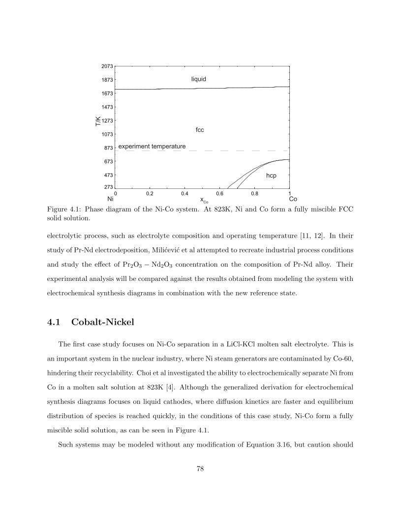
0 0.2 0.4 0.6 0.8 1273
473
673
873
1073
1273
1473
1673
1873
2073
T/K
Ni xCo Co
fcc
experiment temperature
liquid
hcp
Figure 4.1: Phase diagram of the Ni-Co system. At 823K, Ni and Co form a fully miscible FCCsolid solution.
electrolytic process, such as electrolyte composition and operating temperature [11, 12]. In their
study of Pr-Nd electrodeposition, Milicevic et al attempted to recreate industrial process conditions
and study the effect of Pr2O3 − Nd2O3 concentration on the composition of Pr-Nd alloy. Their
experimental analysis will be compared against the results obtained from modeling the system with
electrochemical synthesis diagrams in combination with the new reference state.
4.1 Cobalt-Nickel
The first case study focuses on Ni-Co separation in a LiCl-KCl molten salt electrolyte. This is
an important system in the nuclear industry, where Ni steam generators are contaminated by Co-60,
hindering their recyclability. Choi et al investigated the ability to electrochemically separate Ni from
Co in a molten salt solution at 823K [4]. Although the generalized derivation for electrochemical
synthesis diagrams focuses on liquid cathodes, where diffusion kinetics are faster and equilibrium
distribution of species is reached quickly, in the conditions of this case study, Ni-Co form a fully
miscible solid solution, as can be seen in Figure 4.1.
Such systems may be modeled without any modification of Equation 3.16, but caution should
78
be used when assuming the EESD is representative of the bulk cathode composition (i.e. assuming
the concentration of Co is sufficiently diffused such that it is uniform throughout the cathode). To
the author’s knowledge, there is no full thermodynamic study of the NiCl2 − CoCl2 − LiCl−KCl
system. CALPHAD models for electrolyte appear to be obtained via extrapolation from similar
chloride systems, rather than from direct measurement [13–19].
4.1.1 Results
Choi et al studied the deposition of Ni-Co alloys with three different concentration ratios of
NiCl2 − CoCl2: 2wt%NiCl2-2wt%CoCl2, 2wt%NiCl2-1wt%CoCl2, and 2wt%NiCl2-0.5wt%CoCl2.
In addition to varying the concentration, electrolysis was run at three different current densities:
50mA, 200mA, and 500mA.
The standard-state decomposition potential of liquid NiCl2 to Ni is -798mV, while the standard-
state decomposition potential of liquid CoCl2 to Co is -998mV. Note that both NiCl2 and CoCl2
are solid in their pure state, yet soluble in liquid LiCl-KCl. For this reason, thermodynamics of the
liquid should be used. The difference in decomposition potential between Ni and Co, ENi − ECo,
is 200mV if NiCl2 and CoCl2 are assumed to behave ideally with respect to each other. On the
electrochemical synthesis diagram shown in Figure 4.2a, a 200mV potential difference corresponds
to approximately 0.25 mol%Co alloyed into the Ni cathode.
In their investigation of reduction potential peaks through cyclic voltammetry, Choi et al mea-
sured a potential difference of 185mV when both NiCl2 and CoCl2 are present each at 2wt% in
the supporting electrolyte [4]. On an electrochemical synthesis diagram, a 185mV difference cor-
responds to approximately 0.37 mol%Co. Chronopotentiometry experiments of this electrolyte
concentration revealed an experimental cathode concentration of 0.22, 0.53, and 1.17 mol%Co for
current densities of 50mA, 200mA, and 500mA, respectively. Figure 4.2b compares the Wagner-
Allanore activity coefficient calculated for each experiment, compared with the predicted coefficient
from the synthesis diagram. There is strong agreement between the predicted activity coefficient
and that measured with a low current density (50mA). As current density increases, the amount
of Co in the Ni cathode increases, and the measured activity coefficient strays from its equilibrium
79
thermodynamic prediction.
Figure 4.3 shows a comparison of the Wagner-Allanore activity coefficient as calculated for
different concentrations of NiCl2 and CoCl2. ρCoCl2 appears to be highly dependent on the cell’s
current density. It can also be seen that as the concentration of CoCl2 in the electrolyte increases,
the amount of Co deposited on the cathode also increases. Increases in Co deposition with current
density also occur for lower concentrations of CoCl2, although they are less pronounced than in
the case where xNiCl2 = xCoCl2 = 2wt%. This effect can be more readily seen in Figure 4.4. When
xCoCl2 = 0.5wt% the difference in Co content in the cathode achieved through electrolysis at 50
mA and 500 mA was ≈ 0.002. In comparison, when xCoCl2 = 2wt%, the difference in Co content
was ≈ 0.01.
If ENi−ECo is calculated with an ideal solution assumption, it will vary with electrolyte compo-
sition. Figure 4.5 shows this ∆Eideal calculated when xCoCl2 = 0.5wt%, 1wt%, and 2wt%, compared
to the corresponding data obtained from electrolysis at 50mA. As in Figure 4.2, there is good agree-
ment between experimental data and model predictions using an ideal solution assumption. Note
that when an ideal solution assumption is used, ρCoCl2 = 1 (see Chapter 3).
4.1.2 Discussion
Figure 4.2 compares the amount of Co predicted in the Ni cathode after electrolysis with
experimental results. The predicted value of 0.25 mol% is calculated using an EESD that relates
ENi − ECo to the thermodynamics of a Ni-Co alloy. Without experimental data, ENi − ECo is
unknown, however, it can be approximated by using an ideal solution model. A liquid standard
state takes into account the change in Gibbs energy upon dissolving solid NiCl2 and CoCl2 into
molten chloride electrolyte. Even when there is no further information available regarding the
electrolyte, using an EESD allows one to take into account the contribution of Ni-Co mixing in
the cathode. The value of this additional information can be seen in the agreement between the
predicted values of Co concentration read off of an EESD using ∆Eideal, and the values achieved
during low current density electrolysis (Figure 4.5).
Focusing on the set of experiments where xCoCl2 = 2wt%, the difference between the measured
80

Ni CoxCo
ρ CoC
l2
Ni CoxCo
a)
b)
200mA
500mA
50mA
ideal solution
CV
CV
idealsolution
50mA
200mA
500mA
Ε Ni- Ε C
o/V
Figure 4.2: a) Electrochemical synthesis diagram for Ni−Co/NiCl2−CoCl2 system at 823K wherexNiCl2 = xCoCl2 = 2wt%. b) Wagner-Allanore activity coefficient ρ for CoCl2. : Values calculatedfor: ENi − ECo = 0.2V (from ideal solution), and ENi − ECo = 0.185V (from cyclic voltammetrypeaks). ;: experimental concentration of Co in Ni cathode after chronopoteniometry at 50mA/cm2,200mA/cm2, and 500mA/cm2 [4].
81

Ni xCo Co
ρ CoC
l2
50mA
500mA500mA 500mA
50mA50mA
200mA
200mA
200mA
Figure 4.3: Wagner-Allanore activity coefficient ρCoCl2 calculated from experimental concentra-tion of Co in Ni cathode after electrolysis at 50mA/cm2, 200mA/cm2, and 500mA/cm2, when
xCoCl2xNiCl2
+xCoCl2= 0.2 (W) , 0.33 (5), and 0.5 (;) [4].
82

500mA
500mA
500mA200mA
200mA
200mA50mA
50mA
50mA
Ni xCo Co
x CoC
l
x NiC
l +
x CoC
l
2
22
Figure 4.4: Comparison of electrolyte composition and cathode concentration after electrolysis at50mA/cm2, 200mA/cm2, and 500mA/cm2, when
xCoCl2xNiCl2
+xCoCl2= 0.2 (W) , 0.33 (5), and 0.5 (;) [4].
83

ρ CoC
l2
Ni xCo Co
ideal solution
ideal solution
ideal solution
0.5 wt%
1 wt% 2 wt%
Figure 4.5: Comparison of ρCoCl2 calculated from experimental concentration of Co in Ni cathodeafter electrolysis at 50mA/cm2, to ideal solution assumption for
xCoCl2xNiCl2
+xCoCl2= 0.2 (W) , 0.33 (5),
and 0.5 (;). Ideal solution model: [4].
84

reduction potentials of Co and Ni during cyclic voltammetry is 225mV, corresponding to 0.37
mol%Co in Ni on an EESD. This is slightly higher than the value predicted by the ideal solution
case, and higher than the composition measured after electrolysis at 50mA. Without data on the
equilibrium exchange between Co and Ni in molten chloride, one cannot determine if this difference
is due to solution interactions or kinetic and mass transport effects that arose during electrochemical
operation. However, there is some evidence to suggest that non-thermodynamic effects play a non-
negligible role in the final experimental result. First, the Ni-Co alloy is solid at 823K, which will
inevitably hinder diffusion of Co into Ni and effect the alloy chemistry. Second, independently of
CoCl2 concentration, there was good agreement between Co content predicted from an ideal solution
assumption and Co content measured after 50 mA electrolysis (Figure 4.5), suggesting that NiCl2
and CoCl2 behave ideally with respect to each other in this system and making additional solution
interactions less likely.
Furthermore, higher current density during electrolysis corresponded to higher experimental
concentrations of Co in the cathode. Higher current densities during electrolysis can push the cell
into an operation regime limited by mass transport. If there is locally increased concentration of
CoCl2 in the vicinity of the cathode, for example, then ρCoCl2 will be higher at the electrode interface
than in the bulk solution. In fact, as current density increased from 50mA to 500mA, calculated
ρCoCl2 was observed to increase correspondingly. Figure 4.3 shows that even as concentration of
CoCl2 is varied, the values of ρCoCl2 remain correlated to current density. When the concentration
of CoCl2 is low, the effect of current density on Co content in the cathode is lessened. If indeed
there are mass-transport limitations present causing gradients in the electrolyte, it is possible that
low CoCl2 concentrations overall prevent large gradients from forming. It is also possible that
other contributions could be at play, and more electrochemical studies would be needed to further
analyze the cell behavior.
85
4.2 Praseodymium-Neodymium
The second case study investigates Pr-Nd alloy production from a mixed rare earth oxide.
This system was selected for several notable reasons. First, Pr-Nd electrolysis takes place in a
molten fluoride electrolyte into which Nd2O3 and Pr2O3 are dissolved. The anion here is the oxide
ion, which is different from the anion of the supporting electrolyte, the fluoride ion. The additional
interactions between the two anions create additional complications that hinder modeling efforts and
frustrate attempts to measure thermodynamic properties. By re-framing the solution properties of
the oxyfluoride electrolyte into the relative Wagner-Allanore reference state, this confusion is easily
avoided and the energetic effect the molten fluoride has on the dissolved oxide species is captured
by ρ. Second, as mentioned previously, the conditions under which Pr-Nd electrolysis take place
are proprietary. Without information about the actual electrolyte composition used, and with
process conditions (temperature, current density, atmosphere) unknown, it is difficult to replicate
the conditions in a laboratory setting in order to gather thermodynamic data. Commercially
available CALPHAD models of the electrolyte are limited to binary fluoride systems, and even
then, available models are extrapolated from the data of better understood systems [20]. An
alternate method of investigating the thermodynamic properties of this electrolyte would clearly
aid researchers in understanding more about Pr-Nd alloy production methods.
4.2.1 Results
The Pr-Nd metallic system is well enough understood to build a binary CALPHAD model (Fig-
ure 3.4), which can be used to generate an electrochemical synthesis diagram for the system. At
1323K, standard state decomposition potential of liquid Pr2O3 to liquid Pr is -2.363V, while the
standard state decomposition potential of liquid Nd2O3 to liquid Nd is -2.372V. For an oxide com-
position ratio 66 mol%Nd2O3 - 33 mol%Pr2O3, potential difference EPr−ENd calculated assuming
ideal solution behavior is -5mV (Figure 4.6). Using an EESD, this corresponds to a Pr-Nd cathode
containing 53.5 mol% Nd. In Milicevic’s experiments, electrolysis from an oxyfluoride containing
66 mol%Nd2O3 - 33 mol%Pr2O3 produced a cathode composition of 71 mol%Nd - 29 mol%Pr
86
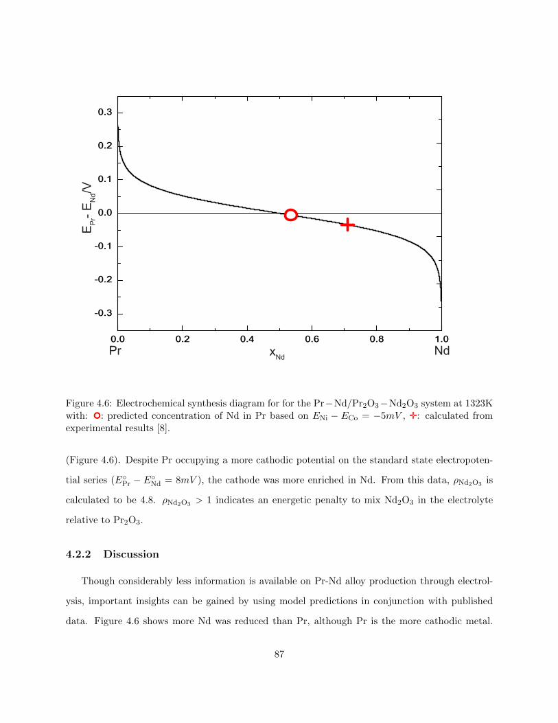
Pr NdxNd
Ε Pr- Ε N
d/V
Figure 4.6: Electrochemical synthesis diagram for for the Pr−Nd/Pr2O3−Nd2O3 system at 1323Kwith: : predicted concentration of Nd in Pr based on ENi − ECo = −5mV , ;: calculated fromexperimental results [8].
(Figure 4.6). Despite Pr occupying a more cathodic potential on the standard state electropoten-
tial series (EPr − ENd = 8mV ), the cathode was more enriched in Nd. From this data, ρNd2O3 is
calculated to be 4.8. ρNd2O3 > 1 indicates an energetic penalty to mix Nd2O3 in the electrolyte
relative to Pr2O3.
4.2.2 Discussion
Though considerably less information is available on Pr-Nd alloy production through electrol-
ysis, important insights can be gained by using model predictions in conjunction with published
data. Figure 4.6 shows more Nd was reduced than Pr, although Pr is the more cathodic metal.
87
Looking at only standard state data, one might expect the cathode to be strongly enriched in Pr.
However, by combining an ideal solution assumption with an EESD, a cathode containing 53.5
mol% Nd is predicted.
Experimentally, even more Nd was obtained via electrolysis: 71 mol% Nd. There are several
reasons why this may have occured. First, from the experimental data, ρNd2O3 ≈ 4.8. If this value
is representative of equilibrium conditions, then there is an energetic penalty for mixing Nd2O3
into the electrolyte, and the original ideal solution assumption would be invalid. Since the value of
this increased Gibbs energy of mixing is measured relative to Pr2O3, it suggests there is a driving
force to reduce the concentration of Nd2O3 in the electrolyte while increasing the concentration of
Pr2O3. This will result in increased production of Nd metal.
An alternative explanation considers that although Pr is the more cathodic metal on the elec-
tropotential series for oxides, Nd is the more cathodic metal for the fluoride series. Both PrF3 and
NdF3 are present in the fluoride supporting electrolyte [9]. If PrF3 and NdF3 were being reduced
preferentially instead of the oxides, a more Nd-rich alloy would be the result. However, in order for
rare earth fluorides to be reduced in steady state, the fluoride ion should be oxidized at the anode,
typically producing perfluorinated compounds (PFC) when the electrolyte is a molten oxyfluoride.
Literature studying PFC emissions in Pr-Nd electrolysis cells have noted that they are on average
2-3 orders of magnitude lower than CO2 production [9, 12]. Even if all PFC emissions were the
result of NdF3 electrolysis, there would not be enough Nd produced from fluoride to account for
the change in cathode composition.
A final explanation for the increased production of Nd could be the result of mass transport
limitations inside the electrolysis cell. Nd2O3 is present at nearly double the concentration of
Pr2O3. At the high current densities used for electrolysis, it is entirely plausible that in the vicinity
of the cathode, there was an even greater concentration difference between Nd2O3 and Pr3O3 [9].
This explanation concurs with the results of the Ni-Co case, where deposition of Co was noted to
increase with current density. Furthermore, available thermodynamic models for the LiF − PrF3
system and the LiF−NdF3 system suggest Nd and Pr behave similarly with respect to each other
in the electrolyte [20], which would result in an equilibrium ρ ≈ 1 and support the validity of an
88
ideal solution assumption. It is critical to note, however, that this is only for the thermodynamics
of the molten fluorides. To the author’s knowledge, there is currently no commercially available
thermodynamic data, experimental or modeled, for the Pr−Nd−O system. Further experimental
investigation is necessary in order to determine if Nd enrichment in the electrolyte is the result of
thermodynamic or transport phenomena.
4.3 Summary
In both the Ni-Co and Pr-Nd case studies, analyzing existing data with equilibrium electro-
chemical synthesis diagrams provided new information about the system. In addition, reframing
activity in our new relative reference state allowed for the electrolyte thermodynamics to be inves-
tigated and new information obtained. Available CALPHAD models for the Ni-Co case appear to
be derived from extrapolation and comparison to similar systems, while with the exact electrolyte
composition of the Pr-Nd oxyfluoride unknown, no activity measurements are publicly available.
The model for predicting co-deposition presented above enables the electrochemist to make use
of incomplete and scattered data. Unlike the CALPHAD method, where large amounts of data at
various conditions are necessary to build a model, data from only one experiment (as in the Pr-Nd
case) can provide valuable information about electrolysis as long as the cathode thermodynamics
are known. If no data is available, generalized EESD’s allow one to account for the effect cathode
chemistry has on co-deposition. Using this information alongside a simple model for the electrolyte
(e.g. ideal solution) can predict results close to experimental outcome (Figure 4.5, Figure 4.6).
In addition to allowing further analysis of an electrochemical system where limited data might
have prevented such efforts in the past, the co-deposition model and new reference state also
increase the information that can be obtained from experiments. In the Ni-Co case study, for
example, chronopotentiometry experiments at various current densities show the effect that non-
thermodynamic effects can have on the alloy produced during electrolysis. Thus, although EESD’s
are an equilibrium diagram, they may also be utilized to interpret kinetic effects to a limited extent.
A discussion of model expansion beyond thermodynamics is given in Chapter 8.
89
Bibliography
[1] John P. Ackerman and William E. Miller. Electrorefining process and apparatus for recovery
of uranium and a mixture of uranium and plutonium from spent fuels. Nov. 1989.
[2] John P Ackerman. “Chemical Basis for Pyrochemical Reprocessing of Nuclear Fuel”. In: Ind.
Eng. Chem. Res. 30.1 (1991), pp. 141–5. url: https://pubs.acs.org/sharingguidelines.
[3] John P. Ackerman and Jack L. Settle. “Partition of lanthanum and neodymium metals and
chloride salts between molten cadmium and molten LiCl-KCl eutectic”. In: Journal of Alloys
and Compounds 177 (Dec. 1991), pp. 129–141. issn: 09258388. doi: 10.1016/0925-8388(91)
90063-2.
[4] Woo Seok Choi et al. “Separation behavior of nickel and cobalt in a LiCl-KCl-NiCl2 molten
salt by electrorefining process”. In: Journal of Electroanalytical Chemistry 866 (June 2020).
issn: 15726657. doi: 10.1016/j.jelechem.2020.114175.
[5] Osamu Takeda and Toru H. Okabe. “Current Status on Resource and Recycling Technology
for Rare Earths”. In: Metallurgical and Materials Transactions E 1 (June 2014), pp. 160–
173. issn: 2196-2936. doi: https://doi.org/10.1007/s40553-014-0016-7. url: http:
//link.springer.com/10.1007/s40553-014-0016-7.
[6] Praneet S. Arshi, Ehsan Vahidi, and Fu Zhao. “Behind the Scenes of Clean Energy: The
Environmental Footprint of Rare Earth Products”. In: ACS Sustainable Chemistry and En-
gineering 6 (2018), pp. 3311–3320. issn: 21680485. doi: https : / / doi . org / 10 . 1021 /
acssuschemeng.7b03484.
90

[7] H Vogel and B Friedrich. “Development and Research Trends of the Neodymium Electrolysis-
A Literature Review”. In: EMC 2015. Salzburg, 2015, pp. 1–13.
[8] Ksenija Milicevic, Thomas Meyer, and Bernd Freidrich. “Influence of electrolyte composition
on molten salt electrolysis of didymium”. In: ERES2017: 2nd European Rare Earth Resources
Conference. Santorini, 2017. doi: 10.13140/RG.2.2.13137.33122.
[9] Ksenija Milicevic, Dominic Feldhaus, and Bernd Friedrich. “Conditions and mechanisms of
gas emissions from didymium electrolysis and its process control”. In: Minerals, Metals and
Materials Series. Vol. Part F4. Springer International Publishing, 2018, pp. 1435–1441. isbn:
9783319722832. doi: 10.1007/978-3-319-72284-9_187.
[10] Rare earth materials in the defense supply chain. Tech. rep. Washington, D.C.: United States
Government Accountability Office, 2010. url: http://www.gao.gov..
[11] Bofeng Cai et al. “Estimating perfluorocarbon emission factors for industrial rare earth metal
electrolysis”. In: Resources, Conservation and Recycling 136.February (2018), pp. 315–323.
issn: 18790658. doi: 10.1016/j.resconrec.2018.04.018. url: https://doi.org/10.
1016/j.resconrec.2018.04.018.
[12] Lizhi Zhang, Xiufeng Wang, and Bin Gong. “Perfluorocarbon emissions from electrolytic
reduction of rare earth metals in fluoride/oxide system”. In: Atmospheric Pollution Research
9.1 (2018), pp. 61–65. issn: 13091042. doi: 10.1016/j.apr.2017.06.006.
[13] J. Sangster and A.D. Pelton. “Phase Diagrams and Thermodynamic Properties of the 70
Binary Alkali Halide Systems Having Common Ions”. In: J. Phys. Chem. Ref. Data 16.3
(1987), pp. 509–61.
[14] C. Robelin. “Banque de donnees thermodynamiques pour la phase metallique et les sels fondus
lors du recyclage de l’aluminium”. PhD thesis. Ecole Polytechnique de Montreal, 1997.
[15] Patrice Chartrand and Arthur D. Pelton. “The modified quasi-chemical model: Part III. Two
sublattices”. In: Metallurgical and Materials Transactions A 32.6 (2001), pp. 1397–1407. issn:
1073-5623. doi: 10.1007/s11661-001-0229-0.
91

[16] C. Robelin, P. Chartrand, and A.D. Pelton. “Thermodynamic Evaluation and Optimization of
the MgCl2-CaCl2-MnCl2-FeCl2-CoCl2-NiCl2 System”. In: J. Chem. Thermodyn. 36.9 (2004),
pp. 793–808.
[17] C. Robelin, P. Chartrand, and A.D. Pelton. “Thermodynamic Evaluation and Optimization of
the NaCl-KCl-MgCl2-CaCl2-MnCl2-FeCl2-CoCl2-NiCl2 System”. In: J. Chem. Thermodyn.
36.9 (2004), pp. 809–28.
[18] C. Robelin, P. Chartrand, and G. Eriksson. “A Density Model for Multicomponent Liquids
Based on the Modified Quasichemical Model: Application to the NaCl-KCl-MgCl2-CaCl2
System”. In: Metal. and Mater. Trans. B. 38B (2007), pp. 869–879.
[19] C. W. Bale et al. “FactSage thermochemical software and databases, 2010-2016”. In: Calphad
54 (Sept. 2016), pp. 35–53. issn: 03645916. doi: https://doi.org/10.1016/j.calphad.
2016.05.002.
[20] J. P.M. Van Der Meer et al. “Thermodynamic modelling of LiF-LnF3 and LiF-AnF3 phase
diagrams”. In: Journal of Nuclear Materials 335.3 (Dec. 2004), pp. 345–352. issn: 00223115.
doi: 10.1016/j.jnucmat.2004.07.035.
92

Chapter 5
Thermodynamics of Ag2S−Cu2S
Pseudobinary in BaS− La2S3
Electrolyte
In Chapter 3, I outlined a mathematical framework for describing the thermodynamic activity of
solutions in a relative way. In order to test the validity of this approach, in Chapter 4, I calculated
the activity of two different electrolyte systems (CoCl2 relative to NiCl2 in a molten chloride
supporting electrolyte, and Nd2O3 relative to Pr2O3 in a molten fluoride supporting electrolyte).
Using the calculated relative activities alongside an equilibrium electrochemical synthesis dia-
gram, it was possible to model the extent of co-deposition predicted to occur during electrolysis.
Good agreement was observed between experiment and model predictions, particularly when ex-
perimental conditions were such that the electrolytic cell was run close to equilibrium conditions
(i.e. low current density). As such, in this chapter, I will extend the approach of relative activity
measurement to investigate the solution thermodynamics of Ag2S−Cu2S dissolved in a BaS-La2S3
supporting electrolyte.
93
5.1 Introduction
The Ag2S − Cu2S system is of particular interest for recycling high-value metals from elec-
tronic waste due to the remarkable solubility properties of molten sulfides. Evidence suggests that
sulfides also have the unique ability to solubilize precious metals, including Au [1–3]. There are cur-
rently no known solvents that are able to dissolve multiple precious elements together, which leads
to the necessity of recovering each element sequentially in different media, resulting in increased
environmental burden [4–10].
In order to investigate molten sulfides as possible electrolytes for electronic waste recycling, a
study of the behavior of Cu and Ag sulfides was carried out. Cu and Ag co-deposition was chosen
as the system of investigation because Cu is the most plentiful base metal by weight in typical
electronic waste, and Ag is the most plentiful precious metal by weight in a typical electronic
waste [11].
On the electrochemical series plotted for several sulfides in Figure 5.1, the standard state decom-
position potentials of Cu from Cu2S and Ag from Ag2S are 257mV apart. While potential difference
is greater than the 200mV threshold commonly used to assess separation feasibility, the equilib-
rium electrochemical synthesis diagram for Ag-Cu shows considerable drive for alloying. Figure 5.2
shows that a 257mV separation corresponds to 6.2mol% Cu in Ag. However, this prediction uses
the standard state reduction potentials of Cu and Ag from their respective sulfides. As such, Cu2S
and Ag2S are assumed to be non-interacting with each other and with their supporting electrolyte.
Liquid sulfides have been shown previously to exhibit behavior that varies significantly from
standard state or ideal behavior, owing partially to changes in electronic behavior [13, 14]. There-
fore, the assumption that there are no significant interactions in the electrolyte is likely invalid. In
order to understand both the nature and extent of these interactions, it is necessary to measure the
activities of Cu2S and Ag2S in a molten sulfide supporting electrolyte. An electrolyte consisting
of BaS-La2S3 has previously shown to be a good candidate for supporting stable and successful
electrolysis of Cu from Cu2S [15]. Therefore, BaS-La2S3 was chosen as the supporting electrolyte
for the Cu2S-Ag2S system.
94

Eº vs. (Cu/Cu2S)/V
0
-0.25
0.25
0.5
Cu/Cu2S
Ag/Ag2S
Pt/PtSPd/PdS
Fe/FeS
Zn/ZnS
Au/Au2S0.75
Figure 5.1: Standard-state electrochemical series for sulfides at 1523K, plotted v. Cu/Cu2S refer-ence [1, 12].
95
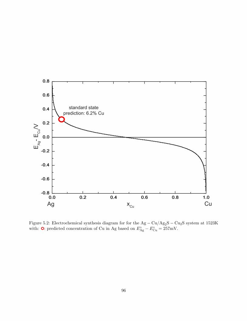
Ε Ag- Ε C
u/V
Ag CuxCu
standard stateprediction: 6.2% Cu
Figure 5.2: Electrochemical synthesis diagram for for the Ag− Cu/Ag2S− Cu2S system at 1523Kwith: : predicted concentration of Cu in Ag based on EAg − ECu = 257mV.
96
5.2 Background
The ability of molten sulfides to solubilize many different materials make traditional electro-
chemical activity measurements challenging. Metal references are frustrated by exchange interac-
tions and metallothermic reduction, which cause the reference to gradually change concentration
over the course of the experiment and drift electrochemical measurements. Attempts to use a Cu-
selective β”-Al2O3 membrane were unsuccessful due to exchange interactions between aluminum
and barium. The possibility of making a reference electrode inspired by aqueous capillary reference
electrodes was explored, but the supporting electrolyte reacted with the refractory materials used
to make the capillary, again causing a compositional drift.
Equilibration measurements have been successfully used in literature to determinine the activ-
ities of the CuS0.5 −MnS system, as well as the CuS0.5 −MnS− FeS system [16, 17]. In this type
of measurement, a metal is placed in contact with a solution of interest, and species are allowed
to exchange until equilibrium has been achieved. The activity of the electrolyte may be obtained
with the relation:
aAX = KaAaX (5.1)
where K is the equilibrium constant of the reaction A+X = AX.
In certain cases, the anionic species is difficult to measure and only the activities of the metal
are known. Without a sulfur-based reference electrode, it was impossible measure exactly how
much sulfur was being produced during equilibration. Additionally, no assumptions could be made
about whether sulfur was present in a gaseous or dissolved phase, in contrast to the studies in [16,
17]. Because of this, direct activity measurements were not possible, and an equilibrium synthesis
diagram was used in order to determine the decomposition potential difference of two electroactive
species as a function of their metallic concentration. This potential difference was converted to the
relative activities of the electrolyte species (see Chapter 3).
97

5.3 Activity Measurements
5.3.1 Experimental Methods
Barium sulfide (BaS, Alfa Aesar, 99.7% metals basis), lanthanum sulfide (La2S3, Strem Chem-
icals, 99.9% metals basis), copper sulfide (Cu2S, Strem Chemicals, 99.5% metals basis), and silver
sulfide (Ag2S, Alfa Aesar, 99.9% metals basis) were used to prepare the electrolyte. Based on the re-
sults of previous experiments in the BaS-La2S3-Cu2S system, the BaS-La2S3 supporting electrolyte
was fixed at 90wt% of the total electrolyte. The remaining 10% consisted of Cu2S-Ag2S.
It was observed that a homogenous sulfide melt could not be obtained if BaS, La2S3, Cu2S,
and Ag2S were mixed as powders in a crucible and melted together at high temperature. However,
BaS, La2S3, and Cu2S could be melted easily. Therefore, a two-step melting process was devised.
A 90% BaS-La2S3, 10% Cu2S mix was first melted together at 1523 K in an argon atmosphere (Ar,
Airgas, Ultra High Purity). The resulting sulfide was then crushed back into powder form in an
argon glovebox (Ar, Airgas, Ultra High Purity), and the necessary amount of Ag2S to reach the
desired final concentration was measured. Additional amounts of BaS-La2S3 were also added in
order to maintain the supporting electrolyte at 90%. This new mix was then melted a second time
in argon atmosphere.
For all melts, the sulfides were contained in a crucible machined from graphite (C, The Graphite
Store, Grade EC-16) and fitted with a graphite cap that fit tightly into the crucible in order to
limit possible sulfide volalization (Figure 5.3 a). This crucible was then loaded into an alumina
tube and placed into a vertical tube furnace (Lindberg/Blue MTM Mini-MiteTM). Inside the tube,
an alumina rod containing either a sheathed “Type R” or “Type C” thermocouple served as a stage
to both measure the temperature of the crucible as well a hold the crucible in the furnace hot zone.
The experimental setup is shown in Figure 5.4.
Pure silver (Ag, Alfa Aesar, 99.999% metals basis) was used as the metal for equilibration
experiments. Silver containing small quantities of oxygen is known to violently expel oxygen upon
solidification, and with it, small amounts of silver [18]. This phenomenon was observed to occur
in silver samples during sulfide equilibration, hindering efforts to fully analyze the metal post-
98

a)
b)
0.5cm
1cm
Figure 5.3: a) graphite crucible and cap used for sulfide melts and equilibration experiments b)sulfide sample and metal taken from crucible post-equilibration experiment.
99
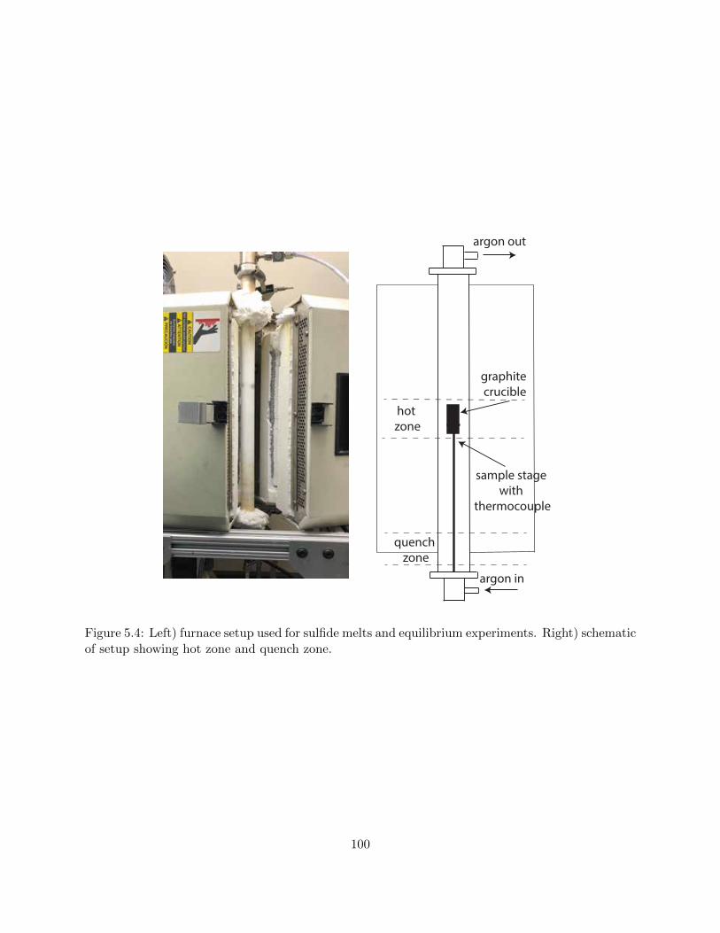
argon in
argon out
sample stage with
thermocouple
graphite crucible
hot zone
quench zone
Figure 5.4: Left) furnace setup used for sulfide melts and equilibrium experiments. Right) schematicof setup showing hot zone and quench zone.
100

equilibrium. Therefore, the silver was de-oxygenated prior to experimentation. Approximately
0.1 g of Ag was melted in an arc melter (Compact Arc Melter MAM-1, Edmund Buhler) under
Ar atmosphere in the presence of a zirconium oxygen getter (Zr, Alfa Aesar, 99.5% metals basis
(excluding Hf), Hf 3%).
The de-oxygenated silver was then combined with the pre-melted sulfide in a graphite crucible
and after evacuating and purging with Ar three times, was allowed to equilibrate at 1523K for 24
hours. At this time, the sample was lowered from the hot zone into the cooling zone (Figure 5.4).
As the cooling zone was near the Ar inlet, the flow of Ar was increased to allow for an even
more rapid cool. Figure 5.3 b shows an example of the metal and sulfide taken from the crucible
post-equilibration. Once fully cool, the metal was mounted in epoxy, polished, and examined
by scanning electron microscopy energy dispersive X-ray spectroscopy (SEM-EDS) to determine
the Cu-Ag ratio. The sulfide was analyzed by an inductively coupled plasma atomic emission
spectrometer (ICP-AES) in order to measure the change in content of Ba, La, S, Cu, and Ag.
5.3.2 Results
Upon examining the equilibrated metal, it was found that some exchange had taken place be-
tween Ag and Cu. Figure 5.5 shows the amounts of Cu measured in the Ag metal post-experiment.
Cu content varied from as low as 3 mol% to 21 mol%. Generally, as the concentration of Cu2S
increased along the Cu2S-Ag2S pseudobinary, the more Cu was found in the metal reference. How-
ever, near 40% Cu2S, there was a notable increase of Cu concentration in Ag metal.
The Ag-Cu equilibrium electrochemical synthesis diagram from Figure 5.2 was used to determine
the equilibrium difference in reduction potentials of Ag2S and Cu2S. This potential difference
was used to compute the relative activity aCu2S . Figure 5.6 shows the Wagner-Allanore activity
coefficient ρCu2S as a function of Cu2S concentration.
On the Cu2S-rich half of the Ag2S-Cu2S pseudobinary, ρCu2S ≈ 1. This indicates that Ag2S
and Cu2S are behaving ideally with respect to one another in the BaS-La2S3 supporting electrolyte.
Although the absolute activities of Ag2S and Cu2S are still unknown, this result means that both
species interact with the supporting electrolyte in a similar way: if the absolute activity of Ag2S is
101

Cu2SAg2S xCu S2
x Cu
x Cu+
x Ag
Figure 5.5: Measured Cu content in Ag metal after equilibration with molten BaS-La2S3-Cu2S-Ag2Sat 1523K for 24 hours.
102
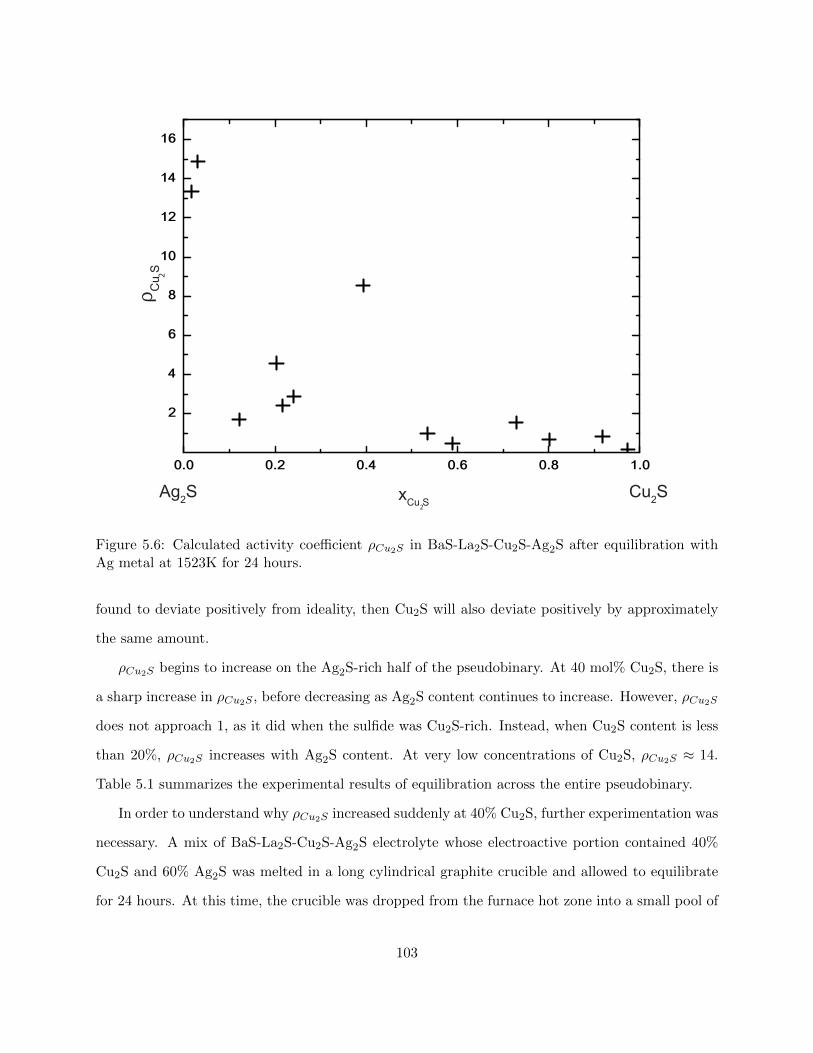
Cu2SAg2S xCu S2
Cu
S 2
Figure 5.6: Calculated activity coefficient ρCu2S in BaS-La2S-Cu2S-Ag2S after equilibration withAg metal at 1523K for 24 hours.
found to deviate positively from ideality, then Cu2S will also deviate positively by approximately
the same amount.
ρCu2S begins to increase on the Ag2S-rich half of the pseudobinary. At 40 mol% Cu2S, there is
a sharp increase in ρCu2S , before decreasing as Ag2S content continues to increase. However, ρCu2S
does not approach 1, as it did when the sulfide was Cu2S-rich. Instead, when Cu2S content is less
than 20%, ρCu2S increases with Ag2S content. At very low concentrations of Cu2S, ρCu2S ≈ 14.
Table 5.1 summarizes the experimental results of equilibration across the entire pseudobinary.
In order to understand why ρCu2S increased suddenly at 40% Cu2S, further experimentation was
necessary. A mix of BaS-La2S-Cu2S-Ag2S electrolyte whose electroactive portion contained 40%
Cu2S and 60% Ag2S was melted in a long cylindrical graphite crucible and allowed to equilibrate
for 24 hours. At this time, the crucible was dropped from the furnace hot zone into a small pool of
103

Table 5.1: Cu content in Ag after equilibration and measured ρCu2S .
Cu2S Cu ρCu2S(mol%) (mol%)
1.7 2.9 13.4
3.1 4.2 14.9
12.1 2.9 1.7
20.3 6.7 4.6
21.7 5.0 2.4
24.1 5.9 2.9
39.3 15.3 8.53
53.4 6.6 0.9
58.9 5.0 0.5
72.9 13.1 1.5
80.1 10.7 0.7
91.8 20.6 0.9
97.3 17.4 0.2
liquid gallium for a more aggressive quench. The sample was then removed from the crucible and
sectioned lengthwise before being analyzed by SEM-EDS.
Upon solidification, two main phases were observed to form: a primary phase, and a secondary
intergrain phase (Figure 5.7). Examination of each phase under SEM-EDS showed a similar segre-
gation of Ag and Cu between the two phases as that observed when looking at the variation of Cu
and Ag with crucible position. The Ag-Cu content in the first phase to form, the primary phase,
contained 65% Ag on average, while the secondary phase contained only 52%. In certain areas
of the crucible, a tertiary phase observed to occasionally form. There was no significant Cu-Ag
segregation observed in this phase.
Figures 5.8 and 5.9 show the variation in Cu and Ag content in the electrolyte from the bottom
of the crucible to the top. Figure 5.8 shows that there was a higher concentration of Ag sulfides
at the bottom of the crucible, while the electrolyte near the top was enriched in Cu sulfide. The
average Ag-Cu content in the bottom half of the crucible was 66 mol% Ag, while the average Ag-Cu
content in the top half of the crucible was only 57% Ag. The average overall Ag-Cu content was
62% Ag.
104
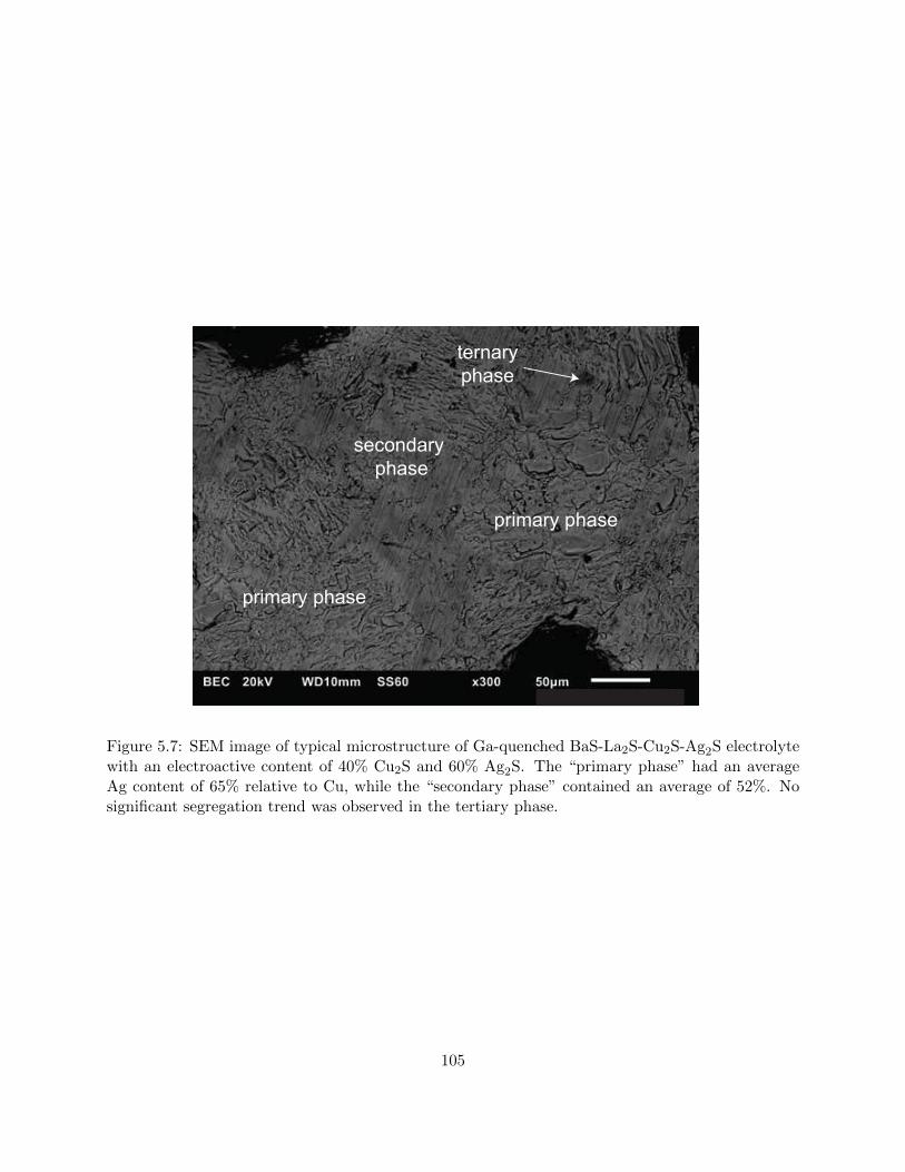
primary phase
secondary phase
ternaryphase
primary phase
Figure 5.7: SEM image of typical microstructure of Ga-quenched BaS-La2S-Cu2S-Ag2S electrolytewith an electroactive content of 40% Cu2S and 60% Ag2S. The “primary phase” had an averageAg content of 65% relative to Cu, while the “secondary phase” contained an average of 52%. Nosignificant segregation trend was observed in the tertiary phase.
105
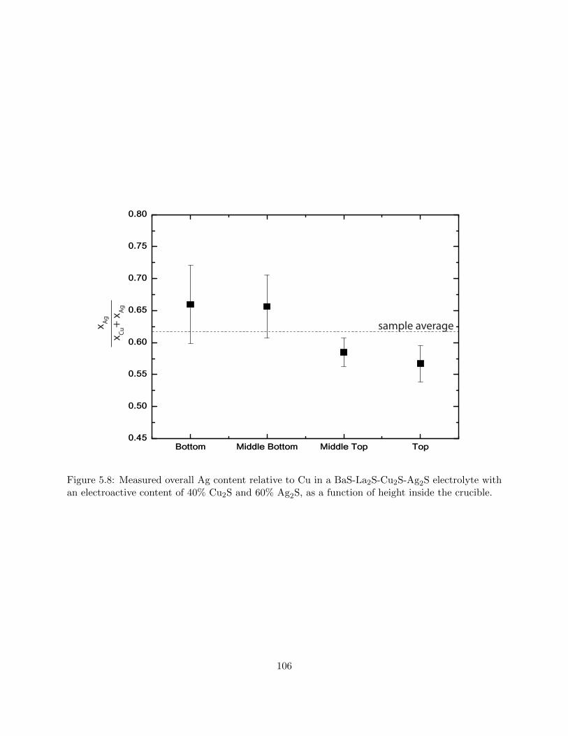
sample average
x Cu+
x Ag
x Ag
Figure 5.8: Measured overall Ag content relative to Cu in a BaS-La2S-Cu2S-Ag2S electrolyte withan electroactive content of 40% Cu2S and 60% Ag2S, as a function of height inside the crucible.
106
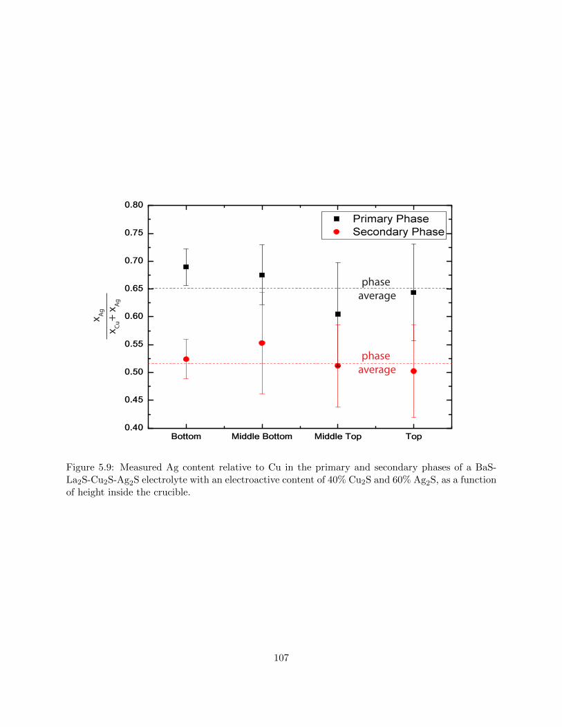
phase average
phase average
x Ag
x Cu+
x Ag
Figure 5.9: Measured Ag content relative to Cu in the primary and secondary phases of a BaS-La2S-Cu2S-Ag2S electrolyte with an electroactive content of 40% Cu2S and 60% Ag2S, as a functionof height inside the crucible.
107

5.4 Discussion
5.4.1 Equilibration Experiments
Despite a 257mV decomposition potential difference between Ag2S and Cu2S, significant ex-
change between Cu2S and Ag was observed to occur, forming Cu and Ag2S. On the Cu2S-rich side,
ρCu2S ≈ 1 and observed Cu content in the metal was consistent with ideal-solution predictions
from the electrochemical synthesis diagrams. When Ag2S and Cu2S behave ideally relative to one
another, they are interacting with the supporting electrolyte in a similar way and electrolyte ther-
modynamics do not contribute to co-deposition. This result indicates that, when the electrolyte is
rich in Cu2S, the observed alloying of Ag and Cu comes from the thermodynamic drive for mixing
the two metals.
In contrast, when the electrolyte contains more Ag2S, the electrolyte begins to deviate from
ideality. More Cu is alloyed into the Ag than would be predicted from an EESD using an ideal-
solution assumption. The activity coefficient ρCu2S was found to deviate positively from ideality in
this concentration range. Additionally, there was a sharp increase in the activity coefficient when
the Ag2S-Cu2S fraction was equal to 0.4 Cu2S. This corresponded to a larger amount of Cu alloying
in the Ag metal.
ρCu2S > 1 signifies that Cu2S has a higher activity coefficient in the electrolyte than Ag2S.
Relative to Ag2S, Cu2S has a more positive deviation from ideality. A positive deviation from
ideality signifies an increase in Gibbs energy upon mixing, or a tendency for phase separation,
while a negative deviation from ideality signifies an increased energetic drive for mixing. Therefore,
ρCu2S > 1 indicates that the BaS-La2S3 electrolyte favors energetic bonds with Ag2S over Cu2S.
Such behavior is supported by the observation a BaS-La2S3-Ag2S electrolyte required a higher
temperature to melt successfully. Additionally, the BaS-La2S3-Ag2S electrolyte was very dense,
with the Ag metal reference floating to the top of the sulfide. Strong bonding between the sulfide
species could be one reason for the increase in density.
The sudden increase in ρCu2S at 40% Cu2S suggests similar preference for bonds between Ag2S
and the supporting BaS-La2S3 electrolyte at this composition. One possible explanation for this
108
phenomenon could be the formation of a compound near this composition. This would result in
short-range ordering between Ag2S and the BaS-La2S3 supporting electrolyte in the liquid after this
compound melted. Since ρCu2S is a relative value, however, it only signifies that there is a strong
preference for the supporting electrolyte to interact with Ag2S instead of Cu2S. Therefore, while
short-range ordering between Ag2S and the supporting electrolyte is possible, it is also possible
that there is phase separation between Cu2S and the supporting electrolyte.
5.4.2 Gallium Quench Experiment
During the gallium quenching experiment, it was found that there was an increased concen-
tration of Ag2S towards the bottom of the crucible, while the top of the crucible was richer in
Cu2S (Figure 5.8). This is in keeping with the observation that Ag2S-rich electrolytes were more
dense than their Cu2S counterparts. Furthermore, while the overall concentration of the sulfide
remained near the 40% Cu2S-60% Ag2S concentration, the bottom half of the crucible differed by
almost 10mol% from the top half. This result points to evidence of possible phase separation be-
tween Cu2S-rich electrolyte and Ag2S-rich electrolyte in the liquid phase, with the denser Ag2S-rich
liquid sinking to the bottom of the crucible.
Additionally, the first two phases to nucleate upon solidification also displayed similar segrega-
tion of Cu2S and Ag2S (Figure 5.9). The primary phase was Ag2S-rich, with an average composition
near that of the average composition of the Ag2S-rich bottom half of the crucible. That the Ag2S-
rich phase was the first to nucleate supports the hypothesis that there is favorable bonding between
Ag2S and the supporting electrolyte, and is consistent with observations of higher melting points
for Ag2S-rich electrolytes. The second phase to form contained higher amounts of Cu2S, similar to
the top half of the crucible.
Both micro- and macro- scale segregation of Ag2S and Cu2S was observed, with there being an
overall tendency towards Ag2S-enrichment at the bottom of the crucible, as well as the nucleation
of a Ag2S-rich phase and a Cu2S-rich phase upon solidification. These results suggest there are
very different energetic interactions between Ag2S and the supporting electrolyte, and between
Cu2S and the supporting electrolyte. These results are also consistent with increase in ρCu2S at
109

this concentration.
Although ρCu2S is a relative activity, it retains important information about electrolyte inter-
actions. Deviations from ideality that suggest certain phase phenomena, such as phase separation
or compound formation, are still measured. In the case of a BaS-La2S-Cu2S-Ag2S electrolyte,
these phenomena could be confirmed by microscopy, which revealed that Ag2S and Cu2S interact
differently with BaS-La2S.
By examining the results of the equilibrium experiments alongside the activity calculations and
its consequences on the electrolyte’s phase relations, it is possible to gain new insights on the BaS-
La2S-Cu2S-Ag2S system. Because of molten sulfides’ high degree of reactivity, it would be difficult
to obtain this information through conventional, direct activity measurements. However, relative
activity measurements are possible because the only condition on reactivity is that equilibrium
is reached: any degree of cross-reaction between the electrolyte and the reference can be directly
correlated to thermodynamic properties by using an equilibrium electrochemical synthesis diagram.
In the case of Cu2S-Ag2S, it could be seen that metal interactions (the drive for Cu and Ag to alloy)
dominate the reaction on the Cu2S-rich side of the pseudobinary, while electrolyte interactions (the
preference for the supporting electrolyte to mix with Ag2S over Cu2S) become more significant on
the Ag2S-rich side. From this, optimal conditions for electrolyte composition during electrolysis can
be determined. While the drive for Cu to alloy in a Ag cathode will always be present, operating
electrolysis on the Cu2S-rich prevents further complications due to electrolyte interactions. On the
Cu2S-rich side of the pseudobinary, there are no interactions in the electrolyte that favor electrolysis
of either Ag or Cu. On the Ag2S-rich side, however, unfavorable interactions between Ag2S and
BaS-La2S will push the reaction towards Cu electrolysis by raising the activity of Cu2S.
When considering molten sulfide electrolysis as a possible pathway for electronic waste recycling,
therefore, it is suggested that the electrolyte contains at least as much Cu2S as Ag2S in order to
avoid unwanted interactions between Ag2S and the supporting electrolyte. An experimental study
of Ag-Cu electrolysis in molten sulfides will be presented in Chapter 6.
110
5.5 Summary
Activity measurements in high temperature liquid electrolytes are challenging due to the pos-
sibility of reactivity with the references necessary for accurate measurement. Molten sulfides are
one such case. However, through measuring relative activity, it is possible to obtain useful insights
about the thermodynamics of a system. As seen in the study of BaS-La2S-Cu2S-Ag2S, activity
measurements in the Wagner-Allanore reference state provided useful thermodynamic information
about the electrolyte, which will be used in Chapter 6 to design electrochemical experiments.
Activity measurements of the system indicated a difference in mixing behavior between BaS-
La2S-Cu2S and BaS-La2S-Ag2S. This was later confirmed by quenching and microscopy, which
revealed phase separation between Cu2S and Ag2S containing phases. It was observed that when the
electrolyte contains more Cu2S, Cu2S and Ag2S behave ideally with respect to one another. Ideal
behavior minimizes unfavorable electrolyte interactions that can favor Cu deposition. Therefore,
if a pure Ag product is desired, the electrolyte should contain sufficient Cu2S to reduce risk of
codeposition.
111
Bibliography
[1] Mark D. Barton. “The Ag-Au-S System”. In: Economic Geology 75 (1980), pp. 303–316. issn:
0361-0128. doi: 10.2113/gsecongeo.75.2.303.
[2] G.A. Pal’yanova and N.E. Savva. “Some Sulfides of Gold and Silver: Composition, Mineral
mineral Assemblage, and Conditions of Formation”. In: Theoretical Foundations of Chemical
Engineering 42.5 (2008), pp. 749–761. doi: 10.1134/S0040579508050485.
[3] Galina Palyanova, Nick Karmanov, and Natalie Savva. “Sulfidation of native gold”. In: Amer-
ican Mineralogist 99.5-6 (2014), pp. 1095–1103. doi: 10.2138/am.2014.4677.
[4] J. D. Scott. “Electrometallurgy of copper refinery anode slimes”. In: Metallurgical Transac-
tions B 21.4 (Aug. 1990), pp. 629–635. issn: 0360-2141. doi: 10.1007/BF02654241. url:
http://link.springer.com/10.1007/BF02654241.
[5] C Segawa and T Kusakabe. “Current Operations in SMM’s Slime Treatment”. In: TMS
Extraction and Processing Division. Anaheim, Ca, 1996. url: http://www.isasmelt.com/
EN/Publications/TechnicalPapersBBOC/SMM’s%20Slime%20Treatment.pdf.
[6] T Chen and J E Dutrizac. “Mineralogical overview of the behavior of gold in conventional
copper electrorefinery anode slimes processing circuits”. In: J E Minerals & Metallurgical
Processing Aug 25.3 (2008), pp. 156–164.
[7] Ailiang Chen et al. “Recovery of Silver and Gold from Copper Anode Slimes”. In: JOM
Journal of the Minerals, Metals and Materials Society 67.2 (2015), pp. 493–502. doi: 10.
1007/s11837-014-1114-9.
112

[8] S.A. Mastyugin and S.S. Naboichenko. “Processing of Copper-Electrolyte Slimes: Evolution
of Technology”. In: Russian Journal of Non-Ferrous Metals 53.5 (2012), pp. 367–374. doi:
10.3103/S1067821212050070.
[9] J Hait, R K Jana, and S K Sanyal. “Processing of copper electrorefining anode slime:
a review”. In: Trans. Inst. Min. Metall. C. 118.4 (2009), pp. 240–252. doi: 10 . 1179 /
174328509X431463.
[10] K G Fisher. “Refining of Gold At the Rand Refinery”. In: Extractive Metallurgy of Gold in
South Africa. Ed. by G.G. Stanley. Johannesburg: South African Institution of Mining and
Metallurgy, 1987. Chap. 10, pp. 615–653. isbn: 978-1468484274.
[11] Jirang Cui and Lifeng Zhang. “Metallurgical recovery of metals from electronic waste: A
review”. In: Journal of Hazardous Materials 158.2-3 (2008), pp. 228–256. issn: 03043894.
doi: 10.1016/j.jhazmat.2008.02.001.
[12] C. W. Bale et al. “FactSage thermochemical software and databases, 2010-2016”. In: Calphad
54 (Sept. 2016), pp. 35–53. issn: 03645916. doi: https://doi.org/10.1016/j.calphad.
2016.05.002.
[13] Caspar Stinn et al. “Experimentally Determined Phase Diagram for the Barium Sulfide-
Copper(I) Sulfide System Above 873 K (600 °C)”. In: Metallurgical and Materials Trans-
actions B 48.6 (2017), pp. 2922–2929. doi: 10.1007/s11663-017-1107-5. url: https:
//link.springer.com/content/pdf/10.1007/s11663-017-1107-5.pdf.
[14] Charles Cooper Rinzler. “Quantitatively Connecting the Thermodynamic and Electronic
Properties of Molten Systems”. PhD. Massachusetts Institute of Technology, 2017.
[15] Sulata K. Sahu, Brian Chmielowiec, and Antoine Allanore. “Electrolytic Extraction of Cop-
per, Molybdenum and Rhenium from Molten Sulfide Electrolyte”. In: Electrochimica Acta
243 (2017), pp. 382–389. issn: 00134686. doi: 10.1016/j.electacta.2017.04.071.
[16] Yun Lei et al. “Thermodynamic properties of the MnS-CuS0.5 binary system”. In: ISIJ
International 52 (2012), pp. 1206–1210. doi: 10.2355/isijinternational.52.1206. url:
113

https://www.jstage.jst.go.jp/article/isijinternational/52/7/52%7B%5C_
%7D1206/%7B%5C_%7Dpdf.
[17] Yun Lei et al. “Thermodynamic properties of the FeS-MnS-CuS0.5 ternary system at 1473 K”.
In: ISIJ International 53 (2013), pp. 966–972. doi: 10.2355/isijinternational.53.966.
url: https://www.jstage.jst.go.jp/article/isijinternational/53/6/53%7B%5C_
%7D966/%7B%5C_%7Dpdf.
[18] Manuel Eissler. The Metallurgy of Silver: A Practical Treatise on the Amalgamation, Roasting
and Lixiviation of Silver Ores Including the Assaying, Melting and Refining of Silver Bullion.
3rd. London: Crosby, Lockwood, and son, 1896, p. 336.
114
Chapter 6
Electrochemistry in Molten Sulfides
The aim of this thesis work is to develop a method for characterizing novel electrolytes in order
to facilitate development of new electrochemical processes. The derivations put forth in Chapter 3
allow the experimentalist to easily measure the activity of novel electrolytes, enabling them to
access previously unknown thermodynamic properties. Although the activity is only measured
relative to another species in the electrolyte, much of the thermodynamic information important
to determine the electrolyte’s performance is retained, as was demonstrated in Chapters 4 and 5.
In this chapter, the applications of the model are tested further. Activity measurements in the
BaS-La2S-Cu2S-Ag2S system (Chapter 5) are used to design electrochemical experiments to test
the selectivity of Ag deposition over Cu deposition. An additional system relevant to primary metal
production, Cu electrolysis from CuFeS2, will also be examined in light of the insights gained from
activity measurements in the BaS-La2S-Cu2S-FeS system. Predictions of cathode composition will
be compared to experimental electrolysis results and used to evaluate the efficacy of the proposed
model.
6.1 Ag-Cu Separation
The first experimental system studied is Ag-Cu deposition from a molten sulfide electrolyte. In
order to use molten sulfides as an effective means of recycling electronic waste, it is necessary to be
115

able to selectively deposit first Ag, and then Cu from the mutually soluble electrolyte. Both cathode
products should be relatively pure to minimize the need for further refinement and downstream
processing [1–3].
Based on the results of Chapter 5, a molten sulfide electrolyte containing at least as much
Cu2S as Ag2S should be used. In this concentration range, there were no measured electrolyte
interactions that would favor Cu deposition over Ag deposition, and the energetic drive for Cu to
alloy with Ag will be the only factor contributing to significant Cu production.
An electrolyte composition consisting of 90wt% BaS-La2S3 supporting electrolyte, and 10wt%
Cu2S-Ag2S was chosen based on success in previous experimental studies [4]. The Cu2S-Ag2S
portion of the electrolyte consisted of 5mol% Ag2S and 5mol% Cu2S. In this concentration range,
Cu2S as Ag2S behave ideally with respect to one another. Additionally, as the goal is to reduce
Ag2S to Ag metal first, depletion of Ag2S and the resulting concentration shift during electrolysis
will only ensure that the electrolyte composition remains favorable. As Ag2S is depleted, the
electrolyte will remain on the Cu2S-rich side of the pseudobinary. In contrast, if one were to start
with a high concentration of Ag2S instead, not only would there be an energetic drive on the
electrolyte side to deposit Cu, but as Ag2S is depleted, the electrolyte risks nearing the 60%Ag2S-
40%Cu2S concentration. Thermodynamic measurements taken at this composition indicate a large,
positive, energy of mixing for Cu2S with the supporting electrolyte, which would further favor
Cu deposition. Additionally, the concentration gradients noticed at this composition as a result
of density differences between BaS-La2S3-Cu2S and BaS-La2S3-Ag2S could have further negative
effects on the electrochemical cell: depending on the cell arrangement, there could be a different
electrolyte composition between the anode and the cathode, even without mass transfer effects.
6.1.1 Experimental Methods
A two-electrode setup was used for the electrolysis experiments, with a liquid metal cathode
consisting of either Ag or a Ag-Cu alloy (Ag, Alfa Aesar, 99.9985% metals basis), (Cu, Alfa Aesar,
99.999% metals basis), and a graphite anode (C, Alfa Aesar, 99.9995% metals basis). 5g of a BaS-
La2S3-Cu2S-Ag2S electrolyte was prepared using both the materials and the two-step pre-melting
116
process described in Chapter 5. The Ag-Cu alloy was prepared by melting approximately 5g of
metal inside an arc melter (Compact Arc Melter MAM-1, Edmund Buhler) under Ar atmosphere
in the presence of a zirconium oxygen getter (Zr, Alfa Aesar, 99.5% metals basis (excluding Hf),
Hf 3%). When an alloy was prepared, it was melted inside the arc melter 3 times, flipping the
solidified metal piece in between melts in order to ensure homogeneity.
Both the metal and sulfide were then loaded into a graphite crucible that was sheathed on
the sides by an alumina tube. A molybdenum wire (Mo, Ed Fagan Inc., ASTM B387 Type 361,
99.95% pure) was threaded into the bottom of the graphite crucible and secured with graphite
paste (PELCO High Temperature Carbon Paste, Ted Pella, Inc.) to provide electrical contact to
the cathode. This Mo wire was protected by an alumina tube that provided mechanical support to
the setup and also contained a type C thermocouple used to monitor the cell’s temperature.
A second Mo wire was threaded into the graphite anode, and after being secured with graphite
paste, was positioned just above the electrolyte, and the entire setup was loaded into a vertical
tube furnace (Lindberg/Blue MTM Mini-MiteTM) and heated to 1523 K after being evacuated and
purged with argon (Ar, Airgas, Ultra High Purity) three times.
Once the electrolyte was fully molten, the anode was lowered into the melt and galvanostatic
electrolysis was run immediately to ensure any compositional changes in the metal were a result of
electrochemistry, not equilibrium exchange. At the end of the experiment, the electrochemical cell
was immediately quenched by lowering the crucible out of the hot zone, the center of the furnace
where the heat is concentrated, to the bottom of the furnace tube where cold Ar flows in. As in the
quench methodology described in Chapter 5, the flow of Ar into the tube was increased in order to
facilitate a more rapid quench.
Electrolysis experiments were run using a Gamry Potentiostat/Galvanostat (Gamry Instru-
ments, Reference 3000), and temperature was monitored using an Omega data aquisition system
(Omega Engineering, Model QMB-DAQ-55). All electrolysis experiments were run at a low cathode
current density to minimize kinetic effects: 12mA/cm2. A schematic of the electrochemical cell
used for all experiments is shown in Figure 6.1.
Post-experiment, the metal cathode was separated from the sulfide electrolyte and was mounted
117

graphite crucible
aluminasheath
graphite anode
BaS-La2S3-Cu2S-Ag2S electrolyte
silver-copper alloy cathode
1cm
Figure 6.1: Left) schematic of electrochemical cell used for Cu-Ag separation experiments. Right)cathode and electrolyte after electrolysis experiment
118

in epoxy, polished, and examined using a scanning electron microscope’s energy dispersive X-ray
spectroscopy (SEM-EDS) to measure compositional changes from the initial Cu-Ag alloy.
6.1.2 Results
Figure 6.2 shows the total cell potential measured during a series of 12mA/cm2 chronopoten-
tiometry experiments in a BaS-La2S3-Cu2S-Ag2S electrolyte. The electroactive (non-supporting)
portion of this electrolyte contained 50% Cu2S and 50% Ag2S, and the starting cathode compo-
sition contained varying amounts of Cu, from 0mol% to 10mol%. The measured cell potential
gradually increased in magnitude over the time of the experiment, rather than stabilizing at one
single potential. The electrochemical signals displayed regular oscillations, likely a result of heating
element and thermocouple interference, but were overall very stable throughout electrolysis.
Table 6.1 shows the change in cathode composition during electrolysis, and Figure 6.3 compares
the measured composition change to the equilibrium Cu content for the chosen electrolyte. It can
be seen that when starting with a cathode of pure Ag, Cu is deposited on the cathode. When
electrolysis was only run for 1 hour, the cathode was found to contain 0.8mol%Cu. However, when
electrolysis was run for a longer amount of time, 3.5 hours, further enrichment of the cathode was
observed: the final measured composition was 1.14mol%Cu.
If the starting cathode composition contained Cu, Ag was deposited on the cathode instead. In
these cases, the shift in cathode composition appeared to be proportional to how far the composition
was from equilibrium. A large compositional shift of 2.7mol% was observed to take place when the
starting alloy contained 10mol% Cu, while smaller shifts of 0.7mol% and 0.5mol% were found when
the starting alloy contained 6mol% and 4.5mol%, respectively.
6.1.3 Discussion
It can be seen that when starting with a cathode of pure Ag, there is a strong drive for Cu
deposition in order to reach this equilibrium composition. This drive causes the reduction of Cu
over Ag, even though the measured difference in reduction potential between Cu2S and Ag2S for
this electrolyte composition should be 265mV. In order to affirm that Cu deposition was an elec-
119
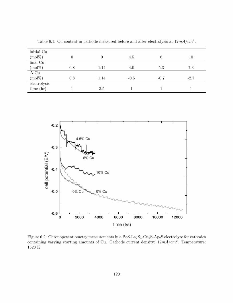
Table 6.1: Cu content in cathode measured before and after electrolysis at 12mA/cm2.
initial Cu(mol%) 0 0 4.5 6 10
final Cu(mol%) 0.8 1.14 4.0 5.3 7.3
∆ Cu(mol%) 0.8 1.14 -0.5 -0.7 -2.7
electrolysistime (hr) 1 3.5 1 1 1
cell
pote
ntia
l (E/
V)
time (t/s)
10% Cu
6% Cu
4.5% Cu
0% Cu 0% Cu
Figure 6.2: Chronopotentiometry measurements in a BaS-La2S3-Cu2S-Ag2S electrolyte for cathodescontaining varying starting amounts of Cu. Cathode current density: 12mA/cm2. Temperature:1523 K.
120
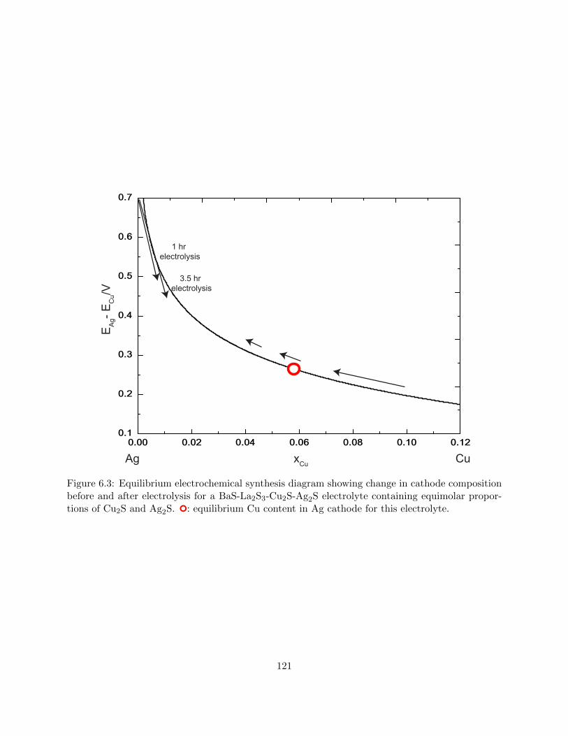
Ag CuxCu
Ε Ag- Ε C
u/V 3.5 hr
electrolysis
1 hr electrolysis
Figure 6.3: Equilibrium electrochemical synthesis diagram showing change in cathode compositionbefore and after electrolysis for a BaS-La2S3-Cu2S-Ag2S electrolyte containing equimolar propor-tions of Cu2S and Ag2S. : equilibrium Cu content in Ag cathode for this electrolyte.
121

trochemical phenomena, the dependence of concentration shift on electrolysis time was measured.
It was found that the longer an experiment was run, the more Cu was alloyed into the cathode
(Figure 6.3).
Conversely, when starting with a cathode enriched in Cu, there is a strong drive for Ag deposi-
tion. When the starting composition contains 10mol%Cu, enough Ag is deposited during electrol-
ysis to shift the composition by 2.7%. Such a compositional shift is not possible by electrochemical
means alone, even if the cell were operating at 100% Faradaic efficiency. This indicates that Ag
was also cuprothermically reduced by the following reaction:
Ag2S + Cu→ Cu2S + Ag (6.1)
When the cathode contains 10mol% Cu, both the electrolyte and the cathode favor Ag depo-
sition. With an equilibrium concentration of 5.8% Cu, increasing Ag content through deposition
will lower the Cu concentration of the cathode and thus lower its Gibbs energy. In addition, the
electrolyte also favors Ag deposition by a 265mV potential difference. These twin driving forces
contributed to the significant cathode enrichment in Ag over the course of the experiment.
When the cathode contained moderate amounts of Cu, such as 4.5% or 6%, the cathode was
closer to its equilibrium composition and there was less of a drive for Ag deposition as a result.
The cathode was observed to increase in Ag content through both experiments.
When the cathode contained 4.5% Cu, one might expect that Cu be deposited on the cathode
instead of Ag in order to reach the equilibrium concentration. However, Ag was deposited in-
stead. There are several reasons why this may occur. First, it has been shown that the kinetic and
transport effects at play during electrolysis cannot be neglected entirely when using an equilibrium
electrochemical synthesis diagram to analyze electrochemical data (see Chapter 4). It is possible
that local concentration variations in the vicinity of the cathode caused the equilibrium concentra-
tion to shift, favoring Ag deposition instead. Given that the cell design was vertical, with the liquid
cathode at the bottom of the cell, and that BaS-La2S3-Cu2S and BaS-La2S3-Ag2S were found to
have different densities, such a concentration shift is certainly possible. Finally, in order to allow for
122
the anode to be lowered into the melt right at the start of electrolysis, the electrochemical cell was
open at the top. The absence of a cap may have allowed for certain elements to volatilize during
the experiment, which could shift the electrolyte concentration and in turn effect the equilibrium
Cu concentration in the cathode.
Despite these possible sources of error, the value of using the above approach to study electrolysis
can be clearly seen in Figure 6.3. The role that cathode chemistry plays in co-deposition is evident
from the difference in the amount of compositional shift, which varied depending on how far the
starting composition was from equilibrium. Additionally, by pre-screening the electrolyte with
equilibrium experiments, it was possible to gain an understanding of the electrolyte behavior, and
use this to select an appropriate concentration to run further experiments.
6.2 Fe-Cu Separation
The second molten sulfide electrochemical system considered is Fe-Cu extraction. Sufficient
separation of Fe and Cu in a molten sulfide electrolyte is essential to successful development of a
new pathway towards Cu deposition: direct electrolysis of copper-bearing sulfide ores to copper
metal [4, 5].
Chalcopyrite is one common Cu-bearing sulfide ore used in Cu production today. This mineral,
CuFeS2, contains equimolar amounts of Cu and Fe. In contrast to the oxide series, for the standard
state electrochemical series for sulfides, Fe is the more noble species (Figure 5.1). This means
that Fe must be successfully removed from the CuFeS2 before Cu can be extracted. However, the
decomposition potential difference between Cu and Fe is only 54mV at 1573K. This suggests that
separation of Cu and Fe through molten sulfide electrochemistry will be very challenging.
Analysis of the Cu-Fe system with an equilibrium electrochemical synthesis diagram, however,
indicates that electrochemical separation may be possible. At 1573 K, Cu and Fe phase separate
to form an Fe-rich solid and a Cu-rich liquid (Figure 6.4). If 17mol% (≈ 4.22wt%) carbon is added
to an iron cathode in order to depress the melting point, the region of phase separation widens. A
solution of copper and cast iron has a large positive energy of mixing, due to repulsive interactions
123

0 0.2 0.4 0.6 0.8 1273
473
673
873
1073
1273
1473
1673
1873
2073
Fe CuxCu
T/K
liquid
liquid + fcc
fcc(Fe) + fcc(Cu)
bcc(Fe) + fcc(Cu)
Figure 6.4: Fe-Cu phase diagram.
between Cu and both C and Fe. The effect of this thermodynamic can be seen in Figure 6.5. If the
electrolyte behaves ideally, the equilibrium cathode composition would be 2mol% Cu, less than that
predicted for Cu-Ag extraction, despite the significantly higher decomposition potential difference.
With encouraging preliminary model results indicating that Fe and Cu separation through
molten sulfide electrolysis is possible, it was necessary to confirm these predictions with experimen-
tation. Equilibrium experiments (as in Chapter 5) were run in order to measure the relative activity
of FeS and Cu2S in a BaS-La2S3 electrolyte. These results were then compared with electrolysis
experiments aimed at selectively depositing Fe from a molten sulfide electrolyte.
6.2.1 Experimental Methods
Graphite rods were dissolved into high purity electrolytic iron (Fe, Tophet Corporation) in an
induction melter to produce cast iron with minimal contaminants. Pieces of this cast iron were
124

0 0.2 0.4 0.6 0.8 1273
473
673
873
1073
1273
1473
1673
1873
2073
Fe + C CuxCu
T/K
liquid 1 + liquid 2 liquid 1 + liquid 2 + C
fcc + liquid + C
fcc 1 + fcc 2 + C
bcc + fcc + C
eesd temperature
liquid
1
liquid 2 + C
Fe + C CuxCu
Ε Fe- Ε C
u/V
Figure 6.5: a) Fe-Cu-C phase diagram when xCxF e+xC
= 0.17. b) equilibrium electrochemical syn-thesis diagram for the Fe − Cu − C/FeS − Cu2S system at 1573K. At this temperature, cast ironand Cu phase separate to form two different liquid solutions and solid C. : predicted Cu contentin cast iron (2 mol%), assuming ideal behavior in the electrolyte.
125
melted in an arc melter (Compact Arc Melter MAM-1, Edmund Buhler) under Ar atmosphere in
the presence of a zirconium oxygen getter (Zr, Alfa Aesar, 99.5% metals basis (excluding Hf), Hf
3%). LECO analysis of the cast iron found it to contain 19mol%C (≈ 5wt%).
Barium sulfide (BaS, Alfa Aesar, 99.7% metals basis), lanthanum sulfide (La2S3, Strem Chem-
icals, 99.9% metals basis), copper sulfide (Cu2S, Strem Chemicals, 99.5% metals basis), and iron
sulfide (FeS, Strem Chemicals, 99.9% metals basis) were used to prepare the electrolyte, which
contained 90wt% BaS-La2S3 and 5wt% each of FeS and Cu2S. These powders were mixed in an
argon glove box (Ar, Airgas, Ultra High Purity), and pre-melted in a graphite crucible. The melted
sulfide was then ground back into powder in the glove box before being added to an alumina cru-
cible (Al2O3, Advalue Technology) along with the cast iron. A piece of alumina was placed atop
the crucible as a loose-fitting cap to minimize volatilization, and the entire setup was loaded into
a vertical tube furnace (Lindberg/Blue MTM Mini-MiteTM). The crucible was supported by an
alumina stage containing an alumina-sheathed “Type R” thermocouple. With the exception of the
use of an alumina crucible in place of a graphite one, the equilibration setup was identical to the
one shown in Figure 5.4.
Galvanostatic electrolysis experiments were performed by colleagues in the Allanore Group and
full detail of the experimental setup will be given in an upcoming publication detailing the group’s
efforts to produce Cu from chalcopyrite by molten sulfide electrolysis. Similar to the Cu2S-Ag2S
electrolysis experiments, a pool of molten metal (C-saturated Fe) served as the cathode. Graphite
was used as the anode, and the cell setup was vertical, with the liquid cathode at the bottom and
C anode at the top. Post experiment, the composition of the cathode and sulfide were analyzed
with ICP-AES and LECO.
6.2.2 Results
After equilibration, the cast iron was found to contain 0.58mol% Cu. The electrolyte concen-
tration had shifted as well during the course of the experiment. ICP-AES analysis revealed that
the FeS-Cu2S portion of the sulfide contained approximately 76mol% FeS and 24mol% Cu2S.
These results give a value of ρCu2S = 0.46. This indicates that FeS and Cu2S do not behave
126
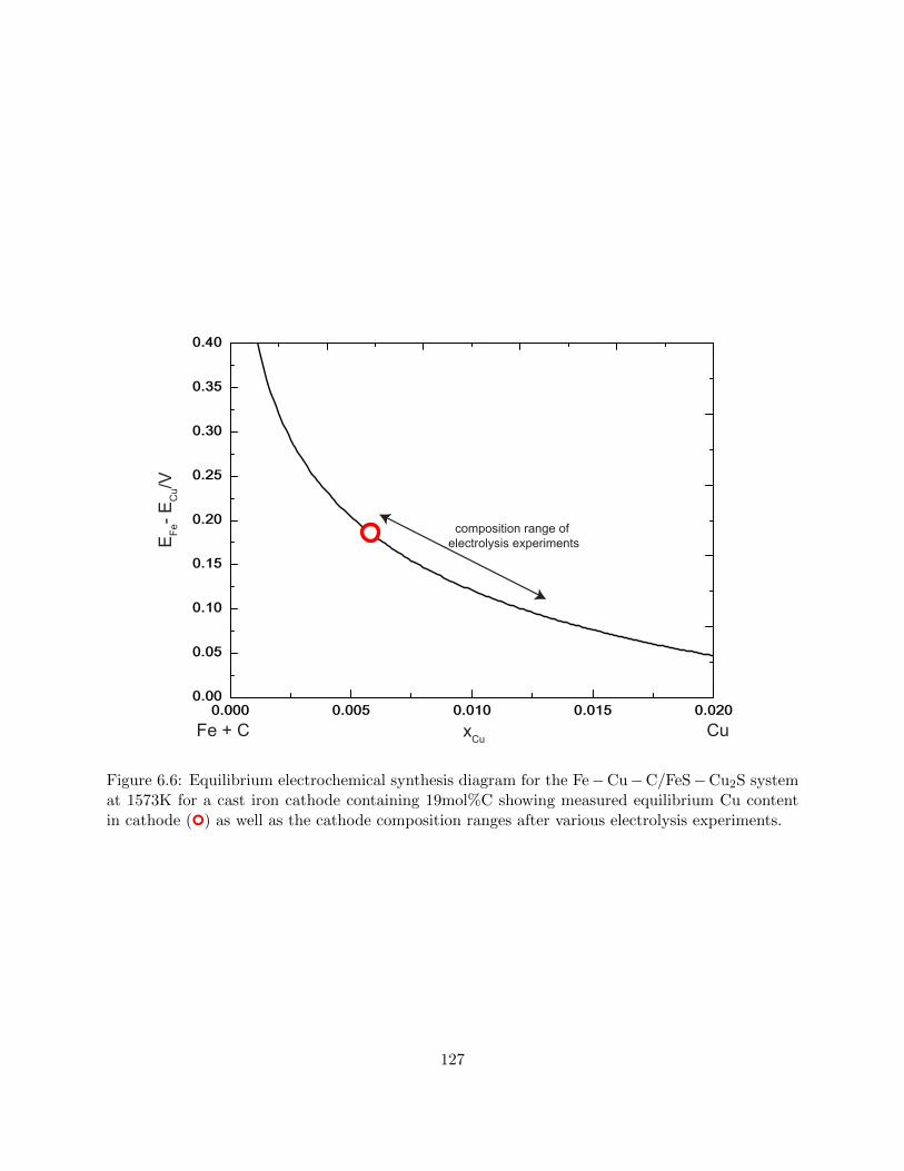
composition range of electrolysis experimentsΕ F
e- Ε C
u/V
Fe + C xCu Cu
Figure 6.6: Equilibrium electrochemical synthesis diagram for the Fe−Cu−C/FeS−Cu2S systemat 1573K for a cast iron cathode containing 19mol%C showing measured equilibrium Cu contentin cathode () as well as the cathode composition ranges after various electrolysis experiments.
127
ideally relative to one another in the electrolyte, rather, there is an energetic drive for the supporting
BaS-La2S3 electrolyte to mix with Cu2S instead of FeS.
During electrolysis, a small variation in Cu content was found for several different experiments.
The Cu composition in the cathode post-electrolysis ranged from 0.6mol% to 1.36mol%. A compar-
ison between cathode composition after equilibration and after electrolysis is shown in Figure 6.6.
6.2.3 Discussion
Overall, very low amounts of Cu were found to alloy in the cast iron cathode. Equilibrium
experiments produced the lowest level of alloying at 0.58mol%. Even accounting for the shift in
electrolyte concentration, this Cu content is still lower than that predicted by an ideal solution
model (approximately 1mol% Cu). Therefore, it can be concluded that FeS and Cu2S interact
differently with the supporting electrolyte. These interactions favor mixing with Cu2S over FeS,
which drives the electrochemical cell towards FeS reduction.
In addition to a preference for Fe deposition due to electrolyte thermodynamics, Fe deposition
is also favored by the cathode chemistry. There is a large positive energy of mixing for Fe and
Cu metal, leading to phase separation in the cathode. This energetic is enhanced by the addition
of C and demonstrates the significant role the cathode can have in influencing an electrochemical
reaction.
More Cu was deposited on the cathode during electrolysis than equilibrium experiments (Fig-
ure 6.6). As in the other electrochemical case studies analyzed with this model, there are several
reasons why this may occur. First, the primary goal of the Fe electrolysis experiments was the
development of a new industrial process to produce Cu metal directly from chalcopyrite. Accord-
ingly, the experiments were run at larger cathode current densities (≈ 1A/cm2). It was shown in
Chapter 4 that larger current densities tend to produce a greater degree of cathode alloying, and
the results of the Fe-Cu separation experiments are consistent with that observation.
In addition, in order to test the tolerance of the system for variations that are common in
industry, but less common in the laboratory, there was variation in both FeS-Cu2S ratios as well
as C content in cast iron between the electrolysis experiments. Both compositional shifts can
128

be expected to influence the true equilibrium Cu content in the cathode. However, comparison of
equilibration results to electrolysis results shows that equilibrium experiments, in combination with
an equilibrium electrochemical synthesis diagram, can be used to define an approximate range of
expected cathode composition, despite small variations in system concentration. This approximate
range could be used to predict the results of electrochemistry. In the case of Fe-Cu-C, this prediction
is more accurate than present methods of estimating electrochemical outcome, which would have
discounted Fe-Cu separation from sulfides as impossible due to their minimal difference in standard
state reduction potential. This is a strong indication that although this model is an equilibrium
model, it has utility in analyzing industrial processes as well as laboratory-scale ones.
6.3 Summary
The difference between Ag2S-Cu2S separation and FeS-Cu2S separation highlights the effect
that solution thermodynamics of both the electrolyte and the cathode have on electrochemical
processes. Despite the decomposition potential difference of Fe and Cu being almost 5 times less
than that between Ag and Cu, both equilibrium and electrolysis experiments tended to produce
greater separation of Fe from Cu than Ag from Cu.
The Ag2S-Cu2S system has a standard state decomposition potential difference of 257mV, but
a strong drive for Ag-Cu alloying in the liquid cathode as well as an electrolyte that tends to
favor mixing with Ag2S over Cu2S. Both of these factors together lead to a greater increase in Cu
deposition than would be expected from standard state thermodynamics alone.
In contrast, the FeS-Cu2S system has a standard state decomposition potential of 54mV. This
alone should indicate that Cu and Fe will be very difficult to separate using molten sulfide electrol-
ysis. However, energetic repulsions between Cu and cast iron, along with an electrolyte that favors
mixing with Cu2S over FeS, lead to less Cu deposition than standard state thermodynamics would
indicate.
Considering the high reactivity of sulfides and their relatively unknown thermodynamic proper-
ties, it would be difficult to come to such a conclusion without relative activity measurements and
129

equilibrium electrochemical synthesis diagrams. Equilibrium electrochemical synthesis diagrams
show directly the influence different cathode concentrations have on a system’s drive to either co-
deposit or separate. Such a method of analysis can be used to iterate quickly through different
possible cathodes in order to find one that best suits the desired electrochemical outcome. For
example, increasing C content in the cathode should enhance electrochemical separation of Cu and
Fe.
Relative activity measured in the Wagner-Allanore reference state allows for the quick ther-
modynamic study of new electrolytes. By only considering the activity of the two species being
investigated for co-deposition, the measurement is intuitive to the electrochemist seeking to quickly
understand if his electrolyte is optimal for his desired result. The sulfide studies in this thesis focus
on the behavior of FeS, Cu2S, and Ag2S in a BaS-La2S3 electrolyte. From a comparatively smaller
amount of experiments than would be necessary for a traditional activity analysis, it was possible
to gain a useful understanding of how the supporting electrolyte interacts with the electroactive
species, and to use this understanding to design future electrochemical experiments.
Further experimentation is necessary in order to determine the effect of concentration on FeS-
Cu2S thermodynamics, as well as to investigate the behavior of other more complex solutions
that are relevant to both electronic waste recycling as well as direct reduction from ore: namely,
FeS-Cu2S-Ag2S thermodynamics.
130
Bibliography
[1] Ailiang Chen et al. “Recovery of Silver and Gold from Copper Anode Slimes”. In: JOM
Journal of the Minerals, Metals and Materials Society 67.2 (2015), pp. 493–502. doi: 10.
1007/s11837-014-1114-9.
[2] J Hait, R K Jana, and S K Sanyal. “Processing of copper electrorefining anode slime:
a review”. In: Trans. Inst. Min. Metall. C. 118.4 (2009), pp. 240–252. doi: 10 . 1179 /
174328509X431463.
[3] W.G Davenport et al. Extractive Metallurgy of Copper. Fourth. Elsevier Science, 2002. isbn:
0-444-50206-8.
[4] Sulata K. Sahu, Brian Chmielowiec, and Antoine Allanore. “Electrolytic Extraction of Cop-
per, Molybdenum and Rhenium from Molten Sulfide Electrolyte”. In: Electrochimica Acta
243 (2017), pp. 382–389. issn: 00134686. doi: 10.1016/j.electacta.2017.04.071.
[5] Samira Sokhanvaran et al. “Electrochemistry of Molten Sulfides: Copper Extraction from
BaS-Cu 2 S”. In: Journal of The Electrochemical Society 163.3 (2016), pp. D115–D120. issn:
0013-4651. doi: 10.1149/2.0821603jes.
131

132
Chapter 7
Predicting Solution Behavior in
Non-Electrochemical Systems: Rare
Earth Magnet Recycling
7.1 Introduction
The overarching goal of this work has been to present an alternative to traditional thermody-
namic modeling methods of high temperature solutions. Although the focus has been primarily on
application to electrolytes, it is critical to note that this is by no means the limit of this approach.
By using the equations of classical thermodynamics to merge select high-quality data with limited
calculations, new insights on any material may be gained. In this chapter, that methodology, which
forms the core of my electrochemical model, is applied to a non-electrochemical system.
As in Chapter 4, the rare earth system is used to verify this approach. Like rare earth electrol-
ysis, the data surrounding rare earth magnet metallurgy is scattered and incomplete. There is no
commercially available CALPHAD model for the complete rare earth magnet system, but certain
binaries and ternaries, for example, Fe-Nd-B and Nd-Pr, have been optimized separately [1–5], with
limited integration of multiple rare earth elements alongside iron and boron. The case is further
complicated by a lack of a solution model able to accommodate both additives (e.g. Al, Ga, Nb)
133

as well as impurities (e.g. C, O, S). In addition, gathering experimental data is hindered because
the process conditions of rare earth magnet production are kept proprietary by the companies that
manufacture them, and so the experimental data available was measured under a variety of different
conditions. While this lack of data may be discouraging for those wishing to perform a traditional
fully computational or experimental analysis, in this chapter I demonstrate how, with the hybrid
approach to modeling, valuable information can still be obtained for the system.
7.2 Motivation
Rare earth magnets of the Fe-R-B type (iron, rare earth, boron) have become increasingly
popular for their use in everything from small electronics to turbines. The rare earth elements in
these magnets are alloyed to achieve a composition of more than 60% iron, producing an iron-rich
microstructure not unlike that of hypoeutectoid steel. In place of pearlite, the large grains are an
Fe-R-B compound phase, called the 2-14 phase for its stoichiometry: Fe14R2B. The 2-14 grains are
separated not by ferrite, but by a metallic rare earth rich solid-solution grain boundary phase [6,
7]. Figure 7.1 shows a schematic of the typical microstructure found in an Fe-R-B type magnet.
Unlike pearlitic steel, this alloy must be rapidly quenched for this microstructure to appear: at low
temperature an iron solution is favored over the Fe14R2B compound. If processed correctly, this
iron-based alloy has demonstrated unique bulk magnetic performances, creating the opportunity
to miniaturize magnets for extremely powerful magnetic fields. Figure 7.2 gives an overview of
the main processing steps involved in Fe-R-B magnet manufacturing. Ultimately, the cast alloy
is jet milled into a fine powder and sintered into its final form. Magnet production, therefore,
incorporates many areas of ferrous metallurgical knowledge, from casting to powder metallurgy. At
the core of this process is the chemistry of the cast alloy. This composition dictates the elemental
distribution in the final microstructure, and in turn, the magnetic performance. As in high-end
steel production, elemental compositions are controlled below a fraction of a weight percent at
casting and problematic impurities like Si and P are kept to an absolute minimum.
In its methods of casting, powder metallurgy, and impurity control, the rare earth magnet in-
134

Figure 7.1: Schematic of a typical Fe-R-B magnet microstructure showing the magnetic 2-14 grainsseparated by a rare earth rich “other metallic phase” at the grain boundaries.
dustry drew inspiration from the technology of the steel industry to improve and expand. However,
rare earth metals have a supply pipeline and market very different from steel because primary
production occurs mostly in one country, China. Because most rare earth mines and smelters are
concentrated in this single country, the market is exposed to the political, environmental, and social
risks that arise from not having sufficient alternative sources readily available in other regions of the
world [8, 9]. In addition to the geographical limitations of mining and processing rare earths, their
chemistry provides other challenges. The rare earths are f-block metals, and can be divided into
two subgroups: light rare earths (lanthanum through samarium) and heavy rare earths (europium
through lutetium). Elements within these subgroups are known for their chemical similarity- a trait
that makes separating these elements difficult. Producing purified rare earths in a primary smelter
is expensive, energy intensive, and creates radioactive and acidic waste that require extensive treat-
ment to mitigate their environmental impact [9]. Despite the issues with primary production, the
development of newer, smaller, and faster electronics push for more virgin material to be mined
and processed. For this reason, the effort to recycle magnets has gained increasing interest recently.
Most efforts for magnet recycling focus on bulk magnet waste, which comes from large decom-
missioned equipment such as turbines. Typically still in one piece, their contamination is often
limited to their surface and they have not reacted much with oxygen. Beyond the traditional hy-
135
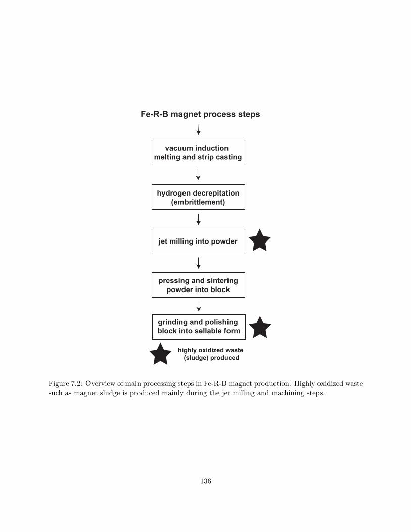
Fe-R-B magnet process steps
vacuum induction melting and strip casting
hydrogen decrepitation(embrittlement)
jet milling into powder
pressing and sinteringpowder into block
grinding and polishing block into sellable form
highly oxidized waste (sludge) produced
Figure 7.2: Overview of main processing steps in Fe-R-B magnet production. Highly oxidized wastesuch as magnet sludge is produced mainly during the jet milling and machining steps.
136

drometallurgical recycling methods, hydrogen reduction [10, 11], chlorination [12], metallothermic
reduction with calcium (Ca) [13] and phase separation with liquid magnesium (Mg) [14] have been
proposed, among others [8]. Magnet sludge created when manufacturing smaller magnets is more
difficult to treat. This is the highly oxidized factory waste produced during jet milling, machining,
and grinding magnets down to their final sellable form (Figure 7.2). Magnet sludge is different
from bulk end-of-life magnets. It has higher levels of oxygen alongside other contaminants from
machining, such as carbon from lubrication. If magnet sludge is recycled, its high levels of oxygen
and other impurities mean it is treated similarly to a mined rare earth ore. Figure 7.3 outlines this
commercial recycling process.
The sludge is first cleaned with acid before being sent back to primary rare earth smelters
where it is mixed with mined ore prior to solvent extraction. Ultimately, pure rare earth metals
are obtained via molten salt electrolysis [8]. During the leaching step, all of the sludge is oxidized,
including portions that may have originally still been metallic. Additional energy is required to
re-reduce these metals to create suitable rare earth metal or alloy feedstock. Despite the challenge
of being highly contaminated, efforts have been made to develop a recycling process targeted
specifically at magnet sludge. Research into these new methods mostly focus on Ca reduction
because of the sludge’s high oxygen levels [13, 15–18].
Recycling sludge by mixing with primary feed aims at recovering the rare earth metal value, and
the end goal is to obtain a purified product that can be sold to downstream production companies
like magnet manufacturers. This strategy may be criticized with two sustainability arguments.
First, if the goal of recycling is to avoid the environmental and economic costs of primary rare
earth production, treating sludge alongside primary feed will link the secondary rare earth content
value to the primary rare earth value. This is analogous to the connection between scrap steel
price and primary steel price. Second, the rare earth sludge is treated as a type of rare earth ore,
when in fact, at greater than 60 wt% Fe, the sludge is closer in elemental composition to a heavily
oxidized scrap iron alloy [18, 19].
Herein, an alternative approach is adopted. Noting the high Fe content, the sludge and magnet
manufacturing wastes are considered as iron-based materials with essentially the correct metal
137
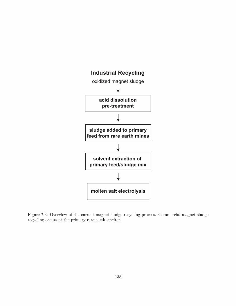
Industrial Recycling
acid dissolutionpre-treatment
sludge added to primaryfeed from rare earth mines
solvent extraction of primary feed/sludge mix
molten salt electrolysis
oxidized magnet sludge
Figure 7.3: Overview of the current magnet sludge recycling process. Commercial magnet sludgerecycling occurs at the primary rare earth smelter.
138

composition needed to produce a magnet, and a process for producing a magnet directly from
such wastes is explored. As in earlier chapters, modeling the underlying chemical thermodynamics
enables a new perspective on materials processing. Therefore, a comprehensive thermodynamic
assessment of two parts is proposed. In the first, the reaction of magnet sludge with oxygen is
modeled. In the second, the reduction energy needed to remove this oxygen and return the magnet
back to its original composition is estimated. Although magnet sludge is also contaminated by
cutting media and lubricant, studies dedicated to sludge recycling have shown promising results in
cleaning away these impurities, which are not typically chemically bonded to the magnet [16, 18].
Since oxygen chemically reacts with the metals in the magnet, it poses a true chemical metallurgy
challenge to recycling. Thus, treating oxygen is the focus of this chapter. In absence of a complete
solution model able to accommodate all elements present in a typical magnet, thermodynamic
calculations herein involve only standard state Gibbs energies of pure components and compounds.
Using standard state to study oxidation has a rich history in ferrous thermodynamics in the form
of Ellingham and Kellogg diagrams, which both relate the oxidation behavior of a pure metal or
compound to the atmosphere and temperature of its environment.
7.3 Magnet Sludge Model
7.3.1 Modeling Methodology
The “Equilib” module of FactSage 7.3 was used to minimize the Gibbs energy and predict
which pure components and compounds were stable under a given temperature and pressure. The
standard-state elements and compounds used were divided into three phase subgroups:
1. the magnetic “2-14” phase consisting of Fe14R2B where R may be Pr, Nd, or Dy;
2. the “other metallic” phase, which consists mostly of rare earths along with additives and
impurities that make up the intergrain region between the 2-14 phase [6, 20]
3. any oxides present.
The “other metallic” phase was modeled using the FactPS database in FactSage [21], with the
139

exception of R-B compounds, R-Fe compounds, and non 2-14 Fe-R-B compounds [22]. The oxide
phase was modeled using FactPS and Fe-R-B-O compounds optimized by Jakobsson et. al [23].
The 2-14 phase has been reported to initially oxidize less than other magnet components [24, 25].
This limited oxidation did not appear to be accounted for in published thermodynamic models [1,
3, 4], and so herein is assumed to be of a kinetic origin. In order to account for this behavior
and add this constrain on phase stability, the ∆Hf for Fe14Pr2B, Fe14Nd2B, and Fe14Dy2B were
modified from their originally optimized values [1, 3, 4]. For each compound, ∆Hf was lowered by
increments of 10 kJ until overall 2-14 phase formation was favored over competing Fe-intermetallics,
e.g. Fe2Ti. The Gibbs energy functions for the modified compounds are presented in Table 7.1.
Initial Melting of the Rare Earth Magnet
As most magnet producers use proprietary alloy concentrations, a detailed compositional anal-
ysis of feedstock for magnet production could not be found. Lixandru et. al. [19] measured the
major and minor elements contained in laptop speaker magnet waste through ICP-OES: Fe, Nd,
Pr, Dy, Gd, Co, Nb, Cu, Al, Ga, Zn, B. The average composition measured fell within the range
suggested by prior art [6]. Therefore, these published results inform the basis of the present case
study. In order to include the contribution of impurities, four main feedstocks were identified: elec-
trolytic iron, ferroboron, ferroniobium, and praseodymium-neodymium alloy. Commercial sources
of these feedstocks often disclose the composition of impurities such as O and C, and impurity
levels often vary depending on feed grade and source. The commercial sources used were chosen on
the basis of report thoroughness and overall purity: a source that disclosed O, C, Si, and P content
would be chosen over a source that only disclosed C content. When deciding between two equally
well-detailed sources, the one with the lowest impurity content was chosen to reflect a magnet
manufacturing strategy based on premium material grades. The impurity compositions found in
this manner were then added to the total mass balance [26–28]. This method worked well for all
elements except for Si and P. Their estimated weight percent in the initial mass balance was so high
they impeded formation of the 2-14 phase, and as such their amounts in the final mass balance were
reduced to 10% of their originally estimated value. From a ferrous metallurgy consideration, it can
140
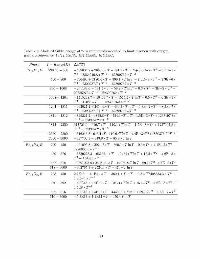
Table 7.1: Modeled Gibbs energy of 2-14 compounds modified to limit reaction with oxygen.Real stoichiometry: Fe(14.00018), R(1.99988), B(0.9994)
Phase T −Range(K) ∆G(T )
Fe14Pr2B 298.15− 500 −489604.7 + 2668.6 ∗ T − 491.2 ∗ T lnT + 8.3E−2 ∗ T 2− 5.1E−5 ∗T 3 + 3334946.8 ∗ T−1 − 62399762 ∗ T−2
500− 800 −466493 + 2120.4 ∗ T − 399.1 ∗ T lnT − 7.3E−2 ∗ T 2 − 3.3E−6 ∗T 3 + 2320237.7 ∗ T−1 − 62399762 ∗ T−2
800− 1068 −261189.6 − 191.5 ∗ T − 59.8 ∗ T lnT − 0.3 ∗ T 2 + 3E−5 ∗ T 3 −20855972 ∗ T−1 − 62399762 ∗ T−2
1068− 1204 −1415268.7 + 10423.7 ∗ T − 1565.5 ∗ T lnT + 0.5 ∗ T 2 − 6.3E−5 ∗T 3 + 1.4E8 ∗ T−1 − 62399762 ∗ T−2
1204− 1811 −492027.2 + 2410.9 ∗ T − 439.3 ∗ T lnT − 6.3E−2 ∗ T 2− 8.3E−7 ∗T 3 + 2320237.7 ∗ T−1 − 62399762 ∗ T−2
1811− 1812 −849221.2+4855.8∗T −754.1∗T lnT −1.5E−3∗T 2 +1237197.8∗T−1 − 62399762 ∗ T−2
1812− 2350 317721.9− 619.7 ∗ T − 110.1 ∗ T lnT − 1.5E−3 ∗ T 2 + 1237197.8 ∗T−1 − 62399762 ∗ T−2
2350− 2800 −316246.8−615.1∗T−110.6∗T lnT−1.4E−3∗T 2+1830376.6∗T−1
2800− 3000 −397703.3− 843.8 ∗ T − 85.9 ∗ T lnT
Fe14Nd2B 200− 450 −491095.8 + 2024.7 ∗T − 360.1 ∗T lnT − 0.3 ∗T 2 + 4.1E−5 ∗T 3−1226885.5 ∗ T−1
450− 576 −3359228.3 + 63255.1 ∗ T − 10474 ∗ T lnT + 15.5 ∗ T 2 − 4.6E−3 ∗T 3 + 1.5E8 ∗ T−1
567− 618 −9697023.9+264314.3∗T−44496.2∗T lnT+69.7∗T 2−1.8E−2∗T 3
618− 3000 −462765.3 + 2524.3 ∗ T − 470 ∗ T lnT
Fe14Dy2B 298− 450 2.2E13 − 1.1E11 ∗ T − 360.1 ∗ T lnT − 0.3 ∗ T 2408333.3 ∗ T 3 +1.2E−4 ∗ T−1
450− 592 −5.3E13 + 1.4E11 ∗T − 10474 ∗T lnT + 15.5 ∗T 2− 4.6E−3 ∗T 3 +1.5E8 ∗ T−1
592− 616 −5.3E13 + 1.4E11 ∗T − 44496.1 ∗T lnT + 69.7 ∗T 2− 1.8E−2 ∗T 3
616− 3000 −5.3E13 + 1.4E11 ∗ T − 470 ∗ T lnT
141

be assumed that advanced magnet producers would source specialty feed low in Si and P content.
Gd, Dy, Cu, Al, Ga, Zn, and Co were present at such low concentration that any impurities in
their respective feedstock were neglected. Table 7.2 summarizes the composition of the feedstocks
and initial input used in this case study.
This initial input was allowed to equilibrate at 1723 K and 0.5 bar Ar containing 1ppm O2, CO
and H2O; and 5ppm N2 [29] using FactSage’s Equilib software. This step simulated the conditions
in the vacuum induction melting (VIM) furnace, the first step in magnet production. Temperature
and atmospheric conditions were taken from prior art [6, 20]. The results after the melting step
are presented in Table 7.2. This high temperature step refined the magnet composition, as species
were allowed to volatilize off and react with oxygen impurities in the Ar atmosphere.
Strip Casting Kinetic Simulation
In practice, as illustrated in Figure 7.4, after a magnet is melted in the VIM, it is rapidly cooled
via strip casting. This rapid cooling inhibits the formation of ferrite and promotes the 2-14 phase
instead. As in other rapid cooling methods of ferroalloys, carbon rejection and graphite precipitation
are also prevented. The lack of ferrite and graphite creates a metastable alloy. FactSage allows for
modeling of kinetically metastable phases by enabling the user to “de-select”, or suppress certain
phases. If suppressed, the “de-selected” phase will not form and the next stable phase will form
instead. An instructive example can be seen in steel modeling. If graphite is suppressed, cementite
will form instead. To obtain the metastable phases created through rapid cooling, herein all pure
Fe and pure C phases were selected as “suppressed” phases and were not allowed to form. This
led to the formation of iron compounds and carbides. To further simulate rapid cooling, no gas
evolution was allowed. It was at this point in the model that the modified 2-14 compounds were
incorporated in order to account for their kinetic stability. A full comparison between industrial
practice and our results is presented in Figure 7.4.
142

Table 7.2: Elemental compositions used for calculations with no additional oxygen. Initial: com-positions estimated from published reports. Post-V IM : calculated after “initial” composition wasequilibrated at 1723K to simulate treatment in vacuum induction melting furnace.
Element Initial Post-V IM(wt %) (wt %)
Pr 6.69% 6.72%
Nd 23.46% 23.59%
La 0.02% 0.02%
Ce 0.02% 0.02%
Fe 65.06% 65.41%
Al 0.66% 0.66%
Si 0.01% 0.01%
Mo 0.02% 0.02%
W 0.02% 0.02%
Ti 0.02% 0.02%
Ca 0.003% 0.002%
Mg 0.01% 0.00%
S 0.01% 0.01%
C 0.02% 0.02%
B 0.96% 0.96%
P 0.01% 0.01%
Mn 0.06% 0.05%
Cr 0.005% 0.005%
O 0.09% 0.09%
Nb 0.05% 0.05%
Ta 4E−5% 4E−5%
Dy 1.67% 1.67%
Gd 0.06% 0.06%
Co 0.44% 0.45%
Cu 0.12% 0.12%
Ga 0.05% 0.04%
Zn 0.50% 0.00%
143

Industrial Practice
VIM1573-1773 K
vacuum or inert atmosphere
Fe, R, B +contaminants & additives
rapid cooling stripcasting to inhibit
ferrite and promote2-14 phases
cast magnet flakeat least 80vol% 2-14
R-rich intergrainminimal oxidation
Thermodynamic ModelFe, R, B +
contaminants & additives
FactSage Equilib1723K, 0.5 bar Ar
no elementssuppressed
289 K, 1 barpure Fe, C and all
gasses suppressedweighted 2-14 phase
calculated baselinephase distribution
90.62wt% 2-148.72wt% intergrain
0.65wt% oxide
Figure 7.4: Comparison between actual magnet manufacturing (left) and the modeling steps usedherein (right).
144

Oxidation Model
The elemental oxygen content in the condensed phases present post-furnace were incrementally
increased, with a total O content ranging from 0.1wt% to 5.4wt%. The ratios of all other elements
were kept constant. New phases were calculated using Equilib at 298 K with gas phases and all
pure Fe (ferrite) and C (graphite) phases suppressed. The kinetically modified 2-14 compound data
were used, and the Fe14Pr2B phase was suppressed. Fe14Pr2B was not predicted form in the initial
case without added oxygen, and so it was assumed it could not reasonably form on its own at
298K with an increase in oxygen. Because the model was based in standard-state thermodynamics
using only compounds and pure elements, no model for dissolved oxygen was used. All oxygen was
modeled as incorporated in an oxide compound phase.
7.3.2 Results
Simulated Magnet after Melting and Casting
The output from the VIM model at 1723K and 0.5 bar Ar shows minor changes to the overall
magnet composition. Most notably, all of the Zn and Mg were predicted to volatilize off. Starting
with one tonne of initial feedstock, 107g Mn, 64g Ga, 11g Dy, 9g Ca, 3g Cu, and 2g Nd also
volatilized off. This new composition (Table 7.2) was then used to calculate the baseline phase
distribution.
Figure 7.5 shows the calculated weight percent of each phase (oxide, 2-14, and “other metallic”)
and Figure 7.6 shows the distribution of each rare earth element among these three phases. The
oxide phase, present overall at 0.65%, is comprised of Gd2O3 and Nd2O3. The 2-14 phase, at 90.63%,
consists of Fe14Nd2B and Fe14Dy2B. Finally, the “other metallic” phase, with the remaining rare
earth and boron, additives, and impurities, contains GdS, Ce2C3, Nd2B5, LaC2, Pr, Nd, and PrAl2,
among other non-rare-earth containing compounds. The model inputs and outputs at each stage
in the baseline calculation are given in detail elsewhere [30].
145

Figure 7.5: Calculated phase distribution in the simulated magnet after melting and casting withno additional oxygen added (baseline case).
Figure 7.6: Modeled distribution of rare earth elements among phases in baseline case. Rareearth containing phases present: Dy: 100% Fe14Dy2B, Ce: 100% Ce2C3, Nd: 2% Nd2O3, 96%Fe14Nd2B, 2% Nd2B5 Pr: 82% Pr and 18% PrAl2, La: 100% LaC2, Gd: 14% Gd2O3, 86% GdS.
146

Figure 7.7: Calculated changes in phases present as oxygen content is increased from 0.09wt% to5.4wt%. l: 2-14 phase, s: “other metallic” grain boundary phase, n: oxide phase. After thegrain boundary phase is completely oxidized near 1.8wt%, the 2-14 phase begins to break downinto oxide and more metallic phases.
Addition of Oxygen
Oxygen was incrementally added to the magnet until 5.4wt% O was achieved. As the oxygen
content increases, the predicted phase distribution changes, as presented in Figure 7.7. The rare
earth elements in the “other metallic” intergrain phase oxidize at the lowest levels of oxygen,
converting into oxide until the “other metallic” phase drops from 8.1% to 0.8wt% at 1.8% O. At
this oxygen level, the 2-14 phase begins to decompose into oxide and various metallic phases. The
2-14 phase continued to decrease with increasing O, until it became the minor phase: 15.2% at
5.4%O.
Figure 7.8 shows that for an oxygen content of 5.4%, the distributions of rare earths among the
phases change significantly from the baseline case (Figure 7.6). The heavy rare earths, Dy and Gd,
are completely oxidized, while some of the lighter rare earths, most notably Nd and Pr, remain in
a metallic state bonded with Fe. Overall, 40% of the rare earth elements by weight are oxidized,
while 60% remain in the metallic phase.
147

Figure 7.8: Modeled distribution of rare earth elements among phases with 5.4wt% O present.Rare earth containing phases present: Dy: 100% Dy3Al5O12 Ce: 15% CeO2 85% CeCrO3 Nd: 2%Nd3Al5O12, 45% NdBO3, 18% Fe14Nd2B, 35% Fe8Nd Pr: 100% Fe8Pr Gd: 100% Gd3Al5O12
7.3.3 Discussion
Melting and Casting Model Performance
The initial, post-furnace composition of the magnet used in the simulation was estimated to
contain 0.09% O and 0.02% C. This calculated oxygen level is below that reported for finished mag-
net products [7, 18]. It has been observed that oxygen levels in a magnet increase during processing,
particularly during the powder metallurgy steps [24]. Predicting a cast alloy oxygen content below
the level in sintered magnets indicates sufficient performance of the proposed VIM model. The
carbon level 0.02% was also just below the experimentally measured values of 0.03% [18].
In order to produce a material with magnetic performances to the specifications of prior art,
the 2-14 phase should comprise at least 80% of the rare earth magnet by volume, and the “other
metallic” grain boundary phase should be rare earth rich [6, 20, 25]. A weight fraction of 90.63%
for the 2-14 phase was predicted by the initial casting model. The “other metallic” phase predicted
by the model was 82.5% rare earth. Both the initial magnet composition and modeled phase
distribution show good agreement with experimental data available in literature, supporting the
148
validity of the casting model, and, in a more general sense, the utility of a thermodynamics-based
analysis even when the available data is not complete.
Oxidation Model Performance
The magnet oxidation model results in Figure 7.7 show two important O compositions. First,
at 0.8% O, the phase fraction of oxide overtakes the phase fraction of the grain boundary. In his
study of FeNdB magnet recycling, Lalana noted both virgin and recycled magnets appear to reach
an equilibrium oxygen concentration of 0.55% [24]. Kim et. al found that magnets with O levels
greater than 0.6% showed a higher resistance to further oxidation [31]. These observations suggest
a barrier preventing the magnet from easily up-taking oxygen near 0.55%-0.6%. The crossover near
0.8% in Figure 7.7 indicates that such a barrier may be reproduced with the sole use of chemical
thermodynamics.
The second important composition in Figure 7.7 is at 1.8% O, above which the 2-14 composition
breaks down significantly. It is well-documented that the 2-14 phase remains stable until a signif-
icant portion of the intergrain region has been oxidized. At this point the 2-14 phase decomposes
into iron and rare earth oxide [24, 25]. The model results show a similar behavior, demonstrating
agreement with experimental literature. A phase fraction of 80% by volume for the 2-14 phase is
considered to be the threshold to achieve satisfactory magnet performance [25]. Past this threshold,
the magnet likely becomes unusable and must be either sent to landfill or recycled alongside oxide
feed at the smelter. Our chemical thermodynamic results thus explain the difficulties with recycling
heavily oxidized magnet material [8]. Eventually, at 3.6%, most of the 2-14 phase has decomposed
into rare earth oxide and metallic iron.
The model’s agreement with literature supports the utility of the weighted 2-14 phases. By
lowering ∆Hf of 2-14 compounds until their formation was favored over competing ferrous inter-
metallics, the correct phase distribution was achieved without needing to “suppress” those inter-
metallic phases. This enabled them to re-emerge as oxygen content was increased and the 2-14 phase
decomposed. If all competing phases were suppressed instead, the 2-14 phase would not decompose
and the magnet would saturate in oxygen before reaching 5.4% O, an outcome in contradiction
149
with literature [16, 18, 32].
7.4 Recycling Model
The thermodynamic model has shown good agreement with available literature, both to re-
produce melting and casting behavior at low oxygen content, and to predict the effects of higher
oxygen content (oxidation) on magnet waste. With both low oxygen and high oxygen cases pre-
dicted accurately solely by thermodynamic means, we can confidently extend this approach to an
unstudied area, as we did in Chapter 6. Herein, we use a thermodynamic-based analysis to evaluate
and compare the feasibility of possible recycling pathways.
7.4.1 Modeling Methodology: Oxygen Removal
In order to remove oxygen, herein modeled as oxide compounds, it was necessary to calculate
the chemical (Gibbs) energy required to reduce the oxide phases to metal and oxygen gas. This ∆G
decreases with increasing temperature for metal oxides. This energetic benefit with temperature is
offset by the energy (enthalpy) cost of heating the sludge, ∆H. Both ∆G and ∆H were considered.
First, condensed phases obtained from the 5.4wt% oxidation model were allowed to reach internal
equilibrium at room temperature. Pure Fe and pure C phases were allowed, and unweighted 2-
14 phases were used. This simulated the changes in the sludge during the pre-reduction steps
and heating from room temperature to the target reduction temperature. At a finite temperature
above room temperature, it is expected that the oxidized sludge will reach internal equilibrium,
redistributing C, O, Fe, and R across the most stable phases. Once equilibrated, ∆H was calculated
as the energy required to heat the newly equilibrated material to processing temperature. ∆G was
found as the energy required to completely decompose the oxidized sludge to metal + (O, O2,
and O3) at the processing temperature. Other gas phases such as CO, CO2, and SO2 were also
permitted, but gaseous metal oxides were not. When calculating the amount of energy needed
to remove O completely from the magnet, 5.4 wt% O was chosen as the starting total oxygen
content in the sludge. This level was similar to experimentally measured values available in the
150
literature [16, 18, 32].
7.4.2 Reduction Thermodynamics Results
In the study of energy needed to reduce all of the oxides contained in the 5.4wt% O sludge, two
different case studies were considered:
1. the energy to heat and reduce only the rare earth oxides initially contained in magnet sludge,
assuming that the rare earth oxides were first separated from the rest of the waste prior to
treatment.
2. the energy to heat and reduce 1 tonne of simulated waste material at 5.4wt% O.
Figure 7.9 compares these two cases, looking first at the ∆G to reduce the material and second at
how ∆H influences the energy requirements. For consistency, all cases have been normalized by
the mass of oxidized rare earth metal present in each case. This normalization was chosen so the
results could be easily compared with analyses of existing recycling methods [9, 33].
For Case 1, which models the case where rare earth oxides would be first separated from the
magnet before reduction, the amount of oxidized rare earth is fixed at 0.123 tonne RE/tonne waste.
For Case 2, which models the entire magnet waste (including rare earth metals not oxidized initially
due to kinetics), the amount of oxidized rare earth at equilibrium varies with temperature. It can
be seen in Figure 7.9 that less energy is needed to reduce the rare earth oxides if reduced alongside
the rest of the magnet waste than to reduce the rare earth oxides alone. This is true regardless if
∆H is considered. If ∆H is considered, the benefit to reducing the entire magnet waste is lessened
at higher temperatures as more energy is expended to heat the whole magnet as opposed to just the
oxidized fraction. Above 2000K a crossover point will occur where it is more energetically favorable
to treat only the oxides.
Figure 7.10 shows the predicted phase distribution at 1773K as simulated magnet waste is
deoxidized from 5.4%O to 0%O. Fe-rich metallic phases containing no rare earths and oxide phases
containing mostly rare earth oxides are the dominating phases at 5.4%O. As deoxidation proceeds,
the newly reduced rare earth metals combine with iron to form Fe-R metal compounds such as
151
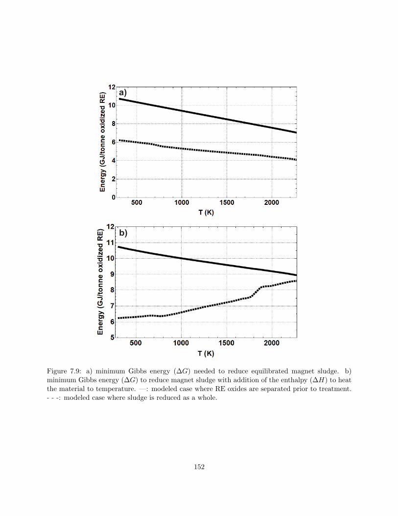
a)
b)
Figure 7.9: a) minimum Gibbs energy (∆G) needed to reduce equilibrated magnet sludge. b)minimum Gibbs energy (∆G) to reduce magnet sludge with addition of the enthalpy (∆H) to heatthe material to temperature. —: modeled case where RE oxides are separated prior to treatment.- - -: modeled case where sludge is reduced as a whole.
152

Figure 7.10: Calculated changes in phases present as O content in magnet sludge is reduced from5.4% to 0% at 1773K. s: rare earth rich metallic phase (no Fe), n: oxide phase , l: metallic phasescontaining Fe and rare earth, u: Fe-rich metallic phase (no rare earth). As oxygen is removed, Feand rare earths interact to create new phases.
Fe17R2 and Fe4RB4. Eventually these compounds become the dominating phases.
7.4.3 Implication for Magnet Sludge Recycling Technologies
In the most highly oxidized case of 5.4%O, rare earth elements are only 30wt% of the magnet,
and 89% of the remaining material is iron. Although past recycling efforts have focused on pro-
cessing the material from a rare earth perspective, bearing in mind that magnet scrap is Fe-rich
may offer new outlooks on its end of life treatment and is the core focus of this case study. From a
purely energetic standpoint, as shown in Figure 7.9, less energy is needed to reduce the rare earths
if they are treated alongside the entire magnet material than to reduce only the rare earth oxide.
This benefit results from favorable interactions between iron and rare earth metals. If only oxidized
rare earths are treated, no iron is present. Instead, if iron is kept, Fe-R compounds are quick to
form as the rare earth is deoxidized as shown in Figure 7.10. The two competing reactions can be
described as:
153

2
yRxOy →
2x
yR+O2 (7.1)
2
yRxOy + zFe→ FezR 2x
y+O2 (7.2)
where ∆G 7.2 < ∆G 7.1 at the processing temperatures considered. It is important to note that
at 1773K, the temperature of the deoxidation analysis in Figure 7.10, the magnet should be mostly
liquid [24]. Because herein we do not account for liquid solution behavior, there is no depression
of the melting point and thus the model considers mostly solids alongside liquid compounds with
a standard state melting temperature below 1773K. For example, the stable form of pure iron at
1773K is BCC solid, and so all of the pure iron in the model at 1773K is considered to be BCC.
It is well-known in thermodynamics that metals which are ordered compounds in the solid state
immediately below their melting point will display short-range ordering at the stoichiometry of the
compound in the liquid immediately above the melting point. Although Fe17R2 will not exist in
the liquid state, favorable interactions between iron and rare earth will remain after melting, and
thus despite these approximations the model still informs trends in energy requirements during
deoxidation.
Reducing the entire magnet material carries another benefit: no additional energy for mechani-
cal or hydrometallurgical separation is required. This separation energy is significant. An estimated
average 19.2 GJ/tonne rare earth is required to operate the hydrometallurgical pumps needed to
separate rare earth species to prepare them for molten salt electrolysis [33]. Including the cost of
water treatment and the energy needed for solvent handling and consumption, LCA analyses for
hydrometallurgical treatment have estimated a contribution of 58 GJ/tonne rare earth to the foot-
print of rare earth processing [34]. We can calculate the energy required for molten salt electrolysis
of one mole of rare earth metal using the Nernst equation:
∆V = −∆G
nF(7.3)
154

where ∆V is estimated as a theoretical minimum of around 4.0 volts and the metal ion valency
n is assumed to be 3 [33]. A molar mass of 144.5 g/mol rare earth mix is calculated using the
relative concentrations of Dy, Ce, Nd, Pr, La, and Gd present in this case study. This predicts a
theoretical minimum of 8 GJ/ tonne rare earth required for electrolytic production of rare earth
metals. Combining the theoretical minimum energy requirements for hydrometallurgical treatment
(19.2 GJ) and for electrolysis (8 GJ) gives a total estimate of at least 27.2 GJ/tonne rare earth
required for the traditional processing route shown in Figure 7.3.
This value can be compared to the range of 6-9 GJ/tonne rare earth required for heating
and reducing magnet sludge whole (Figure 7.9). This estimate is similar in magnitude to the
electrolysis minimum, suggesting that most of the energetic savings can be gained by avoiding
elemental separation and hydrometallurgical treatment. Figure 7.11 shows what such a direct
processing route could look like. Accounting for enthalpy, it can be seen in Figure 7.9 that between
1800K and 1900K, ∆H increases with temperature due to melting and boiling of various elements.
These results indicate an optimal temperature for a bulk magnet recycling process near 1700K,
where the ∆G requirements are low but the ∆H costs have not yet started to sharply increase.
Table 7.3 compares the existing sludge recycling process to the energetics needed to completely
remove the oxygen from the magnet at 1700K. Eliminating the hydrometallurgical step and reducing
the material directly would result in an estimated minimum energy saving of 78%.
The direct reduction of magnet sludge would be a streamlined “magnet-to-magnet” recycling
method. Rather than completely break down and separate the waste into its 25+ elements, only
to be re-mixed into a new magnet, one can envision a route (Figure 7.11) where the waste is
treated whole. Only minor elemental additions would be necessary to correct the stoichiometry
to be commercially acceptable. Furthermore, the optimal temperature, 1700K, is near the 1723K
temperature used in the initial melting and casting step, and within the range proposed by various
patents [6, 20, 25]. One can envision a unified process where the recycled material is reduced in-situ
before being directly cast into a new magnet.
Metallothermic reduction is one possible high-temperature deoxidation method. Figure 7.12
shows the ∆G to reduce the rare earths present in this case study. La and Ce, which require
155

Whole Sludge Recycling
cleaning pre-treatmentto remove lubrication
high temperaturereduction
oxidized magnet sludge
Figure 7.11: Steps for direct recycling of magnet sludge.
156
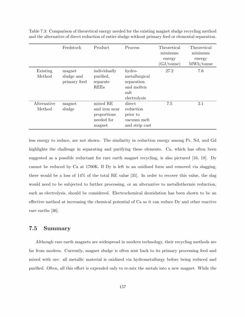
Table 7.3: Comparison of theoretical energy needed for the existing magnet sludge recycling methodand the alternative of direct reduction of entire sludge without primary feed or elemental separation.
Feedstock Product Process Theoreticalminimum
energy
Theoreticalminimum
energy(GJ/tonne) MWh/tonne
ExistingMethod
magnetsludge andprimary feed
individuallypurified,separateREEs
hydro-metallurgicalseparationand moltensaltelectrolysis
27.2 7.6
AlternativeMethod
magnetsludge
mixed REand iron nearproportionsneeded formagnet
directreductionprior tovacuum meltand strip cast
7.5 2.1
less energy to reduce, are not shown. The similarity in reduction energy among Pr, Nd, and Gd
highlights the challenge in separating and purifying these elements. Ca, which has often been
suggested as a possible reductant for rare earth magnet recycling, is also pictured [16, 18]. Dy
cannot be reduced by Ca at 1700K. If Dy is left in an oxidized form and removed via slagging,
there would be a loss of 14% of the total RE value [35]. In order to recover this value, the slag
would need to be subjected to further processing, or an alternative to metallothermic reduction,
such as electrolysis, should be considered. Electrochemical deoxidation has been shown to be an
effective method at increasing the chemical potential of Ca so it can reduce Dy and other reactive
rare earths [36].
7.5 Summary
Although rare earth magnets are widespread in modern technology, their recycling methods are
far from modern. Currently, magnet sludge is often sent back to its primary processing feed and
mixed with ore: all metallic material is oxidized via hydrometallurgy before being reduced and
purified. Often, all this effort is expended only to re-mix the metals into a new magnet. While the
157
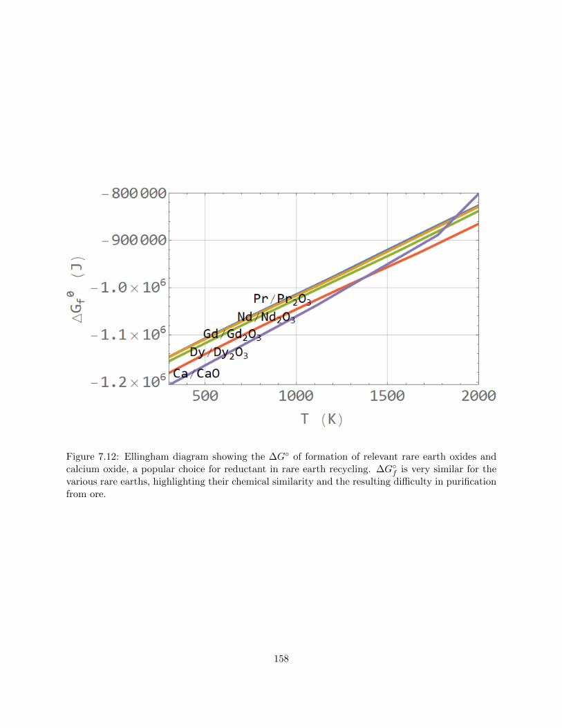
Figure 7.12: Ellingham diagram showing the ∆G of formation of relevant rare earth oxides andcalcium oxide, a popular choice for reductant in rare earth recycling. ∆Gf is very similar for thevarious rare earths, highlighting their chemical similarity and the resulting difficulty in purificationfrom ore.
158

heavy environmental cost of rare earth processing is well-known, and is the source for significant
drive to develop greener methods, innovation is hindered by a fundamental lack of data. Without
an understanding of the chemical interactions in the rare earth magnet system, it is difficult to
know a priori if a new recycling path is viable. By making use of what is known about the rare
earth magnet system, and combining this information with the fundamental equations of chemical
thermodynamics, new understandings of the system may come to light. In turn, this will allow for
experimentalists to gather more targeted data, feeding even more precise predictions.
The rare earth magnet case study is an instructive example into the utility of this approach.
In absence of a full model detailing the interactions of all 25+ elements typically found in a rare
earth magnet, a hybrid model based in standard state classical thermodynamics was adopted.
Through this, the behavior of magnet material as it is melted in the VIM and as it oxidizes
during sludge production could be accurately represented. Comparison with literature shows correct
prediction of certain phenomena, such as delayed breakdown of the 2-14 phase and correlation of
oxidation resistance to oxygen saturation of non 2-14 phases. By extending the modeling effort into
screening for possible recycling technologies, it was predicted that significant energy savings (78%)
could arise if magnet separation and purification steps are skipped in favor of reducing the sludge
whole. An early screen of possible alternatives was conducted: it was found that Ca reduction or
electrochemical deoxidation are promising pathways for more sustainable magnet recycling. Further
work should continue to use this methodology to continue screening for alternatives, and to advise
further experimentation on the subject.
159
Bibliography
[1] Marie-Aline Van Ende and In-Ho Jung. “Critical thermodynamic evaluation and optimization
of the Fe-B, Fe-Nd, B-Nd and Nd-Fe-B systems”. In: Journal of Alloys and Compounds 548
(2013), pp. 133–154. doi: https://doi.org/10.1016/j.jallcom.2012.08.127. url:
http://dx.doi.org/10.1016/j.jallcom.2012.08.127.
[2] B Hallemans, P Wollants, and J.R. Roos. “Thermodynamic Assessment of the Fe-Nd-B Phase
Diagram”. In: Journal of Phase Equilibria 16.2 (1995), pp. 137–49. doi: https://doi.org/
10.1007/BF02664851. url: https://link.springer.com/content/pdf/10.1007%7B%5C%
%7D2FBF02664851.pdf.
[3] Marie-Aline Van Ende et al. “Thermodynamic optimization of the Dy–Nd–Fe–B system and
application in the recovery and recycling of rare earth metals from NdFeB magnet”. In:
Green Chemistry 17 (2015), pp. 2246–62. doi: https://doi.org/10.1039/c4gc02232g.
url: www.rsc.org/greenchem.
[4] Taili Chen et al. “Experimental investigation and thermodynamic description of the Pr–Fe–B
system”. In: Journal of Magnetism and Magnetic Materials 497 (Mar. 2020), p. 165983. issn:
03048853. doi: https://doi.org/10.1016/j.jmmm.2019.165983.
[5] Jacob Wesley McMurray. “Thermodynamic Assessment of the Pr–O System”. In: Journal of
the American Ceramic Society 99.3 (Mar. 2016). Ed. by W. Wong-Ng, pp. 1092–1099. issn:
0002-7820. doi: https://doi.org/10.1111/jace.14049. url: https://onlinelibrary.
wiley.com/doi/abs/10.1111/jace.14049.
160
[6] Takuya Onimura and Shinya Tabata. Method for producing alloy cast slab for rare earth
sintered magnet. 2018.
[7] Elisa Isotahdon. “Corrosion Losses, Mechanisms and Protection Strategies for Sintered Nd-
Fe-B Magnets Citation Isotahdon”. PhD thesis. Tampere University of Technology, 2017,
p. 91. url: http://www.tut.fi/tutcris.
[8] Osamu Takeda and Toru H. Okabe. “Current Status on Resource and Recycling Technology
for Rare Earths”. In: Metallurgical and Materials Transactions E 1 (June 2014), pp. 160–
173. issn: 2196-2936. doi: https://doi.org/10.1007/s40553-014-0016-7. url: http:
//link.springer.com/10.1007/s40553-014-0016-7.
[9] Jason C.K. Lee and Zongguo Wen. “Rare Earths from Mines to Metals: Comparing Environ-
mental Impacts from China’s Main Production Pathways”. In: Journal of Industrial Ecology
21.5 (Oct. 2017), pp. 1277–1290. issn: 10881980. doi: https://doi.org/10.1111/jiec.
12491. url: http://doi.wiley.com/10.1111/jiec.12491.
[10] M. Zakotnik et al. “Hydrogen Decrepitation and Recycling of NdFeB-type Sintered Magnets”.
In: Journal of Iron and Steel Research International 13.Supplement 1 (2006), pp. 289–296.
issn: 1006706X. doi: https://doi.org/10.1016/S1006-706X(08)60197-1.
[11] A. Walton et al. “The use of hydrogen to separate and recycle neodymium-iron-boron-type
magnets from electronic waste”. In: Journal of Cleaner Production 104 (2015), pp. 236–241.
issn: 09596526. doi: https://doi.org/10.1016/10.1016/j.jclepro.2015.05.033. url:
http://dx.doi.org/10.1016/j.jclepro.2015.05.033.
[12] T. Uda. “Technique for Enhanced Rare Earth Separation”. In: Science 289.5488 (2000),
pp. 2326–2329. issn: 00368075. doi: 10.1126/science.289.5488.2326.
[13] Ryosuke O. Suzuki et al. “Recycling of Rare Earth Magnet Scraps: Part II Oxygen Removal
by Calcium”. In: Materials Transactions 42.12 (2001), pp. 2492–8. doi: https://doi.org/
10.2320/matertrans.42.2492. url: https://www.jim.or.jp/journal/e/pdf3/42/12/
2492.pdf.
161

[14] Sakae Shirayama and Toru H Okabe. “Selective Extraction and Recovery of Nd and Dy
from Nd-Fe-B Magnet Scrap by Utilizing Molten MgCl2”. In: Metallurgical and Materials
Transactions B 49 (2018), pp. 1067–77. doi: https://doi.org/10.1007/s11663-018-
1176-0. url: https://doi.org/10.1007/s11663-018-1176-0.
[15] Kazutaka Asabe et al. “Recycling of Rare Earth Magnet Scraps: Part I Carbon Removal by
High Temperature Oxidation”. In: Materials Transactions 42.12 (2001), pp. 2487–91. doi:
https://doi.org/10.2320/matertrans.42.2487. url: https://www.jim.or.jp/
journal/e/pdf3/42/12/2487.pdf.
[16] Akihiko Saguchi et al. “Recycling of Rare Earth Magnet Scraps Part III Carbon Removal
from Nd Magnet Grinding Sludge under Vacuum Heating”. In: Materials Transactions 43.2
(2002), pp. 256–60. doi: https://doi.org/10.2320/matertrans.43.256. url: https:
//www.jim.or.jp/journal/e/pdf3/43/02/256.pdf.
[17] A. Saguchi et al. “Recycling of rare earth magnet scraps: Carbon and oxygen removal from
Nd magnet scraps”. In: Journal of Alloys and Compounds 408-412 (Feb. 2006), pp. 1377–
1381. issn: 09258388. doi: https://doi.org/10.1016/j.jallcom.2005.04.178. url:
https://linkinghub.elsevier.com/retrieve/pii/S0925838805005682.
[18] Ming Yue et al. “Recycling of Nd-Fe-B Sintered Magnets Sludge via the Reduction- Diffu-
sion Route To Produce Sintered Magnets with Strong Energy Density”. In: ACS Sustain-
able Chemistry & Engineering 6 (2018), pp. 6547–53. doi: https://doi.org/10.1021/
acssuschemeng.8b00358. url: https://pubs.acs.org/sharingguidelines.
[19] A. Lixandru et al. “Identification and recovery of rare-earth permanent magnets from waste
electrical and electronic equipment”. In: Waste Management 68 (Oct. 2017), pp. 482–489.
issn: 0956053X. doi: https://doi.org/10.1016/j.wasman.2017.07.028. url: https:
//linkinghub.elsevier.com/retrieve/pii/S0956053X17305214.
[20] Shiro Sasaki, Hiroshi Hasegawa, and Kenichiro Nakajima. R-T-B type alloy, production method
of R-T-B type alloy flake, fine powder for R-T-B type rare earth permanent magnet, and R-
T-B type rare earth permanent magnet. 2010.
162
[21] C. W. Bale et al. “FactSage thermochemical software and databases, 2010-2016”. In: Calphad
54 (Sept. 2016), pp. 35–53. issn: 03645916. doi: https://doi.org/10.1016/j.calphad.
2016.05.002.
[22] Private Communication. Private Communication. 2019.
[23] Lars Klemet Jakobsson, Gabriella Tranell, and In-Ho Jung. “Experimental Investigation and
Thermodynamic Modeling of the B2O3-FeO-Fe2O3-Nd2O3 System for Recycling of NdFeB
Magnet Scrap”. In: Metallurgical and Materials Transactions B 48 (Feb. 2017), pp. 60–72.
issn: 10735615. doi: https://doi.org/10.1007/s11663-016-0748-0.
[24] Enrique Herraiz Lalana. “Production of Sintered NdFeB Magnets from Scrap Alloy Powders”.
PhD thesis. University of Birmingham, 2016. url: https://etheses.bham.ac.uk/id/
eprint/7609/.
[25] Shiro Sasaki. Alloy flake for rare earth magnet, production method thereof, alloy powder for
rare earth sintered magnet, rare earth sintered magnet, alloy powder for bonded magnet and
bonded magnet. Dec. 2003.
[26] Alibaba. Wholesale Sponge Reduced Iron Powder Iron Price. url: https://www.alibaba.
com/product-detail/wholesale-sponge-reduced-iron-powder-iron%7B%5C_%7D60479474248.
html?spm=a2700.7724838.2017115.187.f3ca5d42tC1ia3 (visited on 01/28/2020).
[27] Alibaba. Low Carbon Ferroboron. url: https://www.alibaba.com/product-detail/Low-
Carbon-FerroBoron%7B%5C_%7D62400670208.html?spm=a2700.7724838.2017115.43.
3aee6357dl7Qua (visited on 01/28/2020).
[28] Alibaba. Pr-Nd Master Alloy 7525 Praseodymium-Neodymium Metal. url: https://www.
alibaba.com/product- detail/Pr- Nd- Master- Alloy- 7525- Praseodymium%7B%5C_
%7D62121012293.html?spm=a2700.7724838.2017115.56.71dd6a0bZP60N4 (visited on
01/28/2020).
[29] Airgas. Airgas Product Catalog. url: http://airgassgcatalog.com/catalog/ (visited on
01/19/2020).
163

[30] Mary-Elizabeth Wagner and Antoine Allanore. “Chemical Thermodynamic Insights on Rare-
Earth Magnet Sludge Recycling”. In: ISIJ International 60.11 (2020), pp. 2339–2349. doi:
10.2355/isijinternational.ISIJINT- 2020- 320. url: https://doi.org/10.2355/
isijinternational.ISIJINT-2020-320.
[31] A.S. Kim, F.E. Camp, and E.J. Dulis. “Effect of oxygen, carbon, and nitrogen contents on the
corrosion resistance of Nd-Fe-B magnets”. In: IEEE Transactions on Magnetics 26.5 (1990),
pp. 1936–1938. doi: https://doi.org/10.1109/20.104576. url: https://ieeexplore-
ieee-org.libproxy.mit.edu/stamp/stamp.jsp?tp=%7B%5C&%7Darnumber=104576.
[32] Ken-ichi Machida et al. “Effective Recovery of Nd–Fe–B Sintered Magnet Scrap Powders
as Isotropic Bonded Magnets”. In: Chemistry Letters 32.7 (June 2003), pp. 628–629. issn:
0366-7022. doi: https://doi.org/10.1246/cl.2003.628.
[33] Laura Talens Peiro and Gara Villalba Mendez. “Material and Energy Requirement for Rare
Earth Production”. In: JOM 65.10 (2013), pp. 1327–1340. doi: https://doi.org/10.1007/
s11837-013-0719-8.
[34] Praneet S. Arshi, Ehsan Vahidi, and Fu Zhao. “Behind the Scenes of Clean Energy: The
Environmental Footprint of Rare Earth Products”. In: ACS Sustainable Chemistry and En-
gineering 6 (2018), pp. 3311–3320. issn: 21680485. doi: https : / / doi . org / 10 . 1021 /
acssuschemeng.7b03484.
[35] Christopher J. Berlet and Khadijah Samnani. Rare Earth Metals. url: https://mineralprices.
com/ (visited on 01/14/2020).
[36] K. Hirota et al. “Electrochemical deoxidation of RE–O (RE=Gd, Tb, Dy, Er) solid solutions”.
In: Journal of Alloys and Compounds 282 (Jan. 1999), pp. 101–108. issn: 09258388. doi:
https://doi.org/10.1016/S0925- 8388(98)00807- X. url: https://linkinghub.
elsevier.com/retrieve/pii/S092583889800807X.
164

Chapter 8
Future Work
A model linking the solution properties of a metal cathode to the thermodynamics of an elec-
trolyte has been derived, and the utility of using this model to quickly study and screen electrolytes
has been demonstrated. Additionally, the value of re-framing activity in terms of a new reference
state, the Wagner-Allanore reference, state was shown in Chapters 5 and 6, where it was used to
study a new process: molten sulfide electrolysis.
Electrochemistry is a complex field, with multiple competing phenomena contributing to overall
cell behavior [1, 2]. Thermodynamics, kinetics, transport, heat transfer, and surface interactions
all come into play, and each influences the other. The models and methods put forth in Chapter 3
are thermodynamic. The role of thermodynamics in high temperature liquid systems is significant,
as can be seen by the model agreement with test cases. However, further development of this
research to incorporate more complex systems and phenomena would certainly be beneficial and
would undoubtedly increase agreement between model predictions and experimental results.
8.1 Multiphase Systems
Both electrochemical synthesis diagrams and our new reference state define the properties of one
species relative to another. Expanding modeling efforts beyond the binary would enable analysis
of higher-order systems. For electrochemical synthesis diagrams, this extension would be similar
165
to ternary phase diagram derivations. A three-dimensional potential surface would need to be
maximized, producing a three-dimensional synthesis diagram. Furthermore, the interplay of three
electroactive species, and their effect on each other, must be considered.
Finally, although our expanded synthesis diagram derivation can accommodate non-ideal solu-
tion models, we have not incorporated the effect of compound formation in the cathode. It would
likely have the opposite effect of phase separation- a vertical discontinuity in the synthesis diagram
and a prediction of difficult separation. However, more work is needed to fully investigate.
8.2 Anode Dissolution
Modeling efforts so far have focused only on the relationship between the cathode and the
electrolyte in order to understand the dominating reduction reaction. The anode is assumed to
be inert, with the anodic product gaseous and pressure held constant. In certain electrochemical
processes, the anode can also influence the solution thermodynamics of the cell. For example, in
electrorefining, one species is selectively dissolved from a mixed metal anode and then deposited
on a more pure cathode. The characteristics of the anode’s alloy will certainly effect which species
is dissolved first, or if two species are co-dissolved. Depending on the cathode and electrolyte
chemistry, there will be an interplay between all three solutions that will influence the overall
thermodynamics of the cell. Therefore, expanding modeling efforts to include anode chemistry is
an important direction for future work.
8.3 Kinetic Contributions
It was demonstrated in Chapter 4 that non-thermodynamic effects will shift experimental out-
comes away from model predictions. In the Ni-Co case study, for example, increasing current density
increased the amount of alloyed Co in excess of what the equilibrium electrochemical synthesis dia-
gram predicted. It was hypothesized that this result was due to mass-transport limitations, which
was supported by the relative activity coefficient ρCoCl2 increasing with current density. It is likely
that the relative activity measurements captured a local concentration, representative of electrolyte
166

conditions in the vicinity of the cathode, rather than the bulk. More experimentation is neces-
sary to confirm this hypothesis. It is suggested that future work looks at comparing equilibration
and chronopotentiometry results for a system with well-understood thermodynamics and kinetics.
Voltammetric studies aimed at determining the rate-limiting step in electrolysis will also be useful
in this effort. Alternating current cyclic voltammetry studies, which can separate various kinetic
contributions into different Fourier harmonics, are an ideal experimental method.
Once the influence of non-thermodynamic contributions on an equilibrium electrochemical syn-
thesis diagram are better understood, it could be possible to incorporate them in a re-derivation
of the model. A total cell voltage Ecell can be described in terms of the theoretical thermodynamic
voltage (E) alongside a series of kinetic overpotentials (η):
Ecell = E + ηmt + ηct + ηΩ (8.1)
where ηmt is the overpotential due to mass transport, ηct, charge transfer, and ηΩ, solution resis-
tance. If all overpotentials can be quantified and combined with the thermodynamic E, then Ecell
can be fully modeled. A blended kinetic-thermodynamic diagram would be the result, similar to
phase diagrams showing spinodal decomposition regions.
167

Bibliography
[1] Allen J. Bard and Larry R. Faulkner. Electrochemical Methods- Fundamentals and Applica-
tions. Second. J. Wiley, 2001. isbn: ISBN 0-471-04372-9.
[2] John Bockris, Amulya Reddy, and Maria Gamboa-Aldeco. Modern Electrochemistry Volume
2A. Second. New York, NY: Kluwer Academic Publishers, 2000.
168
Chapter 9
Conclusion
Studying the thermodynamics of a system is an essential step in the research and development
of new technologies. It is only by understanding where energy wants to flow that we can come to
understand how it will flow in practice. In high temperature electrolysis, transport and kinetics are
generally fast and thermodynamic effects typically dominate. Understanding the thermodynamics
of a molten salt electrolysis process, then, should help inform on overall cell behavior. Due to the
complexity of the solutions and interactions at play, however, there has been very little success on
quantifying the link between thermodynamics and electrolytic product.
The models derived in Chapter 3 represent the first semi-quantitative method to predict which
species will deposit on the cathode. It is important to note that the model is not fully quantitative,
due to the limitations in system definition for the derivation and the lack of non-thermodynamic
effects as well as anode influence (see Chapter 8). However, this model is an important step forward
for electrochemical modeling, a step away from qualitative “trial-and-error” methods or standard
state simplifications.
169

9.1 Demonstrated Outcomes
9.1.1 The Wagner-Allanore Reference State
Molten salt electrolytes are typically multicomponent systems with complex interactions be-
tween highly reactive species. Efforts to model or measure their activity with respect to Raoultian
or Henrian reference states can be challenging. The Wagner-Allanore reference state, derived in
Chapter 3, was derived specifically for electrolytes. It was demonstrated in Chapter 5 that much of
the important information about a system’s thermodynamics is retained when activity is measured
in the Wagner-Allanore reference state, even though it is only a relative reference state.
Measuring relative activity has several key trade-offs to measuring traditional absolute activ-
ity. While absolute activity carries information about the entire system (through Gibbs-Duhem),
relative activity only captures data about two species in that system. Nevertheless, relative activ-
ity data is significantly easier to measure from an experimental standpoint (no thermodynamic or
electrochemical reference is needed). Additionally, being fixed along a pseudobinary, it is intuitive
to understand even if the electrolyte is complex. Its use alongside equilibrium electrochemical syn-
thesis diagrams makes a powerful combination: the electrochemist can quickly measure a system’s
activity as it pertains to co-deposition, and use this information to determine how efficient a novel
technology may be at electrochemical separation.
It is interesting to note that very little assumption is made regarding the behavior of the
electrolyte species. For the purposes of representing activity, the electrolyte is given as AX/BX,
rather than as an ionic form (AnA+/BnB+). Similarly, any anion complexes that may form through
solvation are not considered. This simplistic formalism is adopted for the purposes of integration
with thermodynamic models. In the past, much confusion has arisen in the literature due to the
discrepancy between this formalism, which is the convention for electrolyte thermodynamics, and
the true ionic nature of the electrolyte (see [1–3] for series of exchanges in the literature debating this
topic). It is worth re-stating here, however, that relative activity is calculated from measurements
of EA − EB, which is purposefully left generalized [4]. By measuring AX relative to BX, any
issue with ill-definition of electrolyte reference can be assumed to be “normalized out”, as long
170

as both AX and BX are referenced to the same standard state (i.e. both must be thought of
as oxidized compounds, rather than one as an ion AnA+ and one as a compound BX). Further
research must be done to determine if this assumption holds, and if relative activity is a valid
framework for electrolyte thermodynamics, in cases where the nature of A and B in the electrolyte
are substantially different: for example, if A is complexed as a cation and B as an anion.
9.1.2 Predictive Electrochemical Modeling
The expanded equilibrium electrochemical synthesis diagram derivation (Chapter 3) is the first
semi-quantitative model for predicting which species will be reduced at the cathode. If thermo-
dynamic information about the electrolyte is known, then the composition of the alloy formed at
the cathode can be estimated. Chapter 4 demonstrated that even simple assumptions about elec-
trolyte behavior, such as an ideal solution model, will generate predictions close to experimental
outcome. This is because the energetics of cathode alloying play a very significant role in overall
cell performance.
In Chapter 6, this new predictive model was utilized in the development of molten sulfide elec-
trolysis for two systems: Fe-Cu and Ag-Cu. It was found that by taking into account cathode
alloying as well as relative activity measurements, it was possible to realize the limitations on sep-
aration for both systems. Fe-Cu, predicted to co-deposit by standard state thermodynamics, was
found to achieve separation close to the concentration of blister Cu due to the energetic repulsions
between metallic Fe and Cu, enhanced by the presence of C. On the contrary, the favorable interac-
tions between Ag and Cu, leading to a negative energy of mixing, results in significantly more Cu
deposited in Ag than standard state thermodynamics would predict. Additionally, in the Ag-Cu
study, it was shown that relative activity measurements could be used to pre-screen an electrolyte
in order to find the optimal composition to begin experimentation.
Blending experimentation, classical thermodynamic relations, and CALPHAD-modeling allows
for greater insight on a system than could be obtained by one of these approaches alone. Although
there is little information available on the process conditions of rare earth electrolysis, the equi-
librium electrochemical synthesis diagrams in Chapter 4 were used to understand the behavior of
171
Pr-Nd co-deposition with only limited, scattered data. The benefits of this method are applicable
beyond electrochemical systems. In Chapter 7, it was demonstrated how this approach to model-
ing was able to reveal new information about magnet sludge and even propose new pathways to
recycling and recovering the rare earths from this sludge.
9.2 Method Limitations
9.2.1 Limitations of a Relative Reference State
The greatest advantage of the Wagner-Allanore reference state, its relative nature, is also its
biggest limitation. The activity of one species is measured relative to another, i.e. its value is
pinned to the value of a second species. Analysis of a system is thus limited to studying how two
species change with respect to another: this new reference state cannot scale to study how three
species may simultaneously interact. It is also for this reason that Gibbs-Duhem may not be used
to find the activities of all other species.
This new reference state may be converted to a Raoultian reference state if a Gibbs-Duhem
integration is desired. However, just as converting a Henrian reference to a Raoultian one requires
knowledge of the Raoultian activity coefficient γ∞, converting the Wagner-Allanore reference re-
quires γA, where A is the more noble species (more positive reduction potential on the electrochem-
ical series). Unlike the Henrian case, however, γA cannot be assumed to be constant and must be
measured across the composition range. In such cases, it is preferable to simply measure activity
directly in the Raoultian reference state. If the two relative species in question are sufficiently dilute
and display Henrian behavior, then γA = γ∞ and the Wagner-Allanore reference state simplifies to
the Henrian reference state.
In addition, defining activity in a relative way causes limitations in defining activity at concen-
tration extremes. As the activity coefficient ρ is defined by:
ρB =γBγA
(9.1)
if γA → 0, then ρB will be undefined. Because electrolytes do not always obey Henry’s law, it is
172
possible that this condition may occur when xA → 0 [5]. It is worth noting that if both A and B
are extremely dilute in the electrolyte, then both γA and γB will approach 0. Although both γ may
be small, if they have similar orders of magnitude, then a relative activity framework may provide
a better resolution for the behavior of A and B in such regions than an absolute framework. Such
dilute solutions were not studied in the course of this thesis but would be an interesting future
direction to test the limits of the new reference state.
9.2.2 Limitations of Selectivity Model
While the expanded derivation of equilibrium electrochemical synthesis diagrams has shown
that the model can provide valuable insight into electrochemical processes, it does possess certain
inherent limitations beyond the need for expansion/improvement as discussed in Chapter 8. In
particular, it relies on the cathode chemistry being well-known. In order to compute an EESD, the
activities of the species in the cathode must be known across the entire binary. Preferably, these
activities will have been modeled in a CALPHAD software: this will allow the generator of the EESD
to build a diagram with a high resolution along the composition axis, which will then increase the
accuracy of the analyses made with an EESD. Unfortunately, this ties the performance of EESD’s
to the robustness of the CALPHAD solution model. If one decides to use only experimental activity
data to create an EESD, then they must decide between limiting the resolution of their diagram
to that of their data (e.g. every 5 mol%), or use curve-fitting/interpolation to fill in the gaps along
the composition axis. Interpolation-based methods should be approached with caution, however,
as they can easily deviate from actual values in areas where data are scarce. This is a particular
concern at concentration extremes (x → 0 or x → 1). Further discussion on the limitations of
interpolating experimental data will be given in Appendix A.
Finally, as mentioned in Chapter 8, the current derivation for synthesis diagrams are purely
thermodynamic, with no kinetic contributions taken into account. Therefore, synthesis diagrams
should be used to study electrochemistry in regimes where thermodynamic effects dominate: high
temperature, liquid systems. Solid cathodes or electrolytes will result in concentration gradients
generated by slow species diffusion. Until kinetic effects on synthesis diagram predictions are better
173

understood, the extent to which these gradients will shift experimental cell behavior from model
predictions are unknown.
9.3 Potential for Impact
9.3.1 Impact on Thermodynamic Studies
The derivation of a new reference state specifically for the unique challenges of electrolytes has
the potential for significant impact on the future of thermodynamic studies of electrolytes. Relative
activity can be quickly and easily measured, making it ideal for screening new systems. With only
absolute activity available, experimentalists must chose between trial-and-error style experimental
approach for new electrolytes or investing significant time and energy into developing a suitable
reference for a full activity study. The trial-and-error route is inefficient because the electrochemist
has little information on whether he is choosing a suitable system. A good electrolyte may eventually
be found after numerous experiments on various solutions narrow down viable candidates, however,
without a model for linking these results together in a meaningful way, such an approach will always
be qualitative. In contrast, full activity studies take time to develop proper experimental methods
and generate enough data. When used for electrolyte screening, this approach is impractical because
effort is being expended to fully study a system that later experimentation may reveal unsuitable
for electrolysis.
Relative activity measurements in the Wagner-Allanore reference state represent a “middle
ground” between the two existing electrolyte research methods. Targeted thermodynamic data
specific to electrolysis can be quickly measured and used to make determinations about further
experiments, speeding the development of new technologies. If relative activity measurements
became a mainstream method for thermodynamic study, it would enable more experimental study
of reactive solutions, including molten salts. This, in turn, would result in more available data
on such solutions, assisting others in the scientific community who may be studying the same or
similar systems.
174
9.3.2 A New Outlook on Modeling
The thermodynamic approach outlined in this thesis differs from modern, computational-focused
approaches. Equilibrium electrochemical synthesis diagrams are similar in nature to Pourbaix
Diagrams or Ellingham Diagrams- they are all graphical representations of classical thermodynamic
expressions. Because the electrolyte properties are left generalized when building such a diagram,
and because it only captures the effect of thermodynamics on cell behavior, it is more of a tool to
analyze experimental data than a predictive model. This is in keeping with its semi-quantitative
nature.
While modeling efforts are typically oriented around the goal of replacing experiments, the
models and methods contained herein are inseparable from them. This is not a limitation, but
rather a different goal: to increase both the efficiency and amount of obtainable information from
each experiment.
9.4 Final Thoughts and Perspectives
New electrochemical technologies will undoubtedly play a significant role in developing new
metal production processes. If on one hand, using the electron instead of carbon as the reductant
will reduce the greenhouse gas emissions associated with metal processing, then on the other, opti-
mizing electrochemical selectivity will increase product quality. This has the dual effect of making
electrochemical routes more competitive, as well as further reducing the environmental burden (less
post- or pre-processing purification steps). Through understanding the how the thermodynamics
of the electrolyte and cathode solutions interact, new insights on cell behavior may be obtained.
Both solutions become engineering parameters that can be used either to push the cell towards
separation or co-deposition. Since metal chemistries generally have more data than molten salts,
a constant cathode chemistry can also be used to make determinations about electrolyte thermo-
dynamics. This is particularly useful for developing new technologies where little or no data is
available regarding the electrolyte.
175

Bibliography
[1] John F. Elliott, David C. Lynch, and Tracy B. Braun. “A Criticism of the Flood-Grjotheim
Ionic Treatment of Slag-Equilibria”. In: Metallurgical Transactions B 6B (1975), pp. 495–501.
[2] Tormod Førland and Kai Grjotheim. “Thermodynamics of Slag-Metal Equilibrium”. In: Met-
allurgical Transactions B 8B (1977), pp. 645–50.
[3] Milton Blander. “Inconsistencies in a Criticism Flood-Grjotheim Treatment of of the Slag
Equilibria”. In: Metallurgical Transactions B 8B (1977), pp. 529–30.
[4] G. Kaptay. “The conversion of phase diagrams of solid solution type into electrochemical
synthesis diagrams for binary metallic systems on inert cathodes”. In: Electrochimica Acta
60 (Jan. 2012), pp. 401–409. issn: 00134686. doi: 10.1016/j.electacta.2011.11.077.
[5] C H P Lupis. Chemical Thermodynamics of Materials. New York: North-Holland, 1983. isbn:
9780444007797.
176
Appendix A
Alternative Methods for Modeling the
Chemistries of the Cathode and
Electrolyte
The modeling methods discussed in this thesis have focused on an approach that expands and
generalizes electrochemical synthesis diagrams, building upon the methods of G. Kaptay [1]. While
its merits have been shown, this model cannot be used in cases where the full binary of the metal
cathode has not been determined. In this Appendix, a second model has been explored. This model
has the potential to be applicable in systems where the metal binary is not fully determined, and
is built upon the derivations of Ackerman and Moriyama [2–5], which focus on the distribution, or
partitioning, of species between the cathode and electrolyte.
A.1 Introduction to Electrochemical Distribution
The distribution, or separation factor, of a species between the cathode and electrolyte is given
by the ratio of two elements in the metal electrode over the ratio of those same elements in the
electrolyte after equilibrium. For elements A and B present in the electrolyte as AX and BX such
that there are two competing decomposition reactions:
177

AX → A+X
BX → B +X
AX +B → BX +A
(A.1)
Distribution can be given by:
D =
xAxBxAXxBX
D =xAxBXxBxAX
(A.2)
This can be linked to the equilibrium constant keq for the exchange reaction in A.1, noting that:
keq =xAγAxBXγBXxBγBxAXγAX
(A.3)
Resulting in:
D = keqγBγAXγAγBX
(A.4)
Ackerman argued that the relationship between distribution and the equilibrium constant as
outlined in Equation A.4 allowed for D to be treated mathematically the same as keq [2]. Similarly
to how the equilibrium constant of a chemical reaction B → C could be found by subtracting the
reaction A → C from A → B, the distribution between B and C could be found indirectly by
studying the distribution between A and B and between A and C:
DA−B = kA−BγBγAXγAγBX
(A.5)
DA−C = kA−CγCγAXγAγCX
(A.6)
178
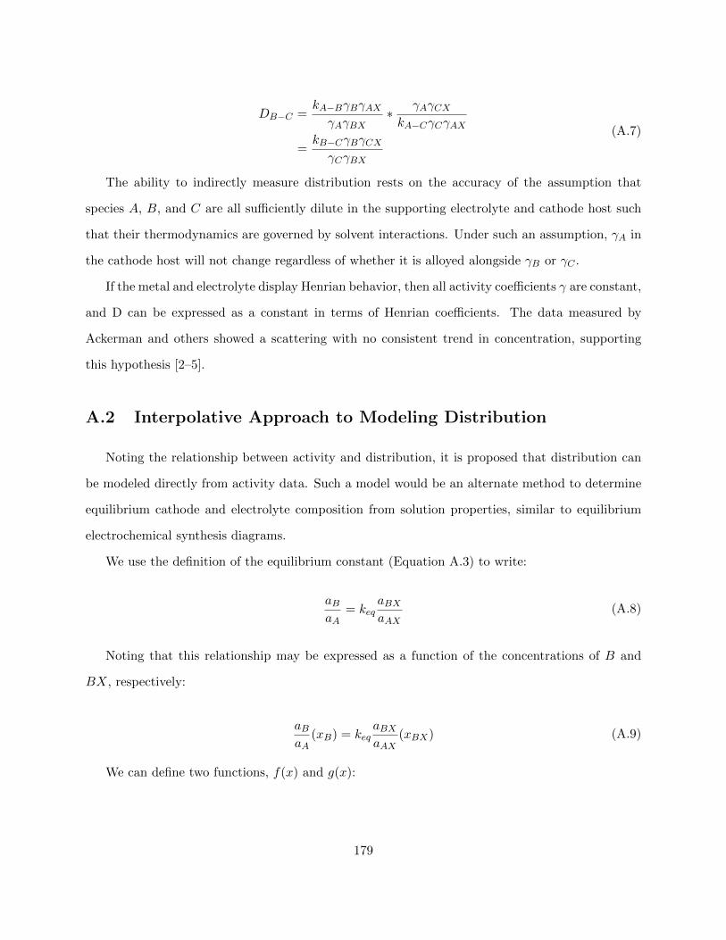
DB−C =kA−BγBγAXγAγBX
∗ γAγCXkA−CγCγAX
=kB−CγBγCXγCγBX
(A.7)
The ability to indirectly measure distribution rests on the accuracy of the assumption that
species A, B, and C are all sufficiently dilute in the supporting electrolyte and cathode host such
that their thermodynamics are governed by solvent interactions. Under such an assumption, γA in
the cathode host will not change regardless of whether it is alloyed alongside γB or γC .
If the metal and electrolyte display Henrian behavior, then all activity coefficients γ are constant,
and D can be expressed as a constant in terms of Henrian coefficients. The data measured by
Ackerman and others showed a scattering with no consistent trend in concentration, supporting
this hypothesis [2–5].
A.2 Interpolative Approach to Modeling Distribution
Noting the relationship between activity and distribution, it is proposed that distribution can
be modeled directly from activity data. Such a model would be an alternate method to determine
equilibrium cathode and electrolyte composition from solution properties, similar to equilibrium
electrochemical synthesis diagrams.
We use the definition of the equilibrium constant (Equation A.3) to write:
aBaA
= keqaBXaAX
(A.8)
Noting that this relationship may be expressed as a function of the concentrations of B and
BX, respectively:
aBaA
(xB) = keqaBXaAX
(xBX) (A.9)
We can define two functions, f(x) and g(x):
179

0.0 0.2 0.4 0.6 0.8 1.0
0.8
0.85
0.9
0.95
1
31
44
57
70
83
xBX
xB D
Figure A.1: Plot showing the relationship between the concentration of B in the cathode and BXin the electrolyte, as well as the calculated distribution for each concentration. Both metal and elec-trolyte are assumed to follow the regular solution model, with T=1250K, Zmetal=10, Zelectrolyte=10,Ωmetal=300, Ωelectrolyte=-300.
f(xB) = keqg(xBX) (A.10)
This allows for the expression of the concentration xB in terms of xBX :
(xB) = f−1(keqg(xBX)) (A.11)
This relationship can be solved analytically if a solution model, such as the regular solution
model, is available. It can also be solved graphically by interpolating the activity curves for both
B and BX. Figure A.1 shows the link between electrolyte composition and cathode composition,
as well as the distribution at each composition, calculated with Equation A.11.
180
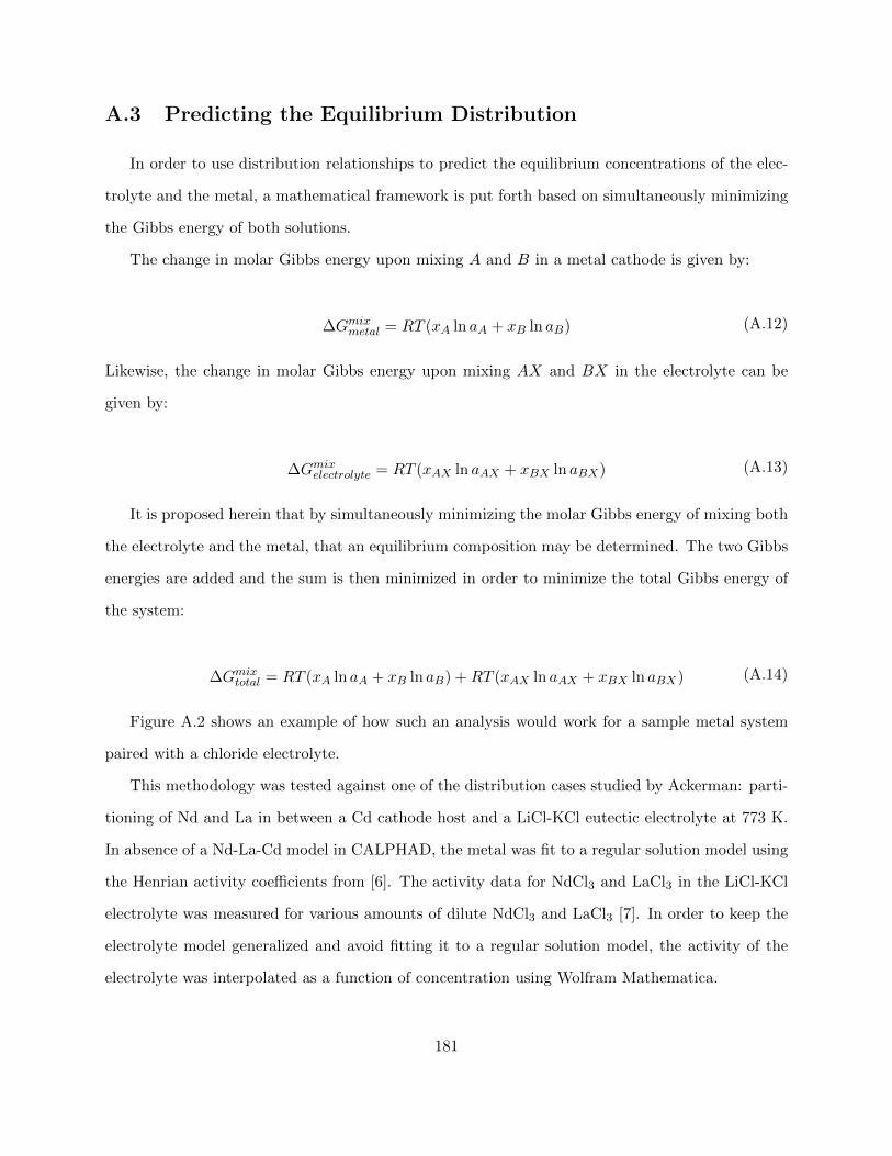
A.3 Predicting the Equilibrium Distribution
In order to use distribution relationships to predict the equilibrium concentrations of the elec-
trolyte and the metal, a mathematical framework is put forth based on simultaneously minimizing
the Gibbs energy of both solutions.
The change in molar Gibbs energy upon mixing A and B in a metal cathode is given by:
∆Gmixmetal = RT (xA ln aA + xB ln aB) (A.12)
Likewise, the change in molar Gibbs energy upon mixing AX and BX in the electrolyte can be
given by:
∆Gmixelectrolyte = RT (xAX ln aAX + xBX ln aBX) (A.13)
It is proposed herein that by simultaneously minimizing the molar Gibbs energy of mixing both
the electrolyte and the metal, that an equilibrium composition may be determined. The two Gibbs
energies are added and the sum is then minimized in order to minimize the total Gibbs energy of
the system:
∆Gmixtotal = RT (xA ln aA + xB ln aB) +RT (xAX ln aAX + xBX ln aBX) (A.14)
Figure A.2 shows an example of how such an analysis would work for a sample metal system
paired with a chloride electrolyte.
This methodology was tested against one of the distribution cases studied by Ackerman: parti-
tioning of Nd and La in between a Cd cathode host and a LiCl-KCl eutectic electrolyte at 773 K.
In absence of a Nd-La-Cd model in CALPHAD, the metal was fit to a regular solution model using
the Henrian activity coefficients from [6]. The activity data for NdCl3 and LaCl3 in the LiCl-KCl
electrolyte was measured for various amounts of dilute NdCl3 and LaCl3 [7]. In order to keep the
electrolyte model generalized and avoid fitting it to a regular solution model, the activity of the
electrolyte was interpolated as a function of concentration using Wolfram Mathematica.
181
0 0.2 0.4 0.6 0.8 1
-140
-100
-60
-20
0 0.2 0.4 0.6 0.8 1
-220
-215
-210
-205
ΔGmix(electrolyte)
ΔGmix(metal)
ΔGm
ix(e
lect
roly
te/m
etal
)/kJ
AAX
xBxBX
BBX
AX xBX BX
ΔG
mix
(tota
l)/kJ
a)
b)
Figure A.2: a) ∆Gmix for sample metallic and electrolyte systems. b) Sum of ∆Gmixmetal and∆Gmixelectrolyte.
182

LaCl3 xNdCl3 NdCl30.2 0.4 0.6 0.8 1.00
1
2
3
4
5
6
Dis
tribu
tion
Figure A.3: Distribution of La and Nd between a LiCl-KCl electrolyte and a Cd cathode. s: :modeled distribution from thermodynamic data and summed Gibbs energies of mixing La-Nd andLaCl3-NdCl3. : experimentally determined distribution. Data from [2, 3].
.
In this way, Gibbs energy curves of both the La-Nd and LaCl3-NdCl3 pseudobinaries in Cd and
LiCl-KCl, respectively, were generated. The sum of both of these curves were minimized, and the
concentration of NdCl3 at this minimum energy was taken as the equilibrium concentration. This
value was then used to find D, the distribution parameter, through equations A.2 and A.11. Fig-
ure A.3 shows the value of the calculated distribution compared to the experimentally determined
values from Ackerman [2, 3].
These preliminary results are encouraging. The modeled result is within the range of error for
the experimental values, both in concentration of NdCl3 as well as in distribution.
183
A.4 Perspectives on Further Model Development
The expansion of the distribution model proposed above shows promise for correctly predicting
electrochemical outcomes. However, it is critical to note that further study is necessary to refine
the model and correctly determine its limitations. Additional case studies should be tested to verify
this approach. From the preliminary study, specific shortcomings of the model became apparent:
these shortcomings must be addressed before further development and implementation can occur.
A.4.1 Boundary Conditions
One of the strengths of this model is the ability to work independently of CALPHAD models
and generate Gibbs energy curves directly from experimental data. To facilitate this, the Gibbs
energies of mixing are re-framed along the pseudobinary of the species in question. In the La-Nd
case, for example, the concentrations of LaCl3 and NdCl3 was constrained at 0-2.64 mol% in the
LiCl-KCl eutectic. The concentrations of La and Nd were also limited to the same amount in the
Cd cathode. 2.64 mol% was the highest available concentration for which there was activity data.
Such a cap kept the development of an expression for activity in the interpolation range, rather
than in the extrapolation range.
However, if the data range was narrowed even further, to 2 mol% electroactive species in the
supporting electrolyte, then the modeled distribution value was observed to change. Distribution
shifted from its original value of 1.04 (Figure A.3) to 1.6. The predicted concentration of NdCl3
also shifted, albeit by a smaller amount: from 81 mol% NdCl3 to 80 mol%. Similar shifts were also
noticed with changes in interpolation step size.
Although the results of this shift were still within the range of experimental error, the shift
itself causes concern. It suggests that the initial boundary conditions of the model are ill-defined.
One possible explanation could be issues with the interpolating functions used. The expression
developed for the activities of LaCl3 and NdCl3 were used in Equation A.11 to calculate distribution
at each composition. Errors in defining activity between data points by using interpolation would
propogate through the inverse function calculations. Such errors would also impact calculations of
184

the minima or common tangents for Gibbs energy curves, and would be most pronounced at the
edges of the interpolation regime (minimum or maximum concentration).
A second explanation could be that imposing such a boundary condition on the concentration of
metal and electrolyte is not possible. The equilibrium distribution of two species between the metal
and electrolyte may not exist within the pre-defined boundaries (i.e. the equilibrium electrolyte or
metal composition may be greater than 2.64 mol%). For this reason, the consequences of adding two
Gibbs energy curves defined along a molar pseudobinary is not quite clear. Further mathematical
and thermodynamic analyses are necessary in order to understand the limitations of this method,
and if the entire concentration regime must be defined before modeling (similarly to how equilibrium
electrochemical synthesis diagrams are modeled).
The small concentration regimes studied are also a cause for concern. The distribution studies
referenced focused on solutions that were dilute both in the Cd cathode as well as the chloride
electrolyte. If the changes in modeled distribution as a function of boundary condition are in
fact due to propogated errors from interpolation, then the magnitude of these errors would be
exaggerated as the concentration regimes studied tend towards dilution. For example, if the La-Nd
species were concentrated at 90 mol% of the total solution, then model deviations by 0.5mol% would
mean roughly 0.6% error. If La-Nd were dilute at 2.5 mol% of the total solution, then the same
amount of deviation would cause a 20% error. A comparison of model tolerance for concentrated
and dilute cases is therefore necessary.
A.4.2 Extension to More Complex Systems
Once the boundary conditions of the model have been appropriately defined and possible sources
for error are clarified, the next important step in model development is testing it on other systems
and case studies. Validation in other electrolytes, such as fluorides or oxides, should be considered.
Special attention should be paid to ensure accurate modeling of phase phenomena, such as phase
separation or compound formation.
In the distribution experiments cited above, as well as in the model derived in this appendix,
the case studies focused on instances where one mole of metal produced one mole of electrolyte:
185

La to LaCl3 and Nd to NdCl3. This stoichiometry is fortuitous because it not only allows the
Gibbs energies of mixing to be defined on the same molar basis, but also the exchange between La
and Nd does not result in production of additional species, such as Cl2. In order to accommodate
electrolytes with other stoichiometries, the derivation should be generalized and the model should
be rigorously tested using these cases.
A.5 Final Thoughts
Distribution modeling represents a complement to the electrochemical synthesis diagram mod-
eling discussed in this thesis. Both models share significant similarities, and both aim to link the
properties of two solutions (electrolyte and metal) by minimizing the Gibbs energy of these solu-
tions. Synthesis diagrams are limited by their dependence on a complete solution model for the
cathode. As such, they cannot be used when the properties of the cathode alloy are unknown.
However, no activity data is required for the electrolyte.
In contrast, distribution models use limited experimental data for both solutions. Thus, while
they rely on the availability of absolute activity measurements in the electrolyte, significantly less
information is needed on the metal side. Early results of this model are encouraging, but they have
only been applied to one system and the limitations are not entirely clear yet. Further investigation
is needed before distribution modeling can be more broadly applied to understanding the behavior
of electrochemical solutions.
186
Bibliography
[1] G. Kaptay. “The conversion of phase diagrams of solid solution type into electrochemical
synthesis diagrams for binary metallic systems on inert cathodes”. In: Electrochimica Acta
60 (Jan. 2012), pp. 401–409. issn: 00134686. doi: 10.1016/j.electacta.2011.11.077.
[2] John P Ackerman. “Chemical Basis for Pyrochemical Reprocessing of Nuclear Fuel”. In: Ind.
Eng. Chem. Res. 30.1 (1991), pp. 141–5. url: https://pubs.acs.org/sharingguidelines.
[3] John P. Ackerman and Jack L. Settle. “Distribution of plutonium, americium, and several rare
earth fission product elements between liquid cadmium and LiCl-KCl eutectic”. In: Journal
of Alloys and Compounds 199 (Sept. 1993), pp. 77–84. issn: 09258388. doi: 10.1016/0925-
8388(93)90430-U.
[4] M Kurata et al. “Distribution behavior of uranium, neptunium, rare-earth elements (Y, La,
Ce, Nd, Sm, Eu, Gd) and alkaline-earth metals (Sr,Ba) between molten LiC1-KC1 eutectic
salt and liquid cadmium or bismuth”. In: Journal of Nuclear Materials 227 (1995), pp. 110–
121.
[5] Y Sakamura et al. “Distribution behavior of plutonium and americium in LiCl–KCl eutec-
tic/liquid cadmium systems”. In: Journal of Alloys and Compounds 321 (May 2001), pp. 76–
83. issn: 09258388. doi: 10.1016/S0925-8388(01)00973-2.
[6] Masaki Kurata, Yoshiharu Sakamura, and Tsuneo Matsui. “Thermodynamic quantities of
actinides and rare earth elements in liquid bismuth and cadmium”. In: Journal of Alloys and
Compounds 234.1 (1996), pp. 83–92. issn: 09258388. doi: 10.1016/0925-8388(95)01960-X.
187

[7] Jinsuo Zhang et al. Rare Earth Electrochemical Property Measurements and Phase Diagram
Development in a Complex Molten Salt Mixture for Molten Salt Recycle. Tech. rep. US De-
partment of Energy, 2018, p. 193. url: https://www.osti.gov/servlets/purl/1432448.
188
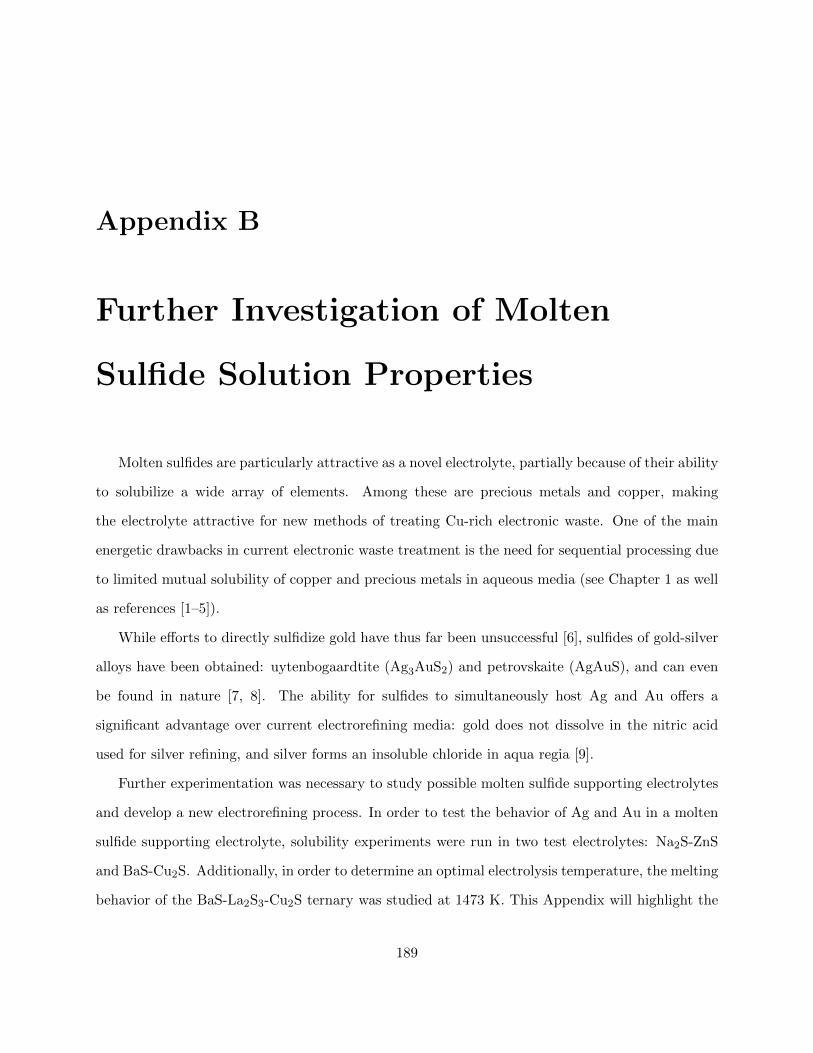
Appendix B
Further Investigation of Molten
Sulfide Solution Properties
Molten sulfides are particularly attractive as a novel electrolyte, partially because of their ability
to solubilize a wide array of elements. Among these are precious metals and copper, making
the electrolyte attractive for new methods of treating Cu-rich electronic waste. One of the main
energetic drawbacks in current electronic waste treatment is the need for sequential processing due
to limited mutual solubility of copper and precious metals in aqueous media (see Chapter 1 as well
as references [1–5]).
While efforts to directly sulfidize gold have thus far been unsuccessful [6], sulfides of gold-silver
alloys have been obtained: uytenbogaardtite (Ag3AuS2) and petrovskaite (AgAuS), and can even
be found in nature [7, 8]. The ability for sulfides to simultaneously host Ag and Au offers a
significant advantage over current electrorefining media: gold does not dissolve in the nitric acid
used for silver refining, and silver forms an insoluble chloride in aqua regia [9].
Further experimentation was necessary to study possible molten sulfide supporting electrolytes
and develop a new electrorefining process. In order to test the behavior of Ag and Au in a molten
sulfide supporting electrolyte, solubility experiments were run in two test electrolytes: Na2S-ZnS
and BaS-Cu2S. Additionally, in order to determine an optimal electrolysis temperature, the melting
behavior of the BaS-La2S3-Cu2S ternary was studied at 1473 K. This Appendix will highlight the
189
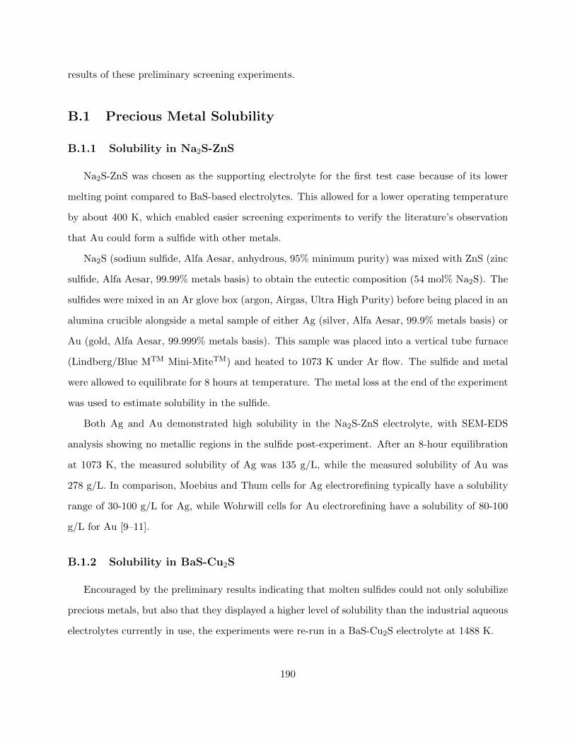
results of these preliminary screening experiments.
B.1 Precious Metal Solubility
B.1.1 Solubility in Na2S-ZnS
Na2S-ZnS was chosen as the supporting electrolyte for the first test case because of its lower
melting point compared to BaS-based electrolytes. This allowed for a lower operating temperature
by about 400 K, which enabled easier screening experiments to verify the literature’s observation
that Au could form a sulfide with other metals.
Na2S (sodium sulfide, Alfa Aesar, anhydrous, 95% minimum purity) was mixed with ZnS (zinc
sulfide, Alfa Aesar, 99.99% metals basis) to obtain the eutectic composition (54 mol% Na2S). The
sulfides were mixed in an Ar glove box (argon, Airgas, Ultra High Purity) before being placed in an
alumina crucible alongside a metal sample of either Ag (silver, Alfa Aesar, 99.9% metals basis) or
Au (gold, Alfa Aesar, 99.999% metals basis). This sample was placed into a vertical tube furnace
(Lindberg/Blue MTM Mini-MiteTM) and heated to 1073 K under Ar flow. The sulfide and metal
were allowed to equilibrate for 8 hours at temperature. The metal loss at the end of the experiment
was used to estimate solubility in the sulfide.
Both Ag and Au demonstrated high solubility in the Na2S-ZnS electrolyte, with SEM-EDS
analysis showing no metallic regions in the sulfide post-experiment. After an 8-hour equilibration
at 1073 K, the measured solubility of Ag was 135 g/L, while the measured solubility of Au was
278 g/L. In comparison, Moebius and Thum cells for Ag electrorefining typically have a solubility
range of 30-100 g/L for Ag, while Wohrwill cells for Au electrorefining have a solubility of 80-100
g/L for Au [9–11].
B.1.2 Solubility in BaS-Cu2S
Encouraged by the preliminary results indicating that molten sulfides could not only solubilize
precious metals, but also that they displayed a higher level of solubility than the industrial aqueous
electrolytes currently in use, the experiments were re-run in a BaS-Cu2S electrolyte at 1488 K.
190
Barium sulfide (BaS, Alfa Aesar, 99.7% metals basis) and copper sulfide (Cu2S, Strem Chemi-
cals, 99.5% metals basis) were mixed together in an Ar glove box (argon, Airgas, Ultra High Purity)
and pre-melted in a graphite crucible (C, The Graphite Store, Grade EC-16) under Ar flow before
being placed in a graphite crucible alongside a metal sample of either Ag (silver, Alfa Aesar, 99.9%
metals basis) or Au (gold, Alfa Aesar, 99.999% metals basis). Both Ag and Au were pre-melted in
an arc melter (Compact Arc Melter MAM-1, Edmund Buhler) under Ar atmosphere in the presence
of a zirconium oxygen getter (Zr, Alfa Aesar, 99.5% metals basis (excluding Hf), Hf 3%) in order
to remove any residual oxygen from the metal. The graphite crucible was loaded into a vertical
tube furnace (Mellen, SS15R-2.50X6V- 1Z) and heated to 1488 K under Ar flow. After an 8-hour
hold at temperature, the sample was quenched by lowering from the central, heated area of the
tube to the lower, colder end of the tube (Chapter 5). Post-experiment, the metal and sulfide were
separated and weighed. Solubility was estimated by metal weight loss and the sulfide was crushed
into a powder, mounted in epoxy, polished to 2000 grit, and examined under SEM-EDS to ensure
there were no metallic regions present.
Upon cooling, it was found that the BaS-Cu2S electrolyte separated into BaS-rich and Cu2S-rich
regions. Figure B.1 shows the typical microstructure of the electrolyte after equilibration with Ag.
Ag was found to segregate to the Cu-rich phase, with an overall measured solubility of 53 g/L.
Figure B.2 shows the typical microstructure observed after Au solubility experiments. In con-
trast to Ag, Au did not segregate to the Cu-rich phase, but rather formed a phase of its own
with moderate amounts of Ba, Cu, and S. The solubility of Au in the BaS-Cu2S electrolyte was
relatively lower than that measured in Na2S-ZnS: 26 g/L after 8 hours. However, it is likely that
equilibrium solubility was not achieved in 8 hours in this electrolyte. A follow-up experiment held
at temperature for 24 hours resulted in total dissolution of the gold sample. This indicates that
Au has a solubility in the BaS-Cu2S electrolyte greater than 160 g/L, a value more similar to that
observed in Na2S-ZnS.
While Ag appeared to dissolve in the Cu-rich phase of the electrolyte, in which Ag ions could
have possibly substituted for Cu to form a BaS-Cu2S-Ag2S phase, Au showed a different behavior.
It is possible that the Au-rich sulfide phase was an entirely new compound, Au4Cu3Ba6S6, which
191

primaryphase
secondary phase
primaryphase
Figure B.1: SEM image of quenched sulfide from Ag solubility experiments in BaS-Cu2S electrolyte.Primary phase composition (mol%): 37% S, 29% Ba, 29% Cu, 5% Ag. Secondary phase composition(mol%): 39 % S, 59% Ba, 2% Cu.
.
192

primary phase
secondary phase
primary phase
tertiary phasesecondary
phase
Figure B.2: SEM image of quenched sulfide from Au solubility experiments in BaS-Cu2S electrolyte.Primary phase composition (mol%): 34% S, 32% Ba, 33% Cu. Secondary phase composition(mol%): 37% S, 60% Ba, 2% Cu. Tertiary phase composition (mol %): 33% S, 29% Ba, 17% Cu,21% Au
.
193

would be in keeping with current observations about Au-sulfides. It has been observed that while
Au2S is generally unstable, Au combined with other metals form more stable sulfides [6–8].
B.2 Isothermal Study of BaS-La2S3-Cu2S Ternary
Research on Cu electrolysis from BaS-Cu2S electrolyte indicated that addition of a third elec-
trolyte, La2S3 may improve the properties of the supporting electrolyte, promoting ionic conduc-
tivity and lowering the vapor pressure [12]. In order to understand the melting behavior of this
new electrolyte, an isothermal study of the material near electrolysis temperature (1473 K) was
run.
Sulfide at various concentrations of barium sulfide (BaS, Alfa Aesar, 99.7% metals basis), cop-
per sulfide (Cu2S, Strem Chemicals, 99.5% metals basis), and lanthanum sulfide (La2S3, Strem
Chemicals, 99.9% metals basis) were mixed in an Ar glove box and loaded into a specially designed
graphite crucible (C, The Graphite Store, Grade EC-16) that could accommodate 0.5 g of each
composition. Figure B.3a details the tested concentrations along the ternary, and Figure B.3b
shows the design of the crucible used. A custom-designed cap for the crucible that fit tightly into
each sample well was used to limit volatilization. Small screws that fit into the four drill-holes in
each arm of the cross further tightened the seal. The setup was loaded into a vertical tube furnace
(Carbolite, model PVT 18/100/350) and temperature was monitored with a “type C” thermocouple
using an Omega data aquisition system (Omega Engineering, Model QMB-DAQ-55). The furnace
was allowed to heat up to 1473 K before being held at temperature for 4 hours under a flow of Ar
to ensure an inert atmosphere.
After the 4-hour hold, the the crucible was slow-cooled to room temperature and then removed
from the furnace. It was kept in the Ar glovebox until it was ready to be opened. Upon opening,
the resulting compositions were photographed and moved to storage vials. These vials were then
transferred back to the glovebox, where the final contents were weighed. Visual inspection was
used to determine if the samples were “entirely melted”, “unmelted”, or “somewhat melted”.
(Figure B.3c). This information was used to determine a preliminary phase diagram by separating
194

a) b)
c)
Figure B.3: a) BaS-La2S-Cu2S ternary concentrations tested during isothermal experiment. b)custom-designed graphite crucible showing sample wells and drill holes. c) example of typical“melted”, “unmelted”, and “somewhat melted” samples post-experiment.
195
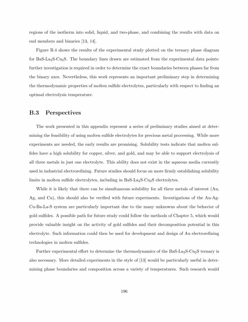
regions of the isotherm into solid, liquid, and two-phase, and combining the results with data on
end members and binaries [13, 14].
Figure B.4 shows the results of the experimental study plotted on the ternary phase diagram
for BaS-La2S-Cu2S. The boundary lines drawn are estimated from the experimental data points:
further investigation is required in order to determine the exact boundaries between phases far from
the binary axes. Nevertheless, this work represents an important preliminary step in determining
the thermodynamic properties of molten sulfide electrolytes, particularly with respect to finding an
optimal electrolysis temperature.
B.3 Perspectives
The work presented in this appendix represent a series of preliminary studies aimed at deter-
mining the feasibility of using molten sulfide electrolytes for precious metal processing. While more
experiments are needed, the early results are promising. Solubility tests indicate that molten sul-
fides have a high solubility for copper, silver, and gold, and may be able to support electrolysis of
all three metals in just one electrolyte. This ability does not exist in the aqueous media currently
used in industrial electrorefining. Future studies should focus on more firmly establishing solubility
limits in molten sulfide electrolytes, including in BaS-La2S-Cu2S electrolytes.
While it is likely that there can be simultaneous solubility for all three metals of interest (Au,
Ag, and Cu), this should also be verified with future experiments. Investigations of the Au-Ag-
Cu-Ba-La-S system are particularly important due to the many unknowns about the behavior of
gold sulfides. A possible path for future study could follow the methods of Chapter 5, which would
provide valuable insight on the activity of gold sulfides and their decomposition potential in this
electrolyte. Such information could then be used for development and design of Au electrorefining
technologies in molten sulfides.
Further experimental effort to determine the thermodynamics of the BaS-La2S-Cu2S ternary is
also necessary. More detailed experiments in the style of [13] would be particularly useful in deter-
mining phase boundaries and composition across a variety of temperatures. Such research would
196

Figure B.4: Estimated isothermal projection of BaS-La2S-Cu2S system at 1473 K based on observedmelting behavior.
197

advise electrochemists on the best temperature and composition to ensure that their electrolyte is
a stable liquid, ideally with a low vapor pressure. Future isothermal studies are also recommended
to focus on the areas of the ternary where liquid and solid phases are predicted to be in equilibrium,
in order to further refine the estimated ternary projection.
198
Bibliography
[1] S.A. Mastyugin and S.S. Naboichenko. “Processing of Copper-Electrolyte Slimes: Evolution
of Technology”. In: Russian Journal of Non-Ferrous Metals 53.5 (2012), pp. 367–374. doi:
10.3103/S1067821212050070.
[2] J Hait, R K Jana, and S K Sanyal. “Processing of copper electrorefining anode slime:
a review”. In: Trans. Inst. Min. Metall. C. 118.4 (2009), pp. 240–252. doi: 10 . 1179 /
174328509X431463.
[3] T Chen and J E Dutrizac. “Mineralogical overview of the behavior of gold in conventional
copper electrorefinery anode slimes processing circuits”. In: J E Minerals & Metallurgical
Processing Aug 25.3 (2008), pp. 156–164.
[4] Ailiang Chen et al. “Recovery of Silver and Gold from Copper Anode Slimes”. In: JOM
Journal of the Minerals, Metals and Materials Society 67.2 (2015), pp. 493–502. doi: 10.
1007/s11837-014-1114-9.
[5] C Segawa and T Kusakabe. “Current Operations in SMM’s Slime Treatment”. In: TMS
Extraction and Processing Division. Anaheim, Ca, 1996. url: http://www.isasmelt.com/
EN/Publications/TechnicalPapersBBOC/SMM’s%20Slime%20Treatment.pdf.
[6] Mark D. Barton. “The Ag-Au-S System”. In: Economic Geology 75 (1980), pp. 303–316. issn:
0361-0128. doi: 10.2113/gsecongeo.75.2.303.
[7] G.A. Pal’yanova and N.E. Savva. “Some Sulfides of Gold and Silver: Composition, Mineral
mineral Assemblage, and Conditions of Formation”. In: Theoretical Foundations of Chemical
Engineering 42.5 (2008), pp. 749–761. doi: 10.1134/S0040579508050485.
199
[8] Galina Palyanova, Nick Karmanov, and Natalie Savva. “Sulfidation of native gold”. In: Amer-
ican Mineralogist 99.5-6 (2014), pp. 1095–1103. doi: 10.2138/am.2014.4677.
[9] K G Fisher. “Refining of Gold At the Rand Refinery”. In: Extractive Metallurgy of Gold in
South Africa. Ed. by G.G. Stanley. Johannesburg: South African Institution of Mining and
Metallurgy, 1987. Chap. 10, pp. 615–653. isbn: 978-1468484274.
[10] C. L. Mantell. Electrochemical Engineering. Fourth. New York, NY: McGraw-Hill, 1960. isbn:
0-07-040028-8.
[11] Umicore AG & Co. KG. Precious Materials Handbook. 1st ed. Hanau-Wolfgang: Umicore AG
& Co, KG, 2012. isbn: 978-3-8343-3259-2.
[12] Sulata K. Sahu, Brian Chmielowiec, and Antoine Allanore. “Electrolytic Extraction of Cop-
per, Molybdenum and Rhenium from Molten Sulfide Electrolyte”. In: Electrochimica Acta
243 (2017), pp. 382–389. issn: 00134686. doi: 10.1016/j.electacta.2017.04.071.
[13] Caspar Stinn et al. “Experimentally Determined Phase Diagram for the Barium Sulfide-
Copper(I) Sulfide System Above 873 K (600 °C)”. In: Metallurgical and Materials Trans-
actions B 48.6 (2017), pp. 2922–2929. doi: 10.1007/s11663-017-1107-5. url: https:
//link.springer.com/content/pdf/10.1007/s11663-017-1107-5.pdf.
[14] N V Sikerina et al. “Phase equilibria in the BaS-Cu2S-Gd2S3 system”. In: Zh. Neorg. Khim.
52.Copyright (C) 2012 American Chemical Society (ACS). All Rights Reserved. (2007),
pp. 2099–2103.
200