arX

iv:h

ep-t

h/96

0515

4v3

24

May

199

6

CERN-TH/96-133NSF-ITP-95-162OSU-M-96-6hep-th/9605154

New Higgs Transitions between Dual N=2 String Models

Per Berglund

Theory Division, CERN

CH-1211 Geneva 23, Switzerland

Sheldon Katz

Department of Mathematics

Oklahoma State University

Stillwater, OK 74078, USA

Albrecht Klemm

Department of Mathematics, Harvard University

Cambridge MA 02138, USA

Peter Mayr

Theory Division, CERN

CH-1211 Geneva 23, Switzerland

We describe a new kind of transition between topologically distinct N = 2 type IICalabi–Yau vacua through points with enhanced non-abelian gauge symmetriestogether with fundamental charged matter hyper multiplets. We connect theappearance of matter to the local geometry of the singularity and discuss therelation between the instanton numbers of the Calabi–Yau manifolds taking partin the transition. In a dual heterotic string theory on K3 × T 2 the processcorresponds to Higgsing a semi-classical gauge group or equivalently to a variationof the gauge bundle. In special cases the situation reduces to simple conifoldtransitions in the Coulomb phase of the non-abelian gauge symmetries.

CERN-TH/96-133

5/96

Email: berglund@nxth04.cern.ch, katz@math.okstate.edu, klemm@abel.math.harvard.edu,

mayr@surya11.cern.ch

1. Introduction

During the last few years there has been a great deal of progress in the understanding

of non-perturbative phenomena in supersymmetric field theories as well as in various string

theories [1]. In particular the idea of duality has proven to be crucial. The basic point

here is that one underlying theory might have several descriptions in terms of physical

variables. In the current setting these ideas originated in the work by Seiberg and Witten

in the context of N = 2 supersymmetric Yang-Mills theory [2]. For all gauge groups

the global prepotential can be derived from the periods of a suitable auxiliary Riemann-

surface [3]. Combining the properties of N = 2 gauge theories with the conjectured duality

between N = 4 string theories in four dimensions [4] it was suggested that also N = 2

string theories in four dimensions have a duality structure; the heterotic string theory

compactified on K3 × T 2 and the type II theory compactified on a Calabi-Yau manifold,

could be dual to each other after including non-perturbative states [5][6].

In [5] concrete pairs of dual N = 2 theories were constructed in which non-perturbative

properties of the heterotic string can be investigated exactly. The key idea is the absence

of neutral couplings between vector multiplets and hyper multiplets in N = 2 theories [7].

As the heterotic dilaton sits in a vector multiplet the vector multiplet moduli space can

receive space-time perturbative and non-perturbative corrections. Under N = 2 string-

string-duality it is identified with the vector multiplet moduli space of the Type IIA string,

which corresponds to the Kahler moduli space of the compactified Calabi-Yau manifold.

The latter has to have Hodge numbers h11 = Nv and h21 = Nh − 1, where Nv, Nh are the

number of vector and hyper multiplets and the −1 corresponds to the the dilaton of the

type II string. (Note however, that the rank of the gauge group is Nv+1 as the graviphoton

contributes a U(1)-factor.) As the Type IIA dilaton is in a hyper multiplet the vector mul-

tiplet moduli space is exact at tree level and so is not corrected by space-time instantons.

It is, however, corrected by worldsheet instantons. By mirror symmetry we can identify it

with the hyper multiplet moduli space of the Type IIB theory on the mirror Calabi-Yau

manifold, which receives neither world-sheet nor space-time corrections. The upshot is

that the exact non-perturbative vector multiplet moduli space of the heterotic string is

modelled by the complex structure moduli space of a specific Calabi-Yau manifold 1. In

this sense the complex moduli space of Calabi-Yau manifold replaces the complex moduli

space of the auxiliary Riemann surface, which one had in the N = 2 Yang-Mills field theory

case.

Following the initial work [5][6] a number of consistency checks have been made further

establishing the conjectured type II/heterotic string duality; comparison of the perturba-

tive region of the potentials [9] of the heterotic couplings (gauge and gravitational) with

1 Similarly, the structure of the non-perturbative hyper moduli space of the type IIA theory,

which is a quaternionic manifold [8] can be investigated via the heterotic string.

1

that of the dual type IIA vacuum [5], [10], as well as non-perturbative consistency checks

in the point-particle limit [11].

Furthermore, and what will be the focus of this paper, aspects of the perturbative

enhancements of the gauge symmetry can be studied by considering the Picard lattice

of the generic K3-fiber [12]. Using the Higgs mechanism as a way of lowering the rank

of the gauge group and thus finding a way in which the various moduli spaces can be

connected2[13], chains of such transitions have been studied extensively [5][14] [15].

Here we will focus on a particular chain and investigate in detail the transition from

the point of view of the local geometry as well as in terms of the the worldsheet instanton

sums in the type IIA theory. In particular, we will not only be able to identify the en-

hanced perturbative gauge symmetry but also the matter representations. The geometrical

transition is of a slightly generalized type compared to the conifold transitions on one hand

and the strong coupling transitions on the other hand. In addition to having N-1 divisors

being contracted to a singular curve C, of genus zero, giving rise to an SU(N) theory with

no adjoint hyper multiplets [16], there are singular fibers, which when contracted to C give

rise to massless hyper multiplets in the fundamental representation. The general structure

of these transitions is discussed in section 2. We then turn to a specific set of models in

section 3. This chain of Calabi-Yau manifolds can be viewed as K3 fibrations over P1 as

well as elliptic fibrations over the Hirzebruch surface F2. Finally, we end with conclusions

and discussions in section 4.

2. Structure of the extremal transitions

2.1. Physical spectrum and flat directions

It will be useful to consider the purely field theoretic problem of which massless

particles will appear in the moduli space. At a generic point in the moduli space of

vacuum expectation values of the scalar component of the vector multiplet, the gauge

symmetry is U(1)N−1. By a suitable gauge transformation we can then write the above

scalar in the diagonal form diag(φ1, ..., φN), where∑N

i=1 φi = 0 and φi 6= φj , for all i, j.

Clearly, all the matter fields are massive with masses proportional to φi. If we now set

φi = 0, i = 1, ..., N − 1, the gauge symmetry is enhanced to SU(N) and only matter fields

charged with respect to the SU(N) become massless. Let us for simplicity assume that

there are M fields which all transform in the fundamental representation. Because of the

tracelessness condition there exists a surface for which one can have SU(N − 1) × U(1),

2 This so called Higgs-branch has to be distinguished from the Higgs breaking mechanism into

the Coulomb-branch by vector multiplets, in which the gauge bosons become massive as short

vector multiplets under spontaneous generation of central charge, as in the Seiberg-Witten theory.

2

with φi = φj 6= 0, i, j = 1, ..., N −1 but without massless charged matter. If we reduce the

symmetry enhancement one step further there is however room for massless matter in the

fundamental of SU(N − 2); e.g. choose φi = 0, i = 1, ..., N − 2 and φN−1 = −φN 6= 0. In

general one will have several SU(kj); however, only the one for which φi = 0, i = 1, ..., kj

will have M massless matter multiplets. In particular, there exists a codimension one

surface in which only e.g. φ1 = 0, such that there is no gauge enhancement. However,

because of φ1 = 0 we will have M massless singlets. It is very gratifying that, as will now

be seen, the Calabi-Yau moduli space exactly reproduces this kind of behaviour.

2.2. Local geometry of the Calabi–Yau singularity

During the recent developments it has become clear that the physical singularities

associated to massless solitonic BPS states are essentially encoded in the geometry of

the singularity of the compactified manifold. The role played by the geometry can be

understood from the interpretation of the massless states as solitonic p-branes wrapped

around the vanishing cycles of the singularity; the gauge and Lorentz quantum numbers

depend then on some characteristic properties of the homology cycles, in particular their

dimension, topology and intersection numbers [16].

The simplest case (in the type IIB picture) is that of a vanishing three-cycle leading to

a massless hyper multiplet, the case considered originally by Strominger [17]. On the other

hand, if the three-cycle shrinks to a curve, rather than to a point, one obtains enhanced

gauge symmetries, as has been argued in [18]. More precisely, if the local geometry is that of

an ALE space with AN singularity over a curve of genus g one obtains an enhanced SU(N+

1) gauge symmetry [19] together with g hyper multiplets in the adjoint representation [16].

The case g = 0 is exceptional in that the enhanced gauge symmetry is asymptotically free

and broken to its abelian factor due to strong coupling effects in the infrared; this case has

been considered in [11] [20].

Let us now assume that we have a collection of curves Ci with the transverse space that

of an ALE-manifold with ANitype singularity and consider further a point of intersection

between two of these curves [21]. The singularity structure of the transverse space has

been analyzed in detail in [22] in the context of elliptic fibrations with the following result:

if along the curves C1 and C2 the elliptic fiber is of Kodaira type IN1and IN2

respectively,

then above the point where C1 intersects C2 the elliptic fiber is of type type IN1+N2. Indeed

the examples we will consider are all ellipticly fibered Calabi–Yau manifolds. This allows

in particular for a simple interpretation in terms of 5-branes [18] [16]located at the points

where the fibration becomes singular. However this special structure is not necessary; the

general configuration is that of a collection of curves Ci with transverse ANisingularities

colliding in a set of M points over which the singularity structure jumps to ANi+Nj.

A simple D-brane arrangement based on a collection of Ni coinciding D-branes in-

tersecting a second collection of Nj coinciding D-branes has been given in [18]. In this

3

picture additional matter in the fundamental representation arises from open string states

with one end attached to the first and the other end to the second collection. There is a

special configuration in which one of the two collections consists of a single D-brane only,

say Nj = 1. In this case one expects a single non-abelian factor of SU(Ni) together with

matter in the fundamental representation.

This is the physical situation whose realization we will consider in the context of

Calabi–Yau compactifications. Specifically the case of SU(N + 1) gauge symmetry with

M fundamental matter multiplets arises from the following local data: there is a curve

C, which in our case will be a P 1, over which one has a bundle structure where the

generic fiber is a Hirzebruch-Jung tree of the resolution of the AN singularity, that is a

collection of P 1’s, Ei, i = 1..N with intersection matrix proportional to the Cartan matrix

of AN . In addition, above the M exceptional points, the singularity structure of the fiber

becomes AN+1 because one component of the fiber factorizes. More precisely out of the

N generic components N − 1 are toric divisors Di of the manifold Xi which are ruled

surfaces, while the N -th component, E is only birationally ruled, having M degenerate

fibers. The last component E is actually a conic bundle, which means that the fibers are

all plane conics [23]. These conics are smooth over a generic points of C while they split

into line pairs over the M exceptional points.

Let us describe now how the appearance of this structure will lead to geometrical

transitions between two Calabi–Yau manifolds Xi and Xi−1 (where i denotes the number

of NV = h11 of vector multiplets). First we can contract the N − 1 divisors together with

the M degenerate fibers of the conic bundle. According to our previous discussion, the

degenerate fibers contain a collection of N + 1 rational curves Ei with intersection matrix

of AN+1 which are all contracted. N of them are again associated to the Cartan subalgebra

of the gauge group while the additional one is related to the matter hyper multiplets; there

is a natural action of the AN Weyl group on this class which generates the components

of the fundamental representation. The gauge quantum numbers of the solitonic p-brane

states are determined by the reduction of the Cartan matrix of AN+1 to that of AN ; the

components of the matter fields arise naturally from wrappings of the cycles EN+1 − Ei,

i = 0, . . . , N ; however there is no independent modulus associated to the volume of EN+1

and correspondingly no additional vector multiplet3. This is expected from the fact that

the additional rational curves are isolated rather than being fibers of a ruled surface. After

the N surfaces have been contracted to the base the singularities can be simplified by a

deformation of the complex structure in such a way that the resulting singularity is the

contraction of N − 1 surfaces arising from Xi−1. This completes the transition from Xi to

Xi−1 at the enhanced symmetry points.

3 Here E0 is the homology cycle which fulfills the relation∑N

0Ei ∼ 0, reflecting the trace-

lessness condition of SU(N + 1), as discussed in the previous section.

4

Clearly, in the generic situation one will only contract subsets Si of the N −1 divisors

and/or the conic bundle with the M degenerate fibers. The result will depend on whether

a given subset Si contains E; if it does we will get from that factor an enhanced gauge

symmetry SU(ki + 1) together with M fundamental representations; however if it does

not, the result is that of a non-abelian gauge symmetry without matter, broken down to

the Cartan subalgebra by strong infrared dynamics . In fact if N > 1 we can contract only

E and the result is M representations of U(1), that is we are back to the familiar case of

the conifold singularity.

2.3. String moduli space

We turn now to a discussion of the string moduli spaces involved in the transition. The

latter is described by a motion in the vector multiplet moduli M space of the Calabi–Yau

manifold Xi to a locus where the vev of the scalar superpartner of a vector field vanishes

and then turning on vevs in the new flat directions of the Higgs branch corresponding

to a motion in the hyper multiplet moduli space of the Calabi–Yau manifold Xi−1; the

new Calabi-Yau manifold Xi−1 will therefore have fewer vector moduli while the number

of hyper moduli has increased; the associated change in the Hodge numbers h11 and h12

indicates that the two manifolds are of different topological type. There are two types of

natural coordinates on M, the algebraic coordinates zn and the special coordinates tn [24],

where the two are related by the mirrormaps zm(tn). We are interested in the relations

between these two types of coordinates on Mi and Mi−1.

N = 2 supersymmetry puts strong restrictions on these relations; in particular the

special geometry of the vector multiplets in the type IIA compactification constrains the

map between the two set of coordinates tin and ti−1n to be linear. Moreover we will find

simple relations between the Gromov–Witten invariants ni1,...,ih11on Mi and Mi−1, which

are defined in terms of the instanton corrected Yukawa couplings yabc as

yabc = y0abc +

∑

d1,...,dh11

nrd1,...,dh11

dadbdc

1 −∏h11

n=1 qdnn

h11∏

n=1

qdn

n

where the nrd1,...,dh11

is the virtual fundamental class of the moduli space of rational curves

of multidegree d1, . . . , dh11. Such a relation between the instanton numbers are of course

a special property of the type of singularity we consider and will not be present in other

types of transitions proceeding e.g. through non-canonical singularities.

In a way similar to that the special geometry of the vector moduli space restricts

the relations between the coordinates on MiV and Mi−1

V , the quaternionic structure of

the hyper moduli space of the type IIB theory compactified on the same pair of manifold

implies simple relations between the coordinates on the hyper multiplet moduli spaces, ξn.

They are related to the algebraic moduli zn by rational functions which in turn depend on

5

the special representation of the Calabi–Yau manifolds. In particular there are in general

different reflexive polyhedra describing the same Calabi–Yau space, however in different

algebraic coordinates related by rational transformations. It is convenient to choose a

preferred representation in which the relation between the algebraic moduli on Mi and

Mi−1 becomes particularly simple:

zi−1n =

∏

m

(zim)δn

m

From the definition of the algebraic coordinates this relation translates to linear relations

between the Mori vectors lin, li−1n , generating the dual of the Kahler cone. As a consequence

the smaller dual polyhedron ∆⋆i−1 is obtained from the larger one ∆⋆

i by omitting one of

the vertices4.

A new feature of the corresponding transition in the moduli space is that, rather than

beeing located at the zero locus of the principal discriminant or a restricted discriminant,

it can take place at one of the boundary divisors zn = 0. Such transitions where first

discussed in [25]; indeed this is the situation in the examples described in section 3 5.

Similar examples have been considered independently [27].

In the case when the Calabi–Yau is a K3 fibration [28], the vector moduli space of the

pair of Calabi–Yau manifolds can be mapped to that of the dual heterotic theory, the map

again being linear by the above mentioned argument. Of course this relation will depend

on the special compactification under consideration and will be discussed further in the

examples.

3. Global description of the Calabi-Yau spaces and examples

Given a four-dimensional N=2 heterotic vacuum it is far from trivial to find the dual

type IIA model. Although there has been some progress recently as far as understanding

the perturbative gauge structure on the type IIA side [12][29][26] there is still some guess

work to be done in terms of finding a Calabi-Yau manifold that will fit the bill. In fact,

recent work [30] indicates that there will in general exist more than one type IIA theory

which agrees with the perturbative heterotic vacuum under consideration. From now on,

we will assume that there is a set of models which to lowest order corresponds to their

counterparts in the heterotic chain, i.e. the number of vector multiplets and singlet hyper

multiplets agree, and the models are all K3-fibrations.

4 This kind of transition was originally studied in [25] and more recently in [26].5 A model with similar properties has been observed in [25].

6

3.1. A chain of connected Calabi–Yau manifolds

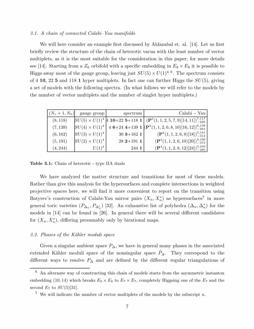
We will here consider an example first discussed by Aldazabal et. al. [14]. Let us first

briefly review the structure of the chain of heterotic vacua with the least number of vector

multiplets, as it is the most suitable for the consideration in this paper; for more details

see [14]. Starting from a Z6 orbifold with a specific embedding in E8 ×E8 it is possible to

Higgs away most of the gauge group, leaving just SU(5)×U(1)4 6. The spectrum consists

of 4 10, 22 5 and 118 1 hyper multiplets. In fact one can further Higgs the SU(5), giving

a set of models with the following spectra. (In what follows we will refer to the models by

the number of vector multiplets and the number of singlet hyper multiplets.)

(Nv + 1, Nh) gauge group spectrum Calabi − Yau

(8, 118) SU(5) × U(1)4 4 10+22 5+118 1 (P5(1, 1, 2, 5, 7, 9)[14, 11])7,117−220

(7, 139) SU(4) × U(1)4 4 6+24 4+139 1 (P5(1, 1, 2, 6, 8, 10)[16, 12])6,138−264

(6, 162) SU(3) × U(1)4 30 3+162 1 (P4(1, 1, 2, 6, 8)[18])5,161−312

(5, 191) SU(2) × U(1)4 28 2+191 1 (P4(1, 1, 2, 6, 10)[20])4,190−372

(4, 244) U(1)4 244 1 (P4(1, 1, 2, 8, 12)[24])3,243−480

Table 3.1: Chain of heterotic - type IIA duals

We have analyzed the matter structure and transitions for most of these models.

Rather than give this analysis for the hypersurfaces and complete intersections in weighted

projective spaces here, we will find it more convenient to report on the transition using

Batyrev’s construction of Calabi-Yau mirror pairs (Xn, X∗n) as hypersurfaces7 in more

general toric varieties (P∆n, P∆∗

n) [32]. An exhaustive list of polyhedra (∆n, ∆∗

n) for the

models in [14] can be found in [26]. In general there will be several different candidates

for (Xn, X∗n), differing presumably only by birational maps.

3.2. Phases of the Kahler moduli space

Given a singular ambient space P∆, we have in general many phases in the associated

extended Kahler moduli space of the nonsingular space P∆. They correspond to the

different ways to resolve P∆ and are defined by the different regular triangulations of

6 An alternate way of constructing this chain of models starts from the asymmetric instanton

embedding (10, 14) which breaks E8 ×E8 to E7 ×E7, completely Higgsing one of the E7 and the

second E7 to SU(5)[31].7 We will indicate the number of vector multiplets of the models by the subscript n.

7

the polytope ∆∗. If (∆, ∆∗) are reflexive there is a canonical way8 to embed a Calabi-

hypersurface (X, X∗) in (P∆, P∆∗) [32]. Among the phases of P∆ are the ones that give

rise to Calabi-Yau varieties, when the Kahler classes are restricted to X . They correspond

to triangulations9 involving all points of ∆∗ on dimension 0, 1, 2-faces. Even restricting to

phases which correspond to manifolds which are K3-fibrations does not in general narrow

down the choice to a unique model. Furthermore depending on the particular situation

at hand, it may be the case that there exists more than one type IIA vacuum to a given

heterotic theory. Finally, there is a technical problem in finding the true Calabi-Yau phases.

Frequently the Kahler cones of P∆ are narrower than the Kahler cone of X , because the

former are bounded by curves in P∆ which vanish on X . We describe in Appendix A how

to deal with this situation.

3.3. The vector moduli space of our examples

We will now use mirror symmetry and toric geometry to investigate the vector moduli

space for the models in the chain described in the previous section. Candidates of type II

models were constructed as chains of nested polyhedra ∆∗3 ⊂ . . . ⊂ ∆∗

10 (∆3 ⊃ . . . ⊃ ∆10)

in [26]. For simplicity, we now turn to studying the extremal transitions connecting the

three models with the fewest number of vector multiplets discussed above. By extremal

we refer to a general transition obtained by contracting curves corresponding to edges of

the Mori cone, and then deforming the resulting singular Calabi-Yau threefold to get a

smooth Calabi-Yau manifold. As will be shown this transition is not necessarily of the

simple conifold type [35].

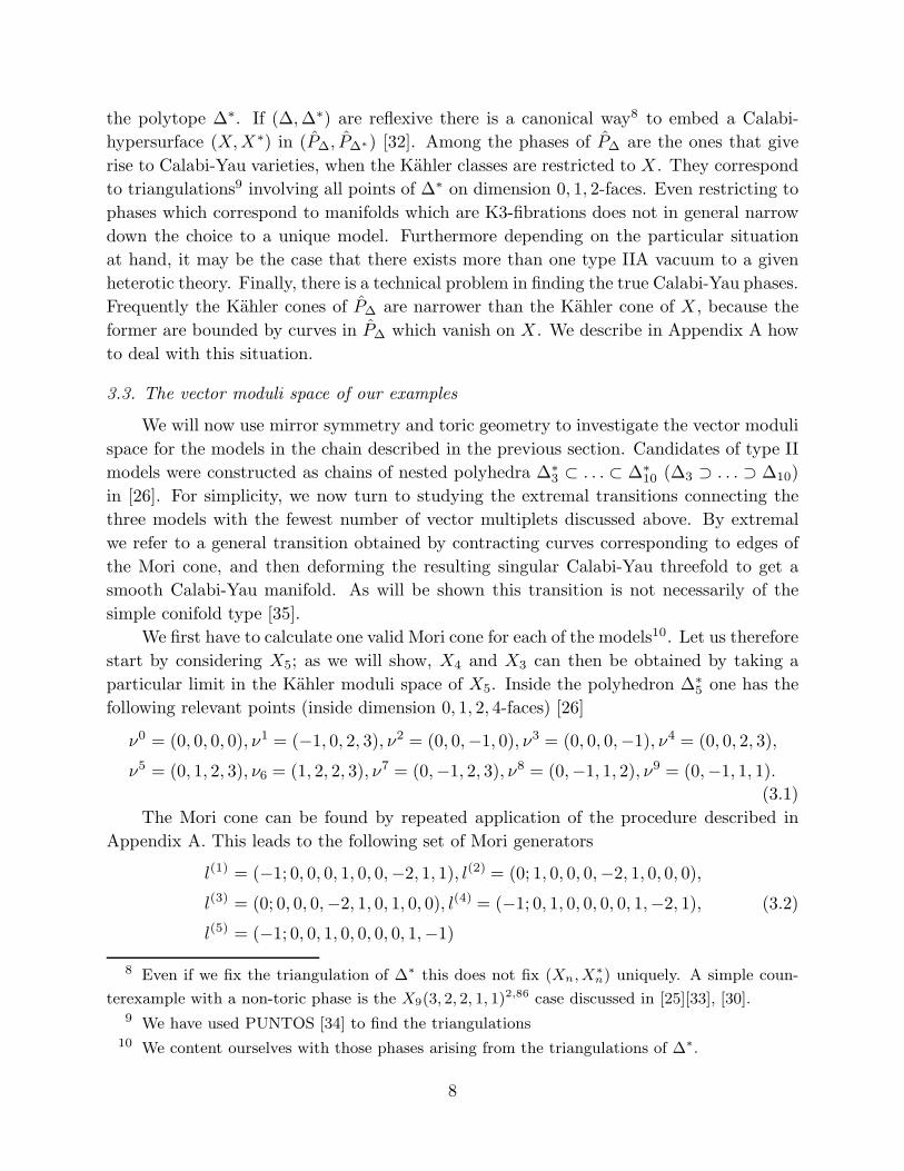
We first have to calculate one valid Mori cone for each of the models10. Let us therefore

start by considering X5; as we will show, X4 and X3 can then be obtained by taking a

particular limit in the Kahler moduli space of X5. Inside the polyhedron ∆∗5 one has the

following relevant points (inside dimension 0, 1, 2, 4-faces) [26]

ν0 = (0, 0, 0, 0), ν1 = (−1, 0, 2, 3), ν2 = (0, 0,−1, 0), ν3 = (0, 0, 0,−1), ν4 = (0, 0, 2, 3),

ν5 = (0, 1, 2, 3), ν6 = (1, 2, 2, 3), ν7 = (0,−1, 2, 3), ν8 = (0,−1, 1, 2), ν9 = (0,−1, 1, 1).

(3.1)

The Mori cone can be found by repeated application of the procedure described in

Appendix A. This leads to the following set of Mori generators

l(1) = (−1; 0, 0, 0, 1, 0, 0,−2, 1, 1), l(2) = (0; 1, 0, 0, 0,−2, 1, 0, 0, 0),

l(3) = (0; 0, 0, 0,−2, 1, 0, 1, 0, 0), l(4) = (−1; 0, 1, 0, 0, 0, 0, 1,−2, 1),

l(5) = (−1; 0, 0, 1, 0, 0, 0, 0, 1,−1)

(3.2)

8 Even if we fix the triangulation of ∆∗ this does not fix (Xn,X∗

n) uniquely. A simple coun-

terexample with a non-toric phase is the X9(3, 2, 2, 1, 1)2,86 case discussed in [25][33], [30].9 We have used PUNTOS [34] to find the triangulations

10 We content ourselves with those phases arising from the triangulations of ∆∗.

8

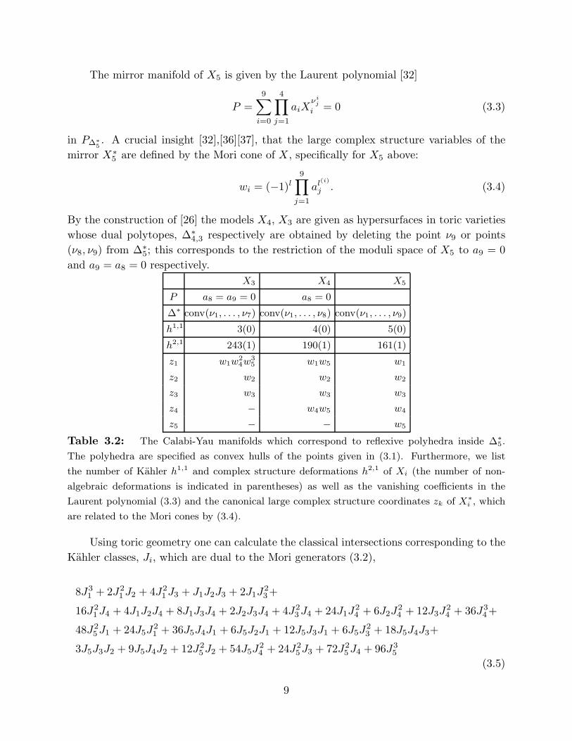
The mirror manifold of X5 is given by the Laurent polynomial [32]

P =9∑

i=0

4∏

j=1

aiXνi

j

i = 0 (3.3)

in P∆∗

5. A crucial insight [32],[36][37], that the large complex structure variables of the

mirror X∗5 are defined by the Mori cone of X , specifically for X5 above:

wi = (−1)l

9∏

j=1

al(i)

j . (3.4)

By the construction of [26] the models X4, X3 are given as hypersurfaces in toric varieties

whose dual polytopes, ∆∗4,3 respectively are obtained by deleting the point ν9 or points

(ν8, ν9) from ∆∗5; this corresponds to the restriction of the moduli space of X5 to a9 = 0

and a9 = a8 = 0 respectively.

X3 X4 X5

P a8 = a9 = 0 a8 = 0

∆∗ conv(ν1, . . . , ν7) conv(ν1, . . . , ν8) conv(ν1, . . . , ν9)

h1,1 3(0) 4(0) 5(0)

h2,1 243(1) 190(1) 161(1)

z1 w1w2

4w3

5 w1w5 w1

z2 w2 w2 w2

z3 w3 w3 w3

z4 − w4w5 w4

z5 − − w5

Table 3.2: The Calabi-Yau manifolds which correspond to reflexive polyhedra inside ∆∗

5.

The polyhedra are specified as convex hulls of the points given in (3.1). Furthermore, we list

the number of Kahler h1,1 and complex structure deformations h2,1 of Xi (the number of non-

algebraic deformations is indicated in parentheses) as well as the vanishing coefficients in the

Laurent polynomial (3.3) and the canonical large complex structure coordinates zk of X∗

i , which

are related to the Mori cones by (3.4).

Using toric geometry one can calculate the classical intersections corresponding to the

Kahler classes, Ji, which are dual to the Mori generators (3.2),

8J31 + 2J2

1 J2 + 4J21 J3 + J1J2J3 + 2J1J

23+

16J21J4 + 4J1J2J4 + 8J1J3J4 + 2J2J3J4 + 4J2

3 J4 + 24J1J24 + 6J2J

24 + 12J3J

24 + 36J3

4+

48J25J1 + 24J5J

21 + 36J5J4J1 + 6J5J2J1 + 12J5J3J1 + 6J5J

23 + 18J5J4J3+

3J5J3J2 + 9J5J4J2 + 12J25J2 + 54J5J

24 + 24J2

5J3 + 72J25J4 + 96J3

5

(3.5)

9

as well as the evaluation of the Chern class on the (1, 1) forms Ji,

c2(J1) = 92, c2(J2) = 24, c2(J3) = 48, c2(J4) = 132, c2(J5) = 168 (3.6)

Obviously the intersection numbers of X4 and X3 are simply given from these by

the restriction to the first four respectively three Kahler classes. For further studying the

transition we also need the Gromov-Witten invariant for the rational curves. These are

obtained from the solutions of the Picard-Fuchs equations using the mirror hypothesis and

listed in Appendix B.

3.4. Local geometry and summation of the instanton corrections

Let us begin with X3, and identify the associated toric variety P3.1112 A partial list

on the number of rational curves of low degree, including those of importance for studying

the transitions described in this paper, can be found in table A.1.

We will now show that this model is primitive, i.e. it does not admit a geometric

transition to a model with fewer Kahler parameters. Let us therefore discuss the edges of

the Mori cone one at a time, to determine whether their contraction admits a birational

smooth deformation. We start by studying the first edge of the Mori cone. This edge

describes curves contained in an elliptic fibration over a surface, so the contraction of

these curves is not a birational map (note that n1,0,0 = 480, the negative of the Euler

characteristic, as explained in [25]).

For our purposes, it is best to think of F2 as a complete toric variety with edges

(−1,−2), (1, 0), (0, 1), (0,−1). Its Mori cone is given by (−2, 0, 1, 0, 1), (0, 1,−2, 1, 0). As

such, it can be thought of as C4 − ({x1 = x6 = 0} ∪ {x5 = x7 = 0}) (in terms of the xi of

P3), modulo the (C∗)2 identification

(x1, x5, x6, x7) ∼ (tx1, st−2x5, tx6, sx7). (3.7)

The hyperplane class of F2 is the toric divisor x7 = 0, and will be denoted by H. We

can also think of F2 as the minimal desingularization of P(1, 1, 2), so it makes sense to

talk of the degree of a curve on F2. Note that a curve in the class dH has degree 2d.

In passing, we note that the exceptional divisor of this blowup, x5 = 0, is the section of

self-intersection −2.

11 This model has been studied earlier [38][12].12 In this section, we will frequently perform intersection calculations in the Calabi-Yau man-

ifolds Xk. These calculations are often inferred from the Mori cone; at times they may also be

performed by Schubert [39].

10

Returning to the first edge of the Mori cone, we note that the curve is contracted by

D1, D5, D6, D7.13 The relations D1 ·D6 = 0 and D5 ·D7 = 0, together with the C∗ actions

defining the toric variety, show that there is a map X3 → F2. The fibers are elliptic curves

with typical equation x23 +x3

2 +x2f16 +f24 = 0, where the fi have degree i in the variables

x1, x6, x7 of P(1, 1, 2), where x7 is the variable of degree 2.

The divisor D5 describes a ruled surface over an elliptic curve. This is the second

edge of the Mori cone. In this situation, the Gromov-Witten invariant is 2g − 2 = 0 [40].

There is no extremal transition in this case, although there is an SU(2) gauge symmetry

that is broken after a non-polynomial deformation [16]14.

Now we turn our attention to the divisor D4. The K3 fibration defined by (x1, x6)

restricts to D4 to describe D4 as a ruled surface over a genus 0 curve; the Gromov-Witten

invariant is n0,0,1 = 2g − 2 = −2, and there is no transition.

In summary, the Mori cone of X3 coincides with that of P3, and this model is primitive,

i.e. does not admit a geometric transition to a model with fewer Kahler parameters.15

This checks against the heterotic side, where the model with (nH , nV ) = (244, 4) is at the

bottom of the chain.

We next turn to the 4 parameter model X4. Some of the instanton numbers for this

model appear in table A.2. We will see that the fourth edge of the Mori cone is represented

by a conic bundle containing 28 line pairs, and that after contraction, there is a transition

to X3. From this transition, the Mori cone of X3 is the quotient of the Mori cone of X4

after modding out by the edge (0, 0, 0, 1). It remains to match up the edges from the

above geometry. The edges (0, 1, 0, 0) and (0, 1, 0) correspond to the ruled surface over

the elliptic curve, so are to be identified. The elliptic fibration identifies (1, 0, 0, 2) with

(1, 0, 0); or equivalently identifies (1, 0, 0, 0) with (1, 0, 0) due to the quotient. Finally, the

remaining edges (0, 0, 1, 0) and (0, 0, 1) are identified as ruled surfaces over rational curves.

From this, we infer the relation

na,b,c =∑

k

na,b,c,k (3.8)

which checks against the instanton numbers that we have provided, for example n1,0,0 =

−2 + 56 + 372 + 56 + −2 = 480.

13 Throughout our discussion, we will denote by Dk the restriction to Xi of the toric divisor

with equation xk = 0, when the model under discussion is clear from context.14 In [41][42] it was shown that turning on the non-polynomial deformation connects the moduli

space for X3 defined as an elliptic fibration over F2 (our case) with that of an elliptic fibration

over F0.15 Recent relevant geometric results about primitive Calabi-Yau threefolds have been given

in [43]

11

As we saw for X3, the model X4 also admits a map π : X4 → F2 defined by

(x1, x5, x6, x7x8). The fibers have type (1, 0, 0, 2) and are again elliptic. To calculate

this type, note that since x1 = x5 = 0 defines a point of F2, the same equation defines

an elliptic fiber of X4. We accordingly calculate the intersection numbers D1 ·D5 · Dk for

1 ≤ k ≤ 8, obtaining the Mori vector (−6; 0, 2, 3, 1, 0, 0, 0, 0), where the −6 arises because

the coordinates must sum to 0. In our basis for the Mori cone given in (A.5), this is just

(1, 0, 0, 2). Throughout this section, other classes have been computed in this manner;

the classes will be given without further comment. A curve C of type (0, 0, 0, 1) is also

contracted by π. Since C · D8 = −1, we see that C is necessarily contained in D8. Since

C · D7 = 1, there is a unique fiber of D7, a curve of type (1, 0, 0, 0) which meets C. This

curve is also contracted by π. The fiber of π containing both of these curves contains a

third component of type (0, 0, 0, 1); thus there are two curves of type (0, 0, 0, 1) in the same

fiber.

Because of C ⊂ D8, we restrict attention to D8, which admits a map to P1 by

restricting the K3 fibration defined by (x1, x6). After restricting to D8 (hence putting

x8 = 0), the equation of X4 becomes x22f8 + x2

3 + x27f16 + x2x3f4 + x2x7f12 + x3x7f8 = 0

where the fi have degree i in the variables x1, x6 of P1. We interpret the above as a family

of conics in the P2 with coordinates (x2, x3, x7), with (x1, x6) ∈ P1 as a parameter. The

discriminant of this family has degree 24. Thus the general fiber of D8 is a smooth conic

of type (0, 0, 0, 2), while there are 28 fibers where the conic splits into line pairs, each of

type (0, 0, 0, 1). As a check, note that n0,0,0,2 = −2 and n0,0,0,1 = 56.

The transition to X3 is found by writing down monomials in the variables of

P4 which have intersection number 0 with (0, 0, 0, 1). Choosing them in the order

(x1, x2x8, x3x8, x4, x5, x6, x7x8), we see that the assignment

(x1, . . . , x8) 7→ (x1, x2x8, x3x8, x4, x5, x6, x7x8)

defines a mapping from X4 to P3 which contracts the conic bundle, and takes X4 to a

singular form of X3. The transition is produced simply by deforming the equation of X3.

As a final comment on this model, we observe that the class of the elliptic fiber is

(1, 0, 0, 2). We have seen that the fiber of D7 is of type (1, 0, 0, 0), while the fiber of D8 is

of type (0, 0, 0, 2). The intersection of D7 and D8 meets either fiber in two points. Thus

D7 ∪ D8 is a fibration over P1 whose general fiber is a union of two P1s intersecting in

two points, while there are 28 special fibers which form triangles of curves. By itself, D8

is contracted to get X3, and this is the case N = 2, M = 28 of the geometry described in

Section 2.2. We accordingly expect to see 28 2 hyper multiplets becoming massless at the

transition, and that is in perfect agreement with Table 3.1.

Finally, we turn to the 5 parameter model X5. A partial list on low degree instanton

numbers, including those of importance for studying the transitions described in this paper

can be found in table A.3.

12

The key to understanding this transition is the contraction of the curves of type

(0, 0, 0, 0, 1). From table A.3 we have n0,0,0,0,1 = 30. This class has Mori vector

(−1, 0, 0, 1, 0, 0, 0, 0, 1,−1), so we see that this curve is contained in D9 = 0 and is con-

tracted by the divisors D1, D2, D4, D5, D6, D7. We also note from the first entry of the

Mori generators that the equation of X5 is in the class J1 + J4 + J5, where the Jk are the

dual generators of the Kahler cone. We accordingly write the equation of X5 in the form

x3f + x8g, (3.9)

where f is a polynomial with cohomology class J1 + J4 and g is a polynomial with co-

homology class 3J4. A curve is contracted by the divisors listed above if and only if

f = g = x9 = 0. We calculate D9 · (J1 + J4) · 3J4 = 30. Thus n0,0,0,0,1 = 30. The

transition to X4 is now visible—X4 is obtained from X5 by the map (x1 . . . , x9) 7→

(x1, x2, x3x9, x4, x5, x6, x7, x8x9).

The Mori cone of X4 is thus the quotient of the Mori cone of X5 by the vector

(0, 0, 0, 0, 1). We now match up the other edges. The edge (0, 1, 0, 0, 0) is the fiber of

a ruled surface over an elliptic curve, so corresponds to (0, 1, 0, 0). There is again an

elliptic fibration over P(1, 1, 2); we calculate that the fiber has class (1, 0, 0, 2, 3), which

is equivalent to (1, 0, 0, 2, 0) under the quotient. This must match with the elliptic class

(1, 0, 0, 2) of X4. This implies that (0, 0, 0, 1, 0) corresponds to (0, 0, 0, 1), and (1, 0, 0, 0, 0)

corresponds to (1, 0, 0, 0). The remaining edges (0, 0, 1, 0, 0) and (0, 0, 1, 0) are therefore

related; they are fibers of ruled surfaces over rational curves.

This gives the formula

na,b,c,d =∑

k

na,c,b,d,k (3.10)

which checks against the instanton numbers that we have provided, for example n1,0,0,0 =

−2 + 30 + 30 − 2 = 56.

As a final comment on this model, we observe that the class of the elliptic fiber is

(1, 0, 0, 2, 3). We have seen that the fiber of D7 is of type (1, 0, 0, 0, 0), while the fiber of D8

is of type (0, 0, 0, 1, 0). We can also calculate that the fiber of D9 has class (0, 0, 0, 1, 3). The

curves of type (0, 0, 0, 0, 1) are contained in degenerate fibers of D9; unlike the X4 situation,

the other component of this fiber is of a different type (0, 0, 0, 1, 2). The (0, 0, 0, 0, 1) curve

meets D8 but not D7, while the (0, 0, 0, 1, 2) curve meets D7 but not D8. Thus D7∪D8∪D9

is a degenerate elliptic fibration over P1 whose general fiber is a triangle. There are

30 special fibers where there is an extra component, and the fiber is a square of curves.

Together, D8 ∪D9 contract to give X3 (note that if we contract (0, 0, 0, 0, 1) together with

D8 to get X3, then we are contracting (0, 0, 0, 1, 0), hence the entire fibration D9 with class

(0, 0, 0, 1, 0) + 3(0, 0, 0, 0, 1)). This is the case N = 3, M = 30 of the geometry described

in Section 2.2. We accordingly expect to see 30 3 hyper multiplets becoming massless at

the transition, and that is in perfect agreement with Table 3.1.

13

We can also explicitly see for the X5 to X4 transition how the sets of three curves

change to sets of two curves as we go to X4. After contracting (0, 0, 0, 0, 1) to get to X4,

the two curves (0, 0, 0, 1, 0) and (0, 0, 0, 1, 2) pair up to become 30 pairs of (0, 0, 0, 1) curves.

In fact, it can be shown that the curve (0, 0, 0, 1, 2) is the “partner” of (0, 0, 0, 0, 1) under

the conic bundle. As the conic bundle gets smoothed out by the deformation process, there

are fewer lines pairs left.

We expect similar phenomena to arise for X6 and X7. For example, using the

P5(1, 1, 2, 6, 8, 10)[16, 12] model for X6, we have checked that the transition to the

P4(1, 1, 2, 6, 8)[18] model for X5 occurs by projection on the first 5 coordinates, and there

are M = 24 exceptional curves lying on a birationally ruled surface.

3.5. Physical interpretation of the examples

Let us now try to understand the above described transitions in a physical context.

We start with the X4 model. At the codimension one surface where the conic bundle is

contracted we have a singular P1 of type A1 with 28 double points of type A2. As we

will now argue, this corresponds to an infrared free theory SU(2) gauge theory with 28 2.

First, it has been shown in [19] [16] that a P1 bundle over a curve with singularity type

A1 gives an enhanced SU(2) gauge symmetry in the type IIA string theory. If the base

curve of the family is rational as in our case, it is also shown that there is no new matter

[16]. What we find here is that the contraction of the isolated curves, corresponding to

solitonic 2-branes wrapped around the curves becoming massless, gives rise to non-abelian

charged matter. The non-abelian charges arise from the fact that these isolated curves

originate from the same conic bundle as does the continuous family of rational curves

leading to the non-abelian gauge bosons. This is the non-abelian generalization of the

conifold singularity. As the SU(2) is Higgsed, the rank of the gauge group is reduced by

one, while the number of hyper multiplets increase by 53. This is seen very nicely from

the expression of the instanton numbers (3.8). Note how the fact that n0,0,0,2 = −2 fits

with losing two of the hyper multiplets as the W± of the SU(2) becoming massive. There

is of course as usual one hyper multiplet which is “eaten” as the U(1) gauge boson of the

Cartan subalgebra of SU(2) become massive. Note how this exactly matches the heterotic

description. At the transition from (191, 5) to (244, 4), the gauge group is SU(2)×U(1)4,

with 28 2 hyper multiplets under the SU(2). The transition occurs by Higgsing the SU(2).

In fact we can give a quite explicit map of the transition of the type II theory to that

on the heterotic side by analyzing the physical quantities such as the mirror maps, dis-

criminants and periods which determine the N = 2 effective action. The relation between

the Mori generators

l(3)1 = l

(4)1 + 2 l

(4)4 , l

(3)2 = l

(4)2 , l

(3)3 = l

(4)3 (3.11)

14

implies the following relations between the special and algebraic coordinates, in an obvious

notation:z(3)1 = z1 z2

4 , z(3)2 = z2, z

(3)3 = z3

t(3)1 = t1 + 2 t4, t

(3)2 = t2, t

(3)3 = t3 .

(3.12)

From the mirror maps we find

z4 ∼1

(1 − q4)2, z1 ∼ (1 − q4)

4

that is the transition takes indeed place at the boundary divisor z1 = 1/z4 = 0. In this

limit the data of X4 such as the periods and discriminants reduce to those of X3. It is

instructive to see the connection to the heterotic moduli. On the heterotic side, which

is realized in terms of a simple orbifold construction of K3 [14] one has in addition to

the dilaton S, the moduli of the torus T, U a Wilson line B. On these moduli acts the

perturbative T-duality group which in a similar model has been determined to be [44]:

T → T + 1, U → U + 1, B → B + 1, B → −B, T ↔ U ;

B → B − U, T → T + U − 2B, U → U,(3.13)

together with the generalization of the inversion element T → −1/T which is however

realized in a less obvious way on the physical expressions. We expect a similar modular

group realized in the present model, possibly up to some coefficients which depend on the

details of the compactification lattice. Indeed, matching (3.13) to the symmetries realized

on the physical couplings of the Calabi–Yau compactification, we find the identifications

t1 = T, t2 = S − T, t3 = U − T, t4 = B + U

where B has in fact period 2 U rather than U . As a check on our physical picture we note

that the Weyl symmetry element of the SU(2) subgroup of the E8 factor is not corrected

by non-perturbative string effects contrary to the mirror symmetry of the heterotic torus,

as expected.

The situation for X5 is similar but as the rank is larger there is now room for more

interesting phenomena. As for X4 we can obtain an SU(2) by shrinking down the divisor

D8. As this is not the conic bundle there are no degenerate fibers, i.e. we have a family

of curves parameterized by P1 which is reflected in n0,0,0,1,0 = −2. Hence, there is no

matter, and the unbroken SU(2) is present only in the perturbative theory. This agrees

with the general field theoretic picture, as discussed in section 2.1. When the rank of the

gauge group is 2, there is an SU(2) for φ1 = φ2 6= 0, where the φi are the scalar vevs of

the vector multiplets. If we in addition to contracting the instantons of degree (0, 0, 0, 1, 0)

also shrink those of type (0, 0, 0, 0, 1) we get a further enhancement, to SU(3) as well as 30

15

massless triplets. This can be seen as we are now forced to shrink down any combination

of instantons which have degree (0, 0, 0, k, l). Among the non-zero entries we find three

components which all have n(0,0,0,k,l) = 30. Thus, 3 times 30 massless particles, forming

30 3s under SU(3). As we Higgs the SU(3), the three components split into a set of two

which gives the 28 2s of the remaining SU(2) and 29 new singlet hyper multiplets. We have

then arrived at the SU(2) point of X4 discussed above. Once more this agrees perfectly

with the heterotic picture. At the transition from (162, 6) to (191, 5), the gauge group is

SU(3) × U(1)4, with 30 3 hyper multiplets under the SU(3). The transition occurs by

breaking the SU(3) to SU(2) just as described above.

Finally, it is possible to avoid the enhanced gauge symmetry, and restrict to a codi-

mension one surface where 30 isolated instantons of degree (0, 0, 0, 0, 1) shrink to zero.

This is the type IIA analog of the conifold transition in the type IIB string discussed by

Greene, Morrison and Strominger [45]. Here, there are 29 flat directions among the 30

hyper multiplets which become massless as the size of the instantons go to zero. Thus,

after Higgsing we are left with U(1)5 and 29 new singlets. This IIA transition description

was given in [16], and applies as well to a similar transition occuring in [25].

4. Discussion and Conclusions

In this paper we have given strong evidence for extremal transitions between type II

Calabi-Yau vacua, where the dual process in the heterotic string corresponds to Higgs-

ing16. In particular, we have found evidence for a very nice correspondence between the

appearance of enhanced SU(N) gauge symmetries and the corresponding matter struc-

ture on one hand, and the existence of a particular type of singularities in the Calabi-Yau

manifold. The geometrical structure in question is that of N − 2 rationally ruled surfaces

and a conic bundle with M degenerate fibers. As the fibers, which are P1s, shrink to zero,

particles appearing as BPS-saturated states of 2-branes wrapped around the P1s become

massless. The crucial point is the existence of the degenerate fibers as they are the source

of the massless matter transforming in the fundamental of the relevant gauge group. The

particular models considered in this paper are elliptically fibered Calabi-Yau manifolds.

However, it seems as if the existence of the conic bundles is independent of this fact. We

thus believe that this scenario is more general, and we are currently investigating such

models17.

16 In a recent paper, transitions between type II vacua related to the dual SO(32) heterotic

string have been discussed [46].17 It has become known to us that similar problems are to be discussed in a forthcoming paper

by Bershadsky et. al [47].

16

Finally, recall that the transitions are taking place in the perturbative region of the

heterotic string, i.e. in the limit of large base in the K3-fibration in the type II theory.

Thus, it still remains the possibility that there exist other K3-fibrations with the same

behaviour as the radius of the P1 becomes large [30].

Acknowledgments: We thank Philip Candelas, Anamaria Font, Wolfgang Lerche, Bong

Lian, Jan Louis, Fernando Quevedo, S-S. Roan, Rolf Schimmrigk, Andy Strominger, Bernd

Sturmfels, Stefan Theisen and S-T. Yau for useful discussions and in particular Dave

Morrison and Ronen Plesser for explanations on the relevant singularity structure. P.B.

would like to thank the Institute for Advanced Study where this work was iniated, and

the Institute for Theoretical Physics at the University of California at Santa Barbara and

the Department of Mathematics at Oklahoma State University for hospitality during parts

of this project. P.B. was supported by the DOE grant DE-FG02-90ER40542 and by the

National Science Foundation under grant No. PHY94-07194. S.K. was supported by NSF

grant DMS-9311386 and an NSA grant MDA904-96-1-0021.

Appendix A. The Kahler Cone: Toric Variety vs. Calabi-Yau Hypersurface

We will now explain the relation between phases, although different when thought of

as toric varieties, in fact are identical when restricted to the Calabi-Yau hypersurface. Let

us assume that we have two toric varietes, PI and PII , which are related to each other by

a flop, i.e. a surface/curve, C, is blown down on PI , and when passing through the wall

of the Kahler cone where PI and PII meet C reemerges in PII as a surface/curve, C. (In

terms of the complex structure moduli space of the mirror theory the flop is merely an

analytic continuation beyond the radius of convergence, corresponding to the walls of the

Kahler cone.) We are still, however, to restrict this process to that of the hypersurfaces XI

and XII . Indeed, if the restriction of C and C to XI and XII respectively is empty there

is nothing to be flopped and XI is isomorphic to XII . We then have to consider the new

Kahler cone as that of the union of the Kahler cones of the PI,II . This process is repeated

until we have a distinct set of inequivalent models. (In the example we will consider we

always find just one K3-fibration phase after applying the above scheme.)

Let us now apply the above idea to that of toric variety P4 From the dual polytope

∆∗4 one finds three Calabi-Yau phases which all are K3-fibrations. Their respective Mori

generators are given by

(0, 0,−1, 0, 1, 0, 0,−3, 3), (0, 1, 0, 0, 0,−2, 1, 0, 0),

(0, 0, 0, 0,−2, 1, 0, 1, 0), (−2, 0, 1, 1, 0, 0, 0, 1,−1)(A.1)

17

(0, 1, 0, 0, 0,−2, 1, 0, 0), (−2, 0, 0, 1, 1, 0, 0,−2, 2),

(0, 0, 1, 0,−1, 0, 0, 3,−3), (0, 0,−1, 0,−5, 3, 0, 0, 3)(A.2)

and(0, 0, 1, 0, 5,−3, 0, 0,−3), (0, 1, 0, 0, 0,−2, 1, 0, 0),

(0, 0, 0, 0,−2, 1, 0, 1, 0), (−2, 0, 0, 1, 1, 0, 0,−2, 2).(A.3)

The second toric variety is obtained from the third one by a birational transformation which

contracts the surface x2 = x4 = 0 on the second toric variety and resolves the resulting

singularity to the surface x5 = x8 = 0 on the third toric variety. But on the second model

for X4 we have D2 · D4 = 0, and on the second we have D5 · D8 = 0. This says that the

birational tranformation does not affect the hypersurface, which are therefore isomorphic.

So there is really just one Calabi-Yau phase coming from the two toric varieties described

by (A.2) and (A.3). Therefore the Kahler cone of the hypersurface is the union of the two

Kahler cones. Since the Mori cone is dual to the Kahler cone, we conclude that the actual

Mori cone is the intersection of the two Mori cones (A.2) and (A.3), which we calculate to

be(0, 1, 0, 0, 0,−2, 1, 0, 0), (−2, 0, 0, 1, 1, 0, 0,−2, 2),

(0, 0, 0, 0,−2, 1, 0, 1, 0), (0, 0, 1, 0,−1, 0, 0, 3,−3).(A.4)

However, this new toric variety is related to that of (A.1) by a flop as well; contracting

x4 = x8 = 0 in the above phase and then resolving the surface x2 = x7 = 0 in phase

I. However, just as in the previous case D4 · D8 = 0 when restricted to the Calabi-Yau

hypersurface in (A.4) and D2 · D7 = 0 on the hypersurface in phase I. Thus we are left

with just one Calabi-Yau phase given as a hypersurface in a toric variety where the Mori

cone is generated by

(−2, 0, 0, 1, 1, 0, 0,−2, 2), (0, 1, 0, 0, 0,−2, 1, 0, 0)

(0, 0, 0, 0,−2, 1, 0, 1, 0), (−2, 0, 1, 1, 0, 0, 0, 1,−1).(A.5)

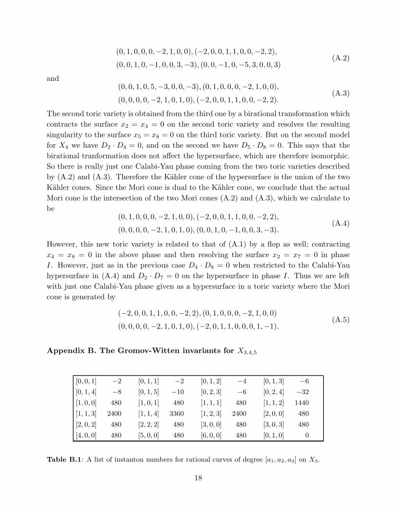
Appendix B. The Gromov-Witten invariants for X3,4,5

[0, 0, 1] −2 [0, 1, 1] −2 [0, 1, 2] −4 [0, 1, 3] −6

[0, 1, 4] −8 [0, 1, 5] −10 [0, 2, 3] −6 [0, 2, 4] −32

[1, 0, 0] 480 [1, 0, 1] 480 [1, 1, 1] 480 [1, 1, 2] 1440

[1, 1, 3] 2400 [1, 1, 4] 3360 [1, 2, 3] 2400 [2, 0, 0] 480

[2, 0, 2] 480 [2, 2, 2] 480 [3, 0, 0] 480 [3, 0, 3] 480

[4, 0, 0] 480 [5, 0, 0] 480 [6, 0, 0] 480 [0, 1, 0] 0

Table B.1: A list of instanton numbers for rational curves of degree [a1, a2, a3] on X3.

18

[0, 0, 0, 1] 56 [0, 0, 0, 2] −2 [0, 0, 0, 3] 0 [0, 0, 1, 0] −2

[0, 1, 0, 0] 0 [0, 1, 1, 0] −2 [0, 1, 2, 0] −4 [0, 1, 3, 0] −6

[0, 1, 4, 0] −8 [0, 1, 5, 0] −10 [0, 2, 3, 0] −6 [0, 2, 4, 0] −32

[0, 2, 5, 0] −110 [0, 2, 6, 0] −288 [0, 3, 4, 0] −8 [0, 3, 4, 0] −8

[0, 3, 5, 0] −110 [1, 0, 0, 0] −2 [1, 0, 0, 1] 56 [1, 0, 0, 2] 372

[1, 0, 0, 3] 56 [1, 0, 0, 4] −2 0

Table B.2: A list of instanton numbers for rational curves of degree [a1, a2, a3, a4] on X4.

[0, 0, 0, 0, 1] 30 [0, 0, 0, 0, 2] 0 [0, 0, 0, 1, 0] −2 [0, 0, 0, 1, 1] 30

[0, 0, 0, 1, 2] 30 [0, 0, 0, 1, 3] −2 [0, 0, 1, 0, 0] −2 [0, 1, 0, 0, 0] 0

[0, 1, 1, 0, 0] −2 [0, 1, 2, 0, 0] −4 [0, 1, 3, 0, 0] −6 [0, 1, 4, 0, 0] −8

[0, 2, 3, 0, 0] −6 [0, 2, 4, 0, 0] −32 [0, 2, 5, 0, 0] −110 [1, 0, 0, 0, 0] −2

[1, 0, 0, 1, 0] −2 [1, 0, 0, 1, 1] 30 [1, 0, 0, 1, 2] 30 [1, 0, 0, 1, 3] −2

[1, 0, 0, 2, 2] 30 [1, 0, 0, 2, 3] 312 [1, 0, 0, 2, 4] 30 [1, 0, 1, 0, 0] −2

[1, 0, 1, 1, 0] −2 [1, 0, 1, 1, 1] 30 [1, 0, 1, 1, 2] 30 [1, 0, 1, 1, 3] −2

Table B.3: A list of instanton numbers for rational curves of degree [a1, a2, a3, a4, a5] on X5.

19

References

[1] E. Witten, Nucl. Phys. B443 (1995) 85, hep-th/9503124.

[2] N. Seiberg, E. Witten, Nucl. Phys. B426 (1994) 19, hep-th/9407087.

[3] A. Klemm, W. Lerche, S. Theisen and S. Yankielowicz, Phys. Lett. 344 (1995) 169, P.

Argyres and A. Faraggi, Phys. Rev. Lett. 74 (1995) 3931; Ulf H. Danielsson, Bo Sund-

borg, Phys. Lett. 358B (1995) 273; A. Brandhuber, K. Landsteiner, Phys.Lett.B358

(1995) 73, R.G. Leigh, M.J. Strassler, Phys.Lett.B 356 (1995) 492; E. Martinec, N.

Warner, Nucl. Phys. B459 (1996) 97

[4] see e.g. C. Hull and P. Townsend, Nucl. Phys. B438 (1995) 109, hep-th 9410167

[5] S. Kachru and C. Vafa, Nucl. Phys. B450 (1995) 69, hep-th/9505105.

[6] S. Ferrara, J. Harvey, A. Strominger, and C. Vafa Second-Quantized Mirror Symmetry,

hep-th/9505162

[7] B. de Wit, P.G. Lauwers, R. Philippe, S.Q. Su, A. van Proeyen, Phys. Lett. 134B

(1984) 37; B. de Wit, A. van Proeyen, Nucl. Phys. B245 (1984) 89; J.P. Derendinger,

S. Ferrara, A. Masiero, A. van Proeyen, Phys. Lett. 140B (1984) 307; B. de Wit, P.G.

Lauwers, A. van Proeyen, Nucl. Phys. B255 (1985) 569; E. Cremmer, C. Kounnas,

A. van Proeyen, J.P. Derendinger, S. Ferrara, B. de Wit, L. Girardello, Nucl. Phys.

B250 (1985) 385

[8] J. Bagger, E. Witten, Nucl. Phys. B222 (1983) 1; J. Bagger, A. Galperin. E. Ivanov,

V. Ogievetsky, Nucl. Phys. B303 (1988) 522

[9] B. de Wit, V. Kaplunovsky, J. Louis and D. Lust, Nucl. Phys. B451 (1990) 53; I.

Antoniadis, S. Ferrara, E. Gava, K. S. Narain and T. R. Taylor, Nucl. Phys. B447

(1995) 35

[10] V. Kaplunovsky, J. Louis, and S. Theisen, Phys. Lett. 357 B (1995) 71; A. Klemm, W.

Lerche and P. Mayr, Phys. Lett. 357 B (1995) 313; C. Vafa and E. Witten, preprint

HUTP-95-A023; hep-th/9507050; I. Antoniadis, E. Gava, K. Narain and T. Taylor,

Nucl. Phys. B455 (1995) 109, B. Lian and S.T. Yau, Mirror Maps, Modular Relations

and Hypergeometric Series I,II, hep-th/9507151, hep-th 9507153;P. Aspinwall and J.

Louis, Phys. Lett. 369 B (1996) 233; I. Antoniadis, S. Ferrara and T. Taylor, Nucl.

Phys. B460 (1996) 489; G. Curio, Phys. Lett. 366 B (1996) 131, Phys. Lett. 366 B

(1996) 78; G. Lopes Cardoso, G. Curio, D. Lust and T. Mohaupt, Instanton Numbers

and Exchange Symmetries in N = 2 Dual String Pairs, hep-th/9603108

[11] S. Kachru, A. Klemm, W. Lerche, P. Mayr and C. Vafa, Nucl. Phys. B459 (1996) 537

[12] P. Aspinwall, Phys. Lett. 357 B (1995) 329, hep-th/9507012 ;

Enhanced Gauge Symmetries and Calabi-Yau Threefolds, hep-th/9511171.

[13] A. C. Avram, P. Candelas, D. Jancic, M. Mandelberg, On the connectedness of moduli

spaces of Calabi-Yau manifolds hep-th/9511230; T, Chiang, B. R. Greene, M. Gross,

20

Y. Kanter, Black hole condensation and the web of Calabi-Yau manifolds. hep-th

9511204

[14] G. Aldazabal , L.E. Ibanez , A. Font , F. Quevedo, Chains of N=2, D=4 heterotic/type

II duals, hep-th/9510093.

[15] P. Candelas and A. Font, Duality Between Webs of Heterotic and Type II Vacua,

hep-th/9603170.

[16] S. Katz , D. R. Morrison , M. R. Plesser, Enhanced Gauge Symmetry in Type II

String Theory, hep-th/9601108.

[17] A. Strominger, Massless Black Holes and Conifolds in String Theory , hep-th/9504090.

[18] M. Bershadsky , V. Sadov , C. Vafa, D-Strings on D-Manifolds, hep-th/9510225.

[19] A. Klemm and P. Mayr, Strong Coupling Singularities and Non-abelian Gauge Sym-

metries in N = 2 String Theory, hep-th/9601014.

[20] A. Klemm, W. Lerche, P. Mayr, C. Vafa and N. Warner, Selfdual Strings and N = 2

Supersymmetric Field Theory, hep-th/9604034

[21] D. R. Morrison and M. R. Plesser, private communication.

[22] R. Miranda, in The Birational Geometry of Degenerations, Progress in Math. vol. 29,

Birkhauser, 19983, 85.

[23] J. Harris, Algebraic Geomtry, Springer (1992) New York

[24] P. Aspinwall, B. Greene and D. Morrison, Nucl. Phys. B420 (1994) 184

[25] P. Berglund, S. Katz and A. Klemm, Nucl. Phys. B456 (1995) 153, hep-th/9506091.

[26] P. Candelas and A. Font, Duality Between Webs of Heterotic and Type II Vacua,

hep-th/9603170.

[27] D.R. Morrison, Through the looking glass, to appear.

[28] K. Oguiso, Internat. J. Math. 4 (1993) 439.

[29] B. Hunt and R. Schimmrigk, Heterotic Gauge Structure of Type II K3 Fibrations,

hep-th/9512138.

[30] P. Berglund, S. Katz, A. Klemm and P. Mayr, Type II Strings on Calabi-Yau Manifolds

and String Duality, in preparation.

[31] G. Aldazabal , A. Font , L.E. Ibanez , F. Quevedo, Heterotic/Heterotic Duality in

D=6,4, hep-th/9602097.

[32] V. Batyrev, Duke Math. Journal 69 (1993) 349, V. Batyrev, Journal Alg. Geom. 3

(1994) 493, V. Batyrev, Quantum Cohomology Rings of Toric Manifolds, preprint

1992

[33] S. Hosono, B.H.Lian, S.-T.Yau, GKZ Hypergeometric Systems and Applications to

Mirror Symmetry, alg-geom/9511001

[34] J. DeLoera, PUNTOS, ftp.geom.umn.edu/pub/software

[35] P. Aspinwall, An N=2 Dual Pair and a Phase Transition, hep-th/9510142.

[36] D. R. Morrison, hep-th 9311049; D. R. Morrison, P. Aspinwall, B.R. Greene, The

monomial divisor mirror map, hep-th/9407087

21

[37] S. Hosono, A. Klemm, S. Theisen and S.-T. Yau, Commun. Math. Phys. 167 (1995)

301, Nucl. Phys. B433 (1995) 501.

[38] A. Klemm, W. Lerche, P. Mayr, as cited in [10]

[39] S. Katz and S.A. Strømme. Schubert: a Maple package for intersection theory,

ftp.math.okstate.edu/pub/schubert

[40] P. Candelas, X. de la Ossa, A. Font, S. Katz and D. Morrison, Nucl. Phys. B416

(1994) 481, hep-th/9308083.

[41] D. R. Morrison and C. Vafa, Compactifications of F-Theory on Calabi–Yau Threefolds,

hep-th/96002114.

[42] P. S. Aspinwall and Mark Gross, Heterotic-Heterotic String Duality and Multiple K3

Fibrations, hep-th/9602118.

[43] M. Gross, Primitive Calabi-Yau Threefolds, alg-geom/9512002.

[44] P. Mayr and S. Stieberger, Phys. Lett. 355 B (1995) 107; G. Lopes Cardoso, D. Lust

and T. Mohaupt, Nucl. Phys. B432 (1994) 68

[45] B.R. Greene, D.R. Morrison, A. Strominger, Black Hole Condensation and the Unifi-

cation of String Vacua, hep-th/9504145.

[46] P. S. Aspinwall and M. Gross, The SO(32) Heterotic String on a K3 Surface, hep-

th/9605131.

[47] Bershadsky et. al, Geometric Singularities and Enhanced Gauge Symmetries, to ap-

pear.

22